2005-38Final Report

Analysis of Girder Differential Deflection and Web Gap Stress for Rapid Assessment of Distortional Fatigue in Multi-Girder Steel

Bridges

Technical Report Documentation Page1. Report No. 2. 3. Recipients Accession No.

MN/RC – 2005-38 4. Title and Subtitle 5. Report Date

October 2005 6.

Analysis of Girder Differential Deflection and Web Gap Stress for Rapid Assessment of Distortional Fatigue in Multi-Girder Steel Bridges 7. Author(s) 8. Performing Organization Report No.

Huijuan Li, Arturo E. Schultz 9. Performing Organization Name and Address 10. Project/Task/Work Unit No.

11. Contract (C) or Grant (G) No.

University of Minnesota, Institute of Technology Department of Civil Engineering 500 Pillsbury Drive South East Minneapolis, MN 55455 (C) 81655 wo) 120 12. Sponsoring Organization Name and Address 13. Type of Report and Period Covered

Final Report

14. Sponsoring Agency Code

Minnesota Department of Transportation Research Services Section 395 John Ireland Boulevard Mail Stop 330 St. Paul, Minnesota 55155

15. Supplementary Notes

http://www.lrrb.org/PDF/200538.pdf 16. Abstract (Limit: 200 words)

Distortion-induced fatigue cracking in unstiffened web gaps is common in steel bridges. Previous research by the Minnesota Department of Transportation (Mn/DOT) developed methods to predict the peak web gap stress and maximum differential deflection based upon field data and finite element analyses from two skew supported steel bridges with staggered bent-plate and cross-brace diaphragms, respectively. This project aimed to test the applicability of the proposed methods to a varied spectrum of bridges in the Mn/DOT inventory. An entire bridge model (macro-model) and a model encompassing a portion of the bridge surrounding the diaphragm (micro-model) were calibrated for two instrumented bridges. Dual-level analyses using the macro- and micro-models were performed to account for the uncertainties of boundary conditions. Parameter studies were conducted on the prototypical variations of the bridge models to define the sensitivity of diaphragm stress responses to typical diaphragm and bridge details. Based on these studies, the coefficient in the web gap stress formula was calibrated and a linear prediction of the coefficient was proposed for bridges with different span lengths. Additionally, the prediction of differential deflection was calibrated to include the influence of cross-brace diaphragms, truck loading configurations and additional sidewalk railings. A simple approximation was also proposed for the influence of web gap lateral deflection on web gap stress. 17. Document Analysis/Descriptors 18.Availability Statement

Bridge Girders Web Gap Stress Distortional Fatigue

Bent-Plate Diaphragm Cross-Brace Diaphragm Differential Deflection

No restrictions. Document available from: National Technical Information Services, Springfield, Virginia 22161

19. Security Class (this report) 20. Security Class (this page) 21. No. of Pages 22. Price

Unclassified Unclassified 113

Analysis of Girder Differential Deflection and Web Gap Stress for Rapid Assessment of Distortional

Fatigue in Multi-Girder Steel Bridges

Final Report

Prepared by: Huijuan Li

Arturo E. Schultz

Department of Civil Engineering University of Minnesota

October 2005

Published by:

Minnesota Department of Transportation Research Services Section

Mail Stop 330 395 John Ireland Boulevard

St. Paul, Minnesota 55155-1899

This report represents the results of research conducted by the authors and does not necessarily represent the view or policy of the Minnesota Department of Transportation and/or the Center for Transportation Studies. This report does not contain a standard or specified technique.

ACKNOWLEDGEMENTS

This research was made possible with the generous support from the Minnesota Department of

Transportation (Mn/DOT) and the Graduate School of the University of Minnesota. The author

would like to give many thanks to Paochen Mma, Erik Wolhowe, Barb Loida, Brian Homan and

Gary Peterson from the Mn/DOT Office of Bridges and Structures for their help on the progress

of this project.

Great appreciation is also expressed to the previous researchers on this series of research, Evan

Berglund, Benjamin Severtson and Frederick Beukema for their valuable assistance to this

project. Without their previous work and findings, this project could not have been completed

efficiently. In particular, special thanks must be given to the advisor, Arturo E. Schultz, whose

expertise and guidance were essential to the success of this research. Finally, the author would

like to thank her dear friends and family, their support and advice are highly appreciated.

Table of Contents

Chapter 1 - Introduction .............................................................................................................. 1

1.1 Background............................................................................................................................... 1

1.2 Objectives and Scope................................................................................................................ 3

1.3 Outline ...................................................................................................................................... 4

Chapter 2 - Literature Review..................................................................................................... 6

2.1 Overview................................................................................................................................... 6

2.2 Stress Mechanism ..................................................................................................................... 6

2.3 Retrofitting................................................................................................................................ 9

2.4 Background of Mn/DOT Project ............................................................................................ 11

Chapter 3 - Dual-level Analyses of I94/I694 Bridge ................................................................ 17

3.1 Overview................................................................................................................................. 17

3.2 Diaphragm Modeling in Macro-Model................................................................................... 18

3.3 Calibration of Finite Element Micro-Model........................................................................... 22

3.4 Calculation with Calibrated Models ....................................................................................... 23

Chapter 4 - Dual-level Analyses of Plymouth Ave. Bridge ..................................................... 27

4.1 Overview................................................................................................................................. 27

4.2 Stiffener Modeling in Finite Element Micro-Model............................................................... 27

4.3 Calibration of Restraint Condition in Finite Element Micro-Model ...................................... 29

4.4 Calculation with Calibrated Models ....................................................................................... 32

Chapter 5 - Parameter Study and Stress Formula Calibration of Prototypical Variations of

I94/I694 Bridge............................................................................................................................ 34

5.1 Overview................................................................................................................................. 34

5.2 Diaphragm Parameter Study for I94/I694 Bridge................................................................... 34

5.3 Calibration of Stress Prediction Equation for I94/I694 Bridge .............................................. 36

5.4 Comparison of Peak Web Gap Stress Prediction Methods..................................................... 39

5.5 Bridge Parameter Study of Prototypical Variations of I94/I694 Bridge ................................ 41

5.6 Comparison of 50-kip and HS-20 Truck Loadings ................................................................ 46

5.7 Stresses from the Bridge Parameter Study of I94/I694 Bridge .............................................. 50

Chapter 6 - Parameter Study and Stress Formula Calibration of Prototypical Variations of

Plymouth Ave. Bridge................................................................................................................. 54

6.1 Overview................................................................................................................................. 54

6.2 Modification Factor for Differential Deflections of Cross-Brace Diaphragms...................... 55

6.3 Comparison of Maximum Differential Deflections for Bridges with Additional Sidewalk

Railing and Type J-Rail ................................................................................................................ 59

6.4 Diaphragm Parameter Study for Plymouth Ave. Bridge ........................................................ 62

6.5 Calibration of Stress Prediction Equation for Plymouth Ave. Bridge.................................... 63

6.6 Bridge Parameter Study of Prototypical Variations of Plymouth Ave. Bridge ...................... 66

6.7 Stresses from the Bridge Parameter Study of Plymouth Ave. Bridge .................................... 72

Chapter 7 - Discussion of Lateral Deflection............................................................................ 75

7.1 Overview................................................................................................................................. 75

7.2 FE Diaphragm Study of I94/I694 Bridge ............................................................................... 75

7.3 Approximating Web Gap Lateral Deflection.......................................................................... 80

7.4 FE Diaphragm Study of Plymouth Ave. Bridge ..................................................................... 82

7.5 Discussion............................................................................................................................... 85

Chapter 8 - Summary and Conclusions .................................................................................... 90

References.................................................................................................................................... 94

Appendix A: Assessment of Peak Web Gap Stress in Plymouth Ave. Bridge

1. Evaluating Girder Differential Deflection ...................................................................... A-1

2. Peak Web Gap Stress Assessment .................................................................................. A-2

List of Tables Table 2.1 Polynomial Equation Constants by Berglund [2] ........................................................ 13 Table 2.2 Polynomial Equation Constants by Severtson [3] ...................................................... 16 Table 3.1 FE Model Results for I94/I694 Bridge under Truck Load Sweep 1........................... 24 Table 4.1 FE Model Results for Plymouth Ave. Bridge under Truck Left-Lane Loading......... 32 Table 5.1 Diaphragm Parameters and FE Model Results for I94/I694 Bridge........................... 35 Table 5.2 Parameter Study Results Normalized by S/∆ for I94/I694 Bridge........................... 37 Table 5.3 Comparison of Prediction Equation with and without δ for I94/I694 Bridge........... 38 Table 5.4 Comparison of Peak Web Gap Stress Prediction Methods for I94/I694 Bridge ........ 41 Table 5.5 Coefficient C for Models with Girder Spacing S = 10.5 ft ......................................... 43 Table 5.6 Coefficient C for Models with Skew Angle 60° at Different Girder Spacings .......... 44 Table 5.7 Prediction of Coefficient C for Bent-Plate Diaphragms............................................. 46 Table 5.8 Peak Web Gap Stress Values for Girder Spacing S = 10.5 ft ..................................... 50 Table 5.9 Comparison of Peak Web Gap Stress for Different Girder Spacings......................... 52 Table 6.1 Differential Deflection Data for Parameter Study Models with Bent-Plate and Cross-Brace Diaphragms......................................................................................................................... 56 Table 6.2 Constants in Polynomial Equation 2.7 for Girder Spacing Between 8 ft and 9.25 ft . 59 Table 6.3 Differential Deflection Data for Bent-Plate Diaphragms in Parameter Study Models with J-Rail and Sidewalk Railing ................................................................................................. 60 Table 6.4 Diaphragm Parameters Studied and FE Model Results for Plymouth Ave. Bridge ... 63 Table 6.5 Parameter Study Results Normalized by ∆/S for Plymouth Ave. Bridge................... 64 Table 6.6 Comparison of Prediction Equation with and without δ for the Cross-Brace Diaphragm in Plymouth Ave. Bridge ........................................................................................... 66 Table 6.7 Dual-Level Analyses Results for Plymouth Ave. Bridge using Various Models (L=140, S=9.25, and βs =40°)........................................................................................... 68

Table 6.8 Calculation Results for Diaphragms H and J of Plymouth Ave. Bridge .................... 72 Table 6.9 Peak Web Gap Stress Values for Cross-Brace Diaphragms ( sβ = 40°) ..................... 73 Table 7.1 FE Model Results of Web Gap Deformation for the I94/I694 Bridge ....................... 77 Table 7.2 Constants in Equation 7.2 for Variations of I94/I694 Bridge..................................... 81 Table 7.3 FE Model Results of Web Gap Deformation for the Plymouth Ave. Bridge............. 82 Table 7.4 Constants in Equation 7.2 for Variations of Plymouth Ave. Bridge ......................... 85 Table 7.5 Comparison of Stress Prediction without and with Proposed Lateral Deflection for I94/I694 Bridge............................................................................................................................. 87 Table 7.6 Comparison of Stress Prediction without and with Proposed Lateral Deflection for Plymouth Ave. Bridge .................................................................................................................. 88

List of Figures Figure 1.1 Girder Web Gap Distortion ........................................................................................... 2 Figure 1.2 Differential Deflection of Adjacent Girders.................................................................. 2 Figure 2.1 Diaphragm Rotation and Web Gap Deflection According to Fisher [10]..................... 8 Figure 2.2 Retrofit Examples of Stiffening Web Gaps [14] ......................................................... 10 (a) Stiffening Web Gap by Welding Connection Plate to Girder Flange ..................................... 10 (b) Stiffening Web Gap by Bolting Connection Plate to Girder Flange....................................... 10 Figure 2.3 Repair Solution of Drilling Holes at the Crack Tips [14] ........................................... 11 Figure 3.1 Portion of the Macro-Model Showing the Location of the FE Micro-Model ............. 17 Figure 3.2 Calibrated FE Micro-Model Configuration and Applied Loads ................................. 18 Figure 3.3 Configuration of Typical Diaphragm Elements in Macro-Model............................... 18 (a) Single-Line Frame Element (b) Shell Elements........................................... 18 Figure 3.4 Portion of Macro-Model Showing Typical Diaphragm Elements .............................. 19 (a) Single-Line Frame Diaphragm Elements ................................................................................ 19 (b) Shell Diaphragm Elements...................................................................................................... 19 Figure 3.5 Truck Load Configurations (Sweeps) ......................................................................... 20 Figure 3.6 Sand Truck Axle Load Configuration (50-kip) ........................................................... 20 Figure 3.7 Differential Deflection of the Diaphragm Represented in Micro-Model.................... 21 Figure 3.8 Portion of the I94/I694 Bridge Represented in FE Micro-Model ............................... 21 Figure 3.9 FE Micro-Model of the Diaphragm Represented by Jajich [1] ................................... 22 Figure 3.10 Deformed Shape of Web Gap and Stiffener from Dual-Level Analysis................... 24 Figure 4.1 Stiffener Plate Modeling in FE Micro-Model ............................................................. 28 (a) Single-Shell Element (b) Three-Shell Elements............................... 28 Figure 4.2 Web Stress in Vertical Direction around Web-Gap Region (ksi) ............................... 29 (a) Single-Shell Element Stiffener Model..................................................................................... 29 (b) Three-Shell Elements Stiffener Model.................................................................................... 29 Figure 4.3 Truck Lane Configurations.......................................................................................... 30

Figure 4.4 Portion of the Plymouth Ave. Bridge Represented in FE Micro-Model..................... 30 Figure 4.5 FE Micro-Model of the Diaphragm Represented by Severtson [3] ............................ 31 Figure 5.1 Labeling Scheme for Diaphragms in Bridge Macro-Models ...................................... 41 Figure 5.2 Lane 1 Loading Obtuse Corner Effect......................................................................... 42 Figure 5.3 Linear Approximation of C for Diaphragms at Girder Spacing 10.5 ft ...................... 44 Figure 5.4 Values of Coefficient C at Different Diaphragm Locations........................................ 45 Figure 5.5 Axle Load Configuration of AASHTO HS-20 Truck ................................................. 47 Figure 5.6 Ratio of C under 50-kip/HS-20 Truck Loadings........................................................ 47 Figure 5.7 Ratio of Maximum Differential Deflections under 50-kip and HS-20 Truck Loadings....................................................................................................................................................... 48 Figure 5.8 Peak Web Gap Stresses, wgσ , under 50-kip and HS-20 Truck Loadings ................... 49 Figure 5.9 Peak Web Gap Stresses wgσ under 50-kip Truck Lane 1 Loading for S = 10.5 ft ..... 51 Figure 6.1 Correction Factor Rx for Maximum Differential Deflection in Cross-Brace Diaphragms ................................................................................................................................... 57 Figure 6.2 Modification Factor Rx for the Prediction of Maximum Differential Deflection in Cross-Brace Diaphragms .............................................................................................................. 58 (a) Influence of Girder Spacing .................................................................................................... 58 (b) Unified Correction Factor ....................................................................................................... 58 Figure 6.3 Typical Bridge Cross Sections Showing Two General Classes of Bridge Railings.... 59 (a) J-rail......................................................................................................................................... 59 (b) Sidewalk & F-rail Barrier........................................................................................................ 59 Figure 6.4 Correction Factor (Rd) for Prediction of Maximum Differential Deflection in Bridges with Sidewalk Railing................................................................................................................... 61 Figure 6.5 Influence of Skew Angle on Coefficient C ................................................................. 69 Figure 6.6 Coefficient C in the Stress Equation for Cross-Brace Diaphragms ............................ 70 (a) Diaphragms Near the Pier ....................................................................................................... 70 (b) Diaphragms Away From the Pier............................................................................................ 70

Figure 6.7 Framing Plan of Plymouth Ave. Spans 4 and 5 Highlighting Diaphragms A, H, O and J ............................................................................................................ 71 Figure 7.1 Variation in Web Thickness (tw) for the I94/I694 Bridge ........................................... 77 Figure 7.2 Variation in Flange Thickness (tf) for the I94/I694 Bridge ......................................... 78 Figure 7.3 Variation in Web Gap Length (g) for I94/I694 Bridge ............................................... 79 Figure 7.4 Variation in Differential Deflection (∆) for I94/I694 Bridge...................................... 79 Figure 7.5 Variation in Deck Thickness (td) for I94/I694 Bridge................................................. 80 Figure 7.6 Variation in Web Thickness (tw) for the Plymouth Ave. Bridge................................. 83 Figure 7.7 Variation in Flange Thickness (tf) for the Plymouth Ave. Bridge............................... 83 Figure 7.8 Variation in Web Gap Length (g) for the Plymouth Ave. Bridge ............................... 84 Figure 7.9 Variation in Differential Deflection (∆) for Plymouth Ave. Bridge ........................... 84 Figure 7.10 Variation in Deck Thickness (td) for Plymouth Ave. Bridge .................................... 85

List of Equations Equation 2.1…………………… .................................................................................................... 8 Equation 2.2 .................................................................................................................................. 12 Equation 2.3…………………… .................................................................................................. 13 Equation 2.4…………………… .................................................................................................. 13 Equation 2.5…………………… .................................................................................................. 14 Equation 2.6…………………… .................................................................................................. 15 Equation 2.7…………………… .................................................................................................. 15 Equation 5.1…………………… .................................................................................................. 39 Equation 5.2…………………… .................................................................................................. 40 Equation 5.3(a) ……………………............................................................................................. 43 Equation 5.3(b) …………………… ............................................................................................ 43 Equation 5.4 .................................................................................................................................. 49 Equation 6.1…………………… .................................................................................................. 61 Equation 6.2…………………… .................................................................................................. 65 Equation 7.1…………………… .................................................................................................. 76 Equation 7.2………………………………………… .................................................................. 81 Equation 7.3…………………… …………………….................................................................. 86

Executive Summary Many multi-girder steel bridges built before the 1980s are experiencing distortion-induced

fatigue cracking at diaphragm-girder connections. The distortion-induced stresses in the

unstiffened web gap area that create the fatigue problems result from secondary forces developed

at the ends of the diaphragms as a result of relative deflections between the girders. Cracking

due to distortional fatigue seldom results in catastrophic failure of multi-girder steel highway

bridges, but its occurrence is frequent enough in the bridge inventory of the Minnesota

Department of Transportation (Mn/DOT) to warrant the development of an expedient and

accurate procedure for the assessment of this problem. Previous research of Mn/DOT has

developed two simple equations for the peak web gap stress based upon field monitoring and

finite element modeling of the instrumented portions of two skew-supported, multiple-girder

bridges. A method for the prediction of maximum differential deflection has been proposed

from the results of an extensive parameter study using finite element models of the entire bridges,

and a correction factor has also been suggested to account for the reduction effect of cross-brace

diaphragms on the prediction of maximum differential deflection compared with bent-plate

diaphragms.

This research project was designed to refine and reformulate, if necessary, the previously

developed equations for estimating stresses in steel girder webs due to out-of-plane distortion.

To resolve the uncertainties of boundary conditions introduced by disconnecting a portion of the

bridge from its connecting members, this project introduced dual-level analyses including both

macro-models (i.e., encompassing the entire bridge) and micro-models (i.e., encompassing a

portion of bridge surrounding the diaphragms in question) of the two field-monitored bridges.

The girder and deck rotations from macro-model analysis were identified as the rotational

restraint to be applied in the micro-models. Thus, the finite element macro- and micro-models of

the two field-monitored bridges were calibrated through dual-level analyses and the data on

diaphragm response to bridge loads were developed. Based upon the web gap behavior found

from dual-level analyses and the data recorded in the finite element analyses, the slope deflection

equation from linear beam theory was selected for future parameter studies on stress calculation.

With the calibrated models, dual-level analyses were performed on prototypical variations of the

instrumented bridges to define the sensitivity of diaphragm stress response to typical diaphragm

parameters (i.e., web thickness, web gap length, girder flange thickness, deck thickness, girder

differential deflection) and bridge parameters (i.e., span length, girder spacing, angle of skew). It

was found that the terms including web gap top and bottom rotations in the stress formula could

be approximated by linear functions of the ratio of differential deflection to girder spacing, thus a

coefficient (web gap rotation coefficient) was defined to represent the web gap rotation terms in

the stress formula, normalized by the ratio of differential deflection to girder spacing. A

comparison was made for different stress prediction methods proposed previously, and dual-level

analysis gave the best prediction of the finite element result. The research indicates that the

coefficient depends mainly on span length, with no obvious trend to varying skew angle and

girder spacing. In the parameter study of bridges with bent-plate diaphragms, a linear formula

that is a function of span length was proposed for diaphragms near to and away from the piers for

the prediction of the web gap rotation coefficient. In addition, the differential deflections under

different truck loadings were compared and a modification factor was proposed to account for

the influence of different truck loading configurations. In the parameter study of bridges with

cross-brace diaphragms, the correction factor for the prediction of differential deflections in

bridges with cross-brace diaphragms was recalibrated by considering different values for girder

spacing. The amounts and locations of maximum differential deflections for bridges with

sidewalk railing were also compared with those with J-rail to get further calibration. And the

linear formula of the web gap rotation coefficient was found to be appropriate for the prediction

of web gap stress of both bent-plate and cross-brace diaphragms.

Finally, since the lateral deflection of the web gap was neglected in the above stress prediction

equation, the values of lateral deflections recorded in diaphragm parameter study were analyzed

and a multivariate linear approximation was suggested to estimate the influence of lateral

deflection on web gap stress for each bridge respectively.

1

Chapter 1 - Introduction

1.1 Background

In many parts of the United States, steel multi-girder bridges with composite concrete decks are

the dominant form used for medium- and long-span bridges. The steel-reinforced concrete deck

is rigidly attached to the girders via shear studs embedded in the concrete. Transverse steel

members referred to as diaphragms between girders are intended to resist lateral loads and brace

the girders against lateral buckling during the construction process, as well as in the negative

moment region during the service life of bridges. The deck, diaphragms and transverse stiffener

plates also act to distribute loads laterally between bridge girders.

To avoid overlapping girder web-to-stiffener welds with welds at the girder flange and web

connection, transverse stiffeners are commonly terminated a few inches away from the girder

flange (Figure 1.1). A small portion of the girder web is left unstiffened because of this design

practice and it is known as a web gap (Figure 1.1). Prior to 1985, the connection of transverse

stiffeners to the girder tension flange was discouraged due to fatigue concerns. In general,

bridges experience differential deflections between adjacent girders especially for skew-

supported bridges, since the distance from an applied load to the nearest support varies from

girder to girder (Figure1.2).

Diaphragms connecting adjacent girders, owing to their high stiffness, undergo rigid body

rotations due to the imposed differential deflection between the connected girders. This rotation

forces the girder webs to experience an out-of-plane deformation, i.e., distortion (Figures

1.1&1.2). The unstiffened web gap region attracts the majority of this out-of-plane distortion

because of its relative flexibility and this occurs especially in negative moment regions where the

top flange is fully restrained by a stiff concrete deck. Large stresses can be generated at the toe

of the transfer stiffener in the web gap region from the out-of-plane distortion. Due to the cyclic

nature of stresses and the prevalence of this detail, distortion-induced fatigue cracking in

unstiffened web gaps is considered the largest source of fatigue cracking in steel bridges.

2

diaphragm stiffener(connection plate)

top flange

web

webgap

distortion

Figure 1.1 Girder Web Gap Distortion

Figure 1.2 Differential Deflection of Adjacent Girders

Much research has been conducted to address the sources, mechanisms and magnitudes of

distortional stresses and a variety of solutions have been proposed and implemented to alleviate

the problem. Though existing design codes offer solutions to mitigate distortional fatigue

damage, there is still little guidance on how to identify vulnerable structures and assess the

magnitude of distortional fatigue stress. Further research is required for this purpose.

S

∆

diaphragm

3

1.2 Objectives and Scope

Although many experimental studies have been previously conducted to investigate the fatigue

behavior and repair performance of the details subjected to out-of-plane distortion, there has

been little research expended towards a comprehensive understanding of bridge characteristics

responsible for this phenomenon and a simple method to predict the amount of web gap stress.

Previous research funded by the Minnesota Department of Transportation (Mn/DOT) developed

a simple equation for the prediction of peak web gap stress through field testing and subsequent

finite element modeling of a portion of the skew-supported bridge [1]. The subsequent project

funded by Mn/DOT led to the development of a formula for predicting diaphragm differential

deflection by an extensive parameter study on finite element models of bridges [2]. After that,

Mn/DOT funded another project to field-monitor two bridges with different geometries from

previous research. This research project created a simple stress prediction formula for the skew-

supported bridge with cross-braced diaphragms, and then proposed a correction factor for the

prediction of maximum differential deflection in cross-brace diaphragms from the formula for

bent-plate diaphragms obtained in previous research [3].

Given the state of knowledge described above, a project was funded by Mn/DOT to test the

applicability of previous research to a wide variety of steel bridges in the Mn/DOT inventory.

This thesis was written on the basis of the research conducted for the above purpose. The overall

goal of the project was to modify or reformulate, if necessary, the maximum web gap stress and

the differential deflection formulas to improve estimation accuracy over a wide variety of steel

bridges in the Mn/DOT inventory. To achieve this goal, the present project was initiated to

investigate and improve an analytical technique for simulating deck and girder rotational

restraint end conditions in the micro-model (i.e., encompassing a portion of bridge) with

calculated response from a macro-model (i.e., encompassing the entire bridge) of the bridge first.

This technique was used to study those factors that have an influence on the magnitude of

maximum web gap stresses in multi-girder steel bridges on skewed supports and with various

diaphragm details. Based on these studies, maximum web gap stress and differential deflection

formulas were calibrated.

4

Micro-models and macro-models of the two bridges, for which distortional fatigue field data are

available (i.e., I94/I694 Bridge in Brooklyn Center and Plymouth Ave. Bridge in Minneapolis),

were developed, along with analyses of prototypical variations of these bridges. The macro-

models are finite element models of the bridges in their entirety, and since the bridge was not

subdivided, no uncertainties were introduced regarding boundary conditions, as was the case for

micro-models (i.e., substructure) models at the locations where the model was disconnected from

the rest of the bridge. However, detailed assessment of highly localized stresses and strains, such

as web distortional stresses, is not feasible with macro-models because the finite element mesh is

necessarily coarser than that in a micro-model.

Analysis of truck loading in the macro-models was used to determine the appropriate rotational

restraint for the deck and girders to be used in the micro-models. Knowledge of girder and deck

rotations allowed the analysis using micro-models of the bridge (i.e., substructure surrounding

the diaphragms in question). The smaller size of the micro-model enabled a much finer mesh,

which afforded a degree of detail in the micro-models that enabled precise calculation of web

gap stresses. Dual-level analyses of the field-monitored bridges (i.e., with both macro- and

micro-models) were used to calibrate the models. Analysis of prototypical variations served to

expand the population of applicable bridges. The computed web gap stresses and differential

deflections were used to calibrate the stress and deflection formulas for the rapid assessment

methodology.

1.3 Outline

This report begins with a brief introduction of the subject of distortional web gap stress in multi-

girder steel bridges. The objectives and scope of this research project and a brief outline of the

contents of this document are also included.

Chapter 2 gives a literature review of the problems associated with the out-of-plane distortion of

the web gap region and the efforts that have been made to understand and address the problem.

The previous Mn/DOT research projects, which serve as the initiation for this research and

which provide much useful information, are also summarized.

5

Chapter 3 discusses the dual-level analyses (including macro- and micro-models) of the I94/I694

Bridge in Brooklyn Center. The finite element models are calibrated and data on diaphragm

response to bridge loads is developed. The web gap stress equation based upon linear beam

theory is recommended for future calculation.

Chapter 4 performs the dual-level analyses (including macro- and micro-model) of the Plymouth

Ave. Bridge in Minneapolis. The finite element models are calibrated for this bridge. Data on

diaphragm response to bridge loads is also covered.

Chapter 5 describes the parameter study of prototypical variations of the I94/I694 Bridge. The

sensitivity of bent-plate diaphragm stress response to typical diaphragm and bridge parameters is

defined and the calibration of web gap rotation coefficient in the web gap stress formula is

proposed.

Chapter 6 presents the parameter study of prototypical variations of the Plymouth Ave. Bridge.

The prediction equation of differential deflection is calibrated for cross-brace diaphragms and

sidewalk railings. The sensitivity of cross-brace diaphragm stress response to typical diaphragm

and bridge parameters is studied and the recommendations on the estimation of peak web gap

stress are made.

Chapter 7 examines the lateral deflection data collected during the finite element diaphragm

parameter study of both the I94/I694 and the Plymouth Ave. Bridges, and an approximation is

proposed for the prediction of web gap lateral deflection relative to web gap rotations. Thus, the

influence of lateral deflection for varying diaphragm parameters on web gap stress is identified

for both bridges.

Chapter 8 reviews the conclusions of this research, and recommendations are provided for the

application of the findings and future investigations.

6

Chapter 2 - Literature Review

2.1 Overview

Problems associated with damage from distortion-induced fatigue in steel bridges have been well

documented in the technical literature. Most previous research is based on field observation of

sources of distortional stresses, severity of fatigue damage and common features to damaged

bridges. A less common category of the literature documents experimental laboratory work

providing a detailed examination of the causes of distortional-induced cracking and assessment

of the effectiveness of retrofit designs. Research in field observations and laboratory

experiments has prompted design code changes and proposed design guidelines for future

structures. The understanding of the nature and severity of the distortional fatigue problem has

been enhanced from the research documented in the literature, and the field and experimental

observations have provided guidance on the maintenance and design of steel bridges. In

numerous reports, retrofitting attempts to alleviate distortional stresses are also a common

subject. Computer finite element modeling analysis has also been used in recent years to identify

the susceptible details and it provides useful information for future repair investigations and field

test instrumentation.

2.2 Stress Mechanism

In multi-girder steel bridges built before and during the 1980s, distortion-induced web gap

cracking is a common problem. Until 1985, connection was rarely provided between the

transverse stiffener and the girder tension flange. This resulted in an abrupt stiffness change in

the small web gap, and it exposed the region to high-cyclic out-of plane distortion and large

localized stresses. Since 1985, such connections have typically been welded or have been rigidly

bolted. When adjacent girders undergo different amounts of vertical deflection, the differential

deflection, ∆ , causes the stiff diaphragms between girders to undergo a rigid body rotation

(Figure 1.2). Rotation of the diaphragm imposes large deformations on the web gap (Figure 1.1).

Localized regions of high distortional stresses result when web gaps must accommodate the

majority of diaphragm movement. Due to the severity of the cyclic stresses and the prevalence

7

of this detail, distortion-induced fatigue cracking in unstiffened web gaps is considered the

largest source of fatigue cracking in steel bridges [4].

There are numerous case studies of field investigations documenting the web-gap distortional

fatigue cracking problem, and these instances validate the stress mechanism that the ongoing

Mn/DOT research program has investigated [1, 2, 3] and reinforce the importance of giving

further research attention to this problem [5,6,7,8]. Fatigue cracks due to distortional stresses are

typically parallel to the primary bridge bending stresses in the longitudinal direction, and they

are not detrimental if the cracks are discovered and retrofitted before turning perpendicular (i.e.,

vertical or inclined) to the primary stresses [5]. It is noted that a transverse stiffener welded to

the tension flange has the same fatigue resistance as the problematic web gap detail [9]. The

smooth weld profile of the web-flange connection region results in much higher fatigue

resistance than the weld termination at the transverse stiffener, though the measured range of

web gap stress is typically higher at the web-flange weld connection than at the termination of

the stiffener. Thus, in short web gaps, most cracking originates in the weld bead extending

beyond the end of the connection plate, while in gaps longer than 1.5 in. the cracks tend to form

at the connection plate weld toe [9].

The magnitude of distortional stresses has been shown to be difficult to predict from field

investigations and experimental studies [1, 3, 5, 6, 7, 8]. In previous research by Fisher, web

gaps are postulated to behave much like short, fixed-fixed beams undergoing lateral

deflection,δ , without end rotations [10]. One can arrive at an approximation for the relationship

between differential deflection, ∆ , and distortional stresses in the web gap using the slope

deflection equation. Assuming that the deep diaphragm is assumed to undergo a rigid body

rotation about its base, and the relatively thin web gap takes up all out-of-plane deflection, one

can arrive at the relationship between δ and ∆ shown in Figure 2.1. Neglecting the component

of stress due to rotation of one end of the web gap under this assumption, one arrives at Equation

2.1 for the maximum out-of-plane web gap stress, wgσ [10]. In Equation 2.1, E is Young’s

Modulus, tw is the thickness of the web, h is the depth of the diaphragm, S is the girder spacing, g

is the length of the web gap and ∆ is the differential deflection between adjacent girders, as

shown in Figure 2.1.

8

∆

==

Sh

gEt

gEt ww

wg 22

33 δσ Equation 2.1

Unfortunately, quantifying distortional stresses is not as easy as the preceding discussion might

imply. The amount of differential deflection between two adjacent girders, ∆, is not easily

predicted because the transverse interaction of concrete decks, reinforcement, girders, and

diaphragms is difficult to represent without detailed finite element analysis. Web gap stresses

are not necessarily well predicted by Equation 2.1 even if differential deflections are known

because the diaphragm, stiffeners and surrounding structural elements also absorb some of the

out-of-plane movement. Out-of-plane deflection of the lower flange can accommodate most of

the diaphragm rotation, leaving the web gap free to rotate. Moreover, real distortional stress

mechanisms are often highly sensitive to small changes in geometry, and some reports have

noted erratic cracking behavior for web gaps with lengths less than five times the web thickness

[11]. The fact remains that the exact magnitude of distortional stresses is still difficult to predict

without field investigation.

δ

g

Figure 2.1 Diaphragm Rotation and Web Gap Deflection According to Fisher [10]

S

h

Sh ∆≈ δ

∆

9

2.3 Retrofitting

A number of localized failures have developed in steel bridge components due to fatigue during

the past several decades. Out-of-plane distortions in a small web gap at the diaphragm

connection plates are the cause of the largest category of cracking in steel bridges [9]. Much

research has been performed to develop methods for correcting the distortional fatigue problems.

Retrofitting solutions for distortional fatigue problems are typically based on one of two different

strategies: (1) Increasing the stiffness of the system to resist the stresses placed upon it; (2)

Increasing the flexibility of the system so as to reduce the concentration of stresses.

To increase the stiffness, positive attachment of the transverse stiffener plate to the girder (bolted

and/or welded plates, angles or tees) is effective in mitigating distortional stresses [8, 9, 12, 13,

14, 15]. Though various retrofit connection details have been shown to reduce web gap stresses

and arrest crack growth, implementation of these options proves to be expensive and challenging.

Welding is the easiest type of retrofit connection to achieve, but the quality of field welds is hard

to assure because of the overhead welding positions, preheat requirements, dirt accumulation and

corrosion during service life.

Closure of the bridge is required if welds are to be placed for the retrofit operations to reduce

structure movement. Bolted solutions are also undesirable in the field because accessing the top

flange in the negative moment region requires the removal of the reinforced concrete deck.

Rigid splice components are recommended for less rigid bolted connections (0.75 inches thick

angles or larger). Positive attachments to the flanges reduce out-of-plane distortion to acceptable

levels provided the web gap length is larger than 2 inches or 4 times the web thickness,

whichever is larger. The American Association of State and Highway Transportation Officials

(AASHTO) design specifications specify the positive attachment of transverse stiffeners to the

girder flanges [16]. In addition, National Cooperative Highway Research Program (NCHRP)

Report 299 [17] provides further guidance for the fatigue evaluation of steel bridges. Figures

2.2(a) and 2.2(b) show examples for welding and bolted detail repairs, respectively [14].

10

(a) Stiffening Web Gap by Welding Connection Plate to Girder Flange

(b) Stiffening Web Gap by Bolting Connection Plate to Girder Flange

Figure 2.2 Retrofit Examples of Stiffening Web Gaps [14]

The methods to increase the system flexibility include: increasing the web gap length; loosening

or removal of bolts from the diaphragm connection; and removal of the diaphragm. To be fully

effective in stopping distortion and crack growth, increases in the web gap length by removing a

portion of the transverse stiffener must be at least 20 times the web thickness. This method has

been shown to significantly reduce the growth rate of fatigue cracks [9]. Loosening of bolts

lowers the stiffness of the diaphragm connection and has been shown to reduce the out-of-plane

distortion and its corresponding stresses [18]. It should be noted that loosened bolts can become

completely free due to traffic vibrations, which would create the hazard of falling nuts and bolts.

Complete removal of the diaphragm would eliminate the secondary stresses that cause fatigue

cracks in the girder web, but it can also increase the in-plane bending stresses in the main girders.

Field testing of both completely- and partially-removed diaphragms for two bridges indicated a

11

15% increase in girder stress after the repair [19, 20]. Thus, diaphragm removal should be used

with caution because it may increase girder stresses, and care should also be taken to make sure

that girder stability is considered following diaphragm removal.

The traditional repair method for a girder crack consists of drilling a hole at the crack tip (Figure

2.3). It has also been shown that hole-drilling is effective at stopping crack propagation,

provided the distortional stress less than 15 ksi and the in-plane bending stress does not exceed 6

ksi [9]. The primary concern in placing the drilled holes is that the crack tip be removed from

the web plate, thus, proper location of the crack tip is essential prior to drilling.

Figure 2.3 Repair Solution of Drilling Holes at the Crack Tips [14]

2.4 Background of Mn/DOT Project

Due to the importance of web gap distortion and the prevalence of the distortional fatigue

problem, the Minnesota Department of Transportation (Mn/DOT) funded research from 1998 to

instrument and monitor Bridge #27734 (I94/I694 Bridge) at the intersection of Interstate

Highways 94 (I-94) and 694 (I-694) in Brooklyn Center, Minnesota [1]. Long-term monitoring

of the bridge under ambient traffic loading was performed to determine the stresses to which the

bridge is subjected. The response of the bridge under known loading was investigated by testing

of the bridge with fully loaded Mn/DOT sand trucks driving at highway speeds. This monitoring

resulted in web gap stress measurements that were 2-2.5 times large than the flange stresses. A

detailed finite element (FE) analysis of the web gap region indicated that the maximum stresses

12

were much higher than those recorded in the field. These discrepancies were explained by the

large stress gradient in the web gap region and the location of the strain gages in the field. It was

also found from the FE analysis that the out-of-plane distortion of the web gap was primarily

created by a rotation of the diaphragm about the termination of the transverse stiffener.

With the mechanism known, the web gap was modeled as a small fixed-fixed beam pivoting

about the toe of the stiffener plate. Translating all of the differential deflection between girders

into the diaphragm rotation yields a rotation θ = ∆/S, where ∆ is the girder differential deflection,

and S is the girder spacing (S is also equal to diaphragm length). The slope deflection equation

was modified according to the above deformation and the approximate equation shown below for

the prediction of peak web gap stress was obtained.

∆

⋅=

SgtE w

wg 2σ Equation 2.2

The same notation as in Equation 2.1 was used. This equation gives much more realistic results

than Equation 2.1, and correlates well with the FE analysis.

Knowing that the web gap stresses depend only on the geometric parameters of the bridge and

the differential deflection of adjacent girders at the diaphragm location, further research focused

on the method of predicting the diaphragm differential deflection. A three-dimensional finite

element model encompassing the entire bridge (i.e., macro-model) was created and refined to

model the recorded behavior of I94/I694 Bridge. With this refined model and modeling

guidelines from a survey of the Mn/DOT bridge inventory, primary and secondary parameter

studies were performed to determine the influence of various parameters on the differential

deflection of adjacent bridge girders [2]. The primary parameters in this research included girder

spacing, angle of skew and main span length, and the secondary parameters were concrete deck

thickness, adjacent span length and diaphragm depth, as well as additional values for girder

spacing that were not considered in the primary study. Maximum differential deflections were

found for bridge models in which the previously mentioned parameters were varied. It was found

that the magnitude of differential deflection changes with main span length, angle of skew, girder

13

spacing and concrete deck thickness. It was also observed that the maximum value of ∆/S

mainly depends on skew angle and span length. The polynomial equation in Equation 2.3 was

shown to give reasonably accurate estimates for differential deflection.

L

ALALAS

322

1 +⋅+⋅=

∆ Equation 2.3

The constants A1, A2 and A3 for skew angles equal to 20°, 40° and 60° are listed in Table 2.1. For other angles of skew, linear interpolation can be used to estimate the constants.

Modification factors were developed for Equation 2.3 based upon the weight of the truck being

considered as well as the thickness of the concrete deck.

Table 2.1 Polynomial Equation Constants by Berglund [2]

Constants (L in meters)(deg.) A1 A2 A3

20 -0.00001327 0.001486 -0.00863940 -0.00001227 0.001522 -0.0103460 -0.00001714 0.002185 -0.02328

(deg.) A1 A2

A3 20 -3.370E-07 0.001486 -0.3399

40 -3.115E-07 0.001522 -0.406560 -4.352E-07 0.002185 -0.9156

Constants (L in inches)

Berglund [2] also determined that if the actual web thickness or web gap length is not known,

Equation 2.4 can be used as an approximation for the ratio of web thickness to web gap length.

Equation 2.4 came from the survey of the Mn/DOT bridge inventory and should be used only

when actual bridge geometry is absent. In this equation K = -0.002858 when L is in meters and

-0.00007260 when L is in inches.

4091.0+⋅= LKgtw

Equation 2.4

From the two Mn/DOT research projects referenced above, the combination of Equations 2.2 and

2.3 allows for the prediction of the web gap stress based solely upon the geometry of the bridge

in question.

14

The stress prediction formula given by Equation 2.2 and the differential deflection prediction

method encompassed in Equation 2.3 are both based upon field data taken from I94/I694 Bridge

which is a three-span bridge with staggered bent-plate diaphragms and a skew angle of 60°. To

determine the relevance of the equations to other steel, multi-girder bridges on skewed supports

in the Mn/DOT inventory, two additional bridges were selected and instrumented to monitor

their distortional fatigue response [3]. Bridge #27796, which carries Plymouth Avenue over

Interstate Highway 94 and its ramps in Minneapolis, Minnesota, was selected. This five-span

bridge has a 45.5° angle of skew and staggered cross-brace diaphragms. In addition, Bridge

#62028, which conveys 7th Street over railroad tracks in St. Paul, Minnesota, was selected for

observation. This non-skew bridge has five spans with back-to-back bent-plate diaphragms.

Given the low amounts of differential deflection and stress measured during truck testing, as well

as knowledge of the mode of deformation that leads to higher stresses in the Plymouth Ave.

Bridge, it was believed that the 7th St. Bridge, and other non-skew bridges with back-to-back

diaphragms would not suffer from distortional fatigue problems.

The field study produced web gap stress measurements for the 7th St. Bridge and Plymouth Ave.

Bridge that were not well predicted by the Equations 2.1 and 2.2. This occurred because the

mode of out-of-plane deformation of both bridges was different from that assumed by previous

prediction methods. The proposed Equation 2.3 also did not predict accurately the differential

deflection measured during field testing of the Plymouth Ave. Bridge well. The study found that

the web gap stress was primarily generated by rotation of the top of the web gap, tθ , and rotation

of the bottom of the web gap, bθ . With the assumptions of linear beam theory, and considering

the web gap as a fixed-fixed isotropic beam, the slope deflection Equation 2.5 can be used as an

idealized representation of this system.

)32(gg

tEtb

wwg

δθθσ ++⋅

= Equation 2.5

A simplified version, given by Equation 2.6, was derived for the prediction of web gap stresses

based upon the finding of a parameter study performed using the finite element model of a

portion surrounding an instrumented diaphragm of the Plymouth Ave. Bridge. Normalizing by

15

∆/S the values from the parameter study for tθ , bθ gave fairly consistent results for the

variations in the top and bottom web gap rotations with web gap length, girder spacing, web

thickness and differential deflection. Thus, constant ratios of 1.7 and 0.9, respectively, were

proposed for the normalized rotations )//( St ∆θ and )//( Sb ∆θ . Equation 2.6 was based on this

finding. However, Equation 2.6 neglects the influence of lateral deflection of the web gap,δ ,

which some researchers have accredited as the major cause of the out-of-plane distortion of the

web gap, and Equation 2.1 was derived on the basis of this mechanism [10]. The reasons for

neglecting the lateral deflection were: (1) the accuracy of Equation 2.5 relative to field

measurements was not significantly affected by neglecting the lateral deflection; (2) in this

research and the finite element modeling performed by the previous Mn/DOT project [1], the

lateral deflection of the web gap was found to be negligible.

∆

⋅=

SgtE w

wg 5.3σ Equation 2.6

An understanding of the role of cross-braces in differential deflection was highlighted in the

second part of the project [3]. Specifically, the use of cross-braces in place of bent-plate

diaphragms significantly reduces maximum differential deflection. A parameter study showed

that the amount of that reduction is dependent on span length, and was used to develop a simple

factor, dependent only on span length, for reducing the deflection prediction of Equation 2.3 for

bridges with cross-brace diaphragms. A correction factor xR , given in Equation 2.7, was

proposed, where xR was defined as the ratio of differential deflection in bridges with cross-brace

diaphragms, cb∆ , to the differential deflection in bridges with bent-plate diaphragms, bp∆ .

That is, bpxcb R ∆=∆ and bp∆ is obtained from Equation 2.3. The constants B1 and B2 are listed

in Table 2.2.

LBLBRx ⋅+⋅+= 22

11 Equation 2.7

16

Table 2.2 Polynomial Equation Constants by Severtson [3]

It was suggested that there may be some correlation between girder spacing and the extent of

reduction in differential deflection afforded by cross-braces, and that this may be confirmed by

additional study. The project [3] has refined the ability to successfully assess the risk of

distortional fatigue in bridges with cross-brace diaphragms. Further research, however, is still

required to (1) verify the conclusions from this project, (2) calibrate the extant finite element

models and (3) evaluate the stress and differential deflection prediction equations so that their

use can be extended to applicable bridges in Mn/DOT inventory.

B1 B2

ft -1.931E-05 5.432E-04-1.341E-07 4.527E-05

m -2.078E-04 1.782E-03

Dimensionof L

Constants

in

17

Chapter 3 - Dual-level Analyses of I94/I694 Bridge

3.1 Overview

This chapter discusses dual-level finite element analyses of the I94/I694 Bridge (Bridge #27734)

in Brooklyn Center. Both the macro-model (i.e., encompassing the entire bridge) and micro-

model (i.e., encompassing a portion of bridge) finite element representations of the I94/I694

Bridge were studied using the SAP2000 software package.

Figure 3.1 Portion of the Macro-Model Showing the Location of the FE Micro-Model

The truck loads reported in Jajich’s field tests [1] were simulated and applied to the bridge

macro-model to determine the deformations to be imposed on the bridge micro-model. The

resulting deck rotations and diaphragm deflections from the macro-model finite element analyses

were used as boundary conditions for the micro-model finite element analyses at the locations

where these members were disconnected from the rest of the bridge (Figure 3.1). The loads were

applied to the micro-model in the form of a vertical displacement (equal to diaphragm deflection)

to all restraint nodes on the right girder and deck edge, and the rotation values from the macro-

Portion of Bridge Represented in the Micro-Model

Diaphragm

Pin Support (Pier)

West Abutment

18

model analysis for all restraint nodes on both deck edges about the line parallel to the girders

were superimposed on the micro-model (Figure 3.2).

Figure 3.2 Calibrated FE Micro-Model Configuration and Applied Loads

3.2 Diaphragm Modeling in Macro-Model

In previous research, Berglund [2] implemented a finite element modeling technique for three-

dimensional representation of the I94/I694 Bridge. Berglund modeled the bent-plate diaphragms

as single-line frame elements (Fig. 3.3(a) and 3.4(a)) which were connected solely at points in

the middle of the webs of adjacent girders. To investigate the appropriateness of this diaphragm

representation, a three-shell element model was used in the present study (Fig. 3.3(b) and 3.4(b)).

(a) Single-Line Frame Element (b) Shell Elements

Figure 3.3 Configuration of Typical Diaphragm Elements in Macro-Model

Rotation (R1)

Rotation (R1) Vertical Displacement (Diaphragm Deflection)

Pin

19

(a) Single-Line Frame Diaphragm Elements

(b) Shell Diaphragm Elements

Figure 3.4 Portion of Macro-Model Showing Typical Diaphragm Elements

Five different load cases were used by Berglund in previous research [2] to verify the

performance of his finite element macro-model (Figure 3.5). These truck configurations utilized

two 222-kN (50-kip) sand trucks crossing the bridge. The axle load distribution of one 50-kip

sand-filled truck applied on the macro-model is shown in Figure 3.6. All five of these truck

20

sweeps were tested using the two macro-models developed in the current project with the two

different diaphragm modeling techniques (Figures 3.3 & 3.4).

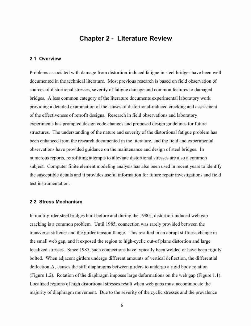
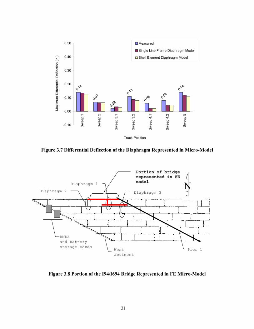
Figure 3.7 illustrates the deflection of the diaphragm represented using the two current micro-

models of the same bridge (Figure 3.8), for all truck sweeps. The resulting deflections of the

shell element diaphragm model are very close to the results in the single-line frame element

diaphragm model, and the latter are closer to measured values in most cases. Thus, the previous

diaphragm model (i.e., the single-line frame element) should not be changed to the more

complicated shell element model because the latter does not appear to provide improvements in

calculation accuracy.

1 3.2

4.12

3.1 4.2

5

Figure 3.5 Truck Load Configurations (Sweeps)

Figure 3.6 Sand Truck Axle Load Configuration (50-kip)

21

0.14

0.07

0.02

0.11

0.06 0.0

80.1

4

-0.10

0.00

0.10

0.20

0.30

0.40

0.50

Sw

eep

1

Sw

eep

2

Sw

eep

3.1

Sw

eep

3.2

Sw

eep

4.1

Sw

eep

4.2

Sw

eep

5

Truck Position

Max

imum

Diff

eren

tial D

efle

ctio

n (in

.)

Measured

Single Line Frame Diaphragm Model

Shell Element Diaphragm Model

Figure 3.7 Differential Deflection of the Diaphragm Represented in Micro-Model

Westiabutment

Pier 1

Diaphragm 2Diaphragm 1

Diaphragm 3

RMDAand batterystorage boxes

NPortion of bridgerepresented in FEmodel

Figure 3.8 Portion of the I94/I694 Bridge Represented in FE Micro-Model

22

3.3 Calibration of Finite Element Micro-Model

In previous research [1], Jajich created a simplified micro-model for the I94/I694 Bridge. The

model consisted of two adjacent girders, connected by a diaphragm. The simplified model did

not include girder top flanges and the portion of deck on top of the girders. Instead, Jajich

assumed that the top of the girder of the micro-model was restrained from movement in all

directions. Jajich was assuming that the concrete deck would serve as a restraint against any

girder top displacement arising from out-of-plane distortion, and loads were applied to the FE

model in the form of a vertical displacement (diaphragm deflection) to all restraint nodes on the

right girder (Figure 3.9). However, given that a major component of the web gap stress can be

generated by rotation of the girder top flange, neglecting this rotational stiffness might be

inappropriate in some cases.

Figure 3.9 FE Micro-Model of the Diaphragm Represented by Jajich [1]

The micro-model for the same portion of bridge was recreated in the current research. The

girder top flanges and the portion of the concrete deck connecting the two girder segments were

modeled as shell elements, and they were connected by rigid elements at closely-spaced intervals

to ensure that concrete deck and girders act integrally (i.e., in a composite manner). The deck

boundary was fixed from translation along the edges parallel to the girders (Figure 3.2). With

Fixed Top Flange

Pin Support

Pin Support

Vertical Diaplacement

23

both macro- and micro-models for this bridge available, the girder differential deflection and

deck edge node rotations can be found from the macro-model and then applied to the micro-

model to determine the web-gap movement and stress field.

3.4 Calculation with Calibrated Models

Figure 3.7 indicates that diaphragm deflection value was maximized under truck load

configuration 1 (Sweep 1), and the FE macro-model predicts a differential deflection that is

closest to the measured value for this truck sweep. Thus, truck Sweep 1 in Figure 3.5 with the

truck axle load distribution shown in Figure 3.6 was used for the macro-model analysis.

Deflection of Diaphragm 1 in Figure 3.8 under this load case is ∆ = 0.129 in., and the deck edge

node rotations about the line parallel to the girders (R1) in Figure 3.2 were found using the finite

element macro-model. Loads were applied to the FE micro-model in the form of a 0.129-inch

vertical displacement (the diaphragm deflection calculated from the macro-model under truck

load Sweep 1) to all restraint nodes on the girder and deck edge along the right boundary of the

bridge, as well as the previously computed rotations of the restraint nodes along both deck edges.

The deformations imposed on the boundaries of the micro-model were obtained from macro-

model analysis of the I94/I694 Bridge.

The calculated peak web gap stress in the finite element micro-model was found to be 15.94 ksi,

occurring at the centerline of the stiffener connection, and the stress field was observed to decay

rapidly in both the longitudinal and vertical directions away from this location. Since girder top

rotations were considered in the calibrated micro-model of the current project, the mode of web-

gap deformation was found to be different from that assumed by Jajich [1]. Jajich artificially

suppressed top rotation of the web gap in his model, and, thus, the rotation of the stiffener plate

and the stiffener end of the web gap were forced to be the primary source of web gap stress.

Dual-level analysis showed that the web gap experienced both top and bottom rotations, as well

as a small amount of out-of-plane lateral deflection (Figure 3.10), and this mode of

deformational response suggests that the stress formula proposed by Jajich needs reevaluation

and possible modification.

24

The following notation is used to describe the geometry, stresses and deformations of the web

gap region: web gap length (g); diaphragm deflection (equal to relative differential vertical

deflection between adjacent girders) (∆); lateral deflection of stiffener toe with respect to the top

flange (δ); girder spacing (S); web thickness (tw); rotation of the top of the web gap (θt); rotation

of the bottom of the web gap (θb); and the peak web gap stress (σwg). Table 3.1 shows the

calculated web gap stress, rotations and lateral deflection from the FE analysis under two 50-kip

sand trucks in load Sweep 1.

Figure 3.10 Deformed Shape of Web Gap and Stiffener from Dual-Level Analysis

Table 3.1 FE Model Results for I94/I694 Bridge under Truck Load Sweep 1

Load Case ∆ (in) wgσ (ksi) tθ bθ δ (in) Sweep 1 0.12874 15.94 0.00108 0.000746 -0.00021

The data in Table 3.1 are interpreted using the stress formula developed by Severtson [3] and

Jajich [1] in which the web gap is idealized as a simple beam that is subjected to one-way

bending as a result of out-of-plane distortion (Equation 2.5). In deriving this formula, linear

25

beam theory was used to establish a relationship between end-moments, rotations and lateral

deflection for the web gap region, and linear elasticity was used to define the web gap stress

from the end-moment and web gap geometry.

Substituting into Equation 2.5 the computed values for out-of-plane rotations (θt and θb) and

lateral deflection (δ) from the finite element analysis of the micro-model, and knowing that g =

2.5 in., tw = 0.5 in. and E = 29,000 ksi, gives σ = 13.45 ksi. This computed hot spot stress is

reasonably close to the previously computed finite element value (σ = 15.94 ksi). Thus,

Equation 2.5 can be used to predict web gap stresses satisfactorily, and parameter studies in

Chapter 5 on stress calculation utilize this formula.

A web gap stress of 4 ksi (28MPa) under the same truck load case was measured by Jajich [1] in

the field test. According to Jajich [1] and Severtson [3], it is impossible to place strain gages at

the exact location where maximum web gap stress occurs (i.e., the center of the stiffener), due to

1) interference with the diaphragm stiffener on the front side of the connection, and 2) inability

to locate the centerline of the web gap and diaphragm stiffener on the back side of the connection.

Moreover, web gap stress decays rapidly around the stiffener-web connection area. Thus, peak

web gap stress generated by finite element analysis of the web gap, or by any prediction equation,

is likely to be much higher than the stress obtained from the field measurement. The calculated

maximum value is known as the “hot spot” stress.

Jajich [1] stated “The strain gage reading reflects not simply the value of strain at the center of

the gage, but an integrated average value of the vertical variation in strain across the gage length.

In the horizontal direction, the strain is larger to the left of the gage and smaller to the right and it

is therefore reasonable to assume that the average strain across the width of the gage is close to

the value at the center. In the vertical direction, however, strain decreases both above and below

and gage center, and measured stresses could be significantly lower than the hot-spot stress.

Calculations indicate an additional 25% reduction in measured stress due to this effect.” Thus,

incorporating the likely reduction in measured stress due to the vertical averaging of the strain

distribution, the field recorded stress of 4 ksi was found to correspond to approximately 75% of

the stress had it been measured at the center of the strain gage. That is to say, had a gage been

26

used that was infinitely short in the vertical direction, it would have measured a stress of 5.4 ksi

at the strain gage center (i.e., 75% of 5.4 ksi = 4 ksi). The actual experimental strain gage center

was placed 0.625 in. away from the stiffener plate centerline, and in the FE dual-level analysis, a

stress of 5.9 ksi was found at that location, for which the error is within 10%. Thus, the

horizontal distribution effect leads to a stress at the instrumented location which is 37% of the

hot spot stress (i.e., 37% of 15.94 ksi = 5.9 ksi). Alternatively, the measured stress can be

corrected for the both the vertical distribution and horizontal location effects, giving a

“measured” hot spot stress magnitude of 14.41 ksi (calculated as 4 ksi / 0.37 / 0.75) which

compares well with the FE result of 15.94 ksi (9.6% error).

Thus, the calibrated FE model for the I94/I694 Bridge was validated for future calculation.

Moreover, the maximum (i.e., hot spot) stress of 15.94 ksi from the FE study is about 2.9 times

the measured stress of 5.4 ksi, once the vertical distribution effect was incorporated into the

measured value (but neglecting the horizontal location effect). The maximum FE stress (15.94

ksi) is also about 4 times the measured stress of 4 ksi, if both the vertical distribution and

horizontal location effects are neglected.

27

Chapter 4 - Dual-level Analyses of Plymouth Ave. Bridge

4.1 Overview

This chapter discusses dual-level finite element analyses of the Plymouth Ave. Bridge (Bridge

#27796) in Minneapolis. Both the macro-model (i.e., encompassing the entire bridge) and

micro-model (i.e., encompassing a portion of bridge) finite element representations of the

Plymouth Ave. Bridge were studied and calibrated using the SAP2000 software package. The

truck loads reported in Severtson’s field tests [3] were simulated and applied to the bridge

macro-model to determine the deformations to be imposed on the bridge micro-model. The

resulting deck rotations and diaphragm deflections found through the macro-model finite

element analyses were used as boundary conditions for the micro-model finite element analyses

at the locations where these members were disconnected from the rest of the bridge (Figures 3.1

& 3.2). Web-gap stress and out-of-plane distortions of the girder web (i.e., girder web rotations

and lateral deflections) were calculated using the micro-model.

4.2 Stiffener Modeling in Finite Element Micro-Model

In previous research by Severtson [3], a finite element modeling technique was used in which the

transverse stiffener plate was modeled using a single shell element, the latter being a planar

element with zero thickness. The thickness of the stiffener plate (0.6125 in.) was used only to

determine the properties of the shell element, and not the topology (i.e., connectivity) to the rest

of the structure. The shell element representing the stiffener plate was placed at the centerline of

the stiffener in the actual structure (Figure 4.1(a)). The stiffener plate has a finite thickness in

the actual bridge, and it is joined to the girder web by fillet welds along both edges.

To study whether the single-shell element configuration is appropriate for analysis, a model

using three shell elements was used to represent the stiffener plate for comparison. The two

additional elements were added near the edges of the stiffener plate (Figure 4.1(b)). The three

elements were connected by rigid elements to act integrally, and they were rigidly connected to

the girder web to simulate the welded connection used in the actual system. The thickness of the

28

shell element at the centerline was taken as 0.5875 in., and both edges of the stiffener plate were

simulated using very thin shell elements with a thickness of 0.0125 in. A spacing equal to 0.3 in.

was used for the three elements (Figure 4.1 (b)) to model the actual geometry of the stiffener.

Weld dimensions, however, were not included in the topology of this model.

0.6125"

Shell Element

Rigid Elements

0.5875"

0.3"0.3"

0.0125"

Shell Elements

0.0125"

Rigid Elements

Shell Element

(a) Single-Shell Element (b) Three-Shell Elements

Figure 4.1 Stiffener Plate Modeling in FE Micro-Model

The maximum differential deflection measured by Severtson [3] during truck testing of the

Plymouth Ave. Bridge was applied to the pin supports of the right girder in the two FE micro-

models, each of these having a different stiffener model. The web-gap stress fields for these two

models are shown in Figure 4.2, and a 0.1-in. mesh was used in this connection region.

From the comparison of Figure 4.2 (a) and (b), the stress concentration at the centerline of

stiffener plate is widened approximately 0.1 in. on both edges with the addition of shell elements,

while the maximum stress in this region did not change much. Thus, the single-shell element

model for stiffener plates is appropriate if the goal of the analysis is the magnitude of the hot-

spot stress. For the remainder of this project, the shingle-shell element model for diaphragm

plates will be used for the sake of convenience and computational expedience.

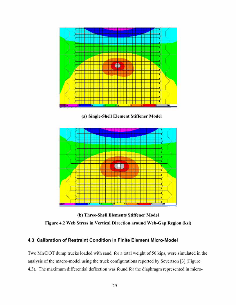
29

(a) Single-Shell Element Stiffener Model

(b) Three-Shell Elements Stiffener Model

Figure 4.2 Web Stress in Vertical Direction around Web-Gap Region (ksi)

4.3 Calibration of Restraint Condition in Finite Element Micro-Model

Two Mn/DOT dump trucks loaded with sand, for a total weight of 50 kips, were simulated in the

analysis of the macro-model using the truck configurations reported by Severtson [3] (Figure

4.3). The maximum differential deflection was found for the diaphragm represented in micro-

30

model and shown in Figure 4.4. The micro-model for the portion of Plymouth Ave. Bridge in

Figure 4.4 was calibrated such that the boundary conditions in the micro-model (i.e., the

displacements and rotations described earlier) were calculated from analysis of the macro-model.

Figure 4.3 Truck Lane Configurations

Figure 4.4 Portion of the Plymouth Ave. Bridge Represented in FE Micro-Model

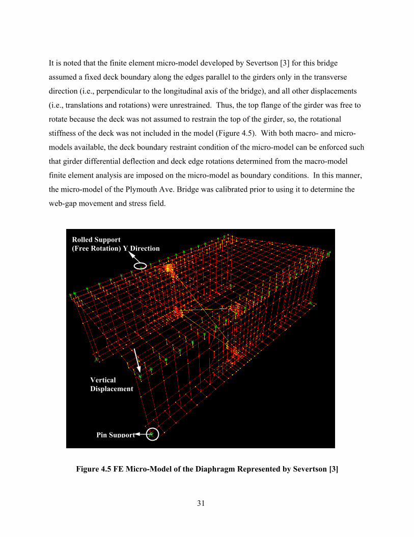
31

It is noted that the finite element micro-model developed by Severtson [3] for this bridge

assumed a fixed deck boundary along the edges parallel to the girders only in the transverse

direction (i.e., perpendicular to the longitudinal axis of the bridge), and all other displacements

(i.e., translations and rotations) were unrestrained. Thus, the top flange of the girder was free to

rotate because the deck was not assumed to restrain the top of the girder, so, the rotational

stiffness of the deck was not included in the model (Figure 4.5). With both macro- and micro-

models available, the deck boundary restraint condition of the micro-model can be enforced such

that girder differential deflection and deck edge rotations determined from the macro-model

finite element analysis are imposed on the micro-model as boundary conditions. In this manner,

the micro-model of the Plymouth Ave. Bridge was calibrated prior to using it to determine the

web-gap movement and stress field.

R

Figure 4.5 FE Micro-Model of the Diaphragm Represented by Severtson [3]

Rolled Support (Free Rotation) Y Direction

Pin Support

Vertical Displacement

32

4.4 Calculation with Calibrated Models

Macro-model analysis showed that the loaded diaphragm underwent maximum differential

deflection with the left-lane truck loading configuration (i.e., as reported by Severtson [3]). The

diaphragm deflection under this load case was ∆ = 0.0388 in., and the deck edge rotations about

the line parallel to the girders (R1) were found using the finite element macro-model. Loads

were applied to the FE micro-model in the form of a 0.0388-in. vertical displacement to all

restraint nodes on the right girder and deck edge, and the rotation values (from the macro-model

analysis) for all restraint nodes on both deck edges about the line parallel to the girders were

superimposed on the micro-model (Figure 3.2).

The calculated peak web-gap stress in the finite element model was found to be 8.23 ksi,

occurring at the centerline of the stiffener connection. Since girder top rotational stiffness was

considered in the present analysis of the calibrated micro-model, the calculated peak web-gap

stress is somewhat smaller than the value of 8.68 ksi, which was calculated using Severtson’s

micro-model (Figure 4.5). In Severtson’s micro-model, the lack of all rotational restraint along

the edges of the deck resulted in an overly flexible deck. Thus, the differential vertical deflection

of the girders at the diaphragm location produced more distortion of the web gap and larger out-

of-plane web stresses.

Table 4.1 shows the calculated web gap stress, rotation and lateral deflection from the FE models

under the 50-kip sand truck under left-lane loading. The following notation is used to describe

the geometry, stresses and deformations of the web gap region: web gap length (g); diaphragm

deflection (equal to differential vertical deflection of the adjacent girders (∆); lateral deflection

of stiffener toe with respect to the top flange (δ); girder spacing (S); web thickness (tw); rotation

of the top of the web gap (θt); rotation of the bottom of the web gap (θb); and the peak web gap

stress (σwg).

Table 4.1 FE Model Results for Plymouth Ave. Bridge under Truck Left-Lane Loading Load Case ∆ (in) wgσ (ksi) tθ bθ δ (in) Left-lane

33

The data in Table 4.1 is interpreted using the stress formula given by Equation 2.5. Substituting

into Equation 2.5 the web gap deformations computed from the micro-model analysis (θt, θb and

δ), and noting that g = 2.5 in., tw = 0.5625 in., and E = 29,000 ksi, gives σ wg = 6.25 ksi. This

computed hot spot stress is reasonably close to the previously computed finite element value (σwg

= 8.23 ksi). Thus, Equation 2.5 can be used to predict web gap stresses satisfactorily if the

vertical distribution and horizontal location effects (which are discussed below) are considered.

Thus, the parameter studies in Chapter 6 on stress calculation are based on this formula.

The field measurement of web gap stress (σ wg = 1.47 ksi) reported by Severtson [3] is much

lower than the FE dual-level analysis result because of the horizontal offset in strain gage

location relative to the centerline of the stiffener plate, as well as the rapid decay in stress with

vertical distance from the stiffener-web connection location. Due to a likely reduction of 25% in

measured stress due to the vertical averaging of web gap strain, as reported by Jajich [1] and

discussed in Chapter 3, the field recorded stress of 1.47 ksi was taken to be approximately 75%

of the measured stress at the center of the strain gage. Thus, the measured stress can be corrected

to a magnitude of 1.96 ksi at the strain gage center (1.96 ksi = 1.47 ksi / 0.75). Furthermore, the

strain gage was placed at a 0.75 in. horizontal offset from the stiffener plate centerline, and the

FE dual-level analysis generated a stress of 2.40 ksi at the strain gage location (i.e., at a 0.75 in.

offset), a value which is reasonably close to the measured value of 1.96 ksi (after vertical

distribution correction at the strain gage center).

Thus, the calibrated FE model for the Plymouth Ave. Bridge was validated for future calculation.

Additionally, the maximum stress of 8.23 ksi from FE study is about 4.2 times the measured

stress measured stress of 1.96 ksi, once the vertical distribution effect was incorporated into the

measured value (but neglecting the horizontal location effect). The maximum FE stress (8.23 ksi)

is also about 5.6 times the measured average stress of 1.47 ksi, if both the vertical distribution

and horizontal location effects are neglected.

34

Chapter 5 - Parameter Study and Stress Formula Calibration of Prototypical Variations of I94/I694 Bridge

5.1 Overview

This chapter comprises dual-level analyses and stress formula calibration for prototypical

variations of the I94/I694 Bridge in Brooklyn Center. The study discusses the sensitivity of

diaphragm stress response to prototypical variations of typical diaphragm and bridge parameters.

In the diaphragm parameter study, the web gap size, web thickness, girder flange thickness,

differential deflection and deck thickness of both the macro-model (i.e., encompassing the entire

bridge) and micro-model (i.e., encompassing a portion of bridge) finite element representations

for the I94/I694 Bridge were independently varied and the responses of the models were

monitored. By means of dual-level analyses, a refined calibration of the constant coefficient in

the stress formulas by Jajich [1] and Severtson [3] for bridges similar to the I94/I694 Bridge is

proposed. In the bridge parameter study, macro- and micro-models for bent-plate diaphragm

bridges consistent with Berglund’s guidelines for proportioning bridge models [2] were created

to study the influences of other parameters (i.e., angle of skew, main span length, girder spacing,

different truck configuration, diaphragm location) on web gap stress prediction. Coefficients in

the stress prediction formula were further calibrated and peak web gap stress estimates are

reported.

5.2 Diaphragm Parameter Study for I94/I694 Bridge

In previous research by Severtson [3], a parameter study was performed on the finite element

micro-model (i.e., encompassing a portion of bridge) of the Plymouth Ave. Bridge to study the

effects of web gap size, girder spacing, web thickness and the applied differential deflection (i.e.,

the diaphragm parameters), on peak web gap stress. A similar parameter study was performed

on the I94/I694 Bridge in this chapter with the calibrated macro- and micro-models described in

Chapter 3. The parameters varied here include web gap length, web thickness, deck thickness,

girder flange thickness, and diaphragm differential deflection. The values of the varied

35

parameters and the corresponding responses (i.e., peak web gap stress and web gap

deformations) are listed in Table 5.1, and the values contained in the original model (i.e., the

model that best represents the I94/I694 Bridge) are also noted as ‘Original’ in the first column.

The corresponding differential deflections calculated from the macro-model of I94/I694 Bridge

for varied web thickness, flange thickness and deck thickness are listed in the last column named

‘Note’ of Table 5.1.

Table 5.1 Diaphragm Parameters and FE Model Results for I94/I694 Bridge Parameter

Changed Value (in.) wgσ (ksi) tθ bθ δ (in.) Note

g 1.7 9.55 0.00108 0.000847 -0.0008 g 2 8.95 0.00108 0.000845 -0.00088 g 2.3 9.9 0.00108 0.000842 -0.00094

Original g 2.5 15.94 0.00108 0.000746 -0.00021 g 2.7 14.68 0.00108 0.000725 -0.00014 g 3 15.4 0.00108 0.000678 -0.00002 g 3.3 16.75 0.00108 0.000575 0.00011 tw 0.375 37.98 0.00115 0.000797 0.00261 ∆ =0.13699" tw 0.4375 24.26 0.00111 0.000766 0.00083 ∆ =0.13258"

Original tw 0.5 15.94 0.00108 0.000746 -0.00021 ∆ =0.12874" tw 0.5625 10.65 0.00104 0.000742 -0.00086 ∆ =0.12530" tw 0.625 7.22 0.001011 0.000742 -0.00126 ∆ =0.12218" tw 0.75 3.39 0.000968 0.000747 -0.00169 ∆ =0.11664"

Original ∆ 0.12874 15.94 0.00108 0.000746 -0.00021 Sweep 1 ∆ 0.11179 17.32 0.001085 0.000594 0.0002 Sweep5 ∆ 0.06517 7.33 0.000503 0.000397 -0.00019 Sweep2 ∆ 0.04658 5.36 0.000356 0.000287 -0.00013 Sweep 4.2 ∆ 0.03012 6.87 0.000393 0.000134 0.00026 Sweep 3.1 td 8 15.95 0.001075 0.000754 -0.00023 ∆ =0.12920"

Original td 9 15.94 0.00108 0.000746 -0.00021 ∆ =0.12874" td 10 13.56 0.000904 0.000606 -0.00013 ∆ =0.10529" tf 0.375 7.72 0.00164 0.00139 -0.00242 ∆ =0.19380" tf 0.5 9.51 0.00155 0.00127 -0.002 ∆ =0.18315" tf 0.625 11.16 0.00148 0.00118 -0.00166 ∆ =0.17419" tf 1.25 15.47 0.001095 0.000766 -0.00027 ∆ =0.13001" tf 1.5 19.04 0.001155 0.00076 0.0001 ∆ =0.13608" tf 2 20.22 0.000957 0.000575 0.00071 ∆ =0.11390" tf 2.375 23.84 0.00099 0.000565 0.000585 ∆ =0.11681"

Original tf 1.25/2.375 15.94 0.00108 0.000746 -0.00021 ∆ =0.12874"

36

The ranges of values for web thickness, deck thickness and girder flange thickness were selected

based upon the analysis of the Mn/DOT bridge inventory by Berglund [2]. Web gap lengths

were selected to represent the range of lengths found in Mn/DOT bridge inventory as well as

those reported by other researchers [3]. The differential deflection was varied by applying to the

macro-model of I94/I694 Bridge the five different loading sweeps described by Berglund [2].

The following notation is used to describe the geometry, stresses and deformations of the web

gap region: web gap length (g); diaphragm differential deflection (∆); lateral deflection of

stiffener toe with respect to the top flange (δ); web thickness (tw); girder flange thickness (tf);

deck thickness (td); rotation of the top of the web gap (θt); rotation of the bottom of the web gap

(θb); girder spacing (S); main span length (L); skew angle ( sβ ) and peak web gap stress (σwg).

The results of the parameter study (Table 5.1) deomstrate that all of the parameters studied have

an impact on the web gap stress. It is also noted that the values for both rotations (θt, θb) and the

lateral deflection of the web gap (δ) are affected by the variation of these parameters.

5.3 Calibration of Stress Prediction Equation for I94/I694 Bridge

From the dual-level analysis described in Chapter 3 of the I94/I694 Bridge, the mechanism of

distortional stress was found to be different from those assumed by Jajich [1] and Severtson [3].

The web gap experienced both top and bottom rotations and small amount of out-of-plane

deflection, and this fact suggests that the stress formulas proposed by Jajich and Severtson need

to be recalibrated. Equation 2.5 was investigated in Chapter 3, and it was found to be more

accurate than either of the web gap stress formulas proposed by Jajich or Severtson. Without

extensive field monitoring, the values for θb, θt, and δ for a bridge are difficult to determine, and

must be obtained in another manner. Severtson [3] found nearly constant values for )//( Sb ∆θ

and )//( St ∆θ from his parameter study results for the Plymouth Ave. Bridge. By neglecting δ,

he proposed the peak web gap stress prediction given by Equation 2.6 on the basis of Equation

2.5. To see whether Equation 2.6 can be used for the I94/I694 Bridge satisfactorily, or if it needs

to be calibrated, the values for θb, θt, and δ/g in Table 5.1 were normalized by S/∆ and listed in

37

Table 5.2. The values contained in the original model (i.e., the model that best represents the

I94/I694 Bridge) are also noted as ‘Original’ in the first column of Table 5.2.

Table 5.2 Parameter Study Results Normalized by S/∆ for I94/I694 Bridge

Parameter Changed Value (in.) )//( St ∆θ )//( Sb ∆θ

)//()/(S

g∆

δ

)//()2(

Stb

∆+ θθ

g 1.7 0.931 0.730 -0.406 2.39 g 2 0.931 0.728 -0.379 2.39 g 2.3 0.931 0.726 -0.352 2.38

Original g 2.5 0.931 0.643 -0.072 2.22 g 2.7 0.931 0.625 -0.045 2.18 g 3 0.931 0.585 -0.006 2.10 g 3.3 0.931 0.496 0.029 1.92 tw 0.375 0.932 0.646 0.846 2.22 tw 0.4375 0.929 0.641 0.278 2.21

Original tw 0.5 0.931 0.643 -0.072 2.22 tw 0.5625 0.921 0.657 -0.305 2.24 tw 0.625 0.918 0.674 -0.458 2.27 tw 0.75 0.921 0.710 -0.643 2.34

Original ∆ 0.12874 0.931 0.643 -0.072 2.22 ∆ 0.11179 1.077 0.589 0.079 2.26 ∆ 0.06517 0.857 0.677 -0.129 2.21 ∆ 0.04658 0.849 0.683 -0.124 2.22 ∆ 0.03012 1.450 0.493 0.383 2.44 td 8 0.924 0.648 -0.079 2.22

Original td 9 0.931 0.643 -0.072 2.22 td 10 0.953 0.639 -0.055 2.23 tf 0.375 0.939 0.796 -0.055 2.53 tf 0.5 0.939 0.770 -0.485 2.48 tf 0.625 0.943 0.752 -0.423 2.45 tf 1.25 0.935 0.654 -0.092 2.24 tf 1.5 0.942 0.620 0.033 2.18 tf 2 0.933 0.560 0.277 2.05 tf 2.375 0.941 0.537 0.222 2.02

Original tf 1.25/2.375 0.931 0.643 -0.072 2.22

The values for )//()2( Stb ∆+θθ listed in Table 5.2 are seen to be fairly consistent with respect

to all parameters that were varied, and much more so than for )//( Sb ∆θ and )//( St ∆θ . There is

no immediately obvious trend for )//()/( Sg ∆δ . By averaging the coefficients in the last column

of Table 5.2, an approximately constant value of 2.25 is determined for )//()2( Stb ∆+θθ . With

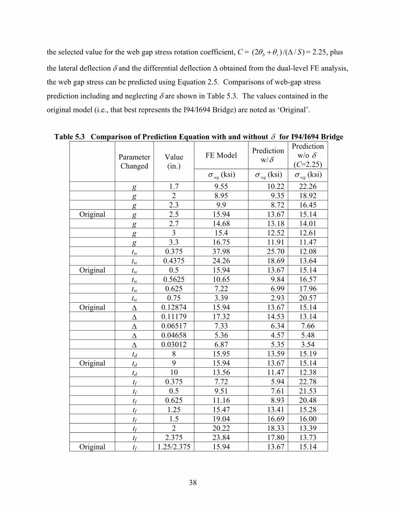
38

the selected value for the web gap stress rotation coefficient, C = )//()2( Stb ∆+θθ = 2.25, plus

the lateral deflection δ and the differential deflection ∆ obtained from the dual-level FE analysis,

the web gap stress can be predicted using Equation 2.5. Comparisons of web-gap stress

prediction including and neglecting δ are shown in Table 5.3. The values contained in the

original model (i.e., that best represents the I94/I694 Bridge) are noted as ‘Original’.

Table 5.3 Comparison of Prediction Equation with and without δ for I94/I694 Bridge

FE Model Prediction w/δ

Prediction w/o δ

(C=2.25) Parameter Changed

Value (in.)

wgσ (ksi) wgσ (ksi) wgσ (ksi) g 1.7 9.55 10.22 22.26 g 2 8.95 9.35 18.92 g 2.3 9.9 8.72 16.45

Original g 2.5 15.94 13.67 15.14 g 2.7 14.68 13.18 14.01 g 3 15.4 12.52 12.61 g 3.3 16.75 11.91 11.47 tw 0.375 37.98 25.70 12.08 tw 0.4375 24.26 18.69 13.64

Original tw 0.5 15.94 13.67 15.14 tw 0.5625 10.65 9.84 16.57 tw 0.625 7.22 6.99 17.96 tw 0.75 3.39 2.93 20.57

Original ∆ 0.12874 15.94 13.67 15.14 ∆ 0.11179 17.32 14.53 13.14 ∆ 0.06517 7.33 6.34 7.66 ∆ 0.04658 5.36 4.57 5.48 ∆ 0.03012 6.87 5.35 3.54 td 8 15.95 13.59 15.19

Original td 9 15.94 13.67 15.14 td 10 13.56 11.47 12.38 tf 0.375 7.72 5.94 22.78 tf 0.5 9.51 7.61 21.53 tf 0.625 11.16 8.93 20.48 tf 1.25 15.47 13.41 15.28 tf 1.5 19.04 16.69 16.00 tf 2 20.22 18.33 13.39 tf 2.375 23.84 17.80 13.73

Original tf 1.25/2.375 15.94 13.67 15.14

39

The results show that neglecting δ for varying values of ∆ and td does not significantly reduce

the accuracy of the stress prediction equation, except for extreme cases of short web gap lengths,

or very thin or very thick webs. For the cases in which tw, g and tf were varied, neglecting δ

caused the web gap stress prediction to have an inverse relationship with the model stresses.

However, in the field measurements of the I94/I694 Bridge reported by Jajich [1], no significant

lateral deflection δ of the web gap region was observed. Therefore, lacking a simple means to

predict δ with reasonable accuracy, as well as having reservations regarding its presence in the

response of actual bridges to vehicular loading, it is recommended that δ be neglected in the

stress prediction equation until a more comprehensive investigation of this parameter can be

made. Such investigation should include field data from a larger group of steel bridges on skew

supports, as well as finite element analysis of such bridges.

Using the selected value for C (i.e., C = )//()2( Stb ∆+θθ = 2.25), and neglecting the effect of δ

in Equation 2.5, leads to the proposed peak web gap stress prediction as given in Equation 5.1.

∆

=

SgtE w

wg 25.2σ Equation 5.1

Equation 5.1 can be used for bent-plate diaphragms similar to the diaphragms studied, and in

bridges with span length, skew angle and girder spacing similar to the I94/I694 Bridge. The

influence of the principal bridge parameters (i.e., span length, skew angle, and girder spacing) on

the prediction of web-gap stresses are discussed later in this chapter.

5.4 Comparison of Peak Web Gap Stress Prediction Methods

By now three different peak web gap stress prediction formulas have been developed, including

those proposed by Jajich [1] and Severtson [3], as well as Equation 5.1 proposed in the present

study on the basis of dual-level FE analyses. All of these formulas were based on linear beam

theory (i.e., Equation 2.5), and have a similar form:

40

∆

⋅=

SgtEC w

wgσ Equation 5.2

where C is a constant. Jajich [1] selected C=2 because rotation of the girder top flange (θt) in his

finite element model was fixed. Thus, only rotation of the bottom of the web gap (θb) was

considered, with the assumption that Sb /∆=θ in Equation 2.5, and lateral deflection of the web

gap δ was neglected. In this study, dual-level analyses were performed on the calibrated bridge

models, in which the portion of deck connecting the girders were modeled in the micro-model

and instead of fixing the girder top flange, rotations of the deck portion calculated from the

macro-model were applied to the micro-model as boundary condition. Both θt and θb were

included in the present study, and )2( tb θθ + = 2.25 )/( S∆ , thus the proposed value C=2.25 is

larger that proposed by Jajich’s (C=2).

Severtson [3] selected C=3.5 on the basis of his finite element analyses, and there are two

reasons for the marked difference between his proposed value for C compared with that proposed

in the present study (C=2.25) which was proposed for I94/I694 Bridge by means of dual level

analyses: First, Severtson’s parameter study was based on the micro-model of a cross-brace

diaphragm in the Plymouth Ave. Bridge, while the models studied in this document were based

on a bent-plate diaphragm in I94/I694 Bridge: The two bridges have different diaphragm

configurations and different geometric parameters. Second, Severtson did not consider the

rotational stiffness that could be contributed to the system by the portion of deck that was not

represented in his micro-model. Thus, the top flange of the girder in Severtson’s micro-model

was assumed to be free to rotate. This assumption leads to overestimated top rotations of the

web gap, θt, and web gap stresses, wgσ , compared with the results from dual-level FE analyses.

Knowing that g = 2.5 in., tw = 0.5 in., S = 111 in., E = 29,000 ksi and ∆ = 0.12874 in. under truck

sweep 1, the comparison of peak web gap stress predicted with different formulas is shown in

Table 5.4. From Table 5.4, the proposed Equation 5.1 is seen to offer the best prediction of the

peak web gap stress given by the dual-level FE analysis.

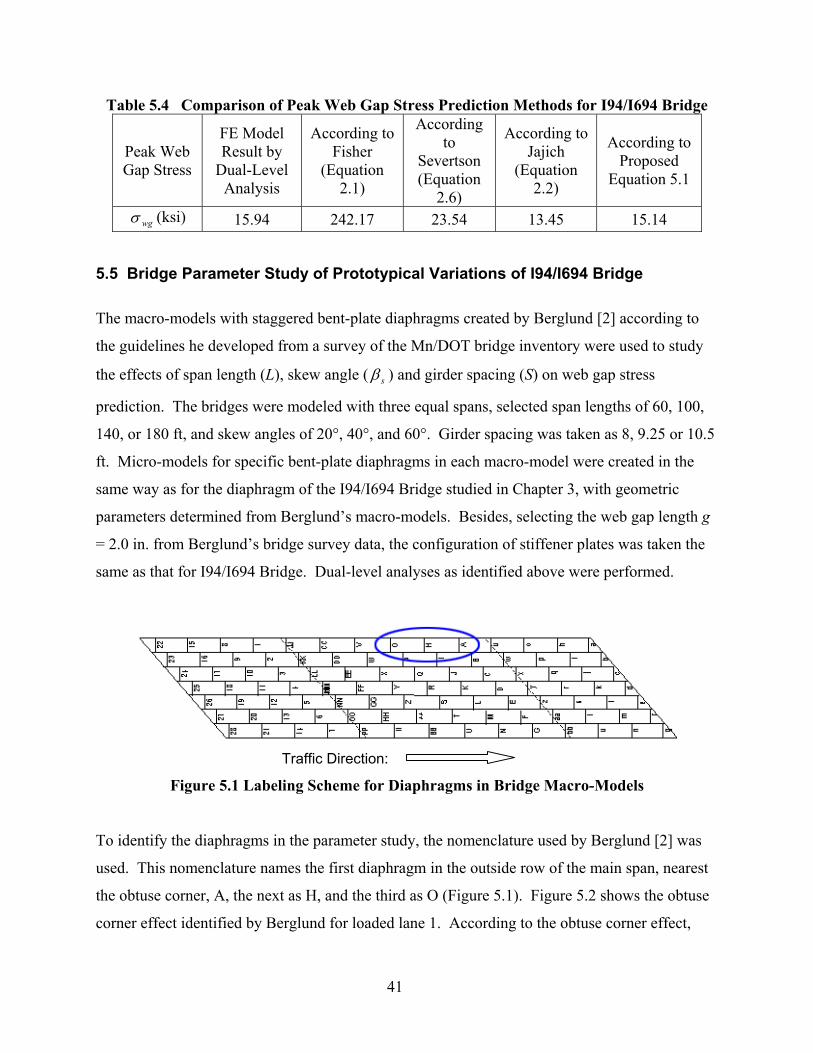
41

Table 5.4 Comparison of Peak Web Gap Stress Prediction Methods for I94/I694 Bridge

Peak Web Gap Stress

FE Model Result by

Dual-Level Analysis

According to Fisher

(Equation 2.1)

According to

Severtson (Equation

2.6)

According to Jajich

(Equation 2.2)

According to Proposed

Equation 5.1

wgσ (ksi) 15.94 242.17 23.54 13.45 15.14

5.5 Bridge Parameter Study of Prototypical Variations of I94/I694 Bridge

The macro-models with staggered bent-plate diaphragms created by Berglund [2] according to

the guidelines he developed from a survey of the Mn/DOT bridge inventory were used to study

the effects of span length (L), skew angle ( sβ ) and girder spacing (S) on web gap stress

prediction. The bridges were modeled with three equal spans, selected span lengths of 60, 100,

140, or 180 ft, and skew angles of 20°, 40°, and 60°. Girder spacing was taken as 8, 9.25 or 10.5

ft. Micro-models for specific bent-plate diaphragms in each macro-model were created in the

same way as for the diaphragm of the I94/I694 Bridge studied in Chapter 3, with geometric

parameters determined from Berglund’s macro-models. Besides, selecting the web gap length g

= 2.0 in. from Berglund’s bridge survey data, the configuration of stiffener plates was taken the

same as that for I94/I694 Bridge. Dual-level analyses as identified above were performed.

Figure 5.1 Labeling Scheme for Diaphragms in Bridge Macro-Models

To identify the diaphragms in the parameter study, the nomenclature used by Berglund [2] was

used. This nomenclature names the first diaphragm in the outside row of the main span, nearest

the obtuse corner, A, the next as H, and the third as O (Figure 5.1). Figure 5.2 shows the obtuse

corner effect identified by Berglund for loaded lane 1. According to the obtuse corner effect,

Traffic Direction:

42

maximum diaphragm differential deflection was typically found at locations in the obtuse

corners of a given loaded lane. Special attention was given to the differential deflections in the

obtuse corners of the main spans, thus diaphragms A, H, O in Figure 5.1 under lane 1 loading of

one 222-kN (50-kip) sand truck were the focus of the study.

Lane 4

Lane 3

Lane 2

Lane 1

122 15 8

223 16 9

324 17 10

425 18 11

526 19 12

627 20 13

728 21 14

Figure 5.2 Lane 1 Loading Obtuse Corner Effect

The coefficient C in Equation 5.2 is defined as )//()2( SC tb ∆+= θθ , with the understanding

that if the value of C can be approximated and lateral deflection δ can be neglected, peak web

gap stress can be easily predicted with Equation 5.2. The calculated values of C for diaphragms

A, H, O with girder spacing S = 10.5 ft and skew angles of 20°, 40°, 60° at different span lengths

are shown in Table 5.5. The results in Table 5.5 show that for span lengths smaller than 180 ft,

the values for C at diaphragms H and O are very close to each other, and are larger than those at

diaphragm A. For span length 180 ft, C values at diaphragm H are approximately between the

values at diaphragms A and O, but the differences are small. Noting that diaphragm A is near

the right pier in the main span, while diaphragms H and O are away from the pier, it is noted that

in the main span, C values are different for diaphragms near the pier and diaphragms away from

the pier. Diaphragm O was not studied for span length 60 because it is also a diaphragm near the

pier on the other end of the main span and it is expected to have similar results as diaphragm A.

For a span length of 180 ft, diaphragms A and H are close to the pier, diaphragm O is away from

the pier and close to the middle location of the main span. C does not change much with

variation of the skew angle except for the case of βs=60° at span length 100 ft compared with

skew angles of 20° and 40°, but if this case is treated as an outlier, it does not influence the

43

general trend. Span length L and diaphragm location relative to the pier are the two major

parameters that affect the values of coefficient C. C decreases with increases in L, and C for

diaphragms away from the pier is larger than that for diaphragms near the pier.

Table 5.5 Coefficient C for Models with Girder Spacing S = 10.5 ft

C at Diaphragm Locations Span Length, L (ft)

Angle of Skew (degree) Diaphragm A Diaphragm H Diaphragm O

60 20 2.92 2.89 60 40 2.89 2.99 60 60 2.83 3.06 100 20 2.21 2.48 2.46 100 40 2.58 2.66 2.65 100 60 1.86 2.17 2.22 140 20 2.31 2.55 2.57 140 40 2.43 2.62 2.64 140 60 2.3 2.65 2.56 180 20 2.03 2.05 2.28 180 40 1.82 2.19 2.33 180 60 1.93 2.1 2.26

The values in Table 5.5 were divided into two series (near the pier and away from the pier), as a

function of span length, and are plotted in Figure 5.3. The following linear trend lines

036.3004.0 +−= LC Equation 5.3(a)

0925.3006.0 +−= LC Equation 5.3(b)

for diaphragms away from (Equation 5.3(a)) and near the pier (Equation 5.3(b)), respectively,

(Figure 5.3) give reasonably accurate estimates for C for bridges with girder spacing of 10.5 ft.

Table 5.6 shows calculated values of C for models with different girder spacing. C does not

change much when girder spacing decreases from 10.5 ft to 9.25 ft. For girder spacing of 8 ft, C

increases a little compared with the larger girder spacing. For the case of L = 100 ft, the result

for a skew angle of 60° is an outlier for the general trend and is ignored. And, for L=100 ft,

values of C at S = 9.25 ft in Table 5.6 are close to the values at S=10.5 ft, sβ = 40° at

corresponding diaphragm locations. In general, the influence of girder spacing on C is

44

insignificant compared with the influence of span length, and Equations 5.3 (a) and 5.3 (b) can

also be used for bridges with girder spacing other than 10.5 ft.

y = -0.004x + 3.036

y = -0.006x + 3.0925

1

1.5

2

2.5

3

3.5

0 20 40 60 80 100 120 140 160 180 200

Main Span Length, L (ft)

Coe

ffic

ient

C C

alcu

late

d fr

om D

ual-l

evel

Ana

lyse

s

Diaphragms Near the Pier Diaphragms Away from the Pier

Linear (Diaphragms Away from the Pier) Linear (Diaphragms Near the Pier)

Figure 5.3 Linear Approximation of C for Diaphragms at Girder Spacing 10.5 ft

Table 5.6 Coefficient C for Models with Skew Angle 60° at Different Girder Spacings S = 10.5 ft S = 9.25 ft S = 8 ft L

(ft) sβ A H O A H O A H O

60 60° 2.83 3.06 2.6 3.03 2.9 3.15 40° 2.58 2.66 2.65 100 60° 1.86 2.17 2.22 2.53 2.65 2.66 2.64 2.75 2.73

140 60° 2.3 2.65 2.56 2.28 2.58 2.57 2.53 2.72 2.73 180 60° 1.93 2.1 2.26 1.94 2.14 2.2 2.1 2.31 2.44

The diaphragm studied in the parameter study for the I94/I694 Bridge is labeled diaphragm 1 in

Figure 5.1, it is located at the west span, and it is near the pier. To find out whether diaphragms

located at end spans or between different girders in the main span have trends for C that differ

from that in Equation 5.3, a model with span length L = 140 ft, girder spacing S =9.25 ft and

skew angle 60° that has similar configuration as the I94/I694 Bridge (L = 138 ft, S =9.25 ft, skew

60°) was selected for study. Values for C were calculated for diaphragms 1, C, 8, X (Figure 5.1)

to compare with diaphragms A and H using dual-level analyses, the results of which are shown

in Figure 5.4. Diaphragms A, 1, C are near the pier, and the values for C at these locations are

45

close to each other. Diaphragms H, 8, X are away from the pier, and the values for C at these

diaphragms are close to each other as well.

L140s925sk60 Model

0

0.5

1

1.5

2

2.5

3

A 1 C H 8 X

Diaphragm Location

Coef

ficie

nt C

Figure 5.4 Values of Coefficient C at Different Diaphragm Locations

This study indicates that it is appropriate to classify the diaphragms in the entire bridge into two

categories: the ones near the pier and those away from the pier. Equations 5.3(a) and 5.3 (b) can

be used to predict C for diaphragms in all spans and between any two girders for bridges having

similar configurations as the model selected in Figure 5.4 (i.e. L = 140 ft, girder spacing S =9.25

ft and skew angle 60°). The predicted values of C using Equations 5.3 (a) and 5.3 (b) for

different span lengths are listed in Table 5.7. The predicted value of C for diaphragm 1 of

I94/I694 bridge using Equation 5.3(a) is 2.265, and this value is consistent with C = 2.25 taken

above in the parameter study of I94/I694 Bridge. The values for C given in Table 5.7 fall

between 2.0 and 2.8, which are larger than C = 2.0, as specified in Jajich’s formula [1], and

smaller than C = 3.5, as shown in Severtson’s formula [3].

In the diaphragm parameter study for the I94/I694 Bridge (section 5.3), it was indicated that C

can be taken as a constant equal to 2.25. While in the bridge parameter study (section 5.4), the

value of C was found to be a function of span length, L, as well as location (i.e., proximity to the

piers). The reason is that the diaphragm parameter study focused on a single span length (L =

46

138 ft) and the diaphragm selected for study is located near the pier. Thus, a mean value for C

equal to 2.25 for the I94/I694 Bridge is appropriate as shown in Table 5.7.

Table 5.7 Prediction of Coefficient C for Bent-Plate Diaphragms

Linear Prediction of C using Equation 5.3 Span Length L (ft) Diaphragms Near the Pier Diaphragms Away from

the Pier 60 2.733 2.796 100 2.493 2.636 140 2.253 2.476 180 2.013 2.316

138 (I94/I694 Bridge) 2.265 2.484

Berglund [2] proposed a single polynomial formula to predict the maximum differential

deflection, ∆, without specifying diaphragm location. The formula for C for diaphragms away

from the piers in Equation 5.3 provides a larger value for C if L exceeds 50 ft, and it is noted

from the dual-level analyses that the maximum ∆ occurred, more often than not, in diaphragms

away from the piers for L larger than 60 ft. Thus, it is assumed that maximum stresses will occur

in diaphragms away from the piers – as long as the other parameters in Equation 5.2 are the

same. For multi-girder steel bridges with staggered bent-plate diaphragms in the Mn/DOT

inventory, the coefficient C can be approximated using the formula for diaphragms away from

the piers (Equation 5.3(a)), and peak web gap stress can be predicted with Equation 5.2 using the

value of ∆/S predicted from Berglund’s formula, assuming that there is evidence that δ can be

neglected.

5.6 Comparison of 50-kip and HS-20 Truck Loadings

The bridge parameter study described above was based on one 222-kN (50-kip) sand truck

loading because the field tests reported by Jajich [1] and Severtson [3] utilized such trucks as

well. The diaphragm parameter study for I94/I694 Bridge has shown that the coefficient C does

not change much under different sweeps of the 50-kip sand truck. The 311-kN (72kip)

AASHTO HS-20 truck (Figure 5.5) has a different axle configuration from the 50-kip sand truck

(Figure 3.6). Berglund [2] reported the diaphragm locations where maximum differential

deflections occurred under HS-20 truck loading of lane 1. These diaphragms, in models with

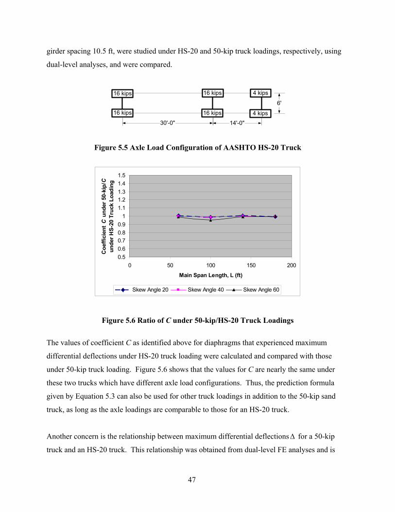
47

girder spacing 10.5 ft, were studied under HS-20 and 50-kip truck loadings, respectively, using

dual-level analyses, and were compared.

16 kips

16 kips

4 kips

4 kips

16 kips

16 kips

30'-0" 14'-0"

6'

Figure 5.5 Axle Load Configuration of AASHTO HS-20 Truck

0.50.60.70.80.9

11.11.21.31.41.5

0 50 100 150 200

Main Span Length, L (ft)

Coe

ffici

ent

C u

nder

50-

kip/

C

unde

r HS-

20 T

ruck

Loa

ding

Skew Angle 20 Skew Angle 40 Skew Angle 60

Figure 5.6 Ratio of C under 50-kip/HS-20 Truck Loadings

The values of coefficient C as identified above for diaphragms that experienced maximum

differential deflections under HS-20 truck loading were calculated and compared with those

under 50-kip truck loading. Figure 5.6 shows that the values for C are nearly the same under

these two trucks which have different axle load configurations. Thus, the prediction formula

given by Equation 5.3 can also be used for other truck loadings in addition to the 50-kip sand

truck, as long as the axle loadings are comparable to those for an HS-20 truck.

Another concern is the relationship between maximum differential deflections ∆ for a 50-kip

truck and an HS-20 truck. This relationship was obtained from dual-level FE analyses and is

48

shown in Figure 5.7. An exponential best-fit curve for the computed data is seen to approximate

∆ under a 50-kip truck satisfactorily if ∆ under an HS-20 truck is given. Berglund [2] gave a

polynomial formula to estimate the value of S/∆ under HS-20 truck loadings. Therefore, with

the exponential equation in Figure 5.7, S/∆ under a 50-kip truck can be also approximated.

y = 3.9321x-0.3282

0

0.2

0.4

0.6

0.8

1

1.2

1.4

0 50 100 150 200

Main Span Length, L (ft)

Max

imum

Diff

eren

tial D

efle

ctio

ns

unde

r 50-

kip

/ und

er H

S-20

Tru

ck

Load

ing

on th

e Ed

ge L

ane

Figure 5.7 Ratio of Maximum Differential Deflections under 50-kip and HS-20 Truck

Loadings

Given the approximation of both C and S/∆ , the peak web gap stress can be estimated easily

using Equation 5.2 for the two types of truck loading. The ratios of peak web gap stresses

calculated from finite element dual-level analyses under the two truck loadings are plotted in

Figure 5.8. The trend observed in Figure 5.8 is very similar to that shown in Figure 5.7, and the

ratio of peak web gap stresses can be approximated with the same equation as the ratio of ∆

under the two truck loadings. This phenomenon is reasonable because C is the same under the

two truck loadings, and according to Equation 5.2, the ratio of peak web gap stress wgσ should

follow the same trend as the ratio of ∆ for the same diaphragm under two truck loadings.

49

0

0.2

0.4

0.6

0.8

1

1.2

1.4

0 50 100 150 200

Main Span Length, L(ft)

Peak

Web

-Gap

Stre

ss u

nder

50-

kip

/ und

er H

S-20

Tru

ck L

oadi

ng

Figure 5.8 Peak Web Gap Stresses, wgσ , under 50-kip and HS-20 Truck Loadings

For span length L = 60 ft, ∆ and wgσ under the 50-kip truck loading are slightly larger than ∆

and wgσ , respectively, under HS-20 loading. The reason is that the span length of 60 ft

approaches the 44 ft total length of an HS-20 truck. Thus, the load transfer distance along the

perpendicular path between pier supports is shorter compared with that for 50-kip truck, and the

pier supports on both ends of the span reduce the differential deflection values.

The management of bridges is usually associated with the largest AASHTO truck configuration,

the HS-20 configuration, rather than a 50-kip sand truck. However, in this and previous studies

on web gap stresses in multi-girder steel bridges, it has been necessary to correlate the stress or

displacement response under these two truck loadings because 50-kip sand trucks were used to

generate the field measurements. Therefore, it is useful to define a decimal scaling factor RL =

kip50−∆ / 20HS−∆ , where kip50−∆ is the maximum differential deflection under 50-kip truck loading,

and 20HS−∆ is the maximum differential deflection under HS-20 truck loading. The exponential

Equation 5.4 from Figure 5.7 can be used for the prediction of RL, the unit for span length L is ft.

3282.09321.3 −⋅= LRL Equation 5.4

50

Given the similarity of Figures 5.7 and 5.8, the same scaling factor can be used for stresses such

that RL ≈ 20HSkip50 / −−wgwg σσ , where kip−50σ is the maximum web gap stress under 50-kip truck

loading, and 20−HSσ is the maximum web gap stress under HS-20 truck loading. Finally, it is

noted that the relations between deflections or stresses for 50-kip and HS-20 truck loadings are

of concern only when considering field measurements made using 50-kip dump trucks.

5.7 Stresses from the Bridge Parameter Study of I94/I694 Bridge

Peak web gap stress is the single bridge response quantity of most concern in this study. Based

on the data from the bridge parameter study (i.e., the dual-level analyses on models that were

prototypical variations of I94/I694 Bridge), maximum differential deflections and peak web gap

stress values were determined for each skew angle at each span length.

Table 5.8 Peak Web Gap Stress Values for Girder Spacing S = 10.5 ft Maximum S/∆

from FE Analyses

Finite Element wgσ (ksi) L

(ft) sβ

(deg.) Value Locat

ion

PredictedS/∆ by

Eq. 2.3 and RL in Eq. 5.4 Value Locat

ion

Predicted wgσ w/o δ,

Eqs.5.2 & 5.3(a) (ksi)

Predictedwgσ with δ from FE

results (ksi)

60 20 0.000771 A 0.000791 7.9 H 16.04 7.35 60 40 0.000814 A 0.000752 7.46 A 15.24 6.80 60 60 0.000658 A 0.000615 10.61 A 12.48 12.37

100 20 0.000687 H 0.000692 9.91 H 13.23 13.66 100 40 0.000587 H 0.000702 6.59 H 13.42 9.39 100 60 0.000733 A 0.000780 25.91 A 14.92 32.04 140 20 0.000531 H 0.000557 8.28 O 10.00 9.66 140 40 0.000587 H 0.000588 7.22 H 10.55 7.83 140 60 0.000627 H 0.000706 10.1 A 12.67 9.49 180 20 0.000405 O 0.000430 5.04 O 7.21 5.95 180 40 0.000460 O 0.000473 4.96 A 7.94 5.48 180 60 0.000537 H 0.000587 6.49 H 9.86 8.91

Table 5.8 shows the maximum values for S/∆ , peak web gap stresses and corresponding

diaphragm locations calculated from bridge models under 50-kip truck loading on lane 1.

Berglund’s (2001) formula (Equation 2.3), together with the correction factor RL proposed by

Equation 5.4 gives good approximations for the maximum S/∆ without specifying the location.

The stress values calculated with the predicted S/∆ , the proposed Equation 5.2 and the

51

coefficient C for diaphragms away from the piers (Equation 5.3), are also listed. It can be seen

that Equation 5.2 in conjunction with Equation 5.3 gives reasonable estimates on peak web gap

stress wgσ in most cases, while in a few cases, it may over predict the stress values with

relatively large errors. The reason is that the lateral deflection δ is larger in some cases

according to the results of finite element analysis, andδ also varies with web gap length and web

thickness. To study the influence ofδ , Equation 2.5 was used for stress prediction, where (2θb +

θt) = C · (∆ /S), C was approximated by Equation 5.3 (a) and S/∆ was predicted using Equations

2.3 & 5.4, δ was taken from the corresponding finite element results for the diaphragms

experienced the maximum deflections, and the results were listed in the last column of Table 5.8.

Table 5.8 shows that web gap lateral deflection δ should be included in conjunction with S/∆

and C in the stress formula to give more reasonable estimates of peak web gap stress, wgσ .

Though the diaphragms that experienced maximum differential deflections are not definitely the

locations where the peak web gap stresses occurred in Table 5.8, the proposed stress prediction

method is still satisfactory if δ is included.

0

5

10

15

20

25

30

0 50 100 150 200

Main Span Length, L (ft)

Peak

Web

-Gap

Stre

ss fo

r G

irder

Spa

cing

10.

5 ft,

(ksi

)

Skew Angle 20 Skew Angle 40 Skew Angle 60

Figure 5.9 Peak Web Gap Stresses wgσ under 50-kip Truck Lane 1 Loading for S = 10.5 ft

Figure 5.9 shows the data for wgσ calculated from finite element analyses in Table 5.8. Ignoring the outlier point at L = 100 ft as indicated above, it is noted that the peak web gap stress wgσ takes a nearly constant value at about 8 ksi, even though the actual value decreases a little with

52

increases in L. Thus, wgσ ≈ 8 ksi can be used as a rough estimate of the peak web gap stress in bent-plate diaphragm bridges in the bridge parameter study with girder spacing S = 10.5 ft. For girder spacing S = 9.25 ft and S = 8 ft, models with skew angle 60° were analyzed and girder

spacing was found to have little influence on the coefficient C in the stress prediction formula

above. A comparison is made in Table 5.9. Peak web gap stresses wgσ calculated from finite

element dual-level analyses were smaller for shorter girder spacing (S), and Equation 5.2 over

predicts peak web gap stress values for S = 9.25 ft and, especially, for S = 8 ft. The reason is that

the lateral deflection δ is larger for smaller girder spacing according to the results of finite

element analysis, andδ also varies with web gap length and web thickness.

To study the influence ofδ , Equation 2.5 was used for stress prediction, where (2θb + θt) = C ·

(∆ /S) and C was approximated by Equation 5.3(a). The ratio for S/∆ was predicted using

Equations 2.3 and 5.4, δ was taken from the FE results for diaphragms that experienced the

maximum deflections, and the results of prediction with δ for different girder spacing are listed

in Table 5.9. Table 5.9 shows that web gap lateral deflection δ should be included in

conjunction with S/∆ and C in the stress formula to give more reasonable estimates of peak

web gap stress, wgσ .

Table 5.9 Comparison of Peak Web Gap Stress for Different Girder Spacings

S = 10.5 ft, wgσ (ksi) S = 9.25 ft, wgσ (ksi) S = 8 ft, wgσ (ksi)

L (ft)

Predicted wgσ w/o δ (ksi),

(Equation 5.2)

FE Result

Prediction with δ from FE results

FE Result

Prediction with δ from FE results

FE Result

Prediction with δ from FE results

60 12.48 10.61 12.37 4.78 7.26 5.08 3.09 100 14.92 25.91 32.04 5.19 7.85 2.01 2.51 140 12.67 10.1 9.49 8.9 9.28 2.99 3.63 180 9.86 6.49 8.91 6.33 7.14 3.34 3.98

Note : Skew Angle sβ = 60°.

So far, no approximate procedure has been determined for the prediction of δ . Consequently,

Equation 5.2 and Equation 5.3 are suggested to be used for multi-girder steel bridges with

53

staggered bent-plate diaphragms in the Mn/DOT inventory, and the lateral deflection δ should be

included if there is evidence that web gap lateral deformation is of importance for a given bridge.

54

Chapter 6 - Parameter Study and Stress Formula Calibration of Prototypical Variations of Plymouth Ave. Bridge

6.1 Overview

This chapter comprises dual-level analyses and stress formula calibration for prototypical

variations of the Plymouth Ave. Bridge in Minneapolis. The modification factor, Rx, developed

by Beukema [3] for the reduction of maximum differential deflections from Berglund’s formula

[2] for bridges with cross-brace diaphragms was further calibrated in this study. In addition,

maximum differential deflection of bridges with a combination railing system (i.e., Type F

barrier plus a raised sidewalk) were calculated and compared with those of bridges with traffic

railing system (i.e., Type J barrier only for the edge rail), and another modification factor, Rd,

was proposed to account for the influence of additional sidewalks on differential deflections.

This chapter discusses the sensitivity of cross-brace diaphragm stress response to prototypical

variations of typical diaphragm and bridge parameters. In the diaphragm parameter study,

properties of the diaphragm and the web gap region (i.e., web gap size, web thickness, girder

flange thickness, differential deflection and deck thickness) of both the macro-model (i.e.,

encompassing the entire bridge) and micro-model (i.e., encompassing a portion of bridge) finite

element representations for the Plymouth Ave. Bridge were independently varied and the

responses of the models were monitored. In the bridge parameter study, macro- and micro-

models for cross-brace diaphragm bridges consistent with Berglund’s guidelines for

proportioning bridge models [2] were created to study the influences of parameters representing

bridge properties (i.e., angle of skew, main span length, and girder spacing) in web gap stress

prediction. The constant coefficient (C) in the stress prediction formula that was proposed in the

study of bent-plate diaphragms evaluated for cross-brace diaphragms, and peak web gap stress

estimates were recommended for cross-brace diaphragms.

55

6.2 Modification Factor for Differential Deflections of Cross-Brace Diaphragms

In previous research by Beukema [3], a modification factor Rx was developed to enable the

application of Berglund’s formula [2] to cross-brace diaphragms. The factor Rx was defined as a

scaling correction factor, relative to a value of unity, for reduction of maximum differential

deflection from Berglund’s formula due to the enhanced stiffness provided by the cross-brace

diaphragms. That is, bpcbxR ∆∆= / , where cb∆ represents the maximum differential deflection in

bridges with cross-brace diaphragms and bp∆ is the maximum differential deflection in bridges

with bent-plate diaphragms, the latter which can be predicted using Berglund’s formula.

Beukema [3] gave a polynomial equation for Rx based upon finite element macro-model analysis

of the bridges in Berglund’s primary parameter study having a girder spacing of 10.5 ft.

Berglund’s bridge survey showed that girder spacing for steel highway bridges generally varied

between 8 ft and 10.5 ft, with no particular trend towards either of these values. To study the

influence of girder spacing on the values of Rx, the finite element models used by Berglund in the

primary parameter study with girders spaced at 8 ft, as well as those in the secondary parameter

study with girders spaced at 9.25 ft, were selected for modification as described below. Only a

few bridge models at girder spacing of 9.25 ft were developed by Berglund in the secondary

study. To get a complete sample of bridge models at all three values for girder spacing (8 ft,

9.25 ft, 10.5 ft), the models needed for girder spacing of 9.25 ft were created in the present

research according to the same guidelines developed by Berglund [2].

To identify the diaphragms in the parameter study, the nomenclature used by Berglund [2] was

used. This nomenclature names the first diaphragm in the outside row of the main span, nearest

the obtuse corner, A, the next as H, and the third as O (Figure 5.1).

The single-line elements representing bent-plate diaphragms in Berglund’s finite element macro-

models [2] were replaced with cross-brace elements in the style of those used in the model of

Plymouth Ave. Bridge. The models with girder spacing of 8 ft and 9.25 ft were each tested, in

both diaphragm configurations, to find the magnitude and location of the maximum diaphragm

differential deflection, as Beukema [3] did in his research for the case of girder spacing S = 10.5

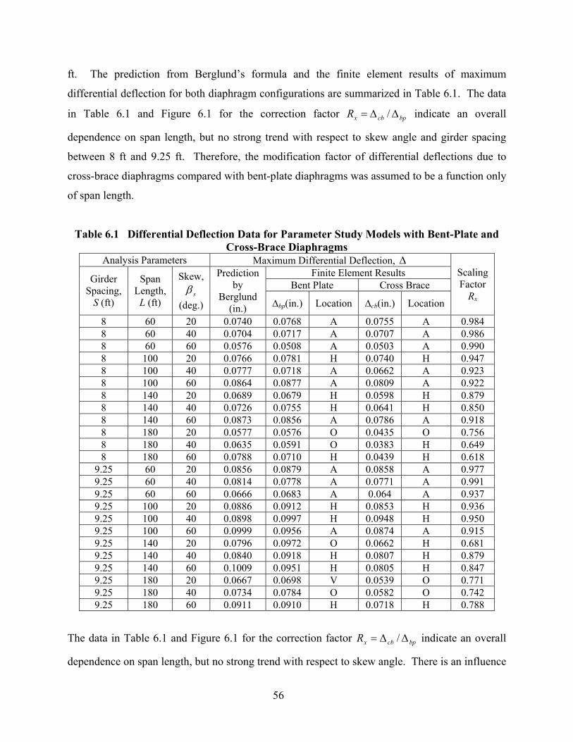
56

ft. The prediction from Berglund’s formula and the finite element results of maximum

differential deflection for both diaphragm configurations are summarized in Table 6.1. The data

in Table 6.1 and Figure 6.1 for the correction factor bpcbxR ∆∆= / indicate an overall

dependence on span length, but no strong trend with respect to skew angle and girder spacing

between 8 ft and 9.25 ft. Therefore, the modification factor of differential deflections due to

cross-brace diaphragms compared with bent-plate diaphragms was assumed to be a function only

of span length.

Table 6.1 Differential Deflection Data for Parameter Study Models with Bent-Plate and Cross-Brace Diaphragms

Analysis Parameters Maximum Differential Deflection, ∆ Finite Element Results

Bent Plate Cross Brace Girder Spacing,

S (ft)

Span Length,

L (ft)

Skew, sβ

(deg.)

Prediction by

Berglund (in.) ∆bp(in.) Location ∆cb(in.) Location

Scaling Factor

Rx

8 60 20 0.0740 0.0768 A 0.0755 A 0.984 8 60 40 0.0704 0.0717 A 0.0707 A 0.986 8 60 60 0.0576 0.0508 A 0.0503 A 0.990 8 100 20 0.0766 0.0781 H 0.0740 H 0.947 8 100 40 0.0777 0.0718 A 0.0662 A 0.923 8 100 60 0.0864 0.0877 A 0.0809 A 0.922 8 140 20 0.0689 0.0679 H 0.0598 H 0.879 8 140 40 0.0726 0.0755 H 0.0641 H 0.850 8 140 60 0.0873 0.0856 A 0.0786 A 0.918 8 180 20 0.0577 0.0576 O 0.0435 O 0.756 8 180 40 0.0635 0.0591 O 0.0383 H 0.649 8 180 60 0.0788 0.0710 H 0.0439 H 0.618

9.25 60 20 0.0856 0.0879 A 0.0858 A 0.977 9.25 60 40 0.0814 0.0778 A 0.0771 A 0.991 9.25 60 60 0.0666 0.0683 A 0.064 A 0.937 9.25 100 20 0.0886 0.0912 H 0.0853 H 0.936 9.25 100 40 0.0898 0.0997 H 0.0948 H 0.950 9.25 100 60 0.0999 0.0956 A 0.0874 A 0.915 9.25 140 20 0.0796 0.0972 O 0.0662 H 0.681 9.25 140 40 0.0840 0.0918 H 0.0807 H 0.879 9.25 140 60 0.1009 0.0951 H 0.0805 H 0.847 9.25 180 20 0.0667 0.0698 V 0.0539 O 0.771 9.25 180 40 0.0734 0.0784 O 0.0582 O 0.742 9.25 180 60 0.0911 0.0910 H 0.0718 H 0.788

The data in Table 6.1 and Figure 6.1 for the correction factor bpcbxR ∆∆= / indicate an overall

dependence on span length, but no strong trend with respect to skew angle. There is an influence

57

on girder spacing between 8 ft and 9.25 ft for bridges with long spans (i.e., 150 ft or more).

Therefore, the modification factor for differential deflections due to cross-brace diaphragms

compared with bent-plate diaphragms can be assumed to be a function of both span length and

girder spacing, or it can be approximated as a function of span length only. Both options were

investigated in the subsequent evaluation, as noted in Figure 6.2 (a), but the differences in Rx for

bridge models with 8-ft and 9.25-ft girder spacing were found to be negligible.

0

0.2

0.4

0.6

0.8

1

1.2

0 50 100 150 200

Main Span Length (ft)

Diff

eren

tial D

efle

ctio

nC

orre

ctio

n Fa

ctor

, Rx

Skew 20 Spacing 8'Skew 40 Spacing 8'Skew 60 Spacing 8'Skew 20 Spacing 9.25'Skew 40 Spacing 9.25'Skew 60 Spacing 9.25'

Figure 6.1 Correction Factor Rx for Maximum Differential Deflection in Cross-Brace

Diaphragms

The data in Table 6.1, combining all data from analysis on bridge models with a girder spacing

of 10.5 ft by Beukema [3], and corresponding trend lines were plotted in Figure 6.2(a). It was

assumed by Beukema that for decreasing span lengths, the difference in load distribution

mechanisms between cross-brace and bent-plate diaphragms would become negligible,

consistent with the indication of the data. It shows that for the cases of girder spacing between 8

ft and 9.25 ft, the trends are similar and can be approximated with a single polynomial as

indicated in Figure 6.2(b). This polynomial has the same form as the one given by Beukema

(Equation 2.7), but values for the constant coefficients B1 and B2 given in Table 6.2 are different.

58

0

0.2

0.4

0.6

0.8

1

1.2

0 50 100 150 200

Main Span Length (ft)

Diff

eren

tial D

efle

ctio

nC

orre

ctio

n Fa

ctor

, Rx

Girder Spacing 10.5' Girder Spacing 8'Girder Spacing 9.25' Poly. (Girder Spacing 10.5')Poly. (Girder Spacing 8') Poly. (Girder Spacing 9.25')

(a) Influence of Girder Spacing

Girder Spacing 8' & 9.25'

y = -1.038E-05x2 + 3.232E-04x + 1.000E+00

0

0.2

0.4

0.6

0.8

1

1.2

0 50 100 150 200Main Span Length (ft)

Diff

eren

tial D

efle

ctio

nC

orre

ctio

n Fa

ctor

,Rx

Correction Factor Poly. (Correction Factor)

(b) Unified Correction Factor

Figure 6.2 Modification Factor Rx for the Prediction of Maximum Differential Deflection in

Cross-Brace Diaphragms

For girder spacing 10.5 ft, the constants in Table 2.2 proposed by Beukema should be used.

Interpolation is recommended if the girder spacing is between 9.25 ft and 10.5 ft. Equation 2.7

gives a general form for the correction factor Rx that can be used for the prediction of maximum

differential deflections in all bridges with cross-brace diaphragms in Mn/DOT inventory.

59

Table 6.2 Constants in Polynomial Equation 2.7 for Girder Spacing Between 8 ft and 9.25 ft

Constants Dimension of L B1 B2 ft -1.038E-05 3.232E-04 in. -7.209E-08 2.694E-05 m -1.117E-04 1.060E-03

6.3 Comparison of Maximum Differential Deflections for Bridges with Additional

Sidewalk Railing and Type J-Rail

A traffic railing system (J-rail) was used in the I94/I694 Bridge and the models studied earlier

(Figure 6.3(a)), while in the Plymouth Ave. Bridge, a raised sidewalk was used in the walkway

area and a Type F barrier was used for protection (Figure 6.3(b)) [21]. The addition of a

concrete sidewalk may influence the susceptibility of diaphragms to distortional fatigue.

(a) J-rail (b) Sidewalk & F-rail Barrier

Figure 6.3 Typical Bridge Cross Sections Showing Two General Classes of Bridge Railings

In the macro-models with bent-plate diaphragms for the bridge parameter study, single-line

frame elements representing the J-rail were replaced with shell elements connected on both sides

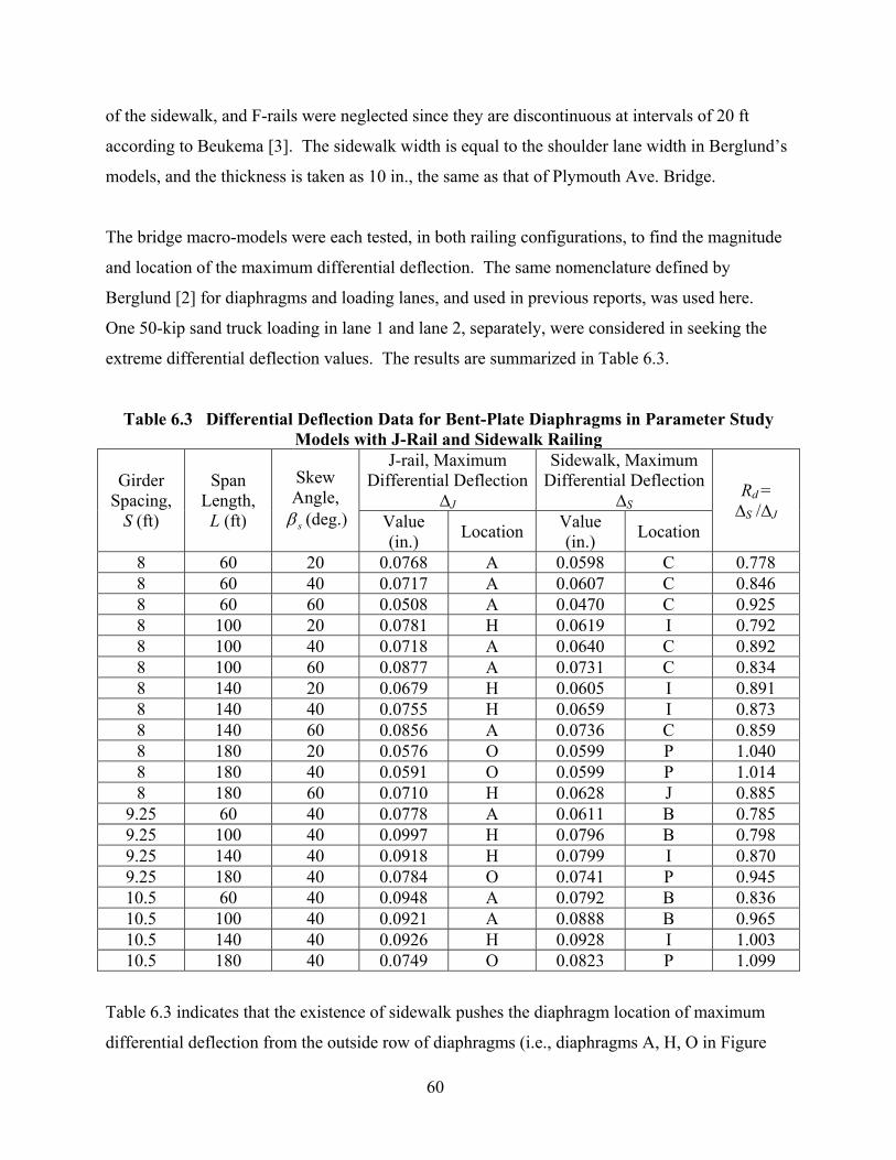
60

of the sidewalk, and F-rails were neglected since they are discontinuous at intervals of 20 ft

according to Beukema [3]. The sidewalk width is equal to the shoulder lane width in Berglund’s

models, and the thickness is taken as 10 in., the same as that of Plymouth Ave. Bridge.

The bridge macro-models were each tested, in both railing configurations, to find the magnitude

and location of the maximum differential deflection. The same nomenclature defined by

Berglund [2] for diaphragms and loading lanes, and used in previous reports, was used here.

One 50-kip sand truck loading in lane 1 and lane 2, separately, were considered in seeking the

extreme differential deflection values. The results are summarized in Table 6.3.

Table 6.3 Differential Deflection Data for Bent-Plate Diaphragms in Parameter Study Models with J-Rail and Sidewalk Railing

J-rail, Maximum Differential Deflection

∆J

Sidewalk, Maximum Differential Deflection

∆S Girder

Spacing, S (ft)

Span Length, L (ft)

Skew Angle,

sβ (deg.) Value (in.) Location Value

(in.) Location

Rd = ∆S /∆J

8 60 20 0.0768 A 0.0598 C 0.778 8 60 40 0.0717 A 0.0607 C 0.846 8 60 60 0.0508 A 0.0470 C 0.925 8 100 20 0.0781 H 0.0619 I 0.792 8 100 40 0.0718 A 0.0640 C 0.892 8 100 60 0.0877 A 0.0731 C 0.834 8 140 20 0.0679 H 0.0605 I 0.891 8 140 40 0.0755 H 0.0659 I 0.873 8 140 60 0.0856 A 0.0736 C 0.859 8 180 20 0.0576 O 0.0599 P 1.040 8 180 40 0.0591 O 0.0599 P 1.014 8 180 60 0.0710 H 0.0628 J 0.885

9.25 60 40 0.0778 A 0.0611 B 0.785 9.25 100 40 0.0997 H 0.0796 B 0.798 9.25 140 40 0.0918 H 0.0799 I 0.870 9.25 180 40 0.0784 O 0.0741 P 0.945 10.5 60 40 0.0948 A 0.0792 B 0.836 10.5 100 40 0.0921 A 0.0888 B 0.965 10.5 140 40 0.0926 H 0.0928 I 1.003 10.5 180 40 0.0749 O 0.0823 P 1.099

Table 6.3 indicates that the existence of sidewalk pushes the diaphragm location of maximum

differential deflection from the outside row of diaphragms (i.e., diaphragms A, H, O in Figure

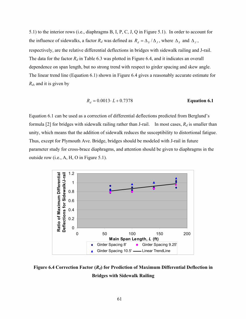
61

5.1) to the interior rows (i.e., diaphragms B, I, P, C, J, Q in Figure 5.1). In order to account for

the influence of sidewalks, a factor Rd was defined as JSdR ∆∆= / , where S∆ and J∆ ,

respectively, are the relative differential deflections in bridges with sidewalk railing and J-rail.

The data for the factor Rd in Table 6.3 was plotted in Figure 6.4, and it indicates an overall

dependence on span length, but no strong trend with respect to girder spacing and skew angle.

The linear trend line (Equation 6.1) shown in Figure 6.4 gives a reasonably accurate estimate for

Rd, and it is given by

7378.00013.0 +⋅= LRd Equation 6.1

Equation 6.1 can be used as a correction of differential deflections predicted from Berglund’s

formula [2] for bridges with sidewalk railing rather than J-rail. In most cases, Rd is smaller than

unity, which means that the addition of sidewalk reduces the susceptibility to distortional fatigue.

Thus, except for Plymouth Ave. Bridge, bridges should be modeled with J-rail in future

parameter study for cross-brace diaphragms, and attention should be given to diaphragms in the

outside row (i.e., A, H, O in Figure 5.1).

0

0.2

0.4

0.6

0.8

1

1.2

0 50 100 150 200Main Span Length, L (ft)

Rat

io o

f Max

imum

Diff

eren

tial

Def

lect

ions

for S

idew

alk/

J-ra

il

Girder Spacing 8' Girder Spacing 9.25'Girder Spacing 10.5' Linear TrendLine

Figure 6.4 Correction Factor (Rd) for Prediction of Maximum Differential Deflection in

Bridges with Sidewalk Railing

62

6.4 Diaphragm Parameter Study for Plymouth Ave. Bridge

In previous research on the I94/I694 Bridge, a diaphragm parameter study was performed with

the calibrated macro- models (i.e., encompassing the entire bridge) and micro-models (i.e.,

encompassing a portion of bridge) described in Chapter 3 to study the effects of typical

diaphragm parameters on peak web gap stress. A similar parameter study was performed on the

Plymouth Ave. Bridge in this document with the calibrated macro- and micro-models described

in Chapter 4. The parameters varied here include web gap length, web thickness, deck thickness,

girder flange thickness, and diaphragm differential deflection. The values of the varied

parameters and the corresponding responses (i.e., peak web gap stress wgσ and web gap

deformations θt, θb, δ) are listed in Table 6.4, and the values contained in the original model (i.e.,

the model that best represents the Plymouth Ave. Bridge) are also noted as “original” in the first

column. The corresponding differential deflections calculated from the macro-model of

Plymouth Ave. Bridge for varied web thickness, flange thickness and deck thickness are listed in

the last column named “note” of Table 6.4.

The ranges of values for web thickness, deck thickness and girder flange thickness were selected

based upon the ranges for these parameters found in the analysis of the Mn/DOT bridge

inventory by Berglund [2]. The web gap lengths were selected to represent the range of lengths

found in Mn/DOT bridge inventory as well as the reports of other researchers by Severtson [3].

The differential deflection was varied by applying the truck sweeps described by Severtson on

the macro-model of Plymouth Ave. Bridge.

Dual-level analyses were employed and more parameters were studied in this research compared

with Severtson’s parameter study [3], which was based upon a single micro-model of the

diaphragm region (and no macro-model of the bridge). A similar trend was observed for the

variations of web gap rotations (θt and θb) and lateral deflection (δ) with the variations of

parameters as identified by Severtson, though the magnitudes of diaphragm responses obtained

are different from Severtson’s reported results. From the results of the parameter study shown in

Table 6.4, it can be seen that all of the parameters studied have an impact on the web gap stress.

63

It can also be noted that the values for both rotations (θt, θb) and the lateral deflection of the web

gap (δ) are affected by the variation of these parameters.

Table 6.4 Diaphragm Parameters Studied and FE Model Results for the Plymouth Ave. Bridge

Parameter Changed

Value (in.) wgσ (ksi) tθ bθ δ (in.) Note

g 1.7 6.39 0.000446 0.00025 -0.00017 g 2 7.44 0.000438 0.000253 -0.00012 g 2.3 8.4 0.000442 0.000256 -0.00005

Original g 2.5 8.23 0.000441 0.000258 0 g 2.7 9.75 0.00044 0.00026 0.00006 g 3 10.73 0.000439 0.000263 0.00015 g 3.3 11.44 0.000438 0.000265 0.00025 tw 0.4375 17.43 0.000462 0.000265 0.00082 ∆ =0.0397in. tw 0.5 11.74 0.000448 0.000259 0.00033 ∆ =0.0392in.

Original tw 0.5625 8.23 0.000441 0.000258 0 ∆ =0.0388in. tw 0.625 5.76 0.000431 0.000254 -0.00021 ∆ =0.0384in. tw 0.75 3.04 0.000416 0.000253 -0.00046 ∆ =0.0377in.

Original ∆ 0.03882 8.23 0.000441 0.000258 0 ∆ 0.02591 7.29 0.000327 0.000196 0.00006 ∆ 0.03394 7.43 0.000333 0.000233 0.00006 ∆ 0.02128 5.34 0.000213 0.000145 0.0001 ∆ 0.01837 4.9 0.000184 0.000126 0.000116

Different Loading Cases

td 8 8.59 0.00049 0.000279 -0.000037 ∆ =0.0426in.Original td 9 8.23 0.000441 0.000258 0 ∆ =0.0388in.

td 10 7.66 0.000397 0.000235 0.0000248 ∆ =0.0355in. tf 0.375 4.81 0.000137 0.000178 0.00021 ∆ =0.0241in. tf 0.5 7.29 0.000372 0.000318 0.00005 ∆ =0.0450in. tf 0.65 6.87 0.000357 0.000266 0.00003 ∆ =0.0383in.

Original tf 1.125 8.23 0.000441 0.000258 0 ∆ =0.0388in. tf 2 10.01 0.000425 0.000218 0.0002 ∆ =0.0349in. tf 2.5 10.21 0.000413 0.000202 0.00026 ∆ =0.0335in.

6.5 Calibration of Stress Prediction Equation for Plymouth Ave. Bridge

After dual-level analysis of the Plymouth Ave. Bridge in Chapter 4, the mechanism of

distortional stress was found to be different from those assumed by Jajich [1] and Severtson

[3]. The web gap experienced both top and bottom rotations and small amounts of out-of-

plane deflection, and this fact suggests that the stress formulas proposed by Jajich and

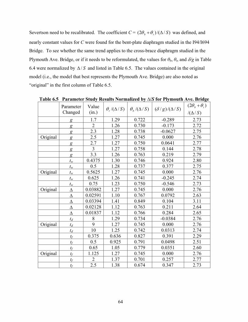
64

Severtson need to be recalibrated. The coefficient C = )//()2( Stb ∆+θθ was defined, and

nearly constant values for C were found for the bent-plate diaphragm studied in the I94/I694

Bridge. To see whether the same trend applies to the cross-brace diaphragm studied in the

Plymouth Ave. Bridge, or if it needs to be reformulated, the values for θb, θt, and δ/g in Table

6.4 were normalized by S/∆ and listed in Table 6.5. The values contained in the original

model (i.e., the model that best represents the Plymouth Ave. Bridge) are also noted as

“original” in the first column of Table 6.5.

Table 6.5 Parameter Study Results Normalized by ∆/S for Plymouth Ave. Bridge

Parameter Changed

Value (in.)

)//( St ∆θ )//( Sb ∆θ )//()/( Sg ∆δ )//(

)2(S

tb

∆+θθ

g 1.7 1.29 0.722 -0.289 2.73 g 2 1.26 0.730 -0.173 2.72 g 2.3 1.28 0.738 -0.0627 2.75

Original g 2.5 1.27 0.745 0.000 2.76 g 2.7 1.27 0.750 0.0641 2.77 g 3 1.27 0.758 0.144 2.78 g 3.3 1.26 0.763 0.219 2.79 tw 0.4375 1.30 0.746 0.924 2.80 tw 0.5 1.28 0.737 0.377 2.75

Original tw 0.5625 1.27 0.745 0.000 2.76 tw 0.625 1.26 0.741 -0.245 2.74 tw 0.75 1.23 0.750 -0.546 2.73

Original ∆ 0.03882 1.27 0.745 0.000 2.76 ∆ 0.02591 1.10 0.767 0.0792 2.63 ∆ 0.03394 1.41 0.849 0.104 3.11 ∆ 0.02128 1.12 0.763 0.211 2.64 ∆ 0.01837 1.12 0.766 0.284 2.65 td 8 1.29 0.734 -0.0384 2.76

Original td 9 1.27 0.745 0.000 2.76 td 10 1.25 0.742 0.0313 2.74 tf 0.375 0.636 0.827 0.391 2.29 tf 0.5 0.925 0.791 0.0498 2.51 tf 0.65 1.05 0.779 0.0351 2.60

Original tf 1.125 1.27 0.745 0.000 2.76 tf 2 1.37 0.701 0.257 2.77 tf 2.5 1.38 0.674 0.347 2.73

65

From Table 6.5 it can be seen that for the Plymouth Avenue Bridge, as was found before for the

I94/I694 Bridge, the values for )//()2( Stb ∆+θθ are fairly consistent for all diaphragm

parameters that were varied. In fact, )//()2( Stb ∆+θθ is much more consistent than either

)//( Sb ∆θ or )//( St ∆θ , while there is no immediately obvious trend for )//()/( Sg ∆δ . By

averaging, a constant value C=2.75 was selected for the cross-brace diaphragm studied here.

With the selected coefficient C = )//()2( Stb ∆+θθ = 2.75, plus the lateral deflection δ and the

differential deflection ∆ recorded in the analysis, the web gap stress can be predicted using the

general stress formula proposed in previous tasks. A comparison for prediction including and

neglecting δ are shown in Table 6.6. The values contained in the original model (i.e., the model

that best represents the Plymouth Ave. Bridge) are also noted as “original” in the first column.

The results in Table 6.6 indicate that neglecting δ for varying values of ∆ and td does not

significantly reduce the accuracy of the stress prediction equation in many cases. However, in

some cases, varying tw and g, and neglecting δ , causes the web gap stress prediction to have an

inverse relationship with the finite element model stresses. And, for larger values of g and tf, and

smaller values of tw, with respect to those used in the original model, the web gap stress formula

(Equation 5.2) may under predict the peak web gap stress. Yet, in the Plymouth Ave. Bridge,

which was monitored by Severtson [3], no significant lateral deflection δ of the web gap region

was observed. Therefore, lacking a simple means to predict δ with reasonable accuracy, it is

recommended that δ be neglected in the stress prediction equation, especially in view of the

lack of field data supporting the presence of non-zero lateral deflections δ.

Using the selected value for C (i.e., C = )//()2( Stb ∆+θθ = 2.75), and neglecting the effect of δ ,

leads to the proposed peak web gap stress prediction as given in Equation 6.2.

∆

=

SgtE w

wg 75.2σ Equation 6.2

Equation 6.2 can be used for cross-brace diaphragms similar to the diaphragm studied and in

bridges with similar geometric configuration as the Plymouth Ave. Bridge. The influence of the

66

principal bridge parameters (i.e., span length, skew angle, and girder spacing) on the prediction

of web gap stresses for cross-brace diaphragms is discussed in the following.

Table 6.6 Comparison of Prediction Equation with and without δ for the Cross-Brace Diaphragm in Plymouth Ave. Bridge

FE Model Prediction w/δ

Prediction w/o δ

(C=2.75) Parameter Changed Value (in.)

wgσ (ksi) wgσ (ksi) wgσ (ksi) g 1.7 6.39 6.27 9.15 g 2 7.44 6.31 7.77 g 2.3 8.4 6.30 6.76

Original g 2.5 8.23 6.22 6.22 g 2.7 9.75 6.16 5.76 g 3 10.73 6.00 5.18 g 3.3 11.44 5.84 4.71 tw 0.4375 17.43 9.95 4.95 tw 0.5 11.74 7.89 5.59

Original tw 0.5625 8.23 6.22 6.22 tw 0.625 5.76 5.01 6.84 tw 0.75 3.04 3.25 8.06

Original ∆ 0.03882 8.23 6.22 6.22 ∆ 0.02591 7.29 5.91 5.44 ∆ 0.03394 7.43 4.62 4.15 ∆ 0.02128 5.34 4.19 3.41 ∆ 0.01837 4.9 3.85 2.94 td 8 8.59 6.53 6.82

Original td 9 8.23 6.22 6.22 td 10 7.66 5.88 5.69 tf 0.375 4.81 5.50 3.86 tf 0.5 7.29 7.59 7.20 tf 0.65 6.87 6.36 6.13

Original tf 1.125 8.23 6.22 6.22 tf 2 10.01 7.15 5.59 tf 2.5 10.21 7.41 5.37

6.6 Bridge Parameter Study of Prototypical Variations of Plymouth Ave. Bridge

As discussed earlier, the single-line elements representing bent-plate diaphragms in macro-

models by Berglund’s guidelines [2] were replaced with cross-brace elements in the style of

67

those used in the model of Plymouth Ave. Bridge. The bridges were modeled with three equal

spans, and the span lengths were selected as 60, 100, 140, or 180 ft; skew angles of 20°, 40°, and

60° were considered; and girder spacing was taken as 8, 9.25 or 10.5 ft. To study the effects of

span length (L), skew angle ( sβ ) and girder spacing (S) on web gap stress prediction, micro-

models for specific cross-brace diaphragms in each macro-model were created in the same way

as for the diaphragm studied in Plymouth Ave. Bridge, with geometric parameters determined

from Berglund’s macro-models. Besides selecting the web gap length g = 2.0 in. from

Berglund’s bridge survey data, the configuration of stiffener plates and cross-brace sections was

taken the same as that of Plymouth Ave. Bridge. The same nomenclature by Berglund as shown

in Chapter 5 was used (Figure 5.1). Special attention was given to the differential deflections in

the obtuse corners of the main spans, thus diaphragms A, H, O under lane 1 loading of one 222-

kN (50-kip) sand truck were the focus of the study. Dual-level analyses as identified previously

were performed.

The Plymouth Ave. Bridge has five spans, features cross-brace diaphragms with an angle-plate

cross section 4"×4"×5/16", and it was designed with lateral wind bracing in spans 2-4 between

interior girders. To verify the modeling guidelines above, the importance of number of spans,

diaphragm cross-sectional area and addition of lateral wind bracing was investigated. The bridge

with L = 140 ft, S = 9.25 ft, and °= 40sβ was selected and varied. This bridge was chosen, in

part, since it has similar geometric configuration as the span studied in Plymouth Ave. Bridge (L

= 156.69 ft, S = 9.33 ft, and °= 5.45sβ ).

The calculated differential deflection ∆, coefficient )//()2( SC tb ∆+= θθ , and web gap stress

wgσ for diaphragms A, H, O are listed in Table 6.7. The first row of Table 6.7 shows the results

for the original model created using the guidelines described in the previous paragraph. The

maximum differential deflections are shown in boldfaced text. It was found that both maximum

differential deflection and peak web gap stress decreased approximately 15% when the number

of bridge spans increased from three to five, which means that bridges with three spans appear to

be more susceptible to web gap distortion. The increase in diaphragm member cross section size

for the cross-brace diaphragms has insignificant influence on the values of ∆, C, and wgσ . The

68

addition of lateral wind bracing between interior girders in the model having five spans caused a

negligible decrease on both ∆ and wgσ . Thus, it is reasonable to consider bridges having three

spans in the bridge parameter study, as in Chapter 5, and use the same configuration for cross-

brace diaphragms as those of Plymouth Ave. Bridge. No lateral wind bracing is needed for the

FE analyses.

Table 6.7 Dual-Level Analyses Results for Plymouth Ave. Bridge using Various

Models (L=140, S=9.25, and βs =40°) Diaphragm A Diaphragm H Diaphragm O

Model Configuration ∆ (in.) C wgσ

(ksi) ∆ (in.) C wgσ

(ksi) ∆ (in.) C wgσ

(ksi) 3 Spans, No

Lateral Bracing,

4"×4"×5/16" Cross Section

0.0520 2.19 11.83 0.0640 2.53 8.52 0.0591 2.55 8.24

3 Spans, No Lateral

Bracing, 4"×4"×1/2"

Cross Section

0.0514 2.24 12.31 0.0633 2.56 8.83 0.0581 2.58 8.4

3 Spans, No Lateral

Bracing, 4"×4"×5/8"

Cross Section

0.0511 2.26 12.44 0.0629 2.57 8.73 0.0576 2.58 8.42

5 Spans, No Lateral

Bracing, 4"×4"×5/16" Cross Section

0.0438 2.19 10.3 0.0591 2.52 8.12 0.0610 2.55 8.31

5 Spans, With Lateral

Bracing, 4"×4"×5/16" Cross Section

0.0434 2.2 10.28 0.0585 2.53 8.01 0.0597 2.54 8.15

If the value of C can be approximated, and lateral deflection δ can be neglected, peak web gap

stress can be easily predicted with the web gap stress formula (Equation 5.2). Figure 6.5 shows

the calculated values of C for cross-brace diaphragms A, H and O in models with L = 140 ft, S =

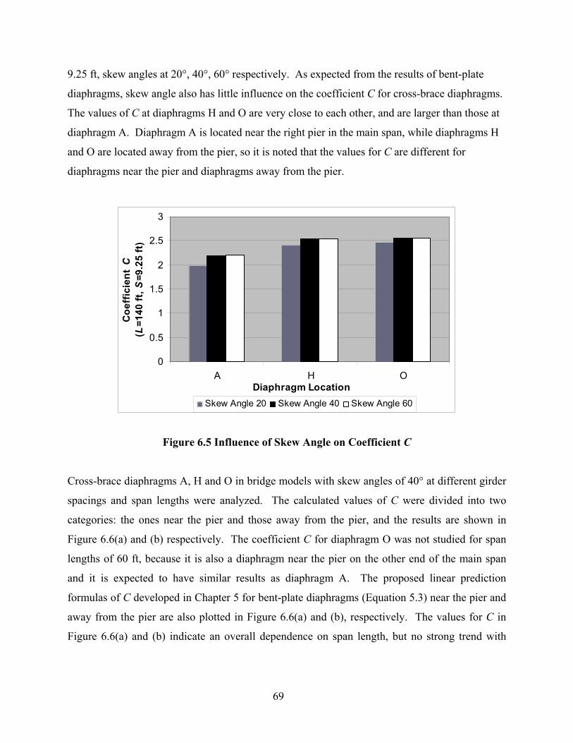
69

9.25 ft, skew angles at 20°, 40°, 60° respectively. As expected from the results of bent-plate

diaphragms, skew angle also has little influence on the coefficient C for cross-brace diaphragms.

The values of C at diaphragms H and O are very close to each other, and are larger than those at

diaphragm A. Diaphragm A is located near the right pier in the main span, while diaphragms H

and O are located away from the pier, so it is noted that the values for C are different for

diaphragms near the pier and diaphragms away from the pier.

0

0.5

1

1.5

2

2.5

3

A H ODiaphragm Location

Coe

ffic

ient

C

(L=1

40 ft

, S=9

.25

ft)

Skew Angle 20 Skew Angle 40 Skew Angle 60

Figure 6.5 Influence of Skew Angle on Coefficient C

Cross-brace diaphragms A, H and O in bridge models with skew angles of 40° at different girder

spacings and span lengths were analyzed. The calculated values of C were divided into two

categories: the ones near the pier and those away from the pier, and the results are shown in

Figure 6.6(a) and (b) respectively. The coefficient C for diaphragm O was not studied for span

lengths of 60 ft, because it is also a diaphragm near the pier on the other end of the main span

and it is expected to have similar results as diaphragm A. The proposed linear prediction

formulas of C developed in Chapter 5 for bent-plate diaphragms (Equation 5.3) near the pier and

away from the pier are also plotted in Figure 6.6(a) and (b), respectively. The values for C in

Figure 6.6(a) and (b) indicate an overall dependence on span length, but no strong trend with

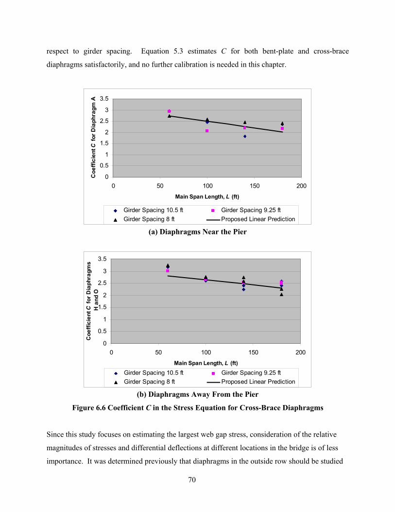
70

respect to girder spacing. Equation 5.3 estimates C for both bent-plate and cross-brace

diaphragms satisfactorily, and no further calibration is needed in this chapter.

0

0.5

1

1.5

2

2.5

3

3.5

0 50 100 150 200

Main Span Length, L (ft)

Coe

ffici

ent C

for D

iaph

ragm

A

Girder Spacing 10.5 ft Girder Spacing 9.25 ftGirder Spacing 8 ft Proposed Linear Prediction

(a) Diaphragms Near the Pier

0

0.5

1

1.5

2

2.5

3

3.5

0 50 100 150 200

Main Span Length, L (ft)

Coe

ffici

ent C

for D

iaph

ragm

s H

and

O

Girder Spacing 10.5 ft Girder Spacing 9.25 ftGirder Spacing 8 ft Proposed Linear Prediction

(b) Diaphragms Away From the Pier

Figure 6.6 Coefficient C in the Stress Equation for Cross-Brace Diaphragms

Since this study focuses on estimating the largest web gap stress, consideration of the relative

magnitudes of stresses and differential deflections at different locations in the bridge is of less

importance. It was determined previously that diaphragms in the outside row should be studied

71

for the purpose of estimating peak web gap stress, so Equation 5.3 was applied to the Plymouth

Ave. Bridge for this purpose. Substituting L = 156.69 ft of span 4 in the Plymouth Ave. Bridge

into Equation 5.3(a) gives C = 2.41 for diaphragms away from the pier in the outside row (i.e., H

and O). The value is smaller than C = 2.75 proposed in Equation 6.2 after the diaphragm

parameter study, the reasons for this deviation are: The diaphragm studied in the Plymouth Ave.

Bridge is not located in the outside row where Equation 5.3 was based on and it did not

experience the maximum differential deflection. This diaphragm corresponds to designation J

according to the labeling scheme (Figure 6.7) and it was modeled for study previously because

the largest peak web gap stress was measured on this diaphragm during field truck testing by

Severtson [3]. In fact, diaphragm H in span 4 of the Plymouth Ave. Bridge (Figure 6.7) was also

instrumented by Severtson and it experienced larger differential deflection than did diaphragm J.

To make a comparison, diaphragm H in Figure 6.7 was also modeled and peak web gap stress

was calculated.

Figure 6.7 Framing Plan of Plymouth Ave. Spans 4 and 5 Highlighting

Diaphragms A, H, O and J

The Plymouth Ave. Bridge features sidewalk railing, so the prediction of maximum differential

deflection ∆ should consider the modification factor Rd for sidewalk railing in Equation 6.1 in

addition to Rx for cross-brace diaphragms in Equation 2.7 and RL for 50-kip truck loading in

Equation 5.4. The value for ∆ predicted from Berglund’s Equation 6.2 was modified using these

three factors for the Plymouth Ave. Bridge, and peak web gap stress wgσ was estimated with the

predicted values for C and ∆.

DiaphragmJ

Traffic Direction

72

The results in Table 6.8 indicate that the proposed formulas give satisfactory estimates for both

maximum differential deflection and peak web gap stress though the location of maximum

differential deflection is not the location where largest web gap stress occurred in this case, and

values of C for diaphragm H from finite element calculation was consistent with the linear

prediction from Equation 5.3. Thus, the various prediction formulas give reasonably accurate

estimates of bridge response to truck loading. Detailed procedures for estimating maximum

differential deflection and peak web gap stress in the Plymouth Ave. Bridge are discussed in the

Appendix.

Table 6.8 Calculation Results for Diaphragms H and J of Plymouth Ave. Bridge

Finite Element Result Predicted Value Loading Diaphragm ∆ (in.) wgσ (ksi) C C ∆ (in.) wgσ (ksi) Lane 1 H 0.0459 7.89 2.44 Lane 2 H 0.0391 6.8 2.48 Lane 2 J 0.0388 8.23 2.76

2.41 0.048 6.74

6.7 Stresses from the Bridge Parameter Study of Plymouth Ave. Bridge

Peak web gap stress values are the single bridge response values of greatest concern in this

study. Based on the data from the bridge parameter study (i.e., the dual-level analyses on models

that were prototypical variations of Plymouth Ave. Bridge), maximum differential deflections

and peak web gap stress values on diaphragms were found at each span length.

Table 6.9 shows the maximum values for S/∆ , peak web gap stresses and corresponding

diaphragm locations calculated from bridge models under 50-kip truck loading on lane 1.

Berglund’s formula [2] (Equation 2.3), together with the correction factors Rx for cross-brace

diaphragms (Equation 2.7) and RL for 50-kip truck loading (Equation 5.4) gives good

approximations for the maximum S/∆ without specifying the location. The stress values

calculated with 1) the predicted S/∆ , 2) the suggested stress formula (Equation 5.2) and 3) the

coefficient C for diaphragms away from the pier in Equation 5.3 (a) were also listed. It can be

seen that for smaller values for girder spacing (i.e., 9.25 ft and 8 ft), the differences between

predictions and FE results of stresses are not negligible. Since the web gap lateral deflection δ

73

was neglected in the derivation of Equation 5.2, the impact of δ on peak web gap stress may

account for this deviation.

Table 6.9 Peak Web Gap Stress Values for Cross-Brace Diaphragms ( sβ = 40°)

Maximum S/∆ from FE Analyses

Finite Element wgσ (ksi)

S (ft) L (ft)

Value Location

PredictedS/∆

Value Location

Predictedwgσ (ksi)

w/o δ (Equation

5.2)

Predictedwgσ (ksi)

with δ from FE results

8 60 0.00082 A 0.000738 9.68 A 14.97 9.49 8 100 0.000588 A 0.000652 5.85 A 12.46 7.51 8 140 0.000546 H 0.000495 6.61 A 8.88 8.07 8 180 0.000334 H 0.000341 12.41 O 5.73 17.16

9.25 60 0.000737 H 0.000738 10.69 H 14.97 10.82 9.25 100 0.000664 H 0.000652 7.35 A 12.46 6.90 9.25 140 0.000577 H 0.000495 11.83 A 8.88 14.98 9.25 180 0.000401 O 0.000341 5.91 O 5.73 4.90 10.5 60 0.000792 A 0.000724 11.16 A 14.68 8.52 10.5 100 0.000616 H 0.000605 7.69 H 11.56 8.68 10.5 140 0.000435 H 0.00041 9.04 A 7.36 14.46 10.5 180 0.000252 H 0.000223 5.49 A 3.75 5.97

To study the influence of δ, Equation 2.5 was used for stress prediction, where (2θb + θt) was

approximated as C · (∆ /S), C was obtained from Equation 5.3 (a), S/∆ was predicted as

described above and listed in Table 6.9, and δ was taken from the corresponding finite element

results for the diaphragms experienced the maximum deflections. The results are listed in the

last column of Table 6.9 which shows that web gap lateral deflection δ should be included in

conjunction with S/∆ and C in the stress formula to give more reasonable estimates of peak

web gap stress, wgσ . Though the diaphragms that experienced maximum differential

deflections are not necessarily the locations where the peak web gap stresses for the bridges

represented in Table 6.9, the proposed stress prediction method is satisfactory if lateral deflection

δ is included for those cases in which lateral deflection is not negligible.

So far, no obvious procedure has been determined for the efficient prediction of δ , and more

research, including field tests and finite element analyses, appears to be required to adequately

characterize the magnitude of lateral deflection δ for the distortional fatigue problem.

Consequently, the procedure identified above is suggested for assessment of distortional fatigue

74

in multi-girder steel bridges with staggered cross-brace diaphragms in the Mn/DOT inventory.

The lateral deflection δ should be included if there is evidence that web gap lateral deformation

is of importance for a given bridge.

75

Chapter 7 - Discussion of Lateral Deflection

7.1 Overview

This chapter discusses the influence of lateral deflection on the out-of-plane distortional stress in

web gaps of multi-girder steel bridges on skew supports. While this phenomenon was not

formally included in the initial scope of study, it is closely related to the discussion contained in

Chapters 5 and 6. Thus, this chapter represents a preliminary analytical effort conducted to help

understand the role of lateral deflection on the mechanism of out-of-plane distortional stress. It

is noted, however, that before this effort can generate a credible procedure for web gap lateral

deflection, additional field data and more extensive analytical study are needed.

The influence of lateral deflection of the web gap, δ, and on maximum web gap stress, σwg, is

negligible in many, but not all, cases. In order to investigate this influence, web gap lateral

deflections, δ, were computed from the finite element analyses for the diaphragm parameter

studies of the I94/I694 and Plymouth Avenue Bridges, in which web thickness, girder flange

thickness, web gap length, differential deflection and deck thickness were varied. A multivariate

linear approximation is proposed for each of these bridges to estimate web gap lateral deflection,

δ, and the web gap stress prediction formula is modified to include lateral deflection.

7.2 FE Diaphragm Study of I94/I694 Bridge

Web gap lateral deflection, δ, computed in the diaphragm parameter study (i.e., using the finite

element micro-models) was normalized by web gap length, g, in order to define a dimensionless

ratio, δ/g, that is compatible with the previously described web gap stress formula. This formula

was derived using fundamental principles of mechanics of linear, elastic, slender beams, and it

can be expressed using Equation 2.5, where σwg is the peak web gap stress, E is the elastic

modulus, tw is the web thickness, g is the web gap length, θt is the rotation of the top of the web

gap, θb is the rotation of the bottom of the web gap, and δ is the web gap lateral deflection.

76

Following the procedure used in previous Chapters to define the web gap stress coefficient,

C = )//()2( Stb ∆+θθ , the lateral deflection ratio, δ/g, was further normalized by the sum of the

top rotation, θt, and twice the bottom rotation, θb, of the web gap

( )bt θθδδ

2+=

g Equation 7.1

The normalized web gap deflection, δ , given by Equation 7.1 represents the deviation in web

gap stress with lateral deflection. In view of the fact that the web gap stress coefficient, C, was

found to have values in the range of 2 and 2.5 for the I94/I694 and Plymouth Ave. Bridges,

values for normalized web gap deflection, δ , in the range of 0.3 to 0.4 are seen to contribute to

web gap stress in Equation 2.5 in a comparable amount to web gap rotations (i.e., the

contribution from C). Moreover, normalized lateral deflections less than 0.02 can be neglected

because they represent contributions to web gap stress that are less than 6%.

In the diaphragm parameter study, one parameter was varied while the others were held constant.

The parameters include web thickness, tw, flange thickness, tf, gap length, g, deck thickness, td,

and girder differential deflection, ∆. The values of the parameters, the corresponding responses,

and the normalized web gap deflection, δ , are listed in Table 7.1, and the values contained in the

“original” model (i.e., that best represents the I94/I694 Bridge) are also noted. Figures 7.1-7.5

show normalized web gap deflection, δ , in Table 7.1, plotted against the diaphragm parameters.

The data in Fig. 7.1 indicates that web thickness, tw, has the single most important influence on

normalized web gap deflection over the expected ranges of these variables in the Mn/DOT

bridge inventory. Since web gap stress is expected to vary in direct proportion to normalized

web gap deflection, the variation shown in Figures 7.1-7.5 is assumed to be applicable. The

change in lateral deflection has an inverse relation with web thickness, and it appears that as

much as a 40% increase or 30% decrease in normalized lateral deflection, δ , can be experienced

by changing the thickness of the girder web in the web gap region. This behavior (Figure 7.1) is

intuitive because web thickness, tw, has a direct effect on the moment of inertia of the portion of

the web gap which resists out-of-plane deformations and stresses.

77

Table 7.1 FE Model Results of Web Gap Deformation for the I94/I694 Bridge Parameter Value (in.) tθ bθ δ (in.) δ g 1.7 0.00108 0.000847 -0.0008 -0.170 g 2 0.00108 0.000845 -0.00088 -0.159 g 2.3 0.00108 0.000842 -0.00094 -0.148

Original g 2.5 0.00108 0.000746 -0.00021 -0.033 g 2.7 0.00108 0.000725 -0.00014 -0.021 g 3 0.00108 0.000678 -0.00002 -0.003 g 3.3 0.00108 0.000575 0.00011 0.015 tw 0.375 0.00115 0.000797 0.00261 0.380 tw 0.4375 0.00111 0.000766 0.00083 0.126

Original tw 0.5 0.00108 0.000746 -0.00021 -0.033 tw 0.5625 0.00104 0.000742 -0.00086 -0.136 tw 0.625 0.001011 0.000742 -0.00126 -0.202 tw 0.75 0.000968 0.000747 -0.00169 -0.275

Original ∆ 0.12874 0.00108 0.000746 -0.00021 -0.033 ∆ 0.11179 0.001085 0.000594 0.0002 0.035 ∆ 0.06517 0.000503 0.000397 -0.00019 -0.059 ∆ 0.04658 0.000356 0.000287 -0.00013 -0.056 ∆ 0.03012 0.000393 0.000134 0.00026 0.157 td 8 0.001075 0.000754 -0.00023 -0.036

Original td 9 0.00108 0.000746 -0.00021 -0.033 td 10 0.000904 0.000606 -0.00013 -0.025 tf 0.375 0.00164 0.00139 -0.00242 -0.219 tf 0.5 0.00155 0.00127 -0.002 -0.196 tf 0.625 0.00148 0.00118 -0.00166 -0.173 tf 1.25 0.001095 0.000766 -0.00027 -0.041 tf 1.5 0.001155 0.00076 0.0001 0.015 tf 2 0.000957 0.000575 0.00071 0.135 tf 2.375 0.00099 0.000565 0.000585 0.110

Original tf 1.25/2.375 0.00108 0.000746 -0.00021 -0.033

Figure 7.1 Variation in Web Thickness (tw) for the I94/I694 Bridge

y = -1.6586x + 0.7967

-0.3

-0.2

-0.1

0

0.1

0.2

0.3

0.4

0.3 0.4 0.5 0.6 0.7 0.8

Girder Web Thickness, t w (in.)

δ

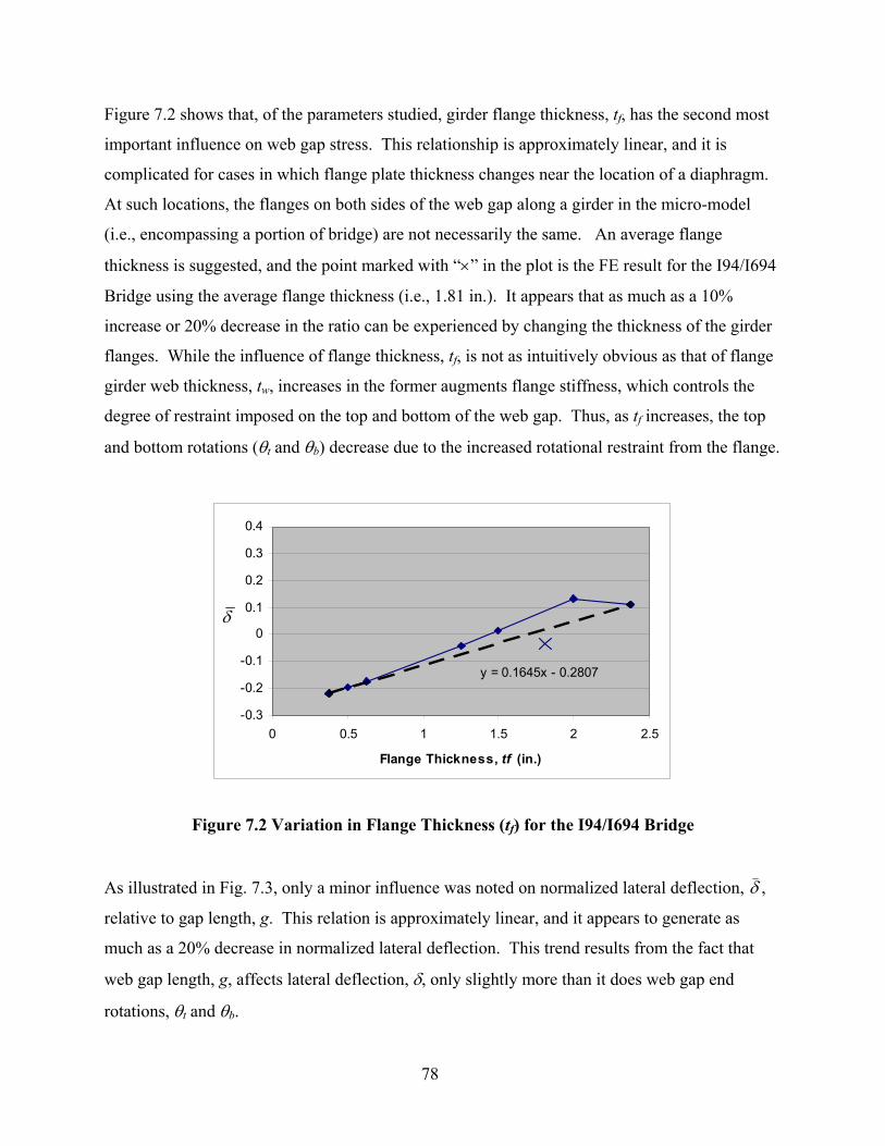
78

Figure 7.2 shows that, of the parameters studied, girder flange thickness, tf, has the second most

important influence on web gap stress. This relationship is approximately linear, and it is

complicated for cases in which flange plate thickness changes near the location of a diaphragm.

At such locations, the flanges on both sides of the web gap along a girder in the micro-model

(i.e., encompassing a portion of bridge) are not necessarily the same. An average flange

thickness is suggested, and the point marked with “×” in the plot is the FE result for the I94/I694

Bridge using the average flange thickness (i.e., 1.81 in.). It appears that as much as a 10%

increase or 20% decrease in the ratio can be experienced by changing the thickness of the girder

flanges. While the influence of flange thickness, tf, is not as intuitively obvious as that of flange

girder web thickness, tw, increases in the former augments flange stiffness, which controls the

degree of restraint imposed on the top and bottom of the web gap. Thus, as tf increases, the top

and bottom rotations (θt and θb) decrease due to the increased rotational restraint from the flange.

Figure 7.2 Variation in Flange Thickness (tf) for the I94/I694 Bridge

As illustrated in Fig. 7.3, only a minor influence was noted on normalized lateral deflection, δ ,

relative to gap length, g. This relation is approximately linear, and it appears to generate as

much as a 20% decrease in normalized lateral deflection. This trend results from the fact that

web gap length, g, affects lateral deflection, δ, only slightly more than it does web gap end

rotations, θt and θb.

y = 0.1645x - 0.2807

-0.3

-0.2

-0.1

0

0.1

0.2

0.3

0.4

0 0.5 1 1.5 2 2.5

Flange Thickness, tf (in.)

δ

79

y = 0.1154x - 0.3659

-0.3

-0.2

-0.1

0

0.1

0.2

0.3

0.4

1.5 2 2.5 3 3.5

Web Gap Length, g (in.)

Figure 7.3 Variation in Web Gap Length (g) for I94/I694 Bridge

-0.3

-0.2

-0.1

0

0.1

0.2

0.3

0.4

0.02 0.04 0.06 0.08 0.1 0.12 0.14

Differential Deflection, ∆ (in.)

Figure 7.4 Variation in Differential Deflection (∆) for I94/I694 Bridge

Differential deflection was observed in Figure 7.4 to have no clear trend with lateral deflection.

Moreover, the mean value for normalized lateral deflection, δ , vanishes for the range of

differential deflections considered. This behavior arises from the fact that girder differential

deflection, ∆ (which is also diaphragm deflection) affects web gap lateral deflection, δ, in the

same proportion as the end rotations (θt and θb).

80

The last parameter studied, deck thickness (td), shows no change in normalized lateral deflection

over the range of thicknesses considered. It appears that the influence of deck stiffness on girder

web gap flexibility is saturated even for the smallest deck thickness considered (i.e., 8 in.), and

that any further increase in td cannot produce a significant change in δ .

-0.3

-0.2

-0.1

0

0.1

0.2

0.3

0.4

7.5 8 8.5 9 9.5 10 10.5

Deck Thickness, t d (in.)

Figure 7.5 Variation in Deck Thickness (td) for I94/I694 Bridge

7.3 Approximating Web Gap Lateral Deflection

For the first three parameters studied in the I94/I694 Bridge, namely tw, tf and g, linear

approximations of the trends shown in Figures 7.1-7.3 can be used to approximate the computed

behavior of the web gaps. These approximations can be quantified using multivariate linear

regression analysis of the FE data. However, given the limited scope of the numerical study, and

even more limited field measurements of web gap lateral displacement, there is insufficient data

for a rigorous statistical analysis of δ. Yet, it is possible to use the results generated in the FE

diaphragm study to define general trends in web gap lateral deflection for the I94/I694 Bridge.

In the present study, it is assumed, purely for the sake of simplification, that the parameters

affecting web gap lateral deflection are independent. Thus, normalized web gap lateral

deflection can be approximated as

81

43f2w1 DgDtDtD +++=δ Equation 7.2

in which the cross-coupling terms (i.e., D5twtf, D6twg, D7tfg and D8twtfg) are assumed to be

negligible. The constants D1-D3 in Equation 7.2 were obtained from the assumed linear

variations in the FE data shown by dashed lines in Figures 7.1-7.3. The coefficient D4 was

obtained as the average of the three values calculated from the linear approximations shown

Figures 7.1-7.3 (i.e., substituting D1-D3 and known parameters (tw, g or tf) into Equation 7.2, then

comparing with the linear equations in Figures 7.1-7.3 respectively to get D4). The resulting

values for D1, D2, D3, D4 in Equation 7.2 for the I94/I694 Bridge are listed in Table 7.2.

Substituting into Equation 7.2 g = 2.5 in., tw = 0.5 in., tf = 1.81 in. (i.e., the “original” parameter

values for the diaphragm studied in I94/I694 Bridge) gives 031.0−=δ , which matches the finite

element computed normalized deflection of 033.0−=δ to within 7%.

Table 7.2 Constants in Equation 7.2 for Variations of I94/I694 Bridge Constants (tw, tf and g are all in inches) Bridge D1 D2 D3 D4

I94/I694 Bridge -1.6586 0.1645 0.1154 0.2121

Several comments are in order. First, it is not certain if the expression assumed in Equation 7.2

is applicable for general use, because there is insufficient data from the FE parameter study for

its verification. For example, there is no data to verify that all cross-coupling terms are

negligible. Also, in some cases a linear approximation is an overly simplistic representation of

computed web gap deflection behavior (e.g., Figure 7.1). Second, there is insufficient field data

to justify formulas for web gap lateral deflection: Only two bridges have been monitored as part

of the ongoing Mn/DOT research program, and the field measurements for δ indicate negligible

lateral deflection of the instrumented web gaps. A broader instrumentation program is needed to

provide a more comprehensive database of field measurements from which to characterize δ.

The exercise summarized above, and the computed constants for Equation 7.2, are intended to

apply only to the I94/I694 Bridge.

82

7.4 FE Diaphragm Study of Plymouth Ave. Bridge

The web gap lateral deflections and end rotations were computed in the FE diaphragm study of

the Plymouth Ave. Bridge. The values of the varied parameters (i.e., girder web thickness, tw,

girder flange thickness, tf, web gap length, g, differential deflection, ∆, and deck thickness, td,

respectively.), the corresponding responses and the normalized web gap deflection, δ , are listed

in Table 7.3, and the values contained in the original model (i.e., the model that best represents

the Plymouth Ave. Bridge) are also noted.

Table 7.3 FE Model Results of Web Gap Deformation for the Plymouth Ave. Bridge Parameter

Changed Value (in.) tθ bθ δ (in.) δ

g 1.7 0.000446 0.00025 -0.00017 -0.106 g 2 0.000438 0.000253 -0.00012 -0.064 g 2.3 0.000442 0.000256 -0.00005 -0.023

Original g 2.5 0.000441 0.000258 0 0 g 2.7 0.00044 0.00026 0.00006 0.023 g 3 0.000439 0.000263 0.00015 0.052 g 3.3 0.000438 0.000265 0.00025 0.078 tw 0.4375 0.000462 0.000265 0.00082 0.331 tw 0.5 0.000448 0.000259 0.00033 0.137

Original tw 0.5625 0.000441 0.000258 0 0 tw 0.625 0.000431 0.000254 -0.00021 -0.089 tw 0.75 0.000416 0.000253 -0.00046 -0.2

Original ∆ 0.03882 0.000441 0.000258 0 0 ∆ 0.02591 0.000327 0.000196 0.00006 0.033 ∆ 0.03394 0.000333 0.000233 0.00006 0.030 ∆ 0.02128 0.000213 0.000145 0.0001 0.080 ∆ 0.01837 0.000184 0.000126 0.000116 0.107 td 8 0.00049 0.000279 -0.000037 -0.014

Original td 9 0.000441 0.000258 0 0 td 10 0.000397 0.000235 0.0000248 0.011 tf 0.375 0.000137 0.000178 0.00021 0.171 tf 0.5 0.000372 0.000318 0.00005 0.020 tf 0.65 0.000357 0.000266 0.00003 0.013

Original tf 1.125 0.000441 0.000258 0 0 tf 2 0.000425 0.000218 0.0002 0.093 tf 2.5 0.000413 0.000202 0.00026 0.127

Figures 7.6-7.10 illustrate the variation in normalized web gap deflection, δ , with the parameters

investigated in Table 7.3 respectively. These plots show trends similar to those observed for the

I94/I694 Bridge, with three parameters exhibiting finite (i.e., non-zero) influence on normalized

83

lateral deflection, namely tw, tf, and g. Of these parameters, tw has the greatest influence and g

has the least influence on δ . Differential deflection, ∆, was observed in Figure 7.9 to have a

mean value close to zero for the range of differential deflections considered, and no change was

observed in normalized lateral deflection with deck thickness, td (Figure 7.10).

y = -1.424x + 0.801

-0.3

-0.2

-0.1

0

0.1

0.2

0.3

0.4

0.3 0.4 0.5 0.6 0.7 0.8Web Thickness, t w (in.)

Figure 7.6 Variation in Web Thickness (tw) for the Plymouth Ave. Bridge

y = 0.0535x - 0.0068

-0.3

-0.2

-0.1

0

0.1

0.2

0.3

0.4

0 0.5 1 1.5 2 2.5 3

Flange Thickness, t f (in.)

Figure 7.7 Variation in Flange Thickness (tf) for the Plymouth Ave. Bridge

84

y = 0.115x - 0.3015

-0.3

-0.2

-0.1

0

0.1

1.5 2 2.5 3 3.5

Web Gap Length, g (in.)

Figure 7.8 Variation in Web Gap Length (g) for the Plymouth Ave. Bridge

-0.1

0

0.1

0.2

0.3

0.01 0.015 0.02 0.025 0.03 0.035 0.04 0.045

Differential Deflection, ∆ (in.)

Figure 7.9 Variation in Differential Deflection (∆) for Plymouth Ave. Bridge

The same approximate multivariate linear regression analysis used for the I94/I694 Bridge was

applied to the computed normalized deflection data from the FE diaphragm study of the

Plymouth Ave. Bridge. For each of the three diaphragm parameters of importance, one was

varied while the others were held constant. Equation 7.2 is found to be a reasonable preliminary

approximation for the normalized lateral deflection, δ of the Plymouth Ave. Bridge.

85

-0.3

-0.2

-0.1

0

0.1

0.2

0.3

0.4

7.5 8 8.5 9 9.5 10 10.5

Deck Thickness, t d (in.)

Figure 7.10 Variation in Deck Thickness (td) for Plymouth Ave. Bridge

Using the same procedure that was used for the I94/I694 Bridge, coefficients D1, D2, D3, D4 were

computed for the diaphragm parameter study of Plymouth Ave. Bridge, and the values for these

constants are shown in Table 7.4.

Table 7.4 Constants in Equation 7.2 for Variations of Plymouth Ave. Bridge Constants (tw, tf and g are all in inches) Bridge Studied D1 D2 D3 D4

Plymouth Ave. Bridge -1.424 0.0535 0.115 0.4664

Substituting tw = 0.5625 in., tf = 1.125 in., g = 2.5 in. (the original values of the diaphragm

studied in Plymouth Ave. Bridge) into Equation 7.2 gives 013.0−=δ , which is close to the value

of 0 computed using the FE analysis.

7.5 Discussion

It is interesting to note that the values for constants D1 and D3 are similar for both bridges studied,

but those for constants D2 and D4 are considerably different. This observation raises questions

regarding the values of these parameters, as well as the other constants in Equation 7.2, if

diaphragms in other bridges were analyzed. As a simple exercise to test this notion, mean values

86

for constants D1 – D4 for both bridges in the present study are found to be -1.54, 0.109, 0.115 and

0.339, respectively. Using these mean values, normalized lateral displacements equal to 0.054

and -0.117, respectively, were computed for the I94/I694 and Plymouth Ave. Bridges using

Equation 7.2. While these approximations for δ are not as close to the FE computed values as

the ones computed earlier with the bridge specific constants (D1 – D4), they show some promise

that a formula like that given by Equation 7.2 can be used to estimate web gap lateral deflections

with an acceptable degree of accuracy.

If normalized web gap lateral displacement,δ , can be predicted accurately, its contribution can

be included in the web gap stress formula given by Equation 2.5 as follows

∆

⋅+⋅=

Sgt

EC wwg )31( δσ Equation 7.3

Until a more accurate procedure is developed, Equation 7.2 is used for estimating δ .

With the values of constants D1 – D4 in Tables 7.2 and 7.4 for each bridge in the present study,

Equation 7.2 was used to predict the normalized lateral deflection, δ , and it was included in

Equation 7.3 for a refined prediction of web gap stress. The results for stress prediction with δ

(Equation 7.3) and without δ (Equation 5.2) in the diaphragm study of I94/I694 Bridge and

Plymouth Ave. Bridge were listed in Tables 7.5 and 7.6 respectively. The values contained in

the “original” model (i.e., that best represents the I94/I694 Bridge/Plymouth Ave. Bridge) are

also noted in the first column of each table.

The results show that Equation 7.3 in conjunction with the normalized lateral deflection (δ )

predicted from Equation 7.2 gave closer results to finite element stresses than Equation 5.2,

which means that the inclusion of lateral deflection increased the estimation accuracy of peak

web gap stress. The over prediction of stresses from Equation 5.2 for short web gap length (g),

thick web thickness (tw) and thin flange thickness (tf) was effectively mitigated when lateral

deflection (δ) was included in the stress prediction. Though the results with δ in Tables 7.5 and

7.6 are not as good as those in Tables 5.3 and 6.6 (the latter calculated stresses with the lateral

87

deflection δ from finite element analyses directly), it is essential to identify the importance of

lateral deflection on the accuracy of stress prediction and give a preliminary estimation of the

influence of δ through this study.

Table 7.5 Comparison of Stress Prediction without and with Proposed Lateral Deflection for I94/I694 Bridge

Prediction (C=2.25) FE Model

Results w/o δ (Eq. 5.2)

with δ (Eq. 7.3) Parameter

Changed Value (in.)

wgσ (ksi) 1+3δ

wgσ (ksi) wgσ (ksi) g 1.7 9.55 0.63 22.26 14.02 g 2 8.95 0.73 18.92 13.81 g 2.3 9.9 0.84 16.45 13.82

Original g 2.5 15.94 0.91 15.14 13.78 g 2.7 14.68 0.98 14.01 13.73 g 3 15.4 1.08 12.61 13.62 g 3.3 16.75 1.18 11.47 13.53 tw 0.375 37.98 1.53 12.08 18.48 tw 0.4375 24.26 1.22 13.64 16.64

Original tw 0.5 15.94 0.91 15.14 13.78 tw 0.5625 10.65 0.60 16.57 9.94 tw 0.625 7.22 0.28 17.96 5.03 tw 0.75 3.39 -0.34 20.57 -6.99

Original ∆ 0.12874 15.94 0.91 15.14 13.78 ∆ 0.11179 17.32 0.91 13.14 11.96 ∆ 0.06517 7.33 0.91 7.66 6.97 ∆ 0.04658 5.36 0.91 5.48 4.99 ∆ 0.03012 6.87 0.91 3.54 3.22 td 8 15.95 0.91 15.19 13.82

Original td 9 15.94 0.91 15.14 13.78 td 10 13.56 0.91 12.38 11.27 tf 0.375 7.72 0.20 22.78 4.56 tf 0.5 9.51 0.26 21.53 5.60 tf 0.625 11.16 0.32 20.48 6.55 tf 1.25 15.47 0.63 15.28 9.63 tf 1.5 19.04 0.75 16.00 12.00 tf 2 20.22 1.00 13.39 13.39 tf 2.375 23.84 1.19 13.73 16.34

Original tf 1.81 15.94 0.91 15.14 13.78

88

Table 7.6 Comparison of Stress Prediction without and with Proposed Lateral Deflection for Plymouth Ave. Bridge

Prediction (C=2.75) FE Model w/oδ

(Eq. 5.2) with δ

(Eq. 7.3) Parameter Changed Value (in.)

wgσ (ksi)

1+3δ

wgσ (ksi) wgσ (ksi) G 1.7 6.39 0.76 9.15 6.95 G 2 7.44 0.87 7.77 6.76 G 2.3 8.4 0.97 6.76 6.56

Original G 2.5 8.23 1.04 6.22 6.47 G 2.7 9.75 1.11 5.76 6.39 G 3 10.73 1.21 5.18 6.27 G 3.3 11.44 1.32 4.71 6.22 tw 0.4375 17.43 1.57 4.95 7.77 tw 0.5 11.74 1.31 5.59 7.32

Original tw 0.5625 8.23 1.04 6.22 6.47 tw 0.625 5.76 0.77 6.84 5.27 tw 0.75 3.04 0.24 8.06 1.93

Original ∆ 0.03882 8.23 1.04 6.22 6.47 ∆ 0.02591 7.29 1.04 5.44 5.66 ∆ 0.03394 7.43 1.04 4.15 4.32 ∆ 0.02128 5.34 1.04 3.41 3.55 ∆ 0.01837 4.9 1.04 2.94 3.06 td 8 8.59 1.04 6.82 7.09

Original td 9 8.23 1.04 6.22 6.47 td 10 7.66 1.04 5.69 5.92 tf 0.375 4.81 0.92 3.86 3.55 tf 0.5 7.29 0.94 7.20 6.77 tf 0.65 6.87 0.96 6.13 5.88

Original tf 1.125 8.23 1.04 6.22 6.47 tf 2 10.01 1.18 5.59 6.60 tf 2.5 10.21 1.26 5.37 6.77

It was noted earlier, however, that there is some uncertainty concerning the use of Equation 7.2

for approximating δ . Even if Equation 7.2 were applicable for a wide selection of bridges, the

choice of numerical values for constants D1 – D4 is unknown for such a selection. It is also

known from the bridge parameter studies of the I94/I694 and Plymouth Ave. Bridges that girder

spacing, S, angle of skew, sβ , span length, L, and the location of the diaphragms relative to the

nearest pier can have an impact on the value of web gap lateral deflection, δ, and web gap end

89

rotations, θt and θb. Whether or not these bridge parameters also affect δ remains to be

determined.

The approximation of the normalized lateral deflection, δ , may be more complicated than that

identified in this chapter. A program combining field instrumentation and finite element analysis

of a wider selection of bridges from the Mn/DOT inventory is required to establish a better

understanding of the influence of lateral deflection on web gap stress. However, in lieu of

additional research, Equation 7.3 can be used in conjunction with the values for constants D1 –

D4 to obtain a gross estimate of δ for those bridges in which web gap lateral deflections are

known to be important (i.e., 3.0±≥δ ).

90

Chapter 8 - Summary and Conclusions

The research documented in this report advances the understanding of the distortion-induced

fatigue problem and enhances the ability to rapidly assess peak web gap stresses in multi-girder

steel bridges. A comprehensive literature review of documented past research on field and

laboratory measurements helps to identify the mechanisms for this phenomenon, and effective

retrofitting solutions have been presented in these documents. The literature review provides a

basis for future investigations.

Previous research sponsored by the Mn/DOT led to the development of a simple formula

(Equation 2.2) equation for the prediction peak web gap stress [1]. This research was based upon

field monitoring and finite element modeling of the instrumented portion of a skew supported

bridge, and the stress equation requires knowledge of bridge geometry, as well as the expected

maximum differential deflection at a diaphragm location. In another Mn/DOT project, a formula

for the prediction of maximum differential deflection (Equation 2.3) was developed from the

results of an extensive parameter study using finite element models of bridges with bent-plate

diaphragms [2]. A different stress prediction formula (Equation 2.6) was proposed in a third

Mn/DOT research, and this equation was derived from a parameter study performed using the

finite element model of an instrumented portion of a skew bridge with cross-brace diaphragms

[3]. In addition, this research effort suggested a correction factor for the reduction of maximum

differential deflection of cross-brace diaphragms compared with that for bent-plate diaphragms

(Equation 2.7) on the basis of finite element model analyses of multi-girder steel bridges [3]. At

the conclusion of these three previous projects, further research was still required to calibrate the

finite element models and evaluate the applicability of previous prediction methods, including

the web gap stress and the differential deflection formulas.

Dual-level analyses incorporating both finite element micro-models (i.e., encompassing a portion

of bridge surrounding the studied diaphragm) and macro-models (i.e., encompassing the entire

bridge) were performed in the present Mn/DOT research project to account for the uncertainties

of boundary conditions introduced by the substructure models. The models for both bridges that

91

were previously instrumented were calibrated, and the diaphragm responses to bridge loads were

evaluated through dual-level finite element analyses. As a result, the general stress formula

based upon linear beam theory (Equation 2.5) was found to be appropriate for future study on

stress calculation.

With the calibrated finite element models and stress formula available, parameter studies were

performed on prototypical variations of both I94/I694 and Plymouth Ave. Bridges to define the

sensitivity of diaphragm stress responses to typical bridge parameters. Parameter studies were

divided into two categories: diaphragm parameter study for the effects of typical diaphragm

parameters (i.e., web gap length, web thickness, girder flange thickness, differential deflection)

and bridge parameter study for the effects of typical bridge parameters (i.e., span length, angle of

skew, girder spacing). Through diaphragm parameter study, it was found that the terms of web

gap rotations in the stress formula normalized by the ratio of differential deflection to girder

spacing were fairly consistent with varying parameters. A constant coefficient C was defined to

represent this ratio. The bridge parameter study showed that the coefficient can be approximated

as linear functions of span length for diaphragms near the pier (Equation 5.3 (b)) and away from

the pier (Equation 5.3 (a)), and that skew angle and girder spacing have negligible influence on

the prediction of web gap stress. Thus, the previously proposed stress formulas (Equations 2.2

and 2.6) were calibrated with current findings.

Girder differential deflection was determined not to be well predicted by Equation 2.3 proposed

by Berglund [2] in conjunction with the correction factor (Equation 2.7) suggested for cross-

brace diaphragms by Beukema [3] for the following cases: 1) bridges under truck loadings with

different configurations from standard HS-20/HS-15 trucks; 2) cross-brace diaphragms with

girder spacing other than 10.5 ft; 3) bridges with additional sidewalk railing systems. Finite

element models for entire bridges under these three cases were analyzed and the maximum

differential deflections were computed. Thus, modification factors RL, Rx and Rd (Equations 5.4,

2.7 and 6.1, respectively) for use with Berglund’s deflection formula were proposed for the cases

mentioned above. The prediction of maximum differential deflection combined with the

constant coefficient in the stress formula gives satisfactory estimates for the peak web gap

stresses of both bent-plate and cross-brace diaphragm bridges, if there is evidence that the lateral

92

deflection of web gap can be negligible. The formulas for bridges with bent-plate diaphragms

are given by: Equations 2.3, 5.2 and 5.3, and for bridges with cross-brace diaphragms the

required formulas are: Equations 2.3, 2.7, 5.2 and 5.3. In addition, 1) if the response to 50-kip

sand trucks is desired, instead of that for an HS-20 truck, the correction factor RL (Equation 5.4)

is needed for differential deflection; 2) if an added sidewalk is used in the bridge, correction

factor Rd given by Equation 6.1 is needed for differential deflection.

This study included evaluation of web gap lateral deflection in the diaphragm parameter studies

of the I94/I694 and Plymouth Ave. Bridges. The influence of lateral deflection, relative to both

top and bottom rotations of the web gap, was studied under varying diaphragm parameters (i.e.,

web thickness, web gap length, girder flange thickness, girder differential deflection and deck

thickness). It was noted that the lateral deflection did not change much with the variations of

girder differential deflection and deck thickness. Thus, the ratio of the term representing lateral

deflection to the terms including top and bottom rotations in the stress formula was approximated

as a multivariate linear equation with three parameters: web thickness, web gap length and girder

flange thickness. This preliminary evaluation was conducted to gain a qualitative understanding

of the sensitivity of lateral deflection to the various diaphragm parameters of importance in the

web gap distortional fatigue problem. Therefore, simplifying assumptions, the justification of

which is not known due to the lack of field data on web gap lateral deflection, were made to

facilitate this qualitative analysis. Nonetheless, as a result of this study, it was determined that

the constant coefficient in the proposed stress prediction formula (Equation 5.2) can be further

calibrated with the consideration of lateral deflection (Equation 7.3). The influence of lateral

deflection on web gap stress prediction is a much more complicated problem than identified

above since it may also depend on the bridge parameters (e.g., span length, girder spacing, angle

of skew, and location of the diaphragm) which were not studied relative to lateral deflection.

With the completion of the present study, a thorough finite element study for various bridges in

the Mn/DOT bridge inventory has been documented, and proposed procedures for evaluating

girder differential deflections and web gap stresses have been calibrated to increase prediction

accuracy. These prediction tools should prove to be effective for the rapid assessment of bridges

susceptible to distortional fatigue problems. The only shortcoming of the present study is that

93

the technique for incorporating lateral deflection in the web gap stress prediction formula has not

been fully validated. Future research is required to verify and/or modify the proposed procedure

for web gap lateral deflection with field measurements and detailed finite element analyses (i.e.,

using the dual-level analysis procedure developed as part of this study).

94

References

1. Jajich, D., Schultz, A.E., Bergson, P.M., and Galambos, T.V. “Distortion-Induced Fatigue in Multi-Girder Steel Bridges.” Minnesota Department of Transportation, Final Report, May 2000.

2. Berglund, E., Schultz, A.E. “Girder Differential Deflection and Assessing Distortional

Fatigue in Skewed Steel Bridges.” Minnesota Department of Transportation, Final Report, Dec. 2001.

3. Severtson, B., Beukema, F., Schultz, A.E. “Rapid Assessment of Distortional Stresses in

Multi-Girder Steel Bridges.” Minnesota Department of Transportation, Final Report, July 2004.

4. Keating, Peter. “Focusing on Fatigue.” Civil Engineering, Nov. 1994, 54-57. 5. Fisher, J.W. Fatigue and Fracture in Steel Bridges: Case Studies. John Wiley and Sons, New

York, 1984. 6. Fisher, John W., Yen, Ben, and Wagner, David. “Review of Field Measurements for

Distortion Induced Fatigue Cracking in Steel Bridges.” Transportation Research Record, n1118, 1987, 49—55.

7. DeWolf, John T., Lindsay, Tod, and Culmo, Michael. “Fatigue Evaluation in Steel Bridges

Using Field Monitoring Equipment.” Building to Last Proceedings of Structures Congress XV, ASCE, Portland, Oregon, April 13th-16th, 1997.

8. Cousins, T. E., et al. “Field Evaluation of Fatigue Cracking in Diaphragm-Girder

Connections.” Journal of Performance of Constructed Facilities, 12(1), 1998, 25—32. 9. Fisher, John W., Jin, Jian, Wagner, David, and Yen, Ben. “Distortion Induced Fatigue

Cracking in Steel Bridges.” NCHRP Report 336, Transportation Research Board, National Research Council, Washington D.C., Dec. 1990.

10. Fisher, John W. “Fatigue Cracking in Bridges from Out-of-Plane Distortion.” Canadian

Journal of Civil Engineering, 5(4), 1978, 542—556. 11. Fisher, John W., Hausammann, Hans, Sullivan, Michael D., and Pense, Allan W. “Detection

and Repair of Fatigue Damage in Welded Highway Bridges.” NCHRP Report 206, Transportation Research Board, National Research Council, Washington D.C., June 1979.

12. Stallings, J.M. and Cousins, T.E. “Laboratory Tests of Bolted Diaphragm-Girder

Connections.” Journal of Bridge Engineering, Vol.3, No.2, May 1998. 13. Keating, Peter and Fisher, John W. “Fatigue Behavior of Variable Loaded Bridge Details

Near the Fatigue Limit.” Transportation Research Record n1118, 1987, 56—64.

95

14. W.M.Kim Roddis, Yuan Zhao. ‘Out-of-Plane Fatigue Cracking in Welded Steel Bridges’,

Welding Innovation Vol. XVIII, No.2, 2001. 15. Yuan Zhao, W.M.Kim Roddis. ‘Fatigue Behavior and Retrofit Investigation of Distortion-

Induced Web Gap Cracking’, 84th TRB Annual Meeting, Jan. 2005. 16. Standard Specifications for Highway Bridges, AASHTO, 16th Edition, Washington, D.C.,

1996. 17. Moses, F., Schilling, C.G., and Raju, K.S. “Fatigue Evaluation Procedures for Steel Bridges.”

NCHRP Report 299, Transportation Research Board, National Research Council, Washington D.C., Nov. 1987.

18. Wipf, T.J., et. al. “Retrofit Methods for Distortion Cracking Problems in Plate Girder

Bridges.” Iowa Department of Transportation, Final Report, Jan. 2003. 19. Stallings, J.M., Cousins, T.E., and Stafford, T.E. “Effects of Removing Diaphragms from a

Steel Girder Bridge.” Transportation Research Record, n1541, Nov. 1996, 183—188. 20. Stallings, J.M., Cousins, T.E., and Stafford, T.E. “Removal of Diaphragms from three-Span

Steel Girder Bridge.” Journal of Bridge Engineering, Vol.4, No.1, 1999. 21. LRFD Bridge Design Manual, Minnesota Department of Transportation, April 2004. 22. Computers and Structures, Inc. SAP2000 NonLinear Version 7.44 Structural Analysis

Program. Berkeley, CA, 2001.

APPENDIX A

ASSESSMENT OF PEAK WEB GAP STRESS IN PLYMOUTH AVE. BRIDGE

A-1

1. Evaluating Girder Differential Deflection

Given the span length of 156.69 ft, girder spacing of 9.33 ft (112 in.), and skew angle of

45.5°, the predicted maximum differential deflection in the Plymouth Ave. Bridge using

Berglund’s formula [2] for AASHTO HS-20 truck (Equation 2.3) is ∆HS-20 = 0.0856 in.

To compare with the data collected under 50-kip sand truck loading, further correction is

required. In Chapter 5, an exponential formula Equation 5.4 was given for the ratio of

maximum differential deflection under the 50-kip sand truck loading and the HS-20 truck

loading, substituting the values of L = 156.69 ft gives:

749.0)69.156(9321.3/ 3282.020HSkip50 =⋅=∆∆= −

−−LR

The girder spacing of 9.33 ft is close to 9.25 ft, so that using the span length and the

constants from Table 6.2 in Equation 2.7 yields a correction factor for cross-brace

diaphragms:

796.0)69.156(10232.3)69.156(10038.11/ 425 =⋅+⋅−=∆∆= −−bpcbxR

Finally, because the Plymouth Ave. Bridge has an added sidewalk that reduces the

maximum differential deflection compared with J-rail, the modification factor Rd can be

approximated using Equation 6.1, which is:

942.07378.0)69.156(0013.0/ =+⋅=∆∆= JSdR

Thus the corrected prediction value of maximum differential deflection for the Plymouth

Ave. Bridge becomes:

.in048.00856.0942.0796.0749.020HS =⋅⋅⋅=∆⋅⋅⋅=∆ −dxL RRR

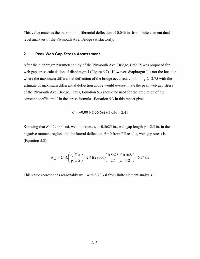
A-2

This value matches the maximum differential deflection of 0.046 in. from finite element dual-

level analyses of the Plymouth Ave. Bridge satisfactorily.

2. Peak Web Gap Stress Assessment

After the diaphragm parameter study of the Plymouth Ave. Bridge, C=2.75 was proposed for

web gap stress calculation of diaphragm J (Figure 6.7). However, diaphragm J is not the location

where the maximum differential deflection of the bridge occurred, combining C=2.75 with the

estimate of maximum differential deflection above would overestimate the peak web gap stress

of the Plymouth Ave. Bridge. Thus, Equation 5.3 should be used for the prediction of the

constant coefficient C in the stress formula. Equation 5.3 in this report gives:

41.2036.3)69.156(004.0 =+⋅−=C

Knowing that E = 29,000 ksi, web thickness tw = 0.5625 in., web gap length g = 2.5 in. in the

negative moment region, and the lateral deflection δ = 0 from FE results, web gap stress is

(Equation 5.2):

ksi74.6112048.0

5.25625.0)29000(41.2 =

=

∆

⋅=

SgtEC w

wgσ

This value corresponds reasonably well with 8.23 ksi from finite element analysis.