ANALYSIS OF CONVECTIVELY COUPLED KELVIN WAVES IN THE INDIAN

OCEAN MJO

Paul E. Roundy

University At Albany

State University of New York

Submitted to

The Journal of the Atmospheric Sciences

November 2006

Revisions Submitted May, July, and August 2007

Corresponding Author Address

Department of Earth and Atmospheric Sciences

DEAS-ES351,

Albany, NY 12222

roundy@atmos.albany.edu

0

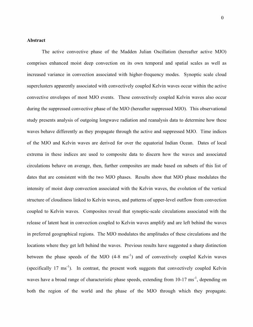
Abstract

The active convective phase of the Madden Julian Oscillation (hereafter active MJO)

comprises enhanced moist deep convection on its own temporal and spatial scales as well as

increased variance in convection associated with higher-frequency modes. Synoptic scale cloud

superclusters apparently associated with convectively coupled Kelvin waves occur within the active

convective envelopes of most MJO events. These convectively coupled Kelvin waves also occur

during the suppressed convective phase of the MJO (hereafter suppressed MJO). This observational

study presents analysis of outgoing longwave radiation and reanalysis data to determine how these

waves behave differently as they propagate through the active and suppressed MJO. Time indices

of the MJO and Kelvin waves are derived for over the equatorial Indian Ocean. Dates of local

extrema in these indices are used to composite data to discern how the waves and associated

circulations behave on average, then, further composites are made based on subsets of this list of

dates that are consistent with the two MJO phases. Results show that MJO phase modulates the

intensity of moist deep convection associated with the Kelvin waves, the evolution of the vertical

structure of cloudiness linked to Kelvin waves, and patterns of upper-level outflow from convection

coupled to Kelvin waves. Composites reveal that synoptic-scale circulations associated with the

release of latent heat in convection coupled to Kelvin waves amplify and are left behind the waves

in preferred geographical regions. The MJO modulates the amplitudes of these circulations and the

locations where they get left behind the waves. Previous results have suggested a sharp distinction

between the phase speeds of the MJO (4-8 ms-1) and of convectively coupled Kelvin waves

(specifically 17 ms-1). In contrast, the present work suggests that convectively coupled Kelvin

waves have a broad range of characteristic phase speeds, extending from 10-17 ms-1, depending on

both the region of the world and the phase of the MJO through which they propagate.

1

1. Introduction

The Madden-Julian Oscillation (MJO, Madden and Julian 1994) is the dominant mode of

intraseasonal variability of the tropical atmosphere. Efforts to explain the leading dynamics of the

oscillation have not led to a consensus. Many marginally successful models for the MJO are based

on moist Kelvin wave dynamics (e.g., Chang and Lim 1988; Cho et al. 1994). However, recent

studies suggest that a leading mode of convectively coupled atmospheric Kelvin waves behaves

differently from the MJO in many respects. These Kelvin waves tend to be smaller-scale features

than the MJO and they tend to propagate at more than twice the phase speed of the MJO (Matsuno

1966; Dunkerton and Crum 1995; Wheeler and Kiladis 1999; Straub and Kiladis 2002; Roundy and

Frank 2004a). Further, although the spectral peak of the MJO intersects with the theoretical Kelvin

wave dispersion line at zonal wavenumber 1, spectral power associated with the MJO is spread

broadly across wavenumbers 0 to 10. Power associated with convectively coupled Kelvin waves is

spread more broadly across the spectrum in frequency, but at each frequency where it occurs, it is

largely concentrated within a narrow range of wavenumbers (Wheeler and Kiladis 1999; Roundy

and Frank 2004a).

The active MJO has long been described as an eastward moving envelope of enhanced

convection and enhanced variability in convection organized on smaller scales. Modes of organized

convection interact across a broad range of spatial and temporal scales to generate a hierarchical

sub-structure of organized cloudiness that is observed during nearly every MJO active convective

event (e.g., Majda et al. 2004; Mapes et al. 2006; and references therein). This sub-structure

consists of eastward-and westward-moving superclusters, which in turn comprise smaller westward-

moving cloud clusters. Synoptic-scale eastward-moving superclusters (hereafter, labeled

“superclusters” for simplicity) have been linked to convectively coupled Kelvin waves (Nakazawa

1988; Takayabu and Murakami (1991); Dunkerton and Crum 1995; Wheeler and Kiladis 1999;

2

Straub and Kiladis 2002), whereas westward-moving elements relate to equatorial Rossby waves

(Kiladis and Wheeler 1995; Wheeler et al. 2000; Roundy and Frank 2004b), mixed Rossby gravity

waves (e.g., Hendon and Liebmann 1991; Dickinson and Molinari 2002), easterly waves or tropical

depression type disturbances, westward inertio gravity waves, and tropical cyclones (e.g., Maloney

and Hartman 2001; Frank and Roundy 2006). The MJO also triggers Kelvin waves in the ocean

(e.g., Hendon et al. 1998). These oceanic waves modulate the development of some MJO events

because atmospheric convection responds to sea surface temperature changes induced by the waves

(Roundy and Kiladis 2006). Although the extent of the relevance of each of these smaller-scale

modes to the behavior of the MJO requires further study, each of these eastward and westward-

moving modes apparently interact with and modulate each other and might modulate the behavior

of the MJO itself. The convectively coupled atmospheric Kelvin wave (hereafter referred to as

“Kelvin wave” for simplicity) described by Wheeler and Kiladis (1999), Straub and Kiladis (2002,

2003a, 2003b), Roundy and Frank (2004a), and others may be a fundamental part of the anatomy of

many MJO events. Kelvin waves are observed during each of the phases of the MJO, but those that

occur during the active convective phase (hereafter “active MJO”) have higher amplitudes and are

observed more frequently (e.g., Dunkerton and Crum 1995). Since the MJO modulates the

background state through which these waves propagate, wave structure and propagation

characteristics may also change with the phase of the MJO. This type of modulation is considered

nonlinear if the combination of the MJO and the Kelvin waves differs from the simple linear sum of

the two processes.

The phase speed generally associated with Kelvin waves is near 17 ms-1 (Wheeler and Kiladis

1999; Straub and Kiladis 2002) whereas the phase speed Dunkerton and Crum (1995) reported for

these waves over the Indian Ocean was 10-13 ms-1 (see also Takayabu and Murakami 1991),

suggesting that the waves might be characterized by different phase speeds in different regions of

3

the world. Although not discussed in the works in which it was shown, previous analysis suggests

that anomalies of convection associated with convectively coupled Kelvin waves do not tend to

move at the same phase speeds when characterized by different spatial scales. The wavenumber-

frequency spectra shown in Fig. 3b of Wheeler and Kiladis (1999) and Figs. 2 b and c and 4 of

Roundy and Frank (2004a) show the Kelvin wave peak following the h=50m dispersion line near

wavenumber 2 and the 25m dispersion line near wavenumber 7, suggesting the tendency for

smaller-scale Kelvin waves to propagate more slowly than larger-scale waves (see also Fig. 1,

shown below). Many different types of waves amplify and reduce in spatial scale as they propagate

through the active MJO (Maloney and Hartmann 2001; Dickinson and Molinari 2002; Liebmann et

al. 1994; and many others). These conclusions together suggest that these waves might propagate

more slowly on average during the active MJO than during the suppressed MJO. Although these

results suggest possible wave dispersion associated with convectively coupled Kelvin waves, the

different phase speeds are more likely linked to variations in convective coupling or propagation

through different background environments.

As an envelope of active MJO convection approaches a given region from the west, local

convection evolves in time following a particular general pattern. Shallow trade cumuli increase in

prevalence, developing into cumulus congestus (which preconditions the atmosphere for moist deep

convection by moistening the mid levels), then deep convection abruptly begins, trailing into high

altitude-based nimbostratus before clearing (e.g., Johnson et al. 1999; Khouider and Majda 2007).

In general, smaller-scale convective elements evolve similarly (e.g., Haertel and Kiladis 2004;

Kiladis et al. 2005; and others). This pattern appears to be loosely independent of spatial and

temporal scale, although the mechanisms responsible for the behavior observed on the different

scales are probably not identical. Mapes et al. (2006) suggest a “stretched building block”

hypothesis to describe how this pattern can be maintained on the spatial and temporal scales of the

4

MJO. This hypothesis suggests that smaller scale convective elements within a region of the MJO

superstructure spend more time than average in the phase of cloudiness that dominates the local

state of the MJO, thereby reinforcing the state of evolution of convection within the MJO. If this

hypothesis accurately describes the evolution of cloudiness in the MJO, then cloudiness associated

with Kelvin waves would also evolve differently during different phases of the MJO. The purpose

of this paper is to analyze atmospheric Kelvin waves in the Indian Ocean basin in the context of

their relationship to the local MJO, to determine how their structures evolve during the different

phases of the MJO.

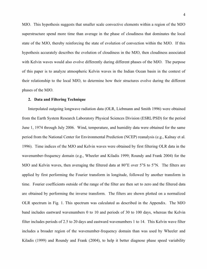
2. Data and Filtering Technique

Interpolated outgoing longwave radiation data (OLR, Liebmann and Smith 1996) were obtained

from the Earth System Research Laboratory Physical Sciences Division (ESRL/PSD) for the period

June 1, 1974 through July 2006. Wind, temperature, and humidity data were obtained for the same

period from the National Center for Environmental Prediction (NCEP) reanalysis (e.g., Kalnay et al.

1996). Time indices of the MJO and Kelvin waves were obtained by first filtering OLR data in the

wavenumber-frequency domain (e.g., Wheeler and Kiladis 1999; Roundy and Frank 2004) for the

MJO and Kelvin waves, then averaging the filtered data at 80°E over 5°S to 5°N. The filters are

applied by first performing the Fourier transform in longitude, followed by another transform in

time. Fourier coefficients outside of the range of the filter are then set to zero and the filtered data

are obtained by performing the inverse transform. The filters are shown plotted on a normalized

OLR spectrum in Fig. 1. This spectrum was calculated as described in the Appendix. The MJO

band includes eastward wavenumbers 0 to 10 and periods of 30 to 100 days, whereas the Kelvin

filter includes periods of 2.5 to 20 days and eastward wavenumbers 1 to 14. This Kelvin wave filter

includes a broader region of the wavenumber-frequency domain than was used by Wheeler and

Kiladis (1999) and Roundy and Frank (2004), to help it better diagnose phase speed variability

5

observed associated with individual wave anomalies seen in unfiltered OLR. Tests show that this

filter is broad enough to avoid significant spectral ringing effects in spite of the sharp cut-offs of the

filter in wavenumber-frequency space (not shown). The expanded filter also allows the filtered data

to diagnose patterns relevant to the waves as manifest in other variables. Wheeler and Kiladis

(1999) suggest that the spectra associated with Kelvin waves and the MJO vary between OLR and

dynamical variables such as temperature and wind. The broad filters applied here should

accommodate most signals relevant to Kelvin waves and the MJO in all of the datasets analyzed

here. If narrower filter bands were applied instead, each dataset might require a different filter to

isolate the relevant signals. Another important potential concern is that signal from the MJO might

also be present in the Kelvin band. However, the Kelvin and MJO filters are well separated within

the wavenumber-frequency domain—the 20-30 day band is excluded from both filters. Although it

is possible that some signals in the Kelvin band are harmonic with the MJO (especially in the 15-20

day range), Wheeler et al. (2000) showed that Kelvin waves produce the dominant coherent signal

in eastward propagation in the 3-20 day band. Eastward inertio gravity waves also occur in the

band, but these produce less OLR variance than Kelvin waves, and since they are antisymmetric

across the equator, their signals are largely removed from the Kelvin time index by the cross-

equatorial averaging used to derive the index.

Nonlinear interactions between waves such as those suggested here would invalidate the strict

superposition principle for convectively coupled waves assumed in many studies (e.g., Wheeler and

Kiladis 1999; Roundy and Frank 2004a). However, the filtering method remains effective in

diagnosing the portions of both the waves themselves and the contributions of nonlinear modulation

effects that occur in the same filter band. Nonlinear interactions might also produce anomalies that

occur outside of the wavenumber-frequency bands of either of the interacting modes. Both filtered

6

and unfiltered data are utilized here to generate composites, to discern the patterns associated with

nonlinear behavior that occur both in and out of the Kelvin band.

3. Compositing Technique

Composites were made by averaging unfiltered or Kelvin filtered data over sets of dates (and

time lags from those dates) obtained from analysis of the MJO and Kelvin wave time indices. Lists

of dates of local maxima and local minima in the MJO index were generated, and another list of

dates was made including all local minima in the Kelvin wave index. The lists of minima (maxima)

were generated by finding all dates on which the index was less (greater) than the index values on

both the preceding and the following days. Dates were then eliminated from the lists if the

corresponding values of the time indices were not more than 1 standard deviation (SD) above or

below zero (to exclude low-amplitude noise). The resulting primary list of Kelvin wave OLR

minima included 891 members. Two subsets of the Kelvin wave date list were made based on the

phase of the MJO in which they occurred. The first subset included only those Kelvin wave events

that occurred within 5 days before and after MJO OLR minima. This subset included 158 members.

The second subset included only those Kelvin waves that occurred within 5 days before or after

MJO OLR maxima. This subset included 130 events. Composite Kelvin waves were generated

based on averaging filtered and unfiltered data over these three sets of dates. Unfiltered data

applied here have the MJO frequency band (30-100 day periods) subtracted since some composites

are made with reference to the MJO but the MJO is not the focus of the analysis.

These two subsets are both smaller than the set of Kelvin wave events potentially modulated by

either phase of the MJO. Although many other Kelvin wave events could be included in the

subsets, this method ensures that composites calculated for these events retain a well-defined

pattern of MJO phase (see below). Note that the subset of dates during the active MJO is longer

than the set for the suppressed MJO. Dunkerton and Crum (1995) suggest that these waves occur

7

more frequently during the active MJO than other times, so it is useful to examine the distribution

of MJO band OLR anomalies on the dates of these Kelvin wave events. Figure 2 is a histogram of

the values of the MJO index on the dates of the Kelvin wave index minima. This result suggests

that although high-amplitude Kelvin waves occur during all stages of the MJO, approximately 24%

more occur when the local MJO OLR anomaly is negative than when it is positive.

The probability that individual composite anomalies are significantly different from zero was

assessed by applying 1000 bootstrap experiments (as in Roundy and Frank 2004b). These

experiments were performed by randomly selecting new samples of events from the original

sample, and generating a new composite for each new sample. Any individual event was allowed to

be drawn any number of times when selecting a new sample. This process results in a distribution

of composite values at each grid point and time lag. The probability that each composite anomaly is

significantly different from zero is determined by locating the zero anomaly line within the

distribution, assuming the null hypothesis that the actual mean value is zero. Further similar tests

were applied to determine the significance of the differences between composites generated for the

convectively active and suppressed phases of the MJO, by comparing the two relevant bootstrap

distributions and assuming the null hypothesis that the two means are the same (e.g., Wilks 2006).

4. Results

a. Longitude time-lag composites

1) MJO Background State

Before showing the composite Kelvin waves, it is convenient to show composite MJO-filtered

OLR and zonal winds, which give the MJO portion of the background states through which the

composite Kelvin waves shown below propagate. Since MJO phase was utilized in defining the

sets of dates on which Kelvin waves crossed the 80°E base point, averaging MJO-filtered data over

the same sets of dates reveals the MJO structures relevant to the composite Kelvin waves. Figure 3

8

shows composite MJO filtered OLR and 850 hPa winds over the set of dates of all Kelvin waves

(Panel a), the set of Kelvin waves during the suppressed MJO (Panel b), and the set of Kelvin waves

during the active MJO (Panel c). There is a slight negative OLR anomaly that suggests the active

MJO crossing lag zero in panel a, consistent with the more frequent observation of Kelvin waves in

the active MJO. Panels b and c suggest much more robust MJO OLR anomalies. The MJO wind

anomalies switch sign across imaginary lines extending from the lower left to the upper right

corners of the panels. Easterly anomalies follow west of the OLR maximum (panel b), and westerly

anomalies occur within the negative OLR anomaly and extend westward behind that anomaly

(panel c). The 200 hPa wind composite comparable to Fig. 3 generally shows stronger wind

anomalies at the same locations, with signs opposite those at 850 hPa (not shown), consistent with

the first internal baroclinic mode.

2) Composite OLR and 850 hPa Zonal Wind

Time-lag longitude composites of unfiltered OLR and wind data averaged across the equator

show the mean evolution of Kelvin waves along with any disturbances that systematically appear

along with the waves. Plan view diagrams clarify details of the wave structures and are shown

below. Figure 4 shows composite OLR and 850 hPa zonal wind (neglecting the MJO), both

averaged from 5°N to 5°S. Panel a shows the composite including all Kelvin waves that crossed the

80°E base point with OLR anomaly minima less than -1 SD, including 891 events. The principal

negative OLR anomaly (shaded blue) crosses the 80°E base point at the zero time lag at 12.4 ms-1.

Phase speeds of OLR anomalies across the base point were estimated by an objective scheme using

linear regression to fit a line to the set of time lags of the OLR minima at each longitude grid point

between 60°E and 90°E. Easterly wind anomalies (indicated by blue contours) occur east of the

negative OLR anomaly and propagate parallel to it across most of the basin. Westerly anomalies

(indicated by red contours) tend to occur within the principal negative OLR anomaly and follow it a

9

few degrees to the west. The westerly wind anomaly propagates quickly across Africa

(approximately 17 ms-1 at lags -4 to -3 days, not shown) then slows over the ocean as the convection

amplifies. The region of highest amplitude westerly anomalies propagates slowly eastward across

lag 0 within the region of the highest amplitude negative OLR anomalies. Westerly wind anomalies

linger for several days across the far western and more especially the far eastern basin after the

negative OLR anomaly dissipates. Weak negative OLR anomalies also slow or become stationary

across the far eastern basin, but the amplitude of the principal negative OLR anomaly declines

rapidly near 100°E. This pattern of decline at 100°E is relatively invariant with changes in the base

longitude (not shown), suggesting that the organization of Kelvin wave convection tends to be

disrupted by land as the waves cross the island of Java. The highest amplitude westerly anomaly is

about 0.4 ms-1, the same order of magnitude as in Fig. 4 of Wheeler et al. (2000).

Figure 4 b shows the composite based on the subset of Kelvin waves that occurred during the

suppressed MJO (for reference, Fig. 3b shows the corresponding MJO structure). Unlike in Panel a,

the amplitude of the central negative OLR anomaly declines rapidly as it progresses eastward at

13.9 ms-1 across the 80°E base point. The zonal wind anomaly is much stronger than in panel a

(~0.8 ms-1), but the principal negative OLR anomaly is slightly weaker. Westerly anomalies

become quasi-stationary across the central basin as the negative OLR anomaly declines, suggesting

that the MJO modulates the distribution of the low-latitude residual westerlies left behind after

passage of a Kelvin wave. Much of the remaining central negative OLR anomaly weakens and

becomes quasi-stationary across the eastern basin, but a small remnant accelerates to the east at lags

+1 to +2 days. This anomaly remains coherent over a portion of the Pacific basin (not shown). The

phase speed of the weak OLR anomaly east of 90°E is approximately 17 ms-1, suggesting that

Kelvin waves tend to propagate more quickly than the Indian Ocean average (Fig. 4a) after they

pass through the suppressed MJO.

10

Figure 4 c shows the composite OLR and 850 hPa zonal winds associated with Kelvin waves

that occur during the active MJO (including 158 Kelvin wave events). The negative OLR anomaly

maintains its amplitude past the zero day time lag, unlike during the suppressed MJO (Fig. 4b). The

negative OLR anomaly moves eastward at 11.5 ms-1 across the base point. The negative OLR

anomaly rapidly dissipates near 100°E where it interacts with the island of Java. Westerly

anomalies occur within and slightly to the west of the principal negative OLR anomaly from the

western portion of the domain eastward to near 100°E. The highest amplitude westerly anomalies

develop near 100°E and move westward at about 5.3 ms-1 after the central negative OLR anomaly

dissipates. This result contrasts with panel b, suggesting again that the MJO modulates the

locations where residual westerly winds develop after passage of a Kelvin wave, with the residual

westerly anomalies developing farther east in Kelvin waves during the active MJO.

3) Composite OLR and 200 hPa Zonal Wind

Figure 5 shows composite Kelvin band OLR and 200 hPa wind anomalies, comparable to the

850 hPa anomalies in Fig. 4. In each panel, westerly anomalies generally occur east of the principal

negative OLR anomalies while easterly anomalies occur to the west, consistent with a pattern of

upper-level zonal outflow from regions of moist deep convection. Panel a (including all high

amplitude Kelvin waves) shows a region of diffluence of the anomalous zonal wind moving rapidly

eastward from Africa, then slowing down with the onset of deep convection over the ocean. The

highest amplitude negative OLR anomaly occurs over the central basin, and is collocated with the

strongest diffluence of the 200 hPa anomalous zonal wind. Easterly wind anomalies dominate the

flow near the principal negative OLR anomaly prior to lag 0 days and westerly anomalies dominate

after lag 0. The highest amplitude 200 hPa wind anomalies are near +/- 1 ms-1 compared with the

850 hPa wind anomalies of +/- 0.4 ms-1 shown in Fig. 3. Interpretation of results in Panels b and c

is much more complicated than in Panel a, although central features are common between the

11

composites, including the dominance of easterly anomalies within and to the west of active

convection prior to lag 0 and westerly anomalies following lag zero within and to the east of the

active convection. 200 hPa westerly anomalies occur across the entire basin following the

dissipation of the negative OLR anomaly in Kelvin waves during the active MJO (Panel c) whereas

some easterly anomalies remain over the central basin after the negative anomaly dissipates during

the suppressed MJO (Panel b).

Although the patterns near the centers of the composites (Figs. 4 and 5) are similar to previous

composites of convectively coupled Kelvin waves (e.g., Wheeler et al. 2000; Straub and Kiladis

2003a), these results show that many features linked to Kelvin waves do not occur in the

wavenumber frequency band dominated by the principal OLR signals of the Kelvin waves. Many

of these patterns remain quasi-stationary or propagate westward. Filtering in the wavenumber-

frequency domain for Kelvin waves diagnoses only the portion of these anomalies that move

eastward with time and that are characterized by the particular combination of spatial and temporal

scales most characteristic of convectively coupled Kelvin waves. Analysis of filtered data alone, or

analysis of unfiltered data by simple linear regression to filtered data (as applied by Wheeler et al.

2000 and Straub and Kiladis 2003a) does not reveal these patterns. Analysis of composite patterns

in plan view maps (Section 4b, below) suggests the origins of the stationary and westward-moving

patterns.

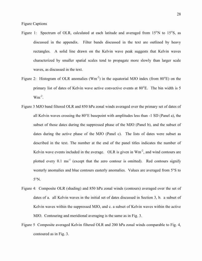
b. Plan View Composites

Figure 6 shows plan view maps of composite OLR and 850 hPa winds for lags -2, 0, and +2

days, with composites for all Kelvin waves and those during the suppressed and active MJO shown

side-by-side to facilitate comparison. Panels a-c include all high amplitude Kelvin waves, panels d-

f include only the subset of Kelvin waves that occurred during the suppressed MJO, and panels g-i

show only the subset of Kelvin waves that occurred during the active MJO. Although composites at

12

other time lags are discussed below, they are not shown for brevity. Panels a-c are discussed first.

The principal wind and OLR anomalies in panels a-c become significantly different from zero

around lag -6 days. At that time, low-level easterly anomalies extend from the eastern side of a

positive OLR anomaly over the central basin westward through a weak negative OLR anomaly. By

lag -4 days, the easterly anomalies intensify along the equator in the region of the positive OLR

anomaly and weaken in the negative OLR anomaly. At lag -3 days, a westerly anomaly develops

along the equator within and to the west of the negative OLR anomaly. This pattern then amplifies

and propagates eastward during subsequent lags. A positive OLR anomaly develops and follows

west of the principal negative OLR anomaly at lag -1 day. Westerlies weaken in this positive OLR

anomaly until the pattern becomes insignificant near lag +4 days. Cyclonic circulations (or gyres,

labeled G on Fig. 6) develop in the vicinity of the active convection on both sides of the equator.

From lag=-2 to 0 days, westerly flow is spread broadly over the region from 10°N to 10°S to the

west of the negative OLR anomaly, but within the negative OLR anomaly, equatorial westerly

anomalies are confined to a much narrower latitude band between the cyclonic gyres. At lag -2

days the southern hemisphere circulation lies to the west behind the northern hemisphere

circulation, but the two circulations become more symmetric across the equator with increasing

time lag. This composite pattern is generally similar to other Kelvin wave composites in that the

zonal wind dominates the low-level flow, with low-level westerly anomalies in active convection

and easterly anomalies often occurring in suppressed convection (e.g., Wheeler et al. 2000; Straub

and Kiladis 2003a). As suggested by the proximity of the gyres to the deep convection, they likely

develop in response to the release of latent heat in the equatorial convective anomaly. In an

analysis of Kelvin waves over the Pacific, Straub and Kiladis (2003b) showed gyres associated with

the forcing of Kelvin waves by incursion of extratropical waves into the equatorial region. The

gyres in the present analysis develop near the equator within the region of deep convection, so they

13

are not likely to be related to those discussed by Straub and Kiladis (2003b). In any case, the

presence of these gyres in the composites suggests that they form systematically and that they

appear with sufficient consistency to be associated with the Kelvin wave OLR anomalies at specific

longitudes. Composite Kelvin filtered winds and OLR based on the same set of dates used to

calculate the composites in panels a-c are nearly identical to these composites (not shown) until lag

2 days (panel c), when stationary and westward-moving features become a significant part of the

pattern (See also Fig. 4a), suggesting that most of the signal relevant to the mean convectively

coupled Kelvin wave lands within the Kelvin band shown in Fig. 1.

Figure 7 a-c shows the composite OLR and 200 hPa winds comparable to the low-level patterns

in Fig. 6 a-c. The wind vectors are drawn on the same length scale as in Fig. 6, and the OLR

patterns are identical because the two composites were averaged over the same set of dates. Outflow

from the strong moist deep convective anomaly dominates the pattern (consistent with Fig. 5a),

although westerly anomalies are collocated with the negative OLR anomaly at lag +2 days. Wind

anomalies curve cyclonically to the northwest and southwest of the active convection at lag +2

days. Along with panel c of Fig. 6, this pattern suggests that the cyclonic structures observed in the

lower levels might tilt westward with increasing height. The outflow from convection occurs in all

directions and is nearly meridional north and south of the negative OLR anomaly (consistent with

Wheeler et al. 2000; Straub and Kiladis 2003b). Easterly and poleward flow dominates a broad

region west of the negative OLR anomaly, whereas westerly and equatorward flow converges into

the equatorial region over the positive OLR anomaly to the east through lag 0 days. This

equatorward flow originates beyond the map domain in the subtropics. The appearance of these

significant patterns of poleward and equatorward flow in the composites suggests that they

consistently appear in association with most convectively coupled Kelvin waves (as in the linear

regression-based composites of Wheeler et al. 2000 and Straub and Kiladis 2003a).

14

Figure 6 d-f shows composite OLR and 850 hPa winds for the subset of Kelvin waves that

occurred during the suppressed MJO. The central OLR and wind anomalies become significantly

different from zero at lag -4 days over Africa (not shown) and the western half of the map domain.

At lag -3 days, easterly anomalies amplify within the positive OLR anomaly over the eastern basin,

with wind anomalies near zero in the region of negative OLR to the west. Westerly anomalies

develop within the negative OLR anomaly at lag=-1 days. Confluence of the zonal wind is most

apparent near the leading edge of the negative OLR anomaly from lags -1 day to +1 day, with the

strongest westerly anomalies collocated with the most negative OLR anomalies. Zonal wind

anomalies dominate the pattern near the equator, consistent with previous analyses of Kelvin waves.

However, off the equator, a pair of broad cyclonic circulations develops on and after lag -1 days in a

pattern that is nearly symmetric across the equator. These circulations remain significantly different

from zero up to lag +6 days and remain largely stationary over the central and eastern basin,

although further plan view composites suggest slow westward-propagation after lag +2 days,

consistent with an n=1 equatorial Rossby wave (Matsuno 1966; Wheeler and Kiladis 1999; Roundy

and Frank 2004). This circulation pattern is apparently left behind as convection coupled to the

Kelvin wave weakens in response to large-scale suppression of convection by the MJO. The gyre

pattern maintains the equatorial westerlies shown in Fig. 6b through lag=+6 days. These gyres are

larger and develop farther west than those that occur in the composite of all Kelvin waves (Fig. 6 a-

c).

Figure 7 d-f shows composite OLR and 200 hPa winds corresponding to Fig. 6 d-f. At lag -2

days, outflow from convection in the negative OLR anomaly curves anticyclonically in the northern

hemisphere. Flow converges toward the equator from the northern hemisphere in the region of

positive OLR anomalies near 100°E, but anomalous northerly flow is also present across the eastern

domain of the composite in the southern hemisphere. From lags -1 days to +1 days, easterly

15

anomalies predominate across the western basin between 10°N and 10°S. Westerly flow to the east

of the negative OLR anomaly is spread much more broadly across the domain from north to south,

and the contributions of meridional winds are much stronger than across the western domain. After

lag +1 days, the equatorial zonal wind anomalies largely dissipate along with the active convection,

leaving behind impulses of poleward and westward flow that radiate away from the diminishing

deep convection toward the northwest and southwest.

Figure 6 g-i shows the composite Kelvin wave pattern of OLR and 850 hPa winds including

only the subset of the waves that occurred during the active MJO. A negative OLR anomaly over

East Africa becomes significant in easterly flow near lag -4 days as it amplifies and progresses

eastward at about 17 ms-1. Positive OLR anomalies precede the negative OLR anomaly to the east

and follow it to the west. After lag -3 days, the anomaly of positive OLR to the east is collocated

with easterly anomalies, especially across the southern hemisphere. Easterly anomalies also

develop within the positive OLR anomaly to the west of the central negative OLR anomaly, but

only after lag +2 days. The low-level flow within the principal negative OLR anomaly is rotational.

Cyclonic flow anomalies extend westward and poleward (especially across the southern

hemisphere) from the negative OLR anomaly. As in the preceding composites of 850 hPa flow,

these anomalies likely develop in response to the release of latent heat in convection coupled to the

Kelvin waves. Comparison of the panels in Fig. 6 suggests that the gyres are smaller and confined

more closely to the equator during the active MJO than during the suppressed MJO. These gyres

are released into the flow near 100°E in Kelvin waves propagating through the active MJO and

farther west, roughly near 85°E during the suppressed MJO. The composites suggest that gyres left

behind by Kelvin waves during the active MJO might be associated with weaker wind anomalies

than those shed during the suppressed MJO, but part of this pattern might be explained by dilution

of the mean signal with distance from the base point since the gyres are released farther east during

16

the active MJO. Comparison with Fig. 4 suggests that these gyres move westward at about 5.3 ms-1,

consistent with an n=1 convectively coupled equatorial Rossby wave (Wheeler and Kiladis 1999;

Roundy and Frank 2004a). The decline of Kelvin wave convection in response to the suppressed

phase of the MJO would explain why the gyres are released farther west during the suppressed MJO

than during the active MJO. The island of Java clearly influences the dissipation of Kelvin wave

convection and the release of the gyres near 100°E, but this work cannot rule out the possibility that

the southern tip of Indian and Sri Lanka might influence the preferred location during the

suppressed MJO. These landmasses create an inhomogeneous background state, apparently

disrupting the organization of convection and causing the gyres to break away from the Kelvin

waves.

Figure 7 g-i shows the composite OLR and 200 hPa winds corresponding to Fig. 6 g-i.

Although zonal wind anomalies dominate the flow on the equator at most time lags, meridional

outflow from the principal region of intense convection and meridional convergence into the region

of suppressed convection on the eastern side of the domain dominates the flow a few degrees away

from the equator. This convergence pattern would enhance the suppressed convective phase of the

Kelvin waves. These meridional wind anomalies extend poleward beyond the map domain.

Southerly flow anomalies continue after the passage of the negative OLR anomaly far to the west of

that anomaly, especially in the northern hemisphere. Wind anomalies curve anticyclonically to the

north and south of the negative OLR anomaly prior to lag 0 and cyclonically to the west of the

negative OLR anomaly after lag 0. This cyclonic curvature at 200 hPa suggests that the cyclonic

gyres shown in Fig 6 h and i might tilt westward with height.

The equatorial negative OLR anomaly is skewed northwestward and southwestward into the

shape of a bow from lags -1 day to +1 day (e.g., Fig. 7h). This OLR pattern is consistent with the

effects of advection of moisture away from low-latitude convection by the upper level winds. The

17

winds relevant to this process are associated with both the MJO and the Kelvin waves. Upper level

wind anomalies associated with the poleward sections of the bow pattern are largely poleward in the

Kelvin wave and largely easterly in the MJO. Moisture exiting at upper-levels from convective

elements embedded in this flow would thus be advected both northwestward and southwestward

away from the equatorial region, and enhanced cloudiness would occur within the stream of

enhanced moisture. A simple scale analysis suggests how advection might explain this bow pattern.

The strongest composite 200 hPa Kelvin band winds in the region of the bow are approximately 4

ms-1. Assuming the life of the bow pattern is about four days as the wave crosses the basin, than

advection by these winds could spread moisture and associated cloudiness more than 12° latitude

from origin points within the central negative OLR anomaly of the wave.

These observations suggest that convectively coupled equatorial waves in the active MJO are

therefore dramatically different in many respects from their shallow-water model counterparts,

which include only oscillations of zonal flow characterized by zero curvature vorticity (e.g.,

Matsuno 1966). These results also suggest that the MJO modulates the behaviors of the Kelvin

waves themselves as well as the development of residual circulations that allow each wave to

continue influencing weather in the Indian basin up to a week after wave passage.

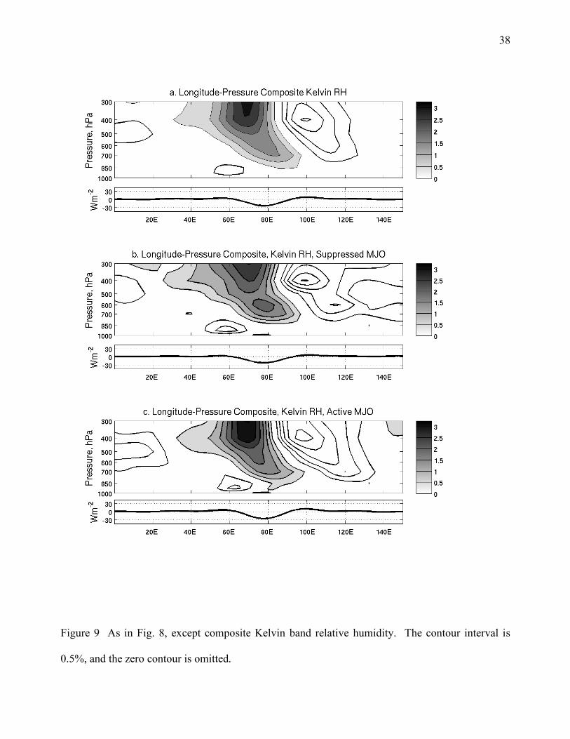
c. Vertical Structure

Figures 8 through 10 show composite Kelvin waves in the longitude-pressure domain for zonal

wind, relative humidity, and temperature, respectively. Only the data filtered for the Kelvin band

are included in these composites to facilitate comparison with previous results. Although not shown

here, the quasi-stationary and westward-moving residual circulations also exhibit vertical structures

that contribute to these variables, but the point of the present analysis is to analyze structures

propagating eastward with the Kelvin waves themselves. Panels a-c of Figs. 8-10 show results

without respect to the MJO, during the suppressed MJO, and during the active MJO (respectively).

18

Figure 3 of Straub and Kiladis (2003b) shows comparable results for Kelvin waves over the Pacific

(without respect to the MJO). Patterns in common across the panels of Figures 8-10 will be

discussed first, followed by the differences between panels b and c. All panels of Figs. 8 and 10

show the vertical “boomerang” structure in winds and temperature described by Wheeler et al.

(2000). Figure 9 shows that this boomerang pattern in winds and temperature occurs along with a

pattern of low-level moistening east of the negative OLR anomaly followed by deep moisture

coincident with and immediately to the west of the negative OLR, in turn followed by a pattern of

moist over dry farther west. A line of confluence of the low-level zonal wind occurs near the

longitude of the OLR minimum at the surface, and this line slopes westward with height to around

400 hPa. West of the OLR minimum, easterly wind anomalies dominate between roughly 200 and

400 hPa with westerly anomalies both above and below the easterly anomalies. Although the

relative humidity data do not resolve moist anomalies above 300 hPa, these easterly anomalies are

frequently observed in association with elevated nimbostratus clouds following the deep convection

in convectively coupled equatorial waves (e.g., Haertel and Kiladis 2004; Kiladis et al. 2005; Mapes

et al. 2006). The composite temperature profiles (Fig. 10) have warm anomalies at low levels and

cold anomalies at the mid to upper levels east of the OLR minimum, with the pattern generally

reversed west of the OLR minimum. The tropospheric temperature pattern suggests low-level

heating east of the negative OLR anomaly, migrating to the mid levels with the onset of deep

convection. Heating then occurs in the elevated nimbostratus cloudiness, with cooling beneath the

nimbostratus region, where rain falls through relatively drier air advected in from the west (see also

Fig. 10a). This general pattern is consistent with progression in cloudiness from shallow cumuli at

the leading edge of the negative OLR anomaly through deep convection immediately east of the

OLR minimum, trailing into elevated nimbostratus along and to the west of the OLR minimum, as

19

described by Johnson et al. (1999), Haertel and Kiladis 2004; Kiladis et al. (2005), Khouider and

Majda (2007) and many others.

Panels b and c of Figs. 8-10 compare the composite structures during the suppressed and active

MJO, respectively. Heavy contours show the 90 percent confidence level for a nonzero difference

between the two MJO phases. Small portions of the composites exhibit significant differences

between signals associated with Kelvin waves during the active and suppressed MJO. For example,

the layer of easterly flow observed west of the OLR minimum between 400 hPa and 100 hPa is

stronger and deeper in Kelvin waves that occur during the suppressed MJO than in Kelvin waves

during the active MJO (Fig. 8 b and c). The vertical gradient through the middle troposphere of the

temperature anomaly pattern west of the negative OLR anomaly is also more amplified during

Kelvin waves in the suppressed MJO relative to Kelvin waves during the active MJO. This pattern

of zonal wind and temperature suggests an amplified nimbostratus stage in cloudiness associated

with Kelvin waves during the suppressed MJO and a weak nimbostratus phase in Kelvin waves that

propagate through the active MJO. These results are generally consistent with the stretched

building-block hypothesis of Mapes et al. (2006), at least with respect to elements of cloudiness

linked specifically to Kelvin waves.

5. Conclusions

Composite average OLR and reanalysis data reveal patterns commonly associated with

convectively coupled Kelvin waves over the tropical Indian Ocean. Further composites show how

these patterns change with the local phase of the MJO. Statistics of the composite Kelvin waves

(Figs. 4-10) are generally similar to those of linear regression-based composites calculated by

Wheeler et al. (2000) and Straub and Kiladis (2003a), with some notable differences. The

composite central negative OLR anomalies associated with Kelvin waves over the Indian Ocean

move eastward at 12.4 ms-1 on average (when calculated without respect to the MJO), 13.9 ms-1

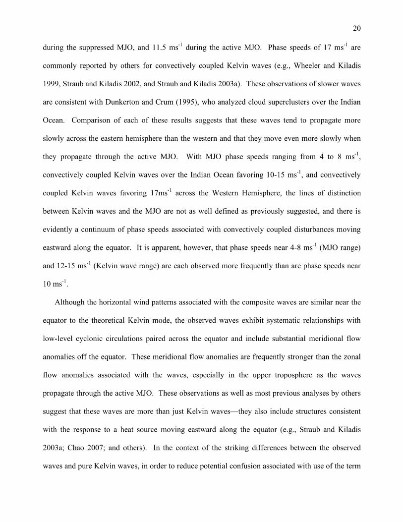
20

during the suppressed MJO, and 11.5 ms-1 during the active MJO. Phase speeds of 17 ms-1 are

commonly reported by others for convectively coupled Kelvin waves (e.g., Wheeler and Kiladis

1999, Straub and Kiladis 2002, and Straub and Kiladis 2003a). These observations of slower waves

are consistent with Dunkerton and Crum (1995), who analyzed cloud superclusters over the Indian

Ocean. Comparison of each of these results suggests that these waves tend to propagate more

slowly across the eastern hemisphere than the western and that they move even more slowly when

they propagate through the active MJO. With MJO phase speeds ranging from 4 to 8 ms-1,

convectively coupled Kelvin waves over the Indian Ocean favoring 10-15 ms-1, and convectively

coupled Kelvin waves favoring 17ms-1 across the Western Hemisphere, the lines of distinction

between Kelvin waves and the MJO are not as well defined as previously suggested, and there is

evidently a continuum of phase speeds associated with convectively coupled disturbances moving

eastward along the equator. It is apparent, however, that phase speeds near 4-8 ms-1 (MJO range)

and 12-15 ms-1 (Kelvin wave range) are each observed more frequently than are phase speeds near

10 ms-1.

Although the horizontal wind patterns associated with the composite waves are similar near the

equator to the theoretical Kelvin mode, the observed waves exhibit systematic relationships with

low-level cyclonic circulations paired across the equator and include substantial meridional flow

anomalies off the equator. These meridional flow anomalies are frequently stronger than the zonal

flow anomalies associated with the waves, especially in the upper troposphere as the waves

propagate through the active MJO. These observations as well as most previous analyses by others

suggest that these waves are more than just Kelvin waves—they also include structures consistent

with the response to a heat source moving eastward along the equator (e.g., Straub and Kiladis

2003a; Chao 2007; and others). In the context of the striking differences between the observed

waves and pure Kelvin waves, in order to reduce potential confusion associated with use of the term

21

“convectively coupled Kelvin waves”, Chao (2007) suggests that these waves be labeled “chimeric

Kelvin waves” because they include “parts of different origin” than pure Kelvin waves.

Consistent with Wheeler et al. (2000), Straub and Kiladis (2003a), and others, low-level

westerly anomalies near the equator tend to be collocated with active convection and easterly

anomalies with suppressed convection. The present analysis further suggests that circulations

linked to the Kelvin waves that are probably associated with the release of latent heat in moist deep

convection coupled to the Kelvin waves. These circulations amplify as the waves cross the Indian

Ocean, but then get left behind the diminishing convective anomalies over the eastern basin,

resulting in residual low-level, low latitude westerly anomalies remaining up to a week after Kelvin

wave passage (Fig. 4). These circulations tend to be released over the central basin during the

suppressed MJO and near 100°E during the active MJO. Equatorial OLR anomalies diminish

rapidly where the circulations become stationary or start moving westward, suggesting that the

circulations become free from the Kelvin waves because convection coupled to the waves begins to

break down. The island of Java (near 100°E) apparently facilitates the disruption of organized

convection coupled to Kelvin waves, so it is a favored location for release of the gyres during the

active MJO.

Composite 200 hPa winds (Fig. 7) suggest that meridional outflow from regions of moist deep

convection forms a major component of the upper level flow associated with Kelvin waves, but this

conclusion is not new. Figure 5 of Wheeler et al. (2000) shows a similar outflow pattern to that

shown in Fig. 7a-c. The present work shows that such outflow patterns tend to be stronger on

average in Kelvin waves that occur during the convectively suppressed or active phases of the MJO

than during periods when the MJO is weak or absent, as suggested by comparison of Figs. 7d-i with

Fig. 7a-c. Comparison of Figures 7e and h suggests that outflow from active convective anomalies

in Kelvin waves that occur during the suppressed MJO tends to be more zonal than in Kelvin waves

22

propagating through the active MJO. Meridional wind anomalies at 200 hPa converge over at least

20 degrees of latitude toward anomalies of suppressed convection, suggesting interaction with the

extra-tropics, especially during the active MJO. Meridional outflow from the centers of deep

convection in Kelvin waves in the active MJO apparently cooperates with MJO-induced flow to

advect upper-level moisture and cloudiness northwestward and southwestward, generating the bow

pattern seen in Fig. 6h. This bow pattern is not observed in Kelvin waves propagating through the

suppressed convective phase of the MJO.

Vertical structures of wind and temperature anomalies associated with Kelvin waves depend

significantly on the phase of the MJO through which they propagate. In particular, these structures

suggest that the elevated nimbostratus stage of cloudiness in Kelvin waves is weak when the waves

occur during the active MJO. In contrast, the nimbostratus stage is deeper and more amplified in

Kelvin waves during the suppressed MJO. These results support the general premise of the

stretched building block hypothesis for evolution of cloudiness associated with waves propagating

through the MJO suggested by Mapes et al. (2006), because the spatial coverage and strength of the

stratiform stage of Kelvin wave cloudiness is reduced near the most active MJO convection and

enhanced when Kelvin waves propagate through the suppressed MJO.

Since these Kelvin waves are present during most MJO events, any hierarchical model for the

MJO should include these patterns of behavior and acknowledge that these patterns evolve

differently during different phases of the MJO. The author is presently applying regression models

to analyze modulation of Kelvin waves and other disturbances by the MJO. Results of this work

will likely reveal changes in wave structures across a continuum of MJO phases instead of just the

active and suppressed convective phases analyzed here. Additionally, the presence of the residual

cyclonic flow anomalies left behind by Kelvin waves raises questions about whether Kelvin waves

might help generate precursors for tropical cyclones over the Indian Ocean. This possibility was

23

not addressed by Frank and Roundy (2006) or by Bessafi and Wheeler (2006) in their analyses of

relationships between convectively coupled waves and tropical cyclogenesis.

Acknowledgements: This work was made possible through start-up funds provided by the

Research Foundation of the State University of New York. Comments of three anonymous

reviewers dramatically improved the manuscript. Discussions with Ademe Mekonnen; Joseph

Kravitz, and George Kiladis were critical to this work. I appreciate the contributions of free OLR

and reanalysis data provided by the NOAA ESRL.

24

Appendix

The power spectrum of OLR shown in Fig. 1 was calculated and normalized using a method

comparable to that of Wheeler and Kiladis (1999) and Roundy and Frank (2004a), except that cross-

equatorial symmetric filters were not included in the calculations. Spectra were calculated for OLR

data at each latitude, by breaking the entire longitude-time dataset for a given latitude up into many

overlapping 96-day time windows. Each window was tapered at the ends in time by multiplying by

cosine bells. A Fourier transform in longitude was applied to each of the segments, followed by

another transform in time. Spectral power was obtained by multiplying the result by its complex

conjugate. The spectral estimate for each latitude is just the average of the spectra calculated from

all of the windows at that latitude. The mean spectrum was calculated by averaging the results

across 15°N to 15°S. The mean spectrum was then normalized by dividing by a smoothed

background, which was generated by smoothing the spectrum 40 times in wavenumber and 40 times

in frequency (similar to the smoothing method applied by Wheeler and Kiladis 1999, but with

different smoothing rates).

25

References

Bessafi, M., and M. Wheeler, 2006: Modulation of south Indian Ocean tropical cyclones by the

Madden-Julian Oscillation and convectively coupled waves. Mon. Wea. Rev., 134, 638-656.

Chang, C.-P., and H. Lim, 1988: Kelvin Wave-CISK: A possible mechanism for the 30-50 day

oscillations. J. Atmos. Sci., 45, 1709-1720.

Chao, W. C., 2007: Chimeric equatorial waves as a better descriptor for “Convectively coupled

equatorial waves”. J. Meteor. Soc. Japan, 85, 521-524.

Cho, H.-R., K. Fraedrich, and J. T. Wang, 1994: Cloud clusters, Kelvin wave-CISK, and the

Madden-Julian Oscillation in the equatorial troposphere. J. Atmos. Sci., 51, 68-76.

Dickinson, M., and J. Molinari, 2002: Mixed Rossby-gravity waves and western Pacific tropical

cyclogenesis. Part I: Synoptic evolution. J. Atmos. Sci., 59, 2183-2196.

Dunkerton, T. J., and F. X. Crum 1995: Eastward propagating ~2 to 15-day equatorial convection and its

relation to the tropical intraseasonal oscillation. J. Geophys. Res., 100, 25781-25790.

Ferreira, R. N., W. H. Schubert, and J. J. Hack, 1996: Dynamical aspects of twin tropical cyclones

associated with the Madden-Julian Oscillation. J. Atmos. Sci., 53, 929-945.

Frank, W. M., and P. E. Roundy, 2006: The role of tropical waves in tropical cyclogenesis. Mon.

Wea. Rev., 134, 2397-2417.

Haertel, P., and G. N. Kiladis, 2004: Dynamics of 2-day equatorial waves. J. Atmos. Sci., 61,

2707-2721.

Hendon, H. H., and B. Liebmann, 1991: The structure and annual variation of antisymmetric

fluctuations of tropical convection and their association with Rossby-gravity waves. J.

Atmos. Sci., 51, 2225-2237.

Hendon, H.H., B. Liebmann, and J. D. Glick, 1998: Oceanic Kelvin waves and the Madden-Julian

Oscillation. J. Atmos. Sci., 55, 88-101.

26

Johnson, R. H., T. M. Richenbach, S. A. Rutledge, P. E. Ciesielski, and W. H. Schubert, 1999:

Trimodal characteristics of tropical convection. J. Climate, 12, 2397-2407.

Kalnay, E., M. Kanamitsu, R. Kistler, W. Collins, D. Deaven, L. Gandin, M. Iredell, S. Saha, G.

White, J. Woollen, Y. Zhu, M. Chelliah, W. Ebisuzaki, W. Higgins, J. Janowiak, K. C. Mo,

C. Ropelewski, J. Wang, A. Leetmaa, R. Reynolds, R. Jenne, and D. Joseph, 1996: The

NCEP/NCAR 40-year reanalysis project. Bull. Amer. Meteor. Soc., 77, 437-471.

Kiladis, G. N., K. H. Straub, and P. T. Haertel, 2005: Zonal and vertical structure of the Madden

Julian Oscillation. J. Atmos. Sci., 62, 2790-2809.

Khouider, B., and A. J. Majda, 2007: A simple multicloud parameterization for convectively

coupled tropical waves. Part II: Ninlinear Simulations. J. Atmos. Sci., 64, 381-400.

Liebmann, B., H. H. Hendon, and J. D. Glick, 1994: The relationship between tropical cyclones of

the western Pacific and Indian Oceans and the Madden-Julian Oscillation. J. Meteor. Soc.

Japan, 72, 401-412.

Liebmann, B., and C. A. smith, 1996: Description of a complete (interpolated) outgoing longwave

radiation dataset. Bull. Amer. Meteor. Soc., 77, 1275-1277.

Madden, R. A., and P. R. Julian, 1994: Observations of the 40-50 day tropical oscillation—A

review. Mon. Wea. Rev., 122, 814-837.

Majda, A. J., B. Khouider, G. N. Kiladis, K. H. Straub, and M. G. Shefter, 2004: A model for

convectively coupled tropical waves: Nonlinearity, rotation, and comparison with

observations. J. Atmos. Sci., 61, 2188-2205.

Maloney, E. D., and D. L. Hartmann, 2001: The Madden-Julian Oscillation, barotropic dynamics,

and North Pacific tropical cyclone formation. J. Atmos. Sci., 58, 2545-2558.

Mapes, B., S. Tulich, J. Lin, and P. Zuidema, 2006: The mesoscale convective life cycle: building

block or prototype for large-scale tropical waves? Dyn. Atmos. Oceans, 42, 3-29.

27

Matsuno, T., 1966: Quasi-geostrophic motions in the equatorial area. J. Meteor. Soc. Japan, 44,

25-43.

Nakazawa, T., 1988: Tropical super clusters within intraseasonal variations over the western

Pacific. J. Meteor. Soc. Japan, 66, 823-839.

Roundy, P. E., and G. N. Kiladis, 2006: Observed relationships between oceanic Kelvin waves and

atmospheric forcing. J. Climate, 19, 5253-5272.

Roundy, P. E., and W. M. Frank, 2004a: A climatology of waves in the equatorial region. J.

Atmos. Sci., 61, 2105-2132.

Roundy, P. E., and W. M. Frank, 2004b: Effects of low-frequency wave interactions on

intraseasonal oscillations. J. Atmos. Sci., 61, 3025-3040.

Straub, K. H., and G. N. Kiladis, 2002: Observations of a convectively coupled Kelvin wave in the

eastern Pacific ITCZ. J. Atmos. Sci., 59, 30-53.

Straub, K. H., and G. N. Kiladis, 2003a: The observed structure of convectively coupled Kelvin

waves: Comparison with simple models of coupled wave instability. J. Atmos. Sci., 60,

1655-1668.

Straub, K. H., and G. N. Kiladis, 2003b: Extratropical forcing of convectively coupled Kelvin

waves during Austral winter. J. Atmos. Sci., 60, 526-543.

Takayabu, Y. N., and Murakami, M., 1991: The structure of super cloud clusters observed in 1-20

June 1986 and their relationship to easterly waves. J. Meteor. Soc. Japan, 69, 105-125.

Wheeler, M., and G. N. Kiladis, 1999: Convectively coupled equatorial waves: Analysis of clouds

and temperature in the wavenumber-frequency domain. J. Atmos. Sci., 56, 374-399.

Wheeler, M., G. N. Kiladis, and P. J. Webster, 2000: Large-scale dynamical fields associated with

convectively coupled equatorial waves. J. Atmos. Sci., 57, 613-640.

Wilks, D. S., 2006: Statistical Methods in the Atmospheric Sciences. Academic Press. 627 pp.

28

Figure Captions

Figure 1: Spectrum of OLR, calculated at each latitude and averaged from 15°N to 15°S, as

discussed in the appendix. Filter bands discussed in the text are outlined by heavy

rectangles. A solid line drawn on the Kelvin wave peak suggests that Kelvin waves

characterized by smaller spatial scales tend to propagate more slowly than larger scale

waves, as discussed in the text.

Figure 2: Histogram of OLR anomalies (Wm-2) in the equatorial MJO index (from 80°E) on the

primary list of dates of Kelvin wave active convective events at 80°E. The bin width is 5

Wm-2.

Figure 3 MJO band filtered OLR and 850 hPa zonal winds averaged over the primary set of dates of

all Kelvin waves crossing the 80°E basepoint with amplitudes less than -1 SD (Panel a), the

subset of those dates during the suppressed phase of the MJO (Panel b), and the subset of

dates during the active phase of the MJO (Panel c). The lists of dates were subset as

described in the text. The number at the end of the panel titles indicates the number of

Kelvin wave events included in the average. OLR is given in Wm-2, and wind contours are

plotted every 0.1 ms-1 (except that the zero contour is omitted). Red contours signify

westerly anomalies and blue contours easterly anomalies. Values are averaged from 5°S to

5°N.

Figure 4: Composite OLR (shading) and 850 hPa zonal winds (contours) averaged over the set of

dates of a. all Kelvin waves in the initial set of dates discussed in Section 3, b. a subset of

Kelvin waves within the suppressed MJO, and c. a subset of Kelvin waves within the active

MJO. Contouring and meridional averaging is the same as in Fig. 3.

Figure 5 Composite averaged Kelvin filtered OLR and 200 hPa zonal winds comparable to Fig. 4,

contoured as in Fig. 3.

29

Figure 6 Plan view maps of composite averaged Kelvin filtered OLR and 850 hPa winds.

Averages were made for panels a-c over the same set of dates used in Fig. 3a, panels d-f

used the same set of dates as in Fig. 3b, and g-i used the same set of dates as in Fig. 3c.

Winds are plotted only if either the zonal or meridional components are significantly

different from zero. OLR contours are the same as in Figs 3-5, plotted every 5 Wm-2. The

strongest wind anomalies across the set of panels are near 1.2 ms-1.

Figure 7 Composite Kelvin OLR and 200 hPa wind anomalies for the set of Kelvin waves included

in Fig. 6, contoured as in Fig. 6. The strongest wind anomalies across the set of panels is

near 2 ms-1.

Figure 8 Composite Kelvin band zonal wind (ms-1) averaged from 5°N to 5°S for a, the set of all

active convective phases of Kelvin waves with OLR anomalies less than one standard

deviation below the mean, b, the subset of the events in panel a that occurred within 5 days

before or after the OLR maxima of suppressed convective phases of the MJO, and c, the set

of Kelvin waves within 5 days of the OLR minima of the active convective phases of the

MJO. Shading begins at 0.1 ms-1, with additional contours every 0.1 ms-1. The heavy line

outlines where anomalies exceed the 95 percent level for difference between panels b and c.

Figure 9 As in Fig. 8, except composite Kelvin band relative humidity. The contour interval is

0.5%, and the zero contour is omitted.

Figure 10 As in Fig. 8, except composite Kelvin band temperature (°C).

30

Figure 1: Spectrum of OLR, calculated at each latitude and averaged from 15°N to 15°S, as

discussed in the appendix. Filter bands discussed in the text are outlined by heavy

rectangles. A solid line drawn on the Kelvin wave peak suggests that Kelvin waves

characterized by smaller spatial scales tend to propagate more slowly than larger scale

waves, as discussed in the text.

31

Figure 2: Histogram of OLR anomalies (Wm-2) in the equatorial MJO index (from 80°E) on the

primary list of dates of Kelvin wave active convective events at 80°E. The bin width is 5

Wm-2.

32

Figure 3 MJO band filtered OLR and 850 hPa zonal winds averaged over the primary set of dates of

all Kelvin waves crossing the 80°E basepoint with amplitudes less than -1 SD (Panel a), the subset of those dates during the suppressed phase of the MJO (Panel b), and the subset of dates during the active phase of the MJO (Panel c). The lists of dates were subset as described in the text. The number at the end of the panel titles indicates the number of Kelvin wave events included in the average. OLR is given in Wm-2, and wind contours are plotted every 0.1 ms-1 (except that the zero contour is omitted). Red contours signify westerly anomalies and blue contours easterly anomalies. Values are averaged from 5°S to 5°N.

33

Figure 4 Composite OLR (shading) and 850 hPa zonal winds (contours) averaged over the set of

dates of a. all Kelvin waves in the initial set of dates discussed in Section 3, b. a subset of Kelvin waves within the suppressed MJO, and c. a subset of Kelvin waves within the active MJO. Contouring and meridional averaging is the same as in Fig. 3.

34

Figure 5 Composite averaged Kelvin filtered OLR and 200 hPa zonal winds comparable to Fig. 4,

contoured as in Fig. 3.

35

Figure 6 Figure 6 Plan view maps of composite averaged Kelvin filtered OLR and 850 hPa winds. Averages were made for panels a-c over the same set of dates used in Fig. 3a, panels d-f used the same set of dates as in Fig. 3b, and g-i used the same set of dates as in Fig. 3c. Winds are plotted only if either the zonal or meridional components are significantly different from zero. OLR contours are the same as in Figs 3-5, plotted every 5 Wm-2. The strongest wind anomalies across the set of panels are near 1.2 ms-1.

36

Figure 7 Composite Kelvin OLR and 200 hPa wind anomalies for the set of Kelvin waves included

in the corresponding panels of Fig. 6, contoured as in Fig. 6. The strongest wind anomalies

across the set of panels are near 2 ms-1.

37

Figure 8 Composite Kelvin band zonal wind (ms-1) averaged from 5°N to 5°S for a, the set of all active convective phases of Kelvin waves with OLR anomalies less than one standard deviation below the mean, b, the subset of the events in panel a that occurred within 5 days before or after the OLR maxima of suppressed convective phases of the MJO, and c, the set of Kelvin waves within 5 days of the OLR minima of the active convective phases of the MJO. Shading begins at 0.1 ms-1, with additional contours every 0.1 ms-1. The heavy line outlines where anomalies exceed the 95 percent level for difference between panels b and c.

38

Figure 9 As in Fig. 8, except composite Kelvin band relative humidity. The contour interval is

0.5%, and the zero contour is omitted.

39

Figure 10 As in Fig. 8, except composite Kelvin band temperature (°C). The contour interval is

0.05°C, and the zero line is omitted.