KELVIN-HELMHOLTZ INSTABILITY BY...

II International Conference on Particle-based Methods - Fundamentals and ApplicationsPARTICLES 2011

E. Onate and D.R.J. Owen (Eds)

KELVIN-HELMHOLTZ INSTABILITY BY SPH

M. S. Shadloo∗, M. Yildiz†

Faculty of Engineering and Natural Sciences, Advanced Composites & Polymer ProcessingLaboratory, Sabanci University, 34956 Tuzla, Istanbul, Turkey.

∗e-mail: [email protected], www.msshadloo.com†e-mail: [email protected]

Key words: Smoothed Particle Hydrodynamics (SPH), Shear flow, Two-Phase flow,Interfacial flows, Surface tension, Kelvin-Helmholtz Instability (KHI).

Abstract. In this paper, we have modeled the Kelvin-Helmholtz Instability (KHI) prob-lem of an incompressible two-phase immiscible fluid in a stratified inviscid shear flow withinterfacial tension using Smoothed Particle Hydrodynamics (SPH) method. The time de-pendent evolution of the two-fluid interface over a wide range of Richardson number (Ri)and for three different density ratios is numerically investigated. The simulation resultsare compared with analytical solutions in the linear regime. It was observed that theSPH method requires a Richardson number lower than unity (i.e., Ri ∼= 0.8) for the onsetof KHI, and that the artificial viscosity plays a significant role in obtaining physicallycorrect simulation results that are in agreement with analytical solutions. The numericalalgorithm presented in this work can easily handle a two-phase fluid flow with variousdensity ratios.

1 INTRODUCTION

Flow instability at the interface between two horizontal parallel streams of different ve-locities and densities, with the heavier fluid at the bottom, is called the Kelvin-HelmholtzInstability (KHI). The KHI is induced by either velocity shear within a continuous fluidor a sufficiently large velocity difference across the interface of a multiphase fluid. Theinstability kicks in when the destabilizing effect of shear across the interface overcomesthe stabilizing effect of stratification due to gravity and/or surface tension if it exists. TheKHI manifests itself as a row of horizontal eddies (in the form of waves) aligned acrossthe interface. These eddies or waves are referred to as main billows. There are severalwell-known natural situations where the KHI can be observed such as wind blowing overthe ocean or water surface, a meteor entering the Earth’s atmosphere, the interface be-tween the tails of comets and solar wind, or the interface between a liquid layer and acompressible gas, among others.

1

M. S. Shadloo, M. Yildiz

The Kelvin-Helmholtz instability problem was solved first for the ideal case of inviscidand incompressible fluids in 1871 by Lord Kelvin. It has been studied both theoretically [1]and experimentally [2], as well as numerically [3, 4].

Smoothed Particles Hydrodynamics (SPH) is one of the most successful Lagrangianmethods which was introduced separately by Gingold and Monaghan and Lucy in 1977initially to simulate astrophysical problems. Due to its flexibility and capability of model-ing complex engineering problems, the SPH method has been extensively used for solvinga wide variety of problems [5, 6]. As well, there are some recently reported works whichhave been conducted to investigate the feasibility and the ability of the SPH method tocapture the physics behind the KHI [7, 8].

The aim of this work is to simulate the KHI by using a Weakly Compressible SPH(WCSPH) method, thereby showing the ability of the SPH technique to capture thishydrodynamic instability for various density ratios. The current presentation differs fromearlier works in the following aspects: the previously reported relevant works treated thefluid to be compressible whereas here it is treated as an incompressible liquid. Unlike otherpertinent SPH papers, this paper systematically examines the effects of the stabilizingparameters (e.g. surface tension (σ) and stratifying body force (∆ρg)) individually orconcurrently on the occurrence of the KHI for a wide range of Ri numbers and threedensity ratios.

2 SMOOTHED PARTICLE HYDRODYNAMICS

SPH is a Lagrangian particle-based method which has been extensively used over adecade for solving partial differential equations (thermo mechanical balance laws inte-grated with relevant constitutive equations) for both fluids and solids dynamic problems.Incomparison to mesh-dependent approaches, the SPH method significantly facilitates thehandling of the problems with free or interfacial surface, whose locations are priori un-known and have to be computed during the solution of the problem since the position ofparticles determine the final configuration of the flow domain. Therefore, it is a particu-larly powerful tool to study multiphase fluid flow problems.

The term particles merely refers to movable points that represent fluid elements in threedimensional space, and each particle is associated with mass, density, velocity and otherrelevant hydrodynamics properties. In another way of saying, the continuum under theconsideration is discretized into finite number of field points which are known as particles.Field variables carried by each particle are calculated through an interpolation (weighting,smoothing, kernel) function, W (rij, h) from those of surrounding neighbor particles. Here,rij is the magnitude of the distance vector (~rij = ~ri-~rj) between the particle of interesti (an interpolated particle) and its neighboring particles j (neighbors of the interpolatedparticle), and h is called smoothing length, which is an important input parameter thatcontrols the number of active neighbor particles within the support domain of smoothingfunction. Here, ~ri and ~rj are the position vectors for particles i and j, respectively. Theweighting function should have the following attributes; the normalization, the Dirac-delta

2


function, the compactness, and spherically symmetric even function properties. Due tothe compactness property, W (rij, h) = 0 when rij > h, in computations, a given particleinteracts with only its nearest neighbors contained within the radius of support domainh.

For an arbitrary function (scalar (A), vectorial (~A), or tensorial (A), the kernel ap-proximation in the form of the integral representation can be written as

A(~ri) ∼= 〈A(~ri)〉 ≡∫

Space

A(~rj)W (rij, h)d3~rj. (1)

where the angle bracket 〈〉 denotes the kernel approximation.In the SPH method, it is common practice to replace the integral operation with a

summation over all the particles within the support domain of the kernel function (i.e.rij < h ). In what follows, one can write

Ai = A(~ri) =1

ψi

∑

j

AjWij (2)

where we have used a concise notation (i.e. W (rij, h) = Wij), and the differential volumeelement d3~rj is approximated by the reciprocal of the number density ψi, which is definedfor the particle i as

ψi =∑

j

Wij, (3)

By using a differentiable kernel, the spatial derivative of the function A evaluatedat the location of particle i can be simply reduced to an ordinary differentiation of theinterpolant function Wij with respect to the particle i times the volume and the fieldvariables of neighbor particles. It is due to this analytical approximation that the SPHmethod does not require a grid. For example, one of the widely used SPH gradientdiscretization scheme of the field A can be written in the form of

∇iAi = ∇~riA(~ri) =1

ψi

∑

j

(Aj − Ai)∇iWij. (4)

where ∇~riA(~ri) or in a concise notation ∇iAi denotes the spatial derivative of the fieldA with respect to ith particle coordinates. Since the kernel function determines the extentof the interaction between the particle of interest and its neighbors, its choice is related tothe accuracy, efficiency, and stability of the resulting algorithm. In this work, the quintickernel based on the fifth-order spline function is adopted [9].

3


2.1 Governing Equations

The governing equations used to solve the fluid problems in this article are the massand linear momentum balance equations which are expressed in the Lagrangian form andgiven in the direct notation as

dρ

dt= −ρ∇ · ~v, (5)

ρd~v

dt= −∇p + ρ~g + ~F

σ, (6)

where p is the pressure, ~v is the fluid velocity, and ~Fσ

denotes a force per unit volumeexerted on the fluid-fluid interface due to surface tension. Here, it should be pointedout that in reality, the surface tension force on the fluid-fluid interface is a surface force(i.e., force per unit area). For the sake of computational efficiency and simplifications, wehere have followed a common practice whereby the surface tension force per unit area isincluded in the momentum balance equation as the force per unit volume. As written ineq.(12),this volume force is proportional to product of the interface gradient (gradient ofthe color field used to distinguish two fluids) and the surface curvature. This approachis referred to as the continuum surface force (CSF) formulation and is widely used inmodeling surface tension force of multiphase fluid flows. Also, it should be noted thatdue to the inviscid fluid assumption, the linear momentum balance equation does nothave a viscous force term.

In the WCSPH method, for enforcing the incompressibility condition, the density canbe evolved either using eq. (5) in combination with eq. (4) or directly utilizing the numberdensity approach as given in eq. (7).

ρi = miψi (7)

As for the balance of linear momentum equation, the acceleration term can be dis-cretized in the general form of

~ai =1

mi

~Fi, (8)

where ~Fi is the total force acting on the particle i, which can be written in the discreteform as

~Fi = mi~g + ~Fσ

i −∑

j

[

(piψ2

i

+pjψ2

j

) + Πij

]

∇iWij. (9)

Here, the first term in the summation sign (pi/ψ2i + pj/ψ

2j ) is the discretized form of

the pressure gradient force and Πij is artificial viscosity.

4


The artificial viscosity term is included in the current model in order for circumventingnumerical instabilities due to the meshless nature of the SPH method. This term intro-duces some numerical diffusion into the model, thus preventing non-physical oscillations.There are various forms of artificial viscosity terms in SPH literature. In this work, wehave implemented the one suggested by Monaghan in [10] in the form of

Πij = − 8µij(~vij ·~rij)

ψiψj(r2ij + ǫh2

m)(10)

where ~vij = ~vi − ~vj, ~rij = ~ri − ~rj, hm =hi+hj

2, ǫ ≈ 0.0001 is introduced to prevent

singularity when rij = 0 and µij is harmonic average of µi and µj defined by

µij =2

1µi

+ 1µj

, (11)

where µi = 18αhiciρi in which c is sound speed and α is the artificial viscosity constant.

In accordance with the continuum surface force (CSF) formulation, the surface tensionforce term in eq.(9) is formulated as

~Fσ

i = σiκi~niδs, (12)

where κi is the interface curvature, and ~ni is the unit vector normal to interface andδs is the interface dirac delta function(δs = |∇C|).

The unit vector normal to the fluid-fluid interface ~ni is

~ni =∇iC i

|∇iCi|. (13)

where ∇iC i is computed as.

∇iC i =∑

j

Cji

ψij

∇iWij. (14)

where ψij = (ψi + ψj)/2 and Cji = Cj − Ci.Finally, the interface curvature κi is calculated from

κi =∑

j

1

ψij

~nij · ∇iWij, (15)

where ~nij = ~ni − ~nj.

5


2.2 Time Integration

In order to increment the time-steps in the SPH algorithm, we have used a VelocityVerlet predictor corrector method [10]. This technique is an explicit time integrationscheme, and is relatively simple to implement. The time integration scheme starts with thepredictor step to compute the intermediate particle positions based on current particles’velocities as follow

~rn+ 1

2

i = ~rni +

∆t

2~vn

i . (16)

where n is the temporal index.Afterward, new densities for each particles are calculated from eq.(3) and eq.(7) at

current intermediate particle positions. Since fluid is assumed weakly compressible, theartificial equation of state of the form

p− po = c2(ρ− ρo), (17)

is used to compute new pressure values at current particle positions. This state equationenforces the incompressibility condition on the flow such that a small variation in densityproduces a relatively large change in pressure hence preventing the dilatation of the fluid.Here, c is artificial sound velocity and the subscript o denotes the reference condition. Thespeed of sound for each particle must be chosen carefully to ensure that the fluid is veryclosely incompressible. In this work, upon selecting the sound speed twenty times largerthan the maximum fluid velocity, the density variation is limited to one percent. Havingcomputed the acceleration of each particle from eq.(8) using the current pressure andvelocity values, one can obtain the velocity of new time-step through the time integrationas

~vn+1i = ~vn

i + ~an+ 1

2

i ∆t. (18)

Finally, the position of each particle is corrected at the new time-step based on thisvelocity. It is to be noted that in the SPH method, the order of particles affects theaccuracy of interpolations for gradient and Laplacian computations. Therefore, for thecomputational stability and accuracy, it is preferable to move the SPH particles in amore orderly fashion, which can be achieved through using the XSPH technique proposedby Monaghan et.al [10]. The XSPH method includes the contribution from neighboringparticles, thereby causing a fluid particle to move with an average velocity

~rn+1i = ~r

n+ 1

2

i +∆t

2~v

∗n+1i , (19)

where ~v∗n+1i is the XSPH-averaged new velocity by the correction factor of 0.1.

6


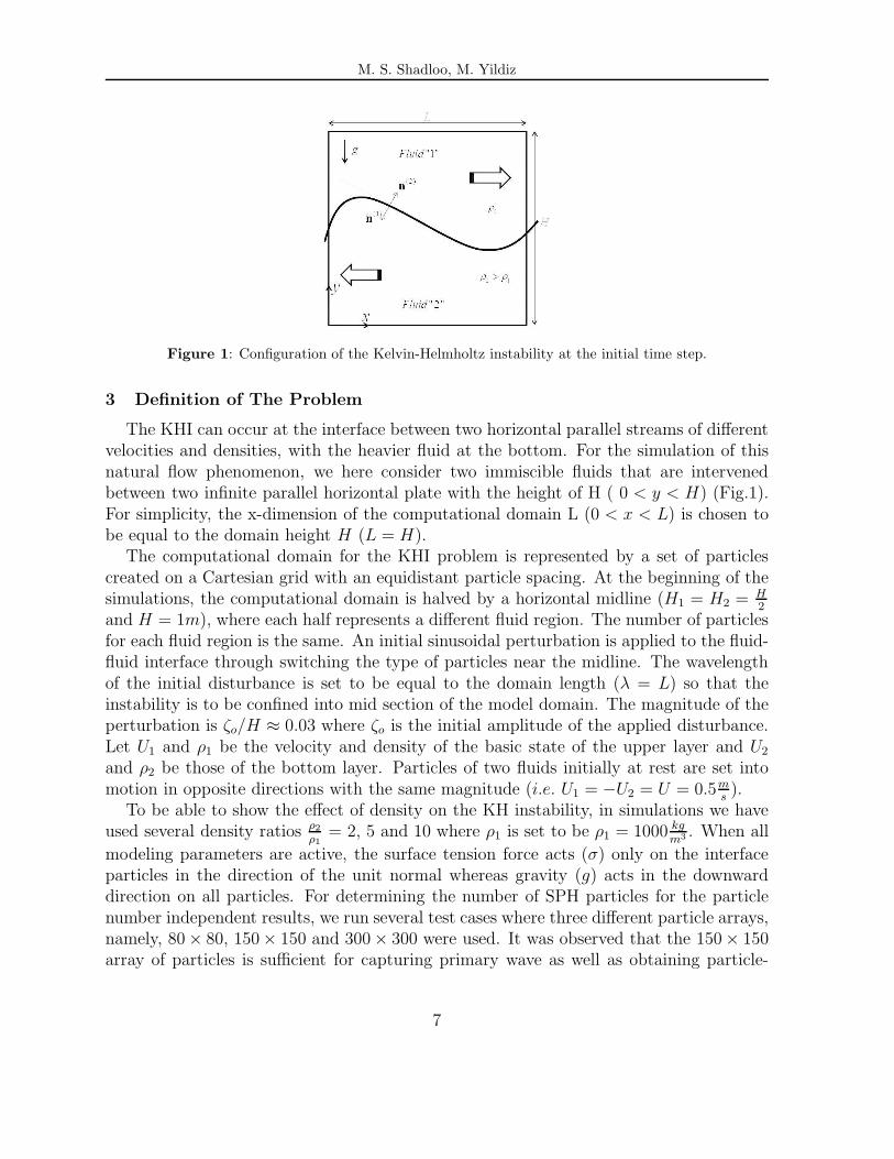
Figure 1: Configuration of the Kelvin-Helmholtz instability at the initial time step.

3 Definition of The Problem

The KHI can occur at the interface between two horizontal parallel streams of differentvelocities and densities, with the heavier fluid at the bottom. For the simulation of thisnatural flow phenomenon, we here consider two immiscible fluids that are intervenedbetween two infinite parallel horizontal plate with the height of H ( 0 < y < H) (Fig.1).For simplicity, the x-dimension of the computational domain L (0 < x < L) is chosen tobe equal to the domain height H (L = H).

The computational domain for the KHI problem is represented by a set of particlescreated on a Cartesian grid with an equidistant particle spacing. At the beginning of thesimulations, the computational domain is halved by a horizontal midline (H1 = H2 = H

2

and H = 1m), where each half represents a different fluid region. The number of particlesfor each fluid region is the same. An initial sinusoidal perturbation is applied to the fluid-fluid interface through switching the type of particles near the midline. The wavelengthof the initial disturbance is set to be equal to the domain length (λ = L) so that theinstability is to be confined into mid section of the model domain. The magnitude of theperturbation is ζo/H ≈ 0.03 where ζo is the initial amplitude of the applied disturbance.Let U1 and ρ1 be the velocity and density of the basic state of the upper layer and U2

and ρ2 be those of the bottom layer. Particles of two fluids initially at rest are set intomotion in opposite directions with the same magnitude (i.e. U1 = −U2 = U = 0.5m

s).

To be able to show the effect of density on the KH instability, in simulations we haveused several density ratios ρ2

ρ1

= 2, 5 and 10 where ρ1 is set to be ρ1 = 1000 kg

m3 . When all

modeling parameters are active, the surface tension force acts (σ) only on the interfaceparticles in the direction of the unit normal whereas gravity (g) acts in the downwarddirection on all particles. For determining the number of SPH particles for the particlenumber independent results, we run several test cases where three different particle arrays,namely, 80 × 80, 150× 150 and 300 × 300 were used. It was observed that the 150× 150array of particles is sufficient for capturing primary wave as well as obtaining particle-

7


independent solutions.

4 RESULTS

For unstable situations, the analytical non-dimensional growth rate Ge in the linearregime can be written as [11]

Ge = Im(ω) =2π

√ρ1ρ2

ρ1 + ρ2

√1 −Ri. (20)

where Ri is the dimensionless Richardson number

Ri =ρ1 + ρ2

kρ1ρ2(U1 − U2)2

(

g(ρ2 − ρ1) + k2σ)

. (21)

For numerical investigation, the numerical growth rate Gn is calculated in the form of

Gn =ζ/ζo − 1

t∗, (22)

where ζ is the amplitude of the disturbance at time t and t∗ is the dimensionless time.

t∗ =t |U2 − U1|

H, (23)

where t is real time and H is domain height.To be able to compare the analytical growth rate in eq.(20) with the numerical one in

eq.(22), (because eq.(20) is only valid for the linear regime), ζ and t∗ are calculated whenthe wave amplitude reaches to 10 percentage of the domain height (ζ ∼= 0.1H).

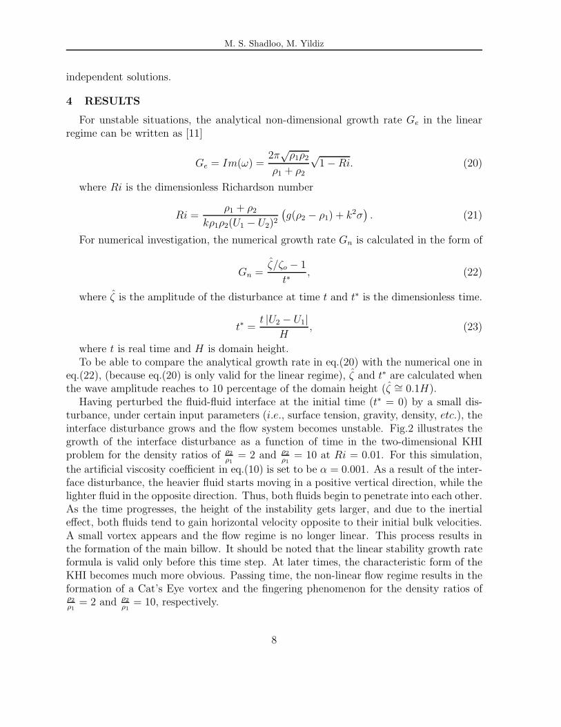
Having perturbed the fluid-fluid interface at the initial time (t∗ = 0) by a small dis-turbance, under certain input parameters (i.e., surface tension, gravity, density, etc.), theinterface disturbance grows and the flow system becomes unstable. Fig.2 illustrates thegrowth of the interface disturbance as a function of time in the two-dimensional KHIproblem for the density ratios of ρ2

ρ1

= 2 and ρ2

ρ1

= 10 at Ri = 0.01. For this simulation,

the artificial viscosity coefficient in eq.(10) is set to be α = 0.001. As a result of the inter-face disturbance, the heavier fluid starts moving in a positive vertical direction, while thelighter fluid in the opposite direction. Thus, both fluids begin to penetrate into each other.As the time progresses, the height of the instability gets larger, and due to the inertialeffect, both fluids tend to gain horizontal velocity opposite to their initial bulk velocities.A small vortex appears and the flow regime is no longer linear. This process results inthe formation of the main billow. It should be noted that the linear stability growth rateformula is valid only before this time step. At later times, the characteristic form of theKHI becomes much more obvious. Passing time, the non-linear flow regime results in theformation of a Cat’s Eye vortex and the fingering phenomenon for the density ratios ofρ2

ρ1

= 2 and ρ2

ρ1

= 10, respectively.

8


(I)

(II)

Figure 2: Time evolution of the interface in the two-dimensional KHI problem with the density ratios ofρ2

ρ1

= 2 and ρ2

ρ1

= 10, and the Ri = 0.01; (a)t∗ = 1.0, (b)t∗ = 2.0, (c)t∗ = 3.0, (d)t∗ = 4.0; (I) particle

distributions and (II) velocity vectors.

9


In the simulation with the density ratio of 2, both fluids have relatively close inertialforces, and therefore, the vortex is not advected significantly by fluid streams. Conse-quently, as the simulation progresses, the flow circulation forms the Cat’s Eye shape. Onthe other hand, due to the fact that there exists a relatively large difference in the inertialforces between the upper and the lower fluid layers for the density ratio of 10 , and theheavier fluid at the bottom of the modeling domain has a greater inertial force than thelighter fluid at the top, the flow circulation is advected faster in the flow direction of theheavier fluid whereby it leaves the flow domain through the left side and re-enters it fromthe right side. Accordingly, the translational motion of the flow circulation along the in-terface brings about the elongation of the crest of the wave, or the fingering phenomenon.

From eq.(20) it is also notable that for a given density ratio, the Ri number is theonly parameter that controls the stability of the two fluid system in the KHI phenomena.Towards this end, it is important to determine the critical value for this number, whichdefines the border between stable and unstable flow regimes. The results of the simulationshave shown that in the SPH method, the critical value for the Ri number is approximately0.8 for all density ratios, which is slightly smaller than the one determined using the linearstability analysis. This difference might be attributed to the artificial viscosity utilizedin the SPH method, numerical diffusion and the methodology used to perturb the initialfluid-fluid interface.

Fig. 3a shows a plot of the growth rate versus the Ri number in which numerically andanalytically computed growth rates are compared. One can see from the figure that thenumerically computed growth rate decreases with increasing Ri number and/or densityratio, which is consistent with eq.( 20), and simulation results are in close agreement withthose corresponding to analytical solutions. The comparison of results presented in figs.2and 3 for the density ratios of 2 and 10 for a given Ri number reveals that the densityratio significantly affects the shape of the main billow as well as the growth rate. It isalso important to note that with increasing density ratio, the transition from a linear tonon-linear regime is delayed to later simulation times.

The artificial viscosity is one of the reasons that may cause numerically obtained sim-ulation results to deviate slightly from analytical ones. Fig. 3b illustrates the effect ofthe artificial viscosity on the time evolution of the interface in the two-dimensional KHIproblem for one specific test case, which is chosen as a representative for the whole data.In this specific test case, ρ2

ρ1

= 10. As seen from the figure, upon choosing a low artificialviscosity coefficient, the numerical results are in better agreement with those of the linearstability analysis. One can also notice that the growth rate decreases as the utilized ar-tificial viscosity coefficient increases. To have stable numerical simulations, the artificialviscosity coefficient can not be chosen to be too small (as an example, α ≥ 0.0001 and0.001 for ρ2

ρ1

= 2 and for ρ2

ρ1

= 10, respectively). Therefore, it should be selected carefullyin order to have physically valid numerical results, which can predict the KHI phenomenaaccurately without loosing numerical stability.

10


(a) (b)

Figure 3: Growth rates G of KHI in the linear regime for various Richardson numbers and (a) the effectof density ratios (α = 0.001) and (b) the effect of artificial viscosities (ρ2

ρ1

= 10).

5 CONCLUSIONS

The SPH method has been used to simulate Kelvin-Helmholtz instabilities in two-dimensional incompressible two-phase flows under the inviscid assumption through takingthe effect of surface tension and body forces into account. Simulations were performed fornumerous Richardson numbers, density ratios and artificial viscosities. It was shown thatunder the influence of certain input parameters (body force, surface tension, and densityratios), a flow instability develops in a two-phase fluid system with an initially disturbedfluid-fluid interface. This instability grows in time and, subsequently, the flow systemexperiences a transition from a linear to a non-linear regime. It was also illustrated thatall simulations results are in reasonably good agreement in terms of growth rate withthose corresponding to analytical solutions of the linear stability analysis for KHI. Thenoted discrepancies between numerical analytical results might be attributed to numericaldiffusions, to the inclusion of artificial viscosity and to the nature of the initial disturbanceof the fluid-fluid interface. Additionally, it was observed that the growth rate is higherfor lower density ratio and Richardson numbers, and reaches to free shear flow limit atRichardson numbers near zero. Based on the linear stability analysis, for Richardsonnumbers lower than unity (Ri < 1), the flow can be unstable, but for the numericalmethod used in this paper, the flow instability occurs at (Ri) number values less thanroughly 0.8. Numerical results suggest that for a given density ratio, the growth rateof the instability is only controlled by the Richardson number, and independent of thenature of stabilizing forces. Also it is shown that the artificial viscosity plays a significantrole in all simulation, therefore, it should be chosen such that it preserves the stability ofthe numerical method as well as captures all complex physics behind this phenomenon.

11


ACKNOWLEDGMENT

Funding provided by the European Commission Research Directorate General underMarie Curie International Reintegration Grant program with the Grant Agreement num-ber of 231048 (PIRG03-GA-2008-231048) is gratefully acknowledged. The first authoralso acknowledges the Yousef Jameel Scholarship.

REFERENCES

[1] Lamb H. Hydrodynamics. Dover Publications, 1932.

[2] Lin PY, Hanrattty TJ. Prediction of the initiation of slugs with linear stability theory.International journal of multiphase flow 1986; 12(1):79–98.

[3] Zhang R, He X, Doolen G, Chen S. Surface tension effects on two-dimensionaltwo-phase Kelvin–Helmholtz instabilities. Advances in Water Resources 2001; 24(3-4):461–478.

[4] Herrmann M. A Eulerian level set/vortex sheet method for two-phase interface dy-namics. Journal of Computational Physics 2005; 203(2):539–571.

[5] Monaghan JJ. Simulating free surface flows with sph. Journal of Computational

Physics 1994; 110:399–406.

[6] Shadloo MS, Zainali A, Sadek SH, Yildiz M. Improved incompressible smoothedparticle hydrodynamics method for simulating flow around bluff bodies. Computer

Methods in Applied Mechanics and Engineering 2011; 200(9-12):1008 – 1020.

[7] Agertz O, Moore B, Stadel J, Potter D, Miniati F, Read J, Mayer L, GawryszczakA, Kravtsov A, Nordlund A, et al.. Fundamental differences between SPH and gridmethods. Monthly Notices of the Royal Astronomical Society 2007; 380(3):963–978.

[8] Price DJ. Modelling discontinuities and Kelvin-Helmholtz instabilities in SPH. Arxiv

preprint arXiv:0709.2772 2007; .

[9] Morris JP. Analysis of Smoothed Particle Hydrodynamics with Applications. MonashUniversity, 1996.

[10] Monaghan JJ. Smoothed particle hydrodynamics. Reports on Progress in Physics

2005; 68:1703–1759.

[11] Shadloo MS, Yildiz M. Numerical modeling of kelvinhelmholtz instability usingsmoothed particle hydrodynamics. International Journal for Numerical Methods in

Engineering 2011; doi:10.1002/nme.3149.

12

KELVIN-HELMHOLTZ INSTABILITY BY...

Documents

Transcript of KELVIN-HELMHOLTZ INSTABILITY BY...