Analysis of a Mixed-Use Urban WiFi Network:When Metropolitan becomes Neapolitan

Mikhail Afanasyev, Tsuwei Chen†, Geoffrey M. Voelker, and Alex C. Snoeren

University of California, San Diego and †Google, Inc.{mafanasyev,voelker,snoeren}@cs.ucsd.edu, tsuwei@google.com

ABSTRACTWhile WiFi was initially designed as a local-area access net-work, mesh networking technologies have led to increas-ingly expansive deployments of WiFi networks. In urban en-vironments, the WiFi mesh frequently supplements a num-ber of existing access technologies, including wired broad-band networks, 3G cellular, and commercial WiFi hotspots.It is an open question what role city-wide WiFi deploymentsplay in the increasingly diverse access network spectrum. Inthis paper, we study the usage of the Google WiFi networkdeployed in Mountain View, California. We find that us-age naturally falls into three classes, based almost entirelyon client device type. Moreover, each of these classes ofuse has significant geographic locality, following the distri-bution of residential, commercial, and transportation areasof the city. Finally, we find a diverse set of mobility pat-terns that map well to the archetypal use cases for traditionalaccess technologies.

1. INTRODUCTIONWhile WiFi was initially designed as a local-area access

network, mesh networking technologies have led to increas-ingly expansive deployments of WiFi networks. Indeed,a number of municipalities have deployed city-wide WiFinetworks over recent years. At the same time, the num-ber and type of WiFi-capable devices have exploded due tothe increasing popularity of laptops and WiFi-capable smart-phones like the Apple iPhone. Yet mesh WiFi networks arefar from the only networks such devices operate on. In ur-ban environments, the WiFi mesh frequently supplementsa number of existing access technologies, including wiredbroadband networks (cable, DSL, etc.), 3G cellular (EVDO,EDGE, etc.), and commercial WiFi hotspots. It is an openquestion what role city-wide WiFi deployments play in theincreasingly diverse access network spectrum.

In this paper, we study the usage of the Google WiFi net-work, a freely available outdoor wireless Internet servicede-ployed in Mountain View, California, and operational sinceAugust 2006. The network consists of over 500 TroposMetroMesh pole-top access points and serves up to 2,500simultaneous clients at a time. Using 27 days of overall net-work statistics in Spring 2008, we analyze the temporal ac-

tivity of clients, the applications they use and their traffic de-mands on the network, the mobility of users as they roamthrough the city, and the diversity and coverage of usersspread geographically in the network.

We find that network usage uniquely blends the charac-teristics of three distinctly different user populations into asingle metropolitan wireless network; we call such a hybridnetworkneapolitan.1 These user populations naturally fallinto three classes based almost entirely on client device type.Local residents and businesses use it as a static WiFi meshaccess network, a substitute for DSL or cable modem ser-vice. Laptop users have mobility and workload patterns rem-iniscent of campus and other public hotspot WiFi networks.And with a metropolitan WiFi network, smartphone userscombine the ubiquitous coverage of cellular networks withthe higher performance of wireless LANs. Each of theseclasses of use has significant geographic locality, followingthe distribution of residential, commercial, and transporta-tion areas of the city. Finally, we find a diverse set of mo-bility patterns that map well to the archetypal use cases fortraditional access technologies.

The remainder of this paper is organized as follows. Webegin by surveying related work in Section 2 before describ-ing the architecture of the Google WiFi network and ourdata collection methodology in Section 3. We analyze thedisparate network usage patters in Section 4 and then turnour attention to client mobility in Section 5. Finally, Sec-tion 6 considers the ramifications of observed usage on net-work coverage and deployment, and Section 7 summarizesour findings.

2. RELATED WORKThe Google WiFi network represents one of the latest

in various community, commercial, and rural efforts to usecommodity 802.11 hardware to construct mesh backbonenetworks. Since 802.11 was not originally tailored for use ina mesh, work in mesh network deployments has focused onnetwork architecture [5], MAC protocol development [18],routing protocol design [6], and network planning and pro-visioning [22], with measurement targeted to evaluating the1Neapolitan ice cream consists of strawberry, chocolate, andvanilla ice cream all packaged side-by-side.

1

performance and reliability of the network itself [1]. Com-munity and commercial mesh networks typically serve asmulti-hop transit between homes, businesses, and public lo-cales and the Internet. Mobility is possible, but not neces-sarily an intended feature; as such, network use tends to besimilar to use with DSL or cable modem service. Rural net-works in developing regions typically supporttargeted ap-plication services[19], such as audio and video conferencingto provide remote medical treatment, and consequently haveapplication characteristics specific to their intended use. Thestatic access users in our study are similar to users of com-munity and commercial backbone mesh networks. Their ap-plication workloads and network utilization are most usefulas a point of comparison with the other two user populationsin our study; they only exhibit “mobility” to the extent towhich their AP associations flap over time.

The “campus” wireless LAN has been measured most ex-tensively by the research community. Numerous studies ofindoor 802.11 networks have covered a variety of environ-ments, including university departments [7, 8, 23], corporateenterprises [4], and conference and professional meetings[3,11, 12, 15, 17, 20]. These studies have focused on networkperformance and reliability as well as user behavior fromthe perspectives of low-level network characteristics to high-level application use. With their more extensive geographiccoverage, larger-scale studies of outdoor 802.11 networksonuniversity campuses have provided further insight into mo-bility and other user behavior [9, 10, 13, 16, 21, 25]. Thelaptop user base in our study most closely resembles theseoutdoor campus user populations, both in the dominant ap-plications used and the relatively limited user mobility.

The dominant presence of iPhone users represents themost interesting aspect of the Google WiFi user population.WiFi smartphones represent an emerging market early in itsexponential adoption phase, yet it is the WiFi user popu-lation that is the least well understood. Tang and Baker’sdetailed study of the Metricom metropolitan wireless net-work [24] is most closely related to the smartphone popu-lation of the Google WiFi network. Metricom operated aRicochet packet radio mesh network covering three majormetropolitan areas. The study covers nearly two months ofactivity in the San Francisco Bay Area, and focuses on net-work utilization and user mobility within the network. Pre-sumably cellular providers measure cellular data character-istics extensively, but these results are typically consideredconfidential.

3. THE NETWORKThe Google WiFi network is a free, outdoor wireless In-

ternet service deployed in Mountain View, California. Thenetwork has been continuously operational since August 16,2006, and provides public access to anyone who signs upfor an account. The network is accessible using either tradi-tional (SSID GoogleWiFi) and secure (WPA/802.1x, SSIDGoogleWiFiSecure) 802.11 clients. Aside from the standard

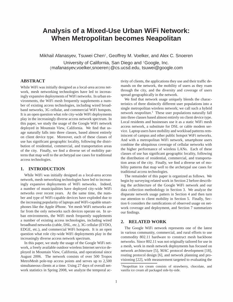
Figure 1: The Google WiFi coverage map.

prohibitions of SPAM, hacking, and other inappropriate ac-tivities, Google does not limit the types of traffic that canbe transmitted over the network,2 however it does rate limitindividual clients to 1 Mb/sec.

3.1 Network structureThe network consists of over 500 Tropos MetroMesh

pole-top access points. Each Tropos node has a distinctidentifier and a well-known geographic location; Figure 1shows the approximate location of the Tropos nodes. EachTropos node serves as an access point (AP) for client de-vices, as well as a relay node in a wide-area backhaul meshthat provides connectivity to the wired gateways. The topol-ogy of the Tropos mesh network is constructed dynamicallythrough a proprietary Tropos routing algorithm. A puremesh network of this scale exhibits significant traffic con-gestion at nodes close to the gateway router, however. Toalleviate the congestion, the Google WiFi network is hier-archically clustered around approximately 70 point-to-pointradio uplinks that serve as a fixed long-haul backbone for themesh network.

Traffic is eventually routed to one of three distinct wiredgateways spread across the city, which then forward the traf-fic to the main Google campus, where it is routed to a cen-

2The Google WiFi Terms of Service are available athttp://wifi.google.com/terms.html.

2

Field UnitsAcct-Status-Type Start/Interim-Update/StopNAS-Identifier Tropos ID stringCalling-Station-Id client MAC addressAcct-Session-Time secondsTropos-Layer2-Input-Octets (TLIO) bytesTropos-Layer2-Output-Octets (TLOO) bytesTropos-Layer2-Input-Frames (TLIF) framesTropos-Layer2-Output-Frames (TLOF) framesAcct-Input-Octets (AIO) bytesAcct-Output-Octets (AOO) bytesAcct-Input-Packets (AIP) packetsAcct-Output-Packets (AOP) packets

Table 1: Partial contents of a RADIUS log record.

tralized authorization and authentication gateway. Googleprovides single sign-on authentication and authorizationser-vice, but, at the link layer, 802.11 client devices continueas-sociate with each Tropos AP individually. All Tropos nodessupport the RADIUS accounting standard [14] and provideperiodic updates of client activity to the central server.

3.1.1 Access devices

To extend the network coverage indoors, Google recom-mends the use of WiFimodems, or bridges, which are typ-ically outfitted with more capable antennas than a standard802.11 client. WiFi modems often provide a wired Ether-net connection or serve as an in-home wireless AP, allow-ing the connection of multiple physical machines. WhileGoogle does not manufacture or sell WiFi modems, it hasrecommended two particular WiFi modems to users of theMountain View network. In particular, Google suggests thePeplink Surf and the Ruckus MetroFlex. Additionally, incertain portions of the city, Google has deployed MerakiMini mesh repeaters to extend the reach of the Tropos mesh.

3.2 Data collectionIn this study, we analyze a trace of 27 days of accounting

information collected by the central Google WiFi RADIUSserver during the Spring of 2008. Periodic updates are gen-erated by all Tropos nodes for each associated client everyfifteen minutes. Tropos nodes issue additional updates whenclients first associate or disassociate (either explicitly—which is rare—or through a 15-minute timeout). Table 1shows the portion of the RADIUS log records that we usefor our study. For the purposes of this paper, we focus al-most exclusively on layer-three information: we do not con-sider the link layer behavior of the network. (Although wedo make occasional use of layer-two accounting informationas described below.)

Additionally, to facilitate our study the types of applica-tion traffic in the network (Section 4.2.2), we obtained fivedays worth of packet-header traces collected at the centralInternet gateway of the Google WiFi network. The headertrace contains only the first packets of each flow for thefirst fifteen minutes of each hour. Because the trace wascollected at the gateway—as opposed to inside the wireless

mesh itself—we do not observe layer-two protocol trafficsuch as ARP, nor many DHCP requests which are handledby by the Tropos nodes themselves.

3.2.1 Data correction

During the course of our analysis, we discovered severalbugs in the Tropos accounting mechanism. In particular, anumber of fields are susceptible to roll-over, but such eventsare easily detectable. More significantly, the Acct-Output-Octets (AOO) field is occasionally corrupt, leading to spu-rious traffic reports for roughly 30% of all client sessions.Tropos confirms the bug, and informs us that the latest ver-sion of the Tropos software fixes it. Unfortunately, our traceswere collected before the software update was applied.

Luckily, the layer-two traffic information reported by theTropos nodes appears accurate, so we are able to both detectand correct for corrupt layer-three traffic information. Wedetect invalid log records by comparing the number of layer-two output octets (TLOO) to the layer-three count (AOO);there should always be more layer-two octets than layer-three due to link-layer headers and retransmissions. If wediscover instances where the layer-three value is larger thanlayer two, we deem the layer-three information corrupt andestimate it using layer-two information:

AOO =

AOO if AOO ≥ TLOO,

TLOO · (AOP/TLOF )

− (32 · AOP )otherwise.

In other words, we scale the layer-two octet field based uponthe ratio of layer-two frames to layer-three packets to ac-count for link-layer loss, and subtract off 32 bytes per packetfor link-layer headers.

3.2.2 Client identification

To preserve user privacy, we make no attempt to correlateindividual users with their identity through the Google au-thentication service. Instead, we focus entirely on the clientaccess device and use MAC addresses to identify users.Obviously, this approximation is not without its pitfalls—we will incorrectly classify shared devices as being oneuser, and are unable to correlate an individual user’s activityacross devices. While we speculate that a number of usersmay access the Google WiFi network with multiple distinctdevices (a laptop and smartphone, for example), we considerthis a small concession in the name of privacy.

We have aggregated clients into groups based upon theclass of device they use to access the network. We clas-sify devices based upon their manufacturer, which we de-termine based upon their MAC addresses. In particular, weuse the first three octets, commonly known as the Organiza-tionally Unique Identifier (OUI). Because many companiesmanufacture devices using different OUIs, we have manu-ally grouped OUIs from similar organizations (e.g., “Intel”and “Intel Corp.”) into larger aggregates. Table 2 showssome of the most popular OUI aggregates in our trace.

3

Class Manufacturers CountSmartphone Apple 15,450(45%) Nokia 138

Research in Motion (RIM) 107Modem Ruckus 525(3%) PepLink 297

Ambit 224Hotspot Intel 9,825(52%) Hon Hai 1,931

Gemtek 1,735Askey Computer Corp. 667Asus 385

Table 2: A selection of manufacturers in the trace anddistinct client devices seen, grouped by device class. Thefraction of total devices in each class is in parentheses.

Apple bears particular note. While we have attempted todetermine which OUIs are used for iPhones as opposed toother Apple devices (PowerBooks, MacBooks, iPod Touch,etc.), we have observed several OUIs that are in use by bothlaptops and iPhones. Hence, accurately de-aliasing theseOUI blocks would require tedious manual verification. Forthe purposes of this paper we have lumped all Apple devicestogether, and consider them all to be iPhones. Somewhatsurprisingly, this appears to be a reasonable approximation.In particular, we estimate that 88% of all Apple devices inour trace are iPhones.

In order to estimate the population of iPhone devices, weleverage the fact that Apple products periodically check forsoftware updates by polling a central server,wu.apple.com. iPhones in particular, however, polliphone-wu.apple.com, which is a CNAME forwu.apple.com.Hence, if one considers the DNS responses destined to aniPhone device polling for software updates, it will receivere-sponses corresponding to bothiphone-wu.apple.comandwu.apple.com (either because the DNS server proac-tively sent thewu.apple.com A record, or the client sub-sequently requested it). Other Apple devices, on the otherhand, will only receive an A record forwu.apple.com.We compare the total number of DNS responses destinedto clients with Apple OUIs foriphone-wu.apple.comto those forwu.apple.com present in our packet headertraces, and determine that the Gateway sees 1.13 times asmany responses forwu.apple.com. We therefore thatconclude 88% of thewu.apple.com responses actuallyresulted from queries foriphone-wu.apple.com.

iPhones constitute the vast majority of all devices we haveclassified into thesmartphonegroup, although we see sev-eral other manufacturers, including Research in Motion—makers of the Blackberry family of devices—and Nokia inthe trace. As discussed previously, Ruckus and PepLink aretwo brands of WiFi modems that Google recommended foruse in their network. Moreover, neither company appears tomanufacture other classes of WiFi devices in any large num-ber. Hence, for the remainder of the paper we have com-bined Ruckus and PepLink OUIs into a larger class that we

0

500

1000

1500

2000

2500

0 4 8 12 16 20 0

10

20

30

40

50

60

70

80

Act

ive

clie

nts

Ave

rage

act

ive

time

per

hour

(se

c)

Hour of day

Clients (weekday)Active time (weekday)

Clients (weekend)Active time (weekend)

Figure 3: Average daily use of the Google WiFi network.

term modem. (We also include Ambit, whose only WiFi-capable devices appear to be cable modems.) Finally, forlack of a better term, we classify the remaining devices ashotspotusers. While it is extremely likely that some por-tion of these devices are mis-classified (i.e., some modemand smartphone devices are likely lumped in with hotspotdevices) the general trends displayed by the hotspot usersare dominated by Intel, Hon Hai, and Gemtek, manufac-tures well known to produce a significant fraction of the in-tegrated laptop WiFi chip-sets. (Notably, Hon Hai manufac-tures WiFi chip-sets used in the Thinkpad line of laptops.)

4. USAGEIn this section we analyze when various classes of clients

are active in the Google WiFi network, and then characterizethe application workload these clients place on the network.

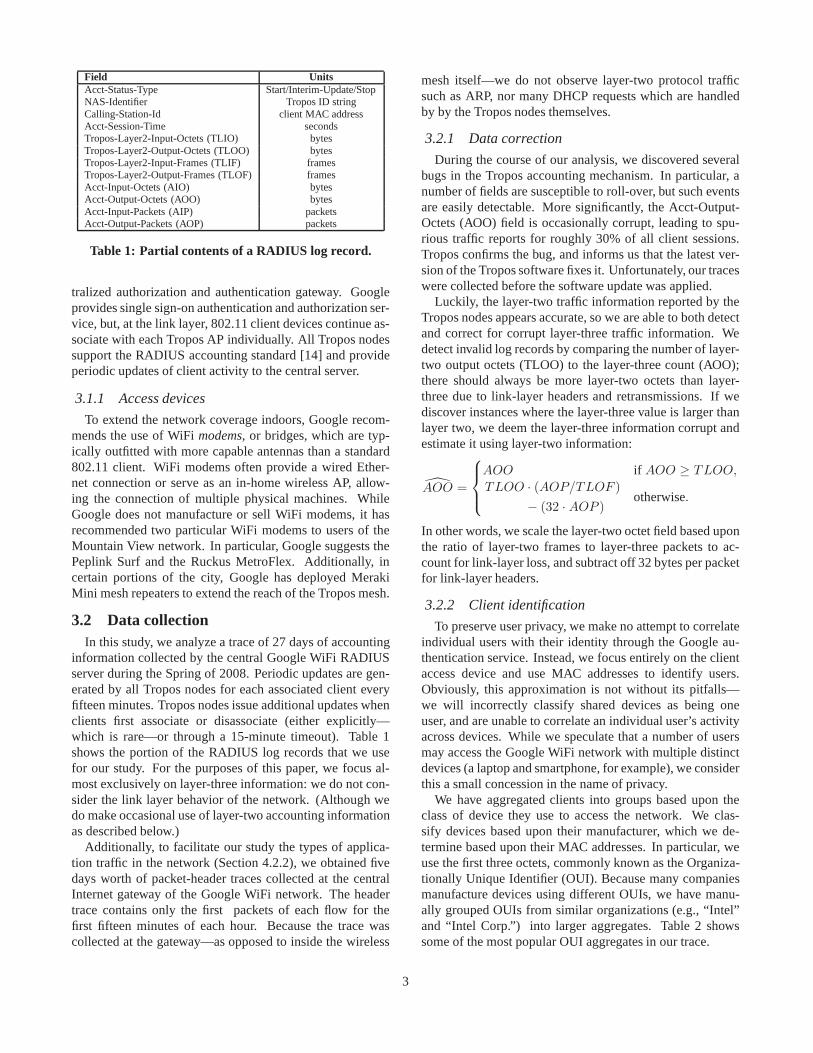
4.1 ActivityWe begin by looking at overall aggregate network activ-

ity. Figure 2 shows the number of active clients using thenetwork (lefty-axis) and their average activity time (righty-axis) per fifteen-minute interval for the entire trace. Inour analyses, we consider a client to beactive for a fifteenminute reporting interval if it sends at least one packet persecond during the interval. If a client sends fewer pack-ets, we deem it to be active for a prorated portion of theinterval—i.e., a client that sends at least 54,000 packets isdeemed active for the entire interval, while a client that sends18,000 packets is said to be active for 5 of the 15 minutes.We choose this metric in an attempt to reduce the contribu-tion of devices that are simply on but likely not being used,as such devices still tend to engage in a moderate rate ofchatter [2]. We calculate activity time as the average numberof seconds each client was active during the hour.

The results show that the Google WiFi network has a sub-stantial daily user population, peaking around 2,500 simulta-neous users in any 15-minute interval. The curves also show

4

0

500

1000

1500

2000

2500

7 14 21 0

10

20

30

40

50

60

70

80A

ctiv

e cl

ient

s

Ave

rage

act

ive

time

per

hour

(se

c)

Day

ClientsActive time

Figure 2: Usage of the Google WiFi network for the duration ofthe trace, measured in 15-minute intervals.

the typical daily variation seen in network client traces, withpeaks in both users and activity during the day roughly twicethe troughs early in the morning. Weekend use is lower thanon weekdays, with roughly 15% fewer users during peaktimes on the weekends. When users are connected, theyare active for only a small fraction of time. On an hourlybasis, users are active only between 40–80 seconds (1–2%)on average.

Figure 3 shows the daily variation of aggregate networkbehavior in more detail. The figure has four curves, twoshowing the number of clients (lefty-axis) and two show-ing average hourly client activity (righty-axis) on a typicalweekday and weekend day. At the scale of a single day, vari-ations over time in the number of clients and their activitybecome much more apparent. For example, there are mul-tiple distinct peaks in clients on the weekday during morn-ing rush hour (9 am), lunch time (12:30 pm), and the endof evening rush hour ( 6pm); weekends, however, are muchsmoother. Further, the largest peaks for the number of clientsand activity are offset by four hours. The number of clientspeaks at 6 pm at the end of rush hour, but activity peaks at10 pm late in the evening. This behavior is due to a combi-nation of the kinds of clients who are using the network andhow they use it.

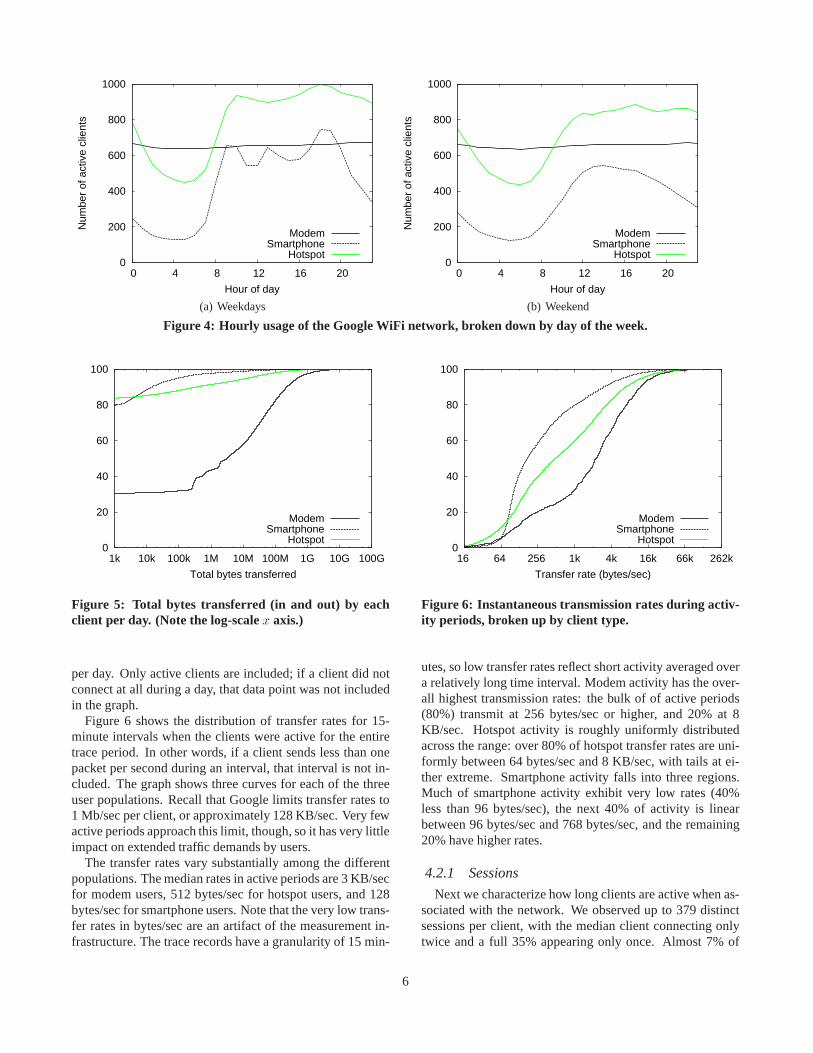
Figure 4(a) similarly shows the daily variation of clientusage on weekdays as in Figure 3, but separates clients bythe type of device they use to access the network. Thegraph shows three curves corresponding to the number ofactive modem, smartphone, and hotspot clients each hour.Separated by device type, we see that the different types ofclients have dramatically different usage profiles. The num-ber of modem clients is constant throughout the day. Thisusage suggests homes and businesses with potentially sev-eral computers powered on all day, with “chatty” operatingsystems and applications providing sufficient network trafficto keep the wireless access devices constantly active (analy-ses of network traffic in Section 4.2 shows that these users dohave substantial variation in traffic over time). Hotspot users

show more typical diurnal activity, with peak usage in lateafternoon twice the trough early in the morning. Hotspotuser activity is also high for more than half the day, from9am until 11pm at night.

Smartphone users show the most interesting variation overtime. The curve shows three distinct peaks during the day (9am, 1 pm, and 6 pm), suggesting that smartphone usage ishighly correlated with commute and travel times and thatthe devices are active while users are mobile (Section 5 ex-plores mobility behavior further). Further, smartphone us-age is much more heavily concentrated during the day. Peakclient usage at 6 pm is four times the trough at 5 am inthe morning. There are a number of possible explanationsfor this behavior. One is that the majority of smartphoneusers are commuters, and therefore are only within range ofthe network during the day. Another is that, although theymay make voice calls, users do not access WiFi during theevening, perhaps preferring to access the Internet with lap-tops or desktops when at home. The period of high activityis slightly shorter than hotspot users (9 am to 8 pm).

Figure 4(b) similarly shows the number of active clientsby device type as Figure 3, but for a typical day on the week-end. Comparing weekdays with the weekend, we see littledifference for modem and hotspot users. Modem users re-main constant, and, although there are fewer hotspots usersduring the highly active period than on the weekday, theperiod of high activity remains similar. Smartphone users,however, again exhibit the most notable differences. Smart-phone peak usage no longer correlates with commute times,peaking at midday (1pm) and diminishing steadily both be-fore and after.

4.2 TrafficThe results above show how many and when clients are

active. Next we characterize the amount of traffic activeclients generate.

Figure 5 plots the CDF of total amount of data transferred(the sum of upload and download) by clients of each class

5

0

200

400

600

800

1000

0 4 8 12 16 20

Num

ber

of a

ctiv

e cl

ient

s

Hour of day

ModemSmartphone

Hotspot

(a) Weekdays

0

200

400

600

800

1000

0 4 8 12 16 20

Num

ber

of a

ctiv

e cl

ient

s

Hour of day

ModemSmartphone

Hotspot

(b) Weekend

Figure 4: Hourly usage of the Google WiFi network, broken down by day of the week.

0

20

40

60

80

100

1k 10k 100k 1M 10M 100M 1G 10G 100G

Total bytes transferred

ModemSmartphone

Hotspot

Figure 5: Total bytes transferred (in and out) by eachclient per day. (Note the log-scalex axis.)

per day. Only active clients are included; if a client did notconnect at all during a day, that data point was not includedin the graph.

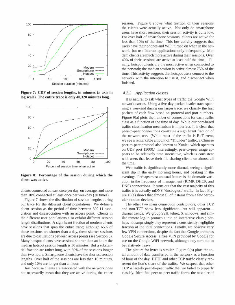
Figure 6 shows the distribution of transfer rates for 15-minute intervals when the clients were active for the entiretrace period. In other words, if a client sends less than onepacket per second during an interval, that interval is not in-cluded. The graph shows three curves for each of the threeuser populations. Recall that Google limits transfer ratesto1 Mb/sec per client, or approximately 128 KB/sec. Very fewactive periods approach this limit, though, so it has very littleimpact on extended traffic demands by users.

The transfer rates vary substantially among the differentpopulations. The median rates in active periods are 3 KB/secfor modem users, 512 bytes/sec for hotspot users, and 128bytes/sec for smartphone users. Note that the very low trans-fer rates in bytes/sec are an artifact of the measurement in-frastructure. The trace records have a granularity of 15 min-

0

20

40

60

80

100

16 64 256 1k 4k 16k 66k 262k

Transfer rate (bytes/sec)

ModemSmartphone

Hotspot

Figure 6: Instantaneous transmission rates during activ-ity periods, broken up by client type.

utes, so low transfer rates reflect short activity averaged overa relatively long time interval. Modem activity has the over-all highest transmission rates: the bulk of of active periods(80%) transmit at 256 bytes/sec or higher, and 20% at 8KB/sec. Hotspot activity is roughly uniformly distributedacross the range: over 80% of hotspot transfer rates are uni-formly between 64 bytes/sec and 8 KB/sec, with tails at ei-ther extreme. Smartphone activity falls into three regions.Much of smartphone activity exhibit very low rates (40%less than 96 bytes/sec), the next 40% of activity is linearbetween 96 bytes/sec and 768 bytes/sec, and the remaining20% have higher rates.

4.2.1 Sessions

Next we characterize how long clients are active when as-sociated with the network. We observed up to 379 distinctsessions per client, with the median client connecting onlytwice and a full 35% appearing only once. Almost 7% of

6

0

20

40

60

80

100

1 10 100 1000 10000

Session duration (minutes)

ModemSmartphone

Hotspot

Figure 7: CDF of session lengths, in minutes (x axis inlog scale). The entire trace is only 40,320 minutes long.

0

20

40

60

80

100

0 20 40 60 80 100

Percent of session time when active

ModemSmartphone

Hotspot

Figure 8: Percentage of the session during which theclient was active.

clients connected at least once per day, on average, and morethan 10% connected at least once per weekday (20 times).

Figure 7 shows the distribution of session lengths duringour trace for the different client populations. We define aclient session as the period of time between 802.11 asso-ciation and disassociation with an access point. Clients inthe different user populations also exhibit different sessionlength distributions. A significant fraction of modem clientshave sessions that span the entire trace; although 65% ofthose sessions are shorter than a day, these shorter sessionsare due to oscillations between access points (see Section 5).Many hotspot clients have sessions shorter than an hour: themedian hotspot session length is 30 minutes. But a substan-tial fraction are rather long, with 30% of the sessions longerthan two hours. Smartphone clients have the shortest sessionlengths. Over half of the sessions are less than 10 minutes,and only 10% are longer than an hour.

Just because clients are associated with the network doesnot necessarily mean that they are active during the entire

session. Figure 8 shows what fraction of their sessionsthe clients were actually active. Not only do smartphoneusers have short sessions, their session activity is quite low.For over half of smartphone sessions, clients are active forless than 10% of the time. This low activity suggests thatusers have their phones and WiFi turned on when in the net-work, but use Internet applications only infrequently. Mo-dem clients are much more active during their sessions. Over40% of their sessions are active at least half the time. Fi-nally, hotspot clients are the most active when connected tothe network; the median session is active almost 75% of thetime. This activity suggests that hotspot users connect to thenetwork with the intention to use it, and disconnect whenfinished.

4.2.2 Application classes

It is natural to ask what types of traffic the Google WiFinetwork carries. Using a five-day packet header trace span-ning a weekend during our larger trace, we classify the firstpackets of each flow based on protocol and port numbers.Figure 9(a) plots the number of connections for each trafficclass as a function of the time of day. While our port-basedtraffic classification mechanism is imperfect, it is clear thatpeer-to-peer connections constitute a significant fraction ofthe network use. (While most of the traffic is BitTorrent,we see a remarkable amount of “Thunder” traffic, a Chinesepeer-to-peer protocol also known as Xunlei, which operateson UDP port 15000.) Interestingly, peer-to-peer usage ap-pears to be relatively time insensitive, which is consistentwith users that leave their file sharing clients on almost allthe time.

Web traffic is significantly more diurnal, seeing a signif-icant dip in the early morning hours, and peaking in theevenings. Perhaps most unusual feature is the dramatic vari-ation in the frequency of management (ICMP, DHCP, andDNS) connections. It turns out that the vast majority of thistraffic is is actually mDNS “dnsbugtest” traffic. In fact, Fig-ure 10(a) shows that almost all of it stems from a few partic-ular modem devices.

The other two main connection contributors, other TCPand non-TCP show less significant—but still apparent—diurnal trends. We group SSH, telnet, X windows, and sim-ilar remote log-in protocols into an interactive class ; per-haps not surprisingly they represent a consistently negligiblefraction of the total connections. Finally, we observe veryfew VPN connections, despite the fact that Google promotesGoogle Secure Access, a free VPN provided by Google foruse on the Google WiFI network, although they turn out tobe relatively heavy.

The picture for bytes is similar. Figure 9(b) plots the to-tal amount of data transferred in the network as a functionof hour of the day. HTTP and other TCP traffic clearly rep-resent the lion’s share of the traffic. We suspect that otherTCP is largely peer-to-peer traffic that we failed to properlyclassify. Identified peer-to-peer traffic forms the next tier of

7

0

100000

200000

300000

400000

500000

0 4 8 12 16 20

Num

ber

of c

onne

ctio

ns

Hour of day

P2PMgmt

Non-TCPHTTP

Other TCPVPN

Interactive

(a) Number of connections

1

10

100

1000

10000

100000

0 4 8 12 16 20

Tot

al tr

ansf

er (

MB

)

Hour of day

HTTPOther TCP

P2PNon-TCP

VPNInteractive

Mgmt

(b) Bytes transferred

Figure 9: Hourly usage of the network per application class.

usage, along with non-TCP traffic which we suspect repre-sents VoIP and other multimedia transfers. The log-scaleyaxis provides a better view on the interactive and VPN traf-fic, which shows a subtle diurnal trend. Finally, we see thatmanagement flows, while frequent, constitute a very smallfraction of the total traffic in terms of total bytes transferred.

Figure 10 breaks down each of the two preceding graphsby client type. To do so, we build a mapping between theclient MAC addresses and assigned IP addresses in the RA-DIUS logs, and then classify the traffic logs by IP address.Not surprisingly, the three device types show markedly dif-ferent application usage. Smartphones, in particular, gen-erate very few connections, and almost all their bytes areWeb or other TCP applications. We surmise that the bulkof the other traffic is made up by streaming media (e.g.,UPnP-based iPhone video players) and VoIP traffic, but fur-ther analysis is required.

The distinctions between modem and hotspot users are farmore subtle. It is worth noting however, that there are an or-der of magnitude more hotspot users than modem users, yetthe modem users place similar aggregate traffic usage de-mands on the network. Both modem and hotspot users showa significant amount of peer-to-peer, Web, and non-TCP traf-fic. Of note, the modem P2P users appear to receive muchhigher per-connection bandwidth than the Hotspot users,which is consistent with our observations about the instan-taneous bandwidth achieved by each client type (c.f., Fig-ure 6). Hotspot users are significantly more likely to useinteractive remote login applications than modem users, butwe have not attempted to determine why that may be.

Finally, we observe that almost all the connection vol-ume in the management class stems from modem clients—Ruckus devices in particular. While many devices in ourtrace periodically issue “dnsbugtest” mDNS requests, someRuckus devices issue thousands of queries during each 15-minute interval. The precise cause of this behavior deservesfurther investigation.

0

20

40

60

80

100

0.0625 0.25 1 4 16 64 256 1024

Number of oscillations per hour of activity

ModemSmartphone

Hotspot

Figure 11: CDF of the number of oscillations per hour (xaxis is log scale).

5. MOBILITYWe now turn to questions of client mobility; in particular,

we study how frequently, fast, and far hosts move. Becauseclients do not report their geographical location, we use thelocation of the AP to which they associate as a proxy fortheir current location. The Google WiFi network has vary-ing density, but APs are approximately 100 meters apart onaverage. While that provides an effective upper bound onthe resolution of our location data, it is possible that clientsmay associate to APs other than the physically closest onedue to variations in signal propagation.

5.1 OscillationsMoreover, signal strength is a time varying process, even

for fixed clients. To gain an appreciation for the degree offluctuation in the network, we consider the number of oscil-lations in AP associations. To do so, we record the last threedistinct APs to which a client has associated. If a new asso-

8

0

50000

100000

150000

200000

250000

300000

350000

400000

0 4 8 12 16 20

Num

ber o

f con

nect

ions

Hour of day

(a) Modem connections

0 4 8 12 16 20

Hour of day

MgmtP2P

Non-TCPHTTP

Other TCPVPN

Interactive

(b) Smartphone connections

0 4 8 12 16 20

Hour of day

(c) Hotspot connections

10

100

1000

10000

0 4 8 12 16 20

Tota

l tra

nsfe

r (M

B)

Hour of day

(d) Modem bytes

0 4 8 12 16 20

Hour of day

HTTPOther TCP

P2PNon-TCP

MgmtVPN

Interactive

(e) Smartphone bytes

0 4 8 12 16 20

Hour of day

(f) Hotspot bytes

Figure 10: Number of connections (a–c) and bytes (c–e) per hour for each device type.

ciation is to one of the previous three most recent APs, weconsider it an oscillation. Using this definition, we detectahigh frequency of oscillations in the data.

Figure 11 plots the number of oscillations per hour foreach client type. Overall, we see that 50% of clients oscil-late at least once an hour, and individual clients oscillateasfrequently as 2900 times an hour (almost once a second).The rate of oscillation varies between client types, withmodems exhibiting the lowest rate of oscillation—likelybecause they are physically fixed, and oscillate only dueto environmentally induced signal strength variation—andsmartphones the highest, although the extreme tail is heav-iest for hotspot users. To more accurately capture physicalmovement—as distinct from RF movement due to changesin signal strength—we eliminate oscillations from the asso-ciation data used in the remainder of this section.

5.2 MovementWe plot the number of distinct APs to which a client asso-

ciates during the course of our trace in Figure 12. Roughly35% of all devices associate with only one AP; this corre-sponds well to the fraction of clients that appear only oncein the trace (c.f. Section 4.2.1). As one might expect, eachclient class exhibits markedly different association behavior.Modems tend to associate with a very few number of APs—likely nearby to a single physical location. Smartphones, onthe other hand, frequently associate with a large number ofAPs; 50% of smartphones associate with at least six distinctAPs, and the most wide-ranging of 10% smartphones asso-ciate with over 32 APs. Hotspot clients, on the other hand,are significantly less mobile—the 90% percentile associateswith less than 16 APs during the four-week trace. We ob-

0

20

40

60

80

100

1 2 4 8 16 32 64 128 256

Number of distinct APs

ModemSmartphone

Hotspot

Figure 12: CDF of the number of distinct APs a clientassociates with over the course of the trace.

serve, however, that both the smartphone and hotspot pop-ulations are skewed by a significant number of clients thatappear only once in the entire trace.

If we restrict the time window to a day—as opposed to28 days as above—he distribution shifts considerably (notshown): 90% of all clients connect to at most eight APs perday on average, with only a handful of clients connecting tomore than 16 APs. A fully 90% of modems, 70% of hotspotusers, and 40% of smartphones connect to only one AP perday on average.

Next, we consider how geographically disperse these APsare. In particular, we study the distance traveled betweenconsecutive associations by a single client. Figure 13 plotsthe average distance in meters between non-oscillatory client

9

0

20

40

60

80

100

100 1000 10000

Distance between APs (meters)

ModemSmartphone

Hotspot

Figure 13: CDF of the average distance between consec-utive client associations.

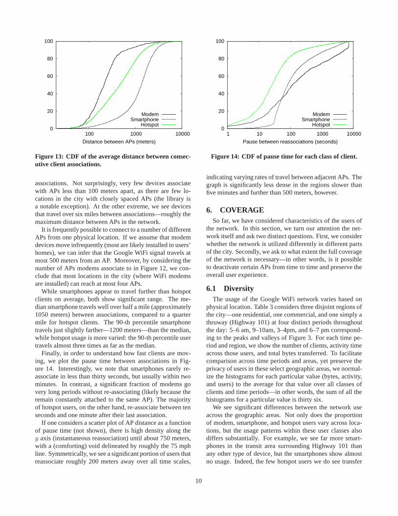
associations. Not surprisingly, very few devices associatewith APs less than 100 meters apart, as there are few lo-cations in the city with closely spaced APs (the library isa notable exception). At the other extreme, we see devicesthat travel over six miles between associations—roughly themaximum distance between APs in the network.

It is frequently possible to connect to a number of differentAPs from one physical location. If we assume that modemdevices move infrequently (most are likely installed in users’homes), we can infer that the Google WiFi signal travels atmost 500 meters from an AP. Moreover, by considering thenumber of APs modems associate to in Figure 12, we con-clude that most locations in the city (where WiFi modemsare installed) can reach at most four APs.

While smartphones appear to travel further than hotspotclients on average, both show significant range. The me-dian smartphone travels well over half a mile (approximately1050 meters) between associations, compared to a quartermile for hotspot clients. The 90-th percentile smartphonetravels just slightly farther—1200 meters—than the median,while hotspot usage is more varied: the 90-th percentile usertravels almost three times as far as the median.

Finally, in order to understand how fast clients are mov-ing, we plot the pause time between associations in Fig-ure 14. Interestingly, we note that smartphones rarely re-associate in less than thirty seconds, but usually within twominutes. In contrast, a significant fraction of modems govery long periods without re-associating (likely because theremain constantly attached to the same AP). The majorityof hotspot users, on the other hand, re-associate between tenseconds and one minute after their last association.

If one considers a scatter plot of AP distance as a functionof pause time (not shown), there is high density along they axis (instantaneous reassociation) until about 750 meters,with a (comforting) void delineated by roughly the 75 mphline. Symmetrically, we see a significant portion of users thatreassociate roughly 200 meters away over all time scales,

0

20

40

60

80

100

1 10 100 1000 10000

Pause between reassociations (seconds)

ModemSmartphone

Hotspot

Figure 14: CDF of pause time for each class of client.

indicating varying rates of travel between adjacent APs. Thegraph is significantly less dense in the regions slower thanfive minutes and further than 500 meters, however.

6. COVERAGESo far, we have considered characteristics of the users of

the network. In this section, we turn our attention the net-work itself and ask two distinct questions. First, we considerwhether the network is utilized differently in different partsof the city. Secondly, we ask to what extent the full coverageof the network is necessary—in other words, is it possibleto deactivate certain APs from time to time and preserve theoverall user experience.

6.1 DiversityThe usage of the Google WiFi network varies based on

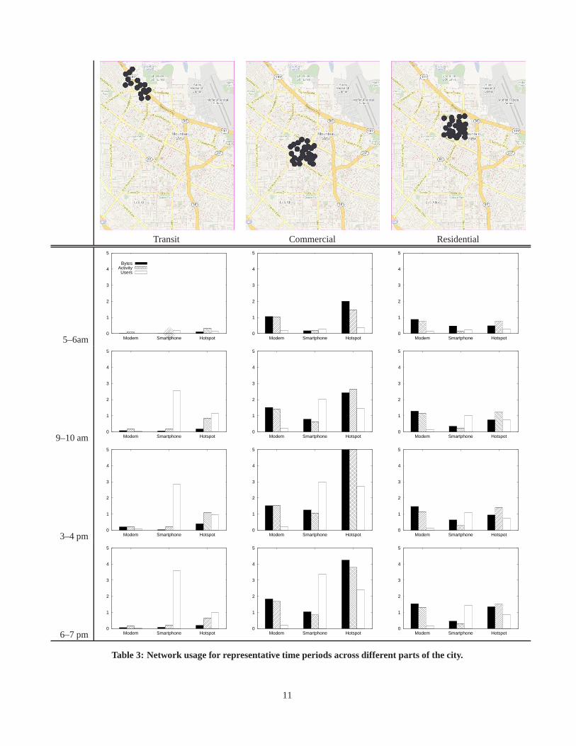
physical location. Table 3 considers three disjoint regions ofthe city—one residential, one commercial, and one simply athruway (Highway 101) at four distinct periods throughoutthe day: 5–6 am, 9–10am, 3–4pm, and 6–7 pm correspond-ing to the peaks and valleys of Figure 3. For each time pe-riod and region, we show the number of clients, activity timeacross those users, and total bytes transferred. To facilitatecomparison across time periods and areas, yet preserve theprivacy of users in these select geographic areas, we normal-ize the histograms for each particular value (bytes, activity,and users) to the average for that value over all classes ofclients and time periods—in other words, the sum of all thehistograms for a particular value is thirty six.

We see significant differences between the network useacross the geographic areas. Not only does the proportionof modem, smartphone, and hotspot users vary across loca-tions, but the usage patterns within these user classes alsodiffers substantially. For example, we see far more smart-phones in the transit area surrounding Highway 101 thanany other type of device, but the smartphones show almostno usage. Indeed, the few hotspot users we do see transfer

10

Transit Commercial Residential

5–6am 0

1

2

3

4

5

Modem Smartphone Hotspot

BytesActivityUsers

0

1

2

3

4

5

Modem Smartphone Hotspot 0

1

2

3

4

5

Modem Smartphone Hotspot

9–10 am 0

1

2

3

4

5

Modem Smartphone Hotspot 0

1

2

3

4

5

Modem Smartphone Hotspot 0

1

2

3

4

5

Modem Smartphone Hotspot

3–4 pm 0

1

2

3

4

5

Modem Smartphone Hotspot 0

1

2

3

4

5

Modem Smartphone Hotspot 0

1

2

3

4

5

Modem Smartphone Hotspot

6–7 pm 0

1

2

3

4

5

Modem Smartphone Hotspot 0

1

2

3

4

5

Modem Smartphone Hotspot 0

1

2

3

4

5

Modem Smartphone Hotspot

Table 3: Network usage for representative time periods across different parts of the city.

11

0

10

20

30

40

50

60

70

80

90

100

0 100 200 300 400 500

Fra

ctio

n of

act

ivity

tim

e re

mai

ning

Number of access points removed

Figure 15: Effect of removing Tropos access points ontotal network activity time.

more data cumulatively than the smartphones. In contrast,smartphones are far less prevalent in the residential area,ap-pearing in similar numbers to hotspot users. However, thosewe do observe are substantially more active than those in thetransit area. Not surprisingly, modem users represent a sig-nificant fraction of the residential usage, at least in termsoftraffic and activity if not in total number. Moreover, theirusage appears less time dependent than the other devices.

The commercial area is the most active, with significantusage across all three classes of clients. Modem activityis similar to that in residential areas, but the absolute num-ber of both smartphones and hotspot users is significantlyhigher. Mobile (i.e., smartphone and hotspot) usage peaks inthe commercial area in the middle of the afternoon (hotspotusage is off scale, with a normalized byte count of 6.2 anduser count of 5.4), yet remains strong across all periods, un-like the other two, which show far less usage in the earlymorning hours. Unsurprisingly, the number of clients in thetransit area peaks during rush hours, while residential usageis highest during the evening (not shown).

6.2 ConcentrationFor a metropolitan network covering an entire city, an in-

teresting deployment question is to what extent the full setofnodes in the network are actively being used. As a final ex-periment, we calculated the total activity time for each poletop Tropos node. We then sorted the nodes in increasing ac-tivity time, with the least active node first. Starting with allof the nodes, we then successively removed nodes in sortedorder. At each step, we calculated the fraction of activitytime contributed by all of the nodes together — the first stepcorresponds to the activity of all of the nodes, the second toall nodes minus the least active node, etc.

Figure 15 shows the distribution of activity time for thisexperiment. Thex-axis shows the number of access pointsremoved (in sorted order of increasing activity time). They-axis shows the fraction of all activity time a given set of

nodes contribute. Somewhat surprisingly, we do not find aheavy tail to the curve, indicating that all nodes are relativelyactive and contribute to useful network coverage throughoutMountain View.

7. CONCLUSIONIn this paper, we study the usage of the Google WiFi net-

work, a freely available outdoor wireless Internet servicedeployed in Mountain View, California. We find that theaggregate usage of the Google WiFi network is composedof three distinct user populations, characterized by distincttraffic, mobility, and usage patterns that are characteristic oftraditional wireline, wide-area, and localized wireless accessnetworks. Modem users are static and always connected, andplace the highest demand on the network. Hotspot users areconcentrated in commercial and public areas, and have mod-erate mobility. Smartphone users are surprisingly numerous,have peak activity strongly correlated with commute timesand are concentrated along travel corridors, yet place verylow demands on the network.

8. REFERENCES

[1] D. Aguayo, J. Bicket, S. Biswas, G. Judd, and R. Morris. Link-levelMeasurements from an 802.11b Mesh Network. InProceedings ofACM SIGCOMM, 2004.

[2] M. Allman, K. Christensen, B. Nordman, and V. Paxson. Enabling anenergy-efficient future internet. InProceedings of HotNets, Nov.2007.

[3] A. Balachandran, G. M. Voelker, P. Bahl, and P. V. Rangan.Characterizing User Behavior and Network Performance in a PublicWireless LAN. InProceedings of ACM SIGMETRICS, June 2002.

[4] M. Balazinska and P. Castro. Characterizing Mobility and NetworkUsage in a Corporate Wireless Local-Area Network. InProceedingsof USENIX MobiSys, 2003.

[5] J. Bicket, D. Aguayo, S. Biswas, and R. Morris. Architecture andEvaluation of an Unplanned 802.11b Mesh Network . InProceedingsof Mobicom, August 2005.

[6] S. Biswas and R. Morris. Opportunistic Routing in Multi-HopWireless Networks. InProceedings of SIGCOMM, August 2005.

[7] Y.-C. Cheng, M. Afanasyev, P. Verkaik, P. Benko, J. Chiang, A. C.Snoeren, S. Savage, and G. M. Voelker. Automating cross-layerdiagnosis of enterprise wireless networks. InProceedings of the ACMSIGCOMM Conference, Kyoto, Japan, Aug. 2007.

[8] Y.-C. Cheng, J. Bellardo, P. Benko, A. C. Snoeren, G. M. Voelker,and S. Savage. Jigsaw: Solving the puzzle of enterprise 802.11analysis. InProceedings of the ACM SIGCOMM Conference, pages39–50, Pisa, Italy, Sept. 2006.

[9] T. Henderson, D. Kotz, and I. Abyzov. The Changing Usage of aMature Campus-wide Wireless Network. InProceedings of ACMMobicom, Sept. 2004.

[10] F. Hernandez-Campos and M. Papadopouli. A ComparativeMeasurement Study of the Workload of Wireless Access PointsinCampus Networks. InProceedings of IEEE PIMRC, 2005.

[11] A. P. Jardosh, K. N. Ramachandran, K. C. Almeroth, and E.M.Belding-Royer. Understanding Congestion in IEEE 802.11b WirelessNetworks. InProceedings of ACM IMC, Oct. 2005.

[12] A. P. Jardosh, K. N. Ramachandran, K. C. Almeroth, and E.M.Belding-Royer. Understanding Link-Layer Behavior in HighlyCongested IEEE 802.11b Wireless Networks. InProceedings ofACM E-WIND, Aug. 2005.

[13] D. Kotz and K. Essien. Analysis of a Campus-wide WirelessNetwork. InProceedings of ACM Mobicom, Sept. 2002.

[14] C. R. Livingston. Radius accounting. RFC 2866, IETF, June 2000.

12

[15] R. Mahajan, M. Rodrig, D. Wetherall, and J. Zahorjan. Analyzing theMAC-level Behavior of Wireless Networks in the Wild. InProceedings of ACM SIGCOMM, Sept. 2006.

[16] M. McNett and G. M. Voelker. Access and Mobility of Wireless PDAUsers.Mobile Computing and Communications Review, 9(2), 2005.

[17] K. N. Ramachandran, E. M. Belding-Royer, and K. C. Almeroth.DAMON: A Distributed Architecture for Monitoring Multi-hopMobile Networks. InProceedings of IEEE SECON, 2004.

[18] B. Raman and K. Chebrolu. Design and Evaluation of a new MACProtocol for Long-Distance 802.11 Mesh Networks. InProceedingsof the 11th Annual International Conference on Mobile Computingand Networking (MobiCom’05), August 2005.

[19] B. Raman and K. Chebrolu. Experiences in using WiFi for RuralInternet in India.IEEE Communications Magazine, Special Issue onNew Directions In Networking Technologies In Emerging Economies,45(1):104–110, January 2007.

[20] M. Rodrig, C. Reis, R. Mahajan, D. Wetherall, and J. Zahorjan.Measurement-based Characterization of 802.11 in a HotspotSetting.In Proceedings of ACM E-WIND, 2005.

[21] D. Schwab and R. Bunt. Characterising the Use of a CampusWireless Network. InProceedings of IEEE Infocom, 2004.

[22] S. Sen and B. Raman. Long Distance Wireless Mesh NetworkPlanning: Problem Formulation and Solution. InProceedings of the16th Annual International World Wide Web Conference (WWW2007).

[23] D. Tang and M. Baker. Analysis of a Local-Area Wireless Network.In Proceedings of ACM Mobicom, 2000.

[24] D. Tang and M. Baker. Analysis of a metropolitan-area wirelessnetwork.Wireless Networks, 8:107–120, 2002.

[25] S. Thajchayapong and J. M. Peha. Mobility Patterns in MicrocellularWireless Networks. InProceedings of IEEE WirelessCommunications and Networking Conference (WCNC), March 2003.

13