Optimisation d'un magnétomètre à haute sensibilité à base de ...
HAL Id: tel-01143779https://tel.archives-ouvertes.fr/tel-01143779
Submitted on 20 Apr 2015
HAL is a multi-disciplinary open accessarchive for the deposit and dissemination of sci-entific research documents, whether they are pub-lished or not. The documents may come fromteaching and research institutions in France orabroad, or from public or private research centers.
L’archive ouverte pluridisciplinaire HAL, estdestinée au dépôt et à la diffusion de documentsscientifiques de niveau recherche, publiés ou non,émanant des établissements d’enseignement et derecherche français ou étrangers, des laboratoirespublics ou privés.
Analyse de sensibilité en fiabilité des structuresPaul Lemaitre
To cite this version:Paul Lemaitre. Analyse de sensibilité en fiabilité des structures. Mécanique des structures[physics.class-ph]. Université de Bordeaux, 2014. Français. NNT : 2014BORD0061. tel-01143779
THÈSE PRÉSENTÉE
POUR OBTENIR LE GRADE DE
DOCTEUR DE
L’UNIVERSITÉ DE BORDEAUX
ÉCOLE DOCTORALE DE MATHÉMATIQUES ET INFORMATIQUE
SPÉCIALITÉ : Mathématiques appliquées
Par Paul Lemaître
Analyse de sensibilité en fiabilité des Structures
Directeur de thèse : M. Pierre Del Moral
Soutenue le 18 mars 2014 devant la commission d'examen composée de : M. Josselin Garnier Professeur Université Paris VII Rapporteur M. Bertrand Iooss Chercheur Senior EDF R& D Co-encadrant M. François Legland Dir. de Recherche INRIA Rennes Rapporteur M. Emmanuel Remy Chercheur Expert EDF R& D Examinateur M. Jérôme Saracco Professeur Inst. Poly. de Bordeaux xaminateur
Titre : Analyse de sensibilité en fiabilité des structures Résumé : Cette thèse porte sur l'analyse de sensibilité dans le contexte des études de fiabilité des structures. On considère un modèle numérique déterministe permettant de représenter des phénomènes physiques complexes. L'étude de fiabilité a pour objectif d'estimer la probabilité de défaillance du matériel à partir du modèle numérique et des incertitudes inhérentes aux variables d'entrée de ce modèle. Dans ce type d'étude, il est intéressant de hiérarchiser l'influence des variables d'entrée et de déterminer celles qui influencent le plus la sortie, ce qu'on appelle l'analyse de sensibilité. Ce sujet fait l'objet de nombreux travaux scientifiques mais dans des domaines d'application différents de celui de la fiabilité. Ce travail de thèse a pour but de tester la pertinence des méthodes existantes d'analyse de sensibilité et, le cas échéant, de proposer des solutions originales plus performantes. Plus précisément, une étape bibliographique sur l'analyse de sensibilité puis sur l'estimation de faibles probabilités de défaillance est proposée. Cette étape soulève le besoin de développer des techniques adaptées. Deux méthodes de hiérarchisation de sources d'incertitudes sont explorées. La première est basée sur la construction de modèle de type classifieurs binaires (forêts aléatoires). La seconde est basée sur la distance, à chaque étape d'une méthode de type subset, entre les fonctions de répartition originelle et modifiée. Une méthodologie originale plus globale, basée sur la quantification de l'impact de perturbations des lois d'entrée sur la probabilité de défaillance est ensuite explorée. Les méthodes proposées sont ensuite appliquées sur le cas industriel CWNR, qui motive cette thèse. Mots clés : Analyse de sensibilité ; Fiabilité; Incertitudes ; Expériences numériques; Perturbation des lois
Title : Reliability sensitivity analysis Abstract : This thesis' subject is sensitivity analysis in a structural reliability context. The general framework is the study of a deterministic numerical model that allows to reproduce a complex physical phenomenon. The aim of a reliability study is to estimate the failure probability of the system from the numerical model and the uncertainties of the inputs. In this context, the quantification of the impact of the uncertainty of each input parameter on the output might be of interest. This step is called sensitivity analysis. Many scientific works deal with this topic but not in the reliability scope. This thesis' aim is to test existing sensitivity analysis methods, and to propose more efficient original methods. A bibliographical step on sensitivity analysis on one hand and on the estimation of small failure probabilities on the other hand is first proposed. This step raises the need to develop appropriate techniques. Two variables ranking methods are then explored. The first one proposes to make use of binary classifiers (random forests). The second one measures the departure, at each step of a subset method, between each input original density and the density given the subset reached. A more general and original methodology reflecting the impact of the input density modification on the failure probability is then explored. The proposed methods are then applied on the CWNR case, which motivates this thesis. Keywords : Sensitivity Analysis; Reliability; Uncertainties; Computer experiments; Input perturbations

Cette thèse est une grande aventure qui ommença en dé embre 2008, à Lyngby, Danemark. A
ette époque, jeune étudiant Erasmus en quête d'un stage de 4ème année, j'ai vu arriver dans ma
boîte mail une proposition de stage en analyse d'in ertitudes au CEA de Cadara he. Un ami, que je
dénon e plus tard, m'a aidé à passer le ap du "j'ai pas le niveau" et m'a poussé à andidater. Bien
m'en a pris, ar e stage fut le début d'une fru tueuse ollaboration. C'est le moment de remer ier
toutes les personnes sans qui la thèse n'aurait tout simplement pas été possible.
Que e soit à Tunis, Cadara he, Chatou ou à Villard de Lans, Bertrand Iooss a su faire montre
d'une grande humanité et de ompéten es s ientiques très poussées sous ouvert d'une arapa e
punk. Je lui suis très re onnaissant de m'avoir transmis une bonne partie de ses onnaissan es, je
l'espère pas uniquement statistiques.
Mer i à Fabri e Gamboa pour m'avoir permis de nir ma thèse dans de bonnes onditions, je
lui suis inniment re onnaissant de m'avoir a epté omme obureau ("room servi e") pour les 5
derniers mois.
Je remer ie Pierre Del Moral d'avoir a epté de m'en adrer au titre de dire teur de thèse. De la
même façon, je sais gré à Josselin Garnier et François Le Gland d'avoir patiemment relu ette thèse
et d'avoir apporté des remarques pertinentes me permettant d'améliorer le résultat. Mer i aussi à
Jérme Sara o pour avoir a epté de faire partie du jury.
Une bonne partie de ma gratitude va à Aurélie Arnaud pour son en adrement orienté appli ations.
De la même façon, je suis parti ulièrement re onnaissant envers Emmanuel "Manu" Remy, pour
m'avoir supporté dans son ouloir à des heures que le ode du travail réprouve, pour ses onnaissan es
sur la physique des réa teurs et pour ses (très) patientes rele tures.
Ma re onnaissan e va également à Agnès Lagnoux pour m'avoir en adré lors d'un ourt mais
e a e séjour de re her he à l'UPS n 2012.
C'est l'o asion pour moi de dire la gratitude que j'ai envers Didier Larrauri pour m'avoir au-
torisé à prolonger ma thèse an de la nir dans de bonnes onditions. J'ai pu appré ier pendant
ette thèse d'être entouré de ollègues à la fois sympathiques et e a es, pointus en statistiques et
en appli atif. Mes hommages à tout MRI, T-55 et T-57 en tête. En parti ulier, je remer ie Mathieu
pour son aide sur la partie logi ielle et Mi hael pour son savoir des ar anes du al ul numérique
ainsi que Merlin pour avoir patiemment é outé mes élu ubrations, notamment sur la partie "pertur-
bation des paramètres" des DMBRSI. À mon "on le de thèse" Ni olas, j'adresse mes plus sin ères
remer iements. Mer i de m'avoir rassuré à plusieurs o asions sur l'avenir de ette thèse. Et bien
sûr, salutations sportives pour mes deux ollègues de salle de sport Popi et Fafa.
Cette thèse n'aurait pas vu le jour sans le fort support dans tous les moments di iles que j'ai
eu de la part de mes amis. En parti ulier je remer ie le trio parisien formé par Jean-Phi, Thierno et
Nessie, pour les bons moments et les autres. Des poutoux à Morgane et Diday. Il me faut également
tirer mon hapeau à l'équipe toulousaine, Dra o et Maria en tête. Je remer ie également Bébert
(il sait pourquoi). Big up à Raphaël, pour m'avoir e a ement onseillé sur tout l'interfaçage ave
l'Université de Bordeaux. Mention spé iale à Petit Paul, Agathe, Alex et Mélo pour l'anglais. Par
ailleurs, je suis redevable à eux qui prendront la peine de poser un RTT pour aller jusqu'à Bordeaux
le jour de ma soutenan e, Fly, Quentin, Jeb et tonton Vip - hop dénon é. Enn, je ne peux on lure
sans une pensée pour Mathieu.
Pour nir, mes sentiments vont vers ma famille, en parti ulier mes parents et mes deux s÷urs
qui furent pendant ette épreuve la dénition même d'indéfe tible.

Résumé étendu
Introdu tion
Analyse d'in ertitudes et expérien es numériques
On présente i i brièvement le adre général de ette thèse : l'exploitation d'un modèle numérique.
Un modèle est i i une représentation mathématique d'un phénomène physique et son traitement est
ee tué au travers d'un système de al ul.
Ce modèle possède des entrées et des sorties (ou réponses). I i, toutes es quantités seront
onsidérées s alaires mais d'autres types pourraient être envisagés, modales par exemple. En fon tion
d'un jeu de données d'entrée, le ode de al ul va produire un jeu de réponses après un ertain temps
de al ul. Le adre des odes déterministes est utilisé : un même jeu d'entrée produira toujours le
même jeu de sortie. Dans e rapport, il sera parfois fait un abus de langage en assimilant le ode au
modèle, pour des raisons de lisibilité.
Une notion essentielle est la quantité d'intérêt. Il est en eet possible que e ne soit pas une valeur
de sortie qui intéresse l'expérimentateur, mais plutt une plage de valeurs ou une quantité dénie
à partir des sorties. Il est don primordial avant toute étude de dénir quelle est la quantité d'intérêt.
L'analyse de sensibilité est dénie par Saltelli et al. [89 omme l'étude de la façon dont
l'in ertitude sur une quantité de sortie du modèle peut être attribuée aux diérentes sour es d'in ertitudes
dans les variables d'entrée.
L'analyse de sensibilité d'un modèle numérique peut servir à déterminer les variables d'entrée qui
ontribuent le plus à un ertain omportement d'une sortie, déterminer elles sans inuen e ou elles
qui vont interagir à travers le modèle. Le but peut être de omprendre le modèle, de le simplier, ou
en ore de prioriser le re ueil de données pour mieux modéliser une variable d'entrée. Une appro he
ré ente est l'appro he dite globale. L'ensemble du domaine de variation des variables d'entrée est
alors étudié. La plupart des te hniques sont développées dans une appro he indépendante du modèle
("model free"), 'est-à-dire sans émettre d'hypothèses sur le omportement du modèle omme par
exemple la linéarité ou la monotonie.
Fiabilité des stru tures
On her he à répondre au problème industriel de savoir si une stru ture ou un omposant peut résister
à des ontraintes qui lui sont appliquées. L'appro he basée sur des essais et mesures est possible,
mais peut s'avérer di ile pour des raisons de oûts ou de risques. Parfois, l'expérimentation est
impossible. Des modèles numériques sont alors utilisés omme représentation appro hée de la réalité
in luant ertains mé anismes ( omme par exemple eux de la dégradation, de la propagation des
ssures...).
An d'exploiter omplètement le modèle, les in ertitudes sur les paramètres d'entrées du ode
(essentiellement des grandeurs physiques) sont modélisées par des variables aléatoires. Le modèle
5
Résumé étendu
représente don la stru ture, dotée d'une ertaine résistan e, et l'environnement, qui engendre une
solli itation. Le al ul pour un jeu d'entrées xées permet d'obtenir un ritère de défaillan e qui
amène à une réponse binaire : la stru ture est défaillante pour es entrées ou non défaillante.
Le fait d'in lure les in ertitudes omme des variables aléatoires permet de modéliser le risque
omme une probabilité de défaillan e. Cette appro he est plus ne qu'une appro he déterministe où
les grandeurs sont xées à des valeurs nominales.
Soit X = (X1, ...Xd) le ve teur aléatoire d−dimensionnel (dont la densité fX est onnue) des
variables d'entrée (s alaires) du modèle numérique. On s'intéresse à e que la valeur s alaire Y ∈ R
renvoyée par la fon tion de défaillan e G du modèle (ou fon tion d'état-limite du modèle) soit plus
faible qu'un ertain seuil k (usuellement 0) : 'est le ritère de défaillan e. La stru ture est défaillantepour un jeu d'entrée x si y = G(x) ≤ k (où x = (x1, ..., xd) ∈ Rd
est une réalisation de X et k un
seuil usuellement xé à 0). L'ensemble de l'espa e sur lequel et évènement se produit est appelé
domaine de défaillan e Df . La surfa e dénie par x ∈ Rd, G(x) = k est dite surfa e d'état-limite.
La probabilité que l'évènement se produise est notée Pf , probabilité de défaillan e. On a :
Pf = P(G(X) ≤ k)
=
Df
fX(x)dx
=
Rd
1G(x)≤kfX(x)dx
= E[1G(X)≤k]
La omplexité des modèles et le possible grand nombre de variables d'entrée fait que, dans le as
général, on ne peut pas al uler la valeur exa te de la probabilité de défaillan e. On peut epen-
dant estimer ette quantité (qui est une espéran e mathématique) à l'aide de diverses méthodes
numériques. La base de la abilité des stru tures est de fournir une estimation de Pf et une in erti-
tude autour de ette estimation. Cette estimation permet ensuite de répondre à la question initiale
de la résistan e de la stru ture.
Obje tifs de la thèse
Le but de ette thèse est le développement de te hniques d'analyse de sensibilité quand la quantité
d'intérêt est une probabilité de dépassement de seuil ( e qui équivaut à une probabilité de défaillan e
dans le ontexte de la abilité des stru tures). Les ontraintes du ode CWNR qui a motivé le travail
de thèse doivent être prises en ompte. La probabilité de défaillan e dans le as le moins pénalisant
(7 variables) a un ordre de grandeur attendu de 10−5. Si possible, les méthodes développées doivent
être en relation ave l'estimation de Pf et doivent produire une estimation de l'erreur faite lors de
l'estimation des indi es de sensibilité et de Pf .
Organisation de la thèse
La thèse est divisée en quatre hapitres.
Le premier hapitre est une revue des stratégies existantes pour estimer des probabilités de
défaillan e et des te hniques d'analyse de sensibilité.
Le se ond hapitre est onsa ré à la dénition de mesures de sensibilité ave pour but la produ -
tion d'un lassement de variables (variable ranking).
6

Le troisième hapitre présente une méthode originale pour estimer l'importan e de ha une des
variables d'entrée sur une probabilité de défaillan e. Cette méthode se on entre sur l'impa t d'une
modi ation de densité d'entrée sur la probabilité de défaillan e produite en sortie.
Le quatrième hapitre présente une appli ation des méthodes étudiées sur le as CWNR, as réel
qui a motivé la thèse.
Méthodes de lassement de variables
Le se ond hapitre présente deux méthodes permettant de lasser les variables d'entrée en fon tion
de leur inuen e sur la sortie (binaire). De plus, es méthodes sont des sous-produits de l'estimation
de la probabilité de défaillan e Pf .
En eet la première te hnique propose de faire usage de mesures dérivées de l'ajustement de
forêts aléatoires sur un é hantillon de type Monte-Carlo. Un rappel sur les arbres binaires puis sur
les forêts aléatoires est proposé, puis l'étude de deux indi es (Gini Importan e et Mean De rease
A ura y) mesurant l'importan e des variables sur la quantité d'intérêt binaire est proposé.
La se onde te hnique mesure l'é art, à haque étape d'une méthode de type subset simulation,
entre les densités d'entrée et les densités sa hant que le sous-ensemble est atteint.
La dénition informelle est la suivante : l'indi e de sensibilité est déni pour la variable i etl'étape du subset k omme la distan e entre la fon tion de répartition (f.d.r.) empirique et la f.d.r.
théorique de la variable. Considérant M étapes de subset ave k = 1 . . .M ; et en notant :
F kn,i = Fi(x|Ak),
la f.d.r. empirique de la ième
variable sa hant que le seuil Ak a été dépassé. L'indi e proposé s'é rit
omme suit :
δSSi (Ak) = d(F kn,i, Fi),
où Fi est la f.d.r. de la ième
variable, et d est une distan e. Une variable inuente aura un grand
é art en f.d.r alors qu'une variable non-inuente aura un faible é art en f.d.r., don un faible indi e.
Des travaux sont menés sur le hoix de la distan e d en fon tion du besoin de l'analyste.
Ces deux méthodes peuvent don être vues omme des sous-produits de te hniques d'estimation
de la probabilité de défaillan e.
Méthode basée sur une perturbation des densités (DMBRSI)
Dans le troisième hapitre, de nouveaux indi es de sensibilité pour la abilité sont proposés. Cet
indi e de sensibilité est basé sur une modi ation des densités et est adapté aux probabilités de
défaillan e. Une méthode pour estimer de tels indi es est proposée.
Ces indi es reètent l'impa t d'une modi ation d'une densité d'entrée sur la probabilité de
défaillan e Pf . Ils sont indépendants de la perturbation dans le sens où l'utilisateur peut hoisir la
perturbation adaptée à son problème.
Pour des raisons de simpli ité, un s héma d'é hantillonnage Monte-Carlo lassique est onsid-
éré par la suite, bien que le pro essus d'estimation a été étendu aux méthodes subset et tirages
d'importan e. Les indi es de sensibilité peuvent être estimés en utilisant seulement le jeu de simu-
lations déjà utilisé pour estimer la probabilité de défaillan e Pf . Ce i limite le nombre d'appels au
ode de al ul, omme mentionné dans les ontraintes du as industriel CWNR.
Le hapitre est organisé de la façon suivante : en premier lieu, les indi es et leurs propriétés
théoriques sont présentées ainsi qu'une méthode d'estimation. En se ond lieu, plusieurs méthodes
7
Résumé étendu
de perturbation des densités sont présentées. Ces modi ations peuvent être lassées en deux grandes
familles : minimisation de Kullba k-Leibler et perturbation des paramètres. Le omportement des
indi es proposés est testé sur des as tests, puis les avantages et problèmes restants sont nalement
dis utés.
Le hapitre 3 est une version étendue du papier par Lemaître et oauteurs [63.
Indi e DMBRSI
Soit une entrée unidimensionnelle Xi de densité fi, on appelle Xiδ ∼ fiδ l'entrée perturbée orre-
spondante.
La probabilité de défaillan e modiée devient :
Piδ =
1G(x)<0fiδ(xi)
fi(xi)f(x)dx
où xi est la ième
omposante du ve teur x.
L'indi e DMBRSI a la forme suivante.
Dénition On dénit les indi es de sensiblité basés sur une modi ation des lois (Density Modi-
ation Based Reliability Sensitivity Indi es - DMBRSI) omme la quantité Siδ :
Siδ =
[Piδ
Pf− 1
]1Piδ≥Pf +
[1− Pf
Piδ
]1Piδ<Pf =
Piδ − Pf
Pf · 1Piδ≥Pf + Piδ · 1Piδ<Pf.
Estimation
Un estimateur PN de Pf peut être al ulé en utilisant un plan d'expérien e de N points. Par la
suite, N est onsidéré omme étant assez grand pour que le ontexte de la théorie asymptotique
s'applique. Par ailleurs, un é hantillonnage de type Monte-Carlo standard est utilisé pour simplier
les al uls. On é rit alors
PN =1
N
N∑
n=1
1G(xn)<0
où x1, · · · ,xNsont des réalisations indépendantes de X. La loi forte des grands nombres et le
théorème limite entrale (TLC) assurent que pour presque toutes les réalisations, PN −−−−→N→∞
Pf et
√N
Pf (1− Pf )(PN − Pf )
L−−−−→N→∞
N (0, 1).
Le adre Monte-Carlo permet d'estimer Piδ de façon onsistante sans nouvel appel au ode de
al ul G, grâ e à une te hnique de tirage d'importan e "inverse" (reverse importan e sampling):
PiδN =1
N
N∑
n=1
1G(xn)<0fiδ(x
ni )
fi(xni ).
Ce i est très intéressant quand le ode de al ul G est oûteux en temps de al ul ( Be kman and
M Key, Hesterberg [8, 45).
Dans la thèse, les propriétés asymptotiques des estimateurs de Pf et Siδ sont étudiées.
8

Stratégies de perturbation
La Se tion 3.3 propose plusieurs méthodes de perturbations. On insiste sur le fait que les DMBRSI
et les te hniques d'estimation présentées restent valides pour toute perturbation tant que des on-
traintes sur le support sont respe tées. I i on se fo alise sur deux familles de méthodes. Dans la
première, la densité perturbée est elle minimisant la divergen e de Kullba k-Leibler sous des on-
traintes xées par l'utilisateur. Plusieurs ontraintes sont proposées (perturbation de la moyenne,
de la varian e et des quantiles). L'usage de la se onde méthode est onseillé quand l'utilisateur veut
tester la sensibilité de Pf aux paramètres des distributions. Chaque se tion est introduite par un
exemple jouet.
Cette se tion illustre la apa ité des DMBRSI à traiter des obje tifs d'analyse de sensibilité
diérents. L'utilisateur est invité à proposer de nouvelles perturbations qui répondraient à ses
obje tifs.
Appli ation au as CWNR
Le quatrième hapitre présente l'appli ation des méthodes développées au as CWNR. Ce as est
présenté dans l'organisation de la thèse, page 24. On rappelle que e modèle de type "boîte-noire"
onstitue la motivation initiale de e travail.
Pour estimer Pf , la méthode FORM (voir Se tion 1.2.2.2) et un Monte-Carlo naïf (voir Se tion
1.2.1.1) ont été utilisées. Les résultats produits par la méthode Monte-Carlo sont onsidérés omme
étant la référen e dans e hapitre.
La partie analyse de sensibilité est onsa rée à la mise en ÷uvre de trois méthodes : premièrement,
les fa teurs d'importan e FORM (voir Se tion 1.3.2.2). Ensuite, des forêts aléatoires (voir Se tion
2.2) sont onstruites sur l'é hantillon Monte-Carlo et des mesures de sensibilité sont dérivées. Pour
nir, les DMBRSI (voir Chapitre 3) sont utilisés. Plusieurs perturbations (moyenne, quantile et
paramètres) sont testées.
Ce hapitre est divisé en trois se tions prin ipales, se on entrant ha une sur des as de dimen-
sion roissante (3, 5 et 7 variables probabilisées), où plus la dimension est petite, plus le as est
pénalisant.
Les on lusions de e hapitre sont les suivantes :
en e qui on erne la partie estimation de Pf , la méthode de Monte-Carlo reste la référen e
sur un ode industriel. Le désavantage majeur est bien entendu le temps de al ul né essaire.
En e qui on erne la partie analyse de sensibilité, les forêts aléatoires produisent des résultats
ontestables, ar les modèles ajustés sont de mauvaise qualité. La méthode est don peu
on luante pour l'instant.
Les DMBRSI semblent une méthode adaptée pour ee tuer une analyse de sensibilité sur une
probabilité de défaillan e. Plusieurs ajustements et ongurations ont été testées.
Axes de re her hes futures
Les méthodes présentées dans le Chapitre 2 peuvent être améliorées. Plus spé iquement, il y a un
besoin d'améliorer les lassieurs binaires (forêts aléatoires). Les indi es MDA ouplés à la subset
simulation doivent être implémentés. Une autre perspe tive d'amélioration, en utilisant les indi es
δSSi (Ak), est de mener un travail in luant la théorie des opules.
9

Résumé étendu
Les DMBRSI introduits dans le Chapitre 3 présentent eux aussi plusieurs perspe tives d'amélioration.
La grande partie des travaux sera onsa rée à l'amélioration des indi es Siδ en termes de rédu tion
de varian e et d'appels au ode de al ul. Le ouplage des estimateurs ave la subset simulation
doit aussi être perfe tionné. Une perturbation basée sur l'entropie pourrait également être proposée,
mais des al uls plus poussés doivent être menés pour obtenir une solution du problème de minimi-
sation de la divergen e de Kullba k-Leibler. Un autre axe serait de hanger la métrique/divergen e.
Par ailleurs, une autre idée pourrait être la prise en ompte des dépendan es entre variables et de
perturber ette dépendan e entre marginales via la théorie des opules.
Des perspe tives plus larges sont à onsidérer, en parti ulier l'utilisation de méthodes séquen-
tielles ouplées ave des méta-modèles (Be t et al. [9) est à étudier.
Ré emment, Fort et al. [35 ont introduit de nouveaux indi es de sensibilité pouvant être onsid-
érés omme une généralisation des indi es de Sobol'. La notion de fon tion de ontraste adaptée au
besoin est introduite. Cet indi e doit être testé et omparé ave les DMBRSI dans un travail futur.
10
Contents
Résumé étendu 5
Contents 11
List of Figures 14
List of Tables 18
Context, obje tives and outline 21
On numeri al simulation . . . . . . . . . . . . . . . . . . . . . . . . . . . . . . . . . . . . . 21
Un ertainty quanti ation and sensitivity analysis . . . . . . . . . . . . . . . . . . . . . . 21
Stru tural reliability . . . . . . . . . . . . . . . . . . . . . . . . . . . . . . . . . . . . . . . 23
Context: omponent within nu lear rea tor (CWNR) . . . . . . . . . . . . . . . . . . . . . 24
Obje tives . . . . . . . . . . . . . . . . . . . . . . . . . . . . . . . . . . . . . . . . . . . . . 24
Outline . . . . . . . . . . . . . . . . . . . . . . . . . . . . . . . . . . . . . . . . . . . . . . 25
1 State of the art for reliability and sensitivity analysis 27
1.1 Introdu tion . . . . . . . . . . . . . . . . . . . . . . . . . . . . . . . . . . . . . . . . . 27
1.2 State of the art: reliability and failure probability estimation te hniques . . . . . . . 27
1.2.1 Monte-Carlo methods . . . . . . . . . . . . . . . . . . . . . . . . . . . . . . . 28
1.2.2 Stru tural reliability methods . . . . . . . . . . . . . . . . . . . . . . . . . . 33
1.2.3 Subset simulation . . . . . . . . . . . . . . . . . . . . . . . . . . . . . . . . . 36
1.3 Sensitivity analysis (SA) . . . . . . . . . . . . . . . . . . . . . . . . . . . . . . . . . . 39
1.3.1 Global sensitivity analysis . . . . . . . . . . . . . . . . . . . . . . . . . . . . 39
1.3.2 Reliability based sensivity analysis . . . . . . . . . . . . . . . . . . . . . . . . 44
1.4 Fun tional de omposition of varian e for reliability . . . . . . . . . . . . . . . . . . . 45
1.4.1 First appli ations . . . . . . . . . . . . . . . . . . . . . . . . . . . . . . . . . 45
1.4.2 Computational methods . . . . . . . . . . . . . . . . . . . . . . . . . . . . . . 47
1.4.3 Reliability test ases . . . . . . . . . . . . . . . . . . . . . . . . . . . . . . . . 51
1.4.4 Redu ing the number of fun tion alls: use of QMC methods . . . . . . . . . 56
1.4.5 Redu ing the number of fun tion alls : use of importan e sampling methods 57
1.4.6 Lo al polynomial estimation for rst-order Sobol' indi es in a reliability on-
text . . . . . . . . . . . . . . . . . . . . . . . . . . . . . . . . . . . . . . . . . 58
1.4.7 Con lusion on Sobol' indi es for reliability . . . . . . . . . . . . . . . . . . . . 66
1.5 Moment independent measures for reliability . . . . . . . . . . . . . . . . . . . . . . . 67
1.5.1 Appli ation in the reliability ase . . . . . . . . . . . . . . . . . . . . . . . . . 67
1.5.2 Crude MC estimation of δi . . . . . . . . . . . . . . . . . . . . . . . . . . . . 67
1.5.3 Use of quadrature te hniques . . . . . . . . . . . . . . . . . . . . . . . . . . . 68
11
Contents
1.5.4 Use of subset sampling te hniques . . . . . . . . . . . . . . . . . . . . . . . . 68
1.5.5 Hyperplane 6410 test ase . . . . . . . . . . . . . . . . . . . . . . . . . . . . . 68
1.5.6 Con lusion . . . . . . . . . . . . . . . . . . . . . . . . . . . . . . . . . . . . . 69
1.6 Synthesis . . . . . . . . . . . . . . . . . . . . . . . . . . . . . . . . . . . . . . . . . . 69
1.7 Sensivity analysis for failure probabilities (FPs) . . . . . . . . . . . . . . . . . . . . . 70
2 Variable ranking in the reliability ontext 73
2.1 Introdu tion . . . . . . . . . . . . . . . . . . . . . . . . . . . . . . . . . . . . . . . . . 73
2.2 Using lassi ation trees and random forests in SA . . . . . . . . . . . . . . . . . . . 73
2.2.1 State of the art for lassi ation trees . . . . . . . . . . . . . . . . . . . . . . 73
2.2.2 Stabilisation methods . . . . . . . . . . . . . . . . . . . . . . . . . . . . . . . 75
2.2.3 Variable importan e - Sensitivity analysis . . . . . . . . . . . . . . . . . . . . 78
2.2.4 Appli ations . . . . . . . . . . . . . . . . . . . . . . . . . . . . . . . . . . . . 80
2.2.5 Dis ussion . . . . . . . . . . . . . . . . . . . . . . . . . . . . . . . . . . . . . 85
2.3 Using input umulative distribution fun tion departure as a measure of importan e . 88
2.3.1 Introdu tion and reminders . . . . . . . . . . . . . . . . . . . . . . . . . . . . 88
2.3.2 Distan es . . . . . . . . . . . . . . . . . . . . . . . . . . . . . . . . . . . . . . 89
2.3.3 Appli ations . . . . . . . . . . . . . . . . . . . . . . . . . . . . . . . . . . . . 90
2.3.4 Con lusion . . . . . . . . . . . . . . . . . . . . . . . . . . . . . . . . . . . . . 104
2.4 Synthesis . . . . . . . . . . . . . . . . . . . . . . . . . . . . . . . . . . . . . . . . . . 104
3 Density Modi ation Based Reliability Sensitivity Indi es 107
3.1 Introdu tion and overview . . . . . . . . . . . . . . . . . . . . . . . . . . . . . . . . . 107
3.2 The indi es: denition, properties and estimation . . . . . . . . . . . . . . . . . . . . 108
3.2.1 Denition . . . . . . . . . . . . . . . . . . . . . . . . . . . . . . . . . . . . . . 108
3.2.2 Properties . . . . . . . . . . . . . . . . . . . . . . . . . . . . . . . . . . . . . . 108
3.2.3 Estimation . . . . . . . . . . . . . . . . . . . . . . . . . . . . . . . . . . . . . 108
3.2.4 Framework . . . . . . . . . . . . . . . . . . . . . . . . . . . . . . . . . . . . . 110
3.3 Methodologies of input perturbation . . . . . . . . . . . . . . . . . . . . . . . . . . . 112
3.3.1 Kullba k-Leibler minimization . . . . . . . . . . . . . . . . . . . . . . . . . . 112
3.3.2 Parameters perturbation . . . . . . . . . . . . . . . . . . . . . . . . . . . . . . 119
3.3.3 Choi e of the perturbation given the obje tives . . . . . . . . . . . . . . . . . 125
3.4 Numeri al experiments . . . . . . . . . . . . . . . . . . . . . . . . . . . . . . . . . . 126
3.4.1 Testing methodology . . . . . . . . . . . . . . . . . . . . . . . . . . . . . . . . 126
3.4.2 Hyperplane 6410 test ase . . . . . . . . . . . . . . . . . . . . . . . . . . . . . 126
3.4.3 Hyperplane 11111 test ase . . . . . . . . . . . . . . . . . . . . . . . . . . . . 133
3.4.4 Hyperplane with 15 variables test ase . . . . . . . . . . . . . . . . . . . . . . 137
3.4.5 Hyperplane with same importan e and dierent spreads test ase . . . . . . . 141
3.4.6 Tresholded Ishigami fun tion . . . . . . . . . . . . . . . . . . . . . . . . . . . 146
3.4.7 Flood test ase . . . . . . . . . . . . . . . . . . . . . . . . . . . . . . . . . . . 155
3.5 Improving the DMBRSI estimation . . . . . . . . . . . . . . . . . . . . . . . . . . . . 161
3.5.1 Coupling DMBRSI with importan e sampling . . . . . . . . . . . . . . . . . . 161
3.5.2 Coupling DMBRSI with subset simulation . . . . . . . . . . . . . . . . . . . . 163
3.6 Dis ussion and on lusion . . . . . . . . . . . . . . . . . . . . . . . . . . . . . . . . . 165
3.6.1 Con lusion on the DMBRSI method . . . . . . . . . . . . . . . . . . . . . . . 165
3.6.2 Equivalent perturbation . . . . . . . . . . . . . . . . . . . . . . . . . . . . . . 165
3.6.3 Support perturbation . . . . . . . . . . . . . . . . . . . . . . . . . . . . . . . 166
3.6.4 Further work . . . . . . . . . . . . . . . . . . . . . . . . . . . . . . . . . . . . 166
12

Contents
3.6.5 A knoweldgements . . . . . . . . . . . . . . . . . . . . . . . . . . . . . . . . . 166
4 Appli ation to the CWNR ase 167
4.1 Introdu tion . . . . . . . . . . . . . . . . . . . . . . . . . . . . . . . . . . . . . . . . . 167
4.2 Three variables ase . . . . . . . . . . . . . . . . . . . . . . . . . . . . . . . . . . . . 167
4.2.1 Estimating Pf . . . . . . . . . . . . . . . . . . . . . . . . . . . . . . . . . . . 168
4.2.2 Sensitivity Analysis . . . . . . . . . . . . . . . . . . . . . . . . . . . . . . . . 168
4.3 Five variables ase . . . . . . . . . . . . . . . . . . . . . . . . . . . . . . . . . . . . . 175
4.3.1 Estimating Pf . . . . . . . . . . . . . . . . . . . . . . . . . . . . . . . . . . . 175
4.3.2 Sensitivity Analysis . . . . . . . . . . . . . . . . . . . . . . . . . . . . . . . . 175
4.4 Seven variables ase . . . . . . . . . . . . . . . . . . . . . . . . . . . . . . . . . . . . 182
4.4.1 Estimating Pf . . . . . . . . . . . . . . . . . . . . . . . . . . . . . . . . . . . 183
4.4.2 Sensitivity Analysis . . . . . . . . . . . . . . . . . . . . . . . . . . . . . . . . 183
4.5 Con lusion . . . . . . . . . . . . . . . . . . . . . . . . . . . . . . . . . . . . . . . . . 189
Con lusion 191
Bibliography 195
A Distributions formulas 203
B Test ases 205
B.1 Hyperplane test ase . . . . . . . . . . . . . . . . . . . . . . . . . . . . . . . . . . . . 205
B.2 Tresholded Ishigami fun tion . . . . . . . . . . . . . . . . . . . . . . . . . . . . . . . 206
B.3 Flood ase . . . . . . . . . . . . . . . . . . . . . . . . . . . . . . . . . . . . . . . . . . 207
C Isoprobabilisti transformations 209
C.1 Presentation of the opulas . . . . . . . . . . . . . . . . . . . . . . . . . . . . . . . . 209
C.2 Obje tives, Rosenblatt transformation . . . . . . . . . . . . . . . . . . . . . . . . . . 210
D Appendi es for Chapter 3 211
D.1 Proofs of asymptoti properties . . . . . . . . . . . . . . . . . . . . . . . . . . . . . . 211
Proof of Lemma 3.2.1 . . . . . . . . . . . . . . . . . . . . . . . . . . . . . . . . . . . 211
Proof of Proposition 3.2.1 . . . . . . . . . . . . . . . . . . . . . . . . . . . . . . . . . 211
D.2 Computation of Lagrange multipliers . . . . . . . . . . . . . . . . . . . . . . . . . . . 212
D.3 Proofs of the NEF properties . . . . . . . . . . . . . . . . . . . . . . . . . . . . . . . 212
D.4 Numeri al tri k to work with trun ated distribution . . . . . . . . . . . . . . . . . . 214
13
List of Figures
1 Un ertainty study referen e framework . . . . . . . . . . . . . . . . . . . . . . . . . . . . 22
1.1 Spa e lling omparison: Sobol's sequen e (left) and uniform random sampling (right). 29
1.2 2-dimensional illustration of dire tional sampling . . . . . . . . . . . . . . . . . . . . . . 32
1.3 Illustration of FORM/SORM . . . . . . . . . . . . . . . . . . . . . . . . . . . . . . . . . 34
1.4 Conditional expe tations for 2 variables . . . . . . . . . . . . . . . . . . . . . . . . . . . 46
1.5 Boxplots of the estimated rst order Sobol' indi es with the Sobol' method . . . . . . . 53
1.6 Boxplots of the estimated rst order Sobol' indi es with the Saltelli method . . . . . . . 54
1.7 Comparison of rst order and total indi es, MC (left) and importan e sampling (right),
with 104 points for the hyperplane 6410 test ase . . . . . . . . . . . . . . . . . . . . . . 59
1.8 Comparison of rst order and total indi es, MC (left) and importan e sampling (right),
with 103 points for the hyperplane 6410 test ase . . . . . . . . . . . . . . . . . . . . . . 60
1.9 Boxplot of the estimated FOSIFD for the 6410 hyperplane ase . . . . . . . . . . . . . . 62
1.10 Boxplot of the estimated FOSIFD for the 11111 hyperplane ase . . . . . . . . . . . . . 62
1.11 Boxplot of the estimated FOSIFD for the 15 variables hyperplane ase . . . . . . . . . . 63
1.12 Boxplot of the estimated FOSIFD for the same importan e dierent spread hyperplane
ase . . . . . . . . . . . . . . . . . . . . . . . . . . . . . . . . . . . . . . . . . . . . . . . 64
1.13 Boxplot of the estimated FOSIFD for thresholded Ishigami ase . . . . . . . . . . . . . . 64
1.14 Boxplot of the estimated FOSIFD for the ood ase . . . . . . . . . . . . . . . . . . . . 65
1.15 Example surfa e . . . . . . . . . . . . . . . . . . . . . . . . . . . . . . . . . . . . . . . . 66
2.1 Binary tree . . . . . . . . . . . . . . . . . . . . . . . . . . . . . . . . . . . . . . . . . . . 76
2.2 Boxplots of MDA indi es (left) and GI indi es (right) for the hyperplane 6410 test ase . 81
2.3 Boxplots of MDA indi es (left) and GI indi es (right) for the hyperplane 11111 test ase 82
2.4 Boxplots of MDA indi es for the hyperplane 15 variables test ase . . . . . . . . . . . . 82
2.5 Boxplots of GI indi es for the hyperplane 15 variables test ase . . . . . . . . . . . . . . 83
2.6 Boxplots of MDA indi es (left) and GI indi es (right) for the hyperplane dierent spreads
test ase . . . . . . . . . . . . . . . . . . . . . . . . . . . . . . . . . . . . . . . . . . . . . 84
2.7 Boxplots of MDA indi es (left) and GI indi es (right) for the thresholded Ishigami test
ase . . . . . . . . . . . . . . . . . . . . . . . . . . . . . . . . . . . . . . . . . . . . . . . 84
2.8 Boxplots of MDA indi es (left) and GI indi es (right) for the ood test ase . . . . . . . 85
2.9 Several .d.f. . . . . . . . . . . . . . . . . . . . . . . . . . . . . . . . . . . . . . . . . . . 91
2.10 Hyperplane 6410 test ase, Kolmogorov distan e . . . . . . . . . . . . . . . . . . . . . . 92
2.11 Hyperplane 6410 test ase, Cramer-Von Mises distan e . . . . . . . . . . . . . . . . . . . 92
2.12 Hyperplane 6410 test ase, Anderson-Darling distan e . . . . . . . . . . . . . . . . . . . 93
2.13 Hyperplane 11111 test ase, Kolmogorov distan e . . . . . . . . . . . . . . . . . . . . . . 94
2.14 Hyperplane 11111 test ase, Cramer-Von Mises distan e . . . . . . . . . . . . . . . . . . 94
2.15 Hyperplane 11111 test ase, Anderson-Darling distan e . . . . . . . . . . . . . . . . . . . 95
14
List of Figures
2.16 Hyperplane 15 variables test ase, Kolmogorov distan e . . . . . . . . . . . . . . . . . . 96
2.17 Hyperplane 15 variables test ase, Cramer-Von Mises distan e . . . . . . . . . . . . . . . 96
2.18 Hyperplane 15 variables test ase, Anderson-Darling distan e . . . . . . . . . . . . . . . 97
2.19 Hyperplane dierent spread test ase, Kolmogorov distan e . . . . . . . . . . . . . . . . 98
2.20 Hyperplane dierent spread test ase, Cramer-Von Mises distan e . . . . . . . . . . . . . 98
2.21 Hyperplane dierent spread test ase, Anderson-Darling distan e . . . . . . . . . . . . . 99
2.22 Thresholded Ishigami test ase, Kolmogorov distan e . . . . . . . . . . . . . . . . . . . . 100
2.23 Thresholded Ishigami test ase, Cramer-Von Mises distan e . . . . . . . . . . . . . . . . 100
2.24 Thresholded Ishigami test ase, Anderson-Darling distan e . . . . . . . . . . . . . . . . . 101
2.25 Flood test ase, Kolmogorov distan e . . . . . . . . . . . . . . . . . . . . . . . . . . . . . 102
2.26 Flood test ase, Cramer-Von Mises distan e . . . . . . . . . . . . . . . . . . . . . . . . . 103
2.27 Flood test ase, Anderson-Darling distan e . . . . . . . . . . . . . . . . . . . . . . . . . 103
3.1 General DMBRSI framework . . . . . . . . . . . . . . . . . . . . . . . . . . . . . . . . . 111
3.2 The original density of mean 0 (full line) and several andidates densities of mean 2 . . 113
3.3 Mean shifting (left) and varian e shifting (right) for Gaussian (upper) and Uniform
(lower) distributions. The original distribution is plotted in solid line, the perturbed
one is plotted in dashed line. . . . . . . . . . . . . . . . . . . . . . . . . . . . . . . . . . 116
3.4 Standard Gaussian and perturbed density: quantile in rease (left) and quantile de rease
(right) . . . . . . . . . . . . . . . . . . . . . . . . . . . . . . . . . . . . . . . . . . . . . . 118
3.5 Uniform, Triangle and Trun ated Gumbel pdf: quantile in rease . . . . . . . . . . . . . . 119
3.6 Original and perturbed Weibulls pdfs . . . . . . . . . . . . . . . . . . . . . . . . . . . . . 120
3.7 DMBRSI with parameters perturbations . . . . . . . . . . . . . . . . . . . . . . . . . . . 122
3.8 Spe i DMBRSI framework for parameters perturbations . . . . . . . . . . . . . . . . . 124
3.9 Estimated indi es Siδ for the 6410 hyperplane fun tion with a mean shifting . . . . . . . 128
3.10 Estimated indi es Si,Vffor hyperplane fun tion with a varian e shifting . . . . . . . . . 128
3.11 5th per entile perturbation on the hyperplane 6410 test ase . . . . . . . . . . . . . . . . 129
3.12 1stquartile perturbation on the hyperplane 6410 test ase . . . . . . . . . . . . . . . . . . 130
3.13 Median perturbation on the hyperplane 6410 test ase . . . . . . . . . . . . . . . . . . . 130
3.14 3rd quartile perturbation on the hyperplane 6410 test ase . . . . . . . . . . . . . . . . . 131
3.15 95th per entile perturbation on the hyperplane 6410 test ase . . . . . . . . . . . . . . . 131
3.16 Parameters perturbation on the hyperplane 6410 test ase. Dots are for means, triangle
for the standard deviations. Green orresponds to X1, bla k to X2, red to X3 and blue
to X4. . . . . . . . . . . . . . . . . . . . . . . . . . . . . . . . . . . . . . . . . . . . . . 132
3.17 Estimated indi es Siδ for the 11111 hyperplane fun tion with a mean shifting . . . . . . 135
3.18 Estimated indi es Siδ for the 11111 hyperplane fun tion with a varian e shifting . . . . . 135
3.19 Median perturbation on the hyperplane 11111 test ase . . . . . . . . . . . . . . . . . . 136
3.20 Parameters perturbation on the hyperplane 11111 test ase. Dots are for means, triangle
for the standard deviations. A dierent olor is used for ea h variable. . . . . . . . . . . 137
3.21 Estimated indi es Siδ for the 15 variables hyperplane fun tion with a mean shifting . . . 139
3.22 Estimated indi es Siδ for the 15 variables hyperplane fun tion with a varian e shifting . 140
3.23 Median perturbation on the hyperplane with 15 variables test ase . . . . . . . . . . . . 141
3.24 Parameters perturbation on the 15 variables hyperplane test ase. Dots are for means,
triangle for the standard deviations. Bla k is for the rst group of inuen e, red is for
the se ond and blue for the third. . . . . . . . . . . . . . . . . . . . . . . . . . . . . . . . 142
3.25 Estimated indi es Siδ for the hyperplane with dierent spreads ase with a mean shifting 143
3.26 Estimated indi es Siδ for the hyperplane with dierent spreads ase with a median shifting144
15
List of Figures
3.27 Parameters perturbation on the hyperplane with dierent spreads ase. Dots are for
means, triangle for the standard deviations. Bla k is for X1, red is for X3 and blue is for
X5. . . . . . . . . . . . . . . . . . . . . . . . . . . . . . . . . . . . . . . . . . . . . . . . . 145
3.28 Estimated indi es Siδ for the thresholded Ishigami fun tion with a mean shifting . . . . 147
3.29 Estimated indi es
Si,Vper
for the thresholded Ishigami fun tion with a varian e shifting . 149
3.31 1st quartile perturbation on the thresholded Ishigami test ase . . . . . . . . . . . . . . 149
3.30 5th per entile perturbation on the thresholded Ishigami test ase . . . . . . . . . . . . . 150
3.32 Median perturbation on the thresholded Ishigami test ase . . . . . . . . . . . . . . . . . 150
3.33 3rd quartile perturbation on the thresholded Ishigami test ase . . . . . . . . . . . . . . 151
3.34 95th per entile perturbation on the thresholded Ishigami test ase . . . . . . . . . . . . . 152
3.35 Parameters perturbation on the thresholded Ishigami test as. Triangles orrespond to a
minimum bound, dots to a maximum bound. X1 is plotted in red, X2 in bla k and X3
in blue. . . . . . . . . . . . . . . . . . . . . . . . . . . . . . . . . . . . . . . . . . . . . . 153
3.36 Parameters perturbation on the thresholded Ishigami test ase. Triangles orrespond to
a minimum bound, dots to a maximum bound. X1 is plotted in red, X2 in bla k and X3
in blue. . . . . . . . . . . . . . . . . . . . . . . . . . . . . . . . . . . . . . . . . . . . . . 154
3.37 Estimated indi es Siδ for the ood ase with a mean perturbation . . . . . . . . . . . . . 156
3.38 5th per entile perturbation on the ood ase . . . . . . . . . . . . . . . . . . . . . . . . . 157
3.39 1st quartile perturbation on the ood ase . . . . . . . . . . . . . . . . . . . . . . . . . . 157
3.40 Median perturbation on the ood ase . . . . . . . . . . . . . . . . . . . . . . . . . . . . 158
3.41 3rdquartile perturbation on the ood ase . . . . . . . . . . . . . . . . . . . . . . . . . . 158
3.42 95th per entile perturbation on the ood ase . . . . . . . . . . . . . . . . . . . . . . . . 159
3.43 Parameters perturbation on the ood test ase. The indi es orresponding to Q are
plotted in green: dark green for the lo ation parameter and light green for the s ale
parameter. The indi es orresponding to Ks are plotted as follows: bla k for the mean,
dark grey for the standard deviation. The indi es of the mode of Zv are plotted in red
while the ones orresponding to the mode of Zm are plotted in blue. . . . . . . . . . . . 160
4.1 Estimated indi es Siδ for the CWNR ase with a mean perturbation - 3 variables . . . . 170
4.2 5th per entile perturbation on the CWNR ase - 3 variables . . . . . . . . . . . . . . . . 170
4.3 1st quartile perturbation on the CWNR ase - 3 variables . . . . . . . . . . . . . . . . . 171
4.4 Median perturbation on the CWNR ase - 3 variables . . . . . . . . . . . . . . . . . . . 172
4.5 3rd quartile perturbation on the CWNR ase - 3 variables . . . . . . . . . . . . . . . . . 172
4.6 95th per entile perturbation on the CWNR ase - 3 variables . . . . . . . . . . . . . . . 173
4.7 Parameters perturbation on the CNWR ase - 3 variables . . . . . . . . . . . . . . . . . 174
4.8 Estimated indi es Siδ for the CWNR ase with a mean perturbation - 5 variables . . . . 177
4.9 5th per entile perturbation on the CWNR ase - 5 variables . . . . . . . . . . . . . . . . 178
4.10 1st quartile perturbation on the CWNR ase - 5 variables . . . . . . . . . . . . . . . . . 178
4.11 Median perturbation on the CWNR ase- 5 variables . . . . . . . . . . . . . . . . . . . . 179
4.12 3rd quartile perturbation on the CWNR ase - 5 variables . . . . . . . . . . . . . . . . . 180
4.13 95th per entile perturbation on the CWNR ase - 5 variables . . . . . . . . . . . . . . . 180
4.14 Parameters perturbation on the CNWR ase - 5 variables . . . . . . . . . . . . . . . . . 182
4.15 Estimated indi es Siδ for the CWNR ase with a mean perturbation - 7 variables . . . . 184
4.16 5th per entile perturbation on the CWNR ase - 7 variables . . . . . . . . . . . . . . . . 185
4.17 1st quartile perturbation on the CWNR ase - 7 variables . . . . . . . . . . . . . . . . . 185
4.18 Median perturbation on the CWNR ase- 7 variables . . . . . . . . . . . . . . . . . . . . 186
4.19 3rd quartile perturbation on the CWNR ase - 7 variables . . . . . . . . . . . . . . . . . 186
4.20 95th per entile perturbation on the CWNR ase - 7 variables . . . . . . . . . . . . . . . 187
16

List of Figures
4.21 Parameters perturbation on the CNWR ase - 7 variables . . . . . . . . . . . . . . . . . 188
B.1 Ishigami failure points from a MC sample . . . . . . . . . . . . . . . . . . . . . . . . . . 206
17
List of Tables
1 Distributions of the random physi al variables of the CWNR model. . . . . . . . . . . . 24
1.1 Sobol indi es for the rst failure re tangle . . . . . . . . . . . . . . . . . . . . . . . . . . 46
1.2 Sobol indi es for the se ond failure re tangle . . . . . . . . . . . . . . . . . . . . . . . . . 47
1.3 First order Sobol' indi es for the hyperplane 6410 ase . . . . . . . . . . . . . . . . . . . 53
1.4 Estimated Sobol' indi es for the hyperplane 6410 ase . . . . . . . . . . . . . . . . . . . 53
1.5 Estimated Sobol' indi es for the hyperplane 11111 ase . . . . . . . . . . . . . . . . . . . 54
1.6 Estimated Sobol' indi es for the hyperplane 15 variables ase . . . . . . . . . . . . . . . 55
1.7 Estimated Sobol' indi es for the hyperplane dierent spreads ase . . . . . . . . . . . . 55
1.8 Sobol' indi es estimation for the thresholded Ishigami fun tion . . . . . . . . . . . . . . 55
1.9 Estimated Sobol' indi es for the ood ase . . . . . . . . . . . . . . . . . . . . . . . . . . 56
1.10 4 dimensional points generated through Sobol' sequen e . . . . . . . . . . . . . . . . . . 57
1.11 Estimation of Sobol indi es using QMC for the 6410 hyperplane test ase . . . . . . . . 57
1.12 True values of δi for the hyperplane 6410 ase . . . . . . . . . . . . . . . . . . . . . . . . 69
1.13 Synthesis on the tested SA methods . . . . . . . . . . . . . . . . . . . . . . . . . . . . . 70
1.14 Corresponden e between the general SA obje tives and the engineers' motivations . . . . 71
2.1 Data set . . . . . . . . . . . . . . . . . . . . . . . . . . . . . . . . . . . . . . . . . . . . . 75
2.2 Confusion matrix of the forest with default parameters . . . . . . . . . . . . . . . . . . . 85
2.3 MDA indi es of the forest with default parameters . . . . . . . . . . . . . . . . . . . . . 86
2.4 Confusion matrix of the forest with dierent weights . . . . . . . . . . . . . . . . . . . . 86
2.5 MDA indi es of the forest with dierent weights . . . . . . . . . . . . . . . . . . . . . . . 86
2.6 Confusion matrix of the forest with 2000 trees . . . . . . . . . . . . . . . . . . . . . . . . 86
2.7 MDA indi es of the forest with 2000 trees . . . . . . . . . . . . . . . . . . . . . . . . . . 87
2.8 Confusion matrix of the forest built on an IS sample . . . . . . . . . . . . . . . . . . . . 87
2.9 MDA indi es of the forest built on an IS sample . . . . . . . . . . . . . . . . . . . . . . . 87
2.10 Synthesis on the presented SA methods . . . . . . . . . . . . . . . . . . . . . . . . . . . 105
3.1 Hellinger distan e in fun tion of the parameter perturbation . . . . . . . . . . . . . . . . 122
3.2 Type of perturbation re ommended given the obje tive or the motivation . . . . . . . . 126
3.3 Importan e fa tors for hyperplane 6410 fun tion . . . . . . . . . . . . . . . . . . . . . . 127
3.4 Estimated Sobol' indi es for the hyperplane 6410 ase . . . . . . . . . . . . . . . . . . . 127
3.5 Hellinger distan e in fun tion of the parameter perturbation. The rst value is an in rease
of the parameter (right hand of the graph) whereas the se ond is a de rease of the
parameter (left hand of the graph). Both perturbation lead to the same H2departure. . 132
3.6 Importan e fa tors for hyperplane 11111 fun tion . . . . . . . . . . . . . . . . . . . . . . 133
3.7 Estimated Sobol' indi es for the hyperplane 11111 ase . . . . . . . . . . . . . . . . . . . 134
3.8 Importan e fa tors for the hyperplane 15 variables . . . . . . . . . . . . . . . . . . . . . 138
3.9 Estimated Sobol' indi es for the hyperplane with 15 variables ase . . . . . . . . . . . . 138
18
List of Tables
3.10 Importan e fa tors for hyperplane with dierent spreads fun tion . . . . . . . . . . . . . 142
3.11 Estimated Sobol' indi es for the hyperplane with dierent spreads ase . . . . . . . . . . 143
3.12 Hellinger distan e in fun tion of the parameter perturbation . . . . . . . . . . . . . . . . 145
3.13 Importan e fa tors for Ishigami fun tion . . . . . . . . . . . . . . . . . . . . . . . . . . . 146
3.14 Sobol' indi es estimation for the thresholded Ishigami fun tion . . . . . . . . . . . . . . 146
3.15 Hellinger distan e in fun tion of the parameter perturbation . . . . . . . . . . . . . . . . 154
3.16 Importan e fa tors for the ood ase . . . . . . . . . . . . . . . . . . . . . . . . . . . . . 155
3.17 Estimated Sobol' indi es for the ood ase . . . . . . . . . . . . . . . . . . . . . . . . . . 155
3.18 Hellinger distan e in fun tion of the parameter perturbation . . . . . . . . . . . . . . . . 161
4.1 Distributions of the random physi al variables of the CWNR model - 3 variables . . . . 168
4.2 MDA index - 3 variables . . . . . . . . . . . . . . . . . . . . . . . . . . . . . . . . . . . . 168
4.3 Gini importan e - 3 variables . . . . . . . . . . . . . . . . . . . . . . . . . . . . . . . . . 169
4.4 Confusion matrix of the forest - 3 variables . . . . . . . . . . . . . . . . . . . . . . . . . 169
4.5 Distributions of the random physi al variables of the CWNR model - 5 variables . . . . 175
4.6 MDA index - 5 variables . . . . . . . . . . . . . . . . . . . . . . . . . . . . . . . . . . . . 176
4.7 Gini importan e - 5 variables . . . . . . . . . . . . . . . . . . . . . . . . . . . . . . . . . 176
4.8 Confusion matrix of the forest - 5 variables . . . . . . . . . . . . . . . . . . . . . . . . . 176
4.9 Distributions of the random physi al variables of the CWNR model - 7 variables . . . . 182
A.1 Distributions of the random physi al variables taken for the CWNR models. . . . . . . 203
B.1 Usual hyperplane test ases . . . . . . . . . . . . . . . . . . . . . . . . . . . . . . . . . . 205
19


Context, obje tives and outline
On omputer experiments
Numeri al simulation is the pro ess that allows to reprodu e a physi al phenomenon with a omputer.
This phenomenon is represented via a mathemati al model, and this model is solved during a
omputation time.
The numeri al simulation an be ostly, due to the time needed to prepare the set of inputs or
to the possibly large number of al ulations needed. Moreover, the result of the simulation may
be un ertain, thus this s ienti topi is often referred to as numeri al experiments. The use of
simulation in on eption and safety of an industrial system equipment - two appli ative domains of
interest in this thesis - has grown over the last de ades.
Un ertainty quanti ation and sensitivity analysis
We briey present the general framework of our work: the study of a deterministi numeri al model.
As explained before, a model is a mathemati al representation of a omplex physi al phenomenon.
This model re eives inputs and produ es outputs (or responses). For the sake of simpli ity, these
quantities will be onsidered as s alar and ontinuous but other types ould be onsidered, modal
for instan e. Given a ertain input value, the model produ es a ertain output after omputation.
The deterministi framework is onsidered here, that is to say that a given set of input values always
produ es the same output values.
Consider the quantity of interest. It might be possible that the experimenter is interested in a
quantity dened from one or several outputs. It is therefore of outmost importan e to rst dene
above all study the quantity of interest.
Some parameters (su h as physi al values) are not pre isely hara terized due to a la k of data
or variability for instan e, therefore these parameters an be seen as random variables. Some
other inputs will be onsidered as known and modelled by deterministi values. Let us denote
X = (X1, ...Xd) the d−dimensional random ve tor (with known density fX) of random (s alar)
input variables of the numeri al model. Let us also denote by t the p-dimensional ve tor of de-
terministi input. Let us onsider without loss of generality, a single output Y ∈ R dened as
Y = G(X, t) where G is the deterministi model. The quantity of interest is Z or a fun tion of
it. In the following, we will denote Y = G(X). Also, it is important to noti e that in the whole
thesis, independent inputs will be onsidered, although the study of models with dependent inputs
is a major eld of resear h.
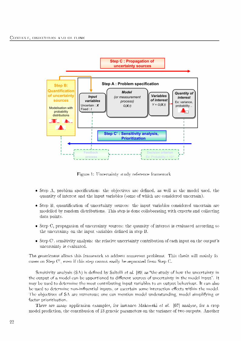
Figure 1 summarizes the referen e framework for un ertainty treatment (de Ro quigny et al.
[30). The breakdown of the study in several steps is done as follows:
21
Context, obje tives and outline
Figure 1: Un ertainty study referen e framework
Step A, problem spe i ation: the obje tives are dened, as well as the model used, the
quantity of interest and the input variables (some of whi h are onsidered un ertain).
Step B, quanti ation of un ertainty sour es: the input variables onsidered un ertain are
modelled by random distributions. This step is done ollaborating with experts and olle ting
data points.
Step C, propagation of un ertainty sour es: the quantity of interest is evaluated a ording to
the un ertainty on the input variables dened in step B.
Step C', sensitivity analysis: the relative un ertainty ontribution of ea h input on the output's
un ertainty is evaluated.
The generi ness allows this framework to address numerous problems. This thesis will mainly fo-
uses on Step C', even if this step annot easily be separated from Step C.
Sensitivity analysis (SA) is dened by Saltelli et al. [89 as the study of how the un ertainty in
the output of a model an be apportioned to dierent sour es of un ertainty in the model input. It
may be used to determine the most ontributing input variables to an output behaviour. It an also
be used to determine non-inuential inputs, or as ertain some intera tion ee ts within the model.
The obje tives of SA are numerous; one an mention model understanding, model simplifying or
fa tor prioritisation.
There are many appli ation examples, for instan e Makowski et al. [67 analyse, for a rop
model predi tion, the ontribution of 13 geneti parameters on the varian e of two outputs. Another
22
example is given in the work of Varet [99 where the aim of SA is to determine the most inuential
inputs among a great number (around 60), for an air raft infrared signature simulation model.
In nu lear engineering eld, Auder et al. [5 study the inuential inputs on thermohydrauli al
phenomena o urring during an a idental s enario, while Iooss et al. [50 and Volkova et al. [100
onsider the environmental assessment of industrial fa ilities.
The rst histori al approa h to sensitivity analysis is known as the lo al approa h. The impa t of
small perturbations of the inputs on the output is studied. These small perturbations o ur around
nominal values (the mean of a random variable for instan e). This is a ounterpart to the partial
derivatives of the model in ertain points of the input spa e. Most of these methods (some of them
will be itemized in se tion 1.3.2) make strong assumptions on the model and/or on the inputs (in
terms of linearity, normality, ...).
A se ond approa h, more re ent due to the development of omputational power is known as
the global approa h. The whole variation range of the inputs is therein onsidered. An appli ative
introdu tion an be found in Iooss [49. Most te hniques (some of them will be dened in se tion
1.3.1 and tested in se tions 1.4 and 1.5) are developed in an independent approa h (model free),
without making assumptions su h as linearity or monotony.
Stru tural reliability
Consider the industrial problem of knowing if a stru ture, subje t to physi al loads or onstraints,
goes undamaged or goes to a state of failure. This will be referred as stru tural reliability. A
trial and measures approa h might be possible, but an be di ult to manage for safety or osts
reason. Within this ontext, omputer models are used in order to assess the safety of omplex
systems. These models are then used as an approximate representation of the reality, in luding
some me hanisms su h as aw propagation, fri tion laws...
In order to ompletely use the model, un ertainties on the model inputs (essentially physi al
values) are modelled by random variables. The model is therefore representing the stru ture gifted
with a ertain toughness and the environment providing a load. Computation for a xed set of
inputs allows to obtain a failure riterion leading to a binary response: for this set of inputs, the
stru ture fails or behaves soundly.
The fa t that un ertainties are modelled by random variables enables risk modelling as a failure
probability. This approa h is more subtle than a deterministi approa h where inputs are xed to
nominal values (generally penalized).
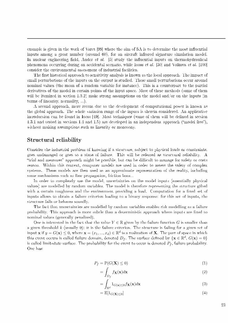
One is interested in the fa t that the value Y ∈ R given by the failure fun tion G is smaller than
a given threshold k (usually 0): it is the failure riterion. The stru ture is failing for a given set of
input x if y = G(x) ≤ 0, where x = (x1, ..., xd) ∈ Rdis a realization of X. The part of spa e in whi h
this event o urs is alled failure domain, denoted Df . The surfa e dened by x ∈ Rd, G(x) = 0is alled limit-state surfa e. The probability for the event to o ur is denoted Pf , failure probability.
One has:
Pf = P(G(X) ≤ 0) (1)
=
Df
fX(x)dx (2)
=
Rd
1G(x)≤0fX(x)dx (3)
= E[1G(X)≤0] (4)
23
Context, obje tives and outline
The omplexity of models and the possible great number of inputs make di ult, in a general
ase, to ompute the exa t value of Pf . However, it an be estimated (sin e written under the form
of a mathemati al expe tation) with the help of several methods that will be itemized in se tion 1.2.
The primer of stru tural safety is to provide an estimation of Pf and some un ertainty surrounding
this estimation. It an be used to answer the original question of the stru ture supporting the loads.
Context: omponent within nu lear rea tor (CWNR)
This ase-study provided the initial motivation for this work. It fo uses on the reliability and risk
analysis of a nu lear power plant omponent. However the results of this thesis must be onsidered
as textbook exer ises, whi h an not be used to draw on lusions about the integrity or safety
assessment of nu lear power plants.
During the normal operation of a nu lear power plant, the omponent within nu lear rea tor
(CWNR) is exposed to ageing me hanisms. In order to assess the integrity of the omponent, it has
been demonstrated that a postulated manufa turing aw an withstand severe me hani al loads.
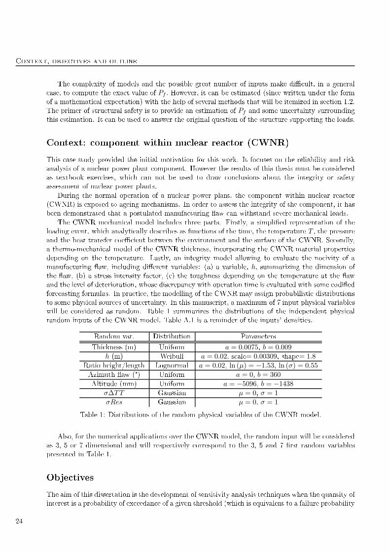
The CWNR me hani al model in ludes three parts. Firstly, a simplied representation of the
loading event, whi h analyti ally des ribes as fun tions of the time, the temperature T , the pressureand the heat transfer oe ient between the environment and the surfa e of the CWNR. Se ondly,
a thermo-me hani al model of the CWNR thi kness, in orporating the CWNR material properties
depending on the temperature. Lastly, an integrity model allowing to evaluate the no ivity of a
manufa turing aw, in luding dierent variables: (a) a variable, h, summarizing the dimension of
the aw, (b) a stress intensity fa tor, ( ) the toughness depending on the temperature at the aw
and the level of deterioration, whose dis repan y with operation time is evaluated with some odied
fore asting formulas. In pra ti e, the modelling of the CWNR may assign probabilisti distributions
to some physi al sour es of un ertainty. In this manus ript, a maximum of 7 input physi al variables
will be onsidered as random. Table 1 summarizes the distributions of the independent physi al
random inputs of the CWNR model. Table A.1 is a reminder of the inputs' densities.
Random var. Distribution Parameters
Thi kness (m) Uniform a = 0.0075, b = 0.009
h (m) Weibull a = 0.02, s ale= 0.00309, shape= 1.8
Ratio height/length Lognormal a = 0.02, ln (µ) = −1.53, ln (σ) = 0.55
Azimuth aw (°) Uniform a = 0, b = 360
Altitude (mm) Uniform a = −5096, b = −1438
σ∆TT Gaussian µ = 0, σ = 1
σRes Gaussian µ = 0, σ = 1
Table 1: Distributions of the random physi al variables of the CWNR model.
Also, for the numeri al appli ations over the CWNR model, the random input will be onsidered
as 3, 5 or 7 dimensional and will respe tively orrespond to the 3, 5 and 7 rst random variables
presented in Table 1.
Obje tives
The aim of this dissertation is the development of sensitivity analysis te hniques when the quantity of
interest is a probability of ex eedan e of a given threshold (whi h is equivalent to a failure probability
24
in the eld of stru tural reliability). The onstraints of the CWNR ode are to be taken into a ount.
The expe ted magnitude of the failure probability is less than 10−5. If possible, the methods must
be related to the estimation of Pf and must provide an estimation of the error made when estimating
sensitivity indi es as well as an estimation of the error made when estimating Pf .
Outline
The following thesis is organised in four hapters.
The rst hapter is an overview of both existing strategies for estimating failure probabilities and
methods of sensitivity analysis. In this hapter, states of the art for reliability and sensitivity analysis
(SA) te hniques will be separately developed. More pre isely, three main families of reliability
te hniques will be studied: Monte-Carlo methods, stru tural reliability methods and sequential
Monte-Carlo methods. Finally, two families of well-known sensitivity analysis te hniques will be put
to the proof on reliability test ases (whi h are itemized in Appendix B). These te hniques show
some limitations, onrming the need to develop SA methods fo used on failure probabilities. A
table (Table 1.13) summarizing the presented methods is proposed, and a dis ussion on the meaning
of sensitivity analysis in the reliability ontext is ondu ted.
The se ond hapter fo uses on dening measures of sensitivity in order to produ e a variable
ranking. More spe i ally, the use of random forests on a Monte-Carlo sample is proposed in the
rst pla e. Two importan e measures derived from the random forests predi tors are tested on the
usual ases. In the se ond pla e, a te hnique using a sample produ ed by sequential Monte-Carlo
methods is eli ited. This last method is based on the departure between the marginal distribution
of an input and its equivalent given the step of the subset method.
The third hapter presents an original method to estimate the importan e of ea h variable on
a failure probability. This method fo uses on the impa t of perturbations upon the original input
densities fi. A general framework dening appropriate perturbations is elaborated, then sensitivity
indi es are presented. An estimation te hnique of these indi es that makes no further alls to the
model is given. The methodology is then tested on the usual ases.
The fourth hapter presents the appli ation of the developed methods to the CWNR ase. Several
tunings will be studied to assess or inrm the ability of the dierent SA methods to identify inuential
variables.
25

Chapter 1
State of the art for reliability and
sensitivity analysis
1.1 Introdu tion
The outline of the hapter is the following: in Se tion 1.2, a state of the art for reliability is proposed.
Several te hniques for estimating failure probabilities are presented. Then in Se tion 1.3, a review
of Sensitivity Analysis (SA) is given. The appli ation of a well-known SA method, Sobol' indi es
(1.3.1.3) on a failure probability, is tested on numerous appli ation ases in Se tion 1.4. In Se tion
1.5, the so- alled moment independent sensitivity measures (presented in Se tion 1.3.1.4) are tested
within the reliability ontext. Next, Se tion 1.6 proposes a synthesis of these states of the art.
Finally, Se tion 1.7 dis usses the meaning and obje tives of sensitivity analysis when dealing with
failure probabilities.
1.2 State of the art: reliability and failure probability estimation
te hniques
This state of the art for reliability is widely inspired by the PhD thesis of Gille-Genest [41, Can-
naméla [22 (in Fren h) and Dubourg [33 (in English). In addition, monographs by Madsen et al.
[66 and Lemaire [60 have been used. In this se tion, a state of the art for the estimation te hniques
of failure probabilities is detailed. Choi e is set to present 3 families of methods.
Monte-Carlo (MC) simulation methods: these te hniques are standard in statisti s. The MC
methods are used to estimate an expe tation. These are based upon an appli ation of the
Strong Law of Large Numbers for estimation and on the Limit Central Theorem for error
ontrol. Several varian e-redu tion te hniques are available in the literature. The most appro-
priate of them will be itemised in 1.2.1.
Reliability methods: histori ally these methods ome from me hani al engineering. They
provide answers based upon a linear (FORM) or quadrati (SORM) approximation of the
failure surfa e. This approximation is then used to estimate the failure probability. As far as
we know, error ontrol is not easily made. These methods are presented in 1.2.2.
Subset simulation methods: sometimes also referred as parti le methods, sequential MC or
splitting te hniques, these methods have been more re ently developed. They are based upon
a de omposition of the obje tive probability as a produ t of onditional probabilities, that
27
1. State of the art for reliability and sensitivity analysis
are easier to estimate. These estimations are made running a large number of Monte-Carlo
Markov Chains (MCMC). Some te hniques will be presented in 1.2.3.
However, the partition must be qualied. In pra ti e, methods an be asso iated; for instan e one
an rst use FORM numeri al approximation, then perform some importan e sampling around the
most probable failing point. In the same way, most of Munoz-Zuniga's works [72 are devoted to a
stratied sampling te hnique (MC varian e-redu tion method) ombined with dire tional simulation.
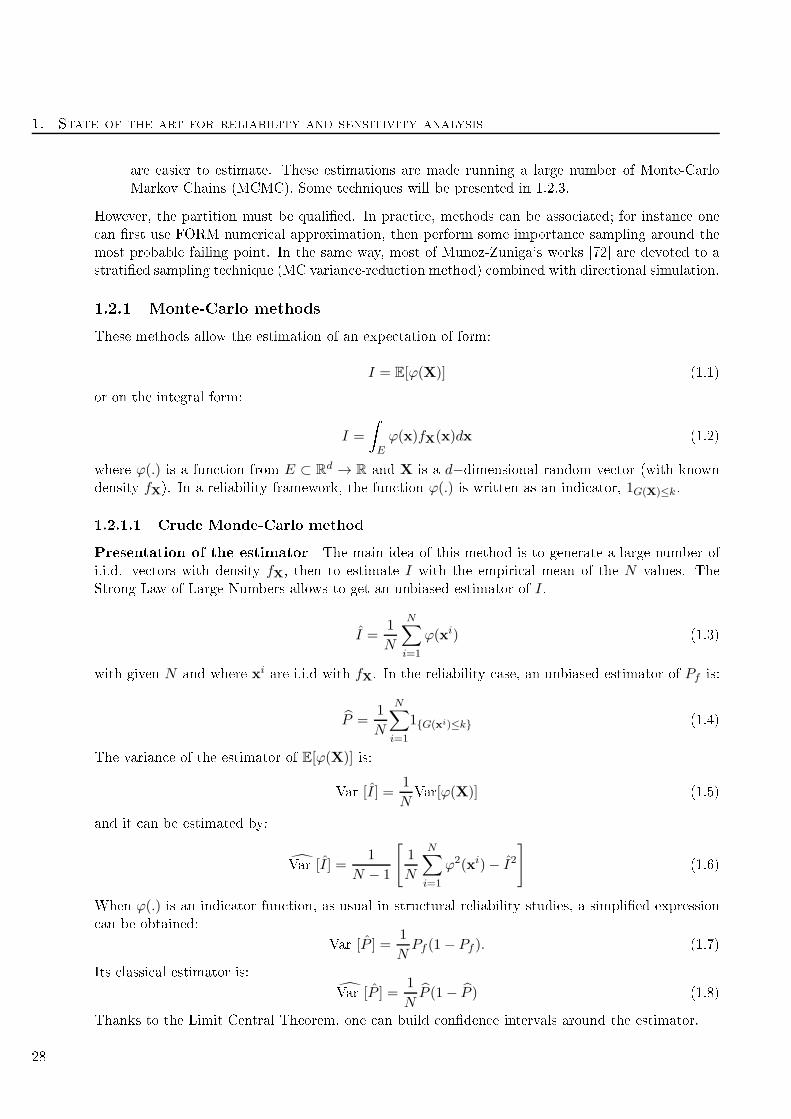
1.2.1 Monte-Carlo methods
These methods allow the estimation of an expe tation of form:
I = E[ϕ(X)] (1.1)
or on the integral form:
I =
Eϕ(x)fX(x)dx (1.2)
where ϕ(.) is a fun tion from E ⊂ Rd → R and X is a d−dimensional random ve tor (with known
density fX). In a reliability framework, the fun tion ϕ(.) is written as an indi ator, 1G(X)≤k.
1.2.1.1 Crude Monde-Carlo method
Presentation of the estimator The main idea of this method is to generate a large number of
i.i.d. ve tors with density fX, then to estimate I with the empiri al mean of the N values. The
Strong Law of Large Numbers allows to get an unbiased estimator of I.
I =1
N
N∑
i=1
ϕ(xi) (1.3)
with given N and where xiare i.i.d with fX. In the reliability ase, an unbiased estimator of Pf is:
P =1
N
N∑
i=1
1G(xi)≤k (1.4)
The varian e of the estimator of E[ϕ(X)] is:
Var [I ] =1
NVar[ϕ(X)] (1.5)
and it an be estimated by:
Var [I] =1
N − 1
[1
N
N∑
i=1
ϕ2(xi)− I2
](1.6)
When ϕ(.) is an indi ator fun tion, as usual in stru tural reliability studies, a simplied expression
an be obtained:
Var [P ] =1
NPf (1− Pf ). (1.7)
Its lassi al estimator is:
Var [P ] =1
NP (1− P ) (1.8)
Thanks to the Limit Central Theorem, one an build onden e intervals around the estimator.
28
1.2. State of the art: reliability and failure probability estimation te hniques
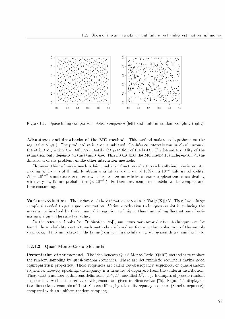
Figure 1.1: Spa e lling omparison: Sobol's sequen e (left) and uniform random sampling (right).
Advantages and drawba ks of the MC method This method makes no hypothesis on the
regularity of ϕ(.). The produ ed estimator is unbiased. Conden e intervals an be obtain around
the estimator, whi h are useful to quantify the pre ision of the latter. Furthermore, quality of the
estimation only depends on the sample size. This means that the MC method is independent of the
dimension of the problem, unlike other integration methods.
However, this te hnique needs a fair number of fun tion alls to rea h su ient pre ision. A -
ording to the rule of thumb, to obtain a variation oe ient of 10% on a 10−kfailure probability,
N = 10k+2simulations are needed. This an be unrealisti in some appli ations when dealing
with very low failure probabilities (< 10−6). Furthermore, omputer models an be omplex and
time- onsuming.
Varian e-redu tion The varian e of the estimator de reases in Var[ϕ(X)]/N . Therefore a large
sample is needed to get a good estimation. Varian e-redu tion te hniques onsist in redu ing the
un ertainty involved by the numeri al integration te hnique, thus diminishing u tuations of esti-
mations around the sear hed value.
In the referen e books (see Rubinstein [85), numerous varian e-redu tion te hniques an be
found. In a reliability ontext, su h methods are based on fo using the exploration of the sample
spa e around the limit state (ie, the failure) surfa e. In the following, we present three main methods.
1.2.1.2 Quasi Monte-Carlo Methods
Presentation of the method The idea beneath Quasi Monte-Carlo (QMC) method is to repla e
the random sampling by quasi-random sequen es. These are deterministi sequen es having good
equirepartition properties. These sequen es are alled low-dis repan y sequen es, or quasi-random
sequen es. Loosely speaking, dis repan y is a measure of departure from the uniform distribution.
There exist a number of dierent denitions (L∞, L2, modied L2, . . . ). Examples of pseudo-random
sequen es as well as theoreti al developments are given in Niederreiter [75. Figure 1.1 displays a
two-dimensional example of better spa e lling by a low-dis repan y sequen e (Sobol's sequen e),
ompared with an uniform random sampling.
29
1. State of the art for reliability and sensitivity analysis
QMC estimation of the desired quantity is obtained substituting in the MC estimator the random
samples by the pseudo-random samples. However, it is not possible to obtain a varian e estimation of
the QMC estimator. Koksma-Hlakwa's inequality allows to bound the error made when integrating
with QMC method, depending on the hosen sequen e and on ϕ(.)'s regularity.
Reliability ase QMC methods are not well adapted for stru tural reliability. The main issue
when estimating small failure probabilities by MC is to get extreme samples (within the distribution
tail) leading to the failure event, rather than getting evenly distributed samples. However, these
methods will be applied in Se tion 1.4 to de rease the number of fun tion alls when estimating
Sobol' indi es (whi h are dened in Se tion 1.3.1.3).
1.2.1.3 Importan e sampling
Presentation of the method The basi idea of importan e sampling is to modify the sampling
density. The estimator is then obtained by in luding a density ratio. The aim is to foster sampling
in signi ant regions. In a reliability ontext, this is simply in reasing the number of failure samples.
Let us denote fX
a density sele ted by the pra titioner. It will be referred to as the instrumental
density. The problem rewrites as follows:
I =
Eϕ(x)fX(x)dx (1.9)
=
Eϕ(x)
fX(x)
fX(x)
fX(x)dx (1.10)
= EX
[ϕ (X)
fX(x)
fX(x)
](1.11)
where EXis the expe tation when X is of density f
X. The estimation is then made by:
IIS =1
N
N∑
i=1
ϕ(xi)fX(x
i)
fX(xi)
(1.12)
where xiare i.i.d with density f
X. One an also get the varian e of the estimator:
Var(IIS) =1
NVar
X
[ϕ(X)
fX(X)
fX(X)
](1.13)
where Var
Xis the varian e when X follows density f
X. It should be noti ed that the support of f
X
must be in luded within the support of the initial density fX. Otherwise, the estimator is biased.
This te hnique does not onsistently provide a varian e redu tion. A given instrumental density
fXuseful only if:
Var
X
[ϕ(X)
fX(X)
fX(X)
]< VarX[ϕ(X)] (1.14)
Minimal varian e is obtained with the following optimal density:
fX∗(x) =|ϕ(x)|fX(x)
|ϕ(y)|fX(y)dy(1.15)
However, the denominator on the latter is di ult to estimate as it boils down to I in the ase of a
positive fun tion ϕ(.). Choosing of a well-tted instrumental density is a problem in itself. Chapter
2 of Cannaméla [22 provides a state of the art of sele ting a quasi-optimal instrumental density.
30
1.2. State of the art: reliability and failure probability estimation te hniques
Reliability ontext The estimator of Pf is:
PIS =1
N
N∑
i=1
1G(xi)≤kfX(x
i)
fX(xi)
(1.16)
Thus the optimal density an be rewritten as:
fX∗(x) =1x∈Df fX(x)
DffX(y)dy
=1x∈DffX(x)
Pf= fX(x|Df ) (1.17)
This density is intra table in pra ti e, Pf being the quantity of interest. Choi e of a good instru-
mental density is therefore a problem in reliability as well. One an quote hapter 5 of Munoz
Zuniga [72 in whi h an adaptive and non parametri te hnique for instrumental density sele tion
(adapted to this reliability ontext) is presented. Additionally, Pastel [79 developed an interesting
non-parametri adaptive te hnique, still within the reliability framework.
1.2.1.4 Dire tional sampling
In pra ti e this te hnique is spe i to stru tural reliability studies.
Prin iple First, the random input ve tor is transformed into a random ve tor for whi h all om-
ponents are standard Gaussian random variables. This is also referred as transforming the physi al
spa e into the standard Gaussian spa e (sometimes referred to as U-spa e). Su h an isoprobabilisti
transformation T whi h turns the random ve tor X of density fX into a random ve tor whose all
omponents are independent standard Gaussians. Given X = (X1, ...,Xd) the random input ve tor,
one obtains U = (U1, .., Ud) = T (X) where Ui, i = 1, ..., d are independent standard Gaussians. Let
us denote:
H(u) = G(T−1(u)) = G(x). (1.18)
Several isoprobabilisti transformations exist. Nataf, generalized Nataf and Rosenblatt transforma-
tions (see Lebrun and Dutfoy [58, 59) are the most adapted. The latter is developed in Appendix
C. On e the transformation is done, the quantity of interest an be rewritten as:
Pf = P(H(U) ≤ k). (1.19)
The main idea of this method is to generate dire tions from the enter of the standard Gaussian
spa e in a uniform and independent way. Then, the failure fun tion is omputed along the dire tions.
Given the dire tion, this allows a onditional estimation of the failure probability. Ve tor U an be
rewritten as a produ t:
U = RA
with R ≥ 0, R² following a χ2distribution with d degrees of freedom and A an uniform random
variable on the unit sphere Ωd, independent of R. Denoting fA the uniform density on Ωd, one an
rewrite the failure probability onditionally to the dire tions:
Pf =
Ωd
P(H(Ra) ≤ k)fA(a)da (1.20)
31
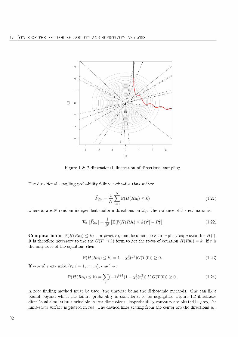
1. State of the art for reliability and sensitivity analysis
Figure 1.2: 2-dimensional illustration of dire tional sampling
The dire tional sampling probability failure estimator thus writes:
Pdir =1
N
N∑
i=1
P(H(Rai) ≤ k) (1.21)
where ai are N random independent uniform dire tions on Ωd. The varian e of the estimator is:
Var[Pdir] =1
N
[E[P(H(RA) ≤ k))2]− P 2
f
](1.22)
Computation of P(H(Rai) ≤ k) In pra ti e, one does not have an expli it expression for H(.).It is therefore ne essary to use the G(T−1(.)) form to get the roots of equation H(Rai) = k. If r isthe only root of the equation, then:
P(H(Rai) ≤ k) = 1− χ2d(r
2)G(T (0)) ≥ 0. (1.23)
If several roots exist (ri, i = 1, . . . , n), one has:
P(H(Rai) ≤ k) =∑
i
(−1)i+1(1− χ2d(r
2i )) if G(T (0)) ≥ 0. (1.24)
A root nding method must be used (the simplest being the di hotomi method). One an x a
bound beyond whi h the failure probability is onsidered to be negligible. Figure 1.2 illustrates
dire tional simulation's prin iple in two dimensions. Isoprobability ontours are plotted in grey, the
limit-state surfa e is plotted in red. The dashed lines staring from the enter are the dire tions ai.
32

1.2. State of the art: reliability and failure probability estimation te hniques
1.2.2 Stru tural reliability methods
1.2.2.1 Reliability indi es
Reliability indi es give indi ations about the relative weights of input parameters in the whole
reliability of the onsidered stru ture(they are also sometimes alled safety index). They allow a
omparison of several setups possible. The larger the index, the safer the stru ture. In the following,
two indi es are presented.
Hasofer-Lind index Proposed by Hasofer and Lind in 1974 [43, it is an exa t geometri index,
invariant with respe t to the geometry of the limit state surfa e. It is dened in the Gaussian
standard spa e. Let us dene the most probable failure point as the losest failure point to the
origin of the standard spa e (the origin of the standard spa e is onsidered outside of the failure
domain). Su h a point is also referred as a design point. Assuming the design point is unique, one
an dene the Hasofer-Lind index as the distan e between the origin and the design point:
βHL = minH(u)=0
(uTu)1/2 (1.25)
Algorithms to nd su h design points are numerous, one an quote the Hasofer-Lind-Ra kwitz-
Fiessler algorithm [82 and its improved version iHLRF (Zhang and Der Kiureghian, [102). One an
also quote a work arried out at EDF R&D about testing the quality of a design point (Dutfoy and
Lebrun,[34). Further details on design point nding algorithms are given in se tion 1.2.2.2. One
should note that an estimation of the Hasofer-Lind index does not require an estimation of Pf but
only an estimated design point.
Generalized reliability index The generalized reliability index was proposed by Ditlevsen in
1979 [32 to take a ount of the urvature of the failure surfa e around the design point. Dening
a reliability measure γ by integrating a weight fun tion (in pra ti e the d-dimensional standard
Gaussian distribution) over the safe set S:
γ =
SϕddS. (1.26)
The generalized reliability index is dened as a monotoni ally in reasing fun tion of γ:
βG = Φ−1(γ) (1.27)
where Φ−1is the inverse umulative distribution fun tion of the standard Gaussian. One an estimate
the index by:
βG = Φ−1(1− P ) (1.28)
where P is an estimation of the failure probability (obtained for instan e through MC integration or
by FORM/SORM, see se tion 1.2.2.2). This index equals the Hasofer-Lind one if the failure surfa e
is an hyperplane in the standard Gaussian spa e. Finally, the estimation of this index requires an
estimation of the failure probability Pf .
1.2.2.2 FORM-SORM methods
The First Order Reliability Method (FORM) and Se ond Order Reliability Method (SORM) are
estimation te hniques for a failure probability based upon integration of an approximation of the
failure surfa e. In pra ti e, they are onsidered as a standard solution in stru tural reliability sin e
they are not ostly, easy to understand and to implement.
These methods pro eed in four steps:
33
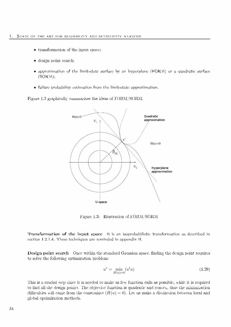
1. State of the art for reliability and sensitivity analysis
transformation of the input spa e;
design point sear h;
approximation of the limit-state surfa e by an hyperplane (FORM) or a quadrati surfa e
(SORM);
failure probability estimation from the limit-state approximation.
Figure 1.3 graphi ally summarises the ideas of FORM/SORM.
Figure 1.3: Illustration of FORM/SORM
Transformation of the input spa e It is an isoprobabilisti transformation as des ribed in
se tion 1.2.1.4. These te hniques are reminded in appendix B.
Design point sear h On e within the standard Gaussian spa e, nding the design point requires
to solve the following optimization problem:
u∗ = minH(u)=0
(utu) (1.29)
This is a ru ial step sin e it is needed to make as few fun tion alls as possible, while it is required
to nd all the design points. The obje tive fun tion is quadrati and onvex, thus the minimization
di ulties will ome from the onstraints (H(u) = 0). Let us make a distin tion between lo al and
global optimization methods.
34
1.2. State of the art: reliability and failure probability estimation te hniques
Lo al methods Lo al minima sear h is e ient if one has an expli it expression of the
gradient of H. This is seldom the ase in industrial appli ations and one has to use approximations
based upon nite dieren es. These approximations may be ostly in terms of fun tion alls, and
they an lead to a loss of onvergen e of the algorithms. Most algorithms sear h for the optimum u∗
in an iterative way. The idea is, starting from a given point u(k), to nd the best des ent dire tion
d(k) and the best length of the step α(k):
u(k+1) = u(k) + α(k)d(k). (1.30)
The iteration an be followed by a proje tion.
Numerous methods are des ribed in Lemaire [60, whi h are divided in 4 main ategories : zero
order methods, rst order methods, se ond order methods and hybrid methods. Zero order methods
(di hotomy for instan e) does not require a omputation of the gradient. However their onvergen e
is slow. In the reliability ase, this implies a large number of fun tion alls. Thus these zero order
methods are not adapted to reliability problems onsidered in this thesis
Here is presented the rst order Hasofer-Lind-Ra kwitz-Fiessler (HL-RF) algorithm. It has been
developed spe i ally for reliability studies. Its onvergen e is not assured but the method is ee tive
in many ases. It is worth noti ing that the algorithm has been adapted to led to onvergen e
improvements (Abdo and Ra kwitz [1). The iteration is as follows:
u(k+1) = (u(k)tβ(k))β(k) − H(u(k))
||∇H(u(k))||β(k)
with β(k) =∇H(u(k))
||∇H(u(k))|| (1.31)
Global methods If the limit-state surfa e presents several design points, the previously de-
s ribed algorithms may not identify these design points. Der Kiureghian and Dakessian [31 proposed
to for e the onvergen e of the HL-RF algorithm to a new design point by disturbing the vi inity of
the previously found design point.
Approximation of the limit-state surfa e FORM method repla es the limit-state surfa e by a
hyperplane tangent at the design point. A loss of pre ision depending on the form of the limit-state
surfa e at the design point o urs. If the limit-state surfa e is lose from the hyperplane, this method
provides good pre ision ompared to the needed number of fun tion alls. The linear approximation
writes as follows:
∇H(u)t|u=u∗(u− u∗) = 0 (1.32)
The SORMmethod repla es the limit-state surfa e by a se ond-order (quadrati ) hypersurfa e. Su h
a method requires the estimation of the urvature of the limit-state surfa e at the design point u∗.Several te hniques are provided in Lemaire [60. The key message is that the use of SORM over
FORM is justied when it is known that the surfa e is almost quadrati .
Failure probability estimation In the FORM approximation, one uses the Hasofer-Lind relia-
bility index presented in se tion 1.2.2.1 and estimates Pf with:
PFORM = 1− Φ(βHL) (1.33)
SORM approximation is a more omplex problem, for whi h an asymptoti approximation was
provided by Breitung [18.
35

1. State of the art for reliability and sensitivity analysis
On the geometri approximations FORM/SORM te hniques are popular methods in the do-
main of stru tural reliability, be ause a few fun tion alls are needed to get an estimation of Pf .
Also, FORM is easy to understand and to implement. However, a signi ant error an be made
when using FORM. Consequently, these methods should only be used when it is known that the
limit-state surfa e has a given geometri al shape (almost hyperplane or almost quadrati ). Su h an
information is not always available.
1.2.3 Subset simulation
1.2.3.1 Introdu tion
Subset simulation methods are based upon a division of the failure probability in a produ t of
onditional probabilities. These are larger therefore easier to estimate. Let us onsider a sequen e
of M + 1 thresholds T su h as:
T = +∞, t1, ..., tM = 0and let us also dene the sequen e of nested subsets (also sometimes referred to as intermediate
failure events):
Ak = x|G(x) < tk.One has:
P [x ∈ Ak] =
k∏
i=1
P [x ∈ Ai|x ∈ Ai−1]
and one an rewrite Pf as:
Pf = P [x ∈ AM ] =M+1∏
i=1
P [x ∈ Ai|x ∈ Ai−1] (1.34)
thus the estimation of Pf is redu ed to the estimation of the onditional failure probabilities. The
name subset simulation has been introdu ed by Au and Be k [4. For the sake of simpli ity, let us
denote:
P(Ak) = P [x ∈ Ak]
and
P(Ak|Ak−1) = P [x ∈ Ai|x ∈ Ai−1] .
The algorithm rst step is to estimate P(A1) by standard Monte Carlo simulation. One has:
P (A1) =1
N
N∑
k=1
1G(xi)<t1
where xiare i.i.d. to f . MCMC te hniques are thereafter used to estimate the onditional failure
probabilities P(Ak|Ak−1), k = 2, . . . ,M . Let us denote:
f(x|Ai) =f(x)1G(x)<ti
P (Ai)(1.35)
the onditional density of x given that the i−th threshold has been rea hed. The goal of the
algorithms displayed in the following is to sample a ording to this obje tive distribution. As the
denominator is an unknown quantity, indire t sampling of the obje tive distribution is needed, whi h
is pra ti ally made using Monte Carlo Markov Chains (MCMC).
36

1.2. State of the art: reliability and failure probability estimation te hniques
1.2.3.2 Algorithm
A so- alled modied Metropolis algorithm is presented in the Au and Be k's [4 original arti le. The
modi ation is operated to allow the pra titioner to deal with high-dimensional densities. Let us
rst re all the Metropolis algorithm.
Metropolis algorithm Let us denote a proposal density p∗(ǫ|x), a joint d−dimensional density,
entred in x with a symmetry property p∗(ǫ|x) = p∗(x|ǫ). We are interested in the produ tion of
the sample x(i+1), lying in the subset Ak. It is generated starting from the initial sample x(i) ∈ Ak
as follows:
Sampling of the andidate sample x: ǫ is simulated a ording to p∗(ǫ|x(i)). Ratio r =f(ǫ)/f(x(i)) is omputed. The andidate sample is x = ǫ with probability min(1, r) and
stays x = x(i)with probability 1−min(1, r).
A eptan e/reje tion of the andidate x: one he ks that x lies within the interest zone Ak.
If G(x) < sk then x(i+1) = x. Else, x(i+1) = x(i).
A ording to the authors, this algorithm is not robust to the large dimension, given a high reje tion
rate. This reje tion rate implies a high orrelation within the produ ed samples, thus redu ing the
e ien y of the simulation pro ess. The authors then propose a modied Metropolis algorithm to
ope with the simulation of random ve tors of high dimension.
Modied Metropolis algorithm For all dimensions j = 1, . . . , d let us denote p∗j(ǫ|xj), a
1−dimensional proposal density, entred in xj with a symmetry property p∗j(ǫ|xj) = p∗j(xj |ǫ). Thesample x(i+1)
, lying in the subset Ak, is generated starting from the initial sample x(i) ∈ Ak as
follows:
Sampling of the andidate sample x: for ea h omponent j, let us sample ǫj a ording to
p∗j(ǫ|x(i)j ). Ratio rj = fj(ǫ)/fj(x
(i)j ) is omputed. Candidate's j−th omponent is thus xj = ǫj
with probability min(1, rj) and is xj = x(i)j with probability 1−min(1, rj).
A eptan e/reje tion of the andidate x: one he ks that x lies within the interest zone Ak.
If G(x) < sk then x(i+1) = x. Else, x(i+1) = x(i).
The authors show that the Markov hain generated through this algorithm has stationary distri-
bution f(x|Ak). The hoi e of proposal density is important, the authors state that the method is
more sensible to the spread of the proposal densities than to their stru tural form (e.g., Gaussian,
gamma, et .). Based on this observation, the authors re ommend to use uniform densities.
On the threshold hoi e The authors a knowledge that the hoi e of the threshold is essential
in the simulation pro ess. Thus, their advi e is to hoose an adaptive hoi e of the threshold so that
the onditional probabilities P(Ak|Ak−1) are xed.
1.2.3.3 Theoreti al results and strategies
Cérou et al. [23 present, from a theoreti al point of view, two strategies to estimate small failure
probabilities. The dieren e between these two methods lies in the adaptive sele tion of the threshold
for the se ond.
37
1. State of the art for reliability and sensitivity analysis
Fixed levels algorithm The authors onsider a transition Markov kernel K on Rdwhi h is
f -symmetri (thus f -invariant):
f(dx)K(x, dy) = f(dy)K(y, dx).
A Metropolis-Hasting kernel is proposed (as in Au and Be k [4). The authors then onsider a
Markov hain (Xk)k≥0 su h that the initial density is f . The generation algorithm is as follows: a
parti le loud of size N is sampled, one has X(j)0 ∼ f , j = 1, . . . , N . For ea h level k = 1, . . . ,M ,
let us denote Ik+1 the indi es of the parti les that rea h the level of interest:
Ik+1 = j|X(j)k ∈ Ak+1
onditional probability P(Ak+1|Ak) is estimated by pk+1 =|Ik+1|N . For the j of Ik+1, X
(j)k+1 = X
(j)k
is proposed. For the j that are not in Ik+1, X(j)k+1 is randomly hosen (uniformly) as a opy of one
of the parti le in Ik+1. Thus ea h parti le of
(Xk+1
)lies in Ak+1. Then for ea h parti le indexed
by j = 1, . . . , N , transition is twofold. First step is to mutate (or shake) the parti le by applying
(potentially several times) kernel K, produ ing the andidate parti le Z:
Z ∼ K(X(j)k+1, .)
The se ond step is a post-mutation sele tion X(j)k+1 = Z if Z ∈ Ak+1, X
(j)k+1 = X
(j)k+1 else. The parti le
loud is then distributed a ording to f(x|Ak+1). Failure probability Pf is then estimated by the
produ t of the estimators of the onditional probabilities:
P =M∏
k=1
pk (1.36)
The authors show the asymptoti normality of P .
√NP − Pf
Pf
L−−−−→N→∞
N (0, σ2) (1.37)
where σ2 has a omplex expression, given in se tion 2.3 of Cérou et al. [23.
Adaptive levels algorithm The estimator produ ed by the xed levels algorithm rea hes minimal
varian e when the levels are evenly spa ed (in probability), see Lagnoux [56. The authors then
propose another algorithm xing the levels on the y (adaptively). Let us onsider a number
α ∈ [0, 1], su ess rate between two levels. At ea h step, the threshold set is the α-quantile (or theαN parti les whi h G(.) values are the smallest) of the urrent sample. The algorithm stops when
the α-quantile of the sample is lower than 0. One noti es that the number of steps is a random
variable. However, for a loud size N large enough, the number of steps is:
ns = ⌊ log Pf
logα⌋ (1.38)
The authors also show the asymptoti normality of P .
√N(P − Pf
) L−−−−→N→∞
N (0, σ2) (1.39)
where σ2 = P 2(ns
1−αα + 1−r0
r0
)with r0 = Pα−ns
. The estimator P is biased. This bias is positive
and de reases with a
1N rate. However, the adaptive algorithm is more e ient than the xed levels
algorithm, in terms of mean square error (MSE).
38
1.3. Sensitivity analysis (SA)
On the tuning of parameters In the following, the adaptive algorithm presented in Cérou et
al. [23 will be used. Several parameters are yet to be tuned: N , α and the Markov kernel (or
proposal density) hoi e. Balesdent et al. [7 also re ommend to tune the number of appli ation of
the kernel.
For the α, authors of Cérou et al. [23 re ommend to take α of order 0.75. On the other hand,
authors of Au and Be k [4 propose to take α of order 0.1. Unless otherwise mentioned, we
have hosen to take α = 0.75.
The hoi e ofN depends on the studied problem and on the omplexity of the studied numeri al
model. Unless otherwise mentioned, we have hosen to take N = 104.
The hoi e of the Markov kernel (or proposal density) is the most ru ial point. Both arti les
[4 and [23 let the pra titioner hoose the parameter a ording to the problem. The hosen
density will be given for ea h example.
1.3 Sensitivity analysis (SA)
In this se tion, the main methods of SA will be developed. The motivations have been presented
in page 22. Additionally, a deeper dis ussion of these motivations, that proposes new guidelines for
ondu ting SA for failure probabilities is provided in se tion 1.7.
1.3.1 Global sensitivity analysis
Global SA methods are used to identify the inputs ontributing to the output variability, onsidering
the whole input support. The methods presented in this subse tion, whi h is inspired by Iooss [49,
are divided into four main lasses. The rst will be the s reening methods, designed to deal with
a large number of inputs. The se ond lass is omposed of the methods based on the analysis of
linear models, where a linear model is tted and its by-produ ts are used to perform SA. The third
lass ontains methods based on a varian e de omposition of the output. Finally, some moment-
independent methods will be presented in the fourth lass.
1.3.1.1 S reening methods
S reening methods are based on a dis retisation of the inputs in levels, allowing a qui k exploration
of the ode behaviour. These methods are adapted to a fair number of inputs; pra ti e has often
shown that only a small number of inputs are inuential. The hoi e has been made to present
Morris method [71. The aim of this type of method is to identify the non-inuential inputs in a
small number of model alls. The model is therefore simplied before using other SA methods, more
subtle but more ostly.
The method of Morris allows to lassify the inputs in three groups: inputs having negligible
ee ts; inputs having linear ee ts without intera tions and inputs having non-linear ee ts and/or
with intera tions. The method onsists of dis retising the input spa e for ea h variable, then per-
forming a given number of OAT designs (one-at-a-time design of experiments, in whi h only one
input varies). Su h designs of experiments are randomly hosen in the input spa e, and the variation
dire tion is also random. The repetition of these steps allows the estimation of elementary ee ts
for ea h input. From these ee ts are derived sensitivity indi es.
Let us denote r the number of OAT designs (Saltelli et al. [89 propose to set parameter rbetween 4 and 10). Let us dis retise the input spa e in a d−dimensional grid with n levels per
39
1. State of the art for reliability and sensitivity analysis
input. Let us denote E(i)j the elementary ee t of the j−th variable obtained at the i−th repetition,
dened as:
E(i)j =
G(X(i) +ej)−G(X(i))
(1.40)
where is a predetermined multiple of
1(n−1) and ej a ve tor of the anoni al base. Indi es are
obtained as follows:
µ∗j =1
r
r∑
i=1
|E(i)j | (mean of the absolute value of the elementary ee ts),
σj =
√√√√1
r
r∑
i=1
(E
(i)j − 1
r
r∑
i=1
E(i)j
)2
(standard deviation of the elementary ee ts).
The interpretation of the indi es is the following:
µ∗j is a measure of inuen e of the j−th input on the output. The larger µ∗j is, the more the
j−th input ontributes to the dispersion of the output.
σj is a measure of non-linear and/or intera tion ee ts of the j−th input. If σj is small,
elementary ee ts have low variations on the support of the input. Thus the ee t of a
perturbation is the same all along the support, suggesting a linear relationship between the
studied input and the output. On the other hand, the larger σj is, the less likely the linearity
hypothesis is. Thus a variable with a large σj will be onsidered having non-linear ee ts, or
being implied in an intera tion with at least one other variable.
Then, a graph linking µ∗j and σj allows to distinguish the 3 groups.
1.3.1.2 Methods based on the analysis of linear models
If a sample of inputs and outputs large enough is available, it is possible to t a linear model
explaining the behaviour of Y given the values of the random ve tor X. Global sensitivity measures
dened through the study of the tted model are available and presented in the following. Statisti al
te hniques allow to onrm the linear hypothesis. If the hypothesis is reje ted, but that the monotony
of the model is onrmed, one an use the same measures using a rank transformation. Main indi es
are:
Pearson orrelation oe ient:
ρ(Xj , Y ) =
∑Ni=1(X
(i)j − E(Xj))(Yi − E(Y ))
√√√√N∑
i=1
(X
(i)j − E(Xj)
)2√√√√
N∑
i=1
(Yi − E(Y ))2
. (1.41)
It an be seen as a linearity measure between variable Xj and output Y . It equals 1 or −1 if thetested input variable has a linear relationship with the output. If Xj and Y are independent,
the index equals 0.
40

1.3. Sensitivity analysis (SA)
Standard Regression Coe ient (SRC):
SRCj = βj
√Var(Xj)
Var(Y )(1.42)
where βj is the linear regression oe ient asso iated to Xj . SRC2j represents a share of vari-
an e if the linearity hypothesis is onrmed.
Partial Correlation Coe ient (PCC):
PCCj = ρ(Xj − X−j , Y − Y−j) (1.43)
where X−j is the predi tion of the linear model, expressing Xj with respe t to the other inputs
and Y−j is the predi tion of the linear model where Xj is absent. PCC measures the sensitivity
of Y to Xj when the ee ts of the other inputs have been an elled.
1.3.1.3 Fun tional de omposition of varian e : Sobol' indi es
When the model is non-linear and non-monotoni , the de omposition of the output varian e is still
dened and an be used for SA. Let us have f(.) a square-integrable fun tion, dened on the unit
hyper ube [0, 1]d. It is possible to represent this fun tion as a sum of elementary fun tions (Hoeding
[46):
G(X) = G0 +
d∑
i=1
Gi(Xi) +
d∑
i<j
Gij(Xi,Xj) + · · ·+G12...d(X) (1.44)
This expansion is unique under ondition (Sobol' [92):
1
0Gi1...is(xi1 , ..., xis)dxik = 0 , 1 ≤ k ≤ s, i1, ..., is ⊆ 1, ..., d .
This implies that G0 is a onstant.
In the SA framework, let us have X = (X1,...,Xd), a random ve tor where the variables are
mutually independent and Y = G(X), output of a deterministi ode G(). Thus a fun tional
de omposition of the varian e is available, often referred as fun tional ANOVA:
Var[Y ] =
d∑
i=1
Di(Y ) +
d∑
i<j
Dij(Y ) + · · ·+D12...d(Y ) (1.45)
where Di(Y ) = Var[E(Y |Xi)], Dij(Y ) = Var[E(Y |Xi,Xj)] − Di(Y ) − Dj(Y ) and so on for higher
order intera tions. The so- alled Sobol' indi es or sensitivity indi es (Sobol' [92) are obtained
as follows:
Si =Di(Y )
Var[Y ], Sij =
Dij(Y )
Var[Y ], · · ·
These indi es express the share of varian e of Y that is due to a given input or input ombination.
The number of indi es growths in an exponential way with the number d of dimension: there are
2d − 1 indi es. For omputational time and interpretation reasons, the pra titioner should not
41
1. State of the art for reliability and sensitivity analysis
estimate indi es of order higher than two. Homma and Saltelli [47 introdu ed the so- alled total
indi es or total ee ts that writes as follows:
STi= Si +
∑
i<j
Sij +∑
j 6=i,k 6=i,j<k
Sijk + ... =∑
l∈#i
Sl (1.46)
where #i are all the subsets of (1...d) in luding i. In pra ti e, when d is large, only the main ee ts
and the total ee ts are omputed, thus giving a good information on the model sensitivities. Main
methods for the estimation of su h indi es are presented in se tion 1.4. These indi es will be tested
in the reliability framework.
1.3.1.4 Moment independent importan e measure
In this part, 4 indi es that have a moment independen e property are presented. Most of them are
based on the idea that the importan e measure is a distan e or a divergen e between the distribution
of the output (denoted fY0) and the distribution of the output given a ondition on one or several
inputs. Su h measures are moment independent, meaning they do not require any omputation of
the moments of the output. Furthermore, su h indi es might be suited when the varian e poorly
represents the variability of the distribution (for instan e for multimodal distributions)
Kullba k-Leibler divergen e index (Park and Ahn) In order to assess the importan e of
a variable, Park and Ahn [78 proposed to use the Kullba k-Leibler (KL) divergen e between the
distribution of the output, and another distribution fYi. Re all that between two pdf p and q the
KL divergen e is dened as:
KL(p, q) =
+∞
−∞p(y) log
p(y)
q(y)dy if log
p(y)
q(y)∈ L1(p(y)dy). (1.47)
The proposed sensitivity index reads as follows:
I(i; 0) =
R
fYi(y) log
[fYi
(y)
fY0(y)
]dy (1.48)
and an be interpreted as the mean information for dis rimination in favor of fYiagainst fY0. It
is lear that the larger the index, the more important the variable. The authors then propose some
input distributional hanges.
Entropy index (Krzyka z-Hausmann) Krzyka z-Hausmann [55 proposes a sensitivity index
based on entropy arguments that is dened as follows. First re all the entropy of an output:
H(Y ) = −
R
fY0(y) log fY0(y)dy (1.49)
that an be interpreted as the measure of the total un ertainty of Y . Then, one an dene the
expe tation of the onditional entropy of Y given Xi:
H(Y |Xi) = EXi[H(Y |Xi)] (1.50)
Given these two quantities, the author denes the following sensitivity index:
ηi =H(Y )−H(Y |Xi)
H(Y )= 1− H(Y |Xi)
H(Y )(1.51)
42
1.3. Sensitivity analysis (SA)
whi h is a representation of the information learnt on Y based on the knowledge of Xi (Auder and
Iooss [6).
Relative entropy index (Liu et al.) Liu et al. [65 introdu e an index representing how mu h
the output varies in distribution when an input is xed to its mean. Re all that the distribution of
the output Y is denoted fY0 . Then, one an x one input Xi to its mean, namely xi. The pdf of
Y after su h a hange is denoted fYi. The sensitivity index an then be dened as follows, using a
modied version of KL divergen e:
KLi(fYi|fY0) =
R
fY0(y(x1, . . . , xi, . . . , xn))
∣∣∣∣logfYi
(y(x1, . . . , xi, . . . , xn))
fY0(y(x1, . . . , xi, . . . , xn))
∣∣∣∣ dy (1.52)
The larger the index is, the more inuential the input is. The authors present their index as a total
ee t of Xi. Another measure of importan e is obtained by setting all the input but Xi to their
mean, but will not be presented here. It is worth noti ing that the authors derived their index in
the reliability ase, where the quantity of interest is a failure probability. Denoting Pf the original
failure probability and Pf the failure probability when Xi is xed at xi, the index be omes:
KLi(Pf |Pf ) = Pf logPf
Pf+(1− Pf
)log
1− Pf
1− Pf(1.53)
A moment free importan e measure (Borgonovo) The obje tive of the work of Borgonovo
[13 was to propose an importan e measure without referen e to any parti ular moment of the output.
Re all that the distribution of the output Y is denoted fY0 and denote fY/Xithe onditional density
of the output given that one of the inputs (Xi) is xed to a given value, say x∗i , one an dene the
density shift between these two densities:
s(Xi) =
|fY0(y)− fY/Xi(y)|dy. (1.54)
This quantity an be seen as the area between the two pdfs. In order to take the whole range of
variation of Xi, one denes the expe ted shift as follows:
EXi[s(Xi)] =
fXi(xi)
[
|fY0(y)− fY/Xi(y)|dy
]dxi. (1.55)
Thus the moment independent measure is dened as:
δi =1
2EXi
[s(Xi)] (1.56)
and it represents the normalised expe ted shift in the distribution of Y due to Xi. It is worth
noti ing that the author extends the denition of the sensitivity index to any group of inputs. Su h
an index is denoted δi1,...,ir . The sense of δi proposed by the author is to determine the model
input that, if determined, would lead to the greatest expe ted modi ation in the distribution of Y.
Additionally, one an present the sensitivity measure of Y to Xj onditionally to Xi as follows:
δj|i =1
2
fXi(xi)fXj
(xj)
[
|fY/Xi(y)− fY/Xi,Xj
(y)|dy]dxidxj
whi h represents the sensitivity of Y to Xj when Xi is determined.
The properties of δi are presented:
43

1. State of the art for reliability and sensitivity analysis
0 ≤ δi ≤ 1.
If Y does not depend on Xi, then δi = 0.
δ1,..,d = 1.
If Y depends on Xi but independent of Xj , then δij = δi.
Any bidimensional index is bounded: δi ≤ δij ≤ δi + δj|i.
The indi es are invariant to any monotoni transformation of the output (s ale invariant).
This index, having useful properties, will be tested in 1.5. The importan e measure dened in
Borgonovo [13 has been extended in Borgonovo et al. [14, where a new omputation pro edure
is proposed. Additionally, Caniou [21 proposes an index estimation pro edure, based on kernel
smoothing estimation of the onditional pdfs then on a quadrature estimation of the shift. Another
pro edure based on kernel smoothing of the dfs is tested as well. This index will be tested in the
reliability ontext in se tion 1.5.
1.3.2 Reliability based sensivity analysis
The reliability ommunity produ ed spe i methods to estimate a failure probability, as seen for
instan e in se tion 1.2.2. The question of the sensitivity of the failure probability to the input pa-
rameters arose in this ontext. Spe i SA methods have been produ ed to meet these expe tations.
In this subse tion methods based on partial derivatives are presented, as well as methods based on
the sear h of a design point in the standard spa e. The referen e here is hapter 6 of Lemaire [60.
1.3.2.1 Sensitivity measure based on partial derivatives
The main idea of this measure is to estimate the sensitivity of the probability of failure to a parameter.
From the formulation of the Hasofer-Lind index (see se tion 1.2.2.1), one has:
Pf ≃ 1− φ(βHL)
Denoting by pi the parameter (mean, standard deviation, ...) of an input distribution, then the
index is:
∂Pf
∂pi=
∂Pf
∂βHL
∂βHL
∂pi= −φ(βHL)
∂βHL
∂pi|u∗
(1.57)
Su h an index annot be used to ompare parameters. Indeed, the value of the derivative depends
on the way to express the parameter pi (it depends for instan e of its unit), leading to some s ale
ee t. To allow a omparison between parameters, one introdu es the elasti ity Lemaire [60, whi h
is a dimensionless quantity:
epi =piPf
∂Pf
∂pi(1.58)
However, this quantity is non-informative when dealing with parameters of value 0. Moreover both
of the presented methods are very dependent on the quality of the founded design point. Sin e they
onsider the impa t of a variation in the vi inity of the design point, these an be qualied as lo al
SA methods.
44
1.4. Fun tional de omposition of varian e for reliability
1.3.2.2 Global sensitivity measures
The importan e fa tors are by-produ ts of the FORM/SORM methods. These sensitivity measures
aim at quantifying the importan e of a variable on the failure probability. Sin e they quantify the
impa t of a variable on the failure probability, they an be qualied as global SA methods, but sin e
they strongly depend on the approximation of the design point, they an also be qualied as lo al
SA methods.
From the design point u∗ one writes:
u∗ = βHLα∗
(1.59)
where βHL is the distan e between the origin of the standard spa e and u∗; and α∗is the normalised
ve tor of dire tion. Then for ea h variable Ui, one an obtain
the importan e fa tor: α∗2i , whi h sums to one and are therefore sometimes plotted as a pie
hart.
the dire tion osine: α∗i . One gets α∗
i = ∂βHL
∂ui|u∗
, this formula justies the use of α∗i as a
sensitivity index.
However, these measures depend on the founded design point in the standard spa e, therefore they
are not related to the variables in the physi al spa e. Consequently their interpretation in the
physi al spa e might be ompli ated. Furthermore, they do not take the shape of the limit-state
surfa e into a ount.
1.4 Fun tional de omposition of varian e for reliability
In the ontext of global SA, a widespread te hnique is based upon the fun tional de omposition of
varian e, as presented in se tion 1.3.1.3. This se tion presents some works on the appli ation of
su h a method for reliability problems. At rst, really simple toy models will be used in 1.4.1 to
provide an intuition about the meaning of Sobol' indi es applied to reliability. Then in 1.4.2, some
estimation te hniques for the Sobol' indi es are presented and their properties are dis ussed. The
appli ation on the presented test ases (Appendix B) is done in 1.4.3. Two te hniques of varian e-
redu tion are tested in 1.4.4 and in 1.4.5, respe tively Quasi Monte-Carlo te hniques (QMC) and
Importan e Sampling (IS). An original work on the rst-order indi es within the failure domain is
proposed in 1.4.6. Finally, a on lusion about the use of Sobol' indi es in the reliability ontext is
proposed in 1.4.7.
1.4.1 First appli ations
Let us re all that:
Pf = E[1G(X)≤0]
This failure probability depends on the distribution of X. We will then onsider the fun tion from
Rdto R, so that X maps to 1G(X)≤0 as the studied fun tion f(.) dened in se tion 1.3.1.3. Therefore
the fun tional de omposition of varian e an be applied, provided that the omponents of X are
independent. In the following, a toy example where the indi es an easily be omputed is studied.
The aim is to verify if the indi es are adapted to the obje tive.
45

1. State of the art for reliability and sensitivity analysis
Failure re tangle For this rst toy example, the failure fun tion has expression:
1G(X)≤k = 10,1<X1<0,20<X2<0,8(X)
where X = (X1,X2) with X1,X2 ∼ U [0, 1], the two inputs being independent. The failure
probability is Pf = E[1G(X)≤k] = 8 × 10⁻²and the varian e is Var[1G(X)≤k ] = Pf (1− Pf ) =
3.6× 10⁻³. The onditional expe tation of the output given the input is plotted on gure 1.4.
Figure 1.4: Conditional expe tations for 2 variables
This gure provides information on the lo al features of the onsidered quantity. The (exa t)
Sobol' indi es appear in table 1.1.
Variable or group X1 X2 X1 and X2 Total e. of X1 Total e. of X2
Sobol indi e S1 = 0.783 S2 = 0.022 S12 = 0.196 ST1 = 0.979 ST2 = 0.218
Table 1.1: Sobol indi es for the rst failure re tangle
The values of the index reads as follows: X1 explains on its own 78% of the output varian e,
while X2 explains only 2%. The total ee ts onrm that X1 is of rst importan e (98% of the
output varian e explained), and show that X2 has a medium impa t (22% of the output varian e
explained).
These values appear to be onsistent with gure 1.4 and with the expression of the failure fun -
tion. Indeed, the rst order indi es are the varian e of the onditional expe tations. The bla k urve
asso iated to variable X1 varies on its support with more amplitude than the blue urve asso iated
to variable X2. It seems onsistent to have an index S1 superior to S2. Similarly, when looking at
the expression of the failure fun tion, one sees that variable X1 impa ts the failure probability on
a small fra tion of its support. On the opposite, variable X2 impa ts the failure probability on a
broader fra tion of its support. The information gained by the knowledge of the rst variable value
is then larger than the one gained by the knowledge of the se ond variable value. This toy example
46
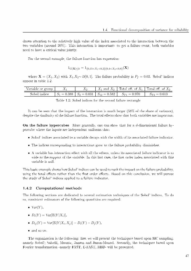
1.4. Fun tional de omposition of varian e for reliability
draws attention to the relatively high value of the index asso iated to the intera tion between the
two variables (around 20%). This intera tion is important: to get a failure event, both variables
need to have a riti al value jointly.
For the se ond example, the failure fun tion has expression:
1G(X)≤k = 10,15<X1<0,20,4<X2<0,8(X)
where X = (X1,X2) with X1,X2∼ U [0, 1]. The failure probability is Pf = 0.02. Sobol' indi es
appear in table 1.2.
Variable or group X1 X2 X1 and X2 Total e. of X1 Total e. of X2
Sobol indi e S1 = 0.388 S2 = 0.031 S12 = 0.582 ST1 = 0.970 ST2 = 0.613
Table 1.2: Sobol indi es for the se ond failure re tangle
It an be seen that the impa t of the intera tion is mu h larger (58% of the share of varian e),
despite the similarity of the failure fun tion. The total ee ts show that both variables are important.
On the failure hyper ubes More generally, one an show that for a d-dimensional failure hy-
per ube where the inputs are independent uniforms that:
Sobol' indi es asso iated to a variable de ays with the width of its asso iated failure indi ator.
The indi es orresponding to intera tions grow as the failure probability diminishes.
A variable has intera tion ee t with all the others, unless its asso iated failure indi ator is as
wide as the support of the variable. In this last ase, the rst order index asso iated with this
variable is null.
This basi example shows how Sobol' indi es an be used to rank the impa t on the failure probability,
using the total ee ts rather than the rst order ee ts. Based on this on lusion, we will pursue
the study of Sobol' indi es applied to a failure indi ator.
1.4.2 Computational methods
The following se tions are dedi ated to several estimation te hniques of the Sobol' indi es. To do
so, onsistent estimators of the following quantities are required:
Var(Y ),
Di(Y ) = Var[E(Y |Xi)],
Dij(Y ) = Var[E(Y |Xi,Xj)]−Di(Y )−Dj(Y ),
and so on.
The organization is the following: rst we will present the te hniques based upon MC sampling,
namely Sobol'; Saltelli, Mauntz, Jansen and Janon-Monod. Se ondly, the te hniques based upon
Fourier transformation -namely FAST, E-FAST, RBD- will be presented.
47
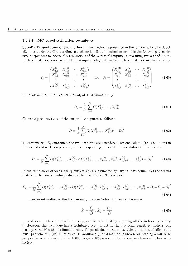
1. State of the art for reliability and sensitivity analysis
1.4.2.1 MC based estimation te hniques
Sobol' - Presentation of the method This method is presented in the founder arti le by Sobol'
[92. Let us denote G the d-dimensional model. Sobol' method prin iple is the following: onsider
two independent matri es of N realisations of the ve tor of d inputs; representing two sets of inputs.
In those matri es, a realisation of the d inputs is gured linewise. Those matri es are the following:
ξ1 =
X(1)1,1 X
(1)1,2 · · · X
(1)1,d
X(1)2,1 X
(1)2,2 · · · X
(1)2,d
.
.
.
.
.
.
.
.
.
.
.
.
X(1)N,1 X
(1)N,2 · · · X
(1)N,2
and ξ2 =
X(2)1,1 X
(2)1,2 · · · X
(2)1,d
X(2)2,1 X
(2)2,2 · · · X
(2)2,d
.
.
.
.
.
.
.
.
.
.
.
.
X(2)N,1 X
(2)N,2 · · · X
(2)N,2
(1.60)
In Sobol' method, the mean of the output Y is estimated by:
D0 =1
N
N∑
k=1
G(X(1)k,1 , . . . ,X
(1)k,d) (1.61)
Conversely, the varian e of the output is omputed as follows:
D =1
N
N∑
k=1
G(X(1)k,1 , . . . ,X
(1)k,d)
2 − D02
(1.62)
To ompute the Di quantities, the two data sets are onsidered, yet one olumn (i.e. i-th input) in
the se ond data-set is repla ed by the orresponding values of the rst data-set. This writes:
Di =1
N
N∑
k=1
G(X(1)k,1 , . . . ,X
(1)k,d)×G(X
(2)k,1 , . . . ,X
(2)k,i−1,X
(1)k,i ,X
(2)k,i+1 . . . ,X
(2)k,d)− D0
2(1.63)
In the same order of ideas, the quantities Dij are estimated by "xing" two olumns of the se ond
matrix to the orresponding values of the rst matrix. This writes:
Dij =1
N
N∑
k=1
G(X(1)k,1 , . . . ,X
(1)k,d)×G(X
(2)k,1 , . . . ,X
(1)k,i ,X
(2)k,i+1 . . . X
(1)k,j ,X
(2)k,j+1 . . . ,X
(2)k,d)− Di− Dj− D0
2
(1.64)
Thus an estimation of the rst, se ond,. . . order Sobol' indi es an be made:
Si =Di
D, Sij =
Dij
D(1.65)
and so on. Thus the total indi es STi an be estimated by summing all the indi es ontaining
i. However, this te hnique has a prohibitive ost: to get all the rst order sensitivity indi es, one
must perform N × (d+1) fun tion alls. To get all the indi es (thus estimate the total indi es) one
must perform N × (2d) fun tion alls. Additionally, this method is known for needing a fair N to
get pre ise estimations, of order 10000 to get a 10% error on the indi es, mu h more for low value
indi es.
48
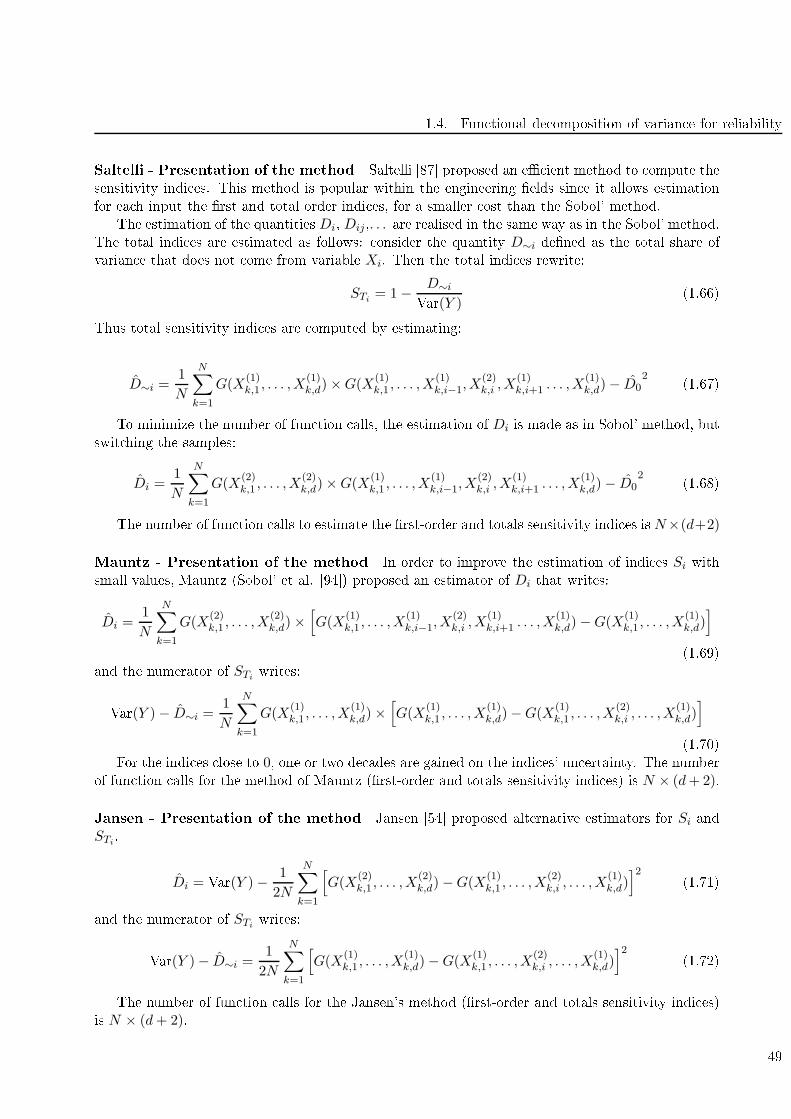
1.4. Fun tional de omposition of varian e for reliability
Saltelli - Presentation of the method Saltelli [87 proposed an e ient method to ompute the
sensitivity indi es. This method is popular within the engineering elds sin e it allows estimation
for ea h input the rst and total order indi es, for a smaller ost than the Sobol' method.
The estimation of the quantities Di, Dij ,. . . are realised in the same way as in the Sobol' method.
The total indi es are estimated as follows: onsider the quantity D∼i dened as the total share of
varian e that does not ome from variable Xi. Then the total indi es rewrite:
STi= 1− D∼i
Var(Y )(1.66)
Thus total sensitivity indi es are omputed by estimating:
D∼i =1
N
N∑
k=1
G(X(1)k,1 , . . . ,X
(1)k,d)×G(X
(1)k,1 , . . . ,X
(1)k,i−1,X
(2)k,i ,X
(1)k,i+1 . . . ,X
(1)k,d)− D0
2(1.67)
To minimize the number of fun tion alls, the estimation of Di is made as in Sobol' method, but
swit hing the samples:
Di =1
N
N∑
k=1
G(X(2)k,1 , . . . ,X
(2)k,d)×G(X
(1)k,1 , . . . ,X
(1)k,i−1,X
(2)k,i ,X
(1)k,i+1 . . . ,X
(1)k,d)− D0
2(1.68)
The number of fun tion alls to estimate the rst-order and totals sensitivity indi es is N×(d+2)
Mauntz - Presentation of the method In order to improve the estimation of indi es Si withsmall values, Mauntz (Sobol' et al. [94) proposed an estimator of Di that writes:
Di =1
N
N∑
k=1
G(X(2)k,1 , . . . ,X
(2)k,d)×
[G(X
(1)k,1 , . . . ,X
(1)k,i−1,X
(2)k,i ,X
(1)k,i+1 . . . ,X
(1)k,d)−G(X
(1)k,1 , . . . ,X
(1)k,d)]
(1.69)
and the numerator of STiwrites:
Var(Y )− D∼i =1
N
N∑
k=1
G(X(1)k,1 , . . . ,X
(1)k,d)×
[G(X
(1)k,1 , . . . ,X
(1)k,d)−G(X
(1)k,1 , . . . ,X
(2)k,i , . . . ,X
(1)k,d)]
(1.70)
For the indi es lose to 0, one or two de ades are gained on the indi es' un ertainty. The number
of fun tion alls for the method of Mauntz (rst-order and totals sensitivity indi es) is N × (d+ 2).
Jansen - Presentation of the method Jansen [54 proposed alternative estimators for Si andSTi
.
Di = Var(Y )− 1
2N
N∑
k=1
[G(X
(2)k,1 , . . . ,X
(2)k,d)−G(X
(1)k,1 , . . . ,X
(2)k,i , . . . ,X
(1)k,d)]2
(1.71)
and the numerator of STiwrites:
Var(Y )− D∼i =1
2N
N∑
k=1
[G(X
(1)k,1 , . . . ,X
(1)k,d)−G(X
(1)k,1 , . . . ,X
(2)k,i , . . . ,X
(1)k,d)]2
(1.72)
The number of fun tion alls for the Jansen's method (rst-order and totals sensitivity indi es)
is N × (d+ 2).
49
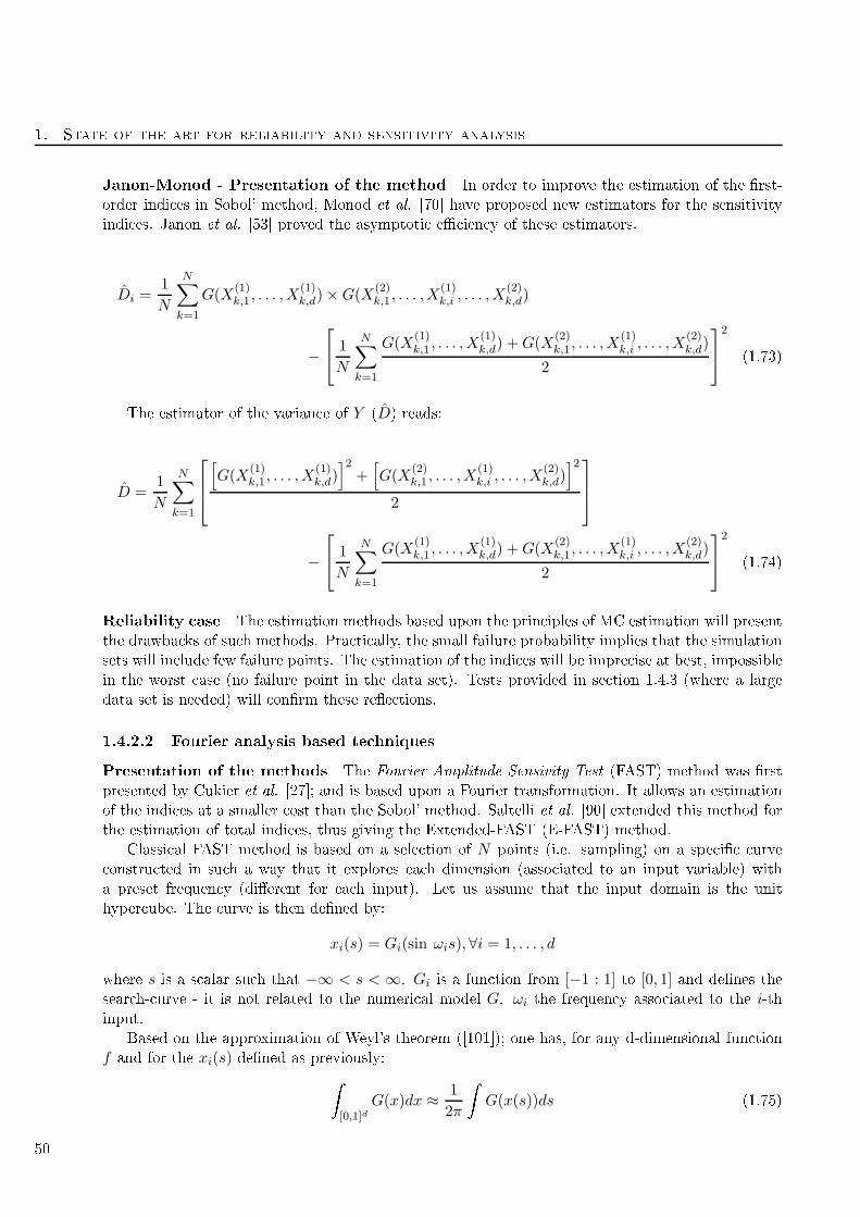
1. State of the art for reliability and sensitivity analysis
Janon-Monod - Presentation of the method In order to improve the estimation of the rst-
order indi es in Sobol' method, Monod et al. [70 have proposed new estimators for the sensitivity
indi es. Janon et al. [53 proved the asymptoti e ien y of these estimators.
Di =1
N
N∑
k=1
G(X(1)k,1 , . . . ,X
(1)k,d)×G(X
(2)k,1 , . . . ,X
(1)k,i , . . . ,X
(2)k,d)
−
1
N
N∑
k=1
G(X(1)k,1 , . . . ,X
(1)k,d) +G(X
(2)k,1 , . . . ,X
(1)k,i , . . . ,X
(2)k,d)
2
2
(1.73)
The estimator of the varian e of Y (D) reads:
D =1
N
N∑
k=1
[G(X
(1)k,1 , . . . ,X
(1)k,d)]2
+[G(X
(2)k,1 , . . . ,X
(1)k,i , . . . ,X
(2)k,d)]2
2
−
1
N
N∑
k=1
G(X(1)k,1 , . . . ,X
(1)k,d) +G(X
(2)k,1 , . . . ,X
(1)k,i , . . . ,X
(2)k,d)
2
2
(1.74)
Reliability ase The estimation methods based upon the prin iples of MC estimation will present
the drawba ks of su h methods. Pra ti ally, the small failure probability implies that the simulation
sets will in lude few failure points. The estimation of the indi es will be impre ise at best, impossible
in the worst ase (no failure point in the data set). Tests provided in se tion 1.4.3 (where a large
data set is needed) will onrm these ree tions.
1.4.2.2 Fourier analysis based te hniques
Presentation of the methods The Fourier Amplitude Sensivity Test (FAST) method was rst
presented by Cukier et al. [27; and is based upon a Fourier transformation. It allows an estimation
of the indi es at a smaller ost than the Sobol' method. Saltelli et al. [90 extended this method for
the estimation of total indi es, thus giving the Extended-FAST (E-FAST) method.
Classi al FAST method is based on a sele tion of N points (i.e. sampling) on a spe i urve
onstru ted in su h a way that it explores ea h dimension (asso iated to an input variable) with
a preset frequen y (dierent for ea h input). Let us assume that the input domain is the unit
hyper ube. The urve is then dened by:
xi(s) = Gi(sin ωis),∀i = 1, . . . , d
where s is a s alar su h that −∞ < s < ∞. Gi is a fun tion from [−1 : 1] to [0, 1] and denes the
sear h- urve - it is not related to the numeri al model G. ωi the frequen y asso iated to the i-thinput.
Based on the approximation of Weyl's theorem ([101); one has, for any d-dimensional fun tion
f and for the xi(s) dened as previously:
[0,1]dG(x)dx ≈ 1
2π
G(x(s))ds (1.75)
50

1.4. Fun tional de omposition of varian e for reliability
where x(s) = (x1(s), . . . , xd(s)). Equation (1.75) is only true when the frequen ies are linearly
independent. This annot be the ase in pra ti e. Therefore the algorithm requires that the pra -
titioner sets a maximal intera tion order M and sele ts the frequen ies free of interferen es up to
M .
The fun tion is then omputed on ea h of theN points, then a Fourier de omposition is performed
on the sample to estimate its spe trum. De omposing the spe trum with respe t to the frequen ies
allows to estimate the estimators of the parts of varian e. Indeed, denoting Aj and Bj the following
Fourier oe ients:
Aj =1
2π
π
−πG(x(s)) cos(js)ds
Bj =1
2π
π
−πG(x(s)) sin(js)ds
Main results from Cu kier et al. [27 is that
Var[Y ] ≈ 2
+∞∑
k=1
(A2k +B2
k) (1.76)
Di = Var[E(Y/Xi)] ≈ 2+∞∑
k=1
(A2kωi
+B2kωi
) (1.77)
The omplexity of su h an algorithm omes from the way to generate the sampling urve, that needs
to explore ea h dimension with preset frequen ies avoiding intera tions.
Random Balan e Design (RBD) method, proposed by Tarantola et al. [96 is a modi ation of
the FAST te hnique. The algorithm starts exploring the input spa e via a sear h urve, but unlike
in FAST, ea h dimension is explored with the same frequen y. Then a random permutation of the
oordinates of the sample points is performed. The fun tion is alled on ea h point of the new
sample, then the Fourier de omposition is arried out for the sampling frequen y and its harmoni s,
up to order M of supposed maximal intera tion order. This allows an estimation of the indi es
asso iated to ea h input. Tissot et al. [97 proposed a way to orre t the biais produ ed in su h
estimates.
Reliability ase It an be expe ted that the FAST/E-FAST/RBD methods will not perform well
in the reliability ase. Indeed, the indi es annot be omputed easily on a dis ontinuous fun tion,
espe ially on the indi ator of a small set. Numeri al tests have shown that a orre t estimation of
the indi es for a dis ontinuous fun tion is possible, provided a high maximal intera tion order M is
sele ted. Unfortunately, in reasing this order leads to frequen y sele tion problems. Therefore the
FAST and derived methods will not be tested in the following.
1.4.3 Reliability test ases
This appli ative subse tion have the following obje tives:
The rst obje tive is to he k the onsisten y of the estimators, to verify that the estimator
of the indi es onverges to the true value as the sample size growths. This will be performed
on test ases for whi h one an easily ompute or approximate losely the indi es.
Another obje tive is to perform the sensitivity analysis on the numeri al examples dened in
Appendix B.
51
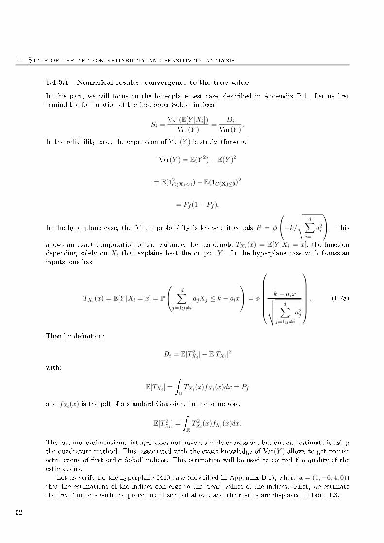
1. State of the art for reliability and sensitivity analysis
1.4.3.1 Numeri al results: onvergen e to the true value
In this part, we will fo us on the hyperplane test ase, des ribed in Appendix B.1. Let us rst
remind the formulation of the rst order Sobol' indi es:
Si =Var(E[Y |Xi])
Var(Y )=
Di
Var(Y ).
In the reliability ase, the expression of Var(Y ) is straightforward:
Var(Y ) = E(Y 2)− E(Y )2
= E(12G(X)≤0)− E(1G(X)≤0)2
= Pf (1− Pf ).
In the hyperplane ase, the failure probability is known: it equals P = φ
−k/
√√√√d∑
i=1
a2i
. This
allows an exa t omputation of the varian e. Let us denote TXi(x) = E[Y |Xi = x], the fun tion
depending solely on Xi that explains best the output Y . In the hyperplane ase with Gaussian
inputs, one has:
TXi(x) = E[Y |Xi = x] = P
d∑
j=1;j 6=i
ajXj ≤ k − aix
= φ
k − aix√√√√d∑
j=1;j 6=i
a2j
. (1.78)
Then by denition:
Di = E[T 2Xi]− E[TXi
]2
with:
E[TXi] =
R
TXi(x)fXi
(x)dx = Pf
and fXi(x) is the pdf of a standard Gaussian. In the same way,
E[T 2Xi] =
R
T 2Xi(x)fXi
(x)dx.
The last mono-dimensional integral does not have a simple expression, but one an estimate it using
the quadrature method. This, asso iated with the exa t knowledge of Var(Y ) allows to get pre ise
estimations of rst order Sobol' indi es. This estimation will be used to ontrol the quality of the
estimations.
Let us verify for the hyperplane 6410 ase (des ribed in Appendix B.1), where a = (1,−6, 4, 0))that the estimations of the indi es onverge to the real values of the indi es. First, we estimate
the real indi es with the pro edure des ribed above, and the results are displayed in table 1.3.
52

1.4. Fun tional de omposition of varian e for reliability
Variable X1 X2 X3 X4
Indi e Si 0.002 0.259 0.055 0
Table 1.3: First order Sobol' indi es for the hyperplane 6410 ase
104 105 106
−0.
010.
000.
010.
020.
03
estim
atio
n of
S1
104 105 106
0.15
0.20
0.25
0.30
0.35
estim
atio
n of
S2
104 105 106
0.00
0.04
0.08
0.12
estim
atio
n of
S3
104 105 106
−0.
010.
000.
010.
020.
03
estim
atio
n of
S4
Figure 1.5: Boxplots of the estimated rst order Sobol' indi es with the Sobol' method
We repeat the following operation 500 times: generating two samples of size N , with N varying
from 104 to 106, and estimating the indi es on all these samples. The results of the estimation of
the rst order Sobol' indi es are shown in gure 1.5 for the Sobol' method and in gure 1.6 for the
Saltelli method.
The graphi s show that the estimator onverges to the true value when the sample size in reases.
Additionally, it shows that the estimations of a null index (S4) with the Sobol' method an provide
results with a wider spread than the ones provided with the Saltelli method. For this reason, we will
use the Saltelli method in the following. Con erning the good sample size to orre tly estimate the
Sobol' indi es, the results show that obviously the larger the sample is, the better the estimation is.
For our test ases, we will use samples of size 106, sin e our toy-models are not ostly. However it
should be noti ed that this number of fun tion alls might be unrealisti for real models.
1.4.3.2 Hyperplane 6410 ase
We present on table 1.4 the estimated Sobol' indi es with 2 samples of size 106, using the Saltelli
method. The total number of fun tion evaluations is 6× 10⁶.
Index S1 S2 S3 S4 ST1 ST2 ST3 ST4
Estimation 0.002 0.254 0.054 0 0.200 0.940 0.720 0
Table 1.4: Estimated Sobol' indi es for the hyperplane 6410 ase
53
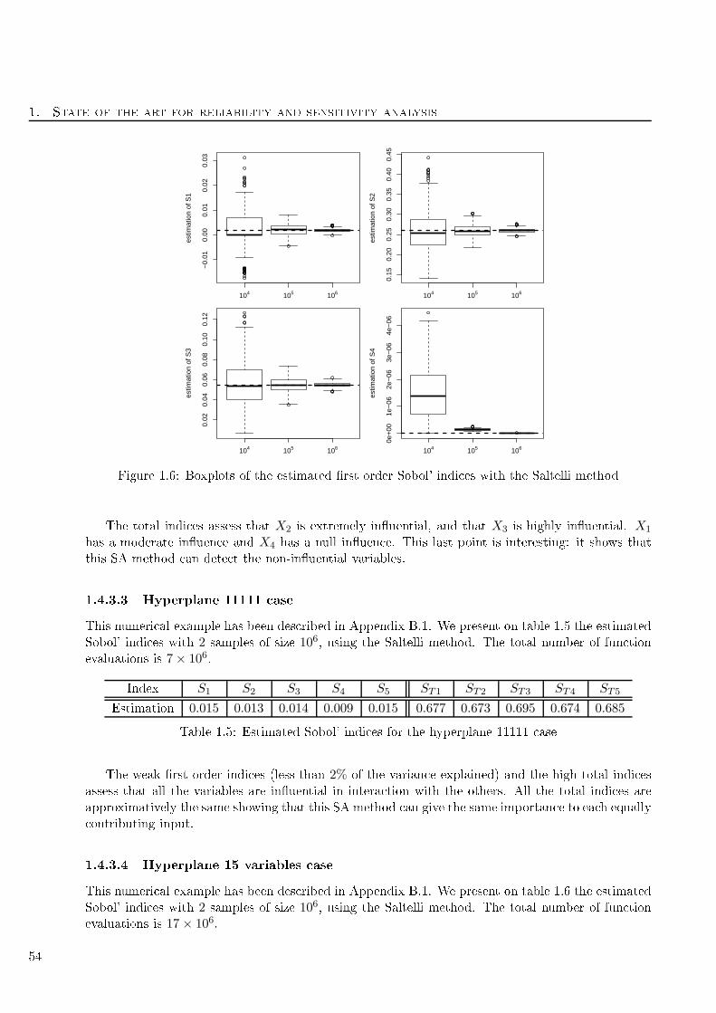
1. State of the art for reliability and sensitivity analysis
104 105 106
−0.
010.
000.
010.
020.
03
estim
atio
n of
S1
104 105 106
0.15
0.20
0.25
0.30
0.35
0.40
0.45
estim
atio
n of
S2
104 105 106
0.02
0.04
0.06
0.08
0.10
0.12
estim
atio
n of
S3
104 105 106
0e+
001e
−06
2e−
063e
−06
4e−
06
estim
atio
n of
S4
Figure 1.6: Boxplots of the estimated rst order Sobol' indi es with the Saltelli method
The total indi es assess that X2 is extremely inuential, and that X3 is highly inuential. X1
has a moderate inuen e and X4 has a null inuen e. This last point is interesting: it shows that
this SA method an dete t the non-inuential variables.
1.4.3.3 Hyperplane 11111 ase
This numeri al example has been des ribed in Appendix B.1. We present on table 1.5 the estimated
Sobol' indi es with 2 samples of size 106, using the Saltelli method. The total number of fun tion
evaluations is 7× 10⁶.
Index S1 S2 S3 S4 S5 ST1 ST2 ST3 ST4 ST5
Estimation 0.015 0.013 0.014 0.009 0.015 0.677 0.673 0.695 0.674 0.685
Table 1.5: Estimated Sobol' indi es for the hyperplane 11111 ase
The weak rst order indi es (less than 2% of the varian e explained) and the high total indi es
assess that all the variables are inuential in intera tion with the others. All the total indi es are
approximatively the same showing that this SA method an give the same importan e to ea h equally
ontributing input.
1.4.3.4 Hyperplane 15 variables ase
This numeri al example has been des ribed in Appendix B.1. We present on table 1.6 the estimated
Sobol' indi es with 2 samples of size 106, using the Saltelli method. The total number of fun tion
evaluations is 17× 106.
54
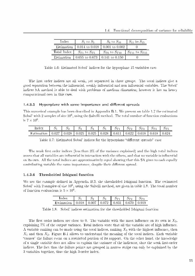
1.4. Fun tional de omposition of varian e for reliability
Index S1 to S5 S6 to S10 S11 to S15
Estimation 0.014 to 0.018 0.001 to 0.002 0
Total Index ST1 to ST5 ST6 to ST10 ST11 to ST15
Estimation 0.655 to 0.673 0.141 to 0.150 0
Table 1.6: Estimated Sobol' indi es for the hyperplane 15 variables ase
The rst order indi es are all weak, yet separated in three groups. The total indi es give a
good separation between the inuential, weakly inuential and non inuential variables. The Sobol'
indi es SA method is able to deal with problems of medium dimension; however it has an heavy
omputational ost in this ase.
1.4.3.5 Hyperplane with same importan e and dierent spreads
This numeri al example has been des ribed in Appendix B.1. We present on table 1.7 the estimated
Sobol' with 2 samples of size 106, using the Saltelli method. The total number of fun tion evaluations
is 7× 10⁶.
Index S1 S2 S3 S4 S5 ST1 ST2 ST3 ST4 ST5
Estimation 0.027 0.028 0.025 0.025 0.028 0.611 0.622 0.618 0.618 0.624
Table 1.7: Estimated Sobol' indi es for the hyperplane dierent spreads ase
The weak rst order indi es (less than 3% of the varian e explained) and the high total indi es
assess that all variables are inuential in intera tion with the others, and that no variable is inuential
on its own. All the total indi es are approximatively equal showing that this SA gives to ea h equally
ontributing variable the same importan e, despite their dierent spread.
1.4.3.6 Thresholded Ishigami fun tion
We use the example dened in Appendix B.2, the thresholded Ishigami fun tion. The estimated
Sobol' with 2 samples of size 106, using the Saltelli method, are given in table 1.8. The total number
of fun tion evaluations is 5× 10⁶.
Index S1 S2 S3 ST1 ST2 ST3
Estimation 0.018 0.007 0.072 0.831 0.670 0.919
Table 1.8: Sobol' indi es estimation for the thresholded Ishigami fun tion
The rst order indi es are lose to 0. The variable with the most inuen e on its own is X3,
explaining 7% of the output varian e. Total indi es state that all the variable are of high inuen e.
A variable ranking an be made using the total indi es, ranking X3 with the highest inuen e, then
X1 and then X2. Figure B.1 allows to understand the meaning of the total indi es. Ea h variable
auses the failure event on a restri ted portion of its support. On the other hand, the knowledge
of a single variable does not allow to explain the varian e of the indi ator, thus the weak rst-order
indi es. The fa t that the failure points are grouped in narrow strips an only be explained by the
3 variables together, thus the high 3-order index.
55

1. State of the art for reliability and sensitivity analysis
1.4.3.7 Flood ase
This test ase has been des ribed in Appendix B.3. The estimated Sobol' with 2 samples of size
106, using the Saltelli method, are given in table 1.9. The total number of fun tion evaluations is
6× 10⁶.
Index SQ SKs SZv SZm STQ STKs STZv STZm
Estimation 0.019 0.251 0 0 0.746 0.976 0.248 0.115
Table 1.9: Estimated Sobol' indi es for the ood ase
Most rst order indi es are small, ex ept the one asso iated to Ks that explains 25% of the
varian e on its own. The total indi es state that Ks and Q are extremely inuential, Zv is inuential
and Zm is little inuential. One an see that STZv and STZm dier from 0, meaning these variables
have an impa t on the failure probability when intera ting with other variables.
1.4.3.8 Con lusion
In most tested ases, Sobol' indi es allow distinguishing the inuential and the non-inuential vari-
ables. However, their evaluation is ostly. The obje tive of the two next subse tions is to study
methods that allow a redu tion of fun tion alls.
1.4.4 Redu ing the number of fun tion alls: use of QMC methods
This subse tion fo uses on the use of Quasi Monte-Carlo methods (presented in se tion 1.2.1.2) to
estimate Sobol' indi es. This te hnique is presented in Sobol' [93.
1.4.4.1 Estimation of Sobol' indi es through QMC
The main idea when using pseudo-random sequen es is to use the estimators presented in se tion
1.4.2.1, repla ing the random samples by samples oming from a low-dis repan y sequen e. In the
following, Sobol' sequen e is used (see Niederreiter [75).
When estimating the indi es with the Sobol' method, 2 samples of size N and of dimension di.i.d. to X are generated. These samples are then separated in omplementary sets. A generation of
two samples from the pseudo-random sequen e is meaningless, sin e it is a deterministi sequen e.
The tri k is to generate a sample of size N and of dimension 2d, then to split this sample. Su h a
separation allows to get two samples of dimension d. Sobol' sequen e produ es orthogonal olumns,
these pseudo-random samples an be onsidered as independent. As an example on the pseudo-
random sample generation, table 1.10 displays the 8 rst points generated by Sobol' sequen e in
dimension 4.
1.4.4.2 Illustration on the hyperplane test ase
In this part, the fo us will be set on the hyperplane 6410 test ase, des ribed in Appendix B.1. The
aim of this part is to assess the apability of QMC sampling to get a good estimation of Sobol'
indi es at a smaller omputational ost.
First, two QMC samples of size 104 and of dimension 4 are generated (using the tri k given
above). The same is done for size 105. Let us noti e that the sample of size 104 is in luded in the
one of size 105, due to the determinism of the Sobol' sequen e. Then the Sobol' indi es are estimated
56
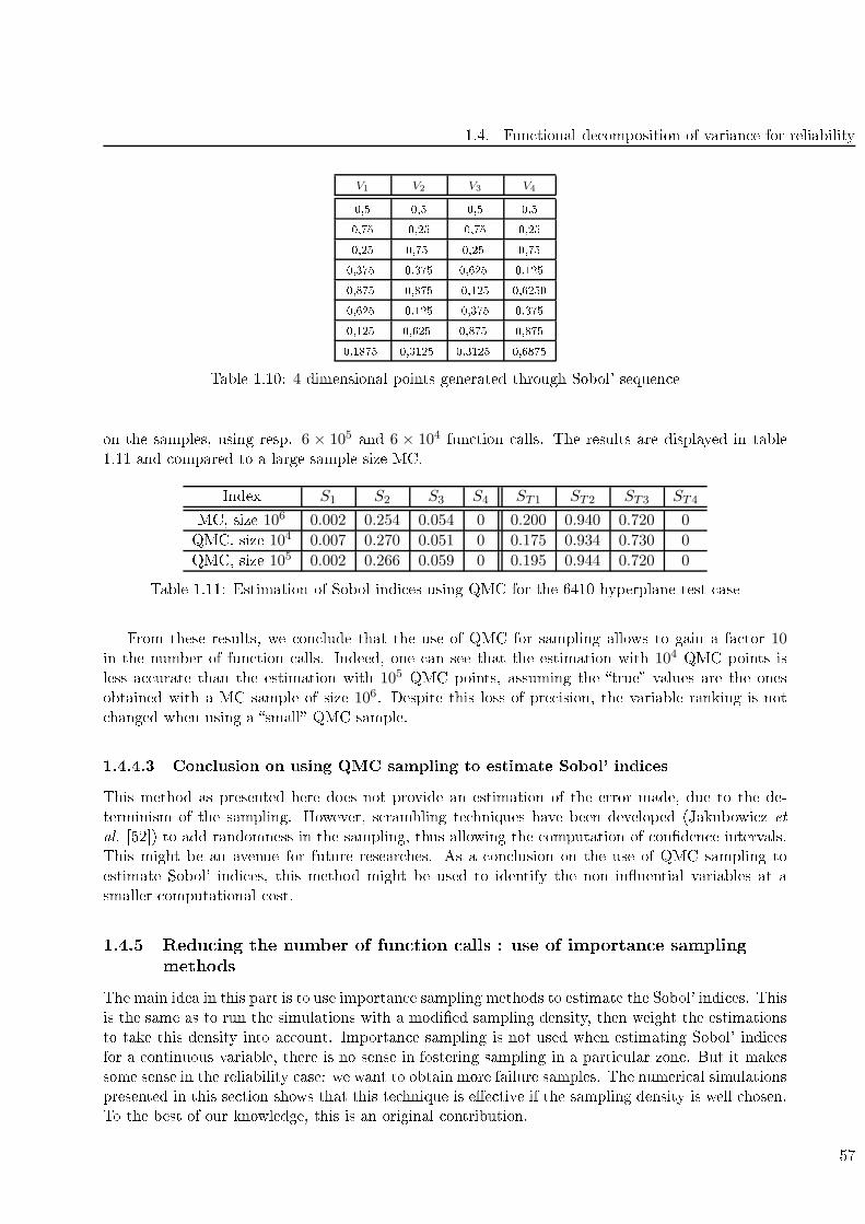
1.4. Fun tional de omposition of varian e for reliability
V1 V2 V3 V4
0,5 0,5 0,5 0,5
0,75 0,25 0,75 0,25
0,25 0,75 0,25 0,75
0,375 0,375 0,625 0,125
0,875 0,875 0,125 0,6250
0,625 0,125 0,375 0,375
0,125 0,625 0,875 0,875
0,1875 0,3125 0,3125 0,6875
Table 1.10: 4 dimensional points generated through Sobol' sequen e
on the samples, using resp. 6 × 10⁵ and 6 × 10⁴ fun tion alls. The results are displayed in table
1.11 and ompared to a large sample size MC.
Index S1 S2 S3 S4 ST1 ST2 ST3 ST4
MC, size 106 0.002 0.254 0.054 0 0.200 0.940 0.720 0
QMC, size 104 0.007 0.270 0.051 0 0.175 0.934 0.730 0
QMC, size 105 0.002 0.266 0.059 0 0.195 0.944 0.720 0
Table 1.11: Estimation of Sobol indi es using QMC for the 6410 hyperplane test ase
From these results, we on lude that the use of QMC for sampling allows to gain a fa tor 10in the number of fun tion alls. Indeed, one an see that the estimation with 104 QMC points is
less a urate than the estimation with 105 QMC points, assuming the true values are the ones
obtained with a MC sample of size 106. Despite this loss of pre ision, the variable ranking is not
hanged when using a small QMC sample.
1.4.4.3 Con lusion on using QMC sampling to estimate Sobol' indi es
This method as presented here does not provide an estimation of the error made, due to the de-
terminism of the sampling. However, s rambling te hniques have been developed (Jakubowi z et
al. [52) to add randomness in the sampling, thus allowing the omputation of onden e intervals.
This might be an avenue for future resear hes. As a on lusion on the use of QMC sampling to
estimate Sobol' indi es, this method might be used to identify the non inuential variables at a
smaller omputational ost.
1.4.5 Redu ing the number of fun tion alls : use of importan e sampling
methods
The main idea in this part is to use importan e sampling methods to estimate the Sobol' indi es. This
is the same as to run the simulations with a modied sampling density, then weight the estimations
to take this density into a ount. Importan e sampling is not used when estimating Sobol' indi es
for a ontinuous variable, there is no sense in fostering sampling in a parti ular zone. But it makes
some sense in the reliability ase: we want to obtain more failure samples. The numeri al simulations
presented in this se tion shows that this te hnique is ee tive if the sampling density is well hosen.
To the best of our knowledge, this is an original ontribution.
57
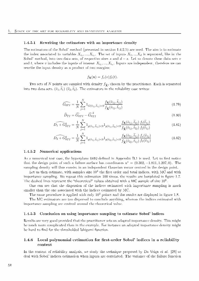
1. State of the art for reliability and sensitivity analysis
1.4.5.1 Rewriting the estimators with an importan e density
The estimators of the Sobol' method (presented in se tion 1.4.2.1) are used. The aim is to estimate
the index asso iated to variables Xi1 , ...,Xis . The set of inputs X1, ..,Xd is separated, like in the
Sobol' method, into two data sets, of respe tive sizes s and d − s. Let us denote these data sets vand t, where v in ludes the inputs of interest Xi1 , ...,Xis . Inputs are independent, therefore we an
rewrite the input density as a produ t of two margins:
fX(x) = fv(v)ft(t).
Two sets of N points are sampled with density fX, hosen by the pra titioner. Ea h is separated
into two data sets, (v1, t1) (v2, t2). The estimators in the reliability ase writes:
G0TI =1
N
N∑
j=1
1G(v1j ,t1j)<0
fX(v1j , t1j)
fX(v1j , t1j)
(1.79)
DTI = G0TI − G02
TI (1.80)
D1 +G20TI =
1
N
N∑
j=1
1g(v1j ,t1j)<01g(v1j ,t2j)<0
fX(v1j , t2j)
fX(v1j , t2j)
ft(t1j)
ft(t1j)(1.81)
D2 +G20TI =
1
N
N∑
j=1
1g(v1j ,t1j)<01g(v2j ,t1j)<0
fX(v2j , t1j)
fX(v2j , t1j)
fv(v1j)
fv(v1j)(1.82)
1.4.5.2 Numeri al appli ations
As a numeri al test ase, the hyperplane 6410 dened in Appendix B.1 is used. Let us rst noti e
that the design point of su h a failure surfa e has oordinates u∗ = (0.302,−1.811, 1.207, 0). The
sampling density will thus onsist in an independent Gaussian ve tor entred in the design point.
Let us then estimate, with samples size 104 the rst order and total indi es, with MC and with
importan e sampling. We repeat this estimation 100 times, the results are boxploted in gure 1.7.
The dashed lines represent the theoreti al values obtained with a MC sample of size 106.
One an see that the dispersion of the indi es estimated with importan e sampling is mu h
smaller than the one asso iated with the indi es estimated by MC.
The same pro edure is applied with only 103 points and the results are displayed in gure 1.8.
The MC estimators are too dispersed to on lude anything, whereas the indi es estimated with
importan e sampling are entred around the theoreti al value.
1.4.5.3 Con lusion on using importan e sampling to estimate Sobol' indi es
Results are very good provided that the pra titioner sets an adapted importan e density. This might
be mu h more ompli ated than in the example. For instan e an adapted importan e density might
be hard to nd for the thresholded Ishigami fun tion.
1.4.6 Lo al polynomial estimation for rst-order Sobol' indi es in a reliability
ontext
In the ontext of reliability analysis, we study the te hnique proposed by Da Veiga et al. [28 to
deal with Sobol' indi es estimation when inputs are orrelated. The varian e of the failure fun tion
58

1.4. Fun tional de omposition of varian e for reliability
S1 S3 ST1 ST3
0.0
0.2
0.4
0.6
0.8
1.0
Est
imat
ions
S1 S3 ST1 ST3
0.0
0.2
0.4
0.6
0.8
Est
imat
ions
Figure 1.7: Comparison of rst order and total indi es, MC (left) and importan e sampling (right),
with 104 points for the hyperplane 6410 test ase
within the failure domain is of interest here. The presented method is used to nd out the rst-order
ontribution of ea h variable to this varian e. The question asked in this subse tion is How ea h
variable ontributes to the varian e of the failure fun tion G within the failure domain? .
1.4.6.1 Sobol' indi es estimation by lo al polynomial smoothing
Let us re all that for a mathemati al model denoted G : Rd → R with random inputs X ∼ f and
random output Y , rst order Sobol' indi es are given by:
Sk =Var
(E(Y/Xk
))
Var (Y ), ∀k = 1, . . . , d. (1.83)
In the ase of independent inputs, one an quote Sobol' and FAST estimation te hniques, as presented
in se tion 1.4.2. These methods annot be applied when the inputs are no longer independent.
Nevertheless there is a need for sensitivity analysis methods when inputs are non-independently
distributed. Several re ent works deal with this kind of problems.
59

1. State of the art for reliability and sensitivity analysis
S1 S3 ST1 ST3
0.0
0.2
0.4
0.6
0.8
1.0
Est
imat
ions
S1 S3 ST1 ST3
0.0
0.2
0.4
0.6
0.8
Est
imat
ions
Figure 1.8: Comparison of rst order and total indi es, MC (left) and importan e sampling (right),
with 103 points for the hyperplane 6410 test ase
The original te hnique proposed by Da Veiga et al. [28 to estimate Sk is based on lo al poly-
nomial approximation of the onditional moments. More pre isely the authors use a rst sample
(Xi, Yi)i=1,...,N to t d lo al polynomial response surfa e to explain the following relationship for
ea h given input k:
Yi = mk(Xki ) + σk(X
ki )ǫ
ki (1.84)
where mk(x) = E(Y/Xk = x
)and σ2k(x) = Var
(Y/Xk = x
)(x ∈ R). ǫki ∀i = 1, . . . , N are indepen-
dent errors satisfying E(ǫki /X
k)= 0 and Var
(ǫki /X
k)= 1. The lo al polynomial (LP) smoothing
provides estimators for mk(.) and σ2k(.). Two formulations for Sobol' rst order indi es are given in
the arti le, we hoose to fo us on the one involving mk(.). Given another sample of i.i.d. inputs(Xi
)i=1,...,N ′
with same distribution as X, one an use a plug-in estimation as follow. Denoting
m(.) the LP estimator of the onditional expe tation, tted on the rst sample; denoting as well
60
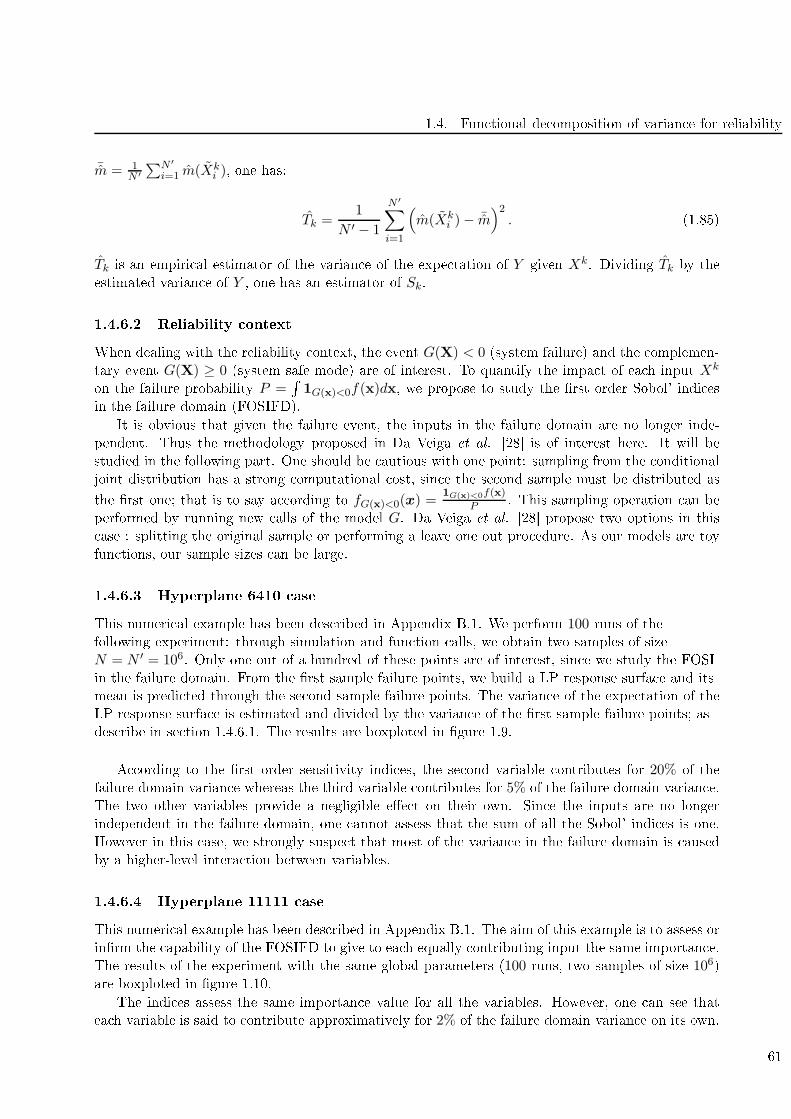
1.4. Fun tional de omposition of varian e for reliability
¯m = 1N ′
∑N ′
i=1 m(Xki ), one has:
Tk =1
N ′ − 1
N ′∑
i=1
(m(Xk
i )− ¯m)2. (1.85)
Tk is an empiri al estimator of the varian e of the expe tation of Y given Xk. Dividing Tk by the
estimated varian e of Y , one has an estimator of Sk.
1.4.6.2 Reliability ontext
When dealing with the reliability ontext, the event G(X) < 0 (system failure) and the omplemen-
tary event G(X) ≥ 0 (system safe mode) are of interest. To quantify the impa t of ea h input Xk
on the failure probability P =
1G(x)<0f(x)dx, we propose to study the rst order Sobol' indi es
in the failure domain (FOSIFD).
It is obvious that given the failure event, the inputs in the failure domain are no longer inde-
pendent. Thus the methodology proposed in Da Veiga et al. [28 is of interest here. It will be
studied in the following part. One should be autious with one point: sampling from the onditional
joint distribution has a strong omputational ost, sin e the se ond sample must be distributed as
the rst one; that is to say a ording to fG(x)<0(x) =1G(x)<0f(x)
P . This sampling operation an be
performed by running new alls of the model G. Da Veiga et al. [28 propose two options in this
ase : splitting the original sample or performing a leave one out pro edure. As our models are toy
fun tions, our sample sizes an be large.
1.4.6.3 Hyperplane 6410 ase
This numeri al example has been des ribed in Appendix B.1. We perform 100 runs of the
following experiment: through simulation and fun tion alls, we obtain two samples of size
N = N ′ = 106. Only one out of a hundred of these points are of interest, sin e we study the FOSI
in the failure domain. From the rst sample failure points, we build a LP response surfa e and its
mean is predi ted through the se ond sample failure points. The varian e of the expe tation of the
LP response surfa e is estimated and divided by the varian e of the rst sample failure points; as
des ribe in se tion 1.4.6.1. The results are boxploted in gure 1.9.
A ording to the rst order sensitivity indi es, the se ond variable ontributes for 20% of the
failure domain varian e whereas the third variable ontributes for 5% of the failure domain varian e.
The two other variables provide a negligible ee t on their own. Sin e the inputs are no longer
independent in the failure domain, one annot assess that the sum of all the Sobol' indi es is one.
However in this ase, we strongly suspe t that most of the varian e in the failure domain is aused
by a higher-level intera tion between variables.
1.4.6.4 Hyperplane 11111 ase
This numeri al example has been des ribed in Appendix B.1. The aim of this example is to assess or
inrm the apability of the FOSIFD to give to ea h equally ontributing input the same importan e.
The results of the experiment with the same global parameters (100 runs, two samples of size 106)are boxploted in gure 1.10.
The indi es assess the same importan e value for all the variables. However, one an see that
ea h variable is said to ontribute approximatively for 2% of the failure domain varian e on its own.
61
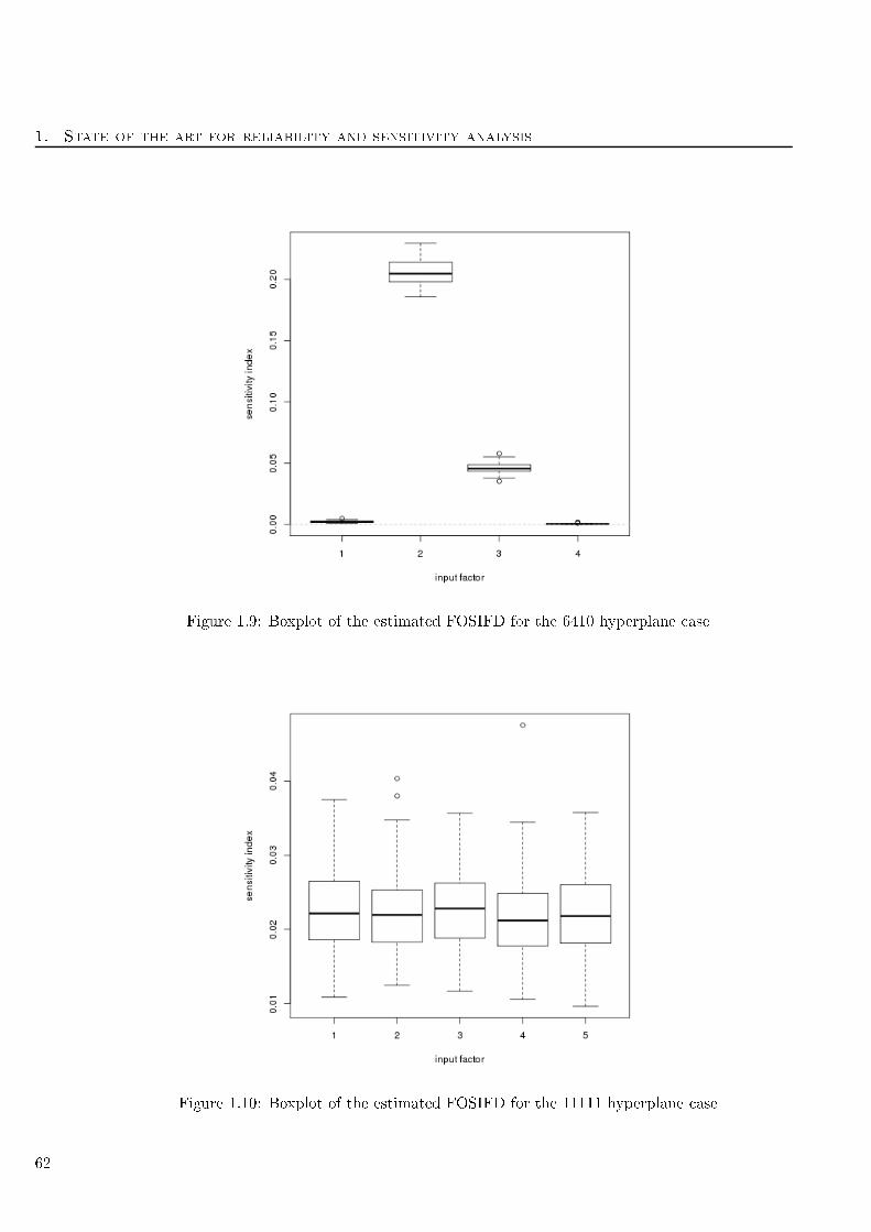
1. State of the art for reliability and sensitivity analysis
Figure 1.9: Boxplot of the estimated FOSIFD for the 6410 hyperplane ase
Figure 1.10: Boxplot of the estimated FOSIFD for the 11111 hyperplane ase
62

1.4. Fun tional de omposition of varian e for reliability
Therefore, as in the previous ase, we suspe t that there is a higher-order intera tion that auses
most of the varian e in the failure domain.
1.4.6.5 Hyperplane 15 variables ase
This numeri al example has been des ribed in Appendix B.1. The results of the experiment with
the same global parameters (100 runs, two samples of size 106) are boxploted in gure 1.11.
Figure 1.11: Boxplot of the estimated FOSIFD for the 15 variables hyperplane ase
As one an see two groups of importan e variables, one an on lude that the FOSIFD fails
to separate variables with a low ontribution and variables with a null ontribution. However,
the inuential variables are dete ted and ontribute for approximatively 2% of the failure domain
varian e.
1.4.6.6 Hyperplane with same importan e and dierent spreads
This numeri al example has been des ribed in Appendix B.1. The aim of this test is to assess or inrm
the apability of the FOSIFD to give to ea h equally ontributing variable the same importan e,
despite their dierent spread. The results of the experiment with the same global parameters (100runs, two samples of size 106) are boxploted in gure 1.12.
One an see that the values of the FOSIFD are approximatively equal for ea h variable. Thus,
ea h variable explain on its own 2% of the failure domain varian e. These results are the same as in
se tion 1.4.6.4. Thus one an think that the spread of the variable has no impa t, at least on this
test ase.
1.4.6.7 Tresholded Ishigami fun tion
This numeri al example has been des ribed in Appendix B.2. The results of the experiment with
the same global parameters (100 runs, two samples of size 106) are boxploted in gure 1.13.
63
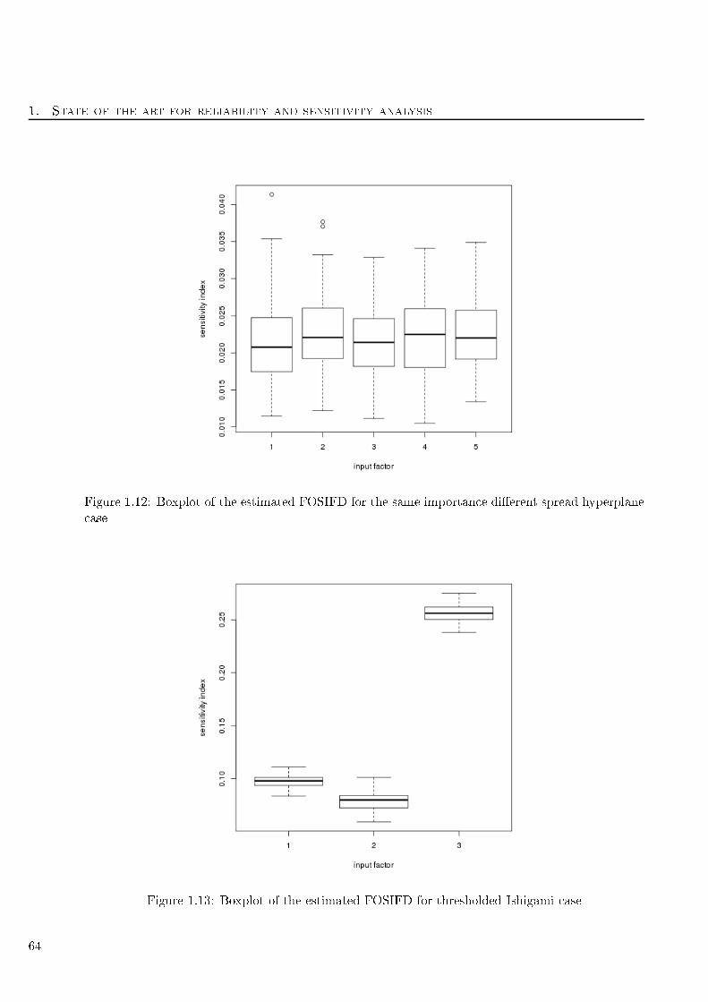
1. State of the art for reliability and sensitivity analysis
Figure 1.12: Boxplot of the estimated FOSIFD for the same importan e dierent spread hyperplane
ase
Figure 1.13: Boxplot of the estimated FOSIFD for thresholded Ishigami ase
64
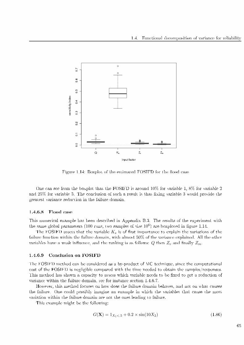
1.4. Fun tional de omposition of varian e for reliability
Figure 1.14: Boxplot of the estimated FOSIFD for the ood ase
One an see from the boxplot that the FOSIFD is around 10% for variable 1, 8% for variable 2
and 25% for variable 3. The on lusion of su h a result is that xing variable 3 would provide the
greatest varian e redu tion in the failure domain.
1.4.6.8 Flood ase
This numeri al example has been des ribed in Appendix B.3. The results of the experiment with
the same global parameters (100 runs, two samples of size 106) are boxploted in gure 1.14.
The FOSIFD assess that the variable Ks is of rst importan e to explain the variations of the
failure fun tion within the failure domain, with almost 50% of the varian e explained. All the other
variables have a weak inuen e, and the ranking is as follows: Q then Zv and nally Zm.
1.4.6.9 Con lusion on FOSIFD
The FOSIFD method an be onsidered as a by-produ t of MC te hnique, sin e the omputational
ost of the FOSIFD is negligible ompared with the time needed to obtain the samples/responses.
This method has shown a apa ity to assess whi h variable needs to be xed to get a redu tion of
varian e within the failure domain, see for instan e se tion 1.4.6.7.
However, this method fo uses on how does the failure domain behaves, and not on what auses
the failure. One ould possibly imagine an example in whi h the variables that ause the most
variation within the failure domain are not the ones leading to failure.
This example might be the following:
G(X) = 1X1<.5 + 0.2 × sin(10X2) (1.86)
65

1. State of the art for reliability and sensitivity analysis
x1x2
G(X)
Figure 1.15: Example surfa e
where X1,X2 ∼ U [0, 1] and the failure event is when G(x) < 0. The surfa e pi turing su h a
fun tion is displayed in Figure 1.15 .
It an be seen that the failure event is only aused by variable X1 whereas the variation within
the failure domain is only aused by variable X2. The Sobol' indi es of the indi ator fun tion are
S1 = 1 and S2 = 0 whereas the FOSIFD worth respe tively 0 and 0.91 for variables X1 and X2.
Consequently, if the obje tive is the varian e redu tion within the failure domain, one should fo us
on variable X2 but if the obje tive is to understand what auses the failure event, one should fo us
on variable X1.
As in our study we are more interested in the failure event, we will not pursue the testing of the
FOSIFD method.
1.4.7 Con lusion on Sobol' indi es for reliability
Sobol' indi es applied dire tly on the indi ator fun tion have shown a apa ity to separate the
inuential and non-inuential variables. Based on this observation, it seems an adapted method for
sensitivity analysis in the reliability ontext. However, in most tested ases, Sobol' indi es behave
as follows: weak rst order indi es, strong total indi es. This assesses that no variable is inuential
on its own, and that most variables ontribute to the failure probability when intera ting with the
others. Unfortunately in most stru tural reliability ases, this is an already known information: it
is when all the variable takes extreme values at the same time that the equipment fails. However,
Sobol' total indi es onvey a strong information if the obje tive is the dis rimination of the inuential
and non-inuential variables.
One an observe that this useful information is obtained at a strong omputational ost. As
a rule of thumb we suggest to use samples of size 106 for failure probabilities of order 10−3: with
smaller sample sizes the estimations might be too noisy. Varian e redu tion te hnique have been
studied, QMC and importan e sampling. QMC allows a redu tion of fun tion alls of order 10.Importan e sampling might be used if the goal of the SA is to rank the variable (i.e. obtain a
qualitative information) and an lead to a redu tion of fun tion alls of order 100. However, su h a
redu tion is possible only if a good importan e density is available.
66

1.5. Moment independent measures for reliability
If the model is not ostly we would re ommend the use of su h indi es, using the Saltelli [87
method that allows an estimation of the rst order and total indi es. Other methods an be quoted
and are ompared in Saltelli et al. [88. However if the model is ostly, other methods than the
Sobol' indi es need to be found.
1.5 Moment independent measures for reliability
Let us study, in the reliability ase, the indi es dened in Borgonovo [13 that have been presented
in se tion 1.3.1.4.
1.5.1 Appli ation in the reliability ase
For the reliability ase, one has:
fY ∼ B(Pf ) with Pf =
1G(x)≤0fX(x)dx (1.87)
where B(p) denotes the Bernoulli distribution of parameter p. When xing the ith output to a given
value xi, one denotes:
fY |Xi=xi∼ B(Pxi
) with Pxi=
1G(x1,...,xi,...,xn)≤0fX−i(x−i)dx−i (1.88)
Then, the shift dened in Equation (1.54) rewrites as follows:
s(xi) =1∑
y=0
|fY (y)− fY |Xi=xi(y)| = |(1 − Pf )− (1− Pxi
)|+ |Pf − Pxi|
= 2|Pf − Pxi|. (1.89)
Thus the sensitivity index dened in Equation (1.56) rewrites:
δi =1
2EXi
[s(Xi)] =
fXi(xi)|Pf − Pxi
|dxi. (1.90)
If the quantities Pf and Pxiare known, this is a one-dimensional integral.
1.5.2 Crude MC estimation of δi
Let us expli it here the methodology to use in order to estimate the indi es δi by rude MC. First
of all, an estimation of Pf is made with N1 points:
P =1
N1
N1∑
j=1
1G(x(j))<0 (1.91)
where x(j), j = 1, . . . , N1 are i.i.d. realisations of fX. Then, for a given xi that lies in the support
of fXi, let us estimate Pxi
with a rude MC:
Pxi=
1
N2
N2∑
j=1
1G(x
(j)−i ,xi)<0
fX−i(x−i) (1.92)
67
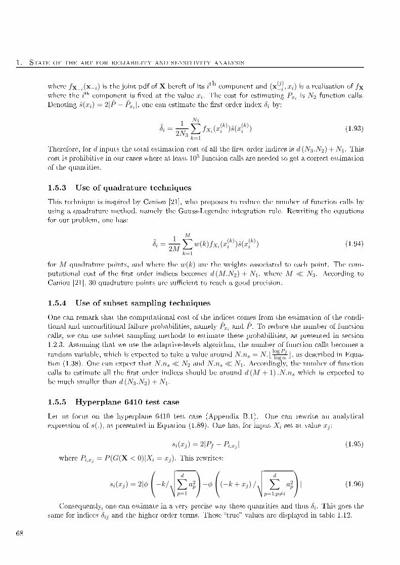
1. State of the art for reliability and sensitivity analysis
where fX−i(x−i) is the joint pdf of X bereft of its ith omponent and (x
(j)−i , xi) is a realisation of fX
where the ith omponent is xed at the value xi. The ost for estimating Pxiis N2 fun tion alls.
Denoting s(xi) = 2|P − Pxi|, one an estimate the rst order index δi by:
δi =1
2N3
N3∑
k=1
fXi(x
(k)i )s(x
(k)i ) (1.93)
Therefore, for d inputs the total estimation ost of all the rst order indi es is d (N3.N2)+N1. This
ost is prohibitive in our ases where at least 105 fun tion alls are needed to get a orre t estimation
of the quantities.
1.5.3 Use of quadrature te hniques
This te hnique is inspired by Caniou [21, who proposes to redu e the number of fun tion alls by
using a quadrature method, namely the Gauss-Legendre integration rule. Rewriting the equations
for our problem, one has:
δi =1
2M
M∑
k=1
w(k)fXi(x
(k)i )s(x
(k)i ) (1.94)
for M quadrature points, and where the w(k) are the weights asso iated to ea h point. The om-
putational ost of the rst order indi es be omes d (M.N2) + N1, where M ≪ N3. A ording to
Caniou [21, 30 quadrature points are su ient to rea h a good pre ision.
1.5.4 Use of subset sampling te hniques
One an remark that the omputational ost of the indi es omes from the estimation of the ondi-
tional and un onditional failure probabilities, namely Pxiand P . To redu e the number of fun tion
alls, we an use subset sampling methods to estimate these probabilities, as presented in se tion
1.2.3. Assuming that we use the adaptive-levels algorithm, the number of fun tion alls be omes a
random variable, whi h is expe ted to take a value around N.ns = N.⌊ log Pf
logα ⌋, as des ribed in Equa-
tion (1.38). One an expe t that N.ns ≪ N2 and N.ns ≪ N1. A ordingly, the number of fun tion
alls to estimate all the rst order indi es should be around d (M + 1) .N.ns whi h is expe ted to
be mu h smaller than d (N3.N2) +N1.
1.5.5 Hyperplane 6410 test ase
Let us fo us on the hyperplane 6410 test ase (Appendix B.1). One an rewrite an analyti al
expression of s(.), as presented in Equation (1.89). One has, for input Xi set at value xj :
si(xj) = 2|Pf − Pi,xj| (1.95)
where Pi,xj= P (G(X < 0)|Xi = xj). This rewrites:
si(xj) = 2|φ
−k/
√√√√d∑
p=1
a2p
−φ
(−k + xj) /
√√√√d∑
p=1;p 6=i
a2p
| (1.96)
Consequently, one an estimate in a very pre ise way these quantities and thus δi. This goes thesame for indi es δij and the higher order terms. These true values are displayed in table 1.12.
68
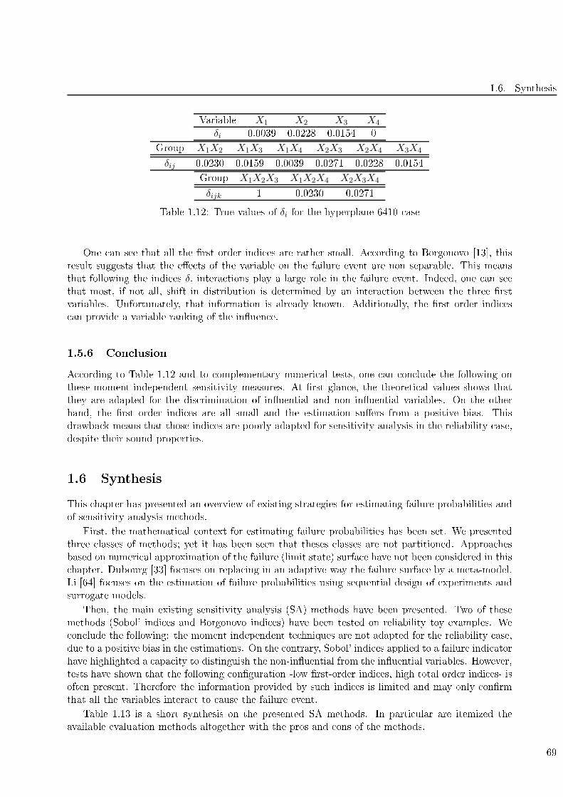
1.6. Synthesis
Variable X1 X2 X3 X4
δi 0.0039 0.0228 0.0154 0
Group X1X2 X1X3 X1X4 X2X3 X2X4 X3X4
δij 0.0230 0.0159 0.0039 0.0271 0.0228 0.0154
Group X1X2X3 X1X2X4 X2X3X4
δijk 1 0.0230 0.0271
Table 1.12: True values of δi for the hyperplane 6410 ase
One an see that all the rst order indi es are rather small. A ording to Borgonovo [13, this
result suggests that the ee ts of the variable on the failure event are non separable. This means
that following the indi es δ, intera tions play a large role in the failure event. Indeed, one an see
that most, if not all, shift in distribution is determined by an intera tion between the three rst
variables. Unfortunately, that information is already known. Additionally, the rst order indi es
an provide a variable ranking of the inuen e.
1.5.6 Con lusion
A ording to Table 1.12 and to omplementary numeri al tests, one an on lude the following on
these moment-independent sensitivity measures. At rst glan e, the theoreti al values shows that
they are adapted for the dis rimination of inuential and non inuential variables. On the other
hand, the rst order indi es are all small and the estimation suers from a positive bias. This
drawba k means that those indi es are poorly adapted for sensitivity analysis in the reliability ase,
despite their sound properties.
1.6 Synthesis
This hapter has presented an overview of existing strategies for estimating failure probabilities and
of sensitivity analysis methods.
First, the mathemati al ontext for estimating failure probabilities has been set. We presented
three lasses of methods; yet it has been seen that theses lasses are not partitioned. Approa hes
based on numeri al approximation of the failure (limit state) surfa e have not been onsidered in this
hapter. Dubourg [33 fo uses on repla ing in an adaptive way the failure surfa e by a meta-model.
Li [64 fo uses on the estimation of failure probabilities using sequential design of experiments and
surrogate models.
Then, the main existing sensitivity analysis (SA) methods have been presented. Two of these
methods (Sobol' indi es and Borgonovo indi es) have been tested on reliability toy examples. We
on lude the following: the moment independent te hniques are not adapted for the reliability ase,
due to a positive bias in the estimations. On the ontrary, Sobol' indi es applied to a failure indi ator
have highlighted a apa ity to distinguish the non-inuential from the inuential variables. However,
tests have shown that the following onguration -low rst-order indi es, high total order indi es- is
often present. Therefore the information provided by su h indi es is limited and may only onrm
that all the variables intera t to ause the failure event.
Table 1.13 is a short synthesis on the presented SA methods. In parti ular are itemized the
available evaluation methods altogether with the pros and ons of the methods.
69
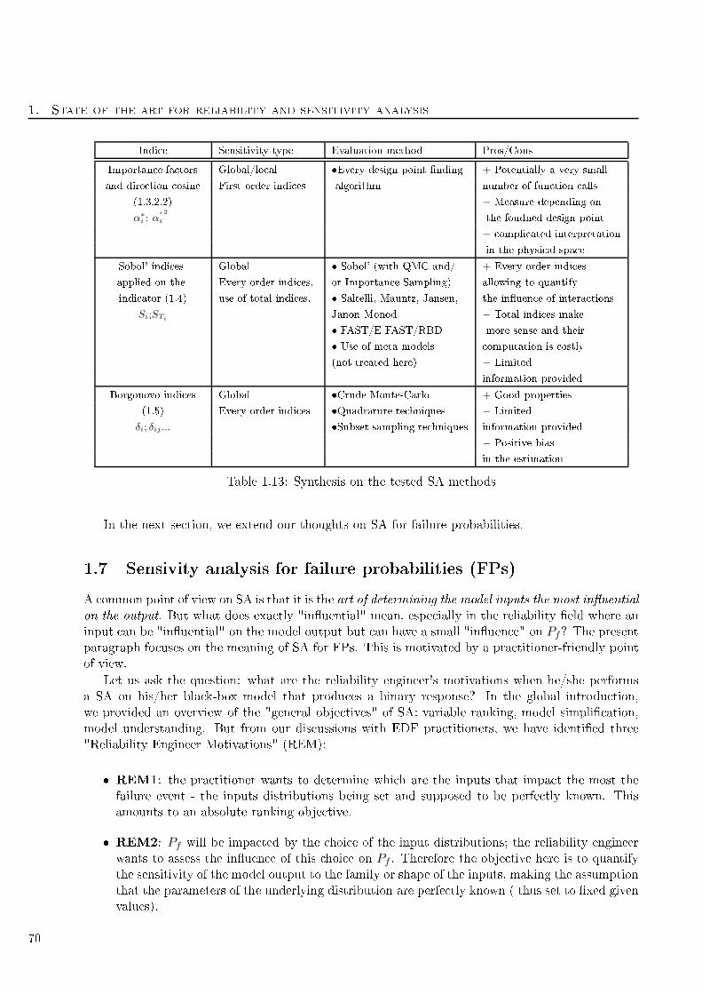
1. State of the art for reliability and sensitivity analysis
Indi e Sensitivity type Evaluation method Pros/Cons
Importan e fa tors Global/lo al Every design point nding + Potentially a very small
and dire tion osine First order indi es algorithm number of fun tion alls
(1.3.2.2) − Measure depending on
α∗i ; α
*
2
i the foudned design point
− ompli ated interpretation
in the physi al spa e
Sobol' indi es Global Sobol' (with QMC and/ + Every order indi es
applied on the Every order indi es, or Importan e Sampling) allowing to quantify
indi ator (1.4) use of total indi es. Saltelli, Mauntz, Jansen, the inuen e of intera tions
Si;STiJanon-Monod − Total indi es make
FAST/E-FAST/RBD more sense and their
Use of meta-models omputation is ostly
(not treated here) − Limited
information provided
Borgonovo indi es Global Crude Monte-Carlo + Good properties
(1.5) Every order indi es Quadrature te hniques − Limited
δi; δij ... Subset sampling te hniques information provided
− Positive bias
in the estimation
Table 1.13: Synthesis on the tested SA methods
In the next se tion, we extend our thoughts on SA for failure probabilities.
1.7 Sensivity analysis for failure probabilities (FPs)
A ommon point of view on SA is that it is the art of determining the model inputs the most inuential
on the output. But what does exa tly "inuential" mean, espe ially in the reliability eld where an
input an be "inuential" on the model output but an have a small "inuen e" on Pf? The present
paragraph fo uses on the meaning of SA for FPs. This is motivated by a pra titioner-friendly point
of view.
Let us ask the question: what are the reliability engineer's motivations when he/she performs
a SA on his/her bla k-box model that produ es a binary response? In the global introdu tion,
we provided an overview of the "general obje tives" of SA: variable ranking, model simpli ation,
model understanding. But from our dis ussions with EDF pra titioners, we have identied three
"Reliability Engineer Motivations" (REM):
REM1: the pra titioner wants to determine whi h are the inputs that impa t the most the
failure event - the inputs distributions being set and supposed to be perfe tly known. This
amounts to an absolute ranking obje tive.
REM2: Pf will be impa ted by the hoi e of the input distributions; the reliability engineer
wants to assess the inuen e of this hoi e on Pf . Therefore the obje tive here is to quantify
the sensitivity of the model output to the family or shape of the inputs, making the assumption
that the parameters of the underlying distribution are perfe tly known ( thus set to xed given
values).
70
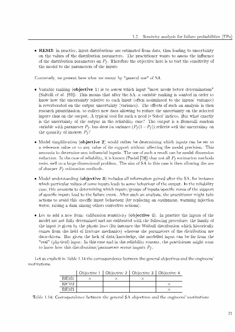
1.7. Sensivity analysis for failure probabilities (FPs)
REM3: in pra ti e, input distributions are estimated from data, thus leading to un ertainty
on the values of the distribution parameters. The pra titioner wants to assess the inuen e
of the distribution parameters on Pf . Therefore the obje tive here is to test the sensitivity of
the model to the parameters of the inputs
Conversely, we present here what we meant by "general use" of SA.
Variable ranking (obje tive 1) is to assess whi h input "most needs better determination"
(Saltelli et al. [89). This means that after the SA, a variable ranking is wanted in order to
know how the un ertainty relative to ea h input (often assimilated to the inputs' varian e)
is reverberated on the output un ertainty (varian e). The ee ts of su h an analysis is then
resear h prioritization, to olle t new data allowing to redu e the un ertainty on the sele ted
inputs thus on the output. A typi al tool for su h a need is Sobol' indi es. But what exa tly
is the un ertainty of the output in the reliability ase? The output is a Bernoulli random
variable with parameter Pf , but does its varian e (Pf (1−Pf )) ree ts well the un ertainty on
the quantity of interest Pf?
Model simpli ation (obje tive 2) would rather be determining whi h inputs an be set to
a referen e value or to any value of its support without ae ting the model pre ision. This
amounts to determine non-inuential inputs. The use of su h a result an be model dimension
redu tion. In the ase of reliability, it is known (Pastel [79) that not all Pf estimation methods
resist well to a large dimensional problem. The aim of SA in this ase is then allowing the use
of sharper Pf estimation methods.
Model understanding (obje tive 3) in ludes all information gained after the SA, for instan e
whi h parti ular values of some inputs leads to some behaviour of the output. In the reliability
ase, this amounts to determining whi h inputs/groups of inputs/spe i zones of the support
of spe i inputs lead to the failure event. After su h an analysis, the pra titioner might take
a tions to avoid this spe i input behaviour (by repla ing an equipment, warming inje tion
water, raising a dam among others orre tive a tions).
Let us add a new item: alibration sensitivity (obje tive 4). In pra ti e the inputs of the
model are not fully determined and are alibrated with the following pro edure: the family of
the input is given by the physi laws (for instan e the Weibull distribution whi h histori ally
omes from the eld of fra ture me hani s) whereas the parameters of the distribution are
data-driven. But given the la k of data/knowledge, the modelled input an be far from the
"real" (physi al) input. In this ase and in the reliability ontext, the pra titioner might want
to know how this distributions/parameters errors impa t Pf .
Let us expli it in Table 1.14 the orresponden e between the general obje tives and the engineers'
motivations.
Obje tive 1 Obje tive 2 Obje tive 3 Obje tive 4
REM1 × × ×REM2 ×REM3 ×
Table 1.14: Corresponden e between the general SA obje tives and the engineers' motivations
71
1. State of the art for reliability and sensitivity analysis
As noti ed in Se tion 1.4, the dire t appli ation of Sobol' indi es on the failure indi ator provides
the following pattern: very small rst order indi es, very large and similarly equal total indi es. The
interpretation of this pattern is that all/most of the variables play an a tive role in the failure event
(obje tive 3) and we an use the total indi es to provide a variable ranking (obje tive 1). However
the answer to both these questions is in pra ti e already known (the pra titioner knows that the
equipment fails when all variables take extreme values at the same time). A ordingly, this method
an in some ases dete ts non-inuential inputs (obje tive 2). But from the pra titioner point of
view, Sobol' indi es only fullls REM1.
In the following of this thesis, we propose 3 spe i methods allowing to answer the dierent
obje tives.
The two rst methods are itemized in Chapter 2 and provide a variable ranking (obje tive 1,
REM1). Spe i ally, the rst method makes use of sensitivity indi es produ ed by a lassi ation
method (random forests). The se ond method measures the departure, at ea h step of a subset
method, between ea h input original density and the density given the subset rea hed.
The method presented in Chapter 3 will be referred to as Density Modi ation Based Reliability
Sensitivity Indi es (DMBSRI). These indi es altogether with their estimation methods have been
initially presented in Lemaître and Arnaud [62 then in Lemaître et al. [63. They are based upon
an input pdf modi ation, and quantify the impa t of su h a modi ation on the FP. We argue that
with an adapted perturbation, this method an fulll the four presented general uses (obje tive 1 to
4), altogether with the three engineers' motivations (REM1 to 3). This will be developed further in
se tion 3.3.3.
72
Chapter 2
Variable ranking in the reliability ontext
2.1 Introdu tion
As stated in Se tion 1.7, there is a need in SA for te hniques produ ing a variable ranking (REM1,
obje tive 1). This hapter presents two methods allowing to rank the random inputs by their
inuen e on the output. Furthermore, these methods are thoughts as by-produ ts of the estimation
of the failure probability Pf . Indeed the rst te hnique (Se tion 2.2) proposes to make use of
lassi ation trees and random forests built on a MC sample. The se ond te hnique (Se tion 2.3)
measures the departure, at ea h step of a subset method, between ea h input original density and
the density given the subset rea hed. Thus both of these methods are by-produ ts of two sampling
te hniques. Se tion 2.4 summarises the hapter and proposes a on lusion.
2.2 Using lassi ation trees and random forests in SA
Classi ation trees and random forests are two well-known lassi ation te hniques. Additionally,
sensitivity measures an be derived. This se tion aims at introdu ing these te hniques. A state of
the art on lassi ation trees is proposed in 2.2.1. A subse tion introdu ing the main stabilisation
methods (su h as random forests) is then studied in 2.2.2. Variable ranking te hniques are derived in
2.2.3. The variable ranking is then tested on the usual ases in 2.2.4. A dis ussion is then proposed
in 2.2.5, where the main theme is the improvement of models.
2.2.1 State of the art for lassi ation trees
This se tion is widely inspired by Besse [11; parts 3 and 4 of Briand [19; but also parts 1 and
2 of Genuer [39 (in Fren h). All those ontributions are inspired by the founding monograph by
Breiman et al. [17. An introdu tion on statisti al learning and the growing of lassi ation tree
an also be found in Hastie et al. [44.
Sample Let us assume that we have an input sample of j = 1, . . . , N observations from d explana-tory variables (or inputs) onsidered as quantitative, denoted by Xj
i , i = 1, . . . , d. A quantitative
variable Y jwith two modalities is asso iated with these realisations of the inputs. Let us assume
that the values taken by Y are in 0, 1. In the onsidered framework, this sample might be the
result of a Monte-Carlo experiment for a omputer model where the quantity of interest is a prob-
ability of ex eeding a given threshold (the events are failure/non-failure of the system). A sample
aggregating the inputs and output of a subset simulation might also be used - this ase is dis ussed
73
2. Variable ranking in the reliability ontext
in Se tion 2.2.5. The sample is divided in two parts: a training set and a test set. The training set
is used to t the model (in the next se tion, the lassi ation tree). The test set is used to assess
the generalization error of the model (Hastie et al. [44).
Growing a binary tree A lassi ation tree is built by re ursive partitioning of the input spa e.
Fo us will be set on the CART (Classi ation And Regression Tree) method, Breiman et al. [17.
Moreover, the regression ase will not be treated here.
The growth (or tting) of a lassi ation tree is done in sele ting a sequen e of nodes (binary
partition of the input spa e) then in determining a subsequen e (pruning) that will be optimal
a ording to a given riterion A node is dened by an input variable (splitting variable) and a
division, allowing the separation of the sample in two subsamples. A division is dened by a value
(split point). At the rst node (also referred to as root of the tree) orresponds the whole sample;
then iterations are made on the produ ed subsamples.
The algorithm requires :
the denition of a riterion allowing to sele t the best node (variable+division);
a rule to end the algorithm and de ide that a node is terminal (also referred to as leaf);
a rule to assign a terminal node to a lass.
Division riterion Ea h variable (1, . . . , d) produ es N − 1 allowed splits (that is to say reating
a non-empty node). There are d × (m − 1) allowed splits in whi h the optimal division must be
hosen. The division riterion is related to a node impurity measure: the aim is to obtain nodes as
homogeneous as possible with respe t to the output Y . The impurity measure onsiders the mixture
of Y 's modality in a node. It is null if and only if all the individuals of the same node share the
same value of Y . It is maximal when the modalities of Y are equally present in the node.
The devian e (or heterogeneity) of a node k is denoted Dk. The redu tion of devian e (or
impurity redu tion) from splitting this node into des ending nodes t and s would then be:
∆D = Dk −Dt −Ds
.
The tree is built by taking the maximum redu tion in devian e over the allowed splits:
maxallowed splits δ
Dk − (Dt +Ds)
Stopping rule The algorithm stops for a given node when it is homogeneous (it ontains a single
lass and therefore annot be divided no more). The algorithm an also be alibrated to avoid
useless splits: the division pro ess is stopped when the number of values in the node is less than a
xed size (for instan e 5 individuals).
Ae tation rule If the terminal node (leaf) is homogeneous, it is ae ted to the represented
lass. If not, a majority rule is applied. If wrong- lassi ation osts are given, the less ostly lass
is hosen.
74
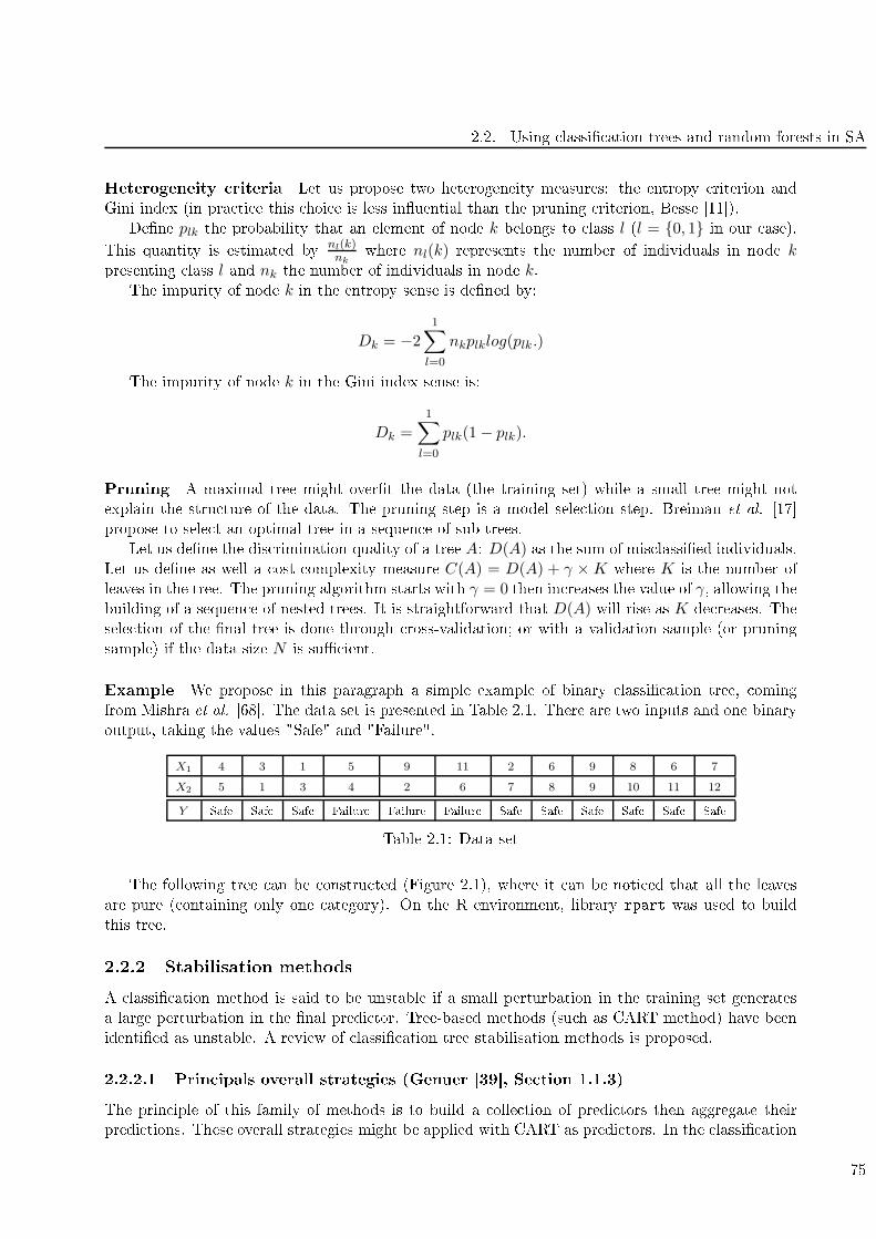
2.2. Using lassi ation trees and random forests in SA
Heterogeneity riteria Let us propose two heterogeneity measures: the entropy riterion and
Gini index (in pra ti e this hoi e is less inuential than the pruning riterion, Besse [11).
Dene plk the probability that an element of node k belongs to lass l (l = 0, 1 in our ase).
This quantity is estimated by
nl(k)nk
where nl(k) represents the number of individuals in node kpresenting lass l and nk the number of individuals in node k.
The impurity of node k in the entropy sense is dened by:
Dk = −2
1∑
l=0
nkplklog(plk.)
The impurity of node k in the Gini index sense is:
Dk =
1∑
l=0
plk(1− plk).
Pruning A maximal tree might overt the data (the training set) while a small tree might not
explain the stru ture of the data. The pruning step is a model sele tion step. Breiman et al. [17
propose to sele t an optimal tree in a sequen e of sub-trees.
Let us dene the dis rimination quality of a tree A: D(A) as the sum of mis lassied individuals.
Let us dene as well a ost- omplexity measure C(A) = D(A) + γ ×K where K is the number of
leaves in the tree. The pruning algorithm starts with γ = 0 then in reases the value of γ, allowing thebuilding of a sequen e of nested trees. It is straightforward that D(A) will rise as K de reases. The
sele tion of the nal tree is done through ross-validation; or with a validation sample (or pruning
sample) if the data size N is su ient.
Example We propose in this paragraph a simple example of binary lassi ation tree, oming
from Mishra et al. [68. The data set is presented in Table 2.1. There are two inputs and one binary
output, taking the values "Safe" and "Failure".
X1 4 3 1 5 9 11 2 6 9 8 6 7
X2 5 1 3 4 2 6 7 8 9 10 11 12
Y Safe Safe Safe Failure Failure Failure Safe Safe Safe Safe Safe Safe
Table 2.1: Data set
The following tree an be onstru ted (Figure 2.1), where it an be noti ed that all the leaves
are pure ( ontaining only one ategory). On the R environment, library rpart was used to build
this tree.
2.2.2 Stabilisation methods
A lassi ation method is said to be unstable if a small perturbation in the training set generates
a large perturbation in the nal predi tor. Tree-based methods (su h as CART method) have been
identied as unstable. A review of lassi ation tree stabilisation methods is proposed.
2.2.2.1 Prin ipals overall strategies (Genuer [39, Se tion 1.1.3)
The prin iple of this family of methods is to build a olle tion of predi tors then aggregate their
predi tions. These overall strategies might be applied with CART as predi tors. In the lassi ation
75

2. Variable ranking in the reliability ontext
x2 < 6.5
x1 >= 4.5
Failure Safe
Safe
yes no
Figure 2.1: Binary tree
ase, the aggregation is done with a majority vote. The aim of this lass of methods is to avoid
overt.
Bagging Proposed by Breiman [15 with CART as predi tors, bagging is the ontra tion of
bootstrap aggregating. The main idea is to build, from the training sample, a number of bootstrap
samples, then to aggregate the predi tions. The generi bagging algorithm is presented in Algorithm
1. In our parti ular ase, the hosen predi tor is the lassi ation tree of CART.
Algorithm 1 Bagging
Let X0be a set of inputs for whi h a fore ast is wanted and Z = (Xj , Y j)j=1,...,N a training sample.
For b = 1, . . . , B do:
Sample a bootstrap sample Zb
Estimate the predi tor hZbon this sample
End for
Compute the mean predi tion hB(X0) = argmaxj #
b|hZb
(X0) = j.
Boosting Proposed by Freund et Shapire [36, this type of algorithm is widely used with CART
as predi tors.
The prin iple is the sequential onstru tion of models in whi h important weights are ae ted to
mis lassied individuals. The founding algorithm Adaboost (Adaptive boosting) is des ribed in the
ase of a dis rimination problem with two lasses −1, 1. An initial bootstrap sample is sampled,
where ea h individual has the same probability to appear. A lassier (predi tor) is estimated,
altogether with its lassi ation error. A se ond bootstrap sample is generated, where mis lassied
individuals are more likely to appear. Another predi tor is tted and the algorithm ontinues.
Ea h sample is generated a ording to the performan e of the previous lassier. At the end, all
76
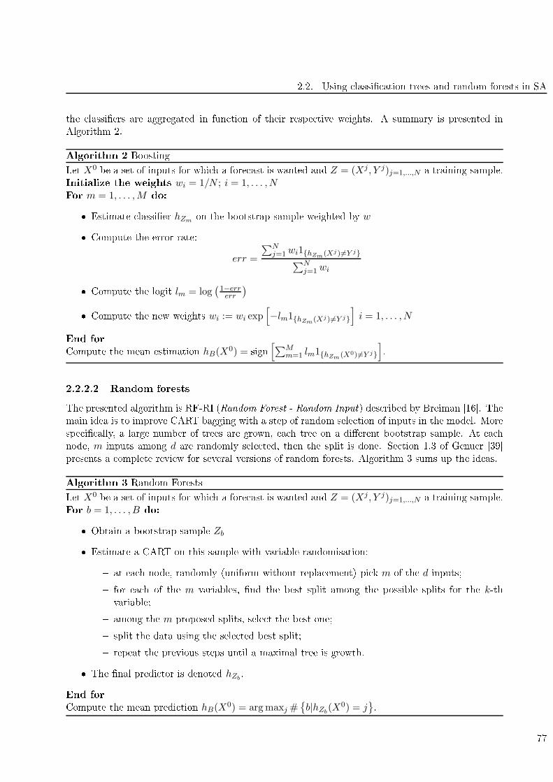
2.2. Using lassi ation trees and random forests in SA
the lassiers are aggregated in fun tion of their respe tive weights. A summary is presented in
Algorithm 2.
Algorithm 2 Boosting
Let X0be a set of inputs for whi h a fore ast is wanted and Z = (Xj , Y j)j=1,...,N a training sample.
Initialize the weights wi = 1/N ; i = 1, . . . , NFor m = 1, . . . ,M do:
Estimate lassier hZm on the bootstrap sample weighted by w
Compute the error rate:
err =
∑Nj=1wi1hZm(Xj )6=Y j∑N
j=1wi
Compute the logit lm = log(1−errerr
)
Compute the new weights wi := wi exp[−lm1hZm(Xj )6=Y j
]i = 1, . . . , N
End for
Compute the mean estimation hB(X0) = sign
[∑Mm=1 lm1hZm(X0)6=Y j
].
2.2.2.2 Random forests
The presented algorithm is RF-RI (Random Forest - Random Input) des ribed by Breiman [16. The
main idea is to improve CART bagging with a step of random sele tion of inputs in the model. More
spe i ally, a large number of trees are grown, ea h tree on a dierent bootstrap sample. At ea h
node, m inputs among d are randomly sele ted, then the split is done. Se tion 1.3 of Genuer [39
presents a omplete review for several versions of random forests. Algorithm 3 sums up the ideas.
Algorithm 3 Random Forests
Let X0be a set of inputs for whi h a fore ast is wanted and Z = (Xj , Y j)j=1,...,N a training sample.
For b = 1, . . . , B do:
Obtain a bootstrap sample Zb
Estimate a CART on this sample with variable randomisation:
at ea h node, randomly (uniform without repla ement) pi k m of the d inputs;
for ea h of the m variables, nd the best split among the possible splits for the k-thvariable;
among the m proposed splits, sele t the best one;
split the data using the sele ted best split;
repeat the previous steps until a maximal tree is growth.
The nal predi tor is denoted hZb.
End for
Compute the mean predi tion hB(X0) = argmaxj #
b|hZb
(X0) = j.
77
2. Variable ranking in the reliability ontext
The default value for m in the lassi ation ontext is m =√d. Noti e that ea h tree is maximal
and is not pruned. Some theoreti al results on pure random forests (PRF) are available in Biau [12.
2.2.2.3 Stru ture stabilisation methods (Briand [19, se tion 4.4)
The presented stabilisation methods su h as Bagging and Random Forests onsist in the onstru tion
of a large number of lassiers on a randomized sample. These te hniques improve the apa ity of
the predi tors but the singular tree stru ture is lost. This singularity might be a requirement when
the aim of the lassi ation is the proposal of a de ision tree. The te hniques proposed hereafter
aims at keeping the stru ture of the tree by stabilizing the nodes.
The method proposed by Ruey-Hsia [86 onsists in in luding, for ea h node, logi al stru tures.
For instan e, a division riterion might be "2 ≤ Xi and Xk ≥ 5". The notion used to rea h su h a
result is the existen e of a division "almost as good" as the optimal. Briand [19 remarks that the
existen e of a large number of logi al expressions might ompli ate the interpretation of the tree.
Choi e is then set to use a method allowing a stabilisation of the nodes (division and variable
asso iated) of the tree. The inspiration omes from Dannegger [29. The main idea is to re-sample in
a bootstrap fashion for ea h node. For ea h sample, the optimal division is sear hed. The variables
most frequently sele ted are then used as a division variable for the treated node.
Briand proposed Dannegger's algorithm to build a maximal tree, then to prune the tree with
a redu ed error pruning method, Quinlan [81. The ouple tree growing/pruning is denoted REN
method. An arti le by Briand et al. [20 proposes a similarity measure between trees - that might
be of dierent stru tures. This similarity measure is used in Briand [19 to ompare trees built with
CART method or with REN method. It allows to assess the stability of the REN method to build
lassi ation trees.
2.2.3 Variable importan e - Sensitivity analysis
2.2.3.1 Criteria denition
Tree-based lassi ation methods are mostly used in the genomi domain, where the number of
variables is mu h higher than the number of observations (N ≪ d). Thereby, dierent importan e
measures have been onsidered by several authors. These measures are presented here, reminding
that their aim is the sele tion of a few inputs among a large number of explanatory variables.
CART ase A naive idea of variable ranking is that the variables most involved in the partition
(and espe ially those whi h nodes are lose from the root) are the most inuential. A more rened
idea has been proposed by Breiman et al. [17. It is dened as the sum on the nodes of the
heterogeneity redu tion (for substitution divisions). An introdu tion on this index is presented in
Ghattas [40. It is also used altogether with the REN stabilisation method of Briand.
RFRI ase When building a large number of trees, and randomizing ea h onstru tion step, the
unique stru ture des ribed in the CART ase is lost. Thereby, new sensitivity measures are proposed
by Breiman [16.
A rst naive estimator of a variable's inuen e is the frequen y of its apparition in the forest.
A se ond estimator is said to be "lo al", it is based on the sum of the heterogeneity redu tion
(in the Gini index sense) on nodes where the variable is used. This riterion will be denoted
GI in the following. The importan e riterion VGI is the sum of the heterogeneity de rease
due to variable Xi, divided by the number of trees in the forest Ntrees.
78
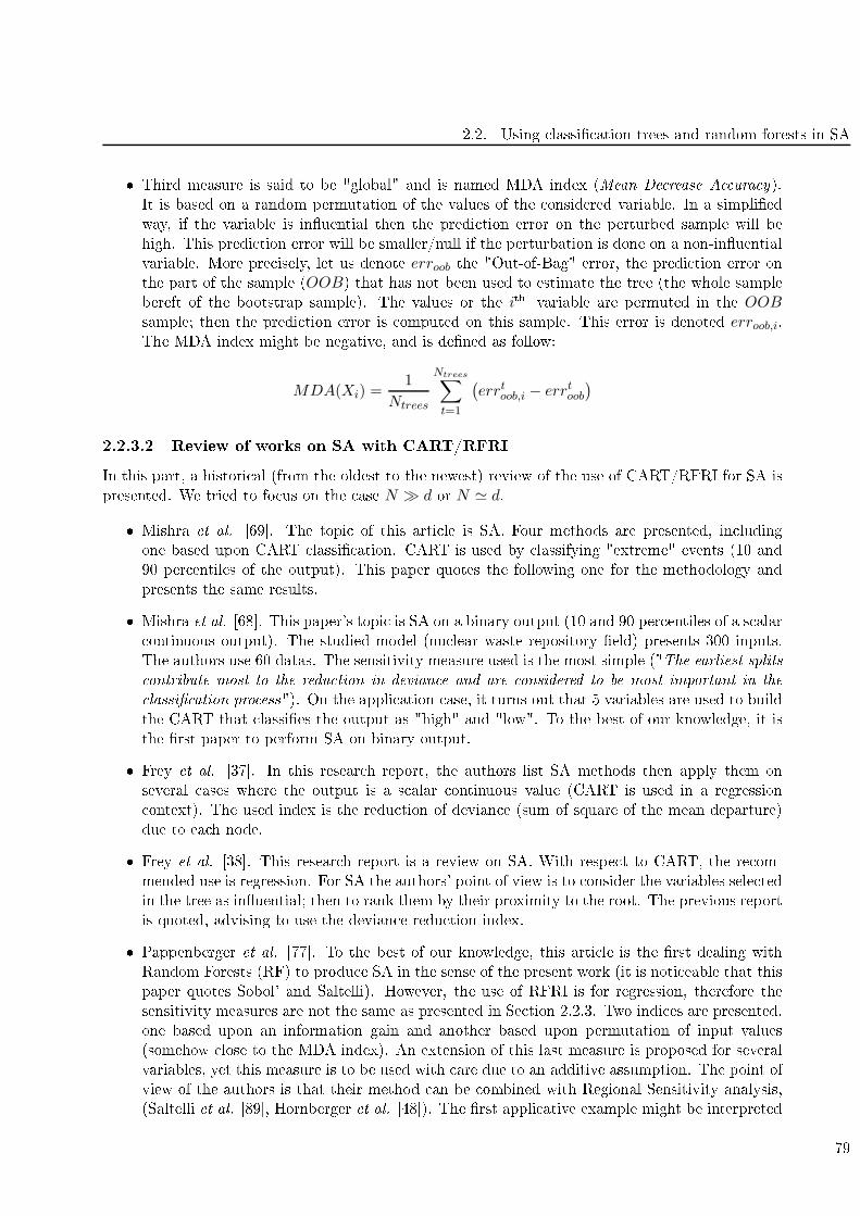
2.2. Using lassi ation trees and random forests in SA
Third measure is said to be "global" and is named MDA index (Mean De rease A ura y).
It is based on a random permutation of the values of the onsidered variable. In a simplied
way, if the variable is inuential then the predi tion error on the perturbed sample will be
high. This predi tion error will be smaller/null if the perturbation is done on a non-inuential
variable. More pre isely, let us denote erroob the "Out-of-Bag" error, the predi tion error on
the part of the sample (OOB) that has not been used to estimate the tree (the whole sample
bereft of the bootstrap sample). The values or the ith variable are permuted in the OOBsample; then the predi tion error is omputed on this sample. This error is denoted erroob,i.The MDA index might be negative, and is dened as follow:
MDA(Xi) =1
Ntrees
Ntrees∑
t=1
(errtoob,i − errtoob
)
2.2.3.2 Review of works on SA with CART/RFRI
In this part, a histori al (from the oldest to the newest) review of the use of CART/RFRI for SA is
presented. We tried to fo us on the ase N ≫ d or N ≃ d.
Mishra et al. [69. The topi of this arti le is SA. Four methods are presented, in luding
one based upon CART lassi ation. CART is used by lassifying "extreme" events (10 and
90 per entiles of the output). This paper quotes the following one for the methodology and
presents the same results.
Mishra et al. [68. This paper's topi is SA on a binary output (10 and 90 per entiles of a s alar
ontinuous output). The studied model (nu lear waste repository eld) presents 300 inputs.
The authors use 60 datas. The sensitivity measure used is the most simple ("The earliest splits
ontribute most to the redu tion in devian e and are onsidered to be most important in the
lassi ation pro ess"). On the appli ation ase, it turns out that 5 variables are used to build
the CART that lassies the output as "high" and "low". To the best of our knowledge, it is
the rst paper to perform SA on binary output.
Frey et al. [37. In this resear h report, the authors list SA methods then apply them on
several ases where the output is a s alar ontinuous value (CART is used in a regression
ontext). The used index is the redu tion of devian e (sum of square of the mean departure)
due to ea h node.
Frey et al. [38. This resear h report is a review on SA. With respe t to CART, the re om-
mended use is regression. For SA the authors' point of view is to onsider the variables sele ted
in the tree as inuential; then to rank them by their proximity to the root. The previous report
is quoted, advising to use the devian e redu tion index.
Pappenberger et al. [77. To the best of our knowledge, this arti le is the rst dealing with
Random Forests (RF) to produ e SA in the sense of the present work (it is noti eable that this
paper quotes Sobol' and Saltelli). However, the use of RFRI is for regression, therefore the
sensitivity measures are not the same as presented in Se tion 2.2.3. Two indi es are presented,
one based upon an information gain and another based upon permutation of input values
(somehow lose to the MDA index). An extension of this last measure is proposed for several
variables, yet this measure is to be used with are due to an additive assumption. The point of
view of the authors is that their method an be ombined with Regional Sensitivity analysis,
(Saltelli et al. [89, Hornberger et al. [48). The rst appli ative example might be interpreted
79
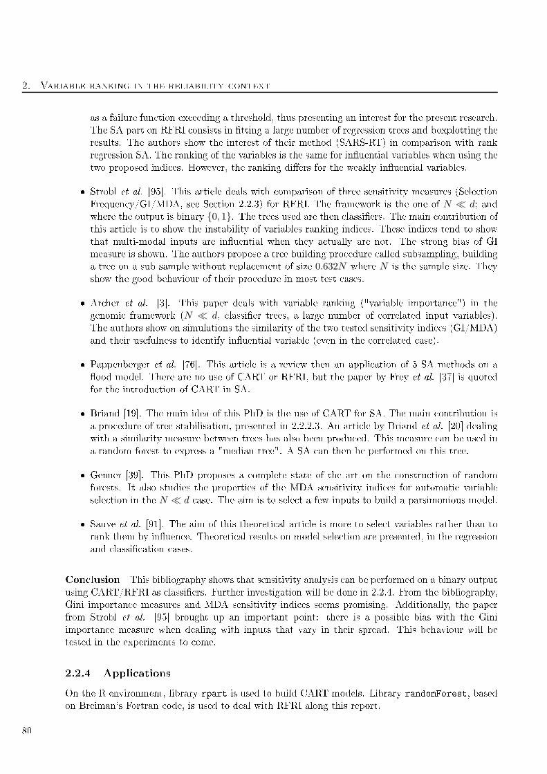
2. Variable ranking in the reliability ontext
as a failure fun tion ex eeding a threshold, thus presenting an interest for the present resear h.
The SA part on RFRI onsists in tting a large number of regression trees and boxplotting the
results. The authors show the interest of their method (SARS-RT) in omparison with rank
regression SA. The ranking of the variables is the same for inuential variables when using the
two proposed indi es. However, the ranking diers for the weakly inuential variables.
Strobl et al. [95. This arti le deals with omparison of three sensitivity measures (Sele tion
Frequen y/GI/MDA, see Se tion 2.2.3) for RFRI. The framework is the one of N ≪ d; andwhere the output is binary 0, 1. The trees used are then lassiers. The main ontribution of
this arti le is to show the instability of variables ranking indi es. These indi es tend to show
that multi-modal inputs are inuential when they a tually are not. The strong bias of GI
measure is shown. The authors propose a tree building pro edure alled subsampling, building
a tree on a sub sample without repla ement of size 0.632N where N is the sample size. They
show the good behaviour of their pro edure in most test ases.
Ar her et al. [3. This paper deals with variable ranking ("variable importan e") in the
genomi framework (N ≪ d, lassier trees, a large number of orrelated input variables).
The authors show on simulations the similarity of the two tested sensitivity indi es (GI/MDA)
and their usefulness to identify inuential variable (even in the orrelated ase).
Pappenberger et al. [76. This arti le is a review then an appli ation of 5 SA methods on a
ood model. There are no use of CART or RFRI, but the paper by Frey et al. [37 is quoted
for the introdu tion of CART in SA.
Briand [19. The main idea of this PhD is the use of CART for SA. The main ontribution is
a pro edure of tree stabilisation, presented in 2.2.2.3. An arti le by Briand et al. [20 dealing
with a similarity measure between trees has also been produ ed. This measure an be used in
a random forest to express a "median tree". A SA an then be performed on this tree.
Genuer [39. This PhD proposes a omplete state of the art on the onstru tion of random
forests. It also studies the properties of the MDA sensitivity indi es for automati variable
sele tion in the N ≪ d ase. The aim is to sele t a few inputs to build a parsimonious model.
Sauve et al. [91. The aim of this theoreti al arti le is more to sele t variables rather than to
rank them by inuen e. Theoreti al results on model sele tion are presented, in the regression
and lassi ation ases.
Con lusion This bibliography shows that sensitivity analysis an be performed on a binary output
using CART/RFRI as lassiers. Further investigation will be done in 2.2.4. From the bibliography,
Gini importan e measures and MDA sensitivity indi es seems promising. Additionally, the paper
from Strobl et al. [95 brought up an important point: there is a possible bias with the Gini
importan e measure when dealing with inputs that vary in their spread. This behaviour will be
tested in the experiments to ome.
2.2.4 Appli ations
On the R environment, library rpart is used to build CART models. Library randomForest, based
on Breiman's Fortran ode, is used to deal with RFRI along this report.
80
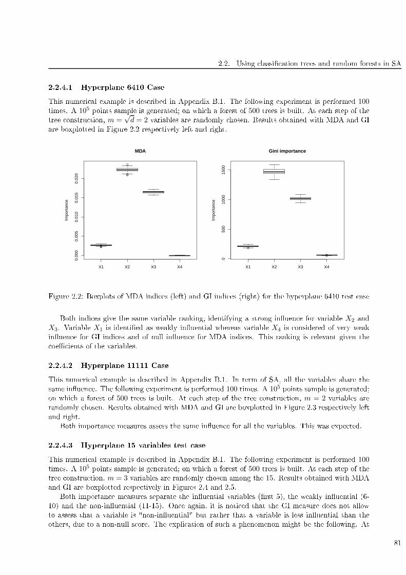
2.2. Using lassi ation trees and random forests in SA
2.2.4.1 Hyperplane 6410 Case
This numeri al example is des ribed in Appendix B.1. The following experiment is performed 100times. A 105 points sample is generated; on whi h a forest of 500 trees is built. At ea h step of the
tree onstru tion, m =√d = 2 variables are randomly hosen. Results obtained with MDA and GI
are boxplotted in Figure 2.2 respe tively left and right.
0.00
00.
005
0.01
00.
015
0.02
0
MDA
Impo
rtan
ce
X1 X2 X3 X4
050
010
0015
00
Gini importance
Impo
rtan
ce
X1 X2 X3 X4
Figure 2.2: Boxplots of MDA indi es (left) and GI indi es (right) for the hyperplane 6410 test ase
Both indi es give the same variable ranking, identifying a strong inuen e for variable X2 and
X3. Variable X1 is identied as weakly inuential whereas variable X4 is onsidered of very weak
inuen e for GI indi es and of null inuen e for MDA indi es. This ranking is relevant given the
oe ients of the variables.
2.2.4.2 Hyperplane 11111 Case
This numeri al example is des ribed in Appendix B.1. In term of SA, all the variables share the
same inuen e. The following experiment is performed 100 times. A 105 points sample is generated;
on whi h a forest of 500 trees is built. At ea h step of the tree onstru tion, m = 2 variables are
randomly hosen. Results obtained with MDA and GI are boxplotted in Figure 2.3 respe tively left
and right.
Both importan e measures assess the same inuen e for all the variables. This was expe ted.
2.2.4.3 Hyperplane 15 variables test ase
This numeri al example is des ribed in Appendix B.1. The following experiment is performed 100times. A 105 points sample is generated; on whi h a forest of 500 trees is built. At ea h step of the
tree onstru tion, m = 3 variables are randomly hosen among the 15. Results obtained with MDA
and GI are boxplotted respe tively in Figures 2.4 and 2.5.
Both importan e measures separate the inuential variables (rst 5), the weakly inuential (6-
10) and the non-inuential (11-15). On e again, it is noti ed that the GI measure does not allow
to assess that a variable is "non-inuential" but rather that a variable is less inuential than the
others, due to a non-null s ore. The expli ation of su h a phenomenon might be the following. At
81
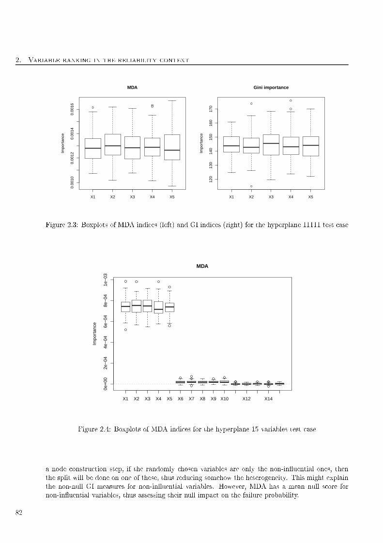
2. Variable ranking in the reliability ontext
0.00
100.
0012
0.00
140.
0016
MDA
Impo
rtan
ce
X1 X2 X3 X4 X5
120
130
140
150
160
170
Gini importance
Impo
rtan
ceX1 X2 X3 X4 X5
Figure 2.3: Boxplots of MDA indi es (left) and GI indi es (right) for the hyperplane 11111 test ase
0e+
002e
−04
4e−
046e
−04
8e−
041e
−03
MDA
Impo
rtan
ce
X1 X2 X3 X4 X5 X6 X7 X8 X9 X10 X12 X14
Figure 2.4: Boxplots of MDA indi es for the hyperplane 15 variables test ase
a node onstru tion step, if the randomly hosen variables are only the non-inuential ones, then
the split will be done on one of these, thus redu ing somehow the heterogeneity. This might explain
the non-null GI measures for non-inuential variables. However, MDA has a mean null s ore for
non-inuential variables, thus assessing their null impa t on the failure probability.
82
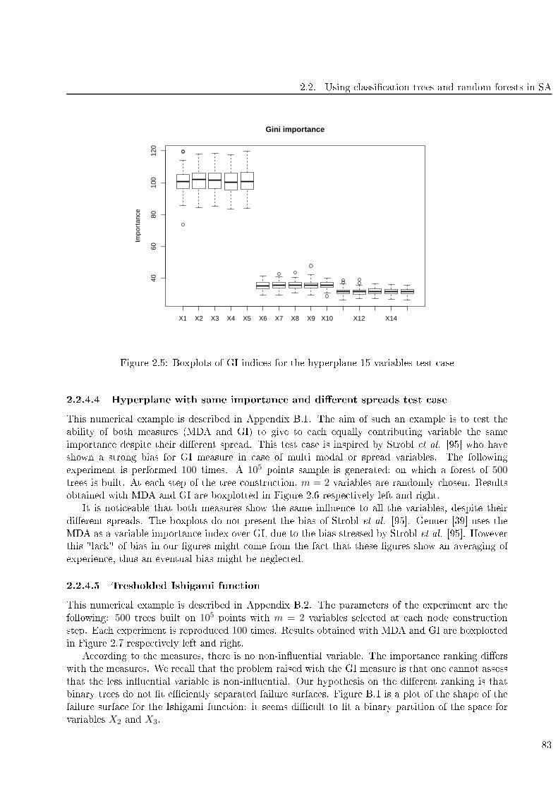
2.2. Using lassi ation trees and random forests in SA
4060
8010
012
0
Gini importanceIm
port
ance
X1 X2 X3 X4 X5 X6 X7 X8 X9 X10 X12 X14
Figure 2.5: Boxplots of GI indi es for the hyperplane 15 variables test ase
2.2.4.4 Hyperplane with same importan e and dierent spreads test ase
This numeri al example is des ribed in Appendix B.1. The aim of su h an example is to test the
ability of both measures (MDA and GI) to give to ea h equally ontributing variable the same
importan e despite their dierent spread. This test ase is inspired by Strobl et al. [95 who have
shown a strong bias for GI measure in ase of multi modal or spread variables. The following
experiment is performed 100 times. A 105 points sample is generated; on whi h a forest of 500trees is built. At ea h step of the tree onstru tion, m = 2 variables are randomly hosen. Results
obtained with MDA and GI are boxplotted in Figure 2.6 respe tively left and right.
It is noti eable that both measures show the same inuen e to all the variables, despite their
dierent spreads. The boxplots do not present the bias of Strobl et al. [95. Genuer [39 uses the
MDA as a variable importan e index over GI, due to the bias stressed by Strobl et al. [95. However
this "la k" of bias in our gures might ome from the fa t that these gures show an averaging of
experien e, thus an eventual bias might be negle ted.
2.2.4.5 Tresholded Ishigami fun tion
This numeri al example is des ribed in Appendix B.2. The parameters of the experiment are the
following: 500 trees built on 105 points with m = 2 variables sele ted at ea h node onstru tion
step. Ea h experiment is reprodu ed 100 times. Results obtained with MDA and GI are boxplotted
in Figure 2.7 respe tively left and right.
A ording to the measures, there is no non-inuential variable. The importan e ranking diers
with the measures. We re all that the problem raised with the GI measure is that one annot assess
that the less inuential variable is non-inuential. Our hypothesis on the dierent ranking is that
binary trees do not t e iently separated failure surfa es. Figure B.1 is a plot of the shape of the
failure surfa e for the Ishigami fun tion: it seems di ult to t a binary partition of the spa e for
variables X2 and X3.
83
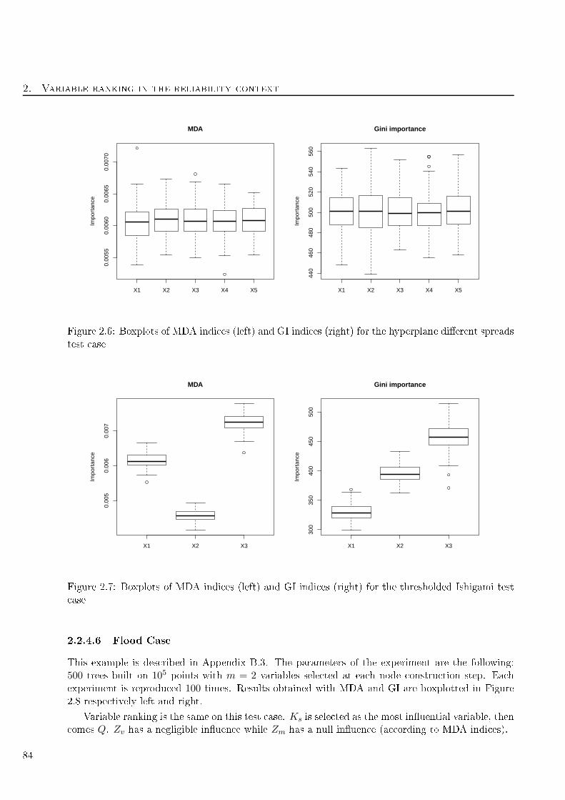
2. Variable ranking in the reliability ontext
0.00
550.
0060
0.00
650.
0070
MDA
Impo
rtan
ce
X1 X2 X3 X4 X5
440
460
480
500
520
540
560
Gini importance
Impo
rtan
ceX1 X2 X3 X4 X5
Figure 2.6: Boxplots of MDA indi es (left) and GI indi es (right) for the hyperplane dierent spreads
test ase
0.00
50.
006
0.00
7
MDA
Impo
rtan
ce
X1 X2 X3
300
350
400
450
500
Gini importance
Impo
rtan
ce
X1 X2 X3
Figure 2.7: Boxplots of MDA indi es (left) and GI indi es (right) for the thresholded Ishigami test
ase
2.2.4.6 Flood Case
This example is des ribed in Appendix B.3. The parameters of the experiment are the following:
500 trees built on 105 points with m = 2 variables sele ted at ea h node onstru tion step. Ea h
experiment is reprodu ed 100 times. Results obtained with MDA and GI are boxplotted in Figure
2.8 respe tively left and right.
Variable ranking is the same on this test ase. Ks is sele ted as the most inuential variable, then
omes Q. Zv has a negligible inuen e while Zm has a null inuen e (a ording to MDA indi es).
84
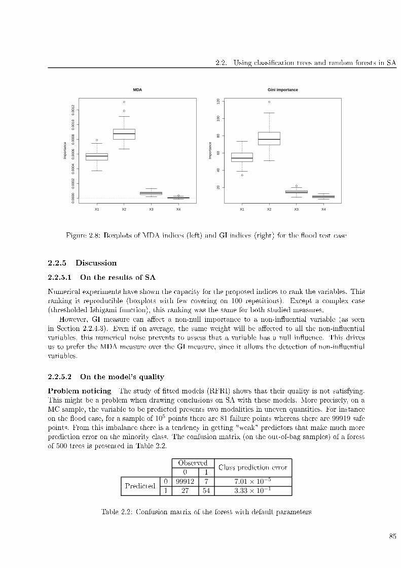
2.2. Using lassi ation trees and random forests in SA
0.00
000.
0002
0.00
040.
0006
0.00
080.
0010
0.00
12
MDA
Impo
rtan
ce
X1 X2 X3 X4
2040
6080
100
120
Gini importance
Impo
rtan
ceX1 X2 X3 X4
Figure 2.8: Boxplots of MDA indi es (left) and GI indi es (right) for the ood test ase
2.2.5 Dis ussion
2.2.5.1 On the results of SA
Numeri al experiments have shown the apa ity for the proposed indi es to rank the variables. This
ranking is reprodu ible (boxplots with few overing on 100 repetitions). Ex ept a omplex ase
(thresholded Ishigami fun tion), this ranking was the same for both studied measures.
However, GI measure an ae t a non-null importan e to a non-inuential variable (as seen
in Se tion 2.2.4.3). Even if on average, the same weight will be ae ted to all the non-inuential
variables, this numeri al noise prevents to assess that a variable has a null inuen e. This drives
us to prefer the MDA measure over the GI measure, sin e it allows the dete tion of non-inuential
variables.
2.2.5.2 On the model's quality
Problem noti ing The study of tted models (RFRI) shows that their quality is not satisfying.
This might be a problem when drawing on lusions on SA with these models. More pre isely, on a
MC sample, the variable to be predi ted presents two modalities in uneven quantities. For instan e
on the ood ase, for a sample of 105 points there are 81 failure points whereas there are 99919 safe
points. From this imbalan e there is a tenden y in getting "weak" predi tors that make mu h more
predi tion error on the minority lass. The onfusion matrix (on the out-of-bag samples) of a forest
of 500 trees is presented in Table 2.2.
Observed
Class predi tion error
0 1
Predi ted
0 99912 7 7.01× 10⁻⁵
1 27 54 3.33× 10⁻¹
Table 2.2: Confusion matrix of the forest with default parameters
85
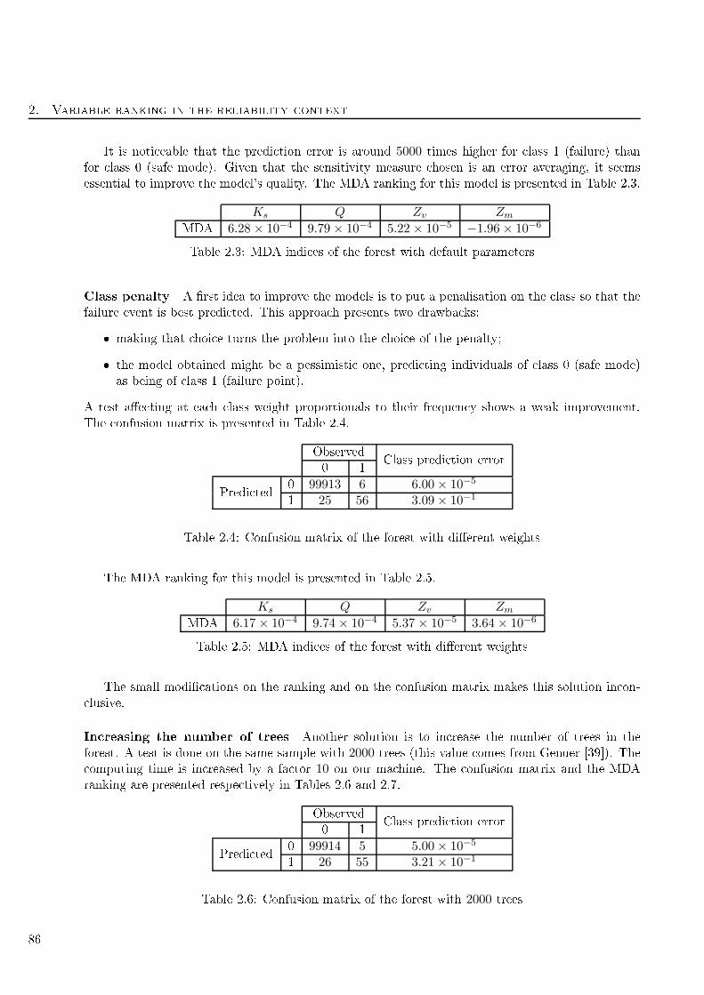
2. Variable ranking in the reliability ontext
It is noti eable that the predi tion error is around 5000 times higher for lass 1 (failure) than
for lass 0 (safe mode). Given that the sensitivity measure hosen is an error averaging, it seems
essential to improve the model's quality. The MDA ranking for this model is presented in Table 2.3.
Ks Q Zv Zm
MDA 6.28 × 10⁻⁴ 9.79 × 10⁻⁴ 5.22 × 10⁻⁵ −1.96 × 10⁻⁶
Table 2.3: MDA indi es of the forest with default parameters
Class penalty A rst idea to improve the models is to put a penalisation on the lass so that the
failure event is best predi ted. This approa h presents two drawba ks:
making that hoi e turns the problem into the hoi e of the penalty;
the model obtained might be a pessimisti one, predi ting individuals of lass 0 (safe mode)
as being of lass 1 (failure point).
A test ae ting at ea h lass weight proportionals to their frequen y shows a weak improvement.
The onfusion matrix is presented in Table 2.4.
Observed
Class predi tion error
0 1
Predi ted
0 99913 6 6.00× 10⁻⁵
1 25 56 3.09× 10⁻¹
Table 2.4: Confusion matrix of the forest with dierent weights
The MDA ranking for this model is presented in Table 2.5.
Ks Q Zv Zm
MDA 6.17× 10⁻⁴ 9.74× 10⁻⁴ 5.37 × 10⁻⁵ 3.64 × 10⁻⁶
Table 2.5: MDA indi es of the forest with dierent weights
The small modi ations on the ranking and on the onfusion matrix makes this solution in on-
lusive.
In reasing the number of trees Another solution is to in rease the number of trees in the
forest. A test is done on the same sample with 2000 trees (this value omes from Genuer [39). The
omputing time is in reased by a fa tor 10 on our ma hine. The onfusion matrix and the MDA
ranking are presented respe tively in Tables 2.6 and 2.7.
Observed
Class predi tion error
0 1
Predi ted
0 99914 5 5.00× 10⁻⁵
1 26 55 3.21× 10⁻¹
Table 2.6: Confusion matrix of the forest with 2000 trees
86

2.2. Using lassi ation trees and random forests in SA
Ks Q Zv Zm
MDA 6.09× 10⁻⁴ 9.71× 10⁻⁴ 4.61 × 10⁻⁵ 4.49 × 10⁻⁶
Table 2.7: MDA indi es of the forest with 2000 trees
The onfusion matrix does not present any improvement, despite the substantial in rease of the
omputing time.
In reasing the sample size Another solution might be to in rease the sample size. A test has
been performed on a sample of size 5× 10⁵ for a forest of 500 trees. The omputation failed due to
the size of the sample. The solution is then in on lusive.
2.2.5.3 Importan e sampling
To bypass the problem of the sample size, the use of importan e sampling (see Se tion 1.2.1.3) is
proposed. Therefore, the minority lass will be arti ially over-represented. For the ood ase, the
importan e densities are the following:
Ks follows a trun ated Gumbel distribution with parameters 3000, 558 and a minimum 0;
Q follow a trun ated Gaussian distribution with parameters 10, 7.5 and a minimum 1;
Densities of Zv and Zm are not modied.
Sampling 105 points a ording to these densities gives 49505 failure points (almost half of the
sample). A forest of 500 trees is tted on this sample. The onfusion matrix is presented in Table
2.8.
Observed
Class predi tion error
0 1
Predi ted
0 50001 494 9.98 × 10⁻³
1 498 49007 1.00 × 10⁻²
Table 2.8: Confusion matrix of the forest built on an IS sample
Predi tion error in reases for lass 0 (safe mode) with respe t to Table 2.2. However predi tion
error de reases for lass 1 (failure), this was wanted. Furthermore, the predi tion errors for the two
lasses are of the same order of magnitude. The out-of-bag error on the whole model is around 1%.
MDA ranking on this model is presented in Table 2.9.
Ks Q Zv Zm
MDA 0.119 0.429 0.066 0.011
Table 2.9: MDA indi es of the forest built on an IS sample
The ranking of the variables is the same, but the obtained values have a dierent order of
magnitude. However, one annot assess anymore that variable Zm has a null inuen e.
To onrm these results, a forest of 1000 trees have been tted. Results are similar and are not
presented here.
However a question arises: do MDA indi es omputed on a sample that is not i.i.d. to the
original densities have sense?
87
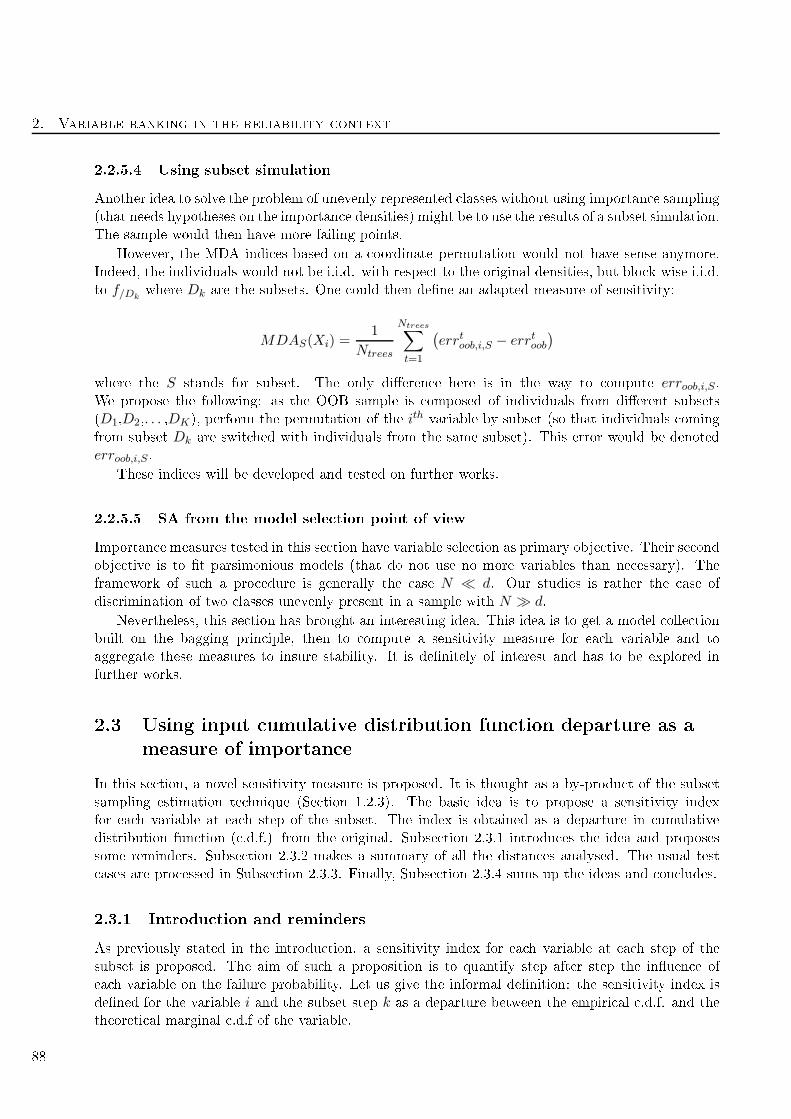
2. Variable ranking in the reliability ontext
2.2.5.4 Using subset simulation
Another idea to solve the problem of unevenly represented lasses without using importan e sampling
(that needs hypotheses on the importan e densities) might be to use the results of a subset simulation.
The sample would then have more failing points.
However, the MDA indi es based on a oordinate permutation would not have sense anymore.
Indeed, the individuals would not be i.i.d. with respe t to the original densities, but blo k-wise i.i.d.
to f/Dkwhere Dk are the subsets. One ould then dene an adapted measure of sensitivity:
MDAS(Xi) =1
Ntrees
Ntrees∑
t=1
(errtoob,i,S − errtoob
)
where the S stands for subset. The only dieren e here is in the way to ompute erroob,i,S.We propose the following: as the OOB sample is omposed of individuals from dierent subsets
(D1,D2,. . . ,DK), perform the permutation of the ith variable by subset (so that individuals oming
from subset Dk are swit hed with individuals from the same subset). This error would be denoted
erroob,i,S.
These indi es will be developed and tested on further works.
2.2.5.5 SA from the model sele tion point of view
Importan e measures tested in this se tion have variable sele tion as primary obje tive. Their se ond
obje tive is to t parsimonious models (that do not use no more variables than ne essary). The
framework of su h a pro edure is generally the ase N ≪ d. Our studies is rather the ase of
dis rimination of two lasses unevenly present in a sample with N ≫ d.
Nevertheless, this se tion has brought an interesting idea. This idea is to get a model olle tion
built on the bagging prin iple, then to ompute a sensitivity measure for ea h variable and to
aggregate these measures to insure stability. It is denitely of interest and has to be explored in
further works.
2.3 Using input umulative distribution fun tion departure as a
measure of importan e
In this se tion, a novel sensitivity measure is proposed. It is thought as a by-produ t of the subset
sampling estimation te hnique (Se tion 1.2.3). The basi idea is to propose a sensitivity index
for ea h variable at ea h step of the subset. The index is obtained as a departure in umulative
distribution fun tion ( .d.f.) from the original. Subse tion 2.3.1 introdu es the idea and proposes
some reminders. Subse tion 2.3.2 makes a summary of all the distan es analysed. The usual test
ases are pro essed in Subse tion 2.3.3. Finally, Subse tion 2.3.4 sums up the ideas and on ludes.
2.3.1 Introdu tion and reminders
As previously stated in the introdu tion, a sensitivity index for ea h variable at ea h step of the
subset is proposed. The aim of su h a proposition is to quantify step after step the inuen e of
ea h variable on the failure probability. Let us give the informal denition: the sensitivity index is
dened for the variable i and the subset step k as a departure between the empiri al .d.f. and the
theoreti al marginal .d.f of the variable.
88
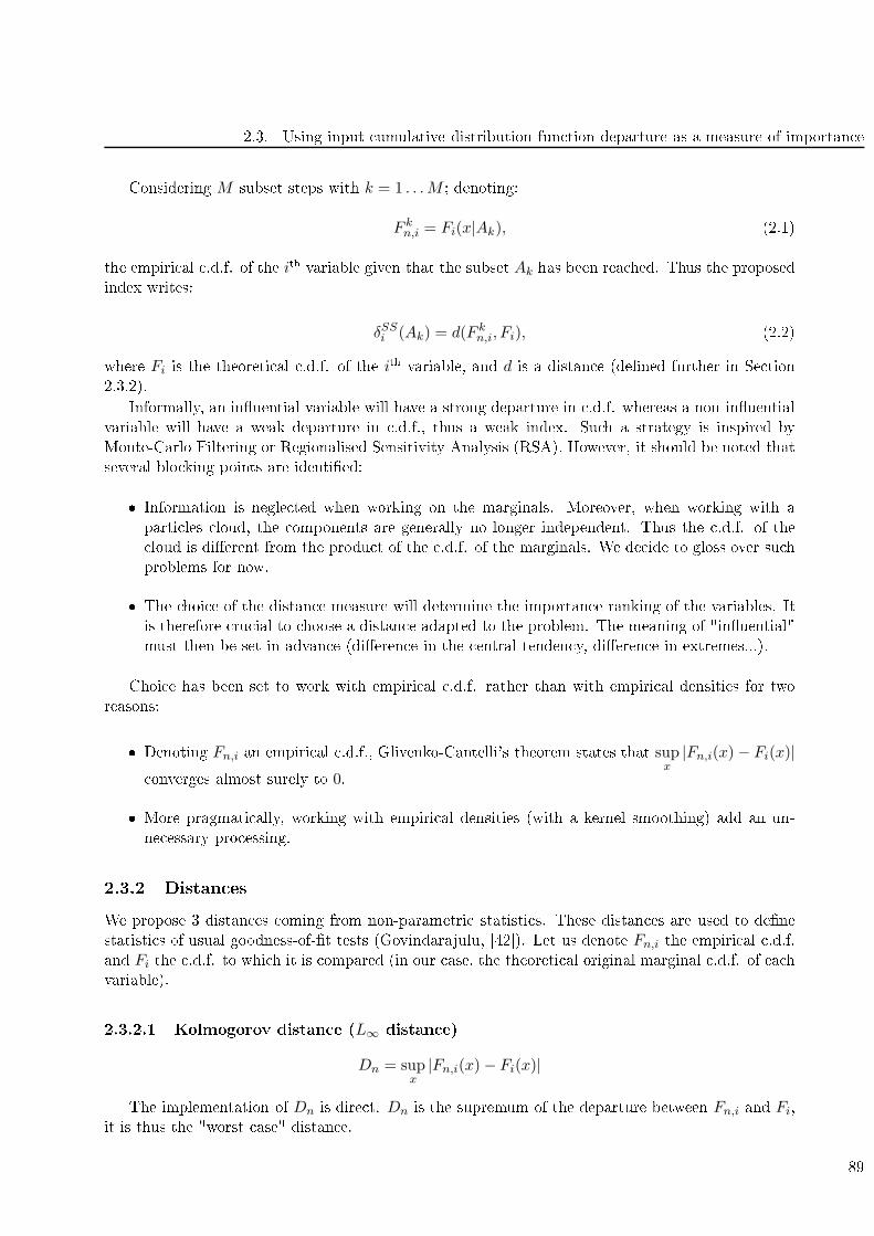
2.3. Using input umulative distribution fun tion departure as a measure of importan e
Considering M subset steps with k = 1 . . .M ; denoting:
F kn,i = Fi(x|Ak), (2.1)
the empiri al .d.f. of the ith variable given that the subset Ak has been rea hed. Thus the proposed
index writes:
δSSi (Ak) = d(F kn,i, Fi), (2.2)
where Fi is the theoreti al .d.f. of the ith
variable, and d is a distan e (dened further in Se tion
2.3.2).
Informally, an inuential variable will have a strong departure in .d.f. whereas a non-inuential
variable will have a weak departure in .d.f., thus a weak index. Su h a strategy is inspired by
Monte-Carlo Filtering or Regionalised Sensitivity Analysis (RSA). However, it should be noted that
several blo king points are identied:
Information is negle ted when working on the marginals. Moreover, when working with a
parti les loud, the omponents are generally no longer independent. Thus the .d.f. of the
loud is dierent from the produ t of the .d.f. of the marginals. We de ide to gloss over su h
problems for now.
The hoi e of the distan e measure will determine the importan e ranking of the variables. It
is therefore ru ial to hoose a distan e adapted to the problem. The meaning of "inuential"
must then be set in advan e (dieren e in the entral tenden y, dieren e in extremes...).
Choi e has been set to work with empiri al .d.f. rather than with empiri al densities for two
reasons:
Denoting Fn,i an empiri al .d.f., Glivenko-Cantelli's theorem states that supx
|Fn,i(x)− Fi(x)| onverges almost surely to 0.
More pragmati ally, working with empiri al densities (with a kernel smoothing) add an un-
ne essary pro essing.
2.3.2 Distan es
We propose 3 distan es oming from non-parametri statisti s. These distan es are used to dene
statisti s of usual goodness-of-t tests (Govindarajulu, [42). Let us denote Fn,i the empiri al .d.f.
and Fi the .d.f. to whi h it is ompared (in our ase, the theoreti al original marginal .d.f. of ea h
variable).
2.3.2.1 Kolmogorov distan e (L∞ distan e)
Dn = supx
|Fn,i(x)− Fi(x)|
The implementation of Dn is dire t. Dn is the supremum of the departure between Fn,i and Fi,
it is thus the "worst ase" distan e.
89
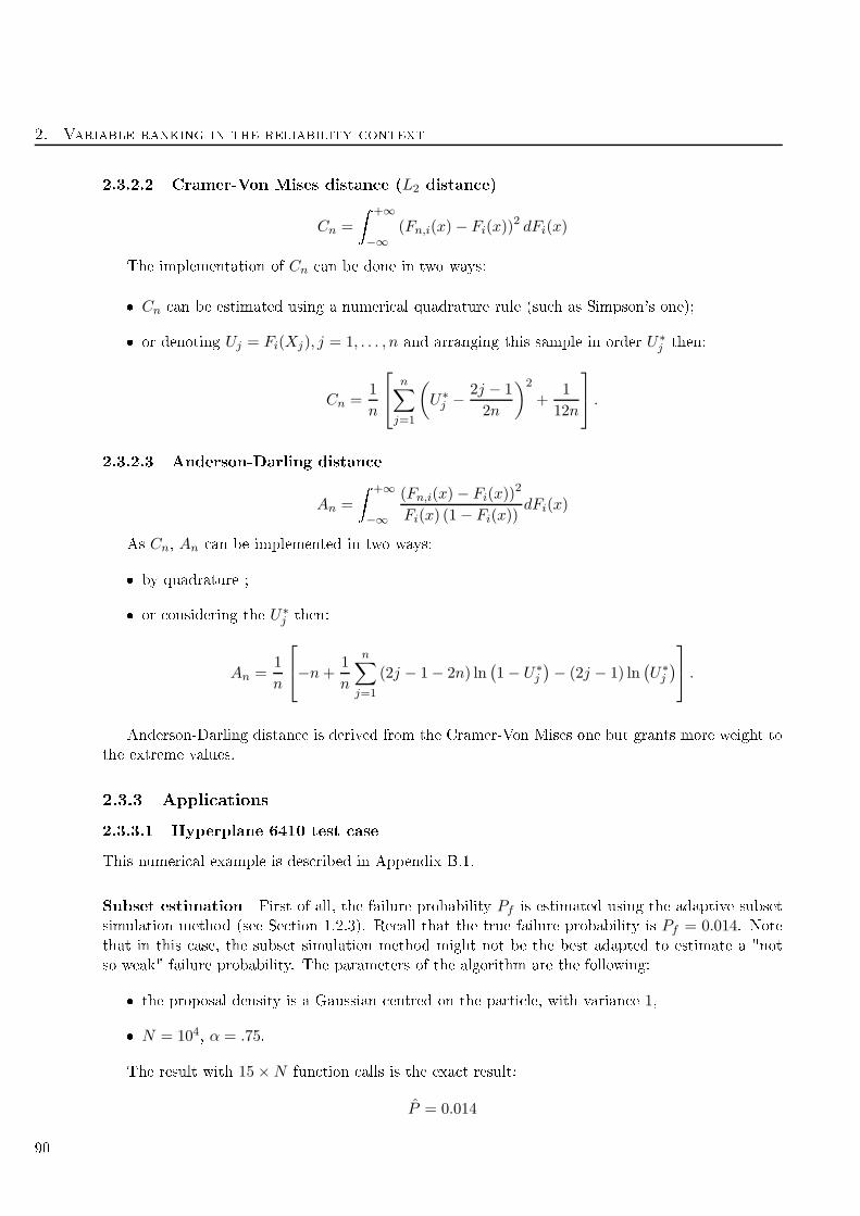
2. Variable ranking in the reliability ontext
2.3.2.2 Cramer-Von Mises distan e (L2 distan e)
Cn =
+∞
−∞(Fn,i(x)− Fi(x))
2 dFi(x)
The implementation of Cn an be done in two ways:
Cn an be estimated using a numeri al quadrature rule (su h as Simpson's one);
or denoting Uj = Fi(Xj), j = 1, . . . , n and arranging this sample in order U∗j then:
Cn =1
n
n∑
j=1
(U∗j − 2j − 1
2n
)2
+1
12n
.
2.3.2.3 Anderson-Darling distan e
An =
+∞
−∞
(Fn,i(x)− Fi(x))2
Fi(x) (1− Fi(x))dFi(x)
As Cn, An an be implemented in two ways:
by quadrature ;
or onsidering the U∗j then:
An =1
n
−n+
1
n
n∑
j=1
(2j − 1− 2n) ln(1− U∗
j
)− (2j − 1) ln
(U∗j
) .
Anderson-Darling distan e is derived from the Cramer-Von Mises one but grants more weight to
the extreme values.
2.3.3 Appli ations
2.3.3.1 Hyperplane 6410 test ase
This numeri al example is des ribed in Appendix B.1.
Subset estimation First of all, the failure probability Pf is estimated using the adaptive subset
simulation method (see Se tion 1.2.3). Re all that the true failure probability is Pf = 0.014. Notethat in this ase, the subset simulation method might not be the best adapted to estimate a "not
so weak" failure probability. The parameters of the algorithm are the following:
the proposal density is a Gaussian entred on the parti le, with varian e 1,
N = 104, α = .75.
The result with 15×N fun tion alls is the exa t result:
P = 0.014
90

2.3. Using input umulative distribution fun tion departure as a measure of importan e
Plot of the .d.f. For this rst example, the .d.f given that the third, the seventh and the
fteenth subset have been rea hed are plotted in Figure 2.9. One an see that whatever the distan e
used, the .d.f. orresponding to the fteenth subset is farther from the original one that the .d.f.
orresponding to the third subset (on this example).
−4 −2 0 2 4
0.0
0.2
0.4
0.6
0.8
1.0
x
Fn(x)
Fi
Fn,i(x A3)
Fn,i(x A7)
Fn,i(x A15)
Figure 2.9: Several .d.f.
Distan e estimation The distan e are estimated with the formulas given in 2.3.2. They are
plotted in fun tion of the threshold in Figures 2.10, 2.11 and 2.12. Variable X1 is plotted in bla k,
X2 in blue, X3 in green and X4 in red.
91

2. Variable ranking in the reliability ontext
0.0
0.2
0.4
0.6
0.8
Threshold
Kol
mog
orov
dis
tanc
e
21.0 17.2 14.5 12.5 10.8 9.2 6.7 4.4 2.5 0.6
Figure 2.10: Hyperplane 6410 test ase, Kolmogorov distan e
0.00
0.05
0.10
0.15
0.20
0.25
Threshold
Cra
mer
−V
on M
ises
dis
tanc
e
21.0 17.2 14.5 12.5 10.8 9.2 6.7 4.4 2.5 0.6
Figure 2.11: Hyperplane 6410 test ase, Cramer-Von Mises distan e
92

2.3. Using input umulative distribution fun tion departure as a measure of importan e
0.0
0.5
1.0
1.5
2.0
Threshold
And
erso
n−D
arlin
g di
stan
ce
21.0 17.2 14.5 12.5 10.8 9.2 6.7 4.4 2.5 0.6
Figure 2.12: Hyperplane 6410 test ase, Anderson-Darling distan e
All the distan es allow the following variable ranking: X2,X3,X1 then X4. Noti e that this is
the same ranking tan the one provided by the importan e fa tors (see Table 3.3). All the distan es
tend to separate the variables in two groups. The Anderson-Darling distan e seems to minimise the
inuen e of the rst variable (bla k).
2.3.3.2 Hyperplane 11111 test ase
This numeri al example is des ribed in Appendix B.1. Re all that the aim of this test ase is to
assess the apability of the SA method to give the same importan e to ea h input.
Subset estimation The failure probability Pf is estimated using the adaptive subset simulation
method (see Se tion 1.2.3). Re all that the true failure probability is Pf = 0.0036. The algorithm's
parameters are the following:
the proposal density is a Gaussian entred on the parti le, with varian e 1,
N = 104, α = .75.
The result with 20×N fun tion alls is the exa t result:
P = 0.0036
Distan e estimation The distan es are estimated with the formulas given in 2.3.2. They are
plotted in fun tion of the threshold in Figures 2.13, 2.14 and 2.15. A dierent olor is used for ea h
variable.
93
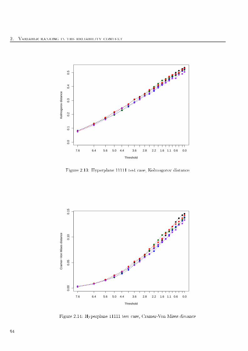
2. Variable ranking in the reliability ontext
0.0
0.1
0.2
0.3
0.4
0.5
Threshold
Kol
mog
orov
dis
tanc
e
7.6 6.4 5.6 5.0 4.4 3.6 2.8 2.2 1.6 1.1 0.6 0.0
Figure 2.13: Hyperplane 11111 test ase, Kolmogorov distan e
0.00
0.05
0.10
0.15
Threshold
Cra
mer
−V
on M
ises
dis
tanc
e
7.6 6.4 5.6 5.0 4.4 3.6 2.8 2.2 1.6 1.1 0.6 0.0
Figure 2.14: Hyperplane 11111 test ase, Cramer-Von Mises distan e
94
2.3. Using input umulative distribution fun tion departure as a measure of importan e
0.0
0.2
0.4
0.6
0.8
Threshold
And
erso
n−D
arlin
g di
stan
ce
7.6 6.4 5.6 5.0 4.4 3.6 2.8 2.2 1.6 1.1 0.6 0.0
Figure 2.15: Hyperplane 11111 test ase, Anderson-Darling distan e
Every distan e gives to the 5 variables the same importan e. The distan es growth with the
threshold. So far, this SA method has proven that it an give the same inuen e to equally inuential
variables.
2.3.3.3 Hyperplane 15 variables test ase
This numeri al example is des ribed in Appendix B.1. Re all that the aim of this test ase is to
lass the inputs in 3 groups: inuential, weakly-inuential and non-inuential.
Subset estimation The failure probability Pf is estimated using the adaptive subset simulation
method (see Se tion 1.2.3). Re all that the true failure probability is Pf = 0.00425. The algorithm's
parameters are the following:
the proposal density is a Gaussian entred on the parti le, with varian e 1,
N = 104, α = .75.
The result with 19×N fun tion alls is lose from the exa t result:
P = 0.00454
Distan e estimation The distan es are estimated with the formulas given in 2.3.2. They are
plotted in fun tion of the threshold in Figures 2.16, 2.17 and 2.18. A dierent olor is used for ea h
variable. A dierent symbol (respe tively a dot, a triangle and a square) is used for ea h group
(respe tively inuential, weakly-inuential and non-inuential).
95
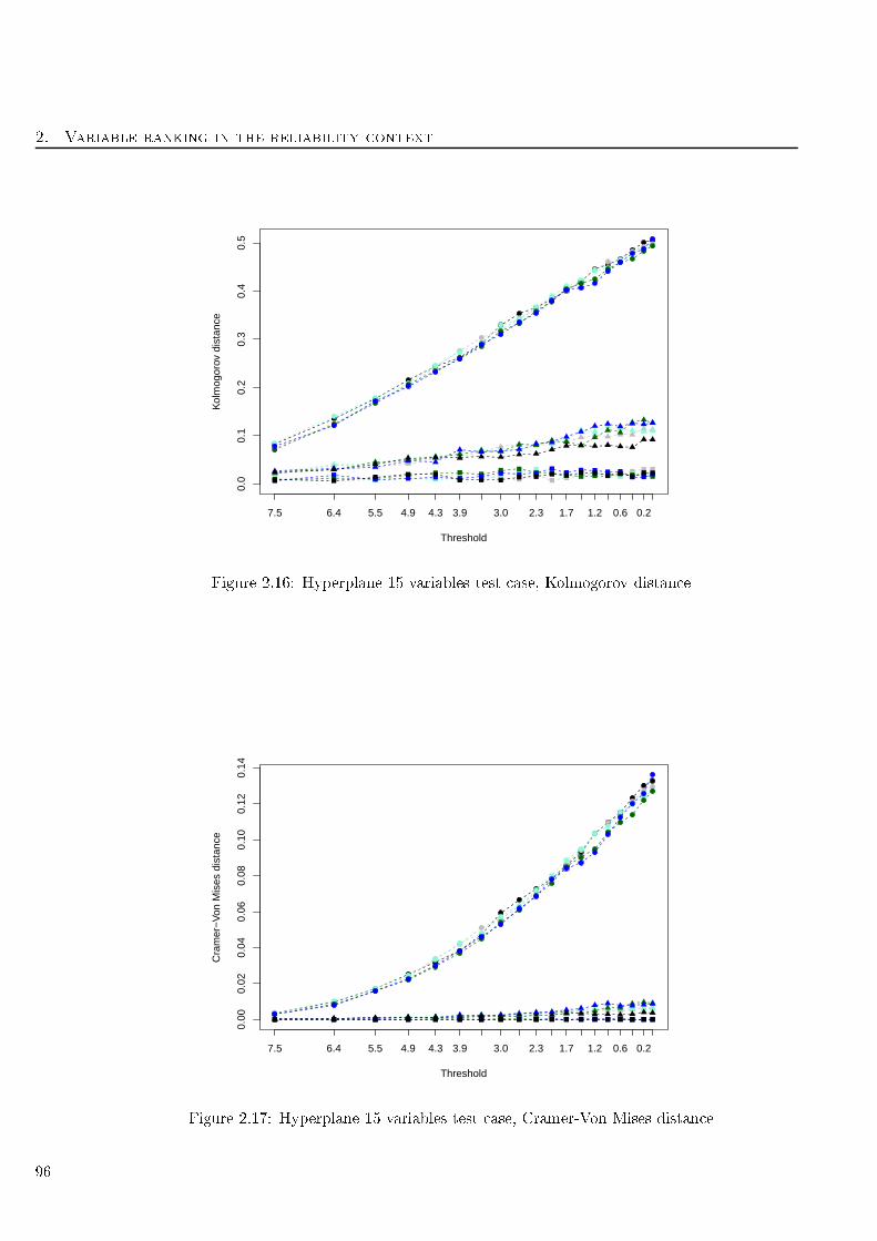
2. Variable ranking in the reliability ontext
0.0
0.1
0.2
0.3
0.4
0.5
Threshold
Kol
mog
orov
dis
tanc
e
7.5 6.4 5.5 4.9 4.3 3.9 3.0 2.3 1.7 1.2 0.6 0.2
Figure 2.16: Hyperplane 15 variables test ase, Kolmogorov distan e
0.00
0.02
0.04
0.06
0.08
0.10
0.12
0.14
Threshold
Cra
mer
−V
on M
ises
dis
tanc
e
7.5 6.4 5.5 4.9 4.3 3.9 3.0 2.3 1.7 1.2 0.6 0.2
Figure 2.17: Hyperplane 15 variables test ase, Cramer-Von Mises distan e
96
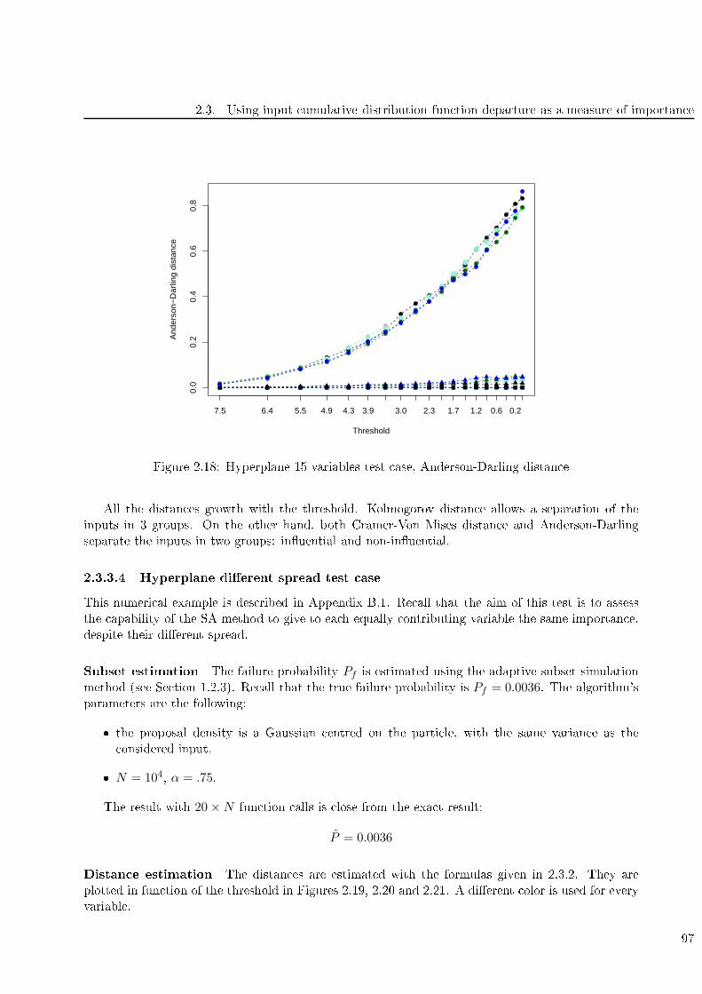
2.3. Using input umulative distribution fun tion departure as a measure of importan e
0.0
0.2
0.4
0.6
0.8
Threshold
And
erso
n−D
arlin
g di
stan
ce
7.5 6.4 5.5 4.9 4.3 3.9 3.0 2.3 1.7 1.2 0.6 0.2
Figure 2.18: Hyperplane 15 variables test ase, Anderson-Darling distan e
All the distan es growth with the threshold. Kolmogorov distan e allows a separation of the
inputs in 3 groups. On the other hand, both Cramer-Von Mises distan e and Anderson-Darling
separate the inputs in two groups: inuential and non-inuential.
2.3.3.4 Hyperplane dierent spread test ase
This numeri al example is des ribed in Appendix B.1. Re all that the aim of this test is to assess
the apability of the SA method to give to ea h equally ontributing variable the same importan e,
despite their dierent spread.
Subset estimation The failure probability Pf is estimated using the adaptive subset simulation
method (see Se tion 1.2.3). Re all that the true failure probability is Pf = 0.0036. The algorithm's
parameters are the following:
the proposal density is a Gaussian entred on the parti le, with the same varian e as the
onsidered input,
N = 104, α = .75.
The result with 20×N fun tion alls is lose from the exa t result:
P = 0.0036
Distan e estimation The distan es are estimated with the formulas given in 2.3.2. They are
plotted in fun tion of the threshold in Figures 2.19, 2.20 and 2.21. A dierent olor is used for every
variable.
97
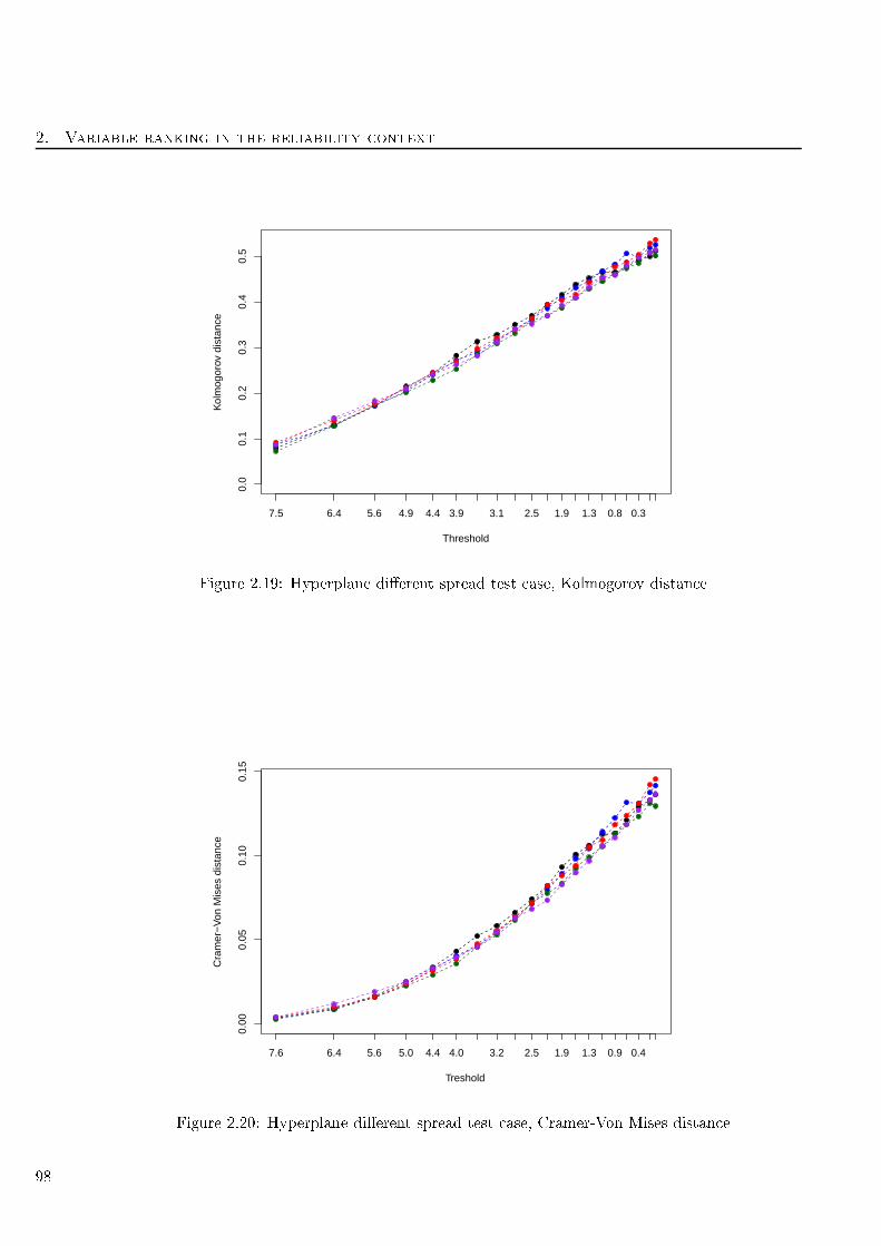
2. Variable ranking in the reliability ontext
0.0
0.1
0.2
0.3
0.4
0.5
Threshold
Kol
mog
orov
dis
tanc
e
7.5 6.4 5.6 4.9 4.4 3.9 3.1 2.5 1.9 1.3 0.8 0.3
Figure 2.19: Hyperplane dierent spread test ase, Kolmogorov distan e
0.00
0.05
0.10
0.15
Treshold
Cra
mer
−V
on M
ises
dis
tanc
e
7.6 6.4 5.6 5.0 4.4 4.0 3.2 2.5 1.9 1.3 0.9 0.4
Figure 2.20: Hyperplane dierent spread test ase, Cramer-Von Mises distan e
98
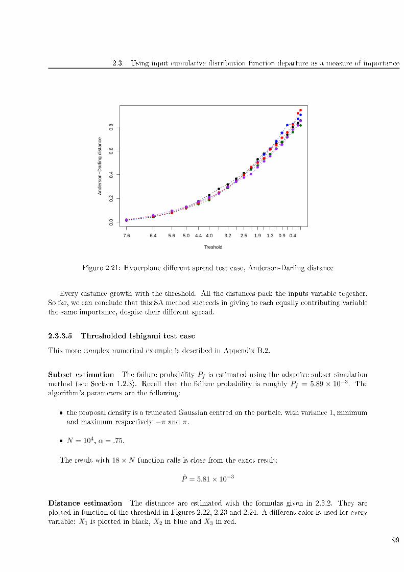
2.3. Using input umulative distribution fun tion departure as a measure of importan e
0.0
0.2
0.4
0.6
0.8
Treshold
And
erso
n−D
arlin
g di
stan
ce
7.6 6.4 5.6 5.0 4.4 4.0 3.2 2.5 1.9 1.3 0.9 0.4
Figure 2.21: Hyperplane dierent spread test ase, Anderson-Darling distan e
Every distan e growth with the threshold. All the distan es pa k the inputs variable together.
So far, we an on lude that this SA method su eeds in giving to ea h equally ontributing variable
the same importan e, despite their dierent spread.
2.3.3.5 Thresholded Ishigami test ase
This more omplex numeri al example is des ribed in Appendix B.2.
Subset estimation The failure probability Pf is estimated using the adaptive subset simulation
method (see Se tion 1.2.3). Re all that the failure probability is roughly Pf = 5.89 × 10⁻³. The
algorithm's parameters are the following:
the proposal density is a trun ated Gaussian entred on the parti le, with varian e 1, minimum
and maximum respe tively −π and π,
N = 104, α = .75.
The result with 18×N fun tion alls is lose from the exa t result:
P = 5.81 × 10⁻³
Distan e estimation The distan es are estimated with the formulas given in 2.3.2. They are
plotted in fun tion of the threshold in Figures 2.22, 2.23 and 2.24. A dierent olor is used for every
variable: X1 is plotted in bla k, X2 in blue and X3 in red.
99

2. Variable ranking in the reliability ontext
0.0
0.1
0.2
0.3
0.4
0.5
0.6
Threshold
Kol
mog
orov
dis
tanc
e
13.0 11.2 9.7 8.5 7.2 6.2 5.1 3.6 2.2 1.0 0.0
Figure 2.22: Thresholded Ishigami test ase, Kolmogorov distan e
0.00
0.02
0.04
0.06
0.08
0.10
0.12
Threshold
Cra
mer
−V
on M
ises
dis
tanc
e
13.0 11.2 9.7 8.5 7.2 6.2 5.1 3.6 2.2 1.0 0.0
Figure 2.23: Thresholded Ishigami test ase, Cramer-Von Mises distan e
100
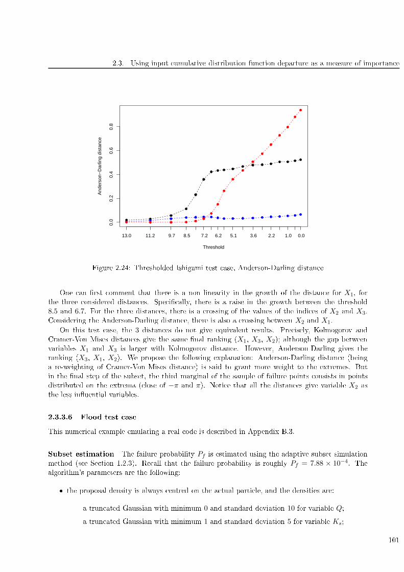
2.3. Using input umulative distribution fun tion departure as a measure of importan e
0.0
0.2
0.4
0.6
0.8
Threshold
And
erso
n−D
arlin
g di
stan
ce
13.0 11.2 9.7 8.5 7.2 6.2 5.1 3.6 2.2 1.0 0.0
Figure 2.24: Thresholded Ishigami test ase, Anderson-Darling distan e
One an rst omment that there is a non linearity in the growth of the distan e for X1, for
the three onsidered distan es. Spe i ally, there is a raise in the growth between the threshold
8.5 and 6.7. For the three distan es, there is a rossing of the values of the indi es of X2 and X3.
Considering the Anderson-Darling distan e, there is also a rossing between X2 and X1.
On this test ase, the 3 distan es do not give equivalent results. Pre isely, Kolmogorov and
Cramer-Von Mises distan es give the same nal ranking (X1, X3, X2); although the gap between
variables X1 and X3 is larger with Kolmogorov distan e. However, Anderson-Darling gives the
ranking (X3, X1, X2). We propose the following explanation: Anderson-Darling distan e (being
a re-weighting of Cramer-Von Mises distan e) is said to grant more weight to the extremes. But
in the nal step of the subset, the third marginal of the sample of failure points onsists in points
distributed on the extrema ( lose of −π and π). Noti e that all the distan es give variable X2 as
the less inuential variables.
2.3.3.6 Flood test ase
This numeri al example emulating a real ode is des ribed in Appendix B.3.
Subset estimation The failure probability Pf is estimated using the adaptive subset simulation
method (see Se tion 1.2.3). Re all that the failure probability is roughly Pf = 7.88 × 10⁻⁴. The
algorithm's parameters are the following:
the proposal density is always entred on the a tual parti le, and the densities are:
a trun ated Gaussian with minimum 0 and standard deviation 10 for variable Q;
a trun ated Gaussian with minimum 1 and standard deviation 5 for variable Ks;
101
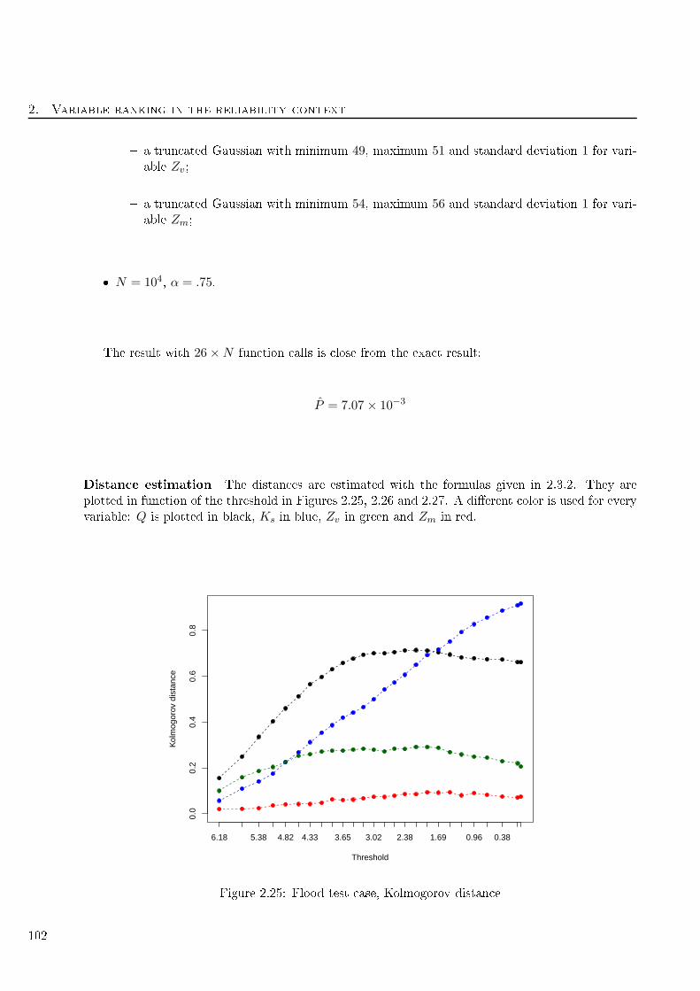
2. Variable ranking in the reliability ontext
a trun ated Gaussian with minimum 49, maximum 51 and standard deviation 1 for vari-
able Zv;
a trun ated Gaussian with minimum 54, maximum 56 and standard deviation 1 for vari-
able Zm;
N = 104, α = .75.
The result with 26×N fun tion alls is lose from the exa t result:
P = 7.07 × 10⁻³
Distan e estimation The distan es are estimated with the formulas given in 2.3.2. They are
plotted in fun tion of the threshold in Figures 2.25, 2.26 and 2.27. A dierent olor is used for every
variable: Q is plotted in bla k, Ks in blue, Zv in green and Zm in red.
0.0
0.2
0.4
0.6
0.8
Threshold
Kol
mog
orov
dis
tanc
e
6.18 5.38 4.82 4.33 3.65 3.02 2.38 1.69 0.96 0.38
Figure 2.25: Flood test ase, Kolmogorov distan e
102
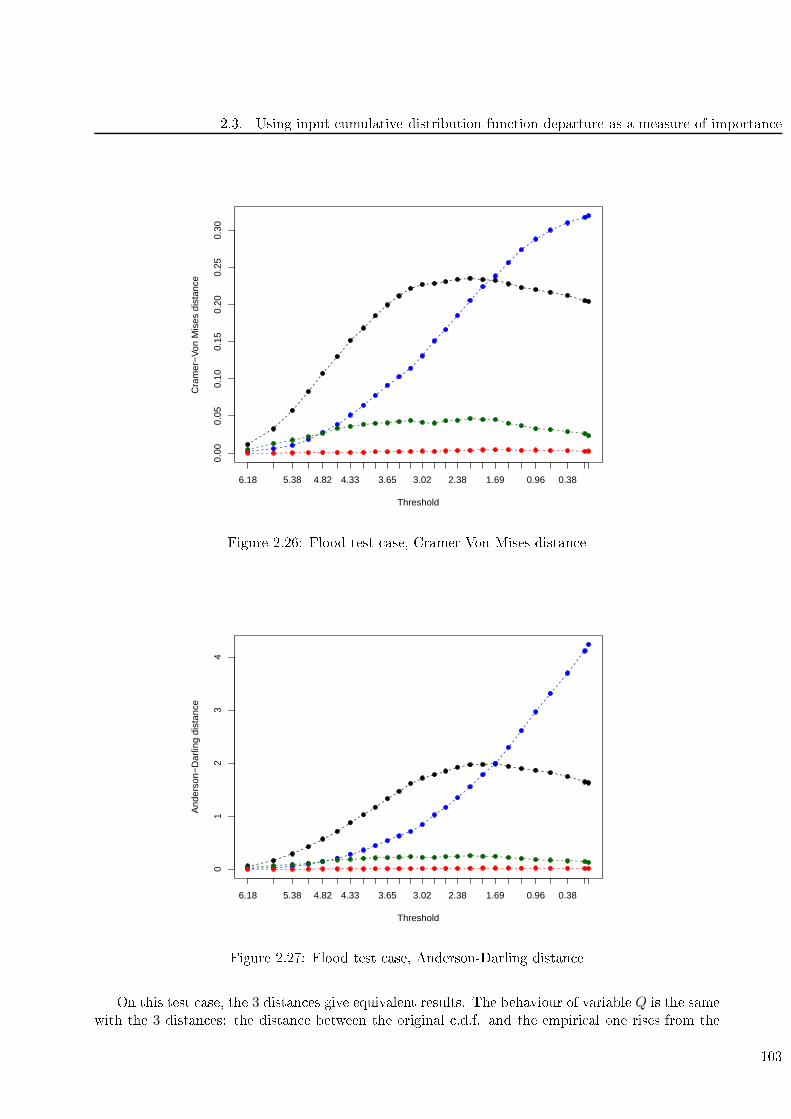
2.3. Using input umulative distribution fun tion departure as a measure of importan e
0.00
0.05
0.10
0.15
0.20
0.25
0.30
Threshold
Cra
mer
−V
on M
ises
dis
tanc
e
6.18 5.38 4.82 4.33 3.65 3.02 2.38 1.69 0.96 0.38
Figure 2.26: Flood test ase, Cramer-Von Mises distan e
01
23
4
Threshold
And
erso
n−D
arlin
g di
stan
ce
6.18 5.38 4.82 4.33 3.65 3.02 2.38 1.69 0.96 0.38
Figure 2.27: Flood test ase, Anderson-Darling distan e
On this test ase, the 3 distan es give equivalent results. The behaviour of variable Q is the same
with the 3 distan es: the distan e between the original .d.f. and the empiri al one rises from the
103

2. Variable ranking in the reliability ontext
beginning until the threshold rea hes 2. Then the distan e diminishes slowly. The behaviour is the
same for variable Zv although with mu h less amplitude. The distan e for variable Ks growths with
the subset. For variable Zm, the distan e stagnates around the minimal value. The nal ranking is
Ks, Q, Zv, Zm for the 3 distan es, whi h is the one provided by the importan e fa tors (see Table
3.16).
2.3.4 Con lusion
The proposed SA te hnique allows an use of the subset simulation methods. In parti ular, we
used adaptive levels algorithms.
The omputational time is negligible with respe t to the omputational time needed to obtain
the failure sample.
The three proposed distan es bring omplementary informations on the failure sample.
Kolmogorov distan e is an L∞ one. It expresses the maximal gap between the empiri al
.d.f. of the failure sample and the original distribution. As far as we have noti ed on
the examples, it seems the more dis riminant distan e (see Figure 2.16 for instan e).
Cramer-Von Mises distan e is an L2 one. The indi es produ ed using this distan e answer
the question "what is the input whi h distribution varies most in entral tenden y when
restri ted to the failure domain?". The use of su h a distan e is then re ommended if the
aim of the SA is to x the non-inuential input variables to their entral value.
Anderson-Darling distan e grants more weight to the extreme values. The indi es pro-
du ed using this distan e answer the question "what is the input whi h distribution varies
most in the extremes when restri ted to the failure domain?". The use of su h a distan e
is re ommended when the aim of the SA is to determine the relative inuen e of the
boundaries or extremes of input distributions.
So far, this SA method is re ommended to get a similar information as the one provided by the
Sobol' indi es on the failure indi ator (that is to say the dete tion of variables less inuential
than others).
However, this method provides an interesting additional information: it shows how the thresh-
old impa ts ea h variable. This is interesting in the sense that, in some real ases, the threshold
might not be xed by the physi s but by the regulation. A threshold given for a safety study
might not be the same for another study. This method has shown (on the Ishigami test ase)
that the ranking might be dierent for several threshold ( rossing of the urves between X2
and X3 for instan e).
2.4 Synthesis
This hapter has presented two SA methods provide a variable ranking (obje tive 1, REM1, see
Se tion 1.7). A rst part was devoted to lassi ation methods for SA, with a spe ial attention paid
to random forests. A se ond part was devoted to measuring the departure between the original and
the empiri al .d.f. at several steps of a subset simulation method.
Table 2.10 is a short synthesis on the SA methods presented throughout this hapter.
104
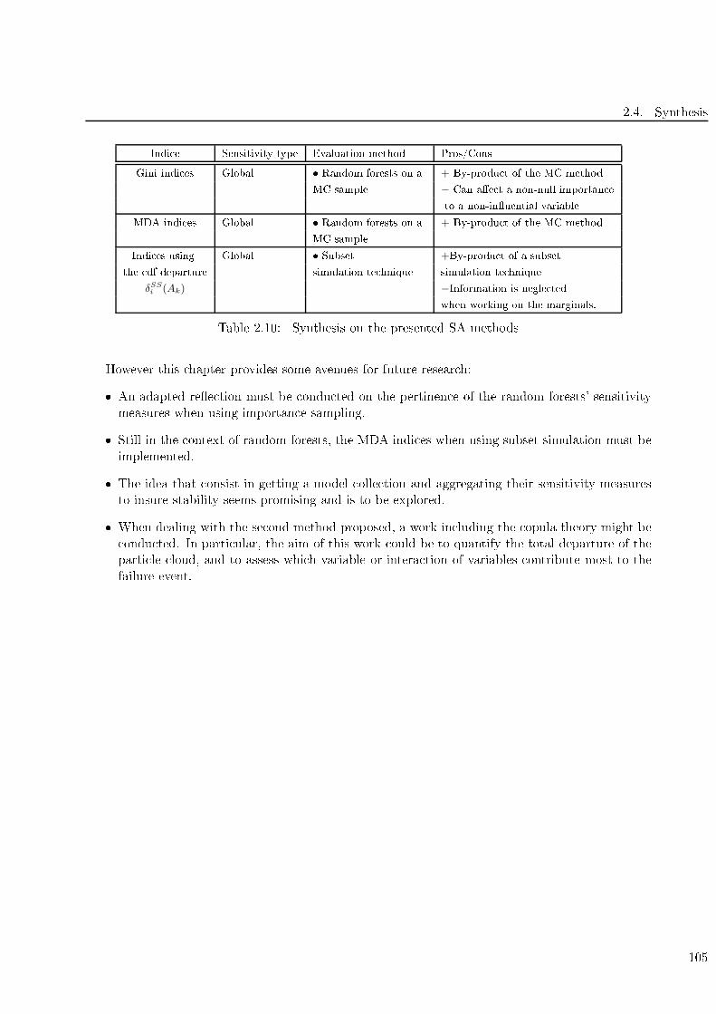
2.4. Synthesis
Indi e Sensitivity type Evaluation method Pros/Cons
Gini indi es Global Random forests on a + By-produ t of the MC method
MC sample − Can ae t a non-null importan e
to a non-inuential variable
MDA indi es Global Random forests on a + By-produ t of the MC method
MC sample
Indi es using Global Subset +By-produ t of a subset
the df departure simulation te hnique simulation te hnique
δSSi (Ak) −Information is negle ted
when working on the marginals.
Table 2.10: Synthesis on the presented SA methods
However this hapter provides some avenues for future resear h:
An adapted ree tion must be ondu ted on the pertinen e of the random forests' sensitivity
measures when using importan e sampling.
Still in the ontext of random forests, the MDA indi es when using subset simulation must be
implemented.
The idea that onsist in getting a model olle tion and aggregating their sensitivity measures
to insure stability seems promising and is to be explored.
When dealing with the se ond method proposed, a work in luding the opula theory might be
ondu ted. In parti ular, the aim of this work ould be to quantify the total departure of the
parti le loud, and to assess whi h variable or intera tion of variables ontribute most to the
failure event.
105


Chapter 3
Density Modi ation Based Reliability
Sensitivity Indi es
3.1 Introdu tion and overview
In most studies, sensitivity indi es for failure probabilities are dened in strong orresponden e with
a given method of estimation (e.g. Lemaire [61, Munoz Zuniga et al. [73). Their interpretation
is onsequently limited. In this hapter, it is proposed to dene new generi sensitivity reliability
indi es. Our sensitivity index is based upon input density modi ation, and is adapted to failure
probabilities. A methodology to estimate su h indi es is derived.
The proposed indi es ree t the impa t of the input density modi ation on the failure prob-
ability Pf . The indi es are independent of the perturbation in the sense that the pra titioner an
set the perturbation adapted to his/her problem. Dierent modi ations/perturbations will answer
dierent problems.
For simpli ity reasons, a lassi al Monte Carlo framework is onsidered in the following, although
the estimation pro ess will be extended to the use of subset and importan e sampling methods. The
sensitivity index an be omputed using the sole set of simulations that has already been used to
estimate the failure probability Pf , thus limiting the number of alls to the numeri al model, as
spe ied in the onstraints of the CWNR ase (page 24)
The outline of this hapter is the following: rst, the indi es and their theoreti al properties are
presented in Se tion 3.2, altogether with the estimation methodology. Se ond, Se tion 3.3 deals with
several perturbation methodologies. These perturbations an be lassied into two main families:
Kullba k-Leibler minimization methods and parameter perturbations methods. The behaviour of
the indi es is examined in Se tion 3.4 through numeri al simulations in various omplexity settings
(see Appendix B). Comparisons with two referen e sensitivity analysis methods (FORM's impor-
tan e fa tors and Sobol' indi es, see Se tion 1.3) highlight the relevan e of the new indi es in most
situations. In Se tion 3.5, it is proposed to improve the DMBRSI estimation with importan e sam-
pling and with subset simulation. The main advantages and remaining issues are nally dis ussed
in the last se tion of the hapter, that introdu es avenues for future resear h.
This hapter is the extended version of the paper [63.
107
3. Density Modifi ation Based Reliability Sensitivity Indi es
3.2 The indi es: denition, properties and estimation
3.2.1 Denition
Given a unidimensional input variable Xi with pdf fi, let us all Xiδ ∼ fiδ the orresponding
perturbed random input. This perturbed input takes the pla e of the real random input Xi, in
a sense of modelling error : what if the orre t input were Xiδ instead of Xi? More about this
repla ement is proposed thereafter, see Se tion 3.3.1.1. Re all that we onsider that (X1, . . . ,Xd)are mutually independent.
The perturbed failure probability be omes:
Piδ =
1G(x)<0fiδ(xi)
fi(xi)f(x)dx (3.1)
where xi is the ith omponent of the ve tor x. Independently of the me hanism hosen for the
perturbation (see next se tion for proposals), a good sensitivity index Siδ should have intuitive
features that make it appealing to reliability engineers and de ision-makers. We argue that the
following denition an fulll these requirements.
Denition 3.2.1 Dene the Density Modi ation Based Reliability Sensitivity Indi es (DMBRSI)
as the quantity Siδ:
Siδ =
[Piδ
Pf− 1
]1Piδ≥Pf +
[1− Pf
Piδ
]1Piδ<Pf =
Piδ − Pf
Pf · 1Piδ≥Pf + Piδ · 1Piδ<Pf.
3.2.2 Properties
Firstly, Siδ = 0 if Piδ = Pf , as expe ted if Xi is a non-inuential variable or if δ expresses a
negligible perturbation.
Se ondly, the sign of Siδ indi ates how the perturbation impa ts the failure probability qualita-
tively. It highlights the situations when Piδ > Pf i.e. if the remaining (epistemi ) un ertainty
on the modelling Xi ∼ fi an in rease the failure risk. In this ase, the un ertainty on the
on erned variable should be more a urately analysed. Conversely, if Piδ < Pf , Pf an be
interpreted as a onservative assessment of the failure probability, with respe t to variations
of Xi. In su h a ase, deeper modelling studies on Xi appear less essential.
Thirdly, given its sign, the absolute value of Siδ has simple interpretation and provides a level
of the onservatism or non- onservatism indu ed by the perturbation. A value of α > 0 for
the index means that Piδ = (1 + α)Pf . If Siδ = −α < 0 then Piδ = (1/(1 + |α|))Pf .
3.2.3 Estimation
The postulated ability of Siδ to enlighten the sensitivity of P to input perturbations must be tested
in on rete ases (see Se tion 3.4), when an estimator PN of Pf an be omputed using an already
available design of N numeri al experiments. In the following, N is assumed to be large enough su h
that statisti al estimation stands within the framework of asymptoti theory. Besides, a standard
Monte Carlo design of experiments is assumed for simpli ity (see Se tion 1.2.1). This allows to write:
PN =1
N
N∑
n=1
1G(xn)<0
108
3.2. The indi es: denition, properties and estimation
where the x1, · · · ,xNare independent realisations of X. The strong Law of Large Numbers (LLN)
and the Central Limit Theorem (CLT) ensure that for almost all realisations PN −−−−→N→∞
Pf and
√N
Pf (1− Pf )(PN − Pf )
L−−−−→N→∞
N (0, 1). (3.2)
The Monte Carlo framework allows Piδ to be onsistently estimated without new alls to G, througha "reverse" importan e sampling me hanism:
PiδN =1
N
N∑
n=1
1G(xn)<0fiδ(x
ni )
fi(xni ). (3.3)
This property holds in the more general ase when P is originally estimated by importan e sampling
rather than simple Monte Carlo, whi h is more appealing when G is time- onsuming, Be kman and
M Key, Hesterberg [8, 45. This generalization is dis ussed further in the text (Se tion 3.5). The
following lemma ensures the asymptoti behaviour of su h an estimator.
Lemma 3.2.1 Assume the usual onditions
(i) Supp(fiδ) ⊆ Supp(fi),
(ii)
Supp(fi)
f2iδ(x)
fi(x)dx <∞,
then PiδN −−−−→N→∞
Piδ and
√Nσ−1
iδN
(PiδN − Piδ
) L−−−−→N→∞
N (0, 1). The exa t expression of σ−1iδN is
given in Appendix D.1, equation (D.1). It an be onsistently estimated by
σ2iδN =1
N
N∑
n=1
1G(xn)<0
(fiδ(x
ni )
fi(xni )
)2
− P 2iδN .
The proof of this Lemma is given in Appendix D.1.
We stress that Equation 3.3 is valid as long as the assumptions of Lemma 3.2.1 are respe ted.
This means that whatever the perturbation hosen, the estimation of PiδN does not require new
fun tion alls.
The asymptoti properties of any estimator of Siδ will depend on the orrelation between PN
and PiδN . The next proposition summarizes the features of the joint asymptoti distribution of both
estimators.
Proposition 3.2.1 Under assumptions (i) and (ii) of Lemma 3.2.1,
√N
[(PN
PiδN
)−(Pf
Piδ
)]L−−−−→
N→∞N2 (0,Σiδ)
where Σiδ is given in Appendix D.1, Equation (D.2) and an be onsistently estimated by
Σiδ =
(PN (1− PN ) PiδN (1− PN )
PiδN (1− PN ) σ2iδN
).
The proof of this Proposition is given in Appendix D.1.
109
3. Density Modifi ation Based Reliability Sensitivity Indi es
Given (PN , PiδN ), the plugging estimator for Siδ is:
SiδN =
[PiδN
PN
− 1
]1PiδN≥PN +
[1− PN
PiδN
]1PiδN<PN. (3.4)
In orollary of Proposition 3.2.1, applying the ontinuous-mapping theorem to the fun tion s(x, y) =[ yx − 1
]1y≥x+
[1− x
y
]1y<x, SiδN onverges almost surely to Siδ. The following CLT results from
Theorem 3.1 in Van der Vaart [98.
Proposition 3.2.2 Assume that assumptions (i) and (ii) of Lemma 3.2.1 hold and further that
P 6= Piδ, we have
√N[S
iδN − Siδ
] L−−−−→N→∞
N(0, dTs Σds
)(3.5)
with ds =
(∂s
∂x(Pf , Piδ),
∂s
∂y(Pf , Piδ)
)T
for x 6= y, and
∂s
∂x(x, y) = −y1y≥x/x
2 − 1
y1y<x,
∂s
∂y(x, y) =
1
x1y≥x + x1y<x/y
2.
This holds when Pf = Piδ. Indeed, one has for x∗ 6= 0 :
limy ≥ x
(
x
y
)
→
(
x∗
y∗
)
∇s(x, y) = limy < x
(
x
y
)
→
(
x∗
y∗
)
∇s(x, y) =(− 1
x∗,1
x∗
)T
.
3.2.4 Framework
Figure 3.1 summarises the use of DMBRSI.
110

3.2. The indi es: denition, properties and estimation
Get a MC sample
x1, · · · ,xN ∼ f
Dene a spe i
perturbation
(see Se tion 3.3)
i = 1..d
Set perturbation
parameter δ within a
given variation range
Get an expression of fiδ
Estimate the
quantities:
PiδN (see Eq. (3.3))
SiδN (see Eq. (3.4))
Σiδ (see Prop. 3.2.1)
Plot SiδN in fun tion of δPlot onden e intervals
around SiδN from dTs Σds
While in the variation
range, hange δ
If i < d, i = i+ 1
End
Figure 3.1: General DMBRSI framework
111

3. Density Modifi ation Based Reliability Sensitivity Indi es
The notion of perturbation is dis ussed in the next se tion. Whi h perturbation to hoose
a ording to the obje tive is also dis ussed as well as re ommendations on the variation range of δ.
3.3 Methodologies of input perturbation
This se tion proposes several perturbation methodologies. However the DMBRSI and its estimation
te hniques remain valid for any perturbation, as long as the support onstraints (Lemma 3.2.1) are
respe ted. Here, two main families of method are presented. The rst one determines the perturbed
density minimizing the Kullba k-Leibler divergen e under some onstraints given by the pra titioner.
Several onstraints are proposed, ea h one dealing with a dierent SA obje tive. The se ond method
is to be used when the pra titioner wants to test the sensitivity of Pf to the parameters of the
distributions. Both subse tions will be introdu ed by toy-examples.
This se tion illustrates the DMBRSI's apa ity to deal with several SA obje tives. The pra -
titioner is invited to propose new perturbation methodologies that would answer his questions.
Re ommendations of perturbation regarding the obje tives are itemized at the end of the se tion.
3.3.1 Kullba k-Leibler minimization
The DMBRSI requires to dene a perturbation for ea h input. In general, and espe ially in prelim-
inary reliability studies, there is no prior rule allowing to eli it a spe ialized perturbation for ea h
input variable. Thus a simple perturbation methodology is exposed -denoted KLM for Kullba k-
Leibler minimization- allowing the pra titioner to answer the questions itemized in Se tion 1.7 of
the present thesis.
3.3.1.1 First example
Let us assume we have an input Xi distributed a ording to fi. This random input models for
instan e a physi al un ertain quantity. The distribution fi is known, altogether with its parameters.
This modelling was done by physi expert, engineers, pra titioners, statisti al analyst from eld
data ... Moments of Xi are also known given they exist.
We would like to fairly perturb this input to represent "the la k of ertitude" on some quantity.
This quantity might be, as a simple example, the rst moment. Let us assume the input Xi is
distributed a ording to a Gaussian, N (0, 1). What if the expe tation of Xi was badly modelled?
What if the data used to alibrate fi were wrong?
We will thus suppose the existen e of another random variable Xiδ (distributed a ording to fiδ), lose from Xi in some sense, and we will pro ess it through the model, as if input Xi was repla ed
by the perturbed input Xiδ. δ represents here the perturbation, its amplitude for instan e.
Thus the example is an expe tation perturbation. What if the mean of the perturbed input were
2? New data an lead to su h a situation. So we want the new input to have:
E[Xiδ] = 2, (3.6)
obviously
fiδ(x)dx = 1 (3.7)
and Xiδ must be lose in some sense to Xi. Noti e that Equation (3.6) rewrites
xfiδ(x)dx = 2. (3.8)
112

3.3. Methodologies of input perturbation
−2 0 2 4 6 8 10
0.0
0.1
0.2
0.3
0.4
0.5
x
dens
ities
Figure 3.2: The original density of mean 0 (full line) and several andidates densities of mean 2
Several andidates for fiδ exist. In Figure 3.2 are plotted some hoi es, altogether with the
original density. Some andidates are " loser" to fi than others in some sense not yet dened. Let
us now fo us on the needs. We would like to take fiδ as the density, among all the densities satisfying
the onstraints (in our example, onstraint (3.6)), that is the minimum argument of a departure Dbetween densities.
fiδ = argmin
fmod
| onstraints holds
D(fmod
, fi) (3.9)
Distan e quantifying the departure between two densities are numerous (Cha [24). Information-
theoreti al arguments (Cover and Thomas [25) led to hoose the Kullba k-Leibler divergen e (KLD)
between fiδ and fi as a measure of the dis repan y to minimize under onstraints (denition of KLD
is reminded in 3.10). This omes at "adding" as few information as possible on fiδ other than the
onstraints.
By simple al ulus, it may be shown that the density minimizing the KLD from fi and satisfying
onstraints 3.6 is a Gaussian, of mean 2 and of the same varian e as fi. The omputation of the
indi es expressed in Se tion Se tion 3.2 an now be done as fiδ is provided.
Next subse tion formalises this example.
3.3.1.2 Kullba k-Leibler minimization
Here, a perturbed input density fiδ is dened as the losest distribution to the original fi in the
entropi sense and under some onstraints of perturbation.
113
3. Density Modifi ation Based Reliability Sensitivity Indi es
Later (see Se tions 3.3.1.3, 3.3.1.4), spe i perturbations orresponding to a mean shift, a
varian e shift and a quantile shift will be presented.
Re all that between two pdf p and q we have:
KL(p, q) =
+∞
−∞p(y) log
p(y)
q(y)dy if log
p(y)
q(y)∈ L1(p(y)dy). (3.10)
Let i = 1, · · · , d, the onstraints are expressed as follows in fun tion of the modied density fmod
:
gk(xi)fmod
(xi)dxi = δk,i (k = 1 · · ·K) . (3.11)
Here, for k = 1, · · · ,K, gk are given fun tions and δk,i are given real. These quantities will lead
to a perturbation of the original density. The modied density fiδ onsidered in our work is:
fiδ = argmin
fmod
|(3.11) holds
KL(fmod
, fi) (3.12)
and the result takes an expli it form (Csiszar, [26) given in the following proposition.
Proposition 3.3.1 Let us dene, for λ = (λ1, · · · , λK)T ∈ RK,
ψi(λ) = log
fi(x) exp
[K∑
k=1
λkgk(x)
]dx , (3.13)
where the last integral an be nite or innite (in this last ase ψi(λ) = +∞). Further, set Dom ψi =λ ∈ RK |ψi(λ) < +∞. Assume that there exists at least one pdf f
mod
satisfying (3.11) and that
Dom ψi is an open set. Then, there exists a unique λ∗su h that the solution of the minimisation
problem (3.12) is
fiδ(xi) = fi(xi) exp
[K∑
k=1
λ∗kgk(xi)− ψi(λ∗)
]. (3.14)
The theoreti al te hnique to ompute λ is provided in Appendix D.2.
3.3.1.3 Moments shifting
Mean shifting The rst moment is often used to parametrize a distribution. Thus the rst
perturbation presented here is a mean shift, that is expressed with a single onstraint:
xifmod
(xi)dxi = δi . (3.15)
In terms of SA, this perturbation should be used when the user wants to understand the sensi-
tivity of the inputs to a mean shift - that is to say "what if the mean of input Xi were δi insteadof E [Xi]?". Noti e that for most distributions, this amounts to testing the sensitivity to the entral
tenden y.
Proposition 3.3.2 Considering onstraint (3.15), under the assumptions of Proposition 3.3.1, the
expression of the optimal perturbed density is
fiδi(xi) = exp(λ∗xi − ψi(λ∗))fi(xi) (3.16)
where λ∗ is su h that Equation (3.15) holds.
114
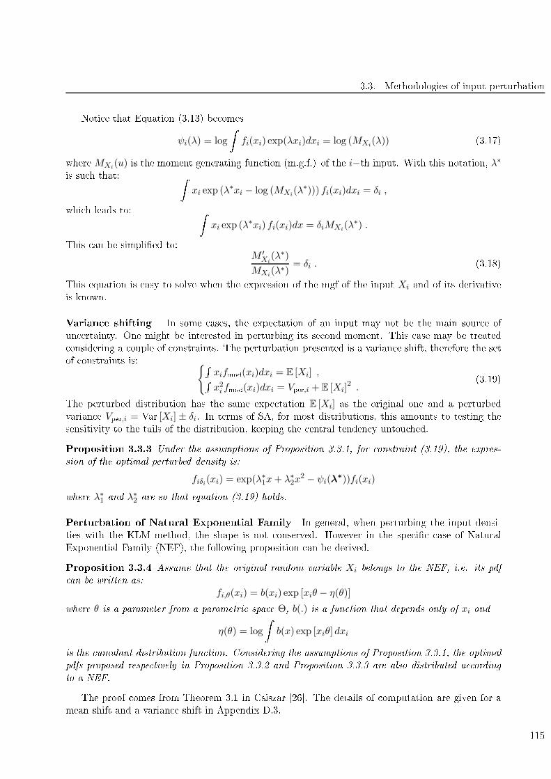
3.3. Methodologies of input perturbation
Noti e that Equation (3.13) be omes
ψi(λ) = log
fi(xi) exp(λxi)dxi = log (MXi(λ)) (3.17)
where MXi(u) is the moment generating fun tion (m.g.f.) of the i−th input. With this notation, λ∗
is su h that:
xi exp (λ∗xi − log (MXi
(λ∗))) fi(xi)dxi = δi ,
whi h leads to:
xi exp (λ∗xi) fi(xi)dx = δiMXi
(λ∗) .
This an be simplied to:
M ′Xi(λ∗)
MXi(λ∗)
= δi . (3.18)
This equation is easy to solve when the expression of the mgf of the input Xi and of its derivative
is known.
Varian e shifting In some ases, the expe tation of an input may not be the main sour e of
un ertainty. One might be interested in perturbing its se ond moment. This ase may be treated
onsidering a ouple of onstraints. The perturbation presented is a varian e shift, therefore the set
of onstraints is:
xifmod
(xi)dxi = E [Xi] ,
x2i fmod
(xi)dxi = Vper,i + E [Xi]
2 .(3.19)
The perturbed distribution has the same expe tation E [Xi] as the original one and a perturbed
varian e Vper,i = Var [Xi] ± δi. In terms of SA, for most distributions, this amounts to testing the
sensitivity to the tails of the distribution, keeping the entral tenden y untou hed.
Proposition 3.3.3 Under the assumptions of Proposition 3.3.1, for onstraint (3.19), the expres-
sion of the optimal perturbed density is:
fiδi(xi) = exp(λ∗1x+ λ∗2x2 − ψi(λ
∗))fi(xi)
where λ∗1 and λ∗2 are so that equation (3.19) holds.
Perturbation of Natural Exponential Family In general, when perturbing the input densi-
ties with the KLM method, the shape is not onserved. However in the spe i ase of Natural
Exponential Family (NEF), the following proposition an be derived.
Proposition 3.3.4 Assume that the original random variable Xi belongs to the NEF, i.e. its pdf
an be written as:
fi,θ(xi) = b(xi) exp [xiθ − η(θ)]
where θ is a parameter from a parametri spa e Θ, b(.) is a fun tion that depends only of xi and
η(θ) = log
b(x) exp [xiθ]dxi
is the umulant distribution fun tion. Considering the assumptions of Proposition 3.3.1, the optimal
pdfs proposed respe tively in Proposition 3.3.2 and Proposition 3.3.3 are also distributed a ording
to a NEF.
The proof omes from Theorem 3.1 in Csiszar [26. The details of omputation are given for a
mean shift and a varian e shift in Appendix D.3.
115

3. Density Modifi ation Based Reliability Sensitivity Indi es
Some shapes As an example, the two kinds of perturbations previously presented are provided
for two families of inputs (Gaussian and Uniform) in Figure 3.3. The perturbations are respe tively
a mean and varian e in reasing. It is noti eable (as proven in Proposition 3.3.4) that the shape is
onserved for the Gaussian distribution when shifting the mean or the varian e. On the other hand,
when in reasing its mean, the Uniform distribution is pa ked down on the right-hand boundary of
its support. When in reasing its varian e, the density is pa ked down on both boundaries of its
support.
Figure 3.3: Mean shifting (left) and varian e shifting (right) for Gaussian (upper) and Uniform
(lower) distributions. The original distribution is plotted in solid line, the perturbed one is plotted
in dashed line.
Some limitations, notion of equivalent perturbation In this paragraph, we fo us on a mean
shift but the same problems arise for a varian e shift. What if two inputs do not have the same
mean and we want to assess the impa t of their mean shift on Pf? How to ondu t an equivalent
perturbation on both inputs? Let us imagine an example in whi h an input has mean 0 and another
has mean 100. If a perturbation is ondu ted on ea h variable separately, the interpretation is
ompli ated as the ranges of variation will be separated. It is thus ompli ated or impossible to
assess the impa t of an equivalent perturbation. Conversely, it is impossible in this ase to make
a "relative mean shift" as one of the input has mean 0. The following solution is proposed for the
mean perturbation: shift the mean relatively to the standard deviation, hen e in luding the spread
of the various inputs in their respe tive perturbation. So for any input, the original distribution
116

3.3. Methodologies of input perturbation
is perturbed so that its mean is the original's one plus δ times its standard deviation and the
perturbation is ondu ted on δ (for instan e ranging from −1 to 1). This solution is applied in
the ood ase (Se tion 3.4.7) where the inputs are not distributed a ording to the same density.
However this solution might not be ee tive in every ase, for instan e when inputs do not have
dened moments. This onsideration led us to another kind of perturbation that we though is
more equivalent: quantile shifting (see Se tion 3.3.1.4). Moreover in the following of this thesis, the
perturbation will be ondu ted on the parameters of the input densities (see Se tion 3.3.2) but this
falls outside of the KLM framework.
3.3.1.4 Quantile shifting
Based on the pra titioner's experien e, it has been noti ed that the values of the input leading to the
failure event seldom lies around the entral tenden y, but more in the extreme quantiles. From this
point, another way to perturb the densities is proposed, keeping the KLM framework. Compared to
the rst two moment perturbations previously presented, we argue that this one seems more suitable
to deal with inputs that are not identi ally distributed (see previous paragraph for a dis ussion on
equivalent perturbations).
First example Let us rst re all the denition of a quantile.
Denition 3.3.1 For a given random variable X of probability density fun tion f and of umulative
distribution fun tion F , the α-quantile is the value qα so that:
P (X < qα) = F (qα) =
qα
−∞f(x)dx = α (3.20)
Then onsider a random variable, modelling for instan e an unknown physi al phenomena value,
dened as a standard Gaussian. Its 5% quantile or 5th per entile is q5% = −1.64.
As far as we noti ed, in most ases, the values of the input leading to the failure event omes
from the tails of the input distributions. What if these tails were badly modelled? Therefore a
perturbation based on the quantiles is proposed.
In this rst toy example, the aim is to in rease the weight of the left tail. That is to say that
the value q5% is wished to be ome for the modied density, for instan e the 7% quantile. This an
be written:
1]−∞;q5%](x)fmod
(x)dx = 7% (3.21)
In Figure 3.4 are plotted the regular (bla k) and the perturbed (blue) densities. The shaded
areas worth respe tively
q0.05−∞ f(x)dx = 0.05 in grey and
q0.05−∞ fδ(x)dx = 0.07 in blue. One an
remark that there is no longer a onservation of the shape with su h a perturbation, sin e fδ is notGaussian. Additionally, the density is no longer ontinuous.
In a similar way, one ould de ide to perturb the densities in su h a way that the tail is less
weighted, meaning that the extreme values be ome less frequent. For instan e, it an be written:
1]−∞;q5%](x)fmod
(x)dx = 3% (3.22)
meaning that the 5% quantile be omes the 3% quantile. The regular and the perturbed densities
are pi tured in Figure 3.4. A dis ontinuity at q5% is present.
117
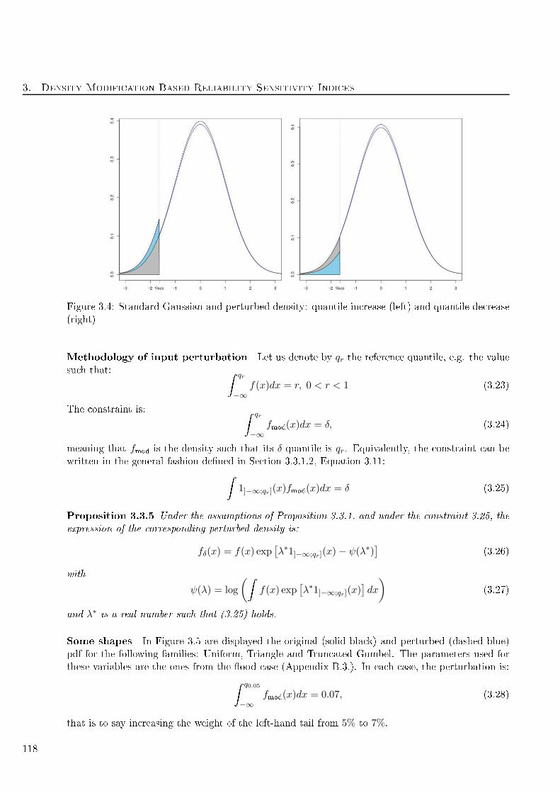
3. Density Modifi ation Based Reliability Sensitivity Indi es
Figure 3.4: Standard Gaussian and perturbed density: quantile in rease (left) and quantile de rease
(right)
Methodology of input perturbation Let us denote by qr the referen e quantile, e.g. the valuesu h that:
qr
−∞f(x)dx = r, 0 < r < 1 (3.23)
The onstraint is:
qr
−∞fmod
(x)dx = δ, (3.24)
meaning that fmod
is the density su h that its δ-quantile is qr. Equivalently, the onstraint an be
written in the general fashion dened in Se tion 3.3.1.2, Equation 3.11:
1]−∞;qr](x)fmod
(x)dx = δ (3.25)
Proposition 3.3.5 Under the assumptions of Proposition 3.3.1, and under the onstraint 3.25, the
expression of the orresponding perturbed density is:
fδ(x) = f(x) exp[λ∗1]−∞;qr](x)− ψ(λ∗)
](3.26)
with
ψ(λ) = log
(
f(x) exp[λ∗1]−∞;qr](x)
]dx
)(3.27)
and λ∗ is a real number su h that (3.25) holds.
Some shapes In Figure 3.5 are displayed the original (solid bla k) and perturbed (dashed blue)
pdf for the following families: Uniform, Triangle and Trun ated Gumbel. The parameters used for
these variables are the ones from the ood ase (Appendix B.3.). In ea h ase, the perturbation is:
q0.05
−∞fmod
(x)dx = 0.07, (3.28)
that is to say in reasing the weight of the left-hand tail from 5% to 7%.
118
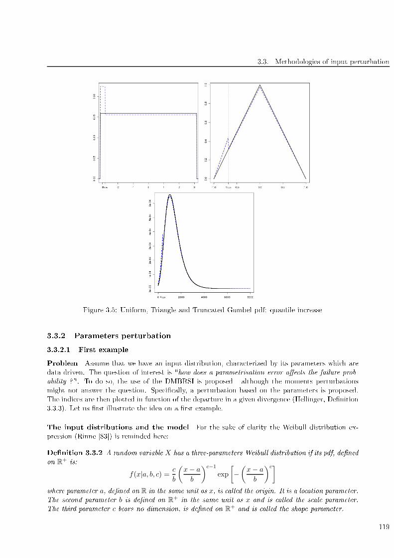
3.3. Methodologies of input perturbation
Figure 3.5: Uniform, Triangle and Trun ated Gumbel pdf: quantile in rease
3.3.2 Parameters perturbation
3.3.2.1 First example
Problem Assume that we have an input distribution, hara terized by its parameters whi h are
data-driven. The question of interest is "how does a parametrisation error ae ts the failure prob-
ability ?". To do so, the use of the DMBRSI is proposed - although the moments perturbations
might not answer the question. Spe i ally, a perturbation based on the parameters is proposed.
The indi es are then plotted in fun tion of the departure in a given divergen e (Hellinger, Denition
3.3.3). Let us rst illustrate the idea on a rst example.
The input distributions and the model For the sake of larity the Weibull distribution ex-
pression (Rinne [83) is reminded here:
Denition 3.3.2 A random variable X has a three-parameters Weibull distribution if its pdf, dened
on R+is:
f(x|a, b, c) = c
b
(x− a
b
)c−1
exp
[−(x− a
b
)c]
where parameter a, dened on R in the same unit as x, is alled the origin. It is a lo ation parameter.
The se ond parameter b is dened on R+in the same unit as x and is alled the s ale parameter.
The third parameter c bears no dimension, is dened on R+and is alled the shape parameter.
119
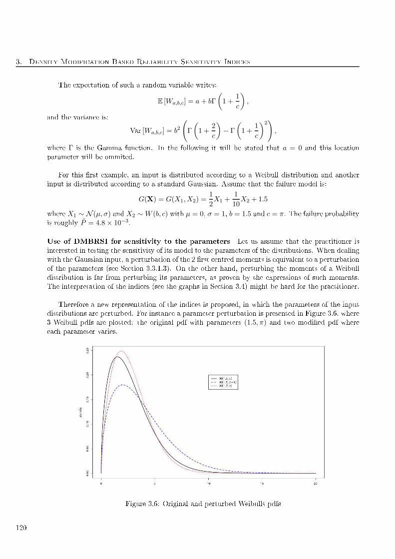
3. Density Modifi ation Based Reliability Sensitivity Indi es
The expe tation of su h a random variable writes:
E [Wa,b,c] = a+ bΓ
(1 +
1
c
),
and the varian e is:
Var [Wa,b,c] = b2
(Γ
(1 +
2
c
)− Γ
(1 +
1
c
)2),
where Γ is the Gamma fun tion. In the following it will be stated that a = 0 and this lo ation
parameter will be ommited.
For this rst example, an input is distributed a ording to a Weibull distribution and another
input is distributed a ording to a standard Gaussian. Assume that the failure model is:
G(X) = G(X1,X2) =1
2X1 +
1
10X2 + 1.5
where X1 ∼ N (µ, σ) and X2 ∼W (b, c) with µ = 0, σ = 1, b = 1.5 and c = π. The failure probabilityis roughly P = 4.8× 10⁻³
.
Use of DMBRSI for sensitivity to the parameters Let us assume that the pra titioner is
interested in testing the sensitivity of its model to the parameters of the distributions. When dealing
with the Gaussian input, a perturbation of the 2 rst entred moments is equivalent to a perturbation
of the parameters (see Se tion 3.3.1.3). On the other hand, perturbing the moments of a Weibull
distribution is far from perturbing its parameters, as proven by the expressions of su h moments.
The interpretation of the indi es (see the graphs in Se tion 3.4) might be hard for the pra titioner.
Therefore a new representation of the indi es is proposed, in whi h the parameters of the input
distributions are perturbed. For instan e a parameter perturbation is presented in Figure 3.6, where
3 Weibull pdfs are plotted: the original pdf with parameters (1.5, π) and two modied pdf where
ea h parameter varies.
Figure 3.6: Original and perturbed Weibulls pdfs
120
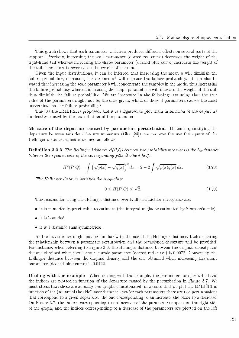
3.3. Methodologies of input perturbation
This graph shows that ea h parameter variation produ es dierent ee ts on several parts of the
support. Pre isely, in reasing the s ale parameter (dotted red urve) de reases the weight of the
right-hand tail whereas in reasing the shape parameter (dashed blue urve) in reases the weight of
the tail. The ee t is reversed on the weight of the mode.
Given the input distributions, it an be inferred that in reasing the mean µ will diminish the
failure probability, in reasing the varian e σ2 will in rease the failure probability. It an also be
stated that in reasing the s ale parameter b will on entrate the samples in the mode, thus in reasing
the failure probability whereas in reasing the shape parameter c will in rease the weight of the tail,thus diminish the failure probability. We are interested in the following: assuming that the true
value of the parameters might not be the ones given, whi h of those 4 parameters auses the most
un ertainty on the failure probability?
The use the DMBRSI is proposed, and it is suggested to plot them in fun tion of the departure
in density aused by the perturbation of the parameter.
Measure of the departure aused by parameters perturbation Distan e quantifying the
departure between two densities are numerous (Cha [24), we propose the use the square of the
Hellinger distan e, whi h is dened as follows.
Denition 3.3.3 The Hellinger Distan e H(P,Q) between two probability measures is the L2-distan e
between the square roots of the orresponding pdfs (Pollard [80).
H2(P,Q) =
(√p(x)−
√q(x)
)2dx = 2− 2
√p(x)q(x) dx. (3.29)
The Hellinger distan e satises the inequality:
0 ≤ H(P,Q) ≤√2. (3.30)
The reasons for using the Hellinger distan e over Kullba k-Liebler divergen e are:
it is numeri ally pra ti able to estimate (the integral might be estimated by Simpson's rule);
it is bounded;
it is a distan e thus symmetri al.
As the pra titioner might not be familiar with the use of the Hellinger distan e, tables eli iting
the relationship between a parameter perturbation and the o asioned departure will be provided.
For instan e, when referring to Figure 3.6, the Hellinger distan e between the original density and
the one obtained when in reasing the s ale parameter (dotted red urve) is 0.0072. Conversely, theHellinger distan e between the original density and the one obtained when in reasing the shape
parameter (dashed blue urve) is 0.0422.
Dealing with the example When dealing with the example, the parameters are perturbed and
the indi es are plotted in fun tion of the departure aused by the perturbation in Figure 3.7. We
must stress that these are a tually two graphs on atenated, in a sense that we plot the DMBSRI in
fun tion of the (square of the) Hellinger distan e - yet for ea h parameters there are two perturbations
that orrespond to a given departure: the one orresponding to an in rease, the other to a de rease.
On Figure 3.7, the indi es orresponding to an in rease of the parameters appear on the right side
of the graph, and the indi es orresponding to a de rease of the parameters are plotted on the left
121
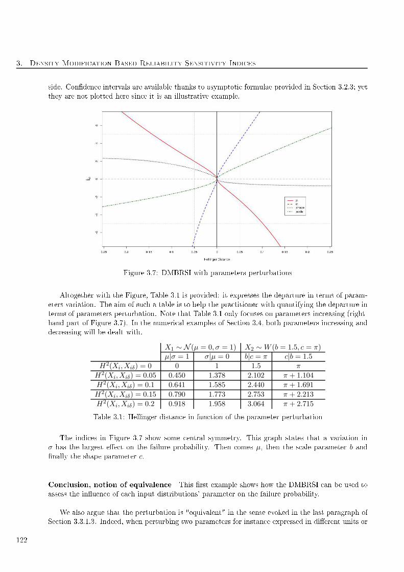
3. Density Modifi ation Based Reliability Sensitivity Indi es
side. Conden e intervals are available thanks to asymptoti formulae provided in Se tion 3.2.3; yet
they are not plotted here sin e it is an illustrative example.
Figure 3.7: DMBRSI with parameters perturbations
Altogether with the Figure, Table 3.1 is provided: it expresses the departure in terms of param-
eters variation. The aim of su h a table is to help the pra titioner with quantifying the departure in
terms of parameters perturbation. Note that Table 3.1 only fo uses on parameters in reasing (right-
hand part of Figure 3.7). In the numeri al examples of Se tion 3.4, both parameters in reasing and
de reasing will be dealt with.
X1 ∼ N (µ = 0, σ = 1) X2 ∼W (b = 1.5, c = π)µ|σ = 1 σ|µ = 0 b|c = π c|b = 1.5
H2(Xi,Xiδ) = 0 0 1 1.5 π
H2(Xi,Xiδ) = 0.05 0.450 1.378 2.102 π + 1.104
H2(Xi,Xiδ) = 0.1 0.641 1.585 2.440 π + 1.691
H2(Xi,Xiδ) = 0.15 0.790 1.773 2.753 π + 2.213
H2(Xi,Xiδ) = 0.2 0.918 1.958 3.064 π + 2.715
Table 3.1: Hellinger distan e in fun tion of the parameter perturbation
The indi es in Figure 3.7 show some entral symmetry. This graph states that a variation in
σ has the largest ee t on the failure probability. Then omes µ, then the s ale parameter b andnally the shape parameter c.
Con lusion, notion of equivalen e This rst example shows how the DMBRSI an be used to
assess the inuen e of ea h input distributions' parameter on the failure probability.
We also argue that the perturbation is "equivalent" in the sense evoked in the last paragraph of
Se tion 3.3.1.3. Indeed, when perturbing two parameters for instan e expressed in dierent units or
122
3.3. Methodologies of input perturbation
dierent orders of magnitude, the Hellinger distan e allows to quantify "equivalently" the amplitude
of the departure produ ed by the parameter shift.
3.3.2.2 Methodology of input perturbation
In this subse tion, we formalize what has been done in the previous rst example.
Let us suppose that the i-th variable Xi of the input ve tor is distributed a ording to fi. Thei-th input has pi parameters: it is parametrized by the ve tor Θi = (θi,1, .., θi,pi). The perturbationwill be on the j-th parameter, and will be of the following form:
θi,j,δ = θi,j + δi,j (3.31)
where δi,j is a given real su h that Θiδ = (θi,1, .., θi,j+δi,j, ., θi,pi) is still a parametrization ve tor
for the input fi (for instan e a varian e parameter annot be ome negative). Ve tor Θiδ parametrizes
the modied pdf fiδ. It must be noti ed as well that the support of the perturbed pdf fiδ must liewithin the support of fi (for estimation purposes, see onditions of Lemma 3.2.1).
The framework given in Figure 3.1 is modied in Figure 3.8 to onsider the parameters pertur-
bations.
123
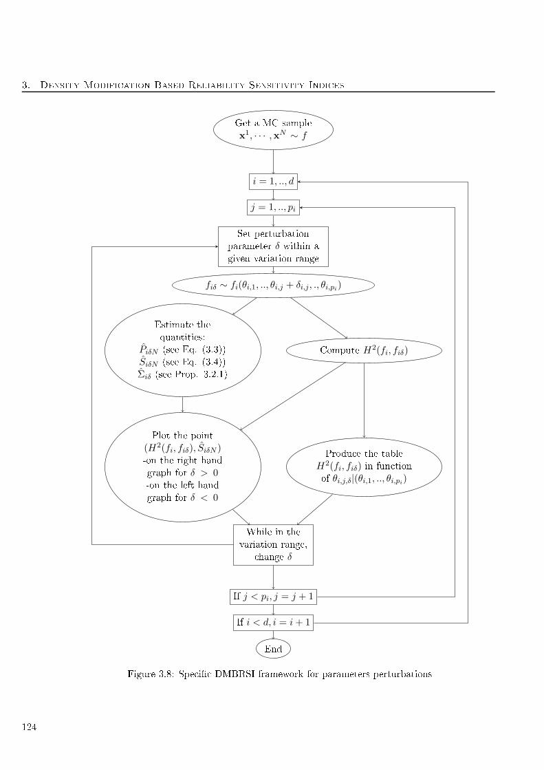
3. Density Modifi ation Based Reliability Sensitivity Indi es
Get a MC sample
x1, · · · ,xN ∼ f
i = 1, .., d
j = 1, .., pi
Set perturbation
parameter δ within a
given variation range
fiδ ∼ fi(θi,1, .., θi,j + δi,j, ., θi,pi)
Estimate the
quantities:
PiδN (see Eq. (3.3))
SiδN (see Eq. (3.4))
Σiδ (see Prop. 3.2.1)
Compute H2(fi, fiδ)
Plot the point
(H2(fi, fiδ), SiδN )-on the right hand
graph for δ > 0-on the left hand
graph for δ < 0
Produ e the table
H2(fi, fiδ) in fun tion
of θi,j,δ|(θi,1, .., θi,pi)
While in the
variation range,
hange δ
If i < d, i = i+ 1
If j < pi, j = j + 1
End
Figure 3.8: Spe i DMBRSI framework for parameters perturbations
124
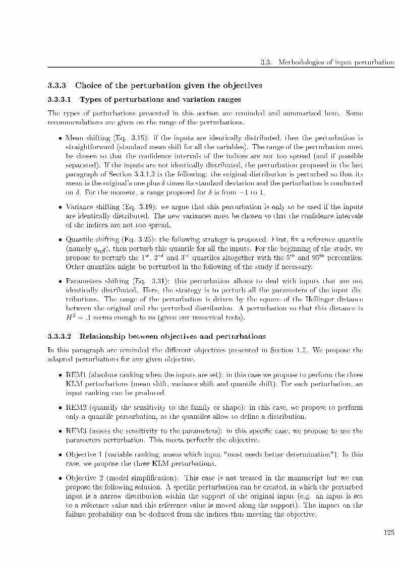
3.3. Methodologies of input perturbation
3.3.3 Choi e of the perturbation given the obje tives
3.3.3.1 Types of perturbations and variation ranges
The types of perturbations presented in this se tion are reminded and summarized here. Some
re ommendations are given on the range of the perturbations.
Mean shifting (Eq. 3.15): if the inputs are identi ally distributed, then the perturbation is
straightforward (standard mean shift for all the variables). The range of the perturbation must
be hosen so that the onden e intervals of the indi es are not too spread (and if possible
separated). If the inputs are not identi ally distributed, the perturbation proposed in the last
paragraph of Se tion 3.3.1.3 is the following: the original distribution is perturbed so that its
mean is the original's one plus δ times its standard deviation and the perturbation is ondu ted
on δ. For the moment, a range proposed for δ is from −1 to 1.
Varian e shifting (Eq. 3.19): we argue that this perturbation is only to be used if the inputs
are identi ally distributed. The new varian es must be hosen so that the onden e intervals
of the indi es are not too spread.
Quantile shifting (Eq. 3.25): the following strategy is proposed. First, x a referen e quantile
(namely qref
), then perturb this quantile for all the inputs. For the beginning of the study, we
propose to perturb the 1st, 2nd and 3rd quartiles altogether with the 5th and 95th per entiles.
Other quantiles might be perturbed in the following of the study if ne essary.
Parameters shifting (Eq. 3.31): this perturbation allows to deal with inputs that are not
identi ally distributed. Here, the strategy is to perturb all the parameters of the input dis-
tributions. The range of the perturbation is driven by the square of the Hellinger distan e
between the original and the perturbed distribution. A perturbation so that this distan e is
H2 = .1 seems enough to us (given our numeri al tests).
3.3.3.2 Relationship between obje tives and perturbations
In this paragraph are reminded the dierent obje tives presented in Se tion 1.7. We propose the
adapted perturbations for any given obje tive.
REM1 (absolute ranking when the inputs are set): in this ase we propose to perform the three
KLM perturbations (mean shift, varian e shift and quantile shift). For ea h perturbation, an
input ranking an be produ ed.
REM2 (quantify the sensitivity to the family or shape): in this ase, we propose to perform
only a quantile perturbation, as the quantiles allow to dene a distribution.
REM3 (assess the sensitivity to the parameters): in this spe i ase, we propose to use the
parameters perturbation. This meets perfe tly the obje tive.
Obje tive 1 (variable ranking, assess whi h input "most needs better determination"). In this
ase, we propose the three KLM perturbations.
Obje tive 2 (model simpli ation). This ase is not treated in the manus ript but we an
propose the following solution. A spe i perturbation an be reated, in whi h the perturbed
input is a narrow distribution within the support of the original input (e.g. an input is set
to a referen e value and this referen e value is moved along the support). The impa t on the
failure probability an be dedu ed from the indi es thus meeting the obje tive.
125
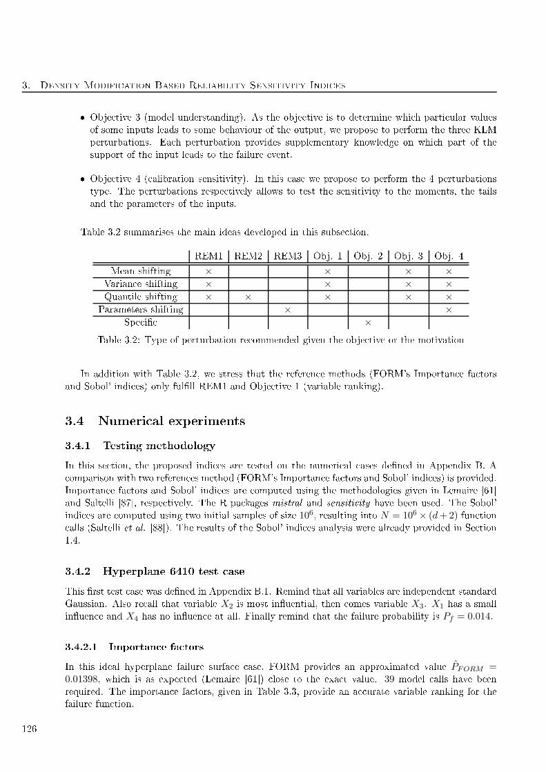
3. Density Modifi ation Based Reliability Sensitivity Indi es
Obje tive 3 (model understanding). As the obje tive is to determine whi h parti ular values
of some inputs leads to some behaviour of the output, we propose to perform the three KLM
perturbations. Ea h perturbation provides supplementary knowledge on whi h part of the
support of the input leads to the failure event.
Obje tive 4 ( alibration sensitivity). In this ase we propose to perform the 4 perturbations
type. The perturbations respe tively allows to test the sensitivity to the moments, the tails
and the parameters of the inputs.
Table 3.2 summarises the main ideas developed in this subse tion.
REM1 REM2 REM3 Obj. 1 Obj. 2 Obj. 3 Obj. 4
Mean shifting × × × ×Varian e shifting × × × ×Quantile shifting × × × × ×
Parameters shifting × ×Spe i ×
Table 3.2: Type of perturbation re ommended given the obje tive or the motivation
In addition with Table 3.2, we stress that the referen e methods (FORM's Importan e fa tors
and Sobol' indi es) only fulll REM1 and Obje tive 1 (variable ranking).
3.4 Numeri al experiments
3.4.1 Testing methodology
In this se tion, the proposed indi es are tested on the numeri al ases dened in Appendix B. A
omparison with two referen es method (FORM's Importan e fa tors and Sobol' indi es) is provided.
Importan e fa tors and Sobol' indi es are omputed using the methodologies given in Lemaire [61
and Saltelli [87, respe tively. The R pa kages mistral and sensitivity have been used. The Sobol'
indi es are omputed using two initial samples of size 106, resulting into N = 106 × (d+2) fun tion alls (Saltelli et al. [88). The results of the Sobol' indi es analysis were already provided in Se tion
1.4.
3.4.2 Hyperplane 6410 test ase
This rst test ase was dened in Appendix B.1. Remind that all variables are independent standard
Gaussian. Also re all that variable X2 is most inuential, then omes variable X3. X1 has a small
inuen e and X4 has no inuen e at all. Finally remind that the failure probability is Pf = 0.014.
3.4.2.1 Importan e fa tors
In this ideal hyperplane failure surfa e ase, FORM provides an approximated value PFORM =0.01398, whi h is as expe ted (Lemaire [61) lose to the exa t value. 39 model alls have been
required. The importan e fa tors, given in Table 3.3, provide an a urate variable ranking for the
failure fun tion.
126
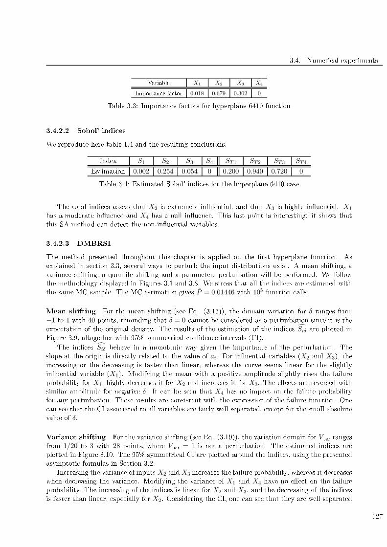
3.4. Numeri al experiments
Variable X1 X2 X3 X4
Importan e fa tor 0.018 0.679 0.302 0
Table 3.3: Importan e fa tors for hyperplane 6410 fun tion
3.4.2.2 Sobol' indi es
We reprodu e here table 1.4 and the resulting on lusions.
Index S1 S2 S3 S4 ST1 ST2 ST3 ST4
Estimation 0.002 0.254 0.054 0 0.200 0.940 0.720 0
Table 3.4: Estimated Sobol' indi es for the hyperplane 6410 ase
The total indi es assess that X2 is extremely inuential, and that X3 is highly inuential. X1
has a moderate inuen e and X4 has a null inuen e. This last point is interesting: it shows that
this SA method an dete t the non-inuential variables.
3.4.2.3 DMBRSI
The method presented throughout this hapter is applied on the rst hyperplane fun tion. As
explained in se tion 3.3, several ways to perturb the input distributions exist. A mean shifting, a
varian e shifting, a quantile shifting and a parameters perturbation will be performed. We follow
the methodology displayed in Figures 3.1 and 3.8. We stress that all the indi es are estimated with
the same MC sample. The MC estimation gives P = 0.01446 with 105 fun tion alls.
Mean shifting For the mean shifting (see Eq. (3.15)), the domain variation for δ ranges from
−1 to 1 with 40 points, reminding that δ = 0 annot be onsidered as a perturbation sin e it is the
expe tation of the original density. The results of the estimation of the indi es Siδ are plotted in
Figure 3.9, altogether with 95% symmetri al onden e intervals (CI).
The indi es Siδ behave in a monotoni way given the importan e of the perturbation. The
slope at the origin is dire tly related to the value of ai. For inuential variables (X2 and X3), the
in reasing or the de reasing is faster than linear, whereas the urve seems linear for the slightly
inuential variable (X1). Modifying the mean with a positive amplitude slightly rises the failure
probability for X1, highly de reases it for X2 and in reases it for X3. The ee ts are reversed with
similar amplitude for negative δ. It an be seen that X4 has no impa t on the failure probability
for any perturbation. Those results are onsistent with the expression of the failure fun tion. One
an see that the CI asso iated to all variables are fairly well separated, ex ept for the small absolute
value of δ.
Varian e shifting For the varian e shifting (see Eq. (3.19)), the variation domain for Vper
ranges
from 1/20 to 3 with 28 points, where Vper
= 1 is not a perturbation. The estimated indi es are
plotted in Figure 3.10. The 95% symmetri al CI are plotted around the indi es, using the presented
asymptoti formulas in Se tion 3.2.
In reasing the varian e of inputs X2 and X3 in reases the failure probability, whereas it de reases
when de reasing the varian e. Modifying the varian e of X1 and X4 have no ee t on the failure
probability. The in reasing of the indi es is linear for X2 and X3, and the de reasing of the indi es
is faster than linear, espe ially for X2. Considering the CI, one an see that they are well separated
127

3. Density Modifi ation Based Reliability Sensitivity Indi es
Figure 3.9: Estimated indi es Siδ for the 6410 hyperplane fun tion with a mean shifting
Figure 3.10: Estimated indi es Si,Vffor hyperplane fun tion with a varian e shifting
for variables X2 and X3, assessing the relative importan e of these variables. On the other hand,
the CI asso iated to X1 and X4 are not separated and ontain 0. Inuen e of X1 and X4 annot
thus be separated - but is estimated as null for both variables.
Quantile shifting
We rst perturb the 5th per entile. The tail is perturbed in su h ways that it weights between 1%
128

3.4. Numeri al experiments
and 10%. The results are displayed in Figure 3.11.
Figure 3.11: 5th per entile perturbation on the hyperplane 6410 test ase
Con erning the left-hand tail, this gure shows the dominant role of variable X2. Ee ts of
variables X1 and X3 are small whereas the indi es asso iated to X4 are null, assessing the non-
inuen e of the last variable - at least when perturbing the left-hand tail.
The rst quartile or 25th per entile is then perturbed. The weight of the tail under the 25th
per entile (meaning the left-hand tail) of the input varies between 10% and 40%. The result of the
numeri al experiments are displayed in Figure 3.12.
This plot shows that an in rease of the 1st quartile leads to an in rease of the failure probability
for variable X2 whereas it leads to a de rease for variables X3 and X1 in order of inuen e. A
quantile perturbation on variable X4 has no ee t on the failure probability. On the other hand,
when de reasing the weight of the 1st quartile, the failure probability in reases for variable X3 and
X1, and de reases for variable X2.
We then perturb the se ond quartile or median. The density is perturbed so that the left-hand
tail weight varies between 25% and 75%. The results are displayed in Figure 3.13.
This last graph shows the relative importan e of X3 and X2. X1 behaves as X3, only with a
smaller ee t. This is relevant given the expression of the model.
Let us now perturb the third quartile or 75th per entile. The weight of the pdf under the 75th
per entile of the standard Gaussian varies between 60% and 90% - whi h is the same as perturbing
the weight of the right-hand tail between 10% and 40%. The result of the numeri al experiments
are displayed in Figure 3.14.
This shows that the most inuential variable when perturbing the 3rd quartile is variable X3, then
omes variable X2, then variable X1. Perturbing variable X4 has no ee t on the failure probability,
as expe ted. We pro eed as before and perturb a more extreme quantile, namely the 95th per entile.It varies between 90% and 99%. The results are displayed in Figure 3.15.
129
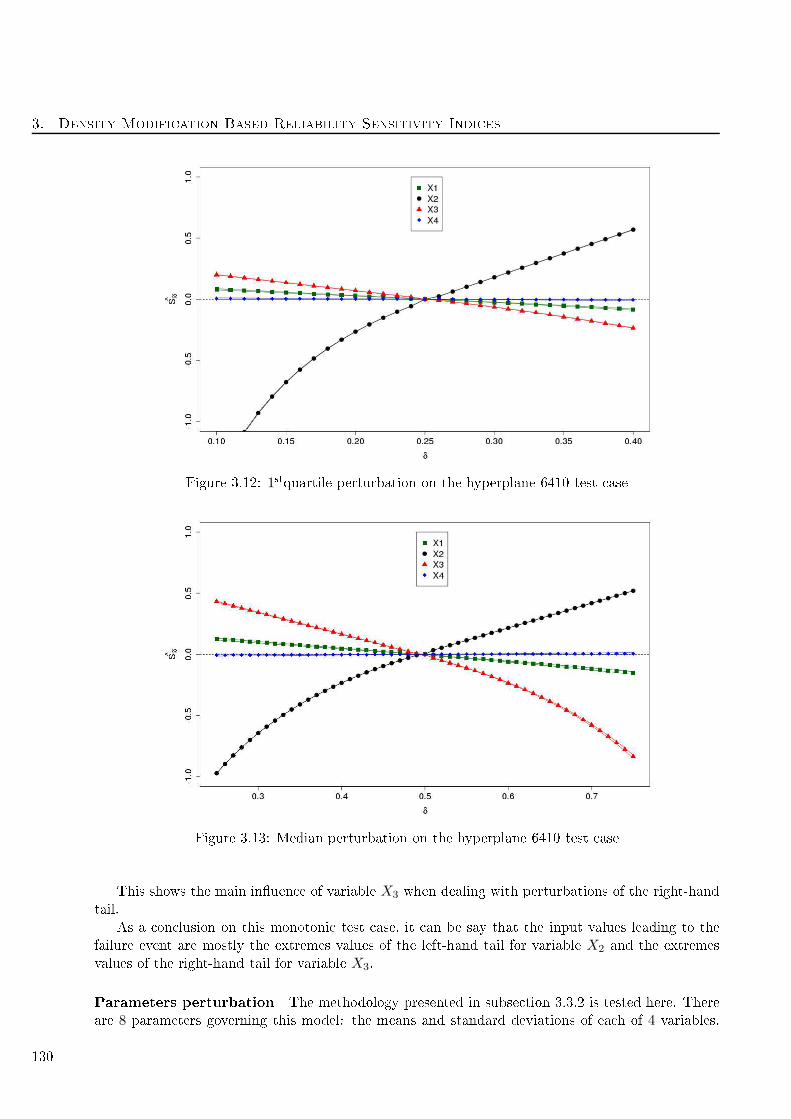
3. Density Modifi ation Based Reliability Sensitivity Indi es
Figure 3.12: 1stquartile perturbation on the hyperplane 6410 test ase
Figure 3.13: Median perturbation on the hyperplane 6410 test ase
This shows the main inuen e of variable X3 when dealing with perturbations of the right-hand
tail.
As a on lusion on this monotoni test ase, it an be say that the input values leading to the
failure event are mostly the extremes values of the left-hand tail for variable X2 and the extremes
values of the right-hand tail for variable X3.
Parameters perturbation The methodology presented in subse tion 3.3.2 is tested here. There
are 8 parameters governing this model: the means and standard deviations of ea h of 4 variables.
130
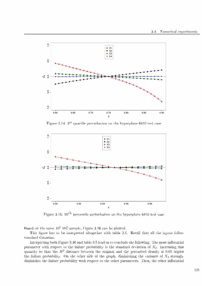
3.4. Numeri al experiments
Figure 3.14: 3rd quartile perturbation on the hyperplane 6410 test ase
Figure 3.15: 95th per entile perturbation on the hyperplane 6410 test ase
Based on the same 105 MC sample, Figure 3.16 an be plotted.
This gure has to be interpreted altogether with table 3.5. Re all that all the inputs follow
standard Gaussian.
Interpreting both Figure 3.16 and table 3.5 lead us to on lude the following. The most inuential
parameter with respe t to the failure probability is the standard deviation of X2. In reasing this
quantity so that the H2distan e between the original and the perturbed density is 0.05 triples
the failure probability. On the other side of the graph, diminishing the varian e of X2 strongly
diminishes the failure probability with respe t to the other parameters. Then, the other inuential
131
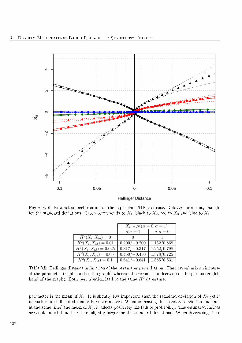
3. Density Modifi ation Based Reliability Sensitivity Indi es
−6
−4
−2
02
4
Hellinger Distance
Siδ^
0.1 0.05 0 0.05 0.1
Figure 3.16: Parameters perturbation on the hyperplane 6410 test ase. Dots are for means, triangle
for the standard deviations. Green orresponds to X1, bla k to X2, red to X3 and blue to X4.
Xi ∼ N (µ = 0, σ = 1)µ|σ = 1 σ|µ = 0
H2(Xi,Xiδ) = 0 0 1
H2(Xi,Xiδ) = 0.01 0.200/−0.200 1.152/0.868
H2(Xi,Xiδ) = 0.025 0.317/−0.317 1.252/0.798
H2(Xi,Xiδ) = 0.05 0.450/−0.450 1.378/0.725
H2(Xi,Xiδ) = 0.1 0.641/−0.641 1.585/0.631
Table 3.5: Hellinger distan e in fun tion of the parameter perturbation. The rst value is an in rease
of the parameter (right hand of the graph) whereas the se ond is a de rease of the parameter (left
hand of the graph). Both perturbation lead to the same H2departure.
parameter is the mean of X2. It is slightly less important than the standard deviation of X2 yet it
is mu h more inuential than others parameters. When in reasing the standard deviation and (not
at the same time) the mean of X3, it ae ts positively the failure probability. The estimated indi es
are onfounded, but the CI are slightly larger for the standard deviations. When de reasing these
132
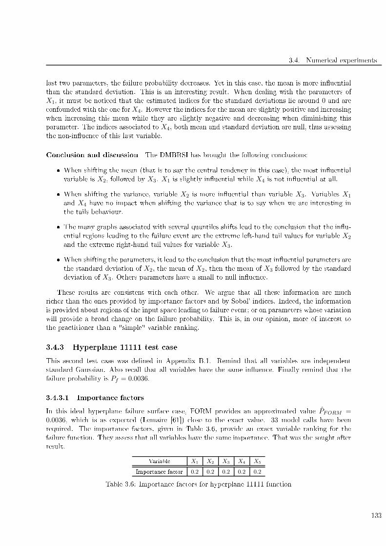
3.4. Numeri al experiments
last two parameters, the failure probability de reases. Yet in this ase, the mean is more inuential
than the standard deviation. This is an interesting result. When dealing with the parameters of
X1, it must be noti ed that the estimated indi es for the standard deviations lie around 0 and are
onfounded with the one forX4. However the indi es for the mean are slightly positive and in reasing
when in reasing this mean while they are slightly negative and de reasing when diminishing this
parameter. The indi es asso iated to X4, both mean and standard deviation are null, thus assessing
the non-inuen e of this last variable.
Con lusion and dis ussion The DMBRSI has brought the following on lusions:
When shifting the mean (that is to say the entral tenden y in this ase), the most inuential
variable is X2, followed by X3. X1 is slightly inuential while X4 is not inuential at all.
When shifting the varian e, variable X2 is more inuential than variable X3. Variables X1
and X4 have no impa t when shifting the varian e that is to say when we are interesting in
the tails behaviour.
The many graphs asso iated with several quantiles shifts lead to the on lusion that the inu-
ential regions leading to the failure event are the extreme left-hand tail values for variable X2
and the extreme right-hand tail values for variable X3.
When shifting the parameters, it lead to the on lusion that the most inuential parameters are
the standard deviation of X2, the mean of X2, then the mean of X3 followed by the standard
deviation of X3. Others parameters have a small to null inuen e.
These results are onsistent with ea h other. We argue that all these information are mu h
ri her than the ones provided by importan e fa tors and by Sobol' indi es. Indeed, the information
is provided about regions of the input spa e leading to failure event; or on parameters whose variation
will provide a broad hange on the failure probability. This is, in our opinion, more of interest to
the pra titioner than a "simple" variable ranking.
3.4.3 Hyperplane 11111 test ase
This se ond test ase was dened in Appendix B.1. Remind that all variables are independent
standard Gaussian. Also re all that all variables have the same inuen e. Finally remind that the
failure probability is Pf = 0.0036.
3.4.3.1 Importan e fa tors
In this ideal hyperplane failure surfa e ase, FORM provides an approximated value PFORM =0.0036, whi h is as expe ted (Lemaire [61) lose to the exa t value. 33 model alls have been
required. The importan e fa tors, given in Table 3.6, provide an exa t variable ranking for the
failure fun tion. They assess that all variables have the same importan e. That was the sought after
result.
Variable X1 X2 X3 X4 X5
Importan e fa tor 0.2 0.2 0.2 0.2 0.2
Table 3.6: Importan e fa tors for hyperplane 11111 fun tion
133
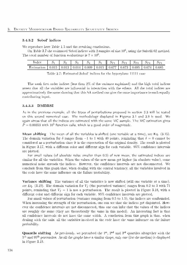
3. Density Modifi ation Based Reliability Sensitivity Indi es
3.4.3.2 Sobol' indi es
We reprodu e here Table 1.5 and the resulting on lusions.
On Table 3.7 the estimated Sobol indi es with 2 samples of size 106, using the Saltelli 02 method.
The total number of fun tion evaluations is 7× 10⁶.
Index S1 S2 S3 S4 S5 ST1 ST2 ST3 ST4 ST5
Estimation 0.015 0.013 0.014 0.009 0.015 0.677 0.673 0.695 0.674 0.685
Table 3.7: Estimated Sobol' indi es for the hyperplane 11111 ase
The weak rst order indi es (less than 2% of the varian e explained) and the high total indi es
assess that all the variables are inuential in intera tion with the others. All the total indi es are
approximatively the same showing that this SA method an give the same importan e to ea h equally
ontributing input.
3.4.3.3 DMBRSI
As in the previous example, all the types of perturbations proposed in se tion 3.3 will be tested
on this se ond numeri al ase. The methodology displayed in Figures 3.1 and 3.8 is used. We
again stress that all the indi es are estimated with the same MC sample. The MC estimation gives
P = 0.00353 with 105 fun tion alls, whi h is a good order of magnitude.
Mean shifting The mean of all the variables is shifted (one variable at a time), see Eq. (3.15).
The domain variation for δ ranges from −1 to 1 with 40 points, reminding that δ = 0 annot be
onsidered as a perturbation sin e it is the expe tation of the original density. The result is plotted
in Figure 3.17, with a dierent olor and dierent sign for ea h variable. 95% onden e intervals
are plotted.
For small values (of absolute value smaller than 0.5) of new mean, the estimated indi es are
similar for all the variables. When the values of the new mean get higher (in absolute value), some
numeri al noise spreads the indi es. However, the onden e intervals are not dis onne ted. We
on lude from this graph that, when dealing with the entral tenden y, all the variables involved in
the ode have the same inuen e on the failure probability.
Varian e shifting The varian e of all the variables is now shifted (still one variable at a time),
see Eq. (3.19). The domain variation for Vf (the perturbed varian e) ranges from 0.2 to 3 with 71points, reminding that Vf = 1 is not a perturbation. The result is plotted in Figure 3.18, with a
dierent olor and dierent sign for ea h variable. 95% onden e intervals are plotted.
For small values of perturbation (varian e ranging from 0.5 to 1.5), the indi es are onfounded.When in reasing the strength of the perturbation, one an see that the indi es get disjointed. How-
ever the onden e intervals are not dis onne ted, thus one an infer that the values of the indi es
are roughly the same (they are theoreti ally the same in this model). An interesting fa t is that
all onden e intervals do not have the same width. A on lusion from this graph is that, when
dealing with the tails, all the variables involved in the ode have the same inuen e on the failure
probability.
Quantile shifting As previously, we perturbed the 1st, 2nd and 3rd quartiles altogether with the
5th and 95th per entiles. As all the graphs have a similar shape, only one (for the median) is displayed
in Figure 3.19.
134
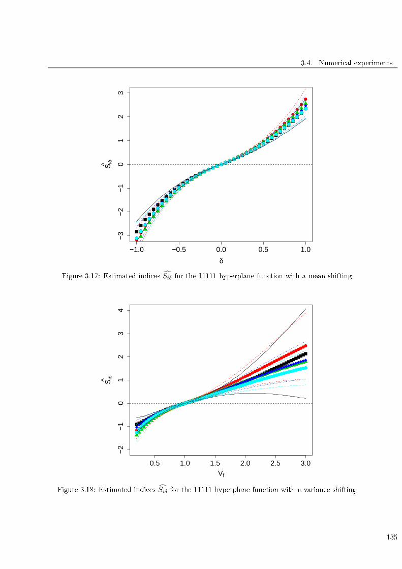
3.4. Numeri al experiments
−1.0 −0.5 0.0 0.5 1.0
−3
−2
−1
01
23
δ
Siδ^
Figure 3.17: Estimated indi es Siδ for the 11111 hyperplane fun tion with a mean shifting
0.5 1.0 1.5 2.0 2.5 3.0
−2
−1
01
23
4
Vf
Siδ^
Figure 3.18: Estimated indi es Siδ for the 11111 hyperplane fun tion with a varian e shifting
135
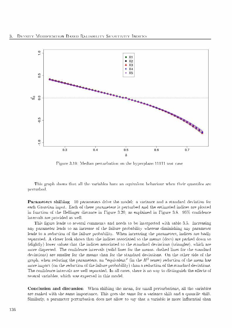
3. Density Modifi ation Based Reliability Sensitivity Indi es
Figure 3.19: Median perturbation on the hyperplane 11111 test ase
This graph shows that all the variables have an equivalent behaviour when their quantiles are
perturbed.
Parameters shifting 10 parameters drive the model: a varian e and a standard deviation for
ea h Gaussian input. Ea h of these parameters is perturbed and the estimated indi es are plotted
in fun tion of the Hellinger distan e in Figure 3.20, as explained in Figure 3.8. 95% onden e
intervals are provided as well.
This gure leads to several omments and needs to be interpreted with table 3.5. In reasing
any parameter leads to an in rease of the failure probability whereas diminishing any parameter
leads to a redu tion of the failure probability. When in reasing the parameters, indi es are badly
separated. A loser look shows that the indi es asso iated to the means (dots) are pa ked down to
(slightly) lower values that the indi es asso iated to the standard deviations (triangles), whi h are
more dispersed. The onden e intervals (solid lines for the means, dashed lines for the standard
deviations) are smaller for the means than for the standard deviations. On the other side of the
graph, when redu ing the parameters, an "equivalent" (in the H2sense) redu tion of the mean has
more impa t (on the redu tion of the failure probability) than a redu tion of the standard deviations.
The onden e intervals are well separated. In all ases, there is no way to distinguish the ee ts of
several variables, whi h was expe ted in this model.
Con lusion and dis ussion When shifting the mean, for small perturbations, all the variables
are ranked with the same importan e. This goes the same for a varian e shift and a quantile shift.
Similarly, a parameter perturbation does not allow to say that a variable is more inuential than
136
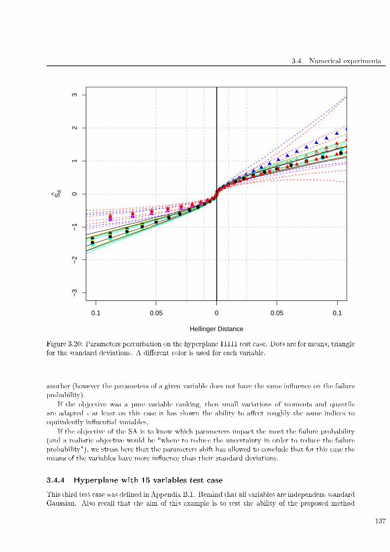
3.4. Numeri al experiments
−3
−2
−1
01
23
Hellinger Distance
Siδ^
0.1 0.05 0 0.05 0.1
Figure 3.20: Parameters perturbation on the hyperplane 11111 test ase. Dots are for means, triangle
for the standard deviations. A dierent olor is used for ea h variable.
another (however the parameters of a given variable does not have the same inuen e on the failure
probability).
If the obje tive was a pure variable ranking, then small variations of moments and quantile
are adapted - at least on this ase it has shown the ability to ae t roughly the same indi es to
equivalently inuential variables.
If the obje tive of the SA is to know whi h parameters impa t the most the failure probability
(and a realisti obje tive would be "where to redu e the un ertainty in order to redu e the failure
probability"), we stress here that the parameters shift has allowed to on lude that for this ase the
means of the variables have more inuen e than their standard deviations.
3.4.4 Hyperplane with 15 variables test ase
This third test ase was dened in Appendix B.1. Remind that all variables are independent standard
Gaussian. Also re all that the aim of this example is to test the ability of the proposed method
137
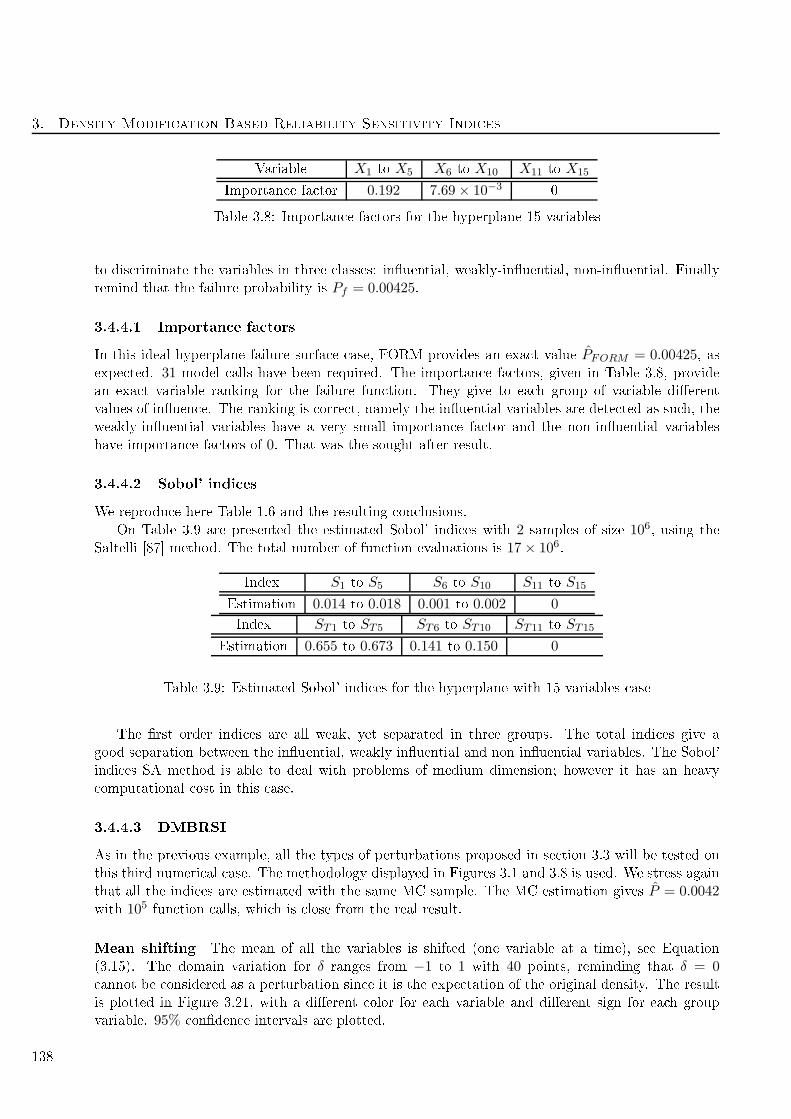
3. Density Modifi ation Based Reliability Sensitivity Indi es
Variable X1 to X5 X6 to X10 X11 to X15
Importan e fa tor 0.192 7.69× 10⁻³⁰
Table 3.8: Importan e fa tors for the hyperplane 15 variables
to dis riminate the variables in three lasses: inuential, weakly-inuential, non-inuential. Finally
remind that the failure probability is Pf = 0.00425.
3.4.4.1 Importan e fa tors
In this ideal hyperplane failure surfa e ase, FORM provides an exa t value PFORM = 0.00425, asexpe ted. 31 model alls have been required. The importan e fa tors, given in Table 3.8, provide
an exa t variable ranking for the failure fun tion. They give to ea h group of variable dierent
values of inuen e. The ranking is orre t, namely the inuential variables are dete ted as su h, the
weakly-inuential variables have a very small importan e fa tor and the non-inuential variables
have importan e fa tors of 0. That was the sought after result.
3.4.4.2 Sobol' indi es
We reprodu e here Table 1.6 and the resulting on lusions.
On Table 3.9 are presented the estimated Sobol' indi es with 2 samples of size 106, using the
Saltelli [87 method. The total number of fun tion evaluations is 17× 106.
Index S1 to S5 S6 to S10 S11 to S15
Estimation 0.014 to 0.018 0.001 to 0.002 0
Index ST1 to ST5 ST6 to ST10 ST11 to ST15
Estimation 0.655 to 0.673 0.141 to 0.150 0
Table 3.9: Estimated Sobol' indi es for the hyperplane with 15 variables ase
The rst order indi es are all weak, yet separated in three groups. The total indi es give a
good separation between the inuential, weakly inuential and non inuential variables. The Sobol'
indi es SA method is able to deal with problems of medium dimension; however it has an heavy
omputational ost in this ase.
3.4.4.3 DMBRSI
As in the previous example, all the types of perturbations proposed in se tion 3.3 will be tested on
this third numeri al ase. The methodology displayed in Figures 3.1 and 3.8 is used. We stress again
that all the indi es are estimated with the same MC sample. The MC estimation gives P = 0.0042with 105 fun tion alls, whi h is lose from the real result.
Mean shifting The mean of all the variables is shifted (one variable at a time), see Equation
(3.15). The domain variation for δ ranges from −1 to 1 with 40 points, reminding that δ = 0 annot be onsidered as a perturbation sin e it is the expe tation of the original density. The result
is plotted in Figure 3.21, with a dierent olor for ea h variable and dierent sign for ea h group
variable. 95% onden e intervals are plotted.
138

3.4. Numeri al experiments
−1.0 −0.5 0.0 0.5 1.0
−3
−2
−1
01
23
δ
Siδ^
Figure 3.21: Estimated indi es Siδ for the 15 variables hyperplane fun tion with a mean shifting
For the inuential variables (big dots), in reasing the mean in reases the failure probability
whereas de reasing this parameter de reases the failure probability. However distinguish the ee ts
of the weakly-inuential variables (triangles) from the ee ts of the non-inuential variables (small
dots) is not possible due to the overing of the onden e intervals. So far, DMBRSI does not allow
to separate the ee ts of the two last groups of variables. However, another test with a MC size of
106 draws (graphs non provided here) allows a good separation of the weakly and non-inuential
variables.
Varian e shifting The varian e of all the variables is now shifted (still one variable at a time),
see Equation (3.19). The domain variation for Vf (the perturbed varian e) ranges from 0.2 to 3 with71 points, reminding that Vf = 1 is not a perturbation. The result is plotted in Figure 3.22, with a
dierent olor and dierent sign for ea h variable. 95% symmetri al onden e intervals are plotted.
The inuential variables (big dots) are well separated from the others. As expe ted for these
variables, in reasing (respe tively de reasing) the varian e in reases (respe tively de reases) the
failure probability. However, the ee ts for the weakly-inuential (triangles) and non-inuential
(small dots) variables, the ee ts are hardly separable (see the onden e intervals). As well as
previously, DMBRSI does not allow to separate the ee ts of the two last groups of variables (weakly
and non-inuential).
However, in reasing the sample size of a fa tor 10 (graph not provided here) still does not allow to
separate the ee ts of the last two groups of variable. This might be due to the relative null-inuen e
of a varian e shift in the last 10 variables.
139
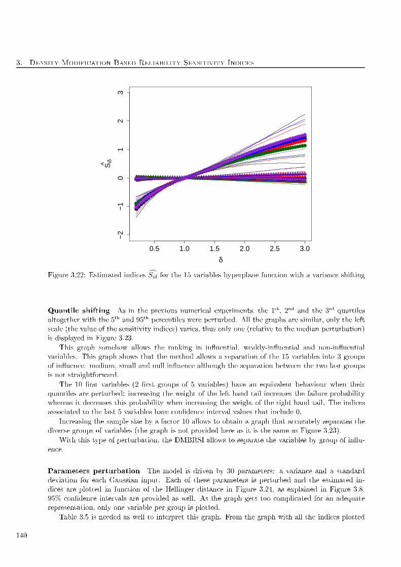
3. Density Modifi ation Based Reliability Sensitivity Indi es
0.5 1.0 1.5 2.0 2.5 3.0
−2
−1
01
23
δ
Siδ^
Figure 3.22: Estimated indi es Siδ for the 15 variables hyperplane fun tion with a varian e shifting
Quantile shifting As in the previous numeri al experiments, the 1st, 2nd and the 3rd quartiles
altogether with the 5th and 95th per entiles were perturbed. All the graphs are similar, only the left
s ale (the value of the sensitivity indi es) varies, thus only one (relative to the median perturbation)
is displayed in Figure 3.23.
This graph somehow allows the ranking in inuential, weakly-inuential and non-inuential
variables. This graph shows that the method allows a separation of the 15 variables into 3 groups
of inuen e: medium, small and null inuen e although the separation between the two last groups
is not straightforward.
The 10 rst variables (2 rst groups of 5 variables) have an equivalent behaviour when their
quantiles are perturbed: in reasing the weight of the left-hand tail in reases the failure probability
whereas it de reases this probability when in reasing the weight of the right-hand tail. The indi es
asso iated to the last 5 variables have onden e interval values that in lude 0.
In reasing the sample size by a fa tor 10 allows to obtain a graph that a urately separates the
diverse groups of variables (the graph is not provided here as it is the same as Figure 3.23).
With this type of perturbation, the DMBRSI allows to separate the variables by group of inu-
en e.
Parameters perturbation The model is driven by 30 parameters: a varian e and a standard
deviation for ea h Gaussian input. Ea h of these parameters is perturbed and the estimated in-
di es are plotted in fun tion of the Hellinger distan e in Figure 3.24, as explained in Figure 3.8.
95% onden e intervals are provided as well. As the graph gets too ompli ated for an adequate
representation, only one variable per group is plotted.
Table 3.5 is needed as well to interpret this graph. From the graph with all the indi es plotted
140
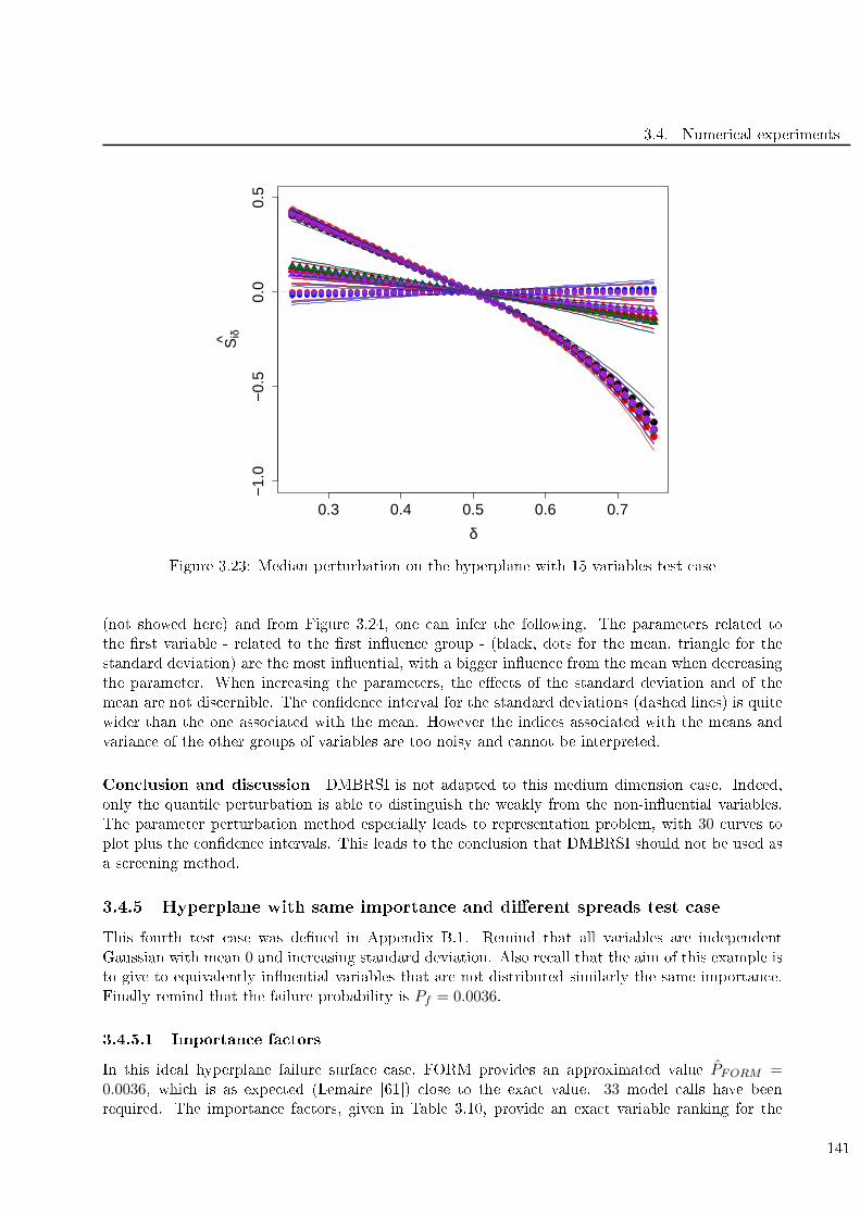
3.4. Numeri al experiments
0.3 0.4 0.5 0.6 0.7
−1.
0−
0.5
0.0
0.5
δ
Siδ^
Figure 3.23: Median perturbation on the hyperplane with 15 variables test ase
(not showed here) and from Figure 3.24, one an infer the following. The parameters related to
the rst variable - related to the rst inuen e group - (bla k, dots for the mean, triangle for the
standard deviation) are the most inuential, with a bigger inuen e from the mean when de reasing
the parameter. When in reasing the parameters, the ee ts of the standard deviation and of the
mean are not dis ernible. The onden e interval for the standard deviations (dashed lines) is quite
wider than the one asso iated with the mean. However the indi es asso iated with the means and
varian e of the other groups of variables are too noisy and annot be interpreted.
Con lusion and dis ussion DMBRSI is not adapted to this medium dimension ase. Indeed,
only the quantile perturbation is able to distinguish the weakly from the non-inuential variables.
The parameter perturbation method espe ially leads to representation problem, with 30 urves to
plot plus the onden e intervals. This leads to the on lusion that DMBRSI should not be used as
a s reening method.
3.4.5 Hyperplane with same importan e and dierent spreads test ase
This fourth test ase was dened in Appendix B.1. Remind that all variables are independent
Gaussian with mean 0 and in reasing standard deviation. Also re all that the aim of this example is
to give to equivalently inuential variables that are not distributed similarly the same importan e.
Finally remind that the failure probability is Pf = 0.0036.
3.4.5.1 Importan e fa tors
In this ideal hyperplane failure surfa e ase, FORM provides an approximated value PFORM =0.0036, whi h is as expe ted (Lemaire [61) lose to the exa t value. 33 model alls have been
required. The importan e fa tors, given in Table 3.10, provide an exa t variable ranking for the
141
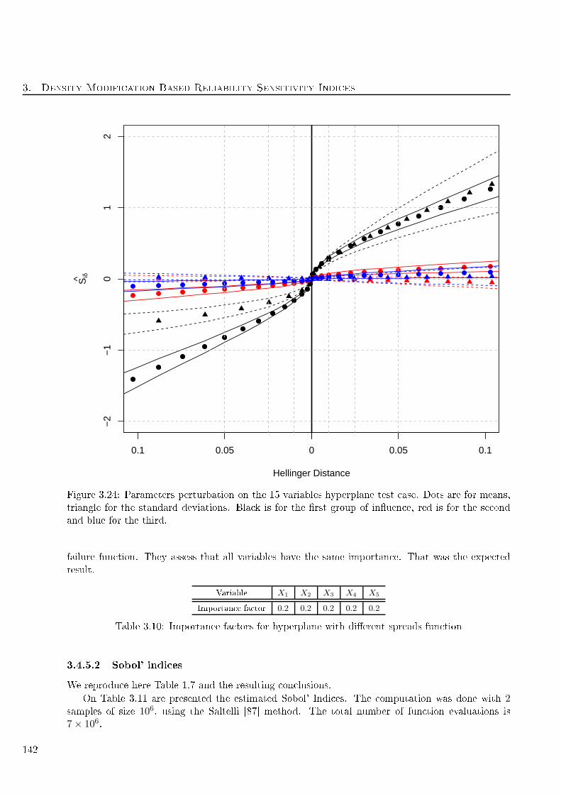
3. Density Modifi ation Based Reliability Sensitivity Indi es
−2
−1
01
2
Hellinger Distance
Siδ^
0.1 0.05 0 0.05 0.1
Figure 3.24: Parameters perturbation on the 15 variables hyperplane test ase. Dots are for means,
triangle for the standard deviations. Bla k is for the rst group of inuen e, red is for the se ond
and blue for the third.
failure fun tion. They assess that all variables have the same importan e. That was the expe ted
result.
Variable X1 X2 X3 X4 X5
Importan e fa tor 0.2 0.2 0.2 0.2 0.2
Table 3.10: Importan e fa tors for hyperplane with dierent spreads fun tion
3.4.5.2 Sobol' indi es
We reprodu e here Table 1.7 and the resulting on lusions.
On Table 3.11 are presented the estimated Sobol' Indi es. The omputation was done with 2samples of size 106, using the Saltelli [87 method. The total number of fun tion evaluations is
7× 10⁶.
142

3.4. Numeri al experiments
Index S1 S2 S3 S4 S5 ST1 ST2 ST3 ST4 ST5
Estimation 0.027 0.028 0.025 0.025 0.028 0.611 0.622 0.618 0.618 0.624
Table 3.11: Estimated Sobol' indi es for the hyperplane with dierent spreads ase
The weak rst order indi es (less than 3% of the varian e explained) and the high total indi es
assess that all variables are inuential in intera tion with the others, and that no variable is inuential
on its own. All the total indi es are approximatively equal showing that this SA method gives to
ea h equally ontributing variable the same importan e, despite their dierent spread.
3.4.5.3 DMBRSI
One an noti e that the dierent inputs follow various distributions (unlike the other examples), thus
the question of "equivalent" perturbation arises. Due to this non-similarity of the distributions, only
a (modied) mean shift, a quantile shift and a parameter shift will be applied on this test ase. It
has been dis ussed further in Se tion 3.3.1.3.
Mean shifting As stressed in Se tion 3.3.1.3 the hoi e has been made to shift the mean relatively
to the standard deviation, hen e in luding the spread of the various inputs in their respe tive
perturbation. So for any input, the original distribution is perturbed so that its mean is the original
one plus δ times its standard deviation, δ ranging from −1 to 1 with 40 points. The results of the
numeri al experiment are displayed in Figure 3.25.
−1.0 −0.5 0.0 0.5 1.0
−3
−2
−1
01
23
δ
Siδ^
Figure 3.25: Estimated indi es Siδ for the hyperplane with dierent spreads ase with a mean shifting
143
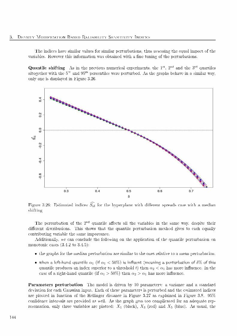
3. Density Modifi ation Based Reliability Sensitivity Indi es
The indi es have similar values for similar perturbations, thus assessing the equal impa t of the
variables. However this information was obtained with a ne tuning of the perturbations.
Quantile shifting As in the previous numeri al experiments, the 1st, 2nd and the 3rd quartiles
altogether with the 5th and 95th per entiles were perturbed. As the graphs behave in a similar way,
only one is displayed in Figure 3.26.
Figure 3.26: Estimated indi es Siδ for the hyperplane with dierent spreads ase with a median
shifting
The perturbation of the 2nd quantile ae ts all the variables in the same way, despite their
dierent distributions. This shows that the quantile perturbation method gives to ea h equally
ontributing variable the same importan e.
Additionally, we an on lude the following on the appli ation of the quantile perturbation on
monotoni ases (3.4.2 to 3.4.5):
the graphs for the median perturbation are similar to the ones relative to a mean perturbation.
when a left-hand quantile α1 (if α1 < 50%) is inuent (meaning a perturbation of δ% of this
quantile produ es an index superior to a threshold t) then α2 < α1 has more inuen e. In the
ase of a right-hand quantile (if α1 > 50%) then α2 > α1 has more inuen e.
Parameters perturbation The model is driven by 10 parameters: a varian e and a standard
deviation for ea h Gaussian input. Ea h of these parameters is perturbed and the estimated indi es
are plotted in fun tion of the Hellinger distan e in Figure 3.27 as explained in Figure 3.8. 95% onden e intervals are provided as well. As the graph gets too ompli ated for an adequate rep-
resentation, only three variables are plotted: X1 (bla k), X3 (red) and X5 (blue). As usual, the
144
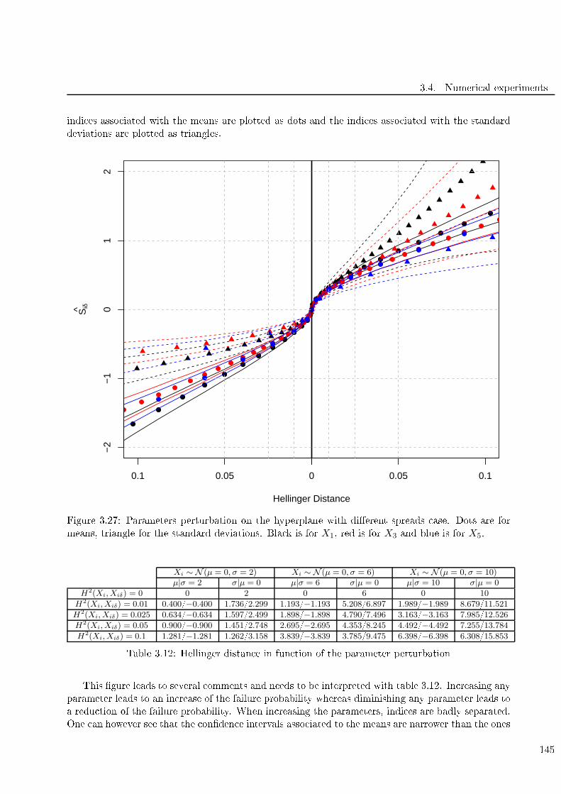
3.4. Numeri al experiments
indi es asso iated with the means are plotted as dots and the indi es asso iated with the standard
deviations are plotted as triangles.
−2
−1
01
2
Hellinger Distance
Siδ^
0.1 0.05 0 0.05 0.1
Figure 3.27: Parameters perturbation on the hyperplane with dierent spreads ase. Dots are for
means, triangle for the standard deviations. Bla k is for X1, red is for X3 and blue is for X5.
Xi ∼ N (µ = 0, σ = 2) Xi ∼ N (µ = 0, σ = 6) Xi ∼ N (µ = 0, σ = 10)µ|σ = 2 σ|µ = 0 µ|σ = 6 σ|µ = 0 µ|σ = 10 σ|µ = 0
H2(Xi, Xiδ) = 0 0 2 0 6 0 10
H2(Xi, Xiδ) = 0.01 0.400/−0.400 1.736/2.299 1.193/−1.193 5.208/6.897 1.989/−1.989 8.679/11.521
H2(Xi, Xiδ) = 0.025 0.634/−0.634 1.597/2.499 1.898/−1.898 4.790/7.496 3.163/−3.163 7.985/12.526
H2(Xi, Xiδ) = 0.05 0.900/−0.900 1.451/2.748 2.695/−2.695 4.353/8.245 4.492/−4.492 7.255/13.784
H2(Xi, Xiδ) = 0.1 1.281/−1.281 1.262/3.158 3.839/−3.839 3.785/9.475 6.398/−6.398 6.308/15.853
Table 3.12: Hellinger distan e in fun tion of the parameter perturbation
This gure leads to several omments and needs to be interpreted with table 3.12. In reasing any
parameter leads to an in rease of the failure probability whereas diminishing any parameter leads to
a redu tion of the failure probability. When in reasing the parameters, indi es are badly separated.
One an however see that the onden e intervals asso iated to the means are narrower than the ones
145
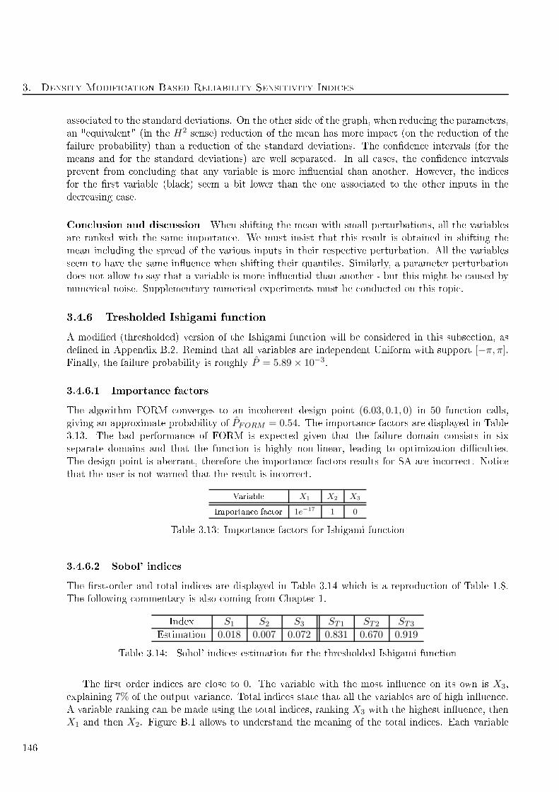
3. Density Modifi ation Based Reliability Sensitivity Indi es
asso iated to the standard deviations. On the other side of the graph, when redu ing the parameters,
an "equivalent" (in the H2sense) redu tion of the mean has more impa t (on the redu tion of the
failure probability) than a redu tion of the standard deviations. The onden e intervals (for the
means and for the standard deviations) are well separated. In all ases, the onden e intervals
prevent from on luding that any variable is more inuential than another. However, the indi es
for the rst variable (bla k) seem a bit lower than the one asso iated to the other inputs in the
de reasing ase.
Con lusion and dis ussion When shifting the mean with small perturbations, all the variables
are ranked with the same importan e. We must insist that this result is obtained in shifting the
mean in luding the spread of the various inputs in their respe tive perturbation. All the variables
seem to have the same inuen e when shifting their quantiles. Similarly, a parameter perturbation
does not allow to say that a variable is more inuential than another - but this might be aused by
numeri al noise. Supplementary numeri al experiments must be ondu ted on this topi .
3.4.6 Tresholded Ishigami fun tion
A modied (thresholded) version of the Ishigami fun tion will be onsidered in this subse tion, as
dened in Appendix B.2. Remind that all variables are independent Uniform with support [−π, π].Finally, the failure probability is roughly P = 5.89 × 10⁻³
.
3.4.6.1 Importan e fa tors
The algorithm FORM onverges to an in oherent design point (6.03, 0.1, 0) in 50 fun tion alls,
giving an approximate probability of PFORM = 0.54. The importan e fa tors are displayed in Table
3.13. The bad performan e of FORM is expe ted given that the failure domain onsists in six
separate domains and that the fun tion is highly non-linear, leading to optimization di ulties.
The design point is aberrant, therefore the importan e fa tors results for SA are in orre t. Noti e
that the user is not warned that the result is in orre t.
Variable X1 X2 X3
Importan e fa tor 1e−17 1 0
Table 3.13: Importan e fa tors for Ishigami fun tion
3.4.6.2 Sobol' indi es
The rst-order and total indi es are displayed in Table 3.14 whi h is a reprodu tion of Table 1.8.
The following ommentary is also oming from Chapter 1.
Index S1 S2 S3 ST1 ST2 ST3
Estimation 0.018 0.007 0.072 0.831 0.670 0.919
Table 3.14: Sobol' indi es estimation for the thresholded Ishigami fun tion
The rst order indi es are lose to 0. The variable with the most inuen e on its own is X3,
explaining 7% of the output varian e. Total indi es state that all the variables are of high inuen e.
A variable ranking an be made using the total indi es, ranking X3 with the highest inuen e, then
X1 and then X2. Figure B.1 allows to understand the meaning of the total indi es. Ea h variable
146
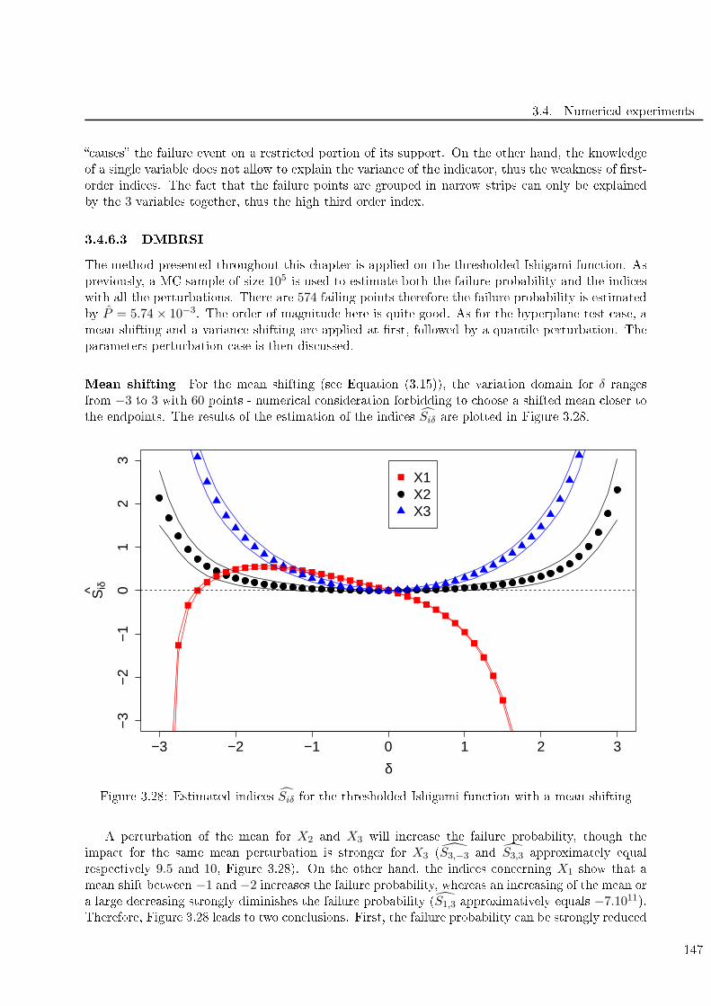
3.4. Numeri al experiments
auses the failure event on a restri ted portion of its support. On the other hand, the knowledge
of a single variable does not allow to explain the varian e of the indi ator, thus the weakness of rst-
order indi es. The fa t that the failure points are grouped in narrow strips an only be explained
by the 3 variables together, thus the high third order index.
3.4.6.3 DMBRSI
The method presented throughout this hapter is applied on the thresholded Ishigami fun tion. As
previously, a MC sample of size 105 is used to estimate both the failure probability and the indi es
with all the perturbations. There are 574 failing points therefore the failure probability is estimated
by P = 5.74 × 10⁻³. The order of magnitude here is quite good. As for the hyperplane test ase, a
mean shifting and a varian e shifting are applied at rst, followed by a quantile perturbation. The
parameters perturbation ase is then dis ussed.
Mean shifting For the mean shifting (see Equation (3.15)), the variation domain for δ ranges
from −3 to 3 with 60 points - numeri al onsideration forbidding to hoose a shifted mean loser to
the endpoints. The results of the estimation of the indi es Siδ are plotted in Figure 3.28.
−3 −2 −1 0 1 2 3
−3
−2
−1
01
23
δ
Siδ^
X1X2X3
Figure 3.28: Estimated indi es Siδ for the thresholded Ishigami fun tion with a mean shifting
A perturbation of the mean for X2 and X3 will in rease the failure probability, though the
impa t for the same mean perturbation is stronger for X3 (S3,−3 and S3,3 approximately equal
respe tively 9.5 and 10, Figure 3.28). On the other hand, the indi es on erning X1 show that a
mean shift between −1 and −2 in reases the failure probability, whereas an in reasing of the mean or
a large de reasing strongly diminishes the failure probability (S1,3 approximatively equals −7.1011).Therefore, Figure 3.28 leads to two on lusions. First, the failure probability an be strongly redu ed
147
3. Density Modifi ation Based Reliability Sensitivity Indi es
when in reasing the mean of the rst variable X1 (this is also provided by Figure B.1 wherein all
failure points have a negative value of X1). Se ond, any hange in the mean for X2 or X3 will lead to
an in rease of the failure probability. The onden e intervals are well separated, ex ept in the −1to 1 zone. One an noti e that the onden e interval asso iated to X2 ontains 0 between values
of δ from −1.5 to 1.5, thus the asso iated indi es might be null in these ase. This has to be taken
into a ount when assessing the relative importan e of X2.
Varian e shifting For varian e shifting, the variation domain for Vper
ranges from 1 to 5 with 40points. Let us re all that the original varian e is Var[Xi] = π2/3 ≃ 3.29. The modied pdf when
shifting the varian e and keeping the same expe tation is proportional to a trun ated Gaussian when
de reasing the varian e. When in reasing the varian e, the perturbed distribution is a symmetri al
distribution with 2 modes lose to the endpoints of the support (see Figure 3.3). The results of the
estimation of the indi es Si,Vper
are plotted in Figure 3.29. The upper gure is a zoom where the
Si,Vper
axis lies into [−0.5, 0.5]. The lower gure shows almost the whole range variation for Si,Vper
.
The urves ross for the value of Vper
that orresponds to the original varian e, namely π2/2.
Figure 3.29 (upper part) shows that a hange in the varian e has little ee t on X2 and X1,
though the hange is of opposite ee t on the failure probability. However, onsidering that the
indi es S2,Vper,i
and S1,Vper,i
lie between −0.4 and 0.4, one an on lude that the varian e of theses
variables are not of great inuen e on the failure probability. On the other hand, Figure 3.29 (lower
part) shows that any redu tion of Var [X3] strongly de reases the failure probability, and that an
in rease of the varian e slightly in reases the failure probability. This is relevant with the expression
of the failure surfa e, as X3 is fourth powered and multiplied by the sinus of X1. A varian e
de reasing as formulated gives a distribution on entrated around 0. De reasing Var [X3] shrinksthe on erned term in G(X). Therefore it redu es the failure probability. The onden e intervals
asso iated to X3 are broadly separated from the others.
Quantile shifting First, the 5th per entile is perturbed and the result is displayed in Figure 3.30.
This graph shows that for variable X1, an in rease of the weight of the right-hand tail diminishes
the failure probability and a de rease of the weight ae ts positively the failure probability. It is the
opposite for variable X2 and X3: an in rease of the weight of the left-hand tail in reases the failure
probability and a de rease of the weight de reases the failure probability. The ee t is stronger for
variable X3.
Then, the rst quartile is perturbed. The results of the experiment are plotted in Figure 3.31.
148
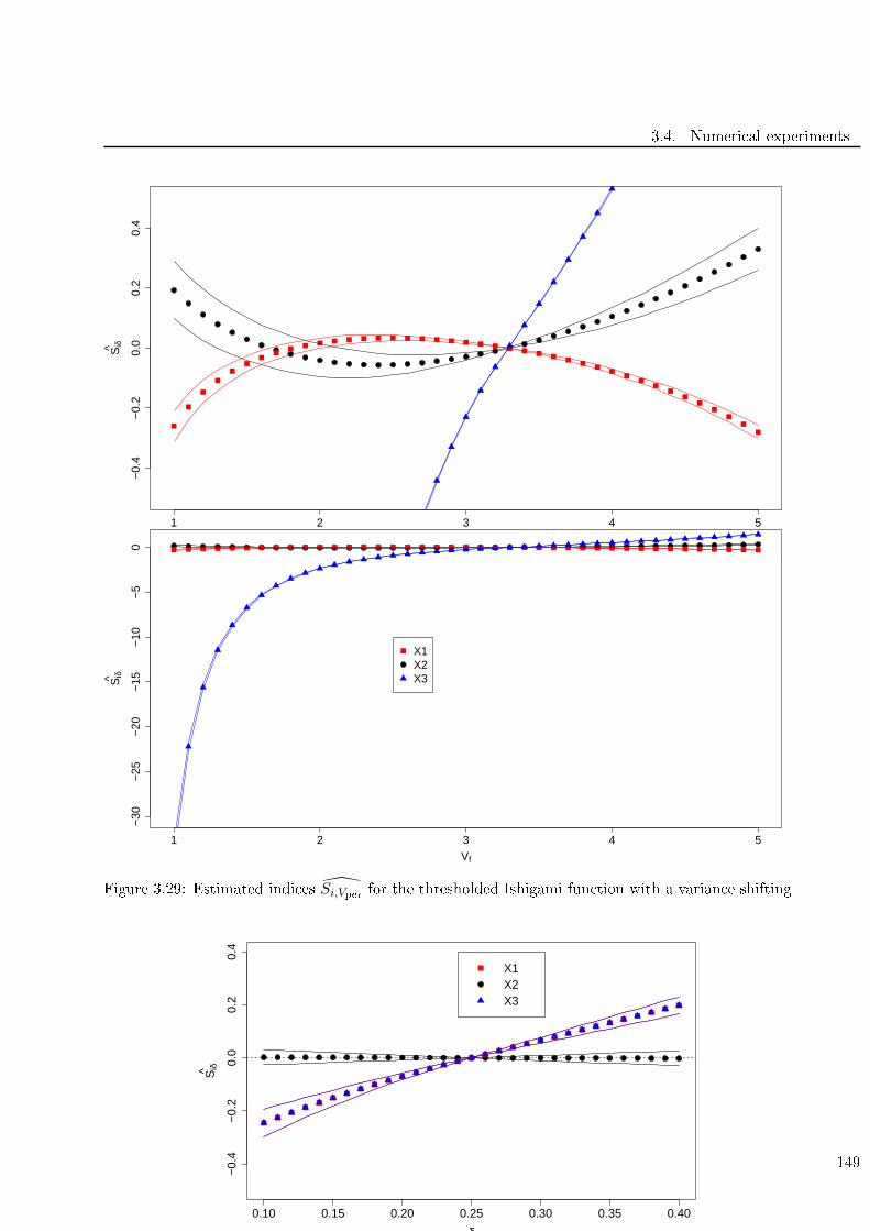
3.4. Numeri al experiments
1 2 3 4 5
−0.
4−
0.2
0.0
0.2
0.4
Siδ^
1 2 3 4 5
−30
−25
−20
−15
−10
−5
0
Vf
Siδ^
X1X2X3
Figure 3.29: Estimated indi es Si,Vper
for the thresholded Ishigami fun tion with a varian e shifting
0.10 0.15 0.20 0.25 0.30 0.35 0.40
−0.
4−
0.2
0.0
0.2
0.4
δ
Siδ^
X1X2X3
Figure 3.31:
st
quartile perturbation on the thresholded Ishigami test ase
149
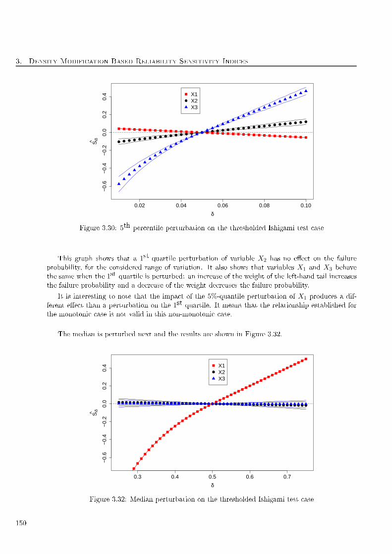
3. Density Modifi ation Based Reliability Sensitivity Indi es
0.02 0.04 0.06 0.08 0.10
−0.
6−
0.4
−0.
20.
00.
20.
4
δ
Siδ^
X1X2X3
Figure 3.30: 5th per entile perturbation on the thresholded Ishigami test ase
This graph shows that a 1st quartile perturbation of variable X2 has no ee t on the failure
probability, for the onsidered range of variation. It also shows that variables X1 and X3 behave
the same when the 1st quartile is perturbed: an in rease of the weight of the left-hand tail in reases
the failure probability and a de rease of the weight de reases the failure probability.
It is interesting to note that the impa t of the 5%-quantile perturbation of X1 produ es a dif-
ferent ee t than a perturbation on the 1st quartile. It means that the relationship established for
the monotoni ase is not valid in this non-monotoni ase.
The median is perturbed next and the results are shown in Figure 3.32.
0.3 0.4 0.5 0.6 0.7
−0.
6−
0.4
−0.
20.
00.
20.
4
δ
Siδ^
X1X2X3
Figure 3.32: Median perturbation on the thresholded Ishigami test ase
150
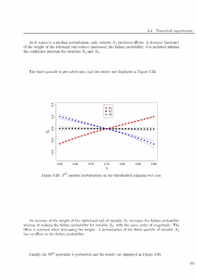
3.4. Numeri al experiments
As it omes to a median perturbation, only variable X1 produ es ee ts. A de rease (in rease)
of the weight of the left-hand tail redu es (in reases) the failure probability. 0 is in luded whithin
the onden e intervals for variables X2 and X3.
The third quartile is perturbed next and the results are displayed in Figure 3.33.
0.60 0.65 0.70 0.75 0.80 0.85 0.90
−0.
4−
0.2
0.0
0.2
0.4
δ
Siδ^
X1X2X3
Figure 3.33: 3rd quartile perturbation on the thresholded Ishigami test ase
An in rease of the weight of the right-hand tail of variable X1 in reases the failure probability
whereas it redu es the failure probability for variable X3, with the same order of magnitude. The
ee t is reversed when de reasing the weight. A perturbation of the third quartile of variable X2
has no ee t on the failure probability.
Finally, the 95th per entile is perturbed and the results are displayed in Figure 3.34.
151
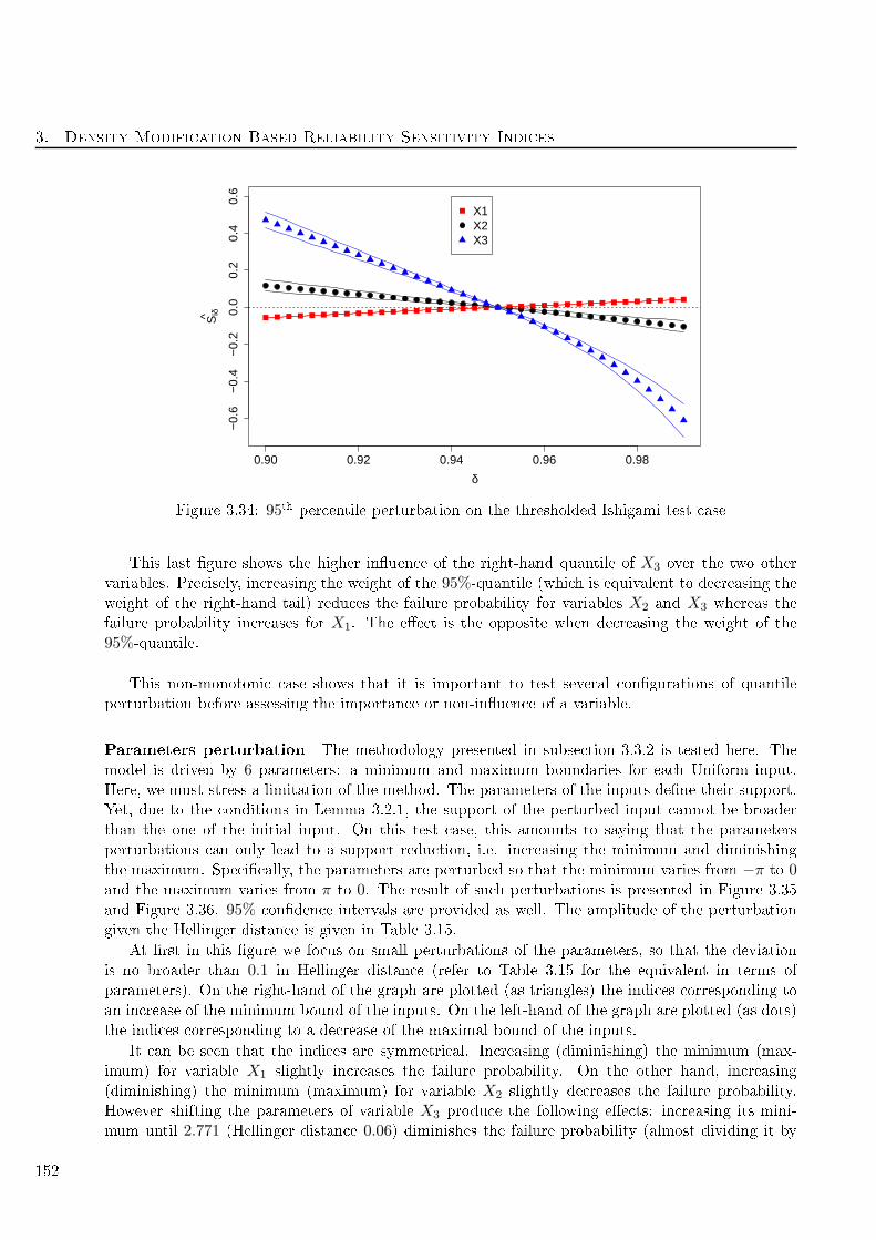
3. Density Modifi ation Based Reliability Sensitivity Indi es
0.90 0.92 0.94 0.96 0.98
−0.
6−
0.4
−0.
20.
00.
20.
40.
6
δ
Siδ^
X1X2X3
Figure 3.34: 95th per entile perturbation on the thresholded Ishigami test ase
This last gure shows the higher inuen e of the right-hand quantile of X3 over the two other
variables. Pre isely, in reasing the weight of the 95%-quantile (whi h is equivalent to de reasing the
weight of the right-hand tail) redu es the failure probability for variables X2 and X3 whereas the
failure probability in reases for X1. The ee t is the opposite when de reasing the weight of the
95%-quantile.
This non-monotoni ase shows that it is important to test several ongurations of quantile
perturbation before assessing the importan e or non-inuen e of a variable.
Parameters perturbation The methodology presented in subse tion 3.3.2 is tested here. The
model is driven by 6 parameters: a minimum and maximum boundaries for ea h Uniform input.
Here, we must stress a limitation of the method. The parameters of the inputs dene their support.
Yet, due to the onditions in Lemma 3.2.1, the support of the perturbed input annot be broader
than the one of the initial input. On this test ase, this amounts to saying that the parameters
perturbations an only lead to a support redu tion, i.e. in reasing the minimum and diminishing
the maximum. Spe i ally, the parameters are perturbed so that the minimum varies from −π to 0and the maximum varies from π to 0. The result of su h perturbations is presented in Figure 3.35
and Figure 3.36. 95% onden e intervals are provided as well. The amplitude of the perturbation
given the Hellinger distan e is given in Table 3.15.
At rst in this gure we fo us on small perturbations of the parameters, so that the deviation
is no broader than 0.1 in Hellinger distan e (refer to Table 3.15 for the equivalent in terms of
parameters). On the right-hand of the graph are plotted (as triangles) the indi es orresponding to
an in rease of the minimum bound of the inputs. On the left-hand of the graph are plotted (as dots)
the indi es orresponding to a de rease of the maximal bound of the inputs.
It an be seen that the indi es are symmetri al. In reasing (diminishing) the minimum (max-
imum) for variable X1 slightly in reases the failure probability. On the other hand, in reasing
(diminishing) the minimum (maximum) for variable X2 slightly de reases the failure probability.
However shifting the parameters of variable X3 produ e the following ee ts: in reasing its mini-
mum until 2.771 (Hellinger distan e 0.06) diminishes the failure probability (almost dividing it by
152
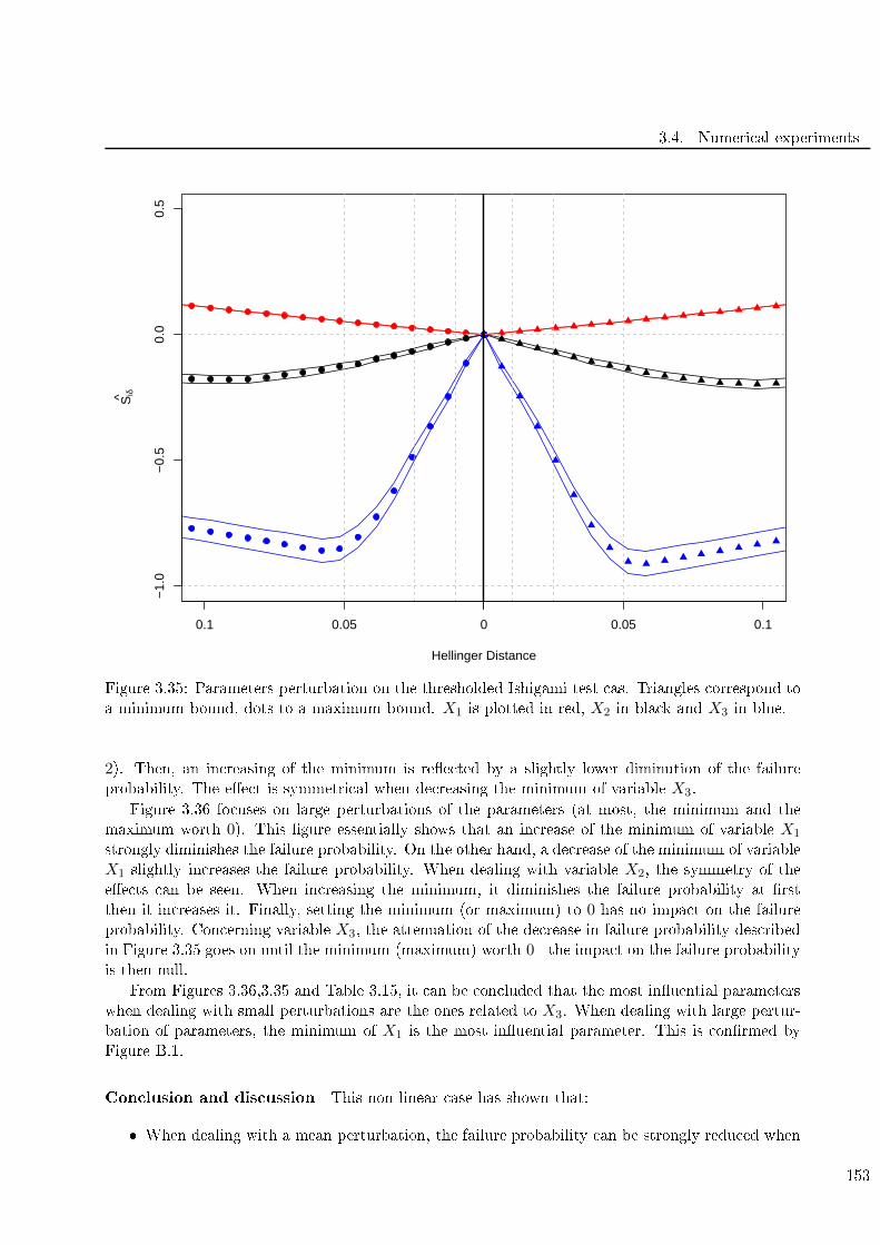
3.4. Numeri al experiments
−1.
0−
0.5
0.0
0.5
Hellinger Distance
Siδ^
0.1 0.05 0 0.05 0.1
Figure 3.35: Parameters perturbation on the thresholded Ishigami test as. Triangles orrespond to
a minimum bound, dots to a maximum bound. X1 is plotted in red, X2 in bla k and X3 in blue.
2). Then, an in reasing of the minimum is ree ted by a slightly lower diminution of the failure
probability. The ee t is symmetri al when de reasing the minimum of variable X3.
Figure 3.36 fo uses on large perturbations of the parameters (at most, the minimum and the
maximum worth 0). This gure essentially shows that an in rease of the minimum of variable X1
strongly diminishes the failure probability. On the other hand, a de rease of the minimum of variable
X1 slightly in reases the failure probability. When dealing with variable X2, the symmetry of the
ee ts an be seen. When in reasing the minimum, it diminishes the failure probability at rst
then it in reases it. Finally, setting the minimum (or maximum) to 0 has no impa t on the failure
probability. Con erning variable X3, the attenuation of the de rease in failure probability des ribed
in Figure 3.35 goes on until the minimum (maximum) worth 0 - the impa t on the failure probability
is then null.
From Figures 3.36,3.35 and Table 3.15, it an be on luded that the most inuential parameters
when dealing with small perturbations are the ones related to X3. When dealing with large pertur-
bation of parameters, the minimum of X1 is the most inuential parameter. This is onrmed by
Figure B.1.
Con lusion and dis ussion This non-linear ase has shown that:
When dealing with a mean perturbation, the failure probability an be strongly redu ed when
153
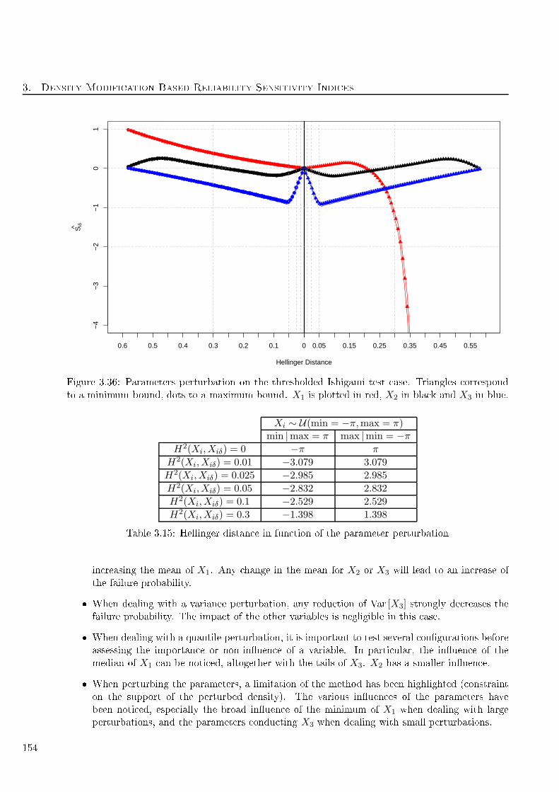
3. Density Modifi ation Based Reliability Sensitivity Indi es
−4
−3
−2
−1
01
Hellinger Distance
Siδ^
0.6 0.5 0.4 0.3 0.2 0.1 0 0.05 0.15 0.25 0.35 0.45 0.55
Figure 3.36: Parameters perturbation on the thresholded Ishigami test ase. Triangles orrespond
to a minimum bound, dots to a maximum bound. X1 is plotted in red, X2 in bla k and X3 in blue.
Xi ∼ U(min = −π,max = π)min |max = π max |min = −π
H2(Xi,Xiδ) = 0 −π π
H2(Xi,Xiδ) = 0.01 −3.079 3.079
H2(Xi,Xiδ) = 0.025 −2.985 2.985
H2(Xi,Xiδ) = 0.05 −2.832 2.832
H2(Xi,Xiδ) = 0.1 −2.529 2.529
H2(Xi,Xiδ) = 0.3 −1.398 1.398
Table 3.15: Hellinger distan e in fun tion of the parameter perturbation
in reasing the mean of X1. Any hange in the mean for X2 or X3 will lead to an in rease of
the failure probability.
When dealing with a varian e perturbation, any redu tion of Var [X3] strongly de reases the
failure probability. The impa t of the other variables is negligible in this ase.
When dealing with a quantile perturbation, it is important to test several ongurations before
assessing the importan e or non-inuen e of a variable. In parti ular, the inuen e of the
median of X1 an be noti ed, altogether with the tails of X3. X2 has a smaller inuen e.
When perturbing the parameters, a limitation of the method has been highlighted ( onstraint
on the support of the perturbed density). The various inuen es of the parameters have
been noti ed, espe ially the broad inuen e of the minimum of X1 when dealing with large
perturbations, and the parameters ondu ting X3 when dealing with small perturbations.
154
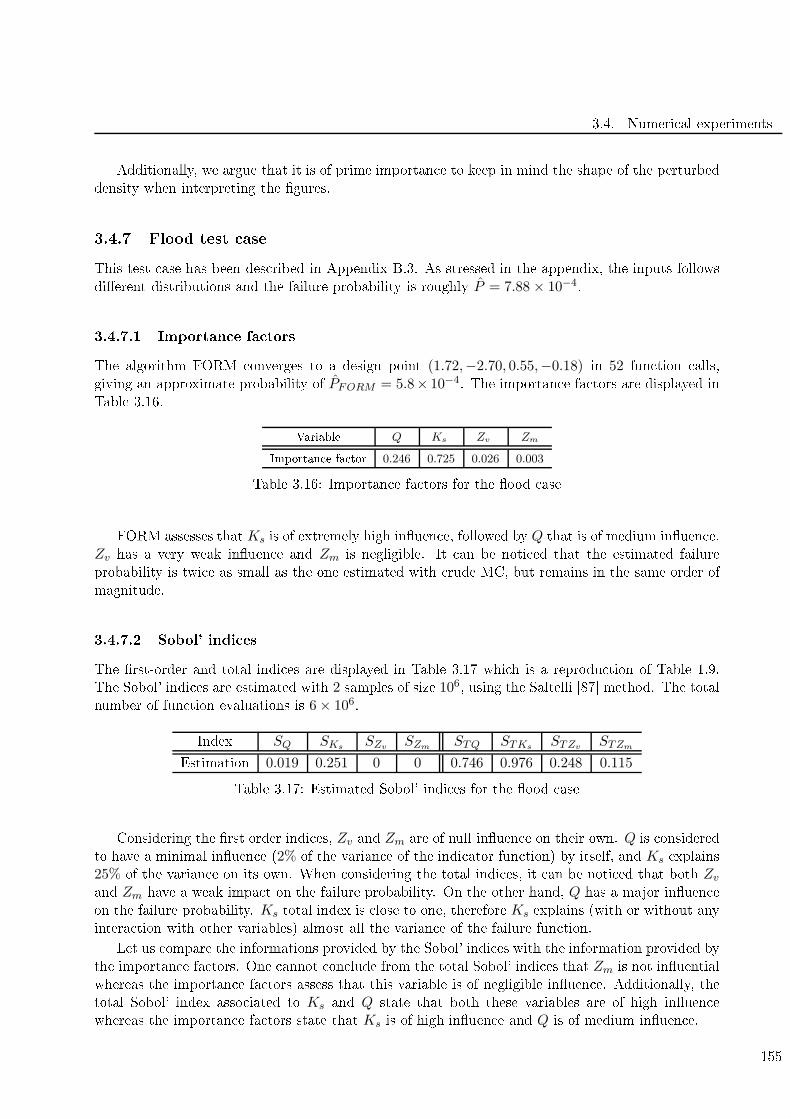
3.4. Numeri al experiments
Additionally, we argue that it is of prime importan e to keep in mind the shape of the perturbed
density when interpreting the gures.
3.4.7 Flood test ase
This test ase has been des ribed in Appendix B.3. As stressed in the appendix, the inputs follows
dierent distributions and the failure probability is roughly P = 7.88 × 10⁻⁴.
3.4.7.1 Importan e fa tors
The algorithm FORM onverges to a design point (1.72,−2.70, 0.55,−0.18) in 52 fun tion alls,
giving an approximate probability of PFORM = 5.8× 10⁻⁴. The importan e fa tors are displayed in
Table 3.16.
Variable Q Ks Zv Zm
Importan e fa tor 0.246 0.725 0.026 0.003
Table 3.16: Importan e fa tors for the ood ase
FORM assesses that Ks is of extremely high inuen e, followed by Q that is of medium inuen e.
Zv has a very weak inuen e and Zm is negligible. It an be noti ed that the estimated failure
probability is twi e as small as the one estimated with rude MC, but remains in the same order of
magnitude.
3.4.7.2 Sobol' indi es
The rst-order and total indi es are displayed in Table 3.17 whi h is a reprodu tion of Table 1.9.
The Sobol' indi es are estimated with 2 samples of size 106, using the Saltelli [87 method. The total
number of fun tion evaluations is 6× 10⁶.
Index SQ SKs SZv SZm STQ STKs STZv STZm
Estimation 0.019 0.251 0 0 0.746 0.976 0.248 0.115
Table 3.17: Estimated Sobol' indi es for the ood ase
Considering the rst order indi es, Zv and Zm are of null inuen e on their own. Q is onsidered
to have a minimal inuen e (2% of the varian e of the indi ator fun tion) by itself, and Ks explains
25% of the varian e on its own. When onsidering the total indi es, it an be noti ed that both Zv
and Zm have a weak impa t on the failure probability. On the other hand, Q has a major inuen e
on the failure probability. Ks total index is lose to one, therefore Ks explains (with or without any
intera tion with other variables) almost all the varian e of the failure fun tion.
Let us ompare the informations provided by the Sobol' indi es with the information provided by
the importan e fa tors. One annot on lude from the total Sobol' indi es that Zm is not inuential
whereas the importan e fa tors assess that this variable is of negligible inuen e. Additionally, the
total Sobol' index asso iated to Ks and Q state that both these variables are of high inuen e
whereas the importan e fa tors state that Ks is of high inuen e and Q is of medium inuen e.
155
3. Density Modifi ation Based Reliability Sensitivity Indi es
3.4.7.3 DMBRSI
Noti e that the dierent inputs follow various distributions, thus the question of "equivalent" per-
turbation arises. Due to this non-similarity of the distributions, only a (modied) mean shift, a
quantile shift and a parameter shift will be applied on this test ase. It has been dis ussed further
in 3.3.1.3. Additionally, a numeri al tri k is used to deal with trun ated distributions, as stressed in
Appendix D.4.
Mean shifting The hoi e has been made to shift the mean relatively to the standard deviation,
hen e in luding the spread of the various inputs in their respe tive perturbation. So for any input,
the original distribution is perturbed so that its mean is the original's one plus δ times its standard
deviation, δ ranging from −1 to 1 with 40 points.
Figure 3.37: Estimated indi es Siδ for the ood ase with a mean perturbation
Figure 3.37 assesses that an in reasing of the mean of the inputs in reases the failure probability
slightly for Zv, strongly for Q, and diminishes it slightly for Zm and strongly for Ks. This goes
the opposite way when de reasing the mean. In terms of absolute modi ation, Ks and Q are of
same magnitude, even if Ks has a slightly stronger impa t. On the other hand, the ee ts of mean
perturbation on Zm and Zv are negligible. The CI asso iated to Q and Ks are well separated from
the others, ex ept in a δ = −.3 to .3 zone. The onden e intervals asso iated to Zv and Zm
overlap. Thus even though the indi es seem to have dierent values, it is not possible to on lude
with ertainty about the inuen e of those variables.
Quantile shifting The rst quantile to be perturbed is the extreme left-hand tail, namely the
5%-quantile. The result of su h a perturbation for all the variables is plotted in Figure 3.38.
156

3.4. Numeri al experiments
Figure 3.38: 5th per entile perturbation on the ood ase
When it omes to a left-hand tail perturbation, the inuen e of Ks over the three other variables
is preponderant. In parti ular, a redu tion of the weight of the 5th per entile to 0.015 leads to a
division by 3 of the failure probability.
The 1st quartile is then perturbed and the results are plotted in Figure 3.39.
Figure 3.39: 1st quartile perturbation on the ood ase
On e again when perturbing the left-hand tail, the inuen e of Ks is larger than the inuen e
of the other variables.
The median of the input distributions is then perturbed, the resulting indi es are plotted in
Figure 3.40.
The inuen e of KS is weaker than in the two previous gures, as Ks and Q have a similar
157
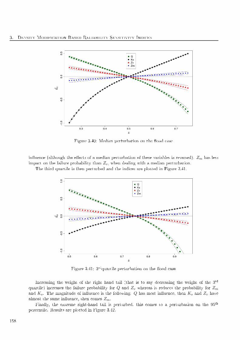
3. Density Modifi ation Based Reliability Sensitivity Indi es
Figure 3.40: Median perturbation on the ood ase
inuen e (although the ee ts of a median perturbation of these variables is reversed). Zm has less
impa t on the failure probability than Zv, when dealing with a median perturbation.
The third quartile is then perturbed and the indi es are plotted in Figure 3.41.
Figure 3.41: 3rdquartile perturbation on the ood ase
In reasing the weight of the right hand tail (that is to say de reasing the weight of the 3rd
quartile) in reases the failure probability for Q and Zv whereas it redu es the probability for Zm
and Ks. The magnitude of inuen e is the following: Q has most inuen e, then Ks and Zv have
almost the same inuen e, then omes Zm.
Finally, the extreme right-hand tail is perturbed, this omes to a perturbation on the 95th
per entile. Results are plotted in Figure 3.42.
158
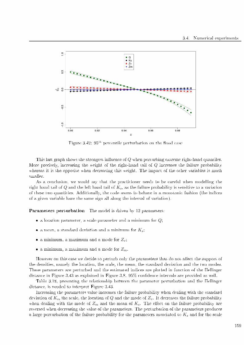
3.4. Numeri al experiments
Figure 3.42: 95th per entile perturbation on the ood ase
This last graph shows the strongest inuen e of Q when perturbing extreme right-hand quantiles.
More pre isely, in reasing the weight of the right-hand tail of Q in reases the failure probability
whereas it is the opposite when de reasing this weight. The impa t of the other variables is mu h
smaller.
As a on lusion, we would say that the pra titioner needs to be areful when modelling the
right-hand tail of Q and the left-hand tail of Ks, as the failure probability is sensitive to a variation
of these two quantities. Additionally, the ode seems to behave in a monotoni fashion (the indi es
of a given variable have the same sign all along the interval of variation).
Parameters perturbation The model is driven by 12 parameters:
a lo ation parameter, a s ale parameter and a minimum for Q;
a mean, a standard deviation and a minimum for Ks;
a minimum, a maximum and a mode for Zv;
a minimum, a maximum and a mode for Zm.
However on this ase we de ide to perturb only the parameters that do not ae t the support of
the densities, namely the lo ation, the s ale, the mean, the standard deviation and the two modes.
These parameters are perturbed and the estimated indi es are plotted in fun tion of the Hellinger
distan e in Figure 3.43 as explained in Figure 3.8. 95% onden e intervals are provided as well.
Table 3.18, presenting the relationship between the parameter perturbation and the Hellinger
distan e, is needed to interpret Figure 3.43.
In reasing the parameters value in reases the failure probability when dealing with the standard
deviation of Ks, the s ale, the lo ation of Q and the mode of Zv. It de reases the failure probability
when dealing with the mode of Zm and the mean of Ks. The ee t on the failure probability are
reversed when de reasing the value of the parameters. The perturbation of the parameters produ es
a large perturbation of the failure probability for the parameters asso iated to Ks and for the s ale
159
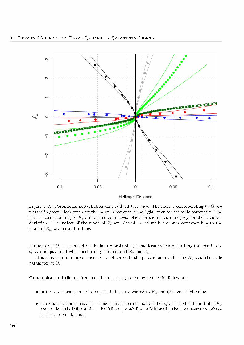
3. Density Modifi ation Based Reliability Sensitivity Indi es
−3
−2
−1
01
23
Hellinger Distance
Siδ^
0.1 0.05 0 0.05 0.1
Figure 3.43: Parameters perturbation on the ood test ase. The indi es orresponding to Q are
plotted in green: dark green for the lo ation parameter and light green for the s ale parameter. The
indi es orresponding to Ks are plotted as follows: bla k for the mean, dark grey for the standard
deviation. The indi es of the mode of Zv are plotted in red while the ones orresponding to the
mode of Zm are plotted in blue.
parameter of Q. The impa t on the failure probability is moderate when perturbing the lo ation of
Q, and is quasi-null when perturbing the modes of Zv and Zm.
It is thus of prime importan e to model orre tly the parameters ondu ting Ks, and the s ale
parameter of Q.
Con lusion and dis ussion On this test ase, we an on lude the following:
In terms of mean perturbation, the indi es asso iated to Ks and Q have a high value.
The quantile perturbation has shown that the right-hand tail of Q and the left-hand tail of Ks
are parti ularly inuential on the failure probability. Additionally, the ode seems to behave
in a monotoni fashion.
160

3.5. Improving the DMBRSI estimation
Xi ∼ GT (lo = 1013, s ale = 558,min = 0) Xi ∼ NT (µ = 30, σ = 7.5,min = 1)lo |s ale = 558,min = 0 s ale|lo = 1013,min = 0 µ|σ = 7.5,min = 1 σ|µ = 30,min = 1
H2(Xi, Xiδ) = 0 1013 558 30 7.5
H2(Xi, Xiδ) = 0.01 893/1128 478/661 28.49/31.50 6.51/8.65
H2(Xi, Xiδ) = 0.025 820/1194 437/736 27.62/32.38 5.99/9.42
H2(Xi, Xiδ) = 0.05 732/1269 395/838 26.62/33.38 5.44/10.40
H2(Xi, Xiδ) = 0.1 590/1377 342/1021 25.19/34.81 4.73/12.08
Xi ∼ T (a = 49, b = 51, c = 50) Xi ∼ T (a = 54, b = 56, c = 55)c|a = 49, b = 51 c|a = 54, b = 56
H2(Xi, Xiδ) = 0 50 55
H2(Xi, Xiδ) = 0.01 49.79/50.21 54.79/55.21
H2(Xi, Xiδ) = 0.025 49.65/50.35 54.65/55.35
H2(Xi, Xiδ) = 0.05 49.49/50.51 49.49/50.51
H2(Xi, Xiδ) = 0.1 49.26/50.74 49.26/50.74
Table 3.18: Hellinger distan e in fun tion of the parameter perturbation
The parameters perturbation has demonstrated that the parameters of Ks and the s ale pa-
rameter of Q impa t most the output.
This more realisti test ase has shown that the DMBRSI provide several omplementary infor-
mations.
3.5 Improving the DMBRSI estimation
This hapter has presented a new SA methodology based on density perturbations. For the sake of
simpli ity, we have onsidered a rude Monte-Carlo framework. However, this onsideration might
be unrealisti when dealing with real appli ation ases where the number of fun tion alls is limited.
We thus propose in this Se tion to improve the DMBRSI estimation with importan e sampling
(Se tion 3.5.1) and with subset simulation (Se tion 3.5.2).
3.5.1 Coupling DMBRSI with importan e sampling
3.5.1.1 Estimating Pf with IS
Denoting f a d−dimensional importan e density su h that Supp(f) ⊇ Supp(f). Suppose one has
an i.i.d. N-sample with pdf f , denoted xnwith n going from 1 to N .
The failure probability Pf an be estimated with Importan e Sampling method (see Se tion
1.2.1.3) and the asso iated estimator with N fun tion alls is:
PNIS =1
N
N∑
n=1
1G(xn)<0f(xn)
f(xn). (3.32)
One an show that:
Var
[PNIS
]=
1
NVarf
[1G(X)<0
f(X)
f(X)
]=
1
N
(
1G(x)<0f2(x)
f(x)dx− P 2
f
)(3.33)
NB : the varian e redu tion from IS is not straightforward, one should ompare Varf
[1G(X)<0
f(X)
f(X)
]
and Varf
[1G(X)<0
]to on lude, as stressed in Se tion 1.2.1.3.
161
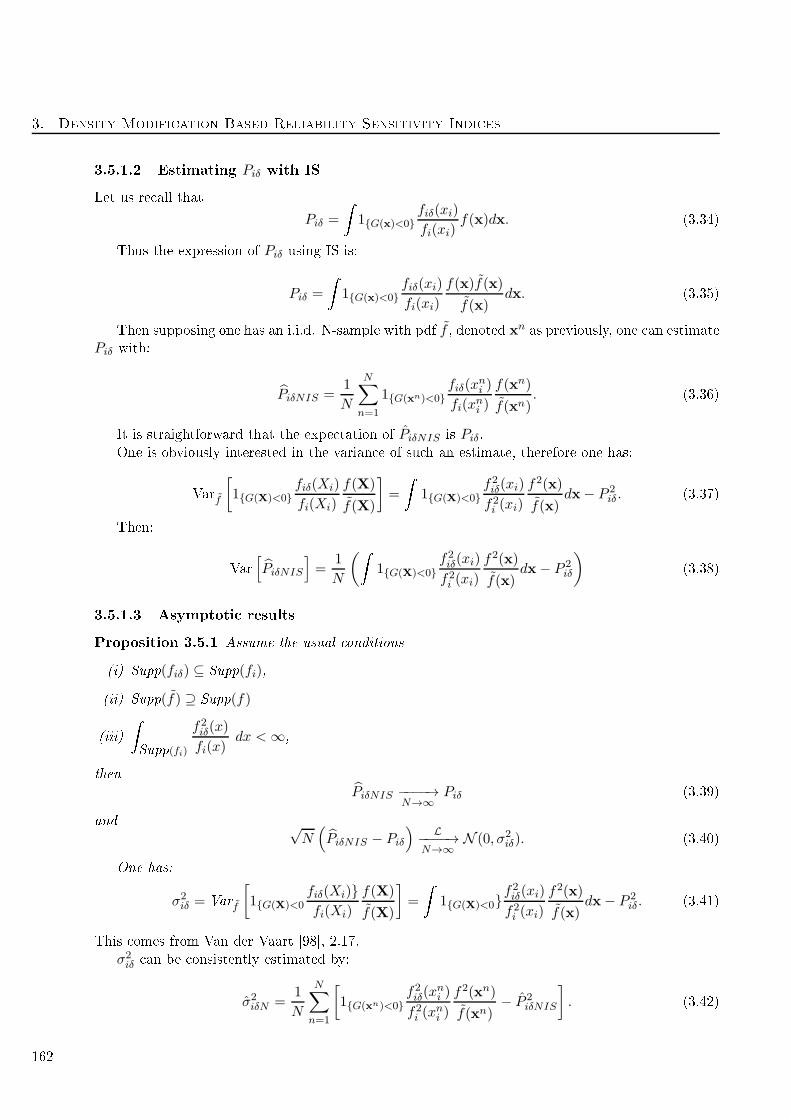
3. Density Modifi ation Based Reliability Sensitivity Indi es
3.5.1.2 Estimating Piδ with IS
Let us re all that
Piδ =
1G(x)<0fiδ(xi)
fi(xi)f(x)dx. (3.34)
Thus the expression of Piδ using IS is:
Piδ =
1G(x)<0fiδ(xi)
fi(xi)
f(x)f(x)
f(x)dx. (3.35)
Then supposing one has an i.i.d. N-sample with pdf f , denoted xnas previously, one an estimate
Piδ with:
PiδNIS =1
N
N∑
n=1
1G(xn)<0fiδ(x
ni )
fi(xni )
f(xn)
f(xn). (3.36)
It is straightforward that the expe tation of PiδNIS is Piδ.
One is obviously interested in the varian e of su h an estimate, therefore one has:
Varf
[1G(X)<0
fiδ(Xi)
fi(Xi)
f(X)
f(X)
]=
1G(X)<0f2iδ(xi)
f2i (xi)
f2(x)
f(x)dx− P 2
iδ . (3.37)
Then:
Var
[PiδNIS
]=
1
N
(
1G(X)<0f2iδ(xi)
f2i (xi)
f2(x)
f(x)dx− P 2
iδ
)(3.38)
3.5.1.3 Asymptoti results
Proposition 3.5.1 Assume the usual onditions
(i) Supp(fiδ) ⊆ Supp(fi),
(ii) Supp(f) ⊇ Supp(f)
(iii)
Supp(fi)
f2iδ(x)
fi(x)dx <∞,
then
PiδNIS −−−−→N→∞
Piδ (3.39)
and √N(PiδNIS − Piδ
) L−−−−→N→∞
N (0, σ2iδ). (3.40)
One has:
σ2iδ = Varf
[1G(X)<0
fiδ(Xi)fi(Xi)
f(X)
f(X)
]=
1G(X)<0f2iδ(xi)
f2i (xi)
f2(x)
f(x)dx− P 2
iδ. (3.41)
This omes from Van der Vaart [98, 2.17.
σ2iδ an be onsistently estimated by:
σ2iδN =1
N
N∑
n=1
[1G(xn)<0
f2iδ(xni )
f2i (xni )
f2(xn)
f(xn)− P 2
iδNIS
]. (3.42)
162
3.5. Improving the DMBRSI estimation
Proposition 3.5.2
√N
(PNIS
PiδNIS−(Pf
Piδ
))L−−−−→
N→∞N (0,ΣiδIS) (3.43)
where:
ΣiδIS =
1G(X)<0f2(x)
f(x)dx− P 2
f
1G(X)<0fiδ(xi)
fi(xi)f2(x)
f(x)dx− PfPiδ
1G(X)<0fiδ(xi)
fi(xi)f2(x)
f(x)dx− PfPiδ
1G(X)<0f2iδ(xi)
f2i (xi)f2(x)
f(x)dx− P 2
iδ
. (3.44)
This omes a ording to Van der Vaart [98, 2.18.
We propose the following estimator for ΣiδIS :
ΣNiδIS =
1
N
(N∑
n=1
1G(xn)<0f2(xn)
f(xn)
)− P 2
NIS
1
N
(N∑
n=1
1G(xn)<0f2(xn)
f(xn)
fiδ(xi)
fi(xi)
)− PNISPiδNIS
1
N
(N∑
n=1
1G(xn)<0f2(xn)
f(xn)
fiδ(xi)
fi(xi)
)
− PNISPiδNIS1
N
(N∑
n=1
1G(xn)<0f2(xn)
f(xn)
f2iδ(xi)
f2i (xi)
)
− P 2iδNIS
.
(3.45)
Proposition 3.5.3 Introdu ing the fun tion s(x, y) =( yx − 1
)1y>x +
(1− x
y
)1x>y, denoting:
(i) Siδ = s(Pf , Piδ)
(ii) SNiδIS = s(PNIS , PiδNIS).
As s is dierentiable in (P,Piδ) (see Proposition 3.2.2), one has:
√N(SNiδIS − Siδ
)L−−−−→
N→∞N (0, dTs ΣiδISds). (3.46)
The proof lies in Theorem 3.1 in Van der Vaart [98.
3.5.2 Coupling DMBRSI with subset simulation
We refer to Se tion 1.2.3 for more details about subset simulation. The aim of the urrent se tion
is to show that it is possible to use the results of a subset simulation algorithm to estimate the
quantity Piδ, the perturbed failure probability (see Equation 3.1).
Let us imagine, for the sake of larity, a two-step subset where the levels are xed in advan e.
Let us denote by A, B, 0 the thresholds to ross at the algorithm's steps, with A > B > 0.
We have PA =
1G(x)≤Af(x)dx; PB =
1G(x)≤Bf(x)dx and Pf =
1G(x)≤0f(x)dx.
Additionally, let us remind that
Piδ =
1G(x)≤0fiδ(xi)
fi(xi)f(x)dx = E[1G(Xiδ)≤0] = P (G(Xiδ) ≤ 0) (3.47)
The algorithm starts with N points x(j),1, j = 1 . . . N distributed a ording to f , the original
density. PA an be estimated by:
PA =1
N
∑1G(x(j),1)≤A (3.48)
163
3. Density Modifi ation Based Reliability Sensitivity Indi es
where one has:
E
[PA
]=
1G(x)≤Af(x)dx = PA. (3.49)
Then, after a mutation/sele tion step, one has N points x(j),2, j = 1 . . . N distributed a ording
to f(x|A) = 1G(x)≤Af(x)
PA. The following estimator is proposed for PB|A =
1G(x)≤B|G(x)≤Af(x)dx =
1G(x)≤B∩G(x)≤Af(x)dx
1G(x)≤Af(x)dx=
1G(x)≤Bf(x)dx
1G(x)≤Af(x)dx= PB
PA:
PB
PA=
1
N
∑1G(x(j),2)≤B. (3.50)
One has:
E
[PB
PA
]=
1G(x)≤B1G(x)≤Af(x)
PAdx =
1G(x)≤Bf(x)dx
PA=PB
PA(3.51)
After a se ond mutation/sele tion step, one has N points x(j),3, j = 1 . . . N distributed a ording
to f(x|B) =1G(x)≤Bf(x)
PB. The following estimator is proposed for P0|B =
1G(x)≤0|G(x)≤Bf(x)dx:
P0|B =1
N
∑1G(x(j),3)≤0. (3.52)
One an he k that:
E
[P0|B
]=
1G(x)≤01G(x)≤Bf(x)
PBdx =
1G(x)≤0f(x)dx
PB=
P
PB(3.53)
Finally, Pf = PA × PB|A × P0|B,A. Yet B ⇒ A thus P0|B,A = P0|B . P is estimated by:
P = PAPB|AP0|B
Considering PA ,PB|A et P0|B as realisation of independent random variables
1
one has:
E
[P]= E
[PA
]E
[PB|A
]E
[P0|B
]= PA × PB
PA× P
PB= P.
Then, it is observed that:
Piδ =Piδ
PB
PB
PAPA
Considering the N points x(j),3, j = 1..N distributed a ording to f(x/B) =1G(x)≤Bf(x)
PB.
Piδ
PB
is estimated by:
Piδ
PB=
1
N
∑1G(x(j),3)≤0
fiδ(x(j),3i )
fi(x(j),3i )
.
One an he k that:
E
[Piδ
PB
]=
1G(x)≤01G(x)≤Bf(x)
PB
fiδ(xi)
fi(xi)dx =
1
PB
1G(x)≤0fiδ(xi)
fi(xi)f(x)dx =
Piδ
PB.
1
This is not the ase in reality, the mutation step is just performed several times
164
3.6. Dis ussion and on lusion
Considering
Piδ
PB,
PB
PAet PA as realisation of independent random variables
2
one has:
E
[Piδ
]= E
[Piδ
PB
]E
[PB
PA
]E
[PA
]= Piδ .
Con lusion To ouple DMBRSI and subset simulation, one just has to perturb the points oming
from the last step of the subset. However, the varian e of Piδ is intra table so far. This will be the
obje t of further resear hes.
3.6 Dis ussion and on lusion
3.6.1 Con lusion on the DMBRSI method
The method presented in this hapter gives relevant omplementary information in addition of
traditional SA methods applied to a reliability problem. Traditional SA methods provide variable
ranking, whereas the proposed method provides an indi ation on the variation in the probability
of failure given the variation of parameter δ. This is useful when the pra titioner is interested on
whi h ongurations of the problem lead to an in rease of the failure probability. This might also
be used to assess the onservatism of a problem, if every variations of the input lead to de rease in
the probability of failure. Additionally, it has three advantages:
the ability for the user to set the most adapted onstraints onsidering his/her problem/obje tive.
The MC framework allowing to use previously done fun tion alls, thus limiting the CPU ost
of the SA, and allowing the user to test several perturbations.
They are easy to interpret.
We argue that with an adapted perturbation, this method an fulll the presented reliability engi-
neer's obje tive (see Se tion 3.3.3 for further dis ussions on this topi ). From this point of view, the
DMBRSI are a good alternative to FORM/SORM's importan e fa tors (as they an provide wrong
results, see the Ishigami ase) and to Sobol' indi es (as they are ostly and non-informative).
3.6.2 Equivalent perturbation
The question of "equivalent" perturbation arises from ases where all inputs are not identi ally
distributed. Indeed, problems may emerge when some inputs are dened on innite intervals and
when other inputs are dened on nite intervals (su h as uniform distributions). We have proposed
three ways to deal with these problems:
perform a mean perturbation relatively to the standard deviation, hen e in luding the spread
of the various inputs in their respe tive perturbation;
perform a quantile shifting;
perform a parameters perturbation.
2
This is not the ase in reality
165
3. Density Modifi ation Based Reliability Sensitivity Indi es
3.6.3 Support perturbation
In most examples given throughout this hapter, the perturbations of the inputs left the support
of those variables unperturbed. However, a support modi ation has been tested on the Ishigami
ase where the parameters dening the support have been perturbed. Yet, we stress that given the
estimation method (reverse importan e sampling), it is mandatory that the support of the perturbed
density is in luded in the support of the original density. Thus one annot perturb the inputs so
that the perturbed support is wider than the original one.
3.6.4 Further work
Most of the further work will be devoted to adapting the estimator of the indi es Siδ in term of
varian e redu tion and of number of fun tion alls. Further work will be made with importan e sam-
pling methods (test the proposed estimators). The adaptation of estimators using subset simulation
must also be done.
A perturbation based on an entropy onstraint might also be proposed. The dierential entropy
of a distribution an be seen as a quanti ation of un ertainty (Auder et al. [6). Thus an example
of (non-linear) onstraint on the entropy an be:
−
fiδ(x) log fiδ(x)dx = −δ
fi(x) log fi(x)dx.
Yet further omputations have to be made to obtain a tra table solution of the KL minimization
problem under the above onstraint.
Another avenue worth exploring would be to hange the metri s/divergen es. That would amount
to hange the D in equation 3.9 ( hoi e was made to take KLD); and to take another distan e than
Hellinger's in the parameter perturbation ontext. This has to be tested.
3.6.5 A knoweldgements
We thank all the oauthors of the paper [63 for their help on this hapter. Part of this work has been
ba ked by Fren h National Resear h Agen y (ANR) through COSINUS program (proje t COSTA
BRAVA noANR-09-COSI-015). We also thank Dr. Daniel Busby (IFP EN) for several dis ussions
and Emmanuel Remy (EDF R&D) for proofreading. We also thank two anonymous reviewers for
their helpful omments. All the statisti al parts of this work have been performed within the R
environment, in luding the mistral and sensitivity pa kages.
166
Chapter 4
Appli ation to the CWNR ase
4.1 Introdu tion
This fourth hapter presents the appli ation of some of the developed methods to the CWNR ase.
This numeri al model has been presented in the outline of the thesis, page 24. Remind that this
bla k-box model provided the initial motivation for this thesis.
The software interfa ing is done using the Open TURNS [2 software that manages the probabilist
part of the analysis. A wrapper alls the model when ne essary. Con erning the sensitivity analysis
part, post-pro essing of the data obtained is done using the R software.
In this thesis, fo us has been set on SA methods that are separated from the sampling step (see
Chapter 2), Chapter 3), thus the separation between the estimation of Pf and the sensitivity analysis.
To estimate Pf , the failure probability, FORM (see Se tion 1.2.2.2) method and rude Monte-Carlo
(see Se tion 1.2.1.1) have been used. Crude Monte-Carlo is onsidered to be the referen e method
in this hapter. Importan e sampling (see Se tion 1.2.1.3) was available but was not used due to
the la k of knowledge to set the importan e densities. Subset simulation (see Se tion 1.2.3) was
also available but was not used due to the fa t that the Open TURNS module only provides an
estimation for Pf and not the sampling points.
The sensitivity analysis part then fo uses on three methods: rst, importan e fa tors (see Se tion
1.3.2.2) are derived from the FORM sampling. Then, random forests (see Se tion 2.2) are built on
the MC sample and sensitivity measures are obtained. Finally, DMBRSI (see Chapter 3) are used.
Several perturbations (mean, quantile and parameters) are proposed.
Sobol' indi es (see Se tion 1.4) are not tested in this hapter due to the limited information
provided and the high omputational ost. δSSi (Ak) indi es (see Se tion 2.3) are not used in this
hapter sin e a sampling s heme from subset simulation was not available.
This hapter is divided in three main se tions, fo using respe tively on random input of dimension
3 (Se tion 4.2), dimension 5 (Se tion 4.3) and dimension 7 (Se tion 4.4). Noti e that the smaller
the dimension of the input, the more penalizing the ase (sin e non-probabilised variables are set to
penalizing values). Thus the failure probability diminishes as the dimensionality growths. A nal
se tion (Se tion 4.5) on ludes.
4.2 Three variables ase
In this rst se tion, three variables are probabilised. Table 1 is partially reprodu ed in Table 4.1 to
indi ate whi h distributions follow the variables. Table A.1 is a reminder of the inputs' densities.
167

4. Appli ation to the CWNR ase
Random var. Distribution Parameters
Thi kness (m) Uniform a = 0.0075, b = 0.009
h (m) Weibull a = 0.02, s ale= 0.00309, shape= 1.8
Ratio height/length Lognormal a = 0.02, ln (b) = −1.53, ln (c) = 0.55
Table 4.1: Distributions of the random physi al variables of the CWNR model - 3 variables
4.2.1 Estimating Pf
4.2.1.1 Crude Monte-Carlo
A Crude Monte-Carlo (MC) estimation has been performed, with a sample of size 10000. 683 points
were failing points thus the failure probability is estimated by:
Pf = 0.0683.
This will be onsidered as the referen e result. The sampling s heme will be used to build random
forests (Se tion 4.2.2.1) and DMBRSI (Se tion 4.2.2.2).
4.2.1.2 FORM
FORM has been used. 52 fun tion alls have been done. However the estimated failure probability
is here of:
PFORM = 3.19 × 10⁻¹⁶,
whi h is several orders of magnitude beneath the referen e value. The results of FORM are not
trustworthy in this ase, therefore no sensitivity analysis will be performed with FORM in this ase.
Noti e that the user is not warned that the FORM results are wrong. This is a major drawba k of
this te hnique.
4.2.2 Sensitivity Analysis
4.2.2.1 Random Forests
The methodology presented in Se tion 2.2 is used along this se tion. A forest of 500 trees is tted
on the MC sample. The referen e value ⌊√d⌋ is used as the number of variables randomly sele ted
at ea h step. In this ase, it means that 1 variable is sele ted as d = 3.
Variable Thi kness h Ratio
Index 0.01448048 0.10574811 0.02529668
Table 4.2: MDA index - 3 variables
MDA From Table 4.2, it an be inferred that the most inuential variable is h, with 5 times as
mu h inuen e as the se ondly important variable, namely the ratio. Finally omes the thi kness
with an index twi e as small as the one of the ratio. However from the numeri al results of Se tion
2.2, it an be stated that the thi kness has some inuen e on its own, a ording to the MDA indi es.
168
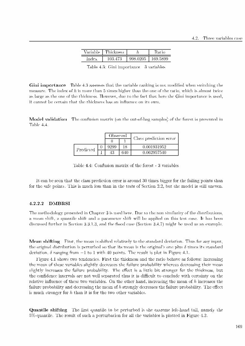
4.2. Three variables ase
Variable Thi kness h Ratio
Index 103.473 998.0205 169.5899
Table 4.3: Gini importan e - 3 variables
Gini importan e Table 4.3 assesses that the variable ranking is not modied when swit hing the
measure. The index of h is more than 5 times higher than the one of the ratio, whi h is almost twi e
as large as the one of the thi kness. However, due to the fa t that here the Gini importan e is used,
it annot be ertain that the thi kness has an inuen e on its own.
Model validation The onfusion matrix (on the out-of-bag samples) of the forest is presented in
Table 4.4.
Observed
Class predi tion error
0 1
Predi ted
0 9299 18 0.0019319521 43 640 0.062957540
Table 4.4: Confusion matrix of the forest - 3 variables
It an be seen that the lass predi tion error is around 30 times bigger for the failing points than
for the safe points. This is mu h less than in the tests of Se tion 2.2, but the model is still uneven.
4.2.2.2 DMBRSI
The methodology presented in Chapter 3 is used here. Due to the non-similarity of the distributions,
a mean shift, a quantile shift and a parameter shift will be applied on this test ase. It has been
dis ussed further in Se tion 3.3.1.3, and the ood ase (Se tion 3.4.7) might be used as an example.
Mean shifting First, the mean is shifted relatively to the standard deviation. Thus for any input,
the original distribution is perturbed so that its mean is the original's one plus δ times its standard
deviation, δ ranging from −1 to 1 with 40 points. The result is plot in Figure 4.1.
Figure 4.1 shows two tenden ies. First the thi kness and the ratio behave as follows: in reasing
the mean of these variables slightly de reases the failure probability whereas de reasing their mean
slightly in reases the failure probability. The ee t is a little bit stronger for the thi kness, but
the onden e intervals are not well separated thus it is di ult to on lude with ertainty on the
relative inuen e of these two variables. On the other hand, in reasing the mean of h in reases the
failure probability and de reasing the mean of h strongly de reases the failure probability. The ee t
is mu h stronger for h than it is for the two other variables.
Quantile shifting The rst quantile to be perturbed is the extreme left-hand tail, namely the
5%-quantile. The result of su h a perturbation for all the variables is plotted in Figure 4.2.
169
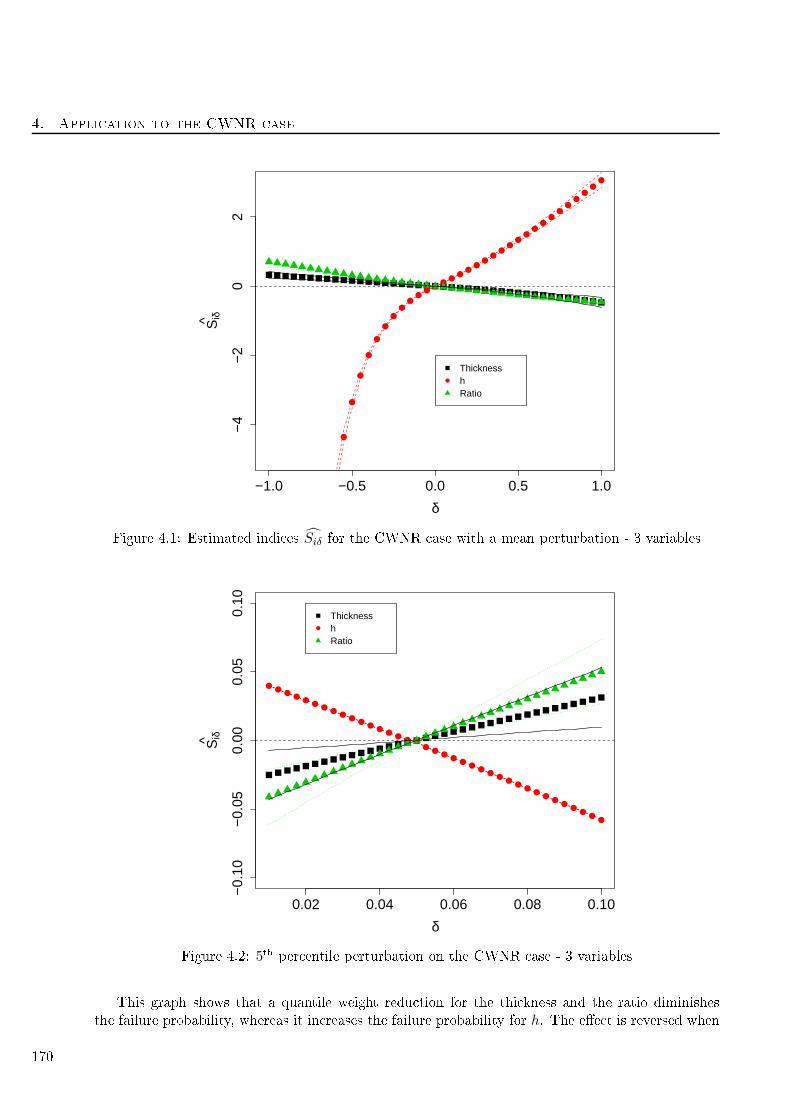
4. Appli ation to the CWNR ase
−1.0 −0.5 0.0 0.5 1.0
−4
−2
02
δ
Siδ^
ThicknesshRatio
Figure 4.1: Estimated indi es Siδ for the CWNR ase with a mean perturbation - 3 variables
0.02 0.04 0.06 0.08 0.10
−0.
10−
0.05
0.00
0.05
0.10
δ
Siδ^
ThicknesshRatio
Figure 4.2: 5th per entile perturbation on the CWNR ase - 3 variables
This graph shows that a quantile weight redu tion for the thi kness and the ratio diminishes
the failure probability, whereas it in reases the failure probability for h. The ee t is reversed when
170
4.2. Three variables ase
in reasing the weight of the quantile. The inuen e is of the same order of magnitude for the three
variables, with a slightly smaller inuen e for the ratio. However, the onden e intervals for the
ratio and the thi kness are not well separated.
The 1st quartile is then perturbed and the results are plotted in Figure 4.3.
0.10 0.15 0.20 0.25 0.30 0.35 0.40
−0.
2−
0.1
0.0
0.1
0.2
δ
Siδ^
ThicknesshRatio
Figure 4.3: 1st quartile perturbation on the CWNR ase - 3 variables
When perturbing less extreme values of the left-hand tail, the results are similar. In parti ular,
the inuen es are of the same order of magnitude yet h has a larger inuen e than the thi kness,
whi h has a larger inuen e than the ratio. The onden e intervals are separated.
The median of the input distributions is then perturbed, the resulting indi es are plotted in
Figure 4.4.
When perturbing the median, tenden ies are similar to the two previous graphs. The inuen e
of h is larger than the inuen e of the other variables. The thi kness has a larger inuen e than the
ratio. Conden e intervals are well separated.
The third quartile is then perturbed and the indi es are plotted in Figure 4.5.
171
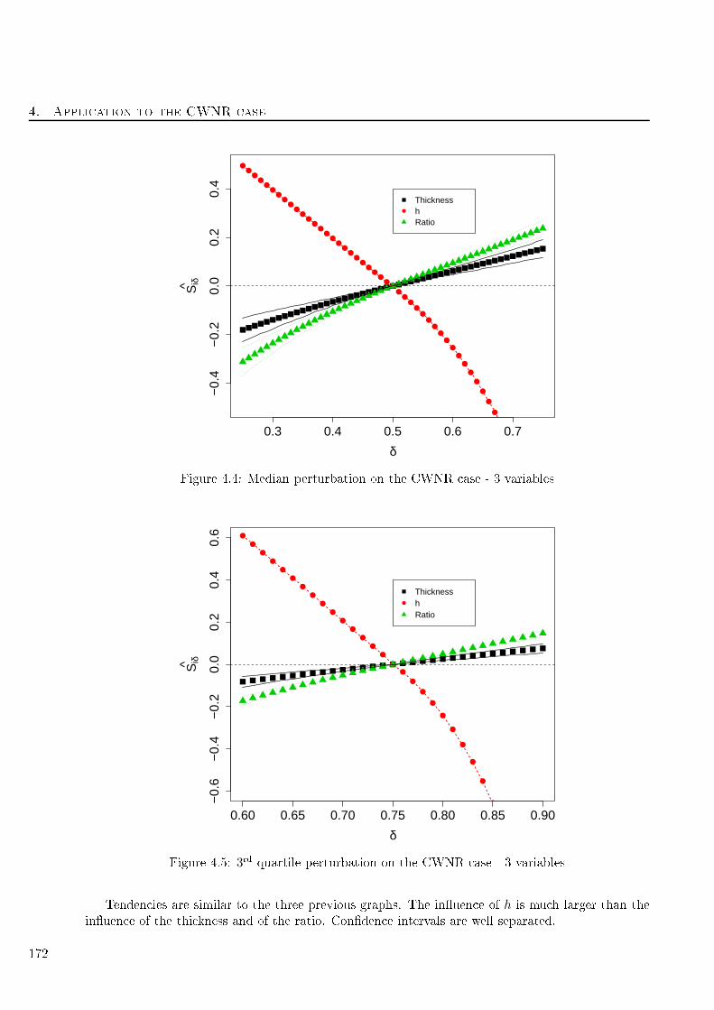
4. Appli ation to the CWNR ase
0.3 0.4 0.5 0.6 0.7
−0.
4−
0.2
0.0
0.2
0.4
δ
Siδ^
ThicknesshRatio
Figure 4.4: Median perturbation on the CWNR ase - 3 variables
0.60 0.65 0.70 0.75 0.80 0.85 0.90
−0.
6−
0.4
−0.
20.
00.
20.
40.
6
δ
Siδ^
ThicknesshRatio
Figure 4.5: 3rd quartile perturbation on the CWNR ase - 3 variables
Tenden ies are similar to the three previous graphs. The inuen e of h is mu h larger than the
inuen e of the thi kness and of the ratio. Conden e intervals are well separated.
172
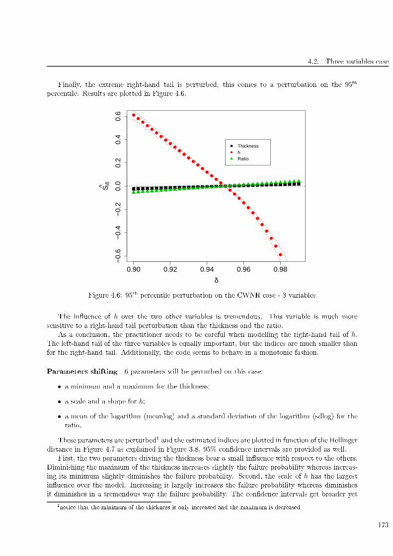
4.2. Three variables ase
Finally, the extreme right-hand tail is perturbed, this omes to a perturbation on the 95th
per entile. Results are plotted in Figure 4.6.
0.90 0.92 0.94 0.96 0.98
−0.
6−
0.4
−0.
20.
00.
20.
40.
6
δ
Siδ^
ThicknesshRatio
Figure 4.6: 95th per entile perturbation on the CWNR ase - 3 variables
The inuen e of h over the two other variables is tremendous. This variable is mu h more
sensitive to a right-hand tail perturbation than the thi kness and the ratio.
As a on lusion, the pra titioner needs to be areful when modelling the right-hand tail of h.The left-hand tail of the three variables is equally important, but the indi es are mu h smaller than
for the right-hand tail. Additionally, the ode seems to behave in a monotoni fashion.
Parameters shifting 6 parameters will be perturbed on this ase:
a minimum and a maximum for the thi kness;
a s ale and a shape for h;
a mean of the logarithm (meanlog) and a standard deviation of the logarithm (sdlog) for the
ratio.
These parameters are perturbed
1
and the estimated indi es are plotted in fun tion of the Hellinger
distan e in Figure 4.7 as explained in Figure 3.8. 95% onden e intervals are provided as well.
First, the two parameters driving the thi kness bear a small inuen e with respe t to the others.
Diminishing the maximum of the thi kness in reases slightly the failure probability whereas in reas-
ing its minimum slightly diminishes the failure probability. Se ond, the s ale of h has the largest
inuen e over the model. In reasing it largely in reases the failure probability whereas diminishes
it diminishes in a tremendous way the failure probability. The onden e intervals get broader yet
1
noti e that the minimum of the thi kness is only in reased and the maximum is de reased
173
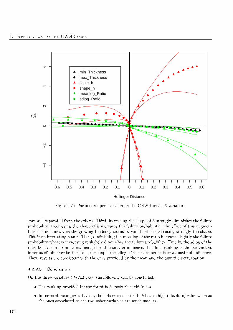
4. Appli ation to the CWNR ase
−4
−2
02
46
Hellinger Distance
Siδ^
0.6 0.5 0.4 0.3 0.2 0.1 0 0.1 0.2 0.3 0.4 0.5 0.6
min_Thicknessmax_Thicknessscale_hshape_hmeanlog_Ratiosdlog_Ratio
Figure 4.7: Parameters perturbation on the CNWR ase - 3 variables
stay well separated from the others. Third, in reasing the shape of h strongly diminishes the failure
probability. De reasing the shape of h in reases the failure probability. The ee t of this augmen-
tation is not linear, as the growing tenden y seems to vanish when de reasing strongly the shape.
This is an interesting result. Then, diminishing the meanlog of the ratio in reases slightly the failure
probability whereas in reasing it slightly diminishes the failure probability. Finally, the sdlog of the
ratio behaves in a similar manner, yet with a smaller inuen e. The nal ranking of the parameters
in terms of inuen e is: the s ale, the shape, the sdlog. Other parameters bear a quasi-null inuen e.
These results are onsistent with the ones provided by the mean and the quantile perturbation.
4.2.2.3 Con lusion
On the three variables CWNR ase, the following an be on luded:
The ranking provided by the forest is h, ratio then thi kness.
In terms of mean perturbation, the indi es asso iated to h have a high (absolute) value whereas
the ones asso iated to the two other variables are mu h smaller.
174
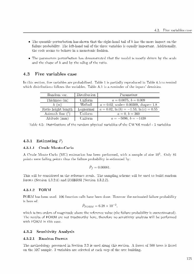
4.3. Five variables ase
The quantile perturbation has shown that the right-hand tail of h has the more impa t on the
failure probability. The left-hand tail of the three variables is equally important. Additionally,
the ode seems to behave in a monotoni fashion.
The parameters perturbation has demonstrated that the model is mostly driven by the s ale
and the shape of h and by the sdlog of the ratio.
4.3 Five variables ase
In this se tion, ve variables are probabilised. Table 1 is partially reprodu ed in Table 4.5 to remind
whi h distributions follows the variables. Table A.1 is a reminder of the inputs' densities.
Random var. Distribution Parameters
Thi kness (m) Uniform a = 0.0075, b = 0.009
h (m) Weibull a = 0.02, s ale= 0.00309, shape= 1.8
Ratio height/length Lognormal a = 0.02, ln (b) = −1.53, ln (c) = 0.55
Azimuth aw (°) Uniform a = 0, b = 360
Altitude (mm) Uniform a = −5096, b = −1438
Table 4.5: Distributions of the random physi al variables of the CWNR model - 5 variables
4.3.1 Estimating Pf
4.3.1.1 Crude Monte-Carlo
A Crude Monte-Carlo (MC) estimation has been performed, with a sample of size 105. Only 81points were failing points thus the failure probability is estimated by:
Pf = 0.00081.
This will be onsidered as the referen e result. The sampling s heme will be used to build random
forests (Se tion 4.3.2.1) and DMBRSI (Se tion 4.3.2.2).
4.3.1.2 FORM
FORM has been used. 106 fun tion alls have been done. However the estimated failure probability
is here of:
PFORM = 6.28 × 10⁻²,
whi h is two orders of magnitude above the referen e value (the failure probability is overestimated).
The results of FORM are not trustworthy here, therefore no sensitivity analysis will be performed
with FORM in this ase.
4.3.2 Sensitivity Analysis
4.3.2.1 Random Forests
The methodology presented in Se tion 2.2 is used along this se tion. A forest of 500 trees is tted
on the MC sample. 2 variables are sele ted at ea h step of the tree building.
175
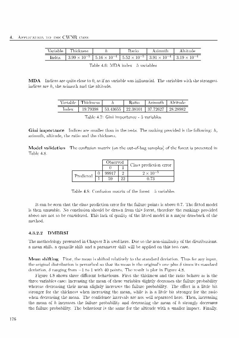
4. Appli ation to the CWNR ase
Variable Thi kness h Ratio Azimuth Altitude
Index 3.99 × 10⁻⁵ 5.16 × 10⁻⁴ 5.52 × 10⁻⁵ 3.91× 10⁻⁴ 3.19× 10⁻⁴
Table 4.6: MDA index - 5 variables
MDA Indi es are quite lose to 0, as if no variable was inuential. The variables with the strongestindi es are h, the azimuth and the altitude.
Variable Thi kness h Ratio Azimuth Altitude
Index 19.79398 53.43655 22.38101 37.72627 28.28982
Table 4.7: Gini importan e - 5 variables
Gini importan e Indi es are smaller than in the tests. The ranking provided is the following: h,azimuth, altitude, the ratio and the thi kness.
Model validation The onfusion matrix (on the out-of-bag samples) of the forest is presented in
Table 4.8.
Observed
Class predi tion error
0 1
Predi ted
0 99917 2 2× 10⁻⁵
1 59 22 0.73
Table 4.8: Confusion matrix of the forest - 5 variables
It an be seen that the lass predi tion error for the failure points is above 0.7. The tted model
is then unusable. No on lusion should be drawn from this forest, therefore the rankings provided
above are not to be onsidered. This la k of quality of the tted model is a major drawba k of the
method.
4.3.2.2 DMBRSI
The methodology presented in Chapter 3 is used here. Due to the non-similarity of the distributions,
a mean shift, a quantile shift and a parameter shift will be applied on this test ase.
Mean shifting First, the mean is shifted relatively to the standard deviation. Thus for any input,
the original distribution is perturbed so that its mean is the original's one plus δ times its standard
deviation, δ ranging from −1 to 1 with 40 points. The result is plot in Figure 4.8.
Figure 4.8 shows three dierent behaviours. First the thi kness and the ratio behave as is the
three variables ase: in reasing the mean of these variables slightly de reases the failure probability
whereas de reasing their mean slightly in reases the failure probability. The ee t is a little bit
stronger for the thi kness when in reasing the mean, while it is a little bit stronger for the ratio
when de reasing the mean. The onden e intervals are not well separated here. Then, in reasing
the mean of h in reases the failure probability and de reasing the mean of h strongly de reases
the failure probability. The behaviour is the same for the altitude with a smaller impa t. Finally,
176

4.3. Five variables ase
−1.0 −0.5 0.0 0.5 1.0
−4
−2
02
4
δ
Siδ^
ThicknesshRatioAzimuthAltitude
Figure 4.8: Estimated indi es Siδ for the CWNR ase with a mean perturbation - 5 variables
in reasing or de reasing the mean of the azimuth slightly in reases the failure probability. The two
more inuential variables here are h and the altitude, yet it has to be noti ed that h is of primary
importan e.
Quantile shifting The rst quantile to be perturbed is the extreme left-hand tail, namely the
5%-quantile. The result of su h a perturbation for all the variables is plotted in Figure 4.9.
This graph shows two opposite behaviours. First, de reasing the weight of the 5th per entile
de reases the failure probability for the thi kness, the ratio and the azimuth. For these variables,
in reasing the weight of the onsidered quantile in reases the failure probability. Then, the behaviour
is reversed for h and the altitude. Con erning the variable ranking, the azimuth has the more
inuen e, while the altitude and h have the same small inuen e. The ratio has a larger inuen e
than the thi kness, but the onden e intervals are not well separated here.
The 1st quartile is then perturbed and the results are plotted in Figure 4.10.
When perturbing less extreme values of the left-hand tail, the behaviour are similar, but the
order of inuen e is modied. In parti ular, the azimuth that was the most inuential variable in
Figure 4.9 is now the less inuential. Then omes the thi kness, and the three remaining variables
have an equivalent inuen e.
The median of the input distributions is then perturbed, the resulting indi es are plotted in
Figure 4.11.
When perturbing the median, tenden ies are similar to the two previous graphs for the thi kness,
h, the ratio and the altitude. However, the tenden y is modied for the azimuth: in reasing the
weight of the median slightly de reases the failure probability whereas de reasing the weight in reases
177
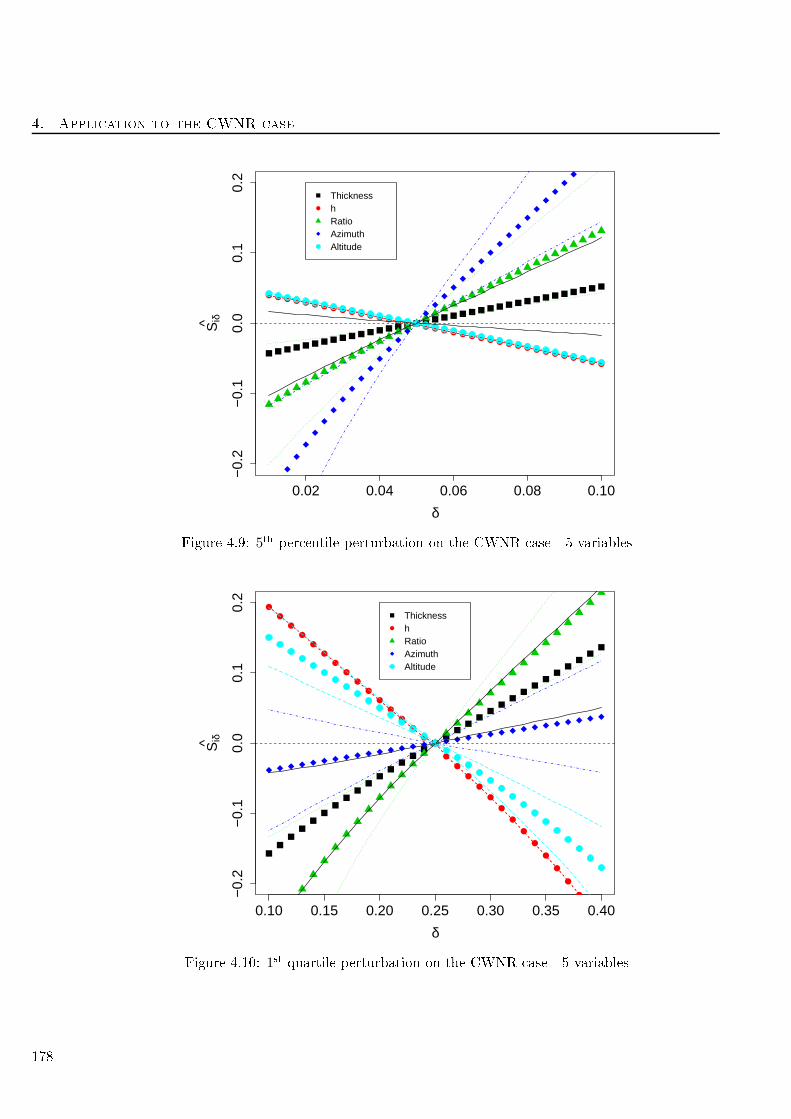
4. Appli ation to the CWNR ase
0.02 0.04 0.06 0.08 0.10
−0.
2−
0.1
0.0
0.1
0.2
δ
Siδ^
ThicknesshRatioAzimuthAltitude
Figure 4.9: 5th per entile perturbation on the CWNR ase - 5 variables
0.10 0.15 0.20 0.25 0.30 0.35 0.40
−0.
2−
0.1
0.0
0.1
0.2
δ
Siδ^
ThicknesshRatioAzimuthAltitude
Figure 4.10: 1st quartile perturbation on the CWNR ase - 5 variables
178

4.3. Five variables ase
0.3 0.4 0.5 0.6 0.7
−0.
6−
0.4
−0.
20.
00.
20.
4
δ
Siδ^
ThicknesshRatioAzimuthAltitude
Figure 4.11: Median perturbation on the CWNR ase- 5 variables
the failure probability. The inuen e of h is the largest, then omes the altitude, followed by the
ratio and the thi kness. The azimuth has the smallest inuen e.
The third quartile is then perturbed and the indi es are plotted in Figure 4.12.
Tenden ies are similar to the previous graphs. The inuen e of h and of the altitude is larger
than the one of the other variables. Conden e intervals are well separated ex ept for the ratio and
the thi kness.
Finally, the extreme right-hand tail is perturbed, this omes to a perturbation on the 95th
per entile. Results are plotted in Figure 4.13.
179

4. Appli ation to the CWNR ase
0.60 0.65 0.70 0.75 0.80 0.85 0.90
−1.
0−
0.5
0.0
0.5
δ
Siδ^
ThicknesshRatioAzimuthAltitude
Figure 4.12: 3rd quartile perturbation on the CWNR ase - 5 variables
0.90 0.92 0.94 0.96 0.98
−1.
0−
0.5
0.0
0.5
1.0
δ
Siδ^
ThicknesshRatioAzimuthAltitude
Figure 4.13: 95th per entile perturbation on the CWNR ase - 5 variables
The inuen e of h over the other variables is tremendous. The azimuth is also more inuential
180

4.3. Five variables ase
than the three remaining variables.
As a on lusion, the pra titioner needs to be areful when modelling the right-hand tail of h,and the tails of the azimuth. In terms of value of the indi es, the right-hand tails have mu h more
impa t than the left-hand tails. Additionally, this analysis revealed the non-monotoni behaviour of
the azimuth.
Parameters shifting 10 parameters will be perturbed on this ase:
a minimum and a maximum for the thi kness;
a s ale and a shape for h;
a mean of the logarithm (meanlog) and a standard deviation of the logarithm (sdlog) for the
ratio.
a minimum and a maximum for the azimuth;
a minimum and a maximum for the altitude;
These parameters are perturbed so that the support is not in reased: the minimums are only
in reased and the maximums are de reased. The estimated indi es are plotted in fun tion of the
Hellinger distan e in Figure 4.14 as explained in Figure 3.8. 95% onden e intervals are provided
as well.
Due to the large number of parameters perturbed, the image is di ult to read. However, the
inuen e of the parameters driving h (plotted in red) is tremendous. The indi es asso iated to the
s ale are larger than the ones asso iated to the shape, however the width of the onden e intervals
grows quite large, thus it is di ult to on lude on these two parameters. Then, the maximum of
the altitude seems to have the most inuen e over the failure probability. Diminishing the maximum
of the altitude leads to a de rease of the failure probability. It is followed by the meanlog of the
ratio. The indi es asso iated with other parameters are too noisy and sta ked around 0.
4.3.2.3 Con lusion
On the ve variables CWNR ase, the following an be on luded:
The ranking provided by the forest is not to be onsidered as the model is badly tted.
In terms of mean perturbation, the indi es asso iated to h have the highest (absolute) value.
Then omes the altitude, followed by the ratio, the azimuth and the thi kness. Noti e that
the relative inuen e of the ratio, the azimuth and the thi kness is hardly separable.
The quantile perturbation has shown that the right-hand tail of h, and the tails of the azimuth
are more inuential than the tails of others variable. The right-hand tails have mu h more
impa t than the left-hand tails though. Additionally, this analysis revealed the non-monotoni
behaviour of the azimuth.
The parameters perturbation has demonstrated that the model is mostly driven by the s ale
and the shape of h. Then, the maximum of the altitude seems to have the most inuen e over
the failure probability, followed by the meanlog of the ratio.
It is noti eable that the ranking diers from the three variables ase, yet the dimension of the
aw h is still the most inuential variable. Additionally, it seems interesting to noti e that the
altitude is inuential, but mostly in the right-hand tail (see Figure 4.12).
181

4. Appli ation to the CWNR ase
−20
−10
010
20
Hellinger Distance
Siδ^
0.6 0.5 0.4 0.3 0.2 0.1 0 0.1 0.2 0.3 0.4 0.5 0.6
min_Thicknessmax_Thicknessscale_hshape_hmeanlog_Ratiosdlog_Ratiomin_Azimuthmax_Azimuthmin_Altitudemax_Altitude
Figure 4.14: Parameters perturbation on the CNWR ase - 5 variables
4.4 Seven variables ase
In this se tion, seven variables are probabilised. Table 1 is reprodu ed in Table 4.9 to remind whi h
distributions follows the variables. Table A.1 is a reminder of the inputs' densities.
Random var. Distribution Parameters
Thi kness (m) Uniform a = 0.0075, b = 0.009
h (m) Weibull a = 0.02, s ale= 0.00309, shape= 1.8
Ratio height/length Lognormal a = 0.02, ln (b) = −1.53, ln (c) = 0.55
Azimuth aw (°) Uniform a = 0, b = 360
Altitude (mm) Uniform a = −5096, b = −1438
σ∆TT Gaussian µ = 0, σ = 1
σRes Gaussian µ = 0, σ = 1
Table 4.9: Distributions of the random physi al variables of the CWNR model - 7 variables
182

4.4. Seven variables ase
4.4.1 Estimating Pf
4.4.1.1 Crude Monte-Carlo
A Crude Monte-Carlo (MC) estimation has been performed, with a sample of size 7 × 10⁶. Noti ethat this samples took several weeks to be omputed. 468 points were failing points thus the failure
probability is estimated by:
Pf = 6.68 × 10⁻⁵.
This will be onsidered as the referen e result.
4.4.1.2 FORM
FORM has been used. 183 fun tion alls have been done. The estimated failure probability is here
of:
PFORM = 4.23 × 10⁻⁷,
whi h is two orders of magnitude under the referen e value (the failure probability is underestimated).
The results of FORM are not trustworthy in this ase.
4.4.2 Sensitivity Analysis
4.4.2.1 Random Forests
The methodology presented in Se tion 2.2 is used along this se tion. We tried to t a forest of 500trees on the MC sample whi h dimension was 7× 7000000, with 2 variables sele ted at ea h step of
the tree building. However the tting step failed due to the size of the sample (as in Se tion 2.2.5.2,
paragraph "in reasing the sample size").
4.4.2.2 DMBRSI
The methodology presented in Chapter 3 is used here. Due to the non-similarity of the distributions,
a mean shift, a quantile shift and a parameter shift will be applied on this test ase.
Mean shifting First, the mean is shifted relatively to the standard deviation. Thus for any input,
the original distribution is perturbed so that its mean is the original's one plus δ times its standard
deviation, δ ranging from −1 to 1 with 40 points. The result is plot in Figure 4.15.
Three dierent behaviours an be observed. When in reasing the mean of h, of the altitude
and of σ∆TT it in reases the failure probability while when de reasing their means it de reases the
failure probability. The ee t is reversed for the thi kness, the ratio and σRes. Finally, in reasing orde reasing the mean of the azimuth slightly in reases the failure probability. In terms of amplitude,
three variables dierentiate themselves from the others: h, σ∆TT and σRes. Others variables havea smaller inuen e and their onden e intervals ontains 0.
Quantile shifting The rst quantile to be perturbed is the extreme left-hand tail, namely the
5%-quantile. The result of su h a perturbation for all the variables is plotted in Figure 4.16.
It rst should be noti es that the indi es for h and for σ∆TT oin ide. This graph shows
two opposite behaviours. First, de reasing the weight of the 5th per entile de reases the failure
probability for the thi kness, the ratio, the azimuth and for σRes. For these variables, in reasing
the weight of the onsidered quantile in reases the failure probability. Then, the behaviour is reversed
for h, the altitude and σ∆TT . Con erning the variable ranking, σRes has the more inuen e. Then
183

4. Appli ation to the CWNR ase
−1.0 −0.5 0.0 0.5 1.0
−1.0
−0.5
0.0
0.5
1.0
1.5
2.0
δ
δ
σ∆
σ
Figure 4.15: Estimated indi es Siδ for the CWNR ase with a mean perturbation - 7 variables
omes the azimuth that has a medium inuen e, while the rest of the variables have the same small
inuen e.
The 1st quartile is then perturbed and the results are plotted in Figure 4.17.
The indi es for h and for the altitude oin ide. When perturbing less extreme values of the left-
hand tail, the behaviour are similar, but the order of inuen e is modied. The azimuth that was
an inuential variable in Figure 4.16 is now the less inuential. The two most inuential variables
are σ∆TT and σRes.
The median of the input distributions is then perturbed, the resulting indi es are plotted in
Figure 4.18.
When perturbing the median, tenden ies are similar to the two previous graphs for all the
variables but the azimuth. Indeed in reasing or de reasing the weight of the median for this variable
does not impa t the failure probability. The inuen e of σ∆TT is the largest, followed by h and
σRes that have a similar impa t (but a dierent behaviour). Then omes the ratio and the thi kness.
The two other variables have a small to null impa t.
The third quartile is then perturbed and the indi es are plotted in Figure 4.19.
Tenden ies are similar to the previous graphs ex ept for the altitude and the thi kness. The
inuen e of h and of σ∆TT is larger than the one of the other variables. The impa t of the ratio
and of σRes is similar.
Finally, the extreme right-hand tail is perturbed, this omes to a perturbation on the 95th
per entile. Results are plotted in Figure 4.20.
This gure shows learly the impa t of the following variables (for whi h in reasing the weight
of the quantile de reases the failure probability), ordered by inuen e: h, σ∆TT , the azimuth. Theothers variables have a small to null impa t.
184
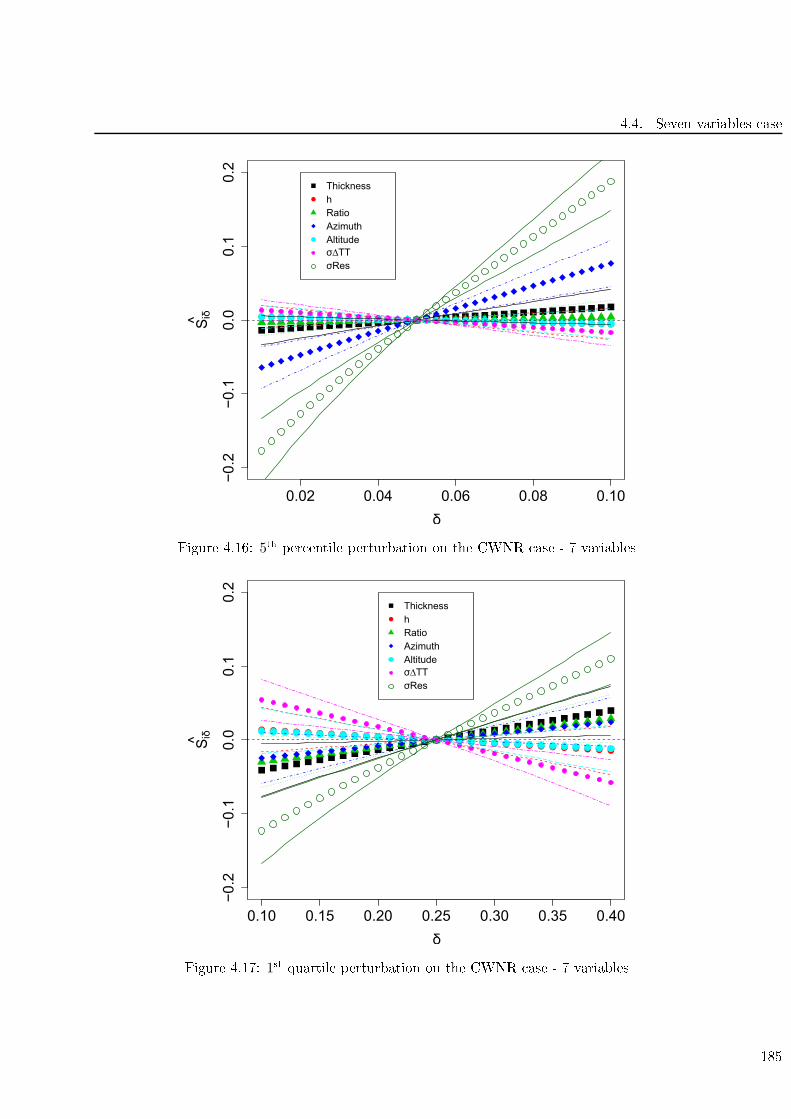
4.4. Seven variables ase
0.02 0.04 0.06 0.08 0.10
−0.2
−0.1
0.0
0.1
0.2
δ
Siδ^
Thickness
h
Ratio
Azimuth
Altitude
σ∆TT
σRes
Figure 4.16: 5th per entile perturbation on the CWNR ase - 7 variables
0.10 0.15 0.20 0.25 0.30 0.35 0.40
−0.2
−0.1
0.0
0.1
0.2
δ
Siδ^
Thickness
h
Ratio
Azimuth
Altitude
σ∆TT
σRes
Figure 4.17: 1st quartile perturbation on the CWNR ase - 7 variables
185

4. Appli ation to the CWNR ase
0.3 0.4 0.5 0.6 0.7
−0.2
0.0
0.2
0.4
δ
Siδ^
Thickness
h
Ratio
Azimuth
Altitude
σ∆TT
σRes
Figure 4.18: Median perturbation on the CWNR ase- 7 variables
0.60 0.65 0.70 0.75 0.80 0.85 0.90
0.3
0.2
0.1
0.0
0.1
0.2
0.3
Si^
Thickness
h
Ratio
Azimuth
Altitude
σ∆TT
σRes
Figure 4.19: 3rd quartile perturbation on the CWNR ase - 7 variables
186
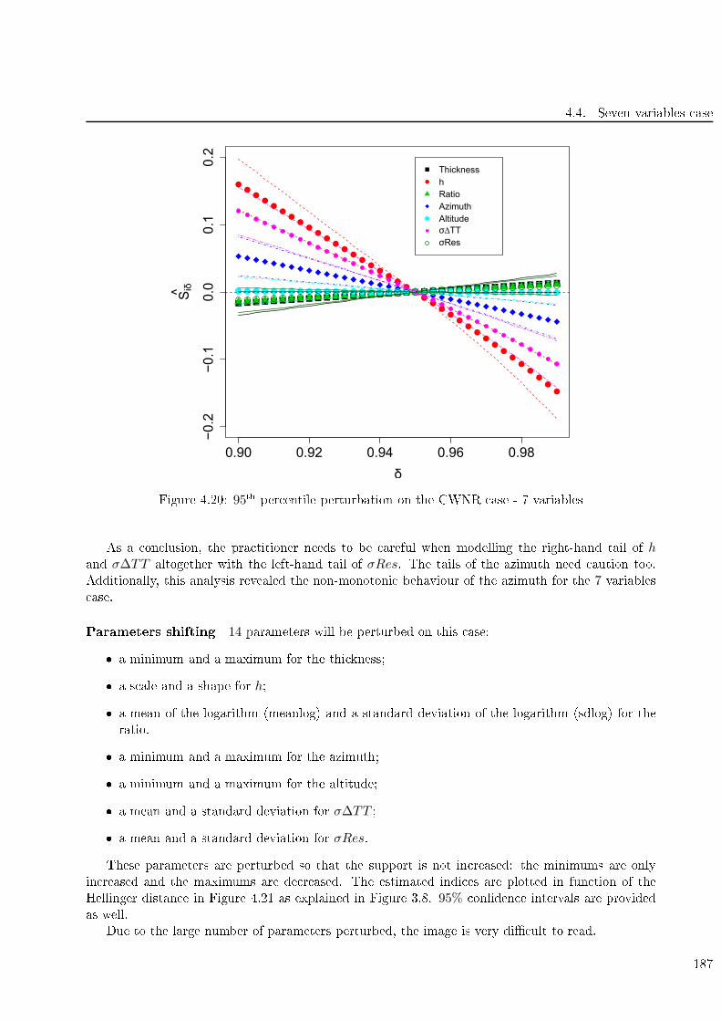
4.4. Seven variables ase
0.90 0.92 0.94 0.96 0.98
−0.2
−0.1
0.0
0.1
0.2
δ
Siδ^
Thickness
h
Ratio
Azimuth
Altitude
σ∆TT
σRes
Figure 4.20: 95th per entile perturbation on the CWNR ase - 7 variables
As a on lusion, the pra titioner needs to be areful when modelling the right-hand tail of hand σ∆TT altogether with the left-hand tail of σRes. The tails of the azimuth need aution too.
Additionally, this analysis revealed the non-monotoni behaviour of the azimuth for the 7 variables
ase.
Parameters shifting 14 parameters will be perturbed on this ase:
a minimum and a maximum for the thi kness;
a s ale and a shape for h;
a mean of the logarithm (meanlog) and a standard deviation of the logarithm (sdlog) for the
ratio.
a minimum and a maximum for the azimuth;
a minimum and a maximum for the altitude;
a mean and a standard deviation for σ∆TT ;
a mean and a standard deviation for σRes.
These parameters are perturbed so that the support is not in reased: the minimums are only
in reased and the maximums are de reased. The estimated indi es are plotted in fun tion of the
Hellinger distan e in Figure 4.21 as explained in Figure 3.8. 95% onden e intervals are provided
as well.
Due to the large number of parameters perturbed, the image is very di ult to read.
187
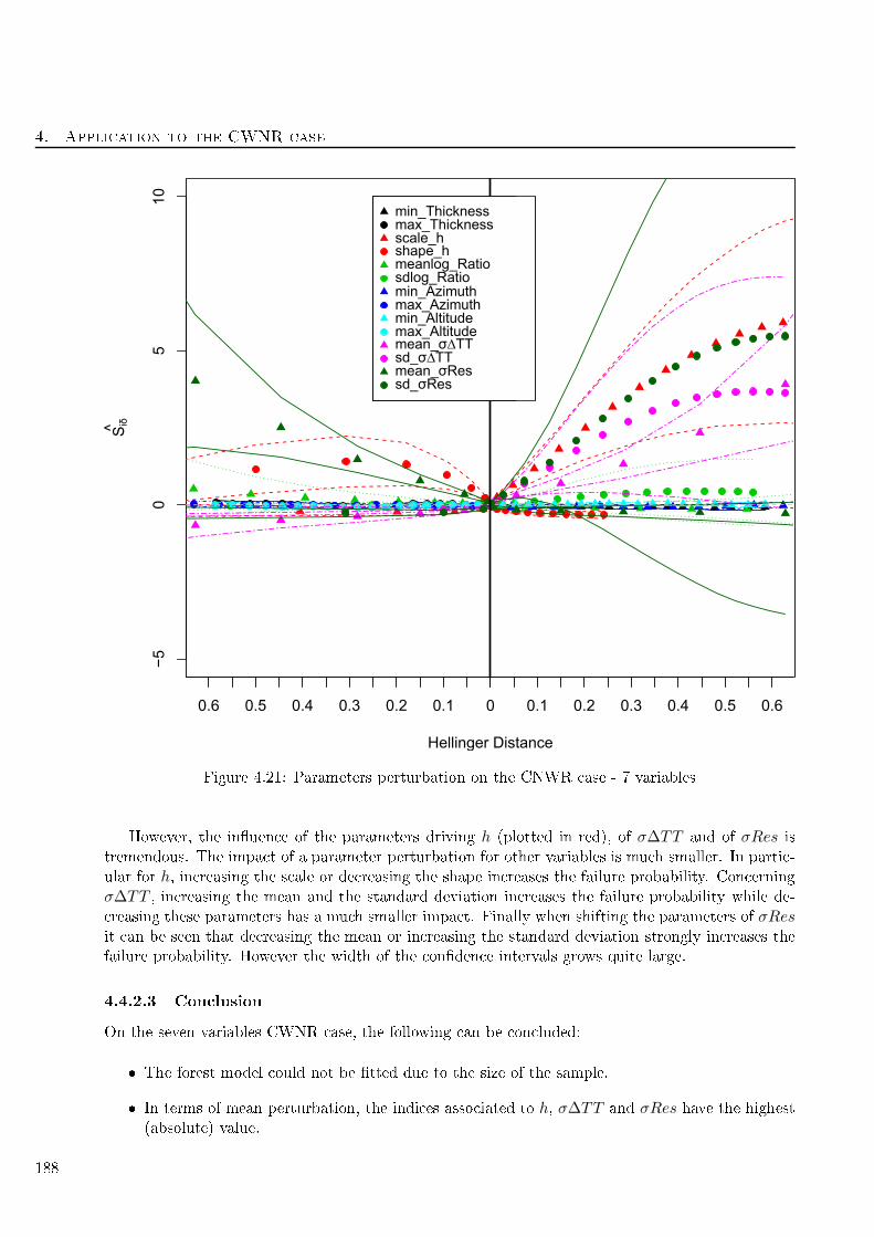
4. Appli ation to the CWNR ase
−5
05
10
Hellinger Distance
Siδ^
0.6 0.5 0.4 0.3 0.2 0.1 0 0.1 0.2 0.3 0.4 0.5 0.6
min_Thicknessmax_Thicknessscale_hshape_hmeanlog_Ratiosdlog_Ratiomin_Azimuthmax_Azimuthmin_Altitudemax_Altitudemean_sigma RTNDTsd_sigma RTNDTmean_sigmaK1Csd_sigmaK1C
min_Thicknessmax_Thicknessscale_hshape_hmeanlog_Ratiosdlog_Ratiomin_Azimuthmax_Azimuthmin_Altitudemax_Altitudemean_σ∆TTsd_σ∆TTmean_σRessd_σRes
Figure 4.21: Parameters perturbation on the CNWR ase - 7 variables
However, the inuen e of the parameters driving h (plotted in red), of σ∆TT and of σRes is
tremendous. The impa t of a parameter perturbation for other variables is mu h smaller. In parti -
ular for h, in reasing the s ale or de reasing the shape in reases the failure probability. Con erning
σ∆TT , in reasing the mean and the standard deviation in reases the failure probability while de-
reasing these parameters has a mu h smaller impa t. Finally when shifting the parameters of σResit an be seen that de reasing the mean or in reasing the standard deviation strongly in reases the
failure probability. However the width of the onden e intervals grows quite large.
4.4.2.3 Con lusion
On the seven variables CWNR ase, the following an be on luded:
The forest model ould not be tted due to the size of the sample.
In terms of mean perturbation, the indi es asso iated to h, σ∆TT and σRes have the highest(absolute) value.
188
4.5. Con lusion
The quantile perturbation has shown that the right-hand tail of h and σ∆TT altogether with
the left-hand tail of σRes and the tails of the azimuth are more inuential than the tails
of others variable. Additionally, this analysis revealed the non-monotoni behaviour of the
azimuth.
The parameters perturbation has demonstrated that the model is mostly driven by the pa-
rameters of h of σ∆TT and of σRes . This onrms the on lusion of the mean perturbation.
It is noti eable that the ranking diers from the three and the ve variables ase. However the
dimension of the aw h is still an inuential variable.
4.5 Con lusion
Con erning the Pf estimation part, the MC method is still the referen e method on an industrial
ode. The major drawba k is of ourse the omputational time needed. FORM is wrong in all the
ases and should not be used.
Con erning the sensitivity analysis part, the random forest te hnique provides questionable re-
sults, sin e the tted models are uneven or bad. This method is in on lusive at the moment.
DMBRSI seems an adapted method to perform sensitivity analysis on a failure event. Several
tunings for several problems have been tested. However, if a single graph had to be provided to
de ision makers, we would present the mean perturbation one, as it arries most of the information.
In all the onguration studied, h is a priority variable. This is also the ase for σ∆TT and
σRes in the 7 variables ase.
The improvement perspe tives of this study are:
to ombine subset simulation with the DMBRSI. To do so, an implementation of subset sim-
ulation that provides the sampling s heme must be performed;
to ombine importan e sampling with the DMBRSI, now that the priority zones are known.
189


Con lusion
Summary and ontributions
This thesis' rst obje tive was to perform a sensitivity analysis on a bla k-box model, the CWNR
ase. Be ause the quantity of interest is a (small) failure probability, appropriate methods had to
be used. Thus this thesis fo used on two elds: stru tural reliability in one hand, and sensitivity
analysis on the other hand.
First step was a bibliographi al hapter (Chapter 1). This hapter aimed at larifying the main
existing te hniques to estimate a failure probability (Se tion 1.2) and the main sensitivity analysis
methods (Se tion 1.3). Then one of the most used sensitivity analysis te hnique (Sobol' indi es)
was tested on reliability toy- ases (Se tion 1.4). Sobol' indi es applied to a failure indi ator have
highlighted a apa ity to distinguish the non-inuential from the inuential variables. However, tests
have shown that the following onguration -low rst-order indi es, high total order indi es- is often
present. Therefore the information provided by su h indi es is limited and may only onrm that all
the variables intera t to ause the failure event. Next, a moment-independent method (Borgonovo's
δi indi es) was tested on reliability toy- ases (Se tion 1.5). However, the produ ed indi es were
rather small with a positive bias in the estimations. The on lusion is that moment independent
te hniques are not adapted within the reliability ontext. A synthesis of the tested methods was
proposed in Se tion 1.6. Finally, a dis ussion on the meaning and obje tives of sensitivity analysis
when dealing with failure probabilities, that we argue might be of use for the pra titioner, was
ondu ted in Se tion 1.7.
The on lusion of this bibliographi al hapter is that there is a need for new sensitivity analysis
methods in the reliability ontext. The next two hapters aimed at rea hing this obje tive.
The se ond hapter fo used on sensitivity analysis te hniques with a variable ranking obje tive.
Two sensitivity analysis methods were presented, thought as by-produ ts of two sampling te hniques
(Monte-Carlo and subset simulation). The rst part of the hapter (Se tion 2.2) was devoted to
importan e measures derived from random forests.
Reminders on spe i binary lassiers (random trees) were proposed altogether with a review
on stabilisation methods, in luding random forests. The importan e measures (Gini importan e and
Mean De rease A ura y importan e) were eli ited. Then a bibliographi al step was performed on
the "sensitivity analysis using random forests" theme. Then the importan e measures have been
tested on reliability toy- ases. The on lusions were that the Mean De rease A ura y importan e
indi es seemed more adapted sin e the Gini importan e indi es ould ae t a non-null importan e
to a non-inuential variable. However, it must be stressed that the tted models' quality is not
satisfying. Indeed, from the imbalan e of the lasses in the original sample, there is a tenden y in
getting "weak" predi tors that make mu h more predi tion error on the minority lass. This is a
problem when drawing on lusions on sensitivity analysis with these types of models. The se ond
191

Con lusion
part of the hapter (Se tion 2.3) proposed a new sensitivity measure based upon the departure, at
ea h step of a subset method, between ea h input original density and the density given the subset
rea hed. Several tunings of the departure an be used. However this sensitivity analysis method
gives a similar information that the one provided by the Sobol' indi es on the failure indi ator.
The third hapter presented an original sensitivity analysis method, alled Density Modi ation
Based Reliability Sensitivity Indi es (DMBRSI). This sensitivity index is based upon input density
modi ation, and is adapted to failure probabilities. The proposed indi es ree t the impa t of
an input density modi ation on the failure probability. One needs to dierentiate the proposed
index and the perturbations. The indi es are independent of the perturbation in the sense that
the pra titioner an set the perturbation adapted to his/her problem. The sensitivity index an
be omputed using the sole set of simulations that has already been used to estimate the failure
probability, thus limiting the number of alls to the numeri al model.
First, the indi es and their theoreti al properties have been presented in Se tion 3.2, altogether
with the estimation methodology. For the sake of simpli ity, a Monte-Carlo sampling s heme was
onsidered. Se ond, Se tion 3.3 dealt with several perturbation methodologies. These perturbations
an be lassied into two main families: Kullba k-Leibler minimization methods and parameter
perturbations methods. The behaviour of the indi es was examined in Se tion 3.4 through numeri al
simulations. In Se tion 3.5, it was proposed to improve the DMBRSI estimation with importan e
sampling and with subset simulation.
This hapter presented an original method designed for failure probabilities. One of the main
advantage is the possibility to modify the perturbation applied without new alls to the model.
However a major drawba k persists: when there are too many parameters to perturb, the results
may be ompli ated to interpret.
The fourth hapter presented the appli ation of some of the developed methods to the CWNR
ase. Remind that this bla k-box model provided the initial motivation for this thesis.
To estimate Pf , two methods were used: rude Monte-Carlo and FORM. It appeared that FORM
was wrong in every ase, thus Monte-Carlo stays the referen e method.
The sensitivity analysis part then fo used on two methods: random forests (Chapter 2), and
DMBRSI (Chapter 3). Sobol' indi es (see Se tion 1.4) were not tested in this hapter due to the
limited information provided and their high omputational ost. δSSi (Ak) indi es (see Se tion 2.3)
were not used either sin e a sampling s heme from subset simulation was not available.
This hapter is divided in three main se tions, fo using respe tively on random input of dimension
3 , dimension 5 and dimension 7. Noti e that the smaller the dimension of the input, the more
penalizing the ase (sin e non-probabilised variables are set to penalizing values). Thus the failure
probability diminishes as the dimensionality growths.
DMBRSI appeared as an adapted method to perform sensitivity analysis on a failure event. In
all the ongurations studied, h (the dimension of the aw) is a priority variable. This is also the
ase for σ∆TT and σRes in the 7 variables ase.
Future avenues for resear h and appli ation
The methods presented in Chapter 2 an be improved. Spe i ally, there is a need to improve the
binary lassiers (random forests). The MDA indi es when using subset simulation must be imple-
mented Another perspe tive of improvement, when using the δSSi (Ak) indi es, is to ondu t a work
192
in luding the opula theory.
The DMBRSI introdu ed in Chapter 3 have several ways of improvement. Most of the further
work will be devoted to adapting the estimator of the indi es Siδ in terms of varian e redu tion and
of number of fun tion alls. The adaptation of estimators using subset simulation must also be done.
A perturbation based on an entropy onstraint might also be proposed. Yet further omputations
have to be made to obtain a tra table solution of the KL minimization problem. Another avenue
worth exploring would be to hange the metri s/divergen es. That would amount to hange the
D in equation 3.9 ( hoi e was made to take KLD); and to take another distan e than Hellinger's
in the parameter perturbation ontext. Another avenue might be the introdu tion of a stru tural
dependen y between the marginals of the input ve tor, and to perturb this dependen y via the
opula theory.
Further work an be done in Chapter 4. The main improvement perspe tives of this study is
to use subset simulation, to improve the estimation of Pf and to redu e the omputational time.
A oupling with the random forests via adapted MDA indi es might be of interest as well. This
ould also allow the use of the .d.f. departure measures δSSi (Ak). Still to redu e the varian e of theestimators, importan e sampling must be tested.
Broader perspe tives have to be onsidered. In parti ular, the use of sequential methods oupled
with meta-models (Be t et al. [9) is to be tested.
Re ently, Fort et al. [35 introdu ed a new sensitivity index as a generalisation of Sobol' indi es.
They propose an adapted ontrast fun tion for ea h statisti al purpose. It is interesting to noti e
that the ontrast adapted to a threshold ex eed is presented. This index then has to be tested and
ompared with DMBRSI in further work.
193
Con lusion
Communi ations
Publi ations
P. Lemaître, E. Sergienko, A. Arnaud, N. Bousquet, F. Gamboa, and B. Iooss. Density modi-
ation based reliability sensitivity analysis. Journal of Statisti al Computation and Simulation,
In press, 2014
E. Sergienko, P. Lemaître, A. Arnaud, D. Busby and F. Gamboa. Reliability sensitivity analysis
based on probability distribution perturbation with appli ation to CO2 storage. A epted with
minor reviews in Stru tural Safety, 2014
Oral presentations
P. Lemaître and A. Arnaud. Hiérar hisation des sour es d'in ertitudes vis à vis d'une proba-
bilité de dépassement de seuil - Une méthode basée sur la pondération des lois. In Pro eedings
des 43 èmes Journées de Statistique, Tunis, Tunisia, June 2011.
P. Lemaître. Analyse de sensibilité pour des probabilités de dépassement de seuil. In Pro eed-
ings of GdR MASCOT NUM, Bruyères-le-Châtel, Fran e, Mar h 2012.
P. Lemaître, E. Sergienko, F. Gamboa and B. Iooss. A global sensitivity analysis method for
reliability based upon density modi ation. In Pro eedings of SIAM Conferen e on Un ertainty
Quanti ation, Raleigh, North Carolina USA, April 2012.
A.L. Popelin, A. Dutfoy and P. Lemaître. Open TURNS: Open sour e Treatment of Un er-
tainty, Risk 'N Statisti s. In Pro eedings of SIAM Conferen e on Un ertainty Quanti ation,
Raleigh, North Carolina USA, April 2012.
P. Lemaître, A. Arnaud and B. Iooss. Sensitivity analysis methods for a failure probability.
In Pro eedings of Lambda Mu 18, Tours, Fran e, O tober 2012.
Poster
P. Lemaître, E. Sergienko, A. Arnaud, N. Bousquet, F. Gamboa, and B. Iooss. Sensitivity
analysis method for failure probability. Poster presented at SAMO 2013, Ni e, Fran e, June
2013.
Software developments
P. Lemaître. Density modi ation based reliability sensitivity indi es (DMBRSI Fun tion). R
Sensitivity Pa kage: http:// ran.r-proje t.org/web/pa kages/sensitivity/
194
Bibliography
[1 T. Abdo and R. Ra kwitz. A new beta-point algorithm for large time-invariant and time-
variant reliability problems. Reliability and Optimization of Stru tural Systems, 90:111, 1990.
[2 G. Andrianov, S. Burriel, S. Cambier, A. Dutfoy, I. Dutka-Malen, E. De Ro quigny, B. Sudret,
P. Benjamin, R. Lebrun, F. Mangeant, et al. Open TURNS, an open sour e initiative to treat
un ertainties, risks' n statisti s in a stru tured industrial approa h. In ESREL'2007 safety
and reliability onferen e, Stavenger, Norway, 2007.
[3 K. J. Ar her and R. V. Kimes. Empiri al hara terization of random forest variable importan e
measures. Computational Statisti s & Data Analysis, 52(4):22492260, 2008.
[4 S.K. Au and J.L. Be k. Estimation of small failure probabilities in high dimensions by subset
simulation. Probabilisti Engineering Me hani s, 16(4):263277, 2001.
[5 B. Auder, A. De Cre y, B. Iooss, and M. Marques. S reening and metamodeling of om-
puter experiments with fun tional outputs. appli ation to thermalhydrauli omputations.
Reliability Engineering & System Safety, 107:122131, 2012.
[6 B. Auder and B. Iooss. Global sensitivity analysis based on entropy. In Safety, Reliability
and Risk Analysis - Pro eedings of the ESREL 2008 Conferen e, pages 21072115. CRC Press,
september 2008.
[7 M. Balesdent, J. Morio, and J. Marzat. Re ommendations for the tuning of rare event proba-
bility estimators. Sumbitted, 2011.
[8 R.J. Be kman and M.D M Kay. Monte-Carlo estimation under dierent distributions using
the same simulation. Te hnometri s, 29(2):153160, 1987.
[9 J. Be t, D. Ginsbourger, L. Li, V. Pi heny, and E. Vazquez. Sequential design of omputer
experiments for the estimation of a probability of failure. Statisti s and Computing, 22(3):121,
2011.
[10 P. Bernardara, E. de Ro quigny, N. Goutal, A. Arnaud, and G. Passoni. Un ertainty analysis
in ood hazard assessment: hydrologi al and hydrauli alibration. Canadian Journal of Civil
Engineering, 37(7):968979, 2010.
[11 P. Besse. Apprentissage statistique & data mining. Institut de Mathématiques de Toulouse,
Laboratoire de Statistique et Probabilités UMR CNRS C, 2008.
[12 G. Biau, L. Devroye, and G. Lugosi. Consisten y of random forests and other averaging
lassiers. The Journal of Ma hine Learning Resear h, 9:20152033, 2008.
195
Bibliography
[13 E. Borgonovo. A new un ertainty importan e measure. Reliability Engineering & System
Safety, 92(6):771784, 2007.
[14 E. Borgonovo, W. Castaings, and S. Tarantola. Moment independent importan e measures:
new results and analyti al test ases. Risk Analysis, 31(3):404428, 2011.
[15 L. Breiman. Bagging predi tors. Ma hine learning, 24(2):123140, 1996.
[16 L. Breiman. Random forests. Ma hine learning, 45(1):532, 2001.
[17 L. Breiman, J. Friedman, C. J. Stone, and R. A. Olshen. Classi ation and regression trees.
Chapman & Hall/CRC, 1984.
[18 K. Breitung. Asymptoti approximations for multinormal integrals. Journal of Engineering
Me hani s, 110:357, 1984.
[19 B. Briand. Constru tion d
′arbres de dis rimination pour expliquer les niveaux de ontamination
radioa tive des végétaux. PhD thesis, Université Montpellier II, Fran e, 2008.
[20 B. Briand, G. R. Du harme, V. Para he, and C. Mer at-Rommens. A similarity measure to as-
sess the stability of lassi ation trees. Computational Statisti s & Data Analysis, 53(4):1208
1217, 2009.
[21 Y. Caniou. Analyse de sensibilité globale pour les modèles imbriqués et multi-é helles. PhD
thesis, Université Blaise Pas al-Clermont-Ferrand II, Fran e, 2012.
[22 C. Cannaméla. Apport des méthodes probabilistes dans la simulation du omportement sous
irradiation du ombustible à parti ules. PhD thesis, Université Paris VII, Fran e, 2007.
[23 F. Cérou, P. Del Moral, T. Furon, and A. Guyader. Sequential Monte Carlo for rare event
estimation. Statisti s and Computing, 22(3):795808, 2012.
[24 S.-H. Cha. Comprehensive survey on distan e/similarity measures between probability density
fun tions. International Journal of Mathemati al Models and Methods in Applied S ien es,
1(4):300307, 2007.
[25 T.M. Cover and J.A. Thomas. Elements of information theory 2nd edition (Wiley series in
tele ommuni ations and signal pro essing). 2006.
[26 I. Csiszár. I-divergen e geometry of probability distributions and minimization problems. The
Annals of Probability, 3(1):146158, 1975.
[27 R.I. Cukier, C.M. Fortuin, K.E. Shuler, A.G. Pets hek, and J.H. S haibly. Study of the
sensitivity of oupled rea tion systems to un ertainties in rate oe ients. I theory. The
Journal of Chemi al Physi s, 59:3873, 1973.
[28 S. Da Veiga, F. Wahl, and F. Gamboa. Lo al polynomial estimation for sensitivity analysis
on models with orrelated inputs. Te hnometri s, 51(4):452463, 2009.
[29 F. Dannegger. Tree stability diagnosti s and some remedies for instability. Statisti s in
medi ine, 19(4):475491, 2000.
[30 E. de Ro quigny, N. Devi tor, and S. Tarantola. Un ertainty in industrial pra ti e: a guide to
quantitative un ertainty management. Wiley, 2008.
196

Bibliography
[31 A. Der Kiureghian and T. Dakessian. Multiple design points in rst and se ond-order reliability.
Stru tural Safety, 20(1):3749, 1998.
[32 O. Ditlevsen. Generalized se ond moment reliability index. Journal of Stru tural Me hani s,
7(4):435451, 1979.
[33 V. Dubourg. Méta-modèles adaptatifs pour l'analyse de abilité et l'optimisation sous on-
trainte abiliste. PhD thesis, Université Blaise Pas al - Clermont-Ferrand II, Fran e, 2011.
[34 A. Dutfoy and R. Lebrun. Le test du maximum fort: une façon e a e de valider la qualité
d'un point de on eption. A tes du 18ème Congrès Français de Mé anique (Grenoble 2007),
2007.
[35 J.-C. Fort, T. Klein, and N. Ra hdi. New sensitivity analysis subordinated to a ontrast. arXiv
preprint arXiv:1305.2329, 2013.
[36 Y. Freund, R. E. S hapire, et al. Experiments with a new boosting algorithm. In Ma hine
Learning, pages 148156, 1996.
[37 H. C. Frey, A. Mokhtari, and T. Danish. Evaluation of sele ted sensitivity analysis methods
based upon appli ations to two food safety pro ess risk models. Dept. of Civil, Constru tion,
and Environmental Eng., North Carolina State Univ., Raleigh, NC, 2003.
[38 H. C. Frey, A. Mokhtari, and J. Zheng. Re ommended pra ti e regarding sele tion, appli ation,
and interpretation of sensitivity analysis methods applied to food safety risk pro ess models.
US Department of Agri ulture. http://www. e.n su.edu/risk/Phase3Final.pdf, 2004.
[39 R. Genuer. Forêts aléatoires: aspe ts théoriques, séle tion de variables et appli ations. PhD
thesis, Université Paris Sud-Paris XI, Fran e, 2010.
[40 B. Ghattas. Importan e des variables dans les méthodes CART. Report Universités d'Aix-
Marseille II et III, Fran e, 2000.
[41 A. Gille Genest. Utilisation des méthodes numériques probabilistes dans les appli ations au
domaine de la abilité des stru tures. PhD thesis, Université Paris VI, 1999.
[42 Z. Govindarajulu. Nonparametri inferen e. World S ienti , 2007.
[43 A.M. Hasofer and N.C. Lind. Exa t and invariant se ond-moment ode format. Journal of the
Engineering Me hani s Division, 100(1):111121, 1974.
[44 T. Hastie, R. Tibshirani, J. Friedman, and J. Franklin. The elements of statisti al learning:
data mining, inferen e and predi tion. The Mathemati al Intelligen er, 27(2):8385, 2005.
[45 T.C. Hesterberg. Estimates and onden e intervals for importan e sampling sensitivity anal-
ysis. Mathemati al and Computer Modelling, 23(8):7985, 1996.
[46 W. Hoeding. A lass of statisti s with asymptoti ally normal distributions. Annals of Math-
emati al Statisti s, 19:293325, 1948.
[47 T. Homma and A. Saltelli. Importan e measures in global sensitivity analysis of nonlinear
models. Reliability Engineering & System Safety, 52(1):117, 1996.
197

Bibliography
[48 G. M. Hornberger and RC. Spear. Approa h to the preliminary analysis of environmental
systems. J. Environ. Manage., 12(1), 1981.
[49 B. Iooss. Revue sur l'analyse de sensibilité globale de modèles numériques. Journal de la
So iété Fran aise de Statistique, 152(1):123, 2011.
[50 B. Iooss, F. Van Dorpe, and N. Devi tor. Response surfa es and sensitivity analyses for an en-
vironmental model of dose al ulations. Reliability Engineering & System Safety, 91(10):1241
1251, 2006.
[51 T. Ishigami and T. Homma. An importan e quanti ation te hnique in un ertainty anal-
ysis for omputer models. In Un ertainty Modeling and Analysis, 1990. Pro eedings., First
International Symposium on, pages 398403. IEEE, 1990.
[52 J. Jakubowi z, S. Lefebvre, F. Maire, and E. Moulines. Dete ting air raft with a low-resolution
infrared sensor. Image Pro essing, IEEE Transa tions on, 21(6):30343041, 2012.
[53 A. Janon, T. Klein, A. Lagnoux-Renaudie, M. Nodet, and C. Prieur. Asymptoti nor-
mality and e ien y of two Sobol index estimators. ESAIM: Probability and Statisti s,
doi:10.1051/ps/2013040, 2013.
[54 M. Jansen. Analysis of varian e designs for model output. Computer Physi s Communi ations,
117(1):3543, 1999.
[55 B. Kryka z-Hausmann. Epistemi sensitivity analysis based on the on ept of entropy. Pro-
eedings of SAMO2001, pages 3135, 2001.
[56 A. Lagnoux. Rare event simulation. Probability in the Engineering and Informational S ien es,
20(1):45, 2006.
[57 R. Lebrun and A. Dutfoy. Do Rosenblatt and Nataf isoprobabilisti transformations really
dier? Probabilisti Engineering Me hani s, 24(4):577584, 2009.
[58 R. Lebrun and A. Dutfoy. A generalization of the Nataf transformation to distributions with
ellipti al opula. Probabilisti Engineering Me hani s, 24(2):172178, 2009.
[59 R. Lebrun and A. Dutfoy. An innovating analysis of the Nataf transformation from the opula
viewpoint. Probabilisti Engineering Me hani s, 24(3):312320, 2009.
[60 M. Lemaire. Stru tural reliability. Wiley-ISTE, 2010.
[61 M. Lemaire, A. Chateauneuf, and J.C. Mitteau. Stru tural reliability. Wiley Online Library,
2009.
[62 P. Lemaître and A. Arnaud. Hiérar hisation des sour es d'in ertitudes vis à vis d'une proba-
bilité de dépassement de seuil - une méthode basée sur la pondération des lois. In Pro eedings
des 43 èmes Journées de Statistique, Tunis, Tunisie, June 2011.
[63 P. Lemaître, E. Sergienko, A. Arnaud, N. Bousquet, F. Gamboa, and B. Iooss. Density modi-
ation based reliability sensitivity analysis. Journal of Statisti al Computation and Simulation,
2014, In press.
[64 L. Li. Sequential Design of Experiments to Estimate a Probability of Failure. PhD thesis,
Supele , Fran e, 2012.
198
Bibliography
[65 H. Liu, W. Chen, and A. Sudjianto. Relative entropy based method for probabilisti sensitivity
analysis in engineering design. Journal of Me hani al Design, 128:326, 2006.
[66 H. O. Madsen, S. Krenk, and N. C. Lind. Methods of stru tural safety. Courier Dover Publi-
ations, 2006.
[67 D. Makowski, C. Naud, M.H. Jeuroy, A. Barbottin, and H. Monod. Global sensitivity analysis
for al ulating the ontribution of geneti parameters to the varian e of rop model predi tion.
Reliability Engineering & System Safety, 91(10-11):11421147, 2006.
[68 S. Mishra, N. E. Deeds, and B. S. RamaRao. Appli ation of lassi ation trees in the sensitivity
analysis of probabilisti model results. Reliability Engineering & System Safety, 79(2):123129,
2003.
[69 S. Mishra, William H. Statham, Neil E. Deeds, and Banda S. RamaRao. Measures of un-
ertainty importan e for monte arlo simulation result. In Pro eedings of Probabilisti Safety
Assesment, 2002.
[70 H. Monod, C. Naud, and D. Makowski. Un ertainty and sensitivity analysis for rop models.
D. Walla h, D. Makowski et J. Jones, editors: Working with Dynami Crop Models, hapter
3, pages 55100, 2006.
[71 M.D. Morris. Fa torial sampling plans for preliminary omputational experiments. Te hno-
metri s, 33(2):161174, 1991.
[72 M. Munoz Zuniga. Méthodes sto hastiques pour l'estimation ontrlée de faibles probabilités
sur des modèles physiques omplexes. Appli ation au domaine nu léaire. PhD thesis, Université
Paris VII, Fran e, 2011.
[73 M. Munoz Zuniga, J. Garnier, E. Remy, and E. de Ro quigny. Adaptive dire tional strati-
ation for ontrolled estimation of the probability of a rare event. Reliability Engineering &
System Safety, 92(12):16911712, 2011.
[74 R.B. Nelsen. An introdu tion to opulas. Springer Verlag, 2006.
[75 H. Niederreiter. Quasi-Monte Carlo methods and pseudo-random numbers. Journal of Amer-
i an Mathemati al So iety, 84(6):9571041, 1978.
[76 F. Pappenberger, K. J. Beven, M. Ratto, and P. Matgen. Multi-method global sensitivity
analysis of ood inundation models. Advan es in Water Resour es, 31(1):114, 2008.
[77 F. Pappenberger, I. Iorgules u, and K. J. Beven. Sensitivity analysis based on regional splits
and regression trees (SARS-RT). Environmental Modelling & Software, 21(7):976990, 2006.
[78 C. K Park and K. Ahn. A new approa h for measuring un ertainty importan e and distribu-
tional sensitivity in probabilisti safety assessment. Reliability Engineering & System Safety,
46(3):253261, 1994.
[79 R. Pastel. Estimation de probabilités d'événements rares et de quantiles extrêmes. Appli ations
dans le domaine aérospatial. PhD thesis, Université de Rennes I, Fran e, 2012.
[80 D Pollard. Asymptopia. Book in progress, 2000.
199
Bibliography
[81 J. R. Quinlan. Simplifying de ision trees. International Journal of Man-Ma hine Studies,
27(3):221234, 1987.
[82 R. Ra kwitz and B. Flessler. Stru tural reliability under ombined random load sequen es.
Computers & Stru tures, 9(5):489494, 1978.
[83 H. Rinne. The Weibull distribution: a handbook. CRC Press, 2010.
[84 M. Rosenblatt. Remarks on a multivariate transformation. The Annals of Mathemati al
Statisti s, 23(3):470472, 1952.
[85 R.Y. Rubinstein. Simulation and the Monte Carlo method. Wiley Series in Probability and
Mathemati al Statisti s, 1981.
[86 L. Ruey-Hsia. Instability of de ision tree lassi ation algorithms. PhD thesis, University of
Illinois, 2001.
[87 A. Saltelli. Making best use of model evaluations to ompute sensitivity indi es. Computer
Physi s Communi ations, 145(2):280297, 2002.
[88 A. Saltelli, P. Annoni, I. Azzini, F. Campolongo, M. Ratto, and S. Tarantola. Varian e based
sensitivity analysis of model output. Design and estimator for the total sensitivity index.
Computer Physi s Communi ations, 181(2):259 270, 2010.
[89 A. Saltelli, S. Tarantola, F. Campolongo, and M. Ratto. Sensitivity analysis in pra ti e: a
guide to assessing s ienti models. John Wiley & Sons In , 2004.
[90 A. Saltelli, S. Tarantola, and K.P.S. Chan. A quantitative model-independent method for
global sensitivity analysis of model output. Te hnometri s, 41(1):3956, 1999.
[91 M. Sauvé and C. Tuleau-Malot. Variable sele tion through CART. arXiv:1101.0689, 2012.
[92 I.M. Sobol. Sensitivity analysis for non-linear mathemati al models. Mathemati al Modelling
and Computational Experiment, 1(1):407414, 1993.
[93 I.M. Sobol. Global sensitivity indi es for nonlinear mathemati al models and their Monte
Carlo estimates. Mathemati s and Computers in Simulation, 55(1-3):271280, 2001.
[94 I.M. Sobol, S. Tarantola, D. Gatelli, S.S. Ku herenko, and W. Mauntz. Estimating the ap-
proximation errors when xing unessential fa tors in global sensitivity analysis. Reliability
Engineering and System Safety, 92:957960, 2007.
[95 C. Strobl, A. Boulesteix, A. Zeileis, and T. Hothorn. Bias in random forest variable importan e
measures: Illustrations, sour es and a solution. BMC bioinformati s, 8(1):25, 2007.
[96 S. Tarantola, D. Gatelli, and TA Mara. Random balan e designs for the estimation of rst
order global sensitivity indi es. Reliability Engineering & System Safety, 91(6):717727, 2006.
[97 J.-Y. Tissot and C. Prieur. Bias orre tion for the estimation of sensitivity indi es based on
random balan e designs. Reliability Engineering & System Safety, 107:205213, 2012.
[98 A. W. Van der Vaart. Asymptoti statisti s, volume 3. Cambridge University Press, 2000.
[99 S. Varet. Développement de méthodes statistiques pour la prédi tion d'un gabarit de signature
infrarouge. PhD thesis, Université Toulouse III, Fran e, 2010.
200

Bibliography
[100 E. Volkova, B. Iooss, and F. Van Dorpe. Global sensitivity analysis for a numeri al model
of radionu lide migration from the rr kur hatov institute radwaste disposal site. Sto hasti
Environmental Resear h and Risk Assessment, 22(1):1731, 2008.
[101 H. Weyl. Mean motion. Ameri an Journal of Mathemati s, 60(4):889896, 1938.
[102 Y. Zhang and A. Der Kiureghian. Two improved algorithms for reliability analysis. In Re-
liability and Optimization of Stru tural Systems, pages 297304. Pro eedings of the 6th IFI
PWG7, 1994.
201

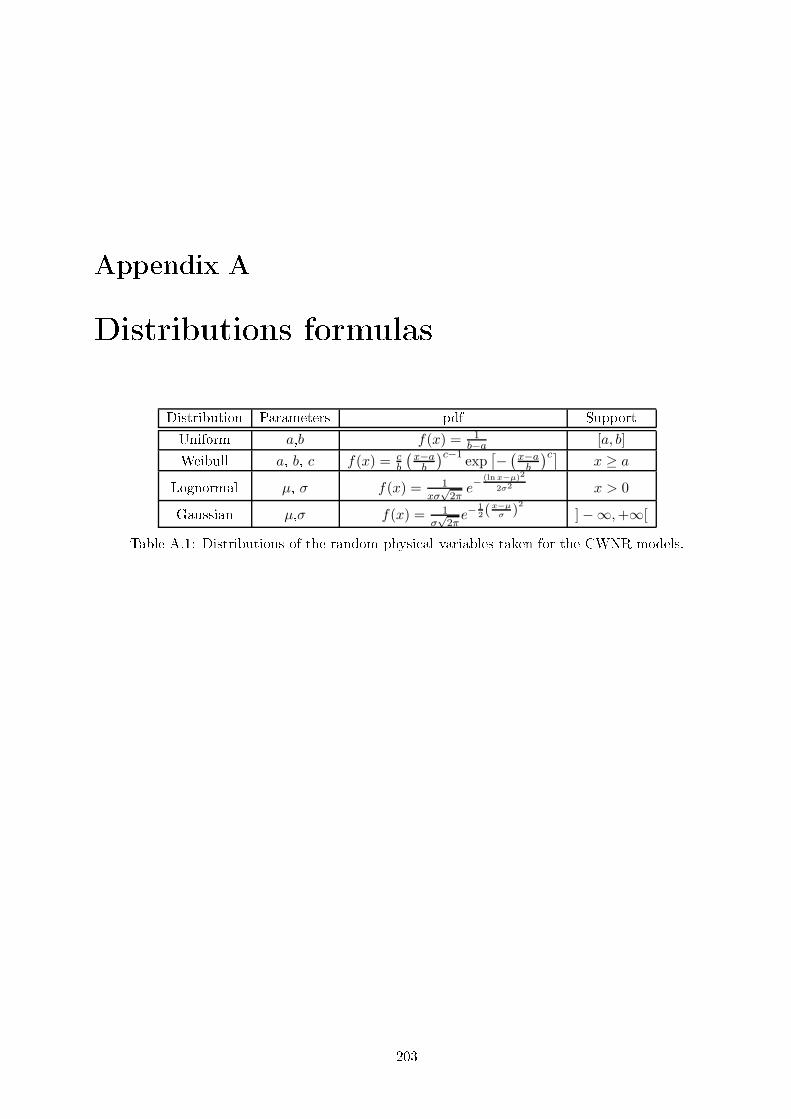
Appendix A
Distributions formulas
Distribution Parameters pdf Support
Uniform a,b f(x) = 1b−a [a, b]
Weibull a, b, c f(x) = cb
(x−ab
)c−1exp
[−(x−ab
)c]x ≥ a
Lognormal µ, σ f(x) = 1xσ
√2πe−
(lnx−µ)2
2σ2 x > 0
Gaussian µ,σ f(x) = 1σ√2πe−
12(
x−µσ )
2
]−∞,+∞[
Table A.1: Distributions of the random physi al variables taken for the CWNR models.
203

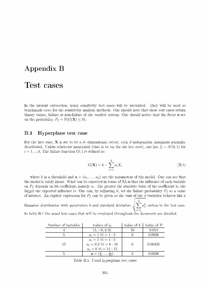
Appendix B
Test ases
In the present subse tion, usual sensitivity test ases will be presented. They will be used as
ben hmark ases for the sensitivity analysis methods. One should note that these test ases return
binary values, failure or non-failure of the studied system. One should noti e that the fo us is set
on the probability Pf = P(G(X) ≤ 0).
B.1 Hyperplane test ase
For the rst ase, X is set to be a d−dimensional ve tor, with d independent marginals normally
distributed. Unless otherwise mentioned (that is to say for the last ase), one has fi ∼ N (0, 1) fori = 1, .., d. The failure fun tion G(.) is dened as:
G(X) = k −d∑
i=1
aiXi (B.1)
where k is a threshold and a = (a1, . . . , ad) are the parameters of the model. One an see that
the model is solely linear. What an be expe ted in terms of SA is that the inuen e of ea h variable
on Pf depends on its oe ient, namely ai. The greater the absolute value of the oe ient is, the
bigger the expe ted inuen e is. One an, by adjusting k, set the failure probability Pf to a value
of interest. An expli it expression for Pf an be given as the sum of the d variables behaves like a
Gaussian distribution with parameters 0 and standard deviation
√√√√d∑
i=1
a2i , unless in the last ase.
In table B.1 the usual test ases that will be employed throughout the do ument are detailed.
Number of variables Values of ai Value of k Value of P
4 (1,−6, 4, 0) 16 0.014
5 ai = 1 ∀i = 1 : 5 6 0.0036
15ai = 1 ∀i = 1 : 5ai = 0.2 ∀i = 6 : 10ai = 0 ∀i = 11 : 15
6 0.00425
5 a = (12 , ...,110) 5 0.0036
Table B.1: Usual hyperplane test ases
205
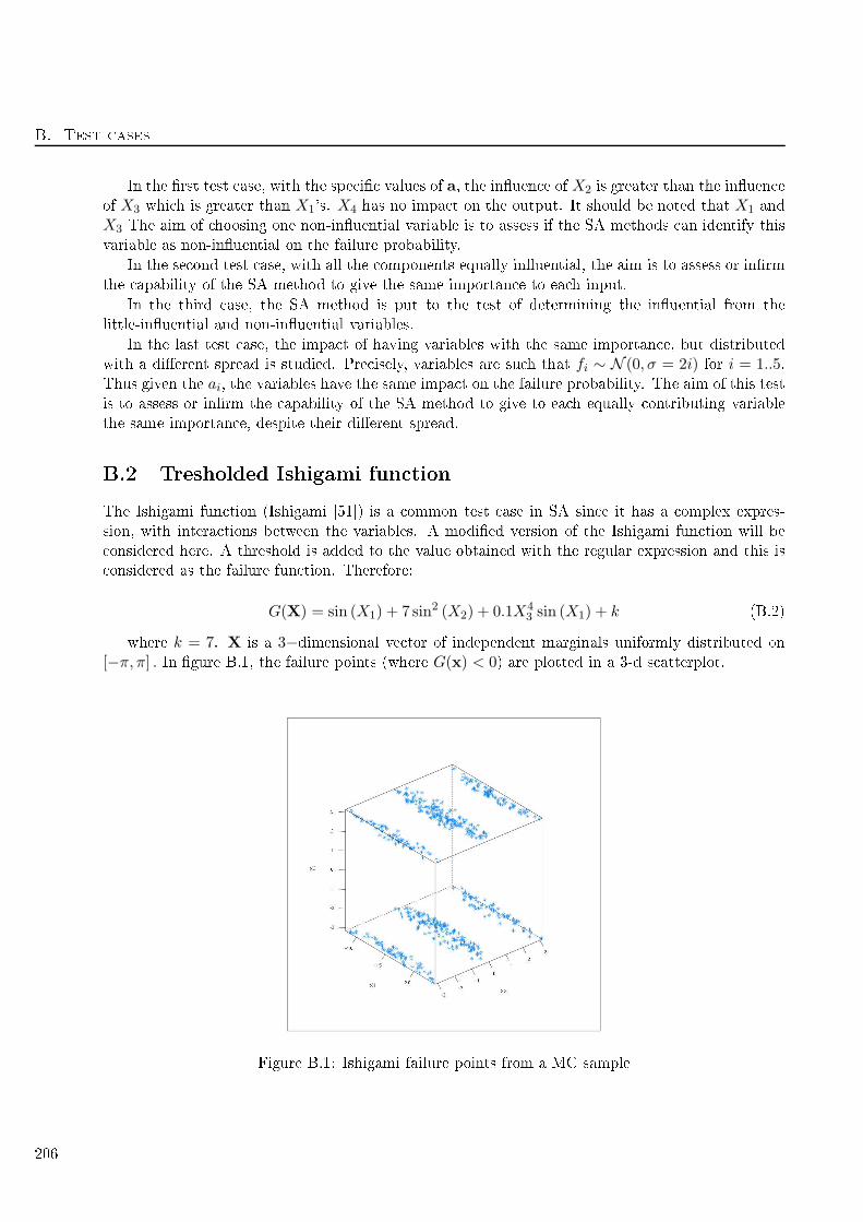
B. Test ases
In the rst test ase, with the spe i values of a, the inuen e of X2 is greater than the inuen e
of X3 whi h is greater than X1's. X4 has no impa t on the output. It should be noted that X1 and
X3 The aim of hoosing one non-inuential variable is to assess if the SA methods an identify this
variable as non-inuential on the failure probability.
In the se ond test ase, with all the omponents equally inuential, the aim is to assess or inrm
the apability of the SA method to give the same importan e to ea h input.
In the third ase, the SA method is put to the test of determining the inuential from the
little-inuential and non-inuential variables.
In the last test ase, the impa t of having variables with the same importan e, but distributed
with a dierent spread is studied. Pre isely, variables are su h that fi ∼ N (0, σ = 2i) for i = 1..5.Thus given the ai, the variables have the same impa t on the failure probability. The aim of this test
is to assess or inrm the apability of the SA method to give to ea h equally ontributing variable
the same importan e, despite their dierent spread.
B.2 Tresholded Ishigami fun tion
The Ishigami fun tion (Ishigami [51) is a ommon test ase in SA sin e it has a omplex expres-
sion, with intera tions between the variables. A modied version of the Ishigami fun tion will be
onsidered here. A threshold is added to the value obtained with the regular expression and this is
onsidered as the failure fun tion. Therefore:
G(X) = sin (X1) + 7 sin2 (X2) + 0.1X43 sin (X1) + k (B.2)
where k = 7. X is a 3−dimensional ve tor of independent marginals uniformly distributed on
[−π, π] . In gure B.1, the failure points (where G(x) < 0) are plotted in a 3-d s atterplot.
Figure B.1: Ishigami failure points from a MC sample
206
B.3. Flood ase
The failure probability here is roughly P = 5.89 × 10⁻³(estimated by Monte-Carlo te hnique,
see se tion 1.2.1). The omplex repartition of the failure points an be noti ed. Those points lay in
a zone dened by the negative values of X1, the extremal and mean values of X2 (around −π, 0 andπ), and the extremal values of X3 (around −π and π)
B.3 Flood ase
The goal of this test ase is to assess the risk of a ood over a dyke for the safety of industrial
installations (Bernardara [10). This omes down to model the level of a ood. As a fun tion
of hydrauli al parameters, many of them being randomized to a ount for un ertainty. From a
simpli ation of the Saint-Venant equation, a ood risk model is obtained.
The quantity of interest is the dieren e between the level of the dyke and the height of water. If
this quantity is negative, the installation is ooded. Hydrauli parameters are the following: Q the
ow rate, L the water ourse se tion length studied, B the water ourse width, Ks the water ourse
bed fri tion oe ient (also alled Stri kler oe ient), Zm and Zv respe tively the upstream and
downstream bottom water ourse level above sea level and Hd the dyke height measured from the
bottom of the water ourse bed. The water level model is expressed as:
H =
Q
KsB√
Zm−Zv
L
35
. (B.3)
Therefore the following quantity is onsidered:
G = Hd − (Zv +H). (B.4)
Among the model inputs, the hoi e is made that the following variables are known pre isely:
L = 5000 (m), B = 300 (m), Hd = 58 (m), and the following are onsidered to be random. Q(m
3.s−1) follows a positively trun ated Gumbel distribution of parameters a = 1013 and b = 558
with a minimum value of 0. Ks (m1/3
s
−1) follows a trun ated Gaussian distribution of parameters
µ = 30 and σ = 7.5, with a minimum value of 1. Zv (m) follows a triangular distribution with
minimum 49, mode 50 and maximum 51. Zm (m) follows a triangular distribution with minimum
54, mode 55 and maximum 56.The failure probability here is roughly P = 7.88× 10⁻⁴
(estimated by MC te hnique, see 1.2.1).
207

Appendix C
Isoprobabilisti transformations
Here, we briey introdu e the notion of opula, whi h is needed for the presentation of isoprobabilisti
transformations. Copulas are a mathemati al obje t des ribing the dependen ies in a random ve tor
without referring to the marginal distributions. Nelsen's monograph [74 presents su h obje ts.
C.1 Presentation of the opulas
Denition C.1.1 A d dimensional fun tion f is said d−in reasing if:
2∑
i1=1
· · ·2∑
id=1
(−1)i1+···+idf(x1,i1 , . . . , x2,id) ≥ 0
where xj,1 = aj and xj,2 = bj ∀j ∈ 1, . . . , d and aj , bj ∈ [0, 1], aj ≤ bj∀j ∈ 1, . . . , d
Denition C.1.2 A d−dimensional opula C is a d−dimensional umulative distribution fun tion
dened over [0, 1]d, whose marginal distributions are uniform over [0, 1]:
C is d−in reasing;
for all u ∈ [0, 1]d whi h have at least one omponent equal to 0, C(u) = 0;
for all u ∈ [0, 1]d whi h have all their omponents equal to 1 ex ept one, uk, C(u) = uk.
Theorem C.1.1 (Sklar 1959)
Let F be a d−dimensional umulative distribution fun tion with F1, . . . , Fp the marginal distri-
bution fun tions. There exists a d−dimensional opula, C, su h that for all x ∈ Rdwe have:
F (x1, . . . , xp) = C(F1(x1), . . . , Fp(xp)). (C.1)
If the marginal distributions F1, . . . , Fp are ontinuous, then the opula C is unique, otherwise it
is uniquely determined over Im(F1) × · · · × Im(Fp). In the ontinuous ase, for all u ∈ [0, 1]d we
have:
C(u) = F (F−11 (u1), . . . , F
−1p (up) (C.2)
if absolutely ontinuous
f(x) = c ((F1(x1), . . . , Fp(up))
d∏
i=1
fi(xi) (C.3)
209
C. Isoprobabilisti transformations
with c the probability distribution fun tion asso iated to C, f the probability distribution fun tion
asso iated to F and fi the marginal distributions fun tion asso iated to F .
Denition C.1.3 Let us denote SOd(R) the rotation group over Rdand supp(X) the set of the val-
ues that an be taken by a random ve tor X. An isoprobabilisti transformation T of a d−dimensional
random ve tor X is a dieomorphism from supp(X) into Rdsu h that the random ve tors U = T (X)
and rU have the same distribution for all r ∈ SOd(R).
C.2 Obje tives, Rosenblatt transformation
We wish to transform a random ve tor X of pdf fX and of opula C in a Gaussian ve tor U of same
dimension but with independent, standard Gaussian as omponents.
If the variables are independent and that the marginals are known, the transformation is straight-
forward :
ui = φ−1(Fi(xi))
If there is a dependen y stru ture in the variables, Rosenblatt and Nataf transformations are
possibilities [?.
We present here the Rosenblatt [84 transformation. This transformation is not unique if the
variables are orrelated: it depends on the order in whi h the variables are transformed
1
.
Transformation is done as follows:
u1 = φ−1(F1(x1))
u2 = φ−1(F2(x2|X1 = x1))
...
ud = φ−1(Fd(xd|X1 = x1, ...,Xd−1 = xd))
where Fi(.|X1, ...Xi−1) is the df of variable Xi given the realisations of the previous variables.
1
It has been shown in Lebrun and Dutfoy [57 that if the opula of X is Gaussian, the order in whi h the variables
are transformed does neither impa t the norm of the design point, nor the derivatives of the failure surfa e in this
point. In other words, the following quantities use in FORM/SORM methods do not depend upon the order of
transformation: βHL,PFORM , PSORM .
210

Appendix D
Appendi es for Chapter 3
D.1 Proofs of asymptoti properties
Proof of Lemma 3.2.1
Under assumption (i), we have
Supp(fiδ)1G(x)<0
fiδ(xi)
fi(xi)f(x) dx ≤
Supp(fiδ)fiδ(xi) dxi = 1.
So that, the strong LLN may be applied to PiδN . Dening
σ2iδ = Var
[1G(X)<0
fiδ(Xi)
fi(Xi)
], (D.1)
one has
σ2iδ =
Supp(fi)1G(x)<0
f2iδ(xi)
fi(xi)
d∏
j 6=i
fj(xj) dx− P 2iδ < ∞ under assumption (ii).
Therefore the CLT applies:
√Nσ−1
iδ
(PiδN − Piδ
)L−→ N (0, 1) .
Under assumption (ii), the strong LLN applies to σ2iδN . So that, the nal result is straightforwardusing Slutsky's lemma.
Proof of Proposition 3.2.1
First, note that
E
[P Piδ
]− PPiδ = E
[1
N2
(N∑
n=1
1G(xn)<0
)(N∑
n=1
1G(xn)<0fiδ(x
ni )
fi(xni )
)]− PPiδ
=1
N2E
N∑
n=1
[1G(xn)<0
]2 fiδ(xni )fi(xni )
+
N∑
n=1
N∑
j 6=i
1G(xn)<01G(xj)<0fiδ(x
ji )
fi(xji )
−PPiδ
=1
N2[NPiδ +N (N − 1)PPiδ]− PPiδ
=1
N(Piδ − PPiδ) .
211
D. Appendi es for Chapter 3
Assuming the onditions under whi h Lemma 1 is true, the bivariate CLT follows with
Σiδ =
(P (1− P ) Piδ(1− P )Piδ(1− P ) σ2iδ
).
Ea h term of this matrix an be onsistently estimated, using the results in Lemma 1 and Slutsky's
lemma.
D.2 Computation of Lagrange multipliers
Let H be the Lagrange fun tion:
H(λ) = ψi(λ)−K∑
k=1
λkδk.
Thus, using the results of Csizar [26, one has
λ∗ = argminH(λ).
The expression of the gradient of H with respe t to the jth variable is
∇jH(λ) =
gj(x)fi(x) exp(∑K
k=1 λkgk(x))dx
expψi(λ)− δj .
Similarly, the expression of the se ond derivative of H with respe t to the hth and the jth variables
is
DhjH(λ) =
gh(x)gj(x)fi(x) exp(∑K
k=1 λkgk(x))dx
expψi(λ)
−
gj(x)fi(x) exp(∑K
k=1 λkgk(x))dx
expψi(λ)
gh(x)fi(x) exp(∑K
k=1 λkgk(x))dx
expψi(λ).
This method has been used in this paper for omputing the optimal ve tor λ∗when a varian e
shifting was applied. The integrals were evaluated with Simpson's rule.
D.3 Proofs of the NEF properties
In this Appendix, the details of the al ulus for the Proposition 3.3.4 are provided.
NEF spe i ities : If the original density fi(x) is a NEF, then under a set of K linear onstraints
on f(x), one has :f(x) = b(x) exp [xθ − η(θ)] ,
thus :
fδ(x) = f(x) exp
[K∑
k=1
λkgk(x)− ψ(λ)
]
The regularization onstant from (3.13) an be written as:
ψ(λ) = log
b(x) exp
[xθ +
K∑
k=1
λkgk(x)− η(θ)
]dx (D.2)
If the integral on (D.2) is nite, fδ exists and is a density.
212
D.3. Proofs of the NEF properties
Mean shifting With a single onstraint formulated as in (3.15), (D.2) be ames :
ψ(λ) = log
b(x) exp [xθ + λx− η(θ)] dx
= log
b(x) exp [x (θ + λ)− η(θ) + η(θ + λ)− η(θ + λ)] dx
if η(θ + λ) is well dened.
ψ(λ) = (η(θ + λ)− η(θ)) + log
[
b(x) exp [x (θ + λ)− η(θ + λ)]
]dx
= η(θ + λ)− φ(θ)
sin e
b(x) exp [x (θ + λ)− η(θ + λ)] = fθ+λ(x)
with notation from (3.3.4), is a density of integral 1. Thus
fδ(x) = b(x) exp [xθ − φ(θ)] exp [λx− η(θ + λ) + η(θ)]
= b(x) exp [x [θ + λ]− η(θ + λ)] = fθ+λ(x)
Thus the mean shifting of a NEF of CDF η(.) results in another NEF with mean η′(θ + λ) = δ( onstraint) and varian e η′′(θ + λ).
Varian e shifting With a single onstraint formulated as in (3.19), using (D.2), the new distri-
bution has for density:
fδ(x) = b(x) exp[xθ + xλ1 + x2λ2 − ψ(λ)− η(θ)
]
Sin e λ is known or omputed, and θ is also known, onsider the variable hange z =√λ2x assuming
λ2 is stri tly positive (the variable hange is z =√−λ2x if λ2 is stri tly negative). Thus,
fδ(x) = b(z√λ2
) exp[z2]exp
[z√λ2
(θ + λ1)− ψ(λ)− η(θ)
]
= exp
[η
((θ + λ1)√
λ2
)− η(θ)− ψ(λ)
]c(z) exp
[z(θ + λ1)√
λ2− η
((θ + λ1)√
λ2
)]
with
c(z) = b(z√λ2
) exp[z2].
By (3.13),
ψ(λ) = log
b(x) exp[xθ + xλ1 + x2λ2 − η(θ)
]dx
= log
b(z√λ2
) exp[z2]exp
[(θ + λ1)√
λ2z − η(θ) + η
((θ + λ1)√
λ2
)− η
((θ + λ1)√
λ2
)]dx
=
(η
((θ + λ1)√
λ2
)− η(θ)
)+ log
c(z) exp
[(θ + λ1)√
λ2z − η
((θ + λ1)√
λ2
)]dx
= η
((θ + λ1)√
λ2
)− η(θ)
Thus one has :
fδ(x) = c(z) exp
[z(θ + λ1)√
λ2− η
((θ + λ1)√
λ2
)]
thus the varian e shifting of a NEF results in another NEF parameterized by
(θ+λ1)√λ2
.
213
D. Appendi es for Chapter 3
D.4 Numeri al tri k to work with trun ated distribution
In the ase where a mean shifting is onsidered on a left trun ated distribution. We present a tip
that an help to ompute λ∗.
The studied trun ated variable YT has distribution fY T . Let us denote Y ∼ fY the orresponding
non-trun ated distribution. The trun ation o urs for some real value a. This trun ation may
happen for some physi al modelling reason. One has:
fY T (y) =1
1− F (a)1[a,+∞[(y)fY (y).
The formal denition of MY T (λ) the mgf of YT for some λ is:
MY T (λ) =1
1− FY (a)
+∞
afY (y) exp [λy] dy.
Let us re all that we are looking for λ∗su h as:
δ =M ′
Y T (λ∗)
MY T (λ∗)
=
+∞a yfY (y) exp [λy] dy +∞a fY (y) exp [λy] dy
. (D.3)
When the expression does not take a pra ti al form, one an use numeri al integration to es-
timate the integral terms. Unfortunately, for some heavy tailed distribution (for instan e Gumbel
distribution), this numeri al integration might be omplex or not possible. This is due to the multi-
pli ation by an exponential of y. The following tip helps to avoid su h problems. Denoting MY (λ)the mgf of the non-trun ated distribution, one an remark that:
MY (λ) =
+∞
−∞fY (y) exp [λy] dy =
a
−∞fY (y) exp [λy] dy +
+∞
afY (y) exp [λy] dy
Thus another expression for MY T (λ) is:
MY T (λ) =1
1− FY (a)
[MY (λ)−
a
−∞fY (y) exp [λy] dy
].
The integral term is mu h smaller in the left heavy tailed distribution ase. Therefore the numeri al
integration (for instan e using Simpson's method) is mu h more pre ise or be ame possible.
The same goes for M ′Y T (λ) whi h has alternative expression:
M ′Y T (λ) =
1
1− FY (a)
[M ′
Y (λ)− a
−∞yfY (y) exp [λy] dy
].
Finally, another form of D.3 is:
δ =M ′
Y (λ)− a−∞ yfY (y) exp [λy] dy
MY (λ)− a−∞ fY (y) exp [λy] dy
. (D.4)
This alternative expression may lead to more pre ise estimations of λ∗when MY (λ) and M
′Y (λ)
are known (whi h is the ase for most usual distribution) sin e the integral term are mu h smaller
than in the rst expression.
214

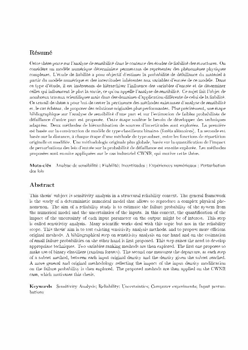
Résumé
Cette thèse porte sur l'analyse de sensibilité dans le ontexte des études de abilité des stru tures. On
onsidère un modèle numérique déterministe permettant de représenter des phénomènes physiques
omplexes. L'étude de abilité a pour obje tif d'estimer la probabilité de défaillan e du matériel à
partir du modèle numérique et des in ertitudes inhérentes aux variables d'entrée de e modèle. Dans
e type d'étude, il est intéressant de hiérar hiser l'inuen e des variables d'entrée et de déterminer
elles qui inuen ent le plus la sortie, e qu'on appelle l'analyse de sensibilité. Ce sujet fait l'objet de
nombreux travaux s ientiques mais dans des domaines d'appli ation diérents de elui de la abilité.
Ce travail de thèse a pour but de tester la pertinen e des méthodes existantes d'analyse de sensibilité
et, le as é héant, de proposer des solutions originales plus performantes. Plus pré isément, une étape
bibliographique sur l'analyse de sensibilité d'une part et sur l'estimation de faibles probabilités de
défaillan e d'autre part est proposée. Cette étape soulève le besoin de développer des te hniques
adaptées. Deux méthodes de hiérar hisation de sour es d'in ertitudes sont explorées. La première
est basée sur la onstru tion de modèle de type lassieurs binaires (forêts aléatoires). La se onde est
basée sur la distan e, à haque étape d'une méthode de type subset, entre les fon tions de répartition
originelle et modiée. Une méthodologie originale plus globale, basée sur la quanti ation de l'impa t
de perturbations des lois d'entrée sur la probabilité de défaillan e est ensuite explorée. Les méthodes
proposées sont ensuite appliquées sur le as industriel CWNR, qui motive ette thèse.
Mots- lés Analyse de sensibilité ; Fiabilité; In ertitudes ; Expérien es numériques ; Perturbation
des lois
Abstra t
This thesis' subje t is sensitivity analysis in a stru tural reliability ontext. The general framework
is the study of a deterministi numeri al model that allows to reprodu e a omplex physi al phe-
nomenon. The aim of a reliability study is to estimate the failure probability of the system from
the numeri al model and the un ertainties of the inputs. In this ontext, the quanti ation of the
impa t of the un ertainty of ea h input parameter on the output might be of interest. This step
is alled sensitivity analysis. Many s ienti works deal with this topi but not in the reliability
s ope. This thesis' aim is to test existing sensitivity analysis methods, and to propose more e ient
original methods. A bibliographi al step on sensitivity analysis on one hand and on the estimation
of small failure probabilities on the other hand is rst proposed. This step raises the need to develop
appropriate te hniques. Two variables ranking methods are then explored. The rst one proposes to
make use of binary lassiers (random forests). The se ond one measures the departure, at ea h step
of a subset method, between ea h input original density and the density given the subset rea hed.
A more general and original methodology ree ting the impa t of the input density modi ation
on the failure probability is then explored. The proposed methods are then applied on the CWNR
ase, whi h motivates this thesis.
Keywords Sensitivity Analysis; Reliability; Un ertainties; Computer experiments; Input pertur-
bations