ANALIZA NAPRĘŻEŃ SKURCZOWYCH W BETONIE Z …svf.uniza.sk/kskm/web/images/RIB/2004.pdf · Fakt...

* with the support of the Committee of Scientific Research of the Polish Government, contract No. 8 T07G 016 21

and with the partial support of the Commission of the European Communities under the FP5, contract No. G1MA-CT-2002- -04058

ROCZNIKI INŻYNIERII BUDOWLANEJZESZYT 3/2004

Komisja Inżynierii Budowlanej Oddział Polskiej Akademii Nauk w Katowicach

ANALIZA NAPRĘŻEŃ SKURCZOWYCH W BETONIE

Z UWZGLĘDNIENIEM EWOLUCJI MIKROUSZKODZEŃ*

Zbigniew PERKOWSKI

Politechnika Opolska

1. Wstęp

Powstające w betonie rozciągające naprężenia skurczowe wywołują o wiele bardziej

uszkodzenia struktury materiału w postaci mikrospękań [4,6,7,8], niż naprężenia ściskające.

Proces ten jest tutaj nie bez znaczenia, gdyż ewolucja mikrospękań ma istotny wpływ na

charakter kluczowej w prezentowanych dalszych rozważaniach relacji pomiędzy tensorem

naprężenia i odkształcenia. Z jednej strony mamy tu do czynienia ze zjawiskiem narastania

mikrospękań w betonie w kierunkach prostopadłych do kierunków rozciągających naprężeń

głównych. Fakt ten objawia się w skali makroskopowej rozwojem anizotropii betonu

[4,7,8]. Z drugiej strony, ewolucja mikrouszkodzeń wprowadza w zależności pomiędzy

naprężeniem, a odkształceniem nieliniowość [7,8], która w znacznym stopniu redukuje

poziom naprężeń. Przytoczone wyżej fakty pokazują, iż istnieje potrzeba uzależnienia

naprężeń skurczowych od ewolucji mikrouszkodzeń w betonie. Działanie takie jest

możliwe dzięki wykorzystaniu metod oferowanych przez kontynualną mechanikę

uszkodzenia, gdzie od ciągłych pól miar mikrouszkodzeń uzależnia się podatność

materiału.

2. Określenie zadanie początkowo-brzegowego

Obecnie przystąpimy do sformułowania zadania początkowo-brzegowego

pozwalającego analizować narastania naprężeń skurczowych i mikrouszkodzeń po

zakończeniu hydratacji w betonie. Z uwagi na złożoność równań opisujących rozważane

zagadnienie wprowadzone zostaną założenia upraszczające. Proces mechaniczny zawężony

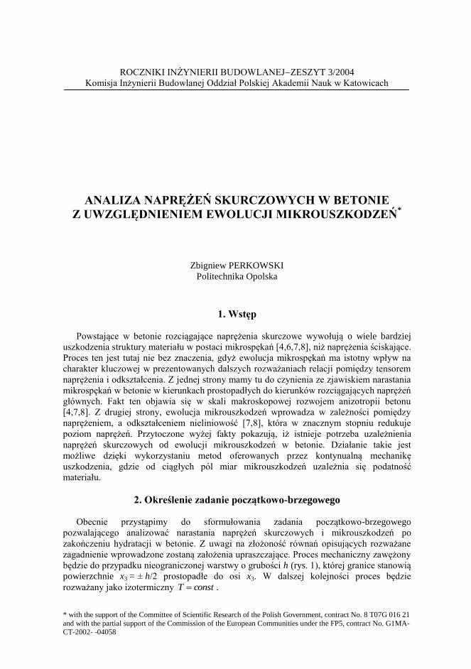
będzie do przypadku nieograniczonej warstwy o grubości h (rys. 1), której granice stanowią

powierzchnie x3 = ± h/2 prostopadłe do osi x3. W dalszej kolejności proces będzie

rozważany jako izotermiczny constT .

Z kolei, skurcz materiału zaczyna się od krytycznej koncentracji wilgoci materiału ckrw

[2] - to jest takiej, poniżej której zanika przepływ kapilarny wilgoci w fazie ciekłej. Wtedy,

jeśli w analizowanym przykładzie przyjąć, że w chwili początkowej koncentracja wilgoci

będzie równa krytycznej w obrębie całej warstwy, to proces wysychania betonu zawężony

będzie do jednokierunkowego przepływu wilgoci prostopadle do płaszczyzny warstwy.

Sytuacja taka implikuje fakt, iż funkcja opisująca koncentrację wilgoci będzie uzależniona

w przestrzeni tylko od zmiennej x3, a równanie transportu wilgoci uprości się do przypadku

,033 w

,

w jc w,eff

w cDj 33 , 0 ,22

,, 3 th

xh

ctxc w

kri

w*. (1)

Warunek brzegowy będzie określony tutaj poprzez wartości strumienia wilgoci na

powierzchni zewnętrznej, analogicznie do prawa Newtona wymiany ciepła przez

konwekcjęe przy zachowaniu stałej wilgotności względnej otaczającego powietrza θ=const

www ccat,xj 33, 0 ,

23 t

hx . (2)

Natomiast w stronie mechanicznej problemu nieznane pola przemieszczeń ui,

odkształceń εij i naprężeń ζij wyznaczymy z następującego układu równań równowagi,

równań geometrycznych i równań fizycznych (dla uproszczenia w zadaniu pominiemy

wpływ sił masowych ρFi i zewnętrznych obciążeń mechanicznych Pi)

0j,ij , (3a)

i,jj,iij uu 2

1 , ,s

ij

D

ij

v

ij

e

ijij (3b)

kl*ijkl

Dij

sij

Dijklijklij σAεεdtF D ,* , wws

ijsij cc * (3c)

gdzie:

, 2

1

,

0

0

0

021 jkiljlikklijjkiljlikklijijkl

ikjliljkjkiljlikklijklij

*

ijkl

EEtJtJtF

DDDDDDA

(4)

W równaniu fizycznym (3c) wpływ uszkodzeń na odkształcalność materiału został

uwzględniony za pomocą tensora czwartego rzędu A*

ijkl, wyrażającego ortotropową zmianę

podatności materiału podlegającego mikrospękaniom. Jego forma została podana w oparciu

o teorię funkcji reprezentacji tensorowych i ograniczona do liniowej zależności względem

tensora efektu uszkodzenia Dij [7]. Zapis (3c), w tym ujęciu, wyraża de facto

odkształcalność materiału sprężysto-kruchego uogólnioną do przypadku liniowo

lepkosprężystego [6]. Występujący w powyższych zapisach tensor efektu uszkodzenia Dij

obliczony będzie na podstawie równania ewolucji tensora uszkodzenia ij [9]

zaproponowanego przez Litewkę [7], w którym dla zróżnicowania wpływu pomiędzy

ściskaniem i rozciąganiem na rozwój mikrospękania materiału wprowadzono redukcję

głównych składowych ujemnych tensora naprężenia [8]

ijklklijklklij DsCs , 1,0ij , przy czym 3,2,1 ,1 p/D ppp (5)

Dużym uproszczeniem będzie tu przyjęcie, że proces pełzania jest niezależny od poziomu

mikrouszkodzeń, a w chwili początkowej t=0 rozpatrywane ciało jest izotropowe i nie

zawiera mikrouszkodzeń. Wówczas pola naprężeń w przedstawionym zadaniu początkowo-

brzegowym nieograniczonej warstwy mogą być wyznaczone w oparciu o równania

naprężeniowe, które po przekształceniach można zredukować do jednej zależności

tBxtAd*tFtF Ds

131111111221111 (6)

Funkcje czasu A1(t) i B1(t) należy wyznaczyć z warunków globalnej równowagi warstwy

0 , 02

2

3311

2

2

311

/h

/h

/h

/h

dxxdx . (7)

W dalszej kolejności rozważymy przypadek szczególny procesu, gdzie

t

ijklijkl etgtHtgd*tfFtftF101

1

1 , , . (8)

Rys.1 Geometria problemu

Fig.1 Geometry of the problem

Z uwagi na fizyczną nieliniowość wprowadzoną w powyższym równaniu, w wyniku

uwzględnienia procesu ewolucji uszkodzenia, w celu obliczenia naprężenia 11=22 należy

wykorzystać przyrostową formę równania (6)

6. Wyniki i wnioski

Z uwagi na przyrostowe przedstawienie problemu obliczenia naprężeń i uszkodzeń

przeprowadzono za pomocą własnych procedur obliczeniowych w środowisku programu

Matlab. W przykładzie obliczeniowym przyjęto, iż warstwa wykonana jest z betonu B30 o

grubości h=0.2[m]. Potrzebne parametry materiałowe do rozwiązania zagadnienia przyjęto

na podstawie [1,2,3,7,8,10] równe: E0=30800[MPa], 0=0.19[-], =0.1[-], fcm=28.14[MPa],

fctm=2.22[MPa], =-1.457510-6

[MPa-1

], =6.205410-6

[MPa-1

], C/2=1.84510

-3[MPa

-2],

D/2=2.979110

-4[MPa

-2], 602. [-], 0=0.03[-], α

s=310

-3[-], Deff=1.3910

-9[m

2/s],

a=5.5510-8

[m/s], ckrw=0.020[-], θ=60[%], c

∞w=0.011[-]. Uzyskane wyniki przedstawiono

na rys. 2-5. Zmiany koncentracji wilgoci po grubości warstwy wyznaczone według [5]

zamieszczono na wykresie na rys. 2. Wywołały one samozrównoważone pola naprężeń

skurczowych. Przebieg w czasie ekstremalnych naprężeń rozciągających, na zewnętrznych

powierzchniach warstwy, obliczony porównawczo według podejścia sprężystego,

sprężystego z uszkodzeniem i lepkosprężystego z uszkodzeniem przedstawiono na rys. 3.

D22

33

Fi=[0,0,0]

-siła masowa

Pi=[0,0,0]

-obciążenie

zewnętrzne

Stan odkształcenia 33=33(x3,t)

Stan naprężenia

11=11(x3,t)= 22(x3,t)

Dij( t=0)=0

-uszkodzenie w chwili

początkowej

V

s33

s11

Odkształcenia

skurczowe s

11=s22=

s33=

s(x3,t)

s22

11

h

22

Stan uszkodzenia D11=D11(x3,t)=D22(x3,t)

D33=D33(x3,t)

D33

D11

cw=cw(x3,t)

-koncentracja wilgoci

T=const -temperatura

=const -wilgotność względna

powietrza

F

x1

x3

x2

cw

-końcowa koncentracja

wilgoci

jwi=[0,0,jw

3]

-strumień wilgoci

jwi=[0,0,jw

3]

-strumień wilgoci

Rys. 2 Wykresy koncentracji wilgoci cw po grubości warstwy przy wilgotności względnej

powietrza =60[%] w chwili początkowej oraz po 1, 8, 34 i 134 dobach

Fig. 2 A diagram of moisture concentration cw along thickness of the layer at relative

humidity of air =60[%] in the initial moment and in 1, 8, 34 and 134 days

Rys.3 Przebieg naprężeń skurczowych 11 i 22 na powierzchni warstwy x3=h/2

Fig.3 A course of shrinkage stresses 11 and 22 on the surfaces of layer x3=h/2

Rys.4 Przebieg składowych tensora uszkodzenia 11 i 22 na powierzchni warstwy x3=h/2

Fig.4 A course of components 11 and 22 of the damage tensor on the surfaces of layer

x3=h/2

10 -2 10 -1 10 0 10 1 10 2 0

0.2

0.4

0.6

0.8

1

ewolucja uszkodzenia bez uwzględnienia

pełzania

ewolucja uszkodzenia

z uwzględnieniem pełzania

t[doba]

11,22

[-]

analiza lepkosprężysta z uszkodzeniem-

maksymalne naprężenie w 46 godz. analiza sprężysta z uszkodzeniem-

zarysowanie po 36 godz.

analiza sprężysta-

zarysowanie po 8 godz.

11/fctm

22/fctm

[-]

10 -2

10 -1

10 0

10 1

10 2 0

0.2

0.4

0.6

0.8

1

t[doba]

-h/2=-0.1 -0.05 0 0.05 h/2=0.1 0

2

4

6

8 9

x3[m]

c =cw-c

w

[-] x 10-3

t=1[doba] t=0 t=8[doba]

t=34[doba]

t=134[doba]

=60[%] =60[%]

Rys.5 Wykresy maksymalnych naprężeń skurczowych 11 i 22 po grubości warstwy w 46

godz. (analiza lepkospężysta z uszkodzeniem).

Rys.5 A diagram of shrinkage stresses 11 and 22 among thickness of the layer in 46 hour,

(viscoelastic analysis with damage).

Z porównania wyników widać, iż naprężenia skurczowe uzyskane w analizie sprężystej

osiągają na powierzchni wartość równą fctm po czasie 8[h], a w analizie sprężystej z

uszkodzeniem po czasie 36[h]. Natomiast w analizie lepkosprężystej z uszkodzeniem

naprężenia te maksymalną wartość równą ok. 0.92fctm osiągnęły po czasie 46[h]. Należy

zwrócić tu uwagę, iż proces relaksacji naprężeń przyczynia się do zmniejszenia poziomu

uszkodzenia, co można zauważyć po zmianach w czasie składowych tensora uszkodzenia

ij zamieszczonych na rys. 4. Z zaprezentowanych wyników można także wywnioskować,

iż kumulacja mikrouszkodzeń w strefach przypowierzchniowych warstwy, w wyniku

działania naprężeń rozciągających, będzie prowadzić przy cyklicznym namakaniu i

wysychaniu materiału do rozwoju makrospękań. Stąd, prezentowany model obliczeniowy,

po uogólnieniu go dla dowolnych warunków hygrotermicznych otoczenia, może służyć do

przewidywania trwałości elementów wykonanych z materiałów skałopodobnych.

Oznaczenie symboli

a- współczynnik przejmowania wilgoci, moisture transfer coefficient, [m/s],

cw, ckr

w, c

*w, c

∞w- masowa koncentracja wilgoci: bieżąca, krytyczna, początkowa i

równowagowa dla wilgotności względnej powietrza θ, current, critical, initial and

equilibrium for relative humidity of air θ mass moisture concentration, [-],

fcm, fctm - wytrzymałość na ściskanie i rozciąganie, compression and tensile strength, [Pa],

jiw- całkowity strumień wilgoci, total flux of moisture, [kg/(m

2s)]

t, η – czas i wiek, time and age, [s]

ui- wektor przemieszczenia, displacement vector, [m]

A*ijkl- tensor zmiany podatności spowodowanej ewolucją uszkodzenia w materiale, tensor of

change of compliance caused by damage evolution in material, [Pa],

C,D- stałe materiałowe, material constants, [Pa-2

],

Deff – efektywny współczynnik dyfuzji wilgoci, effective moisture diffusivity, [m2/s],

Dij- tensor efektu uszkodzenia, damage effect tensor, [m2/m

2],

E0- początkowy moduł Younga, initial Young’s modulus, [Pa],

Fi- wektor sił masowych, mass forces vector, [N/m3],

Fijkl, Fijkl(t)- tensor podatności i funkcji pełzania, compliance and creep functions tensor,

[Pa-1

],

J1, J2- funkcje pełzania, creep functions, [Pa],

Pi- wektor obciążeń powierzchniowych, surface load vector, [N/m2]

T- temperatura, temperature, [oK]

-h/2=-0.1 -0.05 0 0.05 h/2=0.1 -0.2

0

0.2

0.6

1 11/fctm

22/fctm

[-]

x3[m]

α, γ- stałe materiałowe, material constants, [Pa-1

]

αs- współczynnik skurczu, shrinkage coefficient, [-],

γ0- stała materiałowa, material constant, [-],

δij- delta Kroneckera, Kronecker’s delta,

εij, εije, εij

v, εij

D, εij

s- tensor odkształceń: całkowitych, sprężystych, lepkich, wywołanych

uszkodzeniem materiału oraz skurczowych, total, elastic, viscous, caused by material

damage and shrinkage strain tensor, [-],

0- współczynnik Poissona, Poissons’s ratio, [-],

ρ- gęstość materiału, density of material, [kg/m3],

ζij, skl - tensor i dewiator naprężenia, stress tensor and deviator, [Pa]

- współczynnik pełzania, creep coefficient, [-],

Ωij- tensor uszkodzenia, damage tensor, [m2/m

2],

(...)+- redukcja składowych głównych ujemnych tensora do części wyrażonej przez stałą ζ,

reduction of negative principal components of tensor to part expressed by constant ζ.

Literatura

[1] Aleksandrowski S.W.: O nasljedstwiennych funkcjach tieorii połzučesti starjejušciewo

bietona, Połzučest stroitielnych matieriałów i konstricii, Strojizdat, Moskwa, 1964

[2] Aleksandrowski S.W.: Rasčiot bietonnych i železobietonnych konstrukcji na

temperaturnyje i włažnostnyje wozdiejstwa, Strojizdat, Moskwa, 1973

[3] Arutiunian N.C.: Niektoryje woprosy tieorji połzučesti, Gos. Izdat. Tiech.-Teor. Lit.,

Moskwa-Leningrad, 1952

[4] Chen W.F.: Plasticity of reinforced concrete, McGrow-Hill, New York, 1982

[5] Kącki E.: Równania różniczkowe cząstkowe, WNT, Warszawa, 1989

[6] Kubik J., Perkowski Z.: Description of brittle damages to concrete, Proc. Int.

Symposium ABDM, Kraków-Przegorzały, 2002

[7] Litewka A., Bogucka J., Dębiński J.: Analitycal and experimental study of damage

induced anisotropy of concrete, ZN Politechniki Poznańskiej, Nr 45, S. Budownictwo

Lądowe, Poznań, 2001

[8] Murakami S., Kamiya K.: Constitutive and damage evolution equations of elastic brittle

materials based in irreversible thermodynamics, Int. J. Solids Struct., 39, s. 437-486,

1997

[9] Murakami S., Ohno N.: A continuum theory of creep and creep damage, Creep in

Structure, IUTAM Symp. Leicester, ed. A.R.S. Ponter D.R. Hayhurst, Springer, Berlin,

s. 422-443, 1981

[10] PN-B-03264:1999, Konstrukcje betonowe, żelbetowe i sprężone, 1999

Analysis of shrinkage stresses in concrete with damage evolution

Summary In the work analysis of shrinkage stresses together with damage evolution leading to

anisotropy in concrete is presented. The model of multicomponent body with a dominant

constituent and damage mechanics are employed to describe the process. To simplify

considerations the following assumptions are introduced: isothermal conditions hold,

concrete is isotropic body in the initial moment with ended process of hydration and

humidity of concrete is equal to the critical one.



VISCOELASTIC BENDING OF R-C PLATE BY FSM

Jozef SUMEC

1,2, Ivana VÉGHOVÁ

1

1Slovak University of Technology

2University of Saint Cyril and Methodius, Trnava

1. Abstract

In this paper the bending of R-C plate is analyzed. The material properties of reinforced

concrete slab is modelled as a viscoelastic media. The thermorheological simple material is

supposed. The linear viscoelastic problem has been solved by means of the so-called visco-

elastic analogy in the sense of the Laplace transformation owing to which the calculation

splits into three stages: - suggestion of the optimum solution of the associated elastic

problem, - sufficiently adequate simulation of the time-dependent properties of materials,

and – use of the Laplace integral transformation and its numerical inversion. Numerical

example of the plate by finite strip method.

2. Introduction

In this contribution the stresses and corresponding deformations of plate structure made

from viscoelastic composite material are analysed. The physical properties of the used

material according to the linear theory of viscoelasticity (in the sense of Laplace transform)

are described. The viscoelastic properties of composite material are modelled by

rheological models (e.g. R.M. Christensen [1]) and theory of reinforcing (e.g. A. K.

Malmeister [2]). In the solution of the problem so-called viscoelastic analogy is used.

As M. A. Biot [3] showed that in the case of homogeneous relaxation spectra similarly

as in isotropic bodies the deformations of anisotropic bodies are the same as in elastic

bodies under of transform loads and stresses are same as in elastic bodies. As was showed

by J. Brilla [4] that in the case of general relaxation spectra the viscoelastic analogy in the

sense of Laplace transformation is possible to use.

The solution of the associated boundary value problem is equivalent to the problem of

minimisation of the general potential energy. The inverse transform is obtained numerically

in the form of the Dirichlet series. The particular material of the structure is characterised

by the visco-elastic coefficients which are function of time-parameter.

3. Derivation of the material tensor-operator

In this case we shall consider a standard linear viscoelastic material. We assume that the

Maxwell element of the “three parameters” linear viscoelastic material, also called Zener´s

material has a homogeneous relaxation spectrum

ijklijkl EK (1)

where K is the inverse value of the relaxation time of the structure material. Scheme of the

Zener´s model with a homogeneous spectra of a Maxwell element is given in Fig. 1.

ijklE

2

ijklE1

ijkl2

Fig.1 Zener´s model

According to e.g. A. K. Malmeister [5] this model is appropriate under some

simplifications for the expression of the viscoelastic properties of concrete.

The differential equation of the rheological model has a form

KEEEK

121 (2)

By applying the Laplace transformation to equation (2) where 1 iip is the i-th

parameter of the Laplace transform and tildes denote the results of the transformation (see

e.g. H. S. Carslaw and J. C. Jaeger [6]) we obtain

klijklijklijklij EKEEpKp ~~1

121

1 (3)

In contracted form, if we denote ijijij EEE21

we obtain for orthotropic material (S.

Lichardus and J. Sumec [7]) relationships

12661

6612

22221

2211

121

1222

22121

1211

111

1111

11

111

111

~~

~~~

~~~

EK

pEK

p

EK

pEEK

pEK

p

EK

pEEK

pEK

p

(4)

or in the compact form

klijij d

Kp ~~

11

(5)

In the equation (5) for tensor-operator ijd follows

661

66

221

22121

12

121

12111

11

100

011

011

EK

pE

EK

pEEK

pE

EK

pEEK

pE

d ij (6)

The stresses in the elastic orthotropic two-dimensional structure are obtained from the

well-known equation

klijklij c (7)

where operator [cijkl

] depends on the arrangement of reinforcing bars or fibres. More details

see in J. Sumec [8].

4. Mathematical model of the problem analyzed

In this part we shall deal with the quasistatics solution of the reinforced structural

elements, considered as a layered visco-elastic orthotropic media. In the cross-section

analysed structural element should be divided in to the finite number of layers with

different material characteristics. Material characteristics of each layer by rheological

models and reinforcing theory are described.

From the mathematical point of view we are solving the boundary value problem theory

of visco-elasticity for parabolic partial differential equations. It is necessary to find the

system of vector-functions wm (P,t) for m=1,2,...,r (r is the total number of layers), such that

for every t > 0 the operator equation is fulfilled

Lwm=f (8)

in domain ,; 3Em

m

which is closed by smooth piecewise continuous

surface

m

mSSS .

System of the solution tPwm , have to be continuous in closed region

StP ;; 0 and satisfy following supplementary conditions

0mw on S and (9)

omm wPw 0, for on0t (10)

Expression

21 LLL

t and are partial differential operators.

Considering the initial condition (10) and simultaneously using the integral Laplace

transformation in form

dtetPwpPw pt

0

,,* (11)

on Eq.(1), we can this equation to express in the sense of associated elastic problem by the

formula ** fwm *L (12)

where 21 LLL ** p and for Rp the operator *L is positively definite, so that

***** ,, mmmm wwww 2L (13)

According to e.g. S. G. Michlin [9] our problem is equivalent to the problem finding the

system of elements 22Wwm

* for which

min,, ****** mmmm wfwww FL 2 (14)

from which implies the weak solution. Energy functional is minimizing on the finite

dimensional space VN of the basic function S, where 22WVN .

Let is given the set NyYzxXzyx imimim ,...,,,,, 21 as a product of polynomial-

trigonometric functions (base of space VN). In this space we shall construct the linear

combination of N coordinate elements

im

N

iimNm

w

1

** (15)

where *im are coordinates of *

mNw with respect to the im , i-is the index of layer.

After substitution of Eq. (15) into Eq. (14) we have an approximation of *

mNwF in the

form of quadratic functional as follows

****

,

,,mN

N

kmkkmim

N

kjmkj wf F

1

2 (16)

From the theory of minimum quadratic functional (because *L is positively definite

operator) implies the equivalence between elements of space VN and 22W in form

min; *** mNim wfw FL* .

Necessary conditions for minimum of *

mNwF giving the one-parametric (with respect

to p ) system of linear algebraic equations

0

*

*

im

Nmw

F (17)

for unknowns *im .

In the matrix form the energy functional have a form (in Laplace image)

******** UWTT fδδKδδ2

1F (18)

where *F is an energy functional, W* is potential energy of the external load, U

* is

a deformation work and K is a stiffness matrix of the analyzed structure. After solution of

associated elastic problem it is important to use the algorithm of inverse Laplace

transformation and consequently time-dependent fields of stresses and displacement.

5. Numerical example

In this example we shall investigate the reinforced concrete bridge – type simply

supported plate under uniformly distributed vertical load of intensity q = 3.43 kN/m2 . The

dimensions of the analyzed plate were 0.12m x 1.20m x 3.60m. The “cross-section” of the

plate 0.12m x 1.20m was divided into two layers (Fig.2) where h1 = 6.20cm and h2 =

5.80cm with depth h2 (bellow the neutral plane) where we considered weaken by cracks and

microcracks. The material matrix was derived according to the method shown as above in

Part 3. For identification of final results the numerical algorithm of the inverse Laplace

transform was used. The course of vertical displacements of the central point plate with

respect to the time t were controlled. Theoretically obtained results with experimental

measurement made after 30 days and 900 days [10] were compared. The second result of

deflection was treated as a deflection for t→∞. The general course of vertical displacements

of the central point of plate with respect to the time t (days) is illustrated in Fig. 2.

Fig.2 Time-dependent course of plate central point deflection

By the full and empty triangles or squares the upper and lower limits of the deflections

obtained from twelve experimental measurement on the real model after 30 days and 900

days are marked. The above described numerical method enables us to predict the long time

deflections of reinforced concrete elements on the basis of experimentally measured basic

material properties.

List of symbols

ijklE ,

ijkl -tensor of module of elasticity and viscosity

-Green-Saint Venant strain tensor

-Piola-Kirchhoff stress tensor

p -parameter of Laplace transformation

tPwm , -system of vector-functions

E3 -Euclidean 3D space

-domain of the body analyzed

L -partial differential operator

22W -functions vector space with prescribed properties

im -system of basic functions

F -energy functional

References

[1] Christensen R.M.: Theory of Viscoelasticity. New York, Academic Press 1971.

[2] Malmeister A. K. et al: Strength of Polymers. Riga, Izdat. ZINATNE 1972.

[3] Biot M. A.: Variational and Lagrangian Methods in Viscoelasticity Deformation and

Flow of Solid. In: IUTAM, Coll., Madrid 1955, Springer Verlag 1956.

[4] Brilla J.: Convolutional In: Proc. Int. Conf. Var. Method in Engng., Southampton 1972.

[5] Malmeister A. K.: Elasticity and Inelasticity of Concrete. (In Russian). Riga.

[6] Carlslaw H. S., Jaeger J.C.: Operational Methods in Applied Mathematics. London,

Oxford University Press 1948.

[7] Lichardus S., Sumec J.: Analysis of structural elements of various dimensions made

from composite viscoelastic materials. (In Slovak). Internal Research Report of Institute

of Construction and Architecture of the SAS, Bratislava 1978.

[8] Sumec J.: State of stress and strain in structural elements and systems made from linear

visco-elastic materials. (In Slovak). Internal Research Report of Institute of

Construction and Architecture of the SAS, Bratislava 1985.

[9] Michlin S. G.: Variational methods in mathematical physics. (In Russian). Moscow,

Gostechizdat 1957.

[10]Hájek J. et al: Influence of steels with higher mechanical properties on the limit state of

serviceability of planar structures under long-time loading. Internal Research Report of

Institute of Construction and Architecture of the SAS, Bratislava 1980.

VÄZKOPRUŽNÝ OHYB ŽELEZOBETÓNOVEJ DOSKY

POMOCOU MKP

Summary V danom článku sa zaoberáme analýzou ohybu železobetónovej dosky od účinku

dlhodobého kvázistatického zaťaženia. Materiál železobetónovej dosky je modelovaný

trojprvkovým Zenerovým reologickým modelom, s využitím teórie armovania.

Z matematického pohľadu je úloha formulovaná v zmysle nájdenia slabého riešenia

energetického funkcionálu na konečnorozmernom podpriestore funkcií z 22W . Aplikovaná

je väzkopružná analógia v zmysle Laplaceovej integrálnej transformácie. Získané

numerické riešenie je porovnané s nameranými hodnotami z experimentálneho modelu.

V riešení bol použitý vlastný program STRIP, ktorý riešil úlohu metódou vrstevnatých

konečných pásov (FSM).



TEORETYCZNY OPIS I BADANIA EKSPERYMENTALNE

PROCESU REALKALIZACJI

SKARBONATYZOWANEGO BETONU

Mariusz JAŚNIOK, Adam ZYBURA

Politechnika Śląska, Gliwice

1. Wprowadzenie

Podczas elektrochemicznej realkalizacji skarbonatyzowanego betonu zachodzą

złożone zjawiska chemiczne, które w sposób zasadniczy zmieniają właściwości otuliny

betonowej [1, 2, 3]. Schemat realkalizacji przedstawiono na rys. 1.

22 22-- ++

+

A: 2 H O - 4 e = 4 H + OA: 2 H O - 4 e = 4 H + O

H

23

2

- -OH CO

+

+

+Na

K

Ca

4

32

22 22-- --K: 2 H O + 2 e = 2 OH + HK: 2 H O + 2 e = 2 OH + H

1

Rys. 1. Schemat przemian chemicznych w betonie podczas realkalizacji – opis w tekście

Fig. 1. Scheme of chemical changes in concrete being realkalized – description in the text

Głównym źródłem przemian w strukturze betonu jest zewnętrzne pole elektryczne

wytwarzane pomiędzy zbrojeniem 1 a metalową siatką 2 umieszczaną na powierzchni

betonu w alkalicznym elektrolicie 3. Na powierzchni zbrojenia 1 powstają jony OH,

natomiast na siatce anodowej 2 tworzą się jony H+. Jony te wraz z innymi jonami

zawartymi w cieczy porowej betonu przepływają w kierunku siatki anodowej 2 lub

zbrojenia 1. W strukturę otuliny wnikają także jony Na+ z zewnętrznego elektrolitu 3,

2

będącego roztworem Na2CO3. Zwiększenie liczby jonów wodorotlenowych oraz jonów

sodu wpływa na wzrost obniżonego wskutek karbonatyzacji odczynu zasadowego cieczy

porowej i powoduje odbudowę ochronnej warstewki pasywnej na powierzchni stali oraz

powstrzymanie korozji zbrojenia.

W pracy przedstawiono model procesu realkalizacji skarbonatyzowanego betonu,

opracowany na podstawie teorii ośrodka wieloskładnikowego [4, 5, 6] oraz omówiono

wyniki badań eksperymentalnych zmian koncentracji podstawowych jonów w cieczy

porowej wskutek tego zabiegu.

2. Równania procesu realkalizacji

c)b)a)

Ca2

6

1 2

23

4

e)

f)

w

w

v

v

v

u

v

v

x

x

x

0

2

0

1

3

A

“X”

V

=2,3

=7,8

=1,4

=0

5,6

K5 Na

2CO

4

3

2

OH1

H3

“X”

d)

6

5

2

“X”

Rys. 2. Wieloskładnikowy model procesu realkalizacji – opis w tekście

Fig. 2. Multi-component model of realkalization process – description in the text

Do analitycznego opisu procesu zastosowano równania termomechaniki ośrodka

wieloskładnikowego według [4, 5, 6]. Uwzględnia się, że poddawane realkalizacji otulenie

betonowe (rys. 2a) składa się z kruszywa 1 złączonego stwardniałym żelem cementowym 2

(rys. 2b). W żelu cementowym 2 występują pory kapilarne 3 połączone porami żelowymi 4

(rys. 2c). Z otuliny wydziela się cząstkę X, zawierającą pory z zaadsorbowaną na ich

ściankach cieczą 5 i osadzonymi produktami karbonatyzacji 6 (rys. 2d). Podstawowe

składniki procesu: 1 jony OH, 2 jony Na

, 3 jony H

, 4 jony CO3

2, 5 jony K

, 6

jony Ca2

, 7 – cząsteczki O2 oraz 8 – cząsteczki H2 przemieszczają się w cieczy porowej.

Całą wydzieloną cząstkę modeluje się ośrodkiem zawierającym nieruchomy szkielet = 0

oraz ruchome składniki – jony ujemne = 1, 4, jony dodatnie = 2, 3, 5, 6 oraz cząsteczki

elektrycznie obojętne = 7, 8 (rys. 2e). Uwzględnia się gęstość masy poszczególnych

składników oraz wektory prędkości całkowitej v, a następnie prędkość całkowitą

rozdziela się na prędkość środka ciężkości masy w i prędkość dyfuzyjną u (rys. 2f).

Globalny bilans masy każdego składnika określa równanie

3

VV

dVRdVdt

d, = 0, 1, 2,…, 8. (1)

Po uwzględnieniu związków

, uwv , uj , C , (2)

równanie (1) sprowadza się do parcjalnego równania bilansu masy

jdivRdt

dC

. (3)

Migracji jonów towarzyszy przepływ ładunku elektrycznego. Uwzględniając, że jednostka

masy jonów przenosi stałą liczbę ładunków elektrycznych e, globalny bilans ładunku

elektrycznego składnika określono równaniem

V V

RedVedt

d, = 0, 1, 2, 3,…, 6. (4)

Po przekształceniach i podstawieniu zależności

ji e ,

ee ,

ii ,

0Re , (5)

uzyskuje się związek

0divρedivt

e

iw

)(. (6)

Poszczególne składniki znajdujące się w otulinie betonowej są poddane działaniu sił –

rys. 3. Związek między siłami istniejącymi w cząstce X ujmuje równanie bilansu pędu

V AV

ddVdvvdt

dAPFF e . (7)

dtdw

dA

x

x

x

1

e

2

3

A

X

V

P

F

F

F

n

=1,2,3

=7,8

=0

4,5,6

Rys. 3. Schemat sił działających na składniki procesu

Fig. 3. Scheme of forces as acting on process components

Określając siłę działania pola elektrycznego wzorem Lorentza oraz uwzględniając

zależności

nσP ,

σσ , 0dt

d

w, (8)

równanie bilansu pędu upraszcza się do postaci

0div σEF e . (9)

4

Procesy zachodzące w otulinie poddawanej działaniu pola elektrycznego wywołują zmiany

energetyczne, które wyraża się równaniem bilansu energii

,, 0Kd

dVErdVKUdt

d

VV

A

AqvP

vFF e

(10)

Do przekształconego wyrażenia (10) podstawia się równania bilansu pędu (9) i równania

bilansu masy (3), wykonuje się sumowania

dt

dU

dt

dU

,

rr

,

qq

, (11)

i po uwzględnieniu równań Maxwella, równanie bilansu energii (10) sprowadza się do

postaci

.egraddt

dC

Rdivrdt

dU

wEDEj

d:σq

ΜΜ

Μ

(12)

W powyższym wyrażeniu

σtrUΜ , (13)

oznacza potencjał elektrochemiczny składnika .

Ponieważ proces elektrodyfuzji składników w otulinie ma charakter nieodwracalny, więc

musi być spełniona nierówność wzrostu entropii

V V

dT

dVRMrT

1dVS

dt

d

A

Aq

. (14)

Do nierówności (14) podstawiono równanie bilansu energii (12) oraz wprowadzono

równanie konstytutywne, wyrażające energię wewnętrzną U, entropię S i natężenie pola

elektrycznego E za pośrednictwem nowej funkcji – energii swobodnej A

ED STUA . (15)

Uwzględniając, że energia swobodna A jest funkcją parametrów procesu: koncentracji

składników C, temperatury T, natężenia pola elektrycznego E oraz odkształcenia

),,T,C(A εE Α , (16)

określono jej pochodną względem czasu t

t

A

t

A

dt

T

T

A

dt

dC

C

A

dt

dA

ε

ε

E

E, (17)

a następnie końcową postać nierówności rezydualnej

.0TgradT

gradeA

dt

d1A

dt

dTS

T

A

dt

dC

C

A

qjwEd:σ

ε

ED

E

Μ

Μ

(18)

5

Na podstawie własności nierówności rezydualnej ustala się warunki ograniczające

,A

,A

,T

AS,

C

A

εσ

ED

Μ (19)

.0Tgrad,0grad qj Μ (20)

Z warunków tych wynikają równania konstytutywne oraz postać równań opisujących

strumienie masy j składników oraz ciepła q

.Tgradk,gradD qj Μ (21)

3. Realkalizacja elementów próbnych i badanie cieczy porowej

Na podstawie przesłanek modelu teoretycznego zostały przeprowadzone badania

doświadczalne, które wykonano na elementach próbnych o wymiarach 60100100 mm z

dwoma prętami zbrojeniowymi średnicy 6 mm. Grubość otuliny wynosiła 25 mm, beton

charakteryzował się wytrzymałością gwarantowaną G

cubef = 32,5 MPa. Badania

przeprowadzono na 18 elementach poddanych sztucznej karbonatyzacji przez 6 miesięcy.

Karbonatyzację prowadzono do uzyskania pH 10. Sześć skarbonatyzowanych elementów

(seria RA-14) poddano realkalizacji przez 14 dni, następnie 6 elementów (seria RA-28) –

realkalizacji przez 28 dni, natomiast pozostałe 6 elementów próbnych (seria RA-0) nie

realkalizowano, traktując je jako porównawcze.

Realkalizację wykonywano w płynnym elektrolicie (roztwór 1M Na2CO3), stosując

stalowe siatki anodowe – rys. 4. Jednocześnie realkalizowano 6 elementów. Po upływie 25

dni natężenie prądu osiągało zakładaną wartość 10 mA, natomiast napięcie stabilizowało

się na poziomie 10 V 5V.

6

a) 2 1

35

4

2 5

4

6

b)

1

Rys. 4. Zabieg realkalizacji: a) stanowisko, b) połączenie szeregowe próbek; 1 – element

próbny, 2 – pojemnik, 3 – elektrolit, 4 – siatka anodowa, 5 – zbrojenie, 6 – zasilacz prądu

Fig. 4. Laboratory tests of realkalization: a) view of testing station, b) circuit diagram; 1 –

specimen, 2 – container, 3 – electrolyte, 4 – anodic mesh, 5 – reinforcement, 6 – DC power

Po przeprowadzonej realkalizacji z otuliny zbrojenia pobrano rozdrobniony beton

warstwami o głębokości co 5 mm. Schemat pobierania materiału do badań pokazano na

rys. 5. W celu uzyskania materiału wystarczającego do oznaczeń chemicznych połączono

rozdrobniony beton z analogicznych warstw 6. elementów próbnych danej serii, uzyskując

materiał reprezentujący uśrednione właściwości.

6

21

11

60 2

5

o73

100

a) b)

Rys. 5. Warstwowe ścieranie betonu: a) widok i przekrój poprzeczny elementu próbnego z

pobranym warstwowo betonem; b) widok stanowiska do ścierania betonu

Fig. 5. Concrete grinding by layers: a) view and cross section of specimen with concrete

taken by layers, b) view of stand for concrete grinding

Z rozdrobnionego betonu wykonano modelową ciecz porową. Modelowanie cieczy

przeprowadzono metodą ekstrakcji próżniowej, zatężając 10-cio krotnie wyciąg wodny

proporcjonalnie do wilgotności betonu [7]. Na podstawie badań chemicznych określono

stężenia zasadniczych jonów OH–, Na

+, K

+, Ca

2+ i CO3

2–, których rozkłady wartości

przedstawiono na rys. 6 i 7.

0

9

18

27

36

45

Stę

że

nie

jo

nó

w N

a

[mo

l x 1

0

/d

m

]

0,36

16,53

3,682,830,410,43 0,25

0

9

18

27

36

45

Rzędne warstw otuliny w kierunku zbrojenia [mm]

Stę

że

nie

jo

nó

w N

a

[mo

l x 1

0

/d

m

]

18,83

31,75

26,7121,75

33,67

[mo

l x 1

0

/d

m

]

Stę

że

nie

jo

nó

w O

H

24,79

15,70

0,25

Rys. 6. Rozkłady stężeń molowych: a) jonów OH

–, b) jonów Na

+

Fig. 6. Distributions of molar concentrations: a) OH– ions, b) Na

+ ions

Analizie poddano łącznie 15 roztworów modelowych. Stężenie jonów OH– i CO3

2–

określono metodą Wardera, jonów Na+ i K

+ metodą fotometrii płomieniowej, natomiast

jonów Ca2+

metodą kompleksometryczną. Wyniki badań chemicznych skorelowano z

położeniem warstwy pobieranej z otuliny.

7

0

0,5

1,0

1,5

2,0

2,5

0 5 10 15 20 25Rzędne warstw otuliny w kierunku zbrojenia [mm]

3,0

3,5

[mo

l x

10

/d

m

]

Stę

że

nie

jo

nó

w C

O

,C

a ,

K

4,0 RA-0Jony RA-14 RA-28

Ca

K

CO

Rys. 7. Rozkłady stężeń molowych jonów CO3

2–, Ca

2+ i K

+

Fig. 7. Distributions of molar concentrations CO32–

, Ca2+

and K+ ions

4. Podsumowanie

Proces elektrochemicznej realkalizacji skarbonatyzowanego betonu opisano

równaniami teorii ośrodka wieloskładnikowego. Równania określające wzajemne

zależności między przepływami zasadniczych jonów w cieczy porowej, działaniem pola

elektrycznego oraz występowaniem przemian chemicznych otrzymano na podstawie

analizy parcjalnych równań bilansu masy, ładunku elektrycznego, pędu, energii oraz

nierówności entropii. Przeprowadzając badania doświadczalne, stwierdzono, że

elektrochemiczna realkalizacja wywołała znaczne zmiany stężeń jonów OH- i Na

+ oraz

nieduże przegrupowania innych jonów. Ponadto zawartość jonów K+, Ca

2+, CO3

2- była

znacznie mniejsza niż jonów OH- i Na

+. Uzyskane eksperymentalnie wyniki wskazują na

możliwość znacznego uproszczenia problemu i uzasadniają przyjęcie modelu złożonego

tylko z dwóch składników ruchomych odpowiadających jonom OH- i Na

+ i jednego

składnika nieruchomego, obejmującego szkielet z cieczą porową oraz inne mniej znaczące

jony. Analiza tak uproszczonego zadania stwarza szansę na otrzymanie rozwiązań

mających praktyczne zastosowanie.

Literatura

[1] ISECKE B., MIETZ J.: Mechanism of Realkalisation of Concrete, UK Corrosion

and Eurocorr 94, 31 October-3 November, 1994, pp. 216-227.

[2] BANFILL P.F.G.: Features of the Mechanism of Re-alkalisation and Desalination

Treatments For Reinforced Concrete, International Conference on Corrosion and

Corrosion Protection of Steel in Concrete, 24-28 July, 1994, pp. 1489-1498.

[3] HONDEL H.J., POLDER R.B.: Electrochemical realkalisation and chloride removal

of concrete - State of the Art, Laboratory and Field Experience, Rehabilitation of

Concrete Structures, Proceedings of the International RILEM/CSIRO/ACRA

Conference, pp. 135-147.

[4] BOWEN R.M.: Theory of mixtures, in: Continuum physics. Ed. A.C. Eringen,

Academe Press, New York, 1976.

8

[5] BOWEN R.M.: Incompressible porous media model by use of the theory of

mixtures. Int. J. Eng. Sci, 18, 1980, pp. 1129-1148.

[6] KUBIK J.: Thermodiffusion flows in solid with a dominant constituent. Mitteilungen

aus dem Institut fur Mechanik Nr. 44, Ruhr-Universitat Bochum, 1985.

[7] WIECZOREK G.: Korozja zbrojenia inicjowana przez chlorki lub karbonatyzacje

otuliny. Dolnoslaskie Wydawnictwo Edukacyjne, Wroclaw 2002.

Znaczenie symboli nie określonych w tekście

D – współczynnik dyfuzji składnika w ośrodku;

diffusion coefficient of component α inside a medium,

e – ładunek elektrostatyczny; electrostatic charge,

eR – źródło ładunku elektrycznego składnika ;

source of electric charge component α,

R – źródło masy składnika ; mass source of component ,

V – objętość, volume,

e – ładunek przestrzenny; space charge,

F – siła masowa składnika , mass force of component ,

eF – siła działania pola elektrostatycznego na ładunek elektryczny,

force of the electric field action on to the electric charge,

P – parcjalna siła powierzchniowa, partial surface force

σσ , – tensor naprężenia parcjalnego i całkowitego, tensor of partial and total strength,

U – energia wewnętrzna składnika , internal energy of component ,

K – energia kinetyczna składnika , kinetic energy of component ,

E – wewnętrzny przekaz energii, internal transmission of energy,

q – parcjalny strumień ciepła, partial flux of heat,

r,r – parcjalne i całkowite źródło ciepła, partial and total source of heat,

εd – tensor prędkości odkształcenia, tensor of strain velocity,

D – wektor indukcji elektrycznej, vector of electric induction.

THEORETICAL DESCRIPTION AND EXPERIMENTAL

TESTS OF CARBONATIZED CONCRETE

REALKALIZATION PROCESS

Summary

The model of carbonated concrete realkalization was compiled on the basis of the

multicomponent medium theory equations. The process equations were obtained as a result

of an analysis of the partial equations of mass, electric charge, momentum, energy, and

entropy inequality. The experimental testing done was related to a theoretical model to

determine changes of ion concentrations in a pore solution of the cover, as a result of the

realkalization. The pore solution was extracted out of a ground concrete sampled layerwise

from specimens and then vacuum concentrated in proportionally to the concrete humidity.



ANALIZA MIGRACJI JONÓW W OTULINIE ZBROJENIA

PODCZAS REALKALIZACJI

Mariusz JAŚNIOK, Adam ZYBURA

Politechnika Śląska, Gliwice

1. Wprowadzenie

Zabieg elektrochemicznej realkalizacji skarbonatyzowanego betonu umożliwia

odzyskanie właściwości ochronnych przez otulinę zbrojenia i przedłużenie trwałości

konstrukcji żelbetowych. Zamieszczony w pracy [1] model procesu realkalizacji według

równań termomechaniki ośrodka wieloskładnikowego określił ogólne zależności między

przemieszczającymi się pod wpływem pola elektrycznego jonami w cieczy porowej betonu.

Natomiast wyniki badań doświadczalnych wskazały na istotne zmiany koncentracji jonów

OH- i Na

+ oraz niewielkie przegrupowania innych jonów.

W niniejszym opracowaniu zastosowano uzyskane tam wyniki eksperymentalne, które

pozwoliły na znaczne uproszczenie modelu teoretycznego i sprowadzenie złożonego układu

równań różniczkowych do jednego równania dyfuzji. Sformułowanie zadania odwrotnego

tego równania doprowadziło do określenia miarodajnego współczynnika elektrodyfuzji

jonów OH- decydujących o skuteczności realkalizacji.

2. Równania przepływu jonów

Przeprowadzone badania doświadczalne [1] wykazały, że elektrochemiczna

realkalizacja wywołała istotną zmianę stężeń jonów OH- i Na

+ oraz niewielkie

przegrupowania pozostałych jonów. Wyniki te pozwalają uprościć ogólny model

teoretyczny i proces odwzorować przedstawionym na rys. 1 ośrodkiem z dwoma

składnikami ruchomymi = 1 – jonami OH-, = 2 – jonami Na

+ oraz jednym składnikiem

nieruchomym = 0. Składnik nieruchomy obejmuje oprócz szkieletu z cieczą porową

także inne, mniej znaczące jony i cząsteczki.

0

2

12

v1v

0vw

v

w

u

b)a)

c)

dAdV

2

22

22

22

--

--

++

+

--

A: 2 H O - 4 e = 4 H + OA: 2 H O - 4 e = 4 H + O

K: 2 H O + 2 e = 2 OH + HK: 2 H O + 2 e = 2 OH + H

2

H

H

O

2OH

+Na

1

32

2

Rys. 1. Dwuskładnikowy model procesu realkalizacji betonu: 1 – zbrojenie, 2 – siatka

anodowa, 3 - elektrolit

Fig. 1. Double component model of concrete realkalization process: 1 – reinforcement,

2– anode mesh, 3 – electrolyte

Proces określają parcjalne równania bilansu masy oraz bilansu ładunku elektrycznego

0t

0

, ( = 0 – szkielet), (1)

1111

R)(ρdivt

v , ( = 1 – anion OH

–), (2)

2222

R)(ρdivt

v , ( = 2 – kation Na

+). (3)

1111111

Re)e(divt

)e(

v , ( = 1 – anion OH

–), (4)

2222222

Re)e(divt

)e(

v , ( = 2 – kation Na

+). (5)

Wprowadza się bezwymiarową koncentrację składników

11C , 22C , 21 , (6)

a następnie równania bilansu masy (1)(3) oraz ładunku elektrycznego (4), (5) sumuje się

stronami otrzymując układ dwóch równań

0)(divt

C

t

C 121

2

jj , j1 = u

1, j

2 = u

2, (7)

0)ee(divt

e 211

2jj , eee 2211

, (8)

przy uwzględnieniu zasady zachowania masy i ładunku elektrycznego

0RRR 21 , 0ReReeR 2211 . (9)

Do równań (7) i (8) podstawia się związki fizyczne określające strumienie masy j, które

przyjęto zgodnie z ograniczeniami wynikającymi z analizy nierówności rezydualnej (por.

[1]) 111 gradD Μj ,

222 gradD Μj , (10)

Uwzględniono, że potencjał elektrochemiczny Μ składnika jest pochodną energii

swobodnej ośrodka A względem koncentracji tego składnika C natomiast energia

swobodna stanowi funkcję parametrów procesu m. in. koncentracji składników C i

potencjału pola elektrycznego (E = grad ). Na tej podstawie potencjały

elektrochemiczne składników = 1, 2 aproksymowano liniową funkcją koncentracji C1 i

C2 oraz pracy wykonanej przez ładunki elektryczne jednostki masy składników w polu

elektrycznym o potencjale

2121112121111 eeCCΜ , 2221212221212 eeCCΜ . (11)

W kolejnym uproszczeniu przyjęto wartości współczynników 12211 , 02112 ,

12211 , 02112 .

Ponieważ stężenie jonów Na w cieczy porowej jest funkcją stężenia jonów OH

–,więc

koncentrację C2 składnika = 2 wyrażono za pośrednictwem stężenia C

1, C

2 = C

2(C

1)

t

Ck

t

C

C

C

t

C 11

1

22

, 1

i

1

1

2

i

2

Cgradkx

C

C

C

x

C

,

1

2

C

Ck

. (12)

Podstawiając do równań (7) i (8) zależności (10), (11) i (12) po przekształceniach uzyskuje

się układ równań

gradCgraddiv)k1(

t

C2

1

1

1

, (13)

gradCgraddiv

t

e4

1

3 , (14)

w których

kDD 21

1 , 2211

2 eDeD , keDeD 2211

3 , 222111

4 eeDeeD , (15)

są pomocniczymi parametrami wyrażającymi związki między współczynnikami dyfuzji D1,

D2 poszczególnych składników.

Uwzględnia się, że zmiany ładunku przestrzennego w czasie są bardzo wolne ( e / t 0)

oraz suma gęstości prądów dyfuzyjnych odpowiada gęstości prądu zewnętrznego I

(e1j

1 + e

2j

2 = I). Uproszczenia te umożliwiają wyznaczenie z zależności (14) związku

1

4

3

4

Cgrad1

grad

I , constI , (16)

a następnie przekształcenie równania (13) do postaci

1

ed

1

CgradDdivt

C)k1(

. (17)

Równanie (17) określa przepływ elektrodyfuzyjny jonów OH– (składnika = 1) sprzężony

z transportem jonów Na (składnika = 2). Pod operatorem dywergencji występuje

miarodajny współczynnik elektrodyfuzji wyrażony zależnością

222111

22211121

4

321ed

eeDeeD

eeee)k1(ekeDDD

. (18)

3. Wyznaczenie współczynnika elektrodyfuzji

Wzór (18) określa teoretyczny związek między współczynnikami dyfuzji obu

składników ( = 1, 2) w przepływach traktowanych niezależnie. Praktyczne zastosowanie

tej zależności jest jednak utrudnione. Natomiast miarodajny współczynnik elektrodyfuzji

można wyznaczyć na podstawie rozwiązania zadania odwrotnego równania (17), które

ujmuje stosunkowo łatwo mierzalne parametry procesu.

Otulinę zbrojenia parametryzuje się układem współrzędnych – rys. 2.

1

1

1

1

1

1

1

2

2j

j (c) n x

c

x’

0

j

Rys. 2. Schemat przepływu do sformułowania zadania odwrotnego równania dyfuzji

Fig. 2. Flow diagram for formulating converse problem of diffusion equation

Wprowadza się definicję oporu dyfuzyjnego Qx warstwy betonu o grubości x oraz oporu

dyfuzyjnego całego otulenia Q

x

0 ed

x xd)x(D

1Q ,

c

0 ed

xd)x(D

1Q . (19)

Równanie (17) mnoży się obustronnie przez iloraz Qx/Q, a następnie całkuje po grubości

otuliny w przedziale [0, c] oraz całkuje po czasie w przedziale [t, t+t]

d'dxt

CD

xQ

Qd'dx

t

C)k1(

Q

QΔtt

t

c

0

1

edx

Δtt

t

c

0

1

x . (20)

Po wykonaniu całkowania i wprowadzeniu wartości średnich w przedziale czasowym t

między pomiarami, wyznacza się miarodajny współczynnik elektrodyfuzji

dx)t,x(C)tt,x(C)k1(Qt)c(C)0(C

tc)c(

Q

1D

c

0

11

x

11

1

ed

nj . (21)

Na podstawie przeprowadzonych analiz chemicznych można wyznaczyć zasadnicze

parametry występujące w powyższym wyrażeniu: uśrednione w czasie stężenia brzegowe

jonów OH– )0(C1 i )c(C1 oraz uśredniony strumień masy tych samych jonów na brzegu

otuliny )c(j1 rys. 3. Związek całkowy w mianowniku opisuje wpływ niestacjonarności.

1 1

1 1

x

c

0

1 10 1j j(c,t ) (c,t )

prz

eb

ieg

wa

rto

śc

i

b)a)

hip

ote

tyc

zn

y

zm

ierz

on

e

1j

1

1

1

1

1

1

1

1

0

0 1

0

2

2

1

p

p

m (0), m (0)

m (c), m (c)

C (0,t )

C (c,t )

C (0,t )

t = t t = t

C (c,t )

mV

V

Rys. 3. Sposób zastosowania wyników badań w modelu teoretycznym procesu realkalizacji

a) pobranie rozdrobnionego betonu, b) stężenia brzegowe i strumienie masy jonów OH–

Fig. 3. Method for use of testing results in theoretical model of realkalization process:

a) sampling of ground concrete, b) boundary concentrations and mass fluxes of OH– ions

4. Zastosowanie wyników badań doświadczalnych

Uwzględniając przedstawione w pracy [1] wyniki badań doświadczalnych oraz

wyprowadzone teoretyczne zależności przeprowadzono analizę liczbową poszczególnych

parametrów procesu realkalizacji oraz wartości miarodajnego współczynnika elektrodyfuzji

jonów OH–.

Na podstawie zależności

c

wMρ

c

bα,

(x,t)ρ(x,t)ρ

(x,t)ρ)t,x(C

21

11

(22)

obliczono gęstości masy (x, t) jonów OH

– i gęstości masy

(x, t) jonów Na

+ oraz

wartości stężeń jonów wodorotlenowych C1(x, t) w ośrodku modelującym otulinę w środku

warstwy o współrzędnej x i czasie t = t0 – przed realkalizacją oraz w chwili t = t1 i t = t2 po

jej zakończeniu. Wyniki obliczeń przedstawiono graficznie na rys. 4.

RA-14

RA-0

Rzędne obliczeniowe warstw [mm]

RA-28, t = 28 dni

RA-14, t = 14 dni

RA-0, t = 0

2

1

0

x0

105

o6 25

15c=20

Gę

sto

ść

ma

sy

jo

nó

w O

H

[g

/m ]

13

500

400

300

200

100

00 5 10 15 20 22,5

RA-28

Rys. 4. Rozkład gęstości masy jonów OH

- w kierunku grubości otulenia betonowego

Fig. 4. Distribution of OH– ions mass density into direction of concrete cover thickness

Podział otuliny betonowej grubości 25 mm na 5 jednakowych warstw o grubości 5 mm,

umożliwia uzyskanie wyników liczbowych współczynnika Ded na podstawie danych z 4.

warstw modelowych o obliczeniowych współrzędnych brzegowych x = [0, c], gdzie c = 20

mm w wypadku warstwy o grubości maksymalnej oraz c = 15, 10 i 5 mm przy przyjęciu

warstw pośrednich – por. rys. 4.

Na podstawie gęstości masy jonów wodorotlenowych 1(t) po karbonatyzacji (t0 = 0) i po

realkalizacji trwającej przez t1 = 14 dób, t2 = 28 dób oraz objętości betonu ograniczonej

jednostkową powierzchnią A = 1 m2 i grubością warstwy c, wyznaczono przyrosty masy

jonów wodorotlenowych 1mΔ , a następnie uśredniony w czasie ich strumień masy na

brzegu otuliny

)t(m)t(mmΔ 0

111 , (t)cAρm 11 , ΔtA

Δm(c)j

11

. (23)

Określając w rozważanych przedziałach czasowych t = t1 – t0 i t = t2 – t0 uśrednione

stężenia brzegowe )0x(C1 i )cx(C1 ustalono różnicę stężeń

)cx(C)0x(CC 111 . (24)

Po pominięciu składnika całkowego ujmującego wpływy niestacjonarne, według zależności

(21) obliczono wartość miarodajnego współczynnika elektrodyfuzji w zależności od

grubości c warstwy betonu modelującej otulinę oraz różnicy stężeń na brzegu tej warstwy.

Oszacowanie wpływu niestacjonarności przeprowadzono przyjmując wartości składnika

całkowego w wyrażeniu (21) jako część składnika ujmującego wpływy stacjonarne

tcC0Cdxt,xCtt,xCk1ρQ 1111

c

0

x . (25)

Symulację liczbową przeprowadzono przy założeniu wartości ułamka = 0,10,5. Wykres

ilustrujący rozkład obliczonych wartości miarodajnego współczynnika elektrodyfuzji Ded w

procesie realkalizacji betonu przedstawiono na rys. 5.

Różnica uśrednionych stężeń brzegowych

D

10

[

g s

/m ]

ed

93

400

300

200

100

0

0,00 0,05 0,10 0,15 0,20 0,25 0,30

x0

105

o6 25

15c=20

c 14 dni

20 mm

15 mm

10 mm

t 28 dni

Ws

pó

łczyn

nik

ele

ktr

od

yfu

zji

50% wpływ niestacjonarności

30% wpływ niestacjonarności

przebieg stacjonarny

Rys. 5. Zależność współczynnika elektrodyfuzji od różnicy stężeń brzegowych jonów OH

-

Fig. 5. Dependence of electro-diffusion coefficient on difference of OH– ions boundary

concentrations

W wypadku różnicy stężeń brzegowych 1C > 0,13 rozwiązanie jest stabilne, stabilność

rozwiązania nie jest pewna w zakresie 0,05 1C 0,13, natomiast wyników

niestabilnych można spodziewać się przy różnicy stężeń brzegowych 1C < 0,05.

Symulacja wpływu niestacjonarnego przebiegu procesu wskazała zakres błędów, które

można popełnić nie uwzględniając tego zjawiska. Przyjęcie, że wpływ niestacjonarności

wynosi 10% iloczynu różnic stężeń brzegowych i czasu realkalizacji, spowodowało

nieduży wzrost współczynnika elektrodyfuzji rzędu 10%, natomiast 50% udział

niestacjonarności zwiększył dwukrotnie wartość współczynnika elektrodyfuzji.

5. Podsumowanie

Na podstawie związków opisujących uproszczony ośrodek modelujący realkalizowany

beton wyprowadzono równanie, które określa przepływ elektrodyfuzyjny jonów OH-

sprzężony z transportem jonów Na+. Rozwiązanie zadania odwrotnego tego równania w

uzasadniony teoretycznie sposób doprowadziło do wyznaczenia miarodajnego

współczynnika elektrodyfuzji podstawowego składnika procesu – anionu OH-.

Uwzględniając pomierzone na brzegach stężenia jonów OH- oraz ich strumienie masy

obliczono wartości miarodajnego współczynnika elektrodyfuzji, ustalono przedział

rozwiązań stabilnych oraz wpływy czynników wywołujących niestacjonarny przebieg

procesu.

Należy podkreślić, że zaproponowany model ujmuje dokładniej właściwości

realkalizowanego betonu, niż stosowane do tego celu elektrochemiczne równania

roztworów elektrolitów [2, 3, 4, 5]. Równania parcjalne charakteryzują poszczególne

przemiany w otulinie zbrojenia, natomiast dokonane na podstawie zależności całkowych

uśrednienia procesu w czasie prawidłowo odwzorowują przeciętne oddziaływanie

porowatej struktury betonu na przepływy jonów w polu elektrycznym.

Literatura

[1] JAŚNIOK M., ZYBURA A.: Teoretyczny opis i badania eksperymentalne procesu

realkalizacji skarbonatyzowanego betonu. Roczniki Inżynierii Budowlanej 3, 2004.

[2] ANDRADE C., DIEZ J.M., ATAMAN A., ALONSO C.: Mathematical modeling of

electrochemical chloride extraction from concrete, Cement and Concrete Research,

Vol. 26, No 6, 1996, pp. 727-740.

[3] CASTELLOTTE M., ANDRADE C., ALONSO C.: Electrochemical chloride

extraction: influence of testing conditions and mathematical modeling. Advances in

Cement Research, Vol. 11, No 2, Apr., 1999, pp. 63-80.

[4] CASTELLOTTE M., ANDRADE C., ALONSO C.: Electrochemical removal of

chlorides. Modeling of the extraction, resulting profiles and determination of the

efficient time of treatment. Cement and Concrete Research, 30, 2000, pp. 1051-1054.

[5] SA`ID-SHAWQI Q., ARYA C., VASSIE P.R.: Numerical modeling of electrochemical

chloride removal from concrete. Cement and Concrete Research, Vol. 28, No. 3, 1998,

pp. 391-400.

Znaczenie symboli nie określonych w tekście

c

– grubość otulenia betonowego; thickness of concrete cover,

c – stężenie molowe substancji ; molar concentration of substance α,

e – ładunek elektryczny jednostki masy składnika α;. electric charge of mass unit of

component α,

E – wektor natężenia pola elektrycznego; intensity vector of electric field,

M – masa cząsteczkowa lub atomowa składnika α; molecular weight or atomic weight

of component α,

w – wilgotność względna betonu; relative humidity of concrete,

v – prędkość całkowita składnika α;.total velocity of component α

b – ciężar objętościowy betonu; weight by volume of concrete,

c – ciężar objętościowy cieczy; weight by volume of water,

ρ – gęstość masy składnika α;.mass density of component α.

ANALYSIS OF IONS MIGRATIONS IN COVER

OF THE REINFORCEMENT DURING REALKALIZATION

Summary General equations of carbonated concrete realkalization process compiled on the basis

of the multicomponent medium theory were simplified. Next the process equations were

formally transformed to the form of the equation of the OH– ions flow, coupled with the

Na+ ions transport. By solving the converse problem of this equation the determinant OH

–

ions electrodiffusion coefficient was calculated and then, after having taken the

experimental testing results into account, its numerical values, the range of stable solutions

and the influence of the process non-stationariness were determined.



QUALITY OF BUILDINGS INDOOR ENVIRONMENT FROM

THE VIEW OF ELM FIELDS AND THE EU LEGISLATION

Eleonora ČERMÁKOVÁ

Brno University of Technology, Czech Republic

1. Introduction

The present population lives a way of life quite distinct from that of our ancestors.

The working hours and the time spent apart from the working hours tend to shift into

buildings, i.e. into closed space apart from nature. Statistical studies of industrial countries

show, that human population spends nearly 95% of the daily time in a closed space. That is

why great emphasis is put on the quality of closed space. In addition to classic parameters

such as temperature, humidity dust and illumination noise and others, a new factor is

coming into the foreground, it is electromagnetic fields which penetrate into buildings from

external sources or are due to the equipment of buildings in electronics, computers or

electric appliances increasing the comfort of buildings like electrical floor heating, air-

conditioning etc. The reference values for electromagnetic fields also have their own

evolution. Nowadays we are subjected to an action of the broad spectrum of frequencies

from 0 Hz to 300 GHz i.e. (109) Hz. Every frequency range has specific properties and is

described by different physical parameters and differs in the way of measurement. At first

the legislations limited high frequencies used in military hardware such radars, radio

transmitters, and in the present time, transmitters for mobile telephones and the like. In

1999 enters into force the EU recommendation of exposure of the general public to

electromagnetic fields (0 Hz – 300 GHz), Official Journal of the European Communities

30.7.1999: 1999/519/EC; L 199/59-70 [1], which for the first time determines reference

values, i.e. limiting values of electromagnetic fields of extremely low frequencies to which

men may be exposed without running the risk of health problems. The general abbreviation

in use for this type of fields is “Extremely Low Frequency of Electromagnetic Fields (ELF

EMF)“. These extremely low frequencies include also the power frequency of 50 Hz and

their harmonic and sub harmonic frequencies that can be often detected in civilian

buildings.

The content of the Council recommendation is based on the proposals of the

International Commission on Non-ionizing Radiation protection (ICNIRP) published in the

Healthy Physics of 1998 [2]. The Commission’s Scientific Steering Committee has

endorsed it. The framework should be regularly reviewed and reassessed in the light of new

knowledge and developments in technology and applications of sources and practices

giving rise to exposure to electromagnetic fields. In order to assess compliance with the

basic restrictions in this recommendation, the national and European bodies for

standardization e.g. CENELEC should be encouraged to develop standards within the

framework of Community legislation for the purposes of design and testing of equipment.

The member states were given recommendations to keep the reference values of

exposures to EMF in the national legislations. Tables 1 and 2 are an extracts from the tables

given in Annex II [1] L199/64 and 66 for maximum admissible induced current densities in

human body and the magnetic flux density as a function of frequency. The chosen section is

only for very low frequencies from 0 Hz to 1 kHz.

Table 1: Basic restriction of current density for the frequency range 0-1000 Hz

Frequency

f / Hz

Current density

JRMS / A.m -2

> 0 – 1 8.10-3

1 – 4 8.10-3

/ f

4 – 1000 2.10-3

where JRMS is the effective value of induced current density.

The stated current density is the maximum admissible density induced in human

tissues. It is calculated with respect to the variable conductivity of human body for 1 cm2

area perpendicular to the direction of the current induced. The basic restrictions given in

Table 1 are set so as to account for uncertainties related to individual sensitivities,

environmental conditions, and for the fact that the age health status of members of the

public vary.

The reference levels for ELF EMF are indicated in Table 2. They are established

from the effective values of electric field intensities ERMS (ω) and magnetic flux density

BRMS (ω). The presented values are only those concerned with low frequencies. No higher

reference values are admitted, not even for short-time exposures. In many cases where the

reference values are overstepped it is necessary to find the maximum admissible induced

current density for human body.

Table 2: Reference levels for effective value of Magnetic flux density and Electric Field

Intensity - frequency range (0 to 1000) Hz

Frequency

f / Hz

Magnetic flux density

B / T

Electric Field Intensity

E / kV.m-1

> 0 – 1 4.10-2

-

1 – 8 4.10-2

/ f 2 10

8 - 25 5 . 10-3

/ f 10

25 - 800 5 . 10-3

/ f 250 / f

50 1. 10-4

5

The theoretical basis for the computation within a medium of the fields induced by

applied electromagnetic fields is given by Maxwell equations.

If the geometry of the body is simple and the medium is uniform, the analytical

formula gives the exact solution, and can be used to check the validity of the method.

Consider a value of uniform magnetic field H, (of a vector H) in which a spherical

object is immersed. This sphere presents, in a plane perpendicular to H a circular cross

section. The sphere is uniform with conductivity , a relative magnetic permeability r

equal to 1, and a radius r. There are the analytical expressions of the current densities

induced by an external magnetic field in a conductivity tissue of the spherical form.

The magnetic flux density B can be written as: B ( ) = H ( ). If the dimensions

of the cross section are smaller then the studied wavelength, we can consider the magnetic

flux density B is constant over S. In that case, the voltage induced along the circumference

of the object, which is given by the Lenz law, and the averaged value of induced electric

field E on the circumference of the cross section , and the value of current density J is

deduced through Ohm´s law than

S

HEJ )()()( (1)

For the circular cross- section the surface and the circumference are respectively: S = r2

and 2 r. We can also write the modulus of J in the form:

)(J = )(K 2

r and )(K = )( H (2)

We can now define JV as being the averaged current density over the volume V of the

sphere. The value of the JV can be written as:

JV(a) = )(

)(aV

JdvaV

1 =

32

3 Ka (3)

The theoretical current densities induced in a human bodies do not exactly

correspond to reality because the calculation designed for spherical bodies does not

correspond to the shape of human body and moreover, the electric conductivity of human

body differs for various organs and depends also on age (difference for babies, adults and

old persons).

2. Experiment

The detection of ELF EMF requires separately to measure magnetic and the electric

components of the field. In the preceding chapter we mentioned the effects of the magnetic

component on human organisms. It is assumed that this component has a predominant

influence in human organisms at extremely low frequencies because low-frequency

magnetic fields pass nearly unchanged through the electrically conductive human body. By

contrast to the magnetic component, the electric component body, does not traverse the

body, but charges the body surface and acts on the human organism in a way quite different

from that of the magnetic component. A complete study of ELF EMF makes it necessary to

detect both components.

“High-voltage (h. v.)” lines fed with different voltages, currently with 22kV/50Hz,

110kV/50Hz, up to 400kV / 50Hz, emit into their surroundings low-frequency EMF, i.e.,

intensities of electric field and magnetic flux density on of 50 Hz frequency.

In the Czech Republic, the law 480/2000/Energetic law/ provides in §46 [8] for what

is called high - voltage protection zones. The protection zone for overhead high-voltage line

is a continuous space delimited by vertical planes drawn on both sides of the line at the

following distance from the marginal conductor:

a) voltages from 1kV to 35kV inclusive 7m

b) voltages more than 35kV up to 110kV 12m

c) voltages more than 110kV up to 220kV 15m

d) voltages more than 220kV up to 400kV 20m

e) voltages more than 400kV 30m

The protection zone serves to ensure a reliable operation of h. v. lines and to protect

life, health and property of persons. The §46 of the law /part 8/ states that without the

consent of the owner it is forbidden to erect or install constructions and other similar

facilities in the protection zone. Emissions measured directly under h. v. lines often turn out

to be more than the reference values of magnetic flux density and intensity of electric field

so that by hygienic reasons no constructions at all should exist under h. v. lines. This

requirement can be complied with provided that no housing or other constructions exist the

area of h. v. project. In the contrary case, it is indispensable to make an agreement with the

owners of the immovable about a compensation in another locality or to obtain an

exception to the law and erect the h. v. lines above the existing constructions or, in the case

of 22 kV and 110 kV- distributions, to use shielded conductors that reduce the emission of

ELF EMF from h. v. line to a minimum.

2.1 The measurement device

The detection of a low-frequency electromagnetic field, its magnetic and electric

component, was carried out by the use of the EFA 300 magnetometer. EFA 300 evaluates

both the maximum value of magnetic flux density B PEAK , or maximum value of electric

field intensity E PEAK and also the BRMS or ERMS using either broad-band filters in the

frequency range 5 Hz – 2 kHz within the magnetic flux density range 100 nT – 10 mT.

PEAK represents an equivalent magnetic flux density calculated from the maximum

voltage of the probe.

BPEAK = MAX (BPEAK,…..,BPEAK), or EPEAK = MAX (EPEAK,…..,EPEAK)

21

21

211 NNNNPEAK ZYXB ............. or 2

12

1211 NNNNPEAK ZYXE ............. (4)

RMS represents an equivalent magnetic flux density calculated from the effective

voltage of the probe. The values of magnetic flux density and intensity of electric fields in

the RMS regime are indicated as recommended by EU.

N

n

N

n

N

nnnnRMS ZYX

NB

1 1 1

2221 , or

N

n

N

n

N

nnnnRMS ZYX

NE

1 1 1

2221 (5)

The EFA 300 device has an inbuilt three-dimensional isotropic probe that allows to

analyse magnetic fields without using external probes. The magnetometer can reach a

measuring accuracy of 5% depending on the measuring range in use. The device is

provided with an inbuilt frequency counter, and allows to set limits for optical or acoustical

signalling used to monitor limiting values. Its accessories include also a cubic probe for

measurement of an electrical intensity fields.

2.2. Results of the experiments

Magnetic flux density and intensity of electric field under the h. v. line of 400 kV,

type 410 Portal, were measured directly in residential spaces of a house standing under the

line.

The measurement was made on the first storey along the dimension of 14 m (axis x)

perpendicular to the h. v. line led at a height of about 22 m from the ground and about 16 m

from the floor in the first floor.

Magnetic fields penetrate nearly unchanged and unabsorbed through building

materials not containing iron reinforcement (panel buildings and buildings with steel

skeleton).

This is in contrast to the electric component of a field, which is mostly reflected by the

outer skeleton of the building. See Diagrams 1 and 2.

Diagram 1 shows a detected of value electric field intensity in the first floor of a family

houses. The measurement was made in a plane including an open balcony 1.75 m wide on

the left side, continued in the interior of the house, through the anteroom, the living room

which communicated at a distance of about 11m (axis x/m) with another balcony. As can be

seen from Diagram 1, on the balcony the value of electric fields intensity in the PEAK

regime reaches more than 2 kV/m. In the RMS regime, which corresponds to the mentioned

reference values - see Tab.2, the intensity of electric field attains 1.5 kV/m. In the position

of measurement 2m - 10m (axis x) the intensity of electric field declined to 25 V/m, which

is a currently encountered value. The reference value recommended by EU for the

frequency of 50 Hz is 5 kV/m. Thus the detected electric component is below the reference

value.

The magnetic flux density reaches a maximum value of 5.10-6

T. See Diagram 2. The

reference value is 1.10-4

T. It passes through the house nearly unabsorbed and copies the

path of the h. v. line above the house. The reference value of magnetic flux density is 1.10-4

T. Thus the measured values inside the family house are two orders less then the reference

value.

0,00E+00

5,00E+02

1,00E+03

1,50E+03

2,00E+03

2,50E+03

0 2 4 6 8 10 12 14

x / m

E / V

m-1

rms

peak

Diagram l. Value of electric field intensity in the 1st floor of family house, built under h. v.

line of 400 kV/50 Hz, type Portal.

0,00E+00

1,00E-06

2,00E-06

3,00E-06

4,00E-06

5,00E-06

6,00E-06

0 2 4 6 8 10 12 14x / m

B /

T

peak

rms

Diagram 2. Value of the magnetic flux density in the 1st floor of the family house built

under h. v. line of 400 kV/50 Hz, type Portal.

3. Conclusion

As to the reference values of magnetic flux density and intensity of electric field as

published in the EU recommendations [1] and the measured values, as arrive at a simple

conclusion that the magnitudes are sub limit and as far as the low frequency ELF EMF is

concerned, the interior environment is all right.

Yet the following problems should not be forgotten:

The values B and E were measured for a certain current off-take from the h.v.

line. During the measuring process the current of the h. v. line was attaining

values of about 150 A - 300 A. The maximum current off-takes, however, can

reach as much as 800 A. In this case the detected values would be higher than

reference values.

The differing relative humidity of air, too, contribute to the differing results of

measurements, particularly for the electric component of ELF EMF.

For buildings with steel skeletons and panel houses with iron reinforcements we

obtain other values of magnetic flux density and intensity of electric field.

When the reference values are exceeded it is necessary to consider whether the

current densities in the human tissue were also exceeded [1]. And here is another problem.

The different categories of age from newborns, youth, and adults up to seniors exhibit

different electric conductivities for certain parts of human body. These problems

concerning the effects of ELF EMF on human health have not yet been solved as is

demonstrated by many medical studies [5, 6, 7]. Our measurement and the general theory

show that in environments with ELF EMF it is predominantly the magnetic component that

penetrates into buildings and human organisms. At the present time there appear already

works that try to solve these problems. E.g. the authors in [4] point out the development of

containing fillers that absorb ELM fields of various frequencies and propose plaster fillers

containing granule of graphite and ferrites. This concerns not only ceiling plasters, which

would be relevant in our case of ELF EMF penetrating into ceilings of the building from a

h. v. line, but also wall plasters that are to prevent and shield ELM fields passing into walls

of rooms where sources of ELM fields of different frequencies are positioned.

Remark

This study was made within framework of research project No 103/03/Z048 of the

Grant Agency of the Czech Republic and within framework of research project at Brno

University of Technology, Faculty of Civil Engineering, Czech Republic - No MSM CEZ

J 22 – 98:261100007

The Symbols

B value of magnetic flux density [T]

BPEAK (ω) value of magnetic flux density, maximum value as a function of ω

BRMS (ω) value of magnetic flux density, effective value as a function of ω

E value of electric field intensity [kV/m]

ERMS (ω) value of electric field intensity, effective value as a function of ω

EPEAK (ω) value of electric field intensity, maximum value as a function of ω

f frequency [Hz]

H value of magnetic field intensity

J value of current density

JRMS value of current density - effective value [A/m2]

JV value of current density for volume V

K(ω) substitute function

r radius

S cross-section

X, Y, Z value of perpendicular components of magnetic flux density and

electric field intensity

Γ circumference

r , relative, absolute magnetic permeability

ω angular frequency

conductivity

References

[1] Council recommendation of July 1999 on the limitation of exposure of the general

public to electromagnetic fields (0 Hz – 300 GHz) Official Journal of the

European Communities 30.7.1999: 1999/519/EC; L 199/59-70

[2] International Commission of Non Ionizing Radiation Protection.( ICNIRP)

Guidelines for Limiting Exposure to Time Varying Electric, Magnetic and

Electromagnetic Fields up to 300 GHz. Healthy Physics 1998; 74(4):494–522.

[3] Baraton P., Hutzler B.: Magnetically Induced Current in the Human Body, IEC

Technology Trend Assessment 1995

[4] Kühnter J., Kupfer K., Keiner P.: Neue Putze zur absorption elektromagnetischer

Felder – Charakteriserung elektromagnetischer Eigenschaften, Bauphysik,

2003,(25) 2, 73-79

[5] US National Academy of Sciences. Possible health effects of exposure to

residential electric and magnetic fields. National Academy Press, Washington DC,

1997.

[6] Crasson M., Beckers V., Pequeux C., Claustrat B., Legros J. J.: Daytime 50 Hz

magnetic field exposure and plasma melatonin and urinary 6-sulfatoxymelatonin

concentration profiles in humans. J. Pineal Res. 2001; 31: 234-241.

[7] Feychting, Ahlbom: Magnetic Fields and cancer in children residing near Swedish

high voltage line. Am. J. Epidemil. 1993

[8] Energetic law 480 / 2000 Czech Republik

KVALITA VNITŘNÍHO PROSTŘEDÍ BUDOV Z POHLEDU

ELM. POLÍ A LEGISLATIVA EU.

Shrnutí V článku je diskutována kvalita vnitřního prostředí v budovách nacházejících se

poblíže VN vedení z pohledu detekce elektromagnetických polí (ELM F) v tomto prostředí

. Detekované hodnoty velikosti magnetické indukce i velikosti intenzity elektrického pole

nízkofrekvenčního elektromagnetického pole v klasické cihlové budově jsou porovnány

s referenčními hodnotami těchto veličin doporučenými legislativou EU.

Je diskutovaná otázka detekované úrovně nízkofrekvenčních elektromagnetický polí (ELF

EMF) o frekvenci 50 Hz v budově. Jsou prezentovány lékařské studie týkající se expozice

ELF EMF dospělé i dětské populace. Je poukázáno na možnost odstínění velikosti

magnetické indukce ve zkoumaném objektu aplikací v současné době nově vyvíjených

omítek plněných materiály odstiňujícími ELM pole.



FUZZY SETS AND THEIR APPLICATIONS

Zdeněk KALA Brno University of Technology, Czech Republic

1. Introduction

Nowadays, very complex mathematical models have to be often generated in order to

simulate modern engineering problems. Computer FE programmes (e.g., the programme

ANSYS) enable a very exact modelling of many physical phenomena. The excessive

sophistication of the reality calls for numerous input characteristics that there does not exist

correct information in sufficient quantity about. For some physical phenomena, the

mathematical model is so complicated that it is possible neither to create any model at all,

nor it can be applied. If the system complexity increases, our capability to formulate exact

and meaningful conclusions on its behaviour decrease until the limit has been reached

behind which the exactness and relevance are the characteristics mutually excluding each

other.

For a long time period, the philosophers have been aware that introducing the exactness

at any price is false and forced [2]. In traditional logic, the use of exact notions is assumed

which, however, are applicable in case of an ideal idea only. The endeavour at reaching the

incessantly better exactness leads to disproportionate increase of definitions, and of the

scope of treatises on practically simple things. The limit exactness means the capacity of

describing each phenomenon in reality. So, the science gets into the situation of telling

always more on always smaller reality part.

When describing the reality by natural language, vague notions are used rather than

exact definitions. The dealing with vague notions is among significant capabilities of a

natural language. Fuzzy words correspond to the reality far better – may be yes, maybe not,

a little, moderately, etc. [3]. The fuzziness of our words to describe and express the real

world is used by the fuzzy logic. The fuzzy description allows, at least partly, to formalize

the way of human consideration which we often are not able to justify in a rational manner.

This enables the usage of fuzzy sets in a number of disciplines, see for example [1].

2. Fundaments of the fuzzy logic

The fuzzy logic is based on the idea that each element within a certain system can

get one value within the interval 0 to 1 [3]. The consequence of this is that the numerical

expression of a quantity, and the characteristic features are graduated within the extent

given by the corresponding set of evaluations (object). The exactness of expression of the

evaluated phenomenon by the given quantity is determined by the grade of membership to

the given object. The grade of membership expresses the degree of conviction that the

given quantity belongs to the given fuzzy set. When applying the Ven diagrams for

representation, the value of the grade of membership expressed by the membership function

that gets the values within the interval <0; 1> is presented in Fig.1. At the value zero, the

element does not belong to the set; in case of the value one, it belongs completely to that; in

the other cases, it belongs partly to the set. It is admissible for a fuzzy element to belong to

numerous sets, namely to each of them with different grade of membership.

Fig.1: Course of membership functions

The grade of membership has nothing in common with probability. If it had to be

spoken about probability, a phenomenon would have to be studied, namely whether it takes

place or not. On behalf of fuzzy sets it is nevertheless possible to describe the vague notions

as such.

3. Fuzzy numbers

The fuzzy numbers are special sets within the universe of real numbers on behalf of

which it is possible to express the notions like „approximately nine“, „about five“, etc. It is

possible to realize current operations of addition, subtraction, multiplication and division

with them [2].

The geometrical characteristics of the element show higher or lower degree of

variability. In manufacturing the hot-rolled steel beams, the tolerances prescribed on shape

and dimensions of the member are given, e.g., in the standard [4].

If the geometrical values are taken as the fuzzy values, there can be generated, by using

the method fuzzy in combination of parameters, the numbers that can be applied as the

input parameters of a solution. For the fuzzy numbers of basic geometrical characteristics h

(cross-section height), b (flange width), t1 (web thickness), t2 (flange thickness) of the

IPE 160 profile, the grade of membership was expressed by the membership functions

presented in Figs. 2, 3, 4, 5. The geometrical characteristics are supposed to vary within the

range determined by 4. The linear membership functions were chosen. If the geometrical

characteristic is equal to nominal value, the grade of membership function gets the value 1,

i.e., the truth. If the geometrical characteristic is not equal to the nominal value but is within

the interval determined by 4, the membership function gets the values lower than one, i.e.,

partial truth. In the other cases, it is not true that the value of a geometrical characteristic

belongs to the IPE 160 profile. The corresponding membership function of the cross-section

area A is presented in Fig. 6.

Fig. 2: Membership functions of height h

Fig. 3: Membership functions of width b

Fig. 4: Membership functions of width t1

Fig.5: Membership functions of width t2

Fig. 6: Membership functions of cross section area A

4. Tensile strength as a fuzzy number

Let us consider an example of a beam under axial tensile forces. Let us determine the

membership function course of the beam under tension loaded by a tank (in nuclear power

plant) fully filled by heavy water D2O. The membership function degree of heavy water

is presented in Fig. 7. The function course is linear. It is considered not to be truth, if

there is only light water in the tank. The function of grade of membership of tank filling is

presented in Fig. 8. The filling of the tank with 10 m2 of water is considered to be truthful

statement that the tank has been filled. It is namely not possible to fill the tank more. If

water were further raised, it would overflow into a catch-water drain.

Obr.7: Membership functions of density

Obr.8: Membership functions of tank filling

The stress of the beam under tension can be determined according to function (1),

where g is gravitational acceleration. The membership function of the tensile axial stress in

the IPE 160 beam, see Fig. 9.

gA

V

(1)

Obr.9: Membership functions of tensile stress

5. Discussion of results

It follows from the nonlinear distribution of the membership function in Fig. 9 that, as

to stress in the beam under tension, its value will be, more probably, lower than 56 MPa.

The concave course will cause the increase in probability that stress in the beam under

tension will be lower than it could be concluded, based on the basic state of stress analysis.

The fuzzy sets cannot be considered to be omnipotent means that will solve all

problems automatically. They must be understood to be an appropriate instrument for

modelling the fuzziness. As the major aim of fuzzy sets is the semantic modelling of the

natural language, there exists a series of specializations in which the fuzzy sets can be

applied.

This work has been supported by the Grant Agency of Czech Republic Grant

No. 103/03/0233 and No. 103-01-D022 and within the research project MSM 261100007.

Meaning of symbols

A – cross-section area,

b – flange width,

h – cross-section height,

t1 – web thickness,

t2 – flange thickness,

V – space area covered by body,

– body mass density.

References

[1] HOLICKÝ M.: Fuzzy probabilistic optimisation of building performance, Journal

Automation in Construction 8 (1999), pp.437-443.

[2] NOVÁK V.: Fuzzy sets and their applications, SNTL 1986.

[3] PRUŠKA J.: Metody Fuzzy a RES v pozemním stavitelství, Stavební Obzor, Praha:

ČVUT, 2001, č.5, s.145-148, ISSN 1210-4027. (Fuzzy methods and RES in building

constructions, Journal Stavební Obzor) (in Czech)

[4] EN 10034: Structural steel I and H sections. Tolerances on shape and

dimensions, 1993.

FUZZY SETS AND THEIR APPLICATIONS

Summary

The article presents a simple example of the application of fuzzy sets. There are a lot of

subject fields where the fuzzy sets can be used. The advantage of using them can be taken

in all the cases where we use a sort of vague terms like "rather powdery sand", "quite a full

tank", etc. Fuzzy sets should be considered one of the possible means that enable to model

the vagueness.



VERIFICATIONS OF TOLERANCES ON SHAPE AND

DIMENSIONS OF STRUCTURAL STEEL I SECTION

BY RELIABILITY ANALYSIS

Zdeněk KALA Brno University of Technology

1. Introduction

The structure characteristics are influenced by many factors of random character

(material, geometry, influence of environment, etc.). If the functions of the given structure

have to be fulfilled regularly, it is necessary to take this fact into consideration still in the

designing process. The present approach is based on the method of partial reliability

coefficients (limit states). Although this concept is not, from the point of view of reliability

manifestation, always clearly progressive, these methods will continue playing their

justified role [3].

One among the ways of improving the reliability of steel structures is the aim at the

elaboration of bases specified for manufacturers of thin-walled steel elements and for

designers above all. Thus, the statistical characteristics of load-carrying capacity will be

improved by more accurate and developed of manufacturing methods.

One among major objectives is to guarantee the limits of real variability of the

metallurgical production quality parameters in individual countries. The rate and dispersion

of the material and geometrical characteristics are counted among the metallurgical

production quality parameters. The stochastic analysis can be applied to determine the

tolerances within the limits of which these characteristics of structure elements have to keep

so that the before determined failure probability were guaranteed. Some of the most

important conclusions of statistical, sensibility and probability analyses given in the [5] are

summarized in the present paper.

2. Real geometrical characteristics

The experimentally measured material and geometrical characteristics of the struts

were obtained and statistically evaluated in co-operation with a dominant Czech

manufacturer of hot-rolled steel beams. The most important results of the research

mentioned were published in [1] and [6]. The results obtained by measurements of

geometrical characteristics on 371 samples for IPE 160 to IPE 220 profiles are presented in

Tab. 1. Relative values were obtained by dividing each value measured by the nominal

value.

Tab. 1: Relative statistical characteristics of IPE profiles

Quantity Mean Value

Standard deviation

Min.

value

Max.

value.

Skew-ness

Kurto-sis

[mm] [-]

H Cross-section height 1.001 0.00443 0.989 1.013 -0.4063 3.015

B Flange width 1.0138 0.0100 0.9750 1.0491 -0.47663 4.0400

t1 Web thickness 1.055 0.04182 0.949 1.300 1.0545 7.473

T2 Flange thickness 0.9929 0.0461 0.8580 1.129 -0.0763 2.8188

3. Real material characteristics

The results of material tests of the recent time period manufactured Czech steels were

published, e.g., in [1, 6]. The sets of measured values of yield strength, material strength

and ductility of samples taken from one third of flange were obtained from a dominant

Czech manufacturer. The mechanical characteristics in rolling direction are tested. The

results obtained by measurements of real geometrical characteristics of 562 samples are

presented in Tab. 2.

Tab. 2: Mechanical characteristics of steel grade S235 - Valid observations: 562

Quantity Mean value

Standard deviation

Skewness Kurtosis Minimum value

Maximum value

Yield strength 297.3 MPa 16.8 MPa 0.32462 2.5415 262.0 MPa 344.0 MPa

Tensile strength 403.8 MPa 11.3 MPa 0.32600 2.8447 378.0 MPa 439.0 MPa

Ductility 37.8 % 2.9 % -0.75266 5.1796 27.1 % 46.2 %

4. Sensitivity analysis

The stochastic sensitivity analysis studies the influence of the input random quantity

variability on the output random quantity variability [8]. Taking into consideration the real

distributions of input quantities, the stochastic sensitivity analysis offers more

comprehensive (and quantified!) information on the influence of parameters. However,

more exacting numerical methods have to be used. Various methods of stochastic

sensitivity analysis are often being implemented to the software for reliability evaluation of

structures. The input parameters are assumed to be random quantities described either by

their histograms or by their probability distribution with the given statistical parameters –

mean value, standard deviation, and/or skewness and kurtosis coefficients. The so-called

Spearman rank-order correlation coefficient is often used, see [8].

5. Strut under compression

The variability influence of input random quantities on load-carrying capacity

variability of a strut under compression is analysed. Three steel beams with IPE180 cross-

section, lengths L=1,2 m a L=2,0 m, L=2,8 m manufactured of the steel grade S235 under

axial compression are solved. The cross-section height h, flange thickness t2, flange width b

and web thickness t1 were considered to be random quantities the variability of which was

determined according to the Tolerance Standard [10]. It was supposed the given quantities

to be distributed uniformly within the tolerance limit of the standard mentioned. The yield

strength variability has been taken into consideration by the histogram the statistical

characteristics of which are presented in Tab. 3 (in more detail, see [1, 6]).

Buckling in the direction of axis perpendicular to the web plane was taken into

account. Geometrical deviations of the beam initial curvature were introduced in the form

of one wave of the sine function on the primary bending plane. The maximum initial

curvature amplitude was considered to be a random quantity with uniform distribution on

the interval 10000 /;L . The last random quantity which – as it will be shown further –

cannot be considered in deterministic way is the Young’s modulus E. The influence of the

deviations of physical and mechanical material characteristics, namely heterogeneousness

has been taken into consideration. The Gaussian distribution with mean value mE

= 210 GPa

and standard deviation SE

= 12.6 GPa was assumed. The statistical characteristics mentioned

were determined according to experimental results [2, 7].

Tab. 3: Model of input random quantities

Quantity

Type

Distribution

Mean value Standard

deviation

Interval of uniform

distribution [mm]

h Rectangular 180.5 mm 1.44 mm <178; 183>

b Rectangular 92.5 mm 1.44 mm <90; 95>

t1 Rectangular 5.3 mm 0.40 mm <4.6; 6.0>

t2 Rectangular 8.5 mm 0.58 mm <7.5; 9.5>

e0 Rectangular L/2000 L/3464 <0; L/1000>

fy Histogram 297.3 MPa 16.8 MPa -

E Gauss 210 GPa 12.6 GPa -

6. Stochastic model

The real beam shows many initial imperfections. At its compression, the classical

stability loss does not take place due to random imperfections, but with increasing load the

initial curvature increases until the limit state of the structure load-carrying capacity has

been reached. The realizations of random imperfections were simulated by the Latin

Hypercube Sampling (LHS) method (see, e.g., [4, 9]) for 300 simulation runs. The LHS

method gives more accurate estimates of mean value and standard deviation for a smaller

number of runs, and therefore it is applied, with advantage, in statistical analysis with

mathematical FEM models.

At each run of the LHS method, the strut load-carrying capacity with random

realization of input imperfections was calculated by geometrically non-linear FEM solution.

The beam was meshed into 10 elements. A slightly curved beam element with central line

in form of a parabola 3° was used. The load-carrying capacity is definite when normal

stress reaches the yield strength in the most stressed beam point. At each loading level,

element by element of the whole structure is being evaluated automatically by this criterion

repeatedly. The second presumption is the value of determinant of the tangential stiffness

matrix, which should not be lower than zero. However, it occurs only exceptionally, namely

for very slender and straight struts.

The Euler - Newton-Raphson incrementation method was applied with automatic

control of loading step length. The loading step reduction is done automatically, depending

on stress growth in the most loaded point, and on the decrease rate of determinant value,

see [5]. The load-carrying capacity was determined with accuracy 0.1 %.

7. Sensitivity analysis of a strut with initial imperfections

The results of sensitivity analysis evaluated in form of Spearman rank-order correlation

coefficients are presented in tabs. 4 to 5. In Tab. 4, there are given the sensitivity

coefficients of a beam with non-dimensional slenderness 0 in which buckling was

prevented. Sensitivity coefficients of beams having non-dimensional slenderness

410160 .;.;. can be observed in Tab. 5.

Tab.4: Spearman rank-order correlation coefficients 00,

Quantity rki

fy Yield strength 0.82

h Cross-section height 0.08

b Flange width 0.11

t1 Web thickness 0.15

t2 Flange thickness 0.49

Tab. 5: Spearman rank-order correlation coefficients – beam buckling

rki

Quantity 60, 01, 41,

fy Yield strength 0.63 0.5 0.1

h Cross-section height 0.08 0.05 0.02

b Flange width 0.18 0.32 0.41

t1 Web thickness 0.22 0.09 0.01

t2 Flange thickness 0.41 0.5 0.61

E Young’s modulus 0.02 0.22 0.44

e0 Amplitude of Initial curvature -0.49 -0.63 -0.43

It is evident from Tab. 5 that sensitivity coefficients are changing in dependence on

beam slenderness. In a limit case where buckling is completely prevented (simple

compression), load-carrying capacity fy·A depends only on yield strength fy and on cross-

section area A. With increasing slenderness, beam load-carrying capacity is decreasing to

the limit value of the Euler critical force 2EI/L

2, and due to this, it then depends more on

the variability of moment of inertia I, Young’s modulus E and, as the case may be, on the

beam length L. For the beam with slenderness 01, , it is evident from Tab. 5 that the

influence of yield strength, flange thickness and of the other quantities as well is visibly

overlapped by the variability influence of initial curvature e0.

The input random imperfections can be divided approximately into two basic groups –

those the statistical characteristics of which can be influenced by manufacturing in

advantageous manner (yield strength, geometrical characteristics, residual stress), and those

which are not sensitive to changes in manufacturing technology (e.g., variability of

Young’s modulus E) to a satisfactory extent. The first group of quantities can be subdivided

into two subgroups: (i) the quantities the mean value and standard deviation of which can

be changed by increasing the manufacturing quality. This quantity is, e.g., yield stress; (ii)

quantities mean value of which cannot be distinctively changed because it should

correspond with the nominal value approximately (geometrical characteristics of cross-

section dimensions).

The flange thickness t2 is a very important quantity having, according to Tab. 4 to 5,

always a relatively strong influence on load-carrying capacity. The decrease of the

variability of this quantity can be aimed at by changing the manufacturing technology. The

decrease in the yield strength fy variability can be recommended namely for beams with

lower non-dimensional slenderness.

8. Discussion of results

Tolerances on shape and dimensions of the member [10] should guarantee the real

variability of metallurgical production quality parameters, and due to this, the load-carrying

capacity characteristics improvement. The load-carrying capacity is a random quantity in

general. In the manufacturing process, controlling activities should be concentrated on the

input geometrical and material characteristics that is the beam load-carrying capacity the

most sensitive to. The quantities mentioned should be controlled with increased

accurateness, with the aim to decrease their random variability.

The flange thickness t2 is a very important quantity exercising, according to our studies,

always relatively large influence on load-carrying capacity. The variability decrease of this

quantity can be aimed at by changing the manufacturing technology. It follows, according

to the results of statistical and probability studies [5] that the experimentally found

statistical geometrical and material characteristics (see tabs. 1, 2, 3) are satisfactory.

According to the research results given in [5], it is possible to recommend the statistical

characteristics presented in Tabs 1 and 3 as typical ones. The statistical characteristics of

quantities t2, fy above all are of major importance [5]. This work has been supported by the Grant Agency of Czech Republic Grant No. 103-01-D022

and No. 103/03/0233 and within the research project MSM 261100007.

Meaning of symbols

b – flange width,

h – cross-section height,

t1 – web thickness,

t2 – flange thickness,

E – Young’s modulus,

e0 – amplitude of initial curvature.

References

[1] FAJKUS M., MELCHER J., HOLICKÝ M., ROZLÍVKA L. and KALA Z.: Design

Characteristics of Structural Steels Based on Statistical Analysis of Metallurgical

Products, In Proc. of the International Colloquium, September 20-24, 2002, Coimbra

(Portugal), pp.1541-1550.

[2] FUKUMOTO Y., KAJITA N. and AOKI T.: Evaluation of Column Curves Based

on Probabilistic Concept, In Proc. of Int. Conference on Stability, Prelim. Rep.,

publ. by Gakujutsu Bunken Fukyu – Kai, Tokyo, 1976, pp.1-37.

[3] JANAS P., KREJSA M., KOLOŠ I.: Reliability evaluation of the chosen steel

structure by numerical solution, IV.year of the State-wide conference

RELIABILITY OF STRUCTURES, topic: Expert opinion – failures - breakdown on

April 23 and 24, 2003, Ostrava: Technology Centre, pp.179-184.

[4] KALA Z., KALA J., TEPLÝ B.: Effect of Technological Imperfections on Bearing

Capacity of Steel Members, Roczniky Inzynierii, 2002, pp.71-80.

[5] KALA Z.: Verification of the criteria for steel structures design by reliability

analysis methods, Assoc. Prof. Thesis, Brno University of Technology, 2002.

[6] MELCHER J., KALA Z., HOLICKÝ M., FAJKUS M. and ROZLÍVKA L.: Design

Characteristics of Structural Steels Based on Statistical Analysis of Metallurgical

Products, Journal of Constructional Steel Research (in print).

[7] GUEDES SOARES C.: Uncertainty Modelling in Plate Buckling, Structural Safety,

1988, (5), pp.17-34.

[8] NOVÁK D., TEPLÝ B., SHIRAISHI N.: Sensitivity Analysis of Structures, In Proc.

of the Fifth International Conference on Civil and Structural Engineering

Computing, Edinburgh, Scotland, 1993, pp.201-207.

[9] NOVÁK D., TEPLÝ B., MATERNA A., KERŠNER Z.: The LHS method and its

comparison with the Monte Carlo method in the statistical analysis of reinforced

concrete struts, in Contribution in the Proceedings of the conference Mathematics

Sciences in Technology, Karlovy Vary, 1986, p. 399-404 (in Czech)

[10] EN 10034: Structural steel I and H sections, Tolerances and shape and

dimensions, 1993.

VERIFICATIONS OF TOLERANCES ON SHAPE AND

DIMENSIONS OF STRUCTURAL STEEL I SECTION BY

RELIABILITY ANALYSIS

Summary

The text deals with some of the most important conclusion Associate Professor Thesis

[5]. From the sensitivity analysis it follows that the significant geometrical characteristics

of a hot-rolled steel beam is flange thickness t2. Its variability always has enormous

influence on a beam load-carrying capacity. The results of the statistical and reliability

analyses [5] shown in the histograms of the observed characteristics [1, 6] (here briefly

given in charts 1, 2) are relevant and guarantee sufficient reliability of the design.



DYNAMIC CHARACTERISTICS OF WIND ACTING ON

CYLINDER IN VARIOUS FLOW MODES

Jiří KALA

Brno University of Technology

1. Introduction

Basically, numerical models of dynamics response of structures under wind action

found the quantitative value of the excitation, and correlated the experimental movement

with theoretical analyses. From this grew a technique for model tests in a wind stream,

which covered the major forms of dynamic excitation.

In middle of the 20th

century smaller oscillations became important in the missile and

radio telescope fields, where minor movements make the systems inoperative without

actually destroying them. These oscillations are caused by a random excitation in two ways;

gusting causes movements in line-of-wind, and eddy vortices behind large cylinders cause a

random cross-wind motion in the super-critical Re range. These excitation forces are not

easily represented in a wind-tunnel, so that the theoretical movement must be calculated

from the statistics of random vibrations, and checked, if possible, in the field. In this article

is shown a possibilities of numerical model based on Computational Fluid Dynamics.

These practical, numerical and analytical techniques have, in the main, been developed

separately, and the subject therefore suffers from widely diverse mathematics and

nomenclature. For this reason, it is beneficial to use the results of individual analyses for

mutual verification.

In fact the basic principles are simple, and approximate solutions are usually

uncomplicated. Many of the difficulties, such as analyzing the natural frequency and model

shape of a structure, are now soluble by computer programmes, so that little more is

required from the engineer than knowledge of the basic excitation and structural

parameters.

1. Basic Considerations

All oscillating structures are under the influence of four varying forces, which are all

out-of-phase to each other. These require some mathematical notation to represent them,

and for this a complex notation is adopted, in which the factor i means that the force is 90°

out-of-phase (in an anti-clockwise direction) to forces without the i-factor. Forces which are

in none of the four, orthogonal, directions are represented by a combination of non-factored

and i-factored forces.

Consider a rigid weight M oscillating on a light spring (single defree of freedom),

actuated by a varying force P. The equation of motion is then

Pxi

kxg

M

1 (1)

where

x is the displacement from the neutral position

xg

M is the inertia force tending to increase the displacement.

P is a varying force which in out-of-phase by a phase angle .

Force kx is provided by the stiffness k, opposing the inertia force, and the damping

force i(/) kx is 90° out-of-phase with both the stiffness and inertia forces. The logarithmic

decrement of damping is defined as the logarithmic ratio of two successive peak amplitudes

in an unforced, decreasing oscillation.

The exciting force P is out-of-phase with the others, and is usually considerably

smaller than the inertia or stiffness forces. When P is approximately in phase with one of

these, the resulting oscillation is small and usually insignificant. When, however, P is 90°

out-of-phase, it is only opposed by a normally small damping force, and the oscillation

increases until the damping force balances P, the exciting force. The system is then said to

be in resonance.

For structural purposes, eq. (1) is solved by substituting a sinusoidal value of P.

There are, however, some snags in using this simplified formula for all purposes [1]:

Usually, the structure is not rigid, and can therefore bend to any shape.

An infinite number of ways of oscillation are then possible, each defined by its

own frequency r.

Basic damping is due to the dissipation of energy in the structural

material, called material damping, which shows itself as heat. For most materials,

the logarithmic decrement m is not constant, but increases with oscillation

amplitude.

The excitation, P, may be neither at a particular frequency nor sinusoidal.

There are three main aerodynamic excitations:

1. Vortex excitation, in which the alternate formation of vortices behind

bluff structures causes a sinusoidal forcing function at a frequency proportional to

wind speed, and across the wind direction.

2. Random gust or vortex excitations, in which a random forcing function

oscillates the structure at one of its natural frequencies. Gust excitation is in line-

of-wind, and vortex excitation is cross-wind.

3. Self-generated oscillations, which are caused by an unstable force/angle

characteristic. In this the structure generates its own instability at a natural

frequency, which is only stopped by increased damping or by a limit to the

unstable force. The forcing function is sinusoidal.

All excitations are functions of these three basic ones. Mathematically, there are four

cases to be considered:

A rigid body under the influence of a force at a single frequency.

A rigid body under random excitation.

A flexible structure excited by a single-frequency force.

A flexible structure under random excitation.

The cases cover many structural problems, but not all. A complicated structure cannot

be analysed in a simple manner. The cases where the exact calculation is needed are

defined by the code. For instance, a tall building is a mixture of a simple structural

framework with semi-structural cladding; a mast is a simple structure with complicated,

variable-stiffness guys; a suspension bridge is a complicated structure that can oscillate in

vertical and torsional modes simultaneously. However, all structures have a common

feature in dynamic analyses; once the oscillatory shape (mode) and natural frequency of a

structure is known, then the computation of its excitation is no longer difficult, although the

solution may be approximate. Many methods were evolved to determine a structures mode

and frequency, but these have been made partly obsolete by computer programmes. Such

calculations also assist in designing tunnel models, when tests are possible.

3. Numerical model

Traditionally flow around structures complex dynamic calculation has been

investigated using wind tunnel modeling. Generally wind tunnel testing requires 6 to 8

weeks as discussed by in [2]. Due to development in computer technology and numerical

modeling it may be possible to reduce the time spent for these investigations using

computer modeling.

The detailed knowledge of wind flow around bodies is of great interest in many

engineering applications, particularly when dealing with wind load. Flow around land –

based bluff bodies, such as structures and buildings is considerably more complex than

flow around streamlined bodies such as an aircraft. The principle cause of complication is

the presence of the ground and the shear created in the turbulent wind as a consequence.

Most studies performed on free-standing cylinders have used wind tunnel measurements.

More recently, computational fluid dynamics (CFD) has been introduced as an alternative

means of determining the wind load on such structures.

There are many situations in nature where a two-dimensional approach to modeling

can be accepted as having reasonable accuracy. This is the case with a cylinder of constant

cross-section and with wind flowing perpendicularly to the length axis. This model is that

employed in the present work.

Flow conditions close to and around the wall were built up by finite element analysis

using ANSYS/Flotran CFD [1]. This analysis solves the Navier-Stokes equations in

discretised form.

4. Experimental model

The reference measurement was carried out in a wind tunnel at Brno University of

Technology, Faculty of Civil Engineering. The PIV (Particle Image Velocimetry) method

was used to visualize the stream field. This method can measure velocity distribution in a

2D field at one moment. By using correlation methods, the pictures are compared and the

result is a stabilized velocity field at one time. Mr. Zubík did the experiments mentioned in

this article. Their detailed description can be found in [3]. The force resultants in this

experiment weren’t analyzed.

5. Results of the analysis

The aim of the analysis was to determine the cylinder response to the wind action with

different Reynolds number values. In fig. 2, 3 the flow pattern in wake behind the cylinder,

corresponding resultant of wind load (fig. 4, 5) and spectral density of y direction’s

component resultant (fig. 6, 7) are visible. It is obvious that with lower Reynolds number

values there is a single frequency loading which prevails and corresponds to Strouhal

number. With higher values also other frequencies of loading can be observed.

Nevertheless, the absolute value is lower. The change of Re results from the viscosity – not

velocity, as could be seen in air stream – change.

Fig. 1 - PIV results - Flow pattern behind the cylinder for Re=102

Fig. 2 - ANSYS results – Flow pattern

for Re=103

Fig. 3 - ANSYS results – Flow pattern for

Re=106

Fig. 4 - Pressure resultant on cylinder

surface, Re=103

Fig. 5 - Pressure resultant on cylinder

surface, Re=106

Fig. 6 - Spectral density of Fy resultant,

Re=103

Fig. 7 - Spectral density of Fy resultant,

Re=106

6. Conclusion

Although major progress continues to be made in the development of simulation

methods, we must urge caution in the application of these methods to practical engineering

problems. For the design of chimneys, cables and other cylinder shape civil engineering

structures, there remains a clear need to resolve the conflicting design recommendations of

recent codes and to rationalize these with the results from the limited full scale trials, wind

tunnel experiments and from CFD simulations such as that reported here. Accordance of

PIV and CFD stream visualization in wake is significant reason to believe in accordance of

pressure distribution and wind action resultant – characteristics complicated to measure

experimentally.

This work has been supported by the Grant Agency of Czech Republic Grant No.

103/03/0233, within the research project MSM 261100009 and MSM 261100007 .

Meaning of symbols

x – displacement,

Re – Reynolds number,

Fy – y direction’s component resultant.

References

[1] ANSYS Users Guide rev. 7.1, SAS IP 2003.

[2] FISHER O., KOLOUŠEK V., PIRNER M.: Aeroelasticity of Civil engineering

structures, Academia Praha, (1977).

[3] ZUBÍK P.: Aplikace měřicí metody PIV. In.: 16. Aplikácia experimentálnych a

numerických metód v mechanike tekutín. Žilinská univerzita, Žilina 2000, s. 246 –

251, ISBN 80-7100-717-X.

DYNAMICS CHARACTERISTIC OF WIND ACTING ON

CYLINDER IN VARIOUS FLOW MODES

Summary The aim of the analysis was to determine the cylinder response to the wind action with

different Reynolds number values using numerical model based on CFD. Flow pattern was

compared with wind tunnel experiment.



KINETYKA NASYCANIA POWIERZCHNI

Jan KUBIK


1. Wstęp

W trakcie wykonywania zewnętrznych ochronnych warstw tynku, jak i konserwacji

istniejących detali budowli zabytkowych zachodzi często konieczność oceny stopnia

penetracji zastosowanego środka konserwującego. Zabieg ten powinien zabezpieczyć

trwałość oraz normalne warunki eksploatacji zabytku. Penetrująca przez sieć kapilar ciecz

po związaniu z podłożem powinna wzmocnić wewnętrzną strukturę materiału np.

zabytkowego drewna, kamienia, tynku. Znajomość kinetyki nasycania pozwala

przewidywać efekty procesu konserwatorskiego. Istotny jest tu dobór rozpuszczalników,

tak aby penetracja nastąpiła do głębokich warstw materiału. Inny cel posiada nasycenie

powierzchni malowideł roztworem, który po związaniu zhydrofobizuje powierzchnię. W

tym przypadku proces hydrofobizacji musi dodatkowo zapewnić normalne warunki

wymiany między warstwami powierzchniowymi a objętościowymi.

Przytoczone procesy wymagają analitycznego ujęcia co też jest tematem opracowania.

2. Proces nasycania powierzchniowego

Nanoszenie na porowatą powierzchnię zniszczonego materiału środka konserwującego

prowadzi najpierw do zwilżenia tej powierzchni, dalej do rozpłynięcia się cieczy na niej a

w końcu do nasycenia porów. Zwilżenie powierzchni jest pierwszym z warunków, które

muszą być spełnione, aby mogło dojść do nasycenia materiału pod wpływem sił

kapilarnych.

Problem jest dosyć złożony z uwagi na rozkład porów, ich niejednorodność a także

własności kapilar. Najprostszym modelem teoretycznym jest w tym przypadku układ

równoległych kapilar przelotowych o ustalonej średnicy r. W kapilarze zaś pod wpływem

różnicy ciśnień będzie się odbywał lepki przepływ środka nasycającego warstwy

przypowierzchniowe.

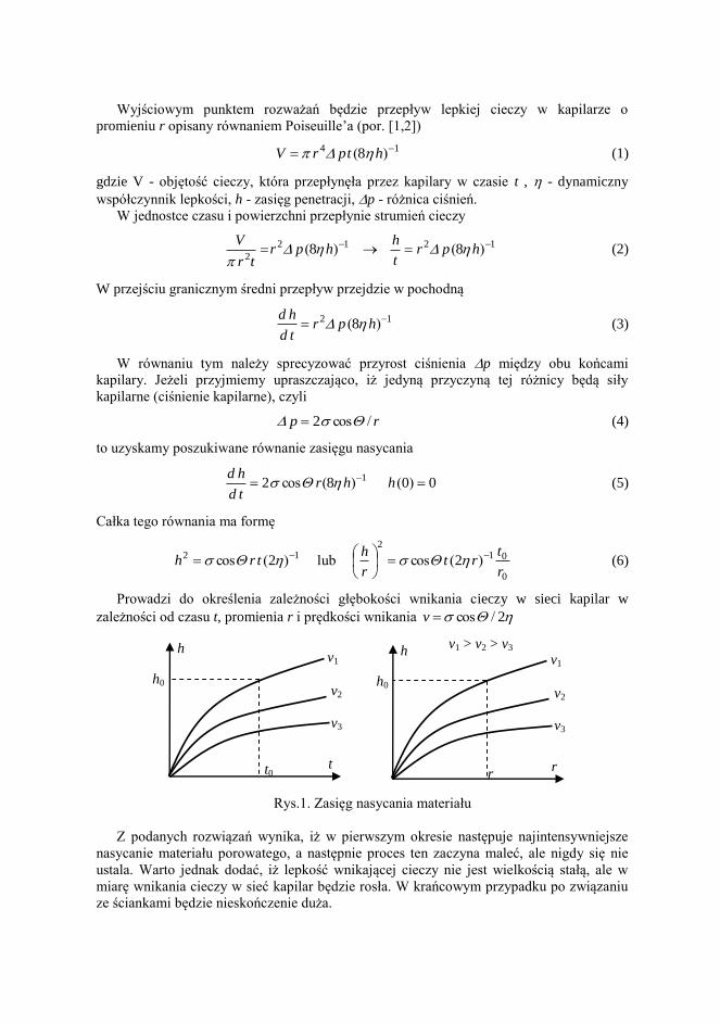
Wyjściowym punktem rozważań będzie przepływ lepkiej cieczy w kapilarze o

promieniu r opisany równaniem Poiseuille’a (por. [1,2])

14 8 )( htprV (1)

gdzie V - objętość cieczy, która przepłynęła przez kapilary w czasie t , - dynamiczny

współczynnik lepkości, h - zasięg penetracji, p - różnica ciśnień.

W jednostce czasu i powierzchni przepłynie strumień cieczy

1212

288 )( )( hpr

t

hhpr

tr

V

(2)

W przejściu granicznym średni przepływ przejdzie w pochodną

12 8 )( hprtd

hd (3)

W równaniu tym należy sprecyzować przyrost ciśnienia p między obu końcami

kapilary. Jeżeli przyjmiemy upraszczająco, iż jedyną przyczyną tej różnicy będą siły

kapilarne (ciśnienie kapilarne), czyli

rp /cos 2 (4)

to uzyskamy poszukiwane równanie zasięgu nasycania

0082 1 )( )(cos hhrtd

hd (5)

Całka tego równania ma formę

0

012

12 22r

trt

r

htrh

)(cos lub )(cos (6)

Prowadzi do określenia zależności głębokości wnikania cieczy w sieci kapilar w

zależności od czasu t, promienia r i prędkości wnikania 2/cosv

Rys.1. Zasięg nasycania materiału

Z podanych rozwiązań wynika, iż w pierwszym okresie następuje najintensywniejsze

nasycanie materiału porowatego, a następnie proces ten zaczyna maleć, ale nigdy się nie

ustala. Warto jednak dodać, iż lepkość wnikającej cieczy nie jest wielkością stałą, ale w

miarę wnikania cieczy w sieć kapilar będzie rosła. W krańcowym przypadku po związaniu

ze ściankami będzie nieskończenie duża.

h

t

v1

v3

v2

h0

t0

h

r

v1

v3

v2

v1 > v2 > v3

h0

r

3. Wiązanie cieczy w sieci kapilar

Podane poprzednio rozważania dotyczyły idealnego przypadku, kiedy to przepływająca

kapilarami ciecz posiada stałą lepkość dynamiczną 0. Tymczasem w wyniku

oddziaływania z otoczeniem i ściankami kapilar dochodzi do zmiany lepkości, tak, iż po

pewnym czasie krytycznym ustanie przepływ.

Proces ten w najprostszym przypadku opisują zależności

101

0

)(t (7)

gdzie parametr strukturalny spełnia równanie ewolucji

00 )( , ),...,,,(

prTftd

d 10 )(t (8)

W najprostszym ujęciu, kiedy znamy dla danej temperatury, średnicę kapilar i czas

wiązania tk migrującej cieczy z ścianką kapilary to można przyjąć potęgową postać funkcji n

kt

trTAt

),()( , gdzie ),( rTA , tk i n należy wyznaczyć z eksperymentu.

Wyznaczenie zmian parametru strukturalnego )(t jest odrębnym zadaniem, ponieważ

jest to wielkość materiałowa uzależniona głównie od własności powierzchniowych ścianek

kapilary i temperatury. Parametr ten opisuje bowiem przemiany fazowe zachodzące w

kontakcie powierzchni kapilary z medium nasączającym.

Podstawiając zmienną wartość współczynnika lepkości określoną równaniem (7) do

równania (5) otrzymamy

))(()(cos thrtd

hd 14 1

0 , 00 )(h (9)

stąd

dttrhdh ))(()(cos 110

4 (10)

lub w formie bezwymiarowej

t

kk

tdttr

r

h

0

10

21

2 ))(()(cos (11)

0

Otrzymana zależność pozwala na łączne analizowanie procesu nasycania kapilar przez

penetrujący przepływ lepkiej cieczy oraz procesu wiązania przepływającej cieczy z

ściankami kapilar. Procesy te działają przeciwnie, tak, iż w chwili krytycznej następuje stan

równowagowy z zaniknięciem przepływu. Czas ten też limituje głębokość wnikania cieczy

nasączającej w materiał.

Natomiast oszacowanie z nadmiarem (z góry) grubości wnikania cieczy otrzymamy

podstawiając czas krytyczny tk do równania (6).

4. Uwagi końcowe

W zabiegach konserwatorskich często występuje sytuacja, kiedy wymagamy pełnej

penetracji renomowanego elementu. W tym przypadku grubość penetracji jest określona,

natomiast do wyznaczanie pozostaje współczynnik lepkości rozpuszczalnika, który limituje

zasięg penetracji. Wyznaczenie tych parametrów należy dokonać na podstawie zadania

odwrotnego do równań (9) w powiązaniu z eksperymentem.

Drugim, odmiennym przypadkiem jest wnikanie cieczy konserwującej w cienką

powłokę farby. W tym zadaniu istotne jest wzmocnienie samej powłoki oraz związanie jej z

podłożem. Problemy technologiczne w obu przypadkach są odmienne, ale model procesu

pozostaje bez zmian.

Literatura

[1] AKSIELRUD G.A., KYSIAŃSKI M.: Ekstrakcja w układzie ciało stałe - ciecz, WNT

Warszawa 1978

[2] POHORECKI R., WROŃSKI S.: Kinetyka i termodynamika procesów inżynierii

chemicznej, WNT Warszawa 1988

SURFACE SATURATION KINETICS

Summary In the work the process of saturation of a surface with coating ensuring protection

against external factors will be analyzed. This situation can occur during renovation of

paintings and spraying of protective hydrophobic coatings.



STATICKÁ ANALÝZA ZDĚNÝCH KONSTRUKCÍ

KARLOVA MOSTU V PRAZE

Alois MATERNA, Jiří BROŢOVSKÝ

VŠB – Technická Univerzita Ostrava, Česká republika

1. Úvod

Jedním z důleţitých kroků při přípravě projektu rekonstrukce jakékoli historické

inţenýrské stavby je i analýza jejího statického působení, která musí vycházet

z vlastností materiálů získaných podrobným průzkumem. Jako součást řešení

grantového projektu 103/02/0990 „Výzkum vlivu nesilových účinků a agresivního

prostředí na stárnutí historických staveb se zvláštním zaměřením na Karlův most v

Praze“ vedeného prof. Witzanym z ČVUT v Praze jsou na Fakultě stavební VŠB-TU

Ostrava prováděny numerické simulace statického působení Karlova mostu v Praze.

Jeden z ověřovaných výpočtových modelů je diskutován v příspěvku.

Karlův most je nejstarším dochovaným praţským mostem. Spojuje praţské čtvrti

Malou Stranu a Staré Město. Je dlouhý 516 m, má šířku 10 m a je postaven na šestnácti

pilířích. Nahradil původní Juditin most, zničený při povodni v roce 1342. Most nechal

vybudovat v roce 1357 Karel IV. Most je po obou stranách opatřen obrannými věţemi

- Malostranskou a Staroměstskou. Během své existence byl most několikrát poškozen

povodněmi i válečnými událostmi. Poslední generální oprava mostu proběhla v letech

1965-1978. Opravou měla odstranit příčiny poruch - rozevírání mostu mělo být

zastaveno soustavou kotev, nad vyrovnávacími vrstvami z opukové rovnaniny byla

zhotovena ţelezobetonová deska o tloušťce 200 mm se sítí táhel, nová izolace měla

omezit účinky teplotních změn a pronikání vody. Na vnějším líci zdiva byly vyměněny

všechny poškozené pískovcové kvádry. Asfaltový povrch mostovky nahradily štípané

pásky ţuly. Most je v současnosti vyhrazen pouze pro pěší.

V příspěvku jsou prezentovány výsledky numerické analýzy vybraného pole.

Řešeny byly účinky změny teploty a pootočení mostního pilíře. Výpočty byly

provedeny programovým systémem ANSYS [1].

2.Výpočtový model

Nosná konstrukce mostu je modelována pomocí osmiuzlových prostorových

konečných prvků SOLID45. Pomocí stejných prvků jsou modelovány také výplňové

materiály v konstrukci. Betonová deska provedená při poslední rekonstrukci je

modelována pomocí skořepinových prvků SHELL63.

Analyzován byl vybraný oblouk mostu. Byla uváţena řada zatěţovacích stavů, v

příspěvku jsou pro ilustraci uvedeny dva – kombinace pootočení pilíře a zatíţení

vlastní tíhou konstrukce, dále byl analyzován vliv účinku teplotních změn

ţelezobetonové desky účinkem změny teploty na nosnou konstrukci.

Analýza účinku roztaţení betonové desky na nosnou konstrukci mostu byla řešena

jako samostatný zatěţovací stav, aby bylo moţné snadněji identifikovat vliv tohoto

zatíţení na stav napjatosti a na deformaci konstrukce. Výpočet byl proveden jako jedna

z analýz, jejichţ cílem je podrobněji definovat účinky tohoto relativně nedávno

zabudovaného prvku na zbytek konstrukce.

Ve stávající etapě prací byly prováděny analýzy za předpokladu lineárně pruţného

chování pouţitých materiálů. Byly pouţity tzv. homogenizované vlastnosti materiálu,

které byly získány z dostupné literatury a z výsledků dosavadních průzkumných prací

na Karlově mostě [2].

Obr. 1 Výpočtový model

Fig 1 Computational Model

2. Výsledky

Při provedených analýzách byly stanoveny účinky jednoho z moţných způsobů

působení betonové desky na historickou konstrukci Karlova mostu. Získané výsledky

jsou zdokumentovány v grafické části příspěvku (viz obr. 2 - 5). Obr. 2 a obr. 3

znázorňují průběh celkových a horizontálních posunutí vlivem změny teploty desky

20oC.

Obr. 2 Celkové deformace – nosná konstrukce

Fig. 2 Total displacement usum

Obr. 3 Přetvoření nosné konstrukce

Fig. 3 Horizontal deflections

Na obr. 4 a 5 je uveden průběh hlavních napětí vlivem změny teploty desky o 20oC.

Obr. 4 První hlavní napětí

Fig. 4 First principal stress

Obr. 5 První hlavní napětí

Fig. 5 First principal stress

Na obr. 6 a 7 jsou zobrazena posunutí způsobená pootočením pilíře při současném

účinku vlastní tíhy.

Obr. 6 Celkové deformace

Fig. 6 Total displacement

Obr. 7 Celkové deformace

Fig. 7 Total displacement

Závěr

Získané výsledky dále rozšiřují dostupné informace o statickém působení mostu.

Dosavadní analýzy však nelze označit za úplné nebo dokončené. Vzhledem k

charakteru, době existence a historii (včetně řady poruch, havárií a provedených, více

nebo méně zdařilých, rekonstrukcí) této významné konstrukce existuje stále mnoho

aspektů, které musí být posouzeny a vyhodnoceny. Velký význam pro další numerické

analýzy má také postupné získávání upřesněných údajů o geometrii, vlastnostech

pouţitých konstrukčních materiálů a měření deformací a teplot konstrukce, které

probíhá v rámci řešeného grantového projektu.

Práce byly prováděny s podporou grantového projektu Grantové agentury České republiky

103/02/0990 „Výzkum vlivu nesilových účinků a agresivního prostředí na stárnutí historických

staveb se zvláštním zaměřením na Karlův most v Praze“.

Literatura

[1] Dokumentace programového systému ANSYS verze 6.1, ANSYS Inc., 2001

[2] Witzany J., Čejka T., Zemánek J.: Chemická a biochemická degradace Karlova mostu,

analýza odolnosti a bezpečnosti kamenné mostní konstrukce při povodni, průzkum

základového zdiva a základů mostních pilířů, Stavební obzor, Praha, 2003

STATICAL ANALYSIS OF THE MASONRY STRUCTURES

OF THE CHARLES BRIDGE IN PRAGUE

Summary In the paper the results of numerical analyses of the models of the Charles Bridge are

presented. The problem of temperature changes and behaviour of reinforced concrete

plate build in during the last reconstruction and settlement of the pier are studied.



O FENOMENOLOGICZNYM OPISIE

PROBLEMÓW FIZYKI BUDOWLI

Jerzy WYRWAŁ


1. Wprowadzenie

Przy rozwiązywaniu wielu praktycznych zagadnień fizyki budowli posługujemy się

pojęciami, prawami i metodami fenomenologicznego opisu zjawisk fizycznych, którymi

rządzą prawa przyrody. Według [1] prawa te są: uniwersalne, absolutne, ponadczasowe i

wieczne oraz wszechwładne. Prawa przyrody powodują, że materia i energia same z siebie

organizują się w złożone formy i struktury, które staramy się opisać przy pomocy teorii

naukowych.

Według [2], teoria naukowa jest modelem istniejącego zjawiska oraz zbiorem reguł

wiążących wielkości tego modelu z obserwacjami, jakie możemy wykonać. Warto

zauważyć, że każda teoria naukowa pozostaje zawsze hipotezą, której nie potrafimy nigdy

udowodnić [2].

Chcąc opisać zjawisko będące przedmiotem naszego zainteresowania, musimy wziąć

pod uwagę [3]: przedmiot badań, narzędzia badawcze, formalizm matematyczny, nasz

zmysł obserwacyjny oraz umysł. Opis taki powinien uwzględniać najważniejsze

charakterystyki badanego zjawiska i w jego ramach, przy pomocy ogólnych praw przyrody,

możemy wyprowadzić relacje występujące między tymi charakterystykami.

2. Aspekty opisu fenomenologicznego

Opisywane przez fizykę budowli zjawiska zachodzą w makroskopowych obiektach

materialnych dostępnych naszemu poznaniu przy pomocy zmysłów. Właściwości takich

obiektów określają charakterystyki mikrocząstek, a wszystkie obserwowane zjawiska oraz

prawa nimi rządzące są konsekwencją ruchu i oddziaływań tych cząstek [2]. Właściwości

obiektów materialnych i zjawisk w nich zachodzących możemy opisać z różnym stopniem

dokładności. W fizyce budowli najczęściej korzystamy z opracowanego jeszcze w XIX

wieku opisu fenomenologicznego. Opis ten, bazujący na danych eksperymentalnych

i nadający się dobrze do wielu zastosowań praktycznych, wymaga: analizy danych

doświadczalnych, ich uogólnienia oraz zbudowania odpowiedniego modelu

matematycznego badanego zjawiska.

Poglądową interpretację wielu praw i pojęć oraz głębsze ich zrozumienie umożliwia

opis statystyczny. Jednak z uwagi na fakt, iż jest on skomplikowany i obarczony zbyt

licznymi hipotezami, to nie może w pełni zastąpić ujęcia fenomenologicznego [5].

Ponieważ fenomenologiczny opis zjawisk korzysta z wybranych praw fizyki (zasad

termodynamiki) oraz z formalizmu matematycznego i wyników badań doświadczalnych, to

warto omówić krótko role jakie w nim odgrywają: termodynamika, matematyka

i eksperyment. Być może pozwoli to spojrzeć z nieco ogólniejszej i szerszej perspektywy

na wiele problemów podstawowych i praktycznych fizyki budowli.

2.1. Aspekt termodynamiczny

Termodynamika jest dyscypliną naukową, którą wykorzystujemy do badania przemian

energetycznych zachodzących w makroskopowych ośrodkach materialnych. Podstawą

termodynamiki są obserwacje rzeczywistości fizycznej oraz nagromadzone fakty

doświadczalne. Umożliwiły one sformułowanie pewnych ogólnych praw, a mianowicie

zasady zachowania energii i zasady wzrostu entropii.

Chociaż procesy energetyczne zachodzące w materii – spowodowane ruchem atomów

i molekuł – są bardzo skomplikowane, to w ujęciu fenomenologicznym nie musimy (na

szczęście) zajmować się opisem ruchu poszczególnych atomów i cząsteczek, gdyż

interesują nas zmiany makroskopowych wielkości fizycznych, takich jak ciśnienie,

temperatura, naprężenie itp. Analiza zachowania i degradacji energii podczas wszelkiego

rodzaju procesów fizycznych, chemicznych i biologicznych (zwanych ogólnie procesami

termodynamicznymi) jest podstawowym zadaniem termodynamiki.

We wszystkich rzeczywistych, czyli nieodwracalnych procesach termodynamicznych

przekształcane są różne postacie energii, przy czym tylko część energii początkowej jest

użyteczna i uporządkowana natomiast jej pozostała część zostaje rozproszona

(bezpowrotnie stracona) w postaci ciepła. Wydzielanie się ciepła wskutek dyssypacji

(rozpraszania) energii, może niekiedy stanowić poważny problem. Dlatego też, w

pierwszym okresie rozwoju termodynamiki szukano sposobu pokonania nieodwracalności

procesów, a tym samym strat energii. Zakładano, że jeżeli proces termodynamiczny

przebiega nieskończenie powoli – czyli jest procesem quasi-równowagowym – to nie

występuje w nim rozpraszanie energii. Na takim ujęciu bazuje termostatyka

(termodynamika równowagowa albo termodynamika procesów odwracalnych), która

wyklucza jakiekolwiek zmiany badanego procesu w czasie.

Rozwój termostatyki był w głównej mierze zasługą GIBBSA, którego idee pozwalają

zrozumieć, kiedy ewolucja (zmiana ukierunkowana) układu termodynamicznego dobiega

kresu. Gdy układ izolowany (obiekt fizyczny wyodrębniony rzeczywiście lub myślowo

z otoczenia i nie wymieniający z nim ani materii, ani energii) znajduje się w stanie

równowagi, to ten końcowy stan, w jakim znalazł się układ w drodze ewolucji, opisuje

jedna wielkość termodynamiczna, a mianowicie entropia – wielkość wprowadzona przez

CLAUSIUSA. W takim stanie entropia osiąga maksymalną możliwą wartość.

Badając zachowanie układów zamkniętych (wymieniających z otoczeniem tylko

energię) oraz otwartych (wymieniających z otoczeniem zarówno energię, jak i materię)

i poszukując stanu maksymalnej entropii, musimy wziąć pod uwagę również wpływ

otoczenia. W takim przypadku możemy skorzystać z innej wielkości termodynamicznej,

czyli energii swobodnej, która odgrywa zasadniczą rolę w fizyce i chemii układów

znajdujących się w równowadze termodynamicznej.

Entropia i energia swobodna są potencjałami termodynamicznymi, co oznacza, że ich

wartości ekstremalne – minimum energii swobodnej i maksimum entropii – określają stan

równowagi. A więc ostateczny stan równowagi termodynamicznej układu zależy od

osiągnięcia maksymalnej wartości entropii lub minimalnej – energii swobodnej, nie zaś od

stanu początkowego.

Termostatyka, mimo wspomnianych wyżej wad, może stanowić wygodne narzędzie

do badania właściwości takich procesów termodynamicznych, których zależność od czasu

możemy pominąć. Musimy jednak pamiętać o tym, iż dostarcza ona mało informacji

niezbędnych do analizy rzeczywistych procesów, które z natury rzeczy są nieodwracalne

[7].

Więcej informacji na temat procesów nieodwracalnych dostarcza nam termodynamika

nierównowagowa. Dzieli się ona w naturalny sposób na dwie części: termodynamikę

liniową oraz termodynamikę nieliniową.

Liniowa termodynamika nierównowagowa bada ewolucję procesów

nierównowagowych w bliskim otoczeniu stanu równowagi. W obszarze tym obowiązują

prawa bazujące na założeniu ONSAGERA, iż w przypadku takich procesów istnieje prosta

proporcjonalność między skutkiem (zwanym przepływem termodynamicznym)

a wywołującą go przyczyną (zwaną bodźcem termodynamicznym). Należy zaznaczyć, że

wielkości te nie są bliżej sprecyzowane i jest to podstawowa wada takiego ujęcia [8].

Z kolei termodynamika nieliniowa, badająca procesy termodynamiczne z dala od

stanów równowagi, umożliwiła analizę zagadnień stabilności w procesach

nieodwracalnych. Zaowocowało to sformułowaniem przez PRIGOGINE’A koncepcji struktur

dyssypatywnych [9], czyli uporządkowanych struktur, w tworzeniu których konstruktywną

rolę odgrywają procesy rozpraszania energii. Struktury takie, nie spotykane w warunkach

równowagi termodynamicznej, mogą samorzutnie powstawać w trakcie procesów

nieodwracalnych w rodzaju przewodzenia ciepła czy też dyfuzji.

Jedna z nieklasycznych gałęzi termodynamiki, zwana termodynamiką kontinuum

materialnego [10], zajmuje się procesami w obiektach materialnych, które traktowane są

jako zbiór oddziałujących ze sobą układów termodynamicznych. Najmniejszym takim

układem jest cząstka materialna, traktowana jako układ jednorodny, którego stan

termodynamiczny opisują wielkości fizyczne, zwane parametrami termodynamicznymi.

Zgodnie z termodynamiką kontinuum, rozpraszanie energii ujmuje nierówność wzrostu

entropii [8], która w powiązaniu z bilansami: masy, pędu, momentu pędu i energii określa

klasę procesów dopuszczalnych w kontinuum materialnym.

Ponieważ duża liczba procesów makroskopowych przebiega powoli (w porównaniu

z procesami na poziomie molekularnym), to możemy z zadowalającym przybliżeniem

założyć, iż cząstki materialne znajdują się w stanie lokalnej równowagi termodynamicznej,

lub niewiele od tego stanu odbiegają. W takim przypadku możemy jednoznacznie

zdefiniować wszystkie potencjały termodynamiczne. Powinniśmy jednak pamiętać o tym,

że takie postępowanie jest ograniczone do procesów powolnych i nie wolno go

bezkrytycznie uogólniać na przypadki procesów szybkich.

Z kolei w termodynamice racjonalnej [8], odnoszącej się do szerokiej klasy procesów

nieodwracalnych i nierównowagowych, zakłada się, że wszystkie parametry

termodynamiczne, takie jak entropia, temperatura itp., są dobrze określone w przypadku

dowolnego procesu termodynamicznego1, zaś dyssypacja energii ujmowana jest przez

nierówność CLAUSIUSA-DUHEMA. Z innych założeń szczegółowych, dotyczących np.

istnienia potencjałów termodynamicznych oraz postaci wyrażenia określającego produkcję

entropii, korzysta się tylko w przypadkach szczególnych. Należy podkreślić, że

konsekwencje takiego ujęcia są zasadniczej natury i skutkują brakiem istotnych ograniczeń

(poza nierównością CLAUSIUSA-DUHEMA) na postacie związków między parametrami

termodynamicznymi, które mogą mieć bardzo ogólną postać, na przykład funkcjonałów,

relacji różniczkowych itp. [10].

Oba powyższe założenia podlegają ciągłej weryfikacji i uściślaniu [8]. Dotyczy to

w pierwszym rzędzie temperatury i entropii. I tak, założenie o lokalnej równowadze

termodynamicznej pozwala tym wielkościom odzyskać ich sens fizyczny (wielu badaczy

ma wątpliwości, czy wielkości te mogą być określone, czyli zmierzone, poza stanem

równowagi termodynamicznej). W przypadku nierówności CLAUSIUSA-DUHEMA proponuje

się, aby zastąpić ją ogólniejszą nierównością CLAUSIUSA-DUHEMA-MÜLLERA [11].

Chociaż racjonalna termodynamika kontinuum materialnego znajduje się w stanie

ciągłego rozwoju i ma niewątpliwe osiągnięcia, to boryka się ona z wieloma trudnościami

pojęciowymi i interpretacyjnymi. Wydaje się więc, że w odróżnieniu od termodynamiki

klasycznej daleka jest ona od stanu zamkniętej teorii [12].

2.2. Aspekt matematyczny

Według [3], istotą nauki jest odkrywanie istniejących w badanych zjawiskach struktur

i regularności oraz wynajdowanie sposobów opisu danych doświadczalnych. Wiedzę

o naturze zjawiska uzyskujemy na dwa odrębne sposoby. Pierwszym z nich jest

bezpośrednia obserwacja, zaś drugim logiczne rozumowanie przy wykorzystaniu naszego

umysłu. Przy pomocy tych sposobów możemy zbudować model matematyczny badanego

zjawiska. Chociaż taki model nie jest tym, co naprawdę obserwujemy, to dostarcza on

ogólnej wiedzy o badanym zjawisku, a więc możemy je poznać przy pomocy odpowiednio

dobranych eksperymentów, abstrakcyjnego rozumowania i racjonalnych procedur

matematycznych.

Badanie wielu podstawowych problemów fizyki budowli polega na budowaniu

pewnych abstrakcyjnych struktur (mniej lub bardziej skomplikowanych), które nazywamy

ich matematycznymi modelami. Warto zauważyć, że przez konstruowanie modelu

matematycznego możemy lepiej i głębiej zrozumieć badane zjawisko. Pomiędzy

obserwowanymi zjawiskami a ich matematycznymi modelami musi występować

sprzężenie; model matematyczny powinien właściwie przewidywać skutki zjawisk,

natomiast obserwacja lub doświadczenie powinny te skutki potwierdzać.

Obiekty materialne, będące tworami przyrody lub dziełami rąk ludzkich, są zbiorami

cząstek i pól fizycznych, w których zachodzą procesy energetyczne [1]. Zarówno budowę

wewnętrzną takich obiektów, jak i naturę procesów w nich zachodzących możemy

opisywać przy wykorzystaniu praw, wyrażonych za pomocą odpowiednich równań

matematycznych. Ale matematyka pozwala nie tylko opisać zjawisko, lecz również

przewidzieć jego przebieg. Wynika to z faktu, że matematyka zajmuje się przede

wszystkim badaniem relacji (czyli związków) pomiędzy obiektami (strukturami)

matematycznymi, których natura ma znaczenie drugorzędne. Okazuje się przy tym, iż

pewne struktury matematyczne dobrze opisują naturę zjawisk fizycznych. Przez zagłębianie

1 Entropia i temperatura są tu pojęciami pierwotnymi, co oznacza, że wielkości tych nie

definiujemy oraz nie podajemy sposobu ich mierzenia [13].

takich struktur lepiej poznajemy same zjawiska. By się przekonać o tym, czy struktura taka

jest właściwie dobrana, musimy wykonać odpowiednie eksperymenty potwierdzające (bądź

nie) to, co o istocie zjawiska z niej wyczytaliśmy. Zatem metoda badawcza fizyki budowli

sprowadza się do zastępczej analizy struktur matematycznych, zaś informacje uzyskane na

tej drodze musi potwierdzić eksperyment.

Korzystając z aparatu badawczego matematyki powinniśmy pamiętać o tym, aby nie

zaniedbać zasadniczych różnic między operacjami matematycznymi a badanymi

wielkościami i zjawiskami. Modele matematyczne są niekiedy tak efektowne i skuteczne, iż

moglibyśmy uwierzyć, że one same są obiektywną rzeczywistością. A przecież świat

badanych zjawisk nie jest równie ścisły jak jego matematyczny model. Wielkości

matematyczne są zawsze dokładne, zaś operacje matematyczne mogą być albo prawdziwe,

albo fałszywe; natomiast wyniki badań eksperymentalnych nie są już tak jednoznaczne. To,

co możemy obserwować w pracy badawczej, to nie są równania matematyczne, ale

zjawiska fizyczne i właśnie ich badanie dostarcza nam niezbitych faktów, na których

możemy opierać interpretację teorii naukowych [14]. Zatem model matematyczny opisuje

zjawisko fizyczne tylko wtedy, gdy zostanie zweryfikowany doświadczalnie.

2.3. Aspekt eksperymentalny

Mówiąc o roli eksperymentu musimy uzmysłowić sobie fakt, iż prowadząc badania

doświadczalne musimy ograniczyć swoje zainteresowania tylko do tych wielkości, które

możemy zmierzyć. Wyniki przeprowadzonych pomiarów służą do określenia zbioru

wyjściowych założeń, na bazie których, w drodze matematycznej dedukcji, możemy

zbudować wiele różnych modeli matematycznych danego zjawiska fizycznego. Porównując

te teoretyczne modele z wynikami eksperymentów (czyli z wynikami pomiarów)

odrzucamy wszystkie te, których doświadczenie nie potwierdza [3].

Należy podkreślić, iż między teorią a eksperymentem zachodzi sprzężenie zwrotne:

instrumenty pomiarowe budujemy przy wykorzystaniu teorii, zaś teorię tworzymy opierając

się na wynikach doświadczeń wykonanych przy pomocy tych instrumentów. Stąd

wszystko, co wykracza poza przedstawiony wyżej sposób postępowania, znajduje się poza

obszarem właściwej i skutecznej metody badawczej. To, że potrafimy badać świat

metodami eksperymentalnymi jest bezpośrednim następstwem faktu posiadania przez nas

świadomości refleksyjnej [3].

Według [15] metoda doświadczalna jest prawdziwą sztuką, a to oznacza, że opiera się

ona na szczególnych umiejętnościach badacza, a nie na ogólnych prawach i procedurach

badawczych. Z uwagi na tę szczególną jej cechę, nie gwarantuje ona nigdy sukcesu.

Zawsze istnieje niebezpieczeństwo, że wyciągnięte z badań wnioski są mylne lub też

banalne. Żadna metodologiczna i racjonalna procedura badawcza nie usunie ryzyka

wyciągnięcia fałszywych wniosków z przeprowadzonych rozważań i analiz. Metoda

doświadczalna jest sztuką właściwego postawienia badanego problemu oraz prześledzenia

wszystkich konsekwencji wiążących się z takim wyborem, a także przewidywania

wszelkich procedur eksperymentalnych, spośród których musimy następnie wybrać tę,

która wydają się nam najodpowiedniejsze jako podstawa jednoznacznego sprawdzenia

przewidywań teorii.

3. Podsumowanie

Zjawiska fizyczne zachodzące obiektach materialnych będących przedmiotem badań

fizyki budowli (np. przenoszenie masy i energii) są konsekwencją ruchu i oddziaływań

mikroskopijnych cząstek materialnych (np. atomów i molekuł). Właściwości takich

obiektów i zjawisk w nich zachodzących możemy opisać przy wykorzystaniu opisu

fenomenologicznego, który wymaga analizy danych eksperymentalnych, ich uogólnienia i

zbudowania na tej podstawie modelu matematycznego zjawiska. Podstawową rolę przy

formułowaniu problemów fizyki budowli przy wykorzystaniu opisu fenomenologicznego

odgrywają: termodynamika, matematyka i eksperyment.

Literatura

[1] Davies P.: Plan Stwórcy. Wydawnictwo ZNAK, Kraków 1996.

[2] Hawking S.: Krótka historia czasu. Od wielkiego wybuchu do czarnych dziur.

Wydawnictwo „Alfa”, Warszawa 1990.

[3] Heller M.: Usprawiedliwianie wszechświata. Wydawnictwo ZNAK, Kraków 1995.

[4] Feynman R.: Charakter praw fizycznych. Prószyński i S-ka, Warszawa 2000.

[5] Włodarczyk E.: Wstęp do mechaniki wybuchu. Wydawnictwo Naukowe PWN,

Warszawa 1994.

[6] Ho-Kim Q., Kumar N., Lam Ch-S.: Zaproszenie do fizyki współczesnej.

Stowarzyszenie Symetria i Własności Strukturalne, Poznań 1995.

[7] Korzeniewski B.: Trzy ewolucje. Małopolska Oficyna Wydawnicza KORONA,

Kraków 1997.

[8] Truesdell C.: Rational Thermodynamics. Springer-Verlag, New York 1984.

[9] Nicolis G. Prigogine I.: Self-Organization in Nonequilibrium Systems. From

Dissipative Structures to Order through Fluctuations. Willey&Sons, New York 1977.

[10] Rymarz Cz.: Mechanika ośrodków ciągłych. Wydawnictwo Naukowe PWN,

Warszawa 1993.

[11] Müller I. : Thermodynamics. Pitman, London 1985.

[12] Wilmański K.: Termodynamika fenomenologiczna. Podstawy mechaniki (ZORSKI H.

red.), Wydawnictwo Naukowe PWN, Warszawa 1985.

[13] Muschik W., Papenfuss C., Echrentraut H.: A sketch of continuum thermodynamics.

J. Non-Newtonian Fluid Mech., 96, 2001, 255-290.

[14] Speyer E.: Spadkobiercy Newtona. Wydawnictwo Amber, Warszawa 1997.

[15] Prigogine I., Stengers I.: Z chaosu ku porządkowi. Państwowy Instytut Wydawniczy,

Warszawa 1990.

ON THE PHENOMENOLOGICAL DESCRIPTION

OF THE BUILDING PHYSICS PROBLEMS

Summary

In the paper the general considerations applied to phenomenological description of

research problems of building physics are presented. This description basis on experimental

results and is suitable for many practical applications. It also demands an experimental data

analysis together with its generalisation and building a mathematical model of investigated

phenomenon. There is also compared phenomenological description with statistical one.

Fundamental aspects of phenomenological description, such as: thermodynamical,

mathematical and physical one, are discussed.

With the partial support of the Commission of the European Communities under the

FP5, contract No. G1MA-CT-2002-04058 (CESTI)

ROCZNIKI INŻYNIERII BUDOWLANEJ - ZESZYT 3/2004


PORÓWNANIE ENERGII W TEORII UŚREDNIANIA

WAGOWEGO

Jan KUBIK


1. Wprowadzenie

Intensywnie rozwijane ostatnio opisy procesów termomechanicznych na poziomie

mikroskopowym zakładają zarówno zasadność uśrednień parametrów określających proces,

czyli przejścia z poziomu mikro na makro, jak i procesu odwrotnego (lokalizacji), który

pozwoli przejść z rozwiązania makroskopowego na mikroskopowe. Dodatkowo zakłada się,

iż na obu poziomach obowiązuje ten sam typ równań mechanicznych procesu. Przy analizie

przejść z poziomu mikro na makroskopowych opisów istotne są oszacowania parametrów

określających te transformacje. Jedną z możliwości daje postulat równości całkowitej

energii w obu opisach. W pracy porównuje się energię na obu poziomach opisu uzyskując

kryterium energetycznej równoważności obu opisów.

2. Metoda wagowego uśredniania

Zakładamy, że na poziomie mezo- wielkość polowa Aij zależy od zmiennej yj i czasu t, a

na poziomie makroskopowym po uśrednieniu występuje wielkość wygładzona <Aij>, który z

polem Aij(yk,t) łączy formuła uśredniania

mAdyxymtyAtxA ij

B

kkkkijkij )(),(),( (1)

gdzie waga m jest ciągłą i parzystą funkcją o zwartym nośniku w B. Funkcja ta może

fizycznie opisywać np. proces zanikania oddziaływań. Wzór (1) określa również

transformację pól z poziomu mezo- na makroskopowy m: Aij(yi,t) <Aij(xi,t)>.

W dalszych rozważaniach przydatne będą również wzory transformacyjne dla

pochodnej przestrzennej oraz czasowej. Założymy również, iż w obszarze uśredniania

znajdują się dwa składniki, tak, że pole Aij przechodzi w ijA i

ijA .

Pochodna przestrzenna wyraża się wówczas relacją (por.[1, 2])

ijkijkC

kkkijijijkk

ijKA

xdyxymnAAmA

xm

y

A

(2)

Podobnie pochodna czasowa wyraża się zależnością

ijij

C

kkkkkijijijij

LAt

dyxymvnAAmAt

mt

A

(3)

W podanych wzorach symbolami kvnC i, oznaczono kolejno powierzchnię

międzyfazową /, wektor normalnej do tej powierzchni oraz prędkości powierzchni

rozdziału faz.

3. Zadania brzegowe

Zadanie początkowo-brzegowe w opisie mikroskopowym ujmuje układ równań

ruchu dt

dvF

y

ii

j

ij

(4)

geometrycznych i

i

j

iij

y

v

y

vd

2 (5)

warunki brzegowe w naprężeniach vPn iA

jij

(6)

i przemieszczeniach iAi uu

oraz równania fizyczne. Wymienione tu pola są funkcjami

zmiennej mikroskopowej yj i czasu t.

Dokonując następnie uśrednienia wagowego zgodnie z równaniami (1)(3) otrzymamy

odpowiadające zadanie brzegowe w makroskali ),( txi .

Zachodzi

iiiiijj

ii

j

ijLv

dt

dFKm

xdt

dvFm

ym

)()( (7)

Uśrednione zadanie brzegowe w makroskali opisują równania:

ruchu

iiiiij

j

vLKFx

(8)

geometryczne

i

jj

iij v

xv

xd2 (9)

oraz warunki brzegowe iA

jij Pn

, iAi uu

(10)

W makroskali pola te są funkcjami zmiennych (xi, t).

4. Porównanie energii

Na podstawie przytoczonych poprzednio równań ruchu, warunków geometrycznych

oraz brzegowych możemy otrzymać równania bilansów energii mechanicznej w mikro- i

makroskopowym ujęciu problemu. Energie te dla tych samych obszarów można porównać z

czego wyniknie zależność całkowa łącząca oba opisy.

Mnożąc równania (4) przez vi i całkując otrzymamy

dVvvddVvFdAnvdVvdt

dvF

yV

iiijij

V V

ii

A

jiijii

iijj

)]([ (11)

stąd

V

ii

A

ii

V

dVvFdAvPdVKUdt

d )( (12)

gdzie

V

ijij

V

dUdVdt

d ,

V

ii

V

dVvdt

dvKdV

dt

d

Podobnie postąpimy z odpowiednim zadaniem w makroskali. Pomnożymy równanie (8)

przez uśrednioną prędkość <vi> i scałkujemy po tym samym obszarze co poprzednio.

Otrzymamy

V

iii

V

iiijij

V

ii

V A

jiijiiiiiijj

dVvLNdVvvddVvF

dAnvdVvvLNFx

)(

)(

(13)

stąd

V

iii

V

ii

A

ii

V

dVvLNdVvFdAvPdVKUdt

d)()( (14)

Postulując następnie, aby zmiany całkowitej energii (U+K) w opisie mikroskopowym i

uśrednionym były takie same otrzymamy zależność

V

iii

A V

iiii

A V

iiii dVvLNdVvFdAvPdVvFdAvP )( (15)

łączącą siły występujące w mikro- i makroopisie tego samego zadania brzegowego, przy

czym V oznacza tu objętość referencyjną a A jest powierzchnią tego obszaru.

5. Podsumowanie

Stosowane do opisu mikrostruktury ciał stałych metody uśredniania wagowego dają

szansę na przejście z mikroopisu na uśredniony opis makroskopowy. Przy przejściu tym

powinna pozostać niezmieniona całkowita energia układu tj. suma energii wewnętrznej i

kinetycznej. Warunek tej niezmienności jest podany w pracy.

Oznaczenia symboli

Pi – obciążenie na powierzchni układu, load on the surface of the body, [Pa]

v – prędkość składnika α , velocity of constituent α, [m/s]

ij – tensor odkształcenia, strain tensor, [-]

ij – tensor naprężenia, stress stensor, [Pa]

Fi – siła masowa, mass force, [N/m3]

, – gęstość składnika α i układu, density of constituent α and body, [kg/m3]

Literatura

[1] ŁYDŻBA D: Zastosowania metody asymptotycznej homogenizacji w mechanice

gruntów i skał, Oficyna Politechniki Wrocławskiej Monografia 23, Wrocław, 2002

[2] SUQNET P (ed.): Continuum micromechanics, CISM Courses nr 377, Springer

Verlag, 1997

Comparison of energy in the theory of weight averaging

Summary The theory of weight averaging of energy is used in the work in order to formulate the

identity, which allows us to estimate material parameters. Scalar weights are used in the

considerations, which lead to the simplest formulas of averaging. Comparison of total

energies of the mechanical system on micro and macro levels makes possible to obtain the

identity connecting both micro and macro descriptions of the system.

With the partial support of the Commission of the European Communities under the FP5, contract

No. G1MA-CT-2002-04058 (CESTI).



O wyznaczaniu współczynnika dyfuzji pary wodnej w materiale

porowatym

Andrzej MARYNOWICZ, Jerzy WYRWAŁ


1. Wprowadzenie

Z powszechnie stosowanych technik wyznaczania współczynnika dyfuzji pary

wodnej w materiałach budowlanych na szczególną uwagę zasługują dwie: całkowa [3,5]

oraz metoda bazująca na tzw. transformacji (potencjale) Kirchhoffa [1].

2. Metoda całkowa

W metodzie tej wykorzystuje się następujące równanie dyfuzji

CDt

C

. (1)

Po przemnożeniu tego równania stronami przez iloraz hx / , oraz scałkowaniu

(uśrednieniu) po grubości hx ,0 i przedziale czasu ttt, , [3,5], dostajemy

dtdxCDh

xdtdx

t

C

h

xtt

t

htt

t

h

)( )(

00

. (2)

Całkując poszczególne człony równania (2) przez części otrzymujemy:

tt

t

tt

t

tt

t

h

htt

t

h

dtChCh

DdthCDdtdxCD

h

x

dxtCttCh

xdtdx

t

C

h

x

.)]0()([)( )(

,)]()([ )(

0

00

(3)

Po podstawieniu (3) do równania (2) otrzymamy

dttDChCh

dthj

dxtCttCh

xtt

t

tt

t

h

)()]0()([1

)(

)]()([

0

. (4)

gdzie

CDvv

uj (5)

Po dalszych przekształceniach i wykorzystaniu twierdzenia o wartości średniej

otrzymamy

dxtCttCth

xhj

ChC

hD

h

)]()([

)(

)()(

00

. (6)

W wyrażeniu (6) strumień )(hj oraz stężenia )(hC i )0(C wyznaczamy przy

założeniu, że parę wodna traktujemy jako gaz doskonały [5,8], czyli

TR

p

v

vv ~ . (7)

Uwzględniając związek 1 satv pp oraz zależność (5), otrzymujemy

)0(

)0(

TR

pC

v

sat , )(

)( hTR

phC

v

sat

. (8)

We wzorach (8) wilgotność powietrza po zewnętrznej stronie próbki oraz temperaturę

przyjęto jako wartości średnie na podstawie pomiaru warunków wewnątrz komory

klimatycznej. Wilgotność po stronie wewnętrznej, przyjęto równą 95%. Strumień

dyfundującej pary wodnej, obliczono na podstawie pomiarów ubytków masy zestawu

pomiarowego typu WetCup (rys.2), korzystając z zależności

At

tmttm

At

mhj

)()(

)(

, [kg/m

2s]. (9)

Ostatecznie uwzględniając zależności (8) i (9) oraz przyjmując w miejsce koncentracji

)(tC jej wartość średnią srC , zapisujemy wzór (6) w postaci

dxtCttCth

x

At

tmttmh

p

hTRD srsr

h

sat

v )]()([

)()()()(

0

0 . (10)

3. Metoda bazująca na potencjale Kirchhoffa

W rozpatrywanym przypadku równanie (1) zapisać można jako

CCDt

C

. (11)

Chcąc uniknąć bezpośredniego wyznaczania współczynnika )(CD można wprowadzić

nową funkcję , poprzez tzw. transformację Kirchhoffa [2], w postaci

C

C

ref

ref

CdCDC . (12)

Wielkość ta ma sens fizyczny pola pod wykresem funkcji współczynnika dyfuzji

)(CD (rys. 1)

)(C C

)(CD

refC

C

Rys. 1. Sens fizyczny potencjału przepływu masy [4]

Fig. 1. Physical interpretation of mass flow potential [4]

Wielkość ref określa pewną wartość odniesienia (początkową). Różniczkowanie

C (z wykorzystaniem definicji pochodnej funkcji złożonej) da nam wyrażenie

)(CDdC

d

. (13)

Podstawiając (13) do (5) otrzymujemy

CdC

dj , (14)

Całkując (14) po grubości h (w przypadku jednowymiarowym) otrzymujemy, przy stałym

strumieniu j , relację

hh

hdxdx

ddx

dx

d

00

)0()( jj , (15)

czyli

)0()( hhj . (16)

Tak więc iloczyn strumienia i grubości określa nam różnicę potencjału. Przyjmując

jako wartość odniesienia 0)0( ref mamy dla dowolnego hx ,0

C

Cref

CdCDxx )( )( j . (17)

4. Badania doświadczalne

W badaniach wykorzystano zestaw typu WetCup (rys. 2) mierząc strumień pary przy

zadanych różnicach wilgotności po obu stronach próbki [1].

T=const, RH= 4321 ,,,

T=const, RH= 0 =95%

woda

gips

pojemnikji

komora

h

Rys. 2. Zestaw pomiarowy typu Wet Cup

Fig. 2. The Wet Cup measuring set

Mając określone strumienie dla różnych wartości ,3,2,1 ,0 ii (rys. 3), oblicza

się nachylenie otrzymanej krzywej w wybranych punktach, otrzymując w wyniku szukany

rozkład )(D [1] lub, po przeliczeniu wg (8), )(CD lub też bezpośrednio )(int D wg

(10).

Pomiarom została poddana próbka wycięta z typowej płyty gipsowo-kartonowej o

grubości 1,2cm i średnicy 8cm. Dane materiałowe zaczerpnięte zostały z pracy [7].

hi j

0 1 2 3

h 3j

0

Rys. 3. Ogólna postać rozkładu )( [1]

Fig. 3. General form of )( relation [1]

Obliczenia wykonano za pomocą programu MathCad [6], wykorzystując zestawy

danych pomiarowych dla różnych wilgotności względnych %70 ,60 ,50 ,404,3,2,1 .

Rysunek 4 przedstawia zmiany średniego współczynnika dyfuzji w funkcji wilgotności

względnej obliczone wg wyrażenia (10), przy wykorzystaniu wielomianu w postaci

2975

int 1054,31034,41078,1)( D . (18)

Średni współczynnik dyfuzji w rozpatrywanym przedziale wilgotności względnej

%7040 wyniósł smD 26int 106 .

Na rysunku 5 pokazano wyniki obliczeń potencjału Kirchhoffa . W tym

przypadku współczynnik dyfuzji obliczony został w poszczególnych przedziałach z relacji

i

iiD

, dla 3 ,2 ,1i . (19)

Rys. 4. Współczynnik dyfuzji pary wodnej )(D wg metody całkowej

Fig. 4. Water vapour diffusion coefficient according to the integral method

Średnia wartość współczynnika dyfuzji wyniosła smDpK26107 . Wielomian

aproksymujący funkcję potencjału Kirchhoffa ma postać

21197 1031055.41091,1)( . (20)

Rys. 5. Potencjał Kirchhoffa )(

Fig. 5. Kirchhoff’s potential )(

5. Podsumowanie

Z otrzymanych wyników opartych na metodzie bazującej na potencjale Kirchhoffa

wynika, że chcąc otrzymać dokładniejszy rozkład D() należy analizować większą ilość

punktów pomiarowych. Pod tym względem metoda całkowa wypada korzystniej,

pozwalając otrzymać szybciej poszukiwany rezultat. Wartości średniego współczynnika

dyfuzji otrzymane z obydwóch metod są porównywalne (różnica wynosi ok. 15%).

Spis oznaczeń

porowatość (porosity), [-]

wilgotność względna (relative humidity), [-],

D współczynnik dyfuzji pary wodnej (water vapour diffusion coefficient), [m2/s],

Dint współczynnik dyfuzji pary wodnej wg metody całkowej (water vapour diffusion

coefficient due to integral method), [m2/s],

DpK współczynnik dyfuzji pary wodnej wg potencjału Kirchhoffa (water vapour

diffusion coefficient according to Kirchhoff’s potential), [m2/s],

psat ciśnienie pary wodnej nasyconej (saturated water vapour presure), [Pa],

pv ciśnienie cząstkowe pary wodnej (partial water vapour presure), [Pa],

Rv stała gazowa pary wodnej (water wapour gas constant), [J/kgK].

Literatura

[1] Arfvidsson J., Claesson J.: Isothermal moisture flow in building materials: modelling,

measurements and calculations based on Kirchhoff’s potential. Building and

Environment, vol 35, pp. 519-636, 2000

[2] Carlslaw H, Jaeger J. C.: Conduction of heat in solids, 2nd

ed., Oxford University Press,

Oxford 1959

[3] Drhalova J, Cerny R.: Non-steady methods for determining the moisture diffusivity of

porous materials, Int. Comm. Heat Mass Transfer, vol. 25, No. 1, pp.109-116, 1998

[4] Hedenblad G.: Moisture permeability of mature concrete, cement mortar and cement

paste. Dissertation, Lund Institute of Technology, Lund 1993

[5] Kubik J.: Przepływ wilgoci w materiałach budowlanych. OW PO, Opole 2000

[6] Kucharski T.: Programowanie obliczeń inżynierskich. Wydawnictwo Politechniki

Gdańskiej, Gdańsk 2000

[7] Raznjević K.: Handbook of thermodynamic tables and charts. Hemisphere Publishing

Corporation, London 1976

[8] Wyrwał J.: Ruch wilgoci w porowatych materiałach i przegrodach budowlanych. WSI,

Studia i monografie z. 31, Opole 1989

On the determining of the water vapour diffusion coefficient in

a porous material

Summary In the presented article were discussed two methods of determination of the water

vapour diffusion coefficient in typical building material. Common techniques of its

evaluation base on long measurements, lasting often many months. Dependence of this

coefficient for many parameters, such humidity of material, its structure (porosity), or

temperature has been the additional difficulty. Also less time-consuming methods of

evaluating of this coefficient were worked out, both in non-stationary range, as in stationary

one. With regard on easy investigations two methods deserve a special attention: integral

one, and the method basing on so-called Kirchhoff's transformation (potential), which allow

us to obtain the dependence of coefficient of diffusion from any flow potential (such as

relative humidity of air, humidity of material, capillary pressure, etc).

With the partial support of the Commission of the European Community under the FP5, contact

No. G1MA-CT-2002004058 (CESTI)



VPLYV TUHOSTI PODLOŽIA NA VLASTNÉ FREKVENCIE

TENKÝCH DOSIEK

Daniela KUCHÁROVÁ

Žilinská univerzita v Žiline

1. Úvod

Tenké dosky v kontakte s podložím sú jedným z veľmi často používaných nosných

prvkov v dopravnom staviteľstve. Nachádzajú svoje uplatnenie v konštrukciách vozoviek,

ale aj v železničnom staviteľstve pri výstavbe koľaje s tzv. pevnou jazdnou dráhou. Pri

takejto konštrukcii je koľajové lôžko nahrádzané prefabrikovanými alebo monolitickými

železobetónovými doskami. Takáto konštrukcia má množstvo výhod a používa sa hlavne

v súvislosti s výstavbou vysoko rýchlostných tratí 1. Vzhľadom na malú konštrukčnú

výšku sa s úspechom používa aj v železničných tuneloch a na mostoch.

Každá stavebná konštrukcia na dopravnej ceste je vystavená evidentným dynamickým

účinkom dopravných prostriedkov, preto je potrebné okrem statickej analýzy realizovať aj

dynamickú analýzu konštrukcie ako celku a jej jednotlivých komponentov. Prvým krokom

dynamickej analýzy je stanovenie základných dynamických charakteristík, ktoré definujú

dynamickú individualitu systému, nakoľko tieto charakteristiky sú potrebné pri analýze

ohlasu konštrukcie na dané dynamické zaťaženie, analýzu rezonančných javov a následné

riešenie otázok spojených s únavou, životnosťou a spoľahlivosťou celého systému.

Charakter zaťaženia i charakter povrchu jazdnej dráhy spôsobujú, že doskové konštruk-

cie na dopravných cestách sú vystavené budiacim silám s premennou frekvenčnou sklad-

bou. Reakcia konštrukcie na takéto zaťaženie je teda závislá od spektra vlastných frekvencií

analyzovanej konštrukcie. Pokiaľ je dosková konštrukcia v kontakte s podložím, ovplyvňu-

je jej vlastné frekvencie tuhosť podložia i veľkosť spolukmitajúcej hmoty podložia.

V tomto príspevku je analyzovaný vplyv tuhosti podložia na vlastné frekvencie tenkých

dosiek pri uvažovaní Winklerovho modelu podložia.

2. Výpočtový model a realizácia výpočtov

Predmetom analýzy sú vlastné frekvencie a tvary vlastného kmitania tenkej železobetó-

novej dosky v kontakte s Winklerovým modelom podložia. Doska má pôdorysný rozmer

1300 x 1210 mm a hrúbku 200 mm. Použitý betón B40, modul pružnosti E = 3,6.1010

N.m-

2, objemová hmotnosť = 2600 kg.m

-3.

Výpočty vlastných frekvencií a tvarov vlastného kmitania sa realizovali s použitím

metódy konečných prvkov podobne ako v 2. Riešená doska je uvažovaná ako doska na

Winklerovom pružnom podklade s modulom stlačiteľnosti CW = 1,5.108 N.m

-3. Modul

stlačiteľnosti podložia bol experimentálne overovaný zaťažkávacou skúškou s použitím

kruhovej zaťažovacej dosky. Riešená oblasť bola rozdelená na 480 štvoruholníkových

konečných prvkov s 527 uzlami delenia a pokrytá prvkami troch rôznych typov. Prvých 20

vlastných frekvencií je uvedených v tab. 1. Tvary kmitania sú na obr. 1.

Tab. 1 Vlastné frekvencie dosky pri CW = 1,5.108 N.m

-3

Table 1 Natural frequencies of the plate at CW = 1,5.108 N.m

-3

Natural frequencies f(j) of the plate at CW = 1,5.108 N.m-3 in Hz

j f(j) j f(j) j f(j) j f(j)

1

2

3

4

5

75,13

77,56

78,61

168,10

198,80

6

7

8

9

10

435,6

449,9

562,0

673,7

685,4

11

12

13

14

15

815,1

979,3

1042,0

1218,0

1267,0

16

17

18

19

20

1442,0

1465,0

1609,0

1627,0

1715,0

Obr. 1 Vybrané tvary kmitania dosky pri CW = 1,5.108 N.m

-3

Fig. 1 Selected natural modes of the plate at CW = 1,5.108 N.m

-3

Okrem tejto základnej analýzy bola realizovaná aj parametrická štúdia ozrejmujúca

vplyv tuhosti podložia na hodnoty vlastných frekvencií. Hodnoty prvých dvadsiatich vlast-

ných frekvencií v závislosti od modulu stlačiteľnosti podložia CW, v intervale 1.0e5 -

1.0e10 N.m-3

, sú uvedené v tab. 2.

j =1

j = 5

j = 2

j = 4

Tab. 2 Vlastné frekvencie f(j) v závislosti od CW

Table 2 Natural frequencies f(j) versus CW

Vlastné frekvencie MŽD f(j) Hz v závislosti od tuhosti podložia CW N.m-3

j CW = 1.0e5 CW = 1.0e6 CW = 1.0e7 CW = 1.0e8 CW = 1.0e9 CW= 1.0e10

1

2

3

4

5

6

7

8

9

10

11

12

13

14

15

16

17

18

19

20

1,90

2,00

2,03

148,70

183,50

428,40

443,40

556,00

668,80

681,10

811,40

975,80

1039,00

1215,00

1265,00

1439,00

1463,00

1608,00

1625,00

1713,00

6,13

6,33

6,42

148,80

183,60

428,40

443,50

556,00

668,90

681,10

811,40

975,90

1039,00

1215,00

1265,00

1439,00

1463,00

1608,00

1625,00

1713,00

19,40

20,04

20,30

150,00

184,50

428,80

443,80

556,40

669,20

681,40

811,60

976,10

1039,00

1215,00

1265,00

1440,00

1463,00

1608,00

1625,00

1713,00

61,34

63,34

64,19

161,90

193,80

433,20

447,80

560,00

672,10

683,90

813,90

978,10

1041,00

1217,00

1266,00

1441,00

1465,00

1609,00

1626,00

1714,00

193,90

199,20

202,80

252,10

269,70

474,70

485,20

595,00

700,90

709,20

836,20

998,70

1058,00

1233,00

1282,00

1454,00

1478,00

1619,00

1638,00

1725,00

612,10

616,00

637,20

650,40

670,40

764,30

776,90

870,30

923,70

941,40

1035,00

1185,00

1218,00

1379,00

1428,00

1577,00

1601,00

1722,00

1755,00

1826,00

4. Záver

Tak ako pri statickej analýze, ktorej sa venovalo v minulosti viac autorov 1, 3, 4,

5, sa ako najvýhodnejšia metóda riešenia ukazuje metóda konečných prvkov. Analýza

vlastných frekvencií a tvarov vlastného kmitania je dôležitá pre analýzu rezonančných

javov i seizmických problémov. Výsledky poukazujú na silnú závislosť výsledkov od tu-

hostných charakteristík podložia. Veľkosť vlastných frekvencií sa s narastajúcou hodnotou

tuhosti podložia zväčšuje. Miera rastu však nie je rovnaká pre všetky vlastné frekvencie.

Najvýraznejšie je zmenou tuhosti podložia ovplyvnená hodnota najnižšej vlastnej frekven-

cie. Vlastné frekvencie sú ešte do určitej miery ovplyvňované skutočnosťou, že pri kmitaní

spolupôsobí s doskou aj určitá hmotnosť podložia. Veľkosť spolupôsobiacej hmoty podlo-

žia je možné určiť len na základe experimentálnych meraní. Z hľadiska komplexnosti posu-

dzovania konštrukcie koľaje by bolo potrebné analyzovať nielen javy prebiehajúce

v samotnej konštrukcii, ale aj javy prebiehajúce v jej podloží. Niektoré práce sledujú aj

teoretickú stránku tohoto problému 6, 7.

Tento príspevok bol vypracovaný v rámci výskumnej činnosti podporovanej vedeckou grantovou agentúrou

VEGA SR – grantová úloha č. 1/7291/20

Značky symbolov

E modul pružnosti,

objemová hmotnosť,

f(j) j-tá vlastná frekvencia,

CW modul stlačiteľnosti podložia,

j poradové číslo vlastného tvaru kmitania.

Literatúra

[1] Melcer J.: Výpočet doskových podkladov železničnej trate metódou konečných prv-

kov. Práce a štúdie Vysokej školy dopravy a spojov v Žiline, séria stavebná, zväzok 10,

1986, s.21-31.

[2] Kuchárová D.: Natural frequencies of a plate on Winkler elastic foundation. Procee-

dings of the International Conference on Dynamics of Civil Engineering Structures and

Wind Engineering, DYN-WIND´2000. Slovak Republic, Vyhne, Sitno Hotel, Sept.,

18-21, 2000, EDIS, Žilina, 2000, p.243-246.

[3] Melcer J.: Statické pôsobenie železničných dosiek. V zborníku konferencie

s medzinárodnou účasťou: Staticko–konštrukčné a stavebno–fyzikálne problémy sta-

vebných konštrukcií. Tatranská lomnica, 22. – 24.11.2000, Expo-Educ, Košice, 2000,

s.113-116.

[4] Melcer J.: Simulácia prevádzkového zaťaženia doskových podkladov koľaje.

V zborníku príspevkov XI. medzinárodnej konferencie konanej pri príležitosti 100. vý-

ročia založenia České vysoké školy technické v Brne, 18.–20.10.1999, sekcia č. 3, Sta-

vebná mechanika, VUT FAST Brno, 1999, s.157-160.

[5] Králik J.: Program MEP2DO. Riešenie pružno-plastických Mindlinových dosiek MKP

na Winkler-Pasternakovom podloží. Sb. kolokvia v Brne, Programy MKP a MHP

v ČSFR IV, ČSSM NUMEG, 1991, s.135.

[6] Králik J.: Riešenie stavu napätosti podložia pod základovou konštrukciou za uváženia

fyzikálnej a geometrickej nelinearity a jednostranných väzieb v kontakte. Zb. konfe-

rencie Využitie VT v statickom riešení základových konštrukcií. Jasná pod Chopkom,

DT ČSVTS, Košice, 1998, s.7-12.

[7] Králik J.: Problém šírenia vĺn vo vrstevnatom pružno-väzko-plastickom podloží pod

kruhovým základom. Zb. IV. vedeckej konferencie: Rozvoj výpočtových metód a apli-

kácia výsledkov výskumu pri navrhovaní stavebných konštrukcií. SvF VST, Košice,

1989, s.10-14.

INFLUENCE OF THE SUBGRADE STIFFNESS ON THE

NATURAL FREQUENCIES OF THIN PLATES

Summary Thin plates on soil are very frequently used as bearing members of the transport structures.

They are applied in road and rail structures. Transport structure is subjected to evidence

dynamic influences of moving vehicles. It is the reason for dynamic analysis of the struc-

ture. The 1st step in the dynamic analysis is the analysis of basic dynamic characteristics of

the structure. They define the dynamic individuality of the structure. Natural frequencies

and natural modes can be considered as basic dynamic characteristics of every dynamic

system. Character of the load and character of track irregularities cause that the plates are

subjected to excitation forces with variable frequency composition. Response of the struc-

ture on such excitation forces is dependant on the spectrum of natural frequencies. In the

case of plates on elastic foundation the natural frequencies of the plate are influenced by the

stiffness of subgrade. The values of natural frequencies growth with the growth value of

subgrade stiffness. The measure of growth is not the same for every natural frequency. The

lowest natural frequency is the most influenced by this factor. The natural frequencies are

influenced by the vibrating mass of subgrade too. The most suitable way how to determine

this influence is the realisation of in situ experimental measurements.



RAILWAY BRIDGE MANAGEMENT SYSTEM

IN SLOVAKIA

Josef VIČAN, Peter KOTEŠ, Jozef GOCÁL

University of Ţilina

1. Introduction

The Slovak republic should be entering the European union on 1. May 2004. The mod-

ernization of the transportation infrastructure, which consists of the highways and the rail-

way network, is the one of many conditions which should be satisfied in order to enter EU.

On the basis of this fact, the phase of the infrastructure rehabilitation of existing railways

has begun. The part of the railways is rebuilt to the high-speed railways and the rest one is

rehabilitated. Many deteriorated and damaged bridges are in the Slovak railway network.

So, the request of the new concept of bridge maintenance, repair and rehabilitation has

come into being.

The actual Bridge Management System of railway bridges is based on the guideline

ČSD S5 „Administration of bridges“, [1]. The code represents the basic methodological

tool for bridge administrators to give them the major rules for existing bridge diagnostics,

evaluation and planning bridge maintenance, repair and reconstruction. Relevant technical

standards are assumed to be the supporting part and components of the system determining

the methodology and content of appropriate activities. The code takes into account the level

of knowledge in the area of bridge engineering from the beginning of 80´s years. Therefore,

the system is based on empirical approaches using information obtained from regular in-

spections with its processing based on experience of responsible workers. In such a case the

decision-making processes are subjective due to significant influence of the bridge evalua-

tor’s knowledge and his experiences. In term of transformation and restructuralization of

the Slovak Railways infrastructure [2], the computer-aided Bridge management system was

created by the Department of Structures and Bridges in Ţilina, where the methodology of

existing bridge diagnostic and evaluation has been presented without subjective decision-

making process.

The main aim of this system is to reach objective model of funds planning on the basis

of diagnostic information concerning to actual bridge condition, to process this information,

to calculate loading capacity and to determine the passage of actual traffic railway load.

Obtained results processed by criterion aspects enable to define priorities and to determine

the objective model of limited funds distribution in conjunction with maintenance, repair

and reconstruction planning.

2. Concept of Bridge management system

In the concept proposed in [2], the computer-aided Bridge management system of Slo-

vak Railways is considered to be a part of the global Information system of Slovak Rail-

ways infrastructure [3] and is interlocked on the created Bridge passport. The Bridge pass-

port contains of basic bridge registration data in electronic form and is the first part of the

Bridge database.

The bridge database is considered as a basic member of the Bridge management system

and consists of three following modules: (see Fig. 1)

information and registration module

bridge evaluation module

decision-making module

The bridge passport is the core of the information and registration module. The passport

includes all information about invariable (registration) bridge parameters and it is complet-

ed by variable bridge parameters, as are diagnostic data and the results of regular inspec-

tions, data about maintenance, repair and reconstruction of bridges.

The railway bridge diagnostic guideline [4] was processed in the second phase of the

project solution [2] for the bridge administrators’ demands due to their collecting of bridge

information in the frame of regular inspections. The guideline determines rules of regular

inspections, type of inspection and periodicity of inspections. Information and registration

module will be completed with the catalogue of failures in the last phase. Signification of

the catalogue of failures is in elimination of different and subjective approach at classifica-

tion of diagnosed failures and at evaluation of actual bridges condition.

Information collected in the first database module is processed using bridge evaluation

module. Actual loading capacities of bridges taking into account their technical condition

are considered to be the major outputs of this module. From the viewpoint of decision-

making, the bridge maintenance planning is only considered on the regional level. The

passage of actual railway traffic load should be determined, which is a basis for bridge

classification. Based on the bridge classification and in conjunction with financial calcula-

tions of economic effects, the bridge order for repair and rehabilitation should be deter-

mined taking into account the financial possibilities of the Slovak Railways.

3. Methodology of existing railway bridge evaluation

The bridge evaluation module has pivotal position in the bridge management system.

The main aim of the bridge evaluation module is to carry out complex bridge assessment on

the basis of the actual bridge loading capacity and passage of traffic load taking into ac-

count actual bridge condition obtained by regular inspections or technical diagnostics.

The reliability is considered as the basic qualitative factor of evaluation. The methodology

of reliability-based evaluation was elaborated in 2 considering traditional approach to the

railway bridge evaluation and allowing for modern trends in that problem. The bridge relia-

bility is the basic parameter of evaluation in this approach. In this concept, the evaluation

represents the reliability verification of existing bridge taking into account the actual bridge

technical condition with all relevant failures, which were found by diagnostics and which

shall be allowed for in transformation models of bridge global analysis and its resistance.

As the relevant failures should be considered such defects affecting the bridge reliability,

which cannot be eliminated by bridge regular maintenance.

The bridge loading capacity is the basic quantitative factor of bridge reliability and

evaluation due to taking into account the actual technical bridge condition. Within the sec-

ond phase of project solution [2], the new guideline for determining loading capacity of

railway bridges [5] was worked out. The methodology presented in [5] is fully in accord-

ance with European design standards for structures and bridges and respects modern ap-

proaches to existing bridge evaluation.

In the case of railway bridges, the loading capacity of the member is expressed in the

load effects of the load model 71 and the following formulae for ultimate limit states is

valid

, , ,( ) /UIC d rs Sd i UIC SdZ R E E (1)

The input parameters entering loading capacity calculation are considered as design values,

which take into account the reliability level determined by appropriate standards. The relia-

bility level is able to describe by failure probability Pfd and by reliability index d. The

failure probability of newly designed bridges is Pfd= 7,24.10-5

(d=3,80). This reliability

level can be increased for existing bridges due to regular inspections, which reduce the

uncertainties of input data for loading capacity calculating. The mathematical model 6

used for specifying existing bridge reliability levels compatible to newly designed bridges

reliability level was observed in the framework of research activities of the Department of

Structures and Bridges.

The reliability levels were determined depending on time of the bridge evaluation and its

planned remaining lifetime. The planned remaining lifetime is the difference between de-

signed lifetime and time its evaluation or can be shorted due to required loading capacity

and is described by formulae

r d inspt T t (2)

The bridge reliability level is time dependent and it is influenced by many factors, as are

degradation of materials, change of loading, fatigue of materials, rehabilitation of bridge,

repair of bridge etc. There is shown the example of decreasing reliability level due to mate-

rial degradation or load increasing in Fig. 2. The effect of repair and reconstruction on the

bridge reliability increase and lifetime lengthening are shown in Fig. 2 when the reconstruc-

tion is able to take into account social requirements growth.

From the viewpoint of railway transport user, the bridge loading capacity is insignifi-

cant value. Therefore, the passage of actual railway traffic load through the bridge should

be determined as the decisive parameter for transport user’s satisfaction. The passage of

actual railway traffic load is based on comparing the bridge loading capacity to railway

traffic load efficiency represented by loading models from A to D4 for goods trains. The

actual railway traffic load can pass through the bridge when following relation will be ful-

filled

UIC UICZ (3)

where = /f

INFORMATION AND REGISTRATION MODUL

INVARIABLE PARAMETERS VARIABLE

PARAMETERS

BRIDGE EVALUATION MODULE

BRIDGE DATABASE

INFORMATION SYSTEM OF INFRASTRUCTURE

Computer aids database

Database of knowledge (codes, guidelines) Loading capacity

Passage of traffic load

Bridge classification

DECISION- MAKING MODUL Financial resources

Cost calculations, Economic effects

Maintenance strategy

Bridge order for repair and rehabilitation

Structural system and material

Basic geometrical parameters

Bridge administration data

Passing clearance - On the bridge - Under the bridge

Another data (bridge accessories, dewatering system)

Catalogue of dynamic characteristics, verified theoretical model model

Inspection results, diagnostic data

Catalogue of failures

Maintenance and repair data

Fig.1 Structure of bridge database

Minimal reliability level

Social requirements growthPr

0t dT

Repair

Reconstr

uction

rt t0

t 0

t r

0 t ´

r t ´

Fig. 2 Changing of bridge reliability in time

Based on the actual loading capacity and the passage of actual traffic load, the observed

bridge can be evaluated by means of the following bridge classification:

Classification Evaluation Criterion

1 Excellent Bridge actual parameters correspond to actual

design ones and its technical state is correct.

2 Good The bridge has such defects and deterioration not

affecting its actual loading capacity.

3 Satisfactory The bridge has such defects and deterioration which

influence the actual bridge loading capacity without any

change related to passage of actual traffic load.

4 Poor The bridge has such defects and deterioration affecting

both the bridge loading capacity and the passage of

actual traffic load so that its remaining lifetime tR is

within 3 tR 10 year.

5 Critical The bridge has significant failure affecting conclusively

the bridge loading capacity and the passage of actual

traffic load so that its remaining lifetime is lower than

3 years.

4. Durability of bridges in relation to fatigue degradation

4.1 Methods of fatigue assessment

Bridges are subjected to various degradation processes throughout its lifetime (carboni-

sation of concrete, corrosion of steel, cracking, etc.), which deteriorate reliability of the

system “structure - action - environment”. Reliability of bridges due to floating load is sig-

nificantly affected by fatigue of base material.

Fatigue assessment of existing bridges, as well as of new bridges, essentially differs

from the other verifications recommended for ultimate limit states. The differences consist

in fatigue load, time dependency, strain mode, fatigue resistance and fatigue sensitive details

requiring estimation. The standard procedures applied for fatigue assessment are usually

based on Wöhler S-N curve approach, which relates the fatigue life in stress cycles to the

amplitude of cyclic-stress range at a fatigue sensitive point and can be expressed as

mN C (4)

or

log N log C m log (5)

where N is total number of constant amplitude stress cycles, is constant amplitude stress

range, m is material parameter indicating the constant slope of Wöhler curve in logarithmic

form (5) and C is material parameter dependent on type of notch detail.

Eurocode 3 [7] recommends two approaches to fatigue design:

– method of safe life

– method of damage tolerance

Safe life methods should provide an acceptable level of reliability that a structure will

perform satisfactorily for its design life without the need for regular in-service inspection for

fatigue damage. The safe life method should be applied in cases where local formation of

cracks in one component could rapidly lead to failure of the structural element or structure.

The required reliability can be achieved by selecting details and stress levels resulting in

a fatigue life sufficient to achieve the - values equal to those for ultimate limit state verifi-

cations at the end of the design service life.

Damage tolerant methods should provide an acceptable reliability that a structure will

perform satisfactorily for its design life, provided that a prescribed inspection and mainte-

nance regime for detecting and correcting fatigue damage is implemented throughout the

design life of the structure. The damage tolerance method may be applied when in the event

of fatigue damage occurring load redistribution between components of structural elements

can occur. The required reliability can be achieved by selecting details, materials and stress

levels that in the event of the formation of cracks would provide a low rate of crack propa-

gation and a long critical crack length. The use of this method assumes provision of multiple

load path, crack-arresting details and readily inspectable details during regular inspections.

The degree of different tolerated risk of the fatigue damage occurring is taken into account

by means of different partial factors for fatigue strength. They are recommended in depend-

ency on considered design concept and degree of consequence, according to Table 2.

Tab. 1 Recommended values for partial factors for fatigue strength

Design concept Consequence of failure

Low consequence High consequence

Damage tolerance 1,00 1,15

Safe life 1,15 1,35

Apparently, applying the safe life concept of fatigue assessment (with rather high values

of partial factors for fatigue strength) may lead in some cases to design of fatigue sensitive

details of massive dimensions in order to ensure no crack initiation event during the whole

service life of the bridge. Consequently, it means a higher consumption of material and

uneconomic bridge structures. On the other side, the maintenance and inspection costs might

be much smaller and eliminate the primary costs of the bridge erection.

On the contrary, when trying to design more economic and slender constructions, the

damage tolerance concept shall be applied. However, the standard techniques based on

Wöhler S-N curves of fatigue resistance do not allow observing the stage of stabile propaga-

tion of fatigue crack. Consequently, this approach cannot incorporate the crack size infor-

mation even if it is known at the time of evaluation. For this purpose, a crack growth model

that explicitly considers the crack sizes needs to be considered.

4.2 Probabilistic crack-growth model

The most commonly used linear-elastic fracture mechanics (LEFM) method describes

the crack growth by Paris-Erdogan equation, which relates the rate of crack growth da/dN to

the range of the stress intensity at the crack tip and can be expressed as

mda

C KdN

(6)

where a is crack size, N is number of stress cycles, C, m are material parameters and K is

stress-intensity range, which can be estimated as

max minK K K a F a (7)

where a is crack size, is tensile stress range and F(a) is the correction function depending

on the detail geometry and crack shape during its propagation.

Uncertainties in loading, material properties, initial notch size and model uncertainty in

calculation of correction factors may be taken into account by use of probabilistic approach,

which allows to consider the input quantities as random variables. For this purpose, the

equation (6) can be integrated and rearranged to result in

2

1

a

m

ma

daC N

F( a ) a

(8)

Because of the complicated forms of F(a) in most of practical geometries, integration of

equation (8) must be performed numerically. The resistance parameter R(acr) can be defined

as a damage accumulated during the crack growth from the initial crack size a0 to the critical

crack size acr

R(acr) = cr

0

a

ma

da

F( a ) a

(9)

The load effect parameter S is expressed as the cumulative load effect on the component

causing the damage for N load cycles

S = N · m · C (10)

Using the resistance parameter (9) and the load effect parameter (10), the reliability reserve

of the limit state of a fatigue failure can be evaluated as follows

Gfail = R(acr) – S (11)

Then, the fatigue failure of a component is defined as the event that a crack exceeds some

critical crack length acr. Probability of fatigue failure event is given by expression

Pf = P(F) = P(Gfail <0) (12)

and it can be found by using Monte Carlo simulation method.

This procedure may be applied for determining the time when the first inspection of the

observed fatigue detail is appropriate. Generally, the first inspection time might be different

for various fatigue sensitive details with regards to their location in spatial static system of

the bridge. Basically, there are two inspection events possible – either detection or non-

detection of the fatigue crack. The crack-detection event can be incorporated into fatigue

assessment in order to determine residual fatigue lifetime of the detail with measured initial

fatigue crack size a0,m.

cr

0m

a

m

a

1 daN

C a F a

(13)

The non-crack-detection event does not mean that there cannot form a crack – it means that

there have been specified incorrect initial conditions or the crack is smaller than detectable

crack size. If we denote the detectable crack size as ad, it may be defined a function

Gnf = S – R(ad) (14)

Probability of non-crack-detection event is then given by expression

P(I) = P(Gnf <0) (15)

and it can be found by using Monte Carlo simulation method. The non-crack-detection event

can be incorporated into the fatigue assessment by means of conditional probability

P( F I )P( F / I )

P( I ) (16)

This procedure may be applied for appropriate timing of next regular inspections.

An example of results of probabilistic assessment of a typical fatigue sensitive detail of

railway bridges – edge crack growing from the edge of longitudinal girder of bridge member

deck, is presented in Fig. 3. There is shown the probability of failure Pf in dependency on

the number of cycles N.

For determined failure rate Pf1 (Pf1 = 1.35.10-3

), the observed detail has a corresponding

reliability until the time of N1 cycles. Realisation of the inspection and no-crack-detection

event results in movement of this reliability level to the time of N2 cycles, when the next

inspection needs to be realised and this procedure may be repeated for several times. It is

obvious that good inspection timing can ensure required reliability during the whole service

life of the bridge.

In [2], there is recommended to process a schedule of the first detailed inspections with

focus on fatigue crack detection for all fatigue sensitive details. In case of non-crack-

detection event, it is recommended to continue with these specialised inspections, but in

shorted intervals 3 years or in more serious events every 2 years. In cases of crack-detection

event or in other especially serious events, an expertise assessment is recommended with

regards to the non-standard evaluation method.

P f 1 = 0,00135

N 1 N 2 N 3 N 4 N 5

P f 2

P f 3

P f 4

P f 5

0,000001

0,000010

0,000100

0,001000

0,010000

0,100000

1,000000

Number of cycles N

Pro

babili

ty o

f fa

ilure

lo

g P

f

a d

a d

Fig. 3 Relation between probability of failure Pf (crack length a) and number of cycles N

5 Conclusions

The paper describes the concept of computer-aided Bridge management system proposed

for Slovak Railways in report 2. Attention is paid to the methodology of existing bridge

evaluation based on the bridge reliability approach considering the existing bridge remain-

ing lifetime.

Determination of bridge remaining lifetime is the major task of evaluation. However, it is

a very complicated processes requiring many information and knowledge. The approach to

remaining lifetime calculation from the viewpoint of fatigue assessment is presented too.

The research work presented in this paper has been supported by the Slovak Grant Agency, Grant

No. 1/0344/03.

Symbols

Rd design resistance of a bridge

member,

EUIC,Sd design load effects of the load

model 71,

Σ Ers,Sd,i design values of other load ef-

fects affecting the bridge togeth-

er with railway traffic load,

dynamic factor for load model

71,

f dynamic factor for traffic load

depending on traffic speed,

UIC efficiency of traffic load ex-

pressed in the load effects of the

load model 71.

t time in years,

tr planned remaining lifetime,

tinsp time of inspection,

Td designed lifetime,

Pfd failure probability of newly

designed bridges,

d reliability index of newly de-

signed bridges,

stress range

N number of loading cycles

C, m material parameters

K stress intensity range

a0 initial crack size

ad detectable crack size

acr critical crack size

F(a) correction function

P(F) probability of fatigue failure

(crack-detection event)

P(I) probability of non-crack-

detection event

References

1 ČSD S5: Administration of bridges. FMD, Nadas Praha, 1980

2 Vičan J. at all: PP 5.4 The program for maintenance planning and rehabilitation of infra-

structure for project of transformation and restructuralization of the Slovak Railways.

Part 1: Methodology of diagnostics and evaluation of Slovak Railways bridges and foot-

bridges. In University of Ţilina, 12/2001, 81. p.

3 Ciho D.: Information system of Slovak Railways infrastructure. Seminar „From diagnos-

tic to railway truck maintenance“, Hradec Králové, 2001, p. 52-57

4 Drevený I., Vičan J., Zemko Š.: Railway bridge diagnostic. Guideline design for Slovak

Railvays. In University of Ţilina, 12-2002, 36. p.

5 Vičan J. at all: Methodology of railway bridge loading calculation. In University of

Ţilina, 12/2002, 86

6 Vičan J., Slavík J., Koteš P.: Effect of regular inspections on the existing bridge reliabil-

ity. 19. Czech and Slovak Conference „Steel structures and bridges 2000“, Štrbské Pleso,

2000, p. 69-74

7 prEN 1993-1-9: Design of steel structures. Part 1-9: Fatigue. 24 February 2003.

[8] Tomica V., Gocál J.: Reliability level of fatigue prone structural details. In: TRANS-

COM 99 - 3rd European conference of young research and science workers in transport

and telecommunications. Ţilina, 29-30 June 1999. p. 195-198

[9] Koteš P., Vičan J., Slavík J.: System reliability using Markov chain model. 5-th Europe-

an Conference of Young Research and Science Workers “TRANSCOM 2003”, Ţilina,

2003, p. 79-82

SYSTÉM HOSPODÁRENIA S MOSTNÝMI OBJEKTAMI ŽSR

Resumé V článku je stručne opísaný návrh koncepcie počítačom podporovaného systému hospo-

dárenia s mostnými objektami ŢSR. Mostná databanka obsahujúca tri základné modely je

prezentovaná ako základný prvok systému, ktorý je súčasťou globálneho informačného

systému ŢSR Pozornosť sa venuje najmä metodike výpočtu zaťaţiteľnosti existujúcich

ţelezničných mostov, stanoveniu prechodnosti ţelezničných vozidiel a komplexnému mode-

lu hodnotenia mostov dráhových komunikácií.

Významným faktorom rozhodovacieho procesu o stratégii údrţby a rekonštrukcií mos-

tov je zvyšková ţivotnosť mostných konštrukcií. Článok si všíma tejto problematiky z hľa-

diska únavovej ţivotnosti mostných prvkov.

Pouţitie metódy prípustného únavového poškodenia podľa Eurokódu 3 dáva priestor pre

aplikáciu postupov lineárnej lomovej mechaniky. S pouţitím pravdepodobnostného prístupu

je moţné spoľahlivejšie odhadnúť zvyškovú ţivotnosť konštrukčného prvku s trhlinou alebo

presnejším načasovaním prehliadok konštrukčných detailov náchylných na únavové poško-

denie zabezpečiť poţadovanú hladinu spoľahlivosti mostného objektu počas celej doby

ţivotnosti.



NUMERICAL SIMULATION OF VEHICLE MOTION ALONG

ROAD UNEVENNESS

Jozef MELCER, Dáša TIROLOVÁ

University of Žilina

1. Introduction

Investigation of vehicle roadway interaction is a living problem in the research program

of many countries. It is the real part of dynamic analysis of civil engineering transport

structures. One method how to solve this problem is using the possibilities of the numerical

simulation methods in combination with experimental investigation. The intense develop-

ment of computers brought a new light also to the solution of this problem. Large simula-

tion systems, able to simulate various phenomena of this problem in real time rather pre-

cisely, are created. The high level programming languages offer new possibilities of numer-

ical solution and results presentation. Such problems were analysed in the past by many

authors, for example [1], [2], [3]. Road unevenness is an important factor influencing the

dynamic effects on roadways. This contribution is dedicated to the numerical analysis of

vehicle vibration within the process of its moving along periodically repeated road uneven-

ness.

2. Choice of computing model

Plane computing model of the lorry Tatra T148 was selected as a computing model of

vehicle, (Fig. 1). The equations of motion were divided in the sense of Component Element

Method [4] by the following way. The computing model is composed from mass element

interconnected with connecting elements. The equations of motion are derived as ordinary

differential equations of second order. Relation between displacement component vector

{r(t)} and connecting elements deformation vector {d(t)} is realised through transposed

static matrix [A]T

{d(t)} = [A]T . {r(t)} (1)

Fig. 1 Plane computing model of vehicle

The resulting forces occurring in connecting elements in action on mass elements are de-

scribed by the following expression

{FSC(t)} = - {Fre(t)} - {Fd(t)} (2)

Vector

{Fre(t)} = [k] . {d(t)} (3)

represents the elastic forces in connecting elements and vector

}d{[b]}{Fd )()( tt (4)

represents damping forces in connecting elements. The forces corresponding to individual

degrees of freedom {FSV(t)} are calculated from the forces occurring in connecting elements

{FSC(t)} by the following way

{FSV(t)} = [A] . {FSC(t)} (5)

where [A] is so called static matrix. By the adding of gravity forces {FG} and coupling

reaction forces {FRV(t)} to forces acting on individual degrees of freedom {FSV(t)} we ob-

tain the complex vector of forces acting on computing model of vehicle

{FV(t)} = {FSV(t)} + {FG} + {FRV(t)} (6)

The equations of vehicle motion can be expressed in the following form

{0}}{F}r{[m] VD )()( tt (7)

The matrix equation (7) represents the system of 5 differential equations of the 2nd

order.

The definite version of these equations is as follows

04212

32114212321111

trtrbtrk

trtratrktrtrbtrbtrtratrbtrm

042123211

4212321121

trtrbtrkbtrtratrka

trtrbtrbbtrtratrbatrI y

0333

3211333321132

tptrk

trtratrktptrbtrtratrbtrm

0554555454544

42124544421243

tptrctrktptrctrbtptrctrk

trtrbtrktptrctrbtrtrbtrbtrm

055454544

5545454453

tptrctrkctptrctrkc

tptrctrbctptrctrbctrI y (8)

3. Road unevenness

The road unevenness represents the main source of excitation impressions influencing

vehicle vibration. It markedly influences the magnitudes of interaction forces occurring

between wheel of vehicle and road surface. From the point of shape we can classify it on

the

- periodically repeated unevenness

- local discrete unevenness

- stochastically variable unevenness.

For the purpose of this paper the road profile is considered in the shape of 10 cosine waves

with wavelength ln = 1,2 m and with waveheight p0 = 0,02 m. Than the mathematical de-

scription is

))cos(1(5,0)( 0 tptp (9)

where

nlc / (10)

and c is speed of vehicle motion in [m.s-1

]. The following speed of vehicle motion V = 40,0

[km.h-1

] was used during calculation.

4. Results of numerical simulation

For the solution of the equations of motion the step-by-step numerical integration method

was employed. The Runge-Kutta 4th

order integration method was applied during calcula-

tion. For the solution of this problem the simple computer program in program language

Matlab was created. The results of calculation are presented in the graphical form. On the

Fig. 2 the time history of vertical vibration of sprung mass m1 gravity centre is presented

(r1(t) versus t). On the Fig. 3 the time history of rotation of sprung mass m1 around axis

perpendicular on the plain of the model is presented (r2 (t) versus t). On the Fig. 4 the time

history of vertical vibration of unsprung mass m2 of front axle is presented (r3 (t) versus t).

On the Fig. 5 the time history of vertical vibration of unsprung mass m3 of rear axle is

presented (r4 (t) versus t). And on the Fig. 6 the time history of rotation of unsprung mass

m3 around axis perpendicular on the plain of the model is presented (r5 (t) versus t). For

better orientation the road profile is pictured in every figure.

Fig. 2 Time history of vertical vibration of sprung mass m1 gravity centre

Fig. 3 Time history of rotation of sprung mass m1

Fig. 4 Time history of vertical vibration of unsprung mass m2 of front axle

Fig. 5 Time history of vertical vibration of unsprung mass m3 of rear axle

Fig. 6 Time history of rotation of unsprung mass m3 of rear axle

5. Conclusions

Vehicle roadway interaction is a living problem in many countries. Development of

computers enables to simulate the process of moving vehicles along roadway in real time. It

enables to create various computing models of vehicles to take into account various road

profiles and to follow influence of various parameters of the system. This paper introduces

one possible methodology of such numerical simulation. The time histories of vibration of

individual mass points of vehicle were solved numerically when the plane computation

model of the lorry Tatra was moved along periodically repeated road profile. The equations

of motion were derived in the form of differential equations and they were integrated nu-

merically by the step-by-step integration method. The results of numerical simulation show

that the growth of amplitudes of vibration is registered especially in time moments when

vehicle enters or leaves the periodically repeated unevenness. Speed of vehicle motion is

very important factor.

The Authors are grateful for support from the Grant Agency VEGA of the Slovak Republic.

Symbols

{r(t)} displacement component vector

{d(t)} connecting elements deformation vector

[A] static matrix

[A]T transposed static matrix

{FSC(t)} resulting forces occurring in connecting elements

{Fre(t)} elastic forces in connecting elements

{Fd(t)} damping forces in connecting elements

{FSV(t)} forces corresponding to individual degrees of freedom

{FG} gravity forces

{FRV(t)} coupling reaction forces

{FV(t)} forces acting on computing model of vehicle

D[m] diagonal mass matrix

}r{ )(t vector of accelerations

{0} zero vector

a , b, c, s length coordinate

m1 sprung mass of vehicle

m2 unsprung mass of front axle

m3 unsprung mass of rear axle

IY1 mass moment of inertia of sprung mass m1

IY3 mass moment of inertia of unsprung mass m3

k1 stiffness of suspension element of front axle

k3 tire stiffness of front axle

k2 stiffness of suspension element of rear axle

k4, k5 tire stiffness of rear axles

b1 damping coefficient of suspension element of front axle

b3 damping coefficient of front axle tire

b2 damping coefficient of suspension element of rear axle

b4, b5 damping coefficient of rear axle tire

ln wavelength of road unevenness p0 waveheight of road unevenness

p(t) road profile

t time

circular frequency

Ludolf´s number

c speed of vehicle motion in m.s-1

V speed of vehicle motion in [km.h-1

]

References

[1] Melcer J.: Dynamic calculation of highway bridges (in Slovak). EDIS, University of

Žilina, 1997.

[2] Záhorec O.: Contribution to the Analysis of Linear Dynamics Systems with Stationary

Random Excitation. Proceedings of the 1st Conference on Mechanics, Tom 2, p.204-

207, Praha, 1987.

[3] Čulík J.: Interaction force between vehicle and roadway estimated by simulation (in

Czech). Silniční obzor, 44, 3/1983, p.75-79.

[4] Levy S., Wilkinson J.P.D.: The Component Element Method in Dynamics with Appli-

cation to Earthquake and Vehicle Engineering. McGraw-Hill, New York, 1976.

NUMERICKÁ SIMULÁCIA POHYBU VOZIDLA PO NEROVNOSTIACH

VOZOVKY

Resumé Článok je venovaný riešeniu problémov numerickej simulácie pohybu vozidla po nerov-

nostiach na povrchu vozovky. Uvažuje sa s rovinným výpočtovým modelom vozidla Tatra.

Výpočtový model vozidla je vytvorený v duchu metódy komponentných prvkov ako systém

hmotných bodov, hmotných dosiek, lineárnych pružín a lineárnych tlmičov. Pre riešenie

pohybových rovníc a pre zobrazovanie získaných výsledkov bol vytvorený jednoduchý

program v programovacom jazyku Matlab. Integračná metóda Runge-Kutta 4. rádu bola

použitá pri procese integrácie krok po kroku. Ako príklad sú uvádzané časové priebehy

kmitania jednotlivých bodov vozidla, zodpovedajúcich stupňom voľnosti modelu.



SLENDER WEB LOADED IN COMPRESSION

Ján RAVINGER, Martin PSOTNÝ

Slovak University of Technology, Bratislava

1. Introduction

The snap-through effect means a sudden modal change in the surface of a slender

web. Even in the case when the snap-through of the slender web does not mean the collapse

of the structure, we consider it to be a negative phenomenon. In the presented paper we try

to explain the behaviour of the snap-through of the slender web loaded in compression. The

geometrically non-linear theory represents a basis for the reliable description of the post-

buckling behaviour of the slender web. The result of the numerical solution represents a lot

of load versus displacement paths. Except the presentation of the different load-

displacement paths the level of the total potential energy has been evaluated as well.

The mode of the buckling of the lowest elastic critical load (mode 1) is usually taken

as the mode of the initial geometrical imperfections. In such a case we do not have the

snap-through effects. To create the snap-through effect the mode of the initial imperfections

has to be taken as the combination of the mode of the lowest elastic critical load (mode 1)

and the mode of the second elastic critical load (mode 2).

2. Theory

We assume a rectangular slender web simply supported on the edges (Fig. 1) with the

thickness t. The displacements of the point of the neutral surface are denoted q = [u, v, w]T

and the related load vector is p = [px, 0, 0]T. We assume the so called von Kármán theory,

when the out of plane displacements (w) are much bigger as in-plane displacements (u,v).

Taking into account the non-linear terms we have the strains

k.zNmLm ,

where TxyyxLm vuvu ,,,, ,, , TyxyxNm wwww ,,,, .,, 22

1 22 , Txyyy www ,,, ,, 2xxk

the indexes denote the partial derivations.

Fig.1. Notations of the quantities of the slender web loaded in compression

The initial displacements will be assumed as the out of plane displacements only (we call

them as the plate displacements) and so we have 000 kεε .zNm

The specific problem of using the FEM for the solution of non-linear problem of post-

buckling behaviour of the slender web is, that we do not compile the system of the

algebraic equations, but even so we use the Newton-Raphson iteration with the combination

of the incremental solution.

The increments of the strains are

xy

yy

xx

xy

y

x

xyyx

yy

xx

xy

y

x

w

w

w

z

ww

w

w

wwww

ww

ww

vu

v

u

,

,

,

,,

,

,

,,,,

,,

,,

,,

,

,

222

1 2

2

ε

The variation is

xy

yy

xx

xyyx

yy

xx

xyyx

yy

xx

xy

y

x

w

w

w

z

wwww

ww

ww

wwww

ww

ww

vu

v

u

,

,

,

,,,,

,,

,,

,,,,

,,

,,

,,

,

,

2

ε

The system of conditional equations we can get form the condition of the minimum of

the increment of the total potential energy 0U

This system can be written as 0 extextinc FFFαK int

where

incSincSD

incDSincDinc

KK

KKK

extS

extDext

extS

extDext

S

D

F

FF

F

FF

F

FF

,,

int

intint

S

D

S

D

α

α

B

BαBq , αBq .

a = b = 120 mm

t = 1 mm

E = 210000

MPa

= 0.3

w 29 w 49 w 69 q

q b

a

We have noted KincD = KincDL + KincDG,

dDbTDincDL 11 BDBK is the linear

stiffness matrix of the plate,

dXincDTXincDG BDBK is the nonlinear part of the

incremental stiffness matrix of the plate,

DXy

x

w

wαB

,

,,

BC

CAtEincD 21

D

where xwyxyyxx tE

tvuwwwwA

2

20

220

2

1

2

1

2

1

2

1

2

3

,,,,,,

ywxyxxyy tE

tuvwwwwB

2

20

220

2

1

2

1

2

1

2

1

2

3

,,,,,,

wxyyxyx tE

tvuwwwwC

2

00

1

2

1

2

1

,,,,,,

dSincSDTXincDS 1BDBK is the incremental stiffness matrix of the interaction of the

plate – web displacements,

where SS

y

x

y

x

v

v

u

u

αB 1

,

,

,

,

,

yxxy

xyyx

incDS

wwww

wwwwtE

,,,,

,,,,

2

1

2

12

1

2

1

1 2

D

DWDGDLD intintintint FFFF is the vector of the internal forces,

where

dDLTDDL FBF 1int ,

xyxy

xxxxyyyy

yyyyxxxx

DL

ww

wwww

wwwwtE

,,

,,,,

,,,,

0

00

00

2

3

1112

F

dGT

XDDG 11 FBFint ,

B

AtEG

2

1

1 21

F ,

yxxyyyyxyxxx wwvuwwwwvuwwA ,,,,,,,,,,,, 0022

020

3 122

yxxyxxxxyxyy wwvuwwwwvuwwB ,,,,,,,,,,,, 0022

020

3 122

dDWTXDW FBFint ,

wxywy

wyxwx

DW ww

wwt

,,

,,F .

Note: We assume the constant distribution of the residual stresses over the thickness.

dDTDextD pBF is the vector of the external load of the plate,

dDTDXextD pBF

is the increment of the external load of the plate,

dSbTSincS BDBK is incremental

stiffness matrix of the web, TincDSincSD KK is the incremental stiffness matrix of the web-

-plate displacements, SWSGSLS intintintint FFFF is the vector if its internal forces,

where

dSLT

XSSL FBF 1int ,

xy

xy

xy

yx

SL

uv

vu

vu

vu

tE

,,

,,

,,

,,

2

12

1

1 2F ,

yw

w

w

xw

SW t

F

dSGT

XSSG FBF 1int ,

20

20

22

00

00

20

20

22

2 1

1

2

1

1

xyxy

yxyx

yxyx

yxyx

SG

wwww

wwww

wwww

wwww

tE

,,,,

,,,,

,,,,

,,,,

F ,

dSWT

XSSW FBF 1int ,

dSTSextS pBF 1 is the vector of the external load of the

web,

dSTSextS pBF 1 is the increment of the external load of the web.

In the case of the structure in equilibrium 0 extFFint , we can do the incremental step

extincextinc FKαFαK 1 and ααα ii 1 .

The Newton-Raphson iteration can be arranged in the following way: we suppose that

i das not represent the exact solution and the residua are ii

exti

rFF int . The corrected

parameters are iii

ααα 1, where i

inci

rKα1 . We have used the identity of the

incremental stiffness matrix with the Jacobbian of the system of the non-linear algebraic

equation incKJ . To be able to evaluate the different paths of the solution, the pivot term

of the Newton-Raphson iteration has to be changed during the solution. For the stable

branch the determinant of the incremental stiffness matrix must be positive D = det Kinc

0 and all the main minors must by positive as well Dk 0.

3. Numerical results

The FEM computer program using a 48 D.O.F. element has been used [2]. The

primary path of the solution starts from the zero load level and from the initial

displacement. It means that the nodal displacement parameters of the initial displacements

and the small value of the load parameter have been taken as the first approximation for the

iterative process. To get another paths of the solution we have used random combinations

of the parameters as the first approximation. After “catching” the one point of the path we

were able to “follow” this path and we were able to distinguish the stable and unstable

paths. Even so, this way of the solution does not guarantee getting all paths.

The presented non-linear solutions of the post-buckling behaviour of the slender web

(Fig. 2 and 3) are divided into two parts. On the left side we have load versus nodal

displacement parameters relationship, on the right side the relevant level of the total

potential energy is drawn. (Unloaded web represents a zero total potential energy level.)

Due to the mode of the initial imperfection the nodal displacements w29, w69 have been

taken as the reference nodes (see Fig. 1). The thick line represents the stable branch and the

thin line represents the unstable branch of solution. More details about the solution of the

equilibrium paths are mentioned in [4].

In this paper we shall try to give an answer to the problem of the ability of collapse of

the slender web loaded in compression in the second mode of buckling. Fig. 2 shows the

solution for the initial displacement 150010 0201 . and . . We can see that the

primary path is in the post-buckling phase in mode 1 (v1 – the thick line). The lowest value

of the total potential energy is related to the branch v3 (mode 2). The energy barrier protects

the snap from the branch v1 to the branch v3. When we increase the mode 2 in the mode of

the initial displacement ( 20010 0201 . and . ) the post-buckling mode of the slender

web is the mode 2 (Fig. 3).

Fig. 2. The post-buckling behaviour of the slender web with the initial displacement

b

y

a

x

b

y

a

xw

.sin

..sin.

.sin

.sin.

21500100

Let we find the connection between the load-deflection path and corresponding level of the

total potential energy. From Fig. 2, 3 we can see, that relative position of limit points in q–

w diagram mentions on magnitude of energetic barrier. The increase of the parameter 02 is

related to decrease of parameter qL3. This is a value of load at limit point of the lowest

energy path.

Fig. 3. The post-buckling behaviour of the slender web with the initial displacement

v3v1

0

50

100

150

200

250

-7 -5 -3 -1 1 3 5 7

displacement w [mm]

loa

d q

[N/m

m]

w29

w69

0

50

100

150

200

250

-12000 -8000 -4000 0

total potential energy U*10-3 [J]

v1

v3

otherpaths

v1 q = 50

-2-1012

v1 q = 150

0

2

4

6

v3 q = 150

-4-2024

qL3 – qL2 0

qL3

qL2

v2

v3

v1

0

50

100

150

200

250

-7 -5 -3 -1 1 3 5 7

displacement w [mm]

loa

d q

[N/m

m]

w29

w69

0

50

100

150

200

250

-12000 -8000 -4000 0

total potential energy U *10-3 [J]

v1

v2,v3

otherpaths

v3 q = 150

0246

v1 q = 150

-4-2024

v1 q = 50

-2-1012

qL3 – qL2 0 qL3 qL2

b

y

a

x

b

y

a

xw

.sin

..sin.

.sin

.sin.

2200100

If qL3 is the lowest limit point in q – w diagram, energetic barrier is disappeared and

solution will continue in post-buckling phase in the most convenient way, i.e. in the lowest

energy path. The mode of buckling is coincident with the mode of initial

imperfection. The benefit of the described procedure is, that we are able to predict a post-

buckling behaviour of the web from q – U path diagram only.

4. Conclusion

The influence of the value of the amplitude and the mode of the initial geometrical

imperfections for the post-buckling behaviour of the slender web is presented. As the

important result we can note, that the level of the total potential energy of the primary

stable branch can be higher as the total potential energy of the secondary stable branch.

This is the assumption for the change in the buckling mode of the slender web. This

phenomenon is focused in the presented paper.

The evaluation of the level of the total potential energy for all paths of the non-linear

solution is a small contribution in the investigation of the post buckling behaviour of the

slender web. Even so we are not able to put a full answer for the mechanism of the snap-

trough.

References

[1] Washizu K.: Variational Methods in Elasticity and Plasticity. Pergamonn Press, NY,

1982.

[2] Saigal S., Yang I.: Nonlinear Dynamic Analysis with 48 DOF Curved Thin Shell

Element. Int. J. Numer. Methods in Engng. 22, 1985, 1115-1128.

[3] Ravinger J.: Vibration of an Imperfect Thin-Walled Panel. Thin-Walled Structures.

Vol.19, No1, 1994, p.1-36.

[4] Psotný M., Ravinger J.: Vplyv geometrických imperfekcií na pokritické

pôsobenieštíhlej steny (The influence of geometrical imperfections on post-buckling

behaviour of slender web). In Proc. of Conference „New Trends in Statics and

Dynamics of Buildings“, Bratislava, 2001, p. 31-36.

[5] Ravinger J., Kleiman P.: Natural Vibration of Imperfect Columns and Frames. Building

Research Journal, Vol. 50, No 1, 2002, 49-68.

SLENDER WEB LOADED IN COMPRESSION

Summary The stability analysis of slender web loaded in compression is presented. The non-linear

FEM equations are derived from the variational principle of minimum of potential energy

[1]. To obtain the non-linear equilibrium paths, the Newton-Raphson iteration algorithm is

used. Corresponding levels of the total potential energy are defined. The peculiarities of the

effects of the initial imperfections are investigated. Special attention is focused on the

influence of imperfections on the post-critical buckling mode of the web as well as on the

snap-through effects. The stable and unstable paths of the non-linear solution are separated.

The FEM computer program using a special 48 DOF element has been used [2].



ZABURZENIA TERMOGRAMÓW TYNKÓW

CEMENTOWYCH A WŁAŚCIWOŚCI ICH POWIERZCHNI

Zbigniew GARNCAREK

1, Wiesław GRZESZCZYK

2, Józef SZYMCZAK

2

1Uniwersytet Opolski,

2Politechnika Opolska

1. Wstęp

W diagnostyce cieplnej budynków i badaniach eksperymentalnych z zastosowaniem

kamer termowizyjnych mamy do czynienia z zagadnieniem oceny niejednorodności pól

temperatury na podstawie obrazów termograficznych. W szczególności występuje ono w:

– badaniach izolacyjności cieplnej przegród budowlanych,

– ujawnianiu nieciągłości izolacji cieplnej w przegrodach i elementach budowlanych,

– ujawnianiu w przegrodach budowlanych występujących w nich mostków cieplnych,

– badaniu własności radiacyjnych powierzchni oraz przegród budowlanych,

– wykrywaniu i ocenie nasilenia defektywności materiałów.

Pomiary termowizyjne badanych powierzchni wskazują, że zaburzenia niejednorodności

pól temperatury są różne dla różnych materiałów fakturowych i różnych powierzchni ([1],

[2], [3], [4]). Stosowana dotąd ocena tych zaburzeń nie jest jednoznaczna. Przyczyną tej

niejednoznaczności jest różny stopień zaburzeń jednorodności pól temperatury badanych

powierzchni materiałów i przegród budowlanych możliwy nawet wówczas, gdy niezmienne

są temperatura minimalna, temperatura maksymalna, zbiór lokalnie mierzonych temperatur

średnich i temperatura średnia. Wobec obserwowanej korelacji pomiędzy stopniem

nasilenia niejednorodności pola temperatury a własnościami termoizolacyjnymi

materiałów, pojawia się coraz wyraźniej problem ilościowej oceny stopnia nasilenia

zaburzeń jednorodności pola temperatury. W tej pracy proponuje się rozwiązanie tego

problemu poprzez wdrożenie metody Garncarka (MG) ilościowej oceny stopnia

niejednorodności pola temperatury, z powodzeniem zastosowanej w pracach [5], [6], [7].

MG stosujemy tutaj w celu dokonania analizy ilościowej termogramów powierzchni próbek

cementowych tynków budowlanych o różnej temperaturze średniej oraz różniących się

nierównością i profilem chropowatości powierzchni.

2. Metoda

Proponowaną w tym artykule metodę przedstawiono w zarysie po raz pierwszy w

pracy [5], a jej pełną prezentację zawiera monografia [8]. W tej części pracy, ze względu na

duże podobieństwo tematyki, ograniczamy się do wskazania różnic pomiędzy podejściem

zastosowanym w [5] w badaniu zaburzeń nieustalonego pola temperatury, a podejściem

zastosowanym w tym artykule w badaniu zaburzeń ustalonego pola temperatury. Polegają

one na tym, że tu badaną powierzchnię nakrywamy ciągiem sieci kwadratowych

zawierających odpowiednio 25, 16, 9, 4 kwadratów (a nie jedną siecią jak w pracy [5]), a

następnie w oparciu o termogram badanej powierzchni wyznaczamy temperaturę średnią w

każdym z kwadratów każdej sieci. Otrzymane w ten sposób dla każdej z badanych próbek

cztery mapy pola temperatury redukujemy podobnie jak w pracy [5] (por. też prace [9],

[10]). Każdej z map zredukowanych pola temperatury przypisujemy miarę stopnia

niejednorodności tego pola, stosując wzór

1

2

1 ii

nn

nh

)( (1)

gdzie: ni jest i-tym elementem tablicy (mapy), n = n1 + n2 + ... +n (por. wzór 11 w [5]).

Następnie otrzymane wyniki ilustrujemy wykresem w układzie współrzędnych OXY,

wprowadzając na osiach oznaczenia:

– na osi OX wartości skali rozważań k = /s , gdzie s to pole badanego obszaru

wyciętego z termogramu (przyjęto s = 25), a to ilość kwadratów w sieci nałożonej na

badany obszar,

– na osi OY wartości miary h wyznaczone z pomocą wzoru (1).

Oba podejścia, to jest pierwsze zastosowane w [5] i drugie zastosowane w tej pracy,

jak również podejście zastosowane w pracach [6] i [7], są wariantami dyskretnymi metody.

Zastosowaniu wariantu ciągłego metody do analizy obrazów poświęcono prace [11] i [12].

Proponowana tu miara stopnia niejednorodności pola temperatury przyjmuje wartość 0

dla pól temperatury idealnie jednorodnych. Ze wzrostem zaburzeń jednorodności pola

temperatury wartości miary h wzrastają. Pola temperatury, dla których miara h przyjmuje

wartość 1 lub mało różniącą się od 1 są polami losowymi.

3. Opis badań pól temperatury

Badaniami termograficznymi objęto próbki typowych budowlanych tynków

cementowych o różnej chropowatości powierzchni. Próbki tynków cementowych

wykonano z zaprawy cementowej stosując kruszywo mineralne o specjalnie przesianych

frakcjach ziaren różnej wielkości. Uzyskano w ten sposób powierzchnie o różnym profilu

chropowatości. Nierówność (chropowatość) badanych powierzchni określono

standardowymi parametrami charakteryzującymi profil chropowatości: średnią i

maksymalną wysokością profilu chropowatości R10

z i Rm oraz nierównością względną

(wnękowością) powierzchni nw (por. [4]). Pomiary nierówności powierzchni

przeprowadzono przy użyciu mikroskopu optycznego na charakterystycznych odcinkach

krawędzi przełamów próbek.

Badania termograficzne wykonano przy użyciu aparatury termowizyjnej. Próbki

tynków nagrzewano w komorze o kontrolowanej termostatycznie temperaturze do 50C, a

następnie prowadzono obserwacje kamerą termowizyjną z odległości około 1,5 m.

Temperaturę powierzchni próbek rejestrowano stykowo termoparami PT-100

umieszczonymi w środkowej części powierzchni. Na podstawie obserwacji termowizyjnych

otrzymano termogramy badanych próbek o różnych profilach chropowatości.

Próbki o różnym profilu chropowatości nagrzewano w komorze jednocześnie po dwie,

uzyskując termogramy o zbliżonej temperaturze stykowej. Następnie wykonano dla każdej

z próbek dwa termogramy, mierząc za każdym razem temperaturę stykową za pomocą

termopary. Termogramy powierzchni próbek pozwoliły na wyznaczenie pola temperatury

na powierzchni próbek.

>47,1°C

<42,1°C

43,0

44,0

45,0

46,0

47,0

a)

>47,6°C

<42,6°C

43,0

44,0

45,0

46,0

47,0

b)

Rys. 1. Zdjęcia wybranych par analizowanych termogramów tynków cementowych.

Na rys. 1a zamieszczono termogramy A1 i C1, na rys. 1b – termogramy A2 i C2 (tab. 1)

Tablica 1. Współczynniki chropowatości, temperatura średnia i temperatura stykowa

badanych próbek tynków

Symbol

termogramu

Rodzaj

tynku

Temperatura

stykowa

[oC]

Temperatura średnia

badanego obszaru

[oC]

Parametry chropowatości

R10z

[mm]

Rm

[mm] nw

A1 T005 47,5 44,6 0,9 0,95 1,03

A2 T005 47,7 45,4 0,9 0,95 1,03

B1 T02 45,0 43,7 2,5 3,00 1,29

B2 T02 45,2 43,8 2,5 3,00 1,29

C1 T04 48,0 45,6 4,0 4,50 1,51

C2 T04 48,3 46,4 4,0 4,50 1,51

W tablicy 1 podano niektóre parametry analizowanych termogramów i przypisano

jednocześnie tym termogramom symbole A1, A2, B1, B2, C1, C2, którymi będziemy się

dalej posługiwać.

4. Zastosowanie metody Garncarka do analizy ilościowej termogramów

Dokonując podziału wybranego obszaru każdego z termogramów odpowiednio na 4, 9, 16,

25 kwadratów (zgodnie z algorytmem proponowanym w monografii [8]) i określając w

każdym z tych kwadratów temperaturę średnią, a następnie poddając otrzymane mapy

temperatur redukcji (jak w pracy [5]), otrzymaliśmy rodziny map zredukowanych badanych

termogramów. Dla każdej z tych map została obliczona miara stopnia niejednorodności h.

Wyniki zestawiono na rysunkach 2 i 3.

A1

A2

h

0,4

0,8

1,2

1,6

2,0

2,4

2,8

1,00 1,25 1,50 1,75 2,00 2,25 2,50 κ/s

(a)

B1

B2

h

1,2

1,6

2,0

2,4

2,8

3,2

1,00 1,25 1,50 1,75 2,00 2,25 2,50

κ/s

(b)

C1

C2

h

1,4

1,8

2,2

2,6

3,0

3,4

1,00 1,25 1,50 1,75 2,00 2,25 2,50

κ/s

(c)

Rys. 2. Przebieg zmian wartości miary h stopnia niejednorodności

Na rys. 2 (a) przedstawiono zmiany wartości miary h stopnia niejednorodności dla

dwóch próbek tynku T005 o profilu chropowatości R10

z = 0,9 (patrz tablica 1) w oparciu o

mapy A1a–A1d (łamana górna ) i mapy A2a–A2d (łamana dolna). Ich jednoczesne

śledzenie prowadzi do wniosku, że zaburzenia pola temperatury w termogramie A1 o

mniejszej temperaturze średniej próbki są większe niż w termogramie A2 otrzymanym dla

próbki o wyższej temperaturze średniej.

Na rys. 2 (b) przedstawiono zmiany wartości miary h stopnia niejednorodności dla



mapy B1a–B1d (łamana górna ) i mapy B2a–B2d (łamana dolna). Podobnie jak w

przypadku rys. 2 (a) z położenia względem siebie krzywych wartości miary h

wnioskujemy, że zaburzenia pola temperatury w termogramie B1 o mniejszej temperaturze

średniej próbki są większe niż w termogramie B2 otrzymanym dla próbki o wyższej

temperaturze średniej.

Na rys. 2 (c) przedstawiono zmiany wartości miary h stopnia niejednorodności dla



mapy C1a–C1d (łamana górna ) i mapy C2a–C2d (łamana dolna). Przebiegi tych łamanych

potwierdzają wnioski sformułowane w oparciu o rysunki 2 (a) i 2 (b).

A

B

C

h

0,4

0,8

1,2

1,6

2,0

2,4

2,8

0,8 1,2 1,6 2,0 2,4 2,8

κ/s

Rys. 3. Przebieg wartości uśrednionych miary h dla tynków A, B, C

Na rys. 3 przedstawiono zmiany wartości uśrednionych miar h stopnia niejedno-

rodności dla tynków T005, T02 i T04. Porównanie ich przebiegów prowadzi do wniosku,

że zaburzenia jednorodności pola temperatury w termogramach próbek o mniejszej

chropowatości są prawdopodobnie mniejsze od zaburzeń jednorodności pól temperatury w

termogramach odpowiadających próbkom o większej chropowatości. Oznacza to, że przy

wysokich wartościach tego współczynnika wpływ chropowatości powierzchni na

zaburzenia pola temperatury jest nieistotny.

5. Podsumowanie

Rezultatem zastosowania proponowanej metody do ilościowej analizy pól temperatury

otrzymanych z termogramów tynków cementowych są następujące wnioski:

1. Wartości liczbowe miary h są ilościową oceną zaburzeń jednorodności zredukowanych

pól temperatury badanych próbek tynków cementowych o różnych profilach

chropowatości.

2. Z pomocą miary h możemy porównać badane pola temperatury ze względu na stopień

nasilenia niejednorodności.

3. Przeprowadzonymi badaniami potwierdziliśmy wniosek sformułowany wcześniej dla

tynków kompozytowych (por. [9]). Tynki cementowe, podobnie jak kompozytowe,

charakteryzują się większymi zaburzeniami jednorodności pól temperatury w próbkach o

mniejszej temperaturze średniej w porównaniu z próbkami tych samych tynków o większej

temperaturze średniej. Prawidłowość ta utrzymuje się przy różnych profilach

chropowatości (patrz rys. 2 a,b,c).

4. Zależność pomiędzy profilem chropowatości a zaburzeniami jednorodności pól

temperatury nie jest tak jednoznaczna jak w przypadku zależności pomiędzy temperaturą

średnią a zaburzeniami jednorodności termogramów. Z rys. 3 można wnosić, że tynk o

powierzchni gładkiej charakteryzuje się mniejszymi zaburzeniami jednorodności pola

temperatury w porównaniu z tynkami chropowatymi, natomiast tynki chropowate w

naszym badaniu nie różniły się między sobą poziomem zaburzeń jednorodności pola

temperatury, chociaż różniły się znacznie profilem chropowatości.

Literatura

[1] Jaworski J.: Thermal Images of Building Walls. Archives of Civil Engineering,

XLIII, 3, 1997, 301-314.

[2] Jaworski J.: Termografia budynków. Wykorzystanie obrazów termalnych w

diagnostyce budynków. Dolnośląskie Wydawnictwo Edukacyjne, Wrocław 2000.

[3] Madura H.: Modelowanie i testowanie urządzeń detekcyjnych podczerwieni. WAT,

Warszawa 1998.

[4] Grzeszczyk W.: Badania radiacyjne własności powierzchni fakturowych materiałów

budowlanych, VII Konferencja „Fizyka Budowli w Teorii i Praktyce”, Łódź 1999,

144-152.

[5] Garncarek Z., Idzik J.: Degree of heterogeneity of thermal field – a method of

evaluation, Int. J. Heat Mass Transfer, Vol. 35, Nr 11, 1992, 2769-2775.

[6] Garncarek Z., Przybylski L., Botterill J., Broadbent Ch.: A quantitative assessment

of the effect of distributor type on particle circulation, Powder Technology 91, 1997,

209-216.

[7] Garncarek Z., Przybylski L., Botterill J., Bridgwater J., Broadbent Ch.: A measure of

the degree of in-homogeneity in a distribution and its application in characterizing

the particle circulation in a fluidized bed, Powder Technology 80, 1994, 221-225.

[8] Garncarek Z.: Konstrukcje miar cech rozmieszczenia zbiorów punktowych z

przykładami zastosowań w naukach przyrodniczych i technicznych, Wyd. WSP

Opole, Studia i Monografie nr 203, 1993.

[9] Garncarek Z., Grzeszczyk W., Szymczak J.: Ilościowa analiza niejednorodności pola

temperatury na powierzchni materiałów budowlanych w oparciu o obrazy

termograficzne. IV Konferencja Krajowa „Termografia i termometria w

podczerwieni”, Łódź, 16-18.11.2000, str. 175-179.

[10] Garncarek Z., Grzeszczyk W., Szymczak J.: Analiza stopnia niejednorodności pól

temperatury obrazów termograficznych powierzchni przegród budowlanych, Zeszyty

Naukowe Politechniki Opolskiej, Matematyka nr 17, 2001, 41-52.

[11] Czaiński A., Garncarek Z., Piasecki R.: Quantitative characterization of the

inhomogeneity in thin metallic films using Garncarek’s method, Journal of Physics

D, Applied Physics 29, 1996, 1360-1366.

[12] Garncarek Z., Piasecki R., Borecki J., Maj A., Sudoł M.: Effective conductivity in

association with model structure and spatial inhomogeneity of polymer/carbon black

composites, J. Phys. D: Appl. Phys. 29 (1996), 1360-1366.

THE DISTURBANCES OF THERMAL IMAGES OF

BUILDING PLASTERS VERSUS PROPERTIES OF THEIR

SURFACES

Summary The paper presents a quantitative analysis of thermal fields obtained from

photothermal measurements of surfaces of building plasters specimens with different

surface roughness. The degree of non-homogeneity of considered thermal fields has been

quantitatively determined using the original method introduced by the one of the authors.

For building plasters with different surface roughness, the correlation between degree of

disturbances in homogeneity of thermal fields of specimens surfaces and mean

temperatures of considered fields has been shown. Moreover, the relations between degree

of disturbances in homogeneity of thermal images and roughness of specimen surfaces

have been analyzed.

ANALIZA NAPRĘŻEŃ SKURCZOWYCH W BETONIE Z …svf.uniza.sk/kskm/web/images/RIB/2004.pdf · Fakt...

Documents

Transcript of ANALIZA NAPRĘŻEŃ SKURCZOWYCH W BETONIE Z …svf.uniza.sk/kskm/web/images/RIB/2004.pdf · Fakt...