AnAdaptiveLosslessDataCompressionSchemefor ... · This is an open access article distributed under...

Hindawi Publishing CorporationJournal of SensorsVolume 2012, Article ID 539638, 20 pagesdoi:10.1155/2012/539638

Research Article

An Adaptive Lossless Data Compression Scheme forWireless Sensor Networks

Jonathan Gana Kolo,1 S. Anandan Shanmugam,1 David Wee Gin Lim,1

Li-Minn Ang,2 and Kah Phooi Seng3

1 Department of Electrical and Electronics Engineering, The University of Nottingham, Malaysia Campus,Jalan Broga, Selangor Darul Ehsan, 43500 Semenyih, Malaysia

2 School of Engineering, Edith Cowan University, Joondalup, WA 6027, Australia3 School of Computer Technology, Sunway University, 5 Jalan Universiti, Bandar Sunway, Selangor,46150 Petaling Jaya, Malaysia

Correspondence should be addressed to Jonathan Gana Kolo, [email protected]

Received 4 July 2012; Revised 10 September 2012; Accepted 10 September 2012

Academic Editor: Eugenio Martinelli

Copyright © 2012 Jonathan Gana Kolo et al. This is an open access article distributed under the Creative Commons AttributionLicense, which permits unrestricted use, distribution, and reproduction in any medium, provided the original work is properlycited.

Energy is an important consideration in the design and deployment of wireless sensor networks (WSNs) since sensor nodes aretypically powered by batteries with limited capacity. Since the communication unit on a wireless sensor node is the major powerconsumer, data compression is one of possible techniques that can help reduce the amount of data exchanged between wirelesssensor nodes resulting in power saving. However, wireless sensor networks possess significant limitations in communication,processing, storage, bandwidth, and power. Thus, any data compression scheme proposed for WSNs must be lightweight. Inthis paper, we present an adaptive lossless data compression (ALDC) algorithm for wireless sensor networks. Our proposedALDC scheme performs compression losslessly using multiple code options. Adaptive compression schemes allow compressionto dynamically adjust to a changing source. The data sequence to be compressed is partitioned into blocks, and the optimalcompression scheme is applied for each block. Using various real-world sensor datasets we demonstrate the merits of our proposedcompression algorithm in comparison with other recently proposed lossless compression algorithms for WSNs.

1. Introduction

Wireless sensor networks (WSNs) are suitable for largescale data gathering and they have become so increasinglyimportant for enabling continuous monitoring in manyfields. WSNs have find application in areas such as envi-ronmental monitoring, industrial monitoring, health andwellness monitoring, seismic and structural monitoring,inventory location monitoring, surveillance, power mon-itoring, factory and process automation, object tracking,precision agriculture, disaster management, and equipmentdiagnostics [1–5].

Sensor nodes in WSNs are generally self-organized andthey communicate with each other wirelessly to perform acommon task. The nodes are deployed in large number andscattered randomly in an ad-hoc manner in the sensor field.

Each node is equipped with battery, wireless transceiver,microprocessors, sensors, and memory. Once deployed, thesensor nodes form a network through short-range wirelesscommunication. Data collected by each sensor node istransferred wirelessly to the sink either directly or throughmultihop communication.

Technological advances in microelectromechanical sys-tems (MEMS) in the recent past have lead to the productionof very small size sensor nodes. The tiny size has placedserious resource limitations on the nodes ranging froma finite power supply, limited bandwidth for communi-cation, limited processing speed, to limited memory andstorage space. Besides the size, other stringent sensor nodeconstraints include but are not limited to the following:extremely low power consumption; ability to operate inhigh density; must be cheap (low production cost) and be

2 Journal of Sensors

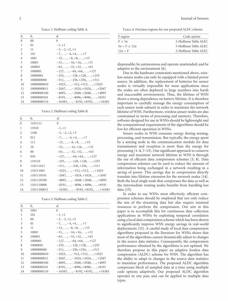
Table 1: Huffman coding Table A.

bi hi di0 00 01 01 −1, +12 11 −3,−2, +2, +33 101 −7, . . . ,−4, +4, . . . , +74 1001 −15, . . . ,−8, +8, . . . , +155 10001 −31, . . . ,−16, +16, . . . , +316 100001 −63, . . . ,−32, +32, . . . , +637 1000001 −127, . . . ,−64, +64, . . . , +1278 10000001 −255, . . . ,−128, +128, . . . , +2559 1000000000 −511, . . . ,−256, +256, . . . , +51110 10000000010 −1023, . . . ,−512, +512, . . . , +102311 10000000011 −2047, . . . ,−1024, +1024, . . . , +204712 10000000100 −4095, . . . ,−2048, +2048, . . . , +409513 10000000101 −8191, . . . ,−4096, +4096, . . . , +819114 10000000110 −16383, . . . ,−8192, +8192, . . . , +16383

Table 2: Huffman coding Table B.

bi hi di

0 1101111 0

1 11010 −1, +1

2 1100 −3,−2, +2, +3

3 011 −7, . . . ,−4, +4, . . . , +7

4 111 −15, . . . ,−8, +8, . . . , +15

5 10 −31, . . . ,−16, +16, . . . , +31

6 00 −63, . . . ,−32, +32, . . . , +63

7 010 −127, . . . ,−64, +64, . . . , +127

8 110110 −255, . . . ,−128, +128, . . . , +255

9 110111011 −511, . . . ,−256, +256, . . . , +511

10 110111001 −1023, . . . ,−512, +512, . . . , +1023

11 1101110101 −2047, . . . ,−1024, +1024, . . . , +2047

12 1101110100 −4095, . . . ,−2048, +2048, . . . , +4095

13 1101110000 −8191, . . . ,−4096, +4096, . . . , +8191

14 11011100011 −16383, . . . ,−8192, +8192, . . . , +16383

Table 3: Huffman coding Table C.

bi hi di0 1001 01 101 −1, +12 00 −3,−2, +2, +33 01 −7, . . . ,−4, +4, . . . , +74 11 −15, . . . ,−8, +8, . . . , +155 10001 −31, . . . ,−16, +16, . . . , +316 100001 −63, . . . ,−32, +32, . . . , +637 1000001 −127, . . . ,−64, +64, . . . , +1278 10000001 −255, . . . ,−128, +128, . . . , +2559 1000000000 −511, . . . ,−256, +256, . . . , +51110 10000000010 −1023, . . . ,−512, +512, . . . , +102311 10000000011 −2047, . . . ,−1024, +1024, . . . , +204712 10000000100 −4095, . . . ,−2048, +2048, . . . , +409513 10000000101 −8191, . . . ,−4096, +4096, . . . , +819114 10000000110 −16383, . . . ,−8192, +8192, . . . , +16383

Table 4: Decision regions for our proposed ALDC scheme.

F region Code option

F ≤ 3n 2-Huffman Table ALEC

3n < F ≤ 12n 3-Huffman Table ALEC

12n < F 2-Huffman Table ALEC

dispensable; be autonomous and operate unattended; and beadaptive to the environment [6].

Due to the hardware constraints mentioned above, wire-less sensor nodes can only be equipped with a limited powersource. In addition, the replacement of batteries for sensornodes is virtually impossible for most applications sincethe nodes are often deployed in large numbers into harshand inaccessible environments. Thus, the lifetime of WSNshows a strong dependence on battery lifetime. It is thereforeimportant to carefully manage the energy consumption ofeach sensor node subunit in order to maximize the networklifetime of WSN. Furthermore, wireless sensor nodes are alsoconstrained in terms of processing and memory. Therefore,software designed for use in WSNs should be lightweight andthe computational requirements of the algorithms should below for efficient operation in WSNs.

Sensor nodes in WSN consume energy during sensing,processing, and transmission. But typically, the energy spentby a sensing node in the communication module for datatransmission and reception is more than the energy forprocessing [1–4, 7–13]. One significant approach to conserveenergy and maximize network lifetime in WSN is throughthe use of efficient data compression schemes [5, 8]. Datacompression schemes can be used to reduce the amount ofinformation being exchanged in a network resulting in asaving of power. This savings due to compression directlytranslate into lifetime extension for the network nodes [14].Both the local single node that compresses the data as well asthe intermediate routing nodes benefits from handling lessdata [15].

In order to use WSNs most effectively, efficient com-pression schemes should be employed that not only reducethe size of the streaming data but also require minimalresources to perform the compression. Our aim in thispaper is to accomplish this for continuous data collectionapplications in WSNs by exploiting temporal correlationusing a local data compression scheme which has been shownto significantly improve WSN energy savings in real-worlddeployments [15]. A careful study of local data compressionalgorithms proposed in the literature for WSNs shows thatmost of the algorithms cannot dynamically adjust to changesin the source data statistics. Consequently, the compressionperformance obtained by the algorithms is not optimal. Wetherefore propose in this paper an adaptive lossless datacompression (ALDC) scheme for WSN. The algorithm hasthe ability to adapt to changes in the source data statisticsto maximize performance. The proposed ALDC algorithmcompresses block of sampled data at a time using multiplecode options adaptively. Our proposed ALDC algorithmoperates in one pass and can be applied to multiple datatypes.

Journal of Sensors 3

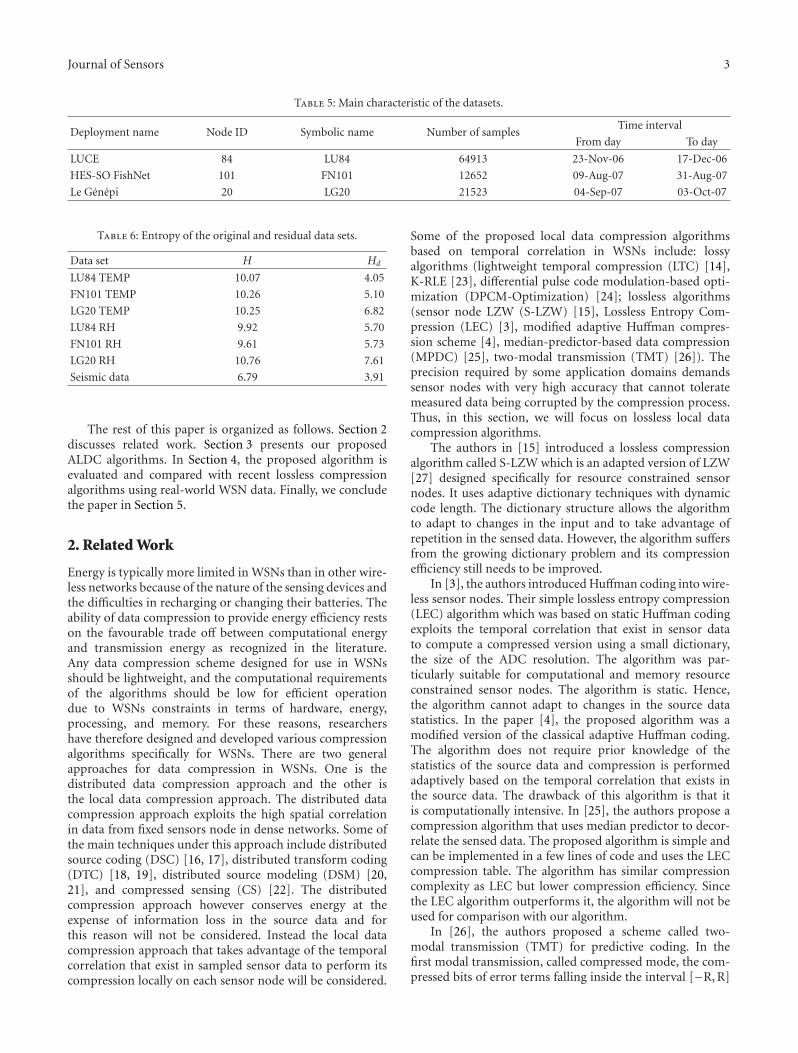
Table 5: Main characteristic of the datasets.

Deployment name Node ID Symbolic name Number of samplesTime interval

From day To day

LUCE 84 LU84 64913 23-Nov-06 17-Dec-06

HES-SO FishNet 101 FN101 12652 09-Aug-07 31-Aug-07

Le Genepi 20 LG20 21523 04-Sep-07 03-Oct-07

Table 6: Entropy of the original and residual data sets.

Data set H Hd

LU84 TEMP 10.07 4.05

FN101 TEMP 10.26 5.10

LG20 TEMP 10.25 6.82

LU84 RH 9.92 5.70

FN101 RH 9.61 5.73

LG20 RH 10.76 7.61

Seismic data 6.79 3.91

The rest of this paper is organized as follows. Section 2discusses related work. Section 3 presents our proposedALDC algorithms. In Section 4, the proposed algorithm isevaluated and compared with recent lossless compressionalgorithms using real-world WSN data. Finally, we concludethe paper in Section 5.

2. Related Work

Energy is typically more limited in WSNs than in other wire-less networks because of the nature of the sensing devices andthe difficulties in recharging or changing their batteries. Theability of data compression to provide energy efficiency restson the favourable trade off between computational energyand transmission energy as recognized in the literature.Any data compression scheme designed for use in WSNsshould be lightweight, and the computational requirementsof the algorithms should be low for efficient operationdue to WSNs constraints in terms of hardware, energy,processing, and memory. For these reasons, researchershave therefore designed and developed various compressionalgorithms specifically for WSNs. There are two generalapproaches for data compression in WSNs. One is thedistributed data compression approach and the other isthe local data compression approach. The distributed datacompression approach exploits the high spatial correlationin data from fixed sensors node in dense networks. Some ofthe main techniques under this approach include distributedsource coding (DSC) [16, 17], distributed transform coding(DTC) [18, 19], distributed source modeling (DSM) [20,21], and compressed sensing (CS) [22]. The distributedcompression approach however conserves energy at theexpense of information loss in the source data and forthis reason will not be considered. Instead the local datacompression approach that takes advantage of the temporalcorrelation that exist in sampled sensor data to perform itscompression locally on each sensor node will be considered.

Some of the proposed local data compression algorithmsbased on temporal correlation in WSNs include: lossyalgorithms (lightweight temporal compression (LTC) [14],K-RLE [23], differential pulse code modulation-based opti-mization (DPCM-Optimization) [24]; lossless algorithms(sensor node LZW (S-LZW) [15], Lossless Entropy Com-pression (LEC) [3], modified adaptive Huffman compres-sion scheme [4], median-predictor-based data compression(MPDC) [25], two-modal transmission (TMT) [26]). Theprecision required by some application domains demandssensor nodes with very high accuracy that cannot toleratemeasured data being corrupted by the compression process.Thus, in this section, we will focus on lossless local datacompression algorithms.

The authors in [15] introduced a lossless compressionalgorithm called S-LZW which is an adapted version of LZW[27] designed specifically for resource constrained sensornodes. It uses adaptive dictionary techniques with dynamiccode length. The dictionary structure allows the algorithmto adapt to changes in the input and to take advantage ofrepetition in the sensed data. However, the algorithm suffersfrom the growing dictionary problem and its compressionefficiency still needs to be improved.

In [3], the authors introduced Huffman coding into wire-less sensor nodes. Their simple lossless entropy compression(LEC) algorithm which was based on static Huffman codingexploits the temporal correlation that exist in sensor datato compute a compressed version using a small dictionary,the size of the ADC resolution. The algorithm was par-ticularly suitable for computational and memory resourceconstrained sensor nodes. The algorithm is static. Hence,the algorithm cannot adapt to changes in the source datastatistics. In the paper [4], the proposed algorithm was amodified version of the classical adaptive Huffman coding.The algorithm does not require prior knowledge of thestatistics of the source data and compression is performedadaptively based on the temporal correlation that exists inthe source data. The drawback of this algorithm is that itis computationally intensive. In [25], the authors propose acompression algorithm that uses median predictor to decor-relate the sensed data. The proposed algorithm is simple andcan be implemented in a few lines of code and uses the LECcompression table. The algorithm has similar compressioncomplexity as LEC but lower compression efficiency. Sincethe LEC algorithm outperforms it, the algorithm will not beused for comparison with our algorithm.

In [26], the authors proposed a scheme called two-modal transmission (TMT) for predictive coding. In thefirst modal transmission, called compressed mode, the com-pressed bits of error terms falling inside the interval [−R, R]


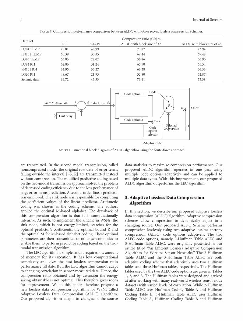
Table 7: Compression performance comparison between ALDC with other recent lossless compression schemes.

Data setCompression ratio (CR) %

LEC S-LZW ALDC with block size of 32 ALDC with block size of 48

LU84 TEMP 70.81 48.99 73.87 73.94

FN101 TEMP 65.39 30.35 67.44 67.48

LG20 TEMP 53.83 22.02 56.86 56.90

LU84 RH 62.86 31.24 65.50 65.54

FN101 RH 62.95 36.27 66.28 66.33

LG20 RH 48.67 21.93 52.80 52.87

Seismic data 69.72 43.33 73.41 73.38

Unit delay

+

−

Code option 1

Code option 2

Adaptive coder

Code

Code

Codeoptionselector

strm

IDSelectedcode option

xi = x1, x2, . . . , xn di = d1,d2, . . . ,dn

Figure 1: Functional block diagram of ALDC algorithm using the brute-force approach.

are transmitted. In the second modal transmission, callednoncompressed mode, the original raw data of error termsfalling outside the interval [−R, R] are transmitted insteadwithout compression. The modified predictive coding basedon the two-modal transmission approach solved the problemof decreased coding efficiency due to the low performance oflarge error terms prediction. A second-order linear predictorwas employed. The sink node was responsible for computingthe coefficient values of the linear predictor. Arithmeticcoding was chosen as the coding scheme. The authorsapplied the optimal M-based alphabet. The drawback ofthis compression algorithm is that it is computationallyintensive. As such, to implement the scheme in WSNs, thesink node, which is not energy-limited, searches for theoptimal predictor’s coefficients, the optimal bound R andthe optimal M for M-based alphabet coding. These optimalparameters are then transmitted to other sensor nodes toenable them to perform predictive coding based on the two-modal transmission algorithm.

The LEC algorithm is simple, and it requires low amountof memory for its execution. It has low computationalcomplexity and gives the best lossless compression ratioperformance till date. But, the LEC algorithm cannot adaptto changing correlation in sensor-measured data. Hence, thecompression ratio obtained and by extension the energysaving obtainable is not optimal. This therefore gives roomfor improvement. We in this paper, therefore propose anew lossless data compression algorithm for WSNs calledAdaptive Lossless Data Compression (ALDC) algorithm.Our proposed algorithm adapts to changes in the source

data statistics to maximize compression performance. Ourproposed ALDC algorithm operates in one pass usingmultiple code options adaptively and can be applied tomultiple data types. With this improvement, our proposedALDC algorithm outperforms the LEC algorithm.

3. Adaptive Lossless Data CompressionAlgorithm

In this section, we describe our proposed adaptive losslessdata compression (ALDC) algorithm. Adaptive compressionschemes allow compression to dynamically adjust to achanging source. Our proposed ALDC Scheme performscompression losslessly using two adaptive lossless entropycompression (ALEC) code options adaptively. The twoALEC code options, namely 2-Huffman Table ALEC and3-Huffman Table ALEC, were originally presented in ourarticle titled “An Efficient Lossless Adaptive CompressionAlgorithm for Wireless Sensor Networks.” The 2-HuffmanTable ALEC and the 3-Huffman Table ALEC are bothadaptive coding scheme that adaptively uses two Huffmantables and three Huffman tables, respectively. The Huffmantables used by the two ALEC code options are given in Tables1, 2, and 3. The Huffman tables were designed and arrivedat after working with many real-world wireless sensor nodedatasets with varied levels of correlation. While 2-HuffmanTable ALEC uses Huffman Coding Table A and HuffmanCoding Table B, 3-Huffman Table ALEC uses HuffmanCoding Table A, Huffman Coding Table B and Huffman


96 384 10002

3C

ode

opti

on p

aram

eter

Sum value of block of 32 residual samples absolute values

First boundary Second boundary

(a)

2

3

Cod

e op

tion

par

amet

er

10 96 384 1000



(b)

10 96 3842

3

Cod

e op

tion

par

amet

er


First boundary Secondboundary

(c)

2

3

Cod

e op

tion

par

amet

er

10 96 384 1000



(d)

96 3842

3

Cod

e op

tion

par

amet

er



1000

(e)

2

3

Cod

e op

tion

par

amet

er

10 96 384 1000 10000



(f)

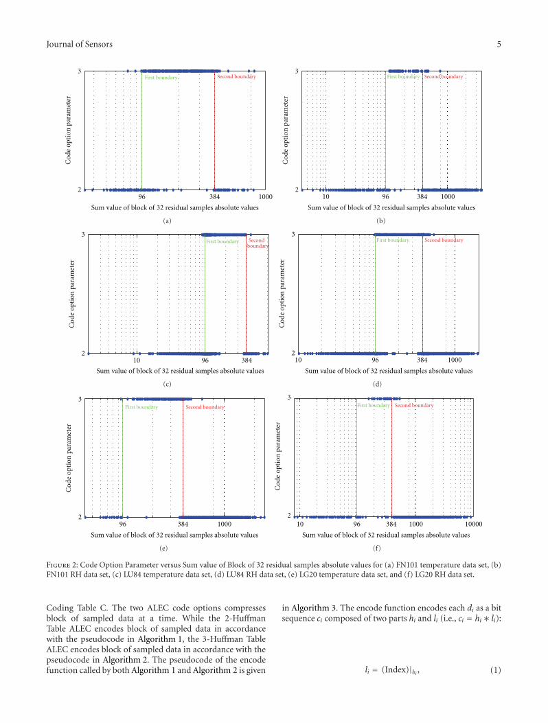
Figure 2: Code Option Parameter versus Sum value of Block of 32 residual samples absolute values for (a) FN101 temperature data set, (b)FN101 RH data set, (c) LU84 temperature data set, (d) LU84 RH data set, (e) LG20 temperature data set, and (f) LG20 RH data set.

Coding Table C. The two ALEC code options compressesblock of sampled data at a time. While the 2-HuffmanTable ALEC encodes block of sampled data in accordancewith the pseudocode in Algorithm 1, the 3-Huffman TableALEC encodes block of sampled data in accordance with thepseudocode in Algorithm 2. The pseudocode of the encodefunction called by both Algorithm 1 and Algorithm 2 is given

in Algorithm 3. The encode function encodes each di as a bitsequence ci composed of two parts hi and li (i.e., ci = hi ∗ li):

li = (Index)|bi , (1)


100 144 576 10002

3C

ode

opti

on p

aram

eter



(a)

2

3

Cod

e op

tion

par

amet

er

10 100 144 576 1000



(b)

2

3

Cod

e op

tion

par

amet

er

100 144 576 1000


First boundary Secondboundary

(c)

2

3

Cod

e op

tion

par

amet

er

100 144 576 1000



(d)

2

3

Cod

e op

tion

par

amet

er

100 144 576 1000



(e)

2

3

Cod

e op

tion

par

amet

er

100 144 576 1000 10000



(f)

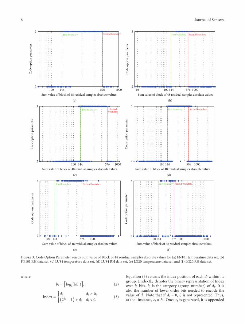
Figure 3: Code Option Parameter versus Sum value of Block of 48 residual samples absolute values for (a) FN101 temperature data set, (b)FN101 RH data set, (c) LU84 temperature data set, (d) LU84 RH data set, (e) LG20 temperature data set, and (f) LG20 RH data set.

where

bi =⌈

log2(|di|)⌉

, (2)

Index =⎧⎨⎩di di ≥ 0,(

2bi − 1)

+ di di < 0.(3)

Equation (3) returns the index position of each di within itsgroup. (Index)|bi denotes the binary representation of Indexover bi bits. bi is the category (group number) of di. It isalso the number of lower order bits needed to encode thevalue of di. Note that if di = 0, li is not represented. Thus,at that instance, ci = hi. Once ci is generated, it is appended


Unit delay

+

−

Code option 1

Code option 2

Adaptive coder

Code

Code

Codeoptionselector

strm

IDSelectedcode option

xi = x1, x2, . . . , xn di = d1,d2, . . . ,dn

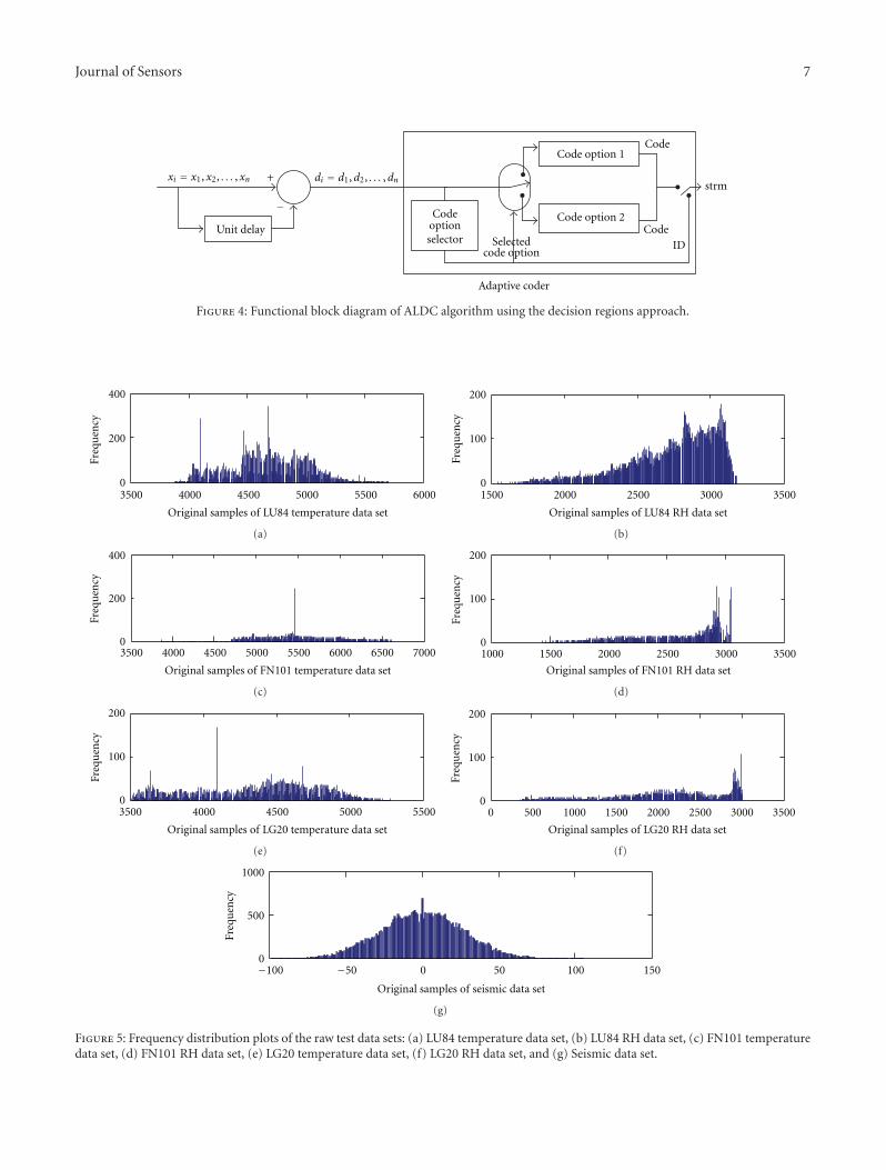
Figure 4: Functional block diagram of ALDC algorithm using the decision regions approach.

3500 4000 4500 5000 5500 6000

Original samples of LU84 temperature data set

0

200

400

Freq

uen

cy

(a)

1500 2000 2500 3000 35000

100

200

Freq

uen

cy

Original samples of LU84 RH data set

(b)

0

200

400

Freq

uen

cy

3500 4000 4500 5000 5500 6000 6500 7000

Original samples of FN101 temperature data set

(c)

1000 1500 2000 2500 3000 3500

Original samples of FN101 RH data set

0

100

200

Freq

uen

cy

(d)

0

100

200

Freq

uen

cy

3500 4000 4500 5000 5500

Original samples of LG20 temperature data set

(e)

0

100

200

Freq

uen

cy

0 500 1000 1500 2000 2500 3000 3500

Original samples of LG20 RH data set

(f)

−100 −50 0 50 100 1500

500

1000

Freq

uen

cy

Original samples of seismic data set

(g)

Figure 5: Frequency distribution plots of the raw test data sets: (a) LU84 temperature data set, (b) LU84 RH data set, (c) FN101 temperaturedata set, (d) FN101 RH data set, (e) LG20 temperature data set, (f) LG20 RH data set, and (g) Seismic data set.


0 100 2000

1

2

Freq

uen

cy

Residues of LU84 temperature data set

−200 −100

×104

(a)

0 100 200 3000

5000

10000

Freq

uen

cy

Residues of LU84 RH set

−200−300 −100

(b)

0

1000

2000

Freq

uen

cy

Residues of FN101 temperature data set

0 100 200−200 −100

(c)

0

2000

4000

Freq

uen

cy

Residues of FN101 RH data set

0 100 200 300−200−300 −100

(d)

0

500

1000

Freq

uen

cy

Residues of LG20 temperature data set

0 100 200−200 −100

(e)

0

1000

2000Fr

equ

ency

Residues of LG20 RH data set

0 100 200 300−200−300 −100

(f)

0

2000

4000

Freq

uen

cy

−200 −150 −100 −50 0 50 100 150 200

Residues of seismic data set

(g)

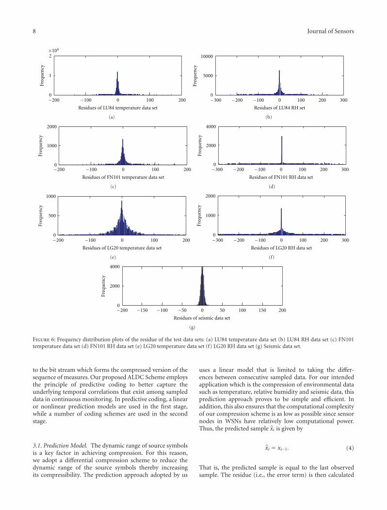
Figure 6: Frequency distribution plots of the residue of the test data sets: (a) LU84 temperature data set (b) LU84 RH data set (c) FN101temperature data set (d) FN101 RH data set (e) LG20 temperature data set (f) LG20 RH data set (g) Seismic data set.

to the bit stream which forms the compressed version of thesequence of measures. Our proposed ALDC Scheme employsthe principle of predictive coding to better capture theunderlying temporal correlations that exist among sampleddata in continuous monitoring. In predictive coding, a linearor nonlinear prediction models are used in the first stage,while a number of coding schemes are used in the secondstage.

3.1. Prediction Model. The dynamic range of source symbolsis a key factor in achieving compression. For this reason,we adopt a differential compression scheme to reduce thedynamic range of the source symbols thereby increasingits compressibility. The prediction approach adopted by us

uses a linear model that is limited to taking the differ-ences between consecutive sampled data. For our intendedapplication which is the compression of environmental datasuch as temperature, relative humidity and seismic data, thisprediction approach proves to be simple and efficient. Inaddition, this also ensures that the computational complexityof our compression scheme is as low as possible since sensornodes in WSNs have relatively low computational power.Thus, the predicted sample xi is given by

xi = xi−1. (4)

That is, the predicted sample is equal to the last observedsample. The residue (i.e., the error term) is then calculated


62

64

66

68

70

72

74

76

CR

(%

)

0 50 100 150 200 250 300 350

Block size

CR versus block size (LU84 temperature data set)

Figure 7: CR versus block size achieved by the ALDC algorithm forthe LU84 temperature data set using the brute-force approach.

0 50 100 150 200 250 300 35058

59

60

61

62

63

64

65

66

67

68

CR

(%

)

Block size

CR versus block size (FN101 temperature data set)

Figure 8: CR versus block size achieved by the ALDC algorithm forthe FN101 temperature data set using the brute-force approach.

by subtracting the predicted sample from the current sample.Hence, the residue di is the difference

di = xi − xi−1. (5)

In order to compute the first residue d1 we assume that

x0 = 2R−1, (6)

where R is the default measurement resolution of theincoming data set (i.e., R is the dynamic range of the sourcesymbols under consideration). Note, each xi is a positive-integer value in the range [0, 2R − 1] and it is representedin binary on R bits. We choose x0 to be equal to thecentral positive-integer value among the 2R possible positive-integer values. In our intended application using the testdatasets, the default measurement resolution for the relative

0 50 100 150 200 250 300 35048

49

50

51

52

53

54

55

56

57

CR

(%

)

Block size

CR versus block size (LG20 temperature data set)

Figure 9: CR versus block size achieved by the ALDC algorithm forthe LG20 temperature data set using the brute-force approach.

0 50 100 150 200 250 300 35056

57

58

59

60

61

62

63

64

65

66

CR

(%

)

Block size

CR versus block size (LU84 relative humidity data set)

Figure 10: CR versus block size achieved by the ALDC algorithmfor the LU84 relative humidity data set using the brute-forceapproach.

humidity and temperature datasets is 12 bits and 14 bits,respectively. Therefore, for each application, x0 is known byboth the encoder and decoder. Consequently, the algorithmis adaptable to different data sources since x0 is related to theincoming data. The computed residue di is then used as inputto the entropy encoder. That is, di is used to losslessly encodexi using the coding schemes described in Section 3.2.

3.2. Entropy Coding. In order to achieve maximal compres-sion ratio and by extension maximal energy saving, wepropose to implement ALDC algorithm that compressesblocks of sampled data at a time using two ALEC codeoptions adaptively. Our proposed ALDC algorithm operatesin one pass and can be applied to different data types. Our


0 50 100 150 200 250 300 35056

58

60

62

64

66

68

CR

(%

)

Block size

CR versus block size (FN101 relative humidity data set)

Figure 11: CR versus block size achieved by the ALDC algorithmfor the FN101 relative humidity data set using the brute-forceapproach.

0 50 100 150 200 250 300 35043

44

45

46

47

48

49

50

51

52

53

CR

(%

)

Block size

CR versus block size (LG20 relative humidity data set)

Figure 12: CR versus block size achieved by the ALDC algorithmfor the LG20 relative humidity data set using the brute-forceapproach.

entropy coding problem is how to efficiently encode blockof n integer-valued samples at a time using two ALEC codeoptions adaptively. Two different approaches to solve thisentropy coding problem will be discussed in this section. Theapproaches are, namely, the brute-force approach and thedecision regions approach.

3.2.1. The Brute-Force Approach. Figure 1 shows the func-tional block diagram of the implementation of the ALDCalgorithm using the brute-force approach. Code option 1and code option 2 represents 2-Huffman Table ALEC and3-Huffman Table ALEC, respectively. From Figure 1, theblock of n-samples xi is preprocessed by the simple unit-delay predictor to obtain block of n-residues di. di is then

0 50 100 150 200 250 300 35062

64

66

68

70

72

74

CR

(%

)

Block size

CR versus block size (seismic data set)

Figure 13: CR versus block size achieved by the ALDC algorithmfor the Seismic data set using the brute-force approach.

0 50 100 150 200 250 300 35062

64

66

68

70

72

74

76C

R (

%)

Block size


Figure 14: CR versus block size achieved by the ALDC algorithmfor the LU84 temperature data set using the decision regionsapproach.

encoded (compressed) by the adaptive coder using both codeoptions. The sizes of the encoded bitstreams generated byusing the two code options are then compared. The codeoption that yields the smallest encoded bitstream size (i.e.,highest compression) is then selected. The encoded bitstreamgenerated by this code option is then appended to the codeoption identifier (ID) and thereafter sent to the sink. Thedecoder uses the ID to identify the code option used inencoding di. Repeat the procedure until the end of the sourcedata is reached. The pseudocode of the compress functionusing the brute-force approach is given in Algorithm 4. Thebrute-force approach guarantees that optimal compressionratio is attained for each data set since it is always the bestcode option that is selected for each block of n samples.However, the brute-force approach requires more memory


0 50 100 150 200 250 300 35058

59

60

61

62

63

64

65

66

67

68

CR

(%

)

Block size


Figure 15: CR versus block size achieved by the ALDC algorithmfor the FN101 temperature data set using the decision regionsapproach.

0 50 100 150 200 250 300 35048

49

50

51

52

53

54

55

56

57

CR

(%

)

Block size


Figure 16: CR versus block size achieved by the ALDC algorithmfor the LG20 temperature data set using the decision regionsapproach.

(for buffering the encoded bitstreams of both code optionsfor comparison) and it is also computational intensive (sinceencoding is done by both code options for each block of n-samples di).

3.2.2. The Decision Regions Approach. As stated inSection 3.2.1, the brute-force approach requires morememory (for buffering the encoded bitstreams of bothcode options for comparison) and it is also computationalintensive (since encoding is done by both code options foreach block of n-samples di). However, the sensor node hasstringent constraint in terms of memory, computationalpower and energy. We therefore turn our attention to theissue of selecting a code option that efficiently encode block

0 50 100 150 200 250 300 35056

57

58

59

60

61

62

63

64

65

66

CR

(%

)

Block size


Figure 17: CR versus block size achieved by the ALDC algorithmfor the LU84 relative humidity data set using the decision regionsapproach.

0 50 100 150 200 250 300 35054

56

58

60

62

64

66

68

CR

(%

)

Block size


Figure 18: CR versus block size achieved by the ALDC algorithmfor the FN101 relative humidity data set using the decision regionsapproach.

of n-samples di without using the brute-force approachsince it has been shown that the approach is unnecessarilycomplex. In [28], the authors introduced a high performanceadaptive coding module using the brute-force approachin the selection of a code option. Because the brute-forceapproach is computationally exhaustive and/or hardwaredemanding, the authors later proposed a simpler alternativeto the brute-force approach that uses a table of decisionregions that is solely based on the length of the fundamentalsequence of n-standard source samples (nonnegativeintegers). The length of the fundamental sequence ofn-standard source samples is essentially the sum of then-standard source samples in a block plus n (the blocksize). The calculated sum is then used alongside the table of


0 50 100 150 200 250 300 35043

44

45

46

47

48

49

50

51

52

53

CR

(%

)

Block size


Figure 19: CR versus block size achieved by the ALDC algorithmfor the LG20 relative humidity data set using the decision regionsapproach.

0 50 100 150 200 250 300 35062

64

66

68

70

72

74

CR

(%

)

Block size


Figure 20: CR versus block size achieved by the ALDC algorithmfor the Seismic data set using the decision regions approach.

decision regions to select the best code option for encoding.Thus, under this new approach, only one code option wasused per block of n-standard source samples. This led to alot of savings in times of both computational requirementsand hardware. Motivated by the simplicity of this decisionregions approach, we set out to find out if for our proposedALDC we can use similar decision regions approach definedsolely by certain sum expression for best code optionselection using empirical method.

To this end, using the brute-force approach discussed inSection 3.2.1 alongside its pseudocode in Algorithm 4, wegenerate the pattern of code options usage while compressingeach data set by repeating the following procedures for eachblock of n-residues di until the end of the data set is reached:

0 50 100 150 200 250 300 35062

64

66

68

70

72

74

76

CR

(%

)

Block size


The brute-force approachThe decision regions approach

Figure 21: Performance comparison between the brute-forceapproach and the decision regions approach of ALDC for the Lu84temperature data set.

0 50 100 150 200 250 300 35058

59

60

61

62

63

64

65

66

67

68

CR

(%

)

Block size



Figure 22: Performance comparison between the brute-forceapproach and the decision regions approach of ALDC for the FN101temperature data set.

(a) Compute the sum of the absolute value of eachresidual sample in a block of n-residues di. Store thecomputed sum in the SUM array.

(b) Encode (compress) the block of n-residues di usingboth code options (namely, 2-Huffman Table ALECand 3-Huffman Table ALEC).

(c) Select the best code option that yields the smallestencoded bitstream size for each block of n-residuesdi. If 2-Huffman Table ALEC is the best code optionselected, then the code option identifier (ID) of 2 isgenerated and stored in the ID array, otherwise the


0 50 100 150 200 250 300 35048

49

50

51

52

53

54

55

56

57

CR

(%

)

Block size



Figure 23: Performance comparison between the brute-forceapproach and the decision regions approach of ALDC for the LG20temperature data set.

0 50 100 150 200 250 300 35056

57

58

59

60

61

62

63

64

65

66

CR

(%

)

Block size


The brute-force approach

The decision regions approach

Figure 24: Performance comparison between the brute-forceapproach and the decision regions approach of ALDC for the Lu84relative humidity data set.

code option identifier (ID) of 3 is generated insteadand stored in ID array.

Procedures (a) to (c) are repeated for block sizes of 32and 48 for different data sets. Thereafter, we plotted theID arrays against the corresponding SUM arrays using datamarkers only for the different test data sets. These plots aregiven in Figures 2 and 3 for block size of 32 and 48 samples,respectively. Note that, some of the data points in the plotsare plotted several times. As seen from the plots (Figures

0 50 100 150 200 250 300 35054

56

58

60

62

64

66

68

CR

(%

)

Block size


The brute-force approach

The decision regions approach

Figure 25: Performance comparison between the brute-forceapproach and the decision regions approach of ALDC for the FN101relative humidity data set.

0 50 100 150 200 250 300 35043

44

45

46

47

48

49

50

51

52

53

CR

(%

)

Block size



Figure 26: Performance comparison between the brute-forceapproach and the decision regions approach of ALDC for the LG20relative humidity data set.

2 and 3), the compression performance of the two codeoptions overlaps at two regions. For the block size of 32, thetwo regions are the sum values in the range [80, 112] and[368, 400]. Similarly, for block size of 48, the two regionswithin which the performance of the two code optionsoverlaps are the sum values in the range [120, 168] and[552, 600]. Depending on the block size (32 or 48), any sumvalue in these two regions can be used as decision regionsboundary sum value resulting in approximately the same


0 50 100 150 200 250 300 35062

64

66

68

70

72

74

CR

(%

)

Block size



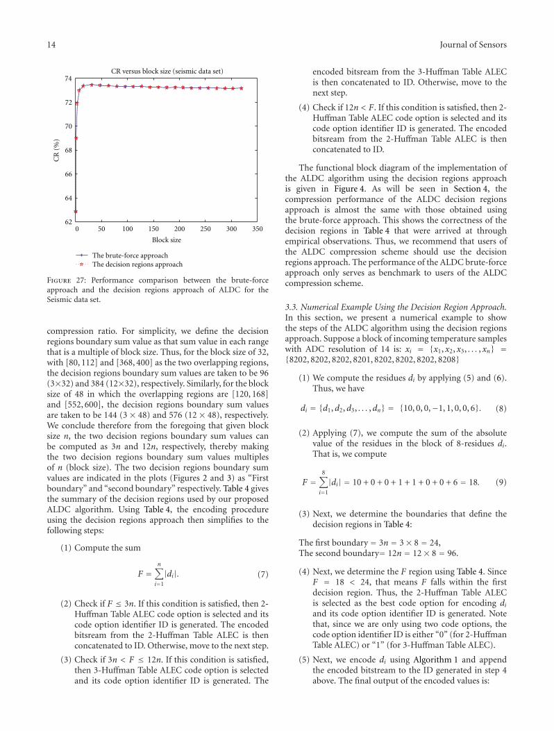
Figure 27: Performance comparison between the brute-forceapproach and the decision regions approach of ALDC for theSeismic data set.

compression ratio. For simplicity, we define the decisionregions boundary sum value as that sum value in each rangethat is a multiple of block size. Thus, for the block size of 32,with [80, 112] and [368, 400] as the two overlapping regions,the decision regions boundary sum values are taken to be 96(3×32) and 384 (12×32), respectively. Similarly, for the blocksize of 48 in which the overlapping regions are [120, 168]and [552, 600], the decision regions boundary sum valuesare taken to be 144 (3 × 48) and 576 (12 × 48), respectively.We conclude therefore from the foregoing that given blocksize n, the two decision regions boundary sum values canbe computed as 3n and 12n, respectively, thereby makingthe two decision regions boundary sum values multiplesof n (block size). The two decision regions boundary sumvalues are indicated in the plots (Figures 2 and 3) as “Firstboundary” and “second boundary” respectively. Table 4 givesthe summary of the decision regions used by our proposedALDC algorithm. Using Table 4, the encoding procedureusing the decision regions approach then simplifies to thefollowing steps:

(1) Compute the sum

F =n∑

i=1

|di|. (7)

(2) Check if F ≤ 3n. If this condition is satisfied, then 2-Huffman Table ALEC code option is selected and itscode option identifier ID is generated. The encodedbitsream from the 2-Huffman Table ALEC is thenconcatenated to ID. Otherwise, move to the next step.

(3) Check if 3n < F ≤ 12n. If this condition is satisfied,then 3-Huffman Table ALEC code option is selectedand its code option identifier ID is generated. The

encoded bitsream from the 3-Huffman Table ALECis then concatenated to ID. Otherwise, move to thenext step.

(4) Check if 12n < F. If this condition is satisfied, then 2-Huffman Table ALEC code option is selected and itscode option identifier ID is generated. The encodedbitsream from the 2-Huffman Table ALEC is thenconcatenated to ID.

The functional block diagram of the implementation ofthe ALDC algorithm using the decision regions approachis given in Figure 4. As will be seen in Section 4, thecompression performance of the ALDC decision regionsapproach is almost the same with those obtained usingthe brute-force approach. This shows the correctness of thedecision regions in Table 4 that were arrived at throughempirical observations. Thus, we recommend that users ofthe ALDC compression scheme should use the decisionregions approach. The performance of the ALDC brute-forceapproach only serves as benchmark to users of the ALDCcompression scheme.

3.3. Numerical Example Using the Decision Region Approach.In this section, we present a numerical example to showthe steps of the ALDC algorithm using the decision regionsapproach. Suppose a block of incoming temperature sampleswith ADC resolution of 14 is: xi = {x1, x2, x3, . . . , xn} ={8202, 8202, 8202, 8201, 8202, 8202, 8202, 8208}

(1) We compute the residues di by applying (5) and (6).Thus, we have

di = {d1,d2,d3, . . . ,dn} = {10, 0, 0,−1, 1, 0, 0, 6}. (8)

(2) Applying (7), we compute the sum of the absolutevalue of the residues in the block of 8-residues di.That is, we compute

F =8∑

i=1

|di| = 10 + 0 + 0 + 1 + 1 + 0 + 0 + 6 = 18. (9)

(3) Next, we determine the boundaries that define thedecision regions in Table 4:

The first boundary = 3n = 3× 8 = 24,The second boundary= 12n = 12× 8 = 96.

(4) Next, we determine the F region using Table 4. SinceF = 18 < 24, that means F falls within the firstdecision region. Thus, the 2-Huffman Table ALECis selected as the best code option for encoding diand its code option identifier ID is generated. Notethat, since we are only using two code options, thecode option identifier ID is either “0” (for 2-HuffmanTable ALEC) or “1” (for 3-Huffman Table ALEC).

(5) Next, we encode di using Algorithm 1 and appendthe encoded bitstream to the ID generated in step 4above. The final output of the encoded values is:


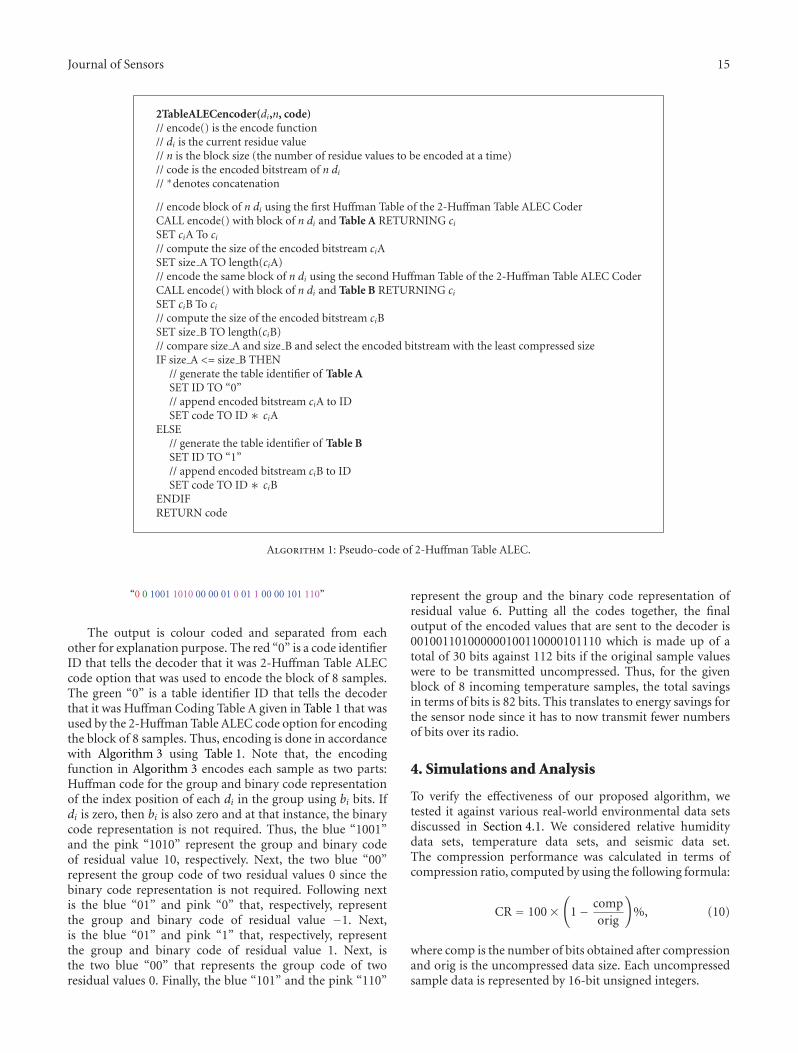
2TableALECencoder(di,n, code)// encode() is the encode function// di is the current residue value// n is the block size (the number of residue values to be encoded at a time)// code is the encoded bitstream of n di// ∗denotes concatenation

// encode block of n di using the first Huffman Table of the 2-Huffman Table ALEC CoderCALL encode() with block of n di and Table A RETURNING ciSET ciA To ci// compute the size of the encoded bitstream ciASET size A TO length(ciA)// encode the same block of n di using the second Huffman Table of the 2-Huffman Table ALEC CoderCALL encode() with block of n di and Table B RETURNING ciSET ciB To ci// compute the size of the encoded bitstream ciBSET size B TO length(ciB)// compare size A and size B and select the encoded bitstream with the least compressed sizeIF size A <= size B THEN

// generate the table identifier of Table ASET ID TO “0”// append encoded bitstream ciA to IDSET code TO ID ∗ ciA

ELSE// generate the table identifier of Table BSET ID TO “1”// append encoded bitstream ciB to IDSET code TO ID ∗ ciB

ENDIFRETURN code

Algorithm 1: Pseudo-code of 2-Huffman Table ALEC.

“0 0 1001 1010 00 00 01 0 01 1 00 00 101 110”

The output is colour coded and separated from eachother for explanation purpose. The red “0” is a code identifierID that tells the decoder that it was 2-Huffman Table ALECcode option that was used to encode the block of 8 samples.The green “0” is a table identifier ID that tells the decoderthat it was Huffman Coding Table A given in Table 1 that wasused by the 2-Huffman Table ALEC code option for encodingthe block of 8 samples. Thus, encoding is done in accordancewith Algorithm 3 using Table 1. Note that, the encodingfunction in Algorithm 3 encodes each sample as two parts:Huffman code for the group and binary code representationof the index position of each di in the group using bi bits. Ifdi is zero, then bi is also zero and at that instance, the binarycode representation is not required. Thus, the blue “1001”and the pink “1010” represent the group and binary codeof residual value 10, respectively. Next, the two blue “00”represent the group code of two residual values 0 since thebinary code representation is not required. Following nextis the blue “01” and pink “0” that, respectively, representthe group and binary code of residual value −1. Next,is the blue “01” and pink “1” that, respectively, representthe group and binary code of residual value 1. Next, isthe two blue “00” that represents the group code of tworesidual values 0. Finally, the blue “101” and the pink “110”

represent the group and the binary code representation ofresidual value 6. Putting all the codes together, the finaloutput of the encoded values that are sent to the decoder is001001101000000100110000101110 which is made up of atotal of 30 bits against 112 bits if the original sample valueswere to be transmitted uncompressed. Thus, for the givenblock of 8 incoming temperature samples, the total savingsin terms of bits is 82 bits. This translates to energy savings forthe sensor node since it has to now transmit fewer numbersof bits over its radio.

4. Simulations and Analysis

To verify the effectiveness of our proposed algorithm, wetested it against various real-world environmental data setsdiscussed in Section 4.1. We considered relative humiditydata sets, temperature data sets, and seismic data set.The compression performance was calculated in terms ofcompression ratio, computed by using the following formula:

CR = 100×(

1− comporig

)%, (10)

where comp is the number of bits obtained after compressionand orig is the uncompressed data size. Each uncompressedsample data is represented by 16-bit unsigned integers.


3TableALECencoder(di,n, code)// encode() is the encode function// di is the current residue value// n is the block size (the number of residue values to be encoded at a time)// code is the encoded bitstream of n di// ∗denotes concatenation

// encode block of n di using the first Huffman Table of the 3-Huffman Table ALEC CoderCALL encode() with block of n di and Table A RETURNING ciSET ciA To ci// compute the size of the encoded bitstream ciASET size A TO length(ciA)// encode the same block of n di using the second Huffman Table of the 3-Huffman Table ALEC CoderCALL encode() with block of n di and Table B RETURNING ciSET ciB To ci// compute the size of the encoded bitstream ciBSET size B TO length(ciB)// encode the same block of n di using the third Huffman Table of the 3-Huffman Table ALEC CoderCALL encode() with block of n di and Table C RETURNING ciSET ciC To ci// compute the size of the encoded bitstream ciCSET size C TO length(ciC)// compare size A, size B and size C and select the encoded bitstream with the least compressed sizeIF size A <= min(size B, size C) THEN

// generate the table identifier of Table ASET ID TO “10”// append encoded bitstream ciA to IDSET code TO ID ∗ ciA

ELSEIF size B <= min(size A, size C) THEN// generate the table identifier of Table BSET ID TO “11”// append encoded bitstream ciB to IDSET code TO ID ∗ ciB

ELSEIF size C <= min(size A, size B) THEN// generate the table identifier of Table CSET ID TO “0”// append encoded bitstream ciC to IDSET code TO ID ∗ ciC

ENDIFRETURN code

Algorithm 2: Pseudo-code of 3-Huffman Table ALEC.

4.1. Data Sets. Real-world environmental monitoring WSNdatasets from SensorScope [29] were used in our simulations.We used relative humidity and temperature measurementsfrom three SensorScope deployments: Le Genepi Deploy-ment, HES-SO FishNet Deployment and LUCE Deployment.Publicly accessible data sets were used to make the compar-ison as fair as possible. These deployments use a TinyNodenode [30] which comprises of a TI MSP430 microcontroller,a Xemics XE120,5 radio and a Sensirion SHT75 sensormodule [31]. Both the relative humidity and temperaturesensors are connected to a 14-bit analog-to-digital converter(ADC). The default measurement resolution for raw relativehumidity (raw h) and raw temperature (raw t) is 12 bits and14 bits respectively. Each ADC output raw h and raw t areconverted into measure h and t in percentage and degreeCelsius respectively as described in [31]. The data sets thatare published on SensorScope deployments correspond to

physical measures h and t. But the compression algorithmswork on raw h and raw t. Therefore, before applying thecompression algorithm, the physical measures h and t areconverted to raw h and raw t by using the inverted versionsof the conversion functions in [31]. Table 5 summarizes themain characteristics of the datasets. See [3] for further detailsregarding the characteristics of these data sets. In addition,we also used a seismic data set collected by the OhioSeisDigital Seismographic Station located in Bowling Green,Ohio, for the time interval of 2:00 PM to 3:00 PM on 21September 1999 (UT) [32]. We compute the informationentropy H = −∑N

i=1 p(xi)· log2p(xi) of the original data sets,where N is the number of possible values of xi (the output ofthe ADC) and p(xi) is the probability mass function of xi.In addition, the information entropy Hd = −∑N

i=1 p(di) ·log2p(di) of the residual signal was also computed. These areall recorded in Table 6.


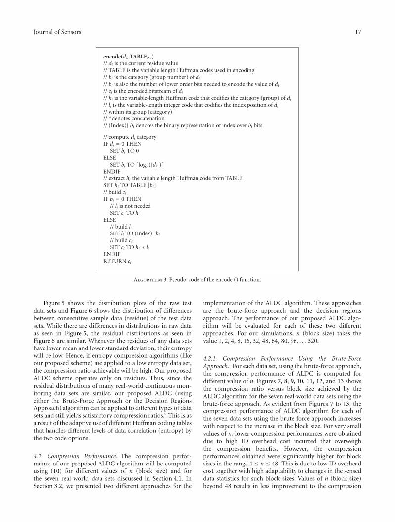
encode(di, TABLE,ci)// di is the current residue value// TABLE is the variable length Huffman codes used in encoding// bi is the category (group number) of di// bi is also the number of lower order bits needed to encode the value of di// ci is the encoded bitstream of di// hi is the variable-length Huffman code that codifies the category (group) of di// li is the variable-length integer code that codifies the index position of di// within its group (category)// ∗denotes concatenation// (Index)| bi denotes the binary representation of index over bi bits

// compute di categoryIF di = 0 THEN

SET bi TO 0ELSE

SET bi TO �log2 (|di|)�ENDIF// extract hi the variable length Huffman code from TABLESET hi TO TABLE [bi]// build ciIF bi = 0 THEN

// li is not neededSET ci TO hi

ELSE// build liSET li TO (Index)| bi// build ciSET ci TO hi ∗ li

ENDIFRETURN ci

Algorithm 3: Pseudo-code of the encode () function.

Figure 5 shows the distribution plots of the raw testdata sets and Figure 6 shows the distribution of differencesbetween consecutive sample data (residue) of the test datasets. While there are differences in distributions in raw dataas seen in Figure 5, the residual distributions as seen inFigure 6 are similar. Whenever the residues of any data setshave lower mean and lower standard deviation, their entropywill be low. Hence, if entropy compression algorithms (likeour proposed scheme) are applied to a low entropy data set,the compression ratio achievable will be high. Our proposedALDC scheme operates only on residues. Thus, since theresidual distributions of many real-world continuous mon-itoring data sets are similar, our proposed ALDC (usingeither the Brute-Force Approach or the Decision RegionsApproach) algorithm can be applied to different types of datasets and still yields satisfactory compression ratios.” This is asa result of the adaptive use of different Huffman coding tablesthat handles different levels of data correlation (entropy) bythe two code options.

4.2. Compression Performance. The compression perfor-mance of our proposed ALDC algorithm will be computedusing (10) for different values of n (block size) and forthe seven real-world data sets discussed in Section 4.1. InSection 3.2, we presented two different approaches for the

implementation of the ALDC algorithm. These approachesare the brute-force approach and the decision regionsapproach. The performance of our proposed ALDC algo-rithm will be evaluated for each of these two differentapproaches. For our simulations, n (block size) takes thevalue 1, 2, 4, 8, 16, 32, 48, 64, 80, 96, . . . 320.

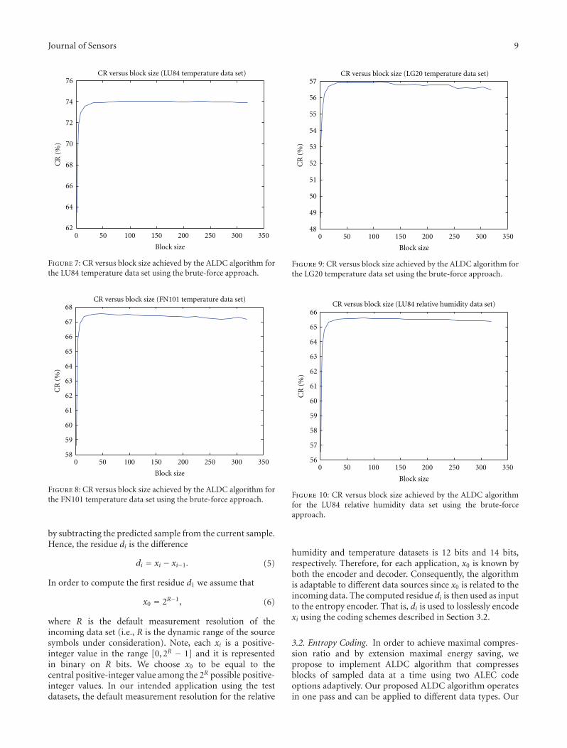
4.2.1. Compression Performance Using the Brute-ForceApproach. For each data set, using the brute-force approach,the compression performance of ALDC is computed fordifferent value of n. Figures 7, 8, 9, 10, 11, 12, and 13 showsthe compression ratio versus block size achieved by theALDC algorithm for the seven real-world data sets using thebrute-force approach. As evident from Figures 7 to 13, thecompression performance of ALDC algorithm for each ofthe seven data sets using the brute-force approach increaseswith respect to the increase in the block size. For very smallvalues of n, lower compression performances were obtaineddue to high ID overhead cost incurred that overweighthe compression benefits. However, the compressionperformances obtained were significantly higher for blocksizes in the range 4 ≤ n ≤ 48. This is due to low ID overheadcost together with high adaptability to changes in the senseddata statistics for such block sizes. Values of n (block size)beyond 48 results in less improvement to the compression


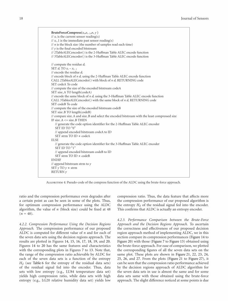
BruteForceCompress(xi,xi−1,n, y )// xi is the current sensor reading(s)// xi 1 is the immediate past sensor reading(s)// n is the block size (the number of samples read each time)// y is the final encoded bitstream// 2TableALECencoder() is the 2-Huffman Table ALEC encode function// 3TableALECencoder() is the 3-Huffman Table ALEC encode function

// compute the residue diSET di TO xi – xi−1

// encode the residue di// encode block of n di using the 2-Huffman Table ALEC encode functionCALL 2TablesALECencoder() with block of n di RETURNING codeSET codeA To code// compute the size of the encoded bitstream codeASET size A TO length(codeA)// encode the same block of n di using the 3-Huffman Table ALEC encode functionCALL 3TablesALECencoder() with the same block of n di RETURNING codeSET codeB To code// compute the size of the encoded bitstream codeBSET size B TO length(codeB)// compare size A and size B and select the encoded bitstream with the least compressed sizeIF size A <= size B THEN

// generate the code option identifier for the 2-Huffman Table ALEC encoderSET ID TO “0”// append encoded bitstream codeA to IDSET strm TO ID ∗ codeA

ELSE// generate the code option identifier for the 3-Huffman Table ALEC encoderSET ID TO “1”// append encoded bitstream codeB to IDSET strm TO ID ∗ codeB

ENDIF// append bitstream strm to ySET y TO y ∗ strmRETURN y

Algorithm 4: Pseudo-code of the compress function of the ALDC using the brute-force approach.

ratio and the compression performance even degrades aftera certain point as can be seen in some of the plots. Thus,for optimum compression performance using the ALDCalgorithm, the value of n (block size) could be fixed at 48(n = 48).

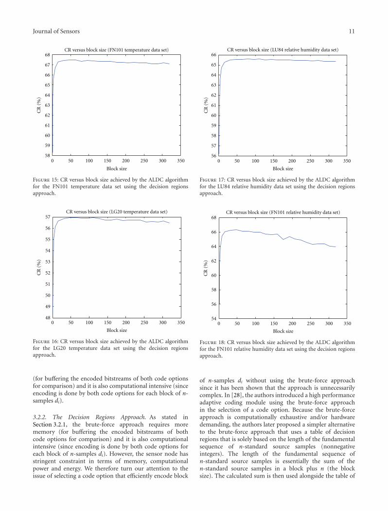
4.2.2. Compression Performance Using the Decision RegionsApproach. The compression performance of our proposedALDC is computed for different value of n and for each ofthe seven data sets using the decision regions approach. Theresults are plotted in Figures 14, 15, 16, 17, 18, 19, and 20.Figures 14 to 20 has the same features and characteristicswith the corresponding plots in Figures 7 to 13. Note that,the range of the compression ratio achievable by ALDC foreach of the seven data sets is a function of the entropyHd (see Table 6 for the entropy of the residual data sets)of the residual signal fed into the encoder. Thus, datasets with low entropy (e.g., LU84 temperature data set)yields high compression ratio, while data sets with highentropy (e.g., LG20 relative humidity data set) yields low

compression ratio. Thus, the data feature that affects morethe compression performance of our proposed algorithm isthe entropy Hd of the residual signal fed into the encoder.This confirms that ALDC is actually an entropy encoder.

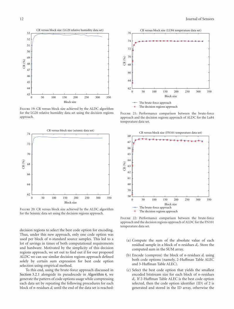
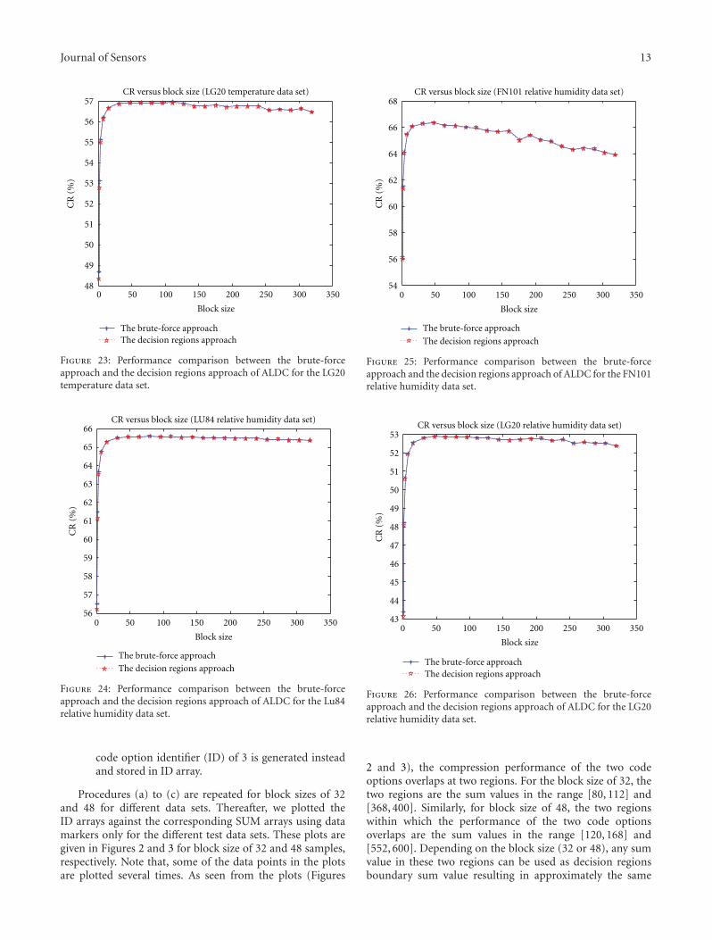
4.2.3. Performance Comparison between the Brute-ForceApproach and the Decision Regions Approach. To ascertainthe correctness and effectiveness of our proposed decisionregion approach method of implementing ALDC, we in thissection compare its compression performances (Figure 14 toFigure 20) with those (Figure 7 to Figure 13) obtained usingthe brute-force approach. For ease of comparison, we plottedthe corresponding figures of all the seven data sets on thesame plot. These plots are shown in Figure 21, 22, 23, 24,25, 26, and 27. From the plots (Figure 21 to Figure 27), itcan be seen that the compression ratio performance achievedby the decision regions approach of ALDC algorithm forthe seven data sets in use is almost the same and for somedata sets same with those obtained using the brute-forceapproach. The slight difference noticed at some points is due


to the overlapping performance of the two code options atand around the two boundary regions. Overall, we can saythat the performance of the decision regions approach isequivalent to that obtained using the brute-force approach.The decision regions approach is computationally morelightweight than the brute-force approach and it requireless resources which makes it suitable for implementation inWSNs. In view of this, we recommend to every user of ourproposed ALDC algorithm to implement only the decisionregions approach. Henceforth, any mention of the ALDCalgorithm in this article should be taken to mean its decisionregions approach.

4.3. Performance Comparison with Other Lossless CompressionSchemes. In this section, we present our simulation resultsthat demonstrate the lossless compression performance andeffectiveness of our proposed ALDC algorithm. The losslesscompression performance of our proposed ALDC algorithmusing the decision regions approach (with block size of32 and 48) and that of other recently proposed losslesscompression algorithms like LEC and S-LZW are given inTable 7 for all the seven real-world data sets. The compres-sion performance that was achieved by the S-LZW algorithmwas adopted from [3] with the following fixed parameters:MINI-CACHE ENTRIES = 32, MAX DICT ENTRIES = 512,BLOCK SIZE = 528 bytes, and DICTIONARY STRATEGY= Frozen [3, 15]. In addition, the lossless compressionperformance achieved by the LEC algorithm and recordedin Table 7 were the result of our simulations of the LECalgorithm following the descriptions in the original papersas closely as possible. It can therefore be seen from Table 7that, our proposed ALDC algorithm outperforms all theother recently proposed lossless compression schemes forWSNs. In addition, a good look at Figure 10 to Figure 16shows that the compression performance of ALDC for blocksize of 1 (i.e., when n = 1) is quite high (just trailingthe performances of LEC) and better than that achieved bythe S-LZW algorithm for all the seven data sets. Similarly,with block size as small as say 4 (i.e., n = 4), the losslesscompression performance achieved by our proposed ALDCalgorithm using the decision regions approach is better thanthat achieved by all the other previously proposed losslesscompression algorithms for all the seven data sets.

Sensor nodes transmit data in packets and many systemsrecommend packet size of not more than 90 bytes. Forexample, the TinyOS operating systems have sets the defaultpacket payload to 29 bytes. We therefore took advantage ofthis inherent sensor node transmission mode by collectingsource samples in a buffer. We encode the samples inthe buffer together. Using the right buffer size (and/orblock size), encoding can be done in real-time. Thus, ourproposed ALDC algorithm has significant advantages overother lossless compression schemes. While other schemes canonly be applied in delay-tolerant applications (e.g., S-LZW)or real-time (delay-intolerant) applications (e.g., LEC), ourproposed ALDC scheme can be applicable in both scenarios.Our proposed scheme achieved compression performanceup to 74.02% for the real-world datasets.

In terms of algorithm complexity, our proposed ALDCalgorithm is simple. When compared to the LEC algorithm,our proposed algorithm requires only slightly more memory.When compared to the S-LZW, our proposed algorithmrequires much less memory.

5. Conclusion

In this paper, we have presented a lightweight adaptivelossless data compression algorithm for wireless sensornetworks. Our proposed ALDC Scheme performs com-pression losslessly using two code options. Our proposedALDC algorithm is efficient and simple, and is particularlysuitable for resource-constrained wireless sensor nodes. Ourproposed ALDC compression scheme allows compressionto dynamically adjust to a changing source. Our proposedalgorithm reduce the data amount for transmission whichcontributes to the energy saving. Additionally, our proposedalgorithm can be used in monitoring systems that havedifferent types of data and still provide satisfactory com-pression ratios. Furthermore, our proposed ALDC algorithmtook into account the different real-time requirements ondata compression. Thus, our algorithm is suitable for bothreal-time and delay-tolerant transmission. Our proposedscheme achieved compression performance up to 74.02%using real-world data sets. We also report and analyze usingreal-world data sets the performance comparisons betweenour proposed ALDC and other recently proposed losslesscompression schemes for WSNs like LEC and S-LZW. Weshowed that our proposed ALDC algorithm outperforms allthe other recently proposed lossless compression schemes.In future, we intend to carry out a formal mathematicalmodeling and analyses of the Decision Regions Approach ofour proposed ALDC algorithm.

References

[1] G. Anastasi, M. Conti, M. Di Francesco, and A. Passarella,“Energy conservation in wireless sensor networks: a survey,”Ad Hoc Networks, vol. 7, no. 3, pp. 537–568, 2009.

[2] N. Kimura and S. Latifi, “A survey on data compression inwireless sensor networks,” in Proceedings of the InternationalConference on Information Technology: Coding and Computing(ITCC ’05), vol. 2, pp. 8–13, April 2005.

[3] F. Marcelloni and M. Vecchio, “An efficient lossless compres-sion algorithm for tiny nodes of monitoring wireless sensornetworks,” Computer Journal, vol. 52, no. 8, pp. 969–987, 2009.

[4] C. Tharini and P. Vanaja Ranjan, “Design of modified adaptiveHuffman data compression algorithm for wireless sensornetwork,” Journal of Computer Science, vol. 5, no. 6, pp. 466–470, 2009.

[5] J. Yick, B. Mukherjee, and D. Ghosal, “Wireless sensor networksurvey,” Computer Networks, vol. 52, no. 12, pp. 2292–2330,2008.

[6] I. F. Akyildiz and M. C. Vuran, Wireless Sensor Networks, JohnWiley & Sons, Chichester, UK, 2010.

[7] C. Tharini and P. V. Ranjan, “An efficient data gatheringscheme for Wireless Sensor Networks,” European Journal ofScientific Research, vol. 43, no. 1, pp. 148–155, 2010.

[8] I. F. Akyildiz, W. Su, Y. Sankarasubramaniam, and E. Cayirci,


“Wireless sensor networks: a survey,” Computer Networks, vol.38, no. 4, pp. 393–422, 2002.

[9] K. Dolfus and T. Braun, “An evaluation of compressionschemes for wireless networks,” in Proceedings of the Inter-national Congress on Ultra Modern Telecommunications andControl Systems and Workshops (ICUMT ’10), pp. 1183–1188,October 2010.

[10] A. van der Byl, R. Neilson, and R. H. Wilkinson, “An evalua-tion of compression techniques for Wireless Sensor Networks,”in Proceedings of the IEEE Africon, pp. 1–6, September 2009.

[11] K. C. Barr and K. Asanovic, “Energy-aware lossless datacompression,” ACM Transactions on Computer Systems, vol. 24,no. 3, pp. 250–291, 2006.

[12] F. Marcelloni and M. Vecchio, “A simple algorithm for datacompression in wireless sensor networks,” IEEE Communica-tions Letters, vol. 12, no. 6, pp. 411–413, 2008.

[13] T. Srisooksai, K. Keamarungsi, P. Lamsrichan, and K. Araki,“Practical data compression in wireless sensor networks: asurvey,” Journal of Network and Computer Applications, vol. 35,no. 1, pp. 37–59, 2012.

[14] T. Schoellhammer, E. Osterweil, B. Greenstein, M. Wimbrow,and D. Estrin, “Lightweight temporal compression of micro-climate datasets,” in Proceedings of the 29th Annual IEEEInternational Conference on Local Computer Networks (LCN’04), pp. 516–524, November 2004.

[15] C. M. Sadler and M. Martonosi, “Data compression algo-rithms for energy-constrained devices in delay tolerant net-works,” in Proceedings of the 4th International Conference onEmbedded Networked Sensor Systems (SenSys ’06), pp. 265–278, November 2006.

[16] S. S. Pradhan, J. Kusuma, and K. Ramchandran, “Distributedcompression in a dense microsensor network,” IEEE SignalProcessing Magazine, vol. 19, no. 2, pp. 51–60, 2002.

[17] J. Chou, D. Petrovic, and K. Ramchandran, “A distributedand adaptive signal processing approach to reducing energyconsumption in sensor networks,” in Proceedings of the22nd Annual Joint Conference on the IEEE Computer andCommunications Societies, pp. 1054–1062, April 2003.

[18] A. Ciancio and A. Ortega, “A distributed wavelet compres-sion algorithm for wireless multihop sensor networks usinglifting,” in Proceedings of the IEEE International Conference onAcoustics, Speech, and Signal Processing (ICASSP ’05), vol. 4,pp. IV825–IV828, March 2005.

[19] A. Ciancio, S. Pattem, A. Ortega, and B. Krishnamachari,“Energy-efficient data representation and routing for wirelesssensor networks based on a distributed wavelet compressionalgorithm,” in Proceedings of the 5th International Conferenceon Information Processing in Sensor Networks (IPSN ’06), pp.309–316, April 2006.

[20] J. J. Xiao, S. Cui, Z. Q. Luo, and A. J. Goldsmith, “Powerscheduling of universal decentralized estimation in sensornetworks,” IEEE Transactions on Signal Processing, vol. 54, no.2, pp. 413–422, 2006.

[21] J. B. Predd, S. R. Kulkarni, and H. V. Poor, “Distributedlearning in wireless sensor networks,” IEEE Signal ProcessingMagazine, vol. 23, no. 4, pp. 56–69, 2006.

[22] D. L. Donoho, “Compressed sensing,” IEEE Transactions onInformation Theory, vol. 52, no. 4, pp. 1289–1306, 2006.

[23] E. P. Capo-Chichi, H. Guyennet, and J. M. Friedt, “K-RLE: anew data compression algorithm for wireless sensor network,”in Proceedings of the 3rd International Conference on SensorTechnologies and Applications, (SENSORCOMM ’09), pp. 502–507, June 2009.

[24] F. Marcelloni and M. Vecchio, “Enabling energy-efficient and

lossy-aware data compression in wireless sensor networksby multi-objective evolutionary optimization,” InformationSciences, vol. 180, no. 10, pp. 1924–1941, 2010.

[25] A. K. Maurya, D. Singh, and A. K. Sarje, “Median predic-tor based data compression algorithm for Wireless SensorNetwork,” International Journal of Smart Sensors and Ad HocNetworks, vol. 1, no. 1, pp. 62–65, 2011.

[26] Y. Liang and W. Peng, “Minimizing energy consumptionsin Wireless Sensor Networks via two-modal transmission,”Computer Communication Review, vol. 40, no. 1, pp. 13–18,2010.

[27] T. A. Welch, “Technique for high-performance data compres-sion,” Computer, vol. 17, no. 6, pp. 8–19, 1984.

[28] R. F. Rice, P. S. Yeh, and W. Miller, “Algorithms for a veryhigh speed universal noiseless coding module,” JPL PublicationLaboratory, vol. 91, no. 1, pp. 1–30, 1991.

[29] “SensorScope deployments homepage,” 2012, http://sensor-scope.epfl.ch/index.php/Main Page.

[30] “TinyNode homepage,” 2012, http://www.tinynode.com/.[31] “Sensirion homepage,” 2012, http://www.sensirion.com/.[32] “Seismic dataset,” 2012, http://www-math.bgsu.edu/?zirbel/.

International Journal of

AerospaceEngineeringHindawi Publishing Corporationhttp://www.hindawi.com Volume 2010

RoboticsJournal of

Hindawi Publishing Corporationhttp://www.hindawi.com Volume 2014


Active and Passive Electronic Components

Control Scienceand Engineering

Journal of



RotatingMachinery


Hindawi Publishing Corporation http://www.hindawi.com

Journal ofEngineeringVolume 2014

Submit your manuscripts athttp://www.hindawi.com

VLSI Design



Shock and Vibration


Civil EngineeringAdvances in

Acoustics and VibrationAdvances in



Electrical and Computer Engineering

Journal of

Advances inOptoElectronics

Hindawi Publishing Corporation http://www.hindawi.com

Volume 2014

The Scientific World JournalHindawi Publishing Corporation http://www.hindawi.com Volume 2014

SensorsJournal of


Modelling & Simulation in EngineeringHindawi Publishing Corporation http://www.hindawi.com Volume 2014


Chemical EngineeringInternational Journal of Antennas and

Propagation




Navigation and Observation



DistributedSensor Networks


AnAdaptiveLosslessDataCompressionSchemefor ... · This is an open access article distributed under...

Documents

Transcript of AnAdaptiveLosslessDataCompressionSchemefor ... · This is an open access article distributed under...