AN4841 Application note · AN4841 Rev 2 3/25 AN4841 List of tables 3 List of tables Table 1. Pros...

February 2018 AN4841 Rev 2 1/25

1

AN4841Application note

Digital signal processing for STM32 microcontrollers using CMSIS

Introduction

This application note describes the development of digital filters for analog signals, and the transformations between time and frequency domains. The examples discussed in this document include a low-pass and a high-pass FIR filter, as well as Fourier fast transforms with floating and fixed point at different frequencies.

The associated firmware (X-CUBE-DSPDEMO), applicable to STM32F429xx and STM32F746xx MCUs, can be adapted to any STM32 microcontroller.

Digital Signal Processing (DSP) is the mathematical manipulation and processing of signals. Signals to be processed come in various physical formats that include audio, video or any analog signal that carries information, such as the output signal of a microphone.

Both Cortex®-M4-based STM32F4 Series and Cortex®-M7-based STM32F7 Series provide instructions for signal processing, and support advanced SIMD (Single Instruction Multi Data) and Single cycle MAC (Multiply and Accumulate) instructions.

The use of STM32 MCUs in a real-time DSP application not only reduces cost, but also reduces the overall power consumption.

The following documents are considered as references:

• PM0214, “STM32F3 and STM32F4 Series Cortex®-M4 programming manual”, available on www.st.com

• PM0253, “STM32F7 Series Cortex®-M7 programming manual”, available on www.st.com

• CMSIS - Cortex® Microcontroller Software Interface Standard, available on www.arm.com

• Arm® compiler toolchain Compiler reference, available on http://infocenter.arm.com

• “Developing Optimized Signal Processing Software on the Cortex®-M4 Processor”, technical paper by Shyam Sadasivan, available on www.techonline.com.

www.st.com

http://www.st.com

Contents AN4841

2/25 AN4841 Rev 2

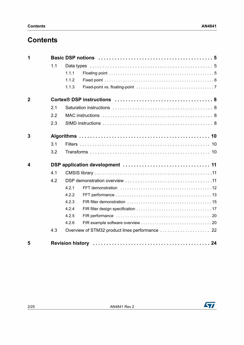
Contents

1 Basic DSP notions . . . . . . . . . . . . . . . . . . . . . . . . . . . . . . . . . . . . . . . . . . 5

1.1 Data types . . . . . . . . . . . . . . . . . . . . . . . . . . . . . . . . . . . . . . . . . . . . . . . . . 5

1.1.1 Floating point . . . . . . . . . . . . . . . . . . . . . . . . . . . . . . . . . . . . . . . . . . . . . . 5

1.1.2 Fixed point . . . . . . . . . . . . . . . . . . . . . . . . . . . . . . . . . . . . . . . . . . . . . . . . 6

1.1.3 Fixed-point vs. floating-point . . . . . . . . . . . . . . . . . . . . . . . . . . . . . . . . . . 7

2 Cortex® DSP instructions . . . . . . . . . . . . . . . . . . . . . . . . . . . . . . . . . . . . 8

2.1 Saturation instructions . . . . . . . . . . . . . . . . . . . . . . . . . . . . . . . . . . . . . . . . 8

2.2 MAC instructions . . . . . . . . . . . . . . . . . . . . . . . . . . . . . . . . . . . . . . . . . . . . 8

2.3 SIMD instructions . . . . . . . . . . . . . . . . . . . . . . . . . . . . . . . . . . . . . . . . . . . . 8

3 Algorithms . . . . . . . . . . . . . . . . . . . . . . . . . . . . . . . . . . . . . . . . . . . . . . . . 10

3.1 Filters . . . . . . . . . . . . . . . . . . . . . . . . . . . . . . . . . . . . . . . . . . . . . . . . . . . . 10

3.2 Transforms . . . . . . . . . . . . . . . . . . . . . . . . . . . . . . . . . . . . . . . . . . . . . . . . 10

4 DSP application development . . . . . . . . . . . . . . . . . . . . . . . . . . . . . . . . 11

4.1 CMSIS library . . . . . . . . . . . . . . . . . . . . . . . . . . . . . . . . . . . . . . . . . . . . . . .11

4.2 DSP demonstration overview . . . . . . . . . . . . . . . . . . . . . . . . . . . . . . . . . . .11

4.2.1 FFT demonstration . . . . . . . . . . . . . . . . . . . . . . . . . . . . . . . . . . . . . . . . 12

4.2.2 FFT performance . . . . . . . . . . . . . . . . . . . . . . . . . . . . . . . . . . . . . . . . . . 13

4.2.3 FIR filter demonstration . . . . . . . . . . . . . . . . . . . . . . . . . . . . . . . . . . . . . 15

4.2.4 FIR filter design specification . . . . . . . . . . . . . . . . . . . . . . . . . . . . . . . . . 17

4.2.5 FIR performance . . . . . . . . . . . . . . . . . . . . . . . . . . . . . . . . . . . . . . . . . . 20

4.2.6 FIR example software overview . . . . . . . . . . . . . . . . . . . . . . . . . . . . . . . 20

4.3 Overview of STM32 product lines performance . . . . . . . . . . . . . . . . . . . . 22

5 Revision history . . . . . . . . . . . . . . . . . . . . . . . . . . . . . . . . . . . . . . . . . . . 24

AN4841 Rev 2 3/25

AN4841 List of tables

3

List of tables

Table 1. Pros and cons of number formats in DSP applications . . . . . . . . . . . . . . . . . . . . . . . . . . . . 7Table 2. Saturating instructions . . . . . . . . . . . . . . . . . . . . . . . . . . . . . . . . . . . . . . . . . . . . . . . . . . . . . 8Table 3. SIMD instructions . . . . . . . . . . . . . . . . . . . . . . . . . . . . . . . . . . . . . . . . . . . . . . . . . . . . . . . . . 9Table 4. FIR filter specifications . . . . . . . . . . . . . . . . . . . . . . . . . . . . . . . . . . . . . . . . . . . . . . . . . . . . 17Table 5. FFT performance . . . . . . . . . . . . . . . . . . . . . . . . . . . . . . . . . . . . . . . . . . . . . . . . . . . . . . . . 23Table 6. Revision history . . . . . . . . . . . . . . . . . . . . . . . . . . . . . . . . . . . . . . . . . . . . . . . . . . . . . . . . . 24

List of figures AN4841

4/25 AN4841 Rev 2

List of figures

Figure 1. Single precision number format . . . . . . . . . . . . . . . . . . . . . . . . . . . . . . . . . . . . . . . . . . . . . . 5Figure 2. Double precision number format. . . . . . . . . . . . . . . . . . . . . . . . . . . . . . . . . . . . . . . . . . . . . . 5Figure 3. 32 bits fixed point number format . . . . . . . . . . . . . . . . . . . . . . . . . . . . . . . . . . . . . . . . . . . . . 6Figure 4. FFT size calculation performance on STM32F429. . . . . . . . . . . . . . . . . . . . . . . . . . . . . . . 13Figure 5. FFT size calculation performance on STM32F746. . . . . . . . . . . . . . . . . . . . . . . . . . . . . . . 13Figure 6. Running FFT 1024 points with input data in Float-32 on STM32F429I-DISCO . . . . . . . . . 14Figure 7. Running FFT 1024 points with input data in Float-32 on STM32F746-DISCO. . . . . . . . . . 15Figure 8. Block diagram of the FIR example . . . . . . . . . . . . . . . . . . . . . . . . . . . . . . . . . . . . . . . . . . . 15Figure 9. Generated input (sum of two sine waves) . . . . . . . . . . . . . . . . . . . . . . . . . . . . . . . . . . . . . 16Figure 10. Magnitude spectrum of the input signal . . . . . . . . . . . . . . . . . . . . . . . . . . . . . . . . . . . . . . . 17Figure 11. FIR filter verification using MATLAB® FVT tool . . . . . . . . . . . . . . . . . . . . . . . . . . . . . . . . . 19Figure 12. FIR filter computation performance for STM32F429. . . . . . . . . . . . . . . . . . . . . . . . . . . . . . 20Figure 13. FIR filter computation performance for STM32F746. . . . . . . . . . . . . . . . . . . . . . . . . . . . . . 20Figure 14. FIR demonstration results on STM32F429I-DISCO . . . . . . . . . . . . . . . . . . . . . . . . . . . . . . 21Figure 15. FIR demonstration results on STM32F746-DISCO . . . . . . . . . . . . . . . . . . . . . . . . . . . . . . 21

AN4841 Rev 2 5/25

AN4841 Basic DSP notions

24

1 Basic DSP notions

1.1 Data types

DSP operations can use either floating-point or fixed-point formats.

1.1.1 Floating point

Floating point is a method to represent real numbers.

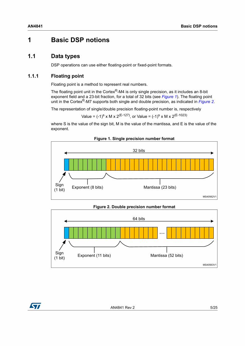
The floating point unit in the Cortex®-M4 is only single precision, as it includes an 8-bit exponent field and a 23-bit fraction, for a total of 32 bits (see Figure 1). The floating point unit in the Cortex®-M7 supports both single and double precision, as indicated in Figure 2.

The representation of single/double precision floating-point number is, respectively

Value = (-1)s x M x 2(E-127), or Value = (-1)s x M x 2(E-1023)

where S is the value of the sign bit, M is the value of the mantissa, and E is the value of the exponent.

Figure 1. Single precision number format

Figure 2. Double precision number format

Basic DSP notions AN4841

6/25 AN4841 Rev 2

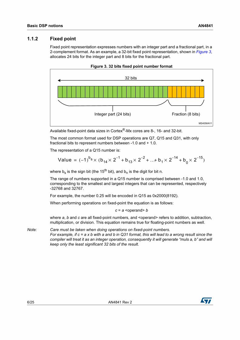
1.1.2 Fixed point

Fixed point representation expresses numbers with an integer part and a fractional part, in a 2-complement format. As an example, a 32-bit fixed point representation, shown in Figure 3, allocates 24 bits for the integer part and 8 bits for the fractional part.

Figure 3. 32 bits fixed point number format

Available fixed-point data sizes in Cortex®-Mx cores are 8-, 16- and 32-bit.

The most common format used for DSP operations are Q7, Q15 and Q31, with only fractional bits to represent numbers between -1.0 and + 1.0.

The representation of a Q15 number is:

Value 1–( )bs b14 21–× b13 2

2–× … b1 214–× b

02

15–×+ + + +( )×=

where bs is the sign bit (the 15th bit), and bn is the digit for bit n.

The range of numbers supported in a Q15 number is comprised between -1.0 and 1.0, corresponding to the smallest and largest integers that can be represented, respectively -32768 and 32767.

For example, the number 0.25 will be encoded in Q15 as 0x2000(8192).

When performing operations on fixed-point the equation is as follows:

c = a <operand> b

where a, b and c are all fixed-point numbers, and <operand> refers to addition, subtraction, multiplication, or division. This equation remains true for floating-point numbers as well.

Note: Care must be taken when doing operations on fixed-point numbers. For example, if c = a x b with a and b in Q31 format, this will lead to a wrong result since the compiler will treat it as an integer operation, consequently it will generate “muls a, b” and will keep only the least significant 32 bits of the result.

AN4841 Rev 2 7/25

AN4841 Basic DSP notions

24

1.1.3 Fixed-point vs. floating-point

Table 1 highlights the main advantages and disadvantages of fixed-point vs. floating-point in DSP applications.

Table 1. Pros and cons of number formats in DSP applications

Number format Fixed point Floating point

Advantages Fast implementation Supports a much wider range of values

DisadvantagesLimited number range

Can easily go in overflowNeeds more memory space

Cortex® DSP instructions AN4841

8/25 AN4841 Rev 2

2 Cortex® DSP instructions

The Cortex®-Mx cores feature several instructions that result in efficient implementation of DSP algorithms.

2.1 Saturation instructions

Saturating, addition and subtraction instructions are available for 8-, 16- and 32-bit values, some of these instructions are listed in Table 2.

The SSAT (Signed SATurate) instruction is used to scale and saturate a signed value to any bit position, with optional shift before saturating.

2.2 MAC instructions

Multiply ACcumulate (MAC) instructions are widely used in DSP algorithms, as in the case of the Finite Impulse Response (FIR) and Infinite Impulse Response (IIR).

Executing multiplication and accumulation in single cycle instruction is a key requirement for achieving high performance.

The following example explains how the SMMLA (Signed Most significant word MuLtiply Accumulate) instruction works.

2.3 SIMD instructions

In addition to MAC instructions that execute a multiplication and an accumulation in a single cycle, there are the SIMD (Single Instruction Multiple Data) instructions, performing multiple identical operations in a single cycle instruction.

Table 2. Saturating instructions

Code Function

QADD8 Saturating four 8-bit integer additions

QSUB8 Saturating four 8-bit integer subtraction

QADD16 Saturating two 16-bit integer additions

QSUB16 Saturating two 16-bit integer subtraction

QADD Saturating 32-bit add

QSUB Saturating 32-bit subtraction

AN4841 Rev 2 9/25

AN4841 Cortex® DSP instructions

24

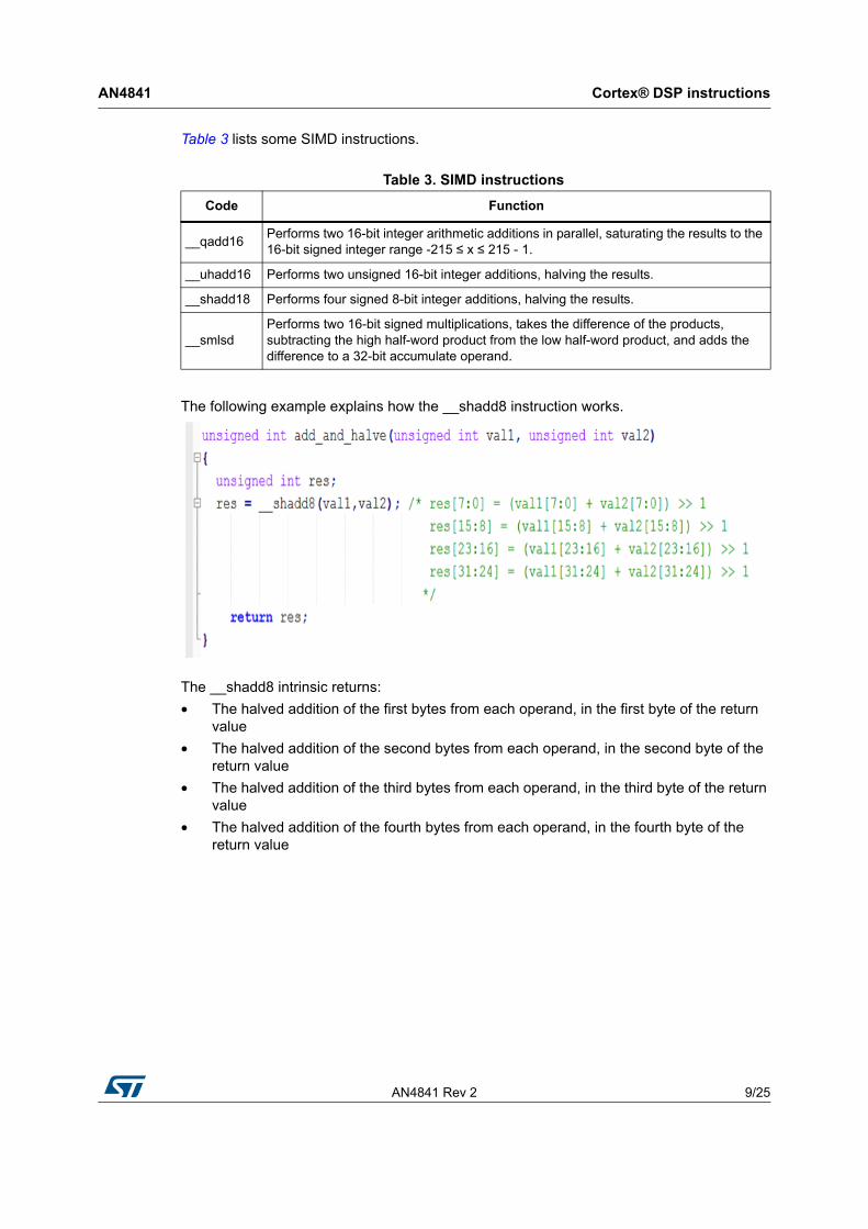
Table 3 lists some SIMD instructions.

The following example explains how the __shadd8 instruction works.

The __shadd8 intrinsic returns:

• The halved addition of the first bytes from each operand, in the first byte of the return value

• The halved addition of the second bytes from each operand, in the second byte of the return value

• The halved addition of the third bytes from each operand, in the third byte of the return value

• The halved addition of the fourth bytes from each operand, in the fourth byte of the return value

Table 3. SIMD instructions

Code Function

__qadd16Performs two 16-bit integer arithmetic additions in parallel, saturating the results to the 16-bit signed integer range -215 ≤ x ≤ 215 - 1.

__uhadd16 Performs two unsigned 16-bit integer additions, halving the results.

__shadd18 Performs four signed 8-bit integer additions, halving the results.

__smlsdPerforms two 16-bit signed multiplications, takes the difference of the products, subtracting the high half-word product from the low half-word product, and adds the difference to a 32-bit accumulate operand.

Algorithms AN4841

10/25 AN4841 Rev 2

3 Algorithms

3.1 Filters

The most common digital filters are:

• FIR (Finite Impulse Response): used, among others, in motor control and audio equalization

• IIR (Infinite Impulse Response): used in smoothing data

The IIR filter can be used to implement filters such as Butterworth, Chebyshev, and Bessel.

3.2 Transforms

A transform is a function that converts data from a domain into another.

The FFT (Fast Fourier Transform) is a typical example: it is an efficient algorithm used to convert a discrete time-domain signal into an equivalent frequency-domain signal based on the Discrete Fourier Transform (DFT).

AN4841 Rev 2 11/25

AN4841 DSP application development

24

4 DSP application development

4.1 CMSIS library

The Arm® Cortex® Microcontroller Software Interface Standard (CMSIS) is a vendor-independent hardware abstraction layer for all Cortex® processor based devices.

CMSIS has been developed by Arm® in conjunction with silicon, tools and middleware partners.

The idea behind CMSIS is to provide a consistent and simple software interface to the processor for interface peripherals, real-time operating systems, and middleware, simplifying software re -use, reducing the learning curve for new microcontroller developments and reducing the time to market for new devices.

CMSIS library comes with ST firmware under \Drivers\CMSIS\.

The CMSIS-DSP library includes:

• Basic mathematical functions with vector operations

• Fast mathematical functions, like sine and cosine

• Complex mathematical functions like calculating magnitude

• Filtering functions like FIR or IIR

• Matrix computing functions

• Transform functions like FFT

• Controller functions like PID controller

• Statistical functions like calculating minimum or maximum

• Support functions like converting from one format to another

• Interpolation functions

Most algorithms uses floating-point and fixed-point in various formats. For example, in FIR case, the available Arm® functions are:

• arm_fir_init_f32

• arm_fir_f32

• arm_fir_init_q31

• arm_fir_q31

• arm_fir_fast_q31

• arm_fir_init_q15

• arm_fir_q15

• arm_fir_fast_q15

• arm_fir_init_q7

• arm_fir_q7

4.2 DSP demonstration overview

The goal of this demonstration is to show a full integration with STM32F429 using ADC, DAC, DMA and timers, and also calling CMSIS routines, all with the use of graphics, taking advantage of the 2.4" QVGA TFT LCD included in the discovery board.

DSP application development AN4841

12/25 AN4841 Rev 2

This demonstration also shows how easy it is to migrate an application from an STM32F4 microcontroller to one of the STM32F7 Series.

A graphical user interface is designed using STemWin, to simplify access to different features of the demonstration.

4.2.1 FFT demonstration

The main features of this FFT example are

• For the STM32F429

– Generate data signal and transfer it through DMA1 Stream6 Channel7 to DAC output Channel2

– Acquire data signal with ADC Channel0 and transfer it for elaboration through DMA2 Stream0 Channel0

– Vary the frequency of the input signal using Timer 2

– Initialize FFT processing with various data: Float-32, Q15 and Q31

– Perform FFT processing and calculate the magnitude values

– Draw input and output data on LCD screen

• For the STM32F746

– Generate data signal and transfer it through DMA1 Stream5 Channel7 to DAC output Channel1

– Acquire data signal with ADC Channel4 and transfer it for elaboration through DMA2 Stream0 Channel0

– Vary the frequency of the input signal using Timer 2

– Initialize FFT processing with various data: Float-32, Q15 and Q31

– Perform FFT processing and calculate the magnitude values

– Draw input and output data on LCD screen

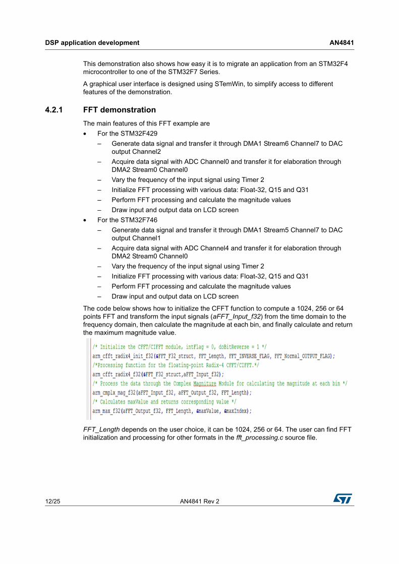
The code below shows how to initialize the CFFT function to compute a 1024, 256 or 64 points FFT and transform the input signals (aFFT_Input_f32) from the time domain to the frequency domain, then calculate the magnitude at each bin, and finally calculate and return the maximum magnitude value.

FFT_Length depends on the user choice, it can be 1024, 256 or 64. The user can find FFT initialization and processing for other formats in the fft_processing.c source file.

AN4841 Rev 2 13/25


24

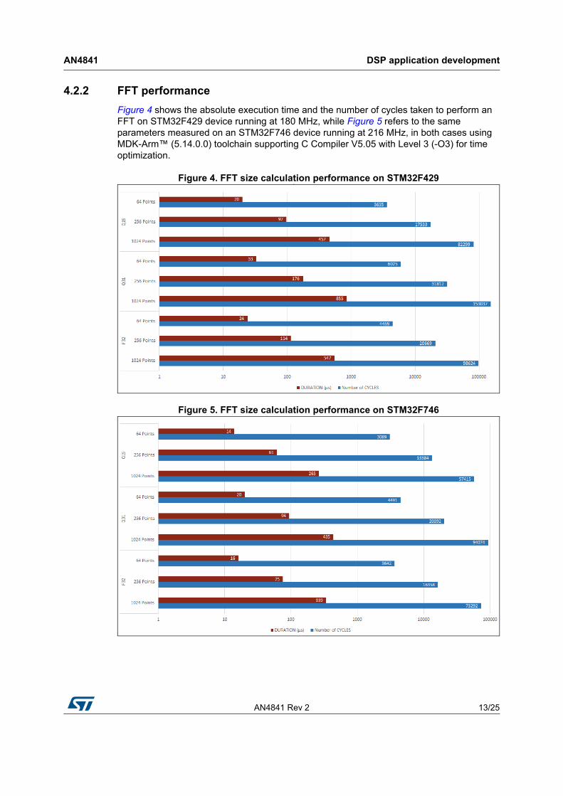
4.2.2 FFT performance

Figure 4 shows the absolute execution time and the number of cycles taken to perform an FFT on STM32F429 device running at 180 MHz, while Figure 5 refers to the same parameters measured on an STM32F746 device running at 216 MHz, in both cases using MDK-Arm™ (5.14.0.0) toolchain supporting C Compiler V5.05 with Level 3 (-O3) for time optimization.

Figure 4. FFT size calculation performance on STM32F429

Figure 5. FFT size calculation performance on STM32F746


14/25 AN4841 Rev 2

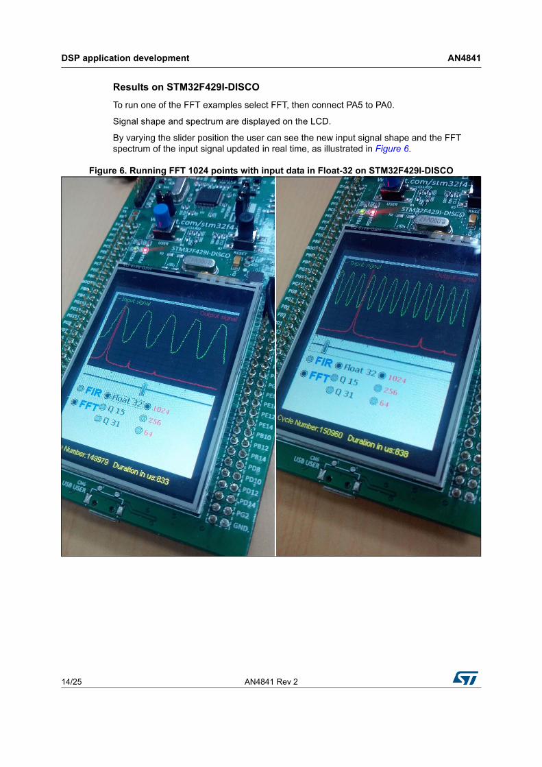
Results on STM32F429I-DISCO

To run one of the FFT examples select FFT, then connect PA5 to PA0.

Signal shape and spectrum are displayed on the LCD.

By varying the slider position the user can see the new input signal shape and the FFT spectrum of the input signal updated in real time, as illustrated in Figure 6.

Figure 6. Running FFT 1024 points with input data in Float-32 on STM32F429I-DISCO

AN4841 Rev 2 15/25


24

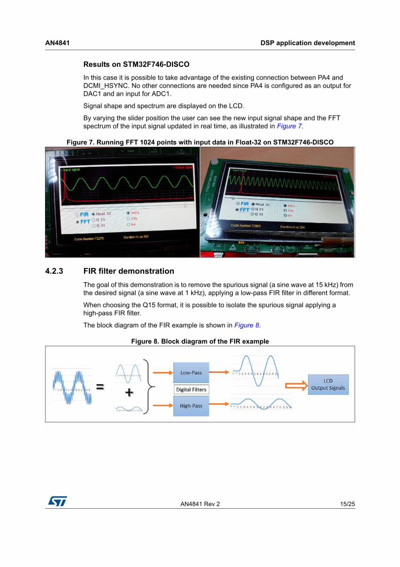
Results on STM32F746-DISCO

In this case it is possible to take advantage of the existing connection between PA4 and DCMI_HSYNC. No other connections are needed since PA4 is configured as an output for DAC1 and an input for ADC1.

Signal shape and spectrum are displayed on the LCD.

By varying the slider position the user can see the new input signal shape and the FFT spectrum of the input signal updated in real time, as illustrated in Figure 7.

Figure 7. Running FFT 1024 points with input data in Float-32 on STM32F746-DISCO

4.2.3 FIR filter demonstration

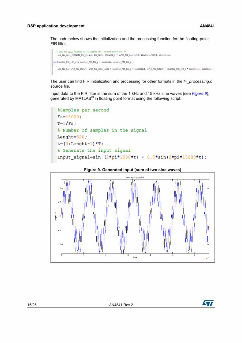
The goal of this demonstration is to remove the spurious signal (a sine wave at 15 kHz) from the desired signal (a sine wave at 1 kHz), applying a low-pass FIR filter in different format.

When choosing the Q15 format, it is possible to isolate the spurious signal applying a high-pass FIR filter.

The block diagram of the FIR example is shown in Figure 8.

Figure 8. Block diagram of the FIR example


16/25 AN4841 Rev 2

The code below shows the initialization and the processing function for the floating-point FIR filter.

The user can find FIR initialization and processing for other formats in the fir_processing.c source file.

Input data to the FIR filter is the sum of the 1 kHz and 15 kHz sine waves (see Figure 9), generated by MATLAB® in floating point format using the following script:

Figure 9. Generated input (sum of two sine waves)

AN4841 Rev 2 17/25


24

The magnitude spectrum of the input signal (Figure 10) shows that there are two frequencies, 1 kHz and 15 kHz.

Figure 10. Magnitude spectrum of the input signal

As the noise is positioned around 15 kHz, the cutoff point must be set at a lower frequency, namely at 6 kHz.

4.2.4 FIR filter design specification

The main features are listed in Table 4.

Table 4. FIR filter specifications

Feature / Parameter Value

Type Low-pass

Order 28

Sampling frequency 48 kHz

Cut-off frequency 6 kHz


18/25 AN4841 Rev 2

The low-pass filter is designed with MATLAB®, using the commands shown below

Note: FIR filter order is equal to the number of coefficients -1.

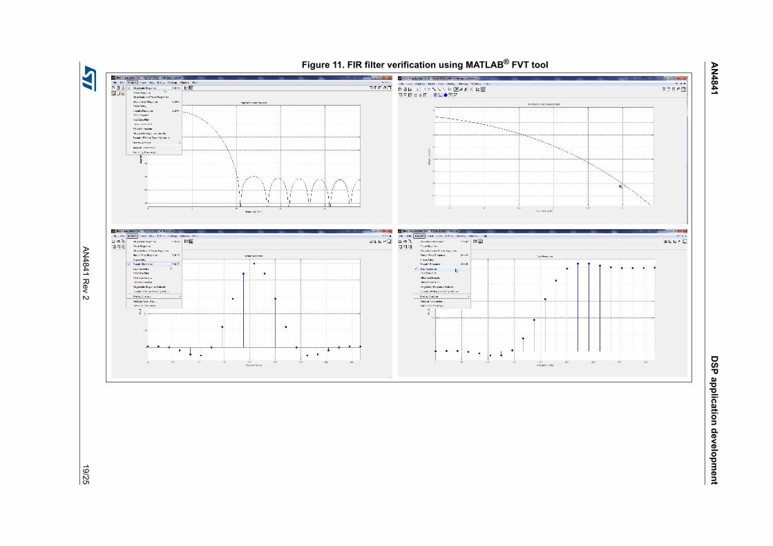
In order to verify the designed filter, it’s possible to use the Filter Visualization Tool in MATLAB® using the following command:

The Filter Visualization Tool (FVT) is a practical tool allowing the user to verify the details and the parameters of the built filter.

In Figure 11 are reported (left to right, top to bottom):

• magnitude response

• filter gain (in dB) vs. frequency (in Hz)

• impulse response

• step response

AN

484

1D

SP

app

lica

tion

de

velo

pm

ent

AN

4841 R

ev 219

/25

Figure 11. FIR filter verification using MATLAB® FVT tool


20/25 AN4841 Rev 2

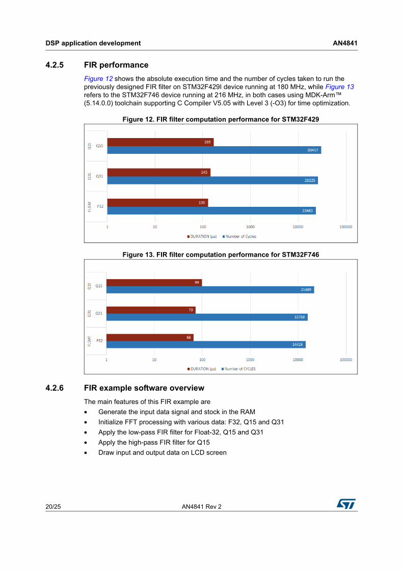
4.2.5 FIR performance

Figure 12 shows the absolute execution time and the number of cycles taken to run the previously designed FIR filter on STM32F429I device running at 180 MHz, while Figure 13 refers to the STM32F746 device running at 216 MHz, in both cases using MDK-Arm™ (5.14.0.0) toolchain supporting C Compiler V5.05 with Level 3 (-O3) for time optimization.

Figure 12. FIR filter computation performance for STM32F429

Figure 13. FIR filter computation performance for STM32F746

4.2.6 FIR example software overview

The main features of this FIR example are

• Generate the input data signal and stock in the RAM

• Initialize FFT processing with various data: F32, Q15 and Q31

• Apply the low-pass FIR filter for Float-32, Q15 and Q31

• Apply the high-pass FIR filter for Q15

• Draw input and output data on LCD screen

AN4841 Rev 2 21/25


24

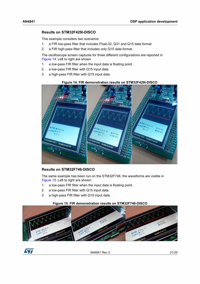
Results on STM32F429I-DISCO

This example considers two scenarios:

1. a FIR low-pass filter that includes Float-32, Q31 and Q15 data format

2. a FIR high-pass filter that includes only Q15 data format.

The oscilloscope screen captures for three different configurations are reported in Figure 14. Left to right are shown

1. a low-pass FIR filter when the input data is floating point

2. a low-pass FIR filter with Q15 input data

3. a high-pass FIR filter with Q15 input data

Figure 14. FIR demonstration results on STM32F429I-DISCO

Results on STM32F746-DISCO

The same example has been run on the STM32F746, the waveforms are visible in Figure 15. Left to right are shown:

1. a low-pass FIR filter when the input data is floating point.

2. a low-pass FIR filter with Q15 input data.

3. a high-pass FIR filter with Q15 input data.

Figure 15. FIR demonstration results on STM32F746-DISCO


22/25 AN4841 Rev 2

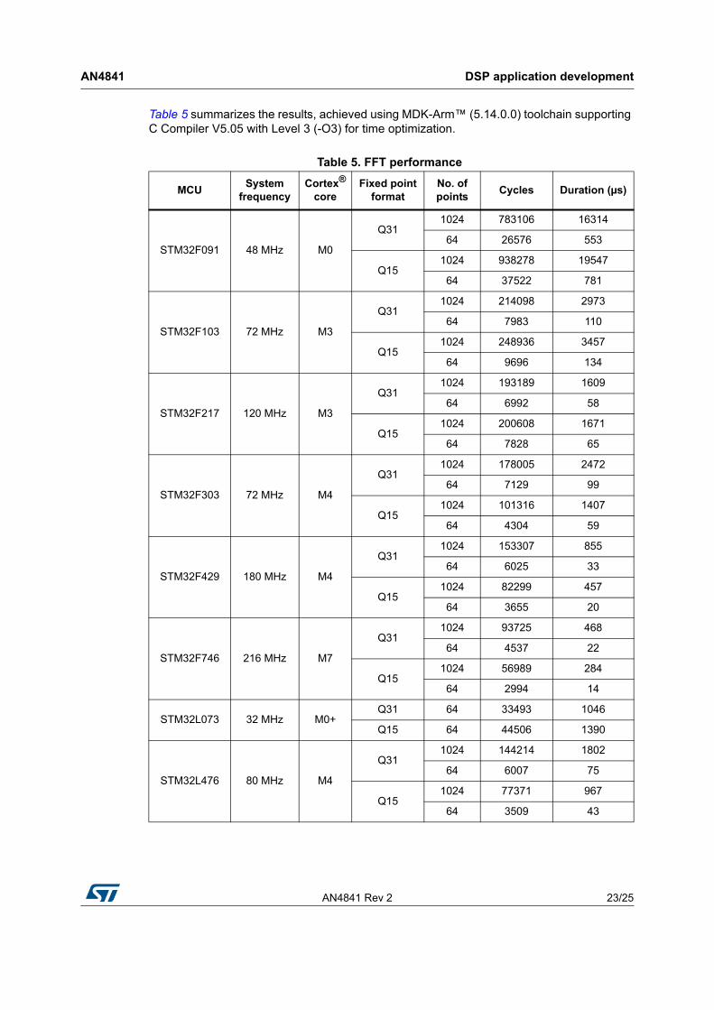
4.3 Overview of STM32 product lines performance

One of the purposes of this application note is to provide benchmarking results for different STM32 Series. In the case in discussion, the DSP algorithm to use are:

• complex FFT using 64 and 1024 points (radix-4)

• use of fixed point format (Q15 and Q31)

The comparison is based on execution time (i.e. the time required for the FFT processing).

The input vector is generated with MATLAB®, using the commands below:

AN4841 Rev 2 23/25


24

Table 5 summarizes the results, achieved using MDK-Arm™ (5.14.0.0) toolchain supporting C Compiler V5.05 with Level 3 (-O3) for time optimization.

Table 5. FFT performance

MCUSystem

frequencyCortex®

coreFixed point

formatNo. of points

Cycles Duration (µs)

STM32F091 48 MHz M0

Q311024 783106 16314

64 26576 553

Q151024 938278 19547

64 37522 781

STM32F103 72 MHz M3

Q311024 214098 2973

64 7983 110

Q151024 248936 3457

64 9696 134

STM32F217 120 MHz M3

Q311024 193189 1609

64 6992 58

Q151024 200608 1671

64 7828 65

STM32F303 72 MHz M4

Q311024 178005 2472

64 7129 99

Q151024 101316 1407

64 4304 59


Q311024 153307 855

64 6025 33

Q151024 82299 457

64 3655 20


Q311024 93725 468

64 4537 22

Q151024 56989 284

64 2994 14

STM32L073 32 MHz M0+Q31 64 33493 1046

Q15 64 44506 1390

STM32L476 80 MHz M4

Q311024 144214 1802

64 6007 75

Q151024 77371 967

64 3509 43

Revision history AN4841

24/25 AN4841 Rev 2

5 Revision history

Table 6. Revision history

Date Revision Description of changes

23-Mar-2016 1 Initial release

23-Feb-2018 2Updated Table 5: FFT performance.

Minor text edits across the whole document.

AN4841 Rev 2 25/25

AN4841

25

IMPORTANT NOTICE – PLEASE READ CAREFULLY

STMicroelectronics NV and its subsidiaries (“ST”) reserve the right to make changes, corrections, enhancements, modifications, and improvements to ST products and/or to this document at any time without notice. Purchasers should obtain the latest relevant information on ST products before placing orders. ST products are sold pursuant to ST’s terms and conditions of sale in place at the time of order acknowledgement.

Purchasers are solely responsible for the choice, selection, and use of ST products and ST assumes no liability for application assistance or the design of Purchasers’ products.

No license, express or implied, to any intellectual property right is granted by ST herein.

Resale of ST products with provisions different from the information set forth herein shall void any warranty granted by ST for such product.

ST and the ST logo are trademarks of ST. All other product or service names are the property of their respective owners.

Information in this document supersedes and replaces information previously supplied in any prior versions of this document.

© 2018 STMicroelectronics – All rights reserved

AN4841 Application note · AN4841 Rev 2 3/25 AN4841 List of tables 3 List of tables Table 1. Pros...

Documents

Transcript of AN4841 Application note · AN4841 Rev 2 3/25 AN4841 List of tables 3 List of tables Table 1. Pros...