An Investigation into the Interactions between Speaker...

An Investigation into the Interactions betweenSpeaker Diarisation Systems andAutomatic Speech Transcription

†S.E. Tranter, †K. Yu, ‡D.A. Reynolds, †G. Evermann,†D.Y. Kim & †P.C. WoodlandCUED/F-INFENG/TR-464

9th October 2003

† Cambridge University Engineering Department ‡MIT-Lincoln LabsTrumpington Street 244 Wood StreetCambridge, CB2 1PZ Lexington, MA 02420-9185England USA{sej28,ky219,ge204,dyk21,pcw }@eng.cam.ac.uk [email protected]

CONTENTS

1 Introduction 1

2 Diarisation 22.1 What is Diarisation . . . . . . . . . . . . . . . . . . . . . . . . . . . . . . . . . . . . . . . . 22.2 Diarisation Scoring . . . . . . . . . . . . . . . . . . . . . . . . . . . . . . . . . . . . . . . . 42.3 The CUED RT-03s CTS Diarisation System . . . . . . . . . . . . . . . . . . . . . . . . . . 62.4 The CUED RT-03s BN Diarisation System . . . . . . . . . . . . . . . . . . . . . . . . . . . 72.5 The MIT-LL RT-03s BN Diarisation System . . . . . . . . . . . . . . . . . . . . . . . . . . 13

3 Speech To Text Systems 163.1 The CTS RT-02 10xRT STT System . . . . . . . . . . . . . . . . . . . . . . . . . . . . . . . 163.2 The BN RT-03 10xRT STT System . . . . . . . . . . . . . . . . . . . . . . . . . . . . . . . . 17

4 CTS Experiments 184.1 How should Diarisation Output be used for STT ? . . . . . . . . . . . . . . . . . . . . . . 184.2 The Relationship between Segmentations and WER . . . . . . . . . . . . . . . . . . . . . 194.3 The Correlation between Diarisation Score and WER . . . . . . . . . . . . . . . . . . . . 204.4 Can Diarisation Scores be Improved Using Information from STT ? . . . . . . . . . . . . 224.5 Variation in Reference Generation . . . . . . . . . . . . . . . . . . . . . . . . . . . . . . . . 234.6 Using Different Sites’ STT segmentations . . . . . . . . . . . . . . . . . . . . . . . . . . . 244.7 Summary of Key Results . . . . . . . . . . . . . . . . . . . . . . . . . . . . . . . . . . . . . 27

5 BN Experiments 285.1 Are Diarisation Scores Correlated with WER ? . . . . . . . . . . . . . . . . . . . . . . . . 285.2 The Effect of Removing Adverts . . . . . . . . . . . . . . . . . . . . . . . . . . . . . . . . 295.3 Can we use Diarisation Output for STT ? . . . . . . . . . . . . . . . . . . . . . . . . . . . 315.4 Using Different Sites’ STT segmentations . . . . . . . . . . . . . . . . . . . . . . . . . . . 325.5 The Effect of Automating Segmentation and Clustering on STT Performance . . . . . . . 325.6 Potential for Improving the Diarisation Score . . . . . . . . . . . . . . . . . . . . . . . . . 335.7 Summary of Key Results . . . . . . . . . . . . . . . . . . . . . . . . . . . . . . . . . . . . . 35

6 Cross-Site Diarisation Experiments 376.1 ’Plug and Play’ Diarisation Systems . . . . . . . . . . . . . . . . . . . . . . . . . . . . . . 38

7 Conclusions 42

8 Acknowledgements 43

A Data 43A.1 Broadcast News Data . . . . . . . . . . . . . . . . . . . . . . . . . . . . . . . . . . . . . . . 43A.2 CTS Data . . . . . . . . . . . . . . . . . . . . . . . . . . . . . . . . . . . . . . . . . . . . . . 44

B Accuracy of CTS Forced Alignments 44

References 46

ABBREVIATIONS USED

Ad Advert(isement) i.e. a commercial in a broadcast news showBIC Bayesian Information CriterionBN Broadcast NewsClust Clustering or ClustererCTS Conversational Telephone SpeechCUED Cambridge University Engineering DepartmentDel Deletion component of word error rate (%)DIARY Total Diarisation score = MS + FA + SPE (%)[ D/I/S] WER broken down by Deletion, Insertion and SubstitutionFA False Alarm component of diarisation score (%)GE Gender Error (%) = confusability between male/female speakersHLDA Heteroscedastic Linear Discriminant AnalysisIns Insertion component of word error rate (%)MFCC Mel-Frequency Cepstral CoefficientsMIT-LL MIT - Lincoln LabsMLE Maximum Likelihood EstimationMLLR Maximum Likelihood Linear RegressionMPE Minimum Phone ErrorMS Missed Speech component of diarisation score (%)PLP Perceptual Linear PredictionSAD Speech Activity DetectionSPE SPeaker Error component of diarisation score (%)STT Speech-To-Text transcriptionSeg Segmentation or SegmenterSub Substitution component of word error rate (%)VTLN Vocal Tract Length NormalisationWER Word Error Rate = Del + Ins + Sub (%)

ctseval02 RT-02 English CTS eval datactsdry03 RT-03 English CTS dryrun data subset of ctseval02ctseval03 RT-03s English CTS STT evaluation datactseval03s The subset of ctseval03 used in the RT-03s English CTS diarisation eval.ctsdev03f The subset of ctseval03 data not in ctseval03s

bnrt02 RT-02 English BN eval data (which is also the BN dryrun data)bndidev03 RT-03s English BN diarisation development databndev03 RT-03 development data defined by STT sitesbneval03 RT-03s English BN STT evaluation databneval03s The subset of bneval03 used in the RT-03s English BN diarisation eval.bndev03f The subset of bneval03 data not in bneval03s

1 Introduction 1

1 INTRODUCTION

Recent years have seen great improvements in the performance of systems to automatically recognisespeech. These ’Speech-to-Text’ (STT) systems can now produce transcriptions of sufficient quality toenable some important tasks, such as information retrieval, to be performed at the same standards asif manual transcriptions were available. (Garofolo, Auzanne and Voorhees 2000, Garofolo, Lard andVoorhees 2001). Research is now focusing on making the transcripts more readable. This still includesdriving down the word error rate (WER), but also encompasses augmenting the automatic transcrip-tion with so-called ’metadata’ information which could be used to help a potential reader in additionto providing useful information for other applications such as summarisation.

Metadata encompasses a wide-range of possible transcription markup, but the DARPA EARS researchprogram in 2003 is focusing on three main areas (NIST 2003b), namely providing information aboutthe source of the audio in particular the speaker information of any speech; marking the location of’slash-unit’ boundaries to divide the transcription up into sentence-like units to enable some punctua-tion and capitalisation information to be added; and marking the location of disfluencies, such as filledpauses, discourse markers or verbal edits to allow transcripts to be automatically shortened withoutaltering their meaning. In this work we focus on the task of labelling the source of audio data - whichhas been named ’diarisation’. In its widest sense this can include marking many events, for examplebackground noise sources, music, speaker-id, gender of speaker, channel characteristics, bandwidth oftransmission, location of adverts etc.; and is effectively the same as the ’non-lexical information gener-ation’ task developed with the CUED spoken document retrieval system for TREC-9 (Johnson, Jourlin,Sparck Jones and Woodland 2001). However, the EARS program for 2003 focussed on just the speakersegmentation task, with the option of also providing gender information about the speaker.

Since the diarisation task for the EARS 2003 spring evaluation (RT-03s) thus reduces to providing a seg-mentation with speaker (and optionally gender) labels, and such information is also required withinSTT systems to provide the initial segmentation of the audio, to determine which models to use ingender-dependent systems and to help during unsupervised (’speaker’) adaptation, there is some po-tential for comparing the strategies used for both tasks. Can the same segmentation system be used forboth despite the different goals? Can knowledge from one system help improve performance in theother? Can information from one help predict how well the other will do? Can combining differentaspects of different systems help improve performance? In short what are the interactions betweendiarisation and STT systems? The aim of this paper is to provide answers to these questions, based onmany experiments performed at CUED and MIT-LL.

This paper is arranged as follows. Section 2 discusses diarisation including its definition and scor-ing metrics and gives detailed descriptions of the RT-03s evaluation diarisation systems from CUEDfor conversational telephone speech (CTS) and both CUED and MIT-LL for broadcast news (BN). Sec-tion 3 then describes the STT systems used in these experiments. Results on the CTS data are given insection 4, tackling the questions of how the diarisation output should be used for STT, whether the di-arisation score and subsequent WERs are correlated, whether information from the STT system can beused to improve diarisation performance, and what the effects of changing the reference segmentationor using automatic segmentations from different sites are. A summary of the experimental results onthe CTS data is given in section 4.7.

Results on the BN data are given in section 5. These investigate whether diarisation scores are corre-lated to WER, the effects of automatically removing adverts is on performance of both diarisation andSTT systems, whether diarisation output can be used for STT systems, the effects of using differentreference segmentations or using automatic segmentations from different STT sites, and where the po-tential for improvement lies for both diarisation and STT by changing the segmentation. A summary ofthe experimental results on the BN data is given in section 5.7. Section 6 discusses a hybrid BN diarisa-tion system combining aspects of both the CUED and MIT-LL systems and shows an improvement inperformance over the individual systems can be obtained. Finally conclusions are offered in section 7.

2 Diarisation 2

2 DIARISATION

2.1 What is Diarisation

Diarisation is splitting up an audio stream into its main sources. In its general form this can includelabelling events in the audio, such as music, speech, noise, laughter, background events etc. and asso-ciated properties or attributes ( type of music, speaker-id, gender of speaker, source of noise etc. ). Forthe purposes of the NIST RT-03 diarisation evaluation, the task was constrained to consider only theidentification of speakers and their gender.

There are two diarisation tasks under the EARS program for 2003. The first, called ”who spoke when”consists of automatically producing a series of start/end time marks with associated speaker (and op-tionally gender) labels. No reference is made to the words and this can be done without the need fora transcription or Speech-To-Text (STT) system. The second task, called ”who said what” consists ofautomatically labelling the words in a transcription with a speaker (and optionally gender) id. Thiscan be done on either an STT system output, or a manually-generated reference transcript, if one isavailable.

Since this work is mainly concerned with how diarisation and STT systems can interact, we considerhere only the first task, namely producing a time-marked segmentation with speaker (and gender)labels, which can also be used subsequently as the input to an STT system.

2.1.1 The CTS Diarisation Problem

For the English conversational telephone speech (CTS) data, it is very unusual to find more than onespeaker on the same conversational side. Since the data for the channels is provided separately, thediarisation ’who spoke when’ task reduces to a speech activity detection problem, and the ’who saidwhat’ task of labelling the STT word output with speaker-id becomes trivial.

There are two main applications of diarisation on the CTS data. The first is to provide an accuraterecord of when speech occurred in the audio stream. This could be useful for example in cases wherethe amount of data is critical and being able to remove information-less portions, such as silence ornoise, could prove beneficial. Making further distinctions such as recognising areas of cross-talk, back-ground noise, or non-lexical vocal noises (such as laughter, coughing etc.) could also be useful althoughthis is currently not evaluated. The second is to provide a segmentation of the audio stream that canbe used as the input to an STT system. In this case the objective is not to label the audio as accuratelyas possible in terms of speech/noise/silence etc. but rather to minimise the word error rate of the sub-sequent STT system. These aims are clearly different, and it does not follow that the best segmentationfor one case will also be the best for the other.

Segmentations can be compared using the standard diarisation scoring metrics, but since the segmen-tation for each conversational side can be effectively represented as a binary decision as to whether the(single) speaker is talking or not, we can also use a simple graphical representation to allow a quickvisual inspection of the entire side in question. This enables several types of error to be easily identi-fied and located within the conversation, and can provide information such as whether the error comesfrom one large discrepancy or the accumulation of many small differences, which is not provided bythe numerical diarisation scores.

An example of such a graphical representation is given in Figure 1. The horizontal strips indicatethe segmentations which are being compared, with the solid parts showing where a speaker is pos-tulated/present whilst the blank parts indicate regions with no speaker. For the case illustrated inFigure 1, the two hypotheses get the same overall diarisation scores, but the graph clearly shows thedifferences between the systems. For example, hyp-1 is completely correct after the first 4 seconds ofthe side, whereas hyp-2 also gets the final segments wrong; and hyp-1 makes a few large mistakesbut hyp-2 makes many smaller errors.

2 Diarisation 3

0 1 2 3 4 5 6 7 8 9 10

Reference

Hyp 1: FALARM=20%, MISS=20%, TOTAL=40%

Hyp 2: FALARM=20%, MISS=20%, TOTAL=40%

Time(s)

Figure 1: Graphical representation of segmentations for the single-speaker CTS diarisation problem

2.1.2 The Broadcast News Diarisation Problem

The English Broadcast News (BN) data originates from US television and radio shows. The bndidev03,bndev03 and bneval03 datasets used as development and evaluation data for the RT-03s evaluationconsist of episodes from 6 different broadcasters, 2 radio, namely Voice of America English News(VOA ENG) and PRI The World (PRI TWD); and four TV namely NBC Nightly News (NBC NNW),ABC World News Tonight (ABC WNT), MSNBC News with Brian Williams (MNB NBW), and CNNHeadline News (CNN HDL). There are many differences between the style and content of the broad-casts, for example CNN has many short breaks between news stories, ABC has a few long commercialbreaks whereas VOA does not have any adverts; but fundamentally they are all American TV or radioprograms giving the news over the same time epoch.

This data presents several challenges for diarisation. This includes not only finding the areas spokenby the different speakers, but also extracting other information about the source of the audio for use inSTT systems, for example, the location of music, noise or adverts, the bandwidth (report over a tele-phone vs studio recording), the acoustic noise conditions (background noise, channel conditions etc)and the gender of the speaker.

The RT-03s diarisation evaluation focused only on producing a segmentation with speaker (and op-tionally gender) labels - a task made considerably harder by not knowing the number of speakers inadvance, and the wide variety in the amount of time the speakers spoke for, ranging from a single wordfor some interviewees to over a thousand for some anchor presenters. A distribution of the loquacityof the speakers in the RT-03s diarisation development and STT evaluation data sets is given in Figure 2.

An additional complication is the fact that commercial breaks are included within the broadcast shows.Although these regions were excluded from scoring from both STT and diarisation in the RT-03s eval-uation, they can still detrimentally affect performance, both by interacting with the target data in clus-tering for diarisation and STT speaker adaptation, and by increasing the time taken in recognition,which is critical when run-time constraints are imposed. For this reason, it may be desirable to attemptto remove the adverts automatically before recognition. As Figure 3 shows, the prevalence of advertsvaries greatly between broadcasters, so a broadcaster-specific strategy may be required.

Finally, this data also contains some portions of overlapping speech, where more than one person isspeaking simultaneously, although these regions were excluded in the primary evaluation metric.

2 Diarisation 4

0

10

20

30

40

50

60

70

80

90

100

Number of Words Spoken by Speaker

Freq

uenc

y of

Spe

aker

s

Distribution of Speakers for RT−03s BN diarisation dev data

<100 1000 2000

ABC (total=33)CNN (total=15)MNB (total=22)NBC (total=39)PRI (total=29)VOA (total=20)

0

10

20

30

40

50

60

70

Number of Words Spoken by Speaker

Freq

uenc

y of

Spe

aker

s

Distribution of Speakers for RT−03s BN STT eval data

<100 1000 2000


Figure 2: Distribution of speakers for bndidev03 and bneval03 data

0

5

10

15

20

25

30

35

ABC ABCCNN CNNMNB MNBNBC NBCPRI PRIVOA VOA

% o

f aud

io w

hich

is c

omm

erci

als

bndidev03 data bneval03 data

Figure 3: Proportion of the news shows which are adverts on the bndidev03 and bneval03 data

2.2 Diarisation Scoring

The rules for the diarisation component of the Rich Transcription Spring 2003 (RT-03s) evaluation aredescribed in (NIST 2003c).

A reference file is generated from the word-level transcripts, giving ’ground-truth’ time-marked speakersegments. A speaker turn is broken up into distinct speaker segments when either a new speaker startstalking, or the speaker pauses for more than a certain critical length of time. For the RT-03s evaluationthis was fixed at 0.3s, although the December 2002 dryrun used 0.6s. The word times which were usedto derive these speaker segments for the RT-03s evaluation were generated by the LDC by performinga forced alignment of the reference words in each given speaker turn. For the December 2002 dryrun,George Doddington manually marked all the start and end times of the lexical, filled-pause and frag-ment tokens in the dryrun data.

2 Diarisation 5

In addition to the reference speaker segments, a list of regions to exclude from scoring is also pro-vided. This corresponds to adverts in broadcast news shows, or speaker-attributable vocal noises suchas cough, breath, lipsmack, sneeze and laughter. Further details of the reference generation process canbe found in (NIST 2003a).

The performance of a system hypothesised speaker segment list is evaluated by first computing anoptimal one-to-one mapping of reference speaker IDs to system output speaker IDs for each broadcastnews show/CTS conversational side independently. This mapping is chosen so as to maximise theaggregation over all reference speakers of the time that is jointly attributed to both the reference andthe (corresponding) mapped system output speaker.1

Speaker detection performance is expressed in terms of the miss (speaker in reference but not in hy-pothesis), false alarm (speaker in hypothesis but not in reference), and speaker-error (mapped referencespeaker is not the same as the hypothesised speaker) rates. The overall diarisation score is the sum ofthese three components, and can be calculated using the following formula:

DIARY =

∑

allsegs dur(seg) · (max(NRef (seg), NSys(seg))−NCorrect(seg))∑

allsegs dur(seg) ·NRef (seg)

where :DIARY is the total diarisation errorseg is the longest continuous piece of audio for which the reference and hypothesised

speakers do not changedur(seg) is the duration of the segNRef (seg) is the number of reference speakers in the segNSys(seg) is the number of hypothesised speakers in the segNCorrect(seg) is the number of mapped reference speakers which match the hypothesised speakers

This formula allows the whole file to be evaluated, including regions of overlapping speech. For theprimary evaluation score, where regions containing multiple simultaneous speakers are excluded, thisformula reduces to2

DIARY =

∑

allsegs dur(seg) · (Hmiss + Hfa + Hspe)∑

allsegs dur(seg) ·Href

whereHmiss = 1 iff speaker is in reference but not in hypothesis, else 0Hfa = 1 iff speaker is in hypothesis but not in reference, else 0Hspe = 1 iff mapped reference speaker does not equal hypothesis speaker, else 0Href = 1 iff seg contains a reference speaker, else 0

A word-based counterpart is also provided which corresponds to the formulae above but with errorscounted over reference words whose midpoint occurs within the segments, instead of time. In this workwe focus on the time-based scoring metrics, since they consider both false alarm and miss errors.3

Since the segments are time-weighted, this metric is biased towards getting the most prolific speakerscorrect. For example if the system incorrectly splits a 5-minute reference speaker into 2 equally-sizedclusters, this gives a 50% higher error rate than missing 10 different speakers of 10s duration. Whilstthis is a perfectly valid scoring metric, it is not clear how well it correlates with the requirements of theinput to an STT system, which should not have any missed speech and may actually benefit if a largespeaker is split into two clusters for purposes of speaker adaptation etc.

1 This is computed over all regions of speech, including regions with overlapping speech.2Assuming systems do not output files containing overlapping speakers.3When errors are counted over reference words, it is impossible by definition to get a false alarm word error.

2 Diarisation 6

2.3 The CUED RT-03s CTS Diarisation System

The CUED RT-03s CTS diarisation system is illustrated in Figure 4. The data is first coded at a framerate of 100Hz into 39-dimensional feature vectors consisting of the normalised log-energy and 12 Mel-frequency PLP cepstral parameters along with their first and second derivatives.

The data is then labelled using a GMM classifier. The GMM contains models for male speech, femalespeech, and silence trained on two different data sets, making 6 in total. The topology of the GMM pre-vents the data-set or gender changing on any given conversational side. A pruning threshold is usedto speed up the classification and an insertion penalty prevents rapid oscillation between the speechand silence models. The output from the GMM is a set of segment times for the speaker along with agender and data-set label.

Finally areas of silence of less than a critical duration occurring between two speech segments are rela-belled as speech in the silence smoother. The threshold for this smoothing is set to match the thresholdused in the generation of the reference data (0.3s for the RT-03s evaluation, 0.6s for the December 2002dryrun evaluation).

GMM

START

s24−FS

s24−MS

sw1+s21+s22−FS

sw1+s21+s22−MS

END

s24−S

s24−F

Pen

s24−FS

PLP CODING

GMM CLASSIFIER

SILENCE SMOOTHER

sw1+s21+s22 / s24M/F/sil

audio

Figure 4: The CUED RT-03s CTS diarisation system

The two data-sets used in the GMM were s24 and sw1+s21+s22 . The s24 model was derived fromthe cell1 data from the LDC transcriptions of the hub5train data. Three hours of data were usedto build each of the male, female and silence models. The sw1+s21+s22 model was derived fromswitchboard-I data from the final MSU transcripts of hub5train,4 the switchboard-II phase 1 subset ofthe 1997 STT evaluation data, and the switchboard-II phase 2 rapid transcription (CTRAN) data re-leased by BBN for the RT-03s evaluation (Iyer, Kimball and Matsoukas 2003, Matsoukas, Iyer, Kimball,Ma, Colthurst, Prasad and Kao 2003). A breakdown of the amount of data used from each source inbuilding the models is given in Table 1.

When extracting data to use in the models, segments labelled with noise or laughter in the transcriptswere rejected. The data from the silence model was then chosen at random from the gaps between thespeaker segments in the STM file. The data for the (male and female) speech models was extracted atrandom from areas containing no silence in a phone-level forced alignment. These models thereforedo not contain any inter-phone silences which could lead the system to classify intra-word silences assilence rather than speech. However, the inclusion of the insertion penalty within the GMM and thefinal silence smoothing stage eliminated this problem. The final silence model contained 128 Gaussianmixture components, whereas the male and female models contained 256.

4see http://www.isip.msstate.edu/projects/switchboard/

http://www.isip.msstate.edu/projects/switchboard/

2 Diarisation 7

Model data source Male Female Silences24 cell1 3 hours 3 hours 3 hourssw1+s21+s22 SWBI 1 hour 1 hour 1 hour

SWBII-phase1 0.63 hours 0.58 hours 1.69 hoursSWBII-phase2 2 hours 2 hours 2 hours

Table 1: Amount of data used to build the GMM models for the CTS diarisation system

Experiments were carried out varying the combination of data sources used in the GMM, the methodof building the models, the number of mixture components and the insertion penalty, the final valuesbeing chosen based on the resulting diarisation score and word error rate from a subsequent speechrecognition pass on the December 2002 dryrun data.

Note that currently both sides of a conversation are processed completely independently. Since cross-talk can be a problem on some conversations, other researchers have found some benefit from pro-cessing both sides simultaneously and using for example (time-shifted) correlation information aboutthe two sides to improve performance (Liu and Kubala 2003a). This may be incorporated into futureCUED systems.

2.4 The CUED RT-03s BN Diarisation System

The CUED RT-03s BN diarisation system can be split into three basic components. Firstly there is anoptional stage of advert detection, namely trying to postulate where commercial breaks occur withinthe broadcast news shows. Next the remaining data is segmented, which aims to produce acousticallyhomogeneous segments of speech with bandwidth and gender labels. Finally clustering is performedto group together segments from the same speaker to produce the final speaker labels. This process isillustrated in Figure 5.

P1−STT

STT

audio

1 to 30s segments bandwidth and gender labels

speaker labels

CODING

ADVERT DETECTION

SEGMENTATION

mfcc, plp, plp−nb data

postulated adverts

better gender labels

music rejected

GENDER−RELABELLING

CLUSTERING

Figure 5: The CUED BN diarisation system

2 Diarisation 8

2.4.1 Postulating Adverts

The advert detection stage is similar to that used in the TREC-8 Cambridge Spoken Document Re-trieval system (Johnson, Jourlin, Sparck Jones and Woodland 2000). It uses a direct search of the audio,as described in (Johnson and Woodland 2000) to find exact matches which represent re-broadcast (pre-recorded) portions of the news shows. These repeats are then converted into postulated advert breaksby applying a series of rules relating to the number of times the audio is repeated and the gaps betweenlabelled repeats.

A library of broadcast news shows was made using the English TDT-4 training data, excluding theshows from both the STT and diarisation RT-03s development sets.5 A breakdown of the number ofshows used in the library for each broadcaster is given in Table 2.

Broadcaster Oct 2000 Nov 2000 Dec 2000 Jan 2001 TotalABC WNT 0 18 16 23 57CNN HDL 0 0 32 37 69MNB NBW 9 19 13 0 41NBC NNW 0 19 11 20 50PRI TWD 0 15 15 11 41VOA ENG 0 17 16 16 49

Table 2: Breakdown of the number of shows used in the library for advert detection

The data for both the library and the evaluation shows is first coded at a frame rate of 100Hz into 39-dimensional feature vectors consisting of the normalised log-energy and 12 Mel-frequency PLP cepstralparameters along with their first and second derivatives.

Overlapping windows are generated on the data; 5 seconds long with a 1 second shift for the ABC,CNN, MNB and NBC shows, and 2.5 seconds long with a 0.5 second shift for the VOA and PRI shows.The difference in these values reflects the nature of the shows, the radio shows in general havingfewer well-defined commercial breaks, but still including other repeated material such as station jin-gles which could be removed automatically. The windows are then represented by a diagonal correla-tion matrix. (It was found that using the correlation matrix instead of the covariance matrix gave betterresults due to the retention of the mean information.)

The Arithmetic Harmonic Sphericity (AHS) distance (Bimbot and Mathan 1993) is then calculated foreach evaluation window compared to each library window. This is marked as a repeat if this dis-tance metric falls below a small threshold. For a perfect match the distance would be zero, but sincethe granularity of the windows means there may be a delay of upto half the window shift betweencorresponding events in the two audio streams, causing a slight mismatch in the data, a threshold isrequired. This is set conservatively so that there should not be any false matches whose distance metricis lower than the threshold.

To guard against the possibility of a news-story being repeated on different shows, an evaluation win-dow must match at least Nwin different library windows whilst also matching over at least Mshow

different library broadcasts. The values of Nwin and Mshow can be set depending on the relationshipof the library data to the evaluation data. For the RT-03s evaluation, all the BN evaluation data wasbroadcast in February 2001, whereas the library only went upto January 2001, so the probability of anews story from the library being rebroadcast in the evaluation shows was felt to be small. Hence forthe evaluation system, Nwin was set to 2 and Mshow to 1. Since the diarisation development showsoccurred concurrently with the library shows, these values are probably not optimal when consideringthe diarisation development data. However, they were kept for consistency, and a second library was

5Further details of these data sets can be found in appendix A.

2 Diarisation 9

built for use with the diarisation development data which excluded the calendar month of the devel-opment broadcast, to more accurately simulate the evaluation conditions.6 Experiments using this arecalled CU EVAL, whereas those using the library described in Table 2 are called CU TDT4.

After finding the repeats, smoothing was carried out between the areas labelled as repeats in order toidentify the commercial breaks. The smoothing relabelled any audio of less than a certain durationwhich occurred between two repeats as part of the adverts unless this made the overall commercialbreak exceed a maximum duration. These values were chosen on a broadcaster-specific basis to reflectthe overall properties of the broadcasts, but in general the maximum permitted duration was around 3minutes, and the smoothing for the TV shows was just over 1 minute, with minimal smoothing for theradio shows. It was found that many of the adverts were between 30 and 32 seconds long, so picking65s smoothing allowed 2 previously unseen adverts to be removed from a commercial break providingsome repeats had been identified on either side of them. CNN had less smoothing than the other TVsources due to the frequent occurrence of 20 to 30s long sports reports between adverts and stationjingles.

Finally the boundaries of the postulated commercial breaks were refined to take into account the gran-ularity of the initial windowing. A summary of the broadcaster-specific parameters used in the systemis given in Table 3.

Broadcaster Window Window Smoothing Max length BoundaryLength Shift of Gaps Permitted Adjustment

ABC WNT 5s 1s 65s 185s 0.5sCNN HDL 5s 1s 20s 200s 0.5sMNB NBW 5s 1s 65s 210s 0.5sNBC NNW 5s 1s 65s 185s 0.5sPRI TWD 2.5s 0.5s 5s 180s 0.1sVOA ENG 2.5s 0.5s 5s 180s 0.1s

Table 3: Parameters used in advert detection for the RT-03s system

The results on the RT-03s BN diarisation development data (bndidev03) and RT-03 BN evaluation data(bneval03) are given in Table 4.7

The results show that when the library data is sufficiently close in epoch to the test data8 the advertdetection is very successful for some broadcasters. For example, 98% of the adverts were removed au-tomatically for MNB and 90% for ABC on the bndidev03 data with a loss of only 1% of news data. Thehigh loss of news for the CNN bndidev03 data could be reduced by reverting to a more conservativeconfiguration of Nwin = 3,Mshow = 2.

For the case where there is a gap between the library data and the test data the system is not as produc-tive, due to the adverts having changed in the intervening period. This is clearly shown by the drop inthe amount of audio removed from 1981s to 726s when excluding the month of the current bndidev03broadcast from the library. Therefore it would be advantageous to this system if contemporaneousbroadcast news data were available, although this does not need any word (or even segment-level)markup and therefore incurs no additional manual annotation cost.

6See Appendix A for details of the dates of the broadcasts in the data sets.7The reference for the advert detection experiments was derived from the UTF files and so anything which is not explicitly

labelled as a commercial was called ’News’. This means that there may be portions of the audio, such as jingles, which wewant to remove, but which are classified as ’News’ in the reference. There is also some inconsistency in the way pre-recordedannouncements (e.g. ’This is the news from ABC’ ) are transcribed in the reference, which affects whether they are consideredas adverts or news during scoring.

8See Appendix A for details of the dates of the broadcasts in the data sets.

2 Diarisation 10

Data Set Scheme Broadcaster Audio Adverts ’News’Removed Removed Removed

bndidev03 CU TDT4 ABC WNT 442s = 26.4% 431s = 89.8% 11s = 0.9%CNN HDL 529s = 30.7% 410s = 92.2% 119s = 9.3%MNB NBW 505s = 25.1% 488s = 98.2% 17s = 1.1%NBC NNW 385s = 21.8% 385s = 77.3% 1s = 0.0%PRI TWD 92s = 5.1% 69s = 47.3% 24s = 1.4%VOA ENG 27s = 1.5% 0s = (0 ref) 27s = 1.5%TOTAL 1981s =18.41% 1783s =86.33% 198s =2.28%

bndidev03 CU EVAL ABC WNT 101s = 6.1% 90s = 18.8% 11s = 0.9%CNN HDL 215s = 12.5% 138s = 30.9% 77s = 6.1%MNB NBW 225s = 11.2% 209s = 42.1% 16s = 1.1%NBC NNW 87s = 4.9% 87s = 17.5% 0s = 0.0%PRI TWD 71s = 3.9% 59s = 40.3% 13s = 0.8%VOA ENG 27s = 1.5% 0s = (0 ref) 27s = 1.5%TOTAL 726s = 6.75% 582s =28.19% 144s =1.66%

bneval03 CU TDT4 ABC WNT 263s = 15.6% 251s = 53.0% 11s = 1.0%CNN HDL 189s = 10.8% 189s = 36.0% 0s = 0.0%MNB NBW 58s = 3.3% 58s = 16.3% 0s = 0.0%NBC NNW 349s = 19.4% 338s = 56.9% 11s = 0.9%PRI TWD 35s = 1.9% 8s = 5.8% 26s = 1.6%VOA ENG 43s = 2.5% 22s = 42.6% 21s = 0.8%TOTAL(bneval03s) 136s = 2.55% 88s =16.10% 47s =1.00%TOTAL(bneval03) 937s = 8.87% 867s =40.49% 70s =0.83%

Table 4: Proportion of adverts and news removed automatically on the bndidev03 and bneval03 data

2.4.2 Segmentation

The segmentation was done with a system similar to that used in the CU-HTK Hub-4 1998 10xRT STTsystem (Woodland, Hain, Moore, Niesler, Povey, Tuerk and Whittaker 1999, Woodland 2002) which isbased on the technique described in (Hain, Johnson, Tuerk, Woodland and Young 1998).

The data is first coded at a frame rate of 100Hz into 39-dimensional feature vectors consisting of the nor-malised log-energy and 12 MFCC coefficients along with their first and second derivatives. This datais then run through a GMM classifier which has models for wideband speech (S), telephone speech(T ), speech with music/noise (MS) and pure music/noise (M ). The MS segments are relabelled asS and the M portions discarded, leaving bandwidth labelled data. An inter-class transition penalty isused which forces the classifier to produce longer segments and an additional penalty on leaving theM model reduces the number of misclassifications of speech as music. The classification also includesan adaptation stage, using MLLR to adapt both the means and variances of the models using the firststage classification as supervision.

A phone recogniser, which has 45 context independent phone models per gender plus a silence/noisemodel with a null language model is then run for each bandwidth separately. The output of the phonerecogniser is a sequence of phones with male, female or silence tags. The phone identifiers are ignoredbut the phone sequences with the same gender are merged and some heuristic smoothing rules appliedto produce a series of small segments, using the silence tags to help define the boundary locations.

2 Diarisation 11

Finally clustering and merging of similar temporally adjacent segments is performed using the GMMclassifier output to restrict the boundary locations, to produce the final segmentation with bandwidthand putative gender labels. The final gender labels are produced by aligning the output of the first-pass of the STT system (described in section 3.2) with gender dependent models. The segments arethen assigned to the gender which gives the highest likelihood.

Improvements to the segmenter for the RT-03s evaluation included building a new music model whichincorporated some English TDT-4 data, and altering the final clustering/merging procedure and pa-rameters, to incorporate an additional step to deal with very small segments before the main mergingstep. To evaluate the effect of these changes, two measures of ’segment purity’ were defined.

The first, the gender error (GE), represents the proportion of time that male speech has been labelledas female and vice versa. This therefore gives an indication of gender purity. This is equivalent to thespeaker-error, as described in section 2.2, if all segments are represented by their gender.9 We preferthis metric to the one that NIST report (which includes miss and false alarm errors too) since it concen-trates on the best possible gender-classification given a segmentation.

The second purity measure is the diarisation score given optimal (’perfect’) clustering of the segments.This gives an upper bound on the best possible diarisation score given the segmentation, and also rep-resents a measure of how ’pure’ the segments are. Since obviously increasing the number of segmentsshould reduce this error rate, the number of segments produced by the system was held roughly con-stant.

The results on the RT-02 Broadcast News evaluation data are given in Table 5. The reference is derivedfrom the manually generated word times, using 0.3s silence smoothing. The gender error has beenreduced from 2.4% to 0.5%, whilst the perfect clustering diarisation error rate has gone down from17.9% to 14.4% without a large change in the number of segments.10

Segmentation Method Segmentation ’Perfect’-clustering given the segmentation+ changes within the segmenter # of Segs GE (%) MS (%) FA (%) DIARY (%) GE (%)

Baseline 248 2.4 0.1 12.8 17.90 1.5+ new final-clustering 276 1.6 0.1 12.8 15.30 0.4+ new music model 266 1.6 0.1 12.5 14.74 0.5+ new smooth-clustering 282 0.7 0.1 12.5 14.31 0.7+ a different new final-clustering 276 0.5 0.1 12.5 14.44 0.5

Table 5: Results showing the improvement in segment purity on the bnrt02 (=bndry03) data

2.4.3 Segment Clustering

Segment clustering is performed on the segments separately for each bandwidth and gender, makingthe assumptions that the gender and location of a speaker will not change within a broadcast; and thatthese properties can be labelled with sufficient accuracy to aid clustering performance.

Each segment is represented by a full correlation matrix of the 13-dimensional PLP vectors (without firstor second derivatives) and the distance metric used is the Arithmetic Harmonic Sphericity (AHS). (Bim-bot and Mathan 1993)11 The clustering is performed top-down using the method described in (Johnson1999).

9Whilst restricting the male/female hypothesis category to only match the corresponding reference category.10The aim during this development work was to try to keep the number of segments within approximately 10% of the original

value.11The clustering in the RT-03s BN STT system used the Gaussian Divergence metric on the full covariance matrix, but the

clustering algorithm is the same.

2 Diarisation 12

The splitting process first assigns the segments in a cluster to four putative child-nodes. This initiali-sation maintains the segment ordering so temporally close segments start in the same child-node. Thesegments are then re-assigned to the child node with the closest centre, and the properties of the child-nodes are recalculated. This process is repeated until equilibrium is reached or a maximum number ofiterations is exceeded. If the resulting child nodes do not violate any of the stopping criteria, the splitgoes ahead, otherwise the process is repeated trying to form 3 (and if this is also invalid then 2) childnodes. If no valid split is possible the parent node becomes a leaf-node. This process continues untilall the active nodes become leaf-nodes.

The stopping criteria are critical in determining the final clusters. Since STT systems use the clusteringfor unsupervised adaptation, where it is important to have a certain amount of data which is ’simi-lar’ (rather than necessarily having the clusters represent individual speakers), the clustering for STT(denoted STT-based clustering), uses only a single stopping criterion based on a minimum occupancyconstraint. Thus all splits are valid unless this means a child node will contain less than a certainamount of data.12 This was set at 40s for the Cambridge RT-03s English BN STT system. (Kim, Ever-mann, Hain, Mrva, Tranter, Wang and Woodland 2003b)

For the purposes of diarisation, in contrast to STT, the aim is to try to make a single cluster for eachspeaker. Since the metric is time-weighted it is much more important to get the most loquacious speak-ers correct. Emphasis must therefore be put on trying to get the first few decisions on whether to splithigh-level nodes correct.

Different stopping criteria are used for the diarisation system to reflect the different aim of the clus-tering. Ideally there would be no minimum occupancy constraint, since a speaker could talk for anarbitrarily short time, but we still impose a minimum of 10s since any speaker of less than this dura-tion will not influence the scoring significantly anyway. In addition we prevent a node being split if thenumerical gain from splitting does not exceed a proportion of the global cost of the segmentation, orif the ratio of the inter:intra child cost does not exceed a certain threshold. A final parameter controlsthe behaviour of single-segment clusters, which cannot be treated in the usual way since they have anintra-child cost of zero. These three parameters thus control the final clustering output.

Results on the RT-03s BN diarisation development data (bndidev03) are given in Table 6 for clusteringthat is purely occupancy based, and the final diarisation system. The results show a 50% relativeimprovement in diarisation performance by changing the stopping criterion as described above.

System Description Stopping Criteria DIARYMin. Occupancy Diarisation Criteria? score (%)

Dec 2002 DryRun [STT-based] system 25s N 65.95RT-03s BN-STT system 40s N 56.21Best occupancy-only [STT-based] system 150s N 48.46RT-03s BN diarisation system 10s Y 33.29

ditto with CU EVAL advert-removal 10s Y 33.58ditto with CU TDT4 advert-removal 10s Y 34.06

Perfect clustering (given the segmentation) 0 N/A 11.62

Table 6: Diarisation results for different clustering strategies on the bndidev03 data with automaticsegmentation

12Due to the clustering algorithm this has the effect of generally limiting the maximum occupancy to twice the minimum andthe average occupancy is therefore generally 1.5x the minimum.

2 Diarisation 13

2.5 The MIT-LL RT-03s BN Diarisation System

The MIT-LL RT-03s BN diarisation system, shown in Figure 6 consists of three main components: Aninitial segmentation to detect putative change points in the audio stream, a classification of these seg-ments as speech or non-speech, and a clustering stage to associate speech segments with each speakerpresent in the audio file. In addition to the main components, there is also a speech activity detec-tion (SAD) gating stage and a gender classification on the final segmentations. The MIT-LL rt03basebaseline system is identical to this system except that the SAD-gating stage is omitted.

CLASSIFY (S/N)

INITIAL SEGMENTATION

DETECTION (SAD)SPEECH ACTIVITY

COMBINE

CLASSIFY (M/F)

non−speechrejected

speech

CLUSTER

audio

speaker labels

speaker and gender labels

baselinesystem

RT−03sevaluationsystem

rt03base

Figure 6: The MIT-LL BN diarisation system

2.5.1 Initial Segmentation

The initial segmentation is based upon a Bayesian Information Criterion (BIC) change point detectionalgorithm (Chen and Gopalakrishnam 1998). The audio signal is first converted into a stream of fea-ture vectors at a frame rate of 100Hz consisting of 30 MFCC coefficients extracted over the full 8kHzbandwidth. No channel compensation is applied so as to exploit differences in channels to aid in de-tection of change points in the audio signal. For a window of N feature vectors, {x1, x2, ..., xi, ..., xN},the BIC statistic, essentially a penalised likelihood ratio, is computed for all possible change points i inthe window :

BIC(i) = − logp(X/λ)

p(X1/λ1)p(X2/λ2)− αP, P =

log N2

(

d +d(d + 1)

2

)

where X = {x1, ..., xN}, X1 = {x1, ..., xi}, X2 = {xi+1, ..., xN}, λ is a full covariance Gaussian modeltrained with X , λ1 a model trained with X1 and λ2 a model trained with X2, P is the penalty factor,d the dimension of the feature vectors and α is the penalty weight, usually set to 1. A change pointis detected when BIC(i) > 0. If no change point is found in the current window, the window lengthis increased and the search is repeated. Once a maximum search window length is reached and nochange is found, a change point is declared and the process is restarted. When a change point is found,a new search window is begun one vector after the detected change point.

To help minimise the cost of computing the BIC statistics at every point, a faster Hotelling’s T 2 testis first used to identify the potential change point in a search window (Zhan, Wegmann and Gillick1999). The full BIC statistic is then computed for the point with the maximum Hotelling’s T 2 value inthe window.

2 Diarisation 14

After the above process is run on the entire audio sequence, a second-pass BIC test is run on eachdetected change point to determine if adjacent segments should be merged. This second-pass mainlyhelps in eliminating very short segments and artificial change points due to reaching the maximumsearch window length.

Based on experimentation, the following settings are used for the change point detection algorithm:An initial search window size of 100 frames, a search window increment of 50 frames, a maximumsearch window size of 1500 frames, and α=1.0.

When advert detection is used (as discussed in Section 2.4.1), detected advert regions are skippedduring the change point detection.

2.5.2 Speech/Non-Speech Classifier

The segments from the initial segmentation are next classified as speech or non-speech, with the aimof only passing on the speech segments for clustering. The speech/non-speech classifier is a classicGaussian mixture model (GMM) based maximum likelihood classifier. The five classes used are:

1. Speech: Trained using only pure speech segments

2. Speech+Music: Trained using speech occurring with music

3. Speech+Other: Trained using speech occurring with other (non-music) noise

4. Music: Trained using pure music segments

5. Other: Trained using other (non-music) noise.

For each class, a 128 mixture, diagonal covariance GMM was trained using data and truth marksfrom the Hub4 1996 ’a’ and ’b’ training shows. For final classification, all segments that are classi-fied as ’Music’ or ’Other’ are labelled as non-speech and those classified as ’Speech’, ’Speech+Music’or ’Speech+Other’ are labelled as speech. Only the speech segments are passed on to the clusteringstage.

Table 7 shows the segment classification accuracy of the speech/non-speech classifier. These results arefrom the segments taken from the remaining 1996 Hub4 training shows not used to train the classifier.The speech and music detection appears to be reasonable, but the classification of the amorphous’Other’ category is problematic. Fortunately the amount of pure ’Other’ segments found in BN showsis rather small and so should have minor impact on performance. See (Roy 2003) for more detailsregarding the classification process.

Truth \ Hypothesis Speech Non-SpeechSpeech 96.5% (14480) 3.5% (528)Speech + Music 91.4% (1642) 8.6% (155)Speech + Other 92.1% (5572) 7.9% (478)Music 8.9% (95) 91.1% (967)Other 28.9% (259) 71.1% (637)

Table 7: Segment classification accuracy of speech/non-speech classifier on 1996 Hub4 segments.Number of segments are given in parentheses.

2 Diarisation 15

2.5.3 Clustering

The speech segments are next clustered into speaker-homogeneous groups using a hierarchical ag-glomerative clustering approach (Wilcox, Chen, Kimber and Balasubramanian 1994) with the followingsteps:

0. Initialise leaf clusters of tree with speech segments.

1. Compute pair-wise distances between each cluster using a tied-mixture based generalised likeli-hood ratio distance.

2. Merge closest clusters.

3. Update distances of remaining clusters to new cluster.

4. Iterate steps 1-3 until stopping criteria is met.

The distance between clusters is :

d(x, y) = − logp(z|λz)

p(x|λx)p(y|λy)

where x and y are the data from two different clusters, z is the union of x and y, λx is the pdf model fordata x, and p(x|λx) is the likelihood of data x. The pdf model used is a tied-mixture model where thebasis densities are estimated from the entire set of speech segments and the weights are estimated foreach segment. Advantages of this model are the per-frame likelihoods to the basis densities need onlybe computed once and the weights for merged clusters are computed as a simple averaging of counts.

The clustering is stopped when the change in BIC values between successive mergers is greater thana threshold, typically zero (Chen and Gopalakrishnam 1998). For a file with N feature vectors, a tied-mixture pdf with M basis densities, the change in BIC is when merging clusters c1 and c2 is :

∆BICTGMM = d(c1, c2)− α(

12M log N

)

Again, the penalty weight, α, was set to 1.0, whilst M was 128.

2.5.4 Speech Activity Detection (SAD) Gating

The purpose of this step is to detect and remove short bits of silence from the segments which cangive rise to false-alarm errors in the scoring. A simple energy-based speech activity detector is run onthe entire audio file to produce time marks of silence regions. Stricly speaking this is just an activitydetector, since only the energy of the signal is used. The detected silence regions are gated out of thefinal segments prior to gender classification.13

2.5.5 Gender classification

Lastly, gender classification is applied to the final speaker clusters. A GMM-based maximum likeli-hood classifier is applied to the aggregation of all data from a cluster. Using this approach, rather thanclassifying each segment independently, ensures a single gender label for all segments from a singlespeaker label. The gender classifier uses adapted GMM models (Reynolds, Quatieri and Dunn 2000)trained using data from the 1996 Hub4 training data set. A maximum of 2 hours of speech with High,Medium and Low quality labels for both male and female speakers (up to 6 hours of speech per gen-der) is used to train a 1024 mixture base GMM. The male and female speech is then used to adapt maleand female models, respectively, from the base model. Using adapted models allows for a fast scoringtechnique (Reynolds et al. 2000) that significantly reduces the required computation. The gender clas-sification error rate is 2.2% on the bndidev03 diarisation development data and 1.2% on the bneval03evaluation data.

13The MIT-LL rt03base baseline system did not include this SAD-gating stage, but was identical to the MIT-LL RT-03s diarisa-tion system in all other respects.

3 Speech To Text Systems 16

3 SPEECH TO TEXT SYSTEMS

In this section a high-level overview of the speech recognition systems used in all the following exper-iments is given. While the main focus of this paper is not the development of STT systems, it is im-portant to give an indication of the complexity of the STT systems employed. The systems used werechosen to allow quick experimental turnaround whilst also offering reasonable performance. Theyboth run in less than 10 times realtime on a 2.8GHz Xeon IBM x335 server (400MHz bus).

3.1 The CTS RT-02 10xRT STT System

The CTS system is a single-branch, multi-pass transcription system based on the 10xRT system devel-oped for participation in the April 2002 Rich Transcription evaluation (Woodland, Evermann, Gales,Hain, Liu, Moore, Povey and Wang 2002). This system was also used in the December 2002 STT dryrun.

The system operates in three passes:

P1 initial transcriptionP2 lattice generationP3 lattice rescoring

All passes used acoustic features based on PLP analysis. In the P1 pass 13 PLP coefficients (includingc0) and their first and second order derivatives are used. For P2 and P3 the features were normalisedusing VTLN and also employed third derivatives, the resulting 52-dimensional feature vector was re-duced to 39 dimensions using an HLDA transform.

All acoustic models are cross-word triphone models. The P1 models are fairly simple models trainedusing Maximum Likelihood Estimation on a subset of the available training data. The model set usedin P2 and P3 was trained using Minimum Phone Error Estimation (Povey and Woodland 2002) on 296hours of acoustic data from the Switchboard I, Call Home English and Switchboard Cellular I corporaavailable from the LDC.

For P2 and P3, word language models were trained based on the 54k recognition lexicon using thetranscriptions of the acoustic training data and a large set of Broadcast News transcripts. The resultinglanguage model contained 4.8 million bigrams, 6.3 million trigrams and 7.4 million 4-grams.

The system operates as follows.

P1 The sole purpose of the P1 pass is to provide an initial word-level transcription to use in the selec-tion of appropriate warp factors for the VTL normalisation and as the supervision for adaptationof the P2 models. The adaptation uses global least squares regression mean transforms and MLLRvariance transforms. This used the same acoustic and language models as the 1998 CUHTK CTSsystem. (Hain, Woodland, Niesler and Whittaker 1999)

P2 In the P2 pass word lattices are generated using the adapted acoustic models and the 4-gram wordLM. The associated 1-best hypotheses are used in the estimation of up to two speech MLLRtransforms (full-matrix for means and diagonal for variances).

P3 The lattices are then rescored using the adapted models and a dictionary including pronunciationprobabilities. The resulting output lattices of P3 were converted into confusion networks to yieldthe final system output with confidence scores.

The system used for the experiments in this paper contains updated acoustic models, but essentiallyuses the same structure as the CTS RT-02 10xRT STT system (Woodland et al. 2002), with the additionof a forced alignment stage to modify the final word times. This is necessary when using automaticallyderived segmentations since a word must be in the correct STM segment in order to give no error inSTT scoring, so it is important to get accurate word times near the STM segment boundaries.

3 Speech To Text Systems 17

3.2 The BN RT-03 10xRT STT System

The Broadcast News system used for experiments is the full 10xRT system developed for the March2003 Rich Transcription evaluation.14 It uses a similar overall design to the CTS system discussed insection 3.1 but employs multiple branches and system-combination for improved accuracy. Full detailsof the system structure and the models involved are given in (Kim et al. 2003b) and (Evermann andWoodland 2003).

PLP coefficients with first, second and third derivatives projected down to 39 dimensions using HLDAare again used as the acoustic features. The acoustic models were trained on the English BN data re-leased by the LDC in 1997 and 1998 (143 hours in total). Since some of this training data has beentransmitted over bandwidth-limited channels (e.g. telephone interviews), both narrowband and wide-band spectral analysis variants of each model set were trained. All model sets were trained using MPEand for some, gender-dependent versions were derived using MPE-MAP. (Povey, Woodland and Gales2003). A number of broadcast and newswire text corpora were used to train a word 4-gram languagemodel and a class trigram model. Overall approximately one billion words of language model trainingdata were used.15

LatMLLR

Segmentation

LatMLLR2 trans.

P1

P3.1

fgintcat03 Lattices

P2

2 trans.

P3.2

CNCAlignment

1−best

CN

Lattice

HLDA

FVCN

GI

MPE

WBSAT

MPE triphones, HLDA, 59k, fgint03

Gender labellingClustering

MPE triphones, HLDA, 59k, fgintcat03

FVSPronHLDAMPE

CN

MLLR, 1 speech transformWB/NBGD

GI

WB/NBGI

WB/NB

Figure 7: BN system structure

The system structure is shown in Figure 7. The P1 and P2 stages serve the same purpose as in the CTSsystem, however no VTLN is performed between passes. To perform adaptation it is necessary to clus-ter the speech segments into clusters for which a set of transforms are estimated. The STT clusteringwas performed using the method described in (Johnson and Woodland 1998) based on the Gaussiandivergence distance metric using a full-covariance matrix with only the static PLP coefficients, with aminimum occupancy constraint of 40 seconds.

In the third pass two separate model sets are used to rescore the P2 lattices. The P3.1 system was builtusing Speaker Adaptive Training (SAT) employing global constrained MLLR transforms. The P3.2system was trained in the normal speaker-independent fashion but employed a special single pronun-ciation (SPron) dictionary which was generated using the approach presented in (Hain 2002). Both P3model sets were adapted using lattice MLLR (up to 2 speech transforms) and a global full-variancetransform. The final system output was derived by combining the confusion networks generated bythe P2, P3.1 and P3.2 passes using Confusion Network Combination (CNC). Finally, a forced alignmentof the final word-level output was used to obtain accurate word times before scoring.

14In fact the system used here includes a number of minor bug fixes relative to the CUED RT-03s 10xRT BN STT evaluationsystem, however these had very little impact on the STT performance.

15For the bndidev03 data, a new LM was used which excluded all shows broadcast on the same day as any development show.

4 CTS Experiments 18

4 CTS EXPERIMENTS

This section reports experiments on the English CTS data with both diarisation and STT systems and inparticular the interactions between them. It addresses whether similar systems can be used for diarisa-tion and STT segmentation; whether there is any correlation between diarisation score and WER; whatthe best way to use diarisation output as input to STT is; whether diarisation scores can be improvedby incorporating information from STT systems; whether different STT segmentations work best ontheir own STT systems; and whether different methods of generating the reference information canaffect the scores.

Results are presented predominantly on the RT-02 English CTS data (ctseval02) or the December 2002dryrun English CTS subset (ctsdry03), but some results are also given for the RT-03 evaluation data(ctseval03). Further details about the composition of the data can be found in Appendix A. This data isalmost exclusively single-speaker per conversational side, so the segmentation task reduces to speechactivity detection. A summary of all the key results is given in section 4.7.

4.1 How should Diarisation Output be used for STT ?

The diarisation system described in section 2.3 takes the output of the GMM and performs smoothingwhich removes areas of silence of less than a certain duration between 2 consecutive speech segments.The value of this smoothing is chosen to match that used in the reference generation for diarisation.

When using this GMM segmentation for STT system input, it is beneficial not only to use smoothing,but also padding, namely expanding both boundaries of each speech segment by a small amount oftime such as 0.2s. This relaxes the constraint on the segmentation boundaries to be perfect and ensuresthe first and last words of the speaker turn are not truncated.

Experiments were carried out on the CTS dryrun data (ctsdry03) to investigate the effect on WER16 ofchanging the values of these smoothing and padding parameters.17 The results are presented in Table 8and illustrated graphically in Figure 8.

Smoothing/Padding (s) 0.0 0.1 0.2 0.3 0.4 0.50.0 30.54 - - - - -0.3 - 29.00 - - - -0.4 - 28.94 28.80 - - -0.6 - 28.73 28.30 28.30 - -0.9 - 28.66 28.41 28.49 28.60 -1.2 - 28.61 28.53 28.66 28.63 28.751.5 - 28.73 28.74 28.76 28.87 28.93

Table 8: Effect on WER of changing the smoothing and padding on ctsdry03 data

The results show that the optimal parameters are 0.6s smoothing and 0.2 or 0.3s padding. The sameminima were found when the experiment was repeated with different numbers of Gaussian mixturecomponents in the models. Adding this smoothing/padding reduced the WER from 30.5% to 28.3%,a 7.2% relative gain. For this reason, all subsequent experiments which involve finding WERs startingfrom either a reference file which has word-times marked, or our GMM segmentation output will in-clude 0.6s smoothing and 0.2s padding unless otherwise stated.

16All WER results in this section use the recognition system described in section 3.1 unless otherwise stated. For this particularexperiment the final forced alignment stage was omitted, although in general this made little difference to the WER scores.

17For this experiment a model based on Call Home English and Switchboard-I data (che+sw1 ) was used instead of thesw1+s21+s22 model.


28.2

28.3

28.4

28.5

28.6

28.7

28.8

28.9

29

29.1

% W

ER

on

ctsd

ry03

dat

a

Padding (s)

s=0.3

s=0.4

s=0.6 s=0.9 s=1.2

s=1.5

0.1 0.1/2 0.1−0.3 0.1−0.4 0.1−0.5 0.1−0.5

Figure 8: Effect on WER of altering the silence smoothing and padding on the ctsdry03 data.

4.2 The Relationship between Segmentations and WER

Many people have an intuitive view as to whether the diarisation score should be able to predict WERfor an STT system. This is particularly true for the case of the RT-03 dryrun and evaluation data forEnglish CTS, since there is only one speaker per conversation side, so the diarisation task reduces tosimple speech-activity detection.

The common view is that if speech is missed in the segmentation (diarisation) stage, then the STT sys-tem will never be able to recover from it, but if speech is postulated where there is none (i.e. false alarmspeech) then the STT system itself may produce no output for this segment, for example by matchinga ’silence’ acoustic model. Therefore a false-alarm error is not un-recoverable in the way that a missed-speech error is. For this reason, automatic segmentation which is designed to be used as the front-endof an STT system is often designed to try to minimise the missed-speech error, whilst allowing the falsealarm error to drift (within limits), instead of directly minimising the sum of the two errors, namelythe diarisation score.

Figure 9 shows different segmentations for four sides taken from the CTS RT-03 dryrun data, namelysw 31388 a, sw 46387 a, sw4386 a and sw 31032 b. The groups are labelled with the origin of the seg-mentation, and the corresponding WER18 is also given for each side/segmentation pair.

Side sw 31388 a shows only a few small deletions between the STM and manual word-time runs,19

whereas the automatic segmentation run has several more deletions. This is reflected in the WER dif-ferences, which are 0.4% and 5.8% respectively. This suggests WER could be improved for this sideby preventing the deletions, for example by reducing the insertion penalty to stop small regions beingmissed.

For side sw 46387 a most of the discrepancies result from whether long segments have been joined ornot. In this case the automatic segmentation has the lowest word error rate, despite both insertionsand deletions when compared to the reference segmentation. It may be therefore that the automaticsegmentation could in general benefit by imposing a maximum length restriction within the silencesmoothing stage to prevent very long segments like those occurring in the reference segmentation forthis side.

Side sw4386 a shows both types of difference clearly, and yet the word error rates in this case are almostidentical for the three segmentations. In contrast the sw 31032 b runs are almost visually identical butresult in a 10% relative increase in WER by switching model sets.

18For this experiment, the final forced alignment stage was omitted, although this made little difference to the WER scores.19The ’Manual Word Times’ segmentations are derived from adding 0.6s smoothing the word times manually produced by

George Doddington. See section 4.3 for more details.


These results show therefore, that there may be cases where a visual comparison of the segmentationscan help identify areas where the WER may be improved, but there are also cases where there seemsto be little correlation between the difference in segmentation and the difference in WER.

0 50 100 150 200 250 300

sw_31388_a −− 1) STM 2) Manual Word−Times 3) CUED

Time(s)

WER16.8%17.2%22.6%

sw_46387_a −− 1) STM 2) Manual Word−Times 3) CUED22.4%21.7%20.4%

sw4386_a −− 1) STM 2) Manual Word−Times 3) CUED34.2%34.5%34.5%

sw_31032_b −− 1) CUED−model1 2) CUED−model217.8%19.5%

Figure 9: Segmentations and WERs for four sides in the ctsdry03 data

4.3 The Correlation between Diarisation Score and WER

In order to further investigate the relationship between diarisation score and WER, several automaticsystems with different model sets or parameters were run on the CTS eval02 data (ctseval02) or the sub-set of this data which made up the December 2002 dryrun (ctsdry03).20 The resulting WER was thenfound using the STT system described in section 3.1 after applying 0.6s smoothing and 0.2s padding.

A diarisation reference was made from the word times marked manually by George Doddington, bystripping all non-lexical tokens, and then smoothing silences of < 0.6s out. A diarisation score for eachrun was then calculated using the metric described in section 2.2 after performing similar smoothingon the hypothesised output.21

The results are illustrated in Figure 10 and the key numbers are reproduced in section 4.7. Five typesof segmentation system are included:

1. CUED Pre-STT : These use the pre-STT segmentation described in section 2.3 with slight varia-tions on model sets, training data used and/or parameters.

2. Manual CTM : This is a segmentation derived from George Doddington’s manual time marking.There are two versions, one with non-lexical tokens stripped (which has a diarisation score of 0since it is identical to the reference) and one which keeps them in.

3. Forced-Aligned : These are segmentations derived from the word-times which were automat-ically generated by the LDC, LIMSI and CUED by doing a forced alignment. A segmentationfrom the LDC’s times without stripping non-lexical tokens is also included.

20See Appendix A for more details concerning the definitions of the data sets.21No vocal-noise exclusion (.spkreval.uem) file was used in diarisation scoring.


4. CUED Post-STT : This is a segmentation derived from the word times in the STT output. Thereare two runs, one which uses the STT system described in section 3.1 and the other which usesthe full 187xRT RT-03s CTS STT evaluation system described in (Woodland, Chan, Evermann,Gales, Hain, Kim, Liu, Mrva, Povey, Tranter, Wang and Yu 2003).

5. Baseline : The rt02base and rt03base baseline segmentations provided by MIT-LL.

0 5 10 15 20 25 3027

27.5

28

28.5

29

29.5

Diarisation Score (%)

% W

ER

on

CTS

dry

03 a

nd e

val0

2 da

ta

eval02 data

dryrun data

CUED Pre−STT Manual CTM Forced−AlignedCUED Post−STT Baseline

Figure 10: Relationship between diarisation score on ctsdry03 and WER on ctseval02 and ctsdry03 data

At first glance there appears to be some correlation between the diarisation score and the WERs. Thecorrelation coefficients between the miss, false alarm, diarisation score and WERs are given in Table 9.The results show that the diarisation score is highly correlated with the false alarm score. However,this is to be expected since the false alarm error is normally at least twice that of the missed speecherror for these runs and the diarisation score is simply the sum of the miss and false alarm rates.

It is rather disappointing to find that the WER on the ctsdry03 data is not more correlated with theWER on the ctseval02 data, given the former is a subset of the latter, but is encouraging to note that thediarisation score is reasonably correlated with the WER on the (larger) ctseval02 data set. This suggeststhat predicting the ctseval02 WER from just the ctsdry03 data subset could be done with as much con-fidence using the diarisation score as the WER itself, provided the appropriate (matched) smoothinghas been carried out before scoring.

MS (ctsdry03) FA (ctsdry03) DIARY (ctsdry03) WER(ctsdry03)N=14 MS (ctsdry03) 1.00 (1.00) - - - - - -(N=12) FA (ctsdry03) 0.40 (-0.42) 1.00 (1.00) - - - -ctseval02 DIARY(ctsdry03) 0.52 (-0.02) 0.99 (0.92) 1.00 (1.00) - -data WER(ctsdry03) 0.63 (0.30) 0.93 (0.70) 0.96 (0.91) 1.00 (1.00)

WER(ctseval02) 0.44 (-0.14) 0.98 (0.86) 0.98 (0.88) 0.92 (0.87)N=48 MS (ctsdry03) 1.00 (1.00) - - - - - -(N=40) FA (ctsdry03) 0.42 (-0.53) 1.00 (1.00) - - - -ctsdry03 DIARY(ctsdry03) 0.61 (-0.05) 0.98 (0.87) 1.00 (1.00) - -data WER(ctsdry03) 0.64 (0.33) 0.80 (0.42) 0.86 (0.69) 1.00 (1.00)

Table 9: Correlation Coefficients between miss, false alarm, diarisation score and WERs on the ctse-val02 data and ctsdry03 subset. The numbers in parentheses are for the CUED automatic (Pre andPost-STT) runs only.


4.4 Can Diarisation Scores be Improved Using Information from STT ?

Since STT systems produce a time-marked word stream output, it is possible to generate a segmenta-tion from this by smoothing (and padding where applicable) in the normal way. An experiment wascarried out to investigate whether this would improve the diarisation score over the purely acoustic(pre-STT) processing.

The 10xRT STT system described in section 3.1, was run on the RT-03s system segmentation (as de-scribed in section 2.3) on the ctsdry03 data and the resulting diarisation score after appropriate (0.6s)smoothing was found. This segmentation (after the 0.2s padding) was then used as the input to thesame STT system and a new WER score was calculated for both the ctseval02 data and the ctsdry03data subset. The process was repeated using the full (187xRT) CUED RT-03s STT CTS English evalua-tion system (Woodland et al. 2003) to derive the segmentation. The results are given in Table 10.

ctsdry03 data ctseval02Segmentation from: MS FA DIARY WER WERPre-STT RT-03s diarisation output (0.05xRT) 2.2 6.3 8.55 28.14 27.26Post-STT Section 3.1 STT system output (10xRT) 1.9 6.2 8.10 28.03 27.20Post-STT RT-03s STT system output (187xRT) 4.0 4.1 8.05 28.15 27.10

Table 10: Effect of resegmenting using information from the STT output. The diarisation reference isderived from the manual word times with non-lex stripped and 0.6s smoothing.

These results show that both the diarisation score and the subsequent WER can be slightly reducedby using the STT output to form a new segmentation on the ctsdry03 and ctseval02 data. (Since thectsdry03 data is a small subset of the ctseval02 data, the WER numbers are more reliable on the latter.)

The experiment was repeated on the RT-03 STT evaluation data (ctseval03). The diarisation referencewas generated from the word times provided by the forced alignment by the LDC, with non-lexicaltokens removed and 0.6s silence smoothing.22 The results given in Table 11, confirm the findings onthe development data, with the post-STT run giving a lower diarisation score and word error rate.

Segmentation from: MS FA DIARY GE WERPre-STT RT-03s diarisation op (0.05xRT) 8.0 4.6 12.58 2.9 26.33Post-STT RT-03s STT system op (187xRT) 8.9 2.5 11.43 1.7 26.03

Table 11: Effect of resegmenting using information from the STT output on the ctseval03 data. Thediarisation reference is derived from the LDC forced alignment times with non-lex stripped and 0.6ssilence smoothing.

A gender classification error (GE) is also reported in Table 11 on the ctseval03 data. This represents theconfusability between male/female speakers, and (unlike the score NIST reports) does not also includethe miss and false alarm errors. The pre-STT gender labels were taken straight from the GMM output,whilst the post-STT gender labels were generated by performing a forced alignment of the STT outputon basic MLE gender-dependent cross-word triphone models and taking the most likely. The GMMmisclassified males as females on 4 sides of the ctseval03 data, whilst the post-STT gender relabellingonly misclassified two sides in total, again mislabelling male speakers as female on two of the sidesthat the GMM also got incorrect.

22Note the diarisation reference used for the ctseval03 data experiments in this paper differs from that used in the RT-03sevaluation in three main areas. Firstly, it uses the whole ctseval03 data set, not just the ctseval03s half; secondly it uses 0.6ssilence smoothing instead of 0.3s; and thirdly it does not use a ’SPKREVAL.UEM’ file to define regions which should be excludedfrom scoring. This effectively means that vocal noise (such as coughing) and the surrounding silence is treated as silence in thereference rather than being excluded from scoring.


4.5 Variation in Reference Generation

On the ctsdry03 data, the diarisation reference was generated from the manual word times with non-lex (and misc) tokens stripped out, applying 0.6s silence smoothing. Since generating word-level timesmanually is not feasible in real world situations, to be practical word times must be generated automat-ically using a forced alignment of the reference words to the audio. The quality of the forced alignmenttherefore affects the standard of the reference and thus the reliability of the results. An experiment wastherefore carried out to determine the diarisation error rates that would result from using segmenta-tions derived from different forced alignments of the reference data.

Forced alignments of the ctsdry03 and ctseval03 data generated by the LDC, CUED and LIMSI23 weretaken, non-lex (and misc) tokens stripped, and 0.6s smoothing (and 0.2s padding where applicable)were performed in the usual way to generate segmentations which were then used to obtain diari-sation and WER scores.24 The results are given in Table 12. A run with the (STT-reference) STM-filesegmentation with no smoothing or padding is also given as a contrast.

ctsdry03 data ctseval03 dataSegmentation MS FA DIARY WER MS FA DIARY WERAutomatic CUED RT-03s diary system 2.2 6.3 8.55 28.2 8.0 4.6 12.58 26.3Diary-Ref Manual word times 0.0 0.0 0.00 27.8 - - - -Diary-Ref LDC Forced-alignment 0.9 0.5 1.48 27.7 0.0 0.0 0.00 25.7Diary-Ref LIMSI Forced-alignment 0.7 5.9 6.60 27.7 6.4 2.3 8.64 25.4Diary-Ref CUED Forced-alignment 1.4 5.5 6.88 27.4 6.7 2.3 9.09 25.4STT-Ref STM (no pad/smoothing) 0.0 39.9 39.89 27.7 2.1 11.3 13.38 25.6

Table 12: Effect of using different reference segmentations on diarisation score and WER. Referenceswere generated stripping non-lex tokens and adding 0.6s silence smoothing.

It is disturbing to note that the diarisation scores for the CUED and LIMSI forced alignments of thereference are not that dissimilar to those of the automatic system. This raises a question about the ac-curacy of all the diarisation scores reported when a forced-alignment is used to generate the reference.In order to try to investigate the magnitude of this problem on the ctseval03 data, the segmentationswere rescored using the LIMSI and CUED forced alignments to generate the reference. The results aregiven in Table 13. A graph of the diarisation scores against the corresponding word error rates is givenin Figure 11.

Hypothesis \ Reference LDC-FA reference LIMSI-FA reference CUED-FA referenceMS FA DIARY MS FA DIARY MS FA DIARY

CUED RT-03s pre-STT system 8.0 4.6 12.58 4.1 4.8 8.89 3.9 4.9 8.76CUED RT-03s post-STT system 8.9 2.5 11.43 4.4 1.9 6.30 3.8 1.7 5.53Baseline - rt02base 6.1 10.6 16.70 3.4 12.4 15.86 3.3 12.6 15.90Baseline - rt03base 6.4 8.3 14.67 3.1 9.5 12.56 2.8 9.5 12.30LDC Forced-alignment 0.0 0.0 0.00 2.3 6.7 9.01 2.4 7.1 9.50LIMSI Forced-alignment 6.4 2.3 8.64 0.0 0.0 0.00 1.8 2.1 3.97CUED Forced-alignment 6.7 2.3 9.09 2.1 1.8 3.95 0.0 0.0 0.00STM (no pad/smoothing) 2.1 11.3 13.38 1.7 15.6 17.38 1.8 16.0 17.80

Table 13: Diarisation scores on the ctseval03 data when using different forced alignments to generatethe reference (stripping non-lex tokens and adding 0.6s silence smoothing).

23Thanks to Lori Lamel for supplying forced alignments from LIMSI on both the dry03 and eval03 data.24Regions of vocal noise were not excluded from scoring for any of the CTS diarisation experiments.


0 2 4 6 8 10 12 14 16 1825.2

25.4

25.6

25.8

26

26.2

26.4

26.6

26.8

27

27.2

Pre−STT

Post−STT

LDC−FA

LIMSI−FACUED−FA

rt02base

rt03base

Diarisation score

WE

R

LDC−FA ref (CC = 0.72) LIMSI−FA ref (CC = 0.92)CUED−FA ref (CC = 0.90)

Figure 11: Relationship between diarisation score and WER on ctseval03 data when using differentforced alignments to generate the diarisation reference. Correlation coefficients (CC) using all 7 pointsare given in parentheses for each reference.

The results show that the automatic systems are ranked consistently with their WER whichever forcedalignment is used to generate the reference. The scores for the segmentations derived from the forcedalignments are slightly less predictable, with the LDC-FA segmentation producing an unforeseen di-arisation score for all three references, whilst the CUED-FA segmentation vs the LIMSI-FA reference,and vice-versa give higher diarisation scores than their WER might suggest. However, the correlationcoefficients are still relatively high, being ≥ 0.9 over all 7 points, rising to > 0.999 if only the automaticand scoring reference forced alignments are used (5 points) for the LIMSI-FA or CUED-FA references.

Comparisons of word-level times given in Appendix B show that both the LIMSI and CUED times aremuch more similar on average to the corresponding manual times on the ctsdry03 data than those fromthe LDC and that the LIMSI and CUED forced alignments are the most similar on the ctseval03 data.For these reasons the metadata tasks in the RT-03 Fall 2003 evaluation(NIST 2003b), where individualword-level times are more critical, will use the LIMSI forced alignments for the reference. However,when looking at the most critical times for the diarisation scores, namely the start of the first word andthe end of the last word in each segment, the LDC forced alignments are more accurate on the ctsdry03data, a fact confirmed by the lower diarisation score when compared to the manual times.25

The WER itself and the correlation between diarisation score and WER on the ctseval03 data are bothbetter when using the LIMSI or CUED forced alignments, although since the CUED forced alignmentsegmentation also outperforms the one derived from the manual times on the ctsdry03 data, this maybe down to a system-interaction effect. This issue is discussed further in section 4.6. In summary, thediarisation scores on the ctsdry03 data suggest that the LDC forced alignment is more accurate fordiarisation scoring, but when trying to predict WER for the CUED STT system, results on ctseval03suggest it is better to use the LIMSI or CUED forced alignments. We also note care must be taken whendrawing conclusions from diarisation scores derived from forced alignments.

4.6 Using Different Sites’ STT segmentations

Researchers from LIMSI and BBN have found that for Broadcast News, they get a lower WER whenusing their own STT segmentation than when using that generated by the other site. (Gauvain 2003)This implies that there is clearly an interaction between the segmentation and the overall STT system,and that there may be no such thing as an ’optimal STT segmentation’ since relative performancedepends on the details of the subsequent STT system.

25The CUED and LIMSI forced alignments were generated using the segment times from the STM file. These normally havesome silence padding added to them before distribution. At time of writing it is not clear if the LDC forced alignments wereconstrained using the original more accurate segment times. This might explain why the first and last times in a segment aremore accurately pinpointed using the LDC forced alignment despite the poorer word-level times overall.


To investigate this effect further, segmentations generated by the RT-03s CTS STT systems were ob-tained26 from BBN (Liu and Kubala 2003b), IBM (Saon, Zweig, Kingsbury and Mangu 2003) andSRI (Stolcke, France, Gadde, Graciarena, Precoda, Venkataraman, Vergyri, Wang, Zheng, Huang, Pe-skin, Bulyko, Ostendorf and Kirchhoff 2003). A further segmentation from an improved SRI systembuilt in August 2003 was also obtained (Franco, Gadde, Graciarena, Stolcke, Vergyri, Wang and Zheng2003). These were then run ’as found’ (with no smoothing or padding) through the STT system de-scribed in section 3.1 on the ctseval02 data, the ctsdry03 subset and the ctseval03 data. The baselinesegmentations provided by MIT-LL were also obtained and run through the recogniser after adding0.6s smoothing and 0.2s padding. An additional forced-alignment (identical to the one normally usedafter P3) was added just before scoring P1 and P2 to obtain more accurate word times.27 The WERsbroken down by stage are given in Table 14 and the final WERs illustrated in Figure 12.

The results show that there is little difference between the BBN and CUED segmentations in terms offinal WER - the former giving 0.1% better on ctseval03 data, but the same on the ctseval02 data, and0.5% worse on the smaller ctsdry03 subset, and these segmentations provide the lowest WER of all theautomatic segmentations. It is also interesting to note that the reference derived from the CUED forcedalignment gives the lowest WER on both data sets.

Segmentation from: ctsdry03 subset ctseval02 dataP1 P2 P3 [Del/Ins/Sub] P1 P2 P3 [Del/Ins/Sub]

Ref Manual Word Times 44.3 29.1 27.8 [6.7/3.1/17.9] - - -Ref CUED-Forced Alignment 44.4 29.0 27.4 [6.6/3.0/17.8] - - -Ref STM (no pad) 45.7 29.4 27.7 [6.3/3.4/18.0] 45.2 28.5 26.7 [6.1/3.4/17.2]Auto CUED RT-03s STT system 45.1 30.0 28.1 [6.8/3.4/17.9] 44.8 29.0 27.3 [6.7/3.6/17.0]Auto BBN RT-03s STT system 45.7 30.4 28.6 [7.1/3.7/17.9] 44.9 29.2 27.3 [6.6/3.6/17.1]Auto SRI RT-03s STT system 46.5 30.3 28.5 [6.9/3.9/17.7] 45.5 29.3 27.4 [6.7/3.7/17.0]Auto SRI Aug’03 STT system 45.7 30.1 28.4 [6.9/3.6/17.8] 45.0 29.1 27.3 [6.9/3.5/16.9]Auto IBM RT-03s STT system 45.8 30.4 28.5 [7.2/3.5/17.9] 45.1 29.5 27.6 [7.0/3.6/17.0]Auto MIT-LL rt02base baseline∗ 47.6 31.1 29.5 [8.0/3.7/17.8] 46.9 31.0 29.2 [8.5/3.7/17.0]Auto MIT-LL rt03base baseline∗ 45.7 30.0 28.3 [6.7/3.7/17.9] 45.5 29.8 28.0 [7.2/3.7/17.1]

Segmentation from: ctseval03 dataP1 P2 P3 [Del/Ins/Sub]

Reference CUED-Forced Alignment 42.3 27.1 25.4 [6.7 / 2.4 / 16.3]Reference STM (no pad) 42.8 27.3 25.6 [6.9 / 2.5 / 16.2]Automatic CUED RT-03s STT system 43.5 28.1 26.3 [7.2 / 2.9 / 16.2]Automatic BBN RT-03s STT system 43.6 27.9 26.2 [7.2 / 2.7 / 16.3]Automatic SRI RT-03s STT system 44.3 28.4 26.7 [7.3 / 3.1 / 16.3]Automatic SRI Aug 2003 STT system 43.9 28.4 26.5 [7.5 / 2.9 / 16.1]Automatic IBM RT-03s STT system 44.3 28.7 27.0 [7.9 / 2.9 / 16.2]Automatic MIT-LL rt02base baseline∗ 44.6 28.8 27.1 [7.9 / 3.0 / 16.2]Automatic MIT-LL rt03base baseline∗ 44.5 28.5 26.7 [7.3 / 3.1 / 16.3]

∗ MIT-LL baselines have 0.6s smoothing/0.2s padding addedTable 14: Effect of using segmentations from different STT sites on CTS dry03, eval02 and eval03 data

Results were also provided by Daben Liu and Andreas Stolcke using a BBN and SRI recognition sys-tem respectively. The results using the BBN RT-02 ML-based recognition system (Matsoukas, Colthurst,Kimball, Solomonoff and Gish 2002) (with some transcription cleanup) on the ctseval02 data are givenin Table 15 along with results from using BBN’s B1 CTS RT-03s unlimited time system (Matsoukas etal. 2003) on the ctseval03 data. (Liu 2003) The RT-02 system used has two passes, an unadapted decode(UDEC) and one-pass MLLR adaptation (ADEC); whilst the RT-03s system has two adapted decodepasses (ADEC-0, ADEC-1) after the unadapted decode (UDEC).

26Thanks to Daben Liu, George Saon and Andreas Stolcke for exchanging these segmentations27This is only necessary because of the use of the STM boundary times in WER scoring. See Section 3.1 for further explanation.


26

26.5

27

27.5

28

28.5

29

29.5

30

ctsdry03

ctseval02

% W

ER

on

ctsd

ry03

and

cts

eval

02 d

ata

Manual CU−FA STM CU BBN SRI IBM Base1 Base2

Reference Automatic

25

25.5

26

26.5

27

27.5

% W

ER

on

ctse

val0

3 da

ta

CU−FA STM CU BBN SRI IBM Base1 Base2

Reference Automatic

Figure 12: Effect on WER of using different STT segmentations for CTS eval02, dry03 and eval03 data.

The results show a small but consistent difference between the BBN and CUED segmentations, withthe former slightly outperforming the latter, confirming the possibility of a small bias towards the BBNsegmentation. It is interesting to note the 0.6/0.7% difference in WER on the ctseval02/ctseval03 databetween the automatic and manual (STM) segmentations obtained using the CUED system is only0.1% for the BBN systems.

Data ctseval02 ctseval03Segmentation UDEC ADEC UDEC ADEC-0 ADEC-1Reference - STM 32.7 28.7 29.0 23.7 22.7BBN RT-03s STT-segs 32.8 28.8 29.0 23.9 22.8CUED RT-03s STT-segs 32.8 28.9 29.2 23.9 23.0

Table 15: Effect on BBN recogniser WER of using different sites’ STT segmentations. BBN’s RT02ML-based system was used unadapted (UDEC) and with 1-pass MLLR adaptation (ADEC) for thectseval02 data, whilst BBN’s RT-03s B1 unlimited time system was used with an unadapted (UDEC)and two adapted decode passes (ADEC-0, ADEC-1) for the ctseval03 data.

Results from the first pass of the SRI RT-03s recognition system (Stolcke et al. 2003) on the ctseval02data (Franco et al. 2003) are given in Table 16. This includes only a weak form of adaptation and showssimilar trends to the P1 results from the CUED recognition system for the automatic segmentations.

Segmentation SRI P1 output CUED section 3.1 system P1 outputReference - STM 34.7 (+0.7%) 45.2 (+0.4%)SRI RT-03s STT-segs 34.8 (+0.8%) 45.5 (+0.7%)SRI Aug 2003 STT-segs 34.2 (+0.2%) 45.0 (+0.2%)CUED RT-03s STT-segs 34.0 (+0.0%) 44.8 (+0.0%)

Table 16: Effect on ctseval02 WER of using different STT segmentations, using SRI’s recogniser P1output. Performance of P1 output from the CUED system of section 3.1 is also given for comparison.Numbers in parentheses show the score relative to using the CUED RT-03s STT segmentation.

The relative differences in WER between the different automatic segmentations stays roughly the samefor all three recognisers. There is a very slight increase in performance on the recogniser-site’s ownsegmentation, but this contributes only around 0.1% WER, showing the bias effect is not so significantfor this CTS single-speaker data.


4.7 Summary of Key Results

The key results for the CTS experiments are summarised in Table 17 for the development data andTable 18 for the RT-03 evaluation data.

Segmentation ctsdry03 data ctseval02MS FA DIARY WER WER [D/I/S]

CUED Pre-STT Dec 2002 dryrun diarisation sys 2.8 10.3 13.09 28.7 27.6 [6.7/3.7/17.2]CUED Pre-STT RT-03s eval diarisation system 2.2 6.3 8.55 28.1 27.3 [6.7/3.6/17.0]CUED PostSTT Section 3.1 STT 10xRT output 1.9 6.2 8.10 28.0 27.2 [6.7/3.5/17.0]CUED PostSTT RT03s STT 187xRT output 4.0 4.1 8.05 28.2 27.1 [6.9/3.4/16.7]Other STT BBN RT-03s STT segs - - - 28.6 27.3 [6.6/3.6/17.1]Other STT IBM RT-03s STT segs - - - 28.5 27.6 [7.0/3.6/17.0]Other STT SRI RT-03s STT segs - - - 28.5 27.4 [6.7/3.7/17.0]Other STT SRI Aug 2003 STT segs - - - 28.4 27.3 [6.9/3.5/16.9]Other STT MIT-LL rt02base baseline† 4.2 23.7 27.93 29.5 29.2 [8.5/3.7/17.0]Other STT MIT-LL rt03base baseline† 1.7 11.7 13.43 28.3 28.0 [7.2/3.7/17.1]Reference Manual word times (+non-lex) 0.0 4.8 4.79 28.0 N/AReference LDC Forced-align. (+non-lex) 0.7 5.7 6.32 28.1 N/AReference Manual word times 0.0 0.0 0.00 27.8 N/AReference LDC Forced-alignment 0.9 0.5 1.48 27.7 N/AReference CUED Forced-alignment 1.4 5.5 6.88 27.4 N/AReference LIMSI Forced-alignment 0.7 5.9 6.60 27.6 N/AReference STM-file (no pad/smoothing) 0.0 39.9 39.89 27.7 26.7 [6.1/3.4/17.2]

Table 17: Key development results for CTS. The diarisation reference used the manual word times with0.6s smoothing. † Baselines have 0.6s smoothing added (+0.2s padding for WER).

Segmentation MS FA DIARY WER [Del/Ins/Sub]CUED Pre-STT CUED RT-03s diarisation op 8.0 4.6 12.58 26.3 [7.2/2.9/16.2]CUED Post-STT CUED RT-03s STT system op 8.9 2.5 11.43 26.0 [7.4/2.6/16.0]Other STT BBN RT-03s STT segs - - - 26.2 [7.2/2.7/16.3]Other STT IBM RT-03s STT segs - - - 27.0 [7.9/2.9/16.2]Other STT SRI RT-03s STT segs - - - 26.7 [7.3/3.1/16.3]Other STT SRI Aug 2003 STT segs - - - 26.5 [7.5/2.9/16.1]Other STT MIT-LL rt02base baseline† 6.1 10.6 16.70 27.1 [7.9/3.0/16.2]Other STT MIT-LL rt03base baseline† 6.4 8.3 14.67 26.7 [7.3/3.1/16.3]Reference LDC Forced-alignment 0.0 0.0 0.00 25.7 [7.0/2.4/16.3]Reference CUED Forced-alignment 6.7 2.3 9.09 25.4 [6.7/2.4/16.3]Reference LIMSI Forced-alignment 6.4 2.3 8.64 25.4 [6.8/2.4/16.2]Reference STM (no smooth/pad) 2.1 11.3 13.38 25.6 [6.9/2.5/16.2]

Table 18: Key results on the ctseval03 data. The diarisation reference used the LDC forced alignmentswith 0.6s smoothing. † Baselines have 0.6s smoothing added (+0.2s padding for WER).

This section has shown that for CTS, the diarisation GMM output can be successfully used as theinput to the STT system modulo adding 0.6s of silence smoothing and 0.2s of silence padding at thesegment boundaries. The diarisation score is correlated with the WER and indeed is just as good asthe WER itself for predicting the WER on a superset of data. The WER and diarisation score can bothbe improved by resegmenting using the STT output. Using different forced alignments to generate thediarisation reference may be appropriate for different situations and care is needed when interpretingresults in these cases. Little difference in STT performance was found between the STT and diarisationreferences, although the best WER results (obtained using the CUED forced alignment times) wereapproximately 0.6% absolute better than from the best automatic segmentation. Finally, results fromusing automatic segmentations from different sites showed there may be a small bias by a recogniserto a segmentation generated at the same site, but this effect was very small.

5 BN Experiments 28

5 BN EXPERIMENTS

This section reports experiments on the English Broadcast News data with both diarisation and STTsystems, in particular the interactions between them. The segmentation task is more challenging forthe BN data, since there are an unknown number of speakers in each show, some regions may havemultiple speakers talking at the same time28, unwanted regions such as adverts can influence bothdiarisation and STT performance29, and additional properties of the audio, such as gender and band-width are required for optimal STT performance.

The experiments are performed using the RT-03s BN diarisation system described in section 2.4 andthe CUED 10xRT RT-03s English BN system described in section 3.2 on the bndidev0330 and bneval03data.31 They address the correlation between diarisation score and WER; the effect of advert removalon both diarisation and STT performance; the effect on WER of using segmentations originating fromdiarisation systems or other STT sites; and the effect of replacing some of the automatic stages withtheir ’perfect’ equivalent.A detailed breakdown of the performance of the diarisation system is givenin section 5.6 and suggestions for areas of future work to improve the system are offered. Finally, asummary of key results is given in section 5.7. All diarisation scores for the BN experiments use a refer-ence derived from the LDC forced alignment times, with 0.3s silence smoothing and areas surroundingspeaker-attributable vocal noises such as coughing excluded from scoring, as defined in (NIST 2003a).

5.1 Are Diarisation Scores Correlated with WER ?

Figure 13 shows the relationship between diarisation score and subsequent WER on the bndidev03 andbneval03 data for all results given in section 5.7. This includes fully automated runs, the inclusion ofmanually derived advert removal, segmentation and/or clustering stages, as well as using segmen-tations from different sites where available. The correlation coefficient between the diarisation scoreand WER is 0.08 on the bndidev03 data (with 8 points) and 0.17 on the bneval03 data (with 13 points)showing that there is no correlation between the two scores. This implies that diarisation scores cannot be used to help accurately predict the performance of a BN STT system.

0 10 20 30 40 50 608

8.5

9

9.5

10

10.5

11

Diarisation Score on bndidev03 data

% W

ER

on

bndi

dev0

3 da

ta

Correlation Coefficient = 0.08

CUED systems STM−reference SPKR−reference MIT−LL diarisation

0 10 20 30 40 50 609.5

10

10.5

11

11.5

12

12.5

13

Diarisation Score on bneval03 data

% W

ER

on

bnev

al03

dat

a

Correlation Coefficient = 0.17

CUED only systemsSTM−reference SPKR−reference Other Sites Reference/CUED

Figure 13: Relationship between diarisation score and WER for bndidev03 and bneval03 data

28Although regions with multiple reference speakers are excluded from scoring.29Adverts are also excluded from scoring, but can affect system performance for example by interacting with the clustering

stages of both STT and diarisation.30A new language model was used for the bndidev03 data, which excluded all shows broadcast on the same day as any of the

development shows, to try to reduce the effect of the bndidev03 shows being taken from the TDT-4 data used for training.31Details about the composition of the data sets are given in Appendix A.

5 BN Experiments 29

This is not surprising given that in general speaker errors dominate the diarisation score, so splitting a5-minute speaker into 2 equal clusters gives 50% more error than missing 10 speakers of 10s for diarisa-tion score, but splitting large speakers for adaptation in STT systems often improves performance. Alsothe diarisation score treats miss and false alarm errors equally, whereas STT systems cannot recoverfrom missing data in segmentation, but can subsequently reject spurious time by matching to silencemodels. Finally, diarisation systems tend to output many very small segments (e.g. <0.06s), whichthe recogniser cannot decode, although adding some speaker-dependent padding and/or smoothingto the segmentation before recognition may help alleviate this problem.

5.2 The Effect of Removing Adverts

Adverts were automatically detected and removed using the technique described in section 2.4.1. Tworuns were performed using different advert libraries for each case, CU TDT4 used the full librarydescribed in Table 2,32 whereas CU EVAL excluded all shows from that broadcaster which occurred inthe same calendar month as the development show. This was necessary since the development showsoverlap in epoch with the training data, whereas the evaluation shows are taken from the subsequentmonth. The CU TDT4 run therefore offers an indication of what is possible when contemporaneousdata is available, whereas the CU EVAL run is more likely to reflect the performance on the evaluationdata set, where no concurrent data is available.

5.2.1 Effect of Removing Adverts on Diarisation Performance

The effect of the advert detection when using the CUED RT-03s diarisation system clustering is givenin Table 19 for the bndidev03 and bneval03 data. Results with no advert detection, and perfect advertdetection33 are also given for comparison.

bndidev03 dataAdvert Detection: NONE CU EVAL CU TDT4 PERFECTAudio Removed 0.0% 6.75% 18.41% 19.19%

MS 0.2 (0.2) 0.5 (0.5) 1.0 (1.0) 0.3 (0.3)FA 9.1 (29.7) 9.1 (23.5) 8.9 (12.6) 9.0 (10.0)

DIARY 33.3 (53.9) 33.6 (48.0) 34.1 (37.8) 36.9 (37.9)

bneval03 dataAdvert Detection: NONE – CU TDT4 PERFECTAudio Removed 0.0% – 8.87% 20.27%

MS 0.2 ( 0.2 ) – 0.5 ( 0.5 ) 0.2 ( 0.2 )FA 6.8 ( 29.6 ) – 6.8 ( 21.1 ) 6.8 ( 10.5 )

DIARY 32.3 ( 55.1 ) – 35.4 ( 49.7 ) 32.8 (36.5 )

Table 19: Effect of Advert Detection on diarisation score, when using RT-03s diarisation clustering onthe bndidev03 and bneval03 data. Bracketed numbers are generated not excluding any regions fromscoring, and thus treat adverts and vocal noise as false alarm regions if hypothesised as speech.

The results show that the diarisation score is roughly the same for all levels of advert detection, but theperformance degrades slightly on the bndidev03 data as the amount of advert detection increases, withthe worst case being that of perfect advert removal. However, if the whole file is used for scoring, (i.e.adverts and vocal noise are treated as silence in the reference ) then increasing the amount of advertdetection drastically reduces the false alarm rate and thus the diarisation score. The CU TDT4 advert-removal run gives the best score of 37.8% on the bndidev03 data, a relative improvement of 30% overthe case with no advert removal, and matching that of perfect advert removal.

32This library excludes the development shows themselves.33The reference for the perfect advert detection was made by removing regions marked as ’noscore’ regions in the UTF file.

5 BN Experiments 30

On the bneval03 data, where there is no contemporaneous audio data available for the advert-detectionlibrary, the benefit of automatic advert removal using this technique decreased as expected.

In real world applications, the user does not want to see adverts, and automatically removing themas a pre-processing stage can also reduce subsequent processing time, storage space, bandwidth re-quired for transmission etc. The CU TDT4 system has automatically removed 18.4% of the audio forthe bndidev03 data without unduly affecting the primary diarisation score, and shows that using (un-transcribed) contemporaneous data can successfully remove adverts.34

5.2.2 Effect of Removing Adverts on STT Performance

The previous experiment was repeated, using the clustering used in the CUED RT-03s STT system (Kimet al. 2003b). The diarisation scores are given in Table 20 along with the WER from running the CUED10xRT BN STT system described in section 3.2. This is the same STT system as the CUED 10xRT BNRT-03s STT evaluation system (Kim, Evermann, Hain, Mrva, Tranter, Wang and Woodland 2003a)35

except for using a new language model for the bndidev03 data which excluded all shows broadcast onthe same day as any of the development shows. This was necessary to try to reduce the effect of thebndidev03 shows being taken from the TDT-4 data used for training, although these error rates are stilllower than might be expected on evaluation data as the effect was not completely eliminated.

bndidev03 dataAdvert Detection: NONE CU EVAL CU TDT4 PERFECTAudio Removed 0.0% 6.75% 18.41% 19.19%MS 0.2 (0.2) 0.5 (0.5) 1.0 (1.0) 0.3 (0.3)FA 9.1 (29.8) 9.1 (23.6) 8.9 (12.7) 9.0 (10.1)DIARY 56.5 (77.1) 57.4 (72.0) 59.3 (63.1) 58.8 (59.8)WER [D/I/S] 9.5 [2.0/1.6/6.0] 9.9 [2.4/1.6/6.0] 10.2 [2.8/1.5/5.9] 9.5 [2.1/1.6/5.9]

bneval03 dataAdvert Detection: NONE CU TDT4 PERFECTAudio Removed 0.0% 8.87% 20.27%MS 0.2 (0.2) 0.5 (0.5) 0.2 (0.2 )FA 6.8 (29.7) 6.8 (21.2) 6.8 (10.5)DIARY 58.25 (81.13) 58.66 (72.98) 57.57 (61.27)WER [D/I/S] 10.6 [2.2/1.4/7.0] 10.8 [2.4/1.4/7.0] 10.6 [2.2/1.3/7.1]

Table 20: Effect of Advert Detection on diarisation score and WER, when using RT-03s STT clusteringon the bndidev03 data. Bracketed diarisation numbers are generated not excluding any regions fromscoring, and thus treat adverts and vocal noise as false alarm regions if hypothesised as speech.

The results show that the WER for the cases of no advert removal and perfect advert removal is equal.For the automatic advert removal, the increased missed speech rate leads to an increase in deletion rateand thus a higher WER. This is in part due to some pre-recorded announcements, for example ’From A.B. C. News world headquarters in New York, this is World News Tonight with Peter Jennings’, beingstripped by the advert detector, but being included in the reference transcript. If it was felt importantto keep these regions in the broadcast, they could be located by a direct audio search, (assuming thatthey occurred in the training data library) and re-instated back into the audio stream after the advertdetection stage.

34Since no manual transcription of this data is required, the costs involved in assembling a contemporaneous library areminimal, and collection of this type of data should be considered where automatic removal of adverts is desirable.

35A slightly different model was used to determine the gender within the STT system for the bneval03 data. This only affecteda very small amount of data (e.g. 3 out of 869 segments on the primary automatic run).

5 BN Experiments 31

5.3 Can we use Diarisation Output for STT ?

An experiment was performed to investigate the effect of using the speaker labelling designed for di-arisation as the input to the STT system described in section 3.2. Speaker segmentations were takenfrom the CUED diarisation system described in section 2.4, the MIT-LL diarisation system described insection 2.5, the baseline segmentations provided by MIT-LL for the RT-03s STT evaluation, the diarisa-tion reference (from the LDC forced alignment) and the STT reference segmentation from the STM file.The segmentations from the MIT-LL, and the diarisation and STT references were run through an auto-matic bandwidth detector after diarisation scoring, since our STT system is bandwidth dependent, andsome problematic (very short) segments were removed before the subsequent recognition. The resultson the bndidev03 and bneval03 data are given in Table 21.

bndidev03 dataSegmentation/Clusters MS FA SPE DIARY WER [Del/Ins/Sub]CUED diarisation output 0.2 9.1 24.0 33.29 9.5 [2.1/1.5/5.9]MIT-LL diarisation output 2.7 5.6 16.1 24.46 10.8 [2.8/1.7/6.3]CUED STT clustering 0.2 9.1 47.2 56.48 9.5 [2.0/1.6/6.0]diarisation reference (LDC-FA) 0.0 0.0 0.0 0.00 10.2 [2.9/1.3/6.0]STT reference (STM file) 1.4 9.2 0.0 10.56 8.4 [1.9/1.0/5.4]

bneval03 dataSegmentation/Clusters MS FA SPE DIARY WER [Del/Ins/Sub]MIT-LL rt02base baseline 0.1 10.0 36.6 46.77 13.0 [2.8/1.7/8.5]CUED diarisation output 0.2 6.8 25.3 32.30 10.9 [2.3/1.5/7.2]MIT-LL diarisation output 1.3 5.0 17.6 23.85 11.6 [2.6/1.5/7.6]MIT-LL rt03base baseline 0.3 7.0 16.3 23.69 10.7 [2.2/1.3/7.2]CUED STT clustering 0.2 6.8 51.3 58.25 10.6 [2.2/1.4/7.0]Diarisation reference (LDC-FA) 0.0 0.0 0.0 0.00 10.6 [2.6/1.1/6.9]STT reference (STM file) 0.2 6.4 0.0 6.55 9.8 [1.9/1.2/6.7]

Table 21: Effect on using different speaker labels for recognition on the bndidev03 and bneval03 data.

The results show slightly different patterns on the two data sets. Since there is a potential contam-ination issue with the bndidev03 data, due to the shows being taken from the STT training data,36

we feel the results on the bneval03 data are probably slightly more reliable. The results show that theSTT-generated reference outperforms the diarisation reference by 0.8% absolute. This will be discussedfurther in section 5.5, but suggests that the ’best’ diarisation output is not the same as the best segmen-tation for STT. When switching from CUED STT-based clustering to CUED diarisation clustering, thediarisation score falls from 58% to 32% but the WER increases by 0.3% absolute on the bneval03 data(although no increase occurs in WER on the bndidev03 data, despite a similar drop in diarisation score).

When comparing the MIT-LL rt03base system with the MIT-LL diarisation output, there is a largedifference in WER (0.9% absolute) despite a negligible difference in diarisation score. This is partlydue to the speech activity detection (SAD) gating which is added to the rt03base system to produce thefinal diarisation output, which trades off a reduction in false alarm rate at the expense of an increase inmissed-speech. Since the diarisation score includes the sum of these two errors, this can be an optimalstrategy for diarisation, but it results in a larger deletion error (albeit with a reduction in insertion error)from the recognition process. However, the biggest difference is in the substitution errors, which maybe due to the reduced potential for adaptation that results from the decrease in average segment lengthfor the speakers formed after the SAD gating.

36A new language model which excluded all shows from the days of the bndidev03 shows was built for these experiments,but this does not alter the fact that some LM data is available after the test epoch for the bndidev03 data.

5 BN Experiments 32

5.4 Using Different Sites’ STT segmentations

Researchers from LIMSI and BBN have found that for Broadcast News, they get a lower WER whenusing their own STT segmentation than when using that generated by the other site, implying an in-teraction between the segmentation and the overall STT system. In section 4.6 we found this was anegligible effect for our CTS STT system. We therefore repeated the experiment in the Broadcast Newsdomain to see if our recogniser was coupled with our segmentation.

The segmentations (after speaker clustering where applicable) used in the RT-03s BN English STT eval-uation by LIMSI (Gauvain, Lamel, Adda, Chen and Schwenk 2003) and BBN (Nguyen, Duta, Makhoul,Matsoukas, Schwartz, Xiang and Xu 2003) were obtained37 and the times, speaker, bandwidth and gen-der labels were used as input to our STT system. The results on the bneval03 data along with thosefrom the MIT-LL rt03base baseline and the STT reference (STM) segmentation38 are given in Table 22.

Speaker Times/Labels from MS FA SPE DIARY WER [Del/Ins/Sub]CUED-STT system 0.2 6.8 51.3 58.25 10.6 [2.2/1.4/7.0]LIMSI-STT system 0.3 6.0 29.3 35.57 10.4 [2.0/1.4/7.0]BBN-STT system 0.3 6.2 19.4 25.91 10.4 [2.2/1.4/6.8]MIT-LL rt03base baseline 0.3 7.0 16.3 23.69 10.7 [2.2/1.3/7.2]STT reference (STM file) 0.2 6.4 0.0 6.55 9.8 [1.9/1.2/6.7]

Table 22: Effect of using different STT sites segmentation/clustering on the bneval03 data

The results show relatively small differences in the final WER for all the automatic segmentation/clusteringoutputs, despite a very large range in diarisation score.39 This shows that it is possible to produce clus-ters for STT which match the true speaker labels relatively well, thus producing a relatively low diarisa-tion score, without detrimentally affecting the WER. It is also clear the CUED segmentation/clusteringsystem has some potential for improvement.

5.5 The Effect of Automating Segmentation and Clustering on STT Performance

In order to measure the relative scope for improvement for STT by altering the segmenter and clustererseparately, an experiment was run where each stage was replaced by the ’perfect’ (manually derived)output instead.

For segmentation this consisted of using the segment time and gender information from the STT-reference (STM) file, whilst ignoring the speaker labels. A bandwidth label was automatically added bythe CUED system and the STT-based clustering was used in the standard way. The second run used theoutput from the automatic segmentation and then assigned speaker labels so as to produce maximumoverlap with the (diarisation) reference speakers. Whilst this does not give ’perfect’ clusters, it doesrepresent the best clustering that could be done given the segment times. The results on the bneval03data broken down by stage are given in Table 23. The numbers using the diarisation reference file arealso included for comparison.

37Thanks to Jean-Luc Gauvain and Bing Xiang for exchanging these segmentations.38The MIT-LL and STM-derived segmentations have bandwidth labels added automatically by CUED.39Note that these segmentations were not generated with diarisation score in mind. We simply include the results here for

diarisation to illustrate the lack of correlation between the diarisation score and the WER.

5 BN Experiments 33

Segmentation Clustering P1 WER [D/I/S] P2 WER [D/I/S] Final WER [D/I/S]Automatic Automatic 14.6 [2.6/2.0/10.0] 11.5 [2.3/1.6/7.6] 10.6 [2.2/1.4/7.0]Automatic Ideal (DIARY) 14.6 [2.6/2.0/10.0] 11.4 [2.4/1.7/7.4] 10.6 [2.3/1.4/6.9]Perfect (STM) Automatic 13.7 [2.4/1.7/9.7] 10.8 [2.0/1.4/7.5] 9.8 [1.9/1.1/6.8]Perfect (STM) Perfect (STM) 13.7 [2.4/1.7/9.7] 10.8 [2.1/1.4/7.4] 9.8 [1.9/1.2/6.7]Perfect (DIARY) Perfect (DIARY) 14.4 [3.0/1.5/9.8] 11.4 [2.6/1.3/7.5] 10.6 [2.6/1.1/6.9]

Table 23: The effect of automating the segmentation and clustering stages independently on thebneval03 data

The results show there is a gap of around 0.8% absolute WER between the fully automatic and man-ual (STM-derived) systems. The segmentation stage seems to be responsible for the error, as there isno difference in performance between ideal clustering and automatic clustering when using either theautomatic or the STM segmentations, so future work should focus on improving the segmenter.

It is interesting to note that the score for ’perfect’ speaker labels when using the diarisation referencerather than the STT (STM file) reference, is only 10.6%, the same as that for the completely automatedsystem and 0.8% absolute worse than that of the STM segmentation. Since the speaker labels are thesame, this difference must be solely down to the way the reference times are generated. The diarisationreference is generated using a word-level forced alignment and 0.3s smoothing as described in (NIST2003a) whereas the STM segmentation is generated manually on a speaker-turn basis, and includessome padding at the start and end of segments. These differences may explain the large difference(0.7% absolute) in deletion rate.

5.6 Potential for Improving the Diarisation Score

In order to investigate the effect on diarisation score of the segmentation and clustering stages indepen-dently, an experiment was run which used automatic and manual segmentation and clustering stages.The perfect segmentation was derived from the diarisation reference file, and had bandwidth labelsautomatically added using the CUED GMM, whilst the ’perfect’ clustering assigned the speaker labelto each segment independently so as to maximise the overlap with the diarisation reference speakers.The results are given in Table 24 for the bndidev03 and bneval03 data.

These results show that for both data sets, the diarisation error caused by automatic segmentation isroughly 10%, and that caused by automatic clustering is slightly over 20%, and when both stages arecombined the overall error is slightly over 30%. It is therefore reasonable to assume that just over two-thirds of the system error comes from the clustering stage, and one-third from the segmentation stage.

A breakdown of the speaker distributions for the reference and the CUED diarisation output on bothdata sets is illustrated in Figure 14. This shows that the automatic clustering is producing too manylong-duration speakers, and since the diarisation score is time-weighted, these produce a large nega-tive affect on the score. This suggests that improving the clustering, in particular the stopping criterion,could produce the most benefit to the system, whilst reducing the high false alarm rate from the seg-mentation stage also offers potential for significant improvement.

5 BN Experiments 34

bndidev03 data bneval03 dataSegmentation Clustering Show N MS FA DIARY N MS FA DIARYPERFECT PERFECT ABC 33 0.0 0.0 0.0 27 0.0 0.0 0.0

CNN 15 0.0 0.0 0.0 16 0.0 0.0 0.0MNB 22 0.0 0.0 0.0 10 0.0 0.0 0.0NBC 39 0.0 0.0 0.0 21 0.0 0.0 0.0PRI 29 0.0 0.0 0.0 27 0.0 0.0 0.0VOA 20 0.0 0.0 0.0 20 0.0 0.0 0.0TOTAL 158 0.0 0.0 0.0 121 0.0 0.0 0.0

PERFECT AUTOMATIC ABC 6 0.1 0.1 45.44 13 0.1 0.0 26.31CNN 10 0.0 0.0 13.11 14 0.0 0.0 24.93MNB 15 0.0 0.0 20.08 14 0.0 0.0 11.68NBC 17 0.1 0.1 22.76 18 0.1 0.0 36.21PRI 19 0.1 0.0 18.40 23 0.3 0.0 13.57VOA 23 0.0 0.0 23.95 21 0.0 0.0 21.87TOTAL 90 0.0 0.0 23.38 103 0.1 0.0 21.80

AUTOMATIC PERFECT ABC 27 0.6 12.4 16.30 27 0.7 7.7 13.63CNN 17 0.1 10.0 10.35 17 0.0 6.9 8.01MNB 24 0.0 6.5 8.62 12 0.0 7.1 8.77NBC 35 0.0 11.7 17.25 22 0.0 8.1 10.49PRI 28 0.3 8.0 10.29 28 0.1 4.8 5.66VOA 20 0.0 7.9 9.17 19 0.3 6.8 9.35TOTAL 151 0.2 9.1 11.60 125 0.2 6.8 9.10

AUTOMATIC AUTOMATIC ABC 9 0.6 12.4 52.06 16 0.7 7.7 43.89CNN 6 0.1 10.0 32.17 10 0.0 6.9 38.51MNB 18 0.0 6.5 24.59 16 0.1 7.1 10.67NBC 16 0.0 11.7 43.86 15 0.1 7.9 48.19PRI 17 0.3 8.0 21.48 27 0.1 4.8 14.01VOA 24 0.0 7.9 32.99 32 0.3 6.8 42.63TOTAL 90 0.2 9.1 33.29 116 0.2 6.8 32.30

Table 24: Breakdown of number of speakers (N) and the errors in the diarisation scores on bndidev03and bneval03 data.

5 BN Experiments 35

200 300 400 500 6000

10

20

30

40

50

60

70

80

90

100

Amount of Time Spoken by Speaker (s)

Freq

uenc

y of

Spe

aker

s

Distribution of Reference Speakers on bndidev03 data

<30


200 300 400 500 6000

10

20

30

40

50

60

70

80

90

100


Freq

uenc

y of

Spe

aker

s

Distribution of Hypothesised Speakers on bndidev03 data

<30

ABC (total=9) CNN (total=6) MNB (total=18)NBC (total=16)PRI (total=17)VOA (total=24)

200 300 400 500 6000

10

20

30

40

50

60

70


Freq

uenc

y of

Spe

aker

s

Distribution of Reference Speakers for bneval03 data

<30


200 300 400 500 6000

10

20

30

40

50

60

70


Freq

uenc

y of

Spe

aker

s

Distribution of Hypothesis Speakers for bneval03 data

<30


Figure 14: Distribution of speakers for RT-03s BN diarisation dev/eval data.

5.7 Summary of Key Results

The key results in the BN experiments are summarised in Table 25 for the diarisation development dataand Table 26 for the RT-03 evaluation data.

This section has shown that for BN, accurate automatic advert removal could be obtained if contem-poraneous (untranscribed) audio data were available, but this did not improve performance for eitherdiarisation or STT when regions containing adverts were excluded from scoring. It was also shownthat there was no correlation between the diarisation score and the WER and the reasons for this werediscussed.

The effect of using segmentations from references, diarisation systems and other STT sites was investi-gated, showing that the CUED STT segmentation produced an equal or better WER than the diarisationreference, but was around 0.8% worse than using the STT reference segmentation. In some cases thediarisation output gave a similar WER to the STT-based segmentations, but in general they were worse,again confirming the finding that the diarisation score and WER were not correlated. The results alsoshowed the potential for improvement in the CUED system lies mainly in the segmentation stage forSTT and the clustering stage for diarisation.

5 BN Experiments 36

Segmentation/Clustering MS FA SPE DIARY WER [Del/Ins/Sub]RT-03s STT-like system (min occupancy=40s) 0.2 9.1 46.9 56.21 -Best case just using min occupancy (=150s) 0.2 9.1 39.1 48.46 -CUED seg + CUED-diary cluster 0.2 9.1 24.0 33.29 9.5 [2.1/1.5/5.9]

ditto with CU EVAL advert removal 0.5 9.1 24.0 33.58 -ditto with CU TDT4 advert removal 1.0 8.9 24.2 34.06 -ditto with PERFECT advert removal 0.3 9.0 27.6 36.91 -

CUED seg + PERFECT cluster 0.2 9.1 2.3 11.62 -PERFECT seg + CUED-diary cluster 0.0 0.0 23.3 23.38 -CUED seg + CUED-STT cluster 0.2 9.1 47.2 56.48 9.5 [2.0/1.6/6.0]

ditto with CU EVAL advert removal 0.5 9.1 47.8 57.42 9.9 [2.4/1.6/6.0]ditto with CU TDT4 advert removal 1.0 8.9 49.4 59.31 10.2 [2.8/1.5/5.9]ditto with PERFECT advert removal 0.3 9.0 49.5 58.78 9.5 [2.1/1.6/5.9]

MIT-LL diarisation output 2.7 5.6 16.1 24.46 10.8 [2.8/1.7/6.3]Diarisation reference (LDC-FA) 0.0 0.0 0.0 0.00 10.2 [2.9/1.3/6.0]STT reference (STM file) 1.4 9.2 0.0 10.56 8.4 [1.9/1.0/5.4]

Table 25: Key development results from the BN experiments on bndidev03 data. WER numbers weregenerated using a LM which excluded data from the days of the bndidev03 broadcasts. The diarisationscores used the vocal-noise exclusion file and the reference was derived from the LDC forced alignmentwith 0.3s smoothing.

Segmentation/Clustering MS FA DIARY WER [Del/Ins/Sub]CUED seg + CUED-diary cluster 0.2 (0.2) 6.8 (29.6) 32.30 (55.13) 10.9 [2.3/1.5/7.2]ditto with CU TDT4 advert removal 0.5 (0.5) 6.8 (21.1) 35.43 (49.71) -ditto with PERFECT advert removal 0.2 (0.2) 6.8 (10.5) 32.83 (36.54) -

CUED seg + CUED-STT cluster 0.2 (0.2) 6.8 (29.7) 58.25 (81.13) 10.6 [2.2/1.4/7.0]ditto with CU TDT4 advert removal 0.5 (0.5) 6.8 (21.2) 58.66 (72.98) 10.8 [2.4/1.4/7.0]ditto with PERFECT advert removal 0.2 (0.2) 6.8 (10.5) 57.57 (61.27) 10.6 [2.2/1.3/7.1]

CUED seg + CUED-STT cluster 0.2 6.8 58.25 10.6 [2.2/1.4/7.0]CUED seg + ideal (DIARY) clusterer 0.2 6.8 9.10 10.6 [2.3/1.4/6.9]Perfect (STM) seg/CUED-STT cluster 0.1 6.4 52.26 9.8 [1.9/1.1/6.8]Perfect (DIARY) seg/CUED-diary clust 0.1 0.0 21.80 -CUED-STT segmentation/clustering 0.2 6.8 58.25 10.6 [2.2/1.4/7.0]LIMSI-STT segmentation/clustering 0.3 6.0 35.57 10.4 [2.0/1.4/7.0]BBN-STT segmentation/clustering 0.3 6.2 25.91 10.4 [2.2/1.4/6.8]MIT-LL rt03base baseline 0.3 7.0 23.69 10.7 [2.2/1.3/7.2]MIT-LL diarisation output 1.3 5.0 23.85 11.6 [2.6/1.5/7.6]MIT-LL rt02base baseline 0.1 10.0 46.77 13.0 [2.8/1.7/8.5]Diarisation Reference (LDC-FA) 0.0 0.0 0.00 10.6 [2.6/1.1/6.9]Diarisation Reference (LIMSI-FA) 1.5 1.5 2.97 -Diarisation Reference (CUED-FA) 1.3 1.7 3.00 -STT Reference (STM file) 0.2 6.4 6.55 9.8 [1.9/1.2/6.7]

Table 26: Key results on the RT-03 BN evaluation data, bneval03. The primary diarisation scores usedthe vocal-noise exclusion file and the reference was derived from the LDC forced alignment with 0.3ssmoothing. Bracketed numbers were generated not excluding any regions from scoring, and thus treatadverts and vocal noise as false alarm regions if hypothesised as speech.

6 Cross-Site Diarisation Experiments 37

6 CROSS-SITE DIARISATION EXPERIMENTS

Diarisation scores for all 14 submissions for the RT-03s BN diarisation evaluation (including contrastruns) are illustrated in Figure 15 for the three bneval03s shows. (Sanders 2003)

0

5

10

15

20

25

30

35

40

45di

aris

atio

n sc

ore

(%)

VOA/PRI/MNB results for all RT−03s BN diarisation systems

A B

Below AverageAbove Average

Figure 15: Diarisation scores for the RT-03s BN diarisation evaluation, broken down by show.

This indicates that some similarities exist across almost all systems, for example, 9 out of 14 submis-sions performed least well on the VOA show suggesting this was harder data for diarisation.40 How-ever, many differences between the different submissions exist and can indicate potential areas wheresystems could be improved. For example, site A (which is CUED) has a very high variance betweenthe scores for different shows, whereas site B does not, suggesting the CUED system is less stable thanthat of site B.

Large differences in system characteristics suggest that cross-site system combination may also be ben-eficial. The STT community has found that combining different systems can give an increase in perfor-mance over any of the individual systems, and it seems a natural extension to carry these ideas over tothe speaker diarisation task. Although currently no voting scheme on a par with ROVER (Fiscus 1997)exists for diarisation, several sites have looked at trying to combine aspects from different systems.

Different methods of doing this have been tried, for example, the ELISA collaboration built a hy-brid system which uses the LIA system to resegment the CLIPS segmentation, with another variantmerging 4 segmentations before the resegmentation stage (Moraru, Meignier, Besacier, Bonastre andMagrin-Chagnolleau 2003, Moraru, Besacier, Meignier, Fredouille and Bonastre 2003). PSTL also reportresults from running the Panasonic clustering system on the December 2002 BN diarisation dryrunsegmentations from 6 other sites - reducing the range of diarisation score from [63.04→19.21%] to[30.24→16.14%], improving on their own system result of 18.58%. (Nguyen and Junqua 2003)

40The three systems which got the highest diarisation score on the VOA show all originate from sites whose segmentation wasinitially designed for STT systems, and thus includes a bandwidth-labelling phase. This may be significant, since it is known thatsome of the high-frequency components of the VOA shows have been removed from both the English and Mandarin evaluationdata before transmission.


Different sites employed different methods of doing diarisation for the RT-03s diarisation evalua-tion. Some systems, for example those of CUED (Tranter, Yu and the HTK STT team 2003) or MIT-LL (Reynolds, Torres and Roy 2003), perform segmentation and clustering as separate stages; whereassome such as those of LIMSI (Gauvain and Barras 2003) or ICSI (Ajmera, Wooters, Peskin and Oei2003) perform both tasks in a single stage. If only systems with a similar multi-stage architecture areconsidered, a ’plug-and-play’ type approach can be adopted where the stages from each system can beswapped, potentially allowing the strengths of each system to be exploited in a single overall combinedsystem. This idea was investigated using the CUED and MIT-LL diarisation systems on the bndidev03data.

6.1 ’Plug and Play’ Diarisation Systems

A three-stage diarisation architecture was defined as shown in Figure 16, where each stage could beone of several options including the ’PERFECT’ case, derived from the manually generated referencefile. The stages are broken down as follows:

1. Advert RemovalNONE The advert removal stage was bypassed and the whole shows were passed on

untouched.CUED EVAL Automatic advert detection as described in section 2.4.1.

Calendar month of development show excluded from library.CUED TDT4 Automatic advert detection as described in section 2.4.1.PERFECT All regions marked as commercials in the reference UTF file were removed

The output from this stage consisted of a list of portions of audio for each show which were leftafter the advert removal stage.

2. SegmentationCUED The CUED RT-03s BN segmentation as described in section 2.4.

This included the music-removal and gender-relabelling stages.MIT The MIT-LL RT-03s BN segmentation as described in section 2.5.

Segment-level gender labels were additionally provided by MIT-LL.whilst bandwidth labels were automatically generated by CUED using thewide and narrow band models from the CUED segmenter in a GMM.

PERFECT Manual segmentation derived from the diarisation reference file.The times and gender of each segment were taken, but the speaker-id was ignored.Bandwidth labels were added automatically by CUED.

The output from this stage was a list of segments with bandwidth and gender labels.

3. ClusteringCUED The CUED RT-03s BN diarisation clustering as described in section 2.4.MIT The MIT-LL RT-03s BN diarisation clustering as described in section 2.5.

This included the final speech-activity-detection gating and the cluster-basedgender-labelling stages.

PERFECT Cluster labels are assigned so as to maximise the overlap with the referencespeakers in the diarisation reference file. The success of this obviouslydepends on the segment-purity of the preceding segmentation stage.


remaining audio

segment/gender/bandwidth labels

speaker & modified segment labels

Advert Removal

Segmentation

Clustering

all audio

Figure 16: Definition of 3-stage diarisation architecture used for cross-site diarisation experiments.

The results on the bndidev03 data are presented in Table 28 and illustrated in Figure 17. Numbers forthe STT reference (STM-file) segmentation are also given for comparison. Several interesting observa-tions can be made from these results.

Removing adverts consistently helps reduce the diarisation score when they are included in the scor-ing but are not transcribed in the reference. The mean score is 46.1% for no advert removal, 40.2% forCU EVAL which removed 6.75% of the data, 29.1% for CU TDT4 which removed 18.41% of the dataand 27.4% for PERFECT which removed 19.19% of the data. This confirms the finding that automaticadvert removal can be successfully employed for real-life situations when (untranscribed) contempo-raneous audio is available.

The CUED and MIT-LL segmentations are comparable for diarisation purposes. This can be seen ina number of ways. The average perfect-clustering score is 12.0% for CUED segmentations and 12.3%on MIT-LL segmentations and the average score using MIT-LL-clustering is 25.8% on CUED segmen-tations and 25.3% on MIT-LL segmentations. The MIT-LL system includes a final speech-activity-detection gating, which reduces the false alarm rate at the expense of an increase in miss rate. Thisprovides a slight benefit for the diarisation scoring, which treats both errors equally, but contributes tothe poorer WER obtained using the MIT-LL system output.

The MIT-LL clustering stage performs consistently better than the corresponding CUED clustering(mean score of 25.5% and 39.2% respectively) and is considerably more robust to changes in segmen-tation (variance in score of 1.1% and 27.5% respectively). This is probably down to the BIC stoppingcriterion used in the MIT-LL system being more appropriate for this application.


0

10

20

30

40

50

60

70

Dia

risa

tion

scor

e

ALL_AUDIO CUED_EVAL CUED_TDT4 PERFECT PERF−SEG

SEG CLUSTCUED CUEDCUED MITCUED PERFMIT CUEDMIT MITMIT PERF

Commercial Removal

MS FA SPKR_ER SCORING_ADV

Figure 17: Results for ’Plug-and-Play’ diarisation system on bndidev03 data

A summary of the best plug-and-play system for each method of scoring is given in Table 27. As ex-pected the CUED diarisation components lead to the best STT-based performance, whilst the MIT-LLcomponents are generally better for diarisation performance. Interestingly the best primary diarisa-tion score actually comes from a hybrid system, using CUED’s segmentation and MIT-LL’s cluster-ing, and the best diarisation system when adverts are included in scoring also uses a hybrid system,namely CUED’s advert removal, and MIT-LL’s segmentation and clustering. These results show thatthis method of combining stages from different systems can not only teach us a lot about the individualsystems themselves, but can also improve performance on the diarisation task.

Task Advert Segment Cluster ScoreDiarisation (primary) NONE CUED MIT-LL DIARY=24.23%Diarisation (score adverts) CUED TDT4 MIT-LL MIT-LL DIARY=28.26%STT (subsequent WER) NONE CUED CUED WER=9.5%

Table 27: Components which result in the best ’plug-and-play’ diarisation output


Adv Seg Clust Using .spkreval.uem file Not using .spkreval.uem STT scoresMS FA GE DIARY MS FA GE DIARY WER [D/I/S]

NONE CUED CUED 0.2 9.1 1.9 33.29 0.2 29.7 1.9 53.86 9.5 [2.1/1.5/5.9]MIT 2.5 5.3 2.1 24.23 2.6 24.7 2.1 43.60 -

PERF 0.2 9.1 0.4 11.60 0.2 29.7 0.4 32.20 -MIT CUED 0.3 9.3 2.5 44.86 0.3 31.5 2.5 67.09 -

MIT 2.7 5.6 2.2 24.46 2.7 26.8 2.2 45.68 10.8 [2.8/1.7/6.3]PERF 0.3 9.3 0.6 11.67 0.3 31.5 0.6 33.91 -

CUED CUED CUED 0.5 9.1 2.0 33.58 0.5 23.5 2.0 48.02 -EVAL MIT 2.9 5.3 1.7 24.92 2.9 18.7 1.7 38.38 -

PERF 0.5 9.1 0.5 11.65 0.5 23.5 0.5 26.11 -MIT CUED 1.3 9.2 2.5 43.48 1.3 25.1 2.5 59.42 -

MIT 3.7 5.6 2.3 25.93 3.7 20.6 2.3 40.96 -PERF 1.3 9.2 0.6 12.54 1.3 25.1 0.6 28.49 -

CUED CUED CUED 1.0 8.9 2.3 34.06 1.0 12.6 2.3 37.82 -TDT4 MIT 3.4 5.1 1.8 26.67 3.4 8.2 1.8 29.80 -

PERF 1.0 8.9 0.8 12.69 1.0 12.6 0.8 16.46 -MIT CUED 1.7 8.9 2.4 42.22 1.7 12.7 2.4 46.00 -

MIT 4.1 5.3 1.7 25.02 4.1 8.5 1.7 28.26 -PERF 1.7 8.9 0.6 12.67 1.7 12.7 0.6 16.48 -

PERF CUED CUED 0.3 9.0 2.0 36.88 0.3 10.0 2.0 37.90 -MIT 2.7 5.2 2.4 27.18 2.7 5.8 2.4 27.73 -

PERF 0.3 9.0 0.6 11.93 0.3 10.0 0.6 12.96 -MIT CUED 0.8 9.3 2.5 45.10 0.8 10.3 2.5 46.10 -

MIT 3.2 5.6 2.2 25.78 3.2 6.1 2.2 26.30 -PERF 0.8 9.3 0.6 12.12 0.8 10.3 0.6 13.12 -

PERF CUED 0.0 0.0 0.0 23.38 0.0 0.0 0.0 23.38 -MIT 2.5 0.0 2.3 17.55 2.5 0.0 2.3 17.57 -

PERF 0.0 0.0 0.0 0.00 0.0 0.0 0.0 0.00 10.2 [2.9/1.3/6.0]STM STM STM 1.4 9.2 0.0 10.56 1.4 10.2 0.0 11.61 8.4 [2.0/1.0/5.4]

Table 28: Results for ’Plug-and-Play’ diarisation system on bndidev03 data. The italics represent fullyautomated runs.

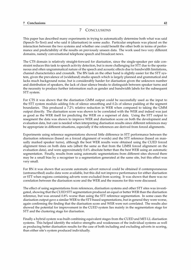
7 Conclusions 42

7 CONCLUSIONS

This paper has described many experiments in trying to automatically determine both what was said(Speech-To-Text) and who said it (diarisation) in some audio. Particular emphasis was placed on theinteraction between the two systems and whether one could benefit the other both in terms of perfor-mance and predictability of the results on previously unseen data. The work used two very differentdomains, namely conversational telephone speech and broadcast news.

The CTS domain is relatively straight-forward for diarisation, since the single-speaker per side con-straint reduces this task to speech activity detection, but is more challenging for STT due to the sponta-neous and often ungrammatical nature of the speech and acoustic effects due to bandwidth limitations,channel characteristics and crosstalk. The BN task on the other hand is slightly easier for the STT sys-tem, given the prevalence of (wideband) studio speech which is largely planned and grammatical andlacks much background noise, but is considerably harder for diarisation given the unknown numberand distribution of speakers, the lack of clear silence breaks to distinguish between speaker turns andthe necessity to produce further information such as gender and bandwidth labels for the subsequentSTT system.

For CTS it was shown that the diarisation GMM output could be successfully used as the input tothe STT system modulo adding 0.6s of silence smoothing and 0.2s of silence padding at the segmentboundaries. This produced a 7.2% relative reduction in WER when compared to taking the GMMoutput directly. The diarisation score was shown to be correlated with the WER and indeed was justas good as the WER itself for predicting the WER on a superset of data. Using the STT output toresegment the data was shown to improve WER and diarisation score on both the development andevaluation data, but care is needed when interpreting diarisation results since different references maybe appropriate in different situations, especially if the references are derived from forced alignments.

Experiments using reference segmentations showed little difference in STT performance between thediarisation references (based on a forced alignment of words) and the STT reference (based on man-ually marked speaker turns), although the best WER results were obtained using the CUED forcedalignment times on both data sets (albeit the same as that from the LIMSI forced alignment on theevaluation data), and were approximately 0.6% absolute better than the best WER using an automaticsegmentation. Finally, results from using automatic segmentations from different sites showed theremay be a small bias by a recogniser to a segmentation generated at the same site, but this effect wasvery small.

For BN it was shown that accurate automatic advert removal could be obtained if contemporaneous(untranscribed) audio data were available, but this did not improve performance for either diarisationor STT when regions containing adverts were excluded from scoring. It was shown that there was nocorrelation between the diarisation score and the WER and the reasons for this were discussed.

The effect of using segmentations from references, diarisation systems and other STT sites was investi-gated, showing that the CUED STT segmentation produced an equal or better WER than the diarisationreference, but was around 0.8% worse than using the STT reference segmentation. In some cases thediarisation output gave a similar WER to the STT-based segmentations, but in general they were worse,again confirming the finding that the diarisation score and WER were not correlated. The results alsoshowed the potential for improvement in the CUED system lies mainly in the segmentation stage forSTT and the clustering stage for diarisation.

Finally a hybrid system was built combining equivalent stages from the CUED and MIT-LL diarisationsystems. This helped identify the relative strengths and weaknesses of the individual systems as wellas producing better diarisation results for the case of both including and excluding adverts in scoring,than either site’s system produced individually.

8 Acknowledgements 43

8 ACKNOWLEDGEMENTS

The authors would like to thank Lori Lamel for providing LIMSI’s forced alignments for the dryrun andeval03 data; Daben Liu, Andreas Stolcke and George Saon for providing the STT segmentation(s) pro-duced by BBN, SRI and IBM respectively with their RT-03s CTS English evaluation systems; Jean-LucGauvain and Bing Xiang for providing the STT segmentation produced by LIMSI and BBN respectivelyfor the RT-03s BN English STT evaluation; and Daben Liu, Andreas Stolcke and Jean-Luc Gauvain fordiscussion of segmentation experiments performed at BBN, SRI and LIMSI.

This work was supported by DARPA grant MDA972-02-1-0013. The paper does not necessarily reflectthe position or the policy of the US Government and no official endorsement should be inferred.

A DATA

A.1 Broadcast News DataRT-02 data = dryrun data 19981214 2100 2200 MNB NBW(bnrt02 = bndry03) 19981215 2000 2100 PRI TWD

19981216 1830 1900 NBC NNW19981217 0130 0200 CNN HDL19981218 1600 1700 VOA ENG19981219 1830 1900 ABC WNT

STT BN RT-03 dev data 20010117 2000 2100 PRI TWD(bndev03) 20010120 1830 1900 ABC WNT

20010122 2100 2200 MNB NBW20010125 1830 1900 NBC NNW20010128 1400 1430 CNN HDL20010131 2000 2100 VOA ENG

Diarisation BN RT-03s dev data 20001006 2100 2200 VOA ENG(bndidev03) 20001008 1830 1900 NBC NNW

20001016 2000 2100 PRI TWD20001018 1830 1900 ABC WNT20001215 2100 2200 MNB NBW20001219 1400 1430 CNN HDL

Diarisation BN RT-03s eval data 20010228 2100 2200 MNB NBW(bneval03s) 20010217 1000 1030 VOA ENG

20010220 2000 2100 PRI TWD

Diarisation BN RT-03f dev data 20010206 1830 1900 ABC WNT(bndev03f) 20010221 1830 1900 NBC NNW

20010225 0900 0930 CNN HDL

STT eval data Diarisation BN RT-03s eval data +(bneval03) Diarisation BN RT-03f dev data


A.2 CTS DataRT-03 dryrun data sw4386 sw4634 sw4705 sw4806 sw 30410(ctsdry03) sw 30849 sw 31388 sw 39999 sw 45255 sw 46387

sw 46715 sw 47620

RT-02 eval data ctsdry03 + sw4394 sw4398 sw4409 sw4477(ctseval02) sw4490 sw4528 sw4535 sw4536 sw4578

sw4627 sw4639 sw4653 sw4730 sw4755sw4851 sw4866 sw 30016 sw 30223 sw 30352sw 30751 sw 30801 sw 30861 sw 30969 sw 30986sw 31032 sw 31131 sw 31195 sw 31483 sw 31493sw 31572 sw 31585 sw 32163 sw 45063 sw 45147sw 45187 sw 45284 sw 45458 sw 45501 sw 45734sw 45939 sw 46098 sw 46312 sw 46516 sw 46667sw 47205 sw 47435 sw 47566 sw 47610

Diarisation CTS RT-03s fsh 60262 fsh 60354 fsh 60416 fsh 60463 fsh 60493eval data fsh 60549 fsh 60571 fsh 60593 fsh 60627 fsh 60648(ctseval03s) fsh 60650 fsh 60720 fsh 60732 fsh 60797 fsh 60862

fsh 60885 fsh 61039 fsh 61192 sw 45097 sw 45142sw 45355 sw 45454 sw 45586 sw 45654 sw 45713sw 45727 sw 45819 sw 46140 sw 46412 sw 46512sw 46615 sw 46677 sw 46789 sw 46868 sw 47346sw 47411

Diarisation CTS RT-03f fsh 60386 fsh 60398 fsh 60441 fsh 60477 fsh 60568dev data fsh 60613 fsh 60668 fsh 60682 fsh 60784 fsh 60817(ctsdev03f) fsh 60818 fsh 60844 fsh 60874 fsh 61113 fsh 61130

fsh 61148 fsh 61225 fsh 61228 sw 45104 sw 45237sw 45481 sw 45626 sw 45837 sw 45856 sw 45973sw 46028 sw 46168 sw 46455 sw 46565 sw 46671sw 46732 sw 46938 sw 47038 sw 47073 sw 47175sw 47282

STT eval data Diarisation CTS RT-03s eval data +(ctseval03) Diarisation CTS RT-03f dev data

B ACCURACY OF CTS FORCED ALIGNMENTS

It was shown in section 4.5 that the diarisation scores were very sensitive to the way the diarisationreference file was generated. In particular, the accuracy of the reference word-times can make a largedifference to the scores and thus the reliability of the results. For the ctsdry03 development data, theword times George Doddington manually generated were used to define the reference, but since it isinfeasible to produce word-times manually for large data sets, the ctseval03 references were derivedfrom word times generated by an automatic forced alignment of the reference words to the audio.

The official RT-03s diarisation evaluation reference used times based on a forced alignment from theLDC. In addition to this, forced alignments were generated by both CUED and LIMSI on both thectseval03 and ctsdry03 data sets. In order to gauge the relative accuracy of the alignments, they werecompared to each other on both data sets, and to the manually-generated times on the ctsdry03 dataset.The results are given in Table 29.


ctseval03 data, 71528 wordsReference Hypothesis % Overlap Absolute Start Diff.(s) Absolute End Diff.(s)

Time/Words Mean SD Max Mean SD MaxLDC-FA LIMSI-FA 73.70/88.21 0.087 0.171 4.060 0.095 0.173 4.320LDC-FA CUED-FA 73.24/87.91 0.088 0.169 3.730 0.096 0.172 3.580LIMSI-FA CUED-FA 91.11/98.92 0.023 0.056 4.080 0.025 0.059 4.310

ctsdry03 data, 12188 wordsReference Hypothesis % Overlap Absolute Start Diff.(s) Absolute End Diff.(s)

Time/Words Mean SD Max Mean SD MaxManual LDC-FA 85.65/94.95 0.039 0.080 1.324 0.039 0.083 1.378Manual LIMSI-FA 88.34/99.43 0.026 0.042 1.200 0.031 0.053 1.367Manual CUED-FA 87.91/99.15 0.032 0.055 1.685 0.029 0.055 1.661LDC-FA LIMSI-FA 83.08/95.39 0.044 0.083 1.397 0.051 0.090 1.794LDC-FA CUED-FA 82.41/95.15 0.048 0.090 1.637 0.051 0.093 1.710LIMSI-FA CUED-FA 90.27/99.27 0.024 0.058 1.530 0.028 0.064 1.510

Table 29: Comparison of methods of generating word times on the ctsdry03 and ctseval03 data. Thepercentage of time that the corresponding words overlap for, and the percentage of correspondingwords that have some time overlap are given along with the mean, standard deviation and maximumabsolute difference between the corresponding times for both word starts and word ends.

The results on the larger ctseval03 data set show a high correlation between the CUED and LIMSIforced alignments, with the percentage of words that overlap in time rising from 88% when comparedto the LDC’s forced alignment to 99% when compared to each other. Similarly the mean and standarddeviation of both start and end time errors is considerably smaller when comparing the LIMSI/CUEDpair. This suggests that these times are more reliable.These findings are also backed up on the smallerctsdry03 data set. In this case, the LIMSI and CUED forced alignments have 99% of words overlappingwith the corresponding words in the manually generated times, as compared to 95% for the LDC. Themean and standard deviation of both start and end times errors when compared to the manual timesis also lower for both the CUED and LIMSI forced alignments, and again when comparing just theautomated systems the CUED and LIMSI alignments are the most correlated. For these reasons theRT-03f metadata evaluation, where word-level times are critical, will use the LIMSI forced alignmentsto generate the reference.

However, since we generated the CTS diarisation reference using 0.6s silence smoothing, the individualword times are generally less important apart from at the segment-level boundaries. The results of theword-level comparisons when only considering the first and last words in each segment on the ctsdry03data are given in Table 30. These show that the LDC-forced alignment gives more accurate times for thestart of the first word and end of the last word in each segment, consistent with the lower diarisationscore obtained for this case. This suggests that despite the poorer overall accuracy of word-times, theLDC forced alignment may be the most accurate for generating the diarisation reference.41

First word in segment only (N=1122) Last word in segment only (N=1122)Hypothesis % Overlap Absolute Start Diff.(s) %Overlap Absolute End Diff.(s)

Time/Words Mean SD Max Time/Words Mean SD MaxLDC-FA 91.66/98.13 0.015 0.069 1.071 93.43/99.73 0.023 0.087 1.378LIMSI-FA 83.01/99.38 0.048 0.078 1.200 85.84/99.55 0.077 0.106 1.367CUED-FA 81.79/98.66 0.064 0.076 1.273 87.45/99.11 0.059 0.089 1.258Table 30: Comparison of first and last words only to the manual times on the ctsdry03 data

41The CUED and LIMSI forced alignments were generated using the segment times from the STM file. These normally havesome silence padding added to them before distribution. At time of writing it is not clear if more accurate segment times wereuse to constrain the LDC forced alignments. This might explain why the first and last times in a segment are more accuratelypinpointed using the LDC forced alignment despite the poorer word-level times overall.

References 46

REFERENCES

Ajmera, J., Wooters, C., Peskin, B. and Oei, C. (2003). Speaker Segmentation and Clustering, Proc. Spring 2003 RichTranscription Workshop (RT-03s), Boston, MA.

Bimbot, F. and Mathan, L. (1993). Text-Free Speaker Recognition using an Arithmetic Harmonic Sphericity Mea-sure, Proc. European Conference on Speech Communication and Technology (Eurospeech), Vol. 1, pp. 169–172.

Chen, S. S. and Gopalakrishnam, P. S. (1998). Speaker, Environment and Channel Change Detection and Clusteringvia the Bayesian Information Criterion, Proc. 1998 DARPA Broadcast News Transcription and UnderstandingWorkshop, Lansdowne, VA, pp. 127–132.

Evermann, G. and Woodland, P. C. (2003). Design of Fast LVCSR Systems, Proc. Automatic Speech Recognition andUnderstanding Workshop (ASRU), St. Thomas, U.S. Virgin Islands, p. To appear.

Fiscus, J. G. (1997). A Post-Processing System To Yield Reduced Word Error Rates: Recognizer Output VotingError Reduction (ROVER), IEEE Workshop on Automatic Speech Recognition and Understanding.

Franco, H., Gadde, R., Graciarena, M., Stolcke, A., Vergyri, D., Wang, W. and Zheng, J. (2003). SRI CTS SystemImprovements, EARS STT Workshop.

Garofolo, J. S., Auzanne, C. G. P. and Voorhees, E. M. (2000). The TREC Spoken Document Retrieval Track: ASuccess Story, RIAO, Content-Based Multimedia Information Access, Vol. 1, Paris, France, pp. 1–20.

Garofolo, J. S., Lard, J. and Voorhees, E. M. (2001). 2000 TREC-9 Spoken Document Retrieval Track, The Ninth TextREtrieval Conference (TREC-9), http://trec.nist.gov/pubs/trec9/ .

Gauvain, J.-L. (2003). personal communication.Gauvain, J. L. and Barras, C. (2003). Speaker Diarization, Proc. Spring 2003 Rich Transcription Workshop (RT-03s),

Boston, MA.Gauvain, J. L., Lamel, L., Adda, G., Chen, L. and Schwenk, H. (2003). The LIMSI RT03 BN Systems, Proc. Spring

2003 Rich Transcription Workshop (RT-03s), Boston, MA.Hain, T. (2002). Implicit Pronunciation Modelling in ASR, Proc. ISCA ITRW Pronunciation Modeling and Lexicon

Adaptation (PMLA).Hain, T., Johnson, S. E., Tuerk, A., Woodland, P. C. and Young, S. J. (1998). Segment Generation and Cluster-

ing in the HTK Broadcast News Transcription System, Proc. 1998 DARPA Broadcast News Transcription andUnderstanding Workshop, Lansdowne, VA, pp. 133–137.

Hain, T., Woodland, P. C., Niesler, T. R. and Whittaker, E. W. D. (1999). The 1998 HTK System for Transcriptionof Conversational Telephone Speech, Proc. International Conference on Acoustics, Speech and Signal Processing(ICASSP), Phoenix, AZ.

Iyer, R., Kimball, O. and Matsoukas, S. (2003). Speech-to-Text Research at BBN : An Experiment in InexpensiveTranscription, EARS Mid-Year Meeting, Berkeley, CA.

Johnson, S. E. (1999). Who Spoke When? - Automatic Segmentation and Clustering for Determining SpeakerTurns, Proc. European Conference on Speech Communication and Technology (Eurospeech), pp. 2211–2214.

Johnson, S. E. and Woodland, P. C. (1998). Speaker Clustering Using Direct Maximisation of the MLLR-AdaptedLikelihood, Proc. International Conference in Spoken Language Processing (ICSLP), pp. 1775–1779.

Johnson, S. E. and Woodland, P. C. (2000). A Method for Direct Audio Search with Applications to Indexing andRetrieval, Proc. International Conference on Acoustics, Speech and Signal Processing (ICASSP), Vol. 3, Istanbul,Turkey, pp. 1427–1430.

Johnson, S. E., Jourlin, P., Sparck Jones, K. and Woodland, P. C. (2000). Spoken Document Retrieval for TREC-8 at Cambridge University, in E. M. Voorhees and D. K. Harman (eds), The Eighth Text REtrieval Conference(TREC-8), number SP 500-246, Department of Commerce, National Institute of Standards and Technology,Gaithersburg, MD, pp. 197–206.

Johnson, S. E., Jourlin, P., Sparck Jones, K. and Woodland, P. C. (2001). Spoken Document Retrieval for TREC-9 at Cambridge University, in E. M. Voorhees and D. K. Harman (eds), The Ninth Text REtrieval Conference(TREC-9), number SP 500-249, Department of Commerce, National Institute of Standards and Technology,Gaithersburg, MD, pp. 117–126.

Kim, D. Y., Evermann, G., Hain, T., Mrva, D., Tranter, S. E., Wang, L. and Woodland, P. C. (2003a). 2003 CU-HTKBroadcast News English System Development, Proc. Spring 2003 Rich Transcription Workshop (RT-03s), Boston,MA.

http://trec.nist.gov/pubs/trec9/

References 47

Kim, D. Y., Evermann, G., Hain, T., Mrva, D., Tranter, S. E., Wang, L. and Woodland, P. C. (2003b). Recent Advancesin Broadcast News Transcription, Proc. Automatic Speech Recognition and Understanding Workshop (ASRU), St.Thomas, U.S. Virgin Islands, p. To appear.

Liu, D. (2003). personal communication.Liu, D. and Kubala, F. (2003a). A Cross-Channel Modeling Approach for Automatic Segmentation of Conversa-

tional Telephone Speech, Proc. Automatic Speech Recognition and Understanding Workshop (ASRU), St. Thomas,U.S. Virgin Islands, p. To appear.

Liu, D. and Kubala, F. (2003b). Segmentation for Conversational Telephone Speech, Proc. Spring 2003 Rich Tran-scription Workshop (RT-03s), Boston, MA.

Matsoukas, S., Colthurst, T., Kimball, O., Solomonoff, A. and Gish, H. (2002). The 2002 BBN Byblos English LVCSRSystem, Proc. 2002 Rich Transcription Workshop (RT-02), Vienna, VA.

Matsoukas, S., Iyer, R., Kimball, O., Ma, J., Colthurst, T., Prasad, R. and Kao, C.-L. (2003). BBN CTS English System,Proc. Spring 2003 Rich Transcription Workshop (RT-03s), Boston, MA.

Moraru, D., Besacier, L., Meignier, S., Fredouille, C. and Bonastre, J.-F. (2003). ELISA, CLIPS and LIA NIST 2003segmentation, Proc. Spring 2003 Rich Transcription Workshop (RT-03s), Boston, MA.

Moraru, D., Meignier, S., Besacier, L., Bonastre, J.-F. and Magrin-Chagnolleau, I. (2003). The ELISA ConsortiumApproaches in Speaker Segmentation during the NIST 2002 Speaker Recognition Evaluation, Proc. Interna-tional Conference on Acoustics, Speech and Signal Processing (ICASSP), Vol. 2, Hong Kong, pp. 89–92.

Nguyen, L., Duta, N., Makhoul, J., Matsoukas, S., Schwartz, R., Xiang, B. and Xu, D. (2003). The BBN RT03 BNEnglish System, Proc. Spring 2003 Rich Transcription Workshop (RT-03s), Boston, MA.

Nguyen, P. and Junqua, J. C. (2003). PSTL’s Speaker Diarization, Proc. Spring 2003 Rich Transcription Workshop(RT-03s), Boston, MA.

NIST (2003a). Reference Cookbook for ”Who Spoke When” Diarization Task, v2.4,http://www.nist.gov/speech/tests/rt/rt2003/spring/docs/ref-cookbook-v2 4.pdf, 17th March 2003.

NIST (2003b). The Rich Transcription Fall 2003 (RT-03F) Evaluation Plan,http://www.nist.gov/speech/tests/rt/rt2003/fall/docs/rt03-fall-eval-plan-v9.pdf, 9th October 2003.

NIST (2003c). The Rich Transcription Spring 2003 (RT-03S) Evaluation Plan, version 4,http://www.nist.gov/speech/tests/rt/rt2003/spring/docs/rt03-spring-eval-plan-v4.pdf, 25th Feb 2003.

Povey, D. and Woodland, P. C. (2002). Minimum Phone Error And I-Smoothing For Improved DiscriminativeTraining, Proc. International Conference on Acoustics, Speech and Signal Processing (ICASSP).

Povey, D., Woodland, P. C. and Gales, M. J. F. (2003). Discriminative MAP for Acoustic Model Adaptation, Proc.International Conference on Acoustics, Speech and Signal Processing (ICASSP).

Reynolds, D. A., Torres, P. and Roy, R. (2003). EARS RT03s Diarization, Proc. Spring 2003 Rich Transcription Workshop(RT-03s), Boston, MA.

Reynolds, D., Quatieri, T. and Dunn, R. (2000). Speaker Verification Using Adapted Mixture Models, Digital SignalProcessing 10: 181–202.

Roy, R. R. (2003). Speech Metadata in Broadcast News, Thesis for Master of Engineering in Electrical Engineering andComputer Science, Massachusetts Institute of Technology, 21st May 2003.

Sanders, G. (2003). Who Spoke When - Speaker-ID and Speaker-Type Metadata Diarization., Proc. Spring 2003 RichTranscription Workshop (RT-03s), Boston, MA.

Saon, G., Zweig, G., Kingsbury, B. and Mangu, L. (2003). The IBM 2003 1xRT speech-to-text system, Proc. Spring2003 Rich Transcription Workshop (RT-03s), Boston, MA.

Stolcke, A., France, H., Gadde, R., Graciarena, M., Precoda, K., Venkataraman, A., Vergyri, D., Wang, W., Zheng,J., Huang, Y., Peskin, B., Bulyko, I., Ostendorf, M. and Kirchhoff, K. (2003). Speech-to-Text research at SRI-ICSI-UW, Proc. Spring 2003 Rich Transcription Workshop (RT-03s), Boston, MA.

Tranter, S. E., Yu, K. and the HTK STT team (2003). Diarisation for RT-03s at Cambridge University., Proc. Spring2003 Rich Transcription Workshop (RT-03s), Boston, MA.

Wilcox, L., Chen, F., Kimber, D. and Balasubramanian, V. (1994). Segmentation of Speech Using Speaker Iden-tification, Proc. International Conference on Acoustics, Speech and Signal Processing (ICASSP), Vol. 1, Adelaide,Australia, pp. 161–164.

Woodland, P. C. (2002). The Development of the HTK Broadcast News Transcription System: An Overview, SpeechCommunication 37: 291–299.

References 48

Woodland, P. C., Chan, H. Y., Evermann, G., Gales, M. J. F., Hain, T., Kim, D. Y., Liu, X., Mrva, D., Povey, D., Tranter,S. E., Wang, L. and Yu, K. (2003). 2003 CU-HTK English CTS System, Proc. Spring 2003 Rich TranscriptionWorkshop (RT-03s), Boston, MA.

Woodland, P. C., Evermann, G., Gales, M. J. F., Hain, T., Liu, X., Moore, G. L., Povey, D. and Wang, L. (2002).CU-HTK April 2002 Switchboard System, Proc. 2002 Rich Transcription Workshop (RT-02), Vienna, VA.

Woodland, P. C., Hain, T., Moore, G. L., Niesler, T. R., Povey, D., Tuerk, A. and Whittaker, E. W. D. (1999). The 1998HTK Broadcast News Transcription System: Development and Results, Proc. 1999 DARPA Broadcast NewsWorkshop, Herndon, VA, pp. 265–270.

Zhan, P., Wegmann, S. and Gillick, L. (1999). Dragon Systems’ 1998 Broadcast News Transcription System ForMandarin, Proc. 1999 DARPA Broadcast News Workshop, Herndon, VA, pp. 183–186.

Note many of the Cambridge University publications are available fromhttp://mi.eng.cam.ac.uk/reportsand see also the CUED EARS-project reference pagehttp://mi.eng.cam.ac.uk/research/projects/EARS/references.html

Publications from the Rich Transcription Workshops can be found throughhttp://www.nist.gov/speech/publications

http://mi.eng.cam.ac.uk/reports

http://mi.eng.cam.ac.uk/research/projects/EARS/references.html

http://www.nist.gov/speech/publications

An Investigation into the Interactions between Speaker...

Documents

Transcript of An Investigation into the Interactions between Speaker...