An Introduction to the Finite Element Method (FEM) for Differential ...

An Introduction to theFinite Element Method (FEM)for Differential Equations in 1D
Mohammad Asadzadeh
June 24, 2015


Contents
1 Introduction 1
1.1 Ordinary differential equations (ODE) . . . . . . . . . . . . . 1
1.2 Partial differential equations (PDE) . . . . . . . . . . . . . . . 2
1.2.1 Exercises . . . . . . . . . . . . . . . . . . . . . . . . . . 8
2 Polynomial Approximation in 1d 9
2.1 Overture . . . . . . . . . . . . . . . . . . . . . . . . . . . . . . 9
2.1.1 Basis function in nonuniform partition . . . . . . . . . 14
2.2 Variational formulation for (IVP) . . . . . . . . . . . . . . . . 17
2.3 Galerkin finite element method for (2.1.1) . . . . . . . . . . . 19
2.4 A Galerkin method for (BVP) . . . . . . . . . . . . . . . . . . 21
2.4.1 The nonuniform version . . . . . . . . . . . . . . . . . 26
2.5 Exercises . . . . . . . . . . . . . . . . . . . . . . . . . . . . . . 27
3 Interpolation, Numerical Integration in 1d 31
3.1 Preliminaries . . . . . . . . . . . . . . . . . . . . . . . . . . . 31
3.2 Lagrange interpolation . . . . . . . . . . . . . . . . . . . . . . 39
3.3 Numerical integration, Quadrature rules . . . . . . . . . . . . 41
3.3.1 Composite rules for uniform partitions . . . . . . . . . 44
3.3.2 Gauss quadrature rule . . . . . . . . . . . . . . . . . . 48
4 Two-point boundary value problems 53
4.1 A Dirichlet problem . . . . . . . . . . . . . . . . . . . . . . . 53
4.2 The finite element method (FEM) . . . . . . . . . . . . . . . . 58
4.3 Error estimates in the energy norm . . . . . . . . . . . . . . . 59
4.4 FEM for convection–diffusion–absorption BVPs . . . . . . . . 65
4.5 Exercises . . . . . . . . . . . . . . . . . . . . . . . . . . . . . . 72
iii

iv CONTENTS
5 Scalar Initial Value Problems 815.1 Solution formula and stability . . . . . . . . . . . . . . . . . . 825.2 Finite difference methods . . . . . . . . . . . . . . . . . . . . . 835.3 Galerkin finite element methods for IVP . . . . . . . . . . . . 86
5.3.1 The continuous Galerkin method . . . . . . . . . . . . 875.3.2 The discontinuous Galerkin method . . . . . . . . . . . 90
5.4 Exercises . . . . . . . . . . . . . . . . . . . . . . . . . . . . . . 92
6 Initial Boundary Value Problems in 1d 956.1 Heat equation in 1d . . . . . . . . . . . . . . . . . . . . . . . . 95
6.1.1 Stability estimates . . . . . . . . . . . . . . . . . . . . 966.1.2 FEM for the heat equation . . . . . . . . . . . . . . . . 1006.1.3 Exercises . . . . . . . . . . . . . . . . . . . . . . . . . . 104
6.2 The wave equation in 1d . . . . . . . . . . . . . . . . . . . . . 1066.2.1 Wave equation as a system of PDEs . . . . . . . . . . 1076.2.2 The finite element discretization procedure . . . . . . 1086.2.3 Exercises . . . . . . . . . . . . . . . . . . . . . . . . . . 111
A Answers to Exercises 115
B Algorithms and MATLAB Codes 121
Table of Symbols and Indices 135

CONTENTS v
Preface and acknowledgments. This text is an elementary approach tofinite element method used in numerical solution of differential equations inone space dimension. The purpose is to introduce students to piecewise poly-nomial approximation of solutions using a minimum amount of theory. Thepresented material in this note should be accessible to students with knowl-edge of calculus of single- and several-variables and linear algebra. The theoryis combined with approximation techniques that are easily implemented byMatlab codes presented at the end.
During several years, many colleagues have been involved in the design,presentation and correction of these notes. I wish to thank Niklas Erikssonand Bengt Svensson who have read the entire material and made many valu-able suggestions. Niklas has contributed to a better presentation of the textas well as to simplifications and corrections of many key estimates that hassubstantially improved the quality of this lecture notes. Bengt has made allxfig figures. The final version is further polished by John Bondestam Malm-berg and Tobias Geback who, in particular, have many useful input in theMatlab codes.

vi CONTENTS
void
Chapter 1
Introduction
In this lecture notes we present an introduction to approximate solutions fordifferential equations. A differential equation is a relation between a functionand its derivatives. In case the derivatives that appear in a differential equa-tion are only with respect to one variable, the differential equation is calledordinary. Otherwise it is called a partial differential equation. For example,
du
dt− u(t) = 0, (1.0.1)
is an ordinary differetial equation, whereas
∂u
∂t− ∂2u
∂x2= 0, (1.0.2)
is a partial differential (PDE) equation. In (1.0.2) ∂u∂t, ∂2u
∂x2 denote the partialderivatives. Here t denotes the time variable and x is the space variable. Weshall only study one space dimentional equations that are either stationary(time-independent) or time dependent. Our focus will be on the followingequations:
1.1 Ordinary differential equations (ODE)
• An example of population dynamic as in (1.0.1)
du
dt− λu(t) = f(t), (1.1.1)
1
2 CHAPTER 1. INTRODUCTION
where λ is a constant and f is a source function.• A stationary (time-independent) heat equation as
−d2u
dx2= f(x), (1.1.2)
• A stationary convection-diffusion equation
−d2u
dx2+du
dx= f(x), (1.1.3)
where f(x) is a source function.
1.2 Partial differential equations (PDE)
• The heat equation∂u
∂t− ∂2u
∂x2= f(x). (1.2.1)
• The wave equation∂2u
∂t2− ∂2u
∂x2= f(x). (1.2.2)
• The time depending convection-diffusion or reaction-diffusion equation
∂u
∂t− ∂2u
∂x2+∂u
∂x= f(x). (1.2.3)
Some notation. For convenince we shall use the following notation:
u =∂u
∂t, u =
∂2u
∂t2, u′ =
∂u
∂x, u′′ =
∂2u
∂x2.
Example 1.1 (Initial Conditions). Consider the simple equation u(t) = t.Evidently, u(t) = t2/2, is a solution. But, for any constant C, t2/2 + C isalso a solution. In this way we have infintely many solutions (one for eachconstant C). To determine a unique solution we need to supply the equationwith one extra condition. Since the time variable t is always assumed to bet ≥ 0, if we know the value of u(t), e.g., at the beginning, i.e., the initialvalue e.g., u(0) = 3, then u(t) = t2/2+ 3 is the unique solution to the initialvalue problem: u(t) = t, u(0) = 3. A differential equation associated withinitial conditions is an initial value problem.

1.2. PARTIAL DIFFERENTIAL EQUATIONS (PDE) 3
Example 1.2 (Boundary Conditions). Likewise u(x) = −x2/2 is a solu-tion to −u′′(x) = 1. But also all u(x) = −x2/2 + Ax + B are solutions, forall arbitrary constants A and B. Therefore, to determine a unique solutionu(x) we need to determine some fixed values for A and B, hence we needto supply two conditions. Here if e.g., x belongs to a bounded interval, say,[0, 1], then given the boundary values u(0) = 1 and u(1) = 0, we get fromu(x) = −x2/2 + Ax + B that B = 1 and A = −1/2. Thus the solution tothe the initial boundary value problem: −u′′(x) = 1, u(0) = 1, u(1) = 0is: u(x) = −x2/2 − x/2 + 1. The generale rule is that one should supply asmany conditions as the highest ordre of the derivative in each variable. So,for example, for the hear equation u − u′′ = 0, to get a unique solution wenedd to supply one initial condition (there is one time derivative in the equa-tion) and two boundary conditions (there are two derivatives in x), whereasfor the wave equation u − u′′ = 0 we have to give two conditions in eachvariable x and t. A differential equation with supplied boundary conditionsis a boundary value problem.
Objectives: For f being a simple elementary function (a polynomial, atrigonometric, or exponential type function or a combination of them), theequations (1.1.1)-(1.2.3), associated with suitable initial and boundary condi-tions, have often closed form analytic solutions. But real problems: generaltwo and three dimensional problems, modeled by equations with variablecefficients and in complex geometry, are seldom analytically solvable.
In this note our objective is to introduce numerical methods that ap-proximate solutions for differential equations by polynomials. To check thequality (reliability and efficiency) of these numerical methods, we choose toapply them to the equations (1.1.1)-(1.2.3), where we already know their an-alytic solutions. Below we shall give examples of analytic solutions to ODEs:(1.1.1)-(1.1.3). For examples on analytic solutions for the PDEs: (1.2.1)-(1.2.3), we refer to the separation of variables technique introduced in thesecond part of our course.
Example 1.3. Determine the solution to the initial value problem
u(t)− λu(t) = 0, u(0) = u0, (1.2.4)
assuming that u(t) > 0, for all t, λ = 1 and u0 = 2.
Solution. Since u(t) 6= 0, for all t, we may divide the equation (1.2.4) by
4 CHAPTER 1. INTRODUCTION
u(t) and get u(t)u(t)
= λ. Relabeling t by s and integrating over (0, t) we get
∫ t
0
u(s)
u(s)ds = λ
∫ t
0
ds =⇒[ln u(s)
]t0= λ[s]t0. (1.2.5)
Hence we have
ln u(t)− ln u(0) = λt or lnu(t)
u(0)= λt. (1.2.6)
Thusu(t)
u(0)= eλt, i.e. u(t) = u0e
λt. (1.2.7)
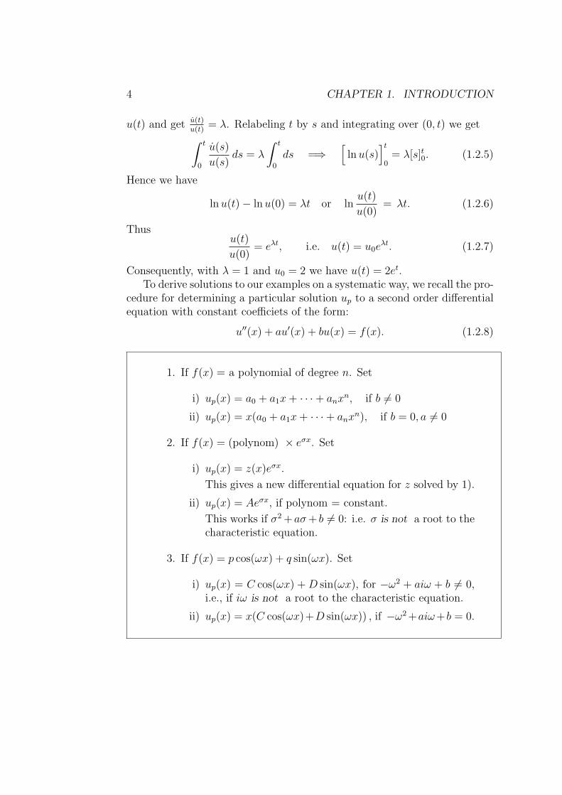
Consequently, with λ = 1 and u0 = 2 we have u(t) = 2et.To derive solutions to our examples on a systematic way, we recall the pro-
cedure for determining a particular solution up to a second order differentialequation with constant coefficiets of the form:
u′′(x) + au′(x) + bu(x) = f(x). (1.2.8)
1. If f(x) = a polynomial of degree n. Set
i) up(x) = a0 + a1x+ · · ·+ anxn, if b 6= 0
ii) up(x) = x(a0 + a1x+ · · ·+ anxn), if b = 0, a 6= 0
2. If f(x) = (polynom) × eσx. Set
i) up(x) = z(x)eσx.
This gives a new differential equation for z solved by 1).
ii) up(x) = Aeσx, if polynom = constant.
This works if σ2+ aσ+ b 6= 0: i.e. σ is not a root to thecharacteristic equation.
3. If f(x) = p cos(ωx) + q sin(ωx). Set
i) up(x) = C cos(ωx) +D sin(ωx), for −ω2 + aiω + b 6= 0,i.e., if iω is not a root to the characteristic equation.
ii) up(x) = x(C cos(ωx)+D sin(ωx)) , if −ω2+aiω+b = 0.

1.2. PARTIAL DIFFERENTIAL EQUATIONS (PDE) 5
Example 1.4. Find all solutions to the differential equation
u′′(x)− u(x) = cos(x). (1.2.9)
Solution. Due to the highest number of derivatives (here 2 which is alsocalled the order of this differential equation), we shall have solutions depend-ing on two arbitrary constants. As we mentioned earilear a unique solutionwould require supplying 2 conditions, which we skip in this problem.
We note that the characteristic equation to this differentisal equatios:r2 − 1 = 0 has the roots ω = ±1. We split the solution procedure in 3 steps:
Step 1: According to the table above we choose a particular solution up(x)of the form
up(x) = A cos x+ B sin x. (1.2.10)
Differentiating twice and inserting in the equation (1.2.9) yeilds
u′p(x) = −A sin x+ B cos x
u′′p(x) = −A cos x−B sin x
u′′p(x)− up(x) = −2A cos x− 2B sin x = cos x
identifying the coefficients yields A = −12, B = 0. Thus
up(x) = −1
2cosx (1.2.11)
Step 2: The homogeneous solution is given by the standard ansatz
uh(x) = C1er1x + C2e
r2x, (1.2.12)
where C1 and C2 are arbitrary constants and r1 = 1 and r2 = −1 are theroots of the characteristic equation. Hence
uh(x) = C1ex + C2e
−x. (1.2.13)
Step 3: Finally, the general solution is given by adding the particular andhomogeneous solutions
u(x) = −1
2cos x+ C1e
x + C2e−x. (1.2.14)
In the above example we obtained general solutions depending on two con-stants. Below we shall demonstrate an example where, supplying two bound-ary conditions, we obtain a unique solution
6 CHAPTER 1. INTRODUCTION
Example 1.5. Determine the unique solution of the following boundary valueproblem
u′′ + 2u′ + u = 1 + x+ 2 sin x, u(0) = 1, u′(0) = 0. (1.2.15)
Homogeneous solution:The characteristic equation for the differential equation (1.2.15) is given by
r2 + 2r + 1 = 0, and has dubbel root r1,2 = −1. (1.2.16)
This gives the homogeneous solutions as
uh = (C1 + C2x)e−x. (1.2.17)
Particular solution:The particula solution can be written as sum of two particular solution tothe following equations:
u′′1 + 2u′1 + u1 = 1 + x, (1.2.18)
andu′′2 + 2u′2 + u2 = 2 sin x. (1.2.19)
Since the differential equation is linear, a concept justified by the relation
(au1 + bu2)′ = au′1 + bu′2 and ∀a, b ∈ R,
thus u = u1 + u2 will be a particular solution for (1.2.15). Using the table ofparticular solutions, we may insert u1(x) = Ax + B, as particular solution,in (1.2.18) and get
2A+ Ax+ B = 1 + x. (1.2.20)
Identifying the coefficients in (1.2.20) gives A = 1 and B = −1. Hence
u1(x) = x− 1.
Once again using the table of particular solutions, we may insert u2(x) =A sin x+ B cosx, as particular solution, in (1.2.19) and get
2A cos x− 2B sin x = 2 sin x. (1.2.21)
Identifying the coefficients in (1.2.21) gives A = 0 and B = −1. Hence
u2(x) = − cos x.

1.2. PARTIAL DIFFERENTIAL EQUATIONS (PDE) 7
Thus the general solution is given by
u = uh + u1 + u2 = (C1 + C2x)e−x + (x− 1)− cosx. (1.2.22)
Now we use the boundary conditions and determine the coefficients C1 andC2. Observe that
u′ = C2e−x − (C1 + C2x)e
−x + 1 + sin x,
and we have that
u(0) = 1 =⇒ C1 − 1− 1 = 1 =⇒ C1 = 3.
Further
u′(0) = 0 =⇒ C2 − C1 + 1 = 0 =⇒ C2 = C1 − 1 =⇒ C2 = 2.
Thus the final solution is
u(x) = x− 1− cos x+ e−x(3 + 2x).
Summary: These examples of ODEs can serve as a sort of warm up. As wementioned the corresponding analytical solutions for our PDEs is the subjectof Fourier analysis that we cover on the second part of this course. Theremaing chapters will be devoted to the approximation methods for solutionof our ODEs and PDEs. We shall approximate the solutions with, piecewise,polynomials. Such approximations are known as the Galerkin finite elementmethods (FEM). In its final step, a finite element procedure yields a linearsystem of equations (LSE) where the unknowns are the approximate values ofthe solution at certain points. Then, an approximate solution is constructedby adapting, piecewise, polynomials of certain degree to these point values.
The entries of the coefficient matrix and the right hand side of FEM’sfinal linear system of equations consist of integrals which are not alwayseasily computable. Therefore, numerical integration are introduced to ap-proximate such integrals. Interpolation techniques are introduced for bothaccurate polynomial approximations and to derive error estimates necessaryin determining qualitative properties of the approximate solutions. That isto show how the approximate solution approaches the exact solution as thenumber of unknowns increase.

8 CHAPTER 1. INTRODUCTION
1.2.1 Exercises
Problem 1.1. Find all solutions to the following homogeneous (their righthand side is zero “0”) differential equations
a) u′′ − 3u′ + 2u = 0 b) u′′ + 4u = 0 c) u′′ − 6u′ + 9u = 0
Problem 1.2. Find all solutions to the following non-homogeneous (theirright hande side are non-zero ” 6= 0′′) differential equations
a) u′′+2u′+2u = (1+x)2 b) u′′+u′+2u = sin x c) u′′+3u′+2u = ex
Problem 1.3. Find a particular solution to each of the following equationsa) u′′ − 2u′ = x2 b) u′′ + u = sin x c) u′′ + 3u′ + 2u = ex + sin x.
Problem 1.4. Solve the boundary value problem for all x ∈ (0, 1),
−u′′ + u = f(x), u(0) = u(1) = 0,
a) for f(x) = 0, b) for f(x) = x, c) for f(x) = sin(πx),
Problem 1.5. Solve the following boundary value problemsa) −u′′ = x− 1, 0 < x < π, u′(0) = u(π) = 0,b) −u′′ = x, 0 < x < π, u′(0) = u′(1) = 0.

Chapter 2
Polynomial Approximation in1d
Our objective is to present the finite element method (FEM) as an approximationtechnique for solution of differential equations using piecewise polynomials. Thischapter is devoted to some necessary mathematical environments and tools, aswell as a motivation for the unifying idea of using finite elements: A numericalstrategy arising from the need of changing a continuous problem into a discreteone. The continuous problem will have infinitely many unknowns (if one asks foru(x) at every x), and it cannot be solved exactly on a computer. Therefore ithas to be approximated by a discrete problem with a finite number of unknowns.The more unknowns we keep, the better the accuracy of the approximation willbe, but at a greater computational expense.
2.1 Overture
Below we shall introduce a few standard examples of classical differentialequations and some regularity requirements.
Ordinary differential equations (ODEs)An initial value problem (IVP), for instance a model in population dynamicswhere u(t) is the size of the population at time t, can be written as
u(t) = λu(t), 0 < t < T, u(0) = u0, (2.1.1)
where u(t) = dudt
and λ is a positive constant. For u0 > 0 this problem hasthe increasing analytic solution u(t) = u0e
λ·t, which blows up as t→ ∞.
9
10 CHAPTER 2. POLYNOMIAL APPROXIMATION IN 1D
• Numerical solutions of (IVP)
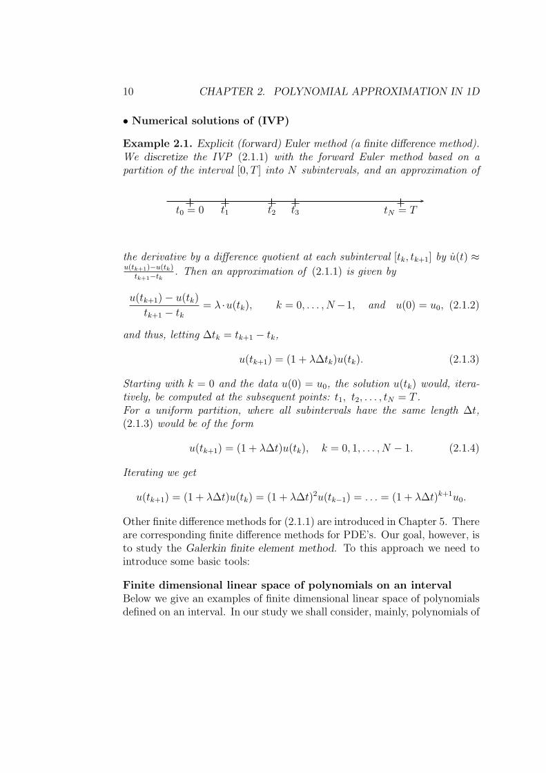
Example 2.1. Explicit (forward) Euler method (a finite difference method).We discretize the IVP (2.1.1) with the forward Euler method based on apartition of the interval [0, T ] into N subintervals, and an approximation of
t0 = 0 t1 t2 t3 tN = T
the derivative by a difference quotient at each subinterval [tk, tk+1] by u(t) ≈u(tk+1)−u(tk)
tk+1−tk. Then an approximation of (2.1.1) is given by
u(tk+1)− u(tk)
tk+1 − tk= λ ·u(tk), k = 0, . . . , N−1, and u(0) = u0, (2.1.2)
and thus, letting ∆tk = tk+1 − tk,
u(tk+1) = (1 + λ∆tk)u(tk). (2.1.3)
Starting with k = 0 and the data u(0) = u0, the solution u(tk) would, itera-tively, be computed at the subsequent points: t1, t2, . . . , tN = T .For a uniform partition, where all subintervals have the same length ∆t,(2.1.3) would be of the form
u(tk+1) = (1 + λ∆t)u(tk), k = 0, 1, . . . , N − 1. (2.1.4)
Iterating we get
u(tk+1) = (1 + λ∆t)u(tk) = (1 + λ∆t)2u(tk−1) = . . . = (1 + λ∆t)k+1u0.
Other finite difference methods for (2.1.1) are introduced in Chapter 5. Thereare corresponding finite difference methods for PDE’s. Our goal, however, isto study the Galerkin finite element method. To this approach we need tointroduce some basic tools:
Finite dimensional linear space of polynomials on an intervalBelow we give an examples of finite dimensional linear space of polynomialsdefined on an interval. In our study we shall consider, mainly, polynomials of

2.1. OVERTURE 11
degree 1. Higher degree polynomials are studied in some details in Chapter3: the polynomial interpolation in 1D.
We define P (q)(a, b) := Space of polynomials of degree ≤ q, a ≤ x ≤ b.A possible basis for P (q)(a, b) would be xjqj=0 = 1, x, x2, x3, . . . , xq. Theseare, in general, non-orthogonal polynomials and may be orthogonalized bythe Gram-Schmidt procedure. The dimension of Pq is therefore q + 1.
Example 2.2. For linear approximation we shall only need the basis func-tions 1 and x. An alternative linear basis function on the interval [a, b] isgiven by two functions λa(x) and λb(x) with the additional property
λa(x) =
1, x = a
0, x = band λb(x) =
1, x = b
0, x = 0.
Being linear λa(x) = Ax+B. To determine the coefficients A and B we havethat
λa(a) = 1 =⇒ Aa+ B = 1
λa(b) = 0 =⇒ Ab+ B = 0
Subtracting the two relations above we get A(b − a) = −1 =⇒ A = −1b−a
.
Then, from the second relation: B = −Ab we get B = bb−a
. Thus,
λa(x) =b− x
b− a. Likewise λb(x) =
x− a
b− a.
1
a bx
λa(x) λb(x)
Figure 2.1: Linear basis functions λa(x) and λb(x).
Note that
λa(x) + λb(x) = 1, and aλa(x) + bλb(x) = x.
12 CHAPTER 2. POLYNOMIAL APPROXIMATION IN 1D
Thus, we get the original basis functions: 1 and x for the linear polynomialfunctions, as a linear combination of the basis functions λa(x) and λb(x).Hence, any linear function f(x) on an interval [a, b] can be written as:
f(x) = f(a)λa(x) + f(b)λb(x). (2.1.5)
This is easily seen by the fact that the right hand side in (2.1.5) yields:
f(a)λa(a) + f(b)λb(a) = f(a)× 1 + f(b)× 0 = f(a),
f(a)λa(b) + f(b)λb(b) = f(a)× 0 + f(b)× 1 = f(b).
That is the two sides in (2.1.5) agree in two distinct points, therefore, beinglinear, they represent the same function.
Example 2.3. Let [a, b] = [0, 1] then λ0(x) = 1−x and λ1(x) = x. Considerthe linear function f(x) = 3x+ 5/2. Then f(0) = 5/2, f(1) = 11/2 and
f(0)λ0(x) + f(1)λ1(x) =5
2(1− x) +
11
2x = 3x+ 5/2 = f(x).
Definition 2.1. Let f(x) be a real valued function definied on R or on aninterval that contains [a, b]. A linear interpolant of f(x) on a and b is alinear function π1f(x) such that π1f(a) = f(a) and π1f(b) = f(b).
As in verification of (2.1.5), we have also π1f(x) = f(a)λa(x)+f(b)λb(x) :
π1f(x) = f(a)b− x
b− a+ f(b)
x− a
b− a.
Below, for simplicity, first we shall assume a uniform partition of the interval[0, 1] into M + 1 subintervals of the same size h, i.e., we let xj = jh, andconsider subintervals Ij := [xj−1, xj ] = [(j − 1)h, jh] for j = 1, . . . ,M + 1.Then setting a = xj−1 = (j − 1)h and b = xj = jh we may define
λj−1(x) = −x− jh
hand λj(x) =
x− (j − 1)h
h.
We denote the space of all continuous piecewise linear polynomial func-tions on Th, by Vh. Let
V 0h := v : v ∈ Vh, v(0) = v(1) = 0.
2.1. OVERTURE 13
a
π1f(x)
bx
y
f(x)
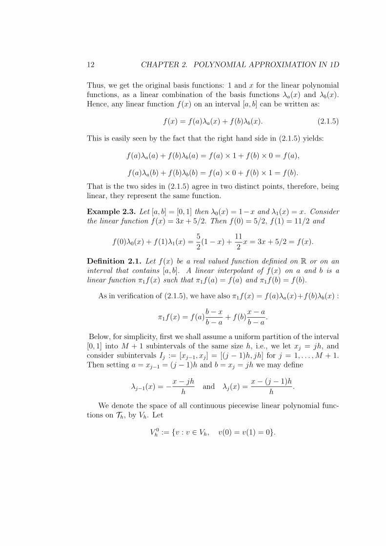
Figure 2.2: The linear interpolant π1f(x) on a single interval.
x0 x2x1x
y
xj−1 xj xM xM+1 = 1h h h
Figure 2.3: An example of a function in V 0h with uniform partition.
Applying (2.1.5), on each subinterval Ij, j = 1, . . . ,M +1, (using λj(x), j =1, . . . ,M) we can easily construct the functions belonging V 0
h . To construct afunction v(x) ∈ Vh we shall also need additional basis functions λ0(x) and/orλM+1(x) if v(0) 6= 0, and/or v(1) 6= 0, corresponding to non-vanishing datain the boundary value problems.
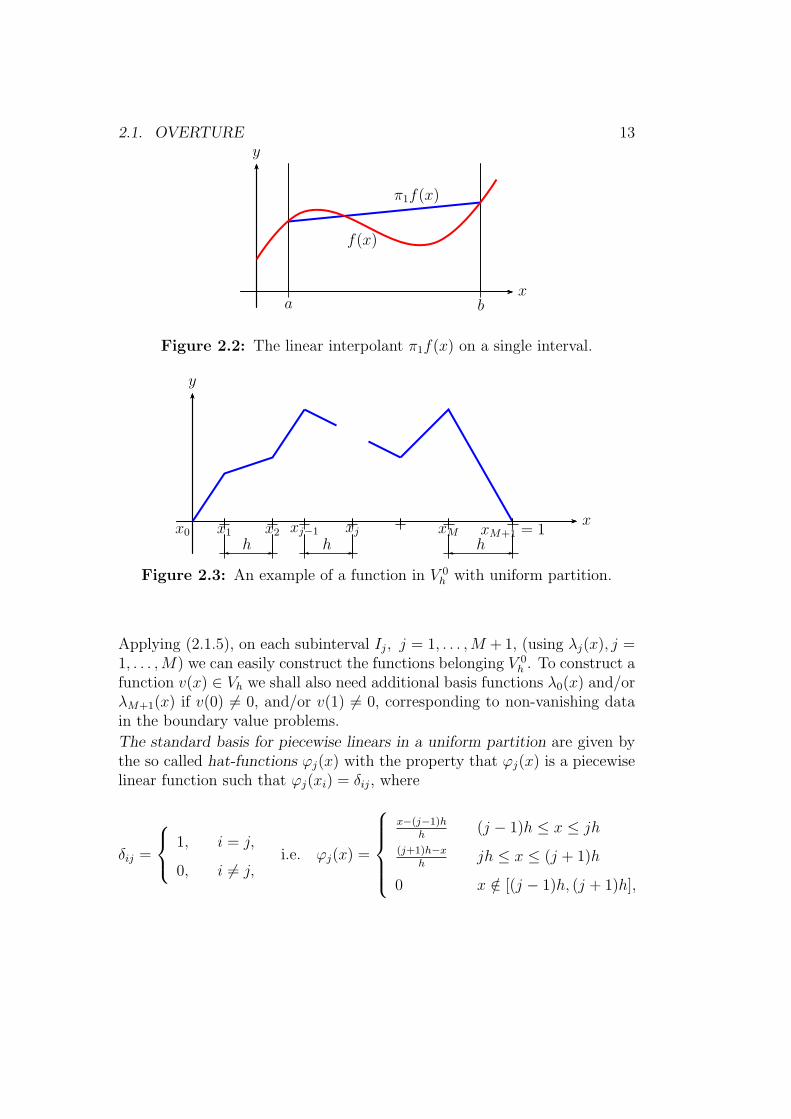
The standard basis for piecewise linears in a uniform partition are given bythe so called hat-functions ϕj(x) with the property that ϕj(x) is a piecewiselinear function such that ϕj(xi) = δij, where
δij =
1, i = j,
0, i 6= j,i.e. ϕj(x) =
x−(j−1)hh
(j − 1)h ≤ x ≤ jh
(j+1)h−xh
jh ≤ x ≤ (j + 1)h
0 x /∈ [(j − 1)h, (j + 1)h],
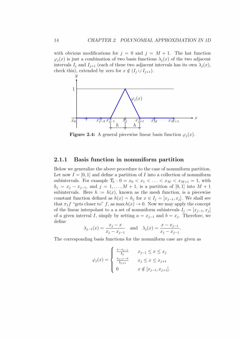
14 CHAPTER 2. POLYNOMIAL APPROXIMATION IN 1D
with obvious modifications for j = 0 and j = M + 1. The hat functionϕj(x) is just a combination of two basis functions λj(x) of the two adjacentintervals Ij and Ij+1 (each of these two adjacent intervals has its own λj(x),check this), extended by zero for x /∈ (Ij ∪ Ij+1).
x0 xj−2
1
x
y
xj−1 xj xj+1 xM xM+1
h h
ϕj(x)
Figure 2.4: A general piecewise linear basis function ϕj(x).
2.1.1 Basis function in nonuniform partition
Below we generalize the above procedure to the case of nonuniform partition.Let now I = [0, 1] and define a partition of I into a collection of nonuniformsubintervals. For example Th : 0 = x0 < x1 < . . . < xM < xM+1 = 1, withhj = xj − xj−1, and j = 1, . . . ,M + 1, is a partition of [0, 1] into M + 1subintervals. Here h := h(x), known as the mesh function, is a piecewiseconstant function defined as h(x) = hj for x ∈ Ij = [xj−1, xj]. We shall seethat π1f “gets closer to” f , as maxh(x) → 0. Now we may apply the conceptof the linear interpolant to a a set of nonuniform subintevals Ij := [xj−1, xj]of a given interval I, simply by setting a = xj−1 and b = xj. Therefore, wedefine
λj−1(x) =xj − x
xj − xj−1
and λj(x) =x− xj−1
xj − xj−1
.
The corresponding basis functions for the nonuniform case are given as
ϕj(x) =
x−xj−1
hjxj−1 ≤ x ≤ xj
xj+1−x
hj+1xj ≤ x ≤ xj+1
0 x /∈ [xj−1, xj+1].

2.1. OVERTURE 15
x0 x2x1x
y
xj−1 xj xM xM+1 = 1h2 hj hM+1
Figure 2.5: An example of a function in V 0h .
Again with obvious modifications for j = 0 and j =M + 1.
x0 xj−2
1
x
y
xj−1 xj xj+1 xM xM+1hj hj+1
ϕj(x)
Figure 2.6: A general piecewise linear basis function ϕj(x).
Vector spacesTo establish a framework we introduce some basic mathematical concepts:
Definition 2.2. A set V of functions or vectors is called a linear space, ora vector space, if for all u, v ∈ V and all α ∈ R (real number), we have that
(i) u+ v ∈ V, (closed under addition)
(ii) αu ∈ V, (closed under multiplication by scalars),
(iii) ∃ (−u) ∈ V : u+ (−u) = 0, (closed under inverse),
(2.1.6)
where (i) and (ii) obey the usual rules of addition and multiplication byscalars. Observe that α = 0 in (ii) (or (iii) and (i), with v = (−u)), impliesthat 0 (zero vector) is an element of every vector space.

16 CHAPTER 2. POLYNOMIAL APPROXIMATION IN 1D
Definition 2.3. A scalar product (inner product) is a real valued operatoron V ×V , viz 〈u, v〉 : V ×V → R such that for all u, v, w ∈ V and all α ∈ R,
(i) 〈u, v〉 = 〈v, u〉, (symmetry)
(ii) 〈u+ αv, w〉 = 〈u, w〉+ α〈v, w〉, (bi-linearity)
(iii) 〈v, v〉 ≥ 0, ∀v ∈ V, (positivity)
(iv) 〈v, v〉 = 0,⇐⇒ v = 0 (positive definiteness).
(2.1.7)
Definition 2.4. A vector space V is called an inner product space if V isassociated with a scalar product 〈·, ·〉, defined on V × V .
Example 2.4. A usual example of scalar product of two functions u and vdefined on an interval [a, b], known as the L2 scalar product, is defined by
〈u, v〉 :=∫ b
a
u(x)v(x)dx. (2.1.8)
Here are examples of some vector spaces that are also linear productspaces associated with the scalar product defined by (2.1.8).
•C(a, b): The space of continuous functions on an interval (a, b),•P (q)[a, b]: the space of all polynomials of degree ≤ q on C[a, b] and•Vh(a, d) and V 0
h (a, b) defined above.The reader may easily check that all the properties (i) − (iv), in the
definition, for the scalar product are fullfiled for these spaces.
Definition 2.5. Two (real-valued) functions u(x) and v(x) are called orthog-onal if 〈u, v〉 = 0. The orthogonality is also denoted by u ⊥ v.
Example 2.5. For the functions u(x) = 1 and v(x) = x, we have that∫ 1
−1
u(x)v(x)dx =
∫ 1
−1
1×x dx = 0,
∫ 1
0
u(x)v(x)dx =
∫ 1
0
1×x dx = 1/2 6= 0.
Thus, 1 and x are orthogonal on the interval [−1, 1], but not on [0, 1].
Definition 2.6 (Norm). If u ∈ V then the norm of u, or the length of u,associated with the scalar product (2.1.8) above is defined by:
‖u‖ =√〈u, u〉 = 〈u, u〉1/2 =
(∫ b
a
|u(x)|2dx)1/2
. (2.1.9)
This norm is known as the L2-norm of u(x). There are other norms that wewill introduce later on.

2.2. VARIATIONAL FORMULATION FOR (IVP) 17
Now we recall one of the most useful inequalities that is frequently used inestimating the integrals of product of two functions.
Lemma 2.1 (The Cauchy-Schwarz inequality). For all inner products withtheir corresponding norms We have that
|〈u, v〉| ≤ ‖u‖‖v‖.
In particular for the L2-norm and scalar product
∣∣∣∫uv dx
∣∣∣ ≤(∫
|u|2 dx)1/2(∫
|v|2 dx)1/2
.
Proof. A simple proof is given by using
〈u− av, u− av〉 ≥ 0, with a = 〈u, v〉/‖v‖2.
Then by the definition of the L2-norm and the symmetry property of thescalar product we get
0 ≤ 〈u− av, u− av〉 = ‖u‖2 − 2a〈u, v〉+ a2‖v‖2.
Setting a = 〈u, v〉/‖v‖2 and rearranging the terms we get
0 ≤ ‖u‖2 − 〈u, v〉2‖v‖4 ‖v‖2, and consequently
〈u, v〉2‖v‖2 ≤ ‖u‖2,
which yields the desired result.
Now we shall return to approximate solution for (2.1.1) using polynomials.To this approach we introduce the concept of weak formulation viz,
2.2 Variational formulation for (IVP)
We multiply the initial value problem (2.1.1) with test functions v in a certainvector space V and integrate over [0, T ], to get
∫ T
0
u(t)v(t) dt = λ
∫ T
0
u(t)v(t) dt, ∀v ∈ V, (2.2.1)
18 CHAPTER 2. POLYNOMIAL APPROXIMATION IN 1D
or equivalently
∫ T
0
(u(t)− λu(t))v(t)dt = 0, ∀v(t) ∈ V, (2.2.2)
which, interpreted as inner product, means that
(u(t)− λu(t)) ⊥ v(t), ∀v(t) ∈ V. (2.2.3)
We refer to (2.2.1) as the variational problem for (2.1.1). We shall seek asolution for (2.2.1) in C(0, T ), or in
V := H1(0, T ) :=f :
∫ T
0
(f(t)2 + f(t)2
)dt <∞
.
Definition 2.7. If w is an approximation of u in the variational problem(2.2.1), then R(w(t)) := w(t)− λw(t) is called the residual error of w(t).
In general for an approximate solution w we have w(t) − λw(t) 6= 0,otherwise w and u would satisfy the same equation and by uniqueness wewould get the exact solution (w = u). Our requirement is instead that wshould satisfy (2.2.3), i.e. the equation (2.1.1) in average. In other words
R(w(t)) ⊥ v(t), ∀v(t) ∈ V. (2.2.4)
We look for an approximate solution U(t), called a trial function for (2.1.1),in the space of polynomials of degree ≤ q:
V (q) := P (q) = U : U(t) = ξ0 + ξ1t+ ξ2t2 + . . .+ ξqt
q. (2.2.5)
Hence, to determine U(t) we need to determine the coefficients ξ0, ξ1, . . . ξq.We refer to V (q) as the trial space. Note that u(0) = u0 is given and thereforewe may take U(0) = ξ0 = u0. It remains to find the real numbers ξ1, . . . , ξq.These are coefficients of the q linearly independent monomials t, t2, . . . , tq.To this approach we define the test function space:
V(q)0 := P (q)
0 = v ∈ P (q) : v(0) = 0. (2.2.6)
Thus, v can be written as v(t) = c1t+ c2t2 + . . .+ cqt
q. For an approximatesolution U , we require its residual R(U) to satisfy the condition (2.2.4):
R(U(t)) ⊥ v(t), ∀v(t) ∈ P (q)0 .
2.3. GALERKIN FINITE ELEMENT METHOD FOR (2.1.1) 19
2.3 Galerkin finite element method for (2.1.1)
Given u(0) = u0, find the approximate solution U ∈ P (q) of (2.1.1) satisfying
∫ T
0
R(U(t))v(t)dt =
∫ T
0
(U(t)− λU(t))v(t)dt = 0, ∀v(t) ∈ P (q)0 . (2.3.1)
Formally, this can be obtained requiring U to satify (2.2.2). Thus, sinceU ∈ P (q), we may write U(t) = u0 +
∑qj=1 ξjt
j, then U(t) =∑q
j=1 jξjtj−1.
Further, P (q)0 is spanned by vi(t) = ti, i = 1, 2, . . . , q. Therefore, it suffices to
use these ti:s as test functions. Inserting these representations for U, U andv = vi, i = 1, 2, . . . , q into (2.3.1) we get
∫ 1
0
( q∑
j=1
jξjtj−1 − λu0 − λ
q∑
j=1
ξjtj)· tidt = 0, i = 1, 2, . . . , q. (2.3.2)
Moving the data to the right hand side, this relation can be rewritten as
∫ 1
0
( q∑
j=1
(jξjti+j−1 − λ ξjt
i+j))dt = λu0
∫ 1
0
tidt, i = 1, 2, . . . , q. (2.3.3)
Performing the integration (ξj:s are constants independent of t) we get
q∑
j=1
ξj
[j · t
i+j
i+ j− λ
ti+j+1
i+ j + 1
]t=1
t=0=
[λ · u0
ti+1
i+ 1
]t=1
t=0, (2.3.4)
or equivalently
q∑
j=1
( j
i+ j− λ
i+ j + 1
)ξj =
λ
i+ 1· u0 i = 1, 2, . . . , q, (2.3.5)
which is a linear system of equations with q equations and q unknowns(ξ1, ξ2, . . . , ξq); in the coordinates form. In the matrix form (2.3.5) reads
AΞ = b, with A = (aij), Ξ = (ξj)qj=1, and b = (bi)
qi=1. (2.3.6)
But the matrix A although invertible, is ill-conditioned, i.e. difficult to invertnumerically with any accuracy. Mainly because tiqi=1 does not form anorthogonal basis. For large i and j the last two rows (columns) ofA computed
20 CHAPTER 2. POLYNOMIAL APPROXIMATION IN 1D
from aij =j
i+ j− λ
i+ j + 1, are very close to each other resulting in a very
small value for the determinant of A.If we insist to use polynomial basis up to certain order, then instead ofmonomials, the use of Legendre orthogonal polynomials would yield a diago-nal (sparse) coefficient matrix and make the problem well conditioned. Thishowever, is a rather tedious task. A better approach would be through theuse of piecewise polynomial approximations (see Chapter 5) on a partition of[0, T ] into subintervals, where we use low order polynomial approximationson each subinterval.
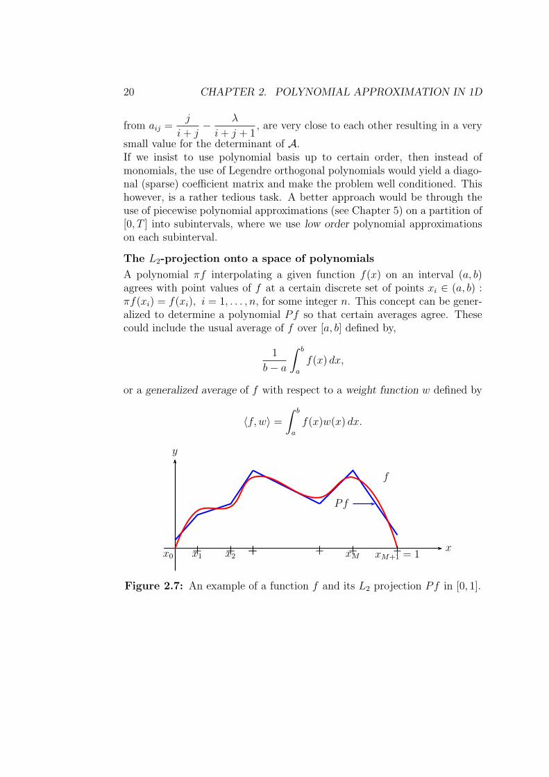
The L2-projection onto a space of polynomials
A polynomial πf interpolating a given function f(x) on an interval (a, b)agrees with point values of f at a certain discrete set of points xi ∈ (a, b) :πf(xi) = f(xi), i = 1, . . . , n, for some integer n. This concept can be gener-alized to determine a polynomial Pf so that certain averages agree. Thesecould include the usual average of f over [a, b] defined by,
1
b− a
∫ b
a
f(x) dx,
or a generalized average of f with respect to a weight function w defined by
〈f, w〉 =∫ b
a
f(x)w(x) dx.
x0 x2x1x
y
xM xM+1 = 1
f
Pf
Figure 2.7: An example of a function f and its L2 projection Pf in [0, 1].

2.4. A GALERKIN METHOD FOR (BVP) 21
Definition 2.8. The orthogonal projection, or L2-projection, of the functionf onto Pq(a, b) is the polynomial Pf ∈ Pq(a, b) such that
(f, w) = (Pf, w) ⇐⇒ (f − Pf, w) = 0 for all w ∈ Pq(a, b). (2.3.7)
Thus, (2.3.7) is equivalent to a (q + 1)× (q + 1) system of equations.
2.4 A Galerkin method for (BVP)
We consider Galerkin method for the following stationary (u = du/dt = 0)heat equation in one dimension:
−u′′(x) = f(x), 0 < x < 1; u(0) = u(1) = 0. (2.4.1)
Let Th : jhM+1j=0 , (M + 1)h = 1 be a uniform partition of the interval [0, 1]
into the subintervals Ij = ((j − 1)h, jh), with the same length |I| = h,j = 1, 2, . . . ,M + 1. We define the finite dimensional space V 0
h by
V 0h := v ∈ C(0, 1) : v is a piecewise linear function on Th, v(0) = v(1) = 0,
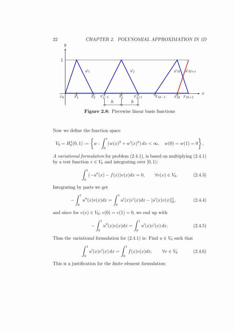
with the basis functions ϕjMj=1 defined below (these functions will be used todetermine the values of approximate solution at the points xj, j = 1, . . . ,M.Due to the fact that u is known at the boundary points 0 and 1; it is notnecessary to supply test functions corresponding to the values at x0 = 0 andxM+1 = 1. However, in the case of given non-homogeneous boundary datau(0) = u0 6= 0 and/or u(1) = u1 6= 0, to represent the trial function, one usesthe basis functions to all internal nodes as well as those corresponding to thenon-homogeneous data (i.e. at x = 0 and/or x = 1).
Remark 2.1. If the Dirichlet boundary condition is given at only one of theboundary points; say x0 = 0 and the other one satisfies, e.g. a Neumanncondition as
−u′′(x) = f(x), 0 < x < 1; u(0) = b0, u′(1) = b1, (2.4.2)
then the function ϕ0 (at x0 = 0 ) will be unnecessary (no matter whetherb0 = 0 or b0 6= 0), whereas one needs to provide the half-base function ϕM+1
at xM+1 = 1 (dashed in (2.8) below). Note that, ϕ0 participates (as data) inrepresenting the trial function U (see excercises at the end of this chapter).
22 CHAPTER 2. POLYNOMIAL APPROXIMATION IN 1D
x0 x1 x2
1
x
y
xj−1 xj xj+1 xM−1 xM xM+1
h h
ϕjϕ1 ϕM ϕM+1
Figure 2.8: Piecewise linear basis functions
Now we define the function space
V0 = H10 (0, 1) :=
w :
∫ 1
0
(w(x)2 + w′(x)2) dx <∞, w(0) = w(1) = 0
,
A variational formulation for problem (2.4.1), is based on multiplying (2.4.1)by a test function v ∈ V0 and integrating over [0, 1):
∫ 1
0
(−u′′(x)− f(x))v(x)dx = 0, ∀v(x) ∈ V0. (2.4.3)
Integrating by parts we get
−∫ 1
0
u′′(x)v(x)dx =
∫ 1
0
u′(x)v′(x)dx− [u′(x)v(x)]10, (2.4.4)
and since for v(x) ∈ V0; v(0) = v(1) = 0, we end up with
−∫ 1
0
u′′(x)v(x)dx =
∫ 1
0
u′(x)v′(x) dx. (2.4.5)
Thus the variational formulation for (2.4.1) is: Find u ∈ V0 such that
∫ 1
0
u′(x)v′(x) dx =
∫ 1
0
f(x)v(x)dx, ∀v ∈ V0 (2.4.6)
This is a justification for the finite element formulation:
2.4. A GALERKIN METHOD FOR (BVP) 23
The Galerkin finite element method (FEM) for the problem (2.4.1):Find U(x) ∈ V 0
h such that
∫ 1
0
U ′(x)v′(x) dx =
∫ 1
0
f(x)v(x)dx, ∀v(x) ∈ V 0h . (2.4.7)
Thus the Galerkin approximation U is very similar to Pu: The L2-projectionof u. We shall determine ξj = U(xj) which are the approximate values of u(x)at the node points xj = jh, 1 ≤ j ≤ M . To this end using basis functionsϕj(x), we may write
U(x) =M∑
j=1
ξj ϕj(x) which implies that U ′(x) =M∑
j=1
ξjϕ′j(x). (2.4.8)
Thus, (2.4.7) can be written as
M∑
j=1
ξj
∫ 1
0
ϕ′j(x) v
′(x)dx =
∫ 1
0
f(x)v(x)dx, ∀v(x) ∈ V 0h . (2.4.9)
Since every v(x) ∈ V 0h is a linear combination of the basis functions ϕi(x),
it suffices to try with v(x) = ϕi(x), for i = 1, 2, . . . ,M : That is, to find ξj(constants), 1 ≤ j ≤M such that
M∑
j=1
(∫ 1
0
ϕ′i(x)ϕ
′j(x)dx
)ξj =
∫ 1
0
f(x)ϕi(x)dx, i = 1, 2, . . . ,M. (2.4.10)
This M ×M system of equations can be written in the matrix form as
Aξ = b. (2.4.11)
Here A is called the stiffness matrix and b the load vector:
A = aijMi,j=1, aij =
∫ 1
0
ϕ′i(x)ϕ
′j(x)dx, (2.4.12)
b =
b1
b2
. . .
bM
, with bi =
∫ 1
0
f(x)ϕi(x)dx, and ξ =
ξ1
ξ2
. . .
ξM
. (2.4.13)

24 CHAPTER 2. POLYNOMIAL APPROXIMATION IN 1D
To compute the entries aij of the matrix A, first we need to derive ϕ′i(x), viz
ϕi(x) =
x−(i−1)hh
(i− 1)h ≤ x ≤ ih
(i+1)h−xh
ih ≤ x ≤ (i+ 1)h
0 else
ϕ′i(x) =
1h
(i− 1)h < x < ih
− 1h
ih < x < (i+ 1)h
0 else
Stiffness matrix A:
If |i− j| > 1, then ϕi and ϕj have disjoint support, see Figure 2.7, and
aij =
∫ 1
0
ϕ′i(x)ϕ
′j(x)dx = 0.
1
x
y
xj−2 xj−1 xj xj+1 xj+2
ϕj−1 ϕj+1
Figure 2.9: ϕj−1 and ϕj+1.
As for i = j: we have that
aii =
∫ xi
xi−1
(1h
)2
dx+
∫ xi+1
xi
(− 1
h
)2
dx =
h︷ ︸︸ ︷xi − xi−1
h2+
h︷ ︸︸ ︷xi+1 − xi
h2=
1
h+
1
h=
2
h.
2.4. A GALERKIN METHOD FOR (BVP) 25
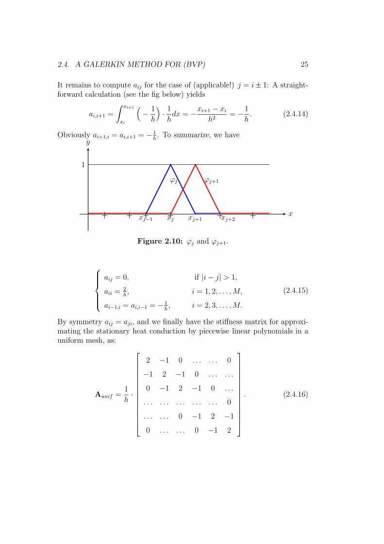
It remains to compute aij for the case of (applicable!) j = i± 1: A straight-forward calculation (see the fig below) yields
ai,i+1 =
∫ xi+1
xi
(− 1
h
)· 1hdx = −xi+1 − xi
h2= −1
h. (2.4.14)
Obviously ai+1,i = ai,i+1 = − 1h. To summarize, we have
1
x
y
xj−1 xj xj+1 xj+2
ϕj ϕj+1
Figure 2.10: ϕj and ϕj+1.
aij = 0, if |i− j| > 1,
aii =2h, i = 1, 2, . . . ,M,
ai−1,i = ai,i−1 = − 1h, i = 2, 3, . . . ,M.
(2.4.15)
By symmetry aij = aji, and we finally have the stiffness matrix for approxi-mating the stationary heat conduction by piecewise linear polynomials in auniform mesh, as:
Aunif =1
h·
2 −1 0 . . . . . . 0
−1 2 −1 0 . . . . . .
0 −1 2 −1 0 . . .
. . . . . . . . . . . . . . . 0
. . . . . . 0 −1 2 −1
0 . . . . . . 0 −1 2
. (2.4.16)

26 CHAPTER 2. POLYNOMIAL APPROXIMATION IN 1D
As for the components of the load vector b we have
bi =
∫ 1
0
f(x)ϕi(x) dx =
∫ xi
xi−1
f(x)x− xi−1
hdx+
∫ xi+1
xi
f(x)xi+1 − x
hdx.
2.4.1 The nonuniform version
Now let Th : 0 = x0 < x1 < . . . < xM < xM+1 = 1 be a partition ofthe interval (0, 1) into nonuniform subintervals Ij = (xj−1, xj), with lengths|Ij| = hj = xj − xj−1, j = 1, 2, . . . ,M + 1. We define the finite dimensionalspace V 0
h by
V 0h := v ∈ C(0, 1) : v is a piecewise linear function on Th, v(0) = v(1) = 0,
with the nonuniform basis functions ϕjMj=1. To compute the entries aij ofthe coefficient matrix A, first we need to derive ϕ′
i(x) for the nonuniformbasis functions: i.e.,
ϕi(x) =
x−xi−1
hixi−1 ≤ x ≤ xi
xi+1−xhi+1
xi ≤ x ≤ xi+1
0 else
=⇒
ϕ′i(x) =
1hi
xi−1 < x < xi
− 1hi+1
xi < x < xi+1
0 else
Nonuniform stiffness matrix A:If |i− j| > 1, then ϕi and ϕj have disjoint support, see Figure 2.9, and
aij =
∫ 1
0
ϕ′i(x)ϕ
′j(x)dx = 0.
As for i = j: we have that
aii =
∫ xi
xi−1
( 1
hi
)2
dx+
∫ xi+1
xi
(− 1
hi+1
)2
dx =
hi︷ ︸︸ ︷xi − xi−1
h2i+
hi+1︷ ︸︸ ︷xi+1 − xih2i+1
=1
hi+
1
hi+1
.
2.5. EXERCISES 27
For the case of (applicable!) j = i± 1:
ai,i+1 =
∫ xi+1
xi
(− 1
hi+1
)· 1
hi+1
dx = −xi+1 − xih2i+1
= − 1
hi+1
. (2.4.17)
Obviously ai+1,i = ai,i+1 = − 1hi+1
. Thus in nonuniform case we have that
aij = 0, if |i− j| > 1,
aii =1hi+ 1
hi+1, i = 1, 2, . . . ,M,
ai−1,i = ai,i−1 = − 1hi, i = 2, 3, . . . ,M.
(2.4.18)
By symmetry aij = aji, and we finally have the stiffness matrix in nonuniformmesh, for the stationary heat conduction as:
A =
1h1
+ 1h2
− 1h2
0 . . . 0
− 1h2
1h2
+ 1h3
− 1h3
0 0
0 . . . . . . . . . 0
. . . 0 . . . . . . − 1hM
0 . . . 0 − 1hM
1hM
+ 1hM+1
. (2.4.19)
With a uniform mesh, i.e. hi = h we get that A = Aunif .
Remark 2.2. Unlike the matrix A for polynomial approximation of IVP in(2.3.5), A has a more desirable structure, e.g. A is a sparse, tridiagonal andsymmetric matrix. This is due to the fact that the basis functions ϕjMj=1
are nearly orthogonal.
2.5 Exercises
Problem 2.1. Prove that V(q)0 := v ∈ P (q)(0, 1) : v(0) = 0, is a subspace
of P (q)(0, 1).
Problem 2.2. Consider the ODE: u(t) = u(t), 0 < t < 1; u(0) = 1.Compute its Galerkin approximation in P (q)(0, 1), for q = 1, 2, 3, and 4.

28 CHAPTER 2. POLYNOMIAL APPROXIMATION IN 1D
Problem 2.3. Consider the ODE: u(t) = u(t), 0 < t < 1; u(0) = 1.Compute the L2(0, 1) projection of the exact solution u into P3(0, 1).
Problem 2.4. Compute the stiffness matrix and load vector in a finite ele-ment approximation of the boundary value problem
−u′′(x) = f(x), 0 < x < 1, u(0) = u(1) = 0,
with f(x) = x and h = 1/4.
Problem 2.5. We want to find a solution approximation U(x) to
−u′′(x) = 1, 0 < x < 1, u(0) = u(1) = 0,
using the ansatz U(x) = A sin πx+B sin 2πx.
a. Calculate the exact solution u(x).
b. Write down the residual R(x) = −U ′′(x)− 1
c. Use the orthogonality condition
∫ 1
0
R(x) sin πnx dx = 0, n = 1, 2,
to determine the constants A and B.
d. Plot the error e(x) = u(x)− U(x).
Problem 2.6. Consider the boundary value problem
−u′′(x) + u(x) = x, 0 < x < 1, u(0) = u(1) = 0.
a. Verify that the exact solution of the problem is given by
u(x) = x− sinh x
sinh 1.
b. Let U(x) be a solution approximation defined by
U(x) = A sin πx+ B sin 2πx+ C sin 3πx,
where A, B, and C are unknown constants. Compute the residual function
R(x) = −U ′′(x) + U(x)− x.
2.5. EXERCISES 29
c. Use the orthogonality condition
∫ 1
0
R(x) sin πnx dx = 0, n = 1, 2, 3,
to determine the constants A, B, and C.
Problem 2.7. Let U(x) = ξ0φ0(x) + ξ1φ1(x) be a solution approximation to
−u′′(x) = x− 1, 0 < x < π, u′(0) = u(π) = 0,
where ξi, i = 0, 1, are unknown coefficients and
φ0(x) = cosx
2, φ1(x) = cos
3x
2.
a. Find the analytical solution u(x).
b. Define the approximate solution residual R(x).
c. Compute the constants ξi using the orthogonality condition
∫ π
0
R(x)φi(x) dx = 0, i = 0, 1,
i.e., by approximating u(x) as a linear combination of φ0(x) and φ1(x)
Problem 2.8. Use the projection technique of the previous exercises to solve
−u′′(x) = 0, 0 < x < π, u(0) = 0, u(π) = 2,
assuming that U(x) = A sin x+ B sin 2x+ C sin 3x+ 2π2x
2.
Problem 2.9. Show that (f − Phf, v) = 0, ∀v ∈ Vh, if and only if (f −Phf, ϕi) = 0, i = 0, . . . , N ; where ϕiNi=1 ⊂ Vh is the basis of hat-functions.

30 CHAPTER 2. POLYNOMIAL APPROXIMATION IN 1D

Chapter 3
Interpolation, NumericalIntegration in 1d
3.1 Preliminaries
Definition 3.1. A polynomial interpolant πqf of a function f , defined onan interval I = [a, b], is a polynomial of degree ≤ q having the nodal valuesat q + 1 distinct points xj ∈ [a, b], j = 0, 1, . . . , q, coinciding with those of f ,i.e., πqf ∈ Pq(a, b) and πqf(xj) = f(xj), j = 0, . . . , q.
Below we illustrate this definition through a simple and familiar example.
Example 3.1. Linear interpolation on an interval. We start with theunit interval I := [0, 1] and a continuous function f : I → R. We let q = 1and seek the linear interpolant of f on I, i.e. the linear function π1f ∈ P1,such that π1f(0) = f(0) and π1f(1) = f(1). Thus we seek the constants C0
and C1 in the following representation of π1f ∈ P1,
π1f(x) = C0 + C1x, x ∈ I, (3.1.1)
where
π1f(0) = f(0) =⇒ C0 = f(0), and
π1f(1) = f(1) =⇒ C0 + C1 = f(1) =⇒ C1 = f(1)− f(0).(3.1.2)
Inserting C0 and C1 into (3.1.1) it follows that
π1f(x) = f(0)+(f(1)−f(0))x = f(0)(1−x)+f(1)x := f(0)λ0(x)+f(1)λ1(x).
31

32CHAPTER 3. INTERPOLATION, NUMERICAL INTEGRATION IN 1D
In other words π1f(x) is represented in two different bases:
π1f(x) = C0 · 1 + C1 · x, with 1, x as the set of basis functions and
π1f(x) = f(0)(1−x)+f(1)x, with 1−x, x as the set of basis functions.
The functions λ0(x) = 1− x and λ1(x) = x are linearly independent, since if
0 = α0(1− x) + α1x = α0 + (α1 − α0)x, for all x ∈ I, (3.1.3)
thenx = 0 =⇒ α0 = 0
x = 1 =⇒ α1 = 0
=⇒ α0 = α1 = 0. (3.1.4)
1
f(x)
π1f(x)
1
λ0(x) = 1− x1
λ1(x) = x
Figure 3.1: Linear interpolation and basis functions for q = 1.
Remark 3.1. Note that if we define a scalar product on Pk(a, b) by
(p, q) =
∫ b
a
p(x)q(x) dx, ∀p, q ∈ Pk(a, b), (3.1.5)
then we can easily verify that neither 1, x nor 1− x, x is an orthogonal
basis for P1(0, 1), since (1, x) :=∫ 1
01 · x dx = [x
2
2] = 1
26= 0 and (1− x, x) :=∫ 1
0(1− x)x dx = 1
66= 0.
With such background, it is natural to pose the following question:

3.1. PRELIMINARIES 33
Question 3.1. How well does πqf approximate f? In other words howlarge/small will the error be in approximating f(x) by πqf(x)?
To answer this question we need to estimate the difference between f(x) andπqf(x). For instance for q = 1, geometrically, the deviation of f(x) fromπ1f(x) (from being linear) depends on the curvature of f(x), i.e. on howcurved f(x) is. In other words, on how large f ′′(x) is, say, on an interval(a, b). To quantify the relationship between the size of the error f −π1f andthe size of f ′′, we need to introduce some measuring instrument for vectorsand functions:
Definition 3.2. Let x = (x1, . . . , xn)T and y = (y1, . . . , yn)
T ∈ Rn be twocolumn vectors (T stands for transpose). We define the scalar product of xand y by
〈x,y〉 = xTy = x1y1 + · · ·+ xnyn,
and the vector norm for x as the Euclidean length of x:
‖x‖ :=√〈x,x〉 =
√x21 + · · ·+ x2n.
Lp(a, b)-norm: Assume that f is a real valued function defined on the in-terval (a, b). Then we define the Lp-norm (1 ≤ p ≤ ∞) of f by
Lp-norm ‖f‖Lp(a,b) :=(∫ b
a
|f(x)|pdx)1/p
, 1 ≤ p <∞,
L∞-norm ‖f‖L∞(a,b) := maxx∈[a,b]
|f(x)|.
For 1 ≤ p ≤ ∞ we define the Lp(a, b)-space by
Lp(a, b) := f : ‖f‖Lp(a,b) <∞.
Below we shall answer Question 3.1, first in the L∞-norm, and then in theLp-norm (mainly for p = 1, 2.)
Theorem 3.1. (L∞-error estimates for linear interpolation in an interval)Assume that f ′′ ∈ L∞(a, b). Then, for q = 1, i.e. only 2 interpolationnodes (e.g. end-points of the interval), there are interpolation constants,Ci, i = 1, 2, 3., independent of the function f and the size of the interval[a, b], such that
(1) ‖π1f − f‖L∞(a,b) ≤ C1(b− a)2‖f ′′‖L∞(a,b)
34CHAPTER 3. INTERPOLATION, NUMERICAL INTEGRATION IN 1D
(2) ‖π1f − f‖L∞(a,b) ≤ C2(b− a)‖f ′‖L∞(a,b)
(3) ‖(π1f)′ − f ′‖L∞(a,b) ≤ C3(b− a)‖f ′′‖L∞(a,b).
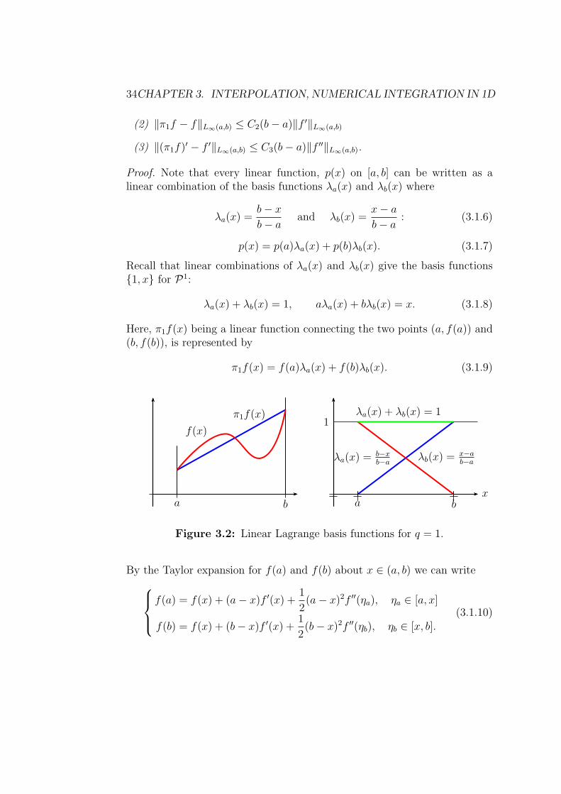
Proof. Note that every linear function, p(x) on [a, b] can be written as alinear combination of the basis functions λa(x) and λb(x) where
λa(x) =b− x
b− aand λb(x) =
x− a
b− a: (3.1.6)
p(x) = p(a)λa(x) + p(b)λb(x). (3.1.7)
Recall that linear combinations of λa(x) and λb(x) give the basis functions1, x for P1:
λa(x) + λb(x) = 1, aλa(x) + bλb(x) = x. (3.1.8)
Here, π1f(x) being a linear function connecting the two points (a, f(a)) and(b, f(b)), is represented by
π1f(x) = f(a)λa(x) + f(b)λb(x). (3.1.9)
1
a
π1f(x)
b
f(x)
a bx
λa(x) =b−xb−a
λb(x) =x−ab−a
λa(x) + λb(x) = 1
Figure 3.2: Linear Lagrange basis functions for q = 1.
By the Taylor expansion for f(a) and f(b) about x ∈ (a, b) we can write
f(a) = f(x) + (a− x)f ′(x) +1
2(a− x)2f ′′(ηa), ηa ∈ [a, x]
f(b) = f(x) + (b− x)f ′(x) +1
2(b− x)2f ′′(ηb), ηb ∈ [x, b].
(3.1.10)
3.1. PRELIMINARIES 35
Inserting f(a) and f(b) from (3.1.10) into (3.1.9), it follows that
π1f(x) =[f(x) + (a− x)f ′(x) +1
2(a− x)2f ′′(ηa)]λa(x)+
+[f(x) + (b− x)f ′(x) +1
2(b− x)2f ′′(ηb)]λb(x).
Rearranging the terms, using (3.1.8) and the identity (which also followsfrom (3.1.8)) (a− x)λa(x) + (b− x)λb(x) = 0 we get
π1f(x) = f(x)[λa(x) + λb(x)] + f ′(x)[(a− x)λa(x) + (b− x)λb(x)]+
+1
2(a− x)2f ′′(ηa)λa(x) +
1
2(b− x)2f ′′(ηb)λb(x) =
= f(x) +1
2(a− x)2f ′′(ηa)λa(x) +
1
2(b− x)2f ′′(ηb)λb(x).
Consequently
|π1f(x)− f(x)| =∣∣∣1
2(a− x)2f ′′(ηa)λa(x) +
1
2(b− x)2f ′′(ηb)λb(x)
∣∣∣. (3.1.11)
To proceed, we note that for a ≤ x ≤ b both (a−x)2 ≤ (a−b)2 and (b−x)2 ≤(a − b)2, furthermore λa(x) ≤ 1 and λb(x) ≤ 1, ∀ x ∈ (a, b). Moreover,by the definition of the maximum norm both |f ′′(ηa)| ≤ ‖f ′′‖L∞(a,b), and|f ′′(ηb)| ≤ ‖f ′′‖L∞(a,b). Thus we may estimate (3.1.11) as
|π1f(x)−f(x)| ≤1
2(a−b)2 ·1 ·‖f ′′‖L∞(a,b)+
1
2(a−b)2 ·1 ·‖f ′′‖L∞(a,b), (3.1.12)
and hence
|π1f(x)−f(x)| ≤ (a−b)2‖f ′′‖L∞(a,b) corresponding to ci = 1. (3.1.13)
The other two estimates (2) and (3) are proved similarly.
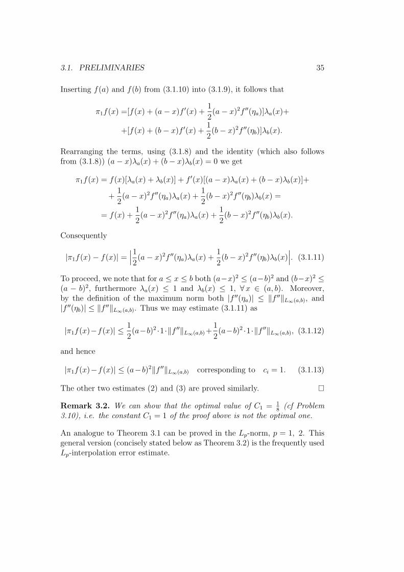
Remark 3.2. We can show that the optimal value of C1 = 18(cf Problem
3.10), i.e. the constant C1 = 1 of the proof above is not the optimal one.
An analogue to Theorem 3.1 can be proved in the Lp-norm, p = 1, 2. Thisgeneral version (concisely stated below as Theorem 3.2) is the frequently usedLp-interpolation error estimate.

36CHAPTER 3. INTERPOLATION, NUMERICAL INTEGRATION IN 1D
Theorem 3.2. Let π1v(x) be the linear interpolant of the function v(x) on(a, b). Then, assuming that v is twice differentiable (v ∈ C2(a, b)), there areinterpolation constants ci, i = 1, 2, 3 such that for p = 1, 2, ∞,
‖π1v − v‖Lp(a,b) ≤ c1(b− a)2‖v′′‖Lp(a,b), (3.1.14)
‖(π1v)′ − v′‖Lp(a,b) ≤ c2(b− a)‖v′′‖Lp(a,b), (3.1.15)
‖π1v − v‖Lp(a,b) ≤ c3(b− a)‖v′‖Lp(a,b). (3.1.16)
For p = ∞ this is just the previous Theorem 3.1.
Proof. For p = 1 and p = 2, the proof uses the integral form of the Taylorexpansion and is left as an exercise.
Below we review a simple piecewise linear interpolation procedure on apartition of an interval:
Vector space of piecewise linear functions on an interval. GivenI = [a, b], let Th : a = x0 < x1 < x2 < . . . < xN−1 < xN = b be apartition of I into subintervals Ij = [xj−1, xj] of length hj = |Ij| := xj−xj−1;j = 1, 2, . . . , N . Let
Vh := v|v is a continuous, piecewise linear function on Th, (3.1.17)
then Vh is a vector space with the previously introduced hat functions:ϕjNj=0 as basis functions. Note that ϕ0(x) and ϕN(x) are left and righthalf-hat functions, respectively. We now show that every function in Vh is alinear combination of ϕj:s.
Lemma 3.1. We have that
∀v ∈ Vh; v(x) =N∑
j=0
v(xj)ϕj(x). (3.1.18)
Proof. Both the left and right hand side are continuous piecewise linear func-tions. Thus it suffices to show that they have the same nodal values: Letx = xj, then since ϕi(xj) = δij,
RHS|xj=v(x0)ϕ0(xj) + v(x1)ϕ1(xj) + . . .+ v(xj−1)ϕj−1(xj)
+ v(xj)ϕj(xj) + v(xj+1)ϕj+1(xj) + . . .+ v(xN)ϕN(xj)
=v(xj) = LHS|xj.
(3.1.19)

3.1. PRELIMINARIES 37
Definition 3.3. For a partition Th : a = x0 < x1 < x2 < . . . < xN = b ofthe interval [a, b] we define the mesh function h(x) as the piecewise constantfunction h(x) := hj = xj − xj−1 for x ∈ Ij = (xj−1, xj), j = 1, 2, . . . , N .
Definition 3.4. Assume that f is a continuous function in [a, b]. Then thecontinuous piecewise linear interpolant of f is defined by
πhf(x) =N∑
j=0
f(xj)ϕj(x), x ∈ [a, b].
Here the sub-index h refers to the mesh function h(x).
Hence
πhf(xj) = f(xj), j = 0, 1, . . . , N. (3.1.20)
Remark 3.3. Note that we denote the linear interpolant, defined for a singleinterval [a, b], by π1f which is a polynomial of degree 1, whereas the piecewiselinear interpolant πhf is defined for a partition Th of [a, b] and is a piecewiselinear function. For the piecewise polynomial interpolants of (higher) degreeq we shall use the notation for Cardinal functions of Lagrange interpolation(see Section 3.2).
Note that for each interval Ij, j = 1, . . . , N , we have that
(i) πhf(x) is linear on Ij =⇒ πhf(x) = c0 + c1x for x ∈ Ij.
(ii) πhf(xj−1) = f(xj−1) and πhf(xj) = f(xj).
Combining (i) and (ii) we get
πhf(xj−1) = c0 + c1xj−1 = f(xj−1)
πhf(xj) = c0 + c1xj = f(xj)=⇒
c1 =f(xj)−f(xj−1)
xj−xj−1
c0 =−xj−1f(xj)+xjf(xj−1)
xj−xj−1.
Thus, we may write
c0 = f(xj−1)xj
xj−xj−1+ f(xj)
−xj−1
xj−xj−1
c1x = f(xj−1)−x
xj−xj−1+ f(xj)
xxj−xj−1
.(3.1.21)
38CHAPTER 3. INTERPOLATION, NUMERICAL INTEGRATION IN 1D
x0 x1 x2
f(x)πhf(x)
xj xN−1 xNx
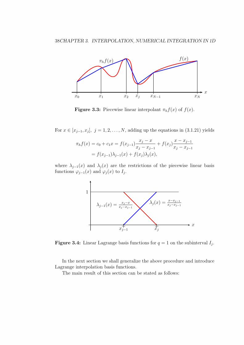
Figure 3.3: Piecewise linear interpolant πhf(x) of f(x).
For x ∈ [xj−1, xj ], j = 1, 2, . . . , N , adding up the equations in (3.1.21) yields
πhf(x) = c0 + c1x = f(xj−1)xj − x
xj − xj−1
+ f(xj)x− xj−1
xj − xj−1
= f(xj−1)λj−1(x) + f(xj)λj(x),
where λj−1(x) and λj(x) are the restrictions of the piecewise linear basisfunctions ϕj−1(x) and ϕj(x) to Ij.
1
xj−1 xjx
λj−1(x) =xj−x
xj−xj−1
λj(x) =x−xj−1
xj−xj−1
Figure 3.4: Linear Lagrange basis functions for q = 1 on the subinterval Ij.
In the next section we shall generalize the above procedure and introduceLagrange interpolation basis functions.
The main result of this section can be stated as follows:
3.2. LAGRANGE INTERPOLATION 39
Theorem 3.3. Let πhv(x) be the piecewise linear interpolant of the functionv(x) on the partition Th of [a, b]. Then assuming that v is sufficiently regular(v ∈ C2(a, b)), there are interpolation constants ci, i = 1, 2, 3, such that forp = 1, 2, ∞,
‖πhv − v‖Lp(a,b) ≤ c1‖h2v′′‖Lp(a,b), (3.1.22)
‖(πhv)′ − v′‖Lp(a,b) ≤ c2‖hv′′‖Lp(a,b), (3.1.23)
‖πhv − v‖Lp(a,b) ≤ c3‖hv′‖Lp(a,b). (3.1.24)
Proof. Recalling the definition of the partition Th, we may write
‖πhv − v‖pLp(a,b)=
N∑
j=1
‖πhv − v‖pLp(Ij)≤
N∑
j=1
cp1‖h2jv′′‖pLp(Ij)
≤ cp1‖h2v′′‖pLp(a,b),
(3.1.25)
where in the first inequality we apply Theorem 3.2 to an arbitrary partitioninterval Ij and them sum over j. The other two estimates are proved similarly.
3.2 Lagrange interpolation
Consider Pq(a, b); the vector space of all polynomials of degree ≤ q on theinterval (a, b), with the basis functions 1, x, x2, . . . , xq. We have seen, inChapter 2, that this is a non-orthogonal basis (with respect to scalar product(3.1.5) with, e.g. a = 0 and b = 1) that leads to ill-conditioned coefficientmatrices. We will now introduce a new set of basis functions, which beingalmost orthogonal have some useful properties.
Definition 3.5 (Cardinal functions). Lagrange basis is the set of polynomialsλiqi=0 ⊂ P q(a, b) associated with the (q + 1) distinct points, a = x0 < x1 <. . . < xq = b in [a, b] and determined by the requirement that: at the nodes,λi(xj) = 1 for i = j, and 0 otherwise (λi(xj) = 0 for i 6= j), i.e. for x ∈ [a, b],
λi(x) =(x− x0)(x− x1) . . . (x− xi−1) ↓ (x− xi+1) . . . (x− xq)
(xi − x0)(xi − x1) . . . (xi − xi−1) ↑ (xi − xi+1) . . . (xi − xq). (3.2.1)
40CHAPTER 3. INTERPOLATION, NUMERICAL INTEGRATION IN 1D
By the arrows ↓ , ↑ in (3.2.1) we want to emphasize that λi(x) =∏
j 6=i
( x− xjxi − xj
)
does not contain the singular factorx− xixi − xi
. Hence
λi(xj) =(xj − x0)(xj − x1) . . . (xj − xi−1)(xj − xi+1) . . . (xj − xq)
(xi − x0)(xi − x1) . . . (xi − xi−1)(xi − xi+1) . . . (xi − xq)= δij,
and λi(x), i = 0, 1, . . . , q, is a polynomial of degree q on (a, b) with
λi(xj) = δij =
1 i = j
0 i 6= j.(3.2.2)
Example 3.2. Let q = 2, then we have a = x0 < x1 < x2 = b, where
i = 1, j = 2 ⇒ λ1(x2) =(x2 − x0)(x2 − x2)
(x1 − x0)(x1 − x2)= 0
i = j = 1 ⇒ λ1(x1) =(x1 − x0)(x1 − x2)
(x1 − x0)(x1 − x2)= 1.
A polynomial P (x) ∈ Pq(a, b) with the values pi = P (xi) at the nodes xi,i = 0, 1, . . . , q, can be expressed in terms of the above Lagrange basis as
P (x) = p0λ0(x) + p1λ1(x) + . . .+ pqλq(x). (3.2.3)
Using (3.2.2), P (xi) = p0λ0(xi)+p1λ1(xi)+. . .+piλi(xi)+. . .+pqλq(xi) = pi.Recalling definition 3.1, if we choose a ≤ ξ0 < ξ1 < . . . < ξq ≤ b, as
q+1 distinct interpolation nodes on [a, b], then the interpolating polynomialπqf ∈ Pq(a, b) satisfies
πqf(ξi) = f(ξi), i = 0, 1, . . . , q (3.2.4)
and the Lagrange formula (3.2.3) for πqf(x) reads as
πqf(x) = f(ξ0)λ0(x) + f(ξ1)λ1(x) + . . .+ f(ξq)λq(x), a ≤ x ≤ b.
Example 3.3. For q = 1, we have only the nodes a and b. Recall that
λa(x) =b− x
b− aand λb(x) =
x− a
b− a, thus as in the introduction in this chapter
π1f(x) = f(a)λa(x) + f(b)λb(x). (3.2.5)
3.3. NUMERICAL INTEGRATION, QUADRATURE RULES 41
Example 3.4. To interpolate f(x) = x3 + 1 by piecewise polynomials ofdegree 2, in the partition x0 = 0, x1 = 1, x2 = 2 of the interval [0, 2], wehave
π2f(x) = f(0)λ0(x) + f(1)λ1(x) + f(2)λ2(x),
where f(0) = 1, f(1) = 2, f(2) = 9, and we may compute Lagrange basis as
λ0(x) =1
2(x− 1)(x− 2), λ1(x) = −x(x− 2), λ2(x) =
1
2x(x− 1).
This yields
π2f(x) = 1 · 12(x− 1)(x− 2)− 2 · x(x− 2) + 9 · 1
2x(x− 1) = 3x2 − 2x+ 1.
3.3 Numerical integration, Quadrature rules
In the finite element approximation procedure of solving differential equa-tions, with a given source term (data) f(x), we need to evaluate integralsof the form
∫f(x)ϕi(x) dx, with ϕi(x) being a finite element basis function.
Such integrals are not easily computable for higher order approximations(e.g. with ϕi:s being Lagrange basis of high order) and more involved data.Further, we encounter matrices with entries being the integrals of productsof these, higher order, basis functions and their derivatives. Except somespecial cases (see calculations for A and Aunif in the previous chapter), suchintegrations are usually performed approximately by using numerical meth-ods. Below we briefly review some of these numerical integration techniques.
We approximate the integral I =∫ b
af(x)dx using a partition of the in-
terval [a, b] into subintervals, where on each subinterval f is approximatedby polynomials of a certain degree d. We shall denote the approximate valueof the integral I by Id. To proceed we assume, without loss of generality,that f(x) > 0 on [a, b] and that f is continuous on (a, b). Then the inte-
gral I =∫ b
af(x)dx is interpreted as the area of the domain under the curve
y = f(x); limited by the x-axis and the lines x = a and x = b. We shallapproximate this area using the values of f at certain points as follows.
We start by approximating the integral over a single interval [a, b]. Theserules are referred to as simple rules.
i) Simple midpoint rule uses the value of f at the midpoint x := a+b2
of [a, b],
i.e. f(
a+b2
). This means that f is approximated by the constant function

42CHAPTER 3. INTERPOLATION, NUMERICAL INTEGRATION IN 1D
(polynomial of degree 0) P0(x) = f(
a+b2
)and the area under the curve
y = f(x) by
I =
∫ b
a
f(x)dx ≈ (b− a)f(a+ b
2
). (3.3.1)
To prepare for generalizations, if we let x0 = a and x1 = b and assume thatthe length of the interval is h, then
I ≈ I0 = hf(a+
h
2
)= hf(x) (3.3.2)
a = x0
f(b)
a+ h/2 b = x1
f(a)
P0(x)f(a+ h/2)
x
Figure 3.5: Midpoint approximation I0 of the integral I =∫ x1
x0f(x)dx.
ii) Simple trapezoidal rule uses the values of f at two endpoints a and b, i.e.f(a) and f(b). Here f is approximated by the linear function (polynomial
of degree 1) P1(x) passing through the two points(a, f(a)
)and
(b, f(b)
).
Consequently, the area under the curve y = f(x) is approximated as
I =
∫ b
a
f(x)dx ≈ (b− a)f(a) + f(b)
2. (3.3.3)
This is the area of the trapezoidal between the lines y = 0, x = a andx = b and under the graph of P1(x), and therefore is referred to as the simpletrapezoidal rule. Once again, for the purpose of generalization, we let x0 = a,x1 = b and assume that the length of the interval is h, then (3.3.3) can be

3.3. NUMERICAL INTEGRATION, QUADRATURE RULES 43
written as
I ≈ I1 =hf(a) +h[f(a+ h)− f(a)]
2= h
f(a) + f(a+ h)
2
≡h2[f(x0) + f(x1)].
(3.3.4)
iii) Simple Simpson’s rule uses the values of f at the two endpoints a and b,
a = x0
f(b)P1(x)
b = x1 = a+ h
f(a)
x
Figure 3.6: Trapezoidal approximation I1 of the integral I =∫ x1
x0f(x)dx.
and the midpoint a+b2
of the interval [a, b], i.e. f(a), f(b), and f(
a+b2
). In this
case the area under y = f(x) is approximated by the area under the graph of
the second degree polynomial P2(x); with P2(a) = f(a), P2
(a+b2
)= f
(a+b2
),
and P2(b) = f(b). To determine P2(x) we may use Lagrange interpolationfor q = 2: let x0 = a, x1 = (a+ b)/2 and x2 = b, then
P2(x) = f(x0)λ0(x) + f(x1)λ1(x) + f(x2)λ2(x), (3.3.5)
where
λ0(x) =(x−x1)(x−x2)
(x0−x1)(x0−x2),
λ1(x) =(x−x0)(x−x2)
(x1−x0)(x1−x2),
λ2(x) =(x−x0)(x−x1)
(x2−x0)(x2−x1).
(3.3.6)
Thus
I =
∫ b
a
f(x)dx ≈∫ b
a
P2(x) dx =2∑
i=0
f(xi)
∫ b
a
λi(x) dx. (3.3.7)
44CHAPTER 3. INTERPOLATION, NUMERICAL INTEGRATION IN 1D
Now we can easily compute the integrals
∫ b
a
λ0(x) dx =
∫ b
a
λ2(x) dx =b− a
6,
∫ b
a
λ1(x) dx =4(b− a)
6. (3.3.8)
Hence
I =
∫ b
a
f(x)dx ≈ I2 =b− a
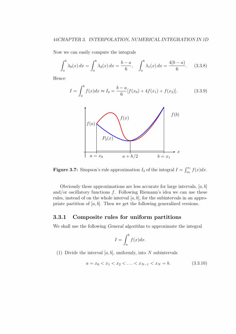
6[f(x0) + 4f(x1) + f(x2)]. (3.3.9)
a = x0
f(b)
a+ h/2 b = x1
f(x)
P2(x)
f(a)
x
Figure 3.7: Simpson’s rule approximation I2 of the integral I =∫ x1
x0f(x)dx.
Obviously these approximations are less accurate for large intervals, [a, b]and/or oscillatory functions f . Following Riemann’s idea we can use theserules, instead of on the whole interval [a, b], for the subintervals in an appro-priate partition of [a, b]. Then we get the following generalized versions.
3.3.1 Composite rules for uniform partitions
We shall use the following General algorithm to approximate the integral
I =
∫ b
a
f(x)dx.
(1) Divide the interval [a, b], uniformly, into N subintervals
a = x0 < x1 < x2 < . . . < xN−1 < xN = b. (3.3.10)
3.3. NUMERICAL INTEGRATION, QUADRATURE RULES 45
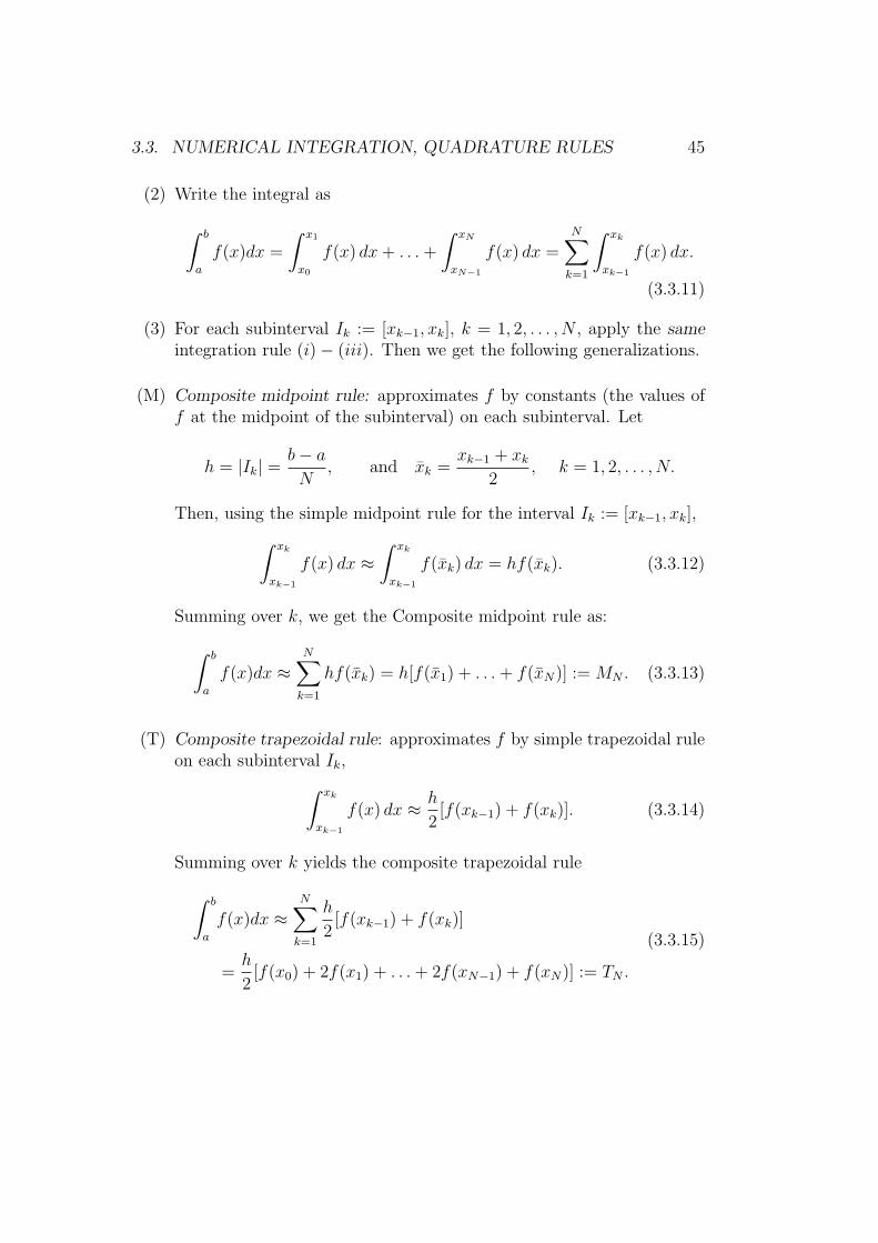
(2) Write the integral as
∫ b
a
f(x)dx =
∫ x1
x0
f(x) dx+ . . .+
∫ xN
xN−1
f(x) dx =N∑
k=1
∫ xk
xk−1
f(x) dx.
(3.3.11)
(3) For each subinterval Ik := [xk−1, xk], k = 1, 2, . . . , N , apply the sameintegration rule (i)− (iii). Then we get the following generalizations.
(M) Composite midpoint rule: approximates f by constants (the values off at the midpoint of the subinterval) on each subinterval. Let
h = |Ik| =b− a
N, and xk =
xk−1 + xk2
, k = 1, 2, . . . , N.
Then, using the simple midpoint rule for the interval Ik := [xk−1, xk],
∫ xk
xk−1
f(x) dx ≈∫ xk
xk−1
f(xk) dx = hf(xk). (3.3.12)
Summing over k, we get the Composite midpoint rule as:
∫ b
a
f(x)dx ≈N∑
k=1
hf(xk) = h[f(x1) + . . .+ f(xN)] :=MN . (3.3.13)
(T) Composite trapezoidal rule: approximates f by simple trapezoidal ruleon each subinterval Ik,
∫ xk
xk−1
f(x) dx ≈ h
2[f(xk−1) + f(xk)]. (3.3.14)
Summing over k yields the composite trapezoidal rule
∫ b
a
f(x)dx ≈N∑
k=1
h
2[f(xk−1) + f(xk)]
=h
2[f(x0) + 2f(x1) + . . .+ 2f(xN−1) + f(xN)] := TN .
(3.3.15)
46CHAPTER 3. INTERPOLATION, NUMERICAL INTEGRATION IN 1D
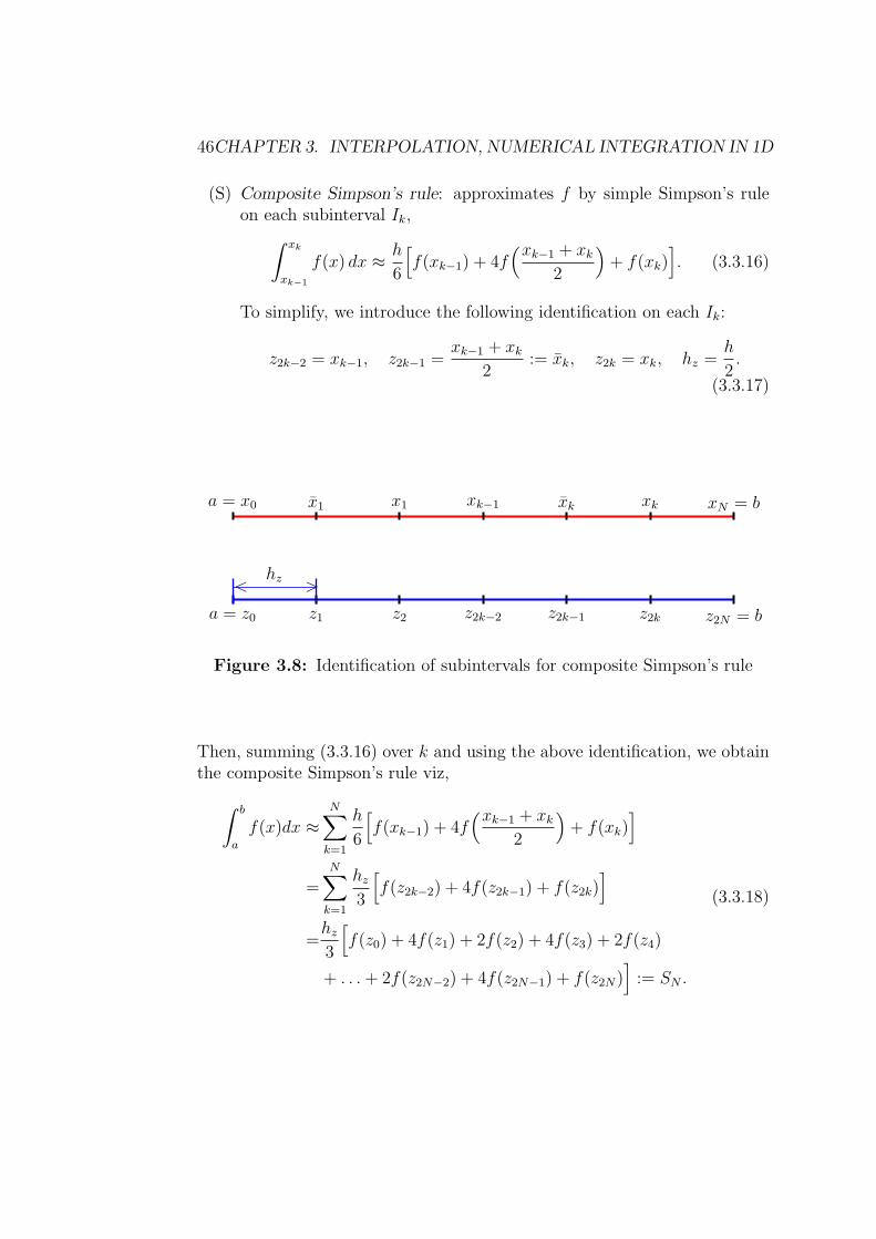
(S) Composite Simpson’s rule: approximates f by simple Simpson’s ruleon each subinterval Ik,
∫ xk
xk−1
f(x) dx ≈ h
6
[f(xk−1) + 4f
(xk−1 + xk2
)+ f(xk)
]. (3.3.16)
To simplify, we introduce the following identification on each Ik:
z2k−2 = xk−1, z2k−1 =xk−1 + xk
2:= xk, z2k = xk, hz =
h
2.
(3.3.17)
< >
a = z0
a = x0
z1
x1
z2
x1
z2k−2
xk−1
z2k−1
xk
z2k
xk
z2N = b
xN = b
hz
Figure 3.8: Identification of subintervals for composite Simpson’s rule
Then, summing (3.3.16) over k and using the above identification, we obtainthe composite Simpson’s rule viz,
∫ b
a
f(x)dx ≈N∑
k=1
h
6
[f(xk−1) + 4f
(xk−1 + xk2
)+ f(xk)
]
=N∑
k=1
hz3
[f(z2k−2) + 4f(z2k−1) + f(z2k)
]
=hz3
[f(z0) + 4f(z1) + 2f(z2) + 4f(z3) + 2f(z4)
+ . . .+ 2f(z2N−2) + 4f(z2N−1) + f(z2N)]:= SN .
(3.3.18)
3.3. NUMERICAL INTEGRATION, QUADRATURE RULES 47
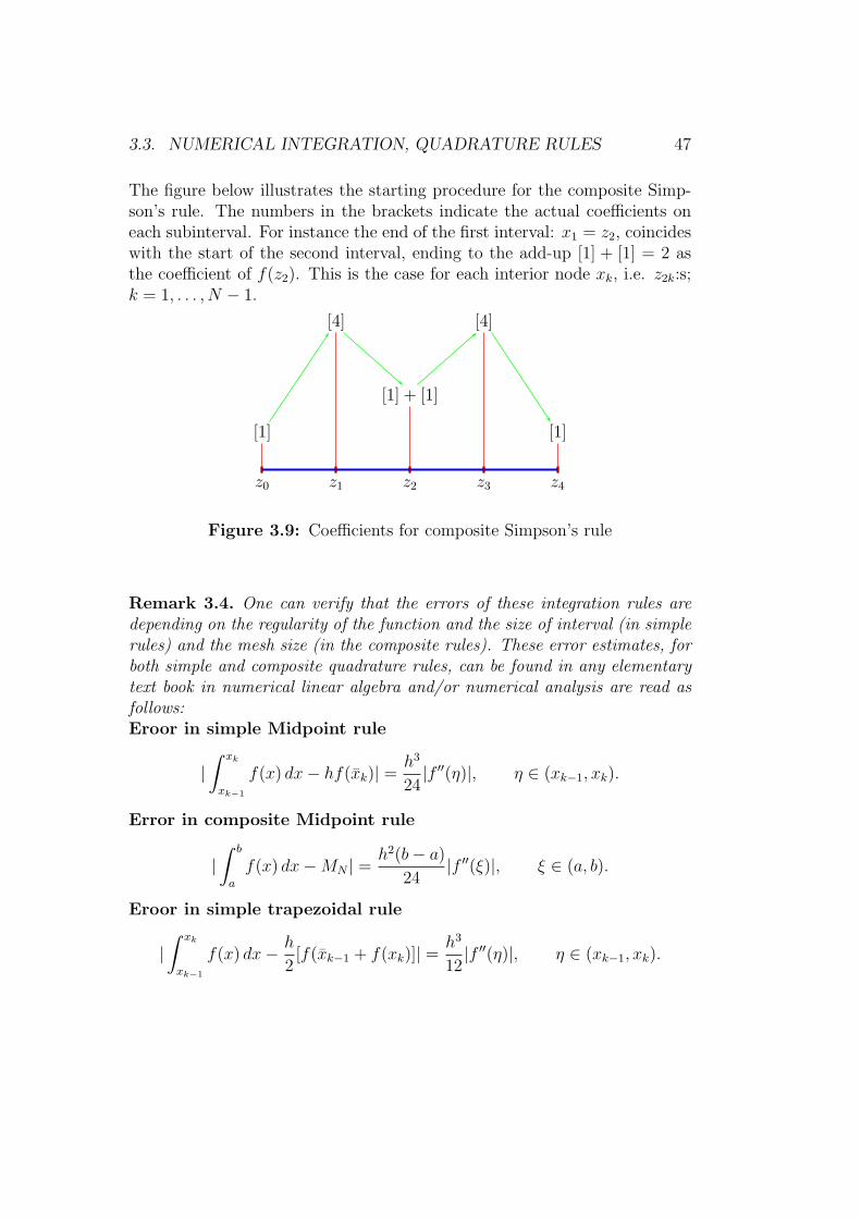
The figure below illustrates the starting procedure for the composite Simp-son’s rule. The numbers in the brackets indicate the actual coefficients oneach subinterval. For instance the end of the first interval: x1 = z2, coincideswith the start of the second interval, ending to the add-up [1] + [1] = 2 asthe coefficient of f(z2). This is the case for each interior node xk, i.e. z2k:s;k = 1, . . . , N − 1.
z0
[1]
z1
[4]
z2
[1] + [1]
z3
[4]
z4
[1]
Figure 3.9: Coefficients for composite Simpson’s rule
Remark 3.4. One can verify that the errors of these integration rules aredepending on the regularity of the function and the size of interval (in simplerules) and the mesh size (in the composite rules). These error estimates, forboth simple and composite quadrature rules, can be found in any elementarytext book in numerical linear algebra and/or numerical analysis are read asfollows:Eroor in simple Midpoint rule
|∫ xk
xk−1
f(x) dx− hf(xk)| =h3
24|f ′′(η)|, η ∈ (xk−1, xk).
Error in composite Midpoint rule
|∫ b
a
f(x) dx−MN | =h2(b− a)
24|f ′′(ξ)|, ξ ∈ (a, b).
Eroor in simple trapezoidal rule
|∫ xk
xk−1
f(x) dx− h
2[f(xk−1 + f(xk)]| =
h3
12|f ′′(η)|, η ∈ (xk−1, xk).
48CHAPTER 3. INTERPOLATION, NUMERICAL INTEGRATION IN 1D
Error in composite trapezoidal rule
|∫ b
a
f(x) dx− TN | =h2(b− a)
12|f ′′(ξ)|, ξ ∈ (a, b).
Eroor in simple Simpson’s rule
|∫ b
a
f(x) dx−b− a
6[f(a)+4f((a+b)/2)+f(b)]| = 1
90
(b− a
2
)5
|f (4)(η)|, η ∈ (a, b).
Error in composite Simpson’s rule
|∫ b
a
f(x) dx− SN | =h4(b− a)
180maxξ∈[a,b]
|f 4(ξ)|, h = (b− a)/N.
Remark 3.5. The rules (M), (T) and (S) use values of the function atequally spaced points. These are not always the best approximation methods.Below we introduce a general and more optimal approach.
3.3.2 Gauss quadrature rule
This is an approximate integration rule aimed to choose the points of eval-uation of an integrand f in an optimal manner, not necessarily at equallyspaced points. Here, we illustrate this rule by an example:
Problem: Choose the nodes xi ∈ [a, b], and coefficients ci, 1 ≤ i ≤ n suchthat, for an arbitrary integrable function f , the following error is minimal:
∫ b
a
f(x)dx−n∑
i=1
cif(xi). (3.3.19)
Solution. The relation (3.3.19) contains 2n unknowns consisting of n nodesxi and n coefficients ci. Therefore we need 2n equations. Thus if we replacef by a polynomial, then an optimal choice of these 2n parameters yields aquadrature rule (3.3.19) which is exact for polynomials, f , of degree ≤ 2n−1.
Example 3.5. Let n = 2 and [a, b] = [−1, 1]. Then the coefficients are c1 andc2 and the nodes are x1 and x2. Thus optimal choice of these 4 parametersshould yield that the approximation
∫ 1
−1
f(x)dx ≈ c1f(x1) + c2f(x2), (3.3.20)

3.3. NUMERICAL INTEGRATION, QUADRATURE RULES 49
is indeed exact for f(x) replaced by any polynomial of degree ≤ 3. So, wereplace f by a polynomial of the form f(x) = Ax3+Bx2+Cx+D and requireequality in (3.3.20). Thus, to determine the coefficients c1, c2 and the nodesx1, x2, in an optimal way, it suffices to change the above approximation toequality when f is replaced by the basis functions for polynomials of degree≤ 3: i.e., 1, x, x2 and x3. Consequently we get the equation system
∫ 1
−1
1dx = c1 + c2 =⇒ [x]1−1 = 2 = c1 + c2
∫ 1
−1
xdx = c1 · x1 + c2 · x2 =⇒[x22
]1−1
= 0 = c1 · x1 + c2 · x2∫ 1
−1
x2dx = c1 · x21 + c2 · x22 =⇒[x33
]1−1
=2
3= c1 · x21 + c2 · x22
∫ 1
−1
x3dx = c1 · x31 + c2 · x32 =⇒[x44
]1−1
= 0 = c1 · x31 + c2 · x32,
(3.3.21)
which, although nonlinear, has the unique solution presented below:
c1 + c2 = 2
c1x1 + c2x2 = 0
c1x21 + c2x
22 =
23
c1x31 + c2x
32 = 0
=⇒
c1 = 1
c2 = 1
x1 = −√33
x2 =√33.
(3.3.22)
Hence, the approximation∫ 1
−1
f(x)dx ≈ c1f(x1) + c2f(x2) = f(−
√3
3
)+ f
(√3
3
), (3.3.23)
is exact for all polynomials of degree ≤ 3.
Example 3.6. Let f(x) = 3x2 + 2x + 1. Then∫ 1
−1(3x2 + 2x + 1)dx =
[x3 + x2 + x]1−1 = 4, and we can easily check that f(−√3/3) + f(
√3/3) = 4.
Exercises
Problem 3.1. Use the expressions λa(x) =b−xb−a
and λb(x) =x−ab−a
to show
λa(x) + λb(x) = 1, and aλa(x) + bλb(x) = x.
50CHAPTER 3. INTERPOLATION, NUMERICAL INTEGRATION IN 1D
Give a geometric interpretation by plotting, λa(x), λb(x), λa(x) + λb(x),aλa(x), bλb(x) and aλa(x) + bλb(x).
Problem 3.2. Determine the linear interpolant π1f ∈ P1(0, 1) and plot fand π1f in the same figure, when
(a) f(x) = x2, (b) f(x) = sin(πx).
Problem 3.3. Determine the linear interpolation of the function
f(x) =1
π2(x− π)2 − cos2(x− π
2), −π ≤ x ≤ π.
where the interval [−π, π] is divided into 4 equal subintervals.
Problem 3.4. Assume that w′ ∈ L1(I). Let x, x ∈ I = [a, b] and w(x) = 0.Show that
|w(x)| ≤∫
I
|w′|dx. (3.3.24)
Problem 3.5. Let now v(t) be the constant interpolant of ϕ on I.
v
ϕ
xa b-
Show that ∫
I
h−1|ϕ− v| dx ≤∫
I
|ϕ′| dx. (3.3.25)
Problem 3.6. Show that Pq(a, b) = the set of polynomials of degree ≤ q,is a vector space but, P q(a, b) := p(x)|p(x) is a polynomial of degree = q,is not a vector space.
Problem 3.7. Compute formulas for the linear interpolant of a continuousfunction f through the points a and (b+a)/2. Plot the corresponding Lagrangebasis functions.

3.3. NUMERICAL INTEGRATION, QUADRATURE RULES 51
Problem 3.8. Prove the following interpolation error estimate:
||π1f − f ||L∞(a,b) ≤1
8(b− a)2||f ′′||L∞(a,b).
Problem 3.9. Prove that any value of f on the sub-intervals, in a partitionof (a, b), can be used to define πhf satisfying the error bound
||f − πhf ||L∞(a,b) ≤ max1≤i≤m+1
hi||f ′||L∞(Ii) = ||hf ′||L∞(a,b).
Prove that choosing the midpoint improves the bound by an extra factor 1/2.
Problem 3.10. Compute and graph π4
(e−8x2
)on [−2, 2], which interpolates
e−8x2
at 5 equally spaced points in [−2, 2].
Problem 3.11. Write down a basis for the set of piecewise quadratic poly-nomials W
(2)h on a partition a = x0 < x1 < x2 < . . . < xm+1 = b of (a, b)
into subintervals Ii = (xi−1, xi), where
W(q)h = v : v|Ii ∈ Pq(Ii), i = 1, . . . ,m+ 1.
Note that, a function v ∈ W(2)h is not necessarily continuous.
Problem 3.12. Determine a set of basis functions for the space of continuouspiecewise quadratic functions V
(2)h on I = (a, b), where
V(q)h = v ∈ W
(q)h : v is continuous on I.
Problem 3.13. Prove that∫ x1
x0
f ′(x1 + x0
2
)(x− x1 + x0
2
)dx = 0.
Problem 3.14. Prove that∣∣∣∫ x1
x0
f(x) dx− f(x1 + x0
2
)(x1 − x0)
∣∣∣
≤ 1
2max[x0,x1]
|f ′′|∫ x1
x0
(x− x1 + x0
2
)2
dx ≤ 1
24(x1 − x0)
3 max[x0,x1]
|f ′′|.
Hint: Use Taylor expansion of f about x = x1+x0
2.

52CHAPTER 3. INTERPOLATION, NUMERICAL INTEGRATION IN 1D
Chapter 4
Two-point boundary valueproblems
In this chapter we focus on finite element approximation procedure for two-pointboundary value problems (BVPs). For each problem we formulate a correspond-ing variational formulation (VF) and a minimization problem (MP) and provethat the solution to either of BVP, its VF and MP satisfies the other two as well,i.e,
(BV P ) ” ⇐⇒ ” (V F ) ⇐⇒ (MP ).
The ⇐= in the equivalence ” ⇐⇒ ” is subject to a regularity requirement onthe solution up to the order of the underlying PDE.
4.1 A Dirichlet problem
Assume that a horizontal elastic bar which occupies the interval I := [0, 1],is fixed at the end-points. Let u(x) denote the displacement of the bar at apoint x ∈ I, a(x) be the modulus of elasticity, and f(x) a given load function,then one can show that u satisfies the following boundary value problem
(BV P )
−(a(x)u′(x)
)′= f(x), 0 < x < 1,
u(0) = u(1) = 0.(4.1.1)
Equation (4.1.1) is of Poisson’s type modelling also the stationary heat flux.We shall assume that a(x) is piecewise continuous function in (0, 1),
bounded for 0 ≤ x ≤ 1 and a(x) > 0 for 0 ≤ x ≤ 1.
53
54 CHAPTER 4. TWO-POINT BOUNDARY VALUE PROBLEMS
Let v(x) and its derivative v′(x), x ∈ I, be square integrable functions, thatis: v, v′ ∈ L2(0, 1), and define the L2-based Sobolev space by
H10 (0, 1) :=
v(x) :
∫ 1
0
(v(x)2 + v′(x)2)dx <∞, v(0) = v(1) = 0. (4.1.2)
The variational formulation (VF). We multiply the equation in (BVP)by a so called test function v(x) ∈ H1
0 (0, 1) and integrate over (0, 1) to obtain
−∫ 1
0
(a(x)u′(x))′v(x)dx =
∫ 1
0
f(x)v(x)dx. (4.1.3)
Using integration by parts we get
−[a(x)u′(x)v(x)
]10+
∫ 1
0
a(x)u′(x)v′(x)dx =
∫ 1
0
f(x)v(x)dx. (4.1.4)
Now since v(0) = v(1) = 0 we have thus obtained the variational formulationfor the problem (4.1.1) as follows: find u(x) ∈ H1
0 such that
(VF)
∫ 1
0
a(x)u′(x)v′(x)dx =
∫ 1
0
f(x)v(x)dx, ∀v(x) ∈ H10 . (4.1.5)
In other words we have shown that if u satisfies (BVP), then u also satisfiesthe (VF) above. We write this as (BVP) =⇒ (VF). Now the questionis whether the reverse implication is true, i.e. under which conditions canwe deduce the implication (VF) =⇒ (BVP)? It appears that this questionhas an affirmative answer, provided that the solution u to (VF) is twicedifferentiable. Then, modulo this regularity requirement, the two problemsare indeed equivalent. We prove this in the following theorem.
Theorem 4.1. The following two properties are equivalent
i) u satisfies (BVP)
ii) u is twice differentiable and satisfies (VF).
Proof. We have already shown that (BVP) =⇒ (VF).It remains to prove that (VF) =⇒ (BVP). Integrating by parts on the
left hand side in (4.1.5), assuming that u is twice differentiable, f ∈ C(0, 1),a ∈ C1(0, 1), and using v(0) = v(1) = 0 we return to the relation (4.1.3):
−∫ 1
0
(a(x)u′(x))′v(x)dx =
∫ 1
0
f(x) v(x)dx, ∀v(x) ∈ H10 (4.1.6)
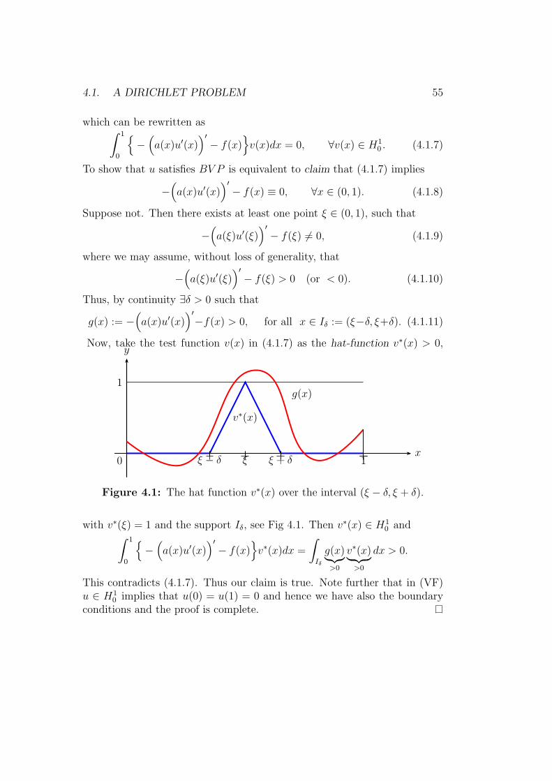
4.1. A DIRICHLET PROBLEM 55
which can be rewritten as∫ 1
0
−
(a(x)u′(x)
)′− f(x)
v(x)dx = 0, ∀v(x) ∈ H1
0 . (4.1.7)
To show that u satisfies BV P is equivalent to claim that (4.1.7) implies
−(a(x)u′(x)
)′− f(x) ≡ 0, ∀x ∈ (0, 1). (4.1.8)
Suppose not. Then there exists at least one point ξ ∈ (0, 1), such that
−(a(ξ)u′(ξ)
)′− f(ξ) 6= 0, (4.1.9)
where we may assume, without loss of generality, that
−(a(ξ)u′(ξ)
)′− f(ξ) > 0 (or < 0). (4.1.10)
Thus, by continuity ∃δ > 0 such that
g(x) := −(a(x)u′(x)
)′−f(x) > 0, for all x ∈ Iδ := (ξ−δ, ξ+δ). (4.1.11)
Now, take the test function v(x) in (4.1.7) as the hat-function v∗(x) > 0,
0
1
x
y
ξ − δ ξ ξ + δ
v∗(x)
1
g(x)
Figure 4.1: The hat function v∗(x) over the interval (ξ − δ, ξ + δ).
with v∗(ξ) = 1 and the support Iδ, see Fig 4.1. Then v∗(x) ∈ H10 and
∫ 1
0
−(a(x)u′(x)
)′− f(x)
v∗(x)dx =
∫
Iδ
g(x)︸︷︷︸>0
v∗(x)︸ ︷︷ ︸>0
dx > 0.
This contradicts (4.1.7). Thus our claim is true. Note further that in (VF)u ∈ H1
0 implies that u(0) = u(1) = 0 and hence we have also the boundaryconditions and the proof is complete.

56 CHAPTER 4. TWO-POINT BOUNDARY VALUE PROBLEMS
Corollary 4.1. (i) If f(x) is continuous and a(x) is continuously differ-entiable: f ∈ C(0, 1) and a ∈ C1(0, 1), then (BV P ), (V F ) have the samesolution.
(ii) If a(x) is discontinuous and f ∈ L2, then (BV P ) is not always well-defined but (V F ) has still a meaning. Therefore (V F ) covers a larger set ofdata than (BV P ).
(iii) More important: in (V F ), u ∈ C1(0, 1),while (BV P ) is formulated foru having two derivatives, i.e. u ∈ C2(0, 1).
The minimization problem (MP). For the problem (4.1.1), we may for-mulate yet another equivalent problem, viz:
Find u ∈ H10 such that F (u) ≤ F (w), ∀w ∈ H1
0 , where F (w) is the totalpotential energy of the displacement w(x), given by
(MP) F (w) =1
2
∫ 1
0
a(w′)2dx
Internal (elastic) energy
−∫ 1
0
fwdx.
Load potential
(4.1.12)
This means that the solution u minimizes the energy functional F (w). Belowwe show that the above minimization problem is equivalent to the variationalformulation (VF) and hence also to the boundary value problem (BVP).
Theorem 4.2. The following two properties are equivalent
a) u satisfies the variational formulation (VF)
b) u is the solution for the minimization problem (MP)
i.e.
∫ 1
0
au′v′dx =
∫ 1
0
fvdx, ∀v ∈ H10 ⇐⇒ F (u) ≤ F (w), ∀w ∈ H1
0 . (4.1.13)
Proof. (=⇒): First we show that the variational formulation (VF) impliesthe minimization problem (MP). To this end, for w ∈ H1
0 we let v = w − u,

4.1. A DIRICHLET PROBLEM 57
then, since H10 is a vector space and u ∈ H1
0 , hence v ∈ H10 and
F (w) = F (u+ v) =1
2
∫ 1
0
a((u+ v)′
)2
dx−∫ 1
0
f(u+ v)dx =
=1
2
∫ 1
0
2au′v′dx
︸ ︷︷ ︸(i)
+1
2
∫ 1
0
a(u′)2dx
︸ ︷︷ ︸(ii)
+1
2
∫ 1
0
a(v′)2dx
−∫ 1
0
fudx
︸ ︷︷ ︸(iii)
−∫ 1
0
fvdx.
︸ ︷︷ ︸(iv)
Now using (VF) we have (i) − (iv) = 0. Further by the definition of thefunctional F , (ii)− (iii) = F (u). Thus
F (w) = F (u) +1
2
∫ 1
0
a(x)(v′(x))2dx, (4.1.14)
and since a(x) > 0 we get F (w) ≥ F (u), thus we have proved ” =⇒ ” part.(⇐=): Next we show that the minimization problem (MP) implies the vari-ational formulation (VF). To this end, assume that F (u) ≤ F (w) ∀w ∈ H1
0 ,and for an arbitrary function v ∈ H1
0 , set gv(ε) = F (u+εv), then by (MP), g
(as a function of ε) has a minimum at ε = 0. In other words ∂∂εgv(ε)
∣∣∣ε=0
= 0.
We have that
gv(ε) = F (u+ εv) =1
2
∫ 1
0
a((u+ εv)′
)2
dx−∫ 1
0
f(u+ εv)dx =
=1
2
∫ 1
0
a(u′)2 + aε2(v′)2 + 2aεu′v′dx−∫ 1
0
fudx− ε
∫ 1
0
fvdx.
The derivative ∂gv∂ε
(ε), of g(ε, v) is
∂gv∂ε
(ε) =1
2
∫ 1
0
2aε(v′)2 + 2au′v′dx−∫ 1
0
fvdx, (4.1.15)
where ∂gv∂ε
∣∣∣(ε=0)
= 0, yields
∫ 1
0
au′v′dx−∫ 1
0
fvdx = 0, (4.1.16)
which is our desired variational formulation (VF). Hence, we conclude thatF (u) ≤ F (w), ∀w ∈ H1
0 =⇒ (VF), and the proof is complete.
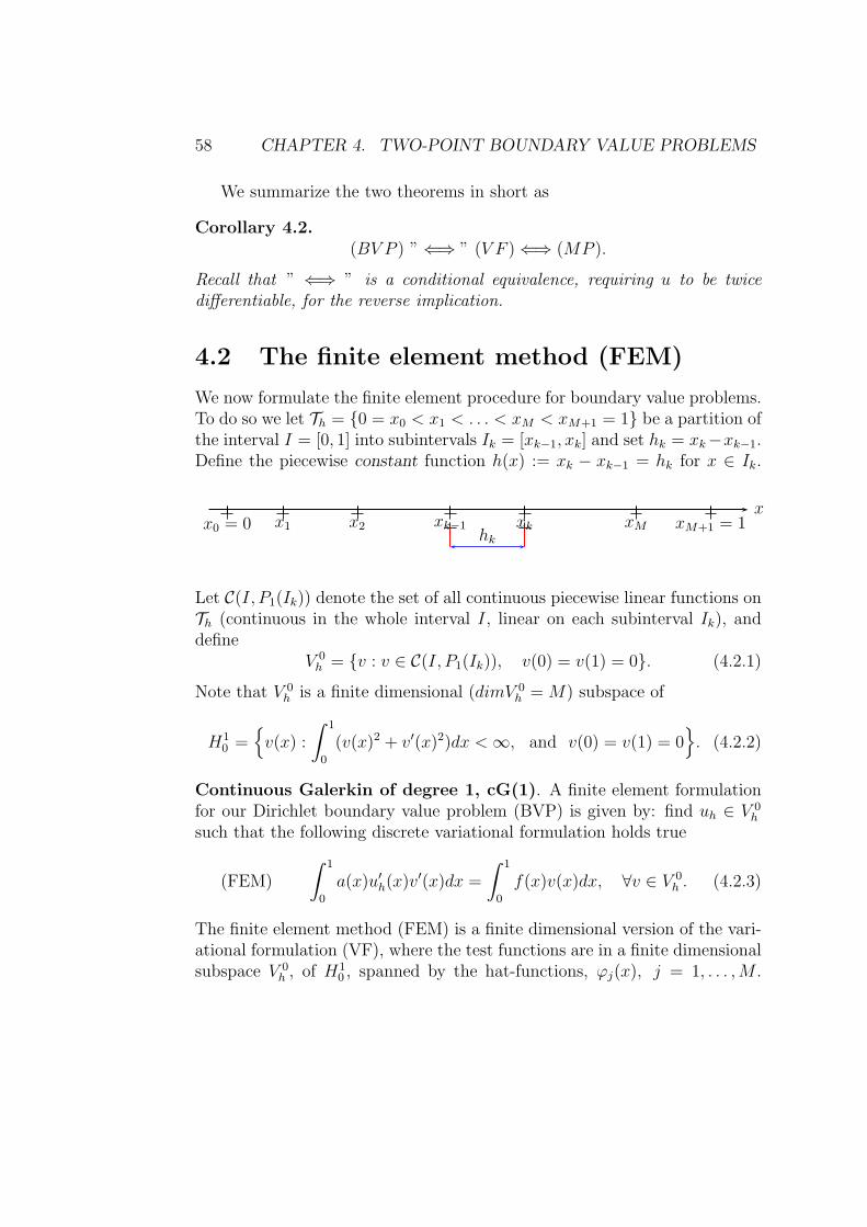
58 CHAPTER 4. TWO-POINT BOUNDARY VALUE PROBLEMS
We summarize the two theorems in short as
Corollary 4.2.(BV P ) ” ⇐⇒ ” (V F ) ⇐⇒ (MP ).
Recall that ” ⇐⇒ ” is a conditional equivalence, requiring u to be twicedifferentiable, for the reverse implication.
4.2 The finite element method (FEM)
We now formulate the finite element procedure for boundary value problems.To do so we let Th = 0 = x0 < x1 < . . . < xM < xM+1 = 1 be a partition ofthe interval I = [0, 1] into subintervals Ik = [xk−1, xk] and set hk = xk−xk−1.Define the piecewise constant function h(x) := xk − xk−1 = hk for x ∈ Ik.
x0 = 0 x1 x2 xk−1 xk xM xM+1 = 1x
hk
Let C(I, P1(Ik)) denote the set of all continuous piecewise linear functions onTh (continuous in the whole interval I, linear on each subinterval Ik), anddefine
V 0h = v : v ∈ C(I, P1(Ik)), v(0) = v(1) = 0. (4.2.1)
Note that V 0h is a finite dimensional (dimV 0
h =M) subspace of
H10 =
v(x) :
∫ 1
0
(v(x)2 + v′(x)2)dx <∞, and v(0) = v(1) = 0. (4.2.2)
Continuous Galerkin of degree 1, cG(1). A finite element formulationfor our Dirichlet boundary value problem (BVP) is given by: find uh ∈ V 0
h
such that the following discrete variational formulation holds true
(FEM)
∫ 1
0
a(x)u′h(x)v′(x)dx =
∫ 1
0
f(x)v(x)dx, ∀v ∈ V 0h . (4.2.3)
The finite element method (FEM) is a finite dimensional version of the vari-ational formulation (VF), where the test functions are in a finite dimensionalsubspace V 0
h , of H10 , spanned by the hat-functions, ϕj(x), j = 1, . . . ,M .
4.3. ERROR ESTIMATES IN THE ENERGY NORM 59
Thus, if in VF we restrict v to V 0h (rather that H1
0 ) and subtract FEM fromit, we get the Galerkin orthogonality:
∫ 1
0
a(x)(u′(x)− u′h(x))v′(x)dx = 0, ∀v ∈ V 0
h . (4.2.4)
Now the purpose is to estimate the error arising in approximating the solutionfor BV P by functions in V 0
h . To this approach we need some measuringenvironment for the error. We recall the definition of Lp-norms:
Lp-norm ‖v‖Lp=
(∫ 1
0
|v(x)|pdx)1/p
, 1 ≤ p <∞
L∞-norm ‖v‖L∞= max
x∈[0,1]|v(x)|,
and also introduce:
Weighted L2-norm ‖v‖a =(∫ 1
0
a(x)|v(x)|2dx)1/2
, a(x) > 0
Energy-norm ‖v‖E =(∫ 1
0
a(x)|v′(x)|2dx)1/2
,
Note that ‖v‖E = ‖v′‖a.
4.3 Error estimates in the energy norm
We shall study an a priori error estimate; where a certain norm of the error isestimated by some norm of the exact solution u. Here, the error analysis givesinformation about the size of the error, depending on the (unknown) exactsolution u, before any computational steps. An a posteriori error estimate;where the error is estimated by some norm of the residual of the approximatesolution is also included.
Below, first we shall prove a qualitative result which states that the finiteelement solution is the best approximate solution to the Dirichlet problemin the energy norm.
Theorem 4.3. Let u(x) be the solution to the Dirichlet boundary value prob-lem (4.1.1) and uh(x) its finite element approximation given by (4.2.3), then
‖u− uh‖E ≤ ‖u− v‖E, ∀v ∈ V 0h . (4.3.1)
This means that the finite element solution uh ∈ V 0h is the best approximation
of the solution u, in the energy norm, by functions in V 0h .
60 CHAPTER 4. TWO-POINT BOUNDARY VALUE PROBLEMS
Proof. We take an arbitrary v ∈ V 0h , then using the energy norm
‖u− uh‖2E =
∫ 1
0
a(x)(u′(x)− u′h(x))2 dx
=
∫ 1
0
a(x)(u′(x)− u′h(x))(u′(x)− v′(x) + v′(x)− u′h(x))dx
=
∫ 1
0
a(x)(u′(x)− u′h(x))(u′(x)− v′(x))dx
+
∫ 1
0
a(x)(u′(x)− u′h(x))(v′(x)− u′h(x)) dx.
(4.3.2)
Since v−uh ∈ V 0h , by Galerkin orthogonality (4.2.4), the last integral is zero.
Thus,
‖u− uh‖2E =
∫ 1
0
a(x)(u′(x)− u′h(x))(u′(x)− v′(x))dx
=
∫ 1
0
a(x)1
2 (u′(x)− u′h(x))a(x)1
2 (u′(x)− v′(x))dx
≤(∫ 1
0
a(x)(u′(x)− u′h(x))2dx
) 1
2(∫ 1
0
a(x)(u′(x)− v′(x))2dx) 1
2
= ‖u− uh‖E · ‖u− v‖E,(4.3.3)
where, in the last estimate, we used Cauchy-Schwarz inequality. Thus
‖u− uh‖E ≤ ‖u− v‖E, ∀v ∈ V 0h , (4.3.4)
and the proof is complete.
The next step is to show that there exists a function v(x) ∈ V 0h such that
‖u− v‖E is not too large. The function that we have in mind is πhu(x): thepiecewise linear interpolant of u(x), introduced in Chapter 3.
Theorem 4.4. [An a priori error estimate] Let u and uh be the solutionsof the Dirichlet problem (BVP) and the finite element problem (FEM), re-spectively. Then there exists an interpolation constant Ci, depending only ona(x), such that
‖u− uh‖E ≤ Ci‖hu′′‖a. (4.3.5)
4.3. ERROR ESTIMATES IN THE ENERGY NORM 61
Proof. Since πhu(x) ∈ V 0h , we may take v = πhu(x) in (4.3.1) and use, e.g.
the second estimate in the interpolation Theorem 3.3 (slightly generalized tothe weigthed norm ‖ · ‖a, see remark below) to get
‖u− uh‖E ≤ ‖u− πhu‖E = ‖u′ − (πhu)′‖a
≤ Ci‖hu′′‖a = Ci
(∫ 1
0
a(x)h2(x)u′′(x)2 dx)1/2
,(4.3.6)
which is the desired result and the proof is complete.
Remark 4.1. The interpolation theorem is not stated in the weighted norm.The a(x) dependence of the interpolation constant Ci can be shown as follows
‖u′ − (πhu)′‖a =
(∫ 1
0
a(x)(u′(x)− (πhu)′(x))2 dx
)1/2
≤(maxx∈[0,1]
a(x)1/2)· ‖u′ − (πhu)
′‖L2≤ ci
(maxx∈[0,1]
a(x)1/2)‖hu′′‖L2
= ci
(maxx∈[0,1]
a(x)1/2)(∫ 1
0
h(x)2u′′(x)2 dx)1/2
≤ ci(maxx∈[0,1] a(x)
1/2)
(minx∈[0,1] a(x)1/2)·(∫ 1
0
a(x)h(x)2u′′(x)2 dx)1/2
.
Thus
Ci = ci(maxx∈[0,1] a(x)
1/2)
(minx∈[0,1] a(x)1/2), (4.3.7)
where ci = c2 is the interpolation constant in the second estimate in Theorem3.3.
Remark 4.2. If the objective is to divide [0, 1] into a finite number of subin-tervals, then one can use the result of Theorem 4.4: to obtain an optimalpartition of [0, 1], where whenever a(x)u′′(x)2 gets large we compensate bymaking h(x) smaller. This, however, “requires that the exact solution u(x)is known” 1. Now we state the a posteriori error estimate, which instead ofthe unknown solution u(x), uses the residual of the computed solution uh(x).
Theorem 4.5 (An a posteriori error estimate). There is an interpolationconstant ci depending only on a(x) such that the error in the finite element
1Note that when a is a given constant then, −u′′(x) = (1/a)f(x) is known.

62 CHAPTER 4. TWO-POINT BOUNDARY VALUE PROBLEMS
approximation of the Dirichlet boundary value problem (4.1.10), satisfies
‖u− uh‖E ≤ ci
(∫ 1
0
1
a(x)h2(x)R2(uh(x))dx
)1/2
, (4.3.8)
where R(uh(x)) = f + (a(x)u′h(x))′ is the residual, and u(x)− uh(x) ∈ H1
0 .
Proof. By the definition of the energy norm we have
‖e(x)‖2E =
∫ 1
0
a(x)(e′(x))2dx =
∫ 1
0
a(x)(u′(x)− u′h(x))e′(x)dx
=
∫ 1
0
a(x)u′(x)e′(x)dx−∫ 1
0
a(x)u′h(x)e′(x)dx
(4.3.9)
Since e ∈ H10 the variational formulation (VF) gives that
∫ 1
0
a(x)u′(x)e′(x)dx =
∫ 1
0
f(x)e(x)dx. (4.3.10)
Hence, we can write
‖e(x)‖2E =
∫ 1
0
f(x)e(x)dx−∫ 1
0
a(x)u′h(x)e′(x)dx. (4.3.11)
Adding and subtracting the interpolant πhe(x) and its derivative (πhe)′(x)
to e and e′ in the integrands above yields
‖e(x)‖2E =
∫ 1
0
f(x)(e(x)− πhe(x))dx+
∫ 1
0
f(x)πhe(x)dx
︸ ︷︷ ︸(i)
−∫ 1
0
a(x)u′h(x)(e′(x)− (πhe)
′(x))dx−∫ 1
0
a(x)u′h(x)(πhe)′(x)dx
︸ ︷︷ ︸(ii)
.
Since uh(x) is the solution of the (FEM) given by (4.2.3) and πhe(x) ∈ V 0h
we have that −(ii) + (i) = 0. Hence
‖e(x)‖2E =
∫ 1
0
f(x)(e(x)− πhe(x))dx−∫ 1
0
a(x)u′h(x)(e′(x)− (πhe)
′(x))dx
=
∫ 1
0
f(x)(e(x)− πhe(x))dx−M+1∑
k=1
∫ xk
xk−1
a(x)u′h(x)(e′(x)− (πhe)
′(x))dx.
4.3. ERROR ESTIMATES IN THE ENERGY NORM 63
To continue we integrate by parts in the integrals in the summation above
−∫ xk
xk−1
a(x)u′h(x)(e′(x)− (πhe)
′(x))dx
= −[a(x)u′h(x)(e(x)− πhe(x))
]xk
xk−1
+
∫ xk
xk−1
(a(x)u′h(x))′(e(x)− πhe(x)) dx.
Now, using e(xk) = πhe(xk), k = 0, 1 . . . ,M + 1, where the xk:s are theinterpolation nodes, the boundary terms vanish and thus we end up with
−∫ xk
xk−1
a(x)u′h(x)(e′(x)− (πhe)
′(x))dx =
∫ xk
xk−1
(a(x)u′h(x))′(e(x)−πhe(x))dx.
Thus, summing over k, we have
−∫ 1
0
a(x)u′h(x)(e′(x)− (πhe(x))
′dx =
∫ 1
0
(a(x)u′h(x))′(e(x)− πhe(x))dx,
where (a(x)u′h(x))′ should be interpreted locally on each subinterval [xk−1, xk].
(Since u′h(x) in general is discontinuous, u′′h(x) does not exist globally on[0, 1].) Therefore
‖e(x)‖2E =
∫ 1
0
f(x)(e(x)− πhe(x))dx+
∫ 1
0
(a(x)u′h(x))′(e(x)− πhe(x))dx
=
∫ 1
0
f(x) + (a(x)u′h(x))′(e(x)− πhe(x))dx.
Now let R(uh(x)) = f(x) + (a(x)u′h(x))′, i.e. R(uh(x)) is the residual error,
which is a well-defined function except in the set xk, k = 1, . . . ,M ; where(a(xk)u
′h(xk))
′ is not defined. Then, using Cauchy-Schwarz’ inequality we getthe following estimate
‖e(x)‖2E =
∫ 1
0
R(uh(x))(e(x)− πhe(x))dx =
=
∫ 1
0
1√a(x)
h(x)R(uh(x)) ·√a(x)
(e(x)− πhe(x)
h(x)
)dx
≤(∫ 1
0
1
a(x)h2(x)R2(uh(x))dx
)1/2(∫ 1
0
a(x)(e(x)− πhe(x)
h(x)
)2
dx)1/2
.

64 CHAPTER 4. TWO-POINT BOUNDARY VALUE PROBLEMS
Further, by the definition of the weighted L2-norm we have,
∥∥∥e(x)− πhe(x)
h(x)
∥∥∥a=
(∫ 1
0
a(x)(e(x)− πhe(x)
h(x)
)2
dx)1/2
. (4.3.12)
To estimate (4.3.12) we can use the third interpolation estimate (in Theorem5.5) for e(x) in each subinterval and get
∥∥∥e(x)− πhe(x)
h(x)
∥∥∥a≤ Ci‖e′(x)‖a = Ci‖e(x)‖E, (4.3.13)
where Ci as before depends on a(x). Thus
‖e(x)‖2E ≤(∫ 1
0
1
a(x)h2(x)R2(uh(x))dx
)1/2
· Ci‖e(x)‖E, (4.3.14)
and the proof is complete.
Adaptivity
Below we briefly outline the adaptivity procedure based on the a posteriorierror estimate which uses the approximate solution and which can be usedfor mesh-refinements. Loosely speaking, the estimate (4.3.8) predicts localmesh refinement, i.e. indicates the regions (subintervals) which should besubdivided further. More specifically the idea is as follows: assume that oneseeks an error less than a given error tolerance TOL > 0:
‖e‖E ≤ TOL, e(x) := u(x)− uh(x). (4.3.15)
Then, one may use the following steps as a mesh refinement strategy:
(i) Make an initial partition of the interval
(ii) Compute the corresponding FEM solution uh(x) and residual R(uh(x)).
(iii) If ‖e‖E > TOL, refine the mesh in the places where1
a(x)R2(uh(x)) is
large and perform the steps (ii) and (iii) again.
4.4. FEM FOR CONVECTION–DIFFUSION–ABSORPTION BVPS 65
4.4 FEM for convection–diffusion–absorption
BVPs
We now return to the Galerkin approximation of a solution to boundaryvalue problems and give a framework for the cG(1) (continuous Galerkin ofdegree 1) finite element procedure leading to a linear system of equations ofthe form Aξ = b. More specifically, we shall extend the approach in Chapter2, for the stationary heat equation, to cases involving absorption and/orconvection terms. We also consider non-homogeneous Dirichlet boundaryconditions. We illustrate this procedure through the following two examples.
Example 4.1. Determine the coefficient matrix and load vector for the cG(1)finite element approximation of the boundary value problem
−u′′(x) + 4u(x) = 0, 0 < x < 1; u(0) = α 6= 0, u(1) = β 6= 0,
on a uniform partition Th of the interval [0, 1] into n+ 1 subintervals.Solution: The objective is to construct an approximate solution uh in a fi-nite dimensional space spanned by the piecewise linear basis functions (hat-functions) ϕj(x), j = 0, 1, . . . , n + 1 on the partition Th. This results in adiscrete problem represented by a linear system of equations Aξ = b, for theunknown ξ = cjnj=1, (c0 = α and cn+1 = β are given in boundary data.)The continuous solution is assumed to be in the Hilbert space
H1 =
w :
∫ 1
0
(w(x)2 + w′(x)2
)dx <∞
.
Since u(0) = α and u(1) = β are given, we need to take the trial functions in
V := w : w ∈ H1, w(0) = α, w(1) = β,
and the test functions in
V 0 := H10 = w : w ∈ H1, w(0) = w(1) = 0.
We multiply the PDE by a test function v ∈ V 0 and integrate over (0, 1).Integrating by parts we get
− u′(1)v(1) + u′(0)v(0) +
∫ 1
0
u′v′ dx+ 4
∫ 1
0
uv dx = 0 ⇐⇒
(V F ) : Find u ∈ V so that
∫ 1
0
u′v′ dx+ 4
∫ 1
0
uv dx = 0, ∀v ∈ V 0.
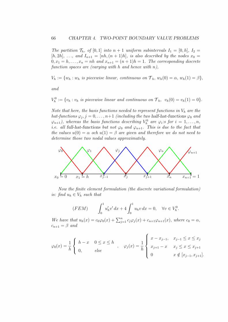
66 CHAPTER 4. TWO-POINT BOUNDARY VALUE PROBLEMS
The partition Th, of [0, 1] into n + 1 uniform subintervals I1 = [0, h], I2 =[h, 2h], . . ., and In+1 = [nh, (n + 1)h], is also described by the nodes x0 =0, x1 = h, . . . , xn = nh and xn+1 = (n+ 1)h = 1. The corresponding discretefunction spaces are (varying with h and hence with n),
Vh := wh : wh is piecewise linear, continuous on T h, wh(0) = α, wh(1) = β,
and
V 0h := vh : vh is piecewise linear and continuous on T h, vh(0) = vh(1) = 0.
Note that here, the basis functions needed to represent functions in Vh are thehat-functions ϕj, j = 0, . . . , n+1 (including the two half-hat-functions ϕ0 andϕn+1), whereas the basis functions describing V 0
h are ϕi:s for i = 1, . . . , n,i.e. all full-hat-functions but not ϕ0 and ϕn+1. This is due to the fact thatthe values u(0) = α och u(1) = β are given and therefore we do not need todetermine those two nodal values approximately.
ϕ0 ϕ1 ϕn+1ϕn
x0 = 0 x1 = h xn xn+1 = 1xj−1 xj xj+1
ϕj
Now the finite element formulation (the discrete variational formulation)is: find uh ∈ Vh such that
(FEM)
∫ 1
0
u′hv′ dx+ 4
∫ 1
0
uhv dx = 0, ∀v ∈ V 0h .
We have that uh(x) = c0ϕ0(x) +∑n
j=1 cjϕj(x) + cn+1ϕn+1(x), where c0 = α,cn+1 = β and
ϕ0(x) =1
h
h− x 0 ≤ x ≤ h
0, else, ϕj(x) =
1
h
x− xj−1, xj−1 ≤ x ≤ xj
xj+1 − x xj ≤ x ≤ xj+1
0 x /∈ [xj−1, xj+1].

4.4. FEM FOR CONVECTION–DIFFUSION–ABSORPTION BVPS 67
and
ϕn+1(x) =1
h
x− xn nh ≤ x ≤ (n+ 1)h
0, else..
Inserting uh into (FEM), and choosing v = ϕi(x), i = 1, . . . , n we get
n∑
j=1
(∫ 1
0
ϕ′j(x)ϕ
′i(x) dx+ 4
∫ 1
0
ϕj(x)ϕi(x) dx)cj
= −(∫ 1
0
ϕ′0(x)ϕ
′i(x) dx+ 4
∫ 1
0
ϕ0(x)ϕi(x) dx)c0
−(∫ 1
0
ϕ′n+1(x)ϕ
′i(x) dx+ 4
∫ 1
0
ϕn+1(x)ϕi(x) dx)cn+1.
In matrix form this corresponds to Aξ = b with A = S+4M , where S = Aunif
is the, previously computed, stiffness matrix:
S =1
h
2 −1 0 0 . . . 0
−1 2 −1 0 . . . 0
0 −1 2 −1 . . . 0
. . . . . . . . . . . . . . . . . .
0 . . . . . . −1 2 −1
0 . . . . . . . . . −1 2
, (4.4.1)
and M is the mass-matrix given by
M =
∫ 1
0ϕ1ϕ1
∫ 1
0ϕ2ϕ1 . . .
∫ 1
0ϕnϕ1
∫ 1
0ϕ1ϕ2
∫ 1
0ϕ2ϕ2 . . .
∫ 1
0ϕnϕ2
. . . . . . . . . . . .∫ 1
0ϕ1ϕn
∫ 1
0ϕ2ϕn . . .
∫ 1
0ϕnϕn
. (4.4.2)
Note the index locations in the matrices S and M :
sij =
∫ 1
0
ϕ′j(x)ϕ
′i(x) dx, mij =
∫ 1
0
ϕj(x)ϕi(x) dx.

68 CHAPTER 4. TWO-POINT BOUNDARY VALUE PROBLEMS
This, however, does not make any difference in the current example, since,as seen, both S and M are symmetric. To compute the entries of M , wefollow the same procedure as in Chapter 2, and notice that, as S, also M issymmetric and its elements mij are
mij = mji =
∫ 1
0ϕiϕj dx = 0, ∀i, j with |i− j| > 1
∫ 1
0ϕ2j(x) dx, for i = j
∫ 1
0ϕj(x)ϕj+1(x), for i = j + 1.
(4.4.3)
1
x
y
xj−1 xj xj+1 xj+2
ϕj−1 ϕj ϕj+1 ϕj+2
Figure 4.2: ϕj and ϕj+1.
The diagonal elements are
mjj =
∫ 1
0
ϕj(x)2 dx =
1
h2
(∫ xj
xj−1
(x− xj−1)2 dx+
∫ xj+1
xj
(xj+1 − x)2)
=1
h2
[(x− xj−1)3
3
]xj
xj−1
− 1
h2
[(xj+1 − x)3
3
]xj+1
xj
=1
h2· h
3
3+
1
h2· h
3
3=
2
3h, j = 1, . . . , n,
(4.4.4)
4.4. FEM FOR CONVECTION–DIFFUSION–ABSORPTION BVPS 69
and the two super- and sub-diagonals can be computed as
mj,j+1 = mj+1,j =
∫ 1
0
ϕjϕj+1 dx =1
h2
∫ xj+1
xj
(xj+1 − x)(x− xj) = [PI]
=1
h2
[(xj+1 − x)
(x− xj)2
2
]xj+1
xj
− 1
h2
∫ xj+1
xj
−(x− xj)2
2dx
=1
h2
[(x− xj)3
6
]xj+1
xj
=1
6h, j = 1, . . . , n− 1.
Thus the mass matrix in this case is
M = h
23
16
0 0 . . . 0
16
23
16
0 . . . 0
0 16
23
16
. . . 0
. . . . . . . . . . . . . . . . . .
0 . . . . . . 16
23
16
0 . . . . . . . . . 16
23
=h
6
4 1 0 0 . . . 0
1 4 1 0 . . . 0
0 1 4 1 . . . 0
. . . . . . . . . . . . . . . . . .
0 . . . . . . 1 4 1
0 . . . . . . . . . 1 4
.
Hence, for i, j = 1, . . . , n, the coefficient matrix A = S + 4M is given by
[A]ij =
∫ 1
0
ϕ′iϕ
′j dx+ 4
∫ 1
0
ϕiϕj(x) dx =
2h+ 8h
3, i = j,
− 1h+ 2h
3, |i− j| = 1,
0 else.
Finally, with c0 = α och cn+1 = β, we get the load vector viz,
b1 = −(−1
h+
2h
3)c0 = α(
1
h− 2h
3),
b2 = . . . = bn−1 = 0,
bn = −(−1
h+
2h
3)cn+1 = β(
1
h− 2h
3).
Now, for each particular choice of h (i.e. n), α and β we may solve Aξ =b to obtain the nodal values of the approximate solution uh at the innernodes xj, j = 1, . . . , n. That is: ξ = (c1, . . . , cn)
T := (uh(x1), . . . , uh(xn))T .
Connecting the points (xj, uh(xj)), j = 0, . . . , n+1 by straight lines we obtainthe desired continuous piecewise linear approximation of the solution.

70 CHAPTER 4. TWO-POINT BOUNDARY VALUE PROBLEMS
Remark 4.3. An easier way to compute the above integrals mj,j+1 (as wellas mjj) is through Simpson’s rule, which is exact for polynomials of degree≤ 2. Since ϕj(x)ϕj+1(x) = 0 at x = xj and x = xj+1, we need to evaluateonly the midterm of the Simpson’s formula, i.e.∫ 1
0
ϕjϕj+1 dx = 4h
6ϕj
(xj + xj+1
2
)· ϕj+1
(xj + xj+1
2
)· = 4 · h
6· 12· 12=h
6.
For a uniform partition one may use ϕ0 = 1− x/h and ϕ1 = x/h on (0, h) :
∫ 1
0
ϕ0ϕ1 dx =
∫ h
0
(1− x
h)x
hdx =
[(1− x
h)x2
2h
]h0−
∫ h
0
(−1)
h· x
2
2hdx =
h
6.
Example 4.2. Below we consider a convection-diffusion problem:
−εu′′(x) + pu′(x) = r, 0 < x < 1; u(0) = 0, u′(1) = β 6= 0,
where ε and p are positive real numbers and r ∈ R. Here −εu′′ is the diffusionterm, pu′ corresponds to convection, and r is a given (here for simplicity aconstant) source (r > 0) or sink (r < 0). We would like to answer the samequestion as in the previous example. This time with c0 = u(0) = 0. Then,the test function at x = 0; ϕ0 will not be necessary. But since u(1) is notgiven, we shall need the test function at x = 1: ϕn+1. The function space forthe continuous solution: the trial function space, and the test function spaceare both the same:
V :=
w :
∫ 1
0
(w(x)2 + w′(x)2
)dx <∞, and w(0) = 0
.
We multiply the PDE by a test function v ∈ V and integrate over (0, 1).Then, integration by parts yields
−εu′(1)v(1) + εu′(0)v(0) + ε
∫ 1
0
u′v′dx+ p
∫ 1
0
u′vdx = r
∫ 1
0
v dx.
Hence, we end up with the variational formulation: find u ∈ V such that
(VF) ε
∫ 1
0
u′v′ dx+ p
∫ 1
0
u′v dx = r
∫ 1
0
v dx+ εβv(1), ∀v ∈ V.
The corresponding discrete test and trial function space is
V 0h := wh : wh is piecewise linear and continuous on T h, and wh(0) = 0.

4.4. FEM FOR CONVECTION–DIFFUSION–ABSORPTION BVPS 71
ϕ0 ϕ2 ϕn+1ϕn
x0 = 0 x1 = h xn xn+1 = 1xj−1 xj xj+1
ϕj
Thus, the basis functions for V 0h are the hat-functions ϕj, j = 1, . . . , n + 1
(including the half-hat-function ϕn+1), and hence dim(V 0h ) = n+ 1.
Now the finite element formulation reads as follows: find uh ∈ V 0h such that
(FEM) ε
∫ 1
0
u′hv′ dx+ p
∫ 1
0
u′hv dx = r
∫ 1
0
v dx+ εβv(1), ∀v ∈ V 0h .
Inserting the ansatz uh(x) =∑n+1
j=1 ξjϕj(x) into (FEM), and choosing v =ϕi(x), i = 1, . . . , n+ 1, we get
n+1∑
j=1
(ε
∫ 1
0
ϕ′j(x)ϕ
′i(x) dx+ p
∫ 1
0
ϕ′j(x)ϕi(x) dx
)ξj = r
∫ 1
0
ϕi(x) dx+ εβϕi(1),
In matrix form this corresponds to the linear system of equations Aξ = b withA = ε S + pC, where S is computed as Aunif and is the (n + 1) × (n + 1)-
stiffness matrix with its last diagonal element sn+1,n+1 =∫ 1
0ϕ′n+1ϕ
′n+1 dx =
1/h, and C is the convection matrix with the elements
cij =
∫ 1
0
ϕ′j(x)ϕi(x) dx.
Hence we have, evidently,
S =1
h
2 −1 0 0 . . . 0
−1 2 −1 0 . . . 0
0 −1 2 −1 . . . 0
. . . . . . . . . . . . . . . . . .
0 . . . . . . −1 2 −1
0 . . . . . . . . . −1 1
.
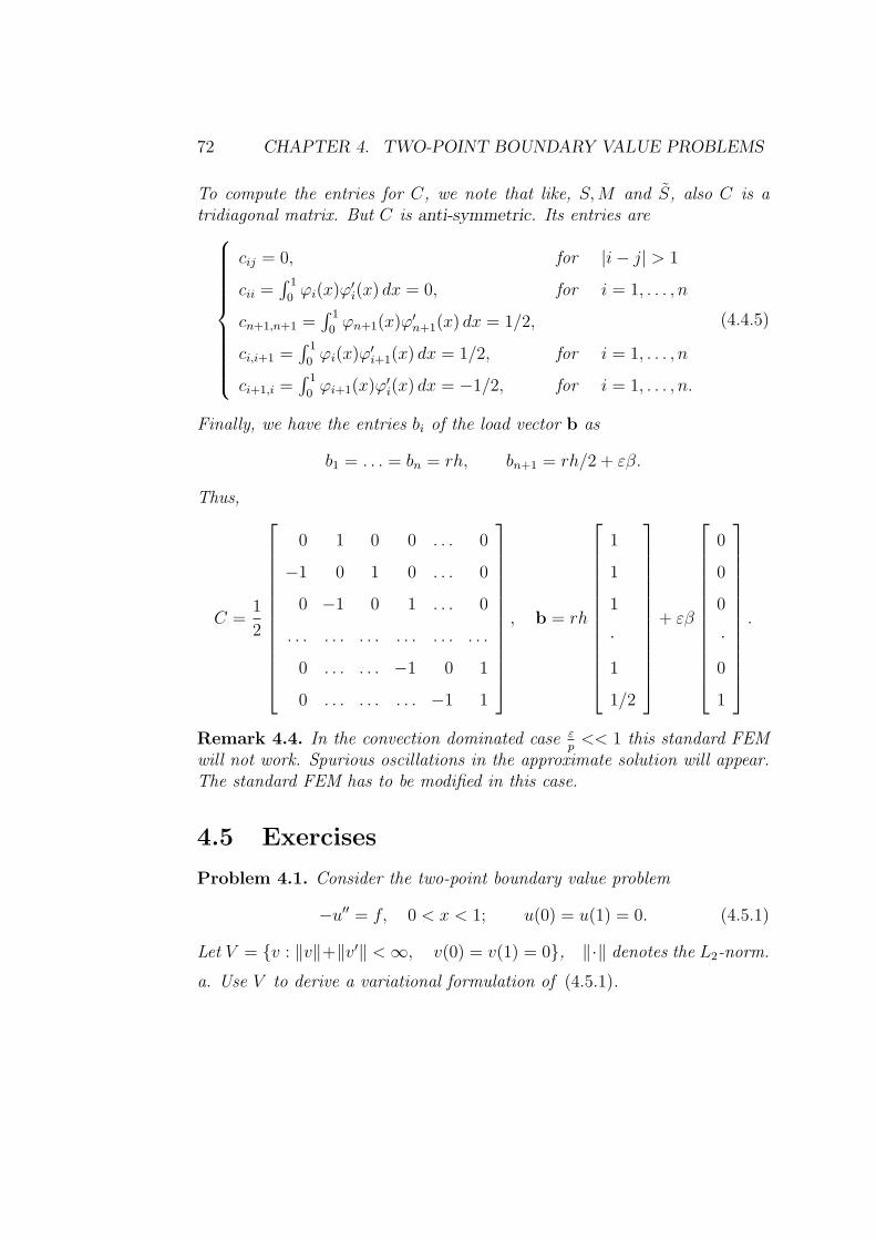
72 CHAPTER 4. TWO-POINT BOUNDARY VALUE PROBLEMS
To compute the entries for C, we note that like, S,M and S, also C is atridiagonal matrix. But C is anti-symmetric. Its entries are
cij = 0, for |i− j| > 1
cii =∫ 1
0ϕi(x)ϕ
′i(x) dx = 0, for i = 1, . . . , n
cn+1,n+1 =∫ 1
0ϕn+1(x)ϕ
′n+1(x) dx = 1/2,
ci,i+1 =∫ 1
0ϕi(x)ϕ
′i+1(x) dx = 1/2, for i = 1, . . . , n
ci+1,i =∫ 1
0ϕi+1(x)ϕ
′i(x) dx = −1/2, for i = 1, . . . , n.
(4.4.5)
Finally, we have the entries bi of the load vector b as
b1 = . . . = bn = rh, bn+1 = rh/2 + εβ.
Thus,
C =1
2
0 1 0 0 . . . 0
−1 0 1 0 . . . 0
0 −1 0 1 . . . 0
. . . . . . . . . . . . . . . . . .
0 . . . . . . −1 0 1
0 . . . . . . . . . −1 1
, b = rh
1
1
1
·1
1/2
+ εβ
0
0
0
·0
1
.
Remark 4.4. In the convection dominated case εp<< 1 this standard FEM
will not work. Spurious oscillations in the approximate solution will appear.The standard FEM has to be modified in this case.
4.5 Exercises
Problem 4.1. Consider the two-point boundary value problem
−u′′ = f, 0 < x < 1; u(0) = u(1) = 0. (4.5.1)
Let V = v : ‖v‖+‖v′‖ <∞, v(0) = v(1) = 0, ‖·‖ denotes the L2-norm.
a. Use V to derive a variational formulation of (4.5.1).

4.5. EXERCISES 73
b. Discuss why V is valid as a vector space of test functions.
c. Classify which of the following functions are admissible test functions
sin πx, x2, x ln x, ex − 1, x(1− x).
Problem 4.2. Assume that u(0) = u(1) = 0, and that u satisfies∫ 1
0
u′v′ dx =
∫ 1
0
fv dx,
for all v ∈ V = v : ‖v‖+ ‖v′‖ <∞, v(0) = v(1) = 0.a. Show that u minimizes the functional
F (v) =1
2
∫ 1
0
(v′)2 dx−∫ 1
0
fv dx. (4.5.2)
Hint: F (v) = F (u+ w) = F (u) + . . . ≥ F (u).
b. Prove that the above minimization problem is equivalent to
−u′′ = f, 0 < x < 1; u(0) = u(1) = 0.
Problem 4.3. Consider the two-point boundary value problem
−u′′ = 1, 0 < x < 1; u(0) = u(1) = 0. (4.5.3)
Let Th : xj =j4, j = 0, 1, . . . , 4, denote a partition of the interval 0 < x < 1
into four subintervals of equal length h = 1/4 and let Vh be the correspondingspace of continuous piecewise linear functions vanishing at x = 0 and x = 1.
a. Compute a finite element approximation U ∈ Vh to (4.5.3).
b. Prove that U ∈ Vh is unique.
Problem 4.4. Consider once again the two-point boundary value problem
−u′′ = f, 0 < x < 1; u(0) = u(1) = 0.
a. Prove that the finite element approximation U ∈ Vh to u satisfies
‖(u− U)′‖ ≤ ‖(u− v)′‖, for all v ∈ Vh.
b. Use this result and interpolation estimate to deduce that
‖(u− U)′‖ ≤ C‖hu′′‖, (4.5.4)
where C depends on the interpolation constant.
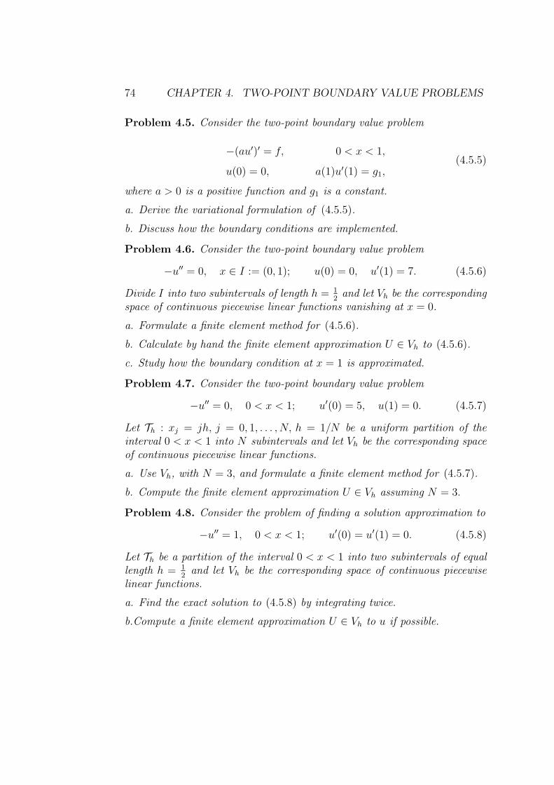
74 CHAPTER 4. TWO-POINT BOUNDARY VALUE PROBLEMS
Problem 4.5. Consider the two-point boundary value problem
−(au′)′ = f, 0 < x < 1,
u(0) = 0, a(1)u′(1) = g1,(4.5.5)
where a > 0 is a positive function and g1 is a constant.
a. Derive the variational formulation of (4.5.5).
b. Discuss how the boundary conditions are implemented.
Problem 4.6. Consider the two-point boundary value problem
−u′′ = 0, x ∈ I := (0, 1); u(0) = 0, u′(1) = 7. (4.5.6)
Divide I into two subintervals of length h = 12and let Vh be the corresponding
space of continuous piecewise linear functions vanishing at x = 0.
a. Formulate a finite element method for (4.5.6).
b. Calculate by hand the finite element approximation U ∈ Vh to (4.5.6).
c. Study how the boundary condition at x = 1 is approximated.
Problem 4.7. Consider the two-point boundary value problem
−u′′ = 0, 0 < x < 1; u′(0) = 5, u(1) = 0. (4.5.7)
Let Th : xj = jh, j = 0, 1, . . . , N, h = 1/N be a uniform partition of theinterval 0 < x < 1 into N subintervals and let Vh be the corresponding spaceof continuous piecewise linear functions.
a. Use Vh, with N = 3, and formulate a finite element method for (4.5.7).
b. Compute the finite element approximation U ∈ Vh assuming N = 3.
Problem 4.8. Consider the problem of finding a solution approximation to
−u′′ = 1, 0 < x < 1; u′(0) = u′(1) = 0. (4.5.8)
Let Th be a partition of the interval 0 < x < 1 into two subintervals of equallength h = 1
2and let Vh be the corresponding space of continuous piecewise
linear functions.
a. Find the exact solution to (4.5.8) by integrating twice.
b.Compute a finite element approximation U ∈ Vh to u if possible.
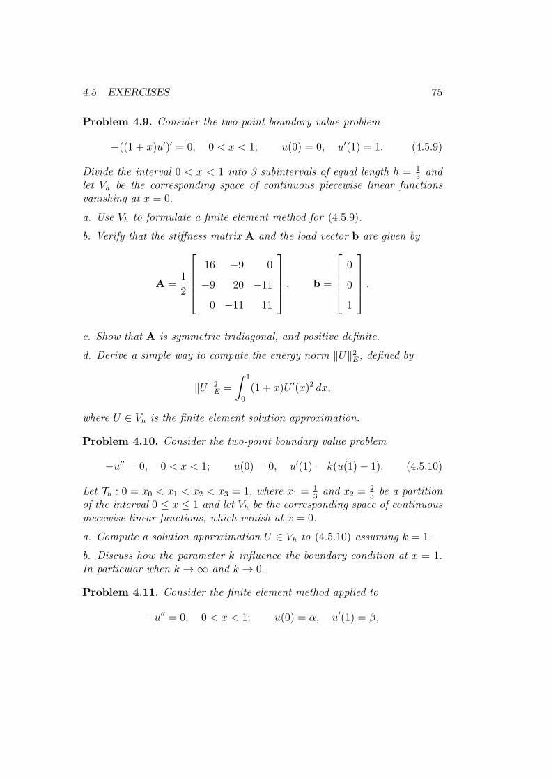
4.5. EXERCISES 75
Problem 4.9. Consider the two-point boundary value problem
−((1 + x)u′)′ = 0, 0 < x < 1; u(0) = 0, u′(1) = 1. (4.5.9)
Divide the interval 0 < x < 1 into 3 subintervals of equal length h = 13and
let Vh be the corresponding space of continuous piecewise linear functionsvanishing at x = 0.
a. Use Vh to formulate a finite element method for (4.5.9).
b. Verify that the stiffness matrix A and the load vector b are given by
A =1
2
16 −9 0
−9 20 −11
0 −11 11
, b =
0
0
1
.
c. Show that A is symmetric tridiagonal, and positive definite.
d. Derive a simple way to compute the energy norm ‖U‖2E, defined by
‖U‖2E =
∫ 1
0
(1 + x)U ′(x)2 dx,
where U ∈ Vh is the finite element solution approximation.
Problem 4.10. Consider the two-point boundary value problem
−u′′ = 0, 0 < x < 1; u(0) = 0, u′(1) = k(u(1)− 1). (4.5.10)
Let Th : 0 = x0 < x1 < x2 < x3 = 1, where x1 =13and x2 =
23be a partition
of the interval 0 ≤ x ≤ 1 and let Vh be the corresponding space of continuouspiecewise linear functions, which vanish at x = 0.
a. Compute a solution approximation U ∈ Vh to (4.5.10) assuming k = 1.
b. Discuss how the parameter k influence the boundary condition at x = 1.In particular when k → ∞ and k → 0.
Problem 4.11. Consider the finite element method applied to
−u′′ = 0, 0 < x < 1; u(0) = α, u′(1) = β,
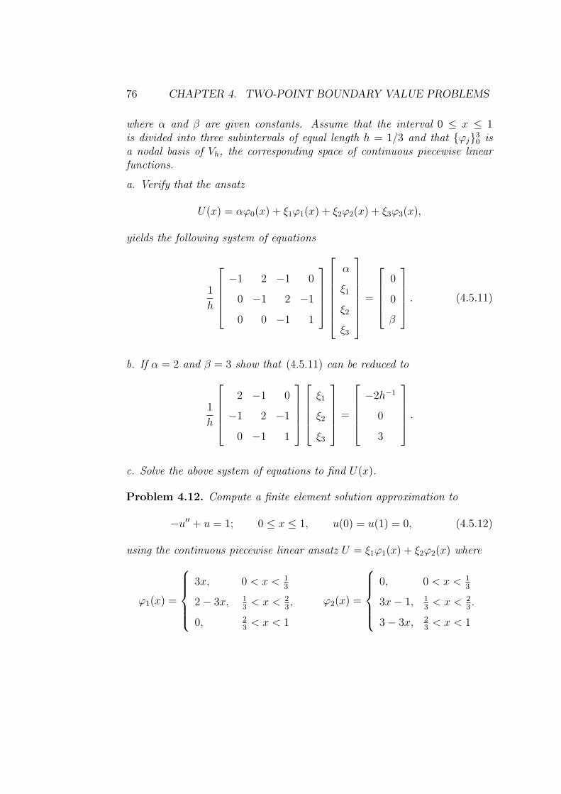
76 CHAPTER 4. TWO-POINT BOUNDARY VALUE PROBLEMS
where α and β are given constants. Assume that the interval 0 ≤ x ≤ 1is divided into three subintervals of equal length h = 1/3 and that ϕj30 isa nodal basis of Vh, the corresponding space of continuous piecewise linearfunctions.
a. Verify that the ansatz
U(x) = αϕ0(x) + ξ1ϕ1(x) + ξ2ϕ2(x) + ξ3ϕ3(x),
yields the following system of equations
1
h
−1 2 −1 0
0 −1 2 −1
0 0 −1 1
α
ξ1
ξ2
ξ3
=
0
0
β
. (4.5.11)
b. If α = 2 and β = 3 show that (4.5.11) can be reduced to
1
h
2 −1 0
−1 2 −1
0 −1 1
ξ1
ξ2
ξ3
=
−2h−1
0
3
.
c. Solve the above system of equations to find U(x).
Problem 4.12. Compute a finite element solution approximation to
−u′′ + u = 1; 0 ≤ x ≤ 1, u(0) = u(1) = 0, (4.5.12)
using the continuous piecewise linear ansatz U = ξ1ϕ1(x) + ξ2ϕ2(x) where
ϕ1(x) =
3x, 0 < x < 13
2− 3x, 13< x < 2
3,
0, 23< x < 1
ϕ2(x) =
0, 0 < x < 13
3x− 1, 13< x < 2
3.
3− 3x, 23< x < 1
4.5. EXERCISES 77
Problem 4.13. Consider the following eigenvalue problem
−au′′ + bu = 0; 0 ≤ x ≤ 1, u(0) = u′(1) = 0, (4.5.13)
where a, b > 0 are constants. Let Th : 0 = x0 < x1 < . . . < xN = 1,be a non-uniform partition of the interval 0 ≤ x ≤ 1 into N intervals oflength hi = xi − xi−1, i = 1, 2, . . . , N and let Vh be the corresponding spaceof continuous piecewise linear functions. Compute the stiffness and massmatrices.
Problem 4.14. Show that the FEM with the mesh size h for the problem:
−u′′ = 1 0 < x < 1
u(0) = 1 u′(1) = 0,(4.5.14)
with
U(x) = 7ϕ0(x) + U1ϕ1(x) + . . .+ Umϕm(x). (4.5.15)
leads to the linear system of equations: A · U = b, where
A =1
h
−1 2 −1 0
0 −1 2 −1 . . .
. . . . . . . . . . . .
0 . . . 0 . . .
,
m× (m+ 1)
U =
7
U1
. . .
Um
,
(m+ 1)× 1
b =
h
. . .
h
h/2
,
m× 1
. which is reduced to AU = b, with
A =1
h
2 −1 0 . . . 0
−1 2 −1 0 . . .
. . . . . . . . . . . . . . .
. . . 0 −1 2 −1
0 0 0 −1 2
, U =
U1
U2
. . .
Um
, b =
h+ 7h
h
. . .
h
h/2
.

78 CHAPTER 4. TWO-POINT BOUNDARY VALUE PROBLEMS
Problem 4.15. Prove an a priori error estimate for the cG(1) finite elementmethod for the problem
−u′′ + αu = f, in I = (0, 1), u(0) = u(1) = 0,
where the coefficient α = α(x) is a bounded positive function on I, (0 ≤α(x) ≤ K, x ∈ I).
Problem 4.16. a) Formulate a cG(1) method for the problem
(a(x)u′(x))′ = 0, 0 < x < 1,
a(0)u′(0) = u0, u(1) = 0.
and give an a priori error estimate.
b) Let u0 = 3 and compute the approximate solution in a) for a uniformpartition of I = [0, 1] into 4 intervals and
a(x) =
1/4, x < 1/2,
1/2, x > 1/2.
c) Show that, with these special choices, the computed solution is equal to theexact one, i.e. the error is equal to 0.
Problem 4.17. Prove an a priori error estimate for the finite elementmethod for the problem
−u′′(x) + u′(x) = f(x), 0 < x < 1, u(0) = u(1) = 0.
Problem 4.18. (a) Prove an a priori error estimate for the cG(1) approxi-mation of the boundary value problem
−u′′ + cu′ + u = f in I = (0, 1), u(0) = u(1) = 0,
where c ≥ 0 is constant.
(b) For which value of c is the a priori error estimate optimal?

4.5. EXERCISES 79
Problem 4.19. Let U be the piecewise linear finite element approximationfor
−u′′(x) + 2xu′(x) + 2u(x) = f(x), x ∈ (0, 1), u(0) = u(1) = 0,
in a partition Th of the interval [0, 1]. Set e = u−U and derive a priori errorestimates in the energy-norm:
||e||2E = ||e′||2 + ||e||2, where ||w||2 =∫ 1
0
w(x)2 dx.

80 CHAPTER 4. TWO-POINT BOUNDARY VALUE PROBLEMS
Chapter 5
Scalar Initial Value Problems
This chapter is devoted to numerical methods for time discretizations. Here, weshall consider problems depending on the time variable, only. The approximationtechniques developed in this chapter, combined with those of the previous chap-ter for boundary value problems, can be used for the numerical study of initialboundary value problems; such as, e.g. the heat and wave equations.
As a model problem we shall consider the classical example of populationdynamics described by the following ordinary differential equation (ODE)
(DE)
(IV)
u(t) + a(t)u(t) = f(t), 0 < t ≤ T,
u(0) = u0,(5.0.1)
where f(t) is the source term and u(t) =du
dt. The coefficient a(t) is a bounded
function. If a(t) ≥ 0 the problem (5.0.1) is called parabolic, while a(t) ≥ α > 0yields a dissipative problem, in the sense that, with increasing t, perturbationsof solutions to (5.0.1), e.g. introduced by numerical discretization, will decay.In general, in numerical approximations for (5.0.1), the error accumulates whenadvancing in time, i.e. the error of previous time steps adds up to the error ofthe present time step. The different types of error accumulation/perturbationgrowth are referred to as stability properties of the initial value problem.
81

82 CHAPTER 5. SCALAR INITIAL VALUE PROBLEMS
5.1 Solution formula and stability
Theorem 5.1. The solution of the problem (5.0.1) is given by
u(t) = u0 · e−A(t) +
∫ t
0
e−(A(t)−A(s))f(s)ds, (5.1.1)
where A(t) =∫ t
0a(s)ds and eA(t) is the integrating factor.
Proof. Multiplying the (DE) by the integrating factor eA(t) we have
u(t)eA(t) + A(t)eA(t)u(t) = eA(t)f(t), (5.1.2)
where we used that a(t) = A(t). Equation (5.1.2) can be rewritten as
d
dt
(u(t)eA(t)
)= eA(t)f(t).
We denote the variable by s and integrate from 0 to t to get∫ t
0
d
ds
(u(s)eA(s)
)ds =
∫ t
0
eA(s)f(s)ds,
i.e.
u(t)eA(t) − u(0)eA(0) =
∫ t
0
eA(s)f(s)ds.
Now since A(0) = 0 and u(0) = u0 we get the desired result
u(t) = u0e−A(t) +
∫ t
0
e−(A(t)−A(s))f(s)ds. (5.1.3)
This representation of u is known as the Variation of constants formula.
Theorem 5.2 (Stability estimates). Using the solution formula, we can de-rive the following stability estimates:
(i) If a(t) ≥ α > 0, then |u(t)| ≤ e−αt|u0|+1
α(1− e−αt) max
0≤s≤t|f(s)|,
(ii) If a(t) ≥ 0 (i.e. α = 0; the parabolic case), then
|u(t)| ≤ |u0|+∫ t
0
|f(s)|ds or |u(t)| ≤ |u0|+ ‖f‖L1(0,t). (5.1.4)

5.2. FINITE DIFFERENCE METHODS 83
Proof. (i) For a(t) ≥ α > 0 we have that A(t) =
∫ t
0
a(s)ds is an increasing
function of t, A(t) ≥ αt and
A(t)− A(s) =
∫ t
0
a(r) dr −∫ s
0
a(r) dr =
∫ t
s
a(r) dr ≥ α(t− s). (5.1.5)
Thus e−A(t) ≤ e−αt and e−(A(t)−A(s)) ≤ e−α(t−s). Hence, using (5.1.3) we get
|u(t)| ≤ |u0|e−αt +
∫ t
0
e−α(t−s)|f(s)|ds, (5.1.6)
which yields
|u(t)| ≤ e−αt|u0|+ max0≤s≤t
|f(s)|[ 1αe−α(t−s)
]s=t
s=0, i.e.
|u(t)| ≤ e−αt|u0|+1
α(1− e−αt) max
0≤s≤t|f(s)|.
(ii) Let α = 0 in (5.1.6) (which is true also in this case: for α = 0), then
|u(t)| ≤ |u0|+∫ t
0
|f(s)|ds, and the proof is complete.
Remark 5.1. (i) expresses that the effect of the initial data u0 decays expo-nentially with time, and that the effect of the source term f on the right handside does not depend on the length of the time interval, only on the maximumvalue of f , and on the value of α. In case (ii), the influence of u0 remainsbounded in time, and the integral of f indicates an accumulation in time.
5.2 Finite difference methods
Let us first continue as in Example 2.1 and give the other two, very common,finite difference approaches, for numerical solution of (5.0.1): Let
Tk := 0 = x0 < x1 <, . . . < xN−1 < xN = T,
be a partition of the time interval [0, T ] into the subintervals Ik := [xk−1, xk], k =1, . . . N as in the Example 2.1:

84 CHAPTER 5. SCALAR INITIAL VALUE PROBLEMS
t0 = 0 t1 t2 t3 tN = T
Example 5.1. Now we discretize the IVP (5.0.1), for a(t) being positiveconstant, with the backward Euler method, on the partition Tk, approximat-ing the derivative u(t) by a backward-difference quotient at each subinterval
Ik = (tk−1, tk] by u(t) ≈ u(tk)−u(tk−1)
tk−tk−1. Then an approximation of (5.0.1), with
f(t) ≡ 0 is given by
u(tk)− u(tk−1)
tk − tk−1
= −a · u(tk), k = 1, . . . , N, and u(0) = u0. (5.2.1)
(Note that in forward Euler, we would have −au(tk−1) on the right hand sideof (5.2.1)). Letting ∆tk = tk − tk−1, (5.2.1) yields
(1 + a∆tk)u(tk) = u(tk−1). (5.2.2)
Starting with k = 1 and the data u(0) = u0, the solution u(tk) would, itera-tively, be computed at the subsequent points: t1, t2, . . . , tN = T .For a uniform partition, where all subintervals have the same length ∆t, andsince for a > 0, 1 + a∆t > 0 ( 6= 0), (5.2.2) can be written as
u(tk) = (1 + a∆t)−1u(tk−1), k = 1, 2, . . . , N. (5.2.3)
Iterating we get the Backward or Implicit Euler method for (5.0.1):
u(tk) = (1 + a∆t)−1u(tk−1) = (1 + a∆t)−2u(tk−2) = . . . = (1 + a∆t)−ku0.
Remark 5.2. Note that, for the problem (5.0.1), with f(t) ≡ 0, in theExample 2.1 we just replace λ with −a, and get the forward (explicit) Eulermethod:
u(tk) = (1− a∆t)ku0. (5.2.4)
Example 5.2. Now we introduce the Crank-Nicolson method for the finitedifference approximation of (5.0.1). Here, first we integrate the equation(5.0.1) over Ik = [tk−1, tk] to get
u(tk)− u(tk−1) + a
∫ tk
tk−1
u(t) dt =
∫ tk
tk−1
f(t) dt. (5.2.5)
5.2. FINITE DIFFERENCE METHODS 85
Then, approximate the integral term by the simple trapezoidal rule we get
u(tk)− u(tk−1) + a∆tk2
(u(tk) + u(tk−1)) =
∫ tk
tk−1
f(t) dt. (5.2.6)
Rearranging the terms yields
(1 + a
∆tk2
)u(tk) =
(1− a
∆tk2
)u(tk−1) +
∫ tk
tk−1
f(t) dt.
Or, equivalently,
u(tk) =1− a∆tk/2
1 + a∆tk/2u(tk−1) +
1
1 + a∆tk/2
∫ tk
tk−1
f(t) dt.
Let us assume a zero source term (f = 0), and uniform partition, i.e. ∆tk =∆t for k = 1, 2, . . . , N , then we have the following Crank-Nicolson method:
u(tk) =(1− a∆t/2
1 + a∆t/2
)k
u0. (5.2.7)
Example 5.3. Consider the initial value problem:
u(t) + au(t) = 0, t > 0, u(0) = 1.
a) Let a = 40, and the time step k = 0.1. Draw the graph of Un :=U(nk), k = 1, 2, . . . , approximating u using (i) explicit (forward) Euler, (ii)implicit (Backward) Euler, and (iii) Crank-Nicolson methods.
b) Consider the case a = i, (i2 = −1), having the complex solution u(t) = e−it
with |u(t)| = 1 for all t. Show that this property is preserved in Crank-Nicolson approximation, (i.e. |Un| = 1 ), but NOT in any of the Eulerapproximations.Solution: a) With a = 40 and k = 0.1 we get the explicit Euler:
Un − Un−1 + 40× (0.1)Un−1 = 0,
U0 = 1.=⇒
Un = −3Un−1, n = 1, 2, . . . ,
U0 = 1.
Implicit Euler:
Un = 11+40×(0.1)
Un−1 =15Un−1, n = 1, 2, 3, . . . ,
U0 = 1.

86 CHAPTER 5. SCALAR INITIAL VALUE PROBLEMS
Cranck-Nicolson:
Un =1− 1
2×40×(0.1)
1+ 1
2×40×(0.1)
Un−1 = −13Un−1, n = 1, 2, 3, . . . ,
U0 = 1.
10
1
k 2k 3k
1
k 2k 3k
1
k 2k 3k
E.E.I.E.
C.N.
1/5
−1/3−3
b) With a = i we getExplicit Euler
|Un| = |1− (0.1)× i||Un−1| =√1 + 0.01|Un−1| =⇒ |Un| ≥ |Un−1|.
Implicit Euler
|Un| =∣∣∣
1
1 + (0.1)× i
∣∣∣|Un−1| =1√
1 + 0.01|Un−1| ≤ |Un−1|.
Crank-Nicolson
|Un| =∣∣∣1− 1
2(0.1)× i
1 + 12(0.1)× i
∣∣∣|Un−1| = |Un−1|.
5.3 Galerkin finite element methods for IVP
The polynomial approximation procedure introduced in Chapter 2, alongwith (2.2.5)-(2.3.5), for the initial value problem (2.1.1), or (5.0.1), being

5.3. GALERKIN FINITE ELEMENT METHODS FOR IVP 87
over the whole time interval (0, T ) is referred as the global Galerkin method.In this section, first we introduce two versions of the global Galerkin methodand then extend them to partitions of the interval (0, T ) using piecewisepolynomial test (multiplier) and trial (solution) functions. Here, we shallfocus on two simple, low degree polynomial, approximation cases.
• The continuous Galerkin method of degree 1; cG(1). In this case the trialfunctions are piecewise linear and continuous while the test functions arepiecewise constant and discontinuous, i.e. unlike the cG(1) for BVP, herethe trial and test functions belong to different polynomial spaces.
• The discontinuous Galerkin method of degree 0; dG(0). Here both the trialand test functions are chosen to be piecewise constant and discontinuous.
5.3.1 The continuous Galerkin method
Recall the global Galerkin method of degree q; (2.3.1), for the initial valueproblem (5.0.1): find U ∈ Pq(0, T ), with U(0) = u0 such that
∫ T
0
(U + aU)vdt =
∫ T
0
fv dt, ∀v ∈ Pq(0, T ), with v(0) = 0. (5.3.1)
We formulate the following alternative formulation: Find U ∈ Pq(0, T )with U(0) = u0 such that
∫ T
0
(U + aU)vdt =
∫ T
0
fvdt, ∀v ∈ Pq−1(0, T ), (5.3.2)
Note that in (5.3.1) we have that v ∈ spant, t2, . . . , tq, whereas in (5.3.2)the test functions v ∈ span1, t, t2, . . . , tq−1. Hence, the difference betweenthese two formulations lies in the choice of their test function spaces. Weshall focus on (5.3.2), due to the fact that, actually, this method yields amore accurate approximation of degree q than the original method (5.3.1).The following example illustrates the phenomenon
Example 5.4. Consider the IVP
u(t) + u(t) = 0, 0 ≤ t ≤ 1,
u(0) = 1.(5.3.3)
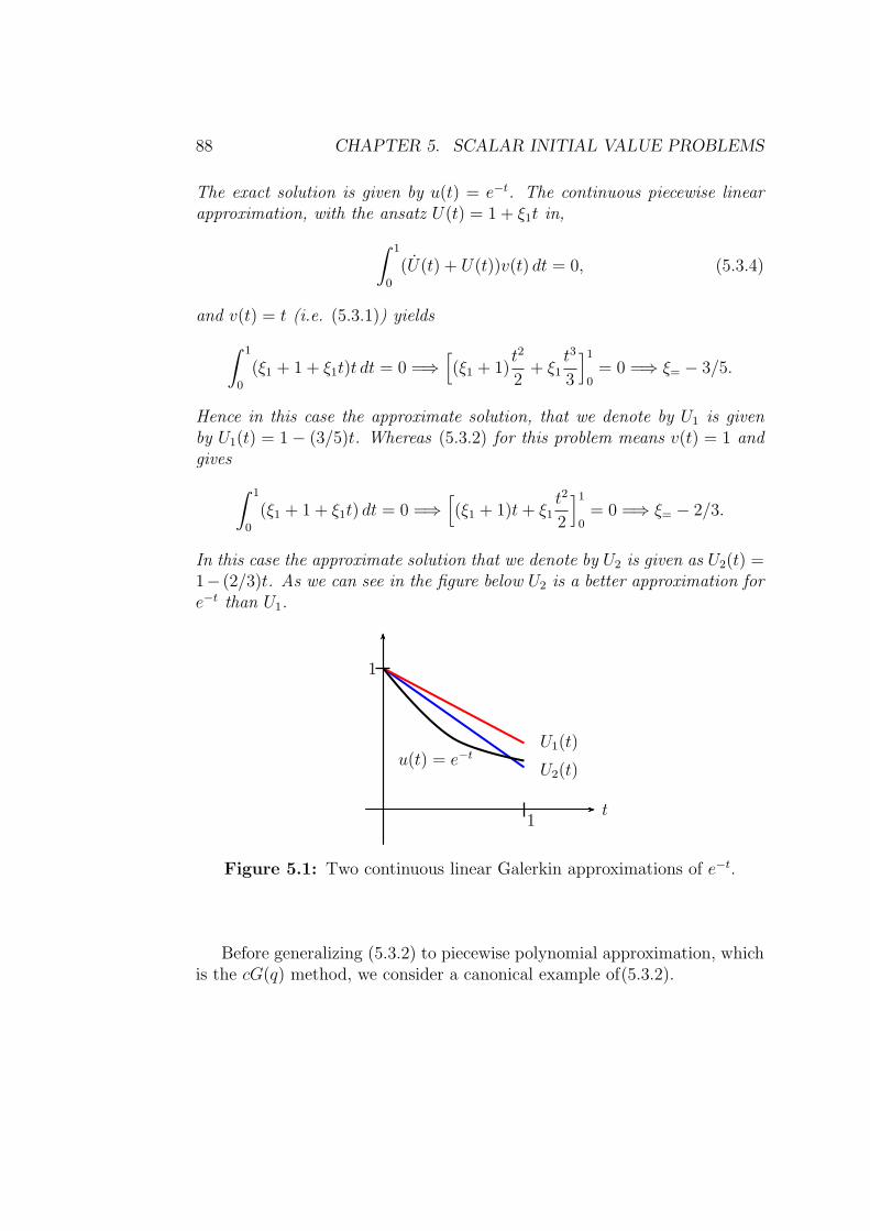
88 CHAPTER 5. SCALAR INITIAL VALUE PROBLEMS
The exact solution is given by u(t) = e−t. The continuous piecewise linearapproximation, with the ansatz U(t) = 1 + ξ1t in,
∫ 1
0
(U(t) + U(t))v(t) dt = 0, (5.3.4)
and v(t) = t (i.e. (5.3.1)) yields
∫ 1
0
(ξ1 + 1 + ξ1t)t dt = 0 =⇒[(ξ1 + 1)
t2
2+ ξ1
t3
3
]10= 0 =⇒ ξ= − 3/5.
Hence in this case the approximate solution, that we denote by U1 is givenby U1(t) = 1− (3/5)t. Whereas (5.3.2) for this problem means v(t) = 1 andgives
∫ 1
0
(ξ1 + 1 + ξ1t) dt = 0 =⇒[(ξ1 + 1)t+ ξ1
t2
2
]10= 0 =⇒ ξ= − 2/3.
In this case the approximate solution that we denote by U2 is given as U2(t) =1− (2/3)t. As we can see in the figure below U2 is a better approximation fore−t than U1.
1
1
U1(t)
U2(t)
t
u(t) = e−t
Figure 5.1: Two continuous linear Galerkin approximations of e−t.
Before generalizing (5.3.2) to piecewise polynomial approximation, whichis the cG(q) method, we consider a canonical example of(5.3.2).
5.3. GALERKIN FINITE ELEMENT METHODS FOR IVP 89
Example 5.5. Consider (5.3.2) with q = 1, then choosing v ≡ 1, yields
∫ T
0
(U + aU)vdt =
∫ T
0
(U + aU)dt = U(T )− U(0) +
∫ T
0
aU(t)dt (5.3.5)
Here U(t), as a linear function, is given by
U(t) = U(0)T − t
T+ U(T )
t
T. (5.3.6)
Inserting (5.3.6) into (5.3.5) we get
U(T )− U(0) +
∫ T
0
a(U(0)
T − t
T+ U(T )
t
T
)dt =
∫ T
0
f dt, (5.3.7)
which is an equation for the unknown quantity U(T ). Thus, using (5.3.6) witha given U(0), we get the linear approximation U(t) for all t ∈ [0, T ]. Belowwe generalize this example to piecewise linear approximation and demonstratethe iteration procedure for the cG(1) scheme.
The cG(1) AlgorithmFor a partition Tk of the interval [0, T ] into subintervals Ik = (tk−1, tk], weperform the following steps:
(1) Given U(0) = U0 = u0 and a source term f , apply (5.3.7) to the firstsubinterval (0, t1] and compute U(t1). Then, using (5.3.6) one getsU(t), ∀t ∈ [0, t1].
(2) Assume that we have computed Uk−1 := U(tk−1). Hence, Uk−1 andf are now considered as data. Now we consider the problem on thesubintervals Ik = (tk−1, tk], and compute the unknown Uk := U(tk)from the local version of (5.3.7),
Uk − Uk−1 +
∫ tk
tk−1
a( tk − t
tk − tk−1
Uk−1 +t− tk−1
tk − tk−1
Uk
)dt =
∫ tk
tk−1
fdt.
Having both Uk−1 and Uk, by linearity, we get U(t) for t ∈ Ik. To get thecontinuous piecewise linear approximation in the whole interval [0, tN ],step (2) is performed in successive subintervals Ik, k = 2, . . . , N .
90 CHAPTER 5. SCALAR INITIAL VALUE PROBLEMS
The cG(q) method
The Global continuous Galerkin method of degree q, formulated on a parti-tion Tk, 0 = t0 < t1 < . . . < tN = T of the interval (0, T ), is referred to as
the cG(q) method and reads as: find U(t) ∈ V(q)k , such that U(0) = u0, and
∫ tN
0
(U + aU)wdt =
∫ tN
0
fwdt, ∀w ∈ W(q−1)k , (5.3.8)
where
V(q)k = v : v continuous, piecewise polynomial of degree ≤ q on Tk,
W(q−1)k = w : w discontinuous, piecewise polynomial, deg w ≤ q − 1 on Tk.
So, the difference between the global continuous Galerkin method and cG(q)is that now we have piecewise polynomials on a partition of [0, T ] rather thanglobal polynomials in the whole interval [0, T ].
5.3.2 The discontinuous Galerkin method
We start presenting the global discontinuous Galerkin method of degree q:find U(t) ∈ Pq(0, T ) such that
∫ T
0
(U + aU)vdt+ (U(0)− u(0))v(0) =
∫ T
0
fvdt, ∀v ∈ Pq(0, T ). (5.3.9)
This approach gives up the requirement that U(t) satisfies the initial condi-tion. Instead, the initial condition is imposed in a variational sense by theterm (U(0) − u(0))v(0). As in the cG(q) case, to derive the discontinuousGalerkin method of degree q: dG(q) scheme, the above strategy can be for-mulated for the subintervals in a partition Tk. To this end, we recall thenotation for the right/left limits: v±n = lim
s→0+v(tn ± s) and the corresponding
jump term [vn] = v+n − v−n at time level t = tn. Then, the dG(q) method for(5.0.1) reads as follows: for n = 1, . . . , N ; find U(t) ∈ Pq(tn−1, tn) such that
∫ tn
tn−1
(U + aU)vdt+ U+n−1v
+n−1 =
∫ tn
tn−1
fvdt+ U−n−1v
+n−1, ∀v ∈ Pq(tn−1, tn).
(5.3.10)

5.3. GALERKIN FINITE ELEMENT METHODS FOR IVP 91
tn−1 tn tn+1t
kn
v−n
[vn]
v+n
•
•
Figure 5.2: The jump [vn] and the right and left limits v±n
Example 5.6 (dG(0)). Let q = 0, then v is constant generated by the singlebasis function: v ≡ 1. Further, we have U(t) = Un = U+
n−1 = U−n on
In = (tn−1, tn], and U ≡ 0. Thus, for q = 0 (5.3.10) yields the followingdG(0) formulation: for n = 1, . . . , N ; find piecewise constants Un such that
∫ tn
tn−1
aUndt+ Un =
∫ tn
tn−1
fdt+ Un−1. (5.3.11)
Summing over n in (5.3.10), we get the following general dG(q) formulation:
Find U(t) ∈ W(q)k , with U−
0 = u0 such that
N∑
n=1
∫ tn
tn−1
(U + aU)wdt+N∑
n=1
[Un−1]w+n−1 =
∫ tN
0
fwdt, ∀w ∈ W(q)k . (5.3.12)
Remark 5.3. One can show that cG(1) converges faster than dG(0), whereasdG(0) has better stability properties than cG(1): More specifically, in theparabolic case when a > 0 is constant and (f ≡ 0) we can easily verifythat (see Exercise 6.10 at the end of this chapter) the dG(0) solution Un
corresponds to the Backward Euler scheme
Un =( 1
1 + ak
)n
u0,
and the cG(1) solution Un is given by the Crank-Nicolson scheme:
Un =(1− 1
2ak
1 + 12ak
)n
u0,
where k is the constant time step.

92 CHAPTER 5. SCALAR INITIAL VALUE PROBLEMS
5.4 Exercises
Problem 5.1. (a) Derive the stiffness matrix and load vector in piecewisepolynomial (of degree q) approximation for the ODE of population dynamics:
u(t) = λu(t), for 0 < t ≤ 1, u(0) = u0.
(b) Let λ = 1 and u0 = 1 and determine the approximate solution U(t), forq = 1 and q = 2.
Problem 5.2. Consider the initial value problem
u(t) + a(t)u(t) = f(t), 0 < t ≤ T, u(0) = u0.
Show that if a(t) = 1, f(t) = 2 sin(t), then we haveu(t) = sin(t)− cos(t) =
√2 sin(t− π/2).
Problem 5.3. Compute the solution for
u(t) + a(t)u(t) = t2, 0 < t ≤ T, u(0) = 1,
corresponding to(a) a(t) = 4, (b) a(t) = −t.
Problem 5.4. Compute the cG(1) approximation for the differential equa-tions in the above problem. In each case, determine the condition on the stepsize that guarantees that U exists.
Problem 5.5. Without using the solution Theorem 5.1, prove that if a(t) ≥ 0then, a continuously differentiable solution of (5.0.1) is unique.
Problem 5.6. Consider the initial value problem
u(t) + a(t)u(t) = f(t), 0 < t ≤ T, u(0) = u0.
Show that for a(t) > 0, and for N = 1, 2, . . . , the piecewise linear approxi-mate solution U for this problem satisfies the error estimate
|u(tN)− UN | ≤ max[0,tN ]
|k(U + aU − f)|, k = kn, for tn−1 < t ≤ tn.

5.4. EXERCISES 93
Problem 5.7. Consider the initial value problem
u(t) + au(t) = 0, t > 0, u(0) = u0, (a = constant).
Assume a constant time step k and verify the iterative formulas for dG(0)and cG(1) approximations U and U , respectively: i.e.
Un =( 1
1 + ak
)n
u0, Un =(1− ak/2
1 + ak/2
)n
u0.
Problem 5.8. Assume that∫
Ij
f(s) ds = 0, for j = 1, 2, . . . ,
where Ij = (tj−1, tj), tj = jk with k being a positive constant. Prove that ifa(t) ≥ 0, then the solution for (5.0.1) satisfies
|u(t)| ≤ e−A(t)|u0|+ max0≤s≤t
|kf(s)|.
Problem 5.9. Formulate a continuous Galerkin method using piecewise poly-nomials based on the original global Galerkin method.
Problem 5.10. Formulate the dG(1) method for the differential equationsspecified in Problem 5.3.
Problem 5.11. Write out the a priori error estimates for the equationsspecified in Problem 5.3.
Problem 5.12. Use the a priori error bound to show that the residual of thedG(0) approximation satisfies R(U) = O(1).
Problem 5.13. Prove the following stability estimate for the dG(0) methoddescribed by (5.3.12),
|UN |2 +N−1∑
n=0
|[Un]|2 ≤ |u0|2.

94 CHAPTER 5. SCALAR INITIAL VALUE PROBLEMS

Chapter 6
Initial Boundary ValueProblems in 1d
A large class of phenomena in nature, science and technology, such as seasonalperiods, heat distribution, wave propagation, etc, are varying both in space andtime. To describe these phenomena in a physical domain requires the knowledgeof their initial status, as well as information on the boundary of the domain, orasymptotic behavior in the case of unbounded domains. Problems that modelsuch properties are called initial boundary value problems. In this chapter we shallstudy the two most important equations of this type: namely, the heat equationand the wave equation in one space dimension. We also address (briefly) theone-space dimensional time-dependent convection-diffusion problem.
6.1 Heat equation in 1d
In this section we focus on some basic L2-stability and finite element error es-timates for the, time-dependent, one-space dimensional heat equation. Here,to illustrate, we consider an example of an initial boundary value problem(IBVP) for the one-dimensional heat flux, viz
u− u′′ = f(x, t), 0 < x < 1, t > 0,
u(x, 0) = u0(x), 0 < x < 1,
u(0, t) = ux(1, t) = 0, t > 0.
(6.1.1)
95

96 CHAPTER 6. INITIAL BOUNDARY VALUE PROBLEMS IN 1Du(x, t)
x
t
u0(x)
tn−1
tn
Figure 6.1: A decreasing temperature profile with data u(0, t) = u(1, t) = 0.
Example 6.1. Describe the physical meaning of the functions and parame-ters in the problem (6.1.1), when f = 20− u.
Answer: The problem is an example of heat conduction where
u(x, t), means the temperature at the point x and time t.
u(x, 0) = u0(x), is the initial temperature at time t = 0.
u(0, t) = 0, means fixed temperature at the boundary point x = 0.
u′(1, t) = 0, means isolated boundary at the boundary point x = 1
(where no heat flux occurs).
f = 20− u, is the heat source, in this case a control system to force
u→ 20.
Remark 6.1. Observe that it is possible to generalize (6.1.1) to a u dependentsource term f , e.g. as in the above example where f = 20− u.
6.1.1 Stability estimates
We shall derive a general stability estimate for the mixed (Dirichlet at oneend point and Neumann in the other) initial boundary value problem above,

6.1. HEAT EQUATION IN 1D 97
prove a one-dimensional version of the Poincare inequality and finally derivesome stability estimates in the homogeneous (f ≡ 0) case.
Theorem 6.1. The IBVP (6.1.1) satisfies the stability estimates
||u(·, t)|| ≤ ||u0||+∫ t
0
||f(·, s)|| ds, (6.1.2)
||u′(·, t)||2 ≤ ||u′0||2 +∫ t
0
||f(·, s)||2 ds, (6.1.3)
where u0 and u′0 are assumed to be L2(I) functions with I = (0, 1). Notefurther that, here || • (·, t)|| is the time dependent L2 norm:
||w(·, s)|| := ||w(·, s)||L2(0,1) =(∫ 1
0
||w(x, s)||2 dx)1/2
.
Proof. Multiply the equation in (6.1.1) by u and integrate over (0, 1) to get
∫ 1
0
uu dx−∫ 1
0
u′′u dx =
∫ 1
0
fu dx. (6.1.4)
Note that uu = 12
ddtu2. Hence, integration by parts in the second integral
yields
1
2
d
dt
∫ 1
0
u2 dx+
∫ 1
0
(u′)2 dx− u′(1, t)u(1, t) + u′(0, t)u(0, t) =
∫ 1
0
fu dx.
Then, using boundary conditions and Cauchy-Schwarz’ inequality yields
||u|| ddt||u||+ ||u′||2 =
∫ 1
0
fu dx ≤ ||f || ||u||. (6.1.5)
Now since ||u′||2 ≥ 0, consequently ||u|| ddt||u|| ≤ ||f || ||u||, and thus
d
dt||u|| ≤ ||f ||. (6.1.6)
Relabeling the variable from t to s, and integrating over time we end up with
||u(·, t)|| − ||u(·, 0)|| ≤∫ t
0
||f(·, s)|| ds, (6.1.7)

98 CHAPTER 6. INITIAL BOUNDARY VALUE PROBLEMS IN 1D
which yields the first assertion (6.1.2) of the theorem. To prove (6.1.3) wemultiply the differential equation by u, integrate over (0, 1), and use integra-tion by parts so that we have on the left hand side∫ 1
0
(u)2 dx−∫ 1
0
u′′u dx = ||u||2 +∫ 1
0
u′u′ dx− u′(1, t)u(1, t) + u′(0, t)u(0, t).
Then, since u(0, t) = 0 =⇒ u(0, t) = 0, we have
||u||2 + 1
2
d
dt||u′||2 =
∫ 1
0
fu dx ≤ ||f || ||u|| ≤ 1
2
(||f ||2 + ||u||2
), (6.1.8)
where in the last step we used Cauchy-Schwarz’ inequality. Hence,
1
2||u||2 + 1
2
d
dt||u′||2 ≤ 1
2||f ||2, (6.1.9)
and therefore, evidently,d
dt||u′||2 ≤ ||f ||2. (6.1.10)
Finally, integrating over (0, t) we get the second assertion of the theorem:
||u′(·, t)||2 − ||u′(·, 0)||2 ≤∫ t
0
||f(·, s)||2 ds, (6.1.11)
and the proof is complete.
To proceed we give a proof of the Poincare inequality (in 1d) which is oneof the most useful inequalities in PDE and analysis.
Theorem 6.2 (The Poincare inequality in 1 − d). Assume that u and u′
are square integrable functions on an interval [0, L]. Then, there exists aconstant CL, independent of u, but dependent on L, such that if u(0) = 0,
∫ L
0
u(x)2 dx ≤ CL
∫ L
0
u′(x)2 dx, i.e. ||u|| ≤√CL||u′||. (6.1.12)
Proof. For x ∈ [0, L] we may write
u(x) =
∫ x
0
u′(y) dy ≤∫ x
0
|u′(y)| dy =
∫ x
0
|u′(y)| · 1 dy
≤(∫ x
0
|u′(y)|2 dy)1/2
·(∫ x
0
12dy)1/2
≤(∫ L
0
|u′(y)|2 dy)1/2
·(∫ L
0
12dy)1/2
=√L(∫ L
0
|u′(y)|2 dy)1/2
,
6.1. HEAT EQUATION IN 1D 99
where in the last step we used the Cauchy-Schwarz inequality. Thus, squaringboth sides and integrating, we get
∫ L
0
u(x)2 dx ≤∫ L
0
L(∫ L
0
|u′(y)|2 dy)dx = L2
∫ L
0
|u′(y)|2 dy, (6.1.13)
and hence
||u|| ≤ L||u′||. (6.1.14)
Remark 6.2. The constant CL = L2 indicates that the Poincare inequalityis valid for arbitrary bounded intervals, but not for unbounded intervals. Ifu(0) 6= 0 and, for simplicity L = 1, then by a similar argument as above weget the following version of the one-dimensional Poincare inequality:
||u||2L2(0,1)≤ 2
(u(0)2 + ||u′||2L2(0,1)
). (6.1.15)
Theorem 6.3 (Stability of the homogeneous heat equation). The initialboundary value problem for the heat equation
u− u′′ = 0, 0 < x < 1, t > 0
u(0, t) = ux(1, t) = 0, t > 0
u(x, 0) = u0(x), 0 < x < 1,
(6.1.16)
satisfies the following stability estimates
a)d
dt||u||2 + 2||u′||2 = 0, b) ||u(·, t)|| ≤ e−t||u0||.
Proof. a) Multiply the equation by u and integrate over x ∈ (0, 1), to get
0 =
∫ 1
0
(u−u′′)u dx =
∫ 1
0
uu dx+
∫ 1
0
(u′)2 dx−u′(1, t)u(1, t)+u′(0, t)u(0, t),
where we used integration by parts. Using the boundary data we then have
1
2
d
dt
∫ 1
0
u2 dx+
∫ 1
0
(u′)2 dx =1
2
d
dt||u||2 + ||u′||2 = 0.

100 CHAPTER 6. INITIAL BOUNDARY VALUE PROBLEMS IN 1D
This gives the proof of a). As for the proof of b), using a) and the Poincareinequality, with L = 1, i.e., ||u|| ≤ ||u′|| we get
d
dt||u||2 + 2||u||2 ≤ 0. (6.1.17)
Multiplying both sides of (6.1.17) by the integrating factor e2t yields
d
dt
(||u||2e2t
)=
( ddt||u||2 + 2||u||2
)e2t ≤ 0. (6.1.18)
We replace t by s and integrate with respect to s, over (0, t), to obtain
∫ t
0
d
ds
(||u||2e2s
)ds = ||u(·, t)||2e2t − ||u(·, 0)||2 ≤ 0. (6.1.19)
This yields
||u(·, t)||2 ≤ e−2t||u0||2 =⇒ ||u(·, t)|| ≤ e−t||u0||, (6.1.20)
and completes the proof.
6.1.2 FEM for the heat equation
We consider the one-dimensional heat equation with Dirichlet boundary data:
u− u′′ = f, 0 < x < 1, t > 0,
u(0, t) = u(1, t) = 0, t > 0,
u(x, 0) = u0(x), 0 < x < 1.
(6.1.21)
The Variational formulation for this problem reads as follows: For every timeinterval In = (tn−1, tn], find u(x, t), x ∈ (0, 1), t ∈ In, such that
∫
In
∫ 1
0
(uv + u′v′)dxdt =
∫
In
∫ 1
0
fvdxdt, ∀v : v(0, t) = v(1, t) = 0. (VF)
A piecewise linear Galerkin finite element method: cG(1) − cG(1) is thenformulated as: for each time interval In := (tn−1, tn], with tn − tn−1 = kn, let
U(x, t) = Un−1(x)Ψn−1(t) + Un(x)Ψn(t), (6.1.22)

6.1. HEAT EQUATION IN 1D 101
where
Ψn(t) =t− tn−1
kn, Ψn−1(t) =
tn − t
kn, (6.1.23)
and
Un(x) = Un,1ϕ1(x) + Un,2ϕ2(x) + . . .+ Un,mϕm(x), n = n− 1, n (6.1.24)
with ϕj being the usual continuous, piecewise linear finite element basisfunctions (hat-functions) corresponding to a partition of Ω = (0, 1), with0 = x0 < · · · < xℓ < xℓ+1 < · · · < xm+1 = 1, and ϕj(xi) := δij. Now theGalerkin method (FEM) is to determine the unknown coefficients Un,ℓ in theabove representation for U (U is a continuous, piecewise linear function bothin space and time variables) that satisfies the following discrete variationalformulation: Find U(x, t) given by (6.1.22) such that
∫
In
∫ 1
0
(Uϕi + U ′ϕ′i) dxdt =
∫
In
∫ 1
0
fϕi dxdt, i = 1, 2, . . . ,m. (6.1.25)
Note that, on In = (tn−1, tn] and with Un(x) := U(x, tn) and Un−1(x) :=U(x, tn−1),
U(x, t) = Un−1(x)Ψn−1(t) + Un(x)Ψn(t) =Un − Un−1
kn. (6.1.26)
Further differentiating (6.1.22) with respect to x we have
U ′(x, t) = U ′n−1(x)Ψn−1(t) + U ′
n(x)Ψn(t). (6.1.27)
Inserting (6.1.26) and (6.1.27) into (6.1.25) we get using the identities,∫Indt =
kn and∫InΨndt =
∫InΨn−1dt = kn/2 that,
∫ 1
0
Unϕidx
︸ ︷︷ ︸M ·Un
−∫ 1
0
Un−1ϕi dx
︸ ︷︷ ︸M ·Un−1
+
∫
In
Ψn−1 dt
︸ ︷︷ ︸kn/2
∫ 1
0
U ′n−1ϕ
′i dx
︸ ︷︷ ︸S·Un−1
+
∫
In
Ψn dt
︸ ︷︷ ︸kn/2
∫ 1
0
U ′nϕ
′i dx
︸ ︷︷ ︸S·Un
=
∫
In
∫ 1
0
fϕi dxdt
︸ ︷︷ ︸Fn
.
(6.1.28)
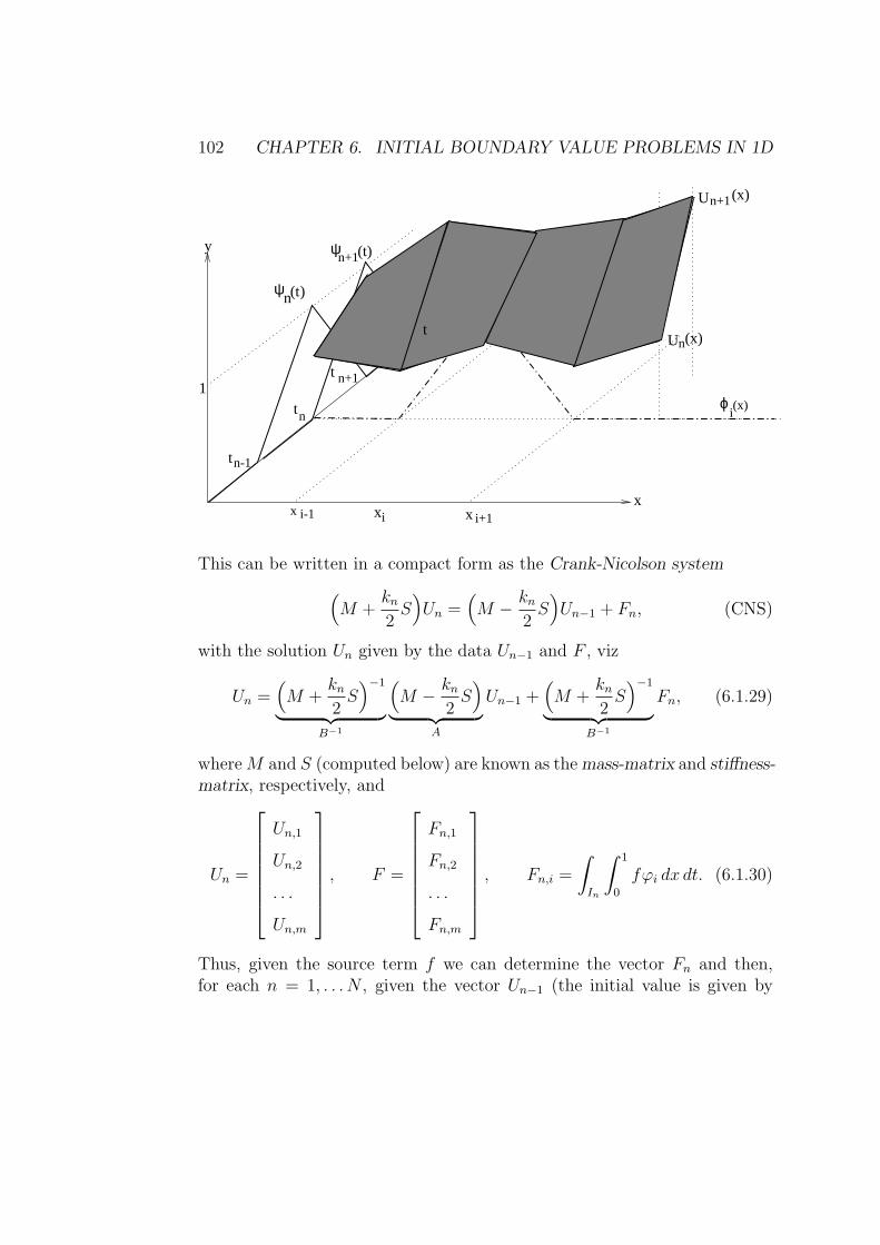
102 CHAPTER 6. INITIAL BOUNDARY VALUE PROBLEMS IN 1D
x
y
t
x
t
t
n-1
nt
n+1
i
)ψ (tn
1
U
Un(x)
n+1(x)
ψn+1(t)
ϕi(x)
x xi-1 i+1
This can be written in a compact form as the Crank-Nicolson system
(M +
kn2S)Un =
(M − kn
2S)Un−1 + Fn, (CNS)
with the solution Un given by the data Un−1 and F , viz
Un =(M +
kn2S)−1
︸ ︷︷ ︸B−1
(M − kn
2S)
︸ ︷︷ ︸A
Un−1 +(M +
kn2S)−1
︸ ︷︷ ︸B−1
Fn, (6.1.29)
whereM and S (computed below) are known as themass-matrix and stiffness-matrix, respectively, and
Un =
Un,1
Un,2
. . .
Un,m
, F =
Fn,1
Fn,2
. . .
Fn,m
, Fn,i =
∫
In
∫ 1
0
fϕi dx dt. (6.1.30)
Thus, given the source term f we can determine the vector Fn and then,for each n = 1, . . . N , given the vector Un−1 (the initial value is given by

6.1. HEAT EQUATION IN 1D 103
U0,j := u0(xj)) we may use the CNS to compute Un,ℓ, ℓ = 1, 2, . . . m (mnodal values of U at the xj : s, and at the time level tn).
We now return to the computation of the matrix entries for M and S, fora uniform partition (all subintervals are of the same length) of the intervalI = (0, 1). Note that differentiating (6.1.24) with respect to x, yields
U ′n(x) = Un,1ϕ
′1(x) + Un,2ϕ
′2(x) + . . .+ Un,mϕ
′m(x). (6.1.31)
Hence, for i = 1, . . . ,m, the rows in the system of equations are given by
∫ 1
0
U ′nϕ
′i =
(∫ 1
0
ϕ′iϕ
′1
)Un,1 +
(∫ 1
0
ϕ′iϕ
′2
)Un,2 + . . .+
(∫ 1
0
ϕ′iϕ
′m
)Un,m,
which can be written in matrix form as
SUn =
∫ 1
0ϕ′1ϕ
′1
∫ 1
0ϕ′1ϕ
′2 . . .
∫ 1
0ϕ′1ϕ
′m
∫ 1
0ϕ′2ϕ
′1
∫ 1
0ϕ′2ϕ
′2 . . .
∫ 1
0ϕ′2ϕ
′m
. . . . . . . . . . . .∫ 1
0ϕ′mϕ
′1
∫ 1
0ϕ′mϕ
′2 . . .
∫ 1
0ϕ′mϕ
′m
Un,1
Un,2
. . .
Un,m
. (6.1.32)
Thus, S is just the stiffness matrix Aunif computed in Chapter 2:
S =1
h
2 −1 0 0 . . . 0
−1 2 −1 0 . . . 0
. . . . . . . . . . . . . . . . . .
0 . . . . . . −1 2 −1
0 . . . . . . . . . −1 2
. (6.1.33)
A non-uniform partition yields a matrix of the form A in Chapter 2.Similarly, recalling the notation for the mass matrix M i in (6.1.28), we have
[MUn]i =
∫ 1
0
Unϕi, i = 1, . . . ,m. (6.1.34)
Hence, to compute the mass matrix M one should drop all derivatives fromthe general form of the matrix for S given by (6.1.32). In other words unlike

104 CHAPTER 6. INITIAL BOUNDARY VALUE PROBLEMS IN 1D
the form [SUn]i =∫ 1
0U ′nϕ
′i, MUn does not involve any derivatives, neither in
Un nor in ϕi. Consequently
M =
∫ 1
0ϕ1ϕ1
∫ 1
0ϕ1ϕ2 . . .
∫ 1
0ϕ1ϕm
∫ 1
0ϕ2ϕ1
∫ 1
0ϕ2ϕ2 . . .
∫ 1
0ϕ2ϕm
. . . . . . . . . . . .∫ 1
0ϕmϕ1
∫ 1
0ϕmϕ2 . . .
∫ 1
0ϕmϕm
. (6.1.35)
For a uniform partition, we have computed this mass matrix in Chapter 4:
M = h
23
16
0 0 . . . 0
16
23
16
0 . . . 0
. . . . . . . . . . . . . . . . . .
0 . . . . . . 16
23
16
0 . . . . . . . . . 16
23
=h
6
4 1 0 0 . . . 0
1 4 1 0 . . . 0
. . . . . . . . . . . . . . . . . .
0 . . . . . . 1 4 1
0 . . . . . . . . . 1 4
.
6.1.3 Exercises
Problem 6.1. Derive a system of equations, as (6.1.29), for cG(1)−dG(0):with the discontinuous Galerkin approximation dG(0) in time with piecewiseconstants.
Problem 6.2. Let ‖ · ‖ denote the L2(0, 1)-norm. Consider the problem
−u′′ = f, 0 < x < 1,
u′(0) = v0, u(1) = 0.
a) Show that |u(0)| ≤ ‖u′‖ and ‖u‖ ≤ ‖u′‖.b) Use a) to show that ‖u′‖ ≤ ‖f‖+ |v0|.Problem 6.3. Assume that u = u(x) satisfies
∫ 1
0
u′v′dx =
∫ 1
0
fv dx, for all v(x) such that v(0) = 0. (6.1.36)
Show that −u′′ = f for 0 < x < 1 and u′(1) = 0.Hint: See previous chapters.

6.1. HEAT EQUATION IN 1D 105
Problem 6.4 (Generalized Poincare). Show that for a continuously differ-entiable function v defined on (0, 1) we have that
||v||2 ≤ v(0)2 + v(1)2 + ||v′||2.Hint: Use partial integration for
∫ 1/2
0v(x)2 dx and
∫ 1
1/2v(x)2 dx and note that
(x− 1/2) has the derivative 1.
Problem 6.5. Let ‖ · ‖ denote the L2(0, 1)-norm. Consider the followingheat equation
u− u′′ = 0, 0 < x < 1, t > 0,
u(0, t) = ux(1, t) = 0, t > 0,
u(x, 0) = u0(x), 0 < x < 1.
a) Show that the norms: ||u(·, t)|| and ||u′(·, t)|| are non-increasing in time.
||u|| =( ∫ 1
0u(x)2 dx
)1/2
.
b) Show that ||u′(·, t)|| → 0, as t→ ∞.
c) Give a physical interpretation for a) and b).
Problem 6.6. Consider the inhomogeneous problem:
u− εu′′ = f, 0 < x < 1, t > 0,
u(0, t) = ux(1, t) = 0, t > 0,
u(x, 0) = u0(x), 0 < x < 1.
where f = f(x, t).a) Show the stability estimate
||u(·, t)|| ≤∫ t
0
||f(·, s)|| ds.
b) Show that for the corresponding stationary (u ≡ 0) problem we have
||u′|| ≤ 1
ε||f ||.
Problem 6.7. Give an a priori error estimate for the following problem:
(au′′)′′ = f, 0 < x < 1, u(0) = u′(0) = u(1) = u′(1) = 0,
where a(x) > 0 on the interval I = (0, 1).

106 CHAPTER 6. INITIAL BOUNDARY VALUE PROBLEMS IN 1D
6.2 The wave equation in 1d
The theoretical study of the wave equation has some basic differences com-pared to that of the heat equation. Some important aspects in this regardare given in extended version of these notes. In our study here, the finiteelement procedure for the wave equation is, mainly, the same as for that ofthe heat equation outlined in the previous section. We start with an exampleof the homogeneous wave equation, as an initial-boundary value problem:
u− u′′ = 0, 0 < x < 1 t > 0 (DE)
u(0, t) = 0, u(1, t) = 0 t > 0 (BC)
u(x, 0) = u0(x), u(x, 0) = v0(x), 0 < x < 1. (IC)
(6.2.1)
Theorem 6.4 (conservation of energy). For the equation (6.2.1) we have
1
2||u||2 + 1
2||u′||2 = 1
2||v0||2 +
1
2||u′0||2 = Constant, (6.2.2)
where
||w||2 = ||w(·, t)||2 =∫ 1
0
|w(x, t)|2 dx. (6.2.3)
Proof. We multiply the equation by u and integrate over I = (0, 1) to get
∫ 1
0
u udx−∫ 1
0
u′′ u dx = 0. (6.2.4)
Using integration by parts and the boundary data we obtain
∫ 1
0
1
2
∂
∂t
(u)2
dx+
∫ 1
0
u′ (u)′ dx−[u′(x, t)u(x, t)
]10
=
∫ 1
0
1
2
∂
∂t
(u)2
dx+
∫ 1
0
1
2
∂
∂t
(u′)2
dx
=1
2
d
dt
(||u||2 + ||u′||2
)= 0.
(6.2.5)
Thus, we have that the quantity
1
2||u||2 + 1
2||u′||2 = Constant, independent of t. (6.2.6)

6.2. THE WAVE EQUATION IN 1D 107
Therefore the total energy is conserved. We recall that 12||u||2 is the kinetic
energy, and 12||u′||2 is the potential (elastic) energy.
Problem 6.8. Show that ‖(u)′‖2 + ‖u′′‖2 = constant, independent of t.Hint: Differentiate the equation with respect to x and multiply by u, . . . .Alternatively: Multiply (DE): u− u′′ = 0, by −(u)′′ and integrate over I.
Problem 6.9. Derive a total conservation of energy relation using the Robintype boundary condition: u′ + u = 0.
6.2.1 Wave equation as a system of PDEs
We rewrite the wave equation as a system of differential equations. To thisapproach, we consider solving
u− u′′ = 0, 0 < x < 1, t > 0,
u(0, t) = 0, u′(1, t) = g(t), t > 0,
u(x, 0) = u0(x), u(x, 0) = v0(x), 0 < x < 1,
(6.2.7)
where we let u = v, and reformulate the problem as:
u− v = 0, (Convection)
v − u′′ = 0, (Diffusion).(6.2.8)
We may now set w = (u, v)t and rewrite the system (6.2.8) as w + Aw = 0:
w + Aw =
u
v
+
0 −1
− ∂2
∂x2 0
u
v
=
0
0
. (6.2.9)
In other words, the matrix differential operator is given by
A =
0 −1
− ∂2
∂x2 0
.
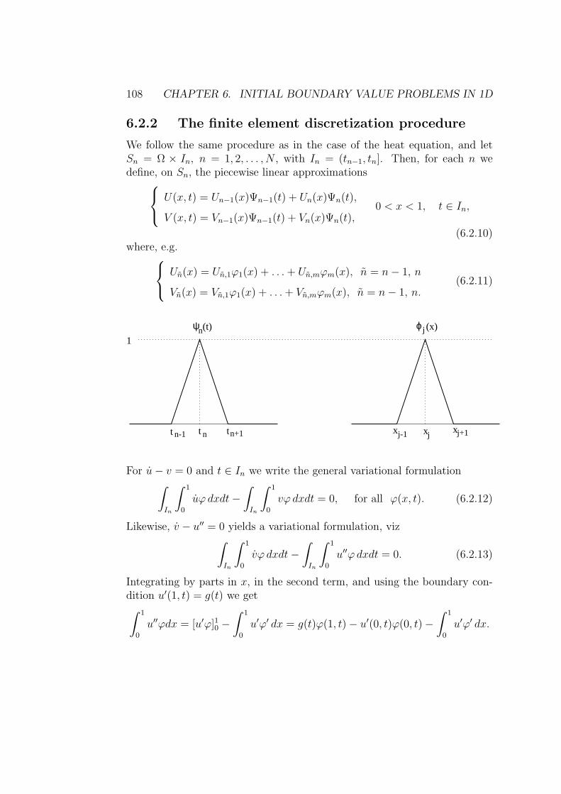
108 CHAPTER 6. INITIAL BOUNDARY VALUE PROBLEMS IN 1D
6.2.2 The finite element discretization procedure
We follow the same procedure as in the case of the heat equation, and letSn = Ω × In, n = 1, 2, . . . , N , with In = (tn−1, tn]. Then, for each n wedefine, on Sn, the piecewise linear approximations
U(x, t) = Un−1(x)Ψn−1(t) + Un(x)Ψn(t),
V (x, t) = Vn−1(x)Ψn−1(t) + Vn(x)Ψn(t),0 < x < 1, t ∈ In,
(6.2.10)where, e.g.
Un(x) = Un,1ϕ1(x) + . . .+ Un,mϕm(x), n = n− 1, n
Vn(x) = Vn,1ϕ1(x) + . . .+ Vn,mϕm(x), n = n− 1, n.(6.2.11)
1
ψn(t) ϕ j (x)
t n-1 t n tn+1 x x xj-1 j+1j
For u− v = 0 and t ∈ In we write the general variational formulation∫
In
∫ 1
0
uϕ dxdt−∫
In
∫ 1
0
vϕ dxdt = 0, for all ϕ(x, t). (6.2.12)
Likewise, v − u′′ = 0 yields a variational formulation, viz∫
In
∫ 1
0
vϕ dxdt−∫
In
∫ 1
0
u′′ϕdxdt = 0. (6.2.13)
Integrating by parts in x, in the second term, and using the boundary con-dition u′(1, t) = g(t) we get∫ 1
0
u′′ϕdx = [u′ϕ]10 −∫ 1
0
u′ϕ′ dx = g(t)ϕ(1, t)− u′(0, t)ϕ(0, t)−∫ 1
0
u′ϕ′ dx.

6.2. THE WAVE EQUATION IN 1D 109
Inserting the right hand side in (6.2.13) we get for all ϕ with ϕ(0, t) = 0:
∫
In
∫ 1
0
vϕ dxdt+
∫
In
∫ 1
0
u′ϕ′ dxdt =
∫
In
g(t)ϕ(1, t) dt. (6.2.14)
The corresponding cG(1)cG(1) finite element method reads as follows: Foreach n, n = 1, 2, . . . , N , find continuous piecewise linear functions U(x, t)and V (x, t), in a partition, 0 = x0 < x1 < · · · < xm = 1 of Ω = (0, 1), suchthat
∫
In
∫ 1
0
Un(x)− Un−1(x)
knϕj(x) dxdt
−∫
In
∫ 1
0
(Vn−1(x)Ψn−1(t) + Vn(x)Ψn(t)
)ϕj(x) dxdt = 0,
for j = 1, 2, . . . ,m,
(6.2.15)
and
∫
In
∫ 1
0
Vn(x)− Vn−1(x)
knϕj(x) dxdt
+
∫
In
∫ 1
0
(U ′n−1(x)Ψn−1(t) + U ′
n(x)Ψn(t))ϕ′j(x) dxdt
=
∫
In
g(t)ϕj(1) dt, for j = 1, 2, . . . ,m,
(6.2.16)
where U , U ′, V , and V ′ are computed using (6.2.10) with
ψn−1(t) =tn − t
kn, ψn(t) =
t− tn−1
kn, kn = tn − tn−1.
Thus, the equations (6.2.15) and (6.2.16) are reduced to the iterative forms:
∫ 1
0
Un(x)ϕj(x)dx
︸ ︷︷ ︸MUn
−kn2
∫ 1
0
Vn(x)ϕj(x)dx
︸ ︷︷ ︸MVn
=
∫ 1
0
Un−1(x)ϕj(x)dx
︸ ︷︷ ︸MUn−1
+kn2
∫ 1
0
Vn−1(x)ϕj(x) dx
︸ ︷︷ ︸MVn−1
, j = 1, 2, . . . ,m,

110 CHAPTER 6. INITIAL BOUNDARY VALUE PROBLEMS IN 1D
and
∫ 1
0
Vn(x)ϕj(x)dx
︸ ︷︷ ︸MVn
+kn2
∫ 1
0
U ′n(x)ϕ
′j(x) dx
︸ ︷︷ ︸SUn
=
∫ 1
0
Vn−1(x)ϕj(x) dx
︸ ︷︷ ︸MVn−1
−kn2
∫ 1
0
U ′n−1(x)ϕ
′j(x) dx
︸ ︷︷ ︸SUn−1
+gn, j = 1, 2, . . . ,m,
respectively, where we used (6.2.11) and as we computed earlier
S =1
h
2 −1 . . . 0
−1 2 −1 . . .
. . . . . . . . . . . .
0 −1 2 −1
0 0 −1 1
, M =h
6
4 1 . . . 0
1 4 1 . . .
. . . . . . . . . . . .
. . . 1 4 1
0 . . . 1 2
,
where
gn = (0, . . . , 0, gn,m)T , where gn,m =
∫
In
g(t) dt.
In compact form the vectors Un and Vn are determined by solving the linearsystem of equations:
MUn − kn2MVn =MUn−1 +
kn2MVn−1
kn2SUn +MVn = −kn
2SUn−1 +MVn−1 + gn,
(6.2.17)
which is a system of 2m equations with 2m unknowns:
M −kn
2M
kn2S M
︸ ︷︷ ︸A
Un
Vn
︸ ︷︷ ︸W
=
M kn
2M
−kn2S M
Un−1
Vn−1
+
0
gn
︸ ︷︷ ︸b
,
with W = A−1b, Un = W (1 : m) and Vn = W (m+ 1 : 2m).
6.2. THE WAVE EQUATION IN 1D 111
6.2.3 Exercises
Problem 6.10. Derive the corresponding linear system of equations in thecase of time discretization with dG(0).
Problem 6.11 (discrete conservation of energy). Show that cG(1)-cG(1) forthe wave equation in system form with g(t) = 0, conserves energy: i.e.
‖U ′n‖2 + ‖Vn‖2 = ‖U ′
n−1‖2 + ‖Vn−1‖2. (6.2.18)
Hint: Multiply the first equation by (Un−1 + Un)tSM−1 and the second equa-
tion by (Vn−1+Vn)t and add up. Use then, e.g., the fact that U t
nSUn = ‖U ′n‖2,
where
Un =
Un,1
Un,2
. . .
Un,m
, and Un = Un(x) = Un,1(x)ϕ1(x) + . . .+ Un,m(x)ϕm(x).
Problem 6.12. Consider the wave equation
u− u′′ = 0, x ∈ R, t > 0,
u(x, 0) = u0(x), x ∈ R,
u(x, 0) = v0(x), x ∈ R.
(6.2.19)
Plot the graph of u(x, 2) in the following cases.a) v0 = 0 and
u0(x) =
1, x < 0,
0, x > 0.
b) u0 = 0, and
v0(x) =
−1, −1 < x < 0,
1, 0 < x < 1,
0, |x| > 0.

112 CHAPTER 6. INITIAL BOUNDARY VALUE PROBLEMS IN 1D
Problem 6.13. Compute the solution for the wave equation
u− 4u′′ = 0, x > 0, t > 0,
u(0, t) = 0, t > 0,
u(x, 0) = u0(x), u(x, 0) = 0, x > 0.
(6.2.20)
Plot the solutions for the three cases t = 0.5, t = 1, t = 2, and with
u0(x) =
1, x ∈ [2, 3]
0, else(6.2.21)
Problem 6.14. Apply cG(1) time discretization directly to the wave equationby letting
U(x, t) = Un−1Ψn−1(t) + Un(x)Ψn(t), t ∈ In. (6.2.22)
Note that U is piecewise constant in time and comment on:∫
In
∫ 1
0
Uϕj dxdt
︸ ︷︷ ︸?
+
∫
In
∫ 1
0
u′ϕ′j dxdt
︸ ︷︷ ︸k2S(Un−1+Un)
=
∫
In
g(t)ϕj(1)dt
︸ ︷︷ ︸gn
, j = 1, 2, . . . ,m.
Problem 6.15. Construct a FEM for the problem
u+ u− u′′ = f, 0 < x < 1, t > 0,
u(0, t) = 0, u′(1, t) = 0, t > 0,
u(x, 0) = 0, u(x, 0) = 0, 0 < x < 1.
(6.2.23)
Problem 6.16. Determine the solution for the wave equation
u− c2u′′ = f, x > 0, t > 0,
u(x, 0) = u0(x), ut(x, 0) = v0(x), x > 0,
ux(1, t) = 0, u(0, t) = 0 t > 0,
in the following cases:
a) f = 0.
b) f = 1, u0 = 0, v0 = 0.

6.2. THE WAVE EQUATION IN 1D 113
Problem 6.17. Prove that the solution u of the convection-diffusion problem
−uxx + ux + u = f, in I = (0, 1), u(0) = u(1) = 0,
satisfies the following estimate(∫
I
u2φ dx)1/2
≤(∫
I
f 2φ dx)1/2
.
where φ(x) is a positive weight function defined on (0, 1) satisfying φ′(x) ≤ 0and −φ′(x) ≤ φ(x) for 0 ≤ x ≤ 1.
Problem 6.18. Let φ be a solution of the problem
−εφ′′ − 3φ′ + 2φ = e, φ′(0) = φ(1) = 0.
Let ‖ · ‖ denote the L2-norm on I. Show that there is a constant C such that
|φ(0)| ≤ C‖e‖, ‖εφ′′‖ ≤ C‖e‖.Problem 6.19. Use relevant interpolation theory estimates and prove an apriori error estimate for the cG(1) finite element method for the problem
−u′′ + u′ = f, in I = (0, 1), u(0) = u(1) = 0.
Problem 6.20. Prove an a priori error estimate for the cG(1) finite elementmethod for the problem
−u′′ + u′ + u = f, in I = (0, 1), u(0) = u(1) = 0.
Problem 6.21. Consider the problem
−εu′′ + xu′ + u = f, in I = (0, 1), u(0) = u′(1) = 0,
where ε is a positive constant, and f ∈ L2(I). Prove that
||εu′′|| ≤ ||f ||.Problem 6.22. We modify the problem 6.21 above according to
−εu′′ + c(x)u′ + u = f(x) 0 < x < 1, u(0) = u′(1) = 0,
where ε is a positive constant, the function c satisfies c(x) ≥ 0, c′(x) ≤ 0,and f ∈ L2(I). Prove that there are positive constants C1, C2 and C3 suchthat
√ε||u′|| ≤ C1||f ||, ||cu′|| ≤ C2||f ||, and ε||u′′|| ≤ C3||f ||,
where || · || is the L2(I)-norm.
114 CHAPTER 6. INITIAL BOUNDARY VALUE PROBLEMS IN 1D
Problem 6.23. Consider the convection-diffusion-absorption problem
−εu′′ + u′ + u = f, in I = (0, 1), u(0) = 0,√εu′(1) + u(1) = 0,
where ε is a positive constant, and f ∈ L2(I). Prove the following stabilityestimates for the solution u
‖√εu′‖+ ‖u‖+ |u(1)| ≤ C‖f‖,
‖u′‖+ ‖εu′′‖ ≤ C‖f‖,where ‖ · ‖ denotes the L2(I)-norm, I = (0, 1), and C is an appropriateconstant.

Appendix A
Answers to Exercises
Chapter 1
1.1 a) u(x) = C1ex + C2e
2x b) u(x) = C1 cos 2x + C2 sin 2t c) u(x) =(C1 + C2x)e
3x
1.2 a) u(x) = x2/2 + e−x(A cos x+ B sin x)
b) u(x) = 12(sin x− cos x) + e−x/2(cos(
√7/2)x+ sin(
√7/2)x)
c) u(x) = C1e−x + C2e
−2x + 16ex.
1.3 a) u(x) = −16x3 − 1
4x2 − 1
4x b) u(x) = −1
2x cos x
c) u(x) = 16ex + 1
10(sin x− 3 cos x).
1.5 b) No solution.
Chapter 2.
2.2 q = 1, U(t) = 1 + 3t. q = 2, U(t) = 1 + 811t+ 10
11t2.
q = 3, U(t) = 1 + 3029t+ 45
116t2 + 35
116t3.
q = 4, U(t) ≈ 1 + 0.9971t+ 0.5161t2 + 0.1311t3 + 0.0737t4.
2.3
Pu(t) ≈ 0.9991 + 1.083t+ 0.4212t2 + 0.2786t3.
115

116 APPENDIX A. ANSWERS TO EXERCISES
2.4
A =
8 −4 0
−4 8 −4
0 −4 8
, b = (bi)
3i=1, bi =
i
16.
2.5 a. u(x) = 12x(1− x)
b. R(x) = π2A sin πx+ 4π2B sin 2πx− 1
c. A = 4/π3 and B = 0.
2.6 a.
b. R(x) = (π2+1)A sin πx+(4π2+1)B sin 2πx+(9π2+1)C sin 3πx−x
c. A =2
π(π2 + 1), B = − 1
π(4π2 + 1)and C =
2
3π(9π2 + 1).
2.7 a. u(x) = 16(π3 − x3) + 1
2(x2 − π2)
b. R(x) = −U ′′(x)− x+ 1 = 14ξ0 cos
x2+ 9
4ξ1 cos
3x2
c. ξ0 = 8(2π − 6)/π and ξ1 =89(29− 2
3π)/π.
2.8 U(x) = (16 sin x+ 1627sin 3x)/π3 + 2x2/π2.
Chapter 3.
3.2 (a) x, (b) 0.
3.3
Π1f(x) =
4− 11(x+ π)/(2π), −π ≤ x ≤ −π2,
5/4− (x+ π2)/(2π), −π
2≤ x ≤ 0,
1− 7x/(2π), 0 ≤ x ≤ π2,
3(x− π)/(2π), π2≤ x ≤ π.
3.6 Check the conditions required for a Vector space.
3.7
Π1f(x) = f(a)2x− a− b
a− b+ f(
a+ b
2)2(x− a)
b− a.

117
3.8 Hint: Use the procedure in the proof of Theorem 3.1, with somewhatcareful estimates at the end.
3.10π4
(e−8x2
)≈ 0.25x4 − 1.25x2 + 1.
3.11 For example we may choose the following basis:
ϕi,j(x) =
0, x ∈ [xi−1, xi],
λi,j(x), i = 1, . . . ,m+ 1, j = 0, 1, 2.
λi,0(x) =(x− ξi)(x− xi)
(xi−1 − ξi)(xi−1 − xi), λi,1(x) =
(x− xi−1)(x− xi)
(ξi − xi−1)(ξi − xi),
λi,2(x) =(x− xi−1)(x− ξi)
(xi − xi−1)(xi − ξi), ξi ∈ (xi−1, xi).
3.12 This is a special case of problem 2.13.
3.13 This is “trivial”.
3.14 Hint: Use Taylor expansion of f about x = x1+x2
2.
Chapter 4.
4.1 c) sin πx, x ln x and x(1−x) are test functions of this problem. x2 andex − 1 are not test functions.
4.3 a) U is the solution for
AU = f ⇐⇒ 1/h
2 −1 0
−1 2 −1
0 −1 2
ξ1
ξ2
ξ3
= h
1
1
1
with h = 1/4.
b) A is invertible, therefore U is unique.

118 APPENDIX A. ANSWERS TO EXERCISES
4.6 a) ξ is the solution for
2
2 −1
−1 1
ξ1
ξ2
=
0
7
b) (ξ1, ξ2) = 7(1/2, 1) and U(x) = 7x (same as the exact solution).
4.7 a) In case of N = 3, ξ is the solution for
Aξ = f ⇐⇒ 1/h
2 −1 0
−1 2 −1
0 −1 2
ξ0
ξ1
ξ2
=
−5
0
0
with h = 1/3. That is: (ξ0, ξ1, ξ2) = −13(15, 10, 5).
b) U(x) = 5x− 5 (same as the exact solution).
4.8 a) No solution!
b) Trying to get a finite element approximation ends up with the matrixequation
Aξ = f ⇐⇒
2 −2 0
−2 4 −2
0 −2 2
ξ0
ξ1
ξ2
=
1
4
1
2
1
where the coefficient matrix is singular (detA = 0). There is no finiteelement solution.
4.9 d) ||U ||2E = ξTAξ (check spectral theorem, linear algebra!)
4.10 For an M + 1 partition (here M = 2) we get aii = 2/h, ai,i+1 = −1/hexcept aM+1,M+1 = 1/h− 1, bi = 0, i = 1, . . . ,M and bM+1 = −1:
a) U = (0, 1/2, 1, 3/2).
b) e.g, U3 = U(1) → 1, as k → ∞.

119
4.11 c) Set α = 2 and β = 3 in the general FEM solution:
ξ = α3(−1, 1, 1)T + β(0, 0, 2)T :
ξ1
ξ2
ξ3
= 2/3
−1
1
1
+ 3
0
0
2
.
4.12
3
2 −1
−1 2
ξ1
ξ2
+
1
18
4 1
1 4
ξ1
ξ2
=
1
3
1
1
⇐⇒ (MATLAB) ξ1 = ξ2 = 0.102.
4.13 Just follow the procedure in the theory.
4.15 a priori: ||e||E ≤ ||u− πhu||E.
4.16 a) ||e′||a ≤ Ci||h(aU ′)′||1/a.b) The matrix equation:
1 −1 0 0
−1 2 −1 0
0 −1 3 −2
0 0 2 4
ξ0
ξ1
ξ2
ξ3
=
−3
0
0
0
,
which yields the approximate solution U = −3(1/2, 1, 2, 3)T .
c) Since a is constant and U is linear on each subinterval we have that
(aU ′)′ = a′U ′ + aU ′′ = 0.
By the a posteriori error estimate we have that ||e′||a = 0, i.e. e′ = 0.Combining with the fact that e(x) is continuous and e(1) = 0, we getthat e ≡ 0, which means that the finite, in this case, coincides with theexact solution.
120 APPENDIX A. ANSWERS TO EXERCISES
4.17 a priori: ||e||H1 ≤ Ci
(||hu′′||+ ||h2u′′||
).
4.18 a) a priori: ||e||E ≤ ||u − v||E(1 + c), and a posteriori: ||e||E ≤Ci||hR(U)||L2(I).
b) Since c ≥ 0, the a priori error estimate in a) yields optimality forc ≡ 0, i.e. in the case of no convection (does this tell anything to you?).
4.19 a priori: ||e||H1 ≤ Ci
(||hu′′||+ 4||h2u′′||
).
Chapter 5.
5.1 a) aij =j
j+i− 1
j+i+1, bi =
1i+1, i, j = 1, 2, . . . ,
b) q = 1 : U(t) = 1 + 3t. q = 2 : U(t) = 1 + 811t+ 10
11t2.
5.3 a) u(t) = e−4t + 132(8t2 − 4t+ 1).
b) u(t) = e1
2t2 − t+
√π√2e
1
2t2erf( t√
2), erf(x) = 2√
π
∫ x
0e−y2 dy.
5.4 a) Ui(xi) =[(x3
i−x3i−1
)/3]−Ui(xi−1)·(2(xi−xi−1)−1)
1+2(xi−xi−1)
Chapter 6.
6.8 ||e|| ≤ ||h2uxx||
6.14
u(x, t) =
12(u0(x+ 2t) + u0(x− 2t)), x ≥ 2t
12(u0(2t+ x) + u0(2t− x)), x < 2t
6.16 a) u(x, t) = 12[u0(x+ ct) + u0(ct− x)] + 1
2c
( ∫ x+ct
0v0 +
∫ ct−x
0v0
).
b) u(x, t) = 12c
∫ t
02c(t− s) ds = t2/2.
6.19 a priori: ||e||H1 ≤ Ci
(||hu′′||+ ||h2u′′||
).
6.20 a priori: ||e||E ≤ Ci
(||hu′′||+ ||h2u′′||
).
Appendix B
Algorithms and MATLABCodes
To streamline the computational aspects, we have gathered suggestions forsome algorithms and Matlab codes that can be used in implementations.These are simple specific Matlab codes on the concepts such as
• The L2-projection.
• Numerical integration rules: Midpoint, Trapezoidal, Simpson.
• Finite difference Methods: Forward Euler, Backward Euler, Crank-Nicolson.
• Matrices/vectors: Stiffness- Mass-, and Convection Matrices. Load vector.
The Matlab codes are not optimized for speed, but rather intended to be easyto read.
121

122 APPENDIX B. ALGORITHMS AND MATLAB CODES
An algorithm for L2-projection:
1. Choose a partition Th of the interval I into N sub-intervals, N+1 nodes,and define the corresponding space of piece-wise linear functions Vh.
2. Compute the (N + 1) × (N + 1) mass matrix M and the (N + 1) × 1load vector b, viz
mij =
∫
Iϕjϕi dx, bi =
∫
Ifϕi dx.
3. Solve the linear system of equations
Mξ = b.
4. Set
Phf =
N∑
j=0
ξjϕj .
Below are two versions of Matlab codes for computing the mass matrix M:
function M = MassMatrix(p, phi0, phiN)
%--------------------------------------------------------------------
% Syntax: M = MassMatrix(p, phi0, phiN)
% Purpose: To compute mass matrix M of partition p of an interval
% Data: p - vector containing nodes in the partition
% phi0 - if 1: include basis function at the left endpoint
% if 0: do not include a basis function
% phiN - if 1: include basis function at the right endpoint
% if 0: do not include a basis function
%--------------------------------------------------------------------
N = length(p); % number of rows and columns in M
M = zeros(N, N); % initiate the matrix M
% Assemble the full matrix (including basis functions at endpoints)

123
for i = 1:length(p)-1
h = p(i + 1) - p(i); % length of the current interval
M(i, i) = M(i, i) + h/3;
M(i, i + 1) = M(i, i + 1) + h/6;
M(i + 1, i) = M(i + 1, i) + h/6;
M(i + 1, i + 1) = M(i + 1, i + 1) + h/3;
end
% Remove unnecessary elements for basis functions not included
if ˜phi0
M = M(2:end, 2:end);
end
if ˜phiN
M = M(1:end-1, 1:end-1);
end
A Matlab code to compute the mass matrix M for a non-uniform mesh:
Since now the mesh is not uniform (the sub-intervals have different lengths), wecompute the mass matrix assembling the local mass matrix computation for eachsub-interval. To this end we can easily compute the mass matrix for the standard
interval I1 = [0, h] with the basis functions ϕ0 = (h − x)/h and ϕ1 = x/h: Then,
1
x0 = 0 x1 = hx
ϕ0(x)ϕ1(x)
Figure B.1: Standard basis functions ϕ0 = (h− x)/h and ϕ1 = x/h.
the standard mass matrix is given by
M I1 =
∫I1ϕ0ϕ0
∫I1ϕ0ϕ1
∫I1ϕ1ϕ0
∫I1ϕ1ϕ1
.
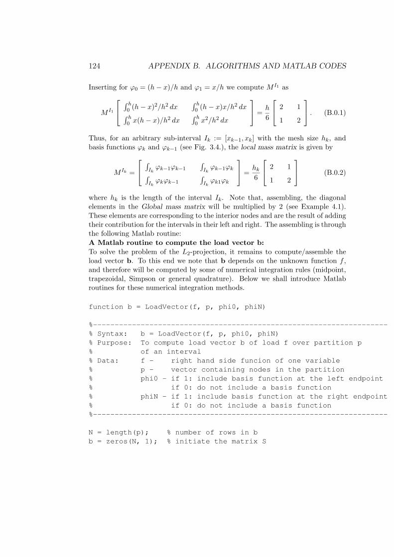
124 APPENDIX B. ALGORITHMS AND MATLAB CODES
Inserting for ϕ0 = (h− x)/h and ϕ1 = x/h we compute M I1 as
M I1
∫ h0 (h− x)2/h2 dx
∫ h0 (h− x)x/h2 dx
∫ h0 x(h− x)/h2 dx
∫ h0 x2/h2 dx
=
h
6
2 1
1 2
. (B.0.1)
Thus, for an arbitrary sub-interval Ik := [xk−1, xk] with the mesh size hk, andbasis functions ϕk and ϕk−1 (see Fig. 3.4.), the local mass matrix is given by
M Ik =
∫Ikϕk−1ϕk−1
∫Ikϕk−1ϕk
∫Ikϕkϕk−1
∫Ikϕk1ϕk
=
hk6
2 1
1 2
(B.0.2)
where hk is the length of the interval Ik. Note that, assembling, the diagonalelements in the Global mass matrix will be multiplied by 2 (see Example 4.1).These elements are corresponding to the interior nodes and are the result of addingtheir contribution for the intervals in their left and right. The assembling is throughthe following Matlab routine:
A Matlab routine to compute the load vector b:
To solve the problem of the L2-projection, it remains to compute/assemble theload vector b. To this end we note that b depends on the unknown function f ,and therefore will be computed by some of numerical integration rules (midpoint,trapezoidal, Simpson or general quadrature). Below we shall introduce Matlabroutines for these numerical integration methods.
function b = LoadVector(f, p, phi0, phiN)
%--------------------------------------------------------------------
% Syntax: b = LoadVector(f, p, phi0, phiN)
% Purpose: To compute load vector b of load f over partition p
% of an interval
% Data: f - right hand side funcion of one variable
% p - vector containing nodes in the partition
% phi0 - if 1: include basis function at the left endpoint
% if 0: do not include a basis function
% phiN - if 1: include basis function at the right endpoint
% if 0: do not include a basis function
%--------------------------------------------------------------------
N = length(p); % number of rows in b
b = zeros(N, 1); % initiate the matrix S

125
% Assemble the load vector (including basis functions at both endpoints)
for i = 1:length(p)-1
h = p(i + 1) - p(i); % length of the current interval
b(i) = b(i) + .5*h*f(p(i));
b(i + 1) = b(i + 1) + .5*h*f(p(i + 1));
end
% Remove unnecessary elements for basis functions not included
if ˜phi0
b = b(2:end);
end
if ˜phiN
b = b(1:end-1);
end
The data function f can be either inserted as f=@(x) followed by some ex-pression in the variable x, or more systematically through a separate routine, herecalled “Myfunction” as in the following example
Example B.1 (Calling a data function f(x) = x2 of the load vector).function y= Myfunction (p)
y=x.ˆ2
\vskip 0.3cm
Then, we assemble the corresponding load vector, viz:
\beginverbatim
b = LoadVector (@Myfunction, p, 1, 1)
Alternatively we may write
f=@(x)x.ˆ2
b = LoadVector(f, p, 1, 1)
Now we are prepared to write a Matlab routine “My1DL2Projection” for com-
puting the L2-projection.
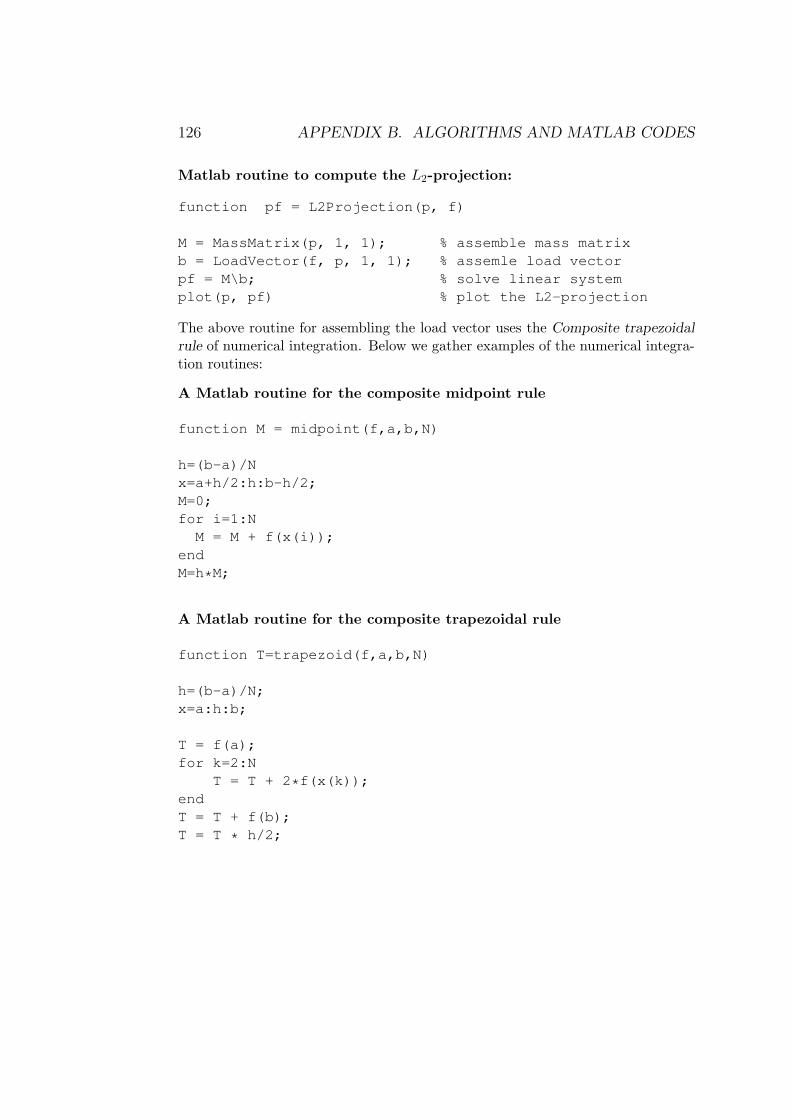
126 APPENDIX B. ALGORITHMS AND MATLAB CODES
Matlab routine to compute the L2-projection:
function pf = L2Projection(p, f)
M = MassMatrix(p, 1, 1); % assemble mass matrix
b = LoadVector(f, p, 1, 1); % assemle load vector
pf = M\b; % solve linear system
plot(p, pf) % plot the L2-projection
The above routine for assembling the load vector uses the Composite trapezoidal
rule of numerical integration. Below we gather examples of the numerical integra-tion routines:
A Matlab routine for the composite midpoint rule
function M = midpoint(f,a,b,N)
h=(b-a)/N
x=a+h/2:h:b-h/2;
M=0;
for i=1:N
M = M + f(x(i));
end
M=h*M;
A Matlab routine for the composite trapezoidal rule
function T=trapezoid(f,a,b,N)
h=(b-a)/N;
x=a:h:b;
T = f(a);
for k=2:N
T = T + 2*f(x(k));
end
T = T + f(b);
T = T * h/2;

127
A Matlab routine for the composite Simpson’s rule
function S = simpson(a,b,N,f)
h=(b-a)/(2*N);
x = a:h:b;
p = 0;
q = 0;
for i = 2:2:2*N % Define the terms to be multiplied by 4
p = p + f(x(i));
end
for i = 3:2:2*N-1 % Define the terms to be multiplied by 2
q = q + f(x(i));
end
S = (h/3)*(f(a) + 2*q + 4*p + f(b)); % Calculate final output
The precomputations for standard and local stiffness and convection matrices:
SI1 =
∫I1ϕ′0ϕ
′0
∫I1ϕ′0ϕ
′1
∫I1ϕ′1ϕ
′0
∫I1ϕ1′ϕ′
1
=
∫I1
−1h
−1h
∫I1
−1h
1h∫
I11h−1h
∫I1
1h1h
=
1
h
1 −1
−1 1
.
As in the assembling of the mass-matrix, even here, for the global stiffness matrix,each interior node has contributions from both intervals that the node belongs.Consequently, assembling we have 2/h as the interior diagonal elements in thestiffness matrix (rather than 1/h in the single interval computes above). For theconvection matrix C, however, because of the skew-symmetry the contributionsfrom the two adjacent interior intervals will cancel out:
CI1 =
∫I1ϕ′0ϕ0
∫I1ϕ0ϕ
′1
∫I1ϕ1ϕ
′0
∫I1ϕ1′ϕ1
=
∫I1
−1h
h−xh
∫I1
h−xh
1h∫
I1xh−1h
∫I1
xh1h
=1
2
−1 1
−1 1
.
A thorough computation of all matrix elements, for both interior and bound-ary nodes, in the case of continuous piece-wise linear approximation, for Mass-,stiffness- and convection-matrices are demonstrated in Examples 4.1 and 4.2.

128 APPENDIX B. ALGORITHMS AND MATLAB CODES
A Matlab routine assembling the stiffness matrix:
function S = StiffnessMatrix(p, phi0, phiN)
%---------------------------------------------------------------------
% Syntax: S = StiffnessMatrix(p, phi0, phiN)
% Purpose: To compute the stiffness matrix S of a partition p of an
% interval
% Data: p - vector containing nodes in the partition
% phi0 - if 1: include basis function at the left endpoint
% if 0: do not include a basis function
% phiN - if 1: include basis function at the right endpoint
% if 0: do not include a basis function
%---------------------------------------------------------------------
N = length(p); % number of rows and columns in S
S = zeros(N, N); % initiate the matrix S
% Assemble the full matrix (including basis functions at endpoints)
for i = 1:length(p)-1
h = p(i + 1) - p(i); % length of the current interval
S(i, i) = S(i, i) + 1/h;
S(i, i + 1) = S(i, i + 1) - 1/h;
S(i + 1, i) = S(i + 1, i) - 1/h;
S(i + 1, i + 1) = S(i + 1, i + 1) + 1/h;
end
% Remove unnecessary elements for basis functions not included
if ˜phi0
S = S(2:end, 2:end);
end
if ˜phiN
S = S(1:end-1, 1:end-1);
end
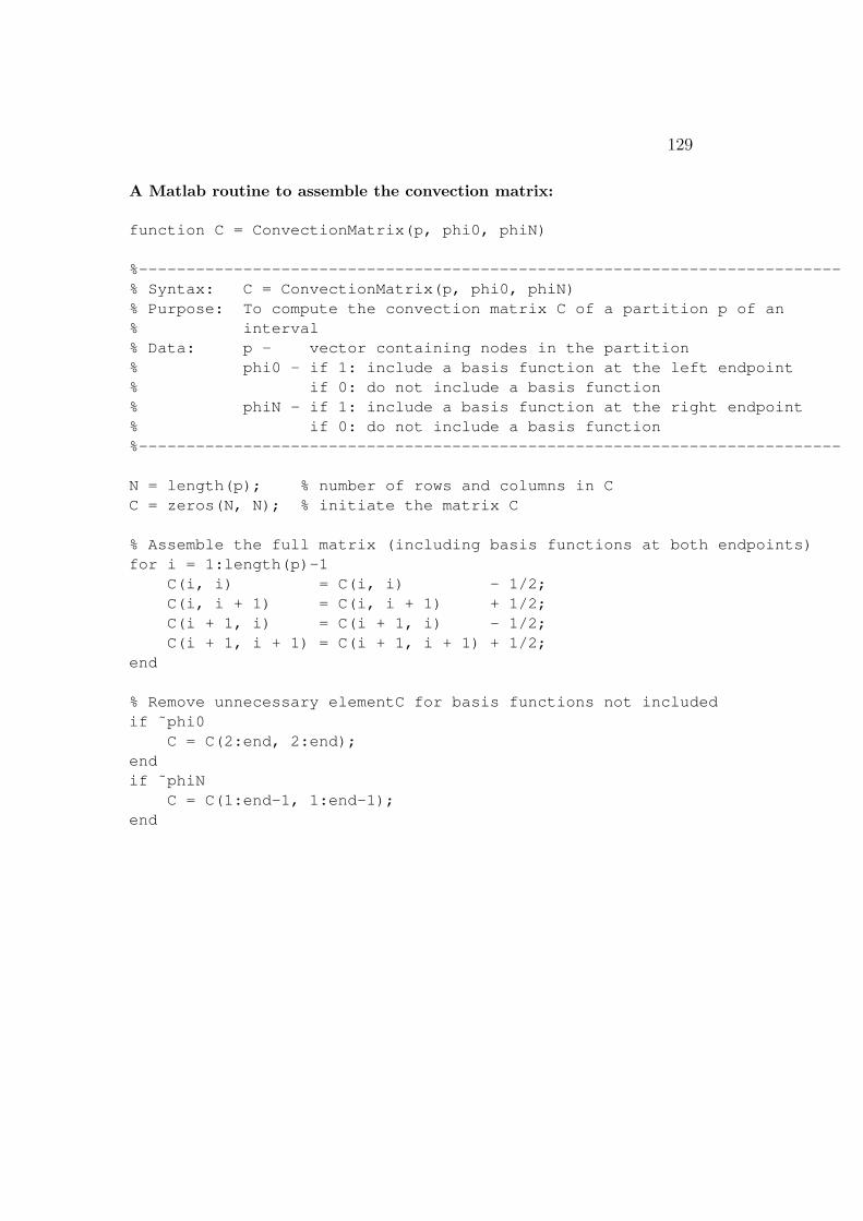
129
A Matlab routine to assemble the convection matrix:
function C = ConvectionMatrix(p, phi0, phiN)
%--------------------------------------------------------------------------
% Syntax: C = ConvectionMatrix(p, phi0, phiN)
% Purpose: To compute the convection matrix C of a partition p of an
% interval
% Data: p - vector containing nodes in the partition
% phi0 - if 1: include a basis function at the left endpoint
% if 0: do not include a basis function
% phiN - if 1: include a basis function at the right endpoint
% if 0: do not include a basis function
%--------------------------------------------------------------------------
N = length(p); % number of rows and columns in C
C = zeros(N, N); % initiate the matrix C
% Assemble the full matrix (including basis functions at both endpoints)
for i = 1:length(p)-1
C(i, i) = C(i, i) - 1/2;
C(i, i + 1) = C(i, i + 1) + 1/2;
C(i + 1, i) = C(i + 1, i) - 1/2;
C(i + 1, i + 1) = C(i + 1, i + 1) + 1/2;
end
% Remove unnecessary elementC for basis functions not included
if ˜phi0
C = C(2:end, 2:end);
end
if ˜phiN
C = C(1:end-1, 1:end-1);
end

130 APPENDIX B. ALGORITHMS AND MATLAB CODES
Finally, below we gather the Matlab routines for finite difference approxima-tions (also cG(1) and dG(0) ) for the time discretizations.
Matlab routine for Forward-, Backward-Euler and Crank-Nicolson:
function [] = three_methods(u0, T, dt, a, f, exactexists, u)
% Solves the equation du/dt + a(t)*u = f(t)
% u0: initial value; T: final time; dt: time step size
% exactexists = 1 <=> exact solution is known
% exactexists = 0 <=> exact solution is unknown
timevector = [0]; % we build up a vector of
% the discrete time levels
U_explicit_E = [u0]; % vector which will contain the
% solution obtained using "Forward Euler"
U_implicit_E = [u0]; % vector which will contain the
% solution with "Backward Euler"
U_CN = [u0]; % vector which will contain the
% solution using "Crank-Nicolson"
n = 1; % current time interval
t_l = 0; % left end point of the current
% time interval, i.e. t_n-1
while t_l < T
t_r = n*dt; % right end point of the current
% time interval, i.e. t_n
% Forward Euler:
U_v = U_explicit_E(n); % U_v = U_n-1
U_h = (1-dt*a(t_l))*U_v+dt*f(t_l); % U_h = U_n;
U_explicit_E(n+1) = U_h;
% Backward Euler:
U_v = U_implicit_E(n); % U_v = U_n-1
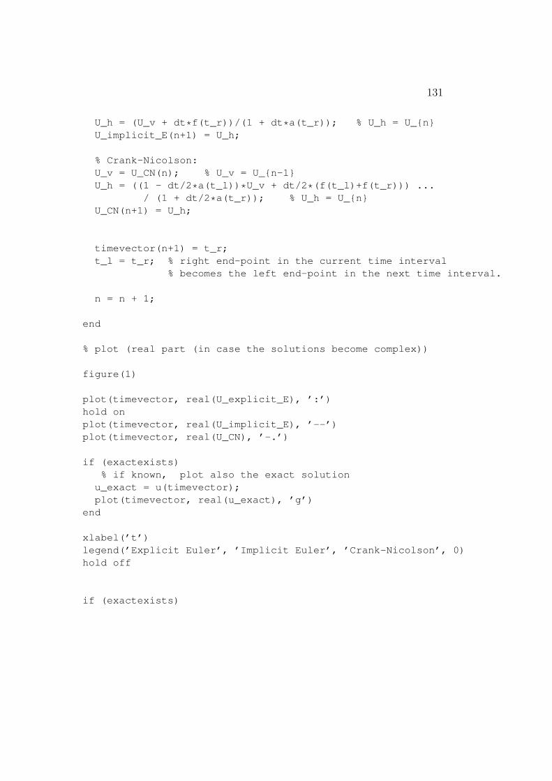
131
U_h = (U_v + dt*f(t_r))/(1 + dt*a(t_r)); % U_h = U_n
U_implicit_E(n+1) = U_h;
% Crank-Nicolson:
U_v = U_CN(n); % U_v = U_n-1
U_h = ((1 - dt/2*a(t_l))*U_v + dt/2*(f(t_l)+f(t_r))) ...
/ (1 + dt/2*a(t_r)); % U_h = U_n
U_CN(n+1) = U_h;
timevector(n+1) = t_r;
t_l = t_r; % right end-point in the current time interval
% becomes the left end-point in the next time interval.
n = n + 1;
end
% plot (real part (in case the solutions become complex))
figure(1)
plot(timevector, real(U_explicit_E), ’:’)
hold on
plot(timevector, real(U_implicit_E), ’--’)
plot(timevector, real(U_CN), ’-.’)
if (exactexists)
% if known, plot also the exact solution
u_exact = u(timevector);
plot(timevector, real(u_exact), ’g’)
end
xlabel(’t’)
legend(’Explicit Euler’, ’Implicit Euler’, ’Crank-Nicolson’, 0)
hold off
if (exactexists)
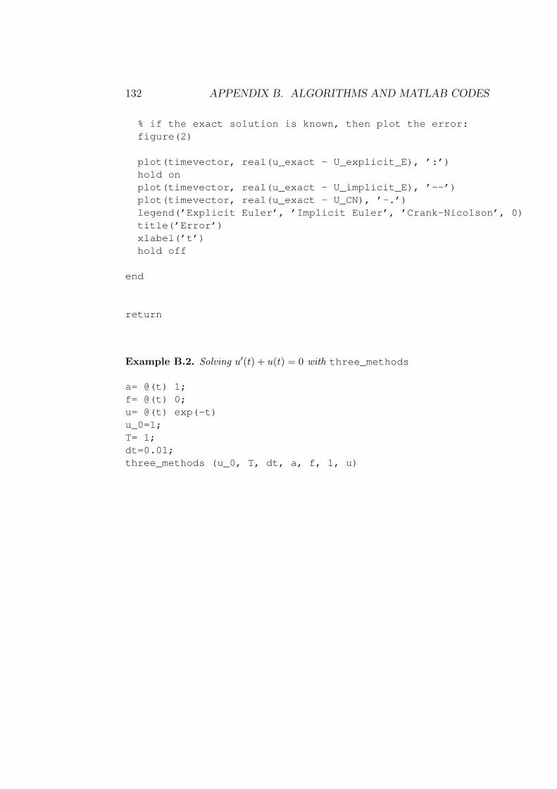
132 APPENDIX B. ALGORITHMS AND MATLAB CODES
% if the exact solution is known, then plot the error:
figure(2)
plot(timevector, real(u_exact - U_explicit_E), ’:’)
hold on
plot(timevector, real(u_exact - U_implicit_E), ’--’)
plot(timevector, real(u_exact - U_CN), ’-.’)
legend(’Explicit Euler’, ’Implicit Euler’, ’Crank-Nicolson’, 0)
title(’Error’)
xlabel(’t’)
hold off
end
return
Example B.2. Solving u′(t) + u(t) = 0 with three_methods
a= @(t) 1;
f= @(t) 0;
u= @(t) exp(-t)
u_0=1;
T= 1;
dt=0.01;
three_methods (u_0, T, dt, a, f, 1, u)

133
Table of Symbols
Symbol reads Definition
∀ for all, for every ∀x, cos2 x+ sin2 x = 1
∃ There exists see below
: such that ∃x : x > 3
∨ or x ∨ y (x or y)
∧ or & and x ∧ y (x and y) also x & y
∈ belongs√2 ∈ R (
√2 is a real numbers R)
/∈ not belongs√2 /∈ Q (
√2 is not a rational number )
⊥ orthogonal to u ⊥ v (u and v are orthogonal)
:= defines as I :=
∫ b
a
f(x) dx (I defines as integralen in RHS)
=: defines
∫ b
a
f(x) dx =: I (The integral in LHS defines I)
≈ approximates A ≈ B (A approximates B) or A is approximately equal B.
=⇒ implies A =⇒ B (A implies B.)
⇐⇒ equivalent A⇐⇒ B (A is equivalent to B.)
ODE Ordinary Differential Equation
PDE Partial Differential Equation
IVP Initial Value Problem
BVP Boundary Value Problem
VF Variational Formulation
MP Minimization Problem
Pq(I) p ∈ Pq(I) p(x) is a polynomial of degree ≤ q for x ∈ I.
H1(I) v ∈ H1(I) if
∫ b
a
(v(x)2 + v′(x)2
)dx <∞, I = [a, b].
Vh(I) v ∈ Vh(I) the space of piecewise linear functions on a partition of I.
V 0h (I) v ∈ V 0
h (I) v ∈ Vh(I) and v is 0 at both or one of the boundary points.
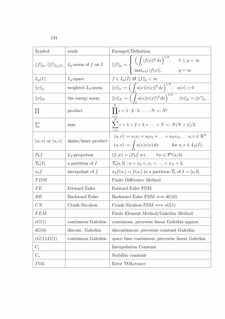
134
Symbol reads Exempel/Definition
||f ||p, ||f ||Lp(I) Lp-norm of f on I ||f ||p :=
(∫
I
|f(x)|p dx)1/p
, 1 ≤ p <∞
maxx∈I |f(x)|, p = ∞
Lp(I) Lp-space f ∈ Lp(I) iff ||f ||p <∞
||v||a weighted L2-norm ||v||a :=(∫
I
a(x)|v(x)|2 dx)1/2
, a(x) > 0
||v||E the energy norm ||v||E :=(∫
I
a(x)|v(x)′|2 dx)1/2
, ||v||E = ||v′||a.
∏product
N∏
i=1
i = 1 · 2 · 3 · . . . ·N =: N !
∑sum
N∑
i=1
i = 1 + 2 + 3 + . . .+N =: N(N + 1)/2
(u, v) or 〈u, v〉 skalar/inner product(u, v) := u1v1 + u2v2 + . . .+ uNvN , u, v ∈ RN
(u, v) :=
∫
I
u(x)v(x) dx for u, v ∈ L2(I).
Phf L2-projection (f, w) = (Phf, w), ∀w ∈ Pq(a, b).
Th(I) a partition of I Th[a, b] : a = x0 < x1 < . . . < xN = b.
πhf interpolant of f πhf(xi) = f(xi) in a partition Th of I = [a, b].
FDM Finite Difference Method
FE Forward Euler Forward Euler FDM
BE Backward Euler Backward Euler FDM ⇐⇒ dG(0)
CN Crank-Nicolson Crank-Nicolson FDM ⇐⇒ cG(1)
FEM Finite Element Method/Galerkin Method
cG(1) continuous Galerkin continuous, piecewise linear Galerkin approx
dG(0) discont. Galerkin discontinuous, piecewise constant Galerkin
cG(1)cG(1) continuous Galerkin space time continuous, piecewise linear Galerkin
Ci Interpolation Constant
Cs Stability constant
TOL Error TOLerance
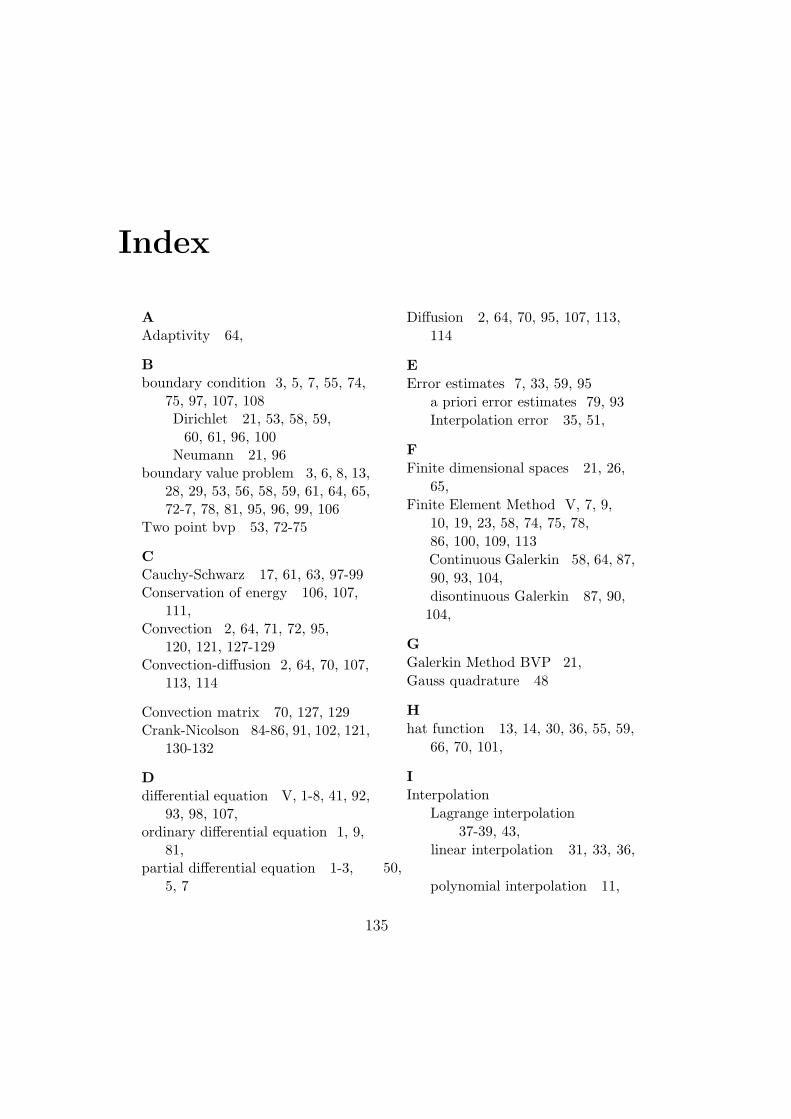
Index
AAdaptivity 64,
Bboundary condition 3, 5, 7, 55, 74,
75, 97, 107, 108Dirichlet 21, 53, 58, 59,60, 61, 96, 100
Neumann 21, 96boundary value problem 3, 6, 8, 13,
28, 29, 53, 56, 58, 59, 61, 64, 65,72-7, 78, 81, 95, 96, 99, 106
Two point bvp 53, 72-75
CCauchy-Schwarz 17, 61, 63, 97-99Conservation of energy 106, 107,
111,Convection 2, 64, 71, 72, 95,
120, 121, 127-129Convection-diffusion 2, 64, 70, 107,
113, 114
Convection matrix 70, 127, 129Crank-Nicolson 84-86, 91, 102, 121,
130-132
Ddifferential equation V, 1-8, 41, 92,
93, 98, 107,ordinary differential equation 1, 9,
81,partial differential equation 1-3,
5, 7
Diffusion 2, 64, 70, 95, 107, 113,
114
E
Error estimates 7, 33, 59, 95
a priori error estimates 79, 93
Interpolation error 35, 51,
F
Finite dimensional spaces 21, 26,
65,
Finite Element Method V, 7, 9,
10, 19, 23, 58, 74, 75, 78,
86, 100, 109, 113
Continuous Galerkin 58, 64, 87,
90, 93, 104,
disontinuous Galerkin 87, 90,
104,
G
Galerkin Method BVP 21,
Gauss quadrature 48
H
hat function 13, 14, 30, 36, 55, 59,
66, 70, 101,
I
Interpolation
Lagrange interpolation
37-39, 43,
linear interpolation 31, 33, 36,50,
polynomial interpolation 11,
135

136
Initial Boundary Value Problem
(IBVP) 3, 81, 95, 96, 99, 106,
Initial value problem 2, 3, 9, 17, 81,
(IBVP) 85-87, 92, 93
J, K
L
Lagrange basis 34,38-41, 50,
linear space 10, 15,
L2-projection 20, 21, 23, 121, 122,
124-126
M
Mass Matrix 67, 69, 102-104,
122-124, 126, 127
Minimization problem 53, 56, 57,
73,
Mixed bvp 96,
N
Neumann problem/data 21, 96,
Numerical integration 7, 31, 41, 121,
124, 126,
Composite midpoint 45
Composite trapezoidal 45
Composite Simpson’s 46
Simple midpoint 41, 45, 47
Simple trapezoidal 42, 45, 47,
85
Simple Simpson’s 43, 46, 48
Norm 16
L2-norm 16, 17, 63, 72, 97, 104,
105, 113, 114
Lp-norm 33, 35
vector norm 33
maximum norm 33, 35
energy norm 59, 60, 62, 75, 79
O
Ordinary Differential Equations
(ODE) 1, 7, 9, 28, 81 , 92Orthogonality 16, 29, 30, 59, 60
PPartial Differential Equations
(PDE) 1-3, 7, 10, 53, 65, 70, 98,107,heat equation 2, 21, 64, 95, 99,100, 105, 106, 108,wave equation 2, 3, 81, 95, 106,107, 111, 112
partition 10, 12-14, 20, 21, 26, 36,37, 39, 41, 44, 51, 58, 61, 64,65, 70, 73-75, 77-79, 83-85.
Poincare inequality 97-100, 105
Q
RResidual 18, 29, 30, 59, 61-64, 93
SScalar initial value problem, 81Scalar product 16, 17, 32, 33, 39stability 81, 82, 91, 93, 95-97, 99,
105, 115Stiffness matrix, 23-26, 28, 67, 71,
75, 92, 103, 127, 128
Ttest function 17-19, 21, 22, 54, 55,
58, 65, 70, 73, 87, 117trial function 18, 21, 65, 70, 87,
U
V/WVariational formulation 17, 22, 53.
XYZ


![[FEM] Geotechnical Analysis by the Finite Element Method](https://static.fdocuments.in/doc/165x107/55cf9734550346d033903ce5/fem-geotechnical-analysis-by-the-finite-element-method.jpg)


