Apphed Acousttcs 14 (1981) 455~169

AN INTRODUCTION TO STATISTICAL ENERGY ANALYSIS OF STRUCTURAL VIBRATION

J WOODHOUSE

Topexpress Ltd, 1 Portugal Place, Cambridge CB5 8A F (Great Britain)

(Recetved 22 February. 1981)

SUMMARY

The ideas of the approach to vlbratton analysts called Stattsttcal Energy Analysts (SEA) are e~plored wtthout going mto great techmcal detad The arm oj thts descrtptlon zs to gwe gutdance to those with parttcular vtbtatton problems who may ask whether the), should be using SEA and, t f so, what expectattons they should have o f tt In the fivst sectton, SEA in its most common fo rm ts tllustrated by the stmplest example

In the second sectton, the questton o f the underlying assumptions o f SEA is considered by a stmple and appatentl), novel approach Thts dtscusston also gives some mfol matlon on posstble methods o f measurmg the SEA parameter~ tn a gtven ptoblem and decldmg whetheJ a SEA model ts indeed appt oprtate for that problem We also attempt to gtve gutdance on how SEA should be apphed to a gtven problem, especially how the system under study should be dtvtded up into subsystems

One area m whtch SEA can be espectally useful ts m the destgn o f a systematw sequence o f expet iments on ful l ot model scale when tD'lng to pm down the source o f a pat tlculat vtbratlon ptoblem SEA can provide a successton of models, starting wtth the stmpleat possible and becommg ptogresstvelv mote comphcated, whwh enable results to be mtetpteted and suttable questtom to be asked Jot the new stage oJ testmg Thta ts a mote valuable set vtce than ts commonly applectated without such guMance, an e~pet lmentet faced wtth a ~ omphcated stt uctut e can ~pend a vet v long ttme makmg measurements ~htch turn out not to address the problem m hand

INTRODUCTION

Analysis of the vibratory behavlour of a complex structure can be under taken m two basically different ways If one ~s interested m gross movements of the structure on a

455 Apphed Acoustws 0003-682X/81/0014-0455/$02 50 © Apphed Science Pubhshers Ltd, England, 1981 Printed m Great Britain

456 J WOODHOUSE

large scale--for example, to study the flexing of a ship's hull m a heavy sea--then detailed study of the lowest frequency vibration modes is appropriate A great deal is known about such analysis, largely as a result of the monumental work of Lord Raylelgh at the end of the last century 1 Indeed, theory has not advanced much since Raylelgh's day although the spectacular development of computing power m recent

years has made brute-force numerical calculation of such modal behavlour in complex structures feasible for the first time (the finite element method, NASTRAN, etc )

If, on the other hand, the main interest is m the behaviour of the structure at higher frequencies, deterministic analysis of individual modes becomes less feasible and also less useful There are four reasons for this First, the modes crowd together in frequency so that many more of them need to be considered Secondly, higher frequency (l e shorter length-scale) modes are more sensitive to the inevitable small variations in structural detail even in nominally identical structures, so that they are harder to predict reliably Thirdly, related to the previous point, numerical accuracy decreases as one goes higher up the mode series so that, even if the real structure behaves like the model under study, the numerical predictions from the model may not be reliable Finally, even if an accurate and relevant numerical simulation can be made in the high frequency range under discussion there is the problem that computer output tends to be voluminous to the point of indigestibility when the model is complicated, so that it is hard to make use of the results In particular, for a model with many parameters, one needs some estimate of the sensitivity of the predictions to variations in all these parameters since they will be known only approximately for the real structure Usually the only way this is attempted in a numerical study is by changing each parameter in turn and running the program again, and it is clear that the more parameters there are, the more the problem of indigestibility of the results is multiplied

In the face of all these difficulties it is frequently more appropriate to use statistical techniques to average out in a suitable way the detailed modal behaviour one can then discuss such ideas as mean power flow between parts of the structure in a given frequency band or the expected spatial distribution of vibrational energy in the structure when broad band input is supplied at a locahsed place--for example, from an engine

The two approaches to the problem, deterministic and statistical, are not in competition for the great majority of applications statistical techniques take over from deterministic techniques, both in feasibility and usefulness, as the frequency range of interest rises through the mode series of the structure With the determlmstlc approach, as we have just said, computation of individual modal behavlour becomes increasingly difficult and unreliable as we go to higher mode numbers (beyond twenty or thirty, perhaps) The statistical approach, on the other hand does not require such detailed calculations and becomes increasingly

INTRODUCTION TO STATISTICAL ENERGY ANALYSIS 457

successful as the resonance frequency spacing gets smaller (compared with the half- power bandwidth of each mode) the more modes one can average over, the more reliable the average becomes as an estimate of what actually happens in the structure There may be an mtermedaate frequency range where both approaches can be tried, but in such a s~tuatlon ~t is possible that neither method wdl give entirely satisfactory results

The statlst~cal method IS paramount m architectural a c o u s t i c s , 2 s i n c e the number of modes of a large audltormm within the audible frequency range run Into tens of mdllons In such a situation one can expect statistics to be very rehable, whde deterministic methods are obviously out of the question We cannot expect structural problems to present quite so many modes to work on, so, whde the architectural acoust~cmn can use statistical methods without a second thought, m structural problems we must take care m each situation to assess the expected rehabfllty of our estimates Work is stdl m progress to enable this to be done more rehably than at present, but we do not dlscuss this here since our primary aim is to give a useful overwew of the staUstlcal approach, especmlly the particular techmque known as SEA

THE STATISTICAL ENERGY METHOD AND ITS THERMAL ANALOGY

Having seen that for many practical problems deterministic analysis is not useful and statistical analysis must be used, we now discuss what kind of results a statistical analysis will give We discuss primarily the existing body of methods and results known as SEA, 3 but we should note that this represents only a particular class of possible techniques which are, in some sense, statistical Extensions and generahsat~ons of conventional SEA to widen its scope of applicability are being developed in various places at present The recent review by Skudrzyk 4 IS an example of a somewhat different statistical approach from the one we discuss here

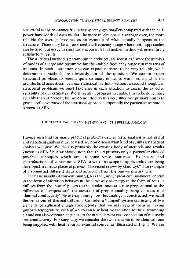
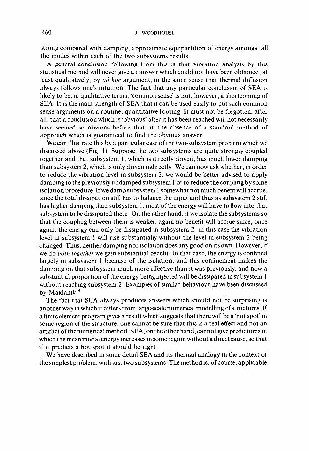
The basic insight of conventional SEA is that, under most circumstances, energy m the form of v~brat~on behaves m the same way as energy m the form of heat ~t diffuses from the 'hotter' places to the 'cooler' ones at a rate proportional to the difference of 'temperature', the constant of proportlonahty being a measure of 'thermal conductlwty' Before explaining how this analogy ~s constructed, we recall the behawour of thermal diffusion Consider a ' lumped' system consisting of two elements of sufficiently high conduct~wty that we may regard them as hawng umform temperature, each of which can lose heat by radlat~on to the surrounding mr and can also commumcate heat to the other element vm a connection of relatively low conductivity For s~mphc~ty we consider the two elements to be Identical, one being supphed w~th heat from an external source, as illustrated m F~g 1 We are

4 5 8 J WOODHOUSE

/2 /2

Fig 1 The simplest example of thermal diffusion, which dlustrates the thermal analogue of SEA Two ldent~cal thermally conducting elements are connected by a hnk with lower conductwlty Each element can also lose heat by ra&atlon to the surroundmgs and one element ~s heated by an external source

COUPLING

h~gh

Low

RADIATION

high

(al ]- (c)

[0w

1-- (b)

d)

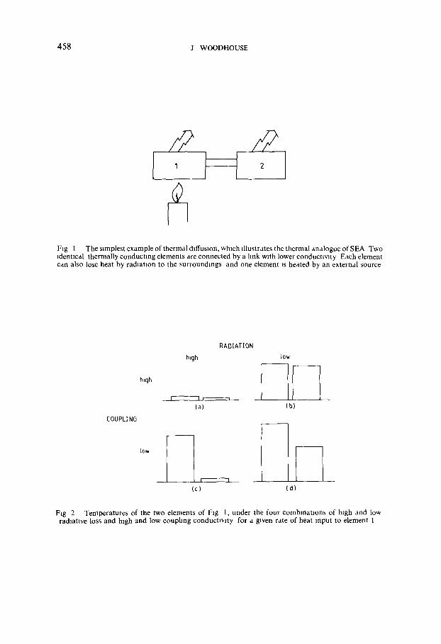
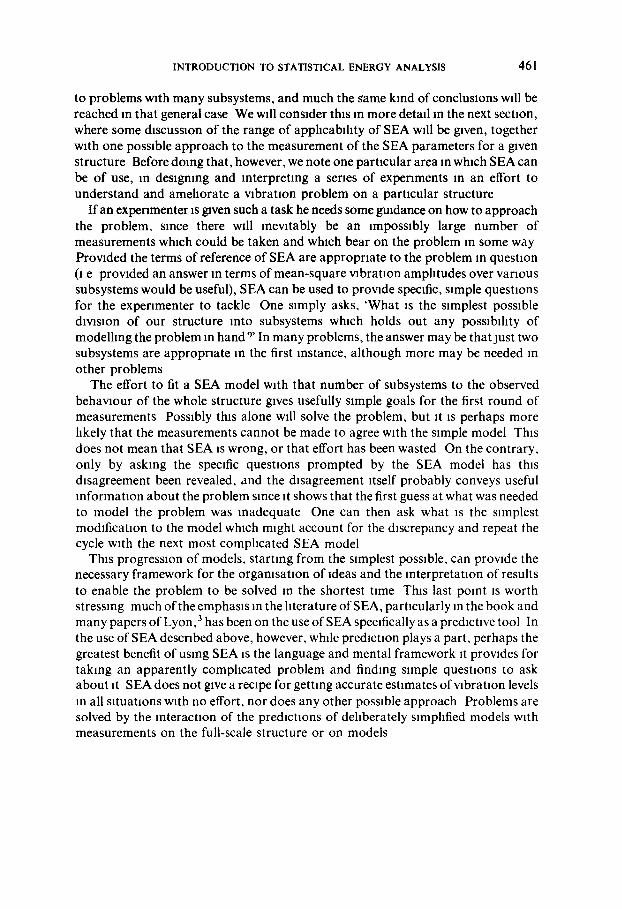
Ftg 2 Temperatures of the two elements of Fig 1, under the four combmatlon~ of high and low ra&atwe loss and high and low couphng conductwlty for a gwen rate of heat input to element 1

INTRODUCTION TO STATISTICAL ENERGY ANALYSIS 459

interested in the equilibrium temperatures In the two elements which result, under the various condmons of high and low radiation loss and high and low coupling conductivity

These temperatures are illustrated in Fig 2 Notice that cases (a) and (d) give the same ratio of temperatures between the two elements, since this depends only on the ratio of radiative loss to coupling conductivity, which is the same in both cases The absolute magmtudes of temperatures are greater in case (d), of course, since, for a given rate of heat input, both elements must get hotter to compensate for the smaller value of radiative loss factor In case (b), the couphng is so strong compared with the radmtlve loss that the two elements are not really separate and both have approximately the same temperature (that is, we have approximate equtpartttton of energy between elements) In case (c), radiation IS so much more effective than coupling between the elements that element 2 hardly knows that element 1 is being heated since the heat input ~s almost entirely balanced by radiation from element 1

To relate this thermal model to structural wbrat~on, we consider a complex structure which consists of two coupled substructures These might, for example, be two plates separated by a stiffening beam, or the hull and one deck of a vessel Now, prowded our substructures have an adequate number of modes w~thln the frequency range m which we are interested, we can average over these modes and regard the mean modal energy m each substructure In that frequency range as a measure of the ' temperature ' of the substructure We can then ~dentify the parameters of the mechamcal system with those of the thermal system as follows

(1) Thermal capacity of the element corresponds to modal denstty, that is, the number of modes whose frequencies fall within a gwen range

(n) Radmtlve loss corresponds to damping of the vibration modes m that frequency range

(111) Conductwlty, or loss by coupling, corresponds to a measure of the strength of the mechanical coupling of the substructures (derived, for example, from relative impedance)

With these identifications, flow of wbratlonal energy m the structure behaves m the same easily wsuahsed way as flow of heat m the thermal analogy

Thus we can now regard the four cases of Fig 2 as showing how the mean-square vibration level in the two substructures depends on the strengths of damping loss and couphng loss The source of heat in Fig 1 becomes a source of vibration, such as a machine attached to subsystem 1 We have, therefore, a very simple way of d~scussmg the effect on vlbrat~on tn subsystem 2 of changing the damping m either subsystem, or of isolating the two subsystems we can regard the at tempt to mlnlmlse vibration level m subsystem 2 as the prototype for all noise and vibration control problems The description in wbratlon terms of the four cases of Fig 2 parallels the description gwen above In thermal terms for example, when couphng is

460 J WOODHOUSE

strong compared with damping, approxamate equlpartltlon of energy amongst all the modes within each of the two subsystems results

A general conclusion following from this is that vibration analysis by this statastlcal method wall never gave an answer whach could not have been obtained, at least qualitatively, by ad hoc argument, an the same sense that thermal diffusion always follows one's mtuitaon The fact that any particular conclusaon of SEA as hkely to be, in quahtative terms, 'common sense' as not, however, a shortcoming of SEA It is the mare strength of SEA that at can be used easily to put such common sense arguments on a routine, quantitative footing It must not be forgotten, after all, that a conclusion which is 'obvious' after at has been reached wall not necessardy have seemed so obvaous before that, an the absence of a standard method of approach which is guaranteed to find the obvaous answer

We can illustrate thas by a partacular case of the two-subsystem problem whach we discussed above (Fig 1) Suppose the two subsystems are quate strongly coupled together and that subsystem 1, which is directly driven, has much lower damping than subsystem 2, whach is only driven Indirectly We can now ask whether, an order to reduce the vibration level an subsystem 2, we would be better advised to apply damping to the previously undamped subsystem I or to reduce the couphng by some isolation procedure If we damp subsystem 1 somewhat not much benefit will accrue, since the total dassapatlon stall has to balance the input and thus as subsystem 2 stdl has hagher damping than subsystem 1, most of the energy will have to flow into that subsystem to be &ss~pated there On the other hand, ffwe ~solate the subsystems so that the couphng between them is weaker, again no benefit wall accrue since, once again, the energy can only be dasslpated m subsystem 2 an thas case the wbratmn level in subsystem 1 will nse substantmlly without the level m subsystem 2 being changed Thus, neither damping nor isolation does any good on ats own However, af we do both together we gain substantial benefit In that case, the energy is confined largely an subsystem 1 because of the asolataon, and thas confinement makes the damping on that subsystem much more effectwe than it was prevaously, and now a substantial proportaon of the energy being rejected will be d~ssipated an subsystem 1 without reaching subsystem 2 Examples of samflar behawour have been &scussed by Maadamk 5

The fact that SEA always produces answers which should not be surprising is another way m whach at differs from large-scale numerical modelhng of structures If a fimte element program gives a result which suggests that there will be a 'hot spot' an some region of the structure, one cannot be sure that this xs a real effect and not an artifact of the numeracal method SEA, on the other hand, cannot gave predictions m which the mean modal energy increases m some regaon without a &rect cause, so that if it predacts a hot spot it should be right

We have described in some detail SEA and its thermal analogy m the context of the samlalest problem, with lust two subsystems The method ~s, of course, apphcable

INTRODUCTION TO STATISTICAL ENERGY ANALYSIS 461

to problems with many subsystems, and much the game kind of conclusions will be reached in that general case We will consider this in more detail In the next section, where some discussion of the range of applicability of SEA will be given, together with one possible approach to the measurement of the SEA parameters for a given structure Before doing that, however, we note one particular area in which SEA can be of use, In designing and Interpreting a series of experiments in an effort to understand and ameliorate a vibration problem on a particular structure

I f an experimenter is given such a task he needs some guidance on how to approach the problem, since there will inevitably be an impossibly large number of measurements which could be taken and which bear on the problem in some way Provided the terms of reference of SEA are appropriate to the problem in question (i e provided an answer in terms of mean-square vibration amplitudes over various subsystems would be useful), SEA can be used to provide specific, simple questions for the experimenter to tackle One simply asks, 'What IS the simplest possible dlwslon of our structure into subsystems which holds out any possibility of modelling the problem in hand 9' In many problems, the answer may be that just two subsystems are appropriate in the first instance, although more may be needed in other problems

The effort to fit a SEA model with that number of subsystems to the observed behaviour of the whole structure gives usefully simple goals for the first round of measurements Possibly this alone will solve the problem, but it is perhaps more likely that the measurements cannot be made to agree with the simple model This does not mean that SEA is wrong, or that effort has been wasted On the contrary, only by asking the specific questions prompted by the SEA model has this disagreement been revealed, and the disagreement itself probably conveys useful information about the problem since it shows that the first guess at what was needed to model the problem was inadequate One can then ask what is the simplest modification to the model which might account for the discrepancy and repeat the cycle with the next most complicated SEA model

This progression of models, starting from the simplest possible, can provide the necessary framework for the organlsatlon of ideas and the interpretation of results to enable the problem to be solved in the shortest time This last point is worth stressing much of the emphasis in the literature of SEA, particularly In the book and many papers of Lyon, 3 has been on the use of SEA specifically as a predictive tool In the use of SEA described above, however, while prediction plays a part, perhaps the greatest benefit of using SEA is the language and mental framework it provides for taking an apparently complicated problem and finding simple questions to ask about it SEA does not give a recipe for getting accurate estimates of vibration levels in all situations with no effort, nor does any other possible approach Problems are solved by the interaction of the predictions of deliberately simplified models with measurements on the full-scale structure or on models

462 J WOODHOUSE

DETERMINATION OF SEA PARAMETERS BY THE INVERSE PROBLEM, AND TESTING THE

VALIDITY OF A SEA MODEL

Having described the terms of reference of a SEA model and gwen some impression of the sort of answer which it can be expected to gwe, we now examme the circumstances under which we expect a SEA model to be vahd We are also interested In how SEA parameters might be determmed In the exlstmg SEA hterature, 3 lncludmg the previous work of the present author,61the question of the apphcabdmty of SEA has generally been approached by first consldermg the power flow between Individual modes of subsystems, then makmg appropriate statistical approxlmat~ons to obtain statements about the average power flow between the subsystems In domg such calculations, a set o fcondmons sufficient tolguarantee~the validity of the SEA model is found, and these condmons are frequently very restnctwe Thus the impression is gwen that SEA is only valid under very hmlted conditions In what follows we give an account of this problem from a dtfferent point of view We think that this is both useful in itself and provides a counterweight to the other method since it shows that SEA is, in fact, valid under rather general circumstances

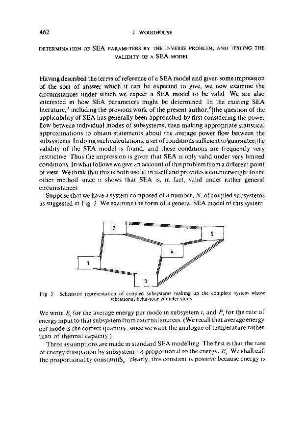
Suppose that we have a system composed of a number, N, of coupled subsystems as suggested in Fig 3 We examine the form of a general SEA model of this system

F~g 3

2

U--

Schematic representation of coupled subsystems makmg up the complete system whose vibrational behavlour is under study

We write E, for the average energy per mode in subsystem t, and P, for the rate of energy input to that subsystem from external sources (We recall that average energy per mode ~s the correct quantity, smce we want the analogue of temperature rather than of thermal capacity )

Three assumptions are made m standard SEA modelhng The first is that the rate of energy dissipation by subsystem ~ is proportional to the energy, E, We shall call the proportionality constantlS,, 'clearly, this constant is posltwe because energy is

I N T R O D U C T I O N TO STATISTICAL ENERGY ANALYSIS 463

being dissipated, not created The second assumption is that the rate of power flow from subsystem t to subsystemj is proport ional to the difference of their energies we take it to equal S , ~ ( E , - E ) Again, it is clear that the constants S,j are all non- negative (some may well be zero, of course, since some subsystems will not be directly coupled to others at all) The third assumption is that the driving forces on the different subsystems are statistically independent so that we can add the energy responses of a given subsystem produced by these different driving forces to obtain the total mean modal energy of that subsystem

Energy balance on subsystem t now requires that

S.E, + ~ S,j(E, - Ej) = P, (1)

where the sum over . / represents all energy flow away from subsystem 1 to other subsystems (Those who are familiar with electrical clrcmt theory will now be aware of an alternative analogue of SEA to the thermal one discussed above eqn (1) is a statement of Klrchhoff 's law )

Our eventual aim is to use the SEA model to predict the change in vibrational behavlour of the whole system when some modification is made to the structure To do this we need to know the energies, E,, in response to given rates of external energy input, P, At present, eqn (1) expresses the P,'s m terms of the E,'s, so we must Invert this relation To achieve this, we first rearrange eqn (1) by collecting all occurrences of each E, together, to read

N i,=====~

P, = ~' X,jE~ (2)

j = l

I ~- S,~ t 4:J (3)

X~---- k SLk l = J

1

We now invert the matrix of eqn (2) to obtain the desired form of predictions

N

E, = ~ ' A,jPj (4)

J = l

We have written A for the inverse of X we shall discuss below the physical Interpretation of matrix A

where

464 J WOODHOUSE

From th~s form of the SEA model of the system, we can note an ~mportant general point Since both matrices A and Xare symmetric, the model expressed by matrix X has precisely the same number of parameters as the number of predictions sought (although we should note that, m practice, with many subsystems, we expect some pa~rs of subsystems to have no direct couphng so that certain off-d~agonal elements of X will be zero), expressed in matrix A Th~s immediately suggests that the conditions of apphcablhty of the SEA model cannot be very restrlctwe, since we have so many adjustable parameters in our model Since the model is not substantially more compact than the predlcUons it yields, we must ask what benefit we derive from the SEA model why can we not proceed straight to the matrix A 9

The answer to this hes in the fact that we have a more direct and useful physical interpretation of the terms of X, since we can readily derive from them the terms of matrix S, of which the diagonal elements express the damping m the mdwidual subsystems, while the off-diagonal elements describe the strength of couphng between pairs of subsystems Thus, ffwe are using the SEA model to study how the wbranonal behawour of the whole system will change when some modification ~s made to the structure, we would expect to be able to describe that structural change in terms of one, or at most a few, elements of Xchanglng Having charactensed the change in X, we can then, of course, use the model to evaluate the change m .4 If we were trying to predict A directly, however, we would have to contend with the fact that any change in the structure will in general change all the elements of .4 Thus the SEA model can gwe useful insight into the sensitivity of the vibrational behawour of the system to such structural modifications

Having seen that the SEA model is worth having, we need to answer two questions--When ~s a SEA model vahd9 How do we evaluate the model parameters S~j 9 We approach these questions simultaneously by asking how one could determine experlmentall~ whether an SEA model is valid We imagine performing a set of measurements on this system, in which we drive one subsystem at a time, and measure the response of all the subsystems in each case Thus, if we drive subsystem i w~th a rate of energy input scaled to unity, we can determine the mean energy per mode in subsystem 1, which will be the matrix element A,j Thus, the matrix A is directly observable If, now, all the subsystems are driven simultaneously with the energy input rates, P,, provided we make the single assumption that the driving forces on the different subsystems are stansncally independent, we can superimpose these energy responses to obtain the total mean modal energy of subsystem l m the form of eqn (4)

Thus we expect the subsystem responses to depend on the inputs to the various subsystems in a simple matrix fashion under very general circumstances the question of the validity of the SEA model hinges on whether this matrix has the appropriate form of reverse to look like a SEA model as m eqn (3) The only constraints on the apphcabfl~ty of SEA to the system m quesnon lie m the stgns of the matrix entries 4 is composed entirely of non-negatwe terms, while X has all its off-

INTRODUCTION TO STATISTICAL ENERGY ANALYSIS 465

diagonal terms non-positive and all Its diagonal terms posltave and suffioently large that the sum along any row is non-negative A SEA model is thus valid for any system whose matrix A has an Inverse In the form X

To evaluate precisely the conditions on the matrix A which guarantee such an reverse would take us into research problems in linear algebra, beyond the scope of this introductory account We thus content ourselves here with two s~mple examples of these conditions, for the case of just two subsystems and for the case of very weakly coupled subsystems For the two-subsystem case, we suppose our matrax A has the form

where a, b and c are all posatlve numbers Then the inverse as

1 ' 5 ,6, where

A = ac - b z

Hence any such matrix A has an inverse whose diagonal terms are posmve and whose off-diagonal terms are negative provided that A > 0 Our other condition is that the sum of any row of the inverse matrix should be positive, and this requires

a > b c > b (7)

which as also sutficaent to ensure the con&tlon A > 0 Thus we find that for a system composed of just two subsystems, the only condition necessary for the validity of an SEA model in the terms formulated here is that m the observed matrix A, whenever one subsystem only is driven, that subsystem should respond with greater mean modal energy than the other, non-driven, subsystem This condition is physically very plausible and we can deduce that SEA should always be apphcable to any problem w~th just two subsystems

For the case of weakly coupled subsystems, the matrix A will have the diagonal element much larger than all the off-diagonal elements in each row, since the driven subsystem will always vibrate much more vigorously than the others We shall show that if th~s diagonal dominance is sufficiently strong, the inverse matrix will necessarily be in SEA form Write the matrix A as the sum of a diagonal matrix D and a matrix E whose diagonal elements are zero and all of whose off-diagonal elements are much smaller than a typical diagonal element of D Then first-order perturbation theory says that the inverse of A is given approximately by

A - 1 ~ - D - 1 - D - 1 E D - x (8)

which has the correct sign pattern for a SEA model and also satisfies the constraint of the sum of any row being non-negative provided the diagonal dominance of A was

466 J WOODHOUSE

sufficiently s t rong (1 e the coupl ing sufficiently weak) Thus sufficiently weak coupl ing, like the case of two subsystems, guarantees the correct form of inverse

mat r ix and thus the appl icab i l i ty o f a SEA mode l wi thout fur ther condi t ions Wi th many subsystems and s t ronger coupl ing, things are more compl ica ted and

we do no t discuss the p rob l em in detai l Re tu rn ing to our imagined exper iment on such a system, we can now enquire a little more closely how we should test our measured matr ix A to de te rmine whether a SEA model would be valid and, if so, how to de termine the SEA pa rame te r s We first evaluate A - 1 to find out whether it is in the form X If it is, all Is well If ,t is not , however, we do not necessari ly give up and conclude that SEA is not usable There will be errors In the measurements of A,j, so we must next ask whether we can find a modif ica t ion o f A within the error bands of the measurements which does have an inverse in the correct form Once we have found such an A, then all the SEA pa rame te r s are de te rmined since, f rom X, we can deduce S, which is composed of the d a m p i n g loss factors and coupl ing loss factors called for in the SEA model

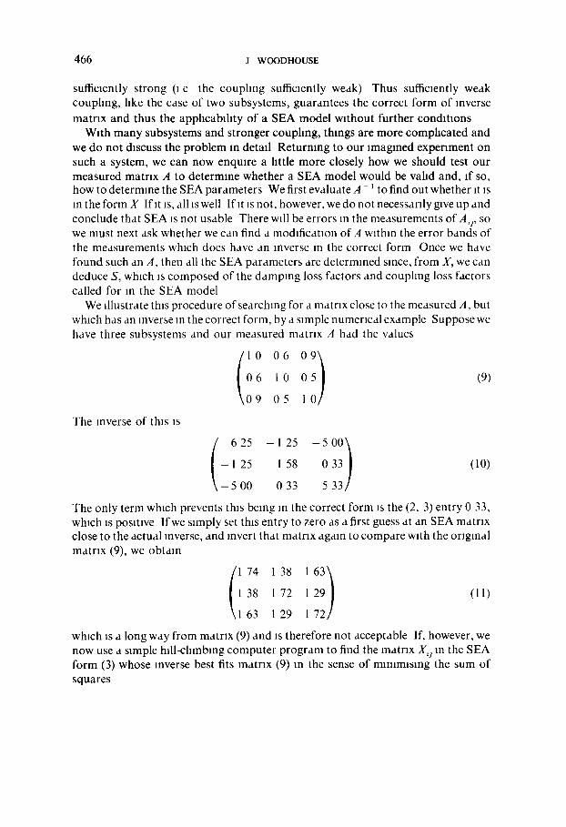
We i l lustrate this p rocedure of searching for a mat r ix close to the measured A, but which has an inverse m the correct form, by a simple numer ica l example Supposewe have three subsystems and our measured matr ix A had the values

0 6

6 l 0 0 (9)

9 0 5 1

The reverse o f this is

t 6 25 l 25 - 5 \ - 00

- l 25 1 58 0 3 3 ) (10)

- 5 00 0 33 5 33

The only term which prevents this being in the correct form is the (2, 3) entry 0 33, which is positive If we s imply set this en t ry to zero as a first guess at an SEA matr ix close to the ac tual inverse, and invert that mat r ix again to c ompa re with the or iginal mat r ix (9), we obta in (i 63) 1 74 l 38 1

38 l 72 l 29

63 1 29 1 72

(11)

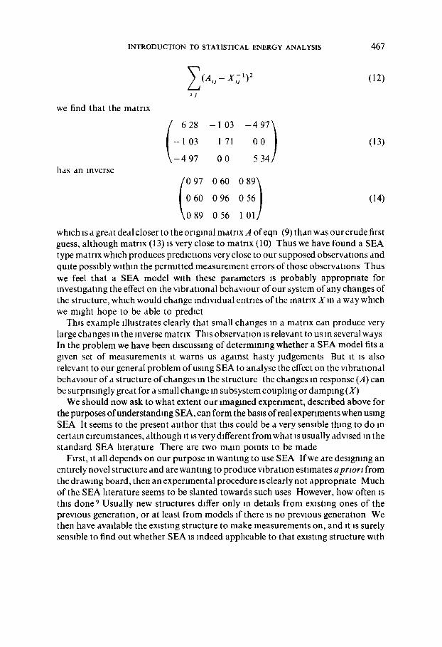
which is a long way from matr ix (9) and is therefore not acceptable If, however, we now use a simple hi l l -cl imbing c o m p u t e r p r o g r a m to find the matr ix X,j in the SEA form (3) whose inverse best fits mat r ix (9) in the sense o f manlmlslng the sum of squares

INTRODUCTION TO STATISTICAL ENERGY ANALYSIS 467

we find that the matrix

has an inverse

~ ( A , s - X ~ l ) 2

i j

(12)

_,03 _49;) 1 03 1 71 0

4 97 0 0 5 3 4 /

(13)

097 060 089 t

060 096 056 (14)

0 89 0 56 1 01

which is d great deal closer to the original matrix A ofeqn (9) than was our crude first guess, although matrix (13) is very close to matrix (10) Thus we have found a SEA type matrix which produces predictions very close to our supposed observations and qmte possxbly w~thm the permitted measurement errors of those observations Thus we feel that a SEA model w~th these parameters is probably appropriate for investigating the effect on the wbrat~onal behavlour of our system of any changes of the structure, which would change individual entraes of the matrix X in a way which we m~ght hope to be able to predict

This example illustrates clearly that small changes in a matrix can produce very large changes m the reverse matrix This observation ~s relevant to us in several ways In the problem we have been discussing of determining whether a SEA model fits a gwen set of measurements ~t warns us against hasty judgements But It is also relevant to our general problem of using SEA to analyse the effect on the wbrat~onal behavlour of a structure of changes m the structure the changes m response (A) can be surprisingly great for a small change m subsystem couphng or damping (X)

We should now ask to what extent our imagined experiment, described above for the purposes of understanding SEA, can form the basis of real experiments when using SEA It seems to the present author that th~s could be a very sensible thing to do m certain circumstances, although it is very d~fferent from what ~s usually advised in the standard SEA hterature There are two mare points to be made

First, it all depends on our purpose m wanting to use SEA If we are designing an entirely novel structure and are wanting to produce wbrat~on estimates apr~ort from the drawing board, then an experimental procedure ~s clearly not appropriate Much of the SEA hterature seems to be slanted towards such uses However, how often ~s th~s done9 Usually new structures d~ffer only m details from existing ones of the previous generation, or at least from models ff there is no prewous generation We then have available the existing structure to make measurements on, and it ~s surely sensible to find out whether SEA is indeed apphcable to that existing structure w~th

468 J WOODHOUSE

our chosen decomposition into subsystems before asking whether we can use SEA to study change~ in the structure'~ The method described above can do this reasonably easily Having done that, and in the process determined all the SEA model parameters for the existing structure, we are in a position to investigate the changes in those parameters resulting from our proposed structural changes, and thus to study the effect on vibrational response

This brings us to the second main point to be made much of the emphasis in the SEA literature is on ~al~ulatmg coupling loss factors--that IS, elements of S,j-- whereas here we are advocating measuring them all Does this not represent an unnecessardy large experimental effort ~ The answer is, if one studies the SEA literature closely, that for realistic structure-structure coupling problems, coupling loss factors are very hard to predict reliably on theoretical grounds, and one has to resort to measurement in any case (see especially the chapter in Lyon's book 3 on determining coupling loss [actors) If one is going to have to resort to measurement in any case, the author would suggest that the procedure described above could be simpler and more systematic, as well as more Informative, than the approaches suggested by Lyon and others

Having made the point that coupling loss factors have to be measured rather than calculated, we must now address the question of whether it is therefore impossible to predict the effect on the elements of X of changes in the structure Fortunately, th~s need not be the case While it may be very hard to predict these values aprtor~ with no experimental mformat~on, it can be very much easier to predict, at least to an acceptable approximation, the dependence of a given term on a particular parameter of the structure such as a plate thickness usually some power-law dependence can be deduced from simple modelling of the structure Thus, with the experimental determination of the coupling loss factors on the unmodified structure as a cahbratlon, we can hope to predict the new values of these factors after a modification of plate thickness, or whatever, without too much difficulty

To sum up the discussion of this section, we have argued that SEA Is likely to yield a ~ alld model for a large range of structures, at least as a reasonable approximation We have given an experimental procedure for testing whether th~s is indeed the case on the particular structure in question, and this experimental procedure also yields values of the SEA model parameters for the structure The procedure consists of driving one subsystem at a t~me with an appropriate source and measuring the energy responses of all the subsystems to that driving The matrix of measurements thus obtained is then tested for compatlblhty with an SEA model by finding the matrix in SEA form (eqn (8)) whose inverse best approximates the measured matrix The closeness of fit achieved m th~s search measures the credlbdlty of the SEA model In this fitting process we can allow for any additional knowledge we may have of the system--for example, by forcing terms to zero which correspond to couphng between subsystems which have no direct connection or by constralmng certain

INTRODUCTION TO STATISTICAL ENERGY ANALYSIS 469

t e r m s to r e m a i n e q u a l i f we h a v e iden t i ca l subsys t ems tdent lca l ly c o u p l e d I f we find

t h a t a S E A m o d e l fits well a n d h a v e thus d e t e r m i n e d all the m o d e l p a r a m e t e r s , we then h a v e a g o o d c h a n c e o f b e m g able to p red ic t the effect on those m o d e l

p a r a m e t e r s o f c h a n g e s w h t c h m i g h t be m a d e to the s t ruc tu re T h e S E A m o d e l shou ld

t h e n give a r e a s o n a b l e e s t i m a t e o f the effect o f t hose s t ruc tu ra l c h a n g e s on the

w b r a t m n a l r e sponse o f the s t ruc tu re

ACKNOWLEDGEMENT

Th i s p a p e r has benef i t t ed g rea t ly f r o m d i scuss ions wi th m a n y co l l eagues , especta l ly

D Ba ldwin , C H H o d g e s and I R o e b u c k T h e w o r k was s u p p o r t e d by the

P r o c u r e m e n t Execu t ive , M m t s t r y o f D e f e n c e

REFERENCES

1 LORD R^YLEIGIa, The theor) o f sound (2nd edn ), Macmillan, London, 1894 and Dover, New York, 1945

2 L CREMER, Die ~ issenschafthchen Grundlagen der Raumakusttk Band 11 Stattsttsche Raumakusttk Verlag S Hirzel, Stuttgart, 1950 (As an example ) H KUTTRUFF, Room acoustics Apphed Science Publishers, London, 1976 (This is a recent book at a more elementary level, in English )

3 R H LYO~ and G MAmANIK, Power flow between linearly coupled oscillators J Acoust Soc Am 34 (1962), pp 640-7 (This is the original paper on SEA ) R H LYON, Stattstwal energy analvszs oJ dvnamw systems, MIT Press, 1975 (This recent textbook is now the best reference It contains an extensive bibliography of earher work m the field )

4 E SKUDRZVK, The mean-value method of predicting the dynamic response of complex vibrators J Acoust Soc A m , 67 (1980), pp 1105-35

5 G MAIDANIK, NAUSEA and the principle of supplementarlty of damping and isolation in noise control Paper presented at the British Theoretical Mechamcs Colloquium, Cambridge, 1980 (Many previous papers by Maldamk treat related material The earlier ones are referenced by Lyon, 3 later ones are to be found principally in J Sound Vtb )

6 J WOODHOUSE, An approach to the theoretical background of Statlst,cal Energy Analysis apphed to structural vibration J Acousl So~ Am (In press )