An Introduction toModel-Based Clustering

Anish R. Shah, CFA

Northfield Information Services

Anish@northinfo.com

Newport

June 3, 2011

Clustering

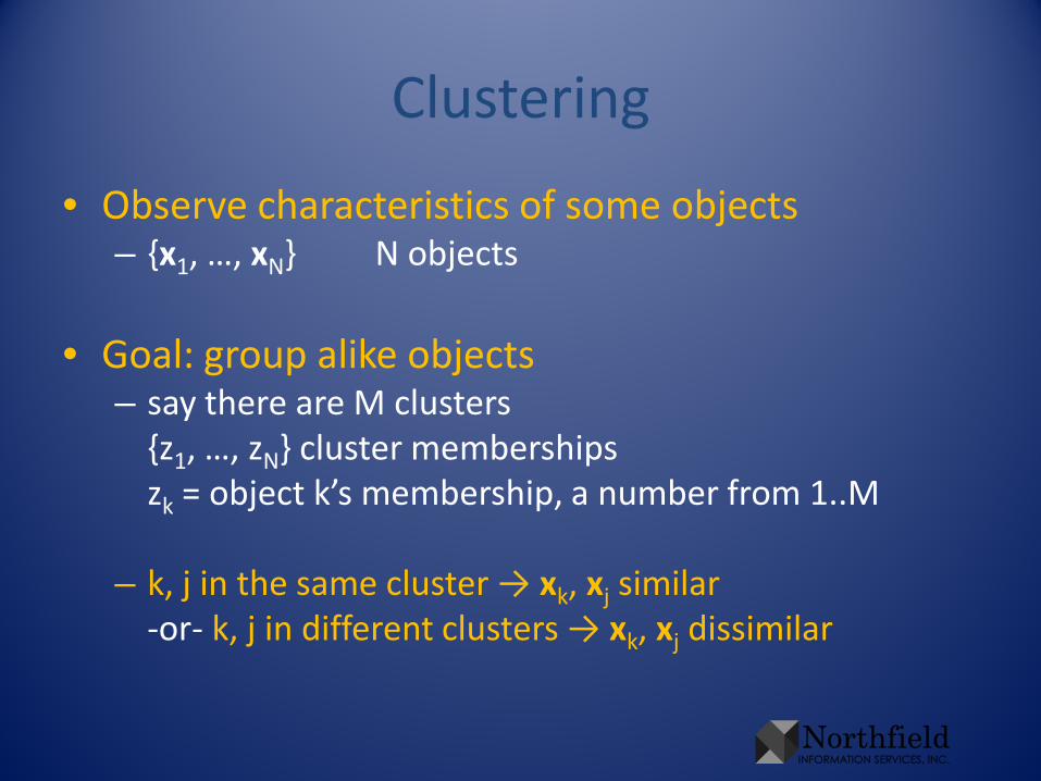
• Observe characteristics of some objects– {x1, …, xN} N objects

• Goal: group alike objects– say there are M clusters

{z1, …, zN} cluster membershipszk = object k’s membership, a number from 1..M

– k, j in the same cluster → xk, xj similar-or- k, j in different clusters → xk, xj dissimilar

Examples of Characteristics

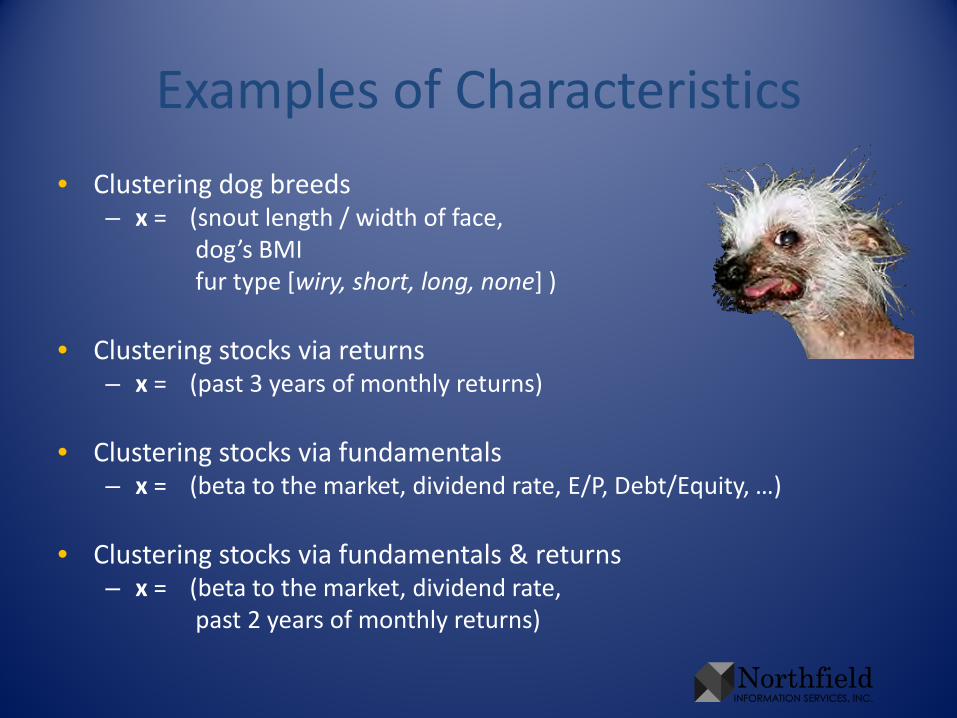
• Clustering dog breeds– x = (snout length / width of face,

dog’s BMIfur type [wiry, short, long, none] )

• Clustering stocks via returns– x = (past 3 years of monthly returns)

• Clustering stocks via fundamentals– x = (beta to the market, dividend rate, E/P, Debt/Equity, …)

• Clustering stocks via fundamentals & returns– x = (beta to the market, dividend rate,

past 2 years of monthly returns)

Machine Learning• Rather than being programmed with rules, the system inferentially learns

the patterns/rules of reality from data

• Supervised Learning– Some of the training data is labeled– e.g. There are 5 company types - AAPL & MSFT are type 1, ... , XOM is type 5.

Find the prototype for each type and label the rest of the universe– e.g. Amazon & Netflix recommendations

• Unsupervised Learning– None of the data has labels– Organize the system to maximize some criterion– e.g. Clustering maximizes similarity within each cluster– e.g. Principal Components Analysis maximizes explained variance– Vanilla clustering is the canonical example of unsupervised machine learning

Review of Forms of Hard Clustering

• ‘Hard’ means an object is assigned to only one cluster– In contrast, model-based clustering can give a probability

distribution over the clusters

• Hierarchical Clustering– Maximize distance between clusters– Flavors come from different ways of measuring distance

• Single Linkage – distance between the two nearest elements• Complete Linkage – distance between the two farthest elements• Average Linkage – mean (or median) distance between all elements

• K-Means– Minimize mean (median in K-medians) distance within clusters

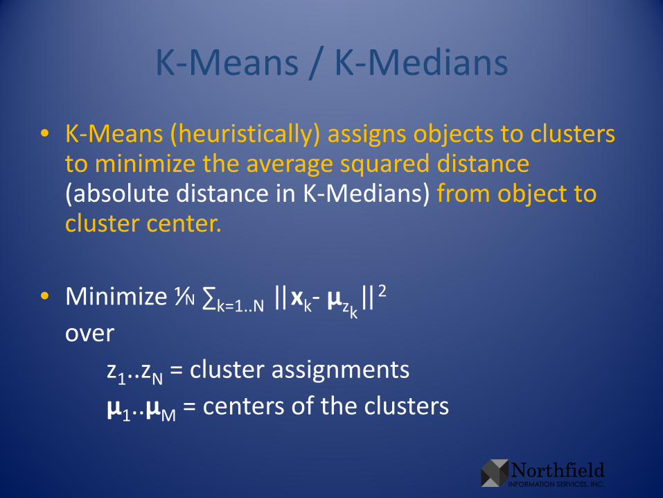
K-Means / K-Medians

• K-Means (heuristically) assigns objects to clusters to minimize the average squared distance (absolute distance in K-Medians) from object to cluster center.

• Minimize ⅟N ∑k=1..N ||xk- μzk||2

overz1..zN = cluster assignmentsμ1..μM = centers of the clusters

K-Means Algorithm

1. Randomly assign objects to clusters

2. Calculate the center (mean) of each cluster3. Check assignments for all the objects. If another center is closer to

an object, reassign the object to that cluster

4. Repeat steps 2-3 until no reassignments occur

• Extremely fast• The solution is a local max, so several starting points are used in

practice• (K-Medians) For robustness, step 2 uses median instead of mean

to get centers

Mixture of Gaussians: A Model-Based Clustering Similar to K-Means

• Observe data for N objects, {x1, …, xN}

• Each cluster generates data distributed normally around its center– when object k is from cluster m,

p(xk) ~ exp(||xk- μm||2 / σ2)

• Some clusters appear more frequently than others– given no observation information,

p(an object belongs to cluster m) = πM

• Find the setup that make the observations most likely to occur– cluster centers {μ1 .. μM}– variance σ2

– cluster frequencies {π1 .. πM}

Model-Based Clustering

• Observe characteristics of some objects– {x1, …, xN}N objects

• An object belongs to one of M clusters, but you don’t know which– {z1, …, zN} cluster memberships, numbers from 1..M

• Some clusters are more likely than others– P(zk=m) = πm (πm = frequency cluster m occurs)

• Within a cluster, objects’ characteristics are generated by the same distribution, which has free parameters– P(xk|zk=m) = f(xk, λm) (λm = parameters of cluster m)– f doesn’t have to be Gaussian

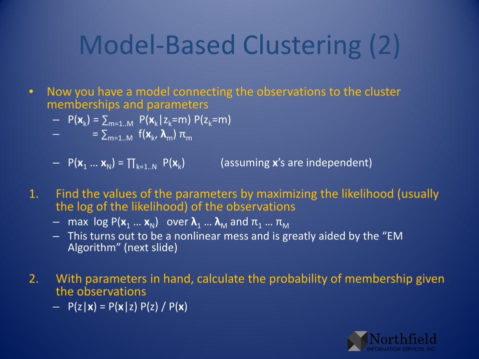
Model-Based Clustering (2)• Now you have a model connecting the observations to the cluster

memberships and parameters– P(xk) = ∑m=1..M P(xk|zk=m) P(zk=m)– = ∑m=1..M f(xk, λm) πm

– P(x1 … xN) = ∏k=1..N P(xk) (assuming x’s are independent)

1. Find the values of the parameters by maximizing the likelihood (usually the log of the likelihood) of the observations– max log P(x1 … xN) over λ1 … λM and π1 … πM– This turns out to be a nonlinear mess and is greatly aided by the “EM

Algorithm” (next slide)

2. With parameters in hand, calculate the probability of membership given the observations– P(z|x) = P(x|z) P(z) / P(x)

EM (Expectation-Maximization) Algorithm Setup

• Let θ = (λ1 … λM, π1 … πM), the parameters being maximized over

• Observe x. Don’t know z, the cluster memberships

• Want to maximize log p(x|θ), but it is too complicated

• EM can be used when– It’s possible to make an approximation of p(z|x,θ), the

conditional distribution of the hidden variables– log p(x,z|θ), the probability if all the variables were known, is

easy to manipulate

The EM Algorithm• Want to maximize log p(x|θ) = log ∫ p(x,z|θ) dz• (E Step)

– Create an approximate distribution of the missing data. Call it u(z)Ideally this is p(z|x,θ)

– Let Q(θ) = the log likelihood under θ averaged by u(z)= ∫ log p(x,z|θ) u(z) dz

• (M Step)– Maximize Q(θ) over θ– θnew = the maximizer

• Repeat E & M steps until convergence

• EM switches between 1) finding an approximate distribution of missing data given the parameters and 2) finding better parameters given the approximation

Experiments• Universe is the “S&P 468” – the S&P 500 stripped of securities missing

data• Know ICB sector assignments for these companies

– 10 sectors: Oil & Gas, Basic Materials, Industrials, Consumer Goods, Healthcare, Consumer Services, Telecommunications, Utilities, Financials, Technology

• Have information about the companies– 5 years of monthly returns– market β– fundamentals (E/P, B/P, rev/P, debt/equity, yield, trading activity, relative

strength, log mkt cap, earnings variability, growth rate, price volatility)– Each characteristic is scaled to make its cross-sectional standard deviation 1

• Using assortments of information, cluster securities into 10 groups

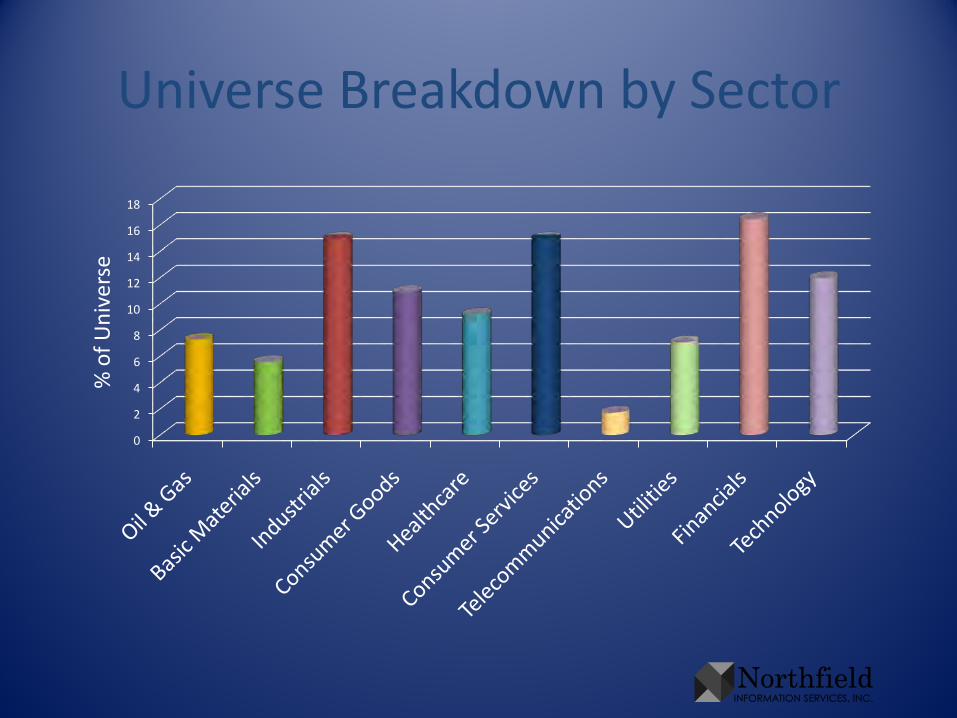
Universe Breakdown by Sector

0

2

4

6

8

10

12

14

16

18

% o

f Uni

vers

e

Cast Clusters in Termsof the Known Sectors

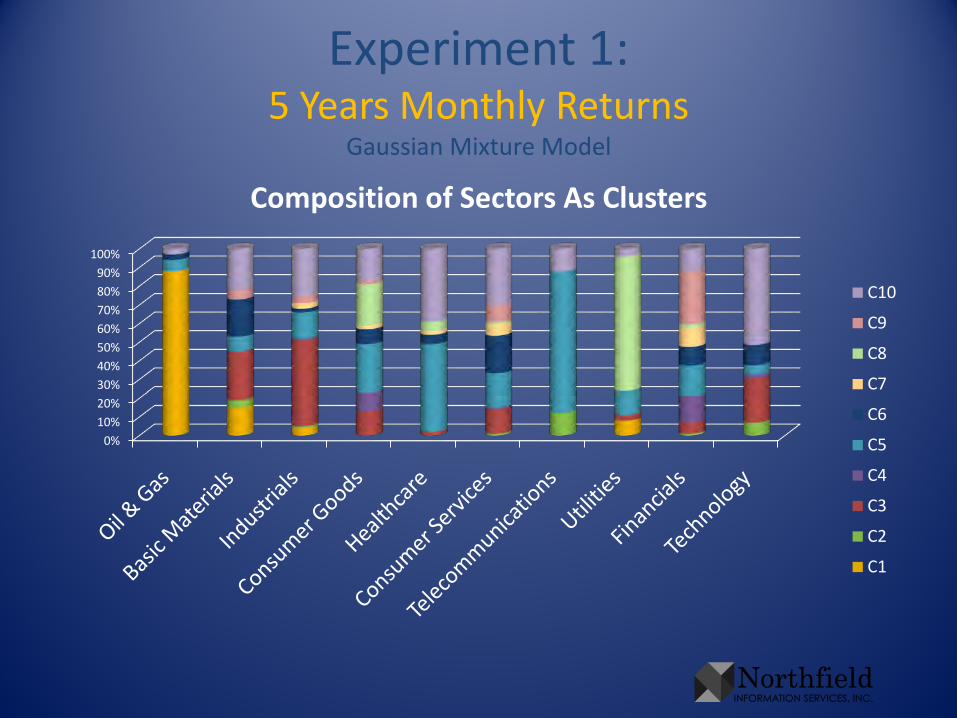
• To illustrate results in this presentation, cast the clusters in terms of the original sectors– For each sector, sum the cluster probabilities of all

companies in that sector. Rescale so the sum is 1. This gives sectors in terms of clusters

– Take that rescale in the other direction, so each cluster sums to 1. This gives the clusters in terms of sectors, without biasing toward numerous sectors

• There are many other uses for the cluster results

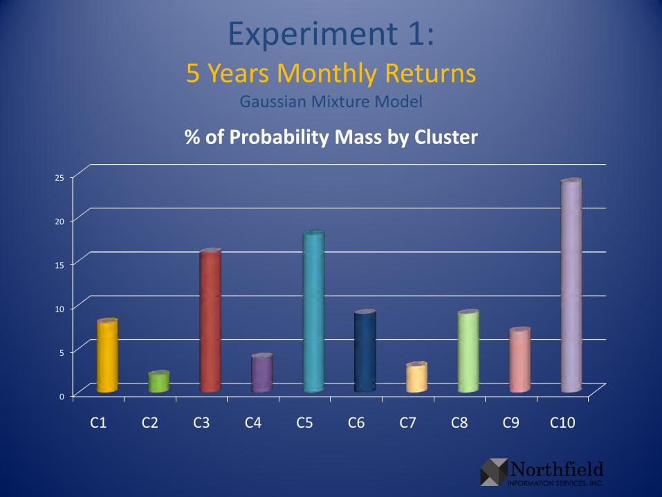
Experiment 1:5 Years Monthly Returns

Gaussian Mixture Model

0

5

10

15

20

25

C1 C2 C3 C4 C5 C6 C7 C8 C9 C10

% of Probability Mass by Cluster

Experiment 1:5 Years Monthly Returns

Gaussian Mixture Model

0%10%20%30%40%50%60%70%80%90%

100%

Composition of Sectors As Clusters

C10

C9

C8

C7

C6

C5

C4

C3

C2

C1

Experiment 1:5 Years Monthly Returns

Gaussian Mixture Model

0%

10%

20%

30%

40%

50%

60%

70%

80%

90%

100%

ABT AMZN BRK.B GE JNJ

Security Composition in Clusters

C10

C9

C8

C7

C6

C5

C4

C3

C2

C1

Experiment 1:5 Years Monthly Returns

Gaussian Mixture Model

0%

10%

20%

30%

40%

50%

60%

70%

80%

90%

100%

ABT AMZN BRK.B GE JNJ

Security Composition in Sectors

Technology

Financials

Utilities

Telecommunications

Consumer Services

Healthcare

Consumer Goods

Industrials

Basic Materials

Oil & Gas

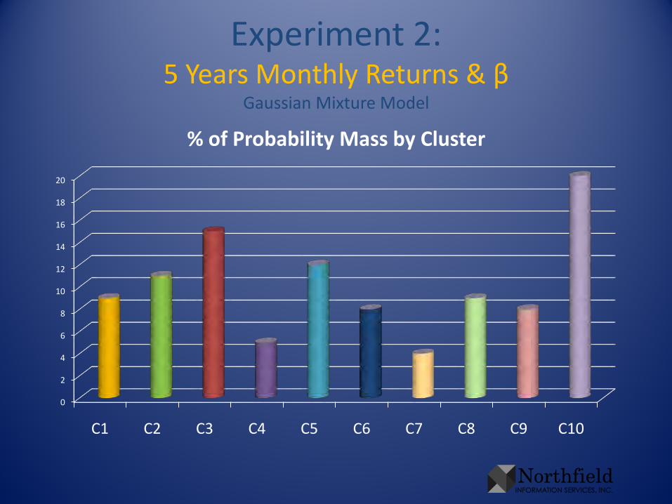
Experiment 2:5 Years Monthly Returns & β

Gaussian Mixture Model

0

2

4

6

8

10

12

14

16

18

20

C1 C2 C3 C4 C5 C6 C7 C8 C9 C10

% of Probability Mass by Cluster

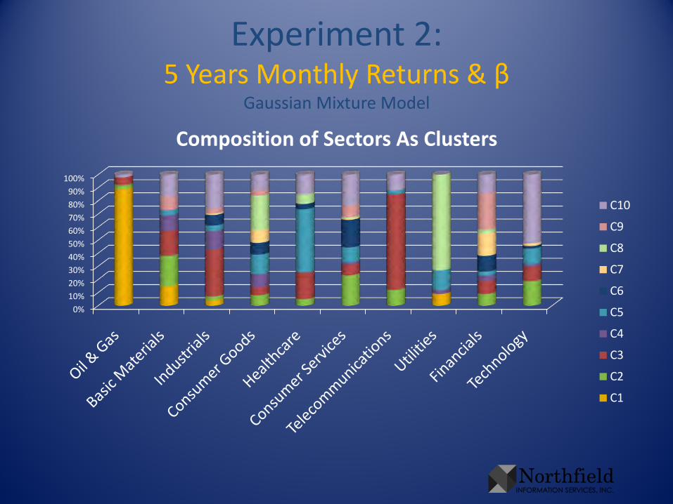
Experiment 2:5 Years Monthly Returns & β

Gaussian Mixture Model

0%10%20%30%40%50%60%70%80%90%

100%

Composition of Sectors As Clusters

C10

C9

C8

C7

C6

C5

C4

C3

C2

C1

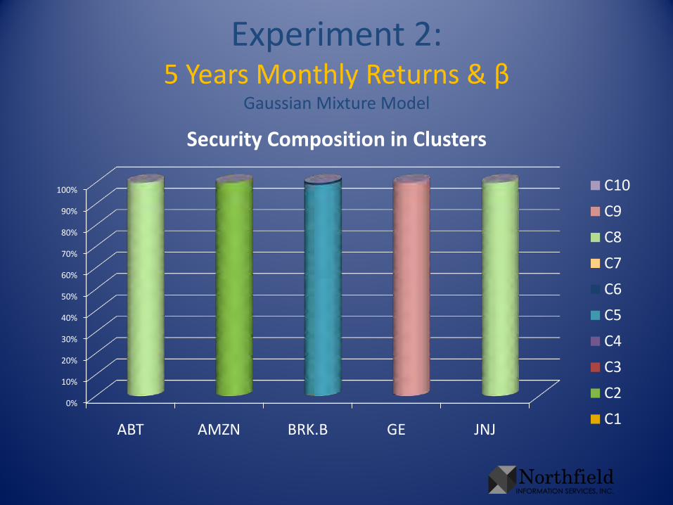
Experiment 2:5 Years Monthly Returns & β

Gaussian Mixture Model

0%

10%

20%

30%

40%

50%

60%

70%

80%

90%

100%

ABT AMZN BRK.B GE JNJ

Security Composition in Clusters

C10

C9

C8

C7

C6

C5

C4

C3

C2

C1

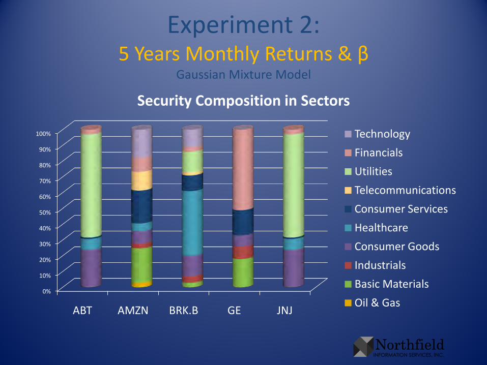
Experiment 2:5 Years Monthly Returns & β

Gaussian Mixture Model

0%

10%

20%

30%

40%

50%

60%

70%

80%

90%

100%

ABT AMZN BRK.B GE JNJ

Security Composition in Sectors

Technology

Financials

Utilities

Telecommunications

Consumer Services

Healthcare

Consumer Goods

Industrials

Basic Materials

Oil & Gas

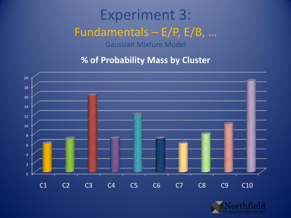
Experiment 3:Fundamentals – E/P, E/B, …

Gaussian Mixture Model

0

2

4

6

8

10

12

14

16

18

20

C1 C2 C3 C4 C5 C6 C7 C8 C9 C10

% of Probability Mass by Cluster

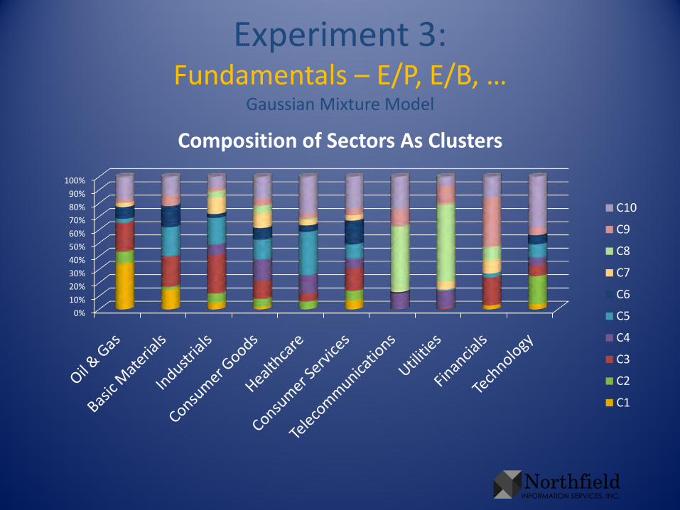
Experiment 3:Fundamentals – E/P, E/B, …

Gaussian Mixture Model

0%10%20%30%40%50%60%70%80%90%

100%

Composition of Sectors As Clusters

C10

C9

C8

C7

C6

C5

C4

C3

C2

C1

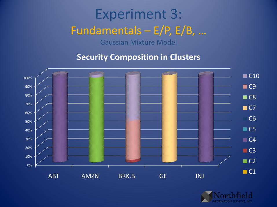
Experiment 3:Fundamentals – E/P, E/B, …

Gaussian Mixture Model

0%

10%

20%

30%

40%

50%

60%

70%

80%

90%

100%

ABT AMZN BRK.B GE JNJ

Security Composition in Clusters

C10

C9

C8

C7

C6

C5

C4

C3

C2

C1

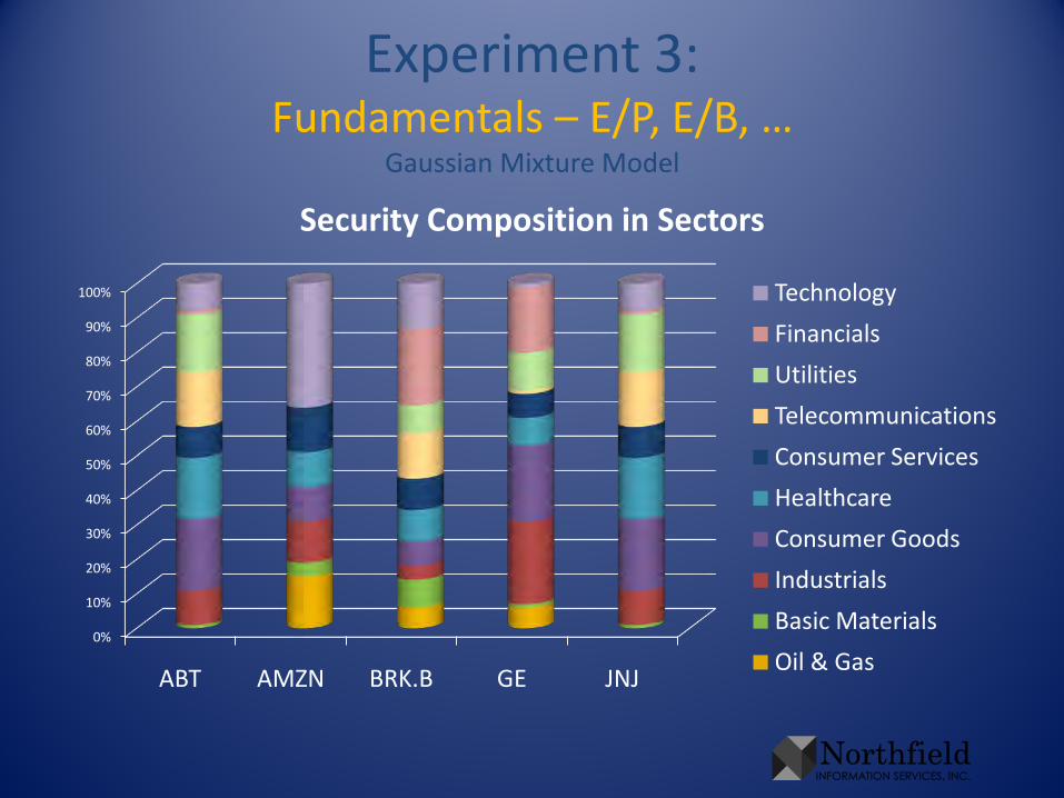
Experiment 3:Fundamentals – E/P, E/B, …

Gaussian Mixture Model

0%

10%

20%

30%

40%

50%

60%

70%

80%

90%

100%

ABT AMZN BRK.B GE JNJ

Security Composition in Sectors

Technology

Financials

Utilities

Telecommunications

Consumer Services

Healthcare

Consumer Goods

Industrials

Basic Materials

Oil & Gas

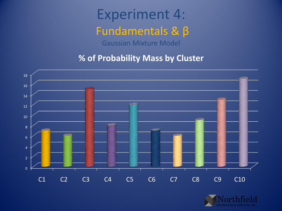
Experiment 4:Fundamentals & β

Gaussian Mixture Model

0

2

4

6

8

10

12

14

16

18

C1 C2 C3 C4 C5 C6 C7 C8 C9 C10

% of Probability Mass by Cluster

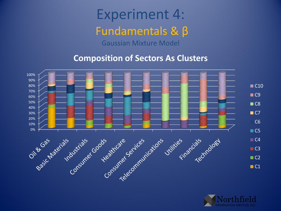
Experiment 4:Fundamentals & β

Gaussian Mixture Model

0%10%20%30%40%50%60%70%80%90%

100%

Composition of Sectors As Clusters

C10

C9

C8

C7

C6

C5

C4

C3

C2

C1

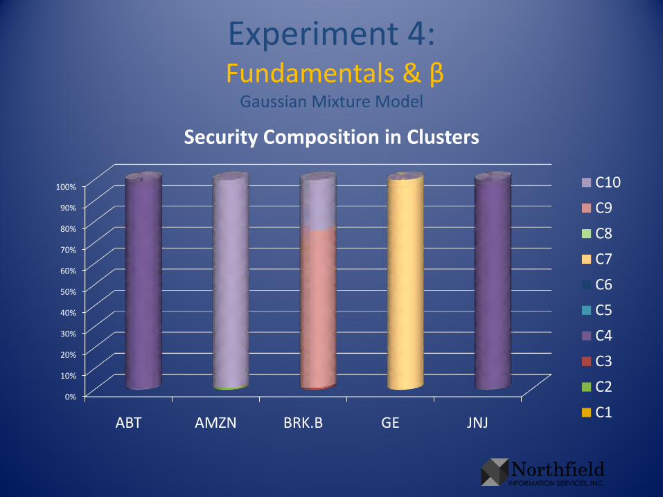
Experiment 4:Fundamentals & β

Gaussian Mixture Model

0%

10%

20%

30%

40%

50%

60%

70%

80%

90%

100%

ABT AMZN BRK.B GE JNJ

Security Composition in Clusters

C10

C9

C8

C7

C6

C5

C4

C3

C2

C1

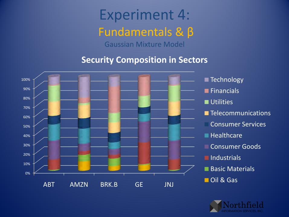
Experiment 4:Fundamentals & β

Gaussian Mixture Model

0%

10%

20%

30%

40%

50%

60%

70%

80%

90%

100%

ABT AMZN BRK.B GE JNJ

Security Composition in Sectors

Technology

Financials

Utilities

Telecommunications

Consumer Services

Healthcare

Consumer Goods

Industrials

Basic Materials

Oil & Gas

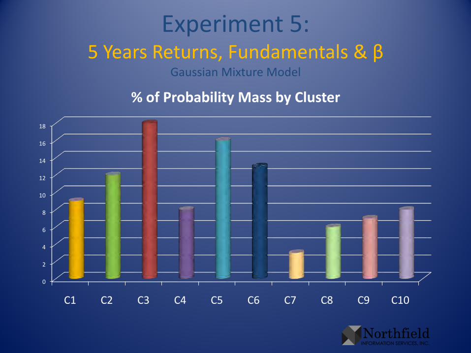
Experiment 5:5 Years Returns, Fundamentals & β

Gaussian Mixture Model

0

2

4

6

8

10

12

14

16

18

C1 C2 C3 C4 C5 C6 C7 C8 C9 C10

% of Probability Mass by Cluster

Experiment 5:5 Years Returns, Fundamentals & β

Gaussian Mixture Model

0%10%20%30%40%50%60%70%80%90%

100%

Composition of Sectors As Clusters

C10

C9

C8

C7

C6

C5

C4

C3

C2

C1

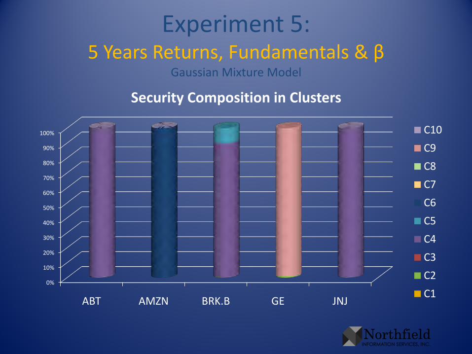
Experiment 5:5 Years Returns, Fundamentals & β

Gaussian Mixture Model

0%

10%

20%

30%

40%

50%

60%

70%

80%

90%

100%

ABT AMZN BRK.B GE JNJ

Security Composition in Clusters

C10

C9

C8

C7

C6

C5

C4

C3

C2

C1

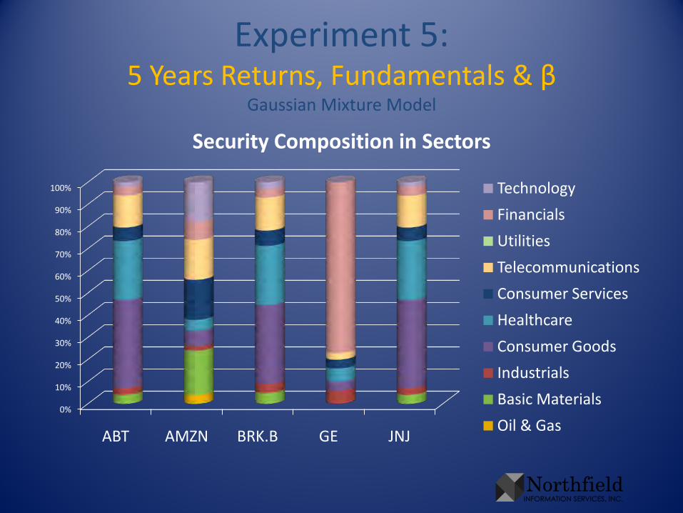
Experiment 5:5 Years Returns, Fundamentals & β

Gaussian Mixture Model

0%

10%

20%

30%

40%

50%

60%

70%

80%

90%

100%

ABT AMZN BRK.B GE JNJ

Security Composition in Sectors

Technology

Financials

Utilities

Telecommunications

Consumer Services

Healthcare

Consumer Goods

Industrials

Basic Materials

Oil & Gas

Closing Remarks

• It works with different distributions– Here, deviations from cluster centers were Gaussian– Can easily do the same assuming deviations

~ e-λ|x|, the distribution associated with median. (Gaussian is mean)

• Clustering helps identify what a security is, i.e. what alpha model to use for it

• Switching from applying filters to thinking about underlying mathematical models– gives you your own custom tool set– makes understanding what something does infinitely easier