AN INTEGRATED STOCK MARKET FORECASTING MODEL USING

AN INTEGRATED STOCK MARKET FORECASTING MODEL USING NEURAL

NETWORKS

A thesis presented to

the faculty of

the Fritz J. and Dolores H. Russ

College of Engineering and Technology of Ohio University

In partial fulfillment

of the requirements for the degree

Master of Science

Sriram Lakshminarayanan

August 2005

This thesis entitled

AN INTEGRATED STOCK MARKET FORECASTING MODEL USING NEURAL

NETWORKS

By


has been approved for

the Department of Industrial and Manufacturing Systems Engineering

and the Russ College of Engineering and Technology by

Gary R. Weckman

Associate Professor of Industrial & Manufacturing Systems Engineering

Dennis Irwin Dean, Fritz J. and Dolores H. Russ

College of Engineering and Technology

LAKSHMINARAYANAN SRIRAM. M.S. August 2005. Industrial and Manufacturing

Systems Engineering

An Integrated Stock Market Forecasting Model Using Neural Networks (126pp.)

Director of Thesis: Gary Weckman

This thesis focuses on the development of a stock market forecasting model based

on an Artificial Neural Network architecture. This study constructs a hybrid model

utilizing various technical indicators, Elliott’s wave theory, sensitivity analysis and fuzzy

logic. Initially, a baseline network is constructed based on available literature. The

baseline model is then improved by applying several useful information domains to the

different models. Optimizations of the Neural Network models are performed by

augmenting the network with useful information at every stage.

Approved:

Gary Weckman

Associate Professor of Industrial and Manufacturing Systems Engineering

5

TABLE OF CONTENTS

ABSTRACT........................................................................................................................ 4

LIST OF FIGURES ............................................................................................................ 8

LIST OF TABLES............................................................................................................ 10

CHAPTER 1. INTRODUCTION ................................................................................ 11

1.1 Description of Forecasting ........................................................................................... 11

1.2 Forecasting Problems ................................................................................................... 12

1.3 Previous Research ........................................................................................................ 13

1.4 Current Research .......................................................................................................... 14

1.5 Thesis Structure ............................................................................................................ 15

CHAPTER 2. BACKGROUND .................................................................................. 17

2.1 Artificial Neural Networks ........................................................................................... 17

2.1.1 Introduction ...........................................................................................................................17

2.1.2 Applications of Neural Networks ..........................................................................................18

2.1.3 Common Classification of Neural Networks.........................................................................19

2.1.4 Neural Network Architectures and Training .........................................................................20

2.1.5 Neural-Network Training ......................................................................................................27

2.2 Elliott’s Wave Theory .................................................................................................. 30

2.2.1 History...................................................................................................................................30

6

2.2.2 Principles of Elliott Wave Theory .........................................................................................30

2.2.3 Fibonacci Series and Elliott’s Wave Theory .........................................................................34

2.3 Stock Market Indicators ............................................................................................... 36

2.3.1 Introduction ...........................................................................................................................36

2.3.2 Classification of Indicators....................................................................................................37

2.3.3 Basic Indicators .....................................................................................................................38

2.4 Fuzzy Logic .................................................................................................................. 42

2.4.1 Introduction to Fuzzy Logic ..................................................................................................42

2.4.2 Fuzzy Set Theory...................................................................................................................43

CHAPTER 3. METHODOLOGY ............................................................................... 46

3.1 Stock Market Data........................................................................................................ 46

3.2 Analysis of Preliminary Indicators ............................................................................... 49

3.3 Indicator Selection Using Self Organizing Map........................................................... 50

3.4 Elliott Wave Implementation........................................................................................ 55

3.5 Summary....................................................................................................................... 57

CHAPTER 4. RESULTS AND DISCUSSION........................................................... 58

4.1 Performance of the Benchmark Network ..................................................................... 58

4.2 Indicator Analysis using Self Organizing Maps........................................................... 63

7

4.3 Elliott Wave Indicators Implementation....................................................................... 69

CHAPTER 5. CONCLUSIONS AND FUTURE RESEARCH .................................. 75

5.1 Conclusions .................................................................................................................. 75

5.2 Future Research ............................................................................................................ 77

REFERENCES ................................................................................................................. 79

APPENDIX A................................................................................................................... 82

APPENDIX B ................................................................................................................... 97

APPENDIX C ................................................................................................................. 112

8

LIST OF FIGURES

Figure 2-1 Schematic Diagram of a Neural Network ....................................................... 18

Figure 2-2 Functional Diagram of Perceptron .................................................................. 21

Figure 2-3 Generalized Feed Forward Nework (Adapted from NeuroSolutions) ............ 23

Figure 2-4 Sigmoid Function ............................................................................................ 24

Figure 2-5 Gaussian Function........................................................................................... 25

Figure 2-6 2-D Kohonen Self Organizing Map (Adapted from [18]) .............................. 26

Figure 2-7 Cross Validation during Training.................................................................... 29

Figure 2-8 Elliott's Five Wave Pattern.............................................................................. 31

Figure 2-9 A Typical Elliott Wave Cycle. (Adapted from [13]) ...................................... 33

Figure 2-10 Fibonacci Ratios in Elliott Wave .................................................................. 35

Figure 2-11 Fibonacci Ratio Possibilities in Elliot Wave................................................. 35

Figure 2-12 Fuzzy Sets Example ...................................................................................... 44

Figure 2-13 Fuzzy System Schematic Diagram (Adapted from [20] )............................. 45

Figure 3-1 Generalized Feed Forward Network as represented by NeuroSolutions ........ 49

Figure 3-2 NeuroSolutions Representation of a Self Organizing Map............................. 52

Figure 3-3 Final Generalized Feed Forward Network implementation............................ 54

Figure 3-4 Self Organizing Map Methodology ................................................................ 54

Figure 3-5 Probability of Data being Turning Point ......................................................... 56

Figure 3-6 Forecasting Decisions ..................................................................................... 56

9

Figure 3-7 Methodology ................................................................................................... 57

Figure 4-1 MLP Network Performance of AGP............................................................... 61

Figure 4-2 GFF Network Performance of AGP................................................................ 61

Figure 4-3 Distribution of Actual vs. Predicted Close of AGP ........................................ 62

Figure 4-4 GFF with SOM Indicators Output .................................................................. 68

Figure 4-5 Final Network Output ..................................................................................... 71

Figure 4-6 Predicted vs. Actual Closing Price Comparison ............................................. 72

Figure 4-7 Relative Sensitivity of Indicators .................................................................... 74

10

LIST OF TABLES

Table 3-1 Stocks Analyzed ............................................................................................... 48

Table 3-2 Input Indicators to a Self Organizing Map Network ........................................ 51

Table 3-3 SOM Indicators Coding Methodology ............................................................. 53

Table 4-1 Performance Measures ..................................................................................... 58

Table 4-2 Initial Performance Statistics for AGP............................................................. 59

Table 4-3 Performance of Benchmark Model .................................................................. 60

Table 4-4 SOM Indicators Coding Methodology ............................................................. 64

Table 4-5 SOM Indicators ................................................................................................ 65

Table 4-6 GFF Performance after SOM of AGP............................................................. 66

Table 4-7 Performance of SOM Model ............................................................................ 67

Table 4-8 Price Movement Prediction Results ................................................................. 69

Table 4-9 Final Network Performance ............................................................................. 70

Table 4-10 Final Network Performance ........................................................................... 70

Table 4-11 Final Change Prediction Results .................................................................... 72

Table 4-12 Indicators used in Sensitivity Analysis........................................................... 73

11

CHAPTER 1. INTRODUCTION

1.1 Description of Forecasting

Forecasting is the process of making projections about future performance based on

existing historic data. An accurate forecast aids in decision-making and planning for the

future. Forecasts empower people to modify current variables in the present to predict the

future to result in a favorable scenario.

The selection and implementation of a proper forecasting methodology has

always been an important planning and control issue for most firms and agencies. The

organizational and financial stability of an organization depends on the accuracy of the

forecast since such information will most likely be used to make key decisions in the

areas of human resources, purchasing, marketing, advertising and capital financing.

When a variable is to be predicted, the difficulty of forecasting depends on

various factors. Most importantly, the historic pattern of the variable and the underlying

input factors that affect a variable may increase the complexity of the forecasting task. A

volatile historic pattern may suggest that the factor to be forecast has a number of

underlying factors, the effects of each dynamically changing over time. Some of these

contributing factors may not be identifiable and hence require an amount of expert

knowledge gained over time to be built into the forecasting model.

12

Forecasting a financial scenario such as the stock market would be a very

important step when assessing the prudence of an investment. This step is very difficult

due to complexity and presence of a multitude of factors that may affect the value of a

certain financial instrument [4].

1.2 Forecasting Problems

The following are the major challenges that are identified in the field of

forecasting

1. In certain cases, it may be difficult to ascertain a future scenario during

forecasting. Regardless of the techniques that may be used, it is always assumed

that there will be a variable measure of uncertainty.

2. Forecasting variables for which there are no existing paradigms or historical data

is often prone to errors, primarily due to the lack of ability to understand

underlying factors which could affect the forecast [1][40].

3. Selection and implementation of a proper forecasting methodology is very

important due to the fact that different forecasting problems must to be addressed

using different tailor made models to suit each [8].

13

1.3 Previous Research

Stock market forecasting involves the analysis of several hundred indicators to

augment the decision making process. Stock market indicators are mostly proven

statistical functions, some of which are very similar in nature [1]. Analysts are required to

identify indicators that are useful to them by meticulous screening methods that may be

time consuming and may have some undesired financial repercussions. Stock market

trading has been considered a risky and volatile business and traders have generally

resorted to two broad types of analysis [6]; use of traditional, proven indicators and the

interpretation of patterns and charts. Using the former technique provides mediocre

accuracy with a lower risk limit, while the latter provides high accuracy with a higher risk

limit. The current research on stock market forecasting involves artificial intelligence

techniques and real time computing to utilize the advantages of the above mentioned

traditional techniques and provide an accurate forecast with a high confidence limit. One

study required high computing power and a substantial amount of time for increasing the

accuracy of the model [9].

Artificial Neural Networks have been used by several researchers for developing

applications to help make more informed financial decisions. Simple Neural Network

models do a reasonably good job of predicting stock market price motion, with buy/sell

prediction accuracies considerably higher than traditional models. This performance is

being improved by adding more complexity to the network architecture and using more

14

historical data. Different types of network architectures such as Multi Layer Perceptrons,

Generalized Feed Forward networks and Radial Basis Functions are becoming

increasingly popular and are being tested for higher accuracy. Many researchers are also

investigating the possibility of adding additional indicators that may help the Neural

Network improve training and performance while testing on production data. Neural

Networks show potential for minimizing forecasting errors due to the improvements

made in training algorithms and increased availability of indicators.

1.4 Current Research

The research by Bogullu et al [6] involves training the Feed Forward Neural

Networks to generate Buy – Sell trading signals. The predictability and the profitability

results given by the trained Neural Networks are compared against rule-based models of

the technical indicators [14]. Technical indicators are useful tools in predicting the

direction of stock prices. However they suffer from the linguistic uncertainty that is

inherent in any decisions resulting from heuristic based trading rules [15]. Several

interesting questions arise in connection with the current research:

1. Can higher accuracy be generated by increasing network input factors without

compromising the processing complexity and time?

2. Is additional data required if the number of input factors are increased for

efficient learning?

15

3. Can the newly formulated network outperform the networks used for Baseline

comparisons?

In light of these questions, this research has extended the work of Weckman et al [40].

This work initially replicates the models of Weckman et al [1] [40] by developing

a network using the known baseline indicators. Next, additional indicators are used to

improve the network’s performance. The network indicators are then pruned by using a

Self Organizing Map. The performance altering Elliott’s wave indicator used fuzzy logic

techniques to classify the probability of a trend change. To simulate real time trading, the

final performance measure was buy/sell decisions. This ensemble of techniques was

applied to stocks from five different sectors and three different growth/value sizes of the

particular industry. This thesis presents an approach for incorporating enhanced

techniques into the forecasting process.

1.5 Thesis Structure

The thesis has been organized into five chapters and is explained as follows. Chapter

1 introduces the forecasting problem and summarizes the previous and current work

completed in the intended research. Chapter 2 provides background and literature survey

of related work in stock market forecasting problems. It also covers the concepts of

Neural Networks and its application to forecasting, as well as giving coverage of the

areas of Elliott’s wave theory and Indicator Analysis. Chapter 3 presents the

16

methodology adopted for generating forecasting models using Neural Networks and

model optimization techniques. Chapter 4 discusses the results of the forecasting models

and analyzes the applicability of the technique to different types of stocks. Chapter 5

provides conclusions and suggestions for future implementation.

17

CHAPTER 2. BACKGROUND

This chapter discusses the background and related work in the area of forecasting

using Artificial Neural Networks.

2.1 Artificial Neural Networks

2.1.1 Introduction

An Artificial Neural Network is defined as an information-processing paradigm

inspired by the methods by which the mammalian brain processes information [7] [24]

presented to it. They are an assortment of mathematical models that imitate some of the

observed phenomena in a biological nervous system, most importantly adaptive

biological learning. One unique and important property of the Artificial Neural Network

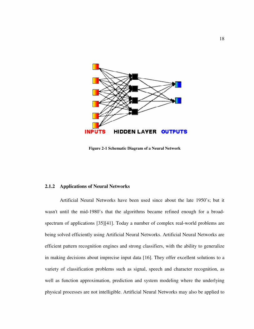
model is the exceptional structure of the information processing system [34]. It is made

of a number of highly interconnected processing elements that are very similar to neurons

and are joined by weighted connections that are very similar to synapses (Figure 2-1).

18

Figure 2-1 Schematic Diagram of a Neural Network

2.1.2 Applications of Neural Networks

Artificial Neural Networks have been used since about the late 1950’s; but it

wasn't until the mid-1980’s that the algorithms became refined enough for a broad-

spectrum of applications [35][41]. Today a number of complex real-world problems are

being solved efficiently using Artificial Neural Networks. Artificial Neural Networks are

efficient pattern recognition engines and strong classifiers, with the ability to generalize

in making decisions about imprecise input data [16]. They offer excellent solutions to a

variety of classification problems such as signal, speech and character recognition, as

well as function approximation, prediction and system modeling where the underlying

physical processes are not intelligible. Artificial Neural Networks may also be applied to

19

solve control system problems, where the input variables are calculated and used to drive

an output variable and the network learns the control function. A key advantage of

Artificial Neural Networks lies in their flexibility against aberrations in the input

variables and their latent potential of learning. They have been frequently identified as

proficient at solving problems that are multifarious for conservative technologies (e.g.,

problems that do not have an algorithmic/heuristic solution process) and are often well

suited to problems that are required to mimic biological intelligence[39].

2.1.3 Common Classification of Neural Networks

There are various architectures of Artificial Neural Networks that are commonly

used. A very popular network architecture is the Multilayer Perceptron [28][26] which is

generally trained with the back propagation of error, learning vector quantization, radial

basis function, Hopfield, and Kohonen algorithms [18]. Some Artificial Neural Networks

are classified as Feed Forward while others maybe recurrent (i.e., implement feedback)

depending on the method of training employed and data processing through the network.

Another popular method of classifying Artificial Neural Networks is by the training

algorithms used, as some Artificial Neural Networks employ supervised training while

others utilize unsupervised or self-organizing[20][21]. Supervised training methods are

used when the network learns from a training set of data that has an output associated

with each set of input. Unsupervised algorithms [12] effectively perform clustering of the

data into similar groups based on the calculated attributes serving as inputs to the

algorithms.

20

2.1.4 Neural Network Architectures and Training

Training is the procedure by which the Neural Network learns and understands

the relationship between the input and the output variables. Learning in biological

systems may be considered as modifications made to the weights (synaptic connections)

that exist between the neurons [3]. Learning or training in an Artificial Neural Network is

brought about by introduction of the network to a validated set of input/output data where

the training algorithm iteratively adjusts the synaptic connection weights. These

connection weights store the information learned by the network and are necessary to

solve specific problems during the testing phase of the network validation process.

Neural Networks are characterized by the following properties:

• The pattern of connections between the various network layers (Network type)

• Number of neurons in each layer (complexity)

• Learning algorithm

• Neuron activation functions

Generally speaking, a Neural Network is a set of connected input and output units

where each connection has a weight associated with it. The learning phase involves the

network’s ability to adjust the weights so as to be able to correctly forecast or classify the

output target of a given set of input data. Given the numerous types of Neural Network

architectures that have been developed in the literature, the important types of Neural

Networks often used for forecasting and classification problems are discussed.

21

2.1.4.1 Multilayer Perceptrons:

Multilayer Perceptrons are layered Feed Forward networks classically trained

with static back propagation algorithms. These networks are extensively used in countless

applications requiring static pattern classification. Their key property is that they are easy

to use, and that they can approximate any input/output map. The key disadvantages are

that they train relatively slowly, and require comparatively a large amount of training

data sets [2].

Figure 2-2 Functional Diagram of Perceptron

y

xn

x2

x1

w2

w1

wn wb= 1

b

� (.)

22

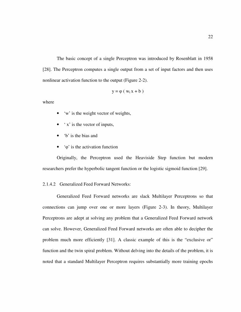
The basic concept of a single Perceptron was introduced by Rosenblatt in 1958

[28]. The Perceptron computes a single output from a set of input factors and then uses

nonlinear activation function to the output (Figure 2-2).

y = � ( wt x + b )

where

• ‘w’ is the weight vector of weights,

• ‘ x’ is the vector of inputs,

• ‘b’ is the bias and

• ‘�’ is the activation function

Originally, the Perceptron used the Heaviside Step function but modern

researchers prefer the hyperbolic tangent function or the logistic sigmoid function [29].

2.1.4.2 Generalized Feed Forward Networks:

Generalized Feed Forward networks are slack Multilayer Perceptrons so that

connections can jump over one or more layers (Figure 2-3). In theory, Multilayer

Perceptrons are adept at solving any problem that a Generalized Feed Forward network

can solve. However, Generalized Feed Forward networks are often able to decipher the

problem much more efficiently [31]. A classic example of this is the “exclusive or”

function and the twin spiral problem. Without delving into the details of the problem, it is

noted that a standard Multilayer Perceptron requires substantially more training epochs

23

than the Generalized Feed Forward network containing a comparative amount of

processing elements.

Figure 2-3 Generalized Feed Forward Nework (Adapted from NeuroSolutions)

2.1.4.3 Radial Basis Function:

Radial basis function networks are a type of nonlinear hybrid networks generally

containing a single hidden layer of Perceptrons. The hidden layer generally uses Gaussian

transfer functions (Figure 2-5), rather than the standard Sigmoidal functions (Figure 2-4)

used by Multilayer Perceptrons.

24

Figure 2-4 Sigmoid Function

The properties of the Gaussian transfer functions (Figure 2-5), namely the center

and width are determined by unsupervised learning rules. The output layer typically

involves supervised learning. These networks have a very high learning rate when

compared to Multilayer Perceptrons.

25

Figure 2-5 Gaussian Function

When a Generalized regression or probabilistic net is chosen, all the weights of

the network can be computed analytically. This type of Radial basis function networks

are employed only when the number of exemplars is small (<100) or dispersed thereby

making clustering ill defined.

2.1.4.4 Self Organizing Maps

One of the most important issues in pattern recognition is feature extraction. Since

this is such a crucial step, different techniques may provide a better fit to our problem.

The ideas of Self Organizing Maps are rooted in competitive learning networks [17].

These nets are one layer nets with linear processing elements but use a competitive

learning rule. In such nets there is one and only one winning element for every input

v

f(v)

26

pattern (i.e. the element whose weights are closest to the input pattern). Kohonen [19]

proposed a slight modification of this principle with tremendous implications. Instead of

updating only the winning element, in Self Organizing Maps the neighboring element

weights are also updated with a smaller step size. This implies that in the learning process

(topological) neighborhood relationships are created in which the spatial locations

correspond to features of the input data. The data points that are similar in input space are

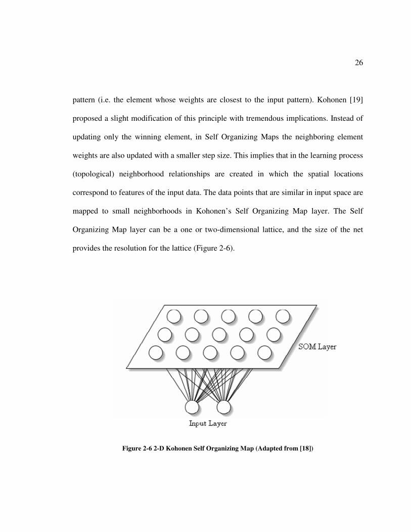
mapped to small neighborhoods in Kohonen’s Self Organizing Map layer. The Self

Organizing Map layer can be a one or two-dimensional lattice, and the size of the net

provides the resolution for the lattice (Figure 2-6).

Figure 2-6 2-D Kohonen Self Organizing Map (Adapted from [18])

27

2.1.5 Neural-Network Training

The training phase in Neural Networks determines the following important

parameters for a superior performance of the network

• Network parameters such as weights and biases that allow a network to map a

given set of input patterns to desired outputs

• Method of determination of these parameters

The back propagation algorithm is a very commonly used training algorithm. The

term back-propagation refers to the direction of propagation of error. The single most

important goal of the training regimen is to adjust the weights and biases of the network

in order to minimize the error in the output function also called the cost function. The

fundamental idea is that the cost function has a particular surface over the weight space

and therefore an iterative process such as the gradient descent method can be used for its

minimization. The gradient descent method is based on the fact that the gradient of a

function always points towards the direction of maximum increase of the function and

therefore a negative gradient will provoke a “downhill” movement eventually reaching

the minimum of the cost function. The single most important insight while using this

method is that the function may mistake a local minimum for a global minimum.

Therefore caution needs to be taken during the development of the model to avoid this

incident.

The cost function, E needs to be minimized and its derivative with respect to the

weight is calculated and denoted by ∂E/∂w. Having obtained the derivative, the problem

28

of adjusting weights is an optimization problem. Back-propagation uses a form of

gradient descent [38] to update weights according to the formula:

ijij w

Ew

∂∂−=∆ η

Where,

• wij denotes the weight of the synapse from node i to node j.

• η > 0 is the learning rate and

• ∂E/∂wij, is the partial derivative of the error, E with respect to weight wij.

The network is generally initialized with random weights and the training algorithm

modifies the weights as discussed above. Many alternative optimization techniques have

been utilized. Variations of the basic method include methods such as the conjugate-

gradient method, momentum learning, etc. Convergence to local minima can be avoided

by using stochastic search algorithms like simulated annealing and genetic algorithms.

Since these methods are global optimization procedures, they require longer times to run

and are therefore costly to implement.

A collection of input and output factors used to train the learning system is called

the training set. The testing set contains exemplars (data) that are not used for the training

purpose. The testing set is generally used to evaluate the generalization capabilities of the

network. A very important phenomenon while using the back-propagation algorithm is

that the performance always improves with the number of training cycles or epochs.

29

However, the error on the testing set initially decreases with the number of cycles, and

then increases (Figure 2-7).

Figure 2-7 Cross Validation during Training

This phenomenon is called overtraining and is indicative of poor generalization

capabilities. One solution to this problem is to split the training set into two sets – the

initial training set and the validation set. After every fixed number of iterations, the error

on the validation set is calculated. Training is terminated when this error starts to

increase. This method is called early stopping or stopping with cross-validation.

Training Data

Testing Data

Cut-Off point

Epochs

Fore

cast

ing

Err

or

30

2.2 Elliott’s Wave Theory

2.2.1 History

Ralph Nelson Elliott was a businessman who discovered a sequence of waves,

which reoccurred in stock market trading over a particular period of time. Elliott refined

his studies and published the results initially in a monograph titled “The Wave Principle”

in 1938. He published more on this principle in a sequence of articles in the Financial

World magazine during 1939. He added to the Wave Principle by publishing another

famous monograph in early 1946 titled Nature’s Law. His work also contained a

collection of various interpretive letters between 1938 and 1947 [13].

The wave theory according to R.N.Elliott was not only present in organized

financial markets, but also in all human actions and advancements. Waves of different

degrees arise regardless of the presence or absence of recording machinery. When the

machinery is present, the patterns of waves are perfected and become visible to the

experienced eye [27].

2.2.2 Principles of Elliott Wave Theory

The Elliott’s wave theory is based on the fundamental premise that the stock

market has a hidden order associated with it according to which the market moves [11].

The Elliott Wave Principle consists of empirically derived concepts developed after an

extensive study of stock market movements. The form and structure of waves that was

31

uncovered is simple to understand and elegant in its basic expression. It was discovered

that all stock market movements typically occur in eight waves or sequences. Each wave

in this sequence is a financial move that inhabits a programmed position consisting of

direction and duration with a relation to the magnitude of the other 7 waves in the

sequence. A 5-wave upward or bullish trend sequence rarely ends with an irregular set of

waves at the top part of the movement. This results in an A-wave correction that is

common, but the upward B-wave has a magnitude greater than the previous fifth wave.

Due to this corrective trend in the bull market, the next C-wave correction is straight

down, more severe in magnitude and lasts longer than a typical ABC correction.

Figure 2-8 Elliott's Five Wave Pattern

32

The Figure 2-8 explains the bull market phase of five waves consisting of three

waves up (Waves 1, 3, and 5), with two corrective waves down (waves 2 and 4). This is

followed by three waves down (ABC Waves) in the bear phase of the cycle, completing

the eight-wave sequence. It was further noted that these eight wave sequences appeared

one after another and became part of a larger wave sequence. The naming convention

started by analysts resulted in naming the smallest wave observed as a subminuette wave,

and the waves were named in order of rising magnitude as follows:

• Subminuette

• Minuette

• Minute

• Minor

• Intermediate

• Primary

• Cycle

• Super cycle

• Grand super cycle

The most important principle in understanding the Elliott Wave Principle is that

wave structures of the largest degree are composed of smaller sub waves, which are in

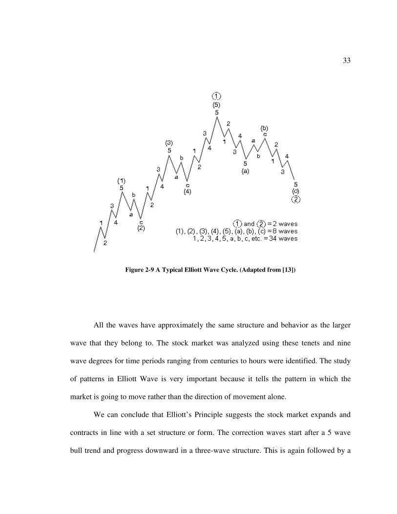
turn composed of even smaller sub waves, and so on (Figure 2-9).

33

Figure 2-9 A Typical Elliott Wave Cycle. (Adapted from [13])

All the waves have approximately the same structure and behavior as the larger

wave that they belong to. The stock market was analyzed using these tenets and nine

wave degrees for time periods ranging from centuries to hours were identified. The study

of patterns in Elliott Wave is very important because it tells the pattern in which the

market is going to move rather than the direction of movement alone.

We can conclude that Elliott’s Principle suggests the stock market expands and

contracts in line with a set structure or form. The correction waves start after a 5 wave

bull trend and progress downward in a three-wave structure. This is again followed by a

34

five-wave bull (upward) momentum structure. An important conclusion of this

fundamental tenet indicates that prices do not return to the low point of the previous 8

wave sequence, prices only approach the previous low.

2.2.3 Fibonacci Series and Elliott’s Wave Theory

The Fibonacci series is the mathematical backbone of the Elliott’s Wave Theory

[10]. The properties of this sequence appear throughout nature and also in the arts and

sciences. The ratio of 1.618, also called as the "Golden Mean", is very common in nature.

It is obtained by dividing the Fibonacci number by its preceding number as the sequence

extends into infinity. The ratio of 0.618, which is the inverse of 1.618, is also used in

analyzing the wave patterns.

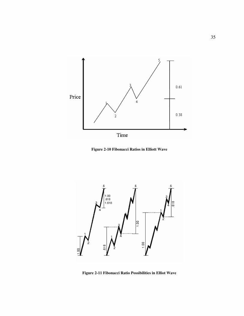
The wave counts of the impulsive and corrective patterns (5 + 3 = 8 total) are

Fibonacci numbers. Breaking down wave patterns into their respective sub waves

produces Fibonacci numbers indefinitely (Figure 2-10). Since Fibonacci ratios are found

to occur in the proportions of one wave to another, waves are often related to each other

by the ratios of 2.618, 1.618, 1, 0.618, 0.382 and 0.236 (Figure 2-11).

35

Figure 2-10 Fibonacci Ratios in Elliott Wave

Figure 2-11 Fibonacci Ratio Possibilities in Elliot Wave

36

2.3 Stock Market Indicators

2.3.1 Introduction

An indicator may be defined as a series of data points that are derived from the

price data of a security by applying a basic formula. Price data is a combination of open,

close, high, or low over a period of time. For example, the average of 3 closing prices is

one data point ((41+43+43)/3=42.33). However, one data point does not offer much

information and does not make an indicator. A series of data points over a period of time

is required to create valid reference points to enable analysis. By creating a time series of

data points, a comparison can be made between present and past levels. An indicator

offers a different perspective from which to analyze the price action [37].

The function of indicators may be classified into three broad categories: to alert, to

confirm, and to predict. An indicator can act as an alert to study price action a little more

closely. If momentum is waning, it may be a signal to watch for a break of support. Or, if

there is a large positive divergence building, it may serve as an alert to watch for a

resistance break-out [30].

Indicators can be used to confirm other technical analysis tools [40]. If there is a

break-out on the price chart, a corresponding moving average crossover could serve to

confirm the break-out. Or, if a stock breaks support, a corresponding low in the On-

Balance-Volume (OBV) could serve to confirm the weakness [36].

37

2.3.2 Classification of Indicators

Indicators are mathematical/statistical functions that are applied over stock

properties such as close, high, low and volume. These indicators are broadly classified

into the following important categories:

• Market Momentum Indicators

• Market Volatility Indicators

• Market Trend Indicators

• Broad Market Indicators

• General Momentum Indicators

Analysts generally use at least one indicator from each of these categories for

their forecasts [37]. The indicator is generally chosen by evaluating the accuracy of the

model. Most often many indicators are overlooked and a good model may never be

discovered for that particular stock. A common misconception with those new to Neural

Networks is that the more inputs you give a Neural Network, the more information it has,

so the resulting model will be better. If the input data is not relevant to the desired output,

the network will have a more difficult time learning the associations between the relevant

inputs and the desired output. The first step is to use a set of indicators commonly used in

traditional technical analysis. Another approach is to use the Correlation Analysis.

Correlation Analysis is useful for searching for linear relationships between the desired

output and a set of proposed inputs. Specifically, correlation analysis determines if an

38

input and the desired output move in the same direction by similar amounts. Using inputs

with high (positive or negative) correlation values with the output often produce good

models.

2.3.3 Basic Indicators

The following are some of the basic indicators that are used for creating the

baseline model. These indicators are known to provide useful information for forecasting

using Neural Networks.

2.3.3.1 Relative Strength Index

Relative Strength Index is a measure of the strength that is intrinsic in a field and

is calculated using the amount of upward and downward price changes over a given

period of time. It has a range of 0 to 100 with values typically remaining between 30 and

70. Overbought conditions are indicated by higher values of the Relative Strength Index

while lower values indicate oversold conditions. The formula for computing the Relative

Strength Index is as follows.

RSI = 100- [100 / (1+RS)]

Where RSI = Relative Strength Index.

RS = Average of x days’ up closes Average of x days’ down closes.

In addition, the value is defined as 100 when no downward price changes occur during

the period of calculation. The following are the indications from an RSI graph.

39

• The Relative Strength Index usually leads the price by forming peaks and

valleys before the price data, especially around the values of 30 and 70.

• When the RSI diverges from the price, the price eventually follows a

corrective trend towards the direction of the index.

2.3.3.2 Money Flow Index

The Money Flow Index is a measure of the strength of the monetary instrument

flowing into or out of a stock traded in the open market. It is principally derived by

comparing the volume of upward and downward price changes over a given period of

time. The Money Flow Index is based on the quantity of Money Ratio, which is the ratio

of positive money flow to negative money flow over the given period.

RatioMoneyMFI

FlowMoneyNegativeFlowMoneyPositive

RatioMoney

VolumeiceTypicalFlowMoney

+−=

=

×=

1100

100

Pr

Positive money flow is defined as the sum of the prices multiplied by the volume

on days when the price increases. Negative money flow is defined similarly, except that it

includes only days when the price decreases. The Money Flow Index typically has a

range of 0 to 100 with values rarely exceeding the bounds of 20 and 80. As in a Relative

Strength Index, higher values indicate overbought conditions while lower values indicate

40

oversold conditions. The difference between the two indicators is that the Money flow

Index has a volume component that provides some amount of additional information to

an analyst. Researchers also consider money Flow Index as typically using a more

complex price model. When there are no downward movements in price the Money Flow

Index is defined as 100. This is due to the fact that upon application of the formula, a

“divide-by-zero” situation occurs.

2.3.3.3 Moving Average

This function returns the moving average of a field over a given period of time.

The moving average is calculated by averaging together the previous values over the

given period, including the current value.

n

n

MA�

= 1PriceClosing

Moving averages are useful for eliminating noise in raw data. Analysis of the

moving average of the price yields a more general picture of the underlying trends.

2.3.3.4 Stochastic Oscillator (SO)

The stochastic oscillator may be defined as a measure of the difference between

the current closing price of a security and its lowest low price, relative to its highest high

price for a given period of time. The formula for this computation is as follows.

100% ×−

−=LXHX

LXCK

41

Where,

• C is Recent closing price

• LX is Lowest low price during the period

• HX is Highest high price during the period

• %K is Stochastic Oscillator

The value is a percent rating for the closing price, relative to the trading range

between its recent highest and lowest prices. A value of zero indicates that the security

had a closing price at its lowest recent low. A value of 100 indicates it that the security

had a closing price at its highest recent high. The value is often smoothed using a slowing

period to eliminate noise in the trend graph.

2.3.3.5 Moving Average Convergence/divergence (MACD)

The MACD is the difference between the short and the long term moving averages

for a field. The MACD is generally a specific instance of a Value Oscillator and is mostly

used on the closing price of a security to detect price trends. When the MACD is on an

increasing trend, prices are trending higher. If the MACD is on a decreasing trend, prices

are trending lower.

The Moving Average Convergence/divergence indicator is traditionally traded

against a 9-day exponential average of its value, called its signal line. The Moving

42

Average Convergence/divergence indicator Signal Line function is provided to generate

this value.

MACDofEMALineSignal

icesgCloofEMAicesgCloofEMAMACD

EMAsYesterdayClosesTodayEMA

20.0]Prsin15.0[]Prsin075.0[

]')1[(]'[

=−=

×−+×= αα

Where,

• EMA is Exponential Moving Average

• � is the period multiplier

When the Moving Average Convergence/divergence indicator increases above its

signal line, a buy signal is generated. When the Moving Average

Convergence/divergence indicator decreases below its signal line, a sell signal is

generated.

2.4 Fuzzy Logic

2.4.1 Introduction to Fuzzy Logic

Fuzzy set theory, originally introduced by Lotfi Zadeh in the 1960's, resembles

human reasoning in its use of approximate information and uncertainty to generate

decisions. Fuzzy theory was designed with a specific purpose of mathematically

representing ambiguity. It was also developed to represent vagueness and provide

43

formalized procedures for tackling the impreciseness inherent in many variables in a

multitude of problems.

For the purposes of comparison, traditional computing demands precision inherent

in all variables of the systems that are a part of the analysis. Thus Fuzzy set theory helps

in imparting knowledge to the system in a more natural way by using fuzzy sets. This

also helps in the simplification of numerous engineering and decision problems.

2.4.2 Fuzzy Set Theory

Fuzzy set theory implements classes or groupings of data with boundaries that are

not sharply defined (i.e., fuzzy). Any methodology or theory implementing clear and

lucid definitions such as classical set theory, arithmetic, and programming, may be

fuzzified. This is achieved by generalizing the concept of a clear and crisp set of

parameters to a fuzzy set with hazy boundaries. Most real world problems inevitably

entail some degree of imprecision and noise in the variables and parameters measured

and processed for the application. The inherent advantage of extending crisp theory and

analysis methods to fuzzy techniques generates strong techniques to solve most real-

world problems.

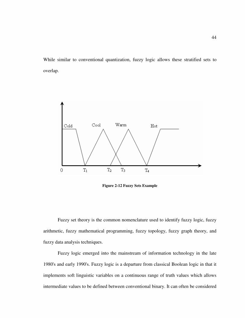
Fuzzy logic applications are a critical component of representing linguistic

variables, where general terms such a "large," "medium," and "small" are each used to

capture a range of numerical values. This may be explained in detail by temperature

membership functions for translation of knowledge. The Figure 2-12 illustrates the

method to define the fuzzy parameters of cold, cool, warm and hot using temperatures Ti.

44

While similar to conventional quantization, fuzzy logic allows these stratified sets to

overlap.

Figure 2-12 Fuzzy Sets Example

Fuzzy set theory is the common nomenclature used to identify fuzzy logic, fuzzy

arithmetic, fuzzy mathematical programming, fuzzy topology, fuzzy graph theory, and

fuzzy data analysis techniques.

Fuzzy logic emerged into the mainstream of information technology in the late

1980's and early 1990's. Fuzzy logic is a departure from classical Boolean logic in that it

implements soft linguistic variables on a continuous range of truth values which allows

intermediate values to be defined between conventional binary. It can often be considered

45

a superset of Boolean or "crisp logic" in the way fuzzy set theory is a superset of

conventional set theory.

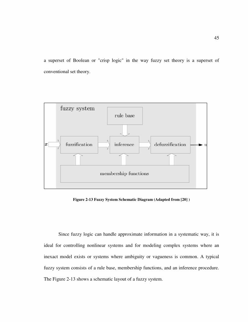
Figure 2-13 Fuzzy System Schematic Diagram (Adapted from [20] )

Since fuzzy logic can handle approximate information in a systematic way, it is

ideal for controlling nonlinear systems and for modeling complex systems where an

inexact model exists or systems where ambiguity or vagueness is common. A typical

fuzzy system consists of a rule base, membership functions, and an inference procedure.

The Figure 2-13 shows a schematic layout of a fuzzy system.

46

CHAPTER 3. METHODOLOGY

The work of Weckman et al [40] was extended to test if the performance of Neural

Network based forecasting model could be improved by increasing its knowledge

domain. This chapter describes the implementation of a Neural Network model in a

stock market scenario and the application of indicator pruning techniques and Elliot’s

wave theory. The primary objective of this research is to generate a one-day forecast of

the closing price using the techniques mentioned.

3.1 Stock Market Data

The stock market data used in this research was derived from various sources on

the World Wide Web, most notably, the financial websites maintained by Yahoo Inc. The

Dow Jones Global Classification Standard (DJGCS) � which comprised of economic

sectors, market sectors, industry groups and subgroups � provides correct and

internationally accepted industry and sector classifications. The following are the broad

economic sectors that are taken into consideration by typical stock market investors.

1. Basic Materials [BSC]

2. Consumer, Cyclical [CYC]

3. Energy [ENE]

4. Financial [FIN]

47

5. Healthcare [HCR]

6. Industrial [IDU]

7. Investment Products [IVP]

8. Consumer, Non-Cyclical [NCY]

9. Technology [TEC]

10. Telecommunications [TLS]

11. Utilities [UTI]

Stock selections for a typical investor are from different sectors of the stock

market so as to minimize risk in investment. Also, stocks chosen in an investment

portfolio have a mixture of growth and value stocks, thereby diversifying the portfolio

and minimizing risk while increasing long term returns. The stocks listed in Table 3-1

Stocks Analyzedwere the stocks selected and analyzed in this research.

48

Sector Ticker Symbol Name

Financial [FIN] BAC Bank of America Corp Financial [FIN] JPM JP Morgan Chase & Co. Financial [FIN] WB Wachovia Corporation

Technology [TEC] EMC EMC corporation Technology [TEC] HPQ HP Corporation Technology [TEC] STX Seagate Technologies Healthcare [HCR] RHB RehabCare Healthcare [HCR] AGP AmeriGroup Corporation Healthcare [HCR] WLP Well Point Inc.

Consumer Non-Cyclical [NCY] AMR AMR Corporation Consumer Non-Cyclical [NCY] CAL Continental Airlines Consumer Non-Cyclical [NCY] DAL Delta Airlines

Industrial [IDU] F Ford Motors Corporation Industrial [IDU] GM General Motors Corporation Industrial [IDU] HMC Honda Motor Corporation

Table 3-1 Stocks Analyzed

Preliminary data analysis is then performed and consists of identifying stock splits

and adjusting the value of the stocks. Hence the data used for the different stocks consists

of different time periods with the over lapping time periods are identified.

49

3.2 Analysis of Preliminary Indicators

The research starts with the development of a base line forecasting model based on

research published by Weckman et al [1][40]. Accordingly the preliminary model

developed was a Generalized Feed Forward network that has the following properties.

1. Input Processing Elements = 8

2. Hidden Layers: one layer containing 4 processing elements

3. Output Processing Elements = 1 (Closing Sales Price)

4. PE Transfer Function = TanhAxon

5. Maximum Number of Epochs = 5000

This model applied the stocks listed in Table 3-1 and the results form the baseline

performance against which further models are compared. The GFF network as

represented by NeuroSolutions is shown in Figure 3-1.

Figure 3-1 Generalized Feed Forward Network as represented by NeuroSolutions

50

The data required for analysis is compiled using spreadsheet management software,

Microsoft Excel, which is then used by NeuroSolutions.

3.3 Indicator Selection Using Self Organizing Map

This process is performed to identify new indicators that provide more information to

a Neural Network training algorithm, thereby aiding improvement in forecast generated.

Indicators are classified into the following categories:

1. Market Momentum Indicators

2. Market volatility Indicators

3. Market Trend Indicators

4. Broad Market Indicators

5. General Momentum Indicators

A total of 56 commonly used indicators are selected and they are listed in Table

3-2 as follows

51

Accumulation/Distribution Williams' Accumulation/Distribution Average Directional Movement Average True Range

Chaikin Oscillator Average True Range Band (Bottom) Commodity Channel Index Average True Range Band (Top)

Commodity Channel Index (General) Beta Directional Movement Index Beta On Decrease Directional Movement Rating Beta On Increase

Ease of Movement Bollinger Band (Bottom) Herrick Payoff Index Bollinger Band (Top)

Minus Directional Indicator Chaikin's Volatility Money Flow Index Keltner Channel (Bottom)

Money Flow Index (General) Keltner Channel (Top) On Balance Volume Mass Index

Plus Directional Indicator Trading Band (Bottom) Price and Volume Trend Trading Band (Top)

QStick Indicator True Range Stochastic Oscillator Aroon Down

Williams' %R Aroon Up Velocity Value Oscillator

Market Facilitation Index Upside/Downside Ratio Negative Volume Index Acceleration Positive Volume Index MACD Time Series Forecast Momentum

Vertical Horizontal Filter Rate-of-Change Absolute Breadth Index Relative Momentum Index

Absolute Breadth Index (Percent) Relative Strength Index New Highs/Lows Ratio TRIX

New Highs-Lows Cumulative Open-10 TRIN

Table 3-2 Input Indicators to a Self Organizing Map Network

52

The indicators mentioned are fed as input to a self-organizing map Neural

Network. All Neural Networks that are implemented for this problem were developed

using NeuroSolutions, proprietary software of NeuroDimension Inc. The indicators are

decomposed based on their formulae and the presence or absence of a particular property

is noted.

Figure 3-2 NeuroSolutions Representation of a Self Organizing Map

The properties checked for are close, high, low, period and volume and are coded

in a binary fashion as shown in Table 3-3 SOM Indicators Coding Methodology. The

self-organizing map based on the presence or absence of the properties, as shown in

Figure 2-1, clusters the indicators. The clusters are then analyzed and indicators are

chosen that are the closest to the cluster center.

53

Indicators Close High Low Period Volume Accumulation/Distribution 1 1 1 0 1

Average Directional Movement 1 1 1 1 0 Chaikin Oscillator 1 1 1 0 1

Commodity Channel Index 1 1 1 1 0 Commodity Channel Index

(General) 1 0 0 1 0 Directional Movement Index 1 1 1 1 0 Directional Movement Rating 1 1 1 1 0

Ease of Movement 0 1 1 0 1 Herrick Payoff Index 0 1 1 0 1

Table 3-3 SOM Indicators Coding Methodology

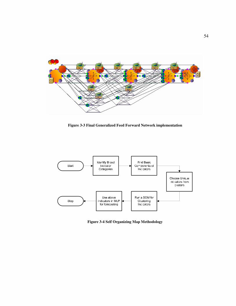
The values for the chosen indicators are then calculated for of the all the stock

market data. These are the inputs to the Generalized Feed Forward network as indicated

in Figure 3-3. This network was trained multiple times with 10,000 epochs for each run.

The best weights after cross validation was saved. The testing data was run over the

network with the saved weights and the results were noted. This methodology may be

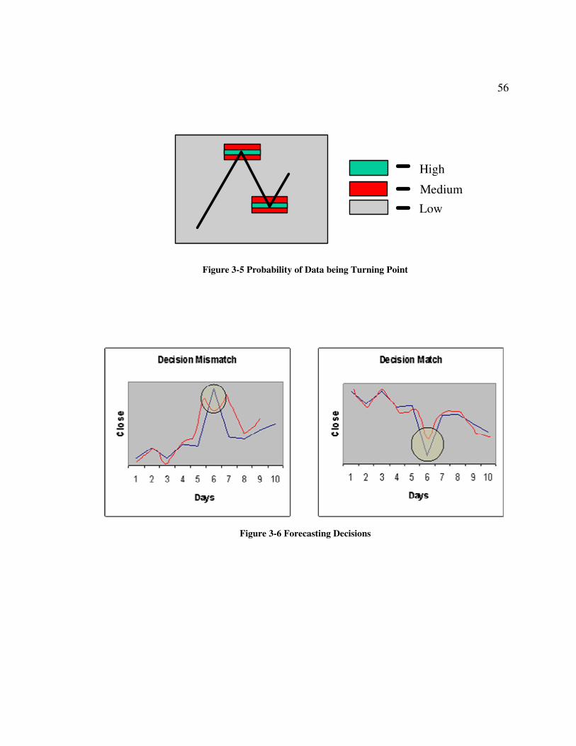
depicted as a flow of operations as shown in Figure 3-4.

54

Figure 3-3 Final Generalized Feed Forward Network implementation

Figure 3-4 Self Organizing Map Methodology

55

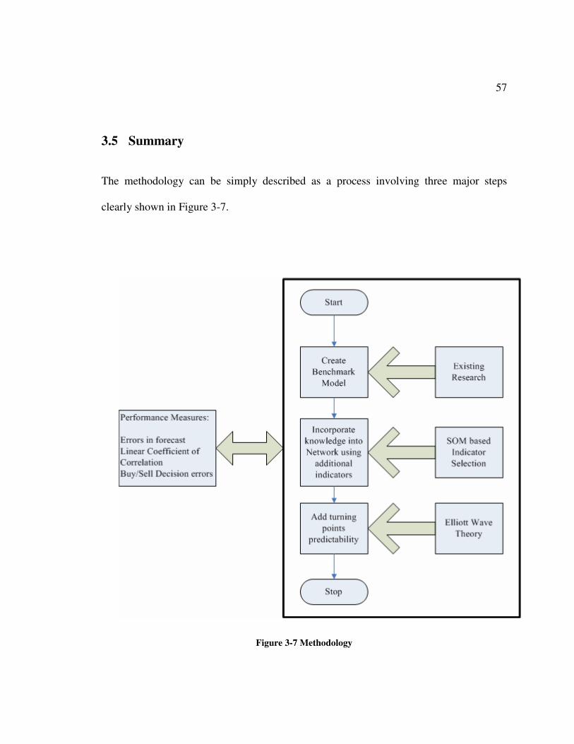
3.4 Elliott Wave Implementation

In a real life continuous data set, a definitive threshold cannot be established, but

each data point does have a certain degree of membership to a belief function [6] [39].

This concept is used to define the membership of Elliott Wave points in the current data

set. A Fibonacci Ratio based percentage is calculated for a given data set and the

membership functions for the Elliott Wave indicators are defined. The Elliott Wave and

the turning point indicators are found to inculcate a wavy nature in the output that scaled

the peaks and troughs of the actual wave. This helps immensely in the forecast of the

short term direction of the price movement. A decision match is nothing but forecasting

the right direction of movement of the price regardless of the magnitude. This concept is

explained graphically in Figure 3-6 . Thus the decision mismatches reduced in the

forecasting of a time series such as the stock market. Three fuzzy classes of high,

medium and low are set indicating the probability of the point being an Elliott Turning

Point (Figure 3-5). The fuzzy classes used are rectangular binding functions. The area

depicts the probability of that point being an Elliott Turning Point.

56

Medium

High

Low

Figure 3-5 Probability of Data being Turning Point

Figure 3-6 Forecasting Decisions

57

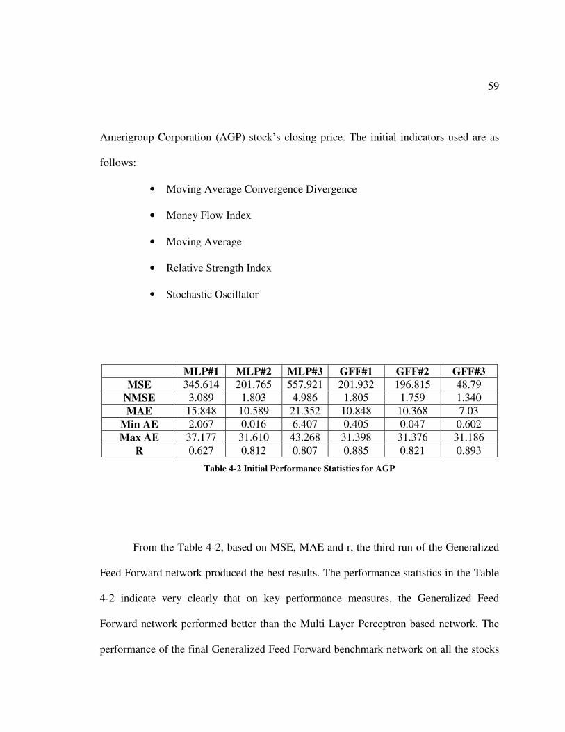
3.5 Summary

The methodology can be simply described as a process involving three major steps

clearly shown in Figure 3-7.

Figure 3-7 Methodology

58

CHAPTER 4. RESULTS AND DISCUSSION

4.1 Performance of the Benchmark Network

The benchmark network was selected based on the results and principles of

network selection by Weckman et al [40]. Different network architectures using a

multitude of factors were tested for the performance measures listed in Table 4-1

Performance Measures Abbreviations Mean Squared Error MSE

Normalized Mean Squared Error NMSE Mean Absolute Error MAE

Minimum Absolute Error MinAE Maximum Absolute Error MaxAE

Linear Correlation Coefficient r

Table 4-1 Performance Measures

The architectures that were tested are the Generalized Feed Forward and

Multilayer Perceptrons. Different networks were constructed using different parameters.

The parameters that were modified are the number of Perceptrons, number of layers, the

step size and the method of weight update. The Table 4-2 indicates the results for the 3

different Multilayer Perceptrons and Generalized Feed Forward networks on the

59

Amerigroup Corporation (AGP) stock’s closing price. The initial indicators used are as

follows:

• Moving Average Convergence Divergence

• Money Flow Index

• Moving Average

• Relative Strength Index

• Stochastic Oscillator

MLP#1 MLP#2 MLP#3 GFF#1 GFF#2 GFF#3 MSE 345.614 201.765 557.921 201.932 196.815 48.79

NMSE 3.089 1.803 4.986 1.805 1.759 1.340 MAE 15.848 10.589 21.352 10.848 10.368 7.03

Min AE 2.067 0.016 6.407 0.405 0.047 0.602 Max AE 37.177 31.610 43.268 31.398 31.376 31.186

R 0.627 0.812 0.807 0.885 0.821 0.893

Table 4-2 Initial Performance Statistics for AGP

From the Table 4-2, based on MSE, MAE and r, the third run of the Generalized

Feed Forward network produced the best results. The performance statistics in the Table

4-2 indicate very clearly that on key performance measures, the Generalized Feed

Forward network performed better than the Multi Layer Perceptron based network. The

performance of the final Generalized Feed Forward benchmark network on all the stocks

60

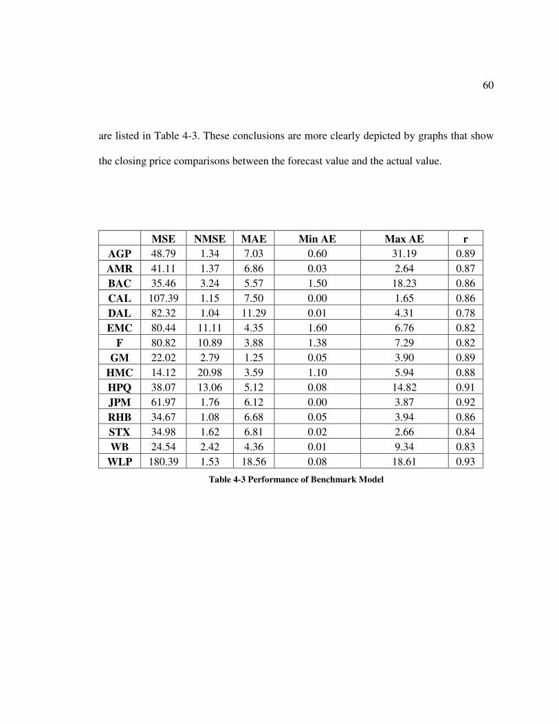
are listed in Table 4-3. These conclusions are more clearly depicted by graphs that show

the closing price comparisons between the forecast value and the actual value.

MSE NMSE MAE Min AE Max AE r AGP 48.79 1.34 7.03 0.60 31.19 0.89 AMR 41.11 1.37 6.86 0.03 2.64 0.87 BAC 35.46 3.24 5.57 1.50 18.23 0.86 CAL 107.39 1.15 7.50 0.00 1.65 0.86 DAL 82.32 1.04 11.29 0.01 4.31 0.78 EMC 80.44 11.11 4.35 1.60 6.76 0.82

F 80.82 10.89 3.88 1.38 7.29 0.82 GM 22.02 2.79 1.25 0.05 3.90 0.89

HMC 14.12 20.98 3.59 1.10 5.94 0.88 HPQ 38.07 13.06 5.12 0.08 14.82 0.91 JPM 61.97 1.76 6.12 0.00 3.87 0.92 RHB 34.67 1.08 6.68 0.05 3.94 0.86 STX 34.98 1.62 6.81 0.02 2.66 0.84 WB 24.54 2.42 4.36 0.01 9.34 0.83

WLP 180.39 1.53 18.56 0.08 18.61 0.93

Table 4-3 Performance of Benchmark Model

61

0

10

20

30

40

50

60

70

80

90

1 16 31 46 61 76 91 106 121 136 151

Days

Clo

sing

Pri

ce

Actual Forecast

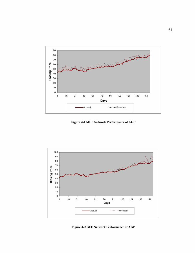
Figure 4-1 MLP Network Performance of AGP

0

10

20

30

40

50

60

70

80

90

100

1 16 31 46 61 76 91 106 121 136 151

Days

Clo

sing

Pri

ce

Actual Forecast

Figure 4-2 GFF Network Performance of AGP

62

The Figure 4-1 and Figure 4-2 show the graphs of the actual closing price and the

forecasted closing price. The Figure 4-2 shows the performance of Generalized Feed

Forward which is superior to Figure 4-1 showing the performance of a Multilayer

Perceptron. Figure 4-2 also indicates that the predicted close values follow the actual

close values more closely. Similar results were obtained for all the remaining stock

prices.

Figure 4-3 Distribution of Actual vs. Predicted Close of AGP

63

4.2 Indicator Analysis using Self Organizing Maps

The performance of the benchmark network developed in the previous section had the

following short comings due to the limitations of the 5 indicators used for input:

• High Mean Squared Error (MSE)

• Low linear correlation coefficient (r)

• Poor forecasting results in unknown scenarios

These shortcomings can be overcome by providing the selected Generalized Feed

Forward network with more information on trend, momentum and volatility of the

closing price. This information can be supplied to the network using a variety of

indicators. All the indicators cannot be provided to the network, due to the fact that the

network becomes too complex and the evaluation time increases by a magnitude of 10.

Therefore indicators representative of a particular information property have to be

selected. This is carried out by coding the indicators based on their constituents in the

formula. The following is the formula for the Ease of Movement indicator.

tt

tttt

LowHighVolume

LowHighLowHighMA

EoM

−

+−

+

=−− )}

2()

2{( 21

Where

• EoM = Ease of Movement

• MA = Moving Average

64

It is clear from the above formula that the Ease of Movement indicator utilizes the

High, Low and Volume of the stock. Thus the columns High, Low and Volume receive a

1 during Self Organizing Map coding and all other fields receive a 0. A sample of this

coded input is shown in Table 4-4.

Indicators Close High Low Period Volume Accumulation/Distribution 1 1 1 0 1

Average Directional Movement 1 1 1 1 0 Chaikin Oscillator 1 1 1 0 1

Commodity Channel Index 1 1 1 1 0 Commodity Channel Index

(General) 1 0 0 1 0 Directional Movement Index 1 1 1 1 0 Directional Movement Rating 1 1 1 1 0

Ease of Movement 0 1 1 0 1 Herrick Payoff Index 0 1 1 0 1

Minus Directional Indicator 1 1 1 1 0

Table 4-4 SOM Indicators Coding Methodology

65

The self organizing map suggested the use of the indicators listed in Table 4-5 to

generalize the knowledge provided by various indicators.

Type of Indicator Name Market Momentum Indicators Money Flow Index

Chaikin Oscillator Williams %R

Market Volatility Indicators Mass Index Bollinger Band Trading Band (top)

Market Trend Indicators Aroon Down Aroon Up

Broad Market Indicators STIX General Momentum Indicators TRIX

Relative Momentum Index

Table 4-5 SOM Indicators

These indicators are calculated for the closing price of all stocks. The period used

in the calculation of all the indicators, where period is required as an input, is ten days

which roughly translates into two business weeks.

These inputs derived from the self organizing map were then provided to the

Generalized Feed Forward network selected in Table 4-2 for further enhancement of the

models. The results of this model are listed in Table 4-6. The model was tested on data

from the Amerigroup Corporation stock prices for comparison purposes.

66

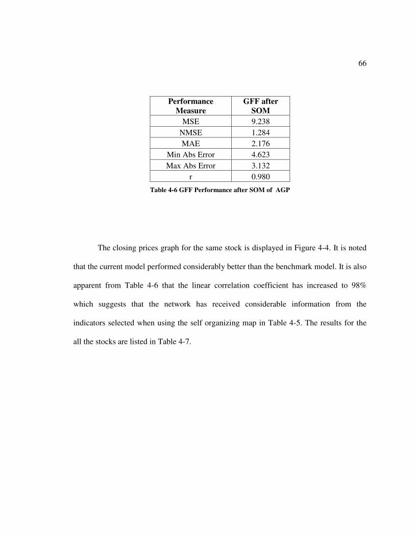
Performance Measure

GFF after SOM

MSE 9.238 NMSE 1.284 MAE 2.176

Min Abs Error 4.623 Max Abs Error 3.132

r 0.980

Table 4-6 GFF Performance after SOM of AGP

The closing prices graph for the same stock is displayed in Figure 4-4. It is noted

that the current model performed considerably better than the benchmark model. It is also

apparent from Table 4-6 that the linear correlation coefficient has increased to 98%

which suggests that the network has received considerable information from the

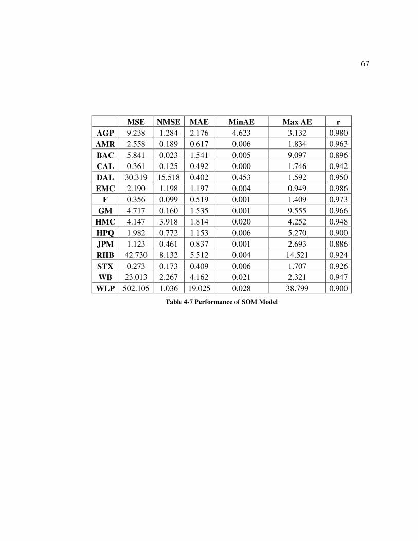
indicators selected when using the self organizing map in Table 4-5. The results for the

all the stocks are listed in Table 4-7.

67

MSE NMSE MAE MinAE Max AE r AGP 9.238 1.284 2.176 4.623 3.132 0.980 AMR 2.558 0.189 0.617 0.006 1.834 0.963 BAC 5.841 0.023 1.541 0.005 9.097 0.896 CAL 0.361 0.125 0.492 0.000 1.746 0.942 DAL 30.319 15.518 0.402 0.453 1.592 0.950 EMC 2.190 1.198 1.197 0.004 0.949 0.986

F 0.356 0.099 0.519 0.001 1.409 0.973 GM 4.717 0.160 1.535 0.001 9.555 0.966


WLP 502.105 1.036 19.025 0.028 38.799 0.900

Table 4-7 Performance of SOM Model

68

0

10

20

30

40

50

60

70

80

90

1 16 31 46 61 76 91 106 121 136 151

Days

Clo

sing

Pri

ce

Actual Forecast

Figure 4-4 GFF with SOM Indicators Output

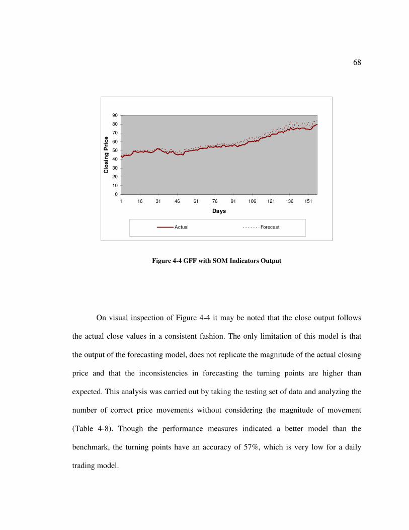
On visual inspection of Figure 4-4 it may be noted that the close output follows

the actual close values in a consistent fashion. The only limitation of this model is that

the output of the forecasting model, does not replicate the magnitude of the actual closing

price and that the inconsistencies in forecasting the turning points are higher than

expected. This analysis was carried out by taking the testing set of data and analyzing the

number of correct price movements without considering the magnitude of movement

(Table 4-8). Though the performance measures indicated a better model than the

benchmark, the turning points have an accuracy of 57%, which is very low for a daily

trading model.

69

Number of Testing Data Points 158 Number of correct change predictions 90 Number of incorrect change predictions 68 Percentage Accuracy 56.96%

Table 4-8 Price Movement Prediction Results

4.3 Elliott Wave Indicators Implementation

The performance of the network developed in the previous section had the following

shortcomings:

• High Mean Squared Error (MSE)

• High Max and Min Absolute Error (Min Abs Error, Max Abs Error)

• Low percentage of accuracy in prediction of turning points.

These shortcomings were dealt with by developing two indicators based on the Elliott

Wave principle. The first indicator uses the basic tenets of Elliott Wave discussed in

Section 2.2 to develop a turning point indicator called the Elliott Wave Turning point

Indicator (EWTP). The second indicator provides the magnitude information using Elliott

Wave principles and is called the Elliott Wave Magnitude Indicator (EWM). The

performance of this network is shown in Figure 4-5, Figure 4-66 and Table 4-9. The final

networks performance on all the stocks is listed in Table 4-10.

70

Performance Measure Final Network Properties MSE 5.370

NMSE 0.867 MAE 6.806

Min AE 0.028 Max AE 2.613

r 0.996

Table 4-9 Final Network Performance

MSE NMSE MAE Min AE Max AE r AGP 5.370 0.867 6.806 0.028 2.613 0.996 AMR 0.537 0.182 0.604 0.017 1.948 0.966 BAC 4.257 0.017 1.356 0.003 6.673 0.998 CAL 5.828 2.022 0.201 0.050 0.431 0.999 DAL 3.568 1.812 1.409 0.003 4.213 0.983 EMC 1.955 3.717 1.181 0.071 5.065 0.998

F 1.418 0.113 0.503 0.115 1.028 0.991 GM 3.752 0.128 1.459 0.016 6.842 0.961


WLP 1.512 0.973 1.228 0.100 0.636 0.939

Table 4-10 Final Network Performance

71

0

10

20

30

40

50

60

70

80

90

100

1 16 31 46 61 76 91 106 121 136 151

Days

Clo

sing

Pri

ce

Actual Forecast

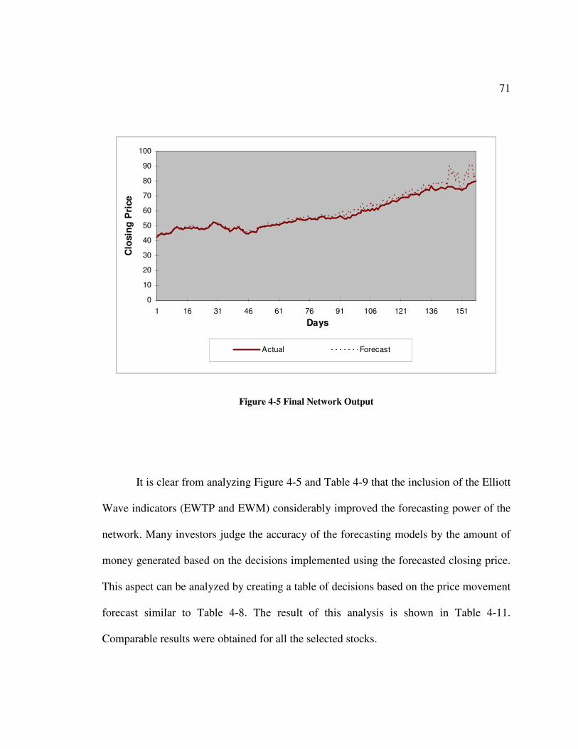
Figure 4-5 Final Network Output

It is clear from analyzing Figure 4-5 and Table 4-9 that the inclusion of the Elliott

Wave indicators (EWTP and EWM) considerably improved the forecasting power of the

network. Many investors judge the accuracy of the forecasting models by the amount of

money generated based on the decisions implemented using the forecasted closing price.

This aspect can be analyzed by creating a table of decisions based on the price movement

forecast similar to Table 4-8. The result of this analysis is shown in Table 4-11.

Comparable results were obtained for all the selected stocks.

72

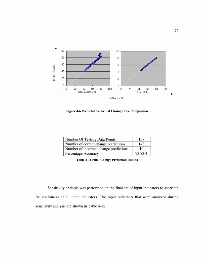
Figure 4-6 Predicted vs. Actual Closing Price Comparison

Number Of Testing Data Points 158 Number of correct change predictions 148 Number of incorrect change predictions 10 Percentage Accuracy 93.83%

Table 4-11 Final Change Prediction Results

Sensitivity analysis was performed on the final set of input indicators to ascertain

the usefulness of all input indicators. The input indicators that were analyzed during

sensitivity analysis are shown in Table 4-12.

73

Indicator Name Symbol Aroon Down Aroon Down

Aroon Up Aroon Up Bollinger Band BB(Bottom)

Chaikin Oscillator CO Moving Average Convergence Divergence MACD

Mass Index Mass Index Money Flow Index MFI Moving Average M Avg

Relative Momentum Index RMI Relative Strength Index RSI

STIX Indicator STIX Stochastic Oscillator SO Trading Band (Top) Tband(Top)

TRIX Indicator TRIX Williams' %R Williams' %R

Elliott Wave turning point EWTP Elliott Wave magnitude EWM

Table 4-12 Indicators used in Sensitivity Analysis

The following is the sensitivity analysis performed by varying inputs over two

standard deviation lengths of the mean. The Figure 4-7 shows the resulting graph. The

graph was truncated at a sensitivity value of 0.02, to exaggerate and clearly show the

effect of some low sensitivity indicators.

74

00.0020.0040.0060.008

0.010.0120.0140.0160.018

0.02

Aroon

Dow

n

Aroon U

p

BB

(Bottom

)

CO

MA

CD

Mass Index

MFI

M A

vg

RM

I

RSI

STIX

SO Tband(T

op)

TR

IX

William

s'%

R

EW

TP

EW

M

Input Name

Sens

itivi

ty

Figure 4-7 Relative Sensitivity of Indicators

It is obvious from the indicator analysis graph that all inputs except the Chaikin

Oscillator have an impact on the output closing price. Even though the indicators Aroon

Up and Aroon Down have low sensitivity on the output, they play a key role in providing

consistent information to the network. This aspect was tested by removing the indicators

with low sensitivity, but the resultant model had a marked decrease in the major

performance factors. Thus all indicators selected with the exception of the Chaikin

Oscillator played a pivotal role in the forecasting accuracy of the final model generated.

75

CHAPTER 5. CONCLUSIONS AND FUTURE RESEARCH

5.1 Conclusions

The thesis presents a novel and integrated approach to the problem of stock

market forecasting. Stock markets are considered to be one of the most complex time

series to model. This is due to the fact that stock markets have numerous underlying

factors, most of which are currently not fully understood. Technical analysis of the stock

market is a technique that does not require a thorough understanding of component

factors. This concept can be utilized on a machine learning system such as an Artificial

Neural Network, to understand the behavior of the stocks.

Initially a benchmark Neural Network was designed based on the published work

of Weckman et al. [1][40]. In the process of developing the optimal benchmark, different

network properties and architectures were tested. The optimal network was selected

based on a set of performance measures. This network was tested on various stocks as

listed in Table 3-1 to ensure the portability of the model across a spectrum of stocks.

The performance of this network was lacking in forecasting accuracy. More indicators

were needed to impart the required knowledge for improving the performance of the

network. Researchers and stock market analysts have historically used a large amount of

indicators that have yielded very good results in different regimes of the financial market.

76

All indicators cannot be applied to a Neural Network, due to computing power and

network complexity considerations. Therefore a unique method was devised to select a

set of indicators that were representative of the genre of indicators. A Self Organizing

Map was used to select networks based on their constituent properties.

These indicators were calculated for all the stocks and network analysis was

performed to this improved network. The results were confirmed to improve the accuracy

of forecasting by a significant amount. The network was still found to be lacking in

forecasting turning points and magnitudes for new scenarios.

The Elliott Wave Theory possesses empirical rules that utilize the omni present

principle of Fibonacci ratios and the Golden Ratio. These principles have been

successfully used by traders to generate very accurate forecasts of the stock market.

These principles were coded in the form of two indicators, namely the Elliott Wave

turning point and the Elliott Wave magnitude indicators. This information aided the

network’s learning process thereby increasing the accuracy of the forecast both in terms

of magnitude and direction.

In summary this research was able generate a final comprehensive stock market

forecasting model by successively improving the Benchmark model by incorporating

different techniques in a sequential fashion.

77

5.2 Future Research

This research focused primarily on developing a comprehensive Neural Network

model for forecasting stock markets. There is an unambiguous scope for enhancement in

the current research along the following directions.

Rule Extraction

The Neural Network stores knowledge gained during training in the form of

connection weights or synapses. The knowledge gained by the network cannot be

compared to the financial theories of the stock market. To draw this parallel of analysis,

simple rules can be extracted from the model to corroborate the learning of the model

with financial theories. This can lead to the development of a network that is based on

sound financial principles.

Knowledge-Based Neurocomputing

An important consideration in the development of a Neural Networks is the time

and cost of training. Knowledge-primed or hint-based training strategies can be used to

considerably enhance the training routine. These procedures map the architecture of the

Neural Network to the available domain knowledge. This significantly reduces the

complexity of the training process. The process is also known to increase prediction

accuracies.

78

Long-Term Forecasting

The proposed model is constructed by training the network on significantly large

amounts of data to develop the forecast of the subsequent period. This may not be a

financially attractive proposition because of the compounding nature of the errors.

Therefore a long-term forecasting model would need to be generated to assess the

performance of the model in a real-life investment situation.

Scalability

The research focuses on short term forecasting methodology of Stock Markets.

Though the research cannot be directly extended to solve problems with other examples

of noisy Time Series data, the model can be modified to suit a variety of applications.

The processes involved in the course of this research can be scaled to other vertical

applications such as demand forecasting and production planning.

Incorporating Low Probability Events

The research assumes that the underlying processes governing the stock market

price movements are constant. The model may be improved by providing knowledge for

incorporating low probability events such as a natural disaster.

79

REFERENCES

[1] Agarwala, R., Weckman, G. R., and McLauchlan, R., “Optimization of Data Collection and Training Time for Forecasting Stock Market Trends Using Artificial Neural Network”, Proceedings of the 2002 Artificial Neural Networks in Engineering Conference, pp. 707-712, 2002.

[2] Almeida, L., “A Learning Rule in Perceptrons with Feedback in a Combinatorial Environment.”, 1st IEEE International Conference in Neural Networks, pp. 609-618, 1987.

[3] Anderson, J., and Rosenfeld, E., “NeuroComputing: Foundations for Research.” MIT Press, 1990.

[4] Baba, N., and Kozaki, M., “An Intelligent Forecasting System of Stock Price using Neural Networks”, Proceedings of the International Joint conference on Neural Networks, Vol. 1, pp. 371-377, 1992.

[5] Baldi, P., “Gradient Descent Learning Algorithms Overview: A General Dynamical Systems Perspective”, IEEE Transactions on Neural Networks, Vol. 6, pp. 182-195, 1995.

[6] Bogullu, V.K., Enke, D., and Dagli, C., “Using Neural Networks and Technical Indicators for Generating Stock Trading Signals”, Proceedings of the 2002 Artificial Neural Networks in Engineering Conference, pp. 721-726, 2002.

[7] Caianiello, E., “Outline of a Theory of Thought-Processes and Thinking Machines.”, Journal of Theoretical Biology, pp. 204-235, 1961.

[8] Elman, J., “Finding Structure in Time”, Cognitive Science 14, pp. 179-211, 1990.

[9] Gately, E., “Neural Networks for Financial Forecasting”, New York, Wiley, 1996.

[10] Hadik, E. S., “Fibonacci Squared”, Futures, 28 (7), pp. 38-42, July 1999. [11] Holter, J.T., “The Markets' Hidden Order”, Futures, 25 (13), pp. 66-71,

November 1997. [12] Hopfield, J., “Neural Networks and Physical Systems with Emergent Collective

Computational Abilities.”, Proceedings of the National Academy of Science, pp. 2554-2558, 1982.

[13] “Elliott Wave Theory, General and Basic Theory”. Retrieved October 13, 2005, from http://www.Elliott-wave-theory.com.

[14] Jang, G., Lai, F., and Parng, T., “Intelligent Stock Trading Decision Support System using Dual Adaptive-Structure Neural Networks”, Journal of Information Science and Engineering, pp. 271-297, June 1993.

80

[15] Kimoto T., Asakawa K. Y. and Takeoka M., “Stock Market Prediction System with Modular Neural Network”, Proceedings of the International Joint Conference on Neural Networks, San Diego, California, pp. 1-6, 1990.

[16] Kohara, I., and Fukuhara, N., “Stock Price Prediction using Prior Knowledge and Neural Networks”, International Journal of Intelligent Systems in Accounting, Finance and Management, 6 (1), pp. 11-22, 1997.

[17] Kohonen T. “The Self Organizing Map” Proceedings of IEEE 78, pp. 1464-1480, 1990.

[18] Kohonen, T., Self Organization Maps, New York: Springer-Verlag, 1997. [19] Kohonen, T., Self Organization and Associative Memory, New York: Springer-

Verlag, 1988. [20] Kosko, B., Neural Networks and Fuzzy Systems. Prentice Hall, 1992. [21] Kung S.Y., Digital Neural Networks. Prentice Hall, 1993. [22] Kyoung-jae, K., and Ingoo, H.,”Genetic Algorithms Approach to Feature

Discretization in Artificial Neural Networks for the Prediction of Stock Price Index”, Expert System with Applications, 19 (2), pp. 125-132, 2000.

[23] Lee, K. H., and Jo, G. S., “Expert System for Predicting Stock Market Timing using Candlestick Chart”, Expert Systems with Applications, 16, pp. 357-364, 1999.

[24] Lippman, R., “An Introduction to Computing with Neural Nets”, IEEE Transactions - ASSP Magazine 4, 4-22, 1987.

[25] Makhoul, J., “Pattern Recognition Properties of Neural Networks”, Proceedings of the 1991 IEEE Workshop on Neural Networks for Signal Processing, pp 173-187, 1992.

[26] Minsky, M., and Papert, S., Perceptrons. MIT Press, 1969. [27] Prechter Jr., .R.R., “R.N. Elliott's Masterworks: The Definitive Collection”,

New Classics Library, Georgia, 1994. [28] Rosenblatt, F., “The Perceptron: a Probabilistic Model for Information Storage

and Organization in the Brain”, Physiological Review 65, 386-408, 1958. [29] Rumelhart D., Hinton G., and Williams R., “Learning Internal Representations

by Error Propagation”, Parallel Distributed Processing, MIT Press, 1986. [30] Saad, E. W., Prokhorov, D.V., and Wunsch, D. C., “Comparative study of

Stock Trend Prediction using Time Delay, Recurrent and Probabilistic Neural Networks”, IEEE Transactions on Neural Networks, Vol. 9, No. 6, pp. 1456-1470, 1998.

[31] Sanger, T., “Optimal Unsupervised Learning in a Single Layer Linear Feed Forward Network”, Neural Networks 12, 459-473, 1989.

[32] Schoenburg, E., "Stock Price Prediction using Neural Networks", Neurocomputing, 2, pp. 1409-1418, 1990.

[33] Shadbolt, J., and Taylor, J.G., Neural Networks and the Financial Markets: Predicting, Combining and Portfolio Optimization, Springer, New York, 2002.

81

[34] Skapura, D.M., Building Neural Networks, Addison-Wesley, New York, 1996. [35] Smith, K.A., and Gupta, J.N.D., "Neural Networks in Business: Techniques

and Applications for the Operations Researcher", Computers and Operations Research, 27, pp. 1023-1044, 2000.

[36] Strand, S., "Forecasting the Future: Pitfalls in Controlling for Uncertainty", Futures, 31, 333-350, 1999.

[37] Thawornwong, S., Enke, D., and Dagli, C., “Using Neural Networks and Technical Analysis Indicators for Predicting Stock Trends”, Proceedings of the 2001 Artificial Neural Networks in Engineering Conference (ANNIE '01), ASME, St. Louis, Missouri, 2001.

[38] Thrun, S., and Smieja, F., “A General Feed Forward Algorithm for Gradient Descent Learning in Connectionist Networks”, German National Research Center for Computer Science., 1991.

[39] Turban, E., and Aronson, J.E., Decision Support Systems and Intelligent Systems, Sixth Edition, Prentice Hall, New Jersey, 2001.

[40] Weckman, G.R., and Agarwala, R., “Identifying Relative Contribution of Selected Technical Indicators in Stock Market Prediction”, Proceedings of the IIE Annual Conference 2002, May 18-21, Portland, Oregon, 2002.

[41] Yao, J., Li, Y., and Tan, C. L., “Option Price Forecasting using Neural Networks”, Omega, 28, pp. 455-466, 2000.

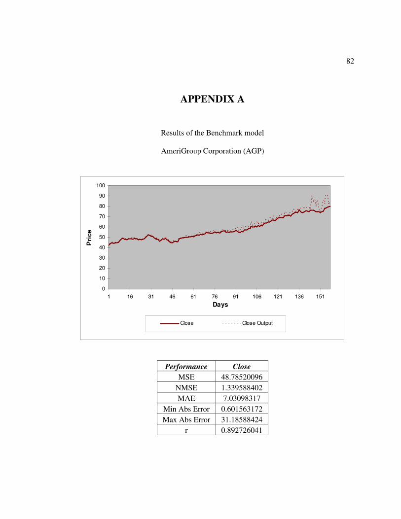
82

APPENDIX A

Results of the Benchmark model

AmeriGroup Corporation (AGP)

0

10

20

30

40

50

60

70

80

90

100

1 16 31 46 61 76 91 106 121 136 151Days

Pri

ce

Close Close Output

Performance Close MSE 48.78520096

NMSE 1.339588402 MAE 7.03098317


r 0.892726041

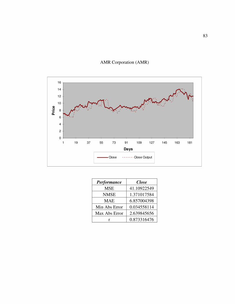
83

AMR Corporation (AMR)

0

2

4

6

8

10

12

14

16

1 19 37 55 73 91 109 127 145 163 181

Days

Pri

ce

Close Close Output


NMSE 1.371017584 MAE 6.857004398


r 0.873316476

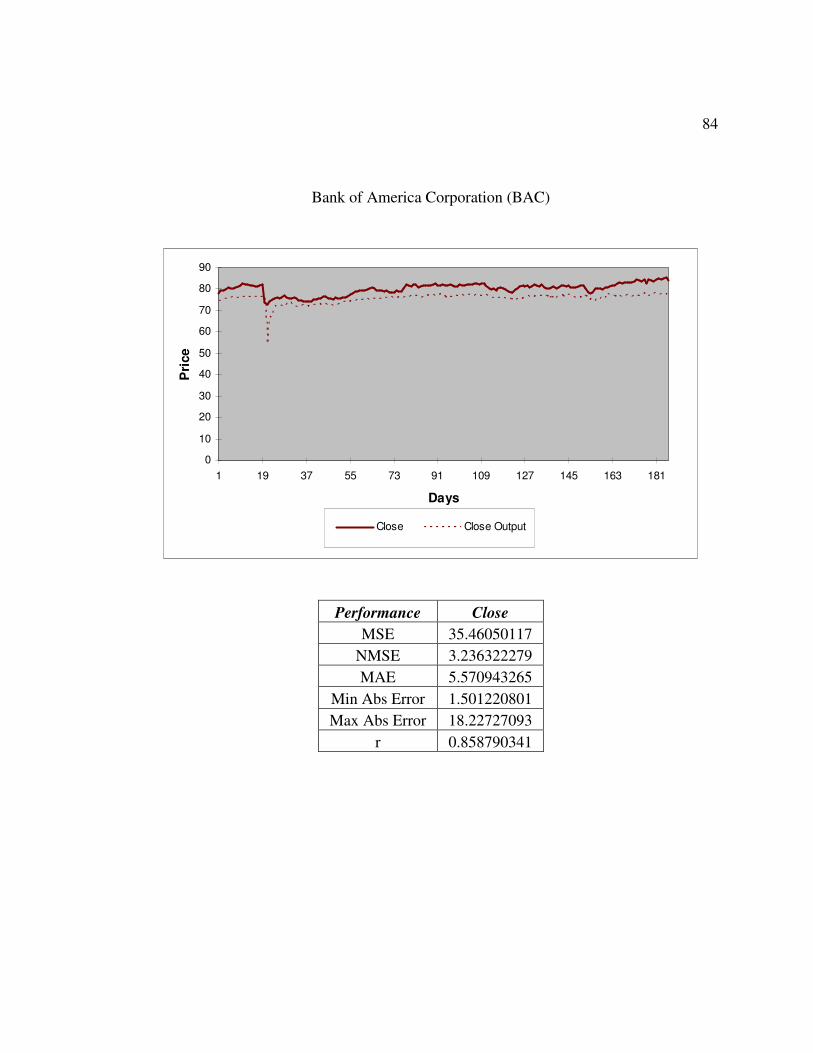
84

Bank of America Corporation (BAC)

0

10

20

30

40

50

60

70

80

90

1 19 37 55 73 91 109 127 145 163 181

Days

Pri

ce

Close Close Output


NMSE 3.236322279 MAE 5.570943265


r 0.858790341

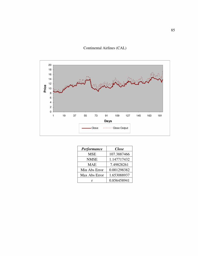
85

Continental Airlines (CAL)

0

2

4

6

8

10

12

14

16

18

20

1 19 37 55 73 91 109 127 145 163 181

Days

Pri

ce

Close Close Output


NMSE 1.147717432 MAE 7.49828261


r 0.856458941

86

Delta Airlines (DAL)

0

1

2

3

4

5

6

7

8

9

10

1 19 37 55 73 91 109 127 145 163 181

Days

Pri

ce

Close Close Output


NMSE 1.038127036 MAE 11.28951202


r 0.775779238

87

EMC Corporation (EMC)

0

2

4

6

8

10

12

14

16

18

1 19 37 55 73 91 109 127 145 163 181

Days

Pri

ce

Close Close Output


NMSE 11.11416048 MAE 4.34915939


r 0.823126495

88

Ford Corporation (F)

0

2

4

6

8

10

12

14

16

18

1 19 37 55 73 91 109 127 145 163 181

Days

Pri

ce

Close Close Output


NMSE 10.89355011 MAE 3.87865195


r 0.823156551

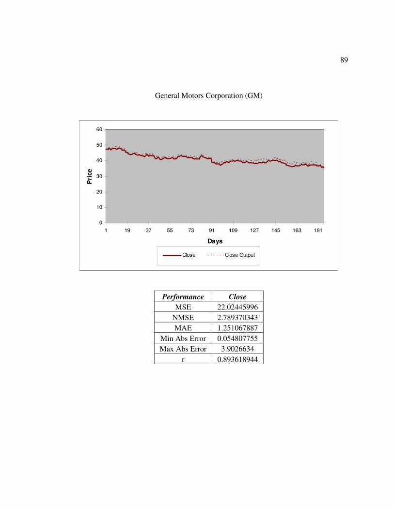
89

General Motors Corporation (GM)

0

10

20

30

40

50

60

1 19 37 55 73 91 109 127 145 163 181

Days

Pri

ce

Close Close Output


NMSE 2.789370343 MAE 1.251067887


r 0.893618944

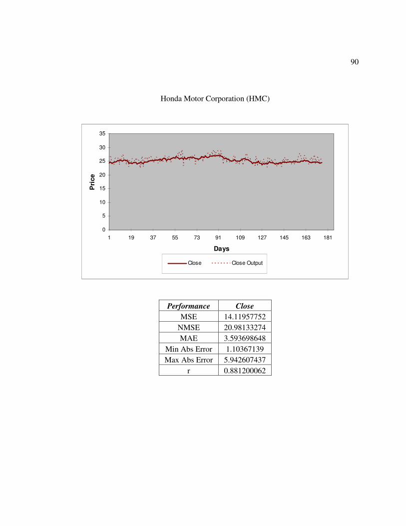
90

Honda Motor Corporation (HMC)

0

5

10

15

20

25

30

35

1 19 37 55 73 91 109 127 145 163 181

Days

Pri

ce

Close Close Output


NMSE 20.98133274 MAE 3.593698648


r 0.881200062

91

HP Corporation (HPQ)

0

5

10

15

20

25

1 19 37 55 73 91 109 127 145 163 181

Days

Pri

ce

Close Close Output


NMSE 13.05742419 MAE 5.122629976


r 0.910922065

92

JP Morgan Chase & Company (JPM)

0

5

10

15

20

25

30

35

40

45

1 19 37 55 73 91 109 127 145 163 181

Days

Pri

ce

Close Close Output


NMSE 1.759761763 MAE 6.116980307

Min Abs Error 9.96226E-05 Max Abs Error 3.866072744

r 0.916361288

93

RehabCare (RHB)

0

5

10

15

20

25

30

35

1 19 37 55 73 91 109 127 145 163 181

Days

Pri

ce

Close Close Output


NMSE 1.079563265 MAE 6.680116922


r 0.863385601

94

Seagate Technologies (STX)

0

5

10

15

20

25

1 19 37 55 73 91 109 127

Days

Pri

ce

Close Close Output


NMSE 1.615945403 MAE 6.806768738


r 0.836828011

95

Wachovia Corporation (WB)

0

10

20

30

40

50

60

1 19 37 55 73 91 109 127

Days

Pri

ce

Close Close Output


NMSE 2.417838073 MAE 4.360653732


r 0.832991243

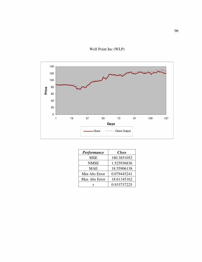
96

Well Point Inc (WLP)

0

20

40

60

80

100

120

140

1 19 37 55 73 91 109 127

Days

Pri

ce

Close Close Output


NMSE 1.525936836 MAE 18.55906138


r 0.933737225

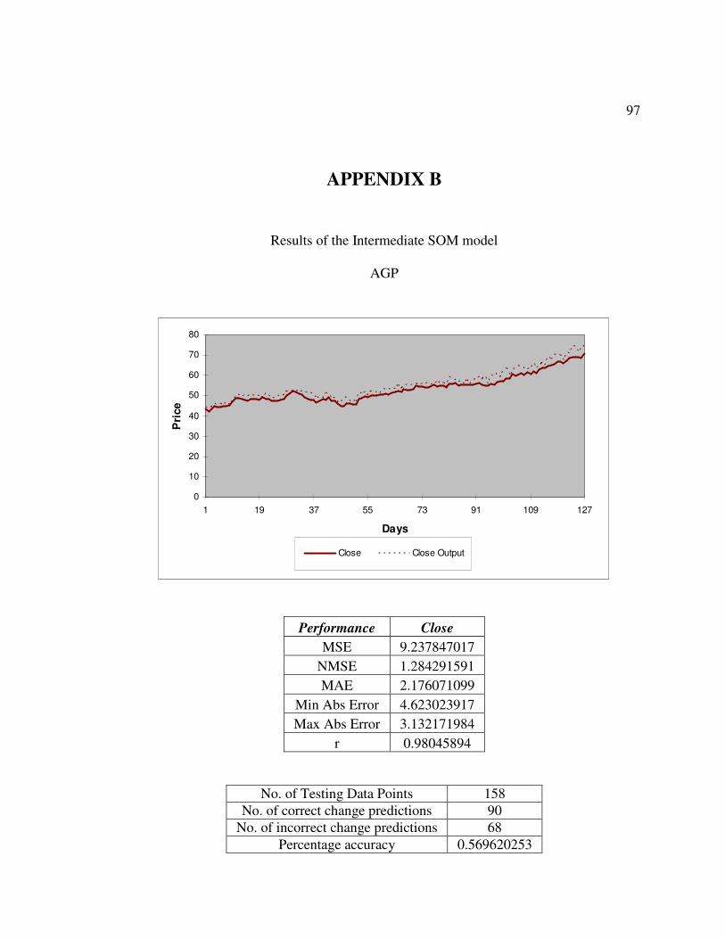
97

APPENDIX B

Results of the Intermediate SOM model

AGP

0

10

20

30

40

50

60

70

80

1 19 37 55 73 91 109 127

Days

Pri

ce

Close Close Output


NMSE 1.284291591 MAE 2.176071099


r 0.98045894

No. of Testing Data Points 158 No. of correct change predictions 90

No. of incorrect change predictions 68 Percentage accuracy 0.569620253

98

AMR

0

2

4

6

8

10

12

14

1 19 37 55 73 91 109 127

Days

Pri

ce

Close Close Output


NMSE 0.189051515 MAE 0.617245373


r 0.963475731


No. of incorrect change predictions 124 Percentage accuracy 54.57875%

99

BAC

0

10

20

30

40

50

60

70

80

90

100

1 19 37 55 73 91 109 127

Days

Pri

ce

Close Close Output


NMSE 0.022688254 MAE 1.540529363


r 0.896253842



100

CAL

0

2

4

6

8

10

12

14

1 19 37 55 73 91 109 127

Days

Pri

ce

Close Close Output


NMSE 0.125242984 MAE 0.491885186


r 0.941700748



101

DAL

0

1

2

3

4

5

6

7

8

9

1 19 37 55 73 91 109 127

Days

Pri

ce

Close Close Output


NMSE 15.51751531 MAE 0.401726698


r 0.950411876



102

EMC

0

2

4

6

8

10

12

14

16

18

1 19 37 55 73 91 109 127

Days

Pri

ce

Close Close Output


NMSE 1.198044251 MAE 1.196790291


r 0.985691312



103

F

0

2

4

6

8

10

12

14

16

18

1 19 37 55 73 91 109 127 145 163 181 199 217 235 253 271

Days

Pri

ce

Close Close Output


NMSE 0.098908304 MAE 0.519338063


r 0.972725318



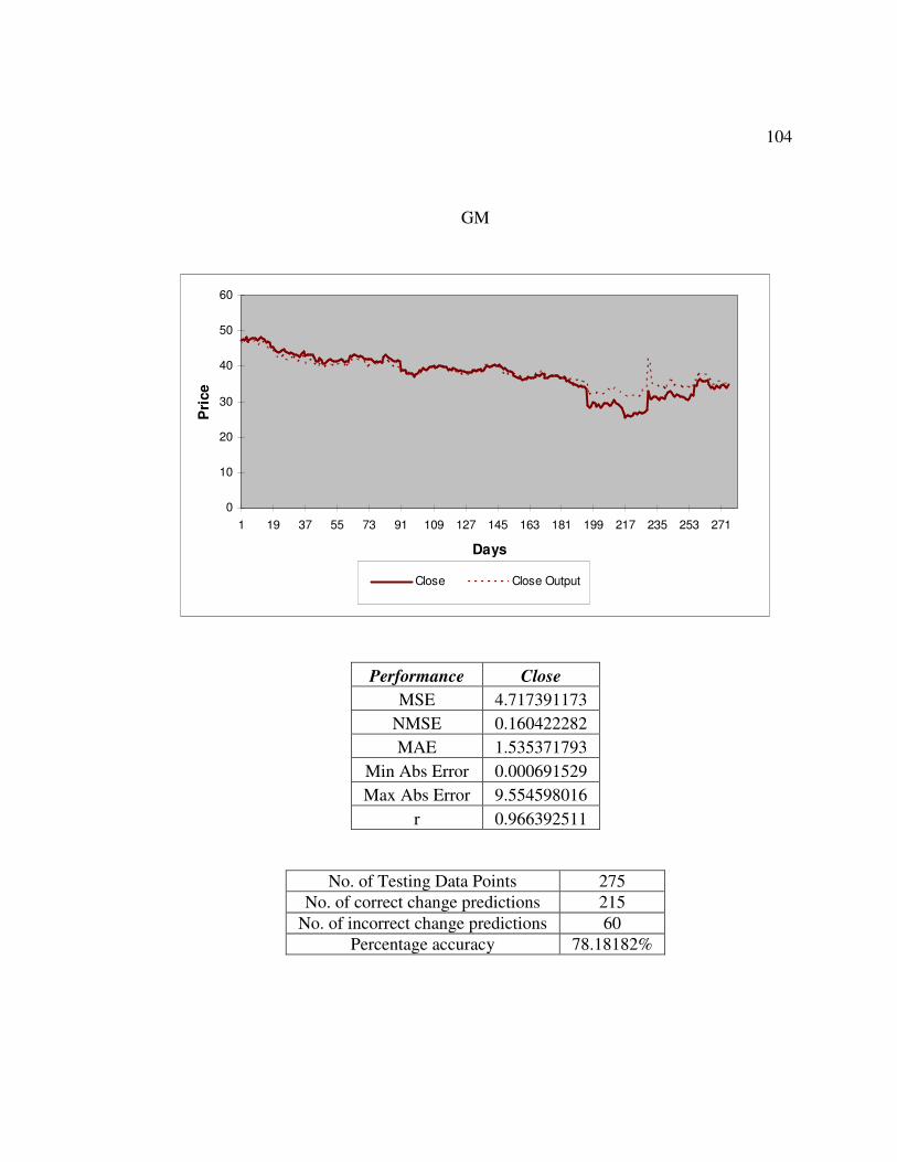
104

GM

0

10

20

30

40

50

60

1 19 37 55 73 91 109 127 145 163 181 199 217 235 253 271

Days

Pri

ce

Close Close Output


NMSE 0.160422282 MAE 1.535371793


r 0.966392511



105

HMC

0

5

10

15

20

25

30

1 19 37 55 73 91 109 127 145 163 181 199 217 235 253 271

Days

Pri

ce

Close Close Output


NMSE 3.918178502 MAE 1.813930673


R 0.947694484



106

HPQ

0

5

10

15

20

25

30

1 19 37 55 73 91 109 127 145 163 181 199 217 235 253 271

Days

Pri

ce

Close Close Output


NMSE 0.772060196 MAE 1.152977293


r 0.899925337



107

JPM

0

5

10

15

20

25

30

35

40

45

1 19 37 55 73 91 109 127 145 163 181 199 217 235 253 271

Days

Pri

ce

Close Close Output


NMSE 0.460987202 MAE 0.836601493


r 0.886060818



108

RHB

0

5

10

15

20

25

30

35

1 19 37 55 73 91 109 127 145 163 181 199 217 235 253 271

Days

Pri

ce

Close Close Output


NMSE 8.131775849 MAE 5.51226345


r 0.923858393



109

STX

0

5

10

15

20

25

1 19 37 55 73 91 109 127

Days

Pri

ce

Close Close Output


NMSE 0.172561269 MAE 0.40890251


r 0.925677312



110

WB

0

10

20

30

40

50

60

1 19 37 55 73 91 109 127

Days

Pri

ce

Close Close Output


NMSE 2.267040489 MAE 4.162225606


r 0.947567809



111

WLP

0

20

40

60

80

100

120

140

1 19 37 55 73 91 109 127

Days

Pri

ce

Close Close Output


NMSE 1.035705498 MAE 19.02542735


r 0.899617949



112

APPENDIX C

Final Model Results AGP

0

10

20

30

40

50

60

70

80

90

1 19 37 55 73 91 109 127 145

Days

Pri

ce

Close Close Output


NMSE 0.867207963 MAE 6.806080835


r 0.995744687



113

AMR

0

2

4

6

8

10

12

14

16

1 19 37 55 73 91 109 127 145 163 181 199 217 235 253 271

Days

Pri

ce

Close Close Output


NMSE 0.182064442 MAE 0.603707153


r 0.966350952



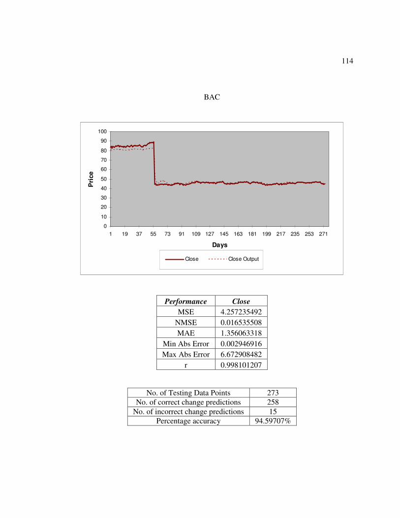
114

BAC

0

10

20

30

40

50

60

70

80

90

100

1 19 37 55 73 91 109 127 145 163 181 199 217 235 253 271

Days

Pri

ce

Close Close Output


NMSE 0.016535508 MAE 1.356063318


r 0.998101207



115

CAL

0

2

4

6

8

10

12

14

16

1 19 37 55 73 91 109 127 145 163 181 199 217 235 253 271

Days

Pri

ce

Close Close Output


NMSE 2.021538401 MAE 0.200968788


r 0.998818662



116

DAL

0

1

2

3

4

5

6

7

8

9

1 19 37 55 73 91 109 127 145 163 181 199 217 235 253 271

Days

Pri

ce

Close Close Output


NMSE 1.811855497 MAE 1.408527979


r 0.983171582



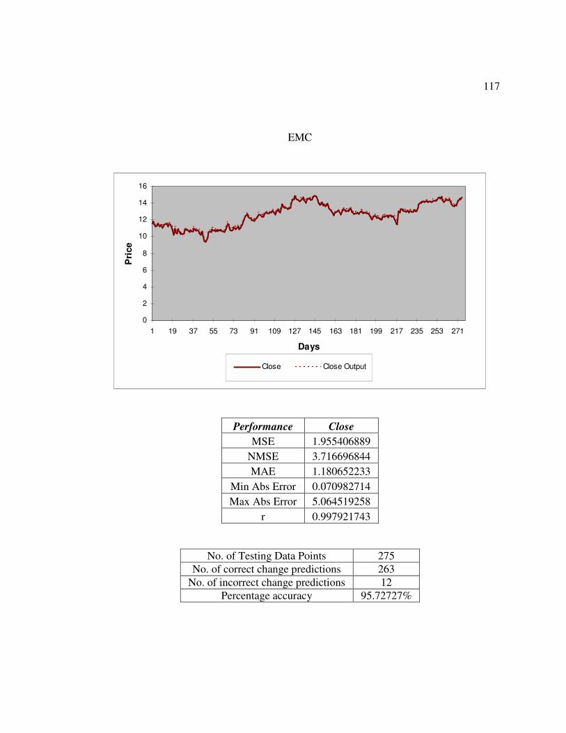
117

EMC

0

2

4

6

8

10

12

14

16

1 19 37 55 73 91 109 127 145 163 181 199 217 235 253 271

Days

Pri

ce

Close Close Output


NMSE 3.716696844 MAE 1.180652233


r 0.997921743



118

F

0

2

4

6

8

10

12

14

16

18

1 19 37 55 73 91 109 127 145 163 181 199 217 235 253 271

Days

Pri

ce

Close Close Output


NMSE 0.11271889 MAE 0.502675338


r 0.990866476



119

GM

0

10

20

30

40

50

60

1 19 37 55 73 91 109 127 145 163 181 199 217 235 253 271

Days

Pri

ce

Close Close Output


NMSE 0.127579883 MAE 1.459430414


r 0.961030293



120

HMC

0

5

10

15

20

25

30

1 19 37 55 73 91 109 127 145 163 181 199 217 235 253 271

Days

Pri

ce

Close Close Output


NMSE 0.631993112 MAE 0.292926656


r 0.997334054



121

HPQ

0

5

10

15

20

25

30

1 19 37 55 73 91 109 127 145 163 181 199 217 235 253 271

Days

Pri

ce

Close Close Output


NMSE 1.107359063 MAE 0.640282869


r 0.994390039



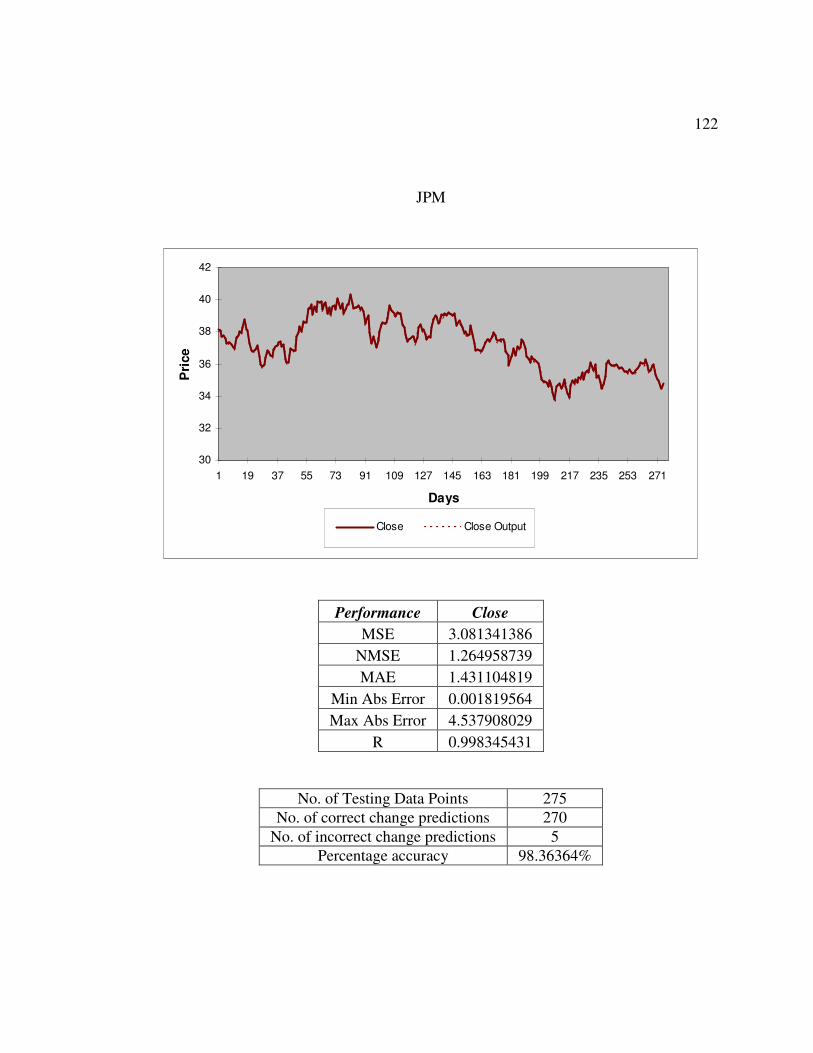
122

JPM

30

32

34

36

38

40

42

1 19 37 55 73 91 109 127 145 163 181 199 217 235 253 271

Days

Pri

ce

Close Close Output


NMSE 1.264958739 MAE 1.431104819


R 0.998345431



123

RHB

0

5

10

15

20

25

30

35

1 19 37 55 73 91 109 127 145 163 181 199 217 235 253 271

Days

Pri

ce

Close Close Output


NMSE 0.425815386 MAE 1.485770902


R 0.979754775



124

STX

0

5

10

15

20

25

1 19 37 55 73 91 109 127

Days

Pri

ce

Close Close Output


NMSE 0.162561708 MAE 0.418947599


R 0.95336365



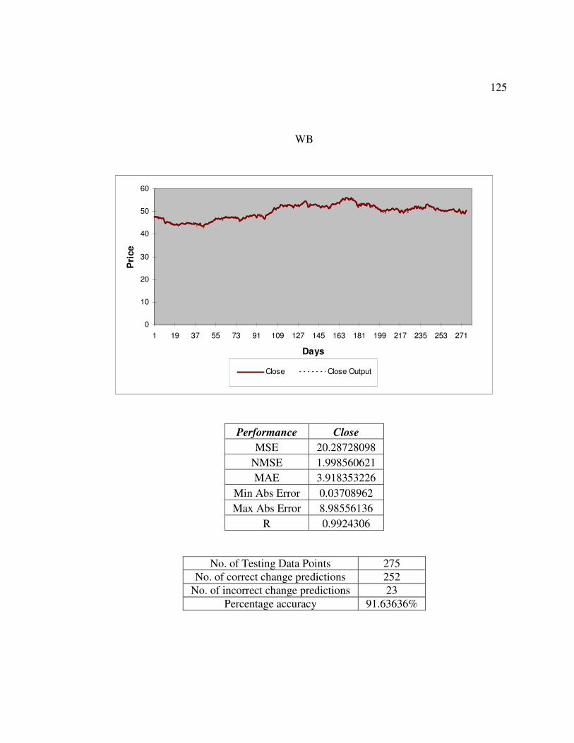
125

WB

0

10

20

30

40

50

60

1 19 37 55 73 91 109 127 145 163 181 199 217 235 253 271

Days

Pri

ce

Close Close Output


NMSE 1.998560621 MAE 3.918353226


R 0.9924306



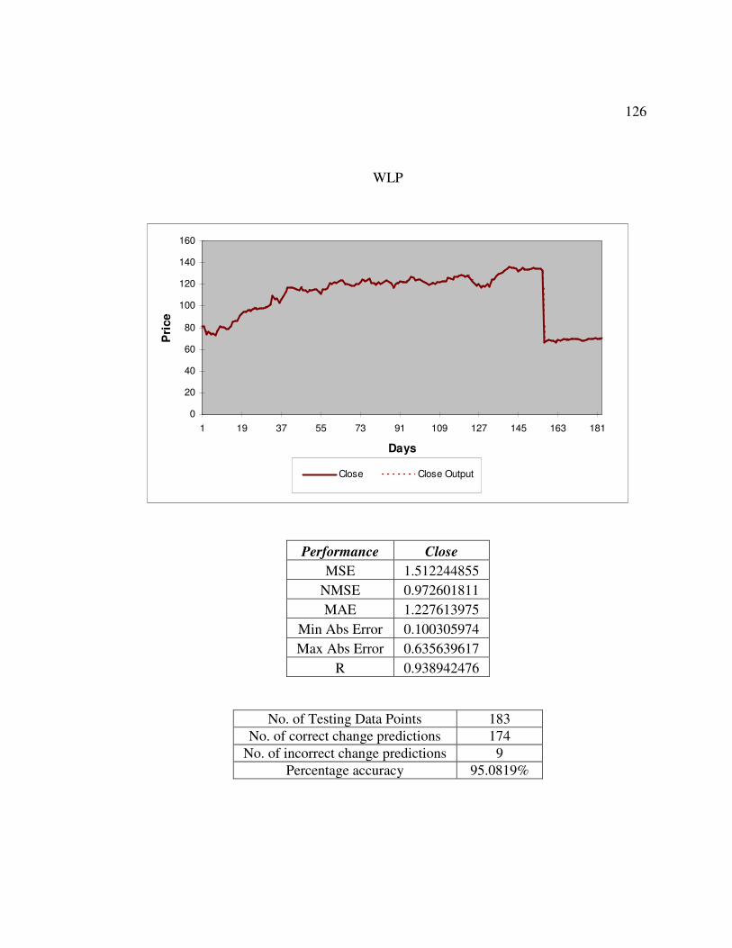
126

WLP

0

20

40

60

80

100

120

140

160

1 19 37 55 73 91 109 127 145 163 181

Days

Pri

ce

Close Close Output


NMSE 0.972601811 MAE 1.227613975


R 0.938942476



AN INTEGRATED STOCK MARKET FORECASTING MODEL USING

Documents

Transcript of AN INTEGRATED STOCK MARKET FORECASTING MODEL USING