Forecasting Stock Index Volatility:

The Incremental Information in the

Intraday High-Low Price Range

Charles Corrado Massey University - Albany

Auckland, New Zealand

Cameron Truong

University of Auckland Auckland, New Zealand

November 2004

Abstract

We compare the incremental information content of implied volatility and intraday high-low range volatility in the context of conditional volatility forecasts for three major market indexes: the S&P 100, the S&P 500, and the Nasdaq 100. Evidence obtained from out-of-sample volatility forecasts indicates that neither implied volatility nor intraday high-low range volatility subsumes entirely the incremental information contained in the other. Our findings suggest that intraday high-low range volatility can usefully augment conditional volatility forecasts for these market indexes.

JEL classification: C13, C22, C53, G13, G14 Keywords: options; implied volatility; volatility forecasting Please direct inquiries to: Charles Corrado, Department of Commerce, Massey University - Albany, Private Bag 102 904 NSMC, Auckland, New Zealand. c.j.corrado@massey.ac.nz; or, Cameron Truong, Department of Accounting & Finance, University of Auckland, Private Bag 92019, Auckland, New Zealand. c.truong@auckland.ac.nz

2

Forecasting Stock Index Volatility:

The Incremental Information in the

Intraday Price Range

Abstract

We compare the incremental information content of implied volatility and intraday high-low range volatility in the context of conditional volatility forecasts for three major market indexes: the S&P 100, the S&P 500, and the Nasdaq 100. Evidence obtained from out-of-sample volatility forecasts indicates that neither implied volatility nor intraday high-low range volatility subsumes entirely the incremental information contained in the other. Our findings suggest that intraday high-low range volatility can usefully augment conditional volatility forecasts for these market indexes.

I. Introduction

Since the development of autoregressive conditional heteroscedasticity (ARCH)

models by Engle (1982) and their generalization (GARCH) by Bollerslev (1986, 1987),

ARCH modeling has become the bedrock for dynamic volatility models. While originally

formulated to forecast conditional variances as a function of past variances, the inherent

flexibility of ARCH modeling allows ready inclusion of other volatility measures as well.

Consequently, extensive research has focused on evaluating other volatility measures that

might improve conditional volatility forecasts. One popular volatility measure used to

augment ARCH forecasts is implied volatility from option prices. Lamoureux and

Lastrapes (1993) find that an ARCH model provides superior volatility forecasts than

implied volatility alone in a sample of 10 stock return series. However, Day and Lewis

(1992) report that a mixture of implied volatility and ARCH forecasts of future return

volatility for the S&P 100 stock index outperforms separate forecasts from implied

volatility or ARCH alone. More recently, Mayhew and Stivers (2003) find that implied

volatility improves GARCH volatility forecasts for individual stocks with high options

trading volume. They report that for stocks with the most actively traded options, implied

volatility reliably outperforms GARCH and subsumes all information in return shocks

beyond the first lag.

3

Another volatility measure that has become popular with the increasing

availability of intraday security price data is an intraday variance computed by summing

the squares of intraday returns sampled at short intraday intervals. Essentially, if the

security price path is continuous then increasing the sampling frequency yields an

arbitrarily precise estimate of return volatility (Merton, 1980). The efficacy of intraday

return variances has been demonstrated with foreign exchange data by Andersen et al.

(2001b), Andersen, Bollerslev, and Lange (1999), Andersen and Bollerslev (1998), and

Martens (2001) and with stock market data by Andersen et al. (2001a), Areal and Taylor

(2002), Fleming, Kirby, and Ostdiek (2003), and Martens (2002). Indeed as a competitor

to implied volatility, Taylor and Xu (1997), Pong, Shackleton, Taylor, and Xu (2003),

and Neely (2002) report that intraday return variances from the foreign exchange market

provide incremental information content beyond that provided by implied volatility

forecasts. By contrast, Blair, Poon, and Taylor (2001) find that the incremental

information content of intraday return variances for the S&P 100 stock index is scant and

that an implied volatility index published by the Chicago Board Options Exchange

(CBOE) provides the most accurate forecasts at all forecast horizons.

We extend the volatility forecasting literature cited above with the specific

objective of demonstrating the usefulness of the intraday high-low price range for

improving volatility forecasts for three major stock market indexes: the S&P 100, the

S&P 500, and the Nasdaq 100. This study represents the first attempt to compare the

effectiveness of the intraday high-low price range and implied volatility as forecasts of

future realized volatility for these market indexes.

We find that the intraday high-low range volatility estimator provides incremental

information content beyond that already contained in implied volatility indexes published

by the Chicago Board Options Exchange (CBOE). This is demonstrated by comparing

augmented volatility forecasts based around the asymmetric GARCH model developed

by Glosten et al. (1993) and Zakoian (1990), hereafter referred to as GJR-GARCH. Our

findings suggest that intraday high-low range volatility can usefully augment conditional

volatility forecasts for the three broad market indexes examined.

4

There are several reasons to consider the intraday high-low price range for

volatility measurement and forecasting. Firstly, high-low price range data has long been

available in the financial press and is often available when high-frequency intraday

returns data are not. Secondly, Andersen and Bollerslev (1998) point out that market

microstructure issues such as nonsynchronous trading effects, discrete price observations,

and bid-ask spreads, etc. may limit the effectiveness of intraday return variances as

volatility forecasts. For example, Andersen et al. (1999) report that sampling intraday

returns at one-hour intervals provided better results than sampling at 5-minute intervals in

their study of foreign exchange market volatility. The intraday high-low price range may

offer a useful alternative to an intraday return variance when market microstructure

effects are severe. Indeed, Alizadeh et al. (2002) suggest that, “Despite the fact that the

range is a less efficient volatility proxy than realized volatility under ideal conditions, it

may nevertheless prove superior in real-world situations in which market microstructure

biases contaminate high-frequency prices and returns.”

Thirdly, in addition to potential market microstructure biases Bai, Russell, and

Tiao (2001) point out that the estimation efficiency of an intraday return variance

estimator can be sensitive to non-normality in intraday returns data. As a basic

demonstration of potential sensitivity to non-normality, let rd and rh denote a one-day

return and an intraday return, respectively, such that the one-day return is the sum of

n intraday returns, i.e., 1

n

d hh

r r=

= ∑ . Assuming that the n intraday returns are identically,

independently distributed (iid), with an expected value of zero, i.e., ( ) 0hE r = , then the

sum of the squared intraday returns is an unbiased estimator of the daily return variance.

( )2

1 1

n n

h h dh h

E r Var r Var r= =

= = ∑ ∑ (1)

Theoretically, the efficiency of the squared intraday returns volatility estimator specified

in equation (1) increases monotonically by dividing the trading day into finer increments.

A general statement of this proposition is provided by the following theorem:

5

Theorem

The variance of the squared intraday returns volatility estimator, i.e., 2

1

n

hh

Var r=

∑ ,

assuming iid squared intraday returns with zero expected value is given by the expression

immediately below, in which Kurt(rd) and Kurt(rh) denote the kurtosis of daily

returns and intraday returns, respectively.

( )

( ) ( )( )( )( )( ) ( )( )

( )( ) ( )( )

( )( ) ( )

2 2

1 1

24

12

2

2

1

1

23

n n

h hh h

n

h hh

h h

hd

d d

Var r Var r

E r Var r

n Var r Kurt r

Kurt rVar r

n

Var r Kurt rn

= =

=

=

= −

= × −

−= ×

= × − +

∑ ∑

∑

(2)

The last equality on the right-hand side of equation (2) above is an immediate

consequence of the assumption of iid intraday returns, for which the following

relationship holds as an adjunct to the Central Limit Theorem:1

( ) ( )( )3 3h dKurt r n Kurt r− = × − (3)

Thus, with given values for the variance and kurtosis of daily returns, i.e., Var(rd)

and Kurt(rd), the variance of the squared intraday returns volatility estimator declines

monotonically as n increases.

However as shown in the last line of equation (2), the variance of the squared

intraday returns volatility estimator is bounded away from zero for non-normally

distributed returns with Kurt(rd) > 3. The theoretical relative efficiency of the squared

intraday returns volatility estimator to the squared daily return volatility estimator as a

function of return kurtosis is stated in equation (4) immediately below.

( ) ( )( )

2

2

1

123

d dn

dhh

Var r Kurt r

Kurt rVar r n=

−=

− + ∑

(4)

1 An appendix provides a derivation.

6

With exactly normally distributed returns, i.e., Kurt(rd) = 3, this relative efficiency

is bounded only by the number of intraday return intervals n. However for plausible

kurtosis values, the relative efficiency in equation (4) can be severely bounded. For

example, a daily return kurtosis of Kurt(rd) = 4 with n = 79 intraday return intervals

yields a theoretical relative efficiency of just 2.93.2

Parkinson (1980) shows that the intraday high-low price range volatility estimator

has a theoretical relative efficiency of 4.762 compared to a squared daily return.

However, this value assumes normally distributed returns. To assess relative efficiency

with non-normally distributed returns, we use Monte Carlo simulation experiments with

various return kurtosis values. We then simulate intraday returns over n = 79 intraday

intervals for each of 100,000 trading days. Kurtotic intraday returns are generated by

random sampling from a mixture of normals, where with probability p a random normal

variate is drawn with variance 2pσ and with probability 1-p is drawn with variance 2

1 pσ − .

The probability p and the ratio of variances determine the kurtosis of the normals

mixture:

( )( )

4 41

22 21

3 / 1

/ 1p p

p p

p pKurtosis

p p

σ σ

σ σ

−

−

+ −=

+ −

Following a convenient specification, we set p = 1/Kurtosis to solve for 2σ as,

( )( )2

21 3 2 1

2

Kurtosis Kurtosisσ

− + − −= .

In each simulated trading day, we compute the sum of squared intraday returns, the

squared daily return, and the squared high-low range. Relative efficiencies computed

from these daily statistics averaged over 100,000 days are reported in the panel

immediately below.

2 Bai, Russell, and Tiao (2001) provide an extensive analysis of efficiency losses due to kurtosis and other effects with non-iid intraday returns.

7

Relative efficiencies of intraday variance estimators to squared daily return estimator with varied kurtosis.

Daily return

kurtosis

Squared intraday returns estimator

Squared intraday high-low range

estimator

Ratio

3.5 4.786 2.960 1.617 4.0 2.944 2.632 1.118 4.5 2.289 2.462 0.930 5.0 1.997 2.385 0.837

Comparing relative efficiencies for the squared intraday returns estimator and the squared

intraday high-low range estimator as shown in the panel above, we see that for plausible

kurtosis values the squared intraday returns volatility estimator may not be greatly more

efficient than the squared high-low range estimator. Indeed, for daily kurtosis values

higher than about 4.3 the squared high-low range estimator is more efficient than the

squared intraday returns estimator. Further, Alizadeh et al. (2002) suggest that the

intraday high-low range is robust to microstructure noise, while the squared intraday

returns estimator can be quite sensitive to such noise.

II. Data sources

This study is based on returns for the S&P 100, S&P 500, and Nasdaq 100 stock

market indexes, along with daily implied volatilities for these indexes published by the

Chicago Board Options Exchange (CBOE). Ticker symbols for the implied volatility

indexes are VIX for the S&P 500, VXO for the S&P 100, and VXN for the Nasdaq 100.3

Our data set spans the period January 1990 through December 2003 for the S&P 100 and

S&P 500 stock indexes, and from January 1995 through December 2003 for the

Nasdaq 100 stock index.

3 The CBOE previously used the ticker VIX for S&P 100 implied volatility, but began using VXO for S&P 100 implied volatility and VIX for S&P 500 implied volatility with the introduction of the latter series.

8

II.1. Daily index returns

Daily index returns are calculated as the natural logarithm of the ratio of

consecutive daily closing index levels.

( )1lnt t tr c c −= (5)

In equation (5), rt denotes the index return for day t based on index levels at the close of

trading on days t and day t-1, i.e., ct and ct-1, respectively.

II.2. Daily high-low price range

“..intuition tells us that high and low prices contain more information regarding to

volatility than do the opening and closing prices.” (Garman and Klass, 1980) For

example, by only looking at opening and closing prices we may wrongly conclude that

volatility on a given day is small if the closing price is near the opening price despite

large intraday price fluctuations. Intraday high and low values may bring more integrity

into an estimate of actual volatility.

In this study, we use the intraday high-low volatility measure specified in

equation (6), in which hit and lot denote the highest and lowest index levels observed

during trading on day t.

( )22 ln ln

4 ln 2t t

t

hi loRNG

−= (6)

This intraday high-low price range was originally suggested by Parkinson (1980) as a

measure of security return volatility.4

II.3 CBOE implied volatility indexes

Implied volatilities have long been used by academics and practitioners alike to

provide forecasts of future return volatility. In addition to studies cited earlier,

Christensen and Prabhala (1998) overcome the methodological difficulties in Canina and

Figlewski (1993) and show that by using non-overlapping data and an instrumental

variables econometric methodology that implied volatility outperforms historical

4 Interesting extensions to Parkinson (1980) have been developed by Garman and Klass (1980), Ball and Torous (1984), Rogers and Satchell (1991), Kumitomo (1992), and Yang and Zhang (2000).

9

volatility as a forecast of future return volatility for the S&P 100 index. Corrado and

Miller (2004) update and extend the Christensen and Prabhala study and suggest that

implied volatility continued to provide a superior forecast of future return volatility

during the period 1995 through 2003.

In this study, we use data for three implied volatility indexes published by the

Chicago Board Options Exchange (CBOE). These implied volatility indexes are

computed from option prices for options traded on the S&P 100, the S&P 500, and the

Nasdaq 100 stock indexes.

The implied volatility indexes with ticker symbols VIX and VXN are based on

European-style options on the S&P 500 and Nasdaq 100 indexes, respectively. These

indexes are calculated using the formula stated immediately below, in which C(K,T) and

P(K,T) denote prices for call and put options with strike price K and time to maturity T

stated in trading days. This formula assumes the option chain has strike prices ordered

such that 1j jK K+ > . The two nearest maturities are chosen with the restriction that

2 122 8T T≥ ≥ ≥ .

( ) ( )( ) ( ) ( )( )

21 1

21 12 1

221 min , , ,

Nh j jh

j h j hh j j

K KTVIX C K T P K T

T T K+ −

= =

−−= −

−∑ ∑ (7)

Theoretical justification for this calculation method is provided by Britten-Jones and

Neuberger (2000).

The implied volatility index with ticker symbol VXO is based on American-style

options on the S&P 100 index.5 This index is calculated using the formula stated

immediately below in which IVC(K,T) and IVP(K,T) are implied volatilities for call and

put options, respectively, with strike K and maturity T. The at-the-money strike Km

denotes the largest exercise price less or equal to the current cash index S0. Hence, the

volatility index VXO is calculated using only option contracts with strike prices that

bracket the current cash index level.

( ) ( )( ) ( ) ( )( )

( )( )

1 2

0 10 1

2 1 1

1 22 , ,j hh m j C m j h P m j h

j h

m m

T S K IV K T IV K TVXO

T T K K

++ − + +

= =

+

− − − +=

− −

∑∑ (8)

5 Authoritative descriptions of this implied volatility index are Whaley (1993) and Fleming, Ostdiek, and Whaley (1995).

10

To be scaled consistently with the other daily volatility measures, the implied

volatility indexes VXO, VIX, and VXN are all squared and divided by 252, the assumed

number of trading days in a calendar year.

[TABLE 1 HERE]

II.4 Descriptive statistics

Table 1 provides a statistical summary of the volatility data used in this study.

Panel A reports the mean, maximum, minimum, standard deviation, and skewness and

kurtosis coefficients for squared daily returns, squared implied volatilities, and squared

high-low price ranges for the S&P 100 index. Panels B and C report descriptive statistics

for the S&P 500 and Nasdaq 100 indexes, respectively.

The period January 1990 through December 2003 yields 3,544 daily observations

for the S&P 100 and S&P 500 indexes and the period January 1995 through December

2003 yields 2,266 daily observations for the Nasdaq 100 index. Table 1 reveals noticeable

statistical differences among the three volatility measures. For example, in all panels of

Table 1 the average squared high-low range volatility is smaller than the average squared

daily return, which in turn is smaller than the average squared implied volatility.

Comparing volatility measures across S&P 100, S&P 500, and Nasdaq 100 indexes it is

evident that volatility for the Nasdaq 100 is highest among the three indexes. Indeed, the

average squared daily return for the Nasdaq 100 index is on average four to five times

larger in magnitude than average squared daily returns for the S&P 100 and S&P 500

indexes.

III. Forecast methodology

To model market volatility dynamics we draw on the GJR-GARCH model

specification developed by Glosten et al. (1993) and Zakoian (1990). This model attempts

to capture the asymmetric effects of good news and bad news on conditional volatility.

We augment the basic GJR-GARCH model with implied volatility and intraday high-low

price range volatility.

11

III.1 Augmented GJR-GARCH model

Augmented by implied volatility and the intraday high-low range, the GJR-

GARCH model for conditional variance is specified in equation (9) immediately below,

in which the dummy variable 1−ts = 1 if 1−tε < 0 and is zero otherwise.

2 2 2 20 1 1 2 1 1 1 1 1

t t

t t t t t t t

r

h s h IVOL RNG

µ ε

α α ε α ε β γ δ− − − − − −

= +

= + + + + + (9)

rt return on day t

ht conditional volatility on day t

IVOLt implied volatility at end of index options trading on day t

RNGt intraday high-low range volatility on day t

In this model, good news ( 1−tε > 0), and bad news ( 1−tε < 0) have differential impacts on

conditional variance. The impact of good news alone is measured by the coefficient 1α ,

while the impact of bad news is measured by the sum of coefficients 21 αα + . A priori we

expect 2α alone as well as the sum 21 αα + to be positive. Lagged implied volatility and

lagged high-low range volatility measures become additional explanatory variables to

augment the basic GJR-GARCH model.

By placing varied restrictions on parameters, we obtain four different volatility

models that compare the incremental forecast information of implied volatility and high-

low price range volatility. These four models are specified immediately below.

1) GJR-GARCH(1,1) model: The GJR-GARCH(1,1) model is implemented by setting the

restrictions 0== δγ . This specification yields a model with no exogenous regressors. 2 2

0 1 1 2 1 1 1t t t t th s hα α ε α ε β− − − −= + + + (10)

2) High-low range volatility excluded: This specification has the single restriction 0=δ

to exclude intraday high-low range volatility. It combines the GJR-GARCH(1,1) model

with lagged implied volatility as an additional regressor to assess the incremental

information content of implied volatility. 2 2 2

0 1 1 2 1 1 1 1t t t t t th s h IVOLα α ε α ε β γ− − − − −= + + + + (11)

12

3) Implied volatility excluded: This specification has the single restriction 0=γ to

exclude implied volatility. It combines the GJR(1,1) model with intraday high-low range

volatility. Comparison with the basic GJR(1,1) model yields an assessment of the

incremental information content of the high-low price range volatility. 2 2 2

0 1 1 2 1 1 1 1t t t t t th s h RNGα α ε α ε β δ− − − − −= + + + + (12)

4) Unrestricted model: This specification has no restrictions and therefore represents a

complete implementation of equation (9), which is reproduced here for convenient

reference. 2 2 2 2

0 1 1 2 1 1 1 1 1t t t t t t th s h IVOL RNGα α ε α ε β γ δ− − − − − −= + + + + +

Parameter estimates for all four specifications stated above are obtained by a

quasi-likelihood methodology, by which covariances and standard errors are computed

using methods suggested in Bollerslev and Wooldridge (1992).

III.2 Large-sample adjustments to critical t-values

Connolly (1989) points out that the large sample sizes characteristic of many

financial studies can lead to an overstatement of statistical significance due to Lindley’s

paradox (Lindley, 1957). To alleviate this potential bias, Leamer (1978) suggests that

critical values for regression test statistics be adjusted to reduce the likelihood of Type II

errors. In equation (13) below presents the adjustment for t-statistics of regression

coefficients, where T is the sample size and k is the number of degrees of freedom lost in

the regression.

( )* 1/ 1Tt T k T= − × − (13)

When the absolute value of a calculated t-statistic is greater than the value computed by

equation (13), the absolute value of the calculated t-statistic is reduced by the adjustment

in equation (13). We follow this procedure whenever the sample size exceeds 200.

13

III.3 Out-of-sample forecasts

Each of the four GJR-GARCH models specified above provides out-of-sample

volatility forecasts over N = 1, 10, 20 days. We begin by calibrating each model using

parameters estimated over an initial estimation period. For S&P 100 and S&P 500

indexes, we use the first 2,000 days of data as an initial parameter estimation period. Due

to a shorter time span of available Nasdaq 100 data, we use only the first 1,000 days of

data as an initial parameter estimation period. After the initial parameter estimation, each

GJR-GARCH model yields out-of-sample volatility forecasts over the N = 1, 10, 20 days

immediately subsequent to the estimation period. One-day forecasts are obtained directly

from each model specification, while N = 10, 20-day forecasts are generated by

multiplying the one-day volatility forecast by N. Along with these N = 1, 10, 20-day

volatility forecasts, corresponding realized volatilities from the N = 1, 10, 20-day forecast

periods are computed as the sum of squared daily returns in the N-day forecast period.

After initial parameter estimation and forecast construction, the entire procedure

is repeated by rolling forward the parameter estimation period and re-estimating GJR-

GARCH model parameters. This procedure is repeated through all remaining data. For

the S&P 100 and S&P 100 indexes, this ultimately yields 1,541 one-day forecasts, 154

10-day forecasts, and 77 20-day volatility forecasts. For the Nasdaq 100 index, this yields

1,266 one-day forecasts, 126 10-day forecasts, and 63 20-day volatility forecasts. All

volatility forecasts are non-overlapping, out-of-sample forecasts.

Figure I provides a graphical illustration of out-of-sample one-day volatility

forecasts. Panel A and Panel B display daily realized and forecast volatility values for the

1,541 one-day forecasts for the S&P 100 and S&P 500 stock indexes, respectively.

Panel C displays daily realized and forecast volatility values for the 1,266 one-day

forecasts for the Nasdaq 100 index. While Figure I suggests that the volatility forecasts

capture a large proportion of the variability of predictable volatility, a formal evaluation

of forecast efficacy is provided immediately below.

[FIGURE I]

14

III.4 Forecast efficiency evaluations

To evaluate the accuracy of the out-of-sample volatility forecasts Blair et al.

(2001) suggest the P-statistic specified in equation (13), which measures the proportion

of the variance of realized volatilities explained by volatility forecasts. In this P-statistic,

,t Ny and ,t Ny denote realized and forecast volatility values over a N-day forecast horizon

beginning on day t.

( )( )

( )( )

/2

( 1), ( 1),1

/2

( 1),1

1

T S N

S N i n S N i Ni

T S N

S N i Ni

y yP

y y

−

+ × − + × −=

−

+ × −=

−= −

−

∑

∑ (14)

For the data used in is study the parameters of equation (14) are T = 3,544 and S = 2,001

for the S&P 100 and S&P 500 indexes, T = 2,266 and S = 1,001 for the Nasdaq 100

index, and N = 1, 10, 20 for the three different forecast horizons.

Two additional measures of forecast accuracy are the Root Mean Squared Error

(RMSE) and Mean Absolute Error (MAE); these are computed as shown in equations (15)

and (16) immediately below.

( ) ( ) ( )( )( ) / 2

1 , 1 ,1

1/

T S N

S N i N S N i Ni

RMSE y yT S N

−

+ × − + × −=

= −− ∑ (15)

( ) ( ) ( )

( ) /

1 , 1 ,1

1/

T S N

S N i N S N i Ni

MAE y yT S N

−

+ × − + × −=

= −− ∑ (16)

An alternative measure of forecast ability is the R-squared from the regression of

an N-day realized volatility ,t Ny on the corresponding forecast volatility ,t Ny , as

specified in equation (17).

, ,t N t N ty y eα β= + + (17)

To simultaneously compare forecasts made from Model 2 and Model 3, we

regress realized volatility on forecasts from Model 2 and Model 3 as specified in

equation (18), in which 2,Mt Ny denotes an N-day forecast from Model 2 and 3

,Mt Ny denotes

an N-day forecast from Model 3. 2 3

, 1 2 , 3 ,ˆ ˆM Mt N t N t N ty a a y a y e= + × + × + (18)

15

The R-squared of this regression is a measure of information content based on the

proportion of volatility variance explained by the best linear function of the forecasts.

[INSERT TABLE 2]

IV. Empirical results

IV.1 Full sample GJR-GARCH model results

Table 2 presents GJR-GARCH parameter estimates and related statistics obtained

from all available data for the three stock indexes. In Table 3, Panel A reports results

obtained from S&P 100 index data, Panel B corresponds to S&P 500 index data, and

Panel C reports results from Nasdaq 100 data. Parameter estimates are reported in

columns 2 through 7, with robust t-statistics reported in parentheses below each

coefficient estimate. Log-likelihood values are listed in column 8, with Durbin-Watson

statistics listed in column 9. All Durbin-Watson statistics indicate an absence of

significant autocorrelations in regression errors.

Panels A and B of Table 2 corresponding to S&P 100 and S&P 500 indexes,

respectively, show that log-likelihood statistics in column 8 increase monotonically

moving from Model 1 to Model 4. For the Nasdaq 100, Panel C reveals a similar pattern,

except that the log-likelihood value for Model 2 greater than that for Model 3.

For all models and indexes, the GJR-GARCH coefficients 1α measuring the

impact of good news are never significantly positive and in some cases are significantly

negative. By contrast, the coefficients 2α are always significantly positive and the

coefficient sums 1 2α α+ are always positive. Thus, overall we observe a pervasive

asymmetric effect of past daily returns on conditional volatility in which bad news

( 1−tε < 0) has a strong impact on conditional variance while good news ( 1−tε > 0) has a

much weaker effect. This is consistent with empirical findings in Blair et al. (2001) who

also find that past volatility has a similar asymmetric impact on conditional volatility.

The augmented GJR-GARCH specification for Model 2 excludes only intraday

high-low range volatility and that for Model 3 excludes only implied volatility. In all

three panels of Table 2, Model 2 yields significant regression coefficients for implied

16

volatility and Model 3 yields significant regression coefficients for high-low range

volatility. For the S&P 100 and S&P 500 indexes, Panels A and B reveal that log-

likelihood values for Model 3 are smaller than those for Model 2, thereby suggesting that

high-low range volatility has greater information content than does implied volatility.

However for the Nasdaq 100 index, Panel C reveals that the log-likelihood value for

Model 2 is smaller than that of Model 3, suggesting that implied volatility has greater

information content than intraday high-low range volatility for that index.

Notwithstanding these differences, the results obtained from Model 4 for all three indexes

indicate significant slope coefficients for both intraday high-low range volatility and

implied volatility. This suggests that both volatility measures provide incremental

information content not entirely subsumed by the other.

[TABLE 3]

IV.2 Out-of-sample forecast evaluation

Table 3 summarizes out-of-sample accuracy of volatility forecasts from various

GJR-GARCH model specifications by reporting P-statistics, root mean squared errors

(RMSE), and mean absolute errors (MAE) of volatility forecasts for the S&P 100,

S&P 500, and Nasdaq 100 indexes. Results for N = 1, 10, 20 day-forecasts are reported.

Perhaps the most notable aspect of the out-of-sample volatility forecast results

reported in Table 3 is the contrasting performance between Model 1 and Model 4.

Model 1 represents the basic GJR-GARCH model, while Model 4 is the GJR-GARCH

model augmented by both intraday high-low range volatility and implied volatility.

Model 4 displays markedly improved performance over Model 1 across all three stock

indexes and all forecast horizons. For example, one-day volatility forecasts for the

S&P 100, S&P 500, and Nasdaq 100 indexes from Model 1 yield P-statistic values of

0.117, 0.121, and 0.141, respectively. By contrast, Model 4 yields P-statistic values of

0.147, 0.145, and 0.172 for corresponding one-day forecasts. Similarly for 20-day

volatility forecasts, Model 1 yields P-statistic values of 0.243, 0.294, and 0.407, while

Model 4 yields corresponding values of 0.367, 0.425, and 0.534. These results clearly

indicate that volatility forecasts formed from the GJR-GARCH model are appreciably

17

improved with the additional information contained in implied volatility and high-low

range volatility for all three stock indexes at all forecast horizons. Essentially the same

results are reflected in the RMSE and MAE statistics.

Looking more closely at Table 3, a specific comparison of results obtained from

Model 2 and Model 3 holds some interest. Model 2 excludes only high-low range

volatility and Model 3 excludes only implied volatility. P-statistics in Panel A of Table 4

shows that Model 3 yields superior volatility forecasts to Model 2 at all forecast horizons

for the S&P 100 index. By contrast, Model 2 yields P-statistics indicating superior

forecasts to Model 3 for Nasdaq 100 volatility forecasts at all forecast horizons. Results

are mixed for the S&P 500 index, for which Model 3 yields P-statistics indicating a

superior volatility forecast to Model 2 at the one-day horizon, an inferior forecast at the

10-day horizon, and nearly equivalent forecast performance at the 20-day horizon. Thus

the evidence presented here does not indicate uniformly superior forecast performance for

either the high-low range volatility or implied volatility alone. However, both Model 2

and Model 3 provide uniformly superior forecast performance over Model 1 indicating

that both intraday high-low range volatility and implied volatility contain information not

captured by Model 1.

[TABLE 4]

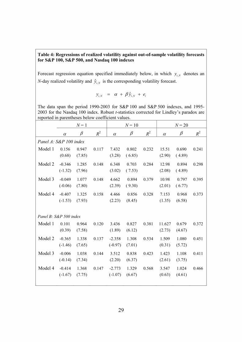
Table 4 reports R-squared values and coefficient values from regressions of

realized volatility on out-of-sample volatility forecasts across the four models, three

indexes, and three forecast horizons. Panel A reports results from S&P 100 volatility

forecasts, Panel B reports results for S&P 500 volatility forecasts, and Panel C reports

results for Nasdaq 100 volatility forecasts.

The R-squared values shown in Panel A of Table 4 indicate that Model 3 yields

out-of-sample S&P 100 volatility forecasts superior to those obtained from Model 2 at

forecast horizons of 10 and 20 days. However, for one-day S&P 100 volatility forecasts

the R-squared value of 0.148 is the same for both Model 3 and Model 2. Since Model 3

excludes only implied volatility and Model 2 excludes only intraday high-low range

volatility, at the one-day horizon both implied volatility and intraday high-low range

18

volatility for the S&P 100 index appear to provide similar information content. However,

at the 10-day and 20-day horizons it appears that much of the incremental information

contained in implied volatility is subsumed by intraday high-low range volatility. The

relative weakness of implied volatility at 10-day and 20-day horizons is surprising since

the VXO volatility index represents a volatility forecast over a 22-day horizon.

Panel B of Table 4 reveals that Model 3 yields out-of-sample S&P 500 volatility

forecasts superior to those obtained from Model 2 at the one-day forecast horizon, with

R-squared values of 0.144 and 0.137, respectively. However, Model 3 yields volatility

forecasts inferior to Model 2 at the 10-day horizon, with R-squared values of 0.423 and

0.534, respectively. Similarly, Model 3 and Model 2 yield R-squared values of 0.411 and

0.451, respectively, at the 20-day forecast horizon. In this case, the relative strength of

implied volatility at the 10-day and 20-day forecast horizons is expected since the VIX

volatility index is constructed to represent a 22-day volatility forecast.

In contrast to results reported from Panel A, R-squared values shown in Panel C

of Table 4 indicate that Model 2 provides superior Nasdaq 100 volatility forecasts at all

forecast horizons compared to those obtained from Model 3. For one-day Nasdaq 100

volatility forecasts, the R-squared value of 0.183 for Model 2 is almost identical to the

value of 0.186 for Model 4, while that for Model 3 is 0.159. Thus, at the one-day horizon

it appears that the incremental information contained in intraday high-low range volatility

is largely subsumed by implied volatility. At the 10-day forecast horizon, the R-squared

values for Model 2 and Model 4 are both 0.592, while the corresponding value for

Model 3 is 0.456. Similarly at the 20-day forecast horizon, Model 2 and Model 4 yield

the same R-squared value of 0.395, while Model 3 yields an R-squared value of 0.350.

Thus, at all volatility forecast horizons for the Nasdaq 100 index the incremental

information contained in intraday high-low range volatility appears to be already

subsumed by implied volatility.

Overall, the results shown in Table 4 mirror and reinforce those shown in Table 3.

These all indicate that intraday high-low range volatility contains incremental

information beyond that contained in implied volatility for out-of-sample S&P 100

volatility forecasts at all forecast horizons. However, implied volatility provides

incremental information beyond that contained in intraday high-low range volatility for

19

Nasdaq 100 volatility forecasts at all forecast horizons. For out-of-sample S&P 500

volatility forecasts, the results are mixed. The intraday high-low range appears to provide

some incremental information over implied volatility at one-day and 20-day horizons, but

results favor implied volatility at a 10-day horizon.

In all cases examined, both intraday high-low range volatility and implied

volatility bring significant improvements to the GJR-GARCH model. Model 2 and

Model 3 clearly outperform Model 1 with all indexes across all forecast horizons. Thus,

intraday high-low range volatility and implied volatility both provide incremental

information for forecasting conditional volatility.

[TABLE 5]

To assess the relative contributions of high-low range volatility and implied

volatility to improved conditional volatility forecasts, Table 5 reports results from

regressions of realized volatility against competing out-of-sample forecasts. In these

regressions, the coefficients 2α and 3α represent slope coefficients for forecasts from

Model 2 and Model 3, respectively. In general, slope coefficients for both Model 2

forecasts and Model 3 forecasts are significant across all indexes and forecast horizons.

Two exceptions occur for Nasdaq 100 regressions with one-day and 20-day forecast

horizons for which the coefficient 3α has t-statistic values of just 0.76 and 0.19,

respectively. An exception also occurs for S&P 500 regressions where the coefficient 3α

for the 20-day forecast horizon is just 1.56.

The results reported in Table 5 further support those reported in Table 3 and

Table 4. The coefficient 3α for Model 2 forecasts is uniformly larger than the coefficient

2α for Model 3 forecasts at all forecast horizons for the S&P 100 index, indicating

relatively greater information content for intraday high-low range volatility. However, the

coefficient 2α is uniformly larger than the coefficient 3α at all forecast horizons for the

S&P 500 index and the Nasdaq 100 index, indicating relatively greater information

content for implied volatility.

20

V. Summary and conclusions

This is the first study to compare the incremental information content of the

intraday high-low price range and implied volatility when used to augment GARCH

model forecasts of stock market volatility. We examine conditional volatility forecasts for

three broad market indexes: the S&P 100 and the S&P 500 over the period January 1990

through December 2003, and the Nasdaq 100 over the period January 1995 through

December 2003. Our results strongly support the conclusion that volatility forecasts

formed from a GJR-GARCH model are appreciably improved with the additional

information contained in implied volatility and high-low range volatility.

We also find that the intraday high-low range often provides significant

incremental information beyond that already contained in a GARCH model augmented

by implied volatility. This is demonstrated by comparing conditional volatility forecasts

based on various configurations of the GJR-GARCH model augmented by implied

volatility and intraday high-low range volatility.

For the S&P 100 index volatility forecasts, we find evidence supporting the

conclusion that intraday high-low range volatility provides greater incremental

information than implied volatility over one-day, 10-day, and 20-day forecast horizons.

However, results obtained from Nasdaq 100 index volatility forecasts indicate that

implied volatility provides greater information content than intraday high-low range

volatility over all volatility forecast horizons. For S&P 500 index volatility forecasts, our

results also favor implied volatility over the intraday high-low range, albeit less

dramatically than those for Nasdaq 100 forecasts.

Overall, our findings strongly support the conclusion that a GARCH model

augmented by intraday high-low range volatility and/or implied volatility significantly

improves volatility forecasts provided by a GARCH model alone. For volatility forecasts

obtained from S&P 100 and S&P 500 indexes, we find scant evidence to suggest that

either intraday high-low range volatility or implied volatility subsumes entirely the

information content of the other. By contrast, for Nasdaq 100 volatility forecasts we find

significant evidence to support the conclusion that the incremental information contained

in intraday high-low range volatility is almost entirely subsumed by implied volatility.

21

Appendix

Theorem

For iid returns, ( ) ( )( )3 3h dKurt r n Kurt r− = × − , where 1

n

d hh

r r=

= ∑ .

Proof

By the definitions of variance and kurtosis:

( ) ( )( )( ) ( )( )

4

41

2 2

n

hd h

d

d h

E rE rKurt r

Var r nVar r=

= =∑

It is then sufficient to show that for iid intraday returns,

( )( ) ( ) ( )( )4

2

13 1

n

h h hh

E r Var r nKurt r n n=

= + −

∑

We make use of the following identity:

( )( ) ( ) ( )2 4

4

1

1 1 1 1

d d d

n

hh

n n n n

h i j kh i j k

Var r Kurt r E r

E r

E r rr r

=

= = = =

× =

=

=

∑

∑∑∑∑

For iid returns with ( )hE r =0, we have that ( )h iE r r = 0 and ( ) ( )( )22 2h i hE r r Var r= for h≠i,

and ( ) ( )( ) ( )24h h hE r Var r Kurt r= × . There are n(n-1) cases in which h=i, j=k, and h≠j;

another n(n-1) disjoint cases in which h=j, i=k, and h≠i; as well as another n(n-1) cases in

which h=k, i=j, and h≠i. Thus there are 3n(n-1) cases of ( )( )2hVar r . Also there are n

cases where h=i=j=k. Thus we obtain,

( ) ( ) ( )( )

( )( ) ( ) ( )( )

424

1

2

3 1

3 1

n

h h hh

h h

E r nE r n n Var r

Var r nKurt r n n

=

= + −

= + −

∑

Substitution into Kurt(rd) above finishes the proof.

22

References Alizadeh, S., Brandt, M.W., and Diebold, F.X. (2002). Range-based estimation of stochastic volatility models. Journal of Finance, 57, 1047-1091. Andersen, T.G., Bollerslev, T. (1998). Answering the skeptics: Yes, standard volatility models do provide accurate forecasts. International Economics Review, 39, 885-905. Andersen, T.G., Bollerslev, T., and Lange, S. (1999). Forecasting financial market volatility: Sampling frequency vis-à-vis forecast horizon. Journal of Empirical Finance, 6, 457-477. Areal, N.M.P.C. and Taylor, S.J. (2002). The realized volatility of FTSE-100 futures prices. Journal Futures Markets, 22, 627-648. Bai, X., Russell, J.R. and Tiao, J.C. (2001). Beyond Merton’s Utopia: effects of non-normality and dependence on the precision of variance estimates using high-frequency financial data. Working Paper, University of Chicago. Ball, C.A. and Torous, W.N. (1984). The maximum likelihood estimation of security price volatility: Theory, evidence, and application to option pricing. Journal of Business, 57, 97-112. Blair, B.J., Poon, S.H., and Taylor, S.J. (2001). Forecasting S&P 100 volatility: the incremental information content of implied volatilities and high-frequency index returns. Journal of Econometrics, 105, 5-26. Bollerslev, T. (1986). Generalized autoregressive conditional heteroskedasticity . Journal of Econometrics, 31, 307-327. Bollerslev, T. (1987). A conditional heteroskedastic time series model for speculative prices and rates of returns. Review of Economics and Statistics, 69, 542-547. Bollerslev, T., and Wooldridge, M.J. (1992). Quasi-Maximum Likelihood Estimation and Inference in Dynamic Models with Time Varying Covariances. Econometric Reviews, 11, 143–172. Britten-Jones, M. and Neuberger, A. (2000). Option prices, implied price processes, and stochastic volatility. Journal of Finance 45, 839–866. Canina, L., and Figlewiski, S. (1993). The information content of implied volatility. Review of Financial Studies, 6, 659-681. Christensen, B.J., and Prabhala, N.R. (1998). The relation between realized and implied volatility. Journal of Financial Economics, 50, 125-150.

23

Connolly, R.A. (1989). An examination of the robustness of the weekend effect. Journal of Financial and Quantitative Analysis, 24, 133-169. Corrado, C.J., and Miller, T.W. (2004). The forecast quality of CBOE implied volatility indexes, forthcoming, Journal of Futures Markets. Day, T., and Lewis, C. (1992). Stock market volatility and the information content of stock index options. Journal of Econometrics, 52, 267-287. Engle, R.F. (1982). Autoregressive conditional heteroskedasticity with estimates of the variance of U.K. inflation. Econometrica, 50, 987-1008. Fleming, J., Kirby, C. and Ostdiek, B. (2003). The economic value of volatility timing using “realized” volatility. Journal of Financial Economics, 67, 473-509. Fleming, J., Ostdiek, B., and Whaley, R.E. (1995). Predicting stock market volatility: A new measure. Journal of Futures Markets, 15, 265-302. Garman, M.B., and Klass, M.J. (1980). On the estimation of price volatility from historical data. Journal of Business, 53, 67-78. Glosten, L.R., Jagannathan, R., and Runkle, D.E. (1993). On the relation between the expected value and the volatility of the nominal excess return on stocks. Journal of Finance, 48, 1779-1801. Kumitomo, N. (1992). Improving the Parkinson method of estimating security price volatilities. Journal of Business, 65, 295-302. Lamoureux, C.G., and Lastrapes, W.D. (1993). Forecasting stock-return variances: Toward an understanding of stochastic implied volatilities. Review of Financial Studies, 6, 293-326. Leamer, E.E. (1978). Specification searches: Ad hoc inference with non-experimental data. (New York: John Wiley & Sons). Lindley, D.V. (1957). A statistical paradox. Biometrika, 44, 187-192. Martens, C. (2001). Forecasting daily exchange rate volatility using intraday returns. Journal of International Money and Finance, 20, 1-23. Martens, C. (2002). Measuring and forecasting S&P 500 index-futures volatility using high-frequency data. Journal of Futures Markets, 22, 497-518. Mayhew, S., and Stivers, C. (2003). Stock return dynamics, option volume, and the information content of implied volatility. Journal of Futures Markets, 23, 615-646.

24

Merton, R.C. (1980). On estimating the expected return on the market: An exploratory investigation. Journal of Financial Economics, 8, 323-361. Neely, C.J. (2002). Forecasting foreign exchange volatility: Is implied volatility the best that we can do?. Federal Reserve Bank of St. Louis working paper, 2002-017. Parkinson, M. (1980). The extreme value method for estimating the variance of the rate of return. Journal of Business, 53, 61-65. Pong, S., Shackleton, M.B., Taylor, S.J., and Xu, X. (2003). Forecasting currency volatility: a comparison of implied volatilities and AR(FI)MA models. forthcoming Journal of Banking and Finance. Rogers, L.C.G., and Satchell, S.E. (1991). Estimating variance from high, low and closing prices. Annals of Applied Probability, 1, 504-512. Taylor, S.J., and Xu, X. (1997). The incremental volatility information in one million foreign exchange quotations. Journal of Empirical Finance, 4, 317-340. Whaley, E. (1993). Derivatives on market volatility: Hedging tools long overdue. Journal of Derivatives, 1, 71-84. Yang, D., and Zhang, Q. (2000). Drift-independent volatility estimation based on high, low, open, and close prices. Journal of Business, 73, 477-491. Zakoian, J.M. (1990). Threshold heteroskedastic models. Manuscript, CREST, INSEE, Paris.

25

Table 1: Descriptive statistics for volatility data The data include 3,544 daily observations for the S&P 100 and S&P 500 indexes over the period January 1990 through December 2003, and 2,266 daily observations for the Nasdaq 100 index over the period January 1995 through December 2003. Volatility measures include squared daily returns, implied variance, and squared intraday high-low price range. Standard Mean Max Min Deviation Skewness Kurtosis Panel A: S&P 100 index Squared daily returns 1.227 56.497 0.000 2.906 7.540 93.640 Implied variance (VXO) 1.308 6.088 0.252 0.872 1.697 6.830 Squared intraday range 0.959 28.094 0.023 1.532 6.866 82.948 Panel B: S&P 500 index Squared daily returns 1.111 50.551 0.000 2.615 7.838 103.568 Implied variance (VIX) 1.938 8.302 0.344 1.189 1.697 6.831 Squared intraday range 1.783 59.708 0.026 3.219 7.271 90.352 Panel C: Nasdaq 500 index Squared daily returns 5.597 295.94 0.000 12.345 8.911 155.278 Implied variance (VXN) 7.435 34.447 1.195 5.414 1.336 4.422 Squared intraday range 3.786 133.71 0.074 5.912 8.675 142.667

26

Table 2: GJR-GARCH regressions for daily S&P 100, S&P 500, and Nasdaq 100 index volatility

Parameter estimates for the augmented GJR-GARCH model specified immediately below. The data span the period 1990-2003 for S&P 100 and S&P 500 indexes, and 1995-2003 for the Nasdaq 100 index.

2 2 2 20 1 1 2 1 1 1 1 1t t t t t t th s h IVOL RNGα α ε α ε β γ δ− − − − − −= + + + + +

1−ts = 1 if 1−tε < 0 and is zero otherwise

Log-L and D-W indicate maximum likelihood values and Durbin-Watson statistics, respectively. Robust t-statistics corrected for Lindley’s paradox are reported in parentheses below coefficient values.

0α 1α 2α β γ δ Log-L D-W Panel A: S&P 100 index

Model 1 0.013 0.007 0.114 0.927 -4849.4 1.97

(4.66) (0.72) (5.64) (98.56)

Model 2 -0.001 -0.039 0.184 0.678 0.215 -4805.9 2.06

(-0.09) (-2.60) (5.45) (10.18) (4.10)

Model 3 0.012 -0.084 0.102 0.872 0.194 -4788.9 1.94

(2.35) (-4.05) (5.26) (44.82) (4.41)

Model 4 0.002 -0.105 0.146 0.693 0.156 0.174 -4779.1 2.02

(0.15) (-4.14) (5.34) (11.66) (3.79) (3.02)

Panel B: S&P 500 index Model 1 0.012 0.008 0.110 0.929 -4689.5 2.00

(4.54) (0.80) (5.86) (93.77)

Model 2 -0.070 -0.041 0.161 0.443 0.474 -4643.1 2.06

(-2.83) (-4.90) (5.02) (3.10) (3.64)

Model 3 0.011 -0.092 0.096 0.881 0.088 -4599.9 1.97

(2.60) (-3.82) (4.96) (45.51) (4.06)

Model 4 -0.055 -0.091 0.139 0.479 0.060 0.393 -4595.7 1.97

(-2.49) (-3.25) (4.62) (3.41) (1.92) (3.23)

27

Table 2 continued

Log-L and D-W indicate maximum likelihood values and Durbin-Watson statistics, respectively. Robust t-statistics corrected for Lindley’s paradox are reported in parentheses below coefficient values.

0α 1α 2α β γ δ Log-L D-W Panel C: Nasdaq 100 index

Model 1 0.057 0.018 0.097 0.924 -4833.5 2.01

(4.30) (0.90) (3.13) (76.75)

Model 2 -0.048 -0.038 0.189 0.570 0.415 -4783.5 2.04

(-0.60) (-1.41) (4.02) (4.99) (3.48)

Model 3 0.035 -0.055 0.102 0.860 0.205 -4806.4 2.00

(1.60) (-2.73) (3.72) (43.49) (4.81)

Model 4 -0.049 -0.053 0.149 0.607 0.324 0.116 -4780.7 2.02

(-0.76) (-1.12) (3.53) (5.99) (3.34) (1.56)

28

Table 3: Volatility forecast statistics for S&P 100, S&P 500, and Nasdaq 100 indexes

Evaluations of N = 1, 10, 20 day volatility forecasts based on P-statistics, root mean squared errors (RMSE), and mean absolute errors (MAE), as specified in the text. The data span the period 1990-2003 for S&P 100 and S&P 500 indexes, and 1995-2003 for the Nasdaq 100 index. N = 1 N = 10 N = 20

P RMSE MAE P RMSE MAE P RMSE MAE

Panel A: S&P 100 index Model 1 0.117 3.511 1.905 0.182 14.979 9.367 0.243 25.445 17.114

Model 2 0.139 3.470 1.891 0.244 14.877 9.318 0.278 25.271 16.841

Model 3 0.147 3.449 1.879 0.322 13.952 8.785 0.367 23.956 16.118

Model 4 0.147 3.453 1.877 0.308 14.039 8.872 0.367 24.104 16.101

Panel B: S&P 500 index Model 1 0.121 3.157 1.733 0.214 13.145 8.235 0.294 22.523 14.905

Model 2 0.128 3.125 1.715 0.352 12.383 7.966 0.389 21.608 14.418

Model 3 0.145 3.113 1.712 0.272 12.364 7.840 0.387 21.770 14.482

Model 4 0.145 3.109 1.708 0.379 11.980 7.748 0.425 21.170 14.096

Panel C: Nasdaq 100 index Model 1 0.141 14.166 7.505 0.417 56.806 34.612 0.407 97.776 63.743

Model 2 0.168 13.808 7.421 0.513 51.623 31.199 0.534 88.881 54.603

Model 3 0.158 14.009 7.480 0.458 54.459 32.258 0.414 95.356 59.428

Model 4 0.172 13.783 7.415 0.531 50.643 30.444 0.534 88.881 54.603

29

Table 4: Regressions of realized volatility against out-of-sample volatility forecasts for S&P 100, S&P 500, and Nasdaq 100 indexes

Forecast regression equation specified immediately below, in which ,t Ny denotes an N-day realized volatility and ,ˆt Ny is the corresponding volatility forecast.

, ,ˆt N t N ty y eα β= + + The data span the period 1990-2003 for S&P 100 and S&P 500 indexes, and 1995-2003 for the Nasdaq 100 index. Robust t-statistics corrected for Lindley’s paradox are reported in parentheses below coefficient values. N = 1 N = 10 N = 20

α β R2 α β R2 α β R2 Panel A: S&P 100 index

Model 1 0.156 0.947 0.117 7.432 0.802 0.232 15.51 0.690 0.241

(0.68) (7.85) (3.28) ( 6.85) (2.90) ( 4.89)

Model 2 -0.346 1.285 0.148 6.348 0.703 0.284 12.98 0.894 0.298

(-1.32) (7.96) (3.02) ( 7.53) (2.08) ( 4.89)

Model 3 -0.049 1.077 0.148 4.662 0.894 0.379 10.98 0.797 0.395

(-0.06) (7.80) (2.39) ( 9.30) (2.01) ( 6.77)

Model 4 -0.407 1.325 0.158 4.466 0.856 0.328 7.153 0.968 0.373

(-1.53) (7.93) (2.23) (8.45) (1.35) (6.58)

Panel B: S&P 500 index

Model 1 0.101 0.964 0.120 3.436 0.827 0.381 11.627 0.679 0.372

(0.39) (7.58) (1.89) (6.12) (2.73) (4.67)

Model 2 -0.365 1.338 0.137 -2.358 1.308 0.534 1.509 1.080 0.451

(-1.46) (7.65) (-0.97) (7.01) (0.31) (5.72)

Model 3 -0.006 1.038 0.144 3.512 0.838 0.423 1.423 1.108 0.411

(-0.14) (7.34) (2.20) (6.37) (2.61) (3.75)

Model 4 -0.414 1.368 0.147 -2.773 1.329 0.568 3.547 1.024 0.466

(-1.67) (7.75) (-1.07) (6.67) (0.63) (4.61)

30

Table 4 continued

Robust t-statistics corrected for Lindley’s paradox are reported in parentheses below coefficient values. N = 1 N = 10 N = 20

α β R2 α β R2 α β R2 Panel C: Nasdaq 100 index

Model 1 -0.089 1.043 0.141 15.50 0.834 0.393 67.07 0.579 0.301

(-0.08) -5.38 (1.10) (3.54) (2.41) (2.55)

Model 2 -2.679 1.399 0.183 -11.34 1.207 0.592 32.26 0.835 0.395

(-1.33) (5.00) (-0.79) (5.11) (1.18) (3.52)

Model 3 0.147 1.030 0.159 15.78 0.829 0.456 76.97 0.521 0.350

(0.14) (5.72) (1.23) (3.77) (2.14) (3.70)

Model 4 -2.491 1.383 0.186 -9.560 1.182 0.592 39.44 0.788 0.395

(-1.34) (5.25) (-0.62) (4.70) (1.30) (3.79)

31

Table 5: Regression of realized volatility on Model 2 and Model 3 forecasts for S&P 100, S&P 500, and Nasdaq 100 indexes

Forecast regression equation specified immediately below, in which ,t Ny denotes an

N-day realized volatility, and 2,ˆ M

t Ny and 3,ˆ M

t Ny represent corresponding volatility forecasts from Model 2 and Model 3, respectively.

2 3, 1 2 , 3 ,ˆ ˆM M

t N t N t N ty y y eα α α= + + + The data span the period 1990-2003 for S&P 100 and S&P 500 indexes, and 1995-2003 for the Nasdaq 100 index. Robust t-statistics corrected for Lindley’s paradox are reported in parentheses below coefficient values. N = 1 N = 10 N = 20

2α 3α R2 2α 3α R2 2α 3α R2 S&P 100 0.571 0.689 0.158 0.592 1.351 0.392 0.747 1.557 0.416

(2.28) (2.30) (2.39) (5.20) (2.12) (4.63)

S&P 500 0.689 0.632 0.158 0.706 0.572 0.524 0.743 0.313 0.466 (2.29) (2.65) (2.92) (1.95) (2.87) (1.56)

Nasdaq 100 1.111 0.258 0.184 0.647 0.464 0.522 0.981 0.047 0.383 (2.03) (0.76) (2.70) (2.69) (2.85) (0.19)

Figure I: Realized and forecast volatility from Model 4

Panel A: S&P 100 volatility

0

5

10

15

20

25

Panel C: Nasdaq 100 volatility

0

10

20

30

40

50

60

70

Panel B: S&P 500 volatility

0

5

10

15

20

25