An Initial Examination of Using Pseudospectral Methods

for Timescale and Differential Geometric Analysis of

Nonlinear Optimal Control Problems

Christopher L. Darby∗

Anil V. Rao†

Department of Mechanical and Aerospace Engineering

University of Florida

Gainesville, FL 32611

An initial examination of the development of a framework for analyzing the time-scaleand differential geometric structure of nonlinear optimal control problems is considered.The framework is synthesized by combining a recently developed direct collocation methodcalled the Gauss pseudospectral method (GPM) with concepts from differential geometry. Inparticular, the GPM is known to provide optimal state and costate information, thus en-abling the computation of accurate Hamiltonian phase space trajectories. Using the opti-mal Hamiltonian phase space trajectories from the GPM, it is possible to analyze the time-scale and differential geometric structure by computing the finite-time Lyapunov exponentsand Lyapunov vectors. The Lyapunov exponents provide information about both the sta-ble/unstable and slow/fast behavior of the Hamiltonian system along the optimal trajectory.Furthermore, the directions in the phase space along which these different behaviors actare isolated by decomposing the tangent space of the Hamiltonian system using the finite-time Lyapunov vectors. The approach is demonstrated successfully on two examples. Themain contribution of this paper is to demonstrate the effectiveness of combining the Gausspseudospectral method with results from differential geometry to assess the structure ofoptimally controlled systems, but without having to solve the Hamiltonian boundary-valueproblem that arises from the calculus of variations.

I. Introduction

Due to the growing complexity of engineering applications, analytic methods for studyingnonlinear dynamical systems are becoming increasingly difficult. In particular, optimal control isa subject where such analytical tractability has diminished due to the extraordinary complexityof new applications. Unfortunately, as the complexity of applications grows, the need to under-stand the structure of optimally controlled systems becomes even more important. For example,where it may have previously been difficult or impossible, advanced computational methodolo-gies can potentially provide insight into the structure of the solution to an optimal control problem

∗Graduate Student, Department of Mechanical and Aerospace Engineering. E-mail: cdarby@ufl.edu†Assistant Professor, Department of Mechanical and Aerospace Engineering. E-mail: anilvrao@ufl.edu. Corre-

sponding Author.

1 of 26

American Institute of Aeronautics and Astronautics

AIAA/AAS Astrodynamics Specialist Conference and Exhibit18 - 21 August 2008, Honolulu, Hawaii

AIAA 2008-6449

Copyright © 2008 by Anil V. Rao and Christopher Darby. Published by the American Institute of Aeronautics and Astronautics, Inc., with permission.

and lead to simplifications which in turn can lead to the development of simplified near-optimalguidance laws for complex dynamical systems.

Historically, numerical methods for solving optimal control problems have fallen into two cat-egories: indirect methods and direct methods.1 In an indirect method, the first order necessaryconditions for optimality from the calculus of variations are derived and the resulting Hamilto-nian boundary-value problem (HBVP) must be solved. The advantage of an indirect methods isthat, if a solution can be found, the local optimality of the solution can be verified. In addition,because a solution from an indirect method provides accurate costate information, it is possible toextract a great deal of insight from the solution obtained via an indirect method. Indirect meth-ods, however, have small radii of convergence and become increasingly difficult to employ as thecomplexity of the problem increases. Finally, even in the case where the optimality conditionscan be derived, solving the resulting HBVP may be difficult if not impossible. Well-known indi-rect methods include shooting methods,2 multiple shooting methods,3, 4 and neighboring extremalmethods.5

In a direct method the continuous-time optimal control problem is transcribed into a non-linear program (NLP). This nonlinear program is then solved numerically by one of a numberof well known software tools (e.g., SNOPT,6 KNITRO,7 or SPRNLP8). The objective of the NLPis to satisfy a set of conditions called the Karush-Kuhn-Tucker (KKT) conditions.9 While directmethods typically have larger radii of convergence as compared to indirect methods and do notrequire derivation of the first-order optimality conditions, in general the KKT multipliers of theNLP do not map accurately to the costates associated with the Hamiltonian system. As a result, itis difficult to verify that the solution obtained from a direct method is truly an extremal solution.Furthermore, additional post-optimality analysis becomes increasingly unreliable when using theresults obtained from a direct method.

In recent years the class of pseudospectral or orthogonal collocation methods have risen to promi-nence in computational optimal control. A key feature of pseudospectral methods is that theyprovide all of the benefits of direct collocation methods together with the ability to obtain high-accuracy estimates of the costate (adjoint). Three of the more commonly used pseudospectralmethods are the Legendre pseudospectral method (LPM),10–12 the Radau pseudospectral method (RPM),12, 13

and the Gauss pseudospectral method (GPM).12, 14–19 A comparison between the three aforemen-tioned pseudospectral methods is given in Ref. 18. The key difference between the three methodsis that in the LPM the dynamics are collocated at both endpoints, in the RPM the dynamics arecollocated at only one endpoint, and in the GPM the dynamics are collocated at neither endpoint.Finally, of the three methods, the GPM is the only one that provides an equivalence between thecostates of the optimal control problem and the KKT multipliers of the NLP. While any of the threemethods can be used, in this research we utilize the GPM because of its demonstrated ability tocompute highly accurate costates in an algebraically simple manner using the KKT conditions ofthe NLP.14, 15, 17

A common feature of many optimal control problems is that they either evolve on multipletime-scales or have solution segments that lie in lower-dimensional spaces from the space in whichthe problem is posed. As a result, it is often possible to determine simplified approximations tosolutions of optimal control problems where the simplified solution has nearly the same perfor-mance and exhibits the key characteristics of the exact solution. Historically, multiple time-scaledynamical systems have been analyzed using singular perturbation methods.20, 21 Typically, thedynamics are cast in the standard singularly perturbed form where the slow and fast variables canbe explicitly identified via determination of a small parameter that determines the time-scale sep-aration.20, 21 Using singular perturbation methods it is possible to determine reduced-order ap-proximations to the solution. In special cases where the dynamics may not be originally cast in

2 of 26

American Institute of Aeronautics and Astronautics

the standard form it may be possible to transform the dynamics into the standard form.20, 21 If thestandard form is attainable and the problem has a boundary-layer-type structure, techniques suchas matched asymptotic expansions can then be used to determine approximate inner and outersolutions on the various time-scales of interest.

While singular perturbation methodology is an extremely useful and proven analysis tool,it is limited to problems that can ultimately be cast in the standard form. Unfortunately, gen-eral nonlinear dynamical systems cannot be cast in the standard form. This last fact, togetherwith the growing complexity of current and future applications, makes it necessary to developapproaches for multiple time-scale problems for which singular perturbation theory is not well-suited. One numerical approach that has been developed for time-scale identification of problemswith a boundary-layer-type structure is the computational singular perturbation (CSP) methodol-ogy.22–24 In CSP, the dynamics are integrated explicitly and time-scales are eliminated as theybecome dormant. In particular, when the activity of particular time-scales decreases below a speci-fied threshold, these time-scales are eliminated by projecting the solution into a lower-dimensionalmanifold that retains only the active time-scale. A key assumption about CSP is that the dynamicsare asymptotically stable. As a result, the methodology is most applicable to problems where thedynamics eventually reach equilibrium (e.g., chemical kinetics problems). While CSP has beensuccessful for problems with asymptotically stable dynamics, Hamiltonian systems have both sta-ble and unstable dynamics. It is noted that extensions to CSP for Hamiltonian systems have beendeveloped, but these extensions have focused on the special case of hyper-sensitive optimal controlproblems25–27 (where the time interval of interest is significantly longer than the time-scales in theproblem). The CSP methodology has not, however, been extended to the general optimal controlproblem with path constraints and interior point constraints.

In recent years, a general theory for analyzing the time-scale and differential geometric struc-ture of nonlinear dynamical systems has been developed.28 In particular, Ref. 28 develops the factthat the finite-time Lyapunov exponents29 provide approximations to the time-scale and stability of anonlinear dynamical system at a general point in the state space. Correspondingly, the finite-timeLyapunov vectors provide the directions in the state space along which the time-scales and stabilityact. The methodology proposed in Ref. 28 utilizes a result from the work of Lorenz30 where itwas found that the finite-time Lyapunov exponents and their corresponding directions (i.e., thefinite-time Lyapunov vectors) can be determined by a singular value decomposition of the tran-sition matrix of the linearized dynamics along a trajectory of the nonlinear system. Mease28 hasshown that a singular value decomposition of the transition matrix of the associated linearizeddynamics of a nonlinear dynamical system over a finite time will provide an approximation to thetrue (asymptotic) Lyapunov exponents and vectors if the averaging time is chosen properly (referto28, 31 for more details on the asymptotic Lyapunov exponents and vectors). In the case of an op-timal control problem, the time-scales and differential geometry can be obtained by analyzing thethe combined state/costate dynamics (i.e., analyzing the linearized dynamics of the Hamiltoniansystem that arises from the calculus of variations).

In this paper, an approach is conceived to analyze the time-scales and differential geometricstructure of general constrained nonlinear optimal control problems. The framework is synthe-sized by combining pseudospectral methods for solving optimal control problems with resultsfrom nonlinear dynamical system theory. In particular, in this paper the time-scales and differ-ential geometric structure of a nonlinear Hamiltonian system are analyzed using the approachdescribed in Ref. 28 and 31. In order to analyze the structure of the Hamiltonian phase space,extremal trajectories of a nonlinear optimal control problem are computed using the Gauss pseu-dospectral method.14, 15, 17 The tangent space to the Hamiltonian phase space can then be decom-posed using an orthonormal basis of finite-time Lyapunov vectors. By analyzing the contribution

3 of 26

American Institute of Aeronautics and Astronautics

of the Hamiltonian vector field along the various Lyapunov vectors, it is possible to determine ifsimplification to the optimal solution is feasible. The approach developed in this paper is appliedto two examples to demonstrate its utility. It is found that the approach is viable and is the start-ing point for model decomposition of nonlinear optimal control problems that evolve either onmultiple time-scales or in reduced manifolds of the Hamiltonian phase space.

II. Optimal Control Problem in Bolza Form

Without loss of generality, consider the following optimal control problem in Bolza form. Min-imize the cost functional

J = Φ(x(−1), t0,x(−1), tf ) +tf − t0

2

∫

1

−1

L(x(τ),u(τ), τ) dτ (1)

subject to the dynamic constraints

dx

dτ=

tf − t02

f(x(τ),u(τ), τ) (2)

the boundary conditions (i.e., the event constraints)

φ(x(−1), t0,x(1), tf ) = 0 (3)

and the inequality path constraints

C(x(τ),u(τ), τ ; t0, tf ) ≤ 0 (4)

where x is the state, u are the controls and τ is time. The first order optimality conditions for theoptimal control problem given in Eqs. (1)–(4) are given as

dx

dτ=

tf − t02

∂H

∂λ(5)

dλ

dτ= − tf − t0

2

∂H

∂x(6)

∂H

∂u= 0 (7)

φ(x(−1), t0,x(1), tf ) = 0 (8)

λ(−1) = − ∂Φ

∂x(τ0)+ νT ∂φ

∂x(τ0), λ(1) =

∂Φ

∂x(τf )− νT ∂φ

∂x(τf )(9)

H(−1) =∂Φ

∂t0− νT ∂φ

∂t0, H(1) = −∂Φ

∂tf+ νT ∂φ

∂tf(10)

µj(τ) = 0, µj(τ) ≤ 0, j = 1, ..., c (11)

where H is the augmented Hamiltonian given as

H = L + λT f − µT C (12)

It should be noted that the time interval τ ∈ [−1, 1] can be transformed to the time interval t ∈[t0, tf ] by the affine transformation:

t =tf − t0

2τ +

tf + t02

(13)

4 of 26

American Institute of Aeronautics and Astronautics

III. Gauss Pseudospectral Method

In this research the Gauss pseudospectral method (GPM)15 is used to compute primal (i.e.,state and control) and dual (i.e., costate) solutions to nonlinear optimal control problems. Whilethe GPM has been described elsewhere,15, 19 a brief discussion is provided here for completenessof the discussion. First, the state, x(τ) is approximated by a basis of N + 1 Lagrange interpolatingpolynomials, L,32 as

x(τ) ≈ X(τ) =

N∑

i=0

X(τi)Li(τ) (14)

where

Li(τ) =

N∏

j=0,j 6=i

τ − τj

τi − τj

(15)

Differentiating Eq. (14), we obtain

x(τ) ≈ X(τ) =

N∑

i=0

x(τi)Li(τ) (16)

The derivative of the Lagrange polynomial at the N Legendre-Gauss points [i.e., the roots of theN th degree Legendre polynomial, PN (τ)] is represented by a differentiation matrix, D ∈ R

N×N+1

as16

Dki = Li(τk) =

(1 + τk)PN (τk) + PN (τk)

(τk − τi)[

(1 + τi)PN (τi) + PN (τi)] , i 6= k

(1 + τi)PN (τi) + 2PN (τi)

2[

(1 + τi)PK(τi) + PN (τi)] , i = k

,(i = 0, . . . , N)

(k = 1, . . . , N)(17)

The dynamics of the continuous time optimal control problem are then transcribed at the LGpoints into the following set of algebraic constraints:

N∑

i=0

DkiXi −tf − t0

2f(xk, Uk, τk, to, tf ) = 0 k = (1, ..., N) (18)

where Xk ≡ X(τk) ∈ Rn and Uk ≡ U(τk) ∈ R

m, (k = 1, ..., N). Next, the following integralconstraint, approximated in the form of a Gaussian quadrature, is used to relate the initial stateX0 = X(−1) to Xf = X(1):

Xf ≡ X0 +tf − t0

2

N∑

k=1

ωkf(Xk, Uk, τk, t0, tf ) (19)

where wk are the Gauss weights. Furthermore, the cost functional is approximated by a costfunction as

J = Φ(X0, t0, Xf , tf ) +tf − t0

2

N∑

k=1

wkf(Xk, Uk, τk, t0, tf ) (20)

Next, the boundary conditions are given as:

φ(X0, t0, Xf , tf ) = 0 (21)

5 of 26

American Institute of Aeronautics and Astronautics

Finally, the path constraint is discretized at the LG points as

C(Xk, Uk, τk, to, tf ) ≤ 0 (k = 1, ..., N) (22)

Eqs. (18)–(22) are the NLP whose solution is the approximation to the continuous time optimalcontrol problem.

Next, the first order optimality conditions of the NLP, or the KKT conditions, are obtainablefrom the augmented cost functional. The augmented cost functional is formed from the Lagrangemultipliers Λk ∈ R

n, µk ∈ Rc, k = 1, ..., N, ΛF ∈ R

n, and ν ∈ Rq. The KKT conditions are found

by setting the derivatives of the Lagrangian with respect to X0, Xk, Xf , Uk, Λk, νk, ΛF , ν, t0 and tfequal to zero. A more complete description of this process is given in Ref. 15.

In addition to being able to obtain the primal solution of the optimal control problem by solv-ing the NLP of Eqs. (18)–(22), the dual (i.e., costate) solution of the NLP can be obtained via thefollowing costate mapping:15

Λk =Λk

ωk

+ ΛF , µk =2

tf − t0

νk

ωk

, ν = ν, Λ(t0) = Λ0, Λ(tf ) = ΛF (23)

where Λk, (k = 1, . . . , N) are the costate estimates at the LG points, ΛF is the costate estimate atthe terminal point, Λ0 is the initial costate estimate, Λk, (k = 1, . . . , N) are the KKT multipliers ofthe NLP of Eq. (18), ΛF is the KKT multiplier associated with the quadrature constraint of Eq. (19),ν is the Lagrange multiplier associated with the boundary conditions, and µk, (k = 1, . . . , N) arethe KKT multipliers associated with the constraints of Eq. (22). A more detailed description of thecostate mapping can be found in Refs. 14–16.

IV. Nonlinear Time-Scales and Differential Geometry

A. Singular Perturbation Theory

Many optimal control problems evolve on multiple time-scales or have the property that differentsegments of the solution lie in manifolds of lower dimension from the original 2n–dimensionalHamiltonian phase space. As a result, determination of the time-scale and differential geometricstructure can lead to possible simplifications that in turn can be used to extract simplified guidancelaws. Historically, analysis of multiple time-scale optimal control problems has required that thedynamics be given in the so-called standard singularly perturbed form given as20, 21

x = f(x, z, ǫ, t)

ǫz = g(x, z, ǫ, t)(24)

where ǫ is a small parameter that occurs either naturally due to the dynamics of the system or isintroduced artificially to determine if a time-scale separation exists. In the standard form, the vari-ables x and z identify the slow and fast variables, respectively, in the system. For problems castin the standard form and with a boundary-layer type structure, techniques such as the method ofmatched asymptotic expansions20, 21 are then used to determine approximations to various seg-ments of the solution. While the standard singularly perturbed form is useful for some problems,many nonlinear dynamical systems that evolve on multiple time-scales can neither be written nat-urally in the standard form nor can be transformed to the standard form. In such cases, singularperturbation theory is difficult to utilize and other techniques must be employed. For problemsthat cannot be cast in the standard form, more general techniques have been recently developed.

6 of 26

American Institute of Aeronautics and Astronautics

In the remainder of this section we draw heavily from the work of Ref. 28 and 31 and show howone can analyze the time-scale and differential geometric structure of a Hamiltonian system thatarises in optimal control.

B. Time-Scales and Differential Geometry of Hamiltonian Systems

Consider now an autonomous nonlinear dynamical system of the form

p = G(p) (25)

where p(t) = (x(t),λ(t)) ∈ R2n is the combined state-costate (phase) vector for a Hamiltonian

system of the form

x = ∂H/∂λ ≡ Hλ

λ = −∂H/∂x ≡ −Hx

(26)

Assume further that any trajectory p(t) of Eq. (25) evolves in a set χ ⊂ R2n,31a. Next, let t be

an averaging time (i.e., a time period over which the analysis of the time-scales and differentialgeometry will be assessed at a given point in the phase space28). Assume that a Euclidean metricis used throughout this paper.b Now, let p(t) = φ(t,p) where φ satisfies the two conditions: (1)∂φ(t,p)/∂t = f [φ(t,p)] for every value of t, and (2) φ(0,p) = p.c The associated linear dynamicalsystem for the original state space is given as28

∂v

∂t= F[φ(t,p)]v (27)

where F[φ(t,p)] = ∂G/∂p, and the rate coordinate vector v(t,p) is propagated as28

v(t,p) = Φ(t,p)v(0,p) (28)

where Φ is the transition matrix of F. The transition matrix also satisfies the fundamental equation

∂Φ

∂t= F[φ(t,p)]Φ, Φ(s,p) = I (29)

where s is a time from which the propagation is performed along the trajectory p(t) in the phasespace. Φ is related to φ by Φ(t,p) = ∂φ(t,p)/∂p. Because v is a tangent vector, Eqs. (25) and(27) describe how a point (p,v) evolves in a 4n-dimensional tangent bundle Tχ. For each p ∈ χ,there is an associated tangent space Tpχ, the space of all possible vectors tangent to orbits passingthrough p.

Using the transition matrix Φ, approximations to the time-scales and differential geomet-ric structure at a given point in the Hamiltonian phase space can be obtained by performing asingular-value decompositiond of Φ(s + t,p) as

Φ = NΣLT (30)

Assuming that the entries of Σ are distinct, the matrices N and L are uniquely determined.33e Thesingular values may be thought of as expansion or contraction factors of a unit hypersphere in the

aFor the asymptotic Lyapunov theory, the set needs to be compact. For the finite time theory, this is not necessary.bA Euclidean metric is constant along solutions, therefore, any exponential expansion or contraction of tangent

vectors to the solution is due to the dynamics.28

cThe notation φ(t,p) is used instead of p(t) because p is being used for the initial conditiondWithout loss of generality, assume the singular values are ordered in descending order.eIn this paper we assume for simplicity that the singular values are distinct such that the SVD defines a non-

degenerate spectrum with uniformly bounded gaps.

7 of 26

American Institute of Aeronautics and Astronautics

2n-dimensional tangent space along principle orthogonal directions into a hyper-ellipse. With theassumption of distinct singular values, we obtain the following filtration of nested subspaces ofTpχ:28

0 = L0 ⊂ L1 ⊂ L2 ⊂ ... ⊂ L2n = Tpχ (31)

The subspaces can be represented by the column vectors of L as

L1 = span(l1),L2 = span(l1, l2), ...,L2n = span(l1, ..., l2n) (32)

If we allow v to be propagated for t time units, then the finite time Lyapunov exponents can bedetermined from the singular values of Φ(s + t,p) as28, 30

µi(s + t,p) =1

tlog σi(s + t,p) (33)

where σi are the singular values from Σ. These are the exponential rates associated with the 2n-dimensional principle directions along which the solution evolves starting from the time s alongthe trajectory p(t). Furthermore, the column vectors of L, (l1, l2, ..., l2n) are the finite time Lya-punov vectors associated with the Lyapunov exponents. The finite-time Lyapunov exponents areapproximations of the infinite time Lyapunov exponents, i.e., the exponents obtained by taking thelimit as t → ∞ in Eq. (33), where the infinite time Lyapunov exponents define the true time-scalesand stability at each point in the phase space.f Correspondingly, the finite-time Lyapunov vec-tors are approximations to the infinite-time Lyapunov vectors where the infinite-time Lyapunovvectors define the directions along which the different time-scales act. Therefore, for a sufficientlylarge value of t, the finite time Lyapunov exponents will provide a good approximation to thetime-scales and stability of the system and the corresponding Lyapunov vectors will provide agood approximation to the directions along which these different behaviors act. In order to ensurethat t is sufficiently large, the following rule is applied:

t >3

∇µ(34)

where ∇µ is the spectral gap separating either the slow and fast and/or stable and unstable behav-ior. Eq. (34) is employed because if the neighboring Lyapunov exponents µj(s+ t,p) and µj+1(s+t,p) are distinct, then as t increases, the subspace Li(s + t,p) = span(l1(T,x), ..., lj(s + t,p)) con-verges to a fixed subspace Lj(p) at least at the rate exp[−∇µj t] where ∇µj is the spectral gap.31

V. Approach for Time-Scale & Differential Geometric Analysis of Optimal ControlProblems

Using the state and costate generated from GPM together with the nonlinear dynamical systemtheory framework of Ref. 28 and 31, an approach is now synthesized to characterize the time-scalesand differential geometry along extremal trajectories of a constrained nonlinear optimal controlproblem. First, the linearized dynamics along an extremal trajectory are given as:

v = Hv (35)

where the vector v is given as

v =

[

vx

vλ

]

(36)

fWhile it is true the eigenvalues about an equilibrium point and the Floquet exponents on a periodic orbit define thetime-scale structure, we are considering the general non-linear case.

8 of 26

American Institute of Aeronautics and Astronautics

and

H =

[

Hλx Hλλ

−Hxx −Hxλ

]

(37)

is the Hamiltonian matrix. Using Eq. (35), the transition matrix is computed over an appropriateaveraging time from Eq. 29, where F[φ(t,p)] is replaced by H. The finite-time Lyapunov ex-ponents and vectors are then computed from the singular-value decomposition of the transitionmatrix taken for an appropriate averaging time.

Once the finite-time Lyapunov exponents and vectors have been computed for a chosen pointalong the extremal trajectory, the next step is to determine the contribution of the tangent vector,G(p), to the extremal trajectory along the different subspaces spanned by the Lyapunov vectors.It is known that for Hamiltonian systems, for every direction in space along which the flow isexpanding, another direction in space exists along which the flow of trajectories is contracting.g

Therefore, at each point along the extremal trajectory, the tangent space will be decomposed intosubspaces that account for the stable and unstable behavior along with subspaces that accountfor the slow and fast behavior. As a result, we are interested here in determining the dominanteffect of the tangent vector both with regard to stability (i.e., whether the solution is expanding orcontracting) and the time-scales (i.e., whether the behavior is slow or fast) at a particular point inthe phase space.

In order to determine whether the dominant behavior is stable or unstable and slow or fast at agiven point along an extremal trajectory, the tangent vector can be decomposed into componentsin the basis of Lyapunov vectors. First, the components of G in the Lyapunov vector basis aregiven as

g =

g1

...

g2n

=

li · G...

l2n ·G

(38)

The contribution of G along the first m directions is then given as

P =m

∑

j=1

gjlj (39)

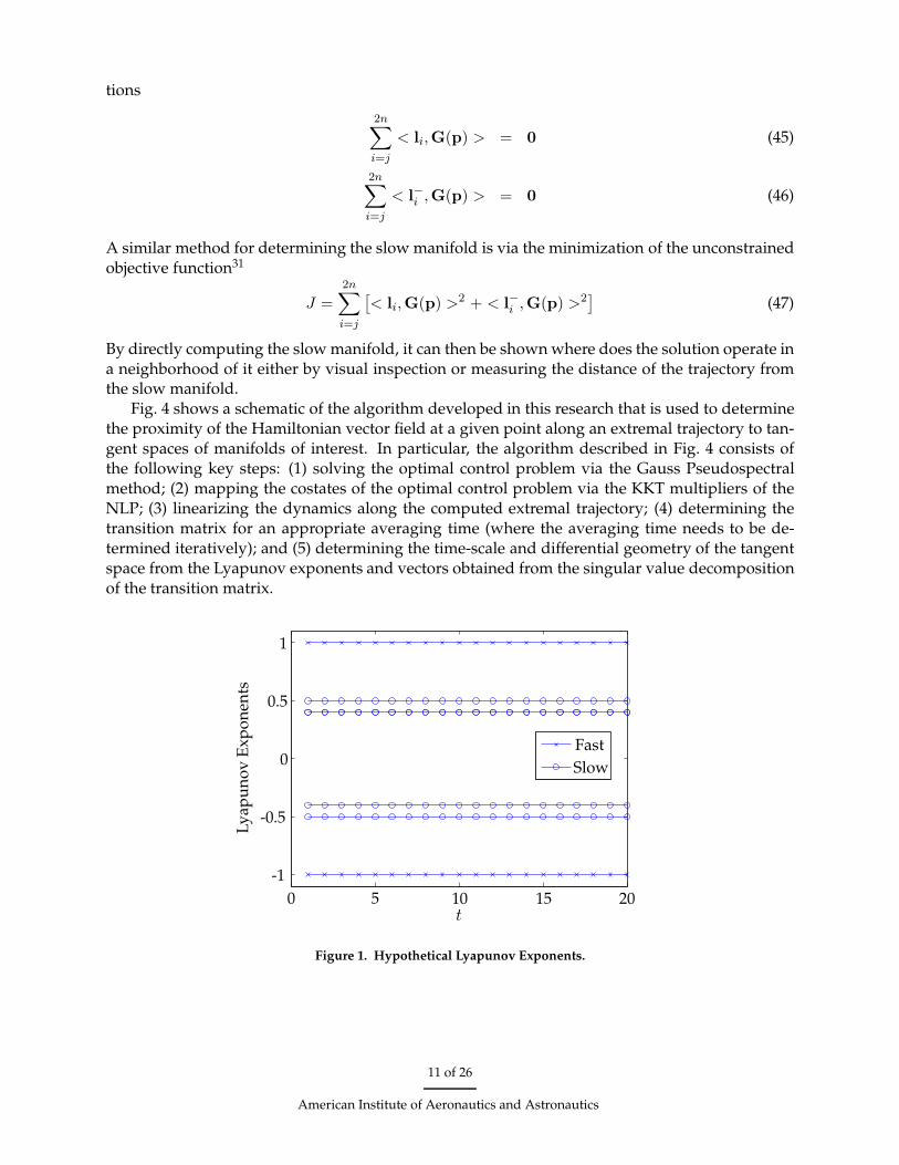
Note, if m = 2n, then P is the tangent vector expressed in the basis of Lyapunov vectors. Next,by analysis of the Lyapunov exponents, we can determine subspaces of interest. To understandbetter how the Lyapunov exponents can be used to determine relevant subspaces, consider thefollowing hypothetical example where t = 20 and n = 3 as shown in Fig. 1. It is observed for thishypothetical example that a significant separation exists between both the slow and fast exponentsand the stable and unstable exponents. There is not, however, a significant separation betweenthe slow-stable or slow-unstable exponents. The small spectral gap of 0.1 between the slow-stableand slow-unstable exponents shows that the averaging time t = 20 is not sufficiently long enoughto separate the slow-stable and slow-unstable behavior. A measure of the contribution of theHamiltonian vector field along the m vectors can then be determined by defining the distancemetric35

D(Pp,Pl) = ||Pp −Pl|| (40)

where Pp is the normalized phase space and Pl is a projection of the normalized phase space intoan arbitrary subspace defined above as P (i.e., the the fast-stable subspace, stable subspace, etc).

gThe expanding/contracting nature of Hamiltonian systems is a consequence of Liouville’s theorem34

9 of 26

American Institute of Aeronautics and Astronautics

Because we have normalized the phase space, the metric D returns a value between 0 ≤ D ≤ 1.The closer the tangent vector is to an arbitrary subspace, the closer Eq. (40) is to zero and the moreorthogonal the tangent vector is to an arbitrary subspace, the closer Eq. (40) is to one. Figs. 2 and 3provide schematics of the decomposition of a vector field in an arbitrary case and in a case wherethe vector field has a dominant stable component, respectively. In Fig. 2 it is seen that when Pstable

is subtracted from G(p), Pstable⊥ is large. Consequently, the value of the metric D is also large andthe tangent vector P(p) does not lie close to the tangent space of the stable manifold. On the otherhand, when Pstable⊥ is small (as shown in Fig. 3), the metric D will taken on a small value. As aresult, in this second case the tangent vector G(p) will lie close to the tangent space of the stablemanifold. In both cases, the notion of “close” depends upon a user-specified tolerance.

In general, the stable and unstable (or slow and fast) components of the tangent vector neednot be orthogonal to each other. Because a singular value decomposition of the transition matrixresults in an orthogonal set of vectors, only some of the resulting vectors will be aligned withthe corresponding directions of the different behaviors in the dynamical system. An approachfor increasing the number of correctly computed directions of either stable and unstable (or fastand slow) directions is to integrate the transition matrix in both forward and backward time. Thefollowing simple two-dimensional example31 (shown in more detail later), illustrates the need forbi-directional integration. In the neighborhood of an equilibrium point of a nonlinear dynamicalsystem, the Lyapunov exponents and vectors will converge to the eigenvalues and eigenvectors,which, in general, do not form an orthogonal basis. If a singular value decomposition is performedusing a forward integration of the transition matrix, one of the predicted finite-time Lyapunovvectors will be orthogonal. Because we know that the eigenvectors are correct, forward integrationis insufficient for obtaining the correct second direction. For this simple two-dimensional example,the approach would be to compute the stable Lyapunov vector in forward time (as described inRef. 31) and compute the unstable Lyapunov vector in backward time.

A method for capturing the fast-stable behavior in both forward and backward time alonga portion of the trajectory and determining if this portion of the trajectory is slow is given asfollows. The fast-stable components in forward and backward time are accurately computed byperforming a singular value decomposition of the transition matrix. Therefore, the collection offast stable vectors in forward time,

Lfs = (l1, l2, ...lm) (41)

and fast stable vectors in backward time,

L−fs = (l−

1, l−

2, ...l−m) (42)

define the fast stable and fast unstable directions, respectively, along the trajectory. The slowsubspace is defined as the intersection the subspaces up to and including the slow parts in forwardand backwards time, i.e.,

Lfs+slow ∩ L−fs+slow (43)

where Lfs+slow is the space spanned by the fast stable and slow directions. Then, instead of calcu-lating how close G(p) is to the tangent space to the slow manifold, the slow manifold is computeddirectly. In particular, the slow manifold, denoted S, can be found by computing where the tan-gent space to the non-linear dynamical system does not lie in S⊥. S⊥ is defined without proof(refer to Ref. 31 for proof) as

S⊥ = Lfu ⊕ L−fu (44)

where Lfu represents the space spanned by the fast unstable Lyapunov vectors (lj , lj+1, ..., l2n).Therefore, the slow manifold is reconstructed36 at points along the trajectory by solving the equa-

10 of 26

American Institute of Aeronautics and Astronautics

tions

2n∑

i=j

< li,G(p) > = 0 (45)

2n∑

i=j

< l−i ,G(p) > = 0 (46)

A similar method for determining the slow manifold is via the minimization of the unconstrainedobjective function31

J =

2n∑

i=j

[

< li,G(p) >2 + < l−i ,G(p) >2]

(47)

By directly computing the slow manifold, it can then be shown where does the solution operate ina neighborhood of it either by visual inspection or measuring the distance of the trajectory fromthe slow manifold.

Fig. 4 shows a schematic of the algorithm developed in this research that is used to determinethe proximity of the Hamiltonian vector field at a given point along an extremal trajectory to tan-gent spaces of manifolds of interest. In particular, the algorithm described in Fig. 4 consists ofthe following key steps: (1) solving the optimal control problem via the Gauss Pseudospectralmethod; (2) mapping the costates of the optimal control problem via the KKT multipliers of theNLP; (3) linearizing the dynamics along the computed extremal trajectory; (4) determining thetransition matrix for an appropriate averaging time (where the averaging time needs to be de-termined iteratively); and (5) determining the time-scale and differential geometry of the tangentspace from the Lyapunov exponents and vectors obtained from the singular value decompositionof the transition matrix.

t

-0.5

0

0

0.5

1

-1

5 10 15 20

Ly

apu

no

vE

xp

on

ents

Fast

Slow

Figure 1. Hypothetical Lyapunov Exponents.

11 of 26

American Institute of Aeronautics and Astronautics

Figure 2. Decomposition of G(p) into Components That Lie in the TangentSpace of the Stable Manifold and LieOrthogonal to the Tangent Space of the Stable Manifold.

Figure 3. Decomposition of G(p) into Components That Lie in the TangentSpace of the Stable Manifold and LieOrthogonal to the Tangent Space of the Stable Manifold for the Case Where the Dominant Behavior is Stable.

12 of 26

American Institute of Aeronautics and Astronautics

Transcribe Continuous Optimal ControlProblem to NLP via GPM

Map Solution of NLP to States & Costatesof Continuous Optimal Control Problem

Linearize Hamiltonian System Along PhaseSpace Trajectory Computing via GPM

Choose Reset Rate and ComputeTransition Matrix Along Optimal Trajectory

Guess Averaging Time and ComputeFinite-Time Lyapunov Exponents & Vectors

Analyze Time-Scalesand Differential Geometry

If Averaging Time is Adequate, Quit.Otherwise, Iterate on Averaging Time.

Figure 4. Solution to and Time-Scale Analysis for a General Nonlinear Optimal Control Problem.

13 of 26

American Institute of Aeronautics and Astronautics

VI. Example 1: Completely Hyper-sensitive Problem

Consider the following example adapted from Ref. 37. Minimize the quadratic cost functional

J =

∫ tf

0

(x2 + u2) dt (48)

subject to the dynamic constraintx = −x3 + u (49)

and the boundary conditions

x(0) = 1

x(tf ) = 1.5(50)

where the final time tf is fixed. The Hamiltonian is given as

H = x2 + u2 + λ(−x3 + u) (51)

Applying the first-order optimality conditions from the calculus of variations leads to the follow-ing Hamiltonian boundary-value problem:

x = Hλ = −x3 − λ/2 , x(0) = 1

λ = −Hx = −2x + 3x2λ , x(tf ) = 1.5(52)

It is known that, for sufficiently large values of tf , the optimal control problem of Eqs. (48)–(50) ishyper-sensitive37 because the time interval over which the problem is solved is significantly longerthan the minimum rate of contraction and expansion of the Hamiltonian system in the neighbor-hood of the optimal solution.27, 37 Moreover, extremal trajectories of the optimal control problem ofEqs. (48)–(50) take on the following three-segment structure as tf increases: (1) a rapidly decayingsegment that lies along the stable manifold of the equilibrium point of the Hamiltonian system;(2) a slow segment that lies close to the equilibrium point; and (3) a rapidly growing segment thatgrows to meet the terminal boundary condition.

In order to demonstrate the hyper-sensitivity, this problem was solved using the Gauss pseu-dospectral method for 50 nodes using the TOMLAB R©38 version of the NLP solver SNOPT.6 Be-cause this problem has a two-dimensional Hamiltonian phase space, the hyper-sensitivity can beinferred graphically. First, the evolution of the solution in time is seen in Fig. 5 where the three-segment structure is apparent due to the exponential-like behaviors at the ends with a constantsegment in the middle. Furthermore, examining Fig. 7, it is seen that the solution in the phasespace looks like two curves connected by a “kink”. As it turns out, the curve emanating fromthe initial condition and ending at the kink is a segment of the stable manifold while the segmentstarting at the kink and ending at the terminal condition is a segment of the unstable manifold.

Suppose now that one was to assess the structure of the problem, but without any knowledgea priori of the hyper-sensitivity. In this case, suppose we apply the aforementioned frameworkthat uses Lyapunov exponents and vectors to deduce differential geometry. For this problem,computation of the finite time Lyapunov exponents and vectors was conducted with an averagingtime of 3 and a reset time on the transition matrix of 0.25 h. Using the Hamiltonian system ofEq. (52), a comparison is made between the identification of directions corresponding the stableand unstable behavior using the eigenvectors of the Jacobian and using a decomposition based on

hTo reduce accumulation of numerical errors, the transition matrix is solved for smaller steps, and then these aremultiplied together to give the transition matrix over the desired averaging time.

14 of 26

American Institute of Aeronautics and Astronautics

x

t

00

0.5

1

1.5

5 10 15 20 25

Figure 5. x(t) vs. t for Completely Hyper-Sensitive Problem.

the finite-time Lyapunov vectors. Because the initial part of the trajectory lies extremely close tothe stable manifold, it is known that the vector field G(p) is aligned essentially with the tangentspace to the stable manifold (see Ref. 37 for details). The fact that G(p(0)) lies along the tangentspace to the stable manifold is seen in Fig. 8 where G(p(0)) is tangent to the phase space trajectory.Moreover, because of the known direction of G(p(0)), any basis that properly identifies the stabledirection should have a direction that is tangent to the trajectory at t = 0. Examining Fig. 8 itis seen that one of the finite-time Lyapunov vectors indeed lies in the same direction as G(p(0)).Contrariwise, while one of the eigenvectors of [∂G/∂p]t=0

lies in a direction that is somewhataligned with G(p(0)), it is seen that this eigenvector is not nearly as good an indicator of thestable behavior as is the stable finite-time Lyapunov vector. Fig. 9 shows that during the initialsegment (the green portion which ends at approximately 5), the tangent space to the vector fieldaligns well with the stable Lyapunov vector. This is expected as the initial segment should operatein close proximity to the stable manifold. At the equilibrium point (the blue portion), the trajectorybegins to leave its alignment with the stable Lyapunov vector. Similar results hold for the unstablesegment utilizing the backwards time stable Lyapunov vector. Next, Fig. 8 shows a decomposi-tion of the tangent vector at a point p that lies extremely close to the hyperbolic equilibrium point,p = (0, 0), of the Hamiltonian system of Eq. (52). As expected, because the equilibrium pointis hyperbolic,39 the eigenvectors accurately identify both the stable and unstable directions in theneighborhood of p. Contrariwise, it is seen that the stable finite-time Lyapunov vector provides re-liable information whereas unstable finite-time Lyapunov vector is not reliable. The reason in thissecond case that the supposed “unstable” Lyapunov vector lies in a direction that is incongruentwith the direction of unstable motion is because the singular-value decomposition was computedusing a transition matrix that was obtained via a forward time integration of the linearized dynam-ics. It has been recently discussed (see Ref. 31) that using forward integration alone is generallyinadequate in identifying all of the constituent time-scales and stability (i.e., backward integra-

15 of 26

American Institute of Aeronautics and Astronautics

λ

t

0

0

-5

-10

-15

5

5 10 15 20 25

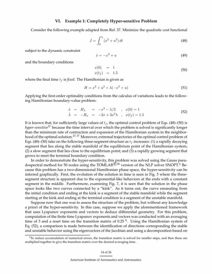
Figure 6. λ(t) vs. t for Completely Hyper-Sensitive Problem.

tion is also needed). The issue of forward/backward propagation to identify all of the constituentbehaviors is a concept that has come to the attention of the authors only recently (see Ref. 31 forsome background on this topic) and is a topic of ongoing research.

Next, using the finite-time Lyapunov exponents, the time-scales can be obtained. Fig. 10 showsthe stable and unstable Lyapunov exponents for this problem at various point along the trajectory.It is seen that the Lyapunov exponents converge to approximately ±1, indicating that the time-scales are close to unity. Interestingly, the Jacobian of the Hamiltonian system for this problem isgiven as

∂G

∂p=

[

−3x2 −1/2

−2 + 6xλ 3x2

]

(53)

Evaluating the eigenvalues of the Jacobian at the equilibrium point p = (0, 0), we obtain ±1 (thusindicating that the time-scales are unity in the neighborhood of the equilibrium point). Becausewe expect that the time-scales will change gradually as we move away from the equilibrium point,we expect the time-scales to remain somewhat close to unity along the optimal trajectory. Indeed,in this case the finite-time Lyapunov exponents are consistent with the expected result.

16 of 26

American Institute of Aeronautics and Astronautics

Equilibrium Point

Stable Manifold

Unstable Manifold

x

λ0

0 0.5 1 1.5

-5

-10

-15

5

Figure 7. λ vs. x for Completely Hyper-Sensitive Problem.

x

λ

-1.5

-0.5

0

0

0.5

1

1

1.5

-1

-1

2

2 3

G(p)

Lyapunov

Eigenvectors

Figure 8. Comparison of Lyapunov Vectors and Eigenvectors (CHSP).

17 of 26

American Institute of Aeronautics and Astronautics

‖G(p

)−

Pst

able‖

t

00

0.1

0.2

0.3

0.4

0.5

2 4 6 8 10

Figure 9. Alignment of the Stable manifold with the Stable Lyapunov Vector for the Completely Hyper-SensitiveProblem.

t

-1.5

-0.5

0

0

0.5

1

1.5

-1

5 10 15 20

Ly

apu

no

vE

xp

on

ents

Figure 10. Lyapunov Exponents along the Trajectory for the Completely Hyper-Sensitive Problem.

18 of 26

American Institute of Aeronautics and Astronautics

VII. Example 2: Chemical Reaction Problem

Consider the following optimal control problem taken from Ref. 20. Minimize the cost func-tional

J =

∫ tf

0

(x4 + 1

2z2 + 1

2u2) dt (54)

subject to the dynamic constraints

x = xz

z = ρ(−z + u)

(55)

and the boundary conditions

x0 =√

2/2

x(tf ) = 1/2

z0 = 0

z(tf ) = 0

tf = 1

(56)

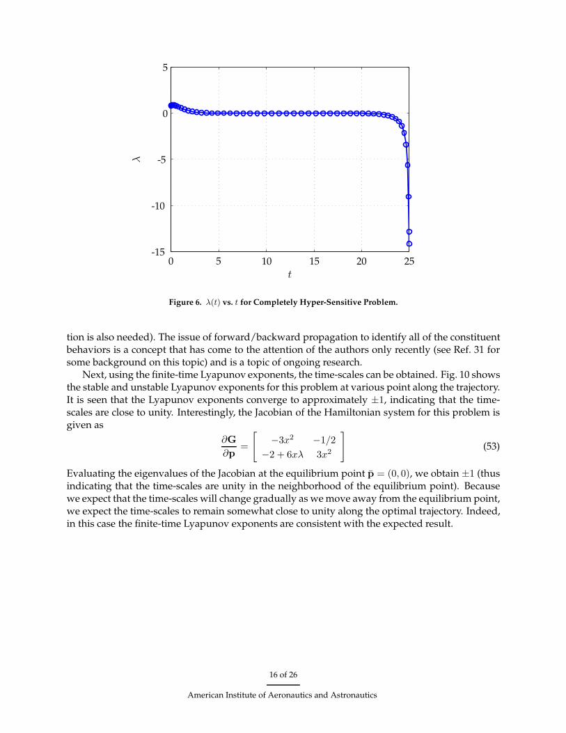
As stated, the optimal control problem of Eqs. (54)–(56) is in the standard singularly perturbedformi with x and z being the slow and fast variables, respectively. The optimal trajectory forρ = 10 is shown in Fig. 11. It is seen that the variable z takes on a three-segment structure witha rapid initial decay from the initial condition, a slow middle segment, and a rapid rise to meetthe terminal conditions. What is also seen is that x remains slow throughout the trajectory, whichis expected as it is the slow variable. Analyzing the time-scales, Fig. 12 shows the finite-timeLyapunov exponents for ρ = (10, 15, 20) using an averaging time t = 0.5 and a transition matrixreset time of 0.02. It is seen that the slow Lyapunov exponents (i.e., the red curves marked withdiamonds in Fig. 12) do not change significantly as ρ is increased. The slow Lyapunov exponentsare actually indistinguishable for each value of ρ. On the other hand, the fast Lyapunov exponents(i.e., the blue curves with circles) do change significantly with increasing ρ. This behavior in theslow and fast Lyapunov exponents is expected because the dynamics of the variable x remainunchanged as ρ is changed while the dynamics of the variable z increase in speed as ρ increases.While it may seem that a final time of tf = 1 is small and, thus, should not elicit a time-scaleseparation in the solution, the fast time-scale in this problem for ρ ≫ 1 is sufficiently smallerthan unity and thus, a time-scale separation appears in the solution. Fig. 13 shows z(t) alongsidethe slow manifold where the slow manifold is calculated by setting to zero the component of theHamiltonian vector field in the direction of the fast-unstable Lyapunov vector (where the fast-unstable Lyapunov vectors are computed via both forward and backward integration). The slowmanifold was calculated by fixing x and λx to their values from the GPM solution and solvingfor z and λz . It is seen that the solution for z(t) lies in the slow manifold in the middle segment,consistent with the fact that a time-scale separation exists and z is the fast variable.

Suppose now that this problem was cast in a form that did not explicitly identify the slow andfast motion (i.e., the problem was not posed in the standard singularly perturbed form). In this caseidentifying the slow manifold would be less straightforward than was done in the aforementionedanalysis. In order to see how one might identify the time-scales for this problem when given thedynamics in a non-standard form, consider the following underdetermined relationship betweenthe variables x, y, and z:

x = y2 + z (57)

iThe standard singularly perturbed form is obtained by setting ǫ = 1/ρ in the second differential equation.

19 of 26

American Institute of Aeronautics and Astronautics

t

-0.5

0

0 0.2 0.4

0.5

0.6 0.8

1

1

x

x

z

Figure 11. States x and z vs. Time (ρ = 10) for Chemical Reaction Example.

Using Eq. (57), the following two new sets of differential equations can be derived:

x = x2 − xy

y =x2 − xy2

2y− ρ(−x + y2 + u)

2y

(58)

and

y =y2z + z2

2y− ρ(−z + u)

2y

z = ρ(−z + u)

(59)

The cost functionals corresponding to Eqs. (58) and (59) are given, respectively, as

J =

∫

1

0

(x4 + 1

2(x − y2)2 + 1

2u2) dt (60)

J =

∫

1

0

((y2 + z)4 + 1

2z2 + 1

2u2) dt (61)

It is noted that, for the case of the (y, z) dynamics, no explicit time-scale separation exists betweeny and z.

To analyze how the state space models (x, y) and (y, z) compare to the standard singularlyperturbed form (x, z) each problem was solved by the GPM. The optimal trajectories for the (x, z),(x, y) and (y, z) systems is shown in Fig. 11 for 50 LG points with ρ = 10 (where the relationshipof Eq. 57 was used to change between variables when appropriate). The slow manifold was then

20 of 26

American Institute of Aeronautics and Astronautics

t

0

0

-20

-405 10 15

20

20 25

40

Ly

apu

no

vE

xp

on

ents

ρ = 10 ρ = 15 ρ = 20

Figure 12. Lyapunov Exponents vs. Time for ρ = (10, 15, 20) for Chemical Reaction Problem.

calculated with each state variable representation. Then, using Eq. (57), the slow manifold wascomputed in terms of z. Figs. 14 and 15 show the slow manifold for the (x, y) and (y, z) repre-sentations, respectively, in terms of the variable z. What is seen is that in both the (x, y) and (y, z)cases, the slow manifold is comparable to the one produced from the singularly perturbed form.

It should be noted that all the above slow manifolds were generated using an averaging time of0.02 to calculate the Lyapunov vectors. As the averaging time increases, the range over which theslow manifold can be calculated shrinks because forward and backwards time are being analyzedsimultaneously. For example, for a trajectory of duration 10 time unit and an averaging time of1 time unit in forward time, the last possible time where the Lyapunov vector can be calculatedis at 9 time units because for anytime beyond 9 time units the calculation of a Lyapunov vectorwill require information beyond the terminal time of the trajectory. In this example, the rangeover which slow manifold can be analyzed would be from 1 to 9 time units (because in backwardstime the last vector is calculated at 1 time unit). No appreciable difference was noticed betweenthe slow manifold calculated with a longer averaging time than one which was calculated with ashort one, so the shortest averaging time was used.

21 of 26

American Institute of Aeronautics and Astronautics

t

t

t

-0.5

-0.5

-0.5

0

0

0

0

0

0

0.2

0.2

0.2

0.4

0.4

0.4

0.6

0.6

0.6

0.8

0.8

0.8

1

1

1

z(ρ

=10

)z

(ρ=

15)

z(ρ

=20

)

Figure 13. Slow Manifold for the Chemical Reaction Problem for ρ = (10, 15, 20) Using the Standard SingularlyPerturbed Form.

22 of 26

American Institute of Aeronautics and Astronautics

t

t

t

-0.5

-0.5

-0.5

0

0

0

0

0

0

0.2

0.2

0.2

0.4

0.4

0.4

0.6

0.6

0.6

0.8

0.8

0.8

1

1

1

z(ρ

=10

)z

(ρ=

15)

z(ρ

=20

)

Figure 14. Slow Manifold for the Chemical Reaction Example for ρ = 10,15,20 Using the (x, y) Representation of theDynamics.

23 of 26

American Institute of Aeronautics and Astronautics

t

t

t

-0.2

-0.2

-0.2

-0.4

-0.4

-0.4

0

0

0

0

0

0

0.2

0.2

0.2

0.4

0.4

0.4

0.6

0.6

0.6

0.8

0.8

0.8

1

1

1

z(ρ

=10

)z

(ρ=

15)

z(ρ

=20

)

Figure 15. Slow Manifold for the Chemical Reaction Example for ρ = 10,15,20 Using the (y, z) Representation of theDynamics.

24 of 26

American Institute of Aeronautics and Astronautics

VIII. Conclusions

An initial examination has been performed into using pseudospectral methods to infer time-scale and differential geometric structure in nonlinear optimal control problems. In particular,the Gauss pseudospectral method has been used to generate accurate Hamiltonian phase spacetrajectories. These phase space trajectories were then analyzed using a computational differen-tial geometric approach where finite-time Lyapunov exponents and vectors have been computedalong the extremal trajectory. The active time-scales and stability has then been determined byexamining the dominant direction of the Hamiltonian vector field along the extremal trajectory.The results obtained in this study provide a starting point for time-scale and differential geometricanalysis of nonlinear optimal control problems and show the utility of the Gauss pseudospectralmethod as a viable computational engine to conduct such analysis.

IX. Acknowledgments

The authors gratefully acknowledge support for this research under funding from The Uni-versity of Florida.

References

1Betts, J. T., Practical Methods for Optimal Control Using Nonlinear Programming, SIAM, 2001.2Keller, H. B., Numerical Solution of Two Point Boundary Value Problems, SIAM, 1976.3Oberle, H. J. and Grimm, W., “BNDSCO: A Program for the Numerical Solution of Optimal Control Problems,”

Tech. rep., Institute of Flight Systems Dynamics, German Aerospace Research Establishment DLR, Oberpfaffenhofen,Germany, 1989.

4Stoer, J. and Bulirsch, R., Introduction to Numerical Analysis, Springer-Verlag, 2002.5Kirk, D. E., Optimal Control Theory: An Introduction, Dover Publications, 2004.6Gill, P. E., Murray, W., and Saunders, M. A., User’s Guide for SNOPT Version 7: Software for Large Scale Nonlinear

Programming, February 2006.7Holmstrom, K., Goran, A. O., and Edvall, M. M., User’s Guide for Tomlab / Knitro v5.1, April 2007.8Holmstrom, K., Goran, A. O., and Edvall, M. M., User’s Guide for Tomlab / SPRNLP / BARNLP, November 2006.9Bazaraa, M. S., Sherali, H. D., and Shetty, C. M., Nonlinear Programming: Theory and Algorithms, Wiley-

Interscience, 3rd ed., 2006.10Elnagar, G., Kazemi, M., and Razzaghi, M., “The Pseudospectral Legendre Method for Discretizing Optimal

Control Problems,” IEEE Transactions on Automatic Control, Vol. 40, No. 10, 1995, pp. 1793–1796.11Fahroo, F. and Ross, I. M., “Costate Estimation by a Legendre Pseudospectral Method,” Journal of Guidance,

Control, and Dynamics, Vol. 24, No. 2, 2001, pp. 270–277.12Huntington, G. T. and Rao, A. V., “A Comparison of Accuracy and Computational Efficiency of Three Pseu-

dospectral Methods,” Proceedings of Guidance, Navigation and Control Conference, AIAA Paper 2007-6405, Hilton Head,South Carolina, August 2007.

13Kameswaran, S. and Biegler, L. T., “Convergence Rates for Direct Transcription of Optimal Control ProblemsUsing Collocation at Radau Points,” Computation Optimization and Applications, Vol. 41, No. 1, 2008, pp. 81–126.

14Benson, D. A., A Gauss Pseudospectral Transcription for Optimal Control, Ph.D. thesis, MIT, 2004.15Benson, D. A., Huntington, G. T., Thorvaldsen, T. P., and Rao, A. V., “Direct Trajectory Optimization and Costate

Estimation via an Orthogonal Collocation Method,” Journal of Guidance, Control, and Dynamics, Vol. 29, No. 6, November-December 2006, pp. 1435–1440.

16Huntington, G. T., Advancement and Analysis of a Gauss Pseudospectral Transcription for Optimal Control, Ph.D. thesis,Department of Aeronautics and Astronautics, Massachusetts Institute of Technology, 2007.

17Huntington, G. T., Benson, D. A., and Rao, A. V., “Optimal Configuration of Tetrahedral Spacecraft Formations,”The Journal of the Astronautical Sciences, Vol. 55, No. 2, April-June 2007, pp. 141–169.

25 of 26

American Institute of Aeronautics and Astronautics

18Huntington, G. T. and Rao, A. V., “Optimal Reconfiguration of Spacecraft Formations Using the Gauss Pseu-dospectral Method,” Journal of Guidance, Control, and Dynamics, Vol. 31, No. 3, May-June 2008, pp. 689–698.

19Huntington, G. T., Benson, D. A., How, J. P., Kanizay, N., Darby, C. L., and Rao, A. V., “Computation of End-point Controls Using a Gauss Pseudospectral Method,” Astrodynamics Specialist Conference, Mackinac Island, Michigan,August 2007.

20Kokotovic, P. V., Khalil, H. K., and O’Reilly, J., Singular Perturbation Methods in Control: Analysis and Design,Academic Press Inc., 1986.

21Hinch, E. J., Perturbation Methods, Cambridge University Press, 1991.22Lam, S. H., “Using CSP to Understand Complex Chemical Kinetics,” Comb. Science Tech, Vol. 89, 1993, pp. 375–

404.23Lam, S. H. and Goussis, D. A., “The CSP Method of Simplifying Kinetics,” Int. J. Chem. Kin., Vol. 26, 1994,

pp. 461–486.24Lam, S. H., Goussis, D. A., and Konopka, D., “Time-Resolved Simplified Chemical Kinetics Modeling Using

Computation Singular Perturbation,” AIAA 27th Aerospace Sciences Meeting (AIAA 89-0575), Reno, Nevada, January1989.

25Rao, A. V. and Mease, K. D., “A New Method for Solving Optimal Control Problems,” Proceedings of the AIAAGuidance, Navigation and Control Conference, Baltimore, 1995, pp. 818–825.

26Rao, A. V., Extension of the Computational Singular Perturbation Method to Optimal Control, Ph.D. thesis, PrincetonUniversity, 1996.

27Topcu, U. and Mease, K. D., “Using Lyapunov Vectors and Dichotomy to Solve Hyper-Sensitive Optimal ControlProblems,” Proceedings of the 45th IEEE Conference on Decision and Control, 2006.

28Mease, K. D., Bharadwaj, S., and Iravanchy, S., “Timescale Analysis for Nonlinear Dynamical Systems,” Journalof Guidance, Control and Dynamics, Vol. 26, No. 2, March-April 2003, pp. 318–330.

29Lyapunov, A. M., “The General Problem of Stability of Motion,” International Journal of Control, Vol. 55, No. 3,1992, pp. 531–773.

30Lorenz, E. N., “The Local Structure of a Chaotic Attractor in Four-Dimensions,” Physica D, Vol. 13D, No. 1-2,1984, pp. 90–104.

31Mease, K. D., Topcu, U., and Aykutlug, E., “Characterizing Two-Timescale Nonlinear Dynamics Using Finite-Time Lyapunov Exponents and Vectors,” ArXiv.org, July 2008, pp. 318–330.

32Dahlquist, G. and Bjorck, A., Numerical Methods, Dover Publications, 2003.33Trefethen, L. N. and David Bau, I., Numerical Linear Algebra, SIAM, 1997.34Arnol’d, V. I., Dynamical Systems, Vol. 5, Springer, 1991.35Hoffman, K. and Kunze, R., Linear Algebra, Prentice-Hall, Inc., 2nd ed., 1971.36Iravanchy, S., Computational Methods for Time-Scale Analysis of Nonlinear Dynamical Systems, Ph.D. thesis, Univer-

sity of California, Irvine, 2003.37Rao, A. V. and Mease, K. D., “Eigenvector Approximate Dichotomic Basis Method for Solving Hyper-Sensitive

Optimal Control Problems,” Optimal Control Applications and Methods, 2000.38Holmstrom, K., Goran, A. O., and Edvall, M. M., User’s Guide for Tomlab, November 2007.39Guckenheimer, J. and Holmes, P. J., Nonlinear Oscillations, Dynamical Systems, and Bifurcations of Vector Fields,

Springer-Verlag, New York, 1990.

26 of 26

American Institute of Aeronautics and Astronautics