1 An Efficient Overloaded Method for Computing Derivatives...
39
1 An Efficient Overloaded Method for Computing Derivatives of Mathematical Functions in MATLAB Michael A. Patterson, University of Florida Matthew Weinstein, University of Florida Anil V. Rao, University of Florida An object-oriented method is presented that computes without truncation error derivatives of functions defined by MATLAB computer codes. The method implements forward mode automatic differentiation via operator overloading in a manner that produces a new MATLAB code which computes the derivatives of the outputs of the original function with respect to the variables of differentiation. Because the derivative code has the same input as the original function code, the method can be used recursively to generate derivatives of any order that are desired. In addition, the approach developed in this paper has the feature that the derivatives are generated simply by evaluating the function on an instance of the class, thus making the method straightforward to use while simultaneously enabling differentiation of highly complex functions. A detailed description of the method is presented and the approach is illustrated and is shown to be efficient on four examples. Categories and Subject Descriptors: G.1.4 [Numerical Analysis]: Automatic Differentiation General Terms: Automatic Differentiation, Numerical Methods, MATLAB. Additional Key Words and Phrases: Scientific Computation, Applied Mathematics. ACM Reference Format: Patterson, M. A., Weinstein, M., and Rao, A. V. 2010. An efficient overloaded method for computing deriva- tives of mathematical functions in MATLAB. ACM Trans. Math. Soft. 39, 3, Article 1 (July 2013), 39 pages. DOI = 10.1145/0000000.0000000 http://doi.acm.org/10.1145/0000000.0000000 1. INTRODUCTION Obtaining accurate approximations to derivatives of general functions is important in a variety of subjects including science, engineering, economics, and scientific com- putation. Derivative approximation techniques fall into three general categories: nu- merical approximation, symbolic differentiation, and automatic differentiation. Nu- merical approximation techniques include the classical methods of finite-differencing (e.g., forward and central differencing) and the complex-step derivative approximation [Martins et al. 2003]. In the case of finite-differencing, the derivative is replaced by a computation where the function is evaluated at two neighboring values of the ordinate The authors gratefully acknowledge support for this research from the U.S. Office of Naval Research (ONR) under Grant N00014-11-1-0068 and from the U.S. Defense Advanced Research Projects Agency (DARPA) Under Contract HR0011-12-0011. The authors would also like to thank the Referees for improving the manuscript through their thoughtful and constructive reviews. Disclaimer: The views expressed are those of the authors and do not reflect the official policy or position of the Department of Defense or the U.S. Gov- ernment. Author’s addresses: M. A. Patterson, M. Weinstein, and A. V. Rao, Department of Mechanical and Aerospace Engineering, P.O. Box 116250, University of Florida, Gainesville, FL 32611-6250; e-mail: {mpat- terson,mweinstein,anilvrao}@ufl.edu. Permission to make digital or hard copies of part or all of this work for personal or classroom use is granted without fee provided that copies are not made or distributed for profit or commercial advantage and that copies show this notice on the first page or initial screen of a display along with the full citation. Copyrights for components of this work owned by others than ACM must be honored. Abstracting with credit is per- mitted. To copy otherwise, to republish, to post on servers, to redistribute to lists, or to use any component of this work in other works requires prior specific permission and/or a fee. Permissions may be requested from Publications Dept., ACM, Inc., 2 Penn Plaza, Suite 701, New York, NY 10121-0701 USA, fax +1 (212) 869-0481, or [email protected]. © 2013 ACM 1539-9087/2013/07-ART1 $15.00 DOI 10.1145/0000000.0000000 http://doi.acm.org/10.1145/0000000.0000000 ACM Transactions on Mathematical Software, Vol. 39, No. 3, Article 1, Publication date: July 2013.
Transcript of 1 An Efficient Overloaded Method for Computing Derivatives...

1
An Efficient Overloaded Method for Computing Derivatives ofMathematical Functions in MATLAB
Michael A. Patterson, University of FloridaMatthew Weinstein, University of FloridaAnil V. Rao, University of Florida
An object-oriented method is presented that computes without truncation error derivatives of functionsdefined by MATLAB computer codes. The method implements forward mode automatic differentiation viaoperator overloading in a manner that produces a new MATLAB code which computes the derivatives of theoutputs of the original function with respect to the variables of differentiation. Because the derivative codehas the same input as the original function code, the method can be used recursively to generate derivativesof any order that are desired. In addition, the approach developed in this paper has the feature that thederivatives are generated simply by evaluating the function on an instance of the class, thus making themethod straightforward to use while simultaneously enabling differentiation of highly complex functions. Adetailed description of the method is presented and the approach is illustrated and is shown to be efficienton four examples.
Categories and Subject Descriptors: G.1.4 [Numerical Analysis]: Automatic Differentiation
General Terms: Automatic Differentiation, Numerical Methods, MATLAB.
Additional Key Words and Phrases: Scientific Computation, Applied Mathematics.
ACM Reference Format:Patterson, M. A., Weinstein, M., and Rao, A. V. 2010. An efficient overloaded method for computing deriva-tives of mathematical functions in MATLAB. ACM Trans. Math. Soft. 39, 3, Article 1 (July 2013), 39 pages.DOI = 10.1145/0000000.0000000 http://doi.acm.org/10.1145/0000000.0000000
1. INTRODUCTION
Obtaining accurate approximations to derivatives of general functions is importantin a variety of subjects including science, engineering, economics, and scientific com-putation. Derivative approximation techniques fall into three general categories: nu-merical approximation, symbolic differentiation, and automatic differentiation. Nu-merical approximation techniques include the classical methods of finite-differencing(e.g., forward and central differencing) and the complex-step derivative approximation[Martins et al. 2003]. In the case of finite-differencing, the derivative is replaced by acomputation where the function is evaluated at two neighboring values of the ordinate
The authors gratefully acknowledge support for this research from the U.S. Office of Naval Research (ONR)under Grant N00014-11-1-0068 and from the U.S. Defense Advanced Research Projects Agency (DARPA)Under Contract HR0011-12-0011. The authors would also like to thank the Referees for improving themanuscript through their thoughtful and constructive reviews. Disclaimer: The views expressed are thoseof the authors and do not reflect the official policy or position of the Department of Defense or the U.S. Gov-ernment.Author’s addresses: M. A. Patterson, M. Weinstein, and A. V. Rao, Department of Mechanical andAerospace Engineering, P.O. Box 116250, University of Florida, Gainesville, FL 32611-6250; e-mail: {mpat-terson,mweinstein,anilvrao}@ufl.edu.Permission to make digital or hard copies of part or all of this work for personal or classroom use is grantedwithout fee provided that copies are not made or distributed for profit or commercial advantage and thatcopies show this notice on the first page or initial screen of a display along with the full citation. Copyrightsfor components of this work owned by others than ACM must be honored. Abstracting with credit is per-mitted. To copy otherwise, to republish, to post on servers, to redistribute to lists, or to use any componentof this work in other works requires prior specific permission and/or a fee. Permissions may be requestedfrom Publications Dept., ACM, Inc., 2 Penn Plaza, Suite 701, New York, NY 10121-0701 USA, fax +1 (212)869-0481, or [email protected].© 2013 ACM 1539-9087/2013/07-ART1 $15.00DOI 10.1145/0000000.0000000 http://doi.acm.org/10.1145/0000000.0000000
ACM Transactions on Mathematical Software, Vol. 39, No. 3, Article 1, Publication date: July 2013.

1:2 M. A. Patterson, M. Weinstein, and A. V. Rao
and the difference between these function values is divided by the difference in the or-dinate values. Great care must be taken in finite-differencing because ordinate valuesthat are too widely spaced lead to an inaccurate derivative while ordinate values thatare too closely spaced can result in catastrophic cancellation in the numerator of theapproximation. In the complex-step derivative approximation [Martins et al. 2003], theperturbation is taken in the imaginary direction in the complex plane. The complex-step derivative approximation has a useful feature that the derivative can be approx-imated without taking the difference between two values of the function. Instead, byperturbing the ordinate in the imaginary direction, it is possible to make the pertur-bation size extremely small and obtain a highly accurate derivative approximation.Unlike finite-differencing, the complex-step derivative approximation does not sufferfrom catastrophic cancellation when extremely small perturbation sizes are used. Itis noted that a more general version of the complex-step derivative approximation,called the multi-complex-step derivative approximation [Lantoine et al. 2012] has beendeveloped to obtain approximations to higher-order derivatives. Finally, the softwarePMAD [Shampine 2007] is a MATLAB implementation of the complex-step derivativeapproximation.
A second differentiation approach that is available as part of a more general com-puter algebra system, is symbolic differentiation. Symbolic differentiation is performedusing symbolic representations of the actual quantities or variables being manipulatedand is essentially a way of programming a computer to perform the steps that a hu-man would perform by hand. Symbolic differentiation is most often implemented byaccumulating the function into a single expression and differentiating the expressionusing defined rules of algebra and calculus. While symbolic differentiation is appeal-ing, it can become computationally difficult for very large problems due to the possibleexplosion in expression size that can arise when computing the derivatives of a com-plicated function. Many software programs that implement symbolic differentiationare available today including MAPLE [Monagan et al. 2005], Mathematica [Wolfram2008], and the MATLAB Symbolic Toolbox [Mathworks 2010].
In the past few decades, a great deal of research has focused on automatic differ-entiation (AD). AD is the process of determining accurate derivatives of a functiondefined by computer programs [Griewank 2008] using the rules of differential calcu-lus. In other words, the goal of AD is to employ ordinary calculus algorithmically withthe goal of obtaining machine precision accuracy derivatives in a computationally ef-ficient manner. AD exploits the fact that a computer code that implements a generalfunction y = f(x) can be decomposed into a sequence of elementary function opera-tions. The derivative is then obtained by applying the standard differentiation rules(e.g., product, quotient, and chain rules).
The most well known methods for automatic differentiation are forward and reversemode. In either forward or reverse mode, each link in the calculus chain rule is im-plemented until the derivative of the input with respect to itself is encountered. Thefundamental difference between forward and reverse modes is the direction in whichthe operations are performed. In forward mode, the operations are performed from thevariable of differentiation to the final derivative of the function, while in reverse modethe operations are performed from the function back to the variable of differentiation.
Forward and reverse mode automatic differentiation are implemented using eitheroperator overloading or source transformation. In an operator-overloaded approach,a custom class is constructed and all standard arithmetic operations and mathemat-ical functions are defined to operate on objects of the class. Furthermore, any objectof the custom class typically contains properties that include the value and first- orhigher-order derivatives of the object at a particular numerical value of the input.The process of forward mode automatic differentiation begins with an instance of the
ACM Transactions on Mathematical Software, Vol. 39, No. 3, Article 1, Publication date: July 2013.

An Efficient Overloaded Method for Computing Derivatives in MATLAB 1:3
class (for which the instance of the class represents the identity matrix). The deriva-tives are then propagated through each overloaded operation and function call, andthe derivative of the output with respect to the input is obtained at the numericalvalue contained in the value property of the instantiated object. In a source trans-formation approach, the original source code is replaced by a new code such that thenew code contains statements that compute the derivatives, and these new lines ofcode are interleaved with the statements in the original code. Well known implemen-tations of forward and reverse mode that utilize operator overloading include ADMIT-1[Coleman and Verma 1998b], ADMAT [Coleman and Verma 1998a], INTLAB [Rump1999], ADOL-C [Griewank et al. 1996], and MAD [Forth 2006], while well known im-plementations of source transformation include ADIFOR [Bischof et al. 1992; Bischofet al. 1996], PCOMP [Dobmann et al. 1995], TAPENADE [Hascoët and Pascual 2004],AdiMat [Bischof et al. 2002], and MSAD [Kharche and Forth 2006]. Amongst thesepreviously developed source transformation tools, the programs AdiMat [Bischof et al.2002] and MSAD [Kharche and Forth 2006] are designed to return MATLAB codethat computes the derivative of the original function [Neidinger 2010]. AdiMat uti-lizes a hybrid source transformation and operator-overloading approach to implementthe forward mode [Bischof et al. 2002]. AdiMat computes single directional derivatives,however, computing multiple directional derivatives require the use of a MATLAB mexinterface [Kharche 2011]. MSAD [Kharche and Forth 2006] combines source transfor-mation with with the efficient data structures in MAD [Forth 2006], resulting in ahybrid source transformation/operator overloading approach similar to that found inAdiMat [Bischof et al. 2002]. Ref. Kharche and Forth [2006] provides a description ofMSAD and demonstrates the effectiveness of MSAD on several test cases.
In this paper we present a new approach for automatic differentiation of MATLABcode. The method of this paper combines features of operator-overloading and sourcetransformation together with forward mode automatic differentiation in a manner thatproduces a new MATLAB code that contains statements to compute the derivative ofthe original MATLAB function in terms of the native MATLAB library. In order to re-alize our approach, a new MATLAB object class, called CADA (where CADA stands for“Computation of Analytic Derivatives Automatically”), is developed. Using instancesof class CADA, the function is evaluated on the input CADA object. CADA then pro-duces a file that contains the statements that compute the derivative of the originalfunction with respect to the input variable. The sequence of mathematical operationsin the file that computes the derivative file is identical to those obtained by applyingthe forward mode on a numeric value of the variable of differentiation.
As stated, the approach developed in this paper differs from previously developedautomatic differentiation methods in that it is neither purely a traditional operatoroverloaded method nor purely a source transformation tool. Instead, the approachcombines features of operator overloading and source transformation in that an object-oriented approach is used to generate a new code that contains the derivatives of theoriginal code. The similarity with an operator overloading approach lies in the fact thatthe method also uses operator overloading. The method of this paper, however, does notuse operator overloading in the same manner as is used by other operator overloadedautomatic differentiation software. Unlike other operator overloaded automatic differ-entiation software where the derivative is obtained at a particular numerical valueof the input argument, the method of this paper returns a function that contains thederivatives. The similarity with source transformation arises from the fact that themethod of this paper returns a new source code that computes the derivative. The ap-proach described in this paper, however, does not scan, interpret or rewrite the originalsource code prior to generating the derivative code. Instead, the method of this paperevaluates the function on an instance of the class and directly produces a derivative
ACM Transactions on Mathematical Software, Vol. 39, No. 3, Article 1, Publication date: July 2013.

1:4 M. A. Patterson, M. Weinstein, and A. V. Rao
code in terms of the native MATLAB library. Finally, it is noted that, unlike a com-puter algebra system, the method of this paper does not manipulate symbols. Instead,the method of this paper applies the forward mode of automatic differentiation us-ing the syntax of the MATLAB language to return a MATLAB code that contains thederivatives.
The motivation for this paper is as follows. First, in the approach developed in thispaper, the overloaded operations need to be performed only once, when the derivativefile is created, as opposed to each time a derivative is required at a numerical value ofthe input. As a result, the overhead associated with the overloaded process is only in-curred once, thus improving the efficiency with which the derivatives can be evaluated.Second, derivatives of any order can be obtained by applying the method repeatedlyon the previously generated derivative file. This recursive process differs from typicaloverloaded implementations where generating higher-order derivative requires thateither overloaded functions that carry out the rules of calculus for the derivative of aparticular order be written (as is the case with INTLAB [Rump 1999]) or that the over-loaded process be performed in a layered manner to allow for higher-order derivatives(as is the case with MAD [Forth 2006]). With regard to using operating overloadingto compute derivatives of a particular order, the rules of calculus become increasinglycomplex, while the process of layered overloading becomes inefficient due to the needto overload the overloading. The approach of this paper attempts to combine the sim-plicity of needing to compute only a single derivative (and repeating the process asnecessary) with the efficiency gained by generating source code that can simply beevaluated. Third, because the method generates MATLAB source code, the derivativecode can be ported to another machine without requiring that the CADA software existon the other machine.
This paper is organized as follows. In Section 2 we provide the notation and conven-tions that will be used throughout the paper. In Section 3 we provide a brief overviewof the forward mode of automatic differentiation. In Section 4 we explain the approachto using the CADA class to determine analytic derivatives of general functions. InSection 5 we demonstrate the application of CADA on four examples. The first exam-ple illustrates how CADA avoids expression explosion in the derivative on a functionwhose derivative expression is known to explode using symbolic differentiation. Thesecond example demonstrates the ability of CADA to efficiently generate first deriva-tives along with the efficiency of CADA to efficiently evaluate the resulting derivativecode when compared with other well developed automatic differentiation tools. In addi-tion, the second example demonstrates how CADA generates sparse vectorized deriva-tive code if the original function is vectorized and for which the Jacobian is knownto be sparse. The third example demonstrates the ability of CADA to efficiently gen-erate the Hessian of a scalar function of a vector, and again provides a comparisonbetween CADA and other well known automatic differentiation tools. The fourth ex-ample shows the applicability of CADA to generate both the constraint Jacobian andLagrangian Hessian required to solve a large sparse nonlinear programming problem.In Section 6 we provide a discussion of the results obtained in the examples of Section5. In Section 7 we describe some limitations of our approach. Finally, in Section 8 weprovide conclusions on our work.
ACM Transactions on Mathematical Software, Vol. 39, No. 3, Article 1, Publication date: July 2013.
An Efficient Overloaded Method for Computing Derivatives in MATLAB 1:5
2. NOTATION AND CONVENTIONS
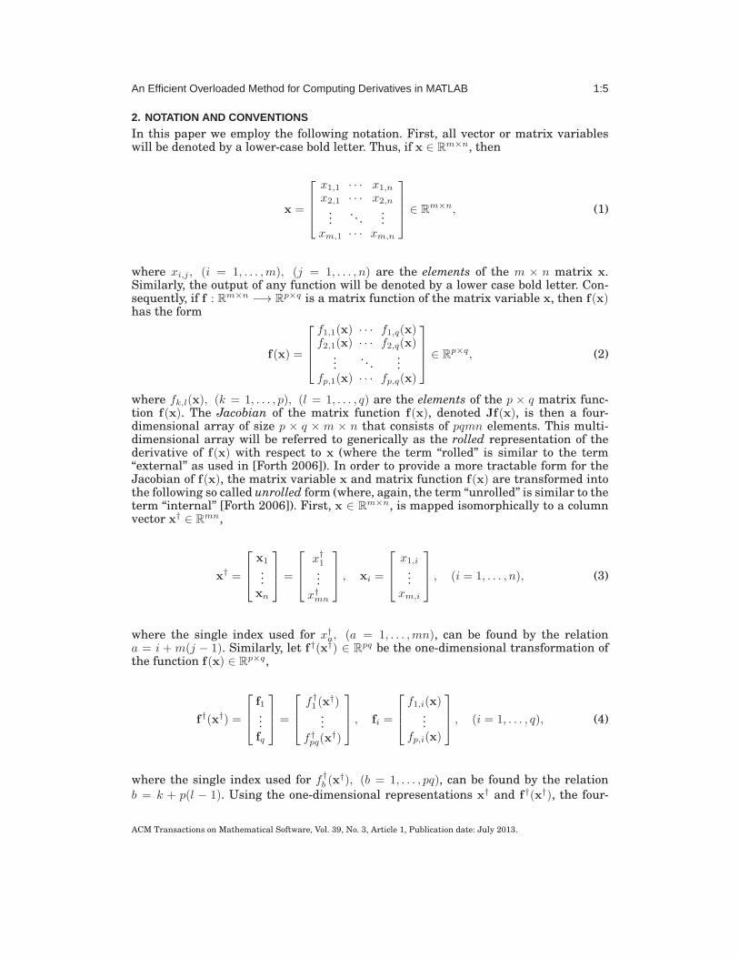
In this paper we employ the following notation. First, all vector or matrix variableswill be denoted by a lower-case bold letter. Thus, if x ∈ R
m×n, then
x =
x1,1 · · · x1,n
x2,1 · · · x2,n
.... . .
...xm,1 · · · xm,n
∈ Rm×n, (1)
where xi,j , (i = 1, . . . ,m), (j = 1, . . . , n) are the elements of the m × n matrix x.Similarly, the output of any function will be denoted by a lower case bold letter. Con-sequently, if f : Rm×n −→ R
p×q is a matrix function of the matrix variable x, then f(x)has the form
f(x) =
f1,1(x) · · · f1,q(x)f2,1(x) · · · f2,q(x)
.... . .
...fp,1(x) · · · fp,q(x)
∈ Rp×q, (2)
where fk,l(x), (k = 1, . . . , p), (l = 1, . . . , q) are the elements of the p × q matrix func-tion f(x). The Jacobian of the matrix function f(x), denoted Jf(x), is then a four-dimensional array of size p × q × m × n that consists of pqmn elements. This multi-dimensional array will be referred to generically as the rolled representation of thederivative of f(x) with respect to x (where the term “rolled” is similar to the term“external” as used in [Forth 2006]). In order to provide a more tractable form for theJacobian of f(x), the matrix variable x and matrix function f(x) are transformed intothe following so called unrolled form (where, again, the term “unrolled” is similar to theterm “internal” [Forth 2006]). First, x ∈ R
m×n, is mapped isomorphically to a columnvector x† ∈ R
mn,
x† =
x1
...xn
=
x†1...
x†mn
, xi =
x1,i
...xm,i
, (i = 1, . . . , n), (3)
where the single index used for x†a, (a = 1, . . . ,mn), can be found by the relation
a = i +m(j − 1). Similarly, let f†(x†) ∈ Rpq be the one-dimensional transformation of
the function f(x) ∈ Rp×q,
f†(x†) =
f1...fq
=
f†1 (x
†)...
f†pq(x
†)
, fi =
f1,i(x)...
fp,i(x)
, (i = 1, . . . , q), (4)
where the single index used for f†b (x
†), (b = 1, . . . , pq), can be found by the relationb = k + p(l − 1). Using the one-dimensional representations x† and f†(x†), the four-
ACM Transactions on Mathematical Software, Vol. 39, No. 3, Article 1, Publication date: July 2013.

1:6 M. A. Patterson, M. Weinstein, and A. V. Rao
dimensional Jacobian, Jf(x) can be represented in two-dimensional form as
Jf†(x†) =
∂f†1
∂x†1
· · ·∂f†
1
∂x†mn
∂f†2
∂x†1
· · ·∂f†
2
∂x†mn
.... . .
...∂f†
pq
∂x†1
· · ·∂f†
pq
∂x†mn
∈ Rpq×mn. (5)
Equation (5) provides what is known as the internal [Forth 2006] two-dimensionalrepresentation of the derivative. It is noted that Jf†(x†) ∈ R
pq×mn in Eq. (5) containsthe same information as the four-dimensional array Jf(x) ∈ R
p×q×m×n. Once a Jaco-bian of a function has been determined in the aforementioned manner, higher-orderderivatives can be computed by repeating the process on Jf†(x†) [Padulo et al. 2008].As an example, starting with x† and Jf†(x†), the Jacobian of Jf†, denoted J2f†(x†),can be computed by transforming Jf† to a one-dimensional array in the manner givenin Eq. (4) and computing J2f†(x†) in a form similar to that given in Eq. (5). The re-sulting matrix J2f†(x†) would then be of size pqmn ×mn. Thus, when starting from amatrix function of a matrix, any order derivative is represented as a two-dimensionalarray. With regard to implementation on a computer, it is much more efficient to iso-morphically map all variables and functions from higher-dimensional quantities toone-dimensional quantities because it provides a more systematic way to referenceand store the derivatives. Finally, it is noted that the method described in this paperutilizes MATLAB object-oriented programming with operator overloading. In order torefer to a MATLAB object that corresponds to a multi-dimensional array y, we use acorresponding calligraphic character, Y. In other words, if y is a vector or matrix, thenY is a MATLAB object that corresponds to y.
3. FORWARD MODE AUTOMATIC DIFFERENTIATION
Using the conventions developed in Section 2, consider a function y = f(x) wheref : Rm×n −→ R
p×q. Assume that f(x) can be reduced to a sequence of elementary func-tion operations (e.g., polynomials, exponential functions, trigonometric functions). Fur-thermore, suppose that a computer implementation of the f(x) has been written in theMATLAB programming language. The goal is to automatically determine Jf(x), thatis, the goal is to determine the derivative of each output function fij , (i = 1, . . . , p), (j =1 . . . , q) with respect to each input element xkl, (k = 1, . . . ,m), (l = 1, . . . , n). Moreover,it is desired to obtain a new MATLAB code that computes these derivatives for futureuse. The method of this paper uses an object-oriented approach that implements for-ward mode automatic differentiation in such a way that each operation in a functionis differentiated in terms of the results of previous operations, and the result of eachoperation is printed to a file. In forward mode differentiation, the chain rule is usedrepeatedly until the step in the chain is encountered where the derivative of the out-ermost function with respect to the input is obtained. In the case of a scalar functiony = f(g(x)), the derivative ∂f/∂x is obtained via the chain rule as
∂f
∂x=
∂f
∂g
∂g
∂x. (6)
Finally, as part of the method developed in this paper, only the nonzero elements of theJacobian are stored, reducing memory requirements and taking advantage of Jacobiansparsity [Forth et al. 2004].
ACM Transactions on Mathematical Software, Vol. 39, No. 3, Article 1, Publication date: July 2013.

An Efficient Overloaded Method for Computing Derivatives in MATLAB 1:7
4. MAJOR COMPONENTS OF METHOD
In this section we describe many of the major components of the method developed inthis paper. Consider again a function of the form y = f(x) where f : Rm×n −→ R
p×q.Next, suppose that a MATLAB class called CADA has been developed, where anyCADA instance, X , corresponds to a two-dimensional real mathematical variablex ∈ R
n×m. Furthermore, assume that overloaded versions of all standard unary math-ematical functions (e.g., polynomial, trigonometric, exponential, etc.), binary mathe-matical functions (e.g., plus, minus, times, etc.) and organizational functions (e.g., re-shape, transpose, matrix, replication, and tiling, etc.) have been written specifically tooperate on CADA objects.
Assume now the user has written a MATLAB code that implements a function y =f(x), where f : Rm×n −→ R
p×q. Assume further that this code can be decomposed into asequence of the aforementioned available overloaded mathematical and organizationalfunctions. CADA is designed to write a new MATLAB code that can compute the an-alytic derivative, ∂fij/∂xkl, (i = 1, . . . , p), (j = 1, . . . , q), (k = 1, . . . ,m), (l = 1, . . . , n),of each function output with respect to each input. Using an object-oriented approach,this new function is obtained by evaluating the function on the input CADA instanceX . When any overloaded function operates on a CADA object, symbolic representa-tions of the result of the overloaded function and the derivative are printed to a filein terms of the input CADA object properties. The output of the overloaded functionis itself another CADA object with the function and derivative properties redefinedto represent the result of the overloaded function. The evaluation of any function isperformed in the usual mathematical manner and derivatives are computed using thewell known rules of differential calculus for each overloaded function. When evalu-ating the resulting derivative code, the output derivative is obtained by applying therules of differential calculus (e.g., sum, product, quotient, and chain rules) until allrules have been completely applied. In the sections that follow, the major componentsof CADA are described along with capabilities that maintain functionality with gen-eral MATLAB code and the ability to generate gradient, Jacobian, and Hessian filesfor use in other applications.
4.1. The CADA Environment
The method of this paper requires that an environment within MATLAB be createdto achieve the goal of generating efficient derivative code. The CADA environmentconsist of three key components, a temporary file to which the derivative code willbe written, a global variable that contains information that is required for each stepin the function evaluation process and the overloaded CADA objects that are beingevaluated. All global information is stored in a global structure named GLOBALCADA.The structure GLOBALCADA has the following fields:
(i) OPERATIONCOUNT: a positive integer that represents the current overloadedoperation count. Each time an overloaded CADA operation is evaluated, thisvalue is incremented by unity. The value of OPERATIONCOUNT is used to cre-ate a unique handle for the resulting CADA object for each overloaded operation.
(ii) LINECOUNT: a positive integer that represents the current number of func-tion lines in the CADA temporary file. Whenever a line of code is written to thetemporary file, the value of LINECOUNT is incremented by unity. The counterLINECOUNT is used to keep track of the location in the temporary file wherelines of code are being written.
(iii) FUNCTIONLOCATION: an N × 2 MATLAB array, where N is the numberof overloaded operations that have been evaluated. Elements (i, 1) and (i, 2) ofFUNCTIONLOCATION contains the starting and ending lines in the temporar-
ACM Transactions on Mathematical Software, Vol. 39, No. 3, Article 1, Publication date: July 2013.

1:8 M. A. Patterson, M. Weinstein, and A. V. Rao
ily file that correspond to the ith overloaded operation that has been executed.The information in FUNCTIONLOCATION is used during the post-processingon the temporary file in order to determine when a function handle can be re-used(see Section 4.8)
(iv) NUMBERVARIABLES: a positive integer that represents the number of CADAinstances in the current environment. The property NUMBERVARIABLES isdefined when the CADA environment is instantiated and never changes during aCADA session.
(v) VARIABLE: a MATLAB cell array of size NUMBERVARIABLES × 3. The{i, 1}, (i = 1, . . . ,NUMBERVARIABLES) element in VARIABLE con-tains the string name of the ith CADA instance, while the {i, 2}, (i =1, . . . ,NUMBERVARIABLES) element in VARIABLE contains a 1×2 numericarray that represents the size of the ith CADA instance. The cell array element{i, 3}, (i = 1, . . . ,NUMBERVARIABLES) contains either unity or zero, wherea unity indicates that the derivatives with respect to the ith CADA instance arebeing calculated, while a zero indicates that the derivatives with respect to theith CADA instance are not being calculated. The property VARIABLE is definedwhen the CADA environment is instantiated and never changes during a CADAsession.
(vi) FID: An integer that identifies the temporary file to which the derivative codewill be written during a CADA session. The property FID is defined when theCADA environment is instantiated and never changes during a CADA session.
4.2. CADA Class and CADA Object Properties
As mentioned previously, the method of this paper is developed via a new overloadedMATLAB object class called CADA. Every CADA object has the following properties:
(i) function: a MATLAB cell array of size 1 × 3, where element {1, 1} contains astring representing the current function handle, element {1, 2} contains a 1×2 nu-meric array that represents the row and column size of the current function. Thecell array element {1, 3} contains a integer that represents the current functioncount. If the CADA object is representing a fixed numerical array then element{1, 1} contains the numeric array.
(ii) derivative: an NUMBERVARIABLES × 2 MATLAB cell array, whereNUMBERVARIABLES is the number of CADA instances in the current CADAenvironment. The cell array element {i, 1}, (i = 1, . . . ,NUMBERVARIABLES),of the derivative cell array contains a string representing the current derivativehandle with respect to the ith CADA instance. The cell array element {i, 2}, (i =1, . . . ,NUMBERVARIABLES), contains a numeric array of size nz×2, where nz
is the number of nonzero derivatives. The indices in this numeric array containthe locations of the nonzero derivatives. More specifically, the first and secondelements in each row of this numeric array contain the function element andvariable element indices, respectively. If the CADA object is representing a fixednumerical array then all cells are empty.
Any CADA object that represents a fixed numeric array must result from overloadedoperations whose output is numeric. Examples of such operations include size, ones,and zeros. The derivatives of such operations are zero. Such CADA objects are referredto as CADA numeric objects.
ACM Transactions on Mathematical Software, Vol. 39, No. 3, Article 1, Publication date: July 2013.
An Efficient Overloaded Method for Computing Derivatives in MATLAB 1:9
4.3. CADA Differentiation Method
The method used in CADA to differentiate a function by evaluating the function onoverloaded CADA objects relies upon the interaction between the different CADA en-vironment properties. When any mathematical operation is evaluated on a CADA ob-ject, the lines of code that represent the mathematical operation and the derivativeof the mathematical operation are printed to a temporary file. As an example of howan overloaded operation is written to the temporary file, consider a mathematical op-eration z = f(x) and assume that this mathematical operation is applied to a CADAobject X , resulting in an output CADA object Z (that is, Z = f(X )). Fig. 1 shows theoperational flow that produces the derivative code for the operation Z = f(X ), where itis seen that information from both the object properties of X and the GLOBALCADAproperties are required to compute the derivative of the operation Z = f(X ). While theobject properties of X contain information from previous overloaded evaluations up tothat point in the overall function, the GLOBALCADA information is needed to definethe function and derivative handles of the output Z. First, a check is performed to de-termine if the input X is a CADA numeric object. In this case the function property ofZ is calculated directly and no code is written to the temporary file. If X is not a CADAnumeric object, new function and derivative handles are defined for Z and the codethat represents z = f(x) and the derivative of z = f(x) are printed to the temporaryfile. In this second case, only the code that corresponds to the nonzero derivatives of theoperation with respect to each CADA instance is written to the temporary file. Becauseonly the nonzero derivatives are written to the temporary file, the method produces asparse representation of the derivative of the function. The details on how the CADAmethod provides a sparse representation of the derivative is given below.
In order to ensure that a sparse representation of the derivative is written to thetemporary file, it is necessary that the appropriate elements of the function propertyof X are properly referenced such that the code resulting from the application of thecalculus chain rule is applied to only the elements in the array whose derivatives arenot zero. The GLOBALCADA properties are also updated during an overloaded opera-tion in the following manner. For every line of code that is written to the temporary fileduring an overloaded operation, the property LINECOUNT is increased by unity. Thelocations of the first and last lines of code that represent the function z = f(x) and thecorresponding derivative are added to the FUNCTIONLOCATION property. Further-more, the location of the last line of code in terms of the function handle representingX is updated. It is noted that the subroutine cadaindprint is used to efficiently printthe derivative indices to the temporary file.
4.4. CADA Setup and Environment Instantiation
The CADA global environment and all CADA instances that are used in generatingderivative code are instantiated using the function cadasetup. The cadasetup func-tion performs the following operations: (1) instantiates the global structure GLOB-ALCADA; (2) defines the initial property values for GLOBALCADA; (3) creates andopens a temporary file named “cada.$#$#[email protected]” to which the deriva-tive code will be written; (4) and creates the initial CADA instances that will be usedduring the CADA session. For each initial CADA instance that is desired, cadasetuprequires the following four inputs: a string containing the name of the CADA instance(where each instance must have a unique name and the name cannot be a MATLABreserved word); two integers that, respectively, define the row and column size of theCADA instance; and an integer flag that indicates whether or not CADA should com-pute derivatives with respect to the particular CADA instance. If the derivative optionflag corresponding to a CADA instance is unity, then derivatives with respect to the
ACM Transactions on Mathematical Software, Vol. 39, No. 3, Article 1, Publication date: July 2013.

1:10 M. A. Patterson, M. Weinstein, and A. V. Rao
If
X.function{1}
is Numeric
Input CADA
Object X
Z.function{1} = f(X.function{1})
Z.function{2} = New Function Size
Z.derivative = empty
TrueFalseFUNhandle = (’cadaf’, OPERATIONCOUNT,’f’)
LINECOUNT = LINECOUNT + 1
Z.function{1} = FUNhandle
Z.function{2} = New Function Size
Z.function{3} = OPERATIONCOUNT
FUNCTIONLOCATION(Z.function{3},1) = LINECOUNT
If
X.derivative{Vcount,1}
is Empty
if
Vcount <= NumVar
Print Code to File FID
Using cadaindprint Subroutine:
cadatf1 = X.function{1}(index)
Where
index = X.derivative{Vcount,2}(:,1)
Print Code to File FID
DERhandle = df(cadatf1).*X.derivative{Vcount,1}
Z.derivative{Vcount,1} = DERhandle
Z.derivative{Vcount,2} = Non-Zero Derivative Index
LINECOUNT = LINECOUNT + 2
FUNCTIONLOCATION(X.function{3},2) = LINECOUNT
FUNCTIONLOCATION(Z.function{3},2) = LINECOUNT
OPERATIONCOUNT = OPERATIONCOUNT + 1
Vcount = Vcount + 1
Vcount = 1
NumVar = NUMBERVARIABLES
True
False
False
True
Print Code to File FID
FUNhandle = f(X.function{1})
DERhandle =
(’dcadaf’, OPERATIONCOUNT,’fd’,VARIABLE{Vcount,1})
Output CADA
Object Z
Fig. 1: Flowchart Describing How an Overloaded Operation Z = f(X ) Produces Deriva-tive Code.
CADA instance are calculated. On the other hand, if the derivative option flag corre-sponding to a CADA instance is zero, derivatives with respect to the CADA instanceare not calculated. The call to the function cadasetup is shown in Fig. 2.
Example of cadasetup Usage. Consider instantiating a CADA session with the threeCADA instances X , Y, and Z, where X , Y, and Z represent, respectively, the variablesx ∈ R
3×1, y ∈ R3×1, and z ∈ R. Furthermore, suppose that it is desired to obtain
derivatives with respect to X and Y, but it is not desired to compute derivatives withrespect to z. Then a MATLAB code that instantiates the CADA session is given asfollows:
[x y z] = cadasetup(’x’,3,1,1,’y’,3,1,1,’z’,1,1,0);
ACM Transactions on Mathematical Software, Vol. 39, No. 3, Article 1, Publication date: July 2013.

An Efficient Overloaded Method for Computing Derivatives in MATLAB 1:11
[v1, v2, ... , vN] = cadasetup(’v1’, v1rows, v1cols, v1�ag, ’v2’, v2rows, v2cols, v2�ag, ... ,’vN’, vNrows, vNcols, vN�ag)
Inputs For CADA
Variable 1
{Inputs For CADA
Variable NUMBERVARIABLES
Inputs For CADA
Variable 2
Variable Name
Variable Row size Variable Column size
Variable Derivative Option
CADA Variable 1
CADA Variable 2
CADA Variable NUMBERVARIABLES
{{Fig. 2: Input/Output Scheme of the CADA Environment Constructor Function.
The properties of GLOBALCADA after instantiation of the CADA environment aregiven as
GLOBALCADA =
OPERATIONCOUNT: 1
LINECOUNT: 0
FUNCTIONLOCATION: [0 0]
NUMBERVARIABLES: 3
VARIABLE: {3x3 cell}
FID: 3
More details of the VARIABLE property of GLOBALCADA are given as
GLOBALCADA.VARIABLE =
’x’ [3 1] [1]
’y’ [3 1] [1]
’z’ [1 1] [0]
It is noted that the GLOBALCADA properties NUMBERVARIABLES, VARIABLE,and FID never change from the instantiated values during the CADA session. Fur-thermore, the object properties of the CADA instance will be shown in detail, the objectproperties of X , Y, and Z are given, respectively, as
x.function =
’x’ [3 1] []
x.derivative =
’cadadxdx’ [3x2 double]
[] []
[] []
x.derivative{1,2} =
1 1
2 2
3 3
y.function =
’y’ [3 1] []
y.derivative =
[] []
’cadadydy’ [3x2 double]
[] []
y.derivative{2,2} =
1 1
2 2
ACM Transactions on Mathematical Software, Vol. 39, No. 3, Article 1, Publication date: July 2013.
1:12 M. A. Patterson, M. Weinstein, and A. V. Rao
3 3
z.function =
’z’ [1 1] []
z.derivative =
[] []
[] []
[] []
Because in this example it was not desired to compute derivatives with respect to Z,the derivative property of Z is instantiated as empty (thus implying that derivativeswith respect to Z will not be computed). For ease of use, an overloaded display func-tion has been implemented for CADA objects, the display shows pertinent informationfrom the CADA object properties in a compact manner. From this point forward in thepaper, all CADA object details will be shown using the overloaded display function.Details of the CADA instances X , Y, and Z are given as follows:
>> x
Current CADA handle:
’x’ size: 3 x 1
Current CADA derivative handles with respect to each variable:
’cadadxdx’ has 3 nonzero derivatives with respect to ’x’
>> y
Current CADA handle:
’y’ size: 3 x 1
Current CADA derivative handles with respect to each variable:
’cadadydy’ has 3 nonzero derivatives with respect to ’y’
>> z
Current CADA handle:
’z’ size: 1 x 1
Because X , Y, and Z represent CADA instances, the indices of the nonzero derivativelocations correspond to those of the identity matrix. In other words, the derivative ofany of these CADA instances with respect to itself is the identity function. Again, itis re-emphasized that these indices correspond to the locations of only the nonzeroderivatives. Moreover, as the derivative is propagated using the forward mode, at eachstep only the nonzero derivatives and their locations are computed. Consequently, thederivative is represented sparsely at each step in the evaluation of the function on theCADA object.
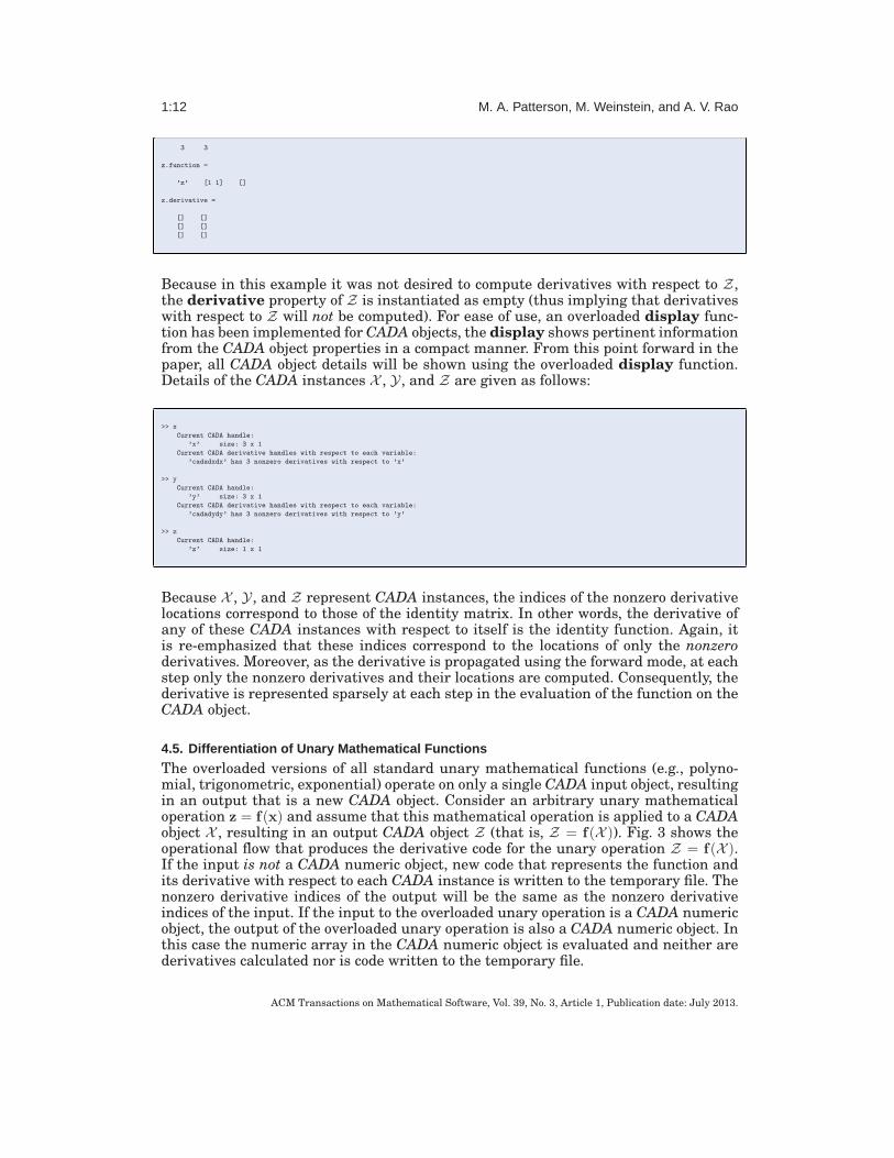
4.5. Differentiation of Unary Mathematical Functions
The overloaded versions of all standard unary mathematical functions (e.g., polyno-mial, trigonometric, exponential) operate on only a single CADA input object, resultingin an output that is a new CADA object. Consider an arbitrary unary mathematicaloperation z = f(x) and assume that this mathematical operation is applied to a CADAobject X , resulting in an output CADA object Z (that is, Z = f(X )). Fig. 3 shows theoperational flow that produces the derivative code for the unary operation Z = f(X ).If the input is not a CADA numeric object, new code that represents the function andits derivative with respect to each CADA instance is written to the temporary file. Thenonzero derivative indices of the output will be the same as the nonzero derivativeindices of the input. If the input to the overloaded unary operation is a CADA numericobject, the output of the overloaded unary operation is also a CADA numeric object. Inthis case the numeric array in the CADA numeric object is evaluated and neither arederivatives calculated nor is code written to the temporary file.
ACM Transactions on Mathematical Software, Vol. 39, No. 3, Article 1, Publication date: July 2013.

An Efficient Overloaded Method for Computing Derivatives in MATLAB 1:13
True
False
Input CADA
Object X
Output CADA
Object Z
If
X is CADA Numeric
Z.function{1} = f(X.function{1})
Z.function{2} = X.function{2}
Z.derivative = empty
De!ne New Function Handle.
Print Code to File FID to Evaluate the Function.
De!ne the function Property of Output Z.
Update GLOBALCADA Properties.
For Each CADA Variable
De!ne New Derivative Handle.
Print Code to File FID to Evaluate the
Nonzero Derivatives With Respect to the
Current Constructor Variable in X.
De!ne the derivative Property of Output Z.
Update GLOBALCADA Properties.
Fig. 3: Flowchart Describing How an Overloaded Unary Operation Z = f(X ) ProducesDerivative Code.
Example of Unary Mathematical Function. Consider evaluating the unary mathe-matical function a = sin(x) on the CADA object X from the example in Section 4.4. TheMATLAB code to evaluate A = sin(X ) is as follows.
>> a = sin(x)
Current CADA handle:
’cadaf1f’ size: 3 x 1
Current CADA derivative handles with respect to each variable:
’dcadaf1fdx’ has 3 nonzero derivatives with respect to ’x’
The temporary file then contains the code that calculates both the function a = sin(x)and the nonzero derivatives of a = sin(x) as seen in the following lines of code:
cadaf1f = sin(x);
cadatf1 = x(1:3);
dcadaf1fdx = cos(cadatf1(:)).*cadadxdx;
In the above code segment the quantity ’cadadxdx’ is the derivative of the CADA in-stance X and will be defined in a post-processing step that manipulates the temporaryfile into a executable MATLAB function (see Section 4.8 below). In order to ensurethat only the nonzero derivatives are computed, the proper elements of x need to bereferenced using the nonzero derivative indices in X in the line ’cadatf1 = x(1:3)’. Thechain rule for the nonzero elements of a is applied using array multiplication in theline ’dcadaf1fdx = cos(cadatf1(:)).*cadadxdx;’. The properties of GLOBALCADA afterthe evaluation of A = sin(X ) are as follows:
GLOBALCADA =
OPERATIONCOUNT: 2
LINECOUNT: 3
FUNCTIONLOCATION: [1 3]
NUMBERVARIABLES: 3
ACM Transactions on Mathematical Software, Vol. 39, No. 3, Article 1, Publication date: July 2013.

1:14 M. A. Patterson, M. Weinstein, and A. V. Rao
VARIABLE: {3x3 cell}
FID: 3
In the above code segment, the property OPERATIONCOUNT has been increased byone, the property LINECOUNT is equal to the number of lines of code in the tempo-rary file, and the property FUNCTIONLOCATION now shows that the CADA func-tion handle ’cadaf1f ’ is used in lines 1 through 3 of the temporary file.
4.6. Differentiation of Binary Mathematical Functions
The overloaded binary mathematical functions (e.g., plus, minus, times, array multi-plication) have two inputs, where at least one of the inputs must be a CADA object andthe output is a CADA object. Consider a binary mathematical operation z = f(x,y).If x is a CADA object but y is not a CADA object, then the function is evaluated asZ = f(X ,y). Similarly, if y is a CADA object but x is not a CADA object, then thefunction is evaluated as Z = f(x,Y). Finally, if both x and y are CADA objects, thenthe function is evaluated as Z = f(X ,Y). Fig. 4 shows the operational flow that pro-duces the derivative code for the binary operation Z = f(x,y). First, it is necessary todetermine the class of each input. If only one of the inputs is a CADA object, then theoperation follows in a manner similar to that of a unary function. In the case whereboth inputs are CADA objects, it is necessary to determine if any or both inputs areCADA numeric objects. If both inputs are CADA numeric objects, the function is eval-uated on the numeric values of X and Y, resulting in the CADA numeric object Z.Furthermore, as is the case with all CADA numeric objects, no derivatives are calcu-lated and no code is written to the temporary file. If exactly one of the two inputs is aCADA numeric object, the numeric value of the CADA numeric object is found and theoverloaded operation is performed as if only one of the inputs is a CADA object. Lastly,if both CADA objects contain derivatives with respect to the same CADA instance,the binary chain rule (e.g., product rule, quotient rule, etc.) is applied to calculate thenonzero derivatives. The nonzero derivative indices of the output are determined bytaking the union of the nonzero derivative indices of X and Y.
Example of Binary Mathematical Functions. Let b = a ⊗ y represent element-by-element multiplication of a and y. Furthermore, let A be the CADA object from theexample of Section 4.5 and let Y be the CADA object from the example of Section 4.4.The MATLAB code that evaluates B = A⊗ Y is as follows:
>> b = a.*y
Current CADA handle:
’cadaf2f’ size: 3 x 1
Current CADA derivative handles with respect to each variable:
’dcadaf2fdx’ has 3 nonzero derivatives with respect to ’x’
’dcadaf2fdy’ has 3 nonzero derivatives with respect to ’y’
The temporary file now contains the code that calculates the function and the nonzeroderivatives of b = a⊗ y and is given as
cadaf1f = sin(x);
cadatf1 = x(1:3);
dcadaf1fdx = cos(cadatf1(:)).*cadadxdx;
cadaf2f = cadaf1f .* y;
cadatf1 = y(1:3);
dcadaf2fdx = cadatf1(:).*dcadaf1fdx;
cadatf1 = cadaf1f(1:3);
dcadaf2fdy = cadatf1(:).*cadadydy;
ACM Transactions on Mathematical Software, Vol. 39, No. 3, Article 1, Publication date: July 2013.

An Efficient Overloaded Method for Computing Derivatives in MATLAB 1:15
False
False False
False
False
True
True
True
True
True
De ne New Function Handle.
Print Code to File FID to Evaluate the
Function in terms Y.
De ne the function Property of Output Z.
Update GLOBALCADA Properties.
For Each CADA Variable
De ne New Derivative Handle.
Print Code to File FID to Evaluate the
Nonzero Derivatives With Respect to the
Current Constructor Variable inY.
De ne the derivative Property of Output Z.
Update GLOBALCADA Properties.
De ne New Function Handle.
Print Code to File FID to Evaluate the
Function in terms X.
De ne the function Property of Output Z.
Update GLOBALCADA Properties.
For Each CADA Variable
De ne New Derivative Handle.
Print Code to File FID to Evaluate the
Nonzero Derivatives With Respect to the
Current Constructor Variable in X.
De ne the derivative Property of Output Z.
Update GLOBALCADA Properties.
De ne New Function Handle.
Print Code to File FID to Evaluate the
Function in terms X and Y.
De ne the function Property of Output Z.
Update GLOBALCADA Properties.
For Each CADA Variable
De ne New Derivative Handle.
Print Code to File FID to Evaluate the
Nonzero Derivatives With Respect to the
Current Constructor Variable in X and Y.
De ne the derivative Property of Output Z.
Update GLOBALCADA Properties.
If
Y is CADA Numeric
y = Y.function{1}
If
Y is CADA Numeric
If
Y is CADA Numeric
If
X is CADA Numeric
x = X.function{1}
If
X is CADA Numeric
If
x is a CADA
Object
If
x and y are CADA
Objects
True
True
y = Y.function{1}
y = Y.function{1}x = X.function{1}
False
False
Output CADA
Object Z
Input
x, y
Z.function{1} = f(x,y)
Z.function{2} = Size of f(x,y)
Z.derivative = empty
Fig. 4: Flowchart Describing How an Overloaded binary Operation Z = f(X ) ProducesDerivative Code.
In the aforementioned code segment the quantity ’cadadydy’ is the Y with respectto the CADA instance and will be defined in a post-processing step that transformsthe temporary file into a executable MATLAB function (see Section 4.8 below). Whencomputing the nonzero derivatives of b with respect to x, the proper elements of y arereferenced using the nonzero derivative indices in A as shown in the line ’cadatf1 =y(1:3)’. The chain rule to obtain the nonzero derivatives with respect to x is applied viaarray multiplication in the line ’dcadaf2fdx = cadatf1(:).*dcadaf1fdx’. When computingthe nonzero derivatives of b with respect to y, the proper elements of A are referencedusing the nonzero derivative index in Y on line ’cadatf1 = cadaf1f(1:3)’. The chain ruleto obtain the nonzero derivatives respect to y is then applied via array multiplication in
ACM Transactions on Mathematical Software, Vol. 39, No. 3, Article 1, Publication date: July 2013.

1:16 M. A. Patterson, M. Weinstein, and A. V. Rao
the line ’cadatf1 = cadaf1f(1:3)’. The properties of GLOBALCADA after the evaluationof B = A⊗ Y are as follows:
GLOBALCADA =
OPERATIONCOUNT: 3
LINECOUNT: 8
FUNCTIONLOCATION: [2x2 double]
NUMBERVARIABLES: 3
VARIABLE: {3x3 cell}
FID: 3
In the aforementioned code segment, the property OPERATIONCOUNT has beenincreased by one, and the property LINECOUNT is equal to the number of lines ofcode in the temporary file. The contents of the FUNCTIONLOCATION is shown as
GLOBALCADA.FUNCTIONLOCATION =
1 8
4 8
The quantity FUNCTIONLOCATION now shows that the CADA function handle’cadaf1f ’ is used in lines 1 through 8, and the CADA function handle ’cadaf2f ’ is usedin lines 4 through 8 of the temporary file.
4.7. Array Referencing, Assignment, and Concatenation on CADA Objects
The operations of referencing, assignment, and concatenation have the unifying fea-ture that none of them performs any mathematical calculations on array elements.Instead, these operations only alter the locations of these elements in an array. Ref-erencing the elements of an array creates an output that consist of a subset of theoriginal array. Similarly, assigning elements into an array results in a new array thatincludes elements in the assigned locations. Finally, concatenation merges multiplearrays into a new array. The overloaded referencing, assignment, and concatenationoperations for CADA generate code that performs in the same standard way as thestandard non-overloaded versions of these functions. The overloaded CADA versionsof these operations, however, keeps track of the derivatives of the elements that havebeen referenced, assigned, or concatenated, thus, preserving the nonzero derivativesof every element with respect to the CADA instance.
Example of Concatenation. Consider the operation of vertical concatenation,
c =
[
zb
]
. (7)
In this example the vertical concatenation operation is applied to the CADA object Zfrom the example in Section 4.4 and the CADA object B from the example in Section4.6. The MATLAB code that performs the vertical concatenation given in Eq. (7) on Zand B is given as
>> c = [z; b]
Current CADA handle:
’cadaf3f’ size: 4 x 1
Current CADA derivative handles with respect to each variable:
’dcadaf3fdx’ has 3 nonzero derivatives with respect to ’x’
’dcadaf3fdy’ has 3 nonzero derivatives with respect to ’y’
The result of the aforementioned code segment is that the temporary file contains thecode that performs the vertical concatenation shown in Eq. (7). The nonzero derivatives
ACM Transactions on Mathematical Software, Vol. 39, No. 3, Article 1, Publication date: July 2013.

An Efficient Overloaded Method for Computing Derivatives in MATLAB 1:17
of c with respect to x and y are then found by defining new indices for the nonzeroderivatives of b as follows:
cadaf1f = sin(x);
cadatf1 = x(1:3);
dcadaf1fdx = cos(cadatf1(:)).*cadadxdx;
cadaf2f = cadaf1f .* y;
cadatf1 = y(1:3);
dcadaf2fdx = cadatf1(:).*dcadaf1fdx;
cadatf1 = cadaf1f((1:3));
dcadaf2fdy = cadatf1(:).*cadadydy;
cadaf3f = vertcat(z,cadaf2f);
dcadaf3fdx = zeros(3,cadaunit);
dcadaf3fdx((1:3)) = dcadaf2fdx;
dcadaf3fdy = zeros(3,cadaunit);
dcadaf3fdy((1:3)) = dcadaf2fdy;
The derivative indices corresponding to the nonzero derivatives in C are found in thederivative property of C as
c.derivative{1,1} =
dcadaf3fdx
c.derivative{1,2} =
2 1
3 2
4 3
c.derivative{2,1} =
dcadaf3fdy
c.derivative{2,2} =
2 1
3 2
4 3
It is seen the this last code segment that the derivative indices of C have been alteredbased on the vertically concatenated objects Z and B.
4.8. Post-Processing of Temporary File to Create Derivative Funct ion
Once the desired function evaluations have been completed within the CADA environ-ment, the resulting temporary file is post-processed in order to obtain the derivativefunction file for use with MATLAB. The post-processing of the temporary file is dividedinto the following two parts: (1) reassignment of function and derivative function han-dle names that were created when the temporary file was written and (2) formattingthe nonzero derivative values and their corresponding indices into the desired output.Each of these steps is now described, along with a rationale for why it is important toreassign function handles as alluded to in step (1).
4.8.1. Re-Numbering of Function and Derivative Handles in Final Derivative Code. In the pro-cess of performing this research, we encountered an issue that MATLAB has a limiton the number of variables that can be created in its workspace (we note that Forthet al. [2004] and Tadjouddine et al. [2002] encountered similar issues with regard torunning out of registers). If the number of variables exceeds this limit, MATLAB willterminate a function call with an error stating that this limit has been exceeded. Be-cause the derivative code created by CADA produces a function and derivative handlefor every mathematical operation that is differentiated, it is realistic that this limitmay be encountered. Reducing the number of variables in the workspace also reducesthe amount of memory needed to execute the function, and improves performance.Thus, it is important to reduce the number of unique function handles that exist in thederivative file.
ACM Transactions on Mathematical Software, Vol. 39, No. 3, Article 1, Publication date: July 2013.

1:18 M. A. Patterson, M. Weinstein, and A. V. Rao
The following approach was used to greatly reduce the number of unique functionhandles in the final derivative code. From the FUNCTIONLOCATION property ofthe GLOBALCADA variable, the lines corresponding to the first and last occurrenceof each intermediate function and its derivatives are known. Using this information,a sorting algorithm is used to determine those function and derivative handles thatcan be replaced by previously used handles, where the previously used handles do notoccur later in the derivative file. Then, when the final derivative file is written, the oldfunction number for each intermediate function and derivative is replaced by a previ-ously used function number. If there is no previously used function number available,the number does not change. For example, suppose that n is a particular overloadedoperation and cadafnf and dcadafnfdx are the function handle strings associated withthis overloaded operation. If a function handle number m has been used earlier in thetemporary file and this lower-numbered function handle is no longer needed at thepoint in the file where function handle n appears, then every occurrence of cadafnf anddcadafnfdx can be replaced with cadafmf and dcadafmfdx. Using this approach, thefinal derivative file will contain the fewest number of unique function handles as pos-sible, thus reducing the number of unique variables that are created in the workspacewhen evaluating the derivative file on a numeric input.
4.8.2. Printing File with Nonzero Derivatives and Corresponding Indices. The final derivativefile can be created in one of three ways. First, suppose that the function being differ-entiated is either a scalar function of a vector or a vector function of a vector, that is,y = f(x) where f : Rn −→ R
m. In this case the file that evaluates the the functionand Jacobian of f(x) can be printed using the CADA function cadajacobian. Second,suppose we restrict attention to a scalar function of a vector, that is, y = f(x) wheref : Rn −→ R. In this case a file that outputs the function, gradient, and Hessian can becreated using function cadahessian. In both of these cases the derivative (Jacobianor Hessian) is written as a sparse matrix in MATLAB. If desired, cadajacobian andcadahessian can also produce an additional executable function that outputs only thesparsity pattern of the corresponding Jacobian or Hessian function. The third and finalcase of printing derivatives corresponds to a function that is neither a scalar or vectorfunction of a vector. In this case it is not possible to use either cadajacobian or cada-hessian. Instead, in this more general case a MATLAB function called cadagenderivmust be used. When using the function cadagenderiv, the nonzero derivatives, alongwith their unrolled indices [see Eq. (5)]. When using the function cadagenderiv it isnecessary for the user to have knowledge of the relationship between the indices corre-sponding to the unrolled representation of the derivative and the rolled representation(that is, the indices in the actual multi-dimensional derivative).
Example of Post-Processing. Consider again the example in Section 4.7. Supposethat it is desired to compute the derivatives of c with respect to x and y, where xand y were defined in the example in Section 4.4. These derivatives can be printedto a derivative file by applying the function cadagenderiv to the CADA object C asfollows:
>> cadagenderiv(c,’ExampleDerivative’)
In the process of applying cadagenderiv to the CADA object C, the temporary file hasbeen removed and the derivative file, ’ExampleDerivative.m’, has been created. Thefile ’ExampleDerivative.m” is an executable MATLAB and given as
ACM Transactions on Mathematical Software, Vol. 39, No. 3, Article 1, Publication date: July 2013.

An Efficient Overloaded Method for Computing Derivatives in MATLAB 1:19
function output = ExampleDerivative(input)
x = input.x;
y = input.y;
z = input.z;
cadadxdx = ones(3,1);
cadadydy = ones(3,1);
cadaunit = size(x(1),1);
cadaf1f = sin(x);
cadatf1 = x((1:3));
dcadaf1fdx = cos(cadatf1(:)).*cadadxdx;
cadaf2f = cadaf1f .* y;
cadatf1 = y((1:3));
dcadaf2fdx = cadatf1(:).*dcadaf1fdx;
cadatf1 = cadaf1f((1:3));
dcadaf2fdy = cadatf1(:).*cadadydy;
cadaf3f = vertcat(z,cadaf2f);
dcadaf3fdx = zeros(3,cadaunit);
dcadaf3fdx((1:3)) = dcadaf2fdx;
dcadaf3fdy = zeros(3,cadaunit);
dcadaf3fdy((1:3)) = dcadaf2fdy;
output.f1.value = cadaf3f;
output.f1.dx.value = dcadaf3fdx;
cadadind1 = [2 7 12];
[cadadind1,cadadind2] = ind2sub([4,3],cadadind1);
output.f1.dx.location = [cadadind1’,cadadind2’];
output.f1.dy.value = dcadaf3fdy;
cadadind1 = [2 7 12];
[cadadind1,cadadind2] = ind2sub([4,3],cadadind1);
output.f1.dy.location = [cadadind1’,cadadind2’];
Because the function cadagenderiv is designed for any number of input CADA in-stances and any number of output functions, the input and output of the executablefile are structured in order to better organize the resulting evaluations. In order to seehow the input and output are organized, consider the following numerical values of x,y, and z:
x =
[
123
]
, y =
[
456
]
, z = 7. (8)
The function ExampleDerivative.m is then evaluated using MATLAB on these numer-ical inputs as follows:
>> input.x = [1; 2; 3];
>> input.y = [4; 5; 6];
>> input.z = 7;
>> output = ExampleDerivative(input);
The value of c, the derivatives of c with respect to x and y, and the locations of thederivatives of c with respect to x and y, when evaluated on the numeric inputs givenin Eq. (8), are then given as
output.f1.value =
7.0000
3.3659
4.5465
0.8467
output.f1.dx.value =
2.1612
-2.0807
-5.9400
output.f1.dx.location =
2 1
3 2
4 3
output.f1.dy.value =
ACM Transactions on Mathematical Software, Vol. 39, No. 3, Article 1, Publication date: July 2013.

1:20 M. A. Patterson, M. Weinstein, and A. V. Rao
0.8415
0.9093
0.1411
output.f1.dy.location =
2 1
3 2
4 3
It is noted that only the nonzero derivatives with respect to x and y are computed (thatis, derivatives corresponding to the nonzero locations), and derivatives with respect toz are not calculated because z was declared during the setup to be a variable for whichderivatives were not desired.
5. EXAMPLES
In this section we apply CADA to four examples. The examples provide coverage of thesignificant capabilities of CADA and compare CADA against other leading automaticdifferentiation software. The first example is the classic Speelpenning problem wherethe goal is to demonstrate that CADA avoids expression explosion when computingthe derivative. The analysis of the Speelpenning problem also contains a comparisonof CADA with the MATLAB Symbolic Math Toolbox where it is well known that sym-bolic differentiation does suffer from expression explosion. The second example is theArrowhead function where the goal is to compare the efficiency of CADA against theleading operator overloaded software programs INTLAB [Rump 1999], ADMAT [Cole-man and Verma 1998a; CAYUGA RESEARCH 2009], and MAD [Forth 2006]. The resultsof this second example show that CADA compares favorably with the computationalefficiency of INTLAB and outperforms both ADMAT and MAD. In addition, the secondexample demonstrates the ability of CADA to generate not only sparse code, but alsocode that is vectorized if the original function code is vectorized. The third exampleis the Brown function from the MATLAB optimization toolbox. The goal of the thirdexample is to demonstrate the efficiency with which CADA generates the Hessian ofa scalar function of a vector and to compare the efficiency of CADA against INTLAB,ADMAT, and MAD when evaluating the Hessian. The fourth example is a large sparsenonlinear programming problem (NLP). The objective of the fourth example is to showthe ability of CADA to generate the constraint Jacobian and Lagrangian Hessian of acomplex NLP. Similar to the first three examples, in the fourth example the efficiencyof CADA is compared against INTLAB, ADMAT, and MAD. Finally, it is noted that allcomputations shown in this section were performed using an Apple MacPro 2.26 GHzQuad-Core Intel Xeon computer with 16 GB of RAM running Mac OS-X Snow Leopardversion 10.6.8 and MATLAB R2010b [Mathworks 2010].
Example 1: Speelpenning Problem
Consider the following function [Speelpenning 1980]:
f(x) =
n∏
i=1
xi, x ∈ Rn, f : Rn −→ R. (9)
It is well known that the derivatives of the function in Eq. (9) are prone to expres-sion explosion as n gets large when Eq. (9) is implemented in the form considered inSpeelpenning [1980] (that is, the function is implemented in the form of a loop as op-posed to using the built-in product function in MATLAB). A code that utilizes a loop toevaluate the function in Eq. (9) is shown in Fig. 5. Because Eq. (9) requires the compu-tation of a product of length n, the gradient requires the computation of n− 1 productsbetween the n terms. The goal of this example is to demonstrate the effectiveness with
ACM Transactions on Mathematical Software, Vol. 39, No. 3, Article 1, Publication date: July 2013.

An Efficient Overloaded Method for Computing Derivatives in MATLAB 1:21
which CADA avoids function explosion when writing the file that is capable of comput-ing the gradient of Eq. (9), and the corresponding efficiency with which the resultingderivative code executes on a numeric argument. In this analysis the results obtainedusing CADA are compared against the MATLAB Symbolic Toolbox (see Mathworks[2010]).
function y = speelpenning4sym(x, n)
y = x(1);
for Icount = 2:n;
y = y.*x(Icount);
end
Fig. 5: File Containing MATLAB Implementation of the Function in Eq. (9).
First consider the manner in which the gradient file is written using CADA. Forthe purpose of this first part of this example, let n = 6. The code corresponding to thetemporary file created by CADA prior to post-processing is shown in Fig. 6. Specifically,it is seen in Fig. 6 that eleven individual operations are performed, thus leading to thecreation of eleven function handles (and corresponding derivative function handles)in the temporary derivative file, and that the sequence of operations written to thetemporary derivative file are the same as those that would have been obtained hadthe forward mode been applied on a numeric value of the vector x. Furthermore, acloser examination of Fig. 6 shows that in the early part of the temporary file the firstthree function handles (defined in the lines containing ’cadaf1f ’, ’cadaf2f ’, ’cadaf3f ’,’dcadaf1fdx’, ’dcadaf2fdx’, and ’dcadaf3fdx’) can be re-used after the sixth line withoutcreating a variable conflict. As a result, higher-numbered function handles after thesixth line in the temporary file can be replaced with these lower-numbered functionhandles from before the sixth line. As a result the number of function handles in thefinal derivative file can be reduced significantly when post-processing the derivativefile using the post-processing step as described in Section 4.8. Figure. 7 shows how thepost-processing of the temporary derivative file reduces the number of unique functionhandles in the final file. It is seen in the final derivative file that the first three functionhandles, created in lines one through six in the temporary file, are re-used later in thefile, thus reducing the number of newly created variables in the MATLAB workspacewhen evaluating the derivative file on a numeric input.
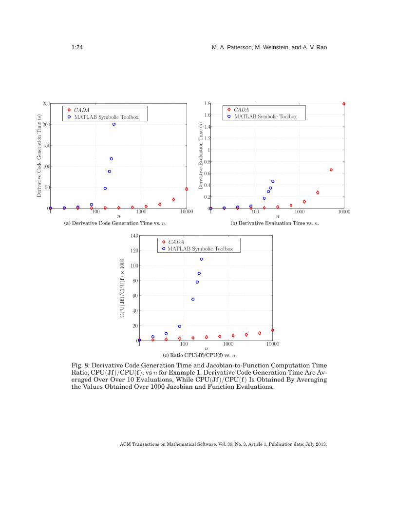
Next, we compare the efficiency with which CADA and the MATLAB Symbolic MathToolbox both to generate and evaluate the derivatives code. Figures 8a–8c show, re-spectively, the derivative code generate time required by CADA and the MATLAB Sym-bolic Math Toolbox, the computation time required to evaluate the resulting derivativefunctions using each generated file on an input vector of all ones, and the gradient-to-function computation time ratio. It is seen that the derivative file is created muchmore quickly using CADA as compared with the MATLAB Symbolic Toolbox, and thistime difference grows quickly as n increases. As an example, for n = 250 the MATLABSymbolic Math Toolbox creates the derivative file in approximately 200 s. On the otherhand, it takes CADA approximately 45 s to create the derivative file for n = 10000.Furthermore, it can be seen in Fig. 8a that the time required to produce the deriva-tive file using the MATLAB Symbolic Toolbox appears to asymptotically approachesa vertical at n ≈ 316. The rapid growth in derivative code generation times for theMATLAB Symbolic Toolbox is a result of expression explosion, where the symbolic ex-pression grows in size and complexity such that the effort required to differentiate theexpression becomes so large that the process becomes intractable. However, the CADA
ACM Transactions on Mathematical Software, Vol. 39, No. 3, Article 1, Publication date: July 2013.

1:22 M. A. Patterson, M. Weinstein, and A. V. Rao
cadaf1f = x(1);
dcadaf1fdx = cadadxdx(1);
cadaf2f = x(2);
dcadaf2fdx = cadadxdx(2);
cadaf3f = cadaf1f .* cadaf2f;
dcadaf3fdx = zeros(2,cadaunit);
cadadind1 = 1;
cadadind2 = 2;
cadatf1 = cadaf1f(1);
cadatf2 = cadaf2f(1);
dcadaf3fdx(cadadind1) = cadatf2(:).*dcadaf1fdx;
dcadaf3fdx(cadadind2) = dcadaf3fdx(cadadind2) + cadatf1(:).*dcadaf2fdx;
cadaf4f = x(3);
dcadaf4fdx = cadadxdx(3);
cadaf5f = cadaf3f .* cadaf4f;
dcadaf5fdx = zeros(3,cadaunit);
cadadind1 = (1:2);
cadadind2 = 3;
cadatf1 = cadaf3f(1);
cadatf2 = cadaf4f(1*ones(2,1));
dcadaf5fdx(cadadind1) = cadatf2(:).*dcadaf3fdx;
dcadaf5fdx(cadadind2) = dcadaf5fdx(cadadind2) + cadatf1(:).*dcadaf4fdx;
cadaf6f = x(4);
dcadaf6fdx = cadadxdx(4);
cadaf7f = cadaf5f .* cadaf6f;
dcadaf7fdx = zeros(4,cadaunit);
cadadind1 = (1:3);
cadadind2 = 4;
cadatf1 = cadaf5f(1);
cadatf2 = cadaf6f(1*ones(3,1));
dcadaf7fdx(cadadind1) = cadatf2(:).*dcadaf5fdx;
dcadaf7fdx(cadadind2) = dcadaf7fdx(cadadind2) + cadatf1(:).*dcadaf6fdx;
cadaf8f = x(5);
dcadaf8fdx = cadadxdx(5);
cadaf9f = cadaf7f .* cadaf8f;
dcadaf9fdx = zeros(5,cadaunit);
cadadind1 = (1:4);
cadadind2 = 5;
cadatf1 = cadaf7f(1);
cadatf2 = cadaf8f(1*ones(4,1));
dcadaf9fdx(cadadind1) = cadatf2(:).*dcadaf7fdx;
dcadaf9fdx(cadadind2) = dcadaf9fdx(cadadind2) + cadatf1(:).*dcadaf8fdx;
cadaf10f = x(6);
dcadaf10fdx = cadadxdx(6);
cadaf11f = cadaf9f .* cadaf10f;
dcadaf11fdx = zeros(6,cadaunit);
cadadind1 = (1:5);
cadadind2 = 6;
cadatf1 = cadaf9f(1);
cadatf2 = cadaf10f(1*ones(5,1));
dcadaf11fdx(cadadind1) = cadatf2(:).*dcadaf9fdx;
dcadaf11fdx(cadadind2) = dcadaf11fdx(cadadind2) + cadatf1(:).*dcadaf10fdx;
Fig. 6: Temporary Derivative File Created by CADA for Speelpenning Problem withn = 6.
derivative code generation times grow at a significantly slower rate as a function ofn. Next, examining Fig. 8b it is seen that the time required to compute the derivativeusing the code generated by CADA is reduced when compared to the code generatedby the MATLAB Symbolic Toolbox. Moreover, examining Fig. 8c, it is seen that theratio CPU(Jf)/CPU(f) grows rapidly using the MATLAB symbolic toolbox because ofexpression explosion, while CPU(Jf)/CPU(f) using CADA grows at a slightly fasterthan logarithmic rate because CADA does not suffer from the expression explosionseen in the MATLAB symbolic toolbox.
ACM Transactions on Mathematical Software, Vol. 39, No. 3, Article 1, Publication date: July 2013.

An Efficient Overloaded Method for Computing Derivatives in MATLAB 1:23
function [Jac,Fun] = speelpenning_Jac(x)
cadadxdx = ones(6,1);
cadaunit = size(x(1),1);
cadaf1f = x(1);
dcadaf1fdx = cadadxdx(1);
cadaf2f = x(2);
dcadaf2fdx = cadadxdx(2);
cadaf3f = cadaf1f .* cadaf2f;
dcadaf3fdx = zeros(2,cadaunit);
cadadind1 = 1;
cadadind2 = 2;
cadatf1 = cadaf1f(1);
cadatf2 = cadaf2f(1);
dcadaf3fdx(cadadind1) = cadatf2(:).*dcadaf1fdx;
dcadaf3fdx(cadadind2) = dcadaf3fdx(cadadind2) + cadatf1(:).*dcadaf2fdx;
cadaf1f = x(3);
dcadaf1fdx = cadadxdx(3);
cadaf2f = cadaf3f .* cadaf1f;
dcadaf2fdx = zeros(3,cadaunit);
cadadind1 = (1:2);
cadadind2 = 3;
cadatf1 = cadaf3f(1);
cadatf2 = cadaf1f(1*ones(2,1));
dcadaf2fdx(cadadind1) = cadatf2(:).*dcadaf3fdx;
dcadaf2fdx(cadadind2) = dcadaf2fdx(cadadind2) + cadatf1(:).*dcadaf1fdx;
cadaf3f = x(4);
dcadaf3fdx = cadadxdx(4);
cadaf1f = cadaf2f .* cadaf3f;
dcadaf1fdx = zeros(4,cadaunit);
cadadind1 = (1:3);
cadadind2 = 4;
cadatf1 = cadaf2f(1);
cadatf2 = cadaf3f(1*ones(3,1));
dcadaf1fdx(cadadind1) = cadatf2(:).*dcadaf2fdx;
dcadaf1fdx(cadadind2) = dcadaf1fdx(cadadind2) + cadatf1(:).*dcadaf3fdx;
cadaf2f = x(5);
dcadaf2fdx = cadadxdx(5);
cadaf3f = cadaf1f .* cadaf2f;
dcadaf3fdx = zeros(5,cadaunit);
cadadind1 = (1:4);
cadadind2 = 5;
cadatf1 = cadaf1f(1);
cadatf2 = cadaf2f(1*ones(4,1));
dcadaf3fdx(cadadind1) = cadatf2(:).*dcadaf1fdx;
dcadaf3fdx(cadadind2) = dcadaf3fdx(cadadind2) + cadatf1(:).*dcadaf2fdx;
cadaf1f = x(6);
dcadaf1fdx = cadadxdx(6);
cadaf11f = cadaf3f .* cadaf1f;
dcadaf11fdx = zeros(6,cadaunit);
cadadind1 = (1:5);
cadadind2 = 6;
cadatf1 = cadaf3f(1);
cadatf2 = cadaf1f(1*ones(5,1));
dcadaf11fdx(cadadind1) = cadatf2(:).*dcadaf3fdx;
dcadaf11fdx(cadadind2) = dcadaf11fdx(cadadind2) + cadatf1(:).*dcadaf1fdx;
cadadind1 = (1:6);
[cadadind1,cadadind2] = ind2sub([1,6],cadadind1);
Jac = sparse(cadadind1,cadadind2,dcadaf11fdx,1,6);
Fun = cadaf11f;
Fig. 7: Final Derivative File Created by CADA for Speelpenning Problem with n = 6.
ACM Transactions on Mathematical Software, Vol. 39, No. 3, Article 1, Publication date: July 2013.
1:24 M. A. Patterson, M. Weinstein, and A. V. Rao
DerivativeCodeGenerationTim
e(s)
n
MATLAB Symbolic Toolbox
50
100
150
200
250CADA
10
100 1000 10000
(a) Derivative Code Generation Time vs. n.
DerivativeEvaluationTim
e(s)
n
MATLAB Symbolic Toolbox
CADA
0.2
0.4
0.6
0.8
1
1
1.2
1.4
1.6
1.8
0100 1000 10000
(b) Derivative Evaluation Time vs. n.
CPU(Jf)/CPU(f)×1000
n
MATLAB Symbolic ToolboxCADA
10
100 1000 10000
20
40
60
80
100
120
140
(c) Ratio CPU(Jf)/CPU(f) vs. n.
Fig. 8: Derivative Code Generation Time and Jacobian-to-Function Computation TimeRatio, CPU(Jf)/CPU(f), vs n for Example 1. Derivative Code Generation Time Are Av-eraged Over Over 10 Evaluations, While CPU(Jf)/CPU(f) Is Obtained By Averagingthe Values Obtained Over 1000 Jacobian and Function Evaluations.
ACM Transactions on Mathematical Software, Vol. 39, No. 3, Article 1, Publication date: July 2013.

An Efficient Overloaded Method for Computing Derivatives in MATLAB 1:25
Example 2: Arrowhead Function
Consider the Arrowhead function f : Rn −→ Rn taken from Section 7.4 of [Griewank
2008]:
f1(x) = 2x21 +
∑ni=1 x
2i , fj(x) = x2
1 + x2j , (j = 2, . . . , n). (10)
It is well known that the function in Eq. (10) has a sparse Jacobian, and this sparsity isshown in Fig. 9 for n = 7. It is seen that the Jacobian of Eq. (10) has nonzero entries inonly the first column, first row, and main diagonal. It is also interesting to note that thefunction in Eq. (10) has the property that function elements 2, . . . , n can be computed ina vectorized manner, thus taking advantage of computational efficiency in MATLAB.In this example we demonstrate the fact that CADA generates derivatives sparselyand only writes the nonzero elements (along with the indices) to the final derivativefile. In addition, we demonstrate how CADA takes advantage of vectorization of theoriginal function by producing a derivative code that is itself vectorized. In this ex-ample we compare the efficiency of CADA against the automatic differentiation toolsINTLAB [Rump 1999], ADMAT [Coleman and Verma 1998a], and MAD [Forth 2006].In performing this comparison, INTLAB was used in its only available sparse forwardmode, ADMAT was used in the manner described on pages 25–27 of the ADMAT User’sGuide [CAYUGA RESEARCH 2009], and MAD was used in sparse forward mode as de-scribed in Section 5.3 of Forth [2006]. Finally, it is noted in this example that the firstfunction depends upon all of the components of x which functions f2(x), . . . , fn(x) de-pend upon only two components of x. As a result, ADMAT computes the derivative off1(x) using reverse mode and computes the derivatives of the remaining n−1 functionsusing forward mode.
struct(Jf) =
• • • • • • •
• •
• •
• •
• •
• •
• •
Fig. 9: Sparsity Pattern of Example 2 [Eq. (10)].
Table. I shows the time required for CADA to generate the Jacobian code of the func-tion in Fig. 10 alongside the Jacobian-to-function computation time ratio as a functionof n using CADA, INTLAB, ADMAT, and MAD. It is seen that CPU(Jf)/CPU(f) us-ing CADA is smaller than any of the other tools over the entire range from n = 10to n = 5120. Next, CPU(Jf)/CPU(f) using any of the tools is approximately constantfor small to moderate values of n. As n increases, however, INTLAB becomes moreefficient, ADMAT remains approximately constant in efficiency, and MAD becomes in-creasingly inefficient. Moreover, it is interesting to see that for the largest values of nin Table. I the ratio CPU(Jf)/CPU(f) is approximately the same using either CADAand INTLAB, but this ratio is approximately six times higher using ADMAT and ap-proximately 70 times greater using MAD. Using CADA the ratio CPU(Jf)/CPU(f) in-creases with n because CADA needs to read the nonzero indices each time the Jacobianis evaluated and this index reading consumes more computation time as n increases.Using INTLAB, the ratio CPU(Jf)/CPU(f) decreases with n because INTLAB per-forms purely sparse arithmetic and this sparse arithmetic becomes more efficient asn increases. Using ADMAT the ratio CPU(Jf)/CPU(f) is nearly constant because, asstated above, ADMAT computes the derivative of the first function f1(x) in Eq. (10)
ACM Transactions on Mathematical Software, Vol. 39, No. 3, Article 1, Publication date: July 2013.

1:26 M. A. Patterson, M. Weinstein, and A. V. Rao
using reverse mode, but uses sparse forward mode to differentiate the remaining n− 1functions. Using MAD the ratio CPU(Jf)/CPU(f) is relatively low for small to moder-ate values of n, but climbs to very high values for large n because MAD has the addedcomplexity of allowing a user to compute higher-order derivatives by overloading aninstance of the fmad class, and this ability to repeatedly overload objects increases theoverhead for large values of n.
We now consider the manner in which the Jacobian is created when the originalfunction is vectorized. Figure 10 shows the MATLAB code for Eq. (10), where it isseen that the function code is vectorized. Next, Figs. 11 and 12 show the Jacobian filescreated by CADA using the function in Fig. 10 (and creating the Jacobian using theCADA function cadajacobian) for n = 5 and n = 15, respectively. It is seen that thetwo Jacobian files are the same length (56 lines of code to be exact). The reason thatthe number of lines in the Jacobian file is independent of n is that CADA vectorizesthe derivative computations, leading to a derivative file that contains the exact samesequence of vectorized operations regardless of the size of n. Again, we note that thissequence of mathematical operations is the same as applying the forward mode on anumeric value of the input. Because the amount of text written to the Jacobian filechanges with n only by the number of indices corresponding to the nonzero derivatives(that is, the larger the value of n, the more nonzero indices are written to the file), thetime required to generate the derivative is a function of the time required for CADAto compute the nonzero derivatives and print the corresponding nonzero derivativeindices. Because the number of scalar mathematical operations grows as n increases,the time required for CADA to evaluate the resulting Jacobian file also grows, albeitslowly because the derivatives are being computed sparsely.
Table I: CADA Derivative Code Generation Time and Ratio of Jacobian-to-FunctionComputation Time, CPU(Jf)/CPU(f), for Example 2 Using CADA, INTLAB, ADMATand MAD. Derivative Code Generation Times Were Averaged Over 100 Evaluationson a CADA Instance, While CPU(Jf)/CPU(f) Was Obtained by Averaging the ValuesObtained Over 1000 Jacobian and Function Evaluations.
Derivative Code CPU(Jf)/CPU(f) CPU(Jf)/CPU(f) CPU(Jf)/CPU(f) CPU(Jf)/CPU(f)n Generation Time Ratio Using Ratio Using Ratio Using Ratio Using
Using CADA (s) CADA INTLAB ADMAT MAD
10 0.0308 19.9 196.7 589.8 316.920 0.0312 27.6 198.7 595.2 322.140 0.0334 27.9 196.2 596.1 313.180 0.0408 28.5 188.4 595.2 313.3
160 0.0541 29.9 181.6 591.3 313.9320 0.0819 43.7 170.6 581.7 346.1640 0.135 53.1 149.4 585.3 546.11280 0.246 76.8 122.3 574.9 1235.12560 0.472 79.6 82.5 573.7 2832.15120 0.857 86.4 89.6 581.2 6206.7
function y = arrowhead4cada(x)
y = zeros(size(x));
y(1) = 2*x(1).^2+sum(x.^2);
y(2:end) = x(1).^2+x(2:end).^2;
Fig. 10: MATLAB Code for Example 2 [Eq. (10)].
ACM Transactions on Mathematical Software, Vol. 39, No. 3, Article 1, Publication date: July 2013.

An Efficient Overloaded Method for Computing Derivatives in MATLAB 1:27
function [Jac,Fun] = arrowhead_der(x)
cadadxdx = ones(5,1);
cadaunit = size(x(1),1);
cadaf1f = x(1);
dcadaf1fdx = cadadxdx(1);
cadaf2f = cadaf1f.^2;
cadatf1 = cadaf1f(1);
dcadaf2fdx = 2.*cadatf1(:).^1.*dcadaf1fdx;
cadaf3f = cadaf2f .* 2;
dcadaf3fdx = 2 .* dcadaf2fdx;
cadaf1f = x.^2;
cadatf1 = x((1:5));
dcadaf1fdx = 2.*cadatf1(:).^1.*cadadxdx;
cadaf2f = sum(cadaf1f);
cadadind1 = [1 7 13 19 25];
cadatd1 = zeros(5,5,cadaunit);
cadatd1(cadadind1) = dcadaf1fdx;
cadatd1 = sum(cadatd1);
dcadaf2fdx = zeros(5,cadaunit);
dcadaf2fdx(:) = cadatd1((1:5));
cadaf1f = cadaf3f + cadaf2f;
dcadaf1fdx = zeros(5,cadaunit);
cadadind1 = 1;
cadadind2 = (1:5);
dcadaf1fdx(cadadind2) = dcadaf2fdx;
dcadaf1fdx(cadadind1) = dcadaf1fdx(cadadind1) + dcadaf3fdx;
cadaf7f = zeros(5,1,cadaunit);
cadaf7f(1) = cadaf1f;
dcadaf7dx = dcadaf1fdx;
cadaf3f = x(1);
dcadaf3fdx = cadadxdx(1);
cadaf1f = cadaf3f.^2;
cadatf1 = cadaf3f(1);
dcadaf1fdx = 2.*cadatf1(:).^1.*dcadaf3fdx;
cadaf2f = x((2:5));
dcadaf2fdx = cadadxdx((2:5));
cadaf3f = cadaf2f.^2;
cadatf1 = cadaf2f((1:4));
dcadaf3fdx = 2.*cadatf1(:).^1.*dcadaf2fdx;
cadaf2f = repmat(cadaf1f,4,1);
dcadaf2fdx = dcadaf1fdx(1*ones(4,1));
cadaf1f = cadaf2f + cadaf3f;
dcadaf1fdx = zeros(8,cadaunit);
cadadind1 = (1:4);
cadadind2 = (5:8);
dcadaf1fdx(cadadind1) = dcadaf2fdx;
dcadaf1fdx(cadadind2) = dcadaf1fdx(cadadind2) + dcadaf3fdx;
cadaf14f = cadaf7f;
cadaf14f((2:5)) = cadaf1f;
dcadaf14fdx = zeros(13,cadaunit);
dcadaf14fdx([1 6 8 10 12]) = dcadaf7dx((1:5));
dcadaf14fdx([2:5 7 9 11 13]) = dcadaf1fdx;
cadadind1 = [1:7 11 13 16 19 21 25];
[cadadind1,cadadind2] = ind2sub([5,5],cadadind1);
Jac = sparse(cadadind1,cadadind2,dcadaf14fdx,5,5);
Fun = cadaf14f;
Fig. 11: Jacobian of Function in Fig. 10 Using CADA for n = 5.
ACM Transactions on Mathematical Software, Vol. 39, No. 3, Article 1, Publication date: July 2013.
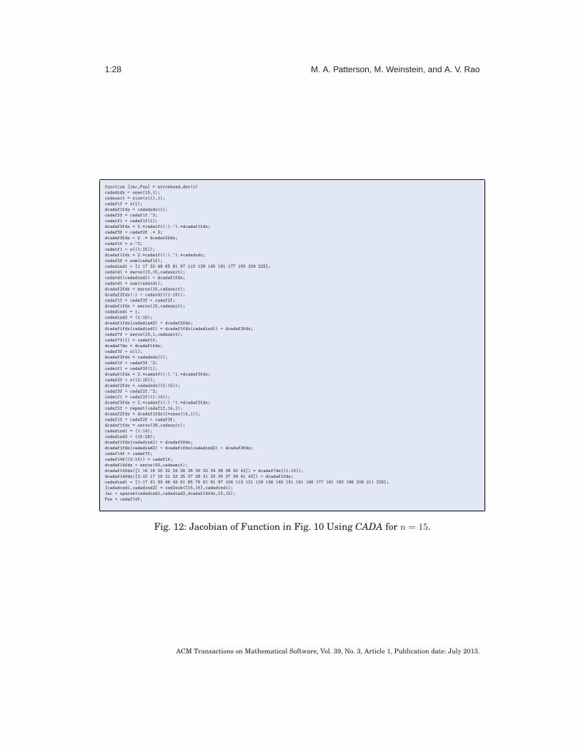
1:28 M. A. Patterson, M. Weinstein, and A. V. Rao
function [Jac,Fun] = arrowhead_der(x)
cadadxdx = ones(15,1);
cadaunit = size(x(1),1);
cadaf1f = x(1);
dcadaf1fdx = cadadxdx(1);
cadaf2f = cadaf1f.^2;
cadatf1 = cadaf1f(1);
dcadaf2fdx = 2.*cadatf1(:).^1.*dcadaf1fdx;
cadaf3f = cadaf2f .* 2;
dcadaf3fdx = 2 .* dcadaf2fdx;
cadaf1f = x.^2;
cadatf1 = x((1:15));
dcadaf1fdx = 2.*cadatf1(:).^1.*cadadxdx;
cadaf2f = sum(cadaf1f);
cadadind1 = [1 17 33 49 65 81 97 113 129 145 161 177 193 209 225];
cadatd1 = zeros(15,15,cadaunit);
cadatd1(cadadind1) = dcadaf1fdx;
cadatd1 = sum(cadatd1);
dcadaf2fdx = zeros(15,cadaunit);
dcadaf2fdx(:) = cadatd1((1:15));
cadaf1f = cadaf3f + cadaf2f;
dcadaf1fdx = zeros(15,cadaunit);
cadadind1 = 1;
cadadind2 = (1:15);
dcadaf1fdx(cadadind2) = dcadaf2fdx;
dcadaf1fdx(cadadind1) = dcadaf1fdx(cadadind1) + dcadaf3fdx;
cadaf7f = zeros(15,1,cadaunit);
cadaf7f(1) = cadaf1f;
dcadaf7dx = dcadaf1fdx;
cadaf3f = x(1);
dcadaf3fdx = cadadxdx(1);
cadaf1f = cadaf3f.^2;
cadatf1 = cadaf3f(1);
dcadaf1fdx = 2.*cadatf1(:).^1.*dcadaf3fdx;
cadaf2f = x((2:15));
dcadaf2fdx = cadadxdx((2:15));
cadaf3f = cadaf2f.^2;
cadatf1 = cadaf2f((1:14));
dcadaf3fdx = 2.*cadatf1(:).^1.*dcadaf2fdx;
cadaf2f = repmat(cadaf1f,14,1);
dcadaf2fdx = dcadaf1fdx(1*ones(14,1));
cadaf1f = cadaf2f + cadaf3f;
dcadaf1fdx = zeros(28,cadaunit);
cadadind1 = (1:14);
cadadind2 = (15:28);
dcadaf1fdx(cadadind1) = dcadaf2fdx;
dcadaf1fdx(cadadind2) = dcadaf1fdx(cadadind2) + dcadaf3fdx;
cadaf14f = cadaf7f;
cadaf14f((2:15)) = cadaf1f;
dcadaf14fdx = zeros(43,cadaunit);
dcadaf14fdx([1 16 18 20 22 24 26 28 30 32 34 36 38 40 42]) = dcadaf7dx((1:15));
dcadaf14fdx([2:15 17 19 21 23 25 27 29 31 33 35 37 39 41 43]) = dcadaf1fdx;
cadadind1 = [1:17 31 33 46 49 61 65 76 81 91 97 106 113 121 129 136 145 151 161 166 177 181 193 196 209 211 225];
[cadadind1,cadadind2] = ind2sub([15,15],cadadind1);
Jac = sparse(cadadind1,cadadind2,dcadaf14fdx,15,15);
Fun = cadaf14f;
Fig. 12: Jacobian of Function in Fig. 10 Using CADA for n = 15.
ACM Transactions on Mathematical Software, Vol. 39, No. 3, Article 1, Publication date: July 2013.

An Efficient Overloaded Method for Computing Derivatives in MATLAB 1:29
Example 3: Brown Function
Consider the following function taken from the MATLAB optimization toolbox [Math-works 2010]:
f(x) =n−1∑
i=1
[
(x2i )
x2i+1+1 + (x2
i+1)x2i+1
]
, (11)
where x = (x1, . . . , nn) ∈ Rn and f : Rn −→ R. It is known that the Hessian of the
function in Eq. (11), Hf ≡ Hf(x) = ∂2f/∂x2, is sparse. The sparsity pattern of Hf isshown in Fig. 13 for n = 8 where it is seen that the nonzero elements of the Hessianlie on the main diagonal, the sub-diagonal, and super-diagonal. The objectives of thisexample are (a) to analyze the efficiency with with CADA generates the Hessian ofEq. (11); (b) compare the efficiency which which CADA evaluates the resulting Hessianfile against INTLAB [Rump 1999], ADMAT [Coleman and Verma 1998a], and MAD[Forth 2006]; and (c) to compare the efficiency of generating second derivatives againstthe first derivative results obtained in Example 1.
struct(Hf) =
• •
• • •
• • •
• • •
• • •
• • •
• • •
• •
Fig. 13: Hessian Sparsity Pattern, struct(Hf), of Example 3 [Eq. (11)] for n = 8.
Table II shows the derivative code generation time using CADA alongside theHessian-to-function computation time ratio, CPU(Hf)/CPU(f), using CADA, INT-LAB, ADMAT, and MAD. Unlike Example 1, where the behavior in the first derivativeJacobian-to-function ratio was different for each tool, in this example it is seen thatCPU(Hf)/CPU(f) increases as a function of n using any of the automatic differenti-ation tools. Despite the fact that CPU(Hf)/CPU(f) increases with n using any of thesoftware programs, it is seen that CPU(Hf)/CPU(f) is significantly larger using eitherADMAT or MAD than it is using either CADA or INTLAB. Different from the resultof Example 1, where the efficiency of INTLAB increased with n, in this case the effi-ciency of INTLAB decreases with n because the increased computational complexityassociated with direct implementation of the rules for computing a second derivative.In the case of either ADMAT or MAD, the computational cost of computing the Hes-sian of f(x) is much higher than the cost of computing a comparable sparse Jacobianbecause both ADMAT and MAD incur additional overhead due to operator overloadingat the second derivative level. As a result, while INTLAB is less efficient in computinga sparse Hessian than it is computing a sparse Jacobian, INTLAB is still more effi-cient than either ADMAT or MAD because it is performing purely sparse arithmeticto compute the Hessian. Different from any of the other tools, CADA generates twoseparate derivative files [the first file generated computes the gradient of f(x) whilethe second file generated computes the Hessian of f(x)]. As a result, the computationalcomplexity of the Hessian derivative code is only as complex as the number of oper-ations required to compute sparsely the first derivative of the gradient (that is, theHessian of the original function).
ACM Transactions on Mathematical Software, Vol. 39, No. 3, Article 1, Publication date: July 2013.

1:30 M. A. Patterson, M. Weinstein, and A. V. Rao
Table II: CADA Derivative Generation Time and Hessian-to-Function ComputationTime Ratio, CPU(Hf)/CPU(f), for Example 3 Using CADA, INTLAB, ADMAT andMAD. The Derivative Generation Time Using CADA Was Obtained by Averaging Over100 Evaluations on a CADA Instance, While CPU(Hf)/CPU(f) Was Obtained By Av-eraging the Values Obtained Over 1000 Jacobian and Function Evaluations.
Derivative Code CPU(Hf)/CPU(f) CPU(Hf)/CPU(f) CPU(Hf)/CPU(f) CPU(Hf)/CPU(f)n Generation Time Ratio Using Ratio Using Ratio Using Ratio Using
Using CADA (s) CADA INTLAB ADMAT MAD
10 0.184 18.8 128.7 509.8 366.520 0.226 24.3 127.8 522.4 359.540 0.277 58.0 127.7 534.3 383.680 0.396 89.9 128.3 599.7 389.2160 0.655 129.1 143.1 683.9 529.2320 1.142 189.2 230.3 846.2 1101.6640 2.146 310.9 336.4 1236.3 3159.6
1280 4.331 547.1 715.9 2150.0 8143.5
Example 4: Sparse Nonlinear Programming
Consider the following sparse nonlinear programming problem (NLP) that arises fromthe discretization of the optimal control problem given on pages 247–253 of Betts[2009] using an hp–adaptive [Darby et al. 2011a; 2011b] version of the Radau pseu-dospectral method [Benson et al. 2006; Garg et al. 2010; Garg et al. 2011a; Garg et al.2011b; Patterson and Rao 2012; Rao et al. 2010; Rao et al. 2011]. The NLP decisionvector x ∈ R
8N+7 is given as
x = (x1,x2,x3,x4,x5,x6,w1,w2, κ), (12)
where N is a parameter that defines the total number of Legendre-Gauss-Radau (LGR)points [Abramowitz and Stegun 1965], xi = (x1,i, . . . , xN+1,i), (i = 1, . . . , 6), and wi =(w1,i, . . . , wN,i), (i = 1, 2). The objective of the NLP is to minimize the cost function
J = −xN+1,3 (13)
subject to the nonlinear algebraic constraints∗
N+1∑
k=1
Di,kxk,1 −κ
2xi,4 sinxi,5 = 0,
N+1∑
k=1
Di,kxk,2 −κ
2
xi,4 cosxi,5 sinxi,6
xi,1 cosxi,3
= 0,
N+1∑
k=1
Di,kxk,3 −κ
2
x4,i cosxi,5 cosxi,6
xi,1
= 0,
N+1∑
k=1
Di,kxk,4 −κ
2
[
−αPi exp[−β(xi,1 − 1)]x2i,4 −
sinxi,5
x2i,1
]
= 0,
N+1∑
k=1
Di,kxk,5 −κ
2
[
αQi exp[−β(xi,1 − 1)]xi,4 coswi,1 +
(
xi,4 −1
xi,1xi,4
)
cosxi,5
x1,i
]
= 0,
N+1∑
k=1
Di,kxk,6 −κ
2
[
αQi exp[−β(xi,1 − 1)]xi,4 sinwi,1
cosxi,5
+xi,4 cosxi,5 sinxi,6 tanxi,3
xi,1
]
= 0,
(14)
∗In order to maximize computational efficiency in MATLAB, the algebraic constraints given in Eq. (14)are implemented in a vectorized manner. As a result, the derivative files produced by CADA are the samenumber of lines regardless of the value of N used to solve this problem.
ACM Transactions on Mathematical Software, Vol. 39, No. 3, Article 1, Publication date: July 2013.

An Efficient Overloaded Method for Computing Derivatives in MATLAB 1:31
and the equality constraints
x1,1 − u1 = 0 , x1,2 − u2 = 0 , x1,3 − u3 = 0 ,
x1,4 − u4 = 0 , x1,5 − u5 = 0 ,
x1,6 − u6 = 0 , xN+1,1 − u7 = 0 ,
xN+1,4 − u8 = 0 , xN+1,5 − u9 = 0,
(15)
where u1 = 1.01248, u2 = 0, u3 = 0, u4 = 0.986496, u5 = −0.0174533, u6 = 1.57080,u7 = 1.00383, u8 = 0.0963375, u9 = −0.0872664, α = 10596.2, β = 878.273, µ0 = −0.20704,µ1 = 1.67556, γ0 = 0.07854, γ1 = −0.352896, γ2 = 2.03996, and Di,k, (i = 1, . . . , N, k =1, . . . , N + 1) is the Radau pseudospectral differentiation matrix (see Appendix A orPatterson and Rao [2012]),
Pi = γ0 + γ1wi,2 + γ2w2i,2 , Qi = µ0 + µ1wi,2. (16)
and (i = 1, . . . , N) in Eqs. (14) and (16). The total number of LGR points, N = NkK,is obtained by dividing the problem into K mesh intervals using Nk LGR points ineach mesh interval (for details see Patterson and Rao 2012). The details of the matrixDi,k, (i = 1, . . . , N, k = 1, . . . , N + 1) are given in Appendix A.
The NLP defined in Eqs. (13) and (14) can be written in the following more genericmathematical form. Determine the decision vector z ∈ R
n that minimizes the objectivefunction
f(z) (17)
subject to the nonlinear equality constraints
g(z) = 0 (18)
and the simple bounds on the decision variables
zmin ≤ z ≤ zmax. (19)
We divide the analysis in this example into two parts. First, we study the efficiencywith which CADA generates and computes the constraint Jacobian, ∂g/∂z, and theLagrangian Hessian, ∂2L/∂z2, where L = σf(z) + λ
Tg(z) and the variables σ ∈ R andλ ∈ R
6N are the Lagrange multipliers for the cost and the constraints, respectively[where we note that λ ∈ R
6N because the NLP contains 6N nonlinear constraints asshown in Eq. (14)]. Second, we demonstrate the efficiency of CADA in solving the NLPfor various values of N . In order to incorporate both first and second derivatives, inthis research the NLP was solved was solved using the second-derivative open-sourceNLP solver IPOPT [Biegler and Zavala 2008; Waechter and Biegler 2006] with theindefinite sparse symmetric linear solver MA57 [Duff 2004]. As a second derivativeNLP solver, IPOPT requires the user to supply the objective function gradient, ∂f/∂z,the constraint Jacobian, ∂g/∂z, the Lagrangian Hessian, ∂2L/∂z2, the sparsity patternof the constraint Jacobian, and the sparsity pattern of the lower-triangular portion ofthe Lagrangian Hessian.
We analyze the efficiency of CADA in a manner similar to that which was used inExamples 1–3. In order to analyze efficiency as the NLP grows in size, in this examplewe fix the number of LGR points in each mesh interval to four (that is, Nk = 4) and wevary the number of mesh intervals K. Thus, in this example the total number of LGRpoints is N = 4K. Table III shows the Jacobian-to-function ratio, CPU(Jg)/CPU(g),for the NLP constraint function of Eq. (14 as a function of N . It is seen that the ratioCPU(Jg)/CPU(g) using CADA is smaller than any of the other methods for all valuesof N except N = 128. In the case N = 128, INTLAB is slightly more efficient thanCADA in generating the constraint Jacobian, but CADA is more efficient than either
ACM Transactions on Mathematical Software, Vol. 39, No. 3, Article 1, Publication date: July 2013.

1:32 M. A. Patterson, M. Weinstein, and A. V. Rao
ADMAT or MAD. Furthermore, consistent with the results obtained in the Arrowheadfunction of Example 1, it is seen that CPU(Jg)/CPU(g) increases with N using CADA,decreases using INTLAB, and remains essentially constant using either ADMAT orMAD. Table IV shows the Hessian-to-function ratio, CPU(HL)/CPU(L), for the La-grangian Hessian L = σf(z) +λ
Tg(z). In the case of the Hessian Lagrangian it is seenthat CADA is more efficient than INTLAB and is significantly more efficient than ei-ther ADMAT or MAD for all values of N . It is interesting to see for N = 128 that theratios CPU(HL)/CPU(L) using ADMAT and MAD are approximately 15 and 50 timeshigher, respectively, when compared against CADA.
We now turn our attention to the solution of the aforementioned NLP using CADA,INTLAB, ADMAT, and MAD with the NLP solver IPOPT. While INTLAB and MADare designed to utilize forward mode automatic differentiation, ADMAT can be appliedusing either forward or reverse mode. Because the NLP of Eqs. (13) and (14) consists ofa large number of functions (that is, a large number of outputs), we choose the forwardmode option when using ADMAT. Next, because IPOPT requires that the user providethe constraint Jacobian and Lagrangian Hessian sparsity patterns, it was necessary toconstruct these patterns prior to solving the NLP. While it is possible to determine theJacobian and Lagrangian Hessian sparsity patterns with ADMAT, we found the pro-cess for determining the Hessian sparsity pattern to be unacceptably slow. In addition,INTLAB does not have a built-in capability of determining either Jacobian or Hes-sian sparsity patterns. As a result, the approach used in this research was to use theconstraint Jacobian and Lagrangian Hessian sparsity patterns that CADA generatessimultaneous with its generation of the Jacobian and Hessian derivative functions.These sparsity patterns were then supplied to IPOPT for use with all three auto-matic differentiation programs. Finally, it is noted that the constraint Jacobian wasdetermined by differentiating Eq. (14). On the other hand, it is known that the termsEq. (14) involving the coefficients Di,k, (i = 1, . . . , N, j = 1, . . . , N +1) are linear in thedecision vector. Consequently, the second derivatives of these terms are zero and, thus,will not appear in the Lagrangian Hessian. Thus, the terms involving the coefficientsDi,k, (i = 1, . . . , N, j = 1, . . . , N + 1) are not included in the computation of the NLPLagrangian.
The NLP given in Eqs. (13)–(15) was solved using IPOPT for K = (8, 16, 32, 64, 128)with Nk = 4, (k = 1, . . . ,K) (that is, the same number of Legendre-Gauss-Radau points[Abramowitz and Stegun 1965] was used in every mesh interval) with the followinginitial guess:
{x1,1, · · · , xN+1,1} = linspace(u1, u7, N + 1){x1,2, . . . , xN+1,2} = linspace(u1, u2, N + 1){x1,3, . . . , xN+1,3} = linspace(u3, u3, N + 1){x1,4, · · · , xN+1,4} = linspace(u4, u8, N + 1){x1,5, · · · , xN+1,5} = linspace(u5, u9, N + 1){x1,6, . . . , xN+1,6} = linspace(u6, u6, N + 1){w1,1, . . . , xN,1} = linspace(0, 0, N){w1,2, . . . , xN,2} = linspace(0, 0, N)
κ = 1.241475432154217,
where the function linspace(a, b,M) provides a set of M linearly equally-spaced pointsbetween a to b. The solution obtained for this problem (which matches the solu-tion in Betts [2009]) is shown in Fig. 14 for K = 16, where the NLP decision vec-tor, x, is decomposed as given by Eq. (12). Using this decomposition of x, the vec-tors (x1,j , . . . , xN+1,j), (j = 1, . . . , 6) are plotted as a function of (s1, . . . , sN+1), where(s1, . . . , sN ) are the N LGR points on the interval [−1,+1) and sN+1 = +1, while thevectors (w1,j , . . . , xN,j), (j = 1, 2) are plotted against the LGR points (s1, . . . , sN ). The
ACM Transactions on Mathematical Software, Vol. 39, No. 3, Article 1, Publication date: July 2013.

An Efficient Overloaded Method for Computing Derivatives in MATLAB 1:33
computational results obtained for this example are shown in Tables V and VI (wherethe derivative code generation time includes the post-processing step that reduces thenumber of MATLAB variables). As might be expected, the derivative code generationtime using CADA increases with K. In addition, it is seen that the time required tosolve the NLP (excluding the time required to create the derivative files) using CADAis smaller than the corresponding computation time required by either INTLAB orADMAT. Next, it is seen for K = (8, 16) that the total computation time (that is, thederivative code generation time plus the time to solve the NLP) using derivatives ob-tained by CADA is slightly larger than the solution time required by either of theother automatic differentiators. On the other hand, for the larger values of K (thatis, K = (32, 64, 128)), the total computation time using CADA is significantly less thaneither INTLAB or ADMAT. Thus, CADA becomes more computationally attractive asthe size of the NLP increases.
Another interesting advantage of CADA over either INTLAB or ADMAT pertainsto the determination of the constraint Jacobian and Lagrangian Hessian sparsity pat-terns required by IPOPT. It is known that INTLAB does not have a built-in ability tocompute sparsity patterns, while the sparsity pattern generator using ADMAT is quiteinefficient (particularly when determining the sparsity pattern of the Lagrangian Hes-sian). Thus, neither INTLAB nor ADMAT is a practical option for determining sparsitypatterns. As a result, this example demonstrates that CADA is not only efficient forgenerating derivatives, but serves the dual purpose that it is capable of efficiently gen-erating the required sparsity patterns.
Table III: CADA Derivative Generation Time and Jacobian-to-Constraint Computa-tion Time Ratio, CPU(Jg)/CPU(g), for Example 4 Using CADA, INTLAB, ADMAT andMAD. Derivative Generation Times Using CADA Were Averaged Over 100 File Gener-ations, While CPU(Jg)/CPU(g) Was Obtained by Averaging the Values Obtained Over1000 Jacobian and Function Evaluations.
Derivative Code CPU(Jg)/CPU(g) CPU(Jg)/CPU(g) CPU(Jg)/CPU(g) CPU(Jg)/CPU(g)K N = 4K Generation Time Ratio Using Ratio Using Ratio Using Ratio Using
Using CADA (s) CADA INTLAB ADMAT MAD
8 32 0.493 10.0 56.7 62.9 80.516 64 0.798 14.1 56.3 63.7 78.232 128 1.397 18.8 53.2 67.2 97.164 256 2.611 27.4 49.3 67.3 86.3128 512 5.090 49.3 45.2 68.8 72.8
Table IV: CADA Derivative Generation Time and Lagrangian Hessian to LagrangianComputation Time Ratio, CPU(HL)/CPU(L) for Example 4 Using CADA, INTLAB,ADMAT and MAD. Derivative Generation Times Using CADA Were Averaged Over100 File Generations, While CPU(HL)/CPU(L) Was Obtained by Averaging the ValuesObtained Over 1000 Lagrangian Hessian and Lagrangian Function Evaluations.
Hessian Code CPU(HL)/CPU(L) CPU(HL)/CPU(L) CPU(HL)/CPU(L) CPU(HL)/CPU(L)K N = 4K Generation Time Ratio Using Ratio Using Ratio Using Ratio Using
Using CADA (s) CADA INTLAB ADMAT MAD
8 32 2.749 84.5 253.7 1862 196516 64 4.557 154.9 344.8 2245 312032 128 8.189 272.8 904.4 3070 822764 256 15.49 512.4 2220 5604 21452128 512 30.81 1145 5191 16565 57968
ACM Transactions on Mathematical Software, Vol. 39, No. 3, Article 1, Publication date: July 2013.

1:34 M. A. Patterson, M. Weinstein, and A. V. Rao
Table V: IPOPT Solution Times for Example 4 Using Derivatives Supplied by CADA,INTLAB, ADMAT, and MAD.
Derivative Code IPOPT IPOPT IPOPT IPOPTK N = 4K Generation Time Run Time Run Time Run Time Run Time
Using CADA (s) Using CADA (s) Using INTLAB (s) Using ADMAT (s) Using MAD (s)
8 32 3.63 2.81 5.89 20.91 21.1416 64 5.67 4.53 7.38 29.13 35.6732 128 9.92 10.85 22.31 54.43 142.5964 256 18.19 25.08 69.78 163.08 499.12128 512 35.15 70.65 276.10 1088.24 25101.00
Table VI: Problem Size and Densities of Constraint Jacobian and Lagrangian HessianMatrices for Example 4.
NLP NLP Jacobian Jacobian Hessian HessianK N = 4K Variables Constraints Non-Zeros Density (%) Non-Zeros Density (%)
8 32 263 192 1920 1.92 992 1.43416 64 519 384 3840 1.92 1984 0.73732 128 1031 768 7680 0.970 3968 0.37364 256 2055 1536 15360 0.487 7936 0.188128 512 4103 3072 30720 0.244 15872 0.094
ACM Transactions on Mathematical Software, Vol. 39, No. 3, Article 1, Publication date: July 2013.

An Efficient Overloaded Method for Computing Derivatives in MATLAB 1:35
(s1, . . . , sN+1)
(x1,1,...,x
N+1,1)
-1 -0.5 0 0.51
1
1.005
1.01
1.015
(a) (x1,1, . . . , xN+1,1)vs. (s1, . . . , sN+1).
(s1, . . . , sN+1)
(x1,2,...,x
N+1,2)
-1 -0.50
0
0.2
0.4
0.5
0.6
0.8
1
1
1.2
1.4
(b) (x1,2, . . . , xN+1,2)vs. (s1, . . . , sN+1).
(s1, . . . , sN+1)
(x1,3,...,x
N+1,3)
-1 -0.50
0
0.1
0.2
0.4
0.5
0.5
0.6
0.7
1
0.3
(c) (x1,3, . . . , xN+1,3)vs. (s1, . . . , sN+1).
(s1, . . . , sN+1)
(x1,4,...,x
N+1,4)
-1 -0.50
0
0.1
0.2
0.4
0.5
0.5
0.6
0.7
0.8
0.9
1
1
0.3
(d) (x1,4, . . . , xN+1,4)vs. (s1, . . . , sN+1).
(s1, . . . , sN+1)
(x1,5,...,x
N+1,5)
0.02
-0.1
-0.08
-0.06
-0.04
-0.02
-1 -0.5
0
0 0.5 1
(e) (x1,5, . . . , xN+1,5)vs. (s1, . . . , sN+1).
(s1, . . . , sN+1)
(x1,6,...,x
N+1,6)
-1 -0.50
0
0.2
0.4
0.5
0.6
0.8
1
1
1.2
1.4
1.6
(f) (x1,6, . . . , xN+1,6)vs. (s1, . . . , sN+1).
−1.4
−1.2
(s1, . . . , sN)
(w1,1,...,w
N,1)
-0.2
-0.4
-0.6
-0.8
-1
-1 -0.5
0
0 0.5 1
(g) (w1,1, . . . , wN,1) vs. (s1, . . . , sN ).
(s1, . . . , sN)
(w1,2,...,w
N,2)
-1 -0.5 0 0.5 10.29
0.295
0.3
0.305
0.31
(h) (w1,2, . . . , wN,2) vs. (s1, . . . , sN ).
Fig. 14: Components of NLP Decision Vector for Example 4 with K = 16.
ACM Transactions on Mathematical Software, Vol. 39, No. 3, Article 1, Publication date: July 2013.

1:36 M. A. Patterson, M. Weinstein, and A. V. Rao
6. DISCUSSION
The four examples given in Sections 5 demonstrate three different aspects of CADA.Example 1 demonstrated the ability for CADA to avoid expression explosion that couldpossibly result in an exhaustion of memory by greatly reducing the number of vari-ables created in the workspace when executing the final derivative file. In addition,it was seen in Example 1 that, despite the large number of function evaluations, thecode produced by CADA was obtained and executed efficiently when compared againstthe MATLAB Symbolic Math Toolbox. Example 2 demonstrated the efficiency withwhich CADA generates the first derivative of a function whose Jacobian is sparse andcompares the efficiency of the CADA-generated derivative code against the leading au-tomatic differentiation software INTLAB, ADMAT, and MAD. Example 2 also demon-strated how CADA takes advantage of vectorization in the original function code bycreating a vectorized derivative code that contains the same number of lines of coderegardless of the value of n used to compute the original function. Finally, Example 2demonstrated that CADA generates a sparse representation of the derivative, comput-ing only the nonzero derivatives and storing only the indices corresponding to thesenon-zeros. Lastly, it was found in this second example that the CADA derivative codegeneration time grew quite slowly due to the fact that the derivative computationstook advantage of vectorization and sparsity. Example 3 demonstrated the efficiencywith which CADA generates the Hessian of a scalar function of a vector. This thirdexample highlighted the fact that CADA is more efficient than INTLAB and is signif-icantly more efficient than either ADMAT or MAD. This increased second derivativeefficiency in CADA over the other automatic differentiation software is particularly no-ticeable as the function size gets large. Example 4 showed how CADA could be used ona potentially more practical problem of solving a large sparse nonlinear programmingproblem (NLP). This fourth example demonstrated not only the efficiency with whichCADA can create and evaluate the first and second derivatives required by the NLP,but also highlighted the feature that CADA can generate the exact sparsity patternfor these required derivatives. It was also found in Example 4 that CADA comparedfavorably against two other well known and commonly used automatic differentiationtools.
7. LIMITATIONS OF CADA
While the examples show several key advantages of the current approach, we nowdiscuss some limitations of the method. First, it is not possible in the present formto differentiate functions that contain conditional statements of CADA objects (for ex-ample, if and while statements) because the overloaded approach does not operateon numerical values of the input. Second, similar to the limitation pertaining to con-ditional statements, for loops with statements that include CADA objects can not bedifferentiated because the overloaded object does not contain numerical values. It isnoted, however, that functions where a for loop does not contain a CADA object canbe differentiated. In this latter case, the derivative function will not contain any forloops, but instead will produce a sequence of statements that executes each iterationof the loop. Finally, the derivative code generated using CADA depends upon the sizesof the variables specified when differentiating the function. Moreover, if it is desired tofind derivatives of that same function using different sizes of the input variables, thefunction must be differentiated again using the new variable sizes, generating a newderivative code.
ACM Transactions on Mathematical Software, Vol. 39, No. 3, Article 1, Publication date: July 2013.

An Efficient Overloaded Method for Computing Derivatives in MATLAB 1:37
8. CONCLUSIONS
An object-oriented method has been described for computing derivatives of MATLABfunctions. A new class called CADA has been developed. The derivatives of a generalfunction can be obtained by evaluating a function of interest on a CADA object andwriting the derivatives to a file that itself can be executed. The derivative file containsthe same sequence of operations as the forward mode of automatic differentiation.Moreover, because the derivative function has the same input as the original functioncomputer code, it is possible to apply the method recursively to generate higher-orderderivatives. As a result, the method provides the ease of use associated with forwardmode automatic differentiation while simultaneously providing the same functionalityas would be obtained had the analytic derivatives been coded by hand. The key com-ponents of the method have been described in detail and the usability of the methodwas demonstrated on four examples, where each example exercised different aspectsof the method. The method presented in this paper provides an efficient and reliableapproach for computing analytic derivatives of general MATLAB functions.
REFERENCES
ABRAMOWITZ, M. AND STEGUN, I. 1965. Handbook of Mathematical Functions with Formulas, Graphs, andMathematical Tables. Dover Publications, New York.
BENSON, D. A., HUNTINGTON, G. T., THORVALDSEN, T. P., AND RAO, A. V. 2006. Direct trajectory opti-mization and costate estimation via an orthogonal collocation method. Journal of Guidance, Control,and Dynamics 29, 6, 1435–1440.
BETTS, J. T. 2009. Practical Methods for Optimal Control and Estimation Using Nonlinear Programming.SIAM Press, Philadelphia.
BIEGLER, L. T. AND ZAVALA, V. M. 2008. Large-scale nonlinear programming using IPOPT: An integratingframework for enterprise-wide optimization. Computers and Chemical Engineering 33, 3, 575–582.
BISCHOF, C. H., BÜCKER, H. M., LANG, B., RASCH, A., AND VEHRESCHILD, A. 2002. Combining sourcetransformation and operator overloading techniques to compute derivatives for MATLAB programs. InProceedings of the Second IEEE International Workshop on Source Code Analysis and Manipulation(SCAM 2002). IEEE Computer Society, Los Alamitos, CA, USA, 65–72.
BISCHOF, C. H., CARLE, A., CORLISS, G. F., GRIEWANK, A., AND HOVLAND, P. D. 1992. ADIFOR: Gener-ating derivative codes from Fortran programs. Scientific Programming 1, 1, 11–29.
BISCHOF, C. H., CARLE, A., KHADEMI, P., AND MAUER, A. 1996. ADIFOR 2.0: Automatic differentiationof Fortran 77 programs. IEEE Computational Science & Engineering 3, 3, 18–32.
CAYUGA RESEARCH 2008–2009. ADMAT: Automatic Differentiation Toolbox User’s Guide, Version 2.0.CAYUGA RESEARCH.
COLEMAN, T. F. AND VERMA, A. 1998a. ADMAT: An Automatic Differentiation Toolbox for MATLAB. Tech-nical Report. Computer Science Department, Cornell University.
COLEMAN, T. F. AND VERMA, A. 1998b. ADMIT-1: Automatic differentiation and MATLAB interface tool-box. ACM Transactions on Mathematical Software 26, 1, 150–175.
DARBY, C. L., HAGER, W. W., AND RAO, A. V. 2011a. Direct trajectory optimization using a variable low-order adaptive pseudospectral method. Journal of Spacecraft and Rockets 48, 3, 433–445.
DARBY, C. L., HAGER, W. W., AND RAO, A. V. 2011b. An hp–adaptive pseudospectral method for solvingoptimal control problems. Optimal Control Applications and Methods 32, 4, 476–502.
DOBMANN, M., LIEPELT, M., AND SCHITTKOWSKI, K. 1995. Algorithm 746: PCOMP: A Fortran code forautomatic differentiation. ACM Transactions on Mathematical Software 21, 3, 233–266.
DUFF, I. S. 2004. MA57—a code for the solution of sparse symmetric definite and indefinite systems. ACMTransactions on Mathematical Software 30, 2, 118–144.
FORTH, S. A. 2006. An efficient overloaded implementation of forward mode automatic differentiation inMATLAB. ACM Transactions on Mathematical Software 32, 2, 195–222.
FORTH, S. A., TADJOUDDINE, M., PRYCE, J. D., AND REID, J. K. 2004. Jacobian code generated by sourcetransformation and vertex elimination can be as efficient as hand–coding. ACM Transactions on Math-ematical Software 30, 4, 266–299.
GARG, D., HAGER, W. W., AND RAO, A. V. 2011a. Pseudospectral methods for solving infinite-horizon opti-mal control problems. Automatica 47, 4, 829–837.
ACM Transactions on Mathematical Software, Vol. 39, No. 3, Article 1, Publication date: July 2013.

1:38 M. A. Patterson, M. Weinstein, and A. V. Rao
GARG, D., PATTERSON, M. A., DARBY, C. L., FRANCOLIN, C., HUNTINGTON, G. T., HAGER, W. W., AND
RAO, A. V. 2011b. Direct trajectory optimization and costate estimation of finite-horizon and infinite-horizon optimal control problems via a Radau pseudospectral method. Computational Optimization andApplications 49, 2, 335–358.
GARG, D., PATTERSON, M. A., HAGER, W. W., RAO, A. V., BENSON, D. A., AND HUNTINGTON, G. T. 2010. Aunified framework for the numerical solution of optimal control problems using pseudospectral methods.Automatica 46, 11, 1843–1851.
GRIEWANK, A. 2008. Evaluating Derivatives: Principles and Techniques of Algorithmic Differentiation.Frontiers in Appl. Mathematics. SIAM Press, Philadelphia, Pennsylvania.
GRIEWANK, A., JUEDES, D., AND UTKE, J. 1996. Algorithm 755: ADOL-C, a package for the automaticdifferentiation of algorithms written in c/c++. ACM Transactions on Mathematical Software 22, 2, 131–167.
HASCOËT, L. AND PASCUAL, V. 2004. TAPENADE 2.1 user’s guide. Rapport Technique 300, INRIA, SophiaAntipolis.
KHARCHE, R. V. 2011. Matlab automatic differentiation using source transformation. Ph.D. thesis, Depart-ment of Informatics, Systems Engineering, Applied Mathematics, and Scientific Computing, CranfieldUniversity.
KHARCHE, R. V. AND FORTH, S. A. 2006. Source transformation for MATLAB automatic differentiation. InComputational Science – ICCS, Lecture Notes in Computer Science, V. N. Alexandrov, G. D. van Albada,P. M. A. Sloot, and J. Dongarra, Eds. Vol. 3994. Springer, Heidelberg, Germany, 558–565.
LANTOINE, G., RUSSELL, R. P., AND DARGENT, T. 2012. Using multicomplex variables for automatic com-putation of high-order derivatives. ACM Transactions on Mathematical Software 38, 3, 16:1–16:21.
MARTINS, J. R. R. A., STURDZA, P., AND ALONSO, J. J. 2003. The complex-step derivative approximation.ACM Transactions on Mathematical Software 29, 3, 245–262.
MATHWORKS. 2010. Version R2010b. The MathWorks Inc., Natick, Massachusetts.MONAGAN, M. B., GEDDES, K. O., HEAL, K. M., LABAHN, G., VORKOETTER, S. M., MCCARRON, J., AND
DEMARCO, P. 2005. Maple 10 Programming Guide. Maplesoft, Waterloo ON, Canada.NEIDINGER, R. D. 2010. Introduction to Automatic Differentiation and MATLAB Object-Oriented Program-
ming. SIAM REVIEW 52, 3, 545–563.PADULO, M., FORTH, S. A., , AND GUENOV, M. D. 2008. Robust aircraft conceptual design using auto-
matic differentiation in matlab. In Advances in Automatic Differentiation, C. H. Bischof, H. M. BÃijcker,P. Hovland, U. Naumann, J. Utke, T. J. Barth, M. Griebel, D. E. Keyes, R. M. Nieminen, D. Roose, andT. Schlick, Eds. Lecture Notes in Computational Science and Engineering Series, vol. 64. Springer,Berlin, Heidelberg, 271–280.
PATTERSON, M. A. AND RAO, A. V. 2012. Exploiting sparsity in direct collocation pseudospectral methodsfor solving continuous-time optimal control problems. Journal of Spacecraft and Rockets, 49, 2, 364–377.
RAO, A. V., BENSON, D. A., CHRISTOPHER DARBY, M. A. P., FRANCOLIN, C., SANDERS, I., AND HUNT-INGTON, G. T. 2010. Algorithm 902: GPOPS, A MATLAB software for solving multiple-phase optimalcontrol problems using the Gauss pseudospectral method. ACM Transactions on Mathematical Soft-ware 37, 2, 22:1–22:39.
RAO, A. V., BENSON, D. A., DARBY, C. L., MAHON, B., FRANCOLIN, C., PATTERSON, M. A., SANDERS,I., AND HUNTINGTON, G. T. 2011. User’s Manual for GPOPS Version 4.x: A MATLAB Softwarefor Solving Multiple-Phase Optimal Control Problems Using hp–Adaptive Pseudospectral Methods.http://www.gpops.org.
RUMP, S. M. 1999. Intlab – INTerval LABoratory. In Developments in Reliable Computing, T. Csendes, Ed.Kluwer Academic Publishers, Dordrecht, Germany, 77–104.
SHAMPINE, L. F. 2007. Accurate numerical derivatives in Matlab. ACM Transactions on MathematicalSoftware 33, 4, 26:1–26:17.
SPEELPENNING, B. 1980. Compiling fast partial derivatives of functions given by algorithms. Ph.D. thesis,University of Illinois at Urbana-Champaign.
TADJOUDDINE, M., FORTH, S. A., PRYCE, J. D., AND REID, J. K. 2002. Performance issues for vertex elim-ination methods in computing jacobians using automatic differentiation. In Proceedings of the Interna-tional Conference on Computational Science-Part II. ICCS ’02. Springer-Verlag, London, UK, 1077–1086.
WAECHTER, A. AND BIEGLER, L. T. 2006. On the implementation of a primal-dual interior-point filter linesearch algorithm for large-scale nonlinear programming. Mathematical Programming 106, 1, 575–582.
WOLFRAM. 2008. Mathematica Edition: Version 7.0. Wolfram Research, Inc., Champaign, Illinois.
ACM Transactions on Mathematical Software, Vol. 39, No. 3, Article 1, Publication date: July 2013.

An Efficient Overloaded Method for Computing Derivatives in MATLAB 1:39
A. COMPUTATION OF DIFFERENTIATION MATRIX IN EXAMPLE 4
The coefficients Dik, (i = 1, . . . , N, j = 1, . . . , N + 1) are defined as follows [Pat-terson and Rao 2012]. First, let s be defined on the domain [−1,+1]. Suppose fur-ther that s ∈ [−1,+1] is partitioned into K mesh intervals (S1, . . . , SK), where Sk =[sk−1, sk], (k = 1, . . . ,K) such that s0 = −1 and sK = +1. Within each mesh intervalsSk, k = (1, . . . ,K), define the following basis of Nk+1 Lagrange polynomials [Pattersonand Rao 2012]:
ℓ(k)j (s) =
Nk+1∏
l=1
l 6=j
s− s(k)l
s(k)j − s
(k)l
, k = 1, . . . ,K, (20)
where(
s(k)1 , . . . , s
(k)Nk
)
are the Nk Legendre-Gauss-Radau [Abramowitz and Stegun
1965] (LGR) collocation points in mesh interval Sk, (k = 1, . . . ,K). Next, within eachmesh intervals k, let
D(k)ij =
[
dℓ(k)j (s)
ds
]
s(k)i
, (i = 1, . . . , Nk, j = 1, . . . , Nk + 1, k = 1, . . . ,K), (21)
The matrix Dik, (i = 1, . . . , N, k = 1, . . . , N + 1) then has the followingblock structure that is comprised of the matrices defined in Eq. (21) such thatthe nonzero row-column indices in the kth block of Dik are given as (
∑k−1l=1 Nl +
1, . . . ,∑k
l=1 Nl,∑k−1
l=1 Nl + 1, . . . ,∑k
l=1 Nl + 1), where for every mesh interval k ∈[1, . . . ,K] the nonzero elements are defined by the matrix given in Eq. (21). It isnoted that the complete set of LGR points is given by (s1, . . . , sN ), where (s1, . . . , sN ) =(
(s(1)1 , . . . , s
(1)N1
), (s(2)1 , . . . , s
(2)N2
), . . . , (s(K)1 , . . . , s
(K)NK
))
, and the parameter N is defined as
N =
K∑
k=1
Nk. (22)
A schematic of the matrix Dik, (i = 1, . . . , N, k = 1, . . . , N + 1) is shown in Fig. 15.
Block 1
Block 2
Block 3
Block K
(2) Zeros Except in Blocks
(1) Block k is of Size Nk by Nk+1
(3) Total Size N by N+1
Fig. 15: Structure of Matrix Di,k, (i = 1, . . . , N, k = 1, . . . , N + 1) for Example 3.
Received December 2012; revised May 2013; accepted August 2013
ACM Transactions on Mathematical Software, Vol. 39, No. 3, Article 1, Publication date: July 2013.