An Improved Force-restore Model for Land-surface Modeling

Diandong Ren and Ming Xue

School of Meteorology and Center for Analysis and Prediction of Storms

University of Oklahoma, Norman, Oklahoma 73019

Submitted to J. of Applied Meteorology

November 2002

Revised September 2003

Corresponding Author Address: Dr. Ming Xue,

School of Meteorology, University of Oklahoma, 100 East Boyd, Norman, OK 73019.

E-mail: mxue@ou.edu.

ABSTRACT

To clarify the definition and to improve the forecast of the 'deep layer' temperature in the

soil-temperature force-restore model, the prediction equations in such a model are re-derived.

The derivation led to a deep-layer temperature, commonly denoted T2, that is defined as the soil

temperature at depth dπ plus a transient term where d is the e-folding damping depth of soil

temperature diurnal oscillations. The corresponding prediction equation for T2 has the same form

as the commonly used one except for an additional term involving the lapse rate of the 'seasonal-

mean' soil temperature and the damping depth d. A term involving the same also appears in the

skin temperature prediction equation, which also includes a transient term. The impact on the soil

temperature prediction by these additional terms are tested against the Oklahoma Atmospheric

Surface-layer Instrumentation System Project (OASIS) observations for four week-long periods

selected from four seasons in 2000.

Clear improvements in the prediction of both skin and deep layer temperature were

obtained using the revised formulation, and improvement in the latter is much more dramatic.

The inclusion the lapse-rate related terms is most significant while the transient terms can be

neglected. The addition of the lapse-rate related terms removes a drift found in the predicted

deep-layer temperature towards the mean of skin temperature. Practical application of the revised

system is also discussed.

1. Introduction

Land surface models (LSMs) deal with evolution of land surface and deep soil layer

conditions and the exchanges of moisture and thermal energy between the land surface and the

atmosphere. Land surface modeling is important for the studies of climatic predictions (e.g.,

Dickinson and Henderson-Sellers 1988), hydrology (e.g., Milly and Dunne 1994) and numerical

weather prediction (e.g., Betts et al. 1997; Chen and Dudhia 2001).

Among land surface models of various complexities, a so-called force-restore (FR) model

for soil temperature prediction is rather popular (e.g., Deardorff 1978, D78 hereafter; Noilhan

and Planton 1989, NP89 hereafter; Mahfouf et al. 1995) because of its computational efficiency

and reasonable physical foundation. It employs a minimum number of prognostic variables yet

captures the most important physical processes. The model was originally developed by

Bhumralkar (1975, B75 hereafter), and Blackadar (1976, B76 hereafter), and adopted by D78

and used in models such as ISBA (Interactions between Soil, Biosphere, and Atmosphere, NP89;

Mahfouf et al. 1995).

The force-restore model, as applied to soil temperature, usually involves two prognostic

equations, one for the surface or skin temperature (Ts) representing the temperature of both

canopy and soil surface, and the other for a temperature (T2) towards which Ts is relaxed. T2 is

defined as the mean surface temperature averaged over one day by B75. In some other modeling

studies (e.g., D78), T2 is treated as deep soil temperature, however.

In this study, the soil model in the Advanced Regional Prediction System (ARPS, Xue et

al. 1995; Xue et al. 2000; Xue et al. 2001) is tested against observed soil temperature data in

week-long periods during four different seasons. The model is based on NP89 and some of its

later modifications. Drift on the order of 5 K is found in the deep soil temperature, variable T2,

2

predicted by the model. Modifications to the temperature equations are found through re-

derivation of the equations, taking into account the change in the seasonally averaged soil

temperature with depth. In section 2, the equations as used by B75 and NP89 are first briefly

reviewed followed by derivation of a revised version. The physical meaning of T2 will also be

discussed. The Oklahoma Atmospheric Surface-layer Instrumentation System Project (OASIS,

Brotzge et al. 2001) observational data will be described in Section 3. Land surface scheme in

ARPS and the design of the numerical experiments will be discussed in Section 4. The numerical

results will be presented in Section 5 and compared with observational data. Finally, conclusions

are given in Section 6.

2. The revised force-restore model for soil temperature

a) Prognostic equations for soil temperature and the force-restore model

The equation describing the time evolution of soil temperature, T, can be written in terms

of the vertical flux convergence, assuming the effect of horizontal heat exchange can be

neglected:

T GCt z

∂ ∂= −

∂ ∂, 0z−∞ < ≤ , (1)

where G is the heat flux given by the following:

0 , 0( , )

. 0T

G zG z t TK C z

z

=⎧⎪= ∂⎨

− <⎪ ∂⎩

(2)

Here, C is the volumetric soil heat capacity (J m-3 K-1), t the time, z the vertical coordinate

(positive upward and zero at the ground surface), KT the soil thermal diffusivity (m2 s-1). KT is

related to soil thermal conductivity λ (W m-1 K-1) by soil heat capacity, i.e., KT =λ/C. G0 in

Eq.(2) is the net heat flux at the ground given by

3

0 nG LE H R= + − , (3)

where Rn is the net radiation flux at the surface which includes net short and long wave radiation.

LE is the latent heat and H the sensible heat fluxes leaving the ground surface.

For the interior of the soil, Eq.(1) becomes

( )T TCt z z

λ∂ ∂ ∂=

∂ ∂ ∂. (4)

If λ is assumed constant,

2

2

T TCt z

λ∂ ∂=

∂ ∂. (5)

Numerical integration of Eq. (4) using multiple vertical layers would allow for variable

λ , realistic initial soil temperature profiles and boundary conditions. In the case where the

vertical variation in thermal conductivity is relatively small, or little knowledge is known of its

vertical variation, a simpler and more economical model derived from Eq.(4), with λ set as

constant, can be rather accurate. The force-restore model is such a model and it was originally

developed by B75 and B76 and popularized by D78. It is used in land surface models such as

ISBA (NP89; Mahfouf et al. 1995).

In B75, the temperature at the surface is assumed to be sinusoidal with a 24-hour diurnal

cycle and is expressed as

(0, ) sin( )T t T A tω= + (6)

where ω is the frequency of oscillation (ω= 2 /π τ , withτ being the period of oscillation and

equal to 24 hours). T is defined in B75 as the daily average temperature of the soil assumed to

be the same at all depths, and A is the amplitude of temperature wave at the surface. An equation

for the mean temperature in a thin surface layer of depth d1 (taken to be 1 cm) was obtained by

B75 as follows,

4

1/ 2

0 ( )2

ss

T Cc G T Tt

ω λ∂ ⎛ ⎞= − −⎜ ⎟∂ ⎝ ⎠, (7)

where Ts is the ground surface temperature, 1 / 2c d C Cλ ω= + , and G0 is the net surface heat

flux given in Eq.(3). It is this equation or a variation of it that is used in land surface models like

that of NP89. In NP89, the definition of c is approximated by dropping the first term on the right

hand side (rhs) of its definition, i.e. term 1d C . The approximation actually originated from and

was discussed in D78, and is equivalent to assuming that the heat capacity of this thin layer is so

small that the surface heat flux into this thin layer is roughly balanced by the ground heat flux

into the deep layer.

With the above approximation or consideration, Eq. (7) becomes

0 22 ( )s

G sT C G T Tt

πτ

∂= − −

∂. (8)

where 2 /GC Cω λ≡ . When vegetation is present, this coefficient will be modified to include

the effect of vegetation on heat capacity (see, e.g., NP89). In the above equation, the daily mean

temperature, T , has been replaced by a new symbol, T2, because variable T has become a time

dependent variable to be predicted by another equation to be discussed next. Symbol T , with an

over-bar denoting time averaging, can be misleading. Equation (8), in a slightly different form,

was also tested by D78.

In NP89, a second equation is given for T , now named T2 but still defined as the daily

mean temperature. This equation is

22

1 ( )sT T Tt τ

∂= −

∂. (9)

No detail on the derivation of this equation was, however, given in NP89, except for references

to B75 and B76. Interestingly, neither B75 nor B76 provided the equation for the prediction of

5

T2. In B76, it is said that "the value to be used for θm (our T2) is the mean temperature of the

surface air during the most recent 24 hours".

The definition of T2 has not always been consistent in the literature. B75 defines it, when

it appears in the equation for surface temperature, as "the daily mean temperature at the surface

assumed to be the same at all depths". NP89 defines it in a similar way, as the mean value of Ts

over one day. D78, however, calls it the deep soil temperature, and predicts it using an equation

that is analogous to Eq.(8) but without the restore term on the rhs. In the forcing term of that

equation that corresponds to the first term on the rhs of Eq.(8), a frequency that corresponds to

annual instead of daily cycle is used. In another word, a different equation for the prediction of

T2 is used in D78 than that in NP89.

The definition of T2 has been vague even in the same ISBA community; daily mean soil

temperature is used in some papers (e.g., NP89, Mahfouf and Noilhan 1991; Noilhan and

Lacarre`re 1995; Noilhan and Mahfouf 1996; Calvet et al. 1998) and while deep soil temperature

in others (e.g., Bouttier et al. 1993; Boone et al. 2000). Different definitions can even be found in

the same article (Bouttier et al. 1993). When T2 is considered deep soil temperature, different

depths had been used. For example, Bouttier et al. (1993) considered T2 the temperature at 1 m

depth, while Calvet et al. (1998) and Mahfouf and Noilhan (1991) the temperature at 0.81 meter.

In Mahfouf and Noilhan (1991), even though T2 is defined as the mean daily temperature (page

1357) but measurement at 81 cm depth is used to initialize T2 (page 1358). These differences in

definition often lead to confusion in interpreting and verifying the model results.

One reason for the seemingly interchangeable use of daily average temperature and the

deep soil temperature may have risen from the original assumption of B75, who assumed the

daily mean temperature is the same at all depths. This assumption may be valid in the spring and

6

fall seasons, but is certainly not true in most parts of the world at summer and winter (de Vries

1963). Figure 1a shows the OASIS measurements of soil temperature at ground level, and those

at 25 and 60 cm depth for a 7-day summer period starting from 12 August 2000. The means of

these three temperature time series are respectively 306.7, 304.2 and 301.2 K, indicating a

decreasing trend with depth. The difference between the mean temperatures of skin and at 60 cm

is as large as 5.5 K for this period. A reverse trend is apparent for the winter period (a 7-day

period starting from 5 January 2000) as shown in Fig.1b, where the soil temperatures at 5, 25 and

60 cm have respective means of 280.0, 281.1 and 283.4 K. The temperature increases with depth

in this case. The above behavior appears to be also observed by Mahfouf et al. (1995) who found

for climate simulations a spurious drift towards too low temperatures, especially over continental

areas during the polar nights. Their solution to this problem with a force-restore model is to add

another term to the rhs of T2 equation that relaxes T2 towards a climatological deep soil

temperature. While it appears to work, the physical basis for doing so is not entirely clear.

In the following section, we re-derive the two equations for soil temperature and attempt

to establish a clear definition for T2 and at the same time obtain a set of equations for improved

prediction of Ts and T2, especially of the latter.

b) Revised Force-Restore Model for Soil Temperature

Here we define the seasonal mean soil temperature as the running mean of temperature

over 1-2 weeks, a period long enough to remove diurnal temperature changes while retain the

seasonal variations. In general, this temperature increases (decreases) downward in winter (

summer). Seasonal mean temperature can be considered the background upon which the diurnal

oscillations are superimposed. This temperature is similar to the mean temperature defined by

B75 except that we do not assume it constant at all depths. We will see that taking into account

7

of the vertical variation in this mean temperature introduces additional terms into the force-

restore equations.

Suppose this seasonal mean temperature profile of the soil is given by z sT T zγ= + , where

sT is the mean temperature at the surface, and γ is the “lapse rate” of the mean temperature

(positive as temperature decreases with depth). Thus, under sinusoidal surface forcing with

single dominant period, as in the form of Eq. (6), the soil temperature as a solution to Eq.(5) can

be found to be

0( , ) sin( ) ,zd

szT z t T z Ae td

γ ω φ= + + + + (10)

where 0 0tφ ω≡ is the initial phase and t0 is the time at which the amplitude of surface

temperature oscillation is zero. /Td K τ π= 2 / Cλ ω= is the e-folding damping depth

at which the amplitude of surface temperature oscillations is reduced by a factor of e-1 (about

0.37). Obviously, it is a function of soil thermal diffusivity and the period of forcing. E-folding

damping depth is much larger for annual forcing than for diurnal forcing. Higher thermal

diffusivity also results in larger damping depth.

Soil water content plays a role through its double effects on soil heat capacity and soil

thermal conductivity. It increases C, but at the same time increases λ. This makes it hard to

determine the net effects of soil moisture on KT. In general, for all types of common soil, the

largest thermal diffusivity is achieved when soil volumetric water content reaches about 25%. KT

was assumed to be constant with depth in this study as well as in B75.

The general solution for soil temperature (10) tells us that the amplitude of soil

temperature fluctuations decreases exponentially with depth and the phase delay increases

8

linearly with depth; the amplitude is dampened faster with depth for high frequency modes,

which justifies our using of only one mode (daily cycle) in the analysis.

The background soil temperature profile also implies an extra soil heat flux of constant

magnitude λγ− for all depths. Thus, at the surface (z=0), the soil heat flux

equals 0(0, )G t G λγ= − , or, a modification to the definition of Eq. (3). Plug the solution of T in

Eq. (10) into the definition of ground heat flux given in (2), we obtain

0 01( , ) sin( ) cos( ) .

zd z zG z t Ae t t

d d dλ γ ω φ ω φ

⎧ ⎫⎡ ⎤= − + + + + + +⎨ ⎬⎢ ⎥⎣ ⎦⎩ ⎭ (11)

From Eq.(10) and its time derivative we have

0sin( ) ( , ) ,zd

szA e t T z t T zd

ω φ γ+ + = − − (12)

and 01 ( , )cos( ) .

zd z T z tAe t

d tω φ

ω∂

+ + =∂

(13)

In obtaining Eq.(13), we have assumed that the time rate of change in γ is a very slow-

varying function of time, therefore its time derivative can be neglected. Plug Eqs. (12) and (13)

into Eq. (11), to obtain

1 1 ( , )( , ) ( , ) .sT z tG z t T z t T z

d tλ γ γ

ω⎧ ∂ ⎫⎡ ⎤= − + − − +⎨ ⎬⎢ ⎥∂⎣ ⎦⎩ ⎭

(14)

Applying Eq.(14) to z=0, and making use of surface energy balance equation (3), we obtain, after

some reorganization,

(0, ) 2 [ (0, )] [ ]s netT t dT T t R LE H

tπ ω

τ λ∂

= − + − −∂

(16)

where ( ) / 1/d cω λ ≈ . If we designate 1/ 2 /( )GC c dC≡ ≈ , Equation (16) can be rewritten as

(0, ) 2[ ] [ (0, )]G net sT t C R LE H T T t

tπ

τ∂

= − − + −∂

. (17)

9

Equation (17) is essentially the force-restore equation for surface temperature derived by B75

and used in models of D78 and NP89. The key issue here is the definition of the temperature

towards which the surface temperature is restored. In Eq. (17), this temperature is sT , the

temporal mean surface temperature.

In Eq.(17), sT , defined as the time mean surface temperature, is not known. It is a slow

varying quantity and we choose to relate it to a temperature of the deep layer soil of some sort.

Here we set out to derive an equation for the mean (vertically averaged) temperature of the deep

layer. The mean temperature of the layer extending from the ground level to a depth at z is

defined by 2 0

1 ( ', ) 'z

T T z t dzz

≡ ∫ . Plugging in T(z) given by Eq. (10) gives

2 0 0

0 0

[sin( ) cos( )]2 2

[sin( ) cos( )].2

zd

sz dA z zT T e t t

z d ddA t t

z

γ ω φ ω φ

ω φ ω φ

= + + + + − + +

− + − + (18)

Taking a time derivative of Eq. (18) and making use of Eq. (12), we have

20 0[sin( ) sin( )] [ ( , ) (0, ) ]

2

zdT d zAe t t T z t T t z

t z dω ω φ ω φ γ

⎧ ⎫∂= + + − + + − −⎨ ⎬∂ ⎩ ⎭

. (19)

Letting z = - πd, i.e., choosing the depth of the layer for which we look for the vertical mean to

be πd, Eq. (19) becomes

(0~ )0

1( 1)cos( ) [ ( , ) (0, ) ]2

dT A e t T d t T t dt

π πω ω φ π γππ τ

− −∂= + + − − − +

∂. (20)

Let z = - πd again, we obtain the mean temperature in the πd deep layer as

[ ](0 ) 0 0(1 ) sin( ) cos( )

2 2d sd A eT T t t

π

πγπ ω φ ω φ

π

−

−

+= − + + − +∼ . (21)

Applying Eq. (12) at z = - πd , rearranging, we have

10

0( , ) sin( ) .sT T d t A e t dzππ ω φ γπ−= − + + + (22)

Plug the above equation into Eq. (21), we obtain

(0 ) 0 0(1 ) (1 )( , ) sin( ) cos( )

2 2 2dd e A eT T d t A e t t

π ππ

πγππ ω φ ω φ

π π

− −−

−

⎡ ⎤+ += − + + + + − +⎢ ⎥

⎣ ⎦∼ . (23)

Let (1)(0~ ) 0( 1)sin( )

2 2dd AT T e tπ

ππ γ ω φ

π−

− = + + + + , (24)

where

(1)

0 0

0

(1 )( , ) cos( ) sin( )2

( , ) sin( )

A eT T d t t Ae t

T d t AB t

πππ ω φ ω φ

ππ ω φ α

−−+

= − − + + +

= − + + +. (25)

and 1 (1 )tan 0.42 ,2

ee

π

πα ππ

−−

−

⎡ ⎤− += ≈ −⎢ ⎥

⎣ ⎦ and

0.5221 0.17

2eB e

ππ

π

−−

⎡ ⎤⎛ ⎞+= + ≈⎢ ⎥⎜ ⎟

⎢ ⎥⎝ ⎠⎣ ⎦.

Plug (0~ )dT π− given in (24) into (20), making use of Eq.(13) applied at z=0, we obtain

(1)

(1)0

1 [ ( , ) (0, ) ]

1 [ (0, ) ] sin( ).

T T d t T t dt

ABT T t d t

π γπτ

γπ ω φ ατ τ

∂= − − − +

∂

= − − + + + + (26)

Equation (26) is similar to the 'deep layer' temperature equation used in traditional force-restore

models (see, e.g., NP89), except for the sine term on the rhs and dγπ term. The sine term

considerably complicates the equation. We want to see if the equation can simplified through

further variable transform. We define (1) (2)0cos( )

2ABT T tω φ απ

= − + + and plug it into (26) to

obtain

(2)

(2)0

1 [ (0, ) ] cos( )2

T ABT T t d tt

γπ ω φ ατ πτ

∂= − − + + + +

∂. (27)

11

Eq. (27) is more attractive than Eq.(26) because the last term on the rhs is a factor of 2π smaller

than that in Eq. (26). The next transform would be (2) (3)02 sin( ),

(2 )ABT T tω φ απ

= + + + and Eq.

(27) can be then rewritten as

(3)(3)

02

1 [ (0, ) ] sin( )(2 )

T ABT T t d tt

γπ ω φ ατ π τ

∂= − − + − + +

∂, (28)

whose last term on the rhs is yet another factor of 2π smaller! The next transformation

(3) (4)03 cos( )

(2 )ABT T tω φ απ

= + + + yields equation

(4)(3)

03

1 [ (0, ) ] cos( )(2 )

T ABT T t d tt

γπ ω φ ατ π τ

∂= − − + − + +

∂. (29)

We notice that a pattern has emerged with both the transformation and the second term on the

rhs of the prognostic equation. The following general transformation can be applied,

(2 ) (2 1)02

(2 1) (2 2)02 1

( 1) sin( ),(2 )

( 1) cos( ), 0.(2 )

n n nn

n n nn

ABT T t

ABT T t n

ω φ απ

ω φ απ

+

+ ++

= − − + +

= − − + + ≥

where integer n is the transformation order, with (0) ( , ).T T d tπ= −

Applying this transformation indefinitely results in the magnitude of the sinusoidal term

on the rhs of the equation eventually approaching the limit of zero. At this limit, the variable that

is predicted by the equation becomes

( )2 0 02

02

0 02

0

1 1( , ) [ ( ) ] [sin( ) cos( )]4 2

4 1( , ) [sin( ) cos( )]4 1 2

( , ) 'sin( ')

n

n

T T T d t AB t t

T d t AB t t

T d t AB t

π ω φ α ω φ απ π

ππ ω φ α ω φ απ π

π ω φ α

∞∞

=

−= = − + + + + + +

= − + + + + + ++

= − + + +

∑

(30)

12

where 2

2' 0.174 1

B Bππ

= ≈+

, 1 1' tan ( ) 0.372

α α ππ

−= + ≈ − and we give variable ( )T ∞ the name

2T to match the name used for the ‘deep layer’ temperature as in Eq. (9). The prognostic

equation for 2T is therefore

22

1 [ ]sT T T dt

γπτ

∂= − − +

∂, (31)

the same as Eq. (9) except for the term related to mean lapse rate γ. Here, we renamed T(0, t) as

sT to be consistent with earlier notations in Eqs. (8) and (9).

Now, we go back to the prediction equation (17) for surface temperature, sT , and replace

sT in the equation with the following

0

2 0 0

2 0

( , ) sin( )

'sin( ') sin( )"sin( "),

sT T d t d Ae t

T d AB t Ae tT d AB t

π

π

π π γ ω φ

π γ ω φ α ω φπ γ ω φ α

−

−

= − + + +

= + − + + + +

= + + + + (32)

where 1 2 2'sin ''' tan 0.45 ; " ( 'cos ') ( 'sin ') 0.158'cos 'AB B e B B

AB Aeπ

π

αα π α αα

− −−= ≈ = − + ≈

−, so

that

2 02 2( ) ( ) "sin( ")s

G net sT C R LE H T T d AB tt

π ππ γ ω φ ατ τ

∂= − − − − − − + +

∂. (33)

Equations (31) and (33) are the new force-restore equations we obtained for predicting the ‘deep

layer’ and surface soil temperature. One of the advantages over the original force-restore

equations is the clear definition of 2T and a rigorously derived prediction equation for it. The

main differences of these equations from those of NP89 include the extra dπ γ terms in both

equations, and which we will show through verification experiments against the OASIS data are

the most significant aspect of improvement with this new set of equations. The last term in (33)

13

is a troublesome term, because the amplitude of diurnal cycle, A, is not known a priori.

Fortunately, experiments show that the neglect of this term has little impact on the solution; in

practice it can be neglected or estimated based on the mean amplitude of the previous days.

3. OASIS data at Norman site and the use of data

This study make use of the OASIS data of Norman, Oklahoma site which was also used

by Brotzge and Weber (2002) for soil model calibrations. The OASIS sites are part of the

Oklahoma Mesonet (Brock et al. 1995) that have routine measurements of the surface energy

budget. Due to their high initial and maintenance cost, only 10 of the 90 OASIS sites are

equipped with sonic anemometers. These 10 sites are called super sites and Norman, Oklahoma

(station named NORM) is one of them. At super sites, all components of the surface energy

budget are directly measured by instruments while at the standard sites, the latent heat flux is the

residual term required to close the surface energy budget. The Norman site is flat and its

immediate surroundings can be considered as uniform on a scale of several thousands meters at

an elevation of 360 m. The parameters used for characterizing the land surface are summarized

in Table 1.

At the Norman site, the routine meteorological measurements include surface

temperature, mixing ratio, precipitation rate, wind, and surface pressure. An infrared sensor

records surface skin temperature. The raw data of surface atmospheric meteorological variables

and soil skin temperature are recorded at 5 minutes intervals. The measurements of soil moisture

and soil temperature were made using the 229-L sensors, every half an hour at 0.05, 0.25, 0.60

and 0.75 m from the surface downward. The soil moisture measurements at 0.05 m are directly

used to specify the near-surface layer soil moisture and soil moisture measurements at 0.25, 0.6

and 0.75 m are weighted by their representing soil depths (i.e., 10, 30, 40, and 70 cm) to come up

14

with a mean value for the deep soil moisture content. Since our focus here is the soil temperature

prediction, time interpolated observed values of soil moisture (or depth mean values) are used to

specify both near-surface and deep-layer soil moisture in our validation experiments, therefore

only soil temperature is predicted by the model. The soil temperature measurements at 0.05 and

0.25 m are processed according to Eq. (30) to arrive at values of T2, which are then used to

initialize as well as to verify the force-restore model.

Details of soil moisture measurements using 229-L probes, including theory, sensor

calibration and data manipulation are as described in Basara (2001). All four components of the

surface energy balance, i.e., net radiation, sensible heat flux, latent heat flux, and ground heat

flux are directly measured every five minutes and are available for the whole study period. The

instrument used for net radiation measurement is NR-Lite radiometer. Additional quality control

is applied during periods of precipitation and when dew is suspected. Observations are gathered

every three seconds and averaged to yield 5-minute observations. A combination method

(separate estimation of ground flux and storage terms) is used to estimate the total ground heat

flux. The sensible heat flux is estimated using eddy correlation method. Values of latent heat flux

are estimated using a co-located Krypton hygrometer. When any one of the four components of

the energy budget was missing, the residual was used. Detailed discussion can be found in

Brotzge (2000).

The vegetation parameters recorded by OASIS include vegetation type, leaf area index

(LAI), vegetation cover, and NDVI index. This study involves four forecast periods selected

from each season of year 2000. Each forecast period is 6 days long. Because vegetation

properties are slowly varying functions of time, they were kept constant within each forecasting

period.

15

Since T2 is now defined as a composite value, by Eq. (30), its initialization and

verification should also use the same definition. Pre-processing of the deep soil temperature is

performed first. In the equation, the most important is the determination of damping depth of the

soil temperature.

The generalized amplitude-phase method (Sellers 1965, p134-139) is used to determine

the damping depth (See Appendix) for each testing period because of its soil moisture

dependency. This method uses the soil temperature information of two different depths at four

equally separated times of a clear day. Given the data availability, amplitude-phase method can

be applied to the soil temperature measurement pairs at 5 and 25cm, 5 and 60 cm or 25 and 60

cm, to obtain three different values of the damping depth. The final optimally estimated damping

depth is obtained by taking a weighted average of the three, with the first measurement being

given the largest weight of 0.6 and the remaining two given the same weight of 0.2. Because the

assumption of sinusoidal diurnal oscillations can be violated in the real soil temperature data at

times, the calculated damping depth can be enormously large at these times, causing some spikes

in the curves as shown in Figure 2. Values larger than 30 cm are considered bad values and are

discarded. The remaining values are then averaged over each period to obtain the mean values. It

was found that the mean damping depth could vary between 12 and 17 cm at the Norman site,

mainly depending on the moisture contents. For our four selected periods, the mean values are

0.155, 0.148, 0.164 and 0.146 m for spring, summer, fall and winter periods, respectively, as

given in the last column of Table 2.

Amplitude A in Eq. (10), by definition, is the temperature amplitude at the land surface.

When the infrared-sensor-measured skin temperature is generally good, skin temperature

amplitude is calculated daily, and the average amplitude over the six day period is used.

16

However, when the infrared sensor measurements are contaminated by dense, sharp and irregular

spikes caused by temporary instrument failure (e.g., during the much of the winter season of

2000 in OASIS data and true for the selected winter test period to be described later), the surface

soil temperature are obtained by extrapolation from the temperature measured at 5 cm depth

using the exponential decaying relation described by Eq. (10).

T2 in Eq. (30) includes soil temperature at depth dπ− and a sinusoidal part. For every

damping depth we determined, the depth of dπ− , in general, does not happen to be at one of the

four fixed measurement depths of 5, 25, 60, and 75 cm. It therefore has to be derived from the

measurements. Using the method for determining the damping depth, soil temperature at

z dπ= − can be derived from measurements at any available depth, i.e., at 5, 25 (in this study) or

60 cm. Aside from the afore-mentioned amplitude A, the sinusoidal term in Eq. (30) includes an

initial phase 0φ . This parameter signifies physically the phase delay of surface soil temperature to

surface forcing and is obtained in this study by a comparison of the maximum surface soil

temperature occurrence time and the time of maximum net radiation.

4. Numerical model and experimental design

The implementation of the two-layer soil-vegetation model in the ARPS basically follows

the ISBA model (NP89) with some of its later enhancements. In the model, the surface layer

depth is set as 0.1 m and the deep layer is assumed to be at 1 m. The deep soil layer acts as a

reservoir for heat as well as for soil water.

The amplitude of daily soil temperature cycle depends highly on the volumetric heat

capacity of the combined ground-vegetation surface layer, volumetric heat capacity for ground in

ISBA depends on both soil texture and the wetness of the soil at the time. The heat capacity of

vegetation is set as 2×10 –5 K m2 J-1 at NORM. The volumetric heat capacity also determines the

17

relative importance of surface forcing (energy balance) term and the restore term in surface

temperature equation. According to NP89, for Norman site (with slope of logarithmic water

retention curve b=10.4), the soil heat capacity can vary by a factor of 7 between that when soil

moisture content is near saturation (wsat=0.45 m3 m-3) and that at wilting point (heat capacity is

3.729×10 –6 K m2 J-1 when wwiltt=0.19 m3 m-3).

Because our primary goal is to evaluate the performance of the soil model, in our

experiments, we run the soil model in a stand-alone, forced mode to avoid uncertainties due to

atmospheric processes. Short wave (solar) radiation reaching the ground (which is needed in the

parameterization of evapotranspiration process), net radiation, wind speed (at 2 m AGL), surface

pressure, air temperature (2 m AGL), and specific humidity (2 m AGL) are all specified using

OASIS measurements which are linearly interpolated to the model time steps where they are

needed. The time step size used for the land surface model is 1 minute (much larger step size can

be used without stability problem. The smaller value is used for accuracy here). The surface

latent heat and sensible heat fluxes are calculated using the stability-dependent surface flux

model in the ARPS, instead of using those from OASIS measurements. Doing so permits the

feedback of surface soil temperature and moisture prediction to the surface energy balance

through surface flux calculations.

The ARPS allows the use of vertically stretched grids. To match the height (2m AGL) at

which the meteorological measurements are taken, the minimum vertical grid spacing near

ground is set to 4 m so that the first scalar level (where temperature, moisture and horizontal

wind are defined) is 2 m AGL. The remaining parameters, including the leaf area index, soil

type, surface roughness, minimum stomatal resistance and vegetation cover are specified

according to the properties of Norman site (See Tables 1 and 2 for some of the parameter

18

values). The vegetation cover and surface roughness data provided by OASIS is not seasonally

varying, and values of 0.75 and 0.03 m, respectively, are used following Brotzge and Weber

(2002). Jacquemin and Noilhan (1990) found that latent heat flux estimation in ISBA is not

sensitive to roughness. Vegetation coverage is however a more important parameter in surface

energy partitioning. In this study, the soil texture-related parameters are specified for silty clay

soil type according to Table 2 of NP89. The minimum stomatal resistance is set as 200 s m-1 and

the threshold solar radiation strength for shutdown transpiration at dust is 50 W m-2.

Four different groups of experiments are performed for each season, and they are termed

‘original’, ‘lapse rate only’, ‘sine-term only’ and ‘revised’, respectively, based on the

formulation of the equations used. By ‘lapse rate only’ we mean that the only modification to the

original formulation is to take into account the difference between the average temperatures of

the top and deep layers, i.e., to include the dπ γ terms in the restoring terms in the rhs of Eqs.

(31) and (33). By ‘sine-term only’ we mean that the modification is only limited to the sinusoidal

term introduced in Eq. (33). By ‘revised’ we mean that we fully implemented the terms in Eqs.

(31) and (33). All results are compared with OASIS properly processed measurements (denoted

‘observation’ in the figures). For T2, this means that Eq.(30) (with and without the transient term

depending the run) is used to determine its observed value. Such values are also used to initialize

T2 at initial time. Since the sine term is not easy to determine in advance in practical

applications, it is also this term that complicates the skin temperature prediction equation (Eq.

33), we want to see if its inclusion in the equations is significant. Finally, as mentioned earlier, in

all experiments to be presented, the time-dependent soil moisture content is specified according

to OASIS observations, with some smoothing applied to the time series; therefore soil

19

temperatures at the two layers are the only two prognostic variables in these experiments.

Comparison runs with predicted soil moisture show similar results, however.

c) Study periods selected

To examine the effects of the modifications to the force-restore equations, in particular,

the inclusion of the seasonal mean temperature lapse rate terms, four periods of 6 days each from

four different seasons in year 2000 were selected. They are: March 25-31 from spring, August

12-18 from summer, September 17-23 from early fall and January 5-11 from winter. In selecting

the study periods, the top priority is given to the coherency among the soil and atmospheric

measurements. Quiescent, high pressure dominated clear sky conditions are preferred to have

more periodical surface forcing. Figure 3 shows, using summer season as an example, regular

periodic behaviors in both fluxes at the surface and in the temperature of air and soil. Figure 3a

exhibits the periodic daily cycles of various measured energy fluxes. Figure 3b shows that, under

such periodic forcing, both surface skin temperature and the soil temperatures at 5 cm show

periodic diurnal cycles of evolution.

The selected winter period is different from the other three periods in two aspects: this

period is wetter (superficial soil moisture content wg=0.379 m3 m-3 and deep soil moisture

content w2=0.384 m3 m-3) than the other periods (wg=0.25 m3 m-3 and w2=0.270 m3 m-3 for

summer; wg= 0.24 m3 m-3 and w2=0.269 m3 m-3 for fall; wg=0.36 m3 m-3 and w2=0.38 m3 m-3 for

spring period). This fact is also reflected in the damping depths (Table 2), which is shallower for

the winter. As mentioned in Section 3, during much of the winter season, the infrared sensor

measurements are contaminated. For January 5-11, 2000, the surface soil temperatures are

obtained by extrapolation from the temperature measured at 5 cm depth using the exponential

decaying relation described by Eq. (10).

20

5. Results of Experiments

We present in this section results of the numerical experiments outlined earlier. We first look the results from the the six-day summer period starting from August 12, 2000.

Figure 4 shows that model predicted and observed skin and deep soil temperature, Ts and T2, for this period using different formulations. The surface temperature forecasts, by either the original or modified formulations, are most accurate for the first two days and those for the rest of the period are pretty good too (Fig. 4a). The root mean squared error is 1.5 K for the entire period. No apparent phase error exists and the amplitude difference is generally less than 3 K. The maximum amplitude errors occur mainly at the time of maximum daytime heating, and a maximum difference of 3.86K occurred at around 17UTC of 14 August 2000. There exists a general, though small, cold bias in the skin temperature forecast of about -0.58 K, as indicated by both minimum and maximum daily temperatures.

The deep soil temperature predicted by the original formulation has large errors (Fig. 4b), the rms error is 3.32 K for the six-day period (Table 3). The predicted values are consistently 4 to 5 K higher than the observed ones only half a day from the initial time although the diurnal oscillations are generally in phase with the observations. A careful look indicates that there is a tendency for the daily mean value of T2 to approach the daily mean of Ts, a result, we believe, caused primarily by the neglect of mean lapse rate of the soil temperature, which is 4.7 K over a 46 cm depth (see Table 2).

The T2 predictions using 'revised' and 'lapse rate only' formulations are much improved over the original formulation (Fig. 4b). The rms error is reduced to about 0.7 K in both runs, and the reduction is mainly due to the removal of the upward drift observed in the original case. The figure also shows that the inclusion of sine-term only made very little difference from the original solution, and the solutions of revised and lapse rate only cases are also very close. This indicate that the inclusion of the sine-term in both cases has very little impact, and because of the difficulty with knowing the amplitude of surface oscillations a priori, the sine or transient terms in our derived equations can be safely neglected in practice. As shown in Table 3, the 'revised' formulation consistently improves the T2 forecast in all four seasons, and the improvement is most dramatic in summer and winter. The lapse rate related terms are primarily responsible for such improvement.

The inclusion of the lapse-rate related term in the skin temperature prediction equation,

i.e., Eq. (33), did not affect the already rather accurate prediction of skin temperature much in

this case. The slight cold bias in the skin temperature still exists (Fig. 4a). This must be because

in the skin temperature equation, the forcing from the net radiation and sensible heat fluxes plays

a much larger role than the extra restore terms we added. The net radiative flux is, especially

during the daytime heating period, the dominant term. We noted earlier that there is little phase

delay in skin temperature prediction, a problem reported by Brotzge and Weber (2002) in tests

21

with a day in May and two days in August of the same year using the same model and data set.

This improvement can be shown to be due to better behavior of the soil moisture, which in our

case is specified according to observations. Improvements to the ARPS soil moisture prediction

equations have been made since the work of Brotzge and Weber (2002) by the current authors

and the predicted soil moisture content is now much closer to the observed values; in fact, a test

using predicted soil moisture values with improved soil moisture equations with the current case

produced very similar temperature forecast.

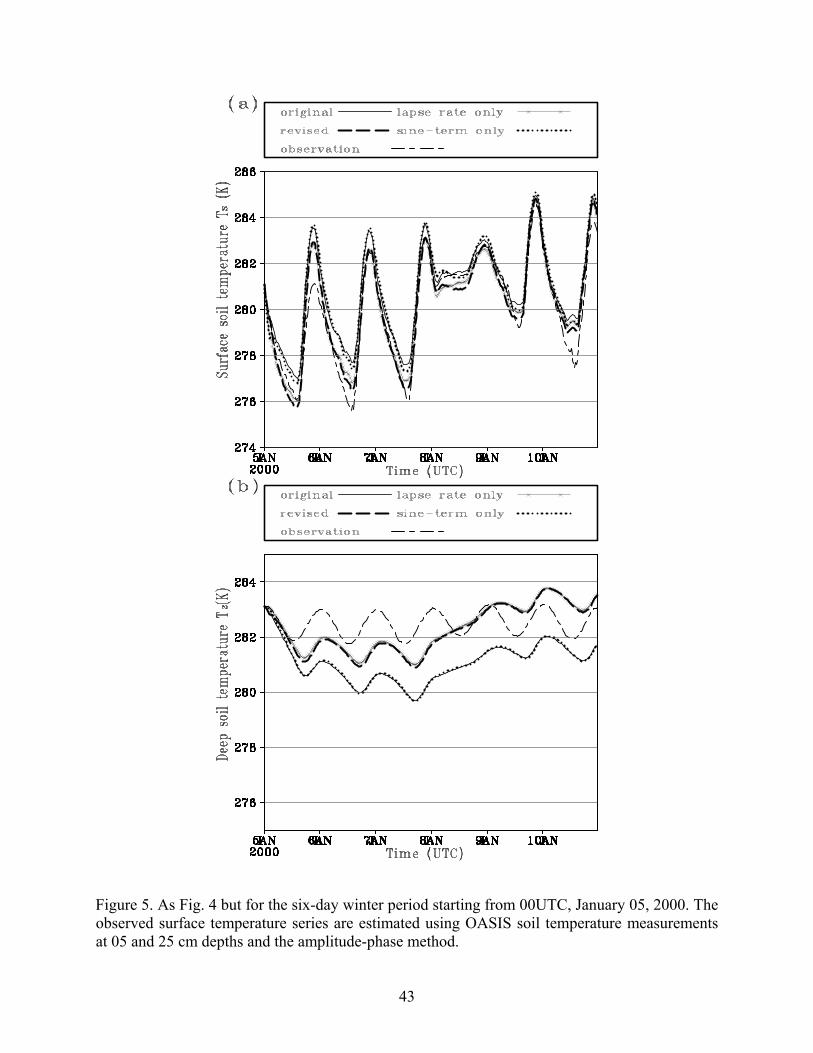
The results from the six-day winter period starting from 00UTC 5 January 2000 are

presented in Fig. 5. As pointed out earlier, the observed skin temperature in this case is

extrapolated from the soil temperature measured at 5 cm using Eq.(10). In general, the revised

model, or the version that includes the lapse-rate related terms, provides an improved deep soil

temperature forecast (Fig. 5b). In this case, the T2 predicted by the original formulation has a

tendency to drift below the temperature of observed values, opposite in direction to the summer

case. This can again be explained by the fact that the mean lapse rate is neglected in the original

formulation and in winter the mean surface temperature is lower that the mean temperature at the

deeper layer. The original model tends to pull the deep layer temperature towards that of the

surface. The improvement in T2 forecast is not as consistent through the period as in the summer,

however. This can be attributed to the fact that during this period, the surface temperature is not

very periodic from day 4 (8 January 2000). The first three days represent is a clear calm period

after a cold front passage, whereas the last two days is a warming up period. For day four, the

observed shortwave solar radiation fluxes reaching the ground clearly indicate cloudy sky

conditions and the daily maximum downward longwave radiation shows a 30% increase that

prevented surface temperature from decreasing as much at night. The aperiodic behavior in the

22

skin temperature leads to poorer prediction of both skin and deep layer temperatures from day

four to day five.

In contrast to the selected summer period, the daytime forcing is milder in the winter.

Also, soil moisture content is larger due to several antecedent rainfall events (with the most

recent one occurring on 03 January). Estimated using the soil moisture content at 5 cm, the

volumetric soil heat capacity of this winter period is 2.6 times that of the summer period. This

effect works in accord with the reduced energy balance term and significantly reduces the

relative importance of ( )G netC R LE H− − term in Eq. (33). Using the same error statistics, Table

4 illustrates the effect of our modifications on the surface temperature prediction. The rms error

for surface temperature with revised version is reduced to 0.73 K from 1.06 K. The mean bias

error is also significantly reduced from 0.85 K to 0.34 K. Similar results were found when we

applied the same modifications to another wet period starting from 00UTC 6 April, 2000,

suggesting that our revised formulation also improves the forecast of surface temperature and the

effect is more evident when the primary force term in the equation is weaker.

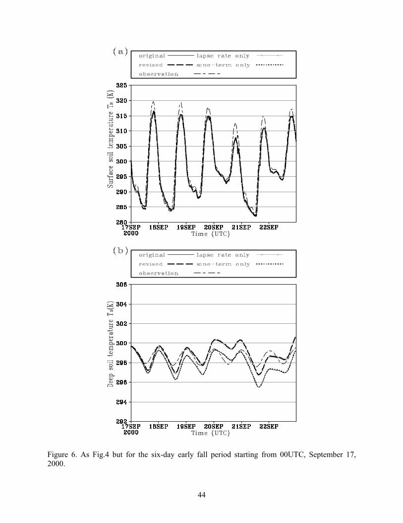
The results from the six-day early fall period starting from September 17, 2000 are shown

in Fig. 6. The daily minimum skin temperature is well predicted, with difference from the

observation being less than 2 K for all the days. The model fails to produce as high day-time

maximum temperatures as observed for all of the days although the difference is generally less

than 5 K except for day four when the maximum skin temperature is significantly lower than the

other days. This abrupt change in the atmospheric forcing must have been contributed to this

larger error since interruption of sinusoidal behavior of surface conditions is expected to increase

errors in force-restore model prediction. The predictions of the deep layer soil temperature using

the revised or lapse-rate-only version of the model is generally better than the original or the

23

sine-term-only case, except for day four (20 September), when surface temperature exhibited

non-sinusoidal behavior (Fig. 6b). The original deep soil temperature curve drifts downward

then oscillates around a level that is about 0.6 K colder than the observed mean deep soil

temperature. After including the lapse-rate related terms, the T2 curve oscillates around a value

closer to the true mean value of the deep soil temperature, giving a much closer fit to the

observations. A more careful look shows that in the first half day, the difference between the

modified and the original version is small, but the difference grows larger with time and reaches

a steady level after a couple of days. This is so because the restore term in the original

formulation acts to drag the deep layer temperature towards the mean surface temperature, which

is about 298.6 K, instead of the seasonally mean temperature of 299.2 K in this case. Again, the

inclusion of the lapse rate terms is most effective in improving the deep soil temperature

prediction and the effect of including the sine-terms is negligible, results consistent with those of

earlier cases.

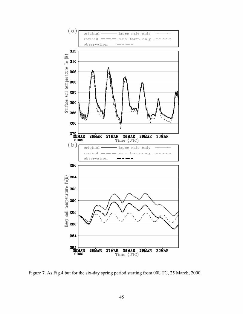
For the spring of 2000, it was hard to find a weeklong period with totally clear sky

conditions at the Norman site. For the 25-31 March period, the first four days generally satisfy

the periodic atmospheric forcing conditions at the surface. At day five, there was a cold front

passage that caused significant daytime temperature drop (Fig. 7a). Our calculation obtains the

average soil temperatures using data from all six days, resulting in a smaller average temperature

difference between the surface and deep layer. This explains at least partly why the deep soil

temperature trend is not totally removed for the first four days of simulation (Fig. 7b) when the

atmospheric forcing is rather periodic. Still, with the inclusion of the lapse rate term, the deep

layer temperature error is reduced by about half (Fig. 7b and Table 3), or 2-3 degrees most of the

time. The improvement in the skin temperature forecast is evident (see Table 3), though not as

24

large. It should be noted that the skin temperature forecast is not bad (rms ≈ 1.5 K and maximum

absolute error ≈ 3 K for the revised model) despite the non-periodic behavior around day four.

To avoid the interference of the cold front passage in the later part of the period, we

repeated the test using data from the first three days only, for which the mean temperature

difference between the surface and the deep layer is 3.5 K instead of the 2 K. In this case, the

revised scheme gives a much improved deep soil temperature forecast (figures not shown). The

difference between the forecast and observations are within 1 K and no apparent phase error is

found. The original formulation has a maximum error of more than 2 K. Note that because the

difference in the e-folding scaling depth in the two cases, T2 is not defined at exactly the same

depth.

The numerical experiments for all four seasons share the commonality that for deep soil

temperature, the most effective factor for improving the original force-restore model is to take

into account of the seasonal-mean temperature lapse rate in the equations. The sine terms are of

minimal significance and can therefore be neglected. The improvement to the skin temperature

by the revised formulation is evident though not as dramatic.

6. Summary and Conclusions

In an attempt to clarify the definition and to improve the forecast of the 'deep layer'

temperature in the soil-temperature force-restore model, we re-derived the equations starting

from the heat transfer equation. Our derivation led to a 'deep layer' temperature, commonly

denoted as T2, that is defined as the soil temperature at depth dπ plus a transient term where d is

the e-folding damping depth of soil temperature diurnal oscillations (c.f. Eq. (30)).

Corresponding to this new definition, the prediction equation for T2, Eq. (31), has the same form

as the commonly used one (e.g., NP79), except for an additional term involving the lapse rate of

25

the 'seasonal-mean' soil temperature and the damping depth d. A term involving the same also

appears in the skin temperature prediction equation, Eq. (33), which also includes a transient

term. The impact on the soil temperature prediction by these additional terms are tested against

OASIS observations for four week long periods selected from out of four different seasons in

2000.

The results from these experiments show clear improvement in the prediction by our

revised formulation of both skin and deep layer temperature, with the improvement in the latter

being much more dramatic. The inclusion of the transient (sine) terms and the lapse-rate related

terms are tested separately. It is found that the most effective modification that improves the

deep soil temperature forecast is the one that takes into account of the seasonal-mean soil

temperature lapse rate. The inclusion of the transient (sine) terms is of minimal impact therefore

the transient terms in both the definition of T2 and the skin temperature equation can be neglected

without much impact, resulting in much cleaner equations. The recommended equations to use

are therefore,

22

1 [ ]sT T T dt

π γτ

∂= − − +

∂, (34)

22( ) ( )s

G net sT C R LE H T T dt

π π γτ

∂= − − − − −

∂. (35)

where

2 ( , )T T d tπ= − . (36)

It was found that without the inclusion of the dπ γ terms, the predicted deep-layer temperature

would drift from observed initial value towards the mean of skin temperature, and such drift was

found to be on the order of 5 K for winter and summer for the Norman site and the drift is of

opposite sign in winter and summer. The inclusion of dπ γ terms virtually removes such a drift.

26

We note here that as hard as we have searched the literature, we did not find a rigorous

derivation of equation like (34) for the prediction of T2. Presenting a clean definition of T2 and its

prediction equation is one of the main contributions of this paper.

For dry conditions and periods with relatively strong daytime heating, our revision does

not impact the skin temperature forecast as much but the improvement becomes more significant

for wetter periods. The value of our revision is further supported by the results of our recent

work in which the improved force-restore model, together with equations for soil moisture, is

used to build an adjoint-based 4DVAR system for retrieving initial conditions of the soil model.

The retrieval of the initial soil temperature and moisture is much better with the revised

formulation.

We note here that it may be argued that if we kept the original formulation of the force-

restore model and definite and initialize T2 as the mean of skin temperature, the drift we

observed should not happen. We have verified that this is true, which is not surprising because of

the (correct) original definition by e.g., D75, of T towards which Ts is restored. The key problem

is that the T2 used here is commonly considered the deep layer temperature (see review in

Introduction) and its value is used in parameterizing vegetation processes that involve deep roots.

For this reason, there is clear value in having available the deep layer temperature. Consensus of

the modeling community is that “the root zone temperature must be included in any skillful

model parameterization" (Roger Pielke Sr., personal communications). This will be especially

relevant when the land surface scheme is used in coupled mode with the atmospheric

components because there will be more feedback from the calculations of heat and moisture

fluxes, including that from evapotranspiration.

27

To use the revised system given by Eqs. (34)-(36), one does need to determine dπγ first.

dπγ is the difference between the 'seasonal mean' skin and deep layer temperature, with the latter

is defined at depth dπ . For NWP applications that range from few hours to a couple of weeks,

these two values can be estimated from data of the proceeding days, given that deep layer soil

moisture, a quantity that affects d most, is slowly varying. The data can be either observed or

model forecast values, with the former being preferred. For longer term applications,

climatological values are suggested. Since the needed values are 'seasonal mean' ones, the use of

climatological values is not as bad as it may sound. Parameter d can be determined by the

amplitude-phase method, as done in this paper.

Finally, we note that even though our numerical tests were performed for Norman site

only, the results should be valid for other sites too because the underlining physics are the same.

Furthermore, the land surface processes should be tested within the integrated land-atmospheric

system. In fact, experiments have been performed within the ARPS in a coupled mode and our

modifications are found to improve the forecast of the overall system as well.

28

Appendix. The amplitude-phase method for determining e-folding damping depth of soil

temperature

Suppose four observations are taken regularly during each day, at 6 hour intervals and at

two different depths, it is straightforward to get the following estimate for soil thermal diffusivity

(Sellers 1965):

22 221 1 3 1 2 1 4 12 1

2 21 2 3 2 2 2 4 2

[ ( ) ( )] [ ( ) ( )]4 ( ) ln[ ( ) ( )] [ ( ) ( )]T

T d T d T d T dd dKT d T d T d T d

πτ

−⎧ ⎫− + −−

= ⎨ ⎬− + −⎩ ⎭

Where d1 and d2 are two different depths, τ is period of daily cycle, i.e., 86400 seconds, 1T , 2T ,

3T and 4T are temperature measurements at 00, 06, 12, and 18UTC, respectively. The e-folding

damping depth can then be calculated according to /Td K τ π= .

This method works better for clear sky conditions. Also, to have a better result, d1 and d2

should be separated as far as possible but all within the damping depth d. Since daily sinusoidal

cannot penetrate beyond 60 cm for normal soils, it is suggested that the two selected depths

should all be limited to within 60 cm depth.

For example, on March 25, 2000, from OASIS measurements at NORM, 5 cm soil

temperatures at 00, 06, 12 and 18 UTC are 292.52, 290.28, 288.61 and 289.90 K, respectively,

and 25 cm soil temperatures at are 288.83, 289.30, 289.08 and 288.40K, respectively. Using the

formula, one obtains KT=7×10-7 m2 s-1. Thus d=13.87 cm, and π d=43.6 cm. Soil temperature

damping depths for the four seasons are obtained by applying this method to each day and then

taking then average.

29

Acknowledgement

This work was supported by DOT-FAA grant NA17RJ1227-01, NSF grants ATM9909007 and

ATM0129892. The authors thank Dr. Jerry Brotzge for making available the OASIS data set and

for very helpful discussions on the related issues.

References

Basara, J. B., 2001: The value of point-scale measurements of soil moisture in planetary

boundary layer simulations, School of Meteorology, University of Oklahoma, 225 pp,

Norman.

Betts, A. K., F. Chen, K. E. Mitchell, and Z. I. Janji, 1997: Assessment of the Land Surface and

Boundary Layer Models in Two Operational Versions of the NCEP Eta Model Using

FIFE Data. Mon. Wea. Rev., 125, 2896-2916.

Bhumralkar, C. M., 1975: Numerical experiments on the computation of ground surface

temperature in an atmospheric general circulation model. J. Appl. Meteor., 14, 1246-

1258.

Blackadar, A. K., 1976: Modeling the nocturnal boundary layer. Prec. Third Symp. Atmos. Turb.,

Diffusion and Air Quality, Boston, Amer. Metero. Soc., 46-49.

Boone, A., V. Masson, T. Meyers, and J. Noilhan, 2000: The influence of the inclusion of soil

freezing on simulations by a Soil–Vegetation–Atmosphere Transfer scheme. J. Appl.

Meteor., 39, 1544–1569.

Bouttier, F., J.-F. Mahfouf, and J. Noilhan, 1993: Sequential assimilation of soil moisture from

low-level atmospheric parameters. Part I: Sensitivity and calibration studies. J. Appl.

Meteor., 32, 1335-1351.

30

Brock, F. V., K. C. Crawford, R. L. Elliott, G. W. Cuperus, S. J. Stadler, H. L. Johnson, and

M.D. Eilts, 1995: The Oklahoma Mesonet: A technical overview. J. Atmos. Oceanic

Tech., 12, 5-19.

Brotzge, J. A., 2000: Closure of the surface energy budget, School of Meteorology, University of

Oklahoma, 208 pp, Norman.

Brotzge, J. A. and D. Weber, 2002: Land-surface scheme validation using the Oklahoma

atmospheric surface-layer instrumentation system (OASIS) and Oklahoma Mesonet data:

Preliminary results. Meteor. Atmos. Phy., 80, 189-206.

Calvet, J.-C., J. Noilhan, and P. Bessemoulin, 1998: Retrieving the root-zone soil moisture from

surface soil moisture or temperature estimates: A feasibility study based on field

measurements. J. Appl. Meteor., 37, 371-386.

Chen, F. and J. Dudhia, 2001: Coupling an Advanced Land Surface-Hydrology Model with the

Penn State-NCAR MM5 Modeling System. Part I: Model Implementation and

Sensitivity. Mon. Wea. Rev., 129, 569.

de Vries, D. A., 1963: Thermal properties of soils. Physics of Plant Environment, Wijk, W. R.

V., Ed., John Wiley & sons, Inc, 210-235.

Deardorff, J. W., 1978: Efficient prediction of ground surface temperature and moisture, with

inclusion of a layer of vegetation. J. Geophys. Res., 83(C4), 1889-1903.

Dickinson, R. E. and A. Henderson-Sellers, 1988: Modelling tropical deforestation: A study of

GCM land-surface parametrizations. Quart. J. Roy. Meteor. Soc., 114, 439-462.

Jacquemin, B. and J. Noilhan, 1990: Sensitivity study and validation of a land surface

parameterization using the HAPEX-MOBILHY data set. Bound.-Layer Meteor., 52, 93-

134.

31

Mahfouf, J. F. and J. Noilhan, 1991: Comparative study of various formulations of evaporation

from bare soil using in situ data. J. Appl. Meteor., 30, 1354-1365.

Mahfouf, J. F., A. O. Manzi, J. Noilhan, H. Giordani, and M. De¥que¥, 1995: The land surface

scheme ISBA within the Me¥te¥o-France climate model ARPEGE. Part I:

Implementation and preliminary results. J. Climate, 8, 2039-2057.

Milly, P. C. D. and K. A. Dunne, 1994: Sensitivity of the global water cycle to the water-holding

capacity of land. J. Climate, 7, 506-526.

Noilhan, J. and S. Planton, 1989: A simple parameterization of land surface processes for

meteorological models. Mon. Wea. Rev., 117, 536-549.

Noilhan, J. and P. Lacarre`re, 1995: GCM grid-scale evaporation from mesoscale modelling. J.

Climate, 8, 206-223.

Noilhan, J. and J.-F. Mahfouf, 1996: The ISBA land surface parameterization scheme. Global

and Planetary Change, 13, 145-159.

Sellers, W. D., 1965: Physical Climatology. University of Chicago Press, 272 pp.

Xue, M., K. K. Droegemeier, and V. Wong, 2000: The Advanced Regional Prediction System

(ARPS) - A multiscale nonhydrostatic atmospheric simulation and prediction tool. Part I:

Model dynamics and verification. Meteor. Atmos. Physics, 75, 161-193.

Xue, M., K. K. Droegemeier, V. Wong, A. Shapiro, and K. Brewster, 1995: ARPS Version 4.0

User's Guide. [Available at http://www.caps.ou.edu/ARPS], 380 pp.

Xue, M., K. K. Droegemeier, V. Wong, A. Shapiro, K. Brewster, F. Carr, D. Weber, Y. Liu, and

D.-H. Wang, 2001: The Advanced Regional Prediction System (ARPS) - A multiscale

nonhydrostatic atmospheric simulation and prediction tool. Part II: Model physics and

applications. Meteor. Atmos. Physics, 76, 143-165.

32

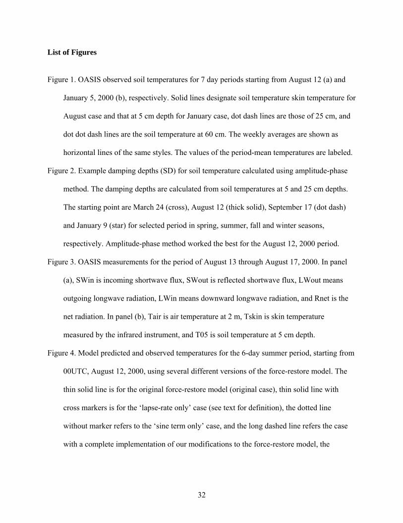
List of Figures

Figure 1. OASIS observed soil temperatures for 7 day periods starting from August 12 (a) and

January 5, 2000 (b), respectively. Solid lines designate soil temperature skin temperature for

August case and that at 5 cm depth for January case, dot dash lines are those of 25 cm, and

dot dot dash lines are the soil temperature at 60 cm. The weekly averages are shown as

horizontal lines of the same styles. The values of the period-mean temperatures are labeled.

Figure 2. Example damping depths (SD) for soil temperature calculated using amplitude-phase

method. The damping depths are calculated from soil temperatures at 5 and 25 cm depths.

The starting point are March 24 (cross), August 12 (thick solid), September 17 (dot dash)

and January 9 (star) for selected period in spring, summer, fall and winter seasons,

respectively. Amplitude-phase method worked the best for the August 12, 2000 period.

Figure 3. OASIS measurements for the period of August 13 through August 17, 2000. In panel

(a), SWin is incoming shortwave flux, SWout is reflected shortwave flux, LWout means

outgoing longwave radiation, LWin means downward longwave radiation, and Rnet is the

net radiation. In panel (b), Tair is air temperature at 2 m, Tskin is skin temperature

measured by the infrared instrument, and T05 is soil temperature at 5 cm depth.

Figure 4. Model predicted and observed temperatures for the 6-day summer period, starting from

00UTC, August 12, 2000, using several different versions of the force-restore model. The

thin solid line is for the original force-restore model (original case), thin solid line with

cross markers is for the ‘lapse-rate only’ case (see text for definition), the dotted line

without marker refers to the ‘sine term only’ case, and the long dashed line refers the case

with a complete implementation of our modifications to the force-restore model, the

33

‘revised’ case. The long-short dash line is for OASIS measurements. Panels (a) and (b)

represent surface and deep soil temperature, respectively.

Figure 5. As Fig. 4 but for the six-day winter period starting from 00UTC, January 05, 2000. The

observed surface temperature series are estimated using OASIS soil temperature

measurements at 05 and 25 cm depths and the amplitude-phase method.

Figure 6. As Fig.4 but for the six-day early fall period starting from 00UTC, September 17,

2000.

Figure 7. As Fig.4 but for the six-day spring period starting from 00UTC, 25 March, 2000.

34

List of Tables

Table 1. General information of Norman super OASIS site

Table 2. Leaf area index (LAI), difference between seasonal mean surface and deep layer temperature ( dπ γ ), observed period-average amplitude of skin temperature (A0) and of deep-layer temperature (Adeep), and damping scale depth (d) in the four study periods

Table 3. Error statistics of T2 predictions for different formulations and periods

Table 4. Error statistics of Ts predictions with different formulations for the winter period

35

Table 1. General information of Norman super OASIS site

Site ID Location (deg) Elevation (m) Slope (deg) Land use Soil type

NORM 35.26N, 97.48W 360.0 0.0 Scrub Silty clay

36

Table 2. Leaf area index (LAI), difference between seasonal mean surface and deep layer temperature ( dπ γ ), observed period-average amplitude of skin temperature (A0) and of

deep-layer temperature (Adeep), and damping scale depth (d) in the four study periods

LAI dπ γ (K) A0 (K) Adeep (K) d (m) Spring (3/25-3/31) 0.22 2.0 9.62 0.74 0.155 Summer (8/12-8/18) 0.60 4.70 15.52 1.34 0.148 Fall (9/17-9/23) 0.50 -0.51 12.50 1.23 0.164 Winter (1/5-1/11) 0.06 -2.17 2.87 0.61 0.146

37

Table 3. Error statistics of T2 predictions for different formulations and periods

Period and mean T2

Formulation

rms (K) Mean Bias Error(K)

Max. Absolute Error (K)

Original 3.3246 3.1323 5.00 Summer Revised 0.6839 -0.3237 1.89

2 301.98T = Lapse rate only 0.7019 -0.3699 1.96 Sine term only 3.3772 3.1866 5.12 Original 1.439 -1.282 2.69

Winter Revised 0.920 0.10 1.58

2 282.52T = Lapse rate only 0.895 0.14 1.57 Sine term only 1.434 -1.268 2.73 Original 1.086 -0.64 3.50

Fall Revised 1.043 0.43 2.60

2 298.59T = Lapse rate only 1.029 0.39 2.59 Sine term only 1.074 -0.60 3.50 Original 2.20 1.739 3.87

Spring Revised 1.54 0.062 3.09

2 286.98T = Lapse rate only 1.55 0.021 3.14 Sine term only 2.24 1.783 3.93

38

Table 4. Error statistics of Ts predictions with different formulations for the winter period

Winter 280.352sT =

rms (K) Mean Bias Error(K)

Max. Absolute Error (K)

Original 1.06 0.85 2.53 Revised 0.73 0.34 2.33

Lapse rate only 0.77 0.36 2.40 Sine term only 1.04 0.84 2.63

39

Figure 1. OASIS observed soil temperatures for 7 day periods starting from August 12 (a) and January 5, 2000 (b), respectively. Solid lines designate soil temperature skin temperature for August case and that at 5 cm depth for January case, dot dash lines are those of 25 cm, and dot dot dash lines are the soil temperature at 60 cm. The weekly averages are shown as horizontal lines of the same styles. The values of the period-mean temperatures are labeled.

40

0

0.1

0.2

0.3

0.4

UTC hours

Scal

ing

dept

h fo

r s

oil t

empe

ratu

re (m

)

SD_sp SD_su SD_fa SD_wt

0 24 48 72

Figure 2. Example damping depths (SD) for soil temperature calculated using amplitude-phase method. The damping depths are calculated from soil temperatures at 5 and 25 cm depths. The starting point are March 24 (cross), August 12 (thick solid), September 17 (dot dash) and January 9 (star) for selected period in spring, summer, fall and winter seasons, respectively. Amplitude-phase method worked the best for the August 12, 2000 period.

41

Figure 3. OASIS measurements for the period of August 13 through August 17, 2000. In panel (a), SWin is incoming shortwave flux, SWout is reflected shortwave flux, LWout means outgoing longwave radiation, LWin means downward longwave radiation, and Rnet is the net radiation. In panel (b), Tair is air temperature at 2 m, Tskin is skin temperature measured by the infrared instrument, and T05 is soil temperature at 5 cm depth.

42

Figure 4. Model predicted and observed temperatures for the 6-day summer period, starting from 00UTC, August 12, 2000, using several different versions of the force-restore model. The thin solid line is for the original force-restore model (original case), thin solid line with cross markers is for the ‘lapse-rate only’ case (see text for definition), the dotted line without marker refers to the ‘sine term only’ case, and the long dashed line refers the case with a complete implementation of our modifications to the force-restore model, the ‘revised’ case. The long-short dash line is for OASIS measurements. Panels (a) and (b) represent surface and deep soil temperature, respectively.

43

Figure 5. As Fig. 4 but for the six-day winter period starting from 00UTC, January 05, 2000. The observed surface temperature series are estimated using OASIS soil temperature measurements at 05 and 25 cm depths and the amplitude-phase method.

44

Figure 6. As Fig.4 but for the six-day early fall period starting from 00UTC, September 17, 2000.

45

Figure 7. As Fig.4 but for the six-day spring period starting from 00UTC, 25 March, 2000.