SERI/TR-632-646 UC Categories: 59,62

An Experimental Performance Evaluation of line-Focus Sun Trackers

Randy C. Gee

May 1982

Prepared Under Task No. 1007.99 WPA No. 05-279

Solar Energy Research Institute A Division of Midwest Research Institute

1617 Cole Boulevard Golden, Colorado 80401

Prepared for the U.S. Department of Energy Contract No. EG-77 -C-01-4042

Printed in the United States of America Available from: National Technical Information Service U.S. Department of Commerce 5285 Port Royal Road Springfield, VA 22161 Price:

Microfiche $3.00 Printed Copy $ 5 . 25

NOTICE

This report was prepared as an account of work sponsored by the United States Govern­ment. Neither the United States nor the United States Department of Energy, nor any of their employees, ncr any of their contractors, subcontractors, or their employees, makes any warranty, express or implied, or assumes any legal liability or responsibility for the accuracy, completeness or usefulness of any information, apparatus, product or process disclosed, or represents that its use would not infringe privately owned rights.

TR-646 S=~II_I-------------------

PREFACE

This report provides test data for and an analysis of two line-focus sun trackers. The suppliers of these two sun trackers, Acurex Corp. and Honeywell, Inc., are gratefully acknowledged for their interest and coopera­tion in the project; particularly, Richard Carlton of Acurex Corp. and Marv Schwochert of Honeywell, Inc. The author also thanks Al Lewandowski for pro­viding the test facility space for this project at SERIfs Mid-Temperature Col­lector Research Facility, and C. F. Kutscher, E. K. May, and L. M. Murphy for their review of this report and the improvements they suggested. Finally, thanks go to Robert McNinch for his help in setting up the test equipment during those long, hot summer days.

This work was supported by Jim Rannels, U.S. DOE, as part of the overall tech­nology development effort under the Solar Thermal Program.

Approved for

SOLAR ENERGY RESEARCH INSTITUTE

Thermal Systems and Engineering Branch

ler, Manager Solar ermal and Materials Research

Division

ill

TR-646

S=~II

SUMMARY

Objective: To provide test data for and an analysis of an aperture-based sun tracker and a flux-line sun tracker.

Discussion: Sun trackers are an important component in the operation of line­focus parabolic trough concentrating collectors. Unfortunately, a host of sun tracker problems have plagued many line-focus collector systems, and they established a history of poor performance. Problems have ranged from exces­sive tracker ad;ustment requirements to complete failure to recognize the sun under nonideal sky conditions.

In response to these problems, improvements were made and new sun tracker con­cepts implemented. To provide an accurate evaluation of these sun trackers, an outdoor test stand was built at SERI. Sun trackers were mounted on the stand and tested until their average tracking accuracy as a function of inso­lation level was established. The trackers were tested over a wide range of insolation levels, so that the measured tracking performance would be meaningful to actual operating collector systems.

Most sun trackers fall into two categories: aperture-based and flux-line. Aperture-based trackers sense the sun directly and can be mounted on the para­bolic concentrator. Flux-line trackers have sensors located at or near the receiver and sense the concentrated flux at the focus. One of each type was thoroughly tested, and both trackers performed well during the entire test periods. The tracking problems that were typical of earlier generation sun trackers did not occur. Their tracking performance as a function of insola­tion level was established, and their overall tracking accuracy (rms· error) was calculated.

Conclusions: Both the flux-line tracker and the aperture-based tracker were found to have an effective rms error of about I mrad. This information was then used to determine the impact of the two trackers on the annual energy performance of typical parabolic trough concentrating collectors. One­mrad rms tracking errors were found to result in negligibly small annual per­formance losses. Also, an analysis of the alignment problem for shadow-band sun trackers was performed . The analysis reveals that the difficulties asso­ciated with shadow-band tracker alignment can be a substantial source of tracking error.

v

S=~II_I ____________________ --=T.::.:..R-....::.6....:..-=--46

TABLE OF CONTENTS

1.0 Introduction......................................................... 1

2.0 Sun Trackers: An Overview .......................................... . 3

2.1 Types of Sun Trackers............................................ 3 2.2 Descriptions of Sun Trackers..................................... 6

3.0 Test Method and Results.

3.1 3.2 3.3

Test Method ••.•••.•••••••.• Apparatus .••.••••••••••••.• Results ................................... eo ••••••••••••••••••••••

4.0 Accuracy Analysis •.•.•••••...•..••

4.1 4.2 4.3

Sun Tracker Accuracy Analysis •.•• Annual Performance Analysis •••••. Misalignment Analysis •.••••.••.••

11

11 12 19

21

21 23 26

5.0 Conclusions.......................................................... 31

6.0 References........................................................... 35

Appendix A Appendix B Appendix C

Parabolic Trough Sun-Tracking Angles .•••••••••••••••••••••••• Sun Position Algorithm ••••••..••.•••.••.••••.••••••••••••.•• Parabolic Trough Annual Performance Model .••••••••••••.••••••

vii

37 49 51

S=~II~ ~'I ________________________ T:::.!R:::.--.,.:;:.6..:...46:::....

LIST OF FIGURES

2-1 Computer Tracker.................................................... 3

2-2 Aperture-Based Tracker (Shadow Band Shown).......................... 4

2-3 Flux-Line Tracker................................................... 5

2-4 Acurex Shadow-Band Sensor........................................... 7

2-5 Honeywell Flux-Line Sensor.......................................... 8

2-6 Marshall Space Flight Center Shadow-Band Sensor..................... 8

2-7 Solar Kinetics Shadow-Band Sensor................................... 9

3-1 Sun Tracker Tes t Stand.............................................. 13

3-2 Sun Tracker Sensors Mounted to Test Collector ....................... 13

3-3 Hydraulic Drive Rotary Actuator Mounted to Test Collector ........... 13

3-4 Hydraulic Drive Power and Control Unit .............................. 13

3-5 Incremental Shaft Encoder ........................................... 14

3-6 Computer Printout of Test Data...................................... 15

3-7 Sample Test Data Shown Graphically.................................. 16

3-8 Adjusted Test Data Sample........................................... 18

3-9 Sun Tracker RMS Error vs. Direct Normal Irradiance for Shadow-Band Tracker. . . . . . . . . . . . . . . . . . . . . . . . . . . . . . . . . . . . . . . . . . . . . . . . . . . . . . . . . . . 19

3-10 Sun Tracker RMS Error vs. Direct Normal Irradiance for Flux-Line Tracker. . . . . . . . . . . . . . . . . . . . . . . . . . . . . . . . . . . . . . . . . . . . . . . . . . . . . . . . . . . 20

4-1 Effective Annual RMS Error of a Shadow-Band Tracker for Several U .8. Cities ........................................ ~.............. 22

4-2 Effective Annual RMS Error of a Flux-Line Tracker for Several U.S. Cities....................................................... 23

4-3 Intercept Factor Y vs. 0totalC for Different Rim Angles for a Cylindrical Receiver.............................................. 25

4-4 Annual Tracking Error Energy Losses vs. P~S Sun-Tracking Error ...... 26

4-5 Shadow-Band Misalignment Schematic.................................. 27

ix

S=~II*I ____________________ --=T:.::.:.R--..::6~46

LIST OF FIGURES (Concluded)

4-6 Misalignment-Induced Tracking Error for East-West Rotational-Axis Parabolic Troughs................................................. 28

4-7 Misalignment-Induced Tracking Error for North-South Rotational-Axis Parabolic Troughs................................................. 29

A-I Parabolic Trough Reference Frame.................................... 37

A-2 Alignment of Parabolic Trough with Sun Vector ....................... 38

A-3 Sun Vector Component in Inertial Reference Frame .................... 39

A-4 Rotation of Parabolic Trough Tracking Axis Away from Local East •.•.. 40

A-5 Rotation of Parabolic Trough Tracking Axis Away from Horizontal ...•. 41

A-6 Rotation of Parabolic Trough to Correct Tracking Angle .............. 42

A-7 Shadow-Band Misalignment Schematic .................................. 45

A-8 Rotation of Parabolic Trough to Tracking Angle for Misaligned Shadow-Band Sensor................................................ 46

x

S=~I TR-646

SECTION 1.0

INTRODUCTION

Sun trackers are sensing elements used to orient the position of a solar col­lector toward the sun. Parabolic troughs must accurately follow the apparent movement of the sun during the day, in one axis, to maintain the receiver at the focus of the concentrator. Tracking errors result in a larger and mis­directed flux concentration at the receiver, which reduces the amount of energy intercepted by it. Therefore, if sun trackers do not position the con­centrator accurately in the correct direction, the collector's performance is significantly and adversely affected.

The tracking performance of many concentrating collector systems has been poor. For example, the tracking system for the parabolic troughs at the Gila­Bend irrigation pumping system required more maintenance time than any other single component of the system [1). The most notable problem at Gila-Bend and other installations [2) has been a drop-off in performance caused by variable sky conditions and insolation levels. Manufacturers who attended a 1977 con­centrating collector conference identified three areas where improvements were most needed; one of them was sun trackers [3). In some cases, sun trackers have tracked passing clouds rather than the sun. In other installations, sun tracker electronics have been sensitive over only a narrow band of insolation levels. l,fuen the insolation level was outside that band, the trackers were unable to distinguish the sun, resulting in large tracking errors. By manually adjusting the sensitivity of the tracker sensors, the functional range of insolation could be shifted and the sun trackers made to work. In some cases, trackers adjusted for a low insolation range (cloudy, hazy sky) became overly sensitive on clear, bright days and drive system cycling (e.g., rapid and repeated clockwise-counterclockwise movements) occurred which could damage the drive system. Therefore, to maintain tracking accuracy over a range of sky, cloud, and insolation conditions, an excessive amount of manual adjustment has been required.

Another common problem has been the difficulty of aligning sun trackers. Adjusting the tracker position to provide a "best focus" on the receiver at one time during the day does not ensure a best focus at other times of the day. The large number of sun tracker alignments that have had to be performed at some parabolic trough installations has been an especially frustrating experience.

Because of these problems, sun trackers have recently been actively developed. Improvements have been made to the sun tracker geometries, more sophisticated electronics have been utilized, arid some new sun tracker con­cepts have been implemented. Most of the improvements were designed to reduce the impact that diffuse irradiance has on the tracking sensors, so that they are principally influenced by only the direct or beam irradiance.

The degree to which these improvements have resolved sun-tracking problems is not clear. Hence, to provide the data needed to quantify accurately some of these new sun trackers, a sun tracker testing program was implemented. This testing program was designed to provide a quantitative measure of tracking

1

S=~I TR-646

accuracy under a wide range of insolation levels and sky/cloud conditions. The measure selected to describe each tracker's performance was its root-mean­square tracking error, Gtrack. Thus, it was necessary to consider a tracker's performance over an extended period of time. By monitoring sun-tracker pointing errors over a certain time span, a frequency distribution of tracking errors can be determined. Such a distribution can then be used to calculate a rms tracking error Gtrack that can be accounted for analytically in a parabolic trough performance analysis.

Tracking errors induced by sun tracker misalignment are also considered. The tracking errors that result from sun tracker misalignment are solved for ana­lytically, given the angular misalignment of the sun tracker head. The magni­tude of these misalignment-induced tracking errors is shown to be quite sub­stantial. Thus, unless aperture-based sun tracker alignment is done with great accuracy, resulting tracking errors can be quite significant.

:2

S=~II~ : TR-646

SECTION 2.0

SUN TRACKERS: AN OVERVIEW

2.1 TYPES OF SUN TRACKERS

There are three major types of sun trackers: computer trackers, aperture­based trackers, and flux-line trackers. A computer tracker (see Fig. 2-1) uses a clock input to compute the sun's position and initiates collector rotation to this computed angle. Although quite simple in theory, this type of tracker requires an accurate method of determining the collector's ahgular position as it is rotated. An angular position device with sufficient resolution to permit accurate tracking is quite expensive. The most commonly used device of this type is an optical shaft encoder. However, because high­resolution optical shaft encoders are expensive, computer tracking is not widely used.

The other two tracking methods, aperture-based tracking (see Fig. 2-2) and flux-line tracking (Fig. 2-3) utilize a simple feedback loop to track the sun. An error signal is generated by the sun-tracker sensor if the collector is not correctly pointed at the sun. When the error signal exceeds a thres­hold, the collector drive system initiates collector rotation until the tracker electronics are once again satisfied. Aperture-based trackers and flux-line trackers differ principally in where the sun tracking sensors are located. An aperture-based sun tracker can be mounted anywhere on the col­lector (usually on the concentrator's edge near the center of the collector row) and rotates with it. Flux-line trackers are mounted on or near the receiver of the parabolic trough.

Clock

Collector ~I Error .. Angle Signal

Figure 2-1- Computer Tracker

3

TR-646 S = ..... !,'!'!!II ~~ ~ I~' ----------------------------------------------------------------------------_

Figure 2-2. Aperture-Based Tracker (Shadow Band Shown)

I.

!s=~I/. ' ___________________________________________ T=R~-~64~6

Error Signal

Figure 2-3. Flux-Line Tracker

Collector Drive

o M ;; g

Shadow-band trackers are the most popular of the aperture-based trackers. Two sensors are separated by a partition or shadowing strip, which shades one of the sensors if the tracker is not pointed directly at the sun. The sensors produce an error signal, which is typically a voltage, when both sensors are not equally illuminated. This error signal, which indicates a pointing error, is used to start the collector rotating until it is correctly pointed. The geometry of the shading strip and placement of the sensors vary greatly among manufacturers, but all rely on generation of an error signal that results from unequal illumination by the sun.

The sensors of the flux-line sun trackers, located at or near the receiver, are sensitive to concentrated flux. As with aperture-based trackers, if the collector is mispointed, an error signal is generated which in turn controls the rotation of "the collector.

Each type of sun tracker has its advantages and disadvantages. Aperture-based trackers rely on a fixed relationship between the focal line and the tracking sensor. If the relationship of the sensor changes with respect to the focal line (e.g., because of deformation of the concentrator or sagging of the receiver tube), an aperture-based tracker cannot compensate for that with an adjusted tracking angle. A flux-line tracker can compensate for these effects, at least at the point along the receiver where the flux-line sensor is located, because flux-line trackers actually sense the position of the con­centrated flux relative to the receiver. A disadvantage associated with flux­line trackers is that the tracking angle is set based on only the relatively small concentrator area that the sun sensors are viewing. If this area hap­pens not to be representative of the overall concentrator (e.g., there is localized concentrator deformation or reflector degradation, excessive dirt or

5

TR-646

dust soiling), the majority of the receiver may not be in optimum focus. An aperture-based tracker will not be affected by any such changes in the collec­tor.

Both flux-line requirements. in two planes. of the trough. aperture plane.

and aperture-based trackers have their own unique installation Aperture-based tracker sensors must be very carefully aligned First, they must be aligned parallel with the rotational axis

They must also be aligned perpendicular to the collector's (This sometimes troublesome task is discussed in Sec. 4.3.)

The best location for the sensors on a flux-line tracker depends on the con­centrator and receiver characteristics. Hence, the sensor is adjusted differ­ently for different parabolic trough geometries. After the best sensor adjustment scheme is determined, the sensors for each collector must be adjusted in the same way.

In this discussion of the advantages and disadvantages of flux-line trackers and aperture-based trackers, neither one stands out clearly as superior to the other. Fora well-designed and well-maintained collector with little concen­trator and receiver deformation or degradation, both types of sun trackers are adequate if they are installed and adjusted correctly. The merits of individual sun trackers should, therefore, be judged principally on tracking accuracy, cost, durability, reliability, and control features. In this report, we examine only tracking accuracy.

2.2 DESCRIPTIONS OF SUN TRACKERS

Several organizations have been developing sun trackers and have incorporated improvements over prior designs. These companies include Acurex, Alpha Solarco, Del, Honeywell, Solar Kinetics, and Sunpower. Honeywell manufactures a flux-line tracker; the rest are aperture-based. Marshall Space Flight Cen­ter has also developed an aperture-based sun tracker; and Sandia Laboratories, Albuquerque, is developing several concepts that provide for "flux integra­tion" along the receiver tube [4]. Al though severa I of these trackers were provided to SERI by their manufacturers, only two were thoroughly tested because of limitations of time or of the hydraulic drive system (see Sec. 3.2) on the tracker test stand. A brief description of the trackers provided is given below.

The Acurex shadow-band sensor is shown in Fig. 2-4. The field of view of the sensor is narrower than that of an earlier model to eliminate much of the influence of clouds and diffuse sky radiation. Also, the electronics have been altered to compensate automatically for changing insolation levels. Further, Acurex has added an additional element of control, a direct insola­tion monitor (DIM). The DIM initiates tracking only when direct insolation exceeds a threshold value. Should a cloud pass the sun, the DIM instructs each collector to hold its position. IVhen the sun reappears and a direct insolation threshold is exceeded, normal tracking continues.

6

S=~I TR-646

Figure 2-4. Acurex Shadow-Band Sensor

Alpha Solarco has developed an aperture-based sun tracker that is not a shadow-band type. Their sun tracker consists of a box-like rectangular housing with a small line-focusing concentrator located along the bottom edge and a clear plastic window along the top edge. The clear plastic window has two thermistors near its center but slightly separated. The focal length of the concentrator is equal to the height of the housing, so that when pointed to the sun, the concentrator focus is along the clear window. i-lhen pointed correctly, the thermistors are equally heated and provide a balanced elec­tronic circuit. T-lhen mispointed,.an error signal is generated.

Honeywell has recently completed development of a microprocessor-based flux line tracker. Their tracker senses the concentrated flux near the receiver. Sensors are mounted on either side of the receiver so that when correctly tracking, the sensors straddle the flux line. Figure 2-5 shows the Honeywell flux sensor mounted on a typical receiver. To acquire the sun initially, the collector is rotated until one of the sensors receives concentrated flux. The collector is then rotated in increments until the flux beam balances the sen­sors. If mispointed, the sensors generate an error signal, and the collector is rotated until the sensors again straddle the flux line.

The Marshall Space Flight Center has developed a shadow-band tracker for horth-south rotational-axis collectors that reverts to a clock drive when clouds obscure the sun. Figure 2-6 contains a schematic of the tracker. Silicon cells provide the error signal, which controls the collector's rotation during normal tracking operation. The field of view of the cells is restricted so that they are not subject to sky/cloud conditions away from the sun. When a cloud covers the sun, cell outputs drop and the tracker circuitry is signaled to provide a consistent, but intermittent, tracking rate of 15 degrees per hour. For north-south rotational-axis collectors; this

7

S=~I /. , TR-646 ~ 7

Figure 2-5. Honeywell Flux-Line Sensor

Plastic Cover

Partition

Solar C~lIs

Opaque Coating (Except for Windows)

Black Inside Wall

White Outside Wall

Terminal Posts (for Connections to Cells)

Figure 2-6. Marshall Space Flight Center Shadow-Band Sensor

8

S=~II*J ______________________ ~T!._"'R'__-),,!.;I..64,6

constant drive rate keeps the tracker roughly pointed at the sun, even in cloudy conditions. 1fhen the sun reappears, it is within the acquisition angle of the sensor, and the silicon cells resume control. This tracker will not function correctly with an east-west rotational-axis parabolic trough because of the large variation in tracking rate during the day for this orientation.

Solar Kinetics has also developed a shadow-band sun tracker. It is different from most shadow-band trackers in that its two sensors are not separated by a partition or shadowing strip. Instead, the edges of the surrounding housing are used to produce shadows on the sensors. Alignment of this sun tracker is aided by an adjustment bolt (see Fig. 2-7) which is easy to use and is inde­pendent of the bolts used to fasten the sensor to the collector.

Shadow-Band Sensor

Mounting Bracket

L--__ Edge Extrusion

Figure 2-7. Solar Kinetics Shadow-Band Sensor

9

10

TR-646 S5~1~ :------------------------------------

SECTION 3.0

TEST METHOD AND RESULTS

3.1 TEST METHOD

The accuracy of a sun tracker may be stated in several ways. One often-cited accuracy measure is the angular pointing error required for the sun tracker electronics to initiate collector rotation. However, this maximum pointing error is typically not a constant but varies with the irradiation level. A more meaningful measure of the sun tracker's accuracy is its root-mean-square (rms) angular pointing error over an extended period of time. A tracker's rms tracking error is a measure of tracking accuracy based on the standard sta­tistical method of quantifying the extent to which a normally distributed quantity varies. Therefore, this measure accounts for variations in tracking accuracy as sky conditions change and irradiation levels vary. For a given sample of a tracker's instantaneous tracking errors (denoted as 8track error) the rms tracking error, C5 track' is ca lcula ted as:

C5 =[ i a~raCk error12jl 1/2

track n (3-1)

where n is the total number of instantaneous tracking error data points in the sample.

One way of evaluating C5 track for a given tracker would be to monitor its tracking errors for a very long time--perhaps a year--so that an average vari­ation in irradiation levels is obtained. However, the results of such an approach would be applicable only for climates or sites similar to that of the test location.

A second, more general, way to quantify tracking accuracy is to determine experimentally the impact that different irradiation levels have on tracking error* and use this relationship to determine how the tracker will perform over the long term. Essentially, this involves determining a tracker's accuracy as a function of irradiation level and then using the known long-term average distribution of irradiation levels for a given site to calculate the effective annual' rms pointing error of the sun tracker. This second' method involves a shorter test period and also provides a more accurate represen­tation of the sun tracker's behavior. This method also permits us to deter­mine a tracker's accuracy for sites other than the test location by utilizing the long-term average distribution of irradiation levels for any particular site. The calculation procedure is described in Sec. 4.0.

Because the relationship of tracker accuracy to irradiation level was of prin­cipal interest, data were taken over time periods in which irradiance varied considerably. Then, during processing of the sun tracking error data, the rillS

*The dependence of tracking error on other environmental variables was also investigated, but no measurable dependence was found.

11

TR-646

tracking error was calculated for each of several ranges of irradiance. The irradiance-dependent rms tracking error, denoted as 0track(Ib)' was calculated for all data points during th2 data-trackirzg period with direct normal irra­diance levels between 600 Him and 800 Him. Similarly, ° track (Ib ) values were calculated for irradiance ranges of 200 tc 400 W/m2, 400 to 600 w/m2, and 800 W/m2 on up. In this manner, tracking accuracy was determined as a func­tion of direct normal irradiance.

Each tracker underwent a sensitivity adjustment so that its peak nominal per­formance could be set. Each tracker's senfitivity was s<;l so that, under a clear sky with irradiance between 900 Wlm and 1050 Wlm, the sun tracker ini.tiated collector realignment every 30 seconds. Thus, the rms tricking error for each tracker in the high irradiation range (above 800 Wlm ) was about 0.7 mi lliradian (mrad) (0.04 degree). This served as a baseline during the testing of the sun trackers.

3.2 APPARATUS

To provide the necessary test data, a sun-tracker test stand was constructed at SERI's outdoor Mid-Temperature Collector Research Facility (MTCRF). A Del Manufacturing parabolic trough (minus its drive system and receiver) was used as the test concentrator and was fastened to the test facility's concrete pad (see Fig. 3-1). The Del collector was chosen because of its small size (1.6-m2 aperture) and its high torsional rigidity. Rigidity was particularly important for the tests, to minimize any wind deflections or torsional windup along the trough. The Del collector was modified to accept a hydraulic drive and to permit coupling with a shaft encoder, which provided a measure of the collector's rotational position.

Sun trackers generally consist of a control box, which contains the tracker electronics, and a remote sensor, which senses the relative position of the sun. Several remote sensors are shown mounted to the test collector in Fig. 3-2. The tracker electronics were configured to control a hydraulic drive unit, which provides for rotation of the test collector. The hydraulic drive unit ~.;ras designed to allow adjustment of the rotation rate over a wide range so that many different trackers could be tested on the test stand. A hydraulic rotary actuator (see Fig. 3-3) was coupled to the Del collector and provided the rotary motion. The rotary actuator was engaged by a four-way, solenoid-actuated, directional valve. The rotary actuator drive rate was con­trolled by two pressure and temperature compensating control valves--one for clockwise rotation and one for counterclockwise rotation. The valves, hydrau­lic pO\.;rer unit, and accumulator are shown in Fig. 3-4. Rotation rates as 10\.;r as 20 degrees per minute could be set by the control valve adjustments.

One problem encountered during testing was a slight variation in rotation rate over the short time periods typical of a tracker pointing angle correction. This problem excluded testing of sun trackers that required a highly uniform rotation rate at each correction pulse. Another problem encountered during the testing was the slow rotational dri.ft of the rotary actuator during times in which no rotation was intended. This occurred because of a small leak through one port of the double-piloted check valve. As hydraulic fluid leaked through the valve, the small pressure differential that resulted across the

12

TR-646 !;::~I I~I --------------------------------------------------------------------------

Figure 3-1. Sun Tracker Test Stand

Figure 3-3. Hydraulic Drive Rotary Actuator MOunted to Test Collector

13

Figure 3-2. Sun Tracker Sensors Mounted to Test Collector

Figure 3-4. Hydraulic Drive Power aud Control Unit

TR-646

rotary actuator caused it to drift, A small disk brake was subsequently added to the output shaft of the rotary actuator to ensure a rapid stop and hold of the rotary actuator.

The test stand was alignable in both north-south and east-west directions, although most of the testing was done in a north-south orientation. Alignment was accomplished by orienting the test stand at solar noon (for north-south axis tracking) or when the sun was directly east or west (for east-west axis tracking) •

An incremental optical shaft encoder (BEl Ruggedized Assembly Model 37l0D) provided an accurate measure of the test stand's rotary position. The shaft encoder is shown mounted to the Del collector test stand in Fig. 3-5. The encoder provided 12,700 counts per revolution, which allows an angular resolu­tion to 0.5 mrad (0.03 degrees). As the sun was tracked throughout the day, the optical shaft encoder transmitted electrical pulses to a pulse counter which provided a current position count to an on-site computer. The on-site computer (LSI-l1 minicomputer) periodically scanned the irradiation levels (both direct normal and total horizontal irradiation, as measured by a pyrheliometer and pyranometer , respectively) as well as the current position counter. The current position count was compared with a calculated position to determine instantaneous tracking error. The calculated position was deter­mined by the on-site computer using highly accurate sun position algorithms. All the data were recorded for the entire testing period and then processed to determine the rms tracker accuracy.

Figure 3-6 trackers.

is a sample of actual data taken during testing of one of the Figure 3-7 is a graphical illustration of this small sample of test

Figure 3-5. Incremental Shaft Encoder

14

~ TR-646 !;::~I I~I --------------------------------------------------------------------------

l:i. 2~:5! B~. 00 :I.:L :~:,~~:S Z :i. 0 {< 00 :1.:1. ::.~ ~:) ~: :I. :::.~ .. 0 (.! :1.:1. ~.~;';!:I. 4.00 :1.1 2~S: :1..5 .... 00 1.:1. 2:S!:I.ti.O() :1.:1. 2~5!20,.OO

:I.:L 2~5 t :::.~2 y 00 :1.1 ::.::~~:j~:2lt .... OO :i.:I. ;.:.~~:5:t 26 .. 00 :1.:1. 2;"ji2B,OO 1:1. 2~:5t30"OO

:1.:1. 2~:5::3:::'+OO

:1.:1. 2~:5~:34 .... 00 11 2~:) t 36 .... 00 :1.:1. 2~:5: :'5B + 00 :1.:1. ::'.:"j;40.00 :I.:!. 2~:.:.;; 42 (- 00 :1.:1. 2~.i:44(.OO

11 2~::.;t46 .. 00 :I. 1 :,:.~ ~:.:j t 4 t:$ .... 0 0 :1.1 2~:)!~:50+00

:1.:1. ::.~~:5t~:52 .... 00 :1.:1. 2~~j t ~:54? 00 :1.:1. 2:.'): ;"j6 < 00 l:!. :?~;s: ~:SB .... 00 :1.:1. :1.:1. :1.:1.

() ,.00

4,()() :1.1 2(,): (;'),,00

:1.:1. 2b! B .... OO 1:1. 26~:I.0.;.OO

:1.:1. 2(',::1. ;:.~ ,.O() :1.:1. 2f,: :1.4,00 :1.:1. ?6~::I.6{<OO

:1.:1. ::.:.~(jt:i.B .... ()O

11 26t22,,(,'O :1.:1. ;:'.6; 24,00 :1.1 :,:.~6!2t)+OO

:1.1 2f.)!2B .... OO :I.:l. ;;,::6; 30 .. 00 11 ;.:.:~t.,t3~?~OO

:1.:1. ::.~6 t :·~:'li .:. 00 l:L 26! :3{::. ) O() :t:l. ~.:.~(~,; 3D .... 00 :1.1 ~.:.~f.:,t40vOO

11 ::,::(:)t l +2"OO 11 ~.:.~t.'~: 44., (eO

:1.1 ::.::c): ~:.:.;?.;. 00 :l.l 2fJ ~ ~:.:.;4.~ 00

1:L .. ::. / 0.;. <)<> :L 1 ":;:'7 ~,:.:: ~ 00 11 /;·.;.00 :i.:!. .,:': .I {, .. () ()

:1.1 ~:.::'? n {. ()O

C(:lLC ,. Ei\!CDDEI:;~

fIL.l TI";(lt)EL. lh v 1/ OvO() :i. .::';. v 1:.:.:; 0 .. ()() :i.(:·: .. ;.1·4 0,,00 :l.bv:l.2 0 .. 00 :1.6,:1.:1. O,()()

ll>,()? (),OO

1(:){.04 .. ··0<.14 :J.t:,.;.02 ····0 .. :1.4 :L,~·) .. Ol .. ··0.;.:1.4 1~5 .. 9(? ····0 .. :1.4 1 ~'.'j • 'IB _ .. () • 14 :I.~::jvt:jc) ····0 .... :1.4 :!'~:S .. 94 ~··O .. :I.·4 :I.;"j,')3 ····().:l.4 :I.:.'j,'1:1. ····(),ll)

:1. :.'j,?O .... () , 2B :I.~:5 .. BB ····O .... 2B :I.~~:j+n6 ····0 .... 2U

:i.~5vB:!. .. ··O .. 2B :I.~.:jvBO ····0.;.2D :I. ~:5 " '?B .... () ,.2B :!. ~:;.; '" './'.7 ····0 .. ~,:.~B

:!'~::j ,. '.?~:;; ····0 v 43

:I. ~:.:j ~ 6 ~.y\

:l.~:S (. 67 :I.;'j ,. f.,;,,; :i. ~:S v c'} it :I. ~:;,i .... 1.)2

:l. ~:s " ~:.:j 4 :i. ~::j .:. ~::.; ~,:.~

:I.:.'j ,.43 1:'.';.,.4:1.

.1.:.'5.;. 3~:.:,i

l~:.:i ,. :33

·~·o .. 43 .. ··0 't .t~::~;

····0 .. 43 ····0 ,43 .. ··0 .. 43

.. ··0 + t.)()

····0 .. 60 ····0,.(,:,0 ····o~. 60 .. ··o .. !.)()

····0 ,. ~:5'? · .. ·0.;. :.:.:i?

····o? '?? · .. ·0.:. './")' .. ··0 , .. /./

····0+ /".? .... () .;. / ./

.... <J '" //

····0 " '7')'

· .. ·o? B~::.i

... {', ', ...

INC. BEAM DIFFUSE ANGLE INSOL.. INSOL.. 62.44 667.41 223.5::'. 62.44 6?0.60 225,37 6::'..44 663.:1.6 22B,60 62.44 623.B4 240.00 62.44 5'16.::'.:1. 243.0? 62.44 6:1.::'..:1.5 234.53 6::'.,45 646.:l.l> 225.44 62.45 6BO.:l.7 2:1.B.?B 62.45 6?6.1:1. 2:1.'1,16 62.45 7:1.3.:1.1 21'1,()7 62.45 739.6B ::'.:1.7.26 62.45 ?53.5() 21B,56 62.45 76B.3B 2:1.?3? 62.46 B06.63 2:1.3.3:1. 62.46 B3'1.5B 211.?7 6::'..46 850.2:1. 2:1.5,46 62.46 B55.52 2:1.?64 62.46 B62.?6 222.B'I 62,46 B72.53 222.?9 6::'..4? 8??B4 224.53 62.47 B72,53 22'1.27 62.4? B45.?6 236.76 62.47 ?B3.25 251,04 ~2.4? ?17.36 26:1..02 62.47 6BO.:I.? ::'.5'1.34 62.47 6'15.04 ::'.45.56 62.4ti 734.37 23:1..7:1. 62.48 764.:1.2 224.45 62,4B 7?5.B:I. 224.23

,~};,:,~" 4<.=1 62 ... 4(,;;'

/''', I::·· .. ' C).'::. i' ",t,.::>

Bl(:·;. {. :::.~<)

B:I..::'j .. 20 '?90 v h9 73\,:> .. r:)B 6El".7.61

~::.i ~:5 0 " ~:.) :!. ~:'=';02 v (;':,9

:.:,;.1,:L ,. 1 \.::: "::i 6 ~:s v . .;'} 'i./

~? ~~.i :'3 ... 6 ./ 2 11-9,. :1.:':)

Figure 3-6. Computer Printout of Test Data

15

S=~I

0

(j) Q)

-.25 Q) .... 0> Q) -0 -Q) -.50 > til .... f-.... -.75 Q) -0 0 () c: -1.00 w

11:25

16.25

(j) 16.00 Q)

Q) .... 0> Q) -0

15.75 -:!::: 1= -0 Q) 15.50 -~ ::J ()

Cii 15.25 0

15.00 11:25

TR-646

........... ...............

................ ... ..........

. .......... .

11:25:30

.. .. ..

11 :25:30

' .. ...

11:26

Local Time

.. ...

11:26

... ..

Local Time

. . .

11 :26:30

.. .. ...

11 :26:30

. . . ..

Figure 3-7. Sample Test Data Shown Graphically

16

....

11:27

.. ...

11:27

TR-646 S=~I/. "--------------------------------------

~ .

data. The actual ti.lt angle (labeled "encoder travel") was provided by the optical shaft encoder at discrete time intervals. (Note that the encoder travel column of data begins at zero degrees.) The encoder rotation was always measured with respect to the first data point of the day. Therefore, by definition, the first data point always had a zero tilt angle. Later data points were measured with respect to this first point. The calculated tilt angle was found by the minicomputer at each time point based on the latitude and longitude of the test site, the day of fhe year, the orientation of the test collector's rotational axis, and the local time. The calculated tilt angles were computed relative to vertical. All of these data were recorded for later processing, along with direct normal irradiance, diffuse irradiance, and the incidence angle of beam irradiance upon the collector's aperture for each time point. The algorithms used to define the position of the sun are gi ven in Appendix B. The algorithm that provides for calculation of the tilt angle of the trough is given in Appendix A.

Following all data taking, tracking error calculations were performed. The two records of tilt angles (both actual and calculated) were used to provide the instantaneous tracking error at each time point. The actual tilt angles, as provided by the shaft encoder, were all relative to the position of the shaft encoder at the beginning of the data-taking period. This was so because incremental encoders can provide information only about relative rotation and not about the absolute angular position of the device. However, the calcu­lated tilt angles were all computed with respect to vertical. Thus, there was a unique numerical bias between the two tilt-angle data records, depending on when the data taking began for the day and at what absolute angle the incre­mental encoder count was zeroed out. This numerical bias is calculated as

n

8bias

\' 8 - 8 L actual calculated I

n (3-2)

where the summation is taken for all time points in which the direct normal irradiance exceeds 600 W/m2 . A threshold of 600 W/m2 was used so that cloudy points are not used to determine the numerical bias.

The calculation of 8 bias also removes the effects of any test set-up errors during alignment of shadow-band sensors perpendicular to the plane of the col­lector's aperture. If a one-degree misalignment were present, the value of 8 bias would be automatically adjusted by one degree in the data reduction, so that operator-induced misalignment would not be attributed falsely to the sun tracker. However, if the shadow-band sensor is not aligned parallel to the axis of rotation, another more subtle misalignment occurs. This misalignment results in a time-varying tracking error and is, therefore, not completely accounted for in the calculation of the numerical bias, 8bias ' For this reason, all tested shadow-band sensors were aligned very carefully in this direction. Instead of aligning the outer housing of the shadow-band sensor, the cover was removed, and the device that actually creates the shadow was aligned.

17

TR-646

S=~I

Following calculation of the numerical bias between the actual tilt and the calculated tilt data points, the expression used to find the tracking error at each point is

6 track error = e actual - 6 calculated - 6 bias (3-3)

This expression essentially normalizes the two data records.

Figure 3-8 shows the graphical equivalent of this normalization procedure for the two data records of Fig. 3-7. The calculated tilt data points are shown as a continuous line on this figure. The encoder travel data points have been adjusted by 6 bias so that they provide the least possible average deviation from the calculated tilt data points. Here, 6 bias is 16.15 degrees. This is equivalent, in practice, to having the sun tracker adjusted so that when it corrects the collector's position, it slightly overcorrects. This is the optimum adjustment of the tracker (assuming the overcorrection does not result in cycling of the drive system), because it minimizes the overall tracking error. In practice, the alignment of the tracker may not be adjusted so that each collector rotation is a slight overcorrection. In this case, the rms tracking error will be larger than calculated in this report.

16.25

en 16.00 Q) Q) .... OJ Q) "0 15.75 -~ OJ c « 15.50 :!::

1=

15.25

15.00 11:25

L~j~sted Encoder Travel Data Points

11:25:30

Calculated Tilt Data Points Fall Along This Line

11:26 11 :26:30

Local Time

Figure 3-8. Adjusted Test Data Sample

18

11:27

S=~II_I ___________________ --=-TR;:::..-~64..:....:._6

3.3 RESULTS

Both an aperture-based sun tracker and a flux-line sun tracker were thoroughly tested for tracking accuracy. Data were taken under a variety of sky, cloud, and insolation conditions. As expected, the trackers performed well under clear-sky, high-insolation conditions, but tracking accuracy was found to degrade under nonideal conditions. Tracking accuracy was affected principally by the instantaneous direct normal irradiance. The dependence of tracking error on other environmental variables was also investigated, but no measur­able dependence was found. For example, the effect of the incidence angle of the solar irradiance on tracking accuracy was investigated, but no dependence was found. Also, the ratio of diffuse to direct irradiance was investigated as a parameter that might impact tracker accuracy. However, it was found to provide a tracking accuracy correlation that was less precise than that found using only direct normal irradiance. Thus, only the dependence of tracking accuracy on direct normal irradiance is discussed in this section.

A compilation of the test results is shown in Fig. 3-9 for the Acurex shadow­band tracker and in Fig. 3-10 for the Honeywell flux-line tracker. Each data point represents the rms tracking error (calculated as shown in Eq. 3-1), over the irradiance range 'denoted by the bracket, for a day's worth of data. Therefore, each data point plotted represents the computed rms value of many (typically several hundred) instantaneous tracking error data points. The accuracy of both trackers decreased as direct normal irradiance decreased.

1100

1,-"

<0 00 <0

is 1000 0

900 -'" E 800 ---- } ...... ~ 700 Q) () c

600 co

l· "0 co "- 500 '" "-

co 400 E "-0 z 300 } ... -() Q) 200

-- --- -~~::f~r:::ce =215 W/m2 "-

is 100

0 a .05 .10 .15 .20 .25

O'track (lbL RMS Tracking Error (degrees)

Figure 3-9. Sun Tracker RMS Error vs. Direct Normal Irradiance for Shadow-Band Tracker

19

S=~II*I ______________________ T_R-_6_46

1100

1····

r--<Xl :g

1000 8

- 900 N

E ....... 800 ~ }-... Q) 700 () c: .~

600 "0 l-.. ell lo-lo-

(ij 500

E 400 lo-

0

-----l'" '-~U~; I:a~i;n~e - 200 W/m'

z - 300 () Q) .... is 200

100

0 0 .05 .10 .15 .20 .25

O"track (I b), RMS Tracking Error (degrees)

Figure 3-10. Sun Tracker RMS Error vs. Direct Normal Irradiance for Flux-Line Tracker

The basel~ne rms tracking error for both sun trackers at high irradiance (> 800 W/m ) of about 0.04 degrees increases to about 0.10 degrees in the low irradiance range.

The cut:rff irradiance is shown to be 200 W/m2 for the flux-line tracker and 215 W/m- for the shadow-band tracker. Cutoff irradiance is that direct normal irradiance below which the tracker does not track the sun. The cutoff values are average values based on observations made during the tests. Cutoff irra­diance is adjustable to some degree with both trackers, but it was adjusted by each manufacturer to a nominal setting. The two data points well to the right of the others in Fig. 3-9 were not used in analyzing the tracker's perfor­mance. The departure of these two data points from the balance of the data was the result of a concentration of irradiance values between 200 W/m2 and 215 W /m2 on those tw~ days. With this unlikely concentration of irradiance values above 200 W/m but below the cutoff irradiance, the tracker was not tracking much of the time, and large tracking errors were calculated.

20

S=~II TR-646

SECTION 4.0

ACCURACY ANALYSIS

4.1 SUN TRACKER ACCURACY ANALYSIS

Figures 3-9 and 3-10 illustrated the effect that direct normal irradiance has on a sun tracker's accuracy. This functional dependence has been curve-fit, and the polynomial expressions for rms tracking error are given below.

• Tracker l--Shadow-band:

(4-1)

where (J track(Ib) is the rms tracking error in degrees and Ib is direct normal irradiance in W/m2.

Expressing (Jtrack(Ib) in mrad:

(Jtrack(Ib) = 3.0 - 5.20 x 10-3(Ib) + 3.077 x 10-6(Ib)2 .

• Tracker 2--Flux-line:

for (Jtrack(Ib) in degrees, and

(Jtrack(Ib) = 3.7 - 6.98 x 10-3(Ib) + 3.983 x 10-6(Ib)2

(4-2)

(4-3)

(4-4)

Having described tracking accuracy as a function of direct normal irradiance, it is possible to use this functional relationship to compute one unique value of rms error for the tracker. This single value of rms tracking error should be an effective value based on the accuracy of the tracker over an average year. Therefore, this effective value should be related to the distribution of direct normal irradiation during a typical year.

Consider the four rms tracking error values corresponding to the four irra­diance ranges of Figs. 3-9 and 3-10. By weighting each of the rms values by the fractional amount of average annual irradiance within its irradiation band, we obtain an average value of rms tracking error. Similarly, the weighting can be based not on the distribution of direct normal irradiation but on the distribution of irradiation incident on the aperture of a single­axis concentrating collector. This provides a weighting based on a quantity that is closely proportional to energy collection and results in an effective annual rms tracking error. The effective value accounts for the fact that a tracker's accuracy is most important when a large amount of energy is avail­able to the collector. Therefore, a cosine term is included that accounts for the reduction in beam irradiance caused by its incidence angle. Thus, a tracker's effective annual rms tracking error is expressed as

21

!s=~I/. · __________________________________________ ~T~R~-6=4~6 ~ ~

° track JOtrack(Ib) • Ib • cos(S) • dIb

JIb • cos(S) • dIb (4-5)

where the integrals are evaluated over an entire year whenever the cutoff irradiance is exceeded.

This expression for effective rms tracking error has been evaluated numer­ically for both north-south and east-west rotational-axis parabolic troughs. The results for several u.s. cities are shown in Fig. 4-1 for the shadow-band tracker and in Fig. 4-2 for the flux-line tracker. This evaluation is based upon the direct normal irradiation and incident angle distributions for each of the cities as calculated from Typical Meteorological Year (TMY) weather tapes. Note that the effective rms tracking error depends on the average annual direct normal irradiation for the site. This result occurs because of the higher average irradiance and resulting higher tracking accuracies for locations with higher annual average direct normal irradiation. Hence, as Figs. 4-1 and 4-2 indicate, a given sun tracker's average performance will be better over the long term at a high-irradiation ;ocation than at a low­irradiation location. A cutoff irradiance of 200 W/m has been designated the lower limit of integration for Eq. 4-5, since this is the approximate cutoff irradiance for both trackers.

'" - .065 '" (f) "' Q) g Q) 0

"-OJ Q)

~ "-

.060 0 "-"- 0 LU OJ c: 0 ED

.:.:: 0 o North-South Rotational Axis (.)

.055 • East-West Rotational Axis co • 0 "-I- • 0 0 C/)

" ~ • a:: (tj • 0

::J .050 CIties Shown 0 0 c: • c: EI Paso, TX (far right) « Albuquerque, NM • • Q) Dodge City, KS > Fort Worth, TX :;:; (.) .045 Omaha, NE Q) Great Falls, MT -- Brownsville, TX LU

Lake Charles, LA "" Caribou, ME " g New York, NY (far left)

t)

.040 4 5 6 7 8 9 10

Annual Direct Normal Irradiation (GJ/m2)

Figure 4-1. Effective Annual RMS Error of a Shadow-Band Tracker for Several U.S. Gities

22

S=~II_I ______________________ T_R_-6..:...-4-'-6

_ .065 en Cl> Cl> ..... 0) Cl> -0 -o .060 ..... ..... UJ 0) C

.:::t:. (.) C\l ..... I­Cf)

~ a: CO ::l C C « Cl> .~ -(.) Cl> --UJ

.055

.050

.045

o

o • o

• 00

Cities Shown EI Paso, TX (far right) Albuquerque, NM Dodge City, KS Fort Worth, TX Omaha, NE Great Falls, MT Brownsville, TX Lake Charles, LA Caribou, ME

• 0

• •

New York, NY (far left)

o

o North-South Rotational Axis • East-West Rotational Axis

o 0

••

tl .040.J--__ --'-___ -'-___ -'-___ ..I..-__ ---lL.-__ ........

4 5 6 7 8 9 10

Annual Direct Normal Irradiation (GJ/m2)

Figure 4-2. Effective Annual RMS Error of a Flux-Line Tracker for Several U.S. Cities

The dependence of effective rms tracking error on tracking axis direction is small. North-south rotational-axis troughs are shown to result in slightly higher rms tracking errors than east-west rotational-axis troughs. This minor dependence is the result of differences in incidence angles between the two orientations. Cosine losses are significant only away from solar noon for east-west troughs--when direct normal irradiance levels are decreasing. Thus, the tracker's performance typically falls off when the potential for energy collection is also relatively small, and the resulting penalty is small as well. For north-south axis troughs, incidence angles can be high at noon and are at a minimum away from noon. Because peak tracker performance does not typically coincide with peak direct normal irradiance during the day, its annual effective rms tracking error is higher.

Both sun trackers proved to have nearly identical effective rms tracking errors. An effective rms tracking error of 1 mrad (0.057 degrees) is a good average value for both trackers.

4.2 ANNUAL PERFORMANCE ANALYSIS

The previous section described sun tracker accuracy on an average instan­taneous basis. The instantaneous data were then analyzed in terms of an annual rms tracking error. While this information is useful in gaining an understanding of sun tracker performance, it can also be used to quantify the

23

S=~I I: ' ______________________ ---::..TR::..:..--=6...:...46=_

impact that trackers have on the energy collection of parabolic troughs. A method for evaluating a sun tracker's performance in terms of long-term average energy collection is described in this section.

It is useful to consider sun tracking errors over an extended length of time rather than on an instantaneous basis. Over this length of time, a frequency distribution of tracking errors is defined. This distribution can be char­acterized by its rms. value. As shown by Rabl et al. [5], this rms tracking error value can be added quadratically to the other optical error terms to obtain an effective rms optical error, 0optical'

O~Ptical 40~ontour + O~pecular + A(40~ontour + O~pecular)

(4-6)

with

for a concentrator with a 900 rim angle.

The total rms optical error, including the angular beam spread caused by the sun itself, is then calculated as:

°total = (O~ptical + 02 )1/2 sun (4-7)

where ° is the rms angular width of the sun as viewed at the receiver. The sun value of 0sun depends on the incidence angle ei of the sun's irradiation.

0sun = 0sun e. = 0/COS2ei (4-8) , 1

The sun's rms width at an incidence angle of zero degrees is taken to be 2.8 mrad. Rabl et al. note that these equations hold regardless of the individual error distributions; in particular, they do not have to be Gaussian (standard normal) distributions.

The central limit theorem of statistics [6] implies that the distribution resulting from the convolution of a number of independent distributions can be expected to be nearly Gaussian even if the individual components are not Gaussian and if the final distribution is not dominated by a single non­Gaussian component. Thus, while the tracker test data showed the tracking error distributions to be more uniform (i. e., flatter) than Gaussian distri­butions, their quadratic addition with the other optical error distributions is still a good statistical approximation. Further, the fact that the magni­tude of a tracker's rms error is typically small relative to the other terms in the preceding equation indicates that their addition quadratically is appropriate.

The impact that the effective total of all the optical errors has on the optical performance of ~ parabolic trough is shown in Fig. 4-3. The intercept factor of a cylindrical line-focus receiver is shown as a function of the pro­duct o(IJtotal and C (geometric concentration ratio) for a variety of concen-

24

S=~I TR-646

trator rim angles. The intercept factor is defined as the fraction of irra­diation incident on the trough's aperture that reaches the absorber tube of the receiver. Note that increased tracking errors will increase a total' decrease the intercept factor, and thereby decrease the collection efficiency of the parabolic trough. It is clear from Eq. 4-6 that the impact of the tracking error can be evaluated only in conjunction with the other optical characteristics of the collector. Note, however that the dominant optical error is likely to be acontour' the rms concentrator contour (or slope) error, because of its 4 x weighting. Because the contour error is important and because its rms value can vary substantially from one design to another it is best to consider its impact parametrically. The two remaining optical errors, as ecular and a disp ' have been assigned typical values of 1.6 mrad and 2.8 mrad, respectively, and a parabolic trough annual performance model was utilized to predict the impact that the rms tracking error has on annual trough energy collection. The model evaluates how the optical efficiency of a trough· is affected by variations in a track (using Eq. 4-6 and Fig. 4-3) and then uses this information to calculate how the overall collector efficiency is affected. The parabolic trough performance model is described in Appendix C.

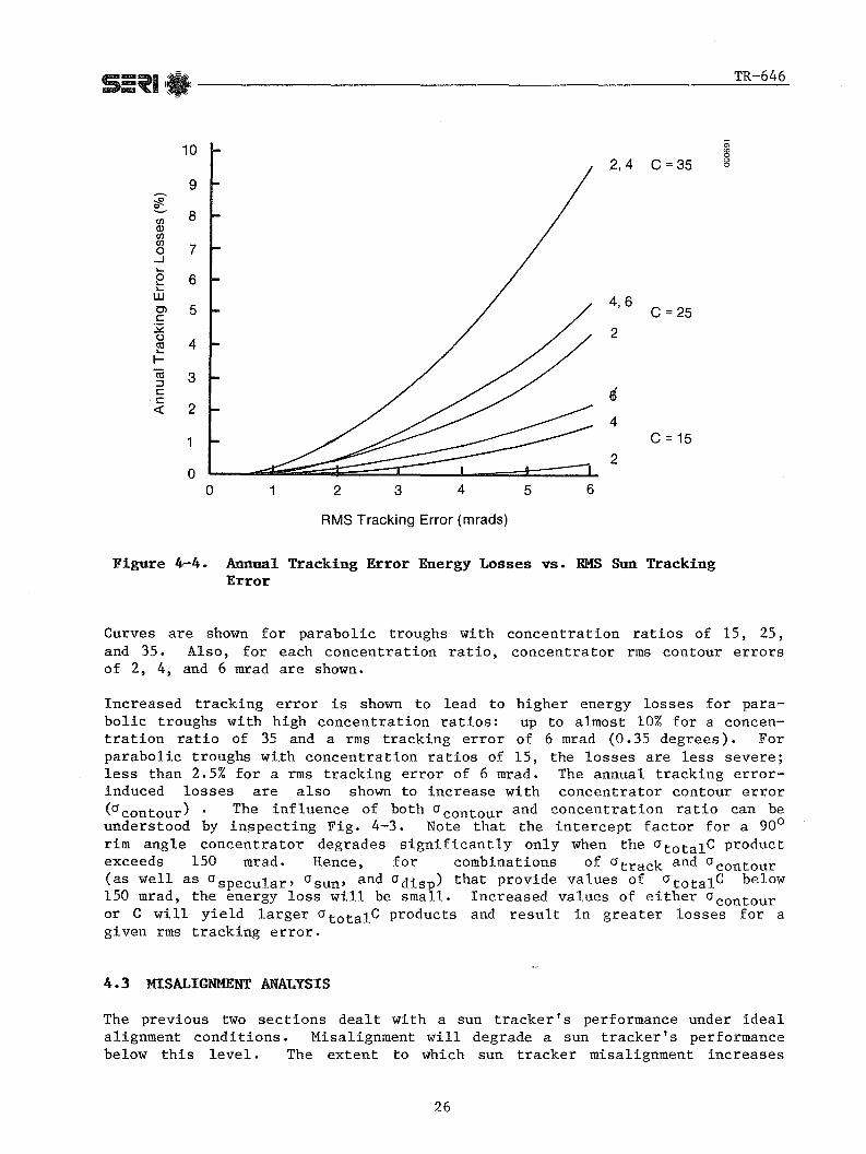
The results of this annual analysis are shown in Fig. 4-4. The percentage of parabolic trough annual energy collection that is lost because of tracking errors is shown as a function of atrack' the effective rms tracking error.

1.0

0.8

0.6

0.4

0.2

o o 100 200 300 400 500

(T tot C (mrad)

Figure 4-3. Intercept Factor Y vs. 0totalC for Different Rim Angles for a Cylindrical Receiver

25

S=~I /. ~I _________________________ TR_-_6_4_6 ~ ~

10

9 ~ ~ 8 (/J Q) (/J (/J

7 0 .....J "-0 6 "-"-w Ol 5 c: 32 ()

4 CI:l "-r "iii 3 ::l c: c:

2 «

1

0 0 1 2 3 4 5 6

RMS Tracking Error (mrads)

2,4 C = 35

4,6

2

e 4

2

C =25

C = 15

Figure 4-4. Annual Tracking Error Energy Losses vs. BMS Sun Tracking Error

Curves are shown for parabolic troughs with concentration ratios of 15, 25, and 35. Also, for each concentration ratio, concentrator rms contour errors of 2, 4, and 6 mrad are shown.

Increased tracking error is shown to lead to higher energy losses for para­bolic troughs with high concentration ratios: up to almost 10% for a concen­tration ratio of 35 and a rms tracking error of 6 mrad (0.35 degrees). For parabolic troughs with concentration ratios of 15, the losses are less severe; less than 2.5% for a rms tracking error of 6 mrad. The annual tracking error­induced losses are also shown to increase with concentrator contour error (cr contour). The influence of both cr contour and concentration ratio can be understood by in$pecting Fig. 4-3. Note that the intercept factor for a 900

rim angle concentrator degrades significantly only when the cr total C product exceeds 150 mrad. Hence, for combinations of crtrack and crcontour (as well as crspecular' cr sun ' and crdisp) that provide values of crtotalC below 150 mrad, the energy loss will be small. Increased values of either crcontour or C will yield larger cr total C products and result in greater losses for a given rms tracking error.

4.3 MISALIGNMENT ANALYSIS

The previous two sections dealt with a sun tracker I s performance under ideal alignment conditions. Misalignment will degrade a sun tracker I s performance below this level. The extent to which sun tracker misalignment increases

26

TR-646

tracking errors depends upon the extent of the misalignment and the direction in which misalignment has occurred.

Figure 4-5 shows a typical shadow-band tracker and identifies the three axes about which ~angular misalignment can occur. Minor rotational misalignments about the UCP-axis have no effect on tracking error. Rotations of this kind simply alter the acceptance angle of irradiation into the tracker head. As long as these rotations are small enough to permit acceptance of irradiation directly from the sun during all times of the year (as the sun's declination chan~) no sun-tracking errors will result. Tracker alignment about the UCA-axis, so that the tracking head is perpendicular to the collector's aperture, is generally accomplished by adjusting the tracker head while the collector is tracking until a "best focus" is obtained on the receiver tube. This alignment is the most critical and is usually performed with relative ease, because it is quite convenient to view the receiver while adjusting for a "best focus." However, a third angular misalignment can occur that invali­date~the "best focus" alignment procedure. This misalignment occurs about the UCN-axis. Ideally, the tracker should be adjusted so that the shadow band is aligned parallel to the collector's rotational axis. This is sometimes set by sighting along the shadow band using the receiver tube or an edge of the concentrator as a reference. Another common practice is to level the shadow band once the collector has been tilted to the horizon. While this works reasonably well if the collector's rotational axis is horizontal, such a pro­cedure is more difficult and less accurate if the rotational axis is not pre­cisely horizontal.

Figure 4-5. Shadow-Band Misalignment Schematic

27

'" '" §

S=~II*I ________________________ T_R_-6_4~6

-~ Whil~misalignment about the UCN-axis is less severe than misalignment about the UCA-axis, it is more difficult to eliminate. Further, its effect on tracking accuracy is more subtle and has been the source of considerable frustration during opera~ion of some concentrating collectors. A symptom of misalignment about the UCN-axis is correct tracking during one part of the day (as evidenced by the "best focus" on the receiver) but incorrect tracking during another part of the day. This phenomenon is i1.lustrated in Figs. 4-6 and 4-7 for selected days of the year, assuming a UCN-axis misalignment of 0.25 degrees* (4 mrad). Note that the behavior of east-west parabolic troughs is significantly different from that of north-south troughs. FOJ both orientations, the tracking angle error that occurs as a result of UCN-axis misalignment approaches zero as the incidence angle of solar irradiation on the tracker approaches zero. Thus, for east-west troughs, the misalignment­induc.ed tracking error is zero only at solar noon. For north-south troughs, the misalignment-induced tracking error is zero only when the sun is due east or west.

en 1.0 Q) Q) ... Lat = 400 Ol Q) Misalignment = .25 0

~ ... 0

.5 ... ... W Ol c

:52 u CIl ... I- 0 -0

12/21 Q) u ::J -0 C .. - -.5 c Q)

E c .2> «i .!!2 ~ -1.0

6 7 8 9 10 11 12 1 2 3 4 5 6

Solar Time

Figure 4-6. Misalignment-Induced Tracking Error for East-West Rotational Axis Parabolic Troughs

*Other UCN-axis misalignments can be easily considered because the resulting tracking error is linearly proportional to misalignment. Thus, a UCN-axis misalignment of 0.5 degrees results in twice the tracking error shown in Figs. 4-6 and 4-7.

28

S=~II_I ____________________ ~T:.::.:;R......:-6:.....:...:..46

en <D 1.0 <D .... en <D '0 -.... o .... ....

LU en c: ~ ()

~ I­'0 <D () ::J '0 c:

.5

o

::c c: -.5 <D E c: en

-1.0

Lat = 400

Misalignment = .250

-~ 6/21

3/21

12/21

6 7 8 9 10 11 12 1 2 3 4 5 6

Solar Time

Figure 4-7. Misalignment-Induced Tracking Error for North-South Rotational­Axis Parabolic Troughs

VariaJions in tracking error according to the time of day are thus symptoms of UCN-axis misalignment. However, this tracking-error variation has some­times no~ been well understood; sun trackers have been adjusted only about their UCA-axis (see Fig. 4-5) to provide a "best focus" at each time of adjustment. However, this provides only an offset or bias to theq. tracking error variations and does not eliminate them. Alignment about the UCN-axis is the proper corrective action. This is often difficult because the sun~!acker heads are not fastened to the collector in away that pe~ts easy UCN-axis adjustment. Until the sun tracker head is aligned in the UCN-axis direction, tracking errors will continue, an~ the frustrations of multiple realignments (if alignment is only along the UCA-axis) will persist.

The alignment of shadow-band sun trackers can be troublesome because the tracker must be aligned in two orthogonal directions, not just one. However, an alignment bracket such as the one utilized by Solar Kinetics greatly aids in the alignment process. That sun tracker alignment bracket is shown in Fig. 2-7. The U-bracket is butted up alongside a reference guide that is known to be precisely parallel to the trough's rotational axis. When the two bolt~that thread into the concentrator ~~e tightened, alignment along the UCN-axis is obtained. Next, to provide UCA-axis alignment, the remaining bolt is adjus~.fd to deform the U-bracket until a "best f~s" is achieved. Because the UCA-axis alignment bolt is independent of the UCN-axis alignment bolts, this procedure is relatively simple and straightforward. It does, however, require that a mounting surface be provided on the collector which is known to be precisely parallel to the trough's rotational axis. While the edge of the concentrator or reflective surface may provide such a guide, the normal angular variations of these surfaces along the length of the trough may

29

S=~I '*1 _______________________ TR_-_6_46

dictate that a more precise reference guide be provided. Because this align­ment is critical to the correct operation of shadow-band trackers, it might be necessary to provide a precisely machined reference guide during fabrication of the trough when the concentrator rotational axis is precisely known. Also, the U-bracket's matching edge should be well machined so that a precise align­ment is possible. Finally, alignment of the edge of this bracket with the edge of the shadow band itself must be ensured. To be safe, this alignment should not be adjustable in the field.

30

TR-646

SECTION 5.0

CONCLUSIONS

From the data and analysis presented in this report, several conclusions can be drawn concerning sun trackers for parabolic trough concentrating col­lectors. Some are specific to the sun trackers tested, and some are general conclusions that apply to all trackers for parabolic trough collectors.

(1) Neither one of the sun trackers tested suffers from. the gross tracking error problems that were typical of early-generation trackers.

The sun trackers that were used on many parabolic trough projects during the 1970s (both privately funded projects and DOE/ERDA demonstration projects) suffered from a variety of problems. The most typical one was an inability to track the sun accurately under a variety of sky and cloud conditions. Diffuse irradiation from areas of the sky away from the sun was often identified as the major source of the tracking diffi­culties; various ways to minimize or eliminate its influence were incorporated into the improved sun trackers. During their entire testing periods, neither sun tracker exhibited any of the gross tracking error characteristics that were typical of early trackers.

(2) Typical parabolic troughs require sun trackers with rms tracking errors of less than 2 to 3 mrad (0.15 degrees) for the resultant optical losses to be negligibly small.

Current state-of-the-art parabolic troughs have geometric concentration ratios near 20 and rms contour errors of 4 to 6 mrad (see Fig. 4-4). With these optical characteristics, the annual sun-tracker-induced losses of a typical trough are less than 1% if the rms tracking error is below 2.5 mrad. For parabolic troughs with lower concentration ratios, the tracking accuracy requirements can be relaxed even more. If parabolic troughs are developed with highly accurate concentrators (contour errors approaching 2 mrad) , higher concentration ratios may be utilized and sun trackers with rms errors below 2 mrad should be employed.

(3) Both of the sun trackers that were thoroughly tested for tracking accuracy were found to have effective rms tracking errors near 1 mrad.

An effective rms tracking error of 1 mrad represents excellent tracking performance and is more than sufficient for typical parabolic trough concentrating collectors. Over the long-term average, a l-mrad rms tracking error permits parabolic trough energy collection within 0.2% of that attainable by a trough with a perfect tracker. Note, however, that these rms values correspond to ideally aligned trackers that are adjusted to initiate collector rotation for approximately every 1/8 degree in sun movement under clear-sky conditions. The effective rms tracking errors of these trackers under more typical adjustment and alignment conditions will be larger.

31

S=~II*I ______________________ ..;:..TR_--:,.6...;.,.:,..46

(4) The tracking accuracies of both the flux-line tracker and the shadoW'­band tracker were found to be affected principally by the instantaneous direct normal irradiance.

The only variable that was found to influence sun tracking accuracy significantly was direct normal irradiance. The rms tracking errors of both trackers increased as the direct irradiance decreased. While the trackers had rms tracking errors of about 0.8 mrad under high levels of direct irradiation (above 800 W/m2), the rms tracking error increased to nearly 2 mrad under low direct irradiation (between 200 W/m2 and 400 W/m2). This relationship indicates that the sun trackers will operate with greater accuracy in locations with higher average irradia­tion. While this is so, the net difference in effective rms tracking error between various locations is very small (see Figs. 4-1 and 4-2).

(5) Both aperture-based and flux-line sun trackers can perform with suf­ficient accuracy for state-of-the-art parabolic trough concentrating collectors; therefore, either tracking concept is valid.

Both types of trackers have individual disadvantages and advantages. Flux-line trackers will compensate for concentrator deformations or receiver sag because they sense the focused light of the flux line and center this flux on the receiver. Aperture-based sun trackers rely on a fixed relationship between the focal line and the tracking sensor and will not compensate for concentrator deformations or receiver sag. How­ever, the fact that aperture-based trackers do not position the concen­trator by means of concentrator optics can also be viewed as an advantage. If concentrator deformation or receiver sag occurs only near the tracking sensor, it would be best not to compensate for them. While the advantages and disadvantages of the two concepts may be debated, trackers of both types have been shown to track sufficiently well for parabolic trough application.

(6) Sun-tracker alignment is a potential source of significant tracking error for aperture-based sun trackers; this concern necessitates that trackers be aligned accurately in two planes.

Aperture-based sun trackers are routinely aligned so that the tracking sensor is perpendicular to the collector's aperture by making adjust­ments until a "best focus" is obtained on the receiver tube. However, the tracker sensor must also be aligned parallel with the rotational axis of the trough. If this is not done accurately, the receiver tube may be in focus during part of the day but out of focus at other times. The resulting optical losses can degrade collector performance severely.

(7) Several manufacturers of aperture-based sun trackers could improve their tracker mounting brackets to make aligning the sun trackers easier and more accurate.

Since aperture-based sun trackers require alignment in two planes, the mounting brackets should permit independent adjustment in both planes. Most mounting brackets do not permit this, however. Also, to aid in aligning the tracker head parallel to the rotational axis of the col­lector, a machined guide should be provided along the concentrator's edge. That would ensure rapid and accurate tracker alignment.

32

S=~I I_I ______________________ -=.::TR:.:.---=..64..:...::,.6

These conclusions are supported by test data for a range of sky, cloud, and irradiation conditions and very favorable mechanical conditions. The hydraulically driven test stand was essentially free of backlash and experienced a minimum amount of wind-induced deformation. The sun trackers were adjusted so that they would correct their angular position approximately every 30 seconds (about 1/8 0 of sun movement) under clear-sky conditions. Sun trackers' performance for a field of parabolic troughs is likely to be degraded below the values reported here, however, if the collectors or drive systems introduce significant mechanical errors, or if the trackers are not aligned optimally. It is also possible, but less likely, that sun trackers' performance in the field may be better than reported if the trackers are made more sensitive and are repositioned more often than every 30 seconds.

Finally, it is important to note that because of the rather short time periods during which each tracker was actually being tested (typically one to two months), no information was gathered on the reliability or durability of the sun trackers. These two factors are perhaps best judged by the quality of the components used in the tracker heads and electronic circuitry as well as by the performance of the unit over extended periods of operation. Other important factors to consider in evaluating or selecting a sun tracker are cost, control features, installation requirements, and associated electrical wiring.

33

34

S=~II*1 ______________________ -=-TR::.!...-...:::6~46

SECTION 6.0

REFERENCES

1. Alexander, G.; et al. Final Report on the Modification and 1978 Oper­ation of the Gila-Bend Solar-Powered Irrigation Pumping System. SAND 79-7009. Albuquerque, NM: Sandia National Laboratories; March 1979.

2.

3.

Gee, R. C.; Kruger, P. D. _=H:.:o:..::n:.:e~yw~e=:::1::..:1=---G=-e::.:n::.e=-r=-a=1-0::.:f:=_:f~i~c-=e.=.s==C_=_o.::n.::c.-=:e.::n:..::t.::r.::a:.:t:.:i::n=.g Collector System--Installation and Operation. 1979 ISES Congress; Atlanta, GA; 28 May-1 June 1979.

"Report of Working Group on Manufacturing." ference on Concentrating Solar Collectors. nology; 26-28 September 1977.

Proceedings of the ERDA Con­Georgia Institute of Tech-

4. Kohler, S. M.; Wilcoxen, J. L. Development of a Microprocessor-Based Sun Tracker System for Solar Collectors. SAND79-2163. Albuquerque, NM: Sandia National Laboratories; April 1980.

5. Rabl, A.; et al. Optical Analysis and Optimization of Line-Focus Solar Collectors. SERI/TR-34-092. Golden, CO: Solar Energy Research Institute; September 1979.

6. Burr, I. W. Applied Statistical Methods. New York, NY: Academic Press; 1974.

7. Duffie, J. A.; Beckman, W. A. Solar Energy Thermal Processes. New York: John Wiley and Sons; 1974.

8. EG&G Final Report lfAG-1407: "A Survey of Tracking Systems and Rotary Joints for Coolant Piping."

9. Almanac for Computers for 1981. Nautical Almanac Office, U.S. Naval Observatory.

10. Duffett-Smith, P. Practical Astronomy. versity Press; 1979.

New York, NY: Cambridge Uni-

11. Collares-Pereira, M.; Rabl, A. "Simple Procedure for Predicting Long­Term Average Performance of Nonconcentrating and Concentrating Solar Col­lectors." Solar Energy. Vol. 23: pp. 235-53; 1979.

12. Harrison, T.; Bond, G.; Ratzel, A. Design Considerations for a Proposed Passive Vacuum Solar Annular Receiver. SAND78-0982. Albuquerque, NM: Sandia National Laboratories; April 1979.

13. Beckman, W. A.; Klein, S. A.; Duffie, J. A. Solar Heating Design by the F-Chart Method. New York: John Wiley and Sons; 1977.

35

55'1 1*1 ______________________ -=TR:;.;;..-...:;,.6-'-=-46

14. Harrison, T. Mid-Temperature Solar Systems Test Facility Predictions for Thermal Performance of the Solar Kinetics T-700 Solar Collector With FEK244 Reflector Surface. SAND80-1964/1. Albuquerque, NM: Sandia National Laboratories; November 1980.

36

S=~II*I ___________________ --=T:..::,:.R--=:6...:...::;.46

APPENDIX A

PARABOLIC TROUGH SUN-TRACKING ANGLES

This appendix describes a solution to the calculation of the collector tilt angle for a single-axis concentrating collector as it tracks the apparent motion of the sun during the day. The solution is given in terms of the sun azimuth and elevation angles and the specific orientation of the single-axis collector. Next, misalignment of an aperture-based sun tracker (mounted to the collector) is introduced and a new solution to the tracking angle is pro­vided. The tracking angle of a parabolic trough is measured from a horizontal plane and was denoted as e calculated in the body of the report. In this appendix, it is denoted as B for conciseness.

Tracking Angle for Single-Axis Collector with Aligned Sun Tracker

Figure A-I shows a typical single-axis parabolic trough concentrating col­lector. It is convenient to define a reference frame that rotates with the collector defined by three unit vectors:

-.r • UCN defines the direction normal to the aperture of the collector;

-----.r

• UCA defines the direction of the rotational axis of the collector; and -----.r

• UCP defines the direction of the aperture of the collector.

'" $ 8 o

--:::::... UCA

Figure A-I. Parabolic Trough Reference Frame

37

S5~1'*' _______________________ TR_-_6_46

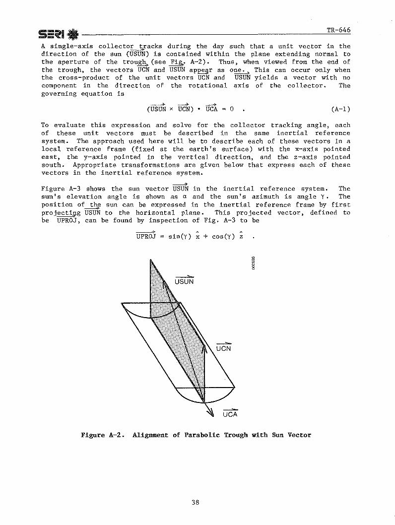
A single-axis collecto~racks during the day such that a unit vector in the direction of the sun (USUN) is contained within the plane extending normal to the aperture of the trough.r (see Fi~. A-2). Thus, when viewed from the end of the trough, the vectors UCN and USUN ap~r as one.~ This can occur only when the cross-product of the unit vectors UCN and USUN yields a vector with no component in the direction of the rotational axis of the collector. The governing equation is

--=r ~ ~

(USUN x UCN) • UCA o (A-I)

To evaluate this expression and solve for the collector tracking angle, each of these unit vectors must be described in the same inertial reference system. The approach used here will be to describe each of these vectors in a local reference frame (fixed at the earth's surface) with the x-axis pointed east, the y-axis pointed in the vertical direction, and the z-axis pointed south. Appropriate transformations are given below that express each of these vectors in the inertial reference system.

--=r Figure A-3 shows the sun vector USUN in the inertial reference system. The sun's elevation angle is shown as Ct and the sun's azimuth is angle y. The position of t~ sun can be expressed in the inertial reference frame by first projectipg USUN to the horizontal plane. This projected vector, defined to be UPROJ, can be found by inspection of Fig. A-3 to be

-----=r A

UPROJ = siney) x + cos(Y) z

<0 0>

§ ~

USUN

---.. UCA

Figure A-2. Alignment of Parabolic Trough with Sun Vector

38

S=~II*I _____________________ T_R_-6_46

y, vertical

X, east

--.:::.... USUN

UPROJ

.... $ 8 o

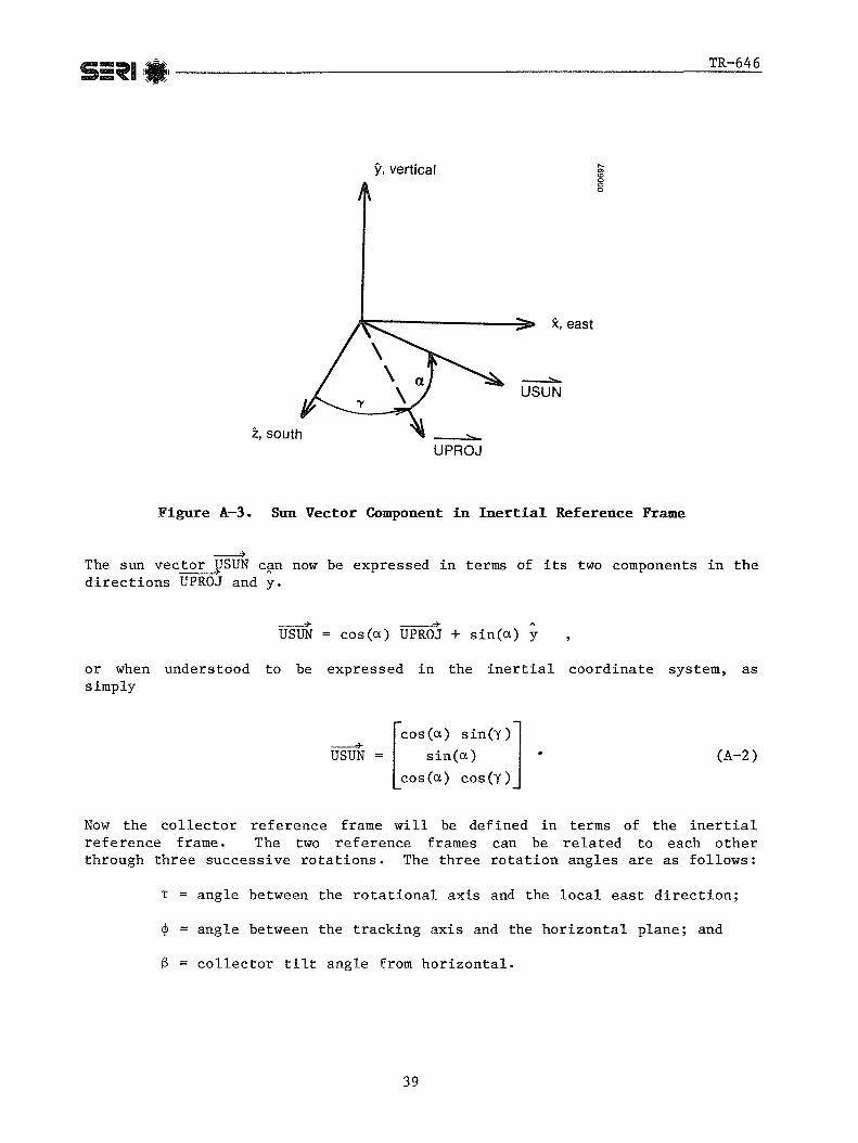
Figure A-3. Sun Vector Component in Inertial Reference Frame

__ or

The sun vector VSUN c~n now be expressed in terms of its two components in the directions UPROJ and y.

---=r ------.:r USUN = cos(a) UPROJ + sin(a) y

or when understood to be expressed in the inertial coordinate system, as simply

---=r USUN

[

COS (a) Sin(Y)J sin(a)

cos (a) cos (y )

(A-2)

Now the collector reference frame will be defined in terms of the inertial reference frame. The two reference frames can be related to each other through three successive rotations. The three rotation angles are as follows:

T angle between the rotational axis and the local east direction;

~ angle between the tracking axis and the horizontal plane; and

B collector tilt angle from horizontal.

39

55'1 1*1 ______________________ ...::.TR~-.....::6....:...:...46

The first reference frame transformation accounts for rotation of the trough axis horizontally away from east by the angle T. For an east-west rotational axis collector, T = O. For a north-south rotational axis, T = 900

• As illus­trated in Fig. A-4, the three orthogonal bases of the inertial reference frame are related to the orthogonal bases of the rotated reference frame as

where

A

z'

i, south

[

COS(T)

-S~n(T ) o I

o

y, vertical, y ,

(A-3)

X, east

Figure A-4. Rotation of Parabolic Trough Tracking Axis Away from Local East

40

S=~I TR-646

If the rotational axis of the collector is not horizontal, this can be accounted for with the next" coordinate transformation. Rotate up from the horizontal plane about the z I vector by the angle <p. This rotation (see Fig. A-5) is described by:

where

B

Z',2:"

["] ["] Xl I Xl

!" = B !I Z I I Zl

[

cos(<P)

-Sin(~)

y'

sin(<p)

cos(<P )

o

(A-4)

x"

x'

Figure A-S. Rotation of Parabolic Trough Tracking Axis ~ay from Horizontal

41

S=~II: ~ _______________________ T_R-_6_46

Finally. rotate about the x" vector by the angle S as shown in Fig. A-6. is the collector tilt angle rotation:

where

~

UCN,Y'"

[" J ["] x'" x"

r"' = C r" z'" z"

o cos(S)

-sin(S)

Si~(S)] . cos(S)

'I"

~

z '''. UCP

--=--UCA

x", x'"

8 § o

Figure A-6. Rotation of Parabolic Trough to Correct Tracking Angle

42

This

5 - 9 1 ' TR-646 =~ i, ~----------------------------------__ ~~~

The three orthogonal vectors ~"', Y"~+and ill' ar~~quivalent to the col­lector reference frame vectors DCA, DCN, and DCP, respectively (see Fig. A-I). Now, the collector reference frame can be related to the inertial reference frame by substituting Eqs. A-3 and A-4 into Eq. A-5:

[A] [A] x'" x

!'" = CBA ! z'" z

or

[

A ]

x" ,

( CBA) -1 ! ' " z" ,

(A-6)

-* -* We must define both DCN and DCA in terms of the inertial reference frame to solve Eq. A-I.

-* First, we define (DCN)i to be the vector normal to the collector expressed in the inertial reference system. We know that A in the collector coordinate system, the_~ollector normal vector has only a y'" component. Thus, we can solve for (DCN)i as

(DCN)i A-1B-1C-1 m [

-Sin(<j» cos (T) cos (S) - sin(T) Sin(s)] = cos(<j» cos(S) .

-sin(<j» sin(T) cos(S) + COS(T) sineS)

(A-7)

The trough rotational-axis vector can be similiarily defined in terms of the inertial reference system:

----* (DCAh

[

COS(<j» COS(T)] sin(<j» .

cos(<j» sin(T)

(A-8)

43

Si~I'*' ________________________ TR_--'..6_46

Now, substituting Eq. A-2, A-7, and A-8 into Eq. A-1:

[

cos(a) Sin(Y)j [-Sin(<l» COS(T) cosUs) -sin(a) x cos(<l» cos(S)

cos(<l» cos(y) -sin(<l» sin(T) cos(S) +

sin(T) sin(S )]

sin(S) COS(T)

[

COS(<l» COS(T)] • sin(<l» = 0

cos(<l» sin(T)

(A-9)

Multiplying through all the terms and solving for S (the collector tracking angle measured from horizontal) results in

= -1 ( COS(T) cos(y) cos(a) - sin(T) sin(<l» cos(a) ) Stan sin(a) cos(<l» - cos(a) sin(<l» [cos(<l» sin(T) + sin(<l» COS(T)] .

(A-10)

This equation reduces to a simpler form for east-west and north-south rota­tional-axis troughs mounted horizontally. For the horizontal east-west case) we have

t -l(COS(Y) cos(a)) an sin(a) .

For the horizontal north-south case, the expression is

t -l(-sin(y) cos(a)) an sin(a) .

Tracking Angle for Single-Axis Collector with Misaligned Sun Tracker

When a misaligned aperture-based sun tracker provides the tracking control of a single-axis collector, the collector will track the sun at slightly dif­ferent angles from those described in the preceding section. The angular mis­alignment that is of concern is denoted by the angle d in Fig. A-7. This mis­alignment means that the base of the shadow band of the sun tracker is not parallel with the rotational axis of the trough (as shown in Fig. A-2). The

44

TR-646

~ o g

--==-USB

---=-UCA

Figure A-7. Shadow-Band Misalignment Schematic

~

base of the shadow band is shown to define a unit~¥ctor USB which is slightly misaligned from the collector's rotational axis, UCA. The tracker head senses the position of the sun and provides an error signal of zero only when the sensors on each side of the shadow band are balanced. This "satisfied" position occurs when the tracking angle of the collector is such that the following equation is satisfied:

__ --=r --=r

(USUN x UCN) • USB = 0 (A-H)

This is identical to the governing equation (Eq. A-I) given earl!er for an aligned sun tracker, except that the shadow-band direction (USB) is used instead of the rotational axis of the collector.

Again, we must describe the three v~ctors~ Eq. A-II in terms of the inertial reference system. Th~_~ectors USUN and UCN are unchanged from the preceding section. The vector USB requires an additional rotation beyond those already given. This rotation of the shadow band by the angle 0 is illustrated in Fig. A-8. It is described mathematically as

where

D

[" 1 [A 1 x"" x'" ~"" = D ~'" , z"" z'"

[

cos(o)

-Si~(O ) 45

o I

o

Si~(O) 1 cos(o)

(A-12)

S=~II

Y III, y"l1

--"-UCN

---:.... UCA

-:....

USB, X ""

'" '" g o

TR-646

Figure A-S. Rotation of Parabolic Trough to Tracking Angle for Misaligned Shadow-Band Sensor

Now, the sun tracker reference frame can be described in terms of the inertial reference frame:

(USB)i is defined to be the shadow-band vector described in terms of the inertial reference system and is calculated as

(USB)i -1 -1 '-1 -1 [IJ ABC D 0 o

= [COS(T) cos(4))

cos(4)) sin(T)

COS(d) + sin(d) [sinO~) COS(T) sin(4)) - sin(T)

COS(d) sin(4)) - cos(4)) sin(l3) sin(d)

cos (d) + sin(d) [sin(4)) sin(T) sin(S) + cos(S)

Now, Eqs. A-2, A-7, and A-13 can be substituted into Eq. A-II:

cos(a) sin(Y)

sin(a) x

cos(a) cos(Y)

-sin(4)) COS(T) cos(S) - sin(T) sineS)

cos (4)) cos (S )

-sin(4)) sin(T) cos(S) + COS(T) sineS)

46

(A-13)

cos (S ) ]j. cos (T)]

5=~1'_' _____________________ .=TR:::.--~646

• [COS(T) cos(</»

cos (</» sin(T)

COS(d) + sin(d) [sin(f3) COS(T) sine</»~ - sin(T)

COS(d) sine</»~ - cos(</» sineS) sin(d)

COS(d) + sin(d) [sine</»~ sin(T) sineS) + cos(S)

cos (S ) J] = 0 .

cos (T) J

(A-14)

MUltiplying through all the terms and reducing the equation results in

COS(S)[COS(T) COS(d) cos(Y) cos(a) - sin(Y) cos(a) sin(T) COS(d)]

+ sin(S){ [COS(d) cos(a) sin(</»)(sin(T) cos(y) + sin(Y) cos(:r)J

- sin(a) cos(</» cos (d)}

- [sin(d) sin(T) cos(</» cos(Y) cos(a) + sin(a) sine</»~ sin(d)

+ cos (</» sin(Y) cos (a) sin (d) cos (T)] o (A-15)

This transcendental equation is solved by successively substituting for S. A good initial guess is defined by the no-misalignment solution for S given by Eq. A-10.

47

48

S=~II*I _______________________ T'-R'--6'--'-'46

APPENDIX B

SUN POSITION ALGORITHM

It is necessary to know the position of the sun, expressed in terms of azimuth and elevation, to calculate the correct tracking angle of a parabolic trough concentrating collector. The sun-position algorithm presented here has an accuracy of 0.01 degrees for the time period within five years of January 1980.

The azimuth of the sun measured from south, <p, and the elevation of the sun measured from horizontal, a, are calculated [7] from

and

where

sin(a) sin(L) sin(d) + cos(L) cos(d) cos(h)

cos(<P ) cos(d) sin(h)/cos(a)

L local latitude, d declination of the sun, h hour angle of the sun.

A formula for the sun's declination is given in Ref. 8 as

sin d = sin £ sin Ls

where the obliquity of the eliptic, £, is 23.442° for the years 1975 to 1983, and Ls is the longitude of the sun given (in degrees) by

where

Ls = Lo + 1.916 sin g - .020 sin 2g

L = .985647 T - 80.181° o

is the geometric mean longitude of the sun measured from the equinox, and

g = .9856 T - 2.777°

is the mean anomaly of the earth.

T is defined to be time, measured in days from midnight Greenwich Mean Time on 1 January 1980.

The hour angle of the sun, h, can be calculated (in degrees) as

h = (LST - 12) x 15° - local longitude + local meridian + bh

where LST is Local Standard Time, in hours, and bh is the equation of time.

49

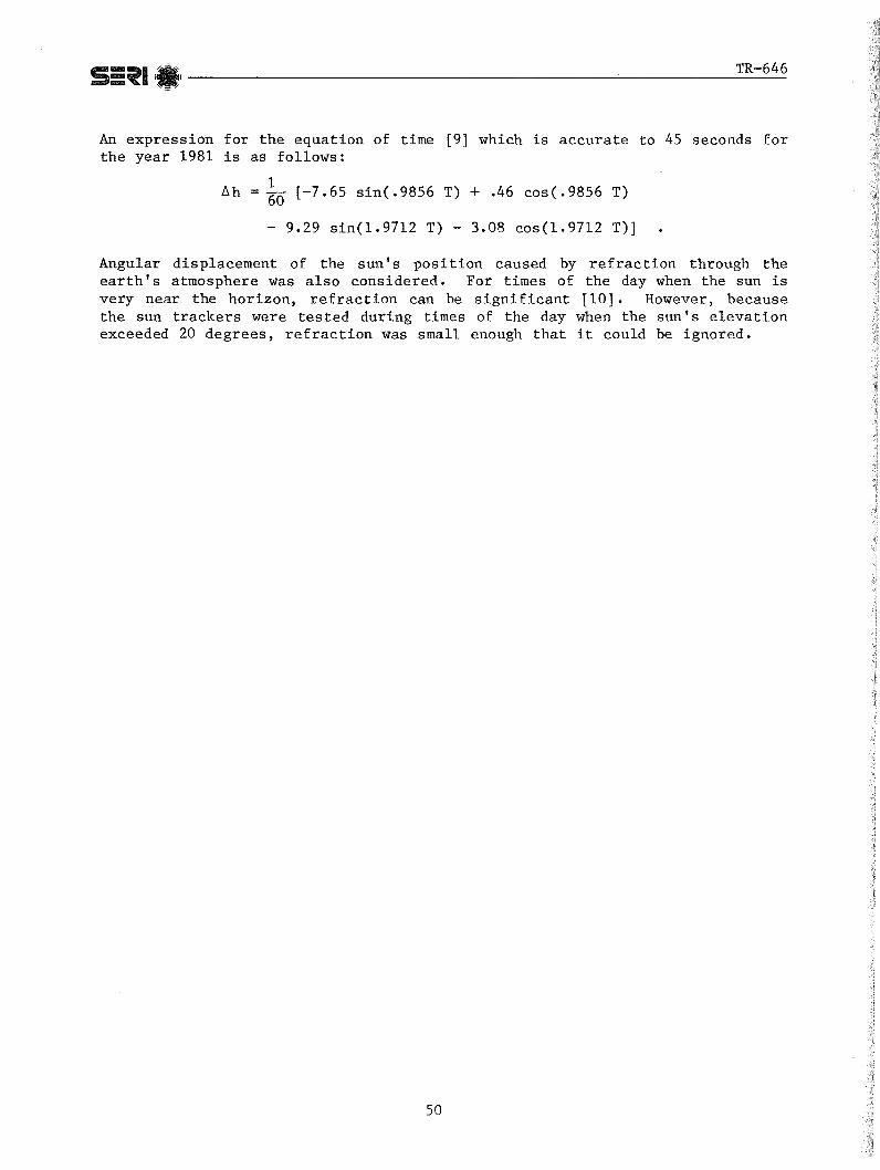
S=~II*J _________________ ---'---_____ T_R-_6_46

An expression for the equation of time [9] which is accurate to 45 seconds for the year 1981 is as follows:

~h = ~O [-7.65 sin(.9856 T) + .46 cos(.9856 T)

- 9.29 sin(1.97l2 T) - 3.08 cos(1.97l2 T)]

Angular displacement of the sun's position caused by refraction through the earth's atmosphere was also considered. For times of the day when the sun is very near the horizon, refraction can be significant [10]. However, because the sun trackers were tested during times of the day when the sun's elevation exceeded 20 degrees, refraction was small enough that it could be ignored.

50

S=~II_I ______________________ -=T=R=---6::.....:..,:46

APPENDIX C

PARABOLIC TROUGH ANNUAL PERFORMANCE MODEL

A long-term average uti lizability method [11] was used to compute the impact of tracking error on the annual performance of a parabolic trough concen­trating collector. Basically, the utilizability method involves computation of the long-term average energy delivery of a parabolic trough for the central day of each month of the year; these monthly values are then summed to an annual total. The procedure was modified significantly to account spe­cifically for the optical characteristics of parabolic troughs.

The average monthly energy collection ECQII m the day-long average optical efficiency <.no~' insolation Rcoll .

is computed as the product of utilizability ~, and available

where N = number of days in the month.

The all-day available insolation Rcoll is calculated by integrating the pro­duct of the beam insolation and the cosine of the incidence angle on the col­lector in the following way:

The calculation of <no> requires efficiency at 00 incidence, no' and available beam insolation Ibcos8i in

w

Ib cos8 i dw (C-I)

weighting the product of the optical the incidence angle modifier K(8) to the the following fashion:

<n > o

J c

O [IbcOS 8.] n K(8) dw

~ 0 (C-2) w

J c Ib cos 8. dw o 1

The incidence angle modifier K(8) defines how the optical efficiency decreases with incidence angle relative to the trough's normal incidence optical effi­ciency. Several factors contribute to the decrease of optical efficiency with increasing incidence angle. These factors include, in part, the angular dependence of glass annulus transmittance and receiver absorptance. Also, the intercept factor (defined as that fraction of rays incident upon the aperture that reaches the receiver) decreases with incidence angle. This decrease in optical efficiency due to a reduction in intercept factor is brought about in two ways. First, beam spreading occurs because of longitudinal contour and nonspecularity errors. Second, the apparent sun image becomes wider because of the longer reflected path length.

51

S=~II*I _____________________ -=-TR:.::....-~646.

Calculation of the intercept factor Y involves the convolution of the geo­metric angular acceptance function for a parabolic trough with a Gaussian dis­tribution that accounts for total beam spreading (i.e., both optics and sun size). As shown by Rabl et al. [5], the intercept factor Y can then be expressed as a function of the product of ° total and C. C is the geometric concentration ratio of the trough, defined as:

w C ----

1f Dabs

° total is the total rms angular beam spread of the reflected beam from the concentrator to the receiver. It is calculated as

( 2 2 )1/2 °total = °optical + °sun

where

°optical 2 2 ( 2 2 )

4ocontour + 0.215 tan 6 i 4ocontour + 0specular

2 2 + ° track + ° specular

2 + ° disp

°sun = 2

0sun noon/cos (8 i ) ,

The sun's rms angular width typically is taken as 2.8 mrad.

After both C and ° total are defined, the intercept factor can be calculated for a 90° rim angle trough with the following equation (curve-fit to Fig. 4-3):

1 for ° total C " 0.134

Y [oC]= [0.932 + 1.27 ° totalC - 6.54(ototalC) 2

+ 3 5.91(ototalC) ]

for 0.1314 < °totalC " 0.45

[1. 38 - 2.01 °totalC + 1. 35 (0 total C) 2 3

- 0.348(ototalC) ]

for 0totalC > 0.45

The angular dependence of transmittance and absorptance are extracted from data contained in the appendix to Ref. 12. The effect on absorptance from the distribution of incidence angles circumferentially on the receiver tube is included as well.

A utilizability function ~ is defined and the variability of the weather. centrating collector is a function intensity ratio X:

to account for both the daily heat loss This uti lizabi lity function for a con­of clearness index Kh and critical

The clearness index Kh is a site-specific parameter. Monthly values for Kh are listed in Ref. 13 for a large number of locations. For the results shown in Fig. 4-2, Kh values for Denver, Colorado, were assumed. However, other

52

TR-646

cities' corresponding Kh values will perturb the sensitivity of trough annual performance to tracking error only slightly.

The critical intensity ratio X is the ratio of the daily loss to that fraction of the incident solar energy received by the absorber. This ratio is given as

X UL (Tavg - Tamb) 2 tc

<no>C Hcoll

The heat-loss coefficient UL is a function only of the receiver charac­teris tics. Note that it is defined in terms of absorber tube surface areaZ For the results shown in Fig. 4-2, a UL(Tav - Tamb ) product of 1500 W/m absorber was assumed. This value is typic3t of the heat-loss rate from parabolic trough receivers operating at about 200°C [14]. Again, other choices for receiver heat-loss rate alter the tracking error results of Fig. 4-2 only slightly.

Equations C-l and C-2 are integrated numerically. cutoff hour angle w c is not known and is found maximize the monthly collector energy output.

53

However, the value of the by iteration in order to

54

S=~I

c

Ecoll

E coll,m

w

x

y

e bias

e calculated

(3 track error

e. 1

NOMENCLATURE

geometric concentration ratio (= W/~ Dabs)

absorber tube outside diameter

TR-646

average annual energy collection (per unit of collector area) of an unshaded collector

average monthly energy collection (per unit of collector area) of an unshaded collector

irradiation incident on collector aperture area on a daily basis

beam irradiance

clearness index

incidence angle modifier

cutoff time measured as hours from solar noon

ambient temperature

absorber tube surface temperature

heat-loss coefficient, based on absorber tube surface area (li/m2 °C)

concentrator aperture width

critical intensity ratio for utilizability method

intercept factor

optical efficiency at normal incidence

average optical efficiency on a daily basis

experimentally measured collector tracking angle

angular bias between actual and calculated tilt angles over test period due to incremental encoder position

calculated tracking angle of collector

instantaneous tracking error of a given data point

rms angular spread due to tracking error expected for a given instantaneous direct normal irradiance

incidence angle of beam irradiance on collector

55

!i::~1 'JI' __________________________________________________________ ~T~R_-~6~4~6

o contour

o disp

o . 1 optlca

o specular

°sun

o sun,e i=O

o track

w

a

T

a

rms angular devLiition of coneelltrator from perfect parabo1.a (slope error)

equivalent rms angular spread, which accounts for imperfect placement of receiver

rms angular spread due to all optical errors (at normal incidence)

rms angular spread of reflected beam due to imperfect specularity of reflector material

rms angular width of sun (as viewed by receiver)

rms sun shape at incidence angle of zero (2.8 mrad)

total rms beam spread

rms angular spread due to tracking error (effective annual value)

uti lizabi lity

hour angle

cut-off hour angle

elevation angle of sun

angle between the rotational axis of a trough and the local east direction

collector tilt angle measured from the horizontal plane

horizontal offset of trough measured from the rotational axis of the trough to the horizontal plane

angular misalignment of a shadow-band sun tracker

56

5=~1'_' _________ -'--____________ -=T=R~-6~46

Vectors in Appendix A

~

UCA

~

UCP

--UPROJ

~

USB

-USUN

unit vector that defines the direction of the rotational axis of the collector

unit vector that defines the direction normal to the aperture of the collector

unit vector that defines the direction of the aperture of the collector

projection of the sun vector onto a horizontal plane

unit vector that defines the direction of the shadowing plate for a shadow-band sun tracker

unit vector that defines the direction of the sun

57

Document Control j ~ SERI Report No. 12. NTIS Accession No.

Page SERI/TR-632-646 4. Title and Suotltle

An Experimental Performance Evaluation of Line­Focus Sun Trackers

7. Autnor( s)

Randv C. Gee 9. Performing Organization Name and Aacress

Solar Energy Research Institute 1617 Cole Boulevard Golden, Colorado 80401

12. Sponsonng Organization Name and Address

15. Supplementary Notes

3. RecIpient's Accession No.

5. Publication Date

fvlay 1982 6.

8. Performing Organization RepL No.

10. ProjectlJ'ask/Work Unit No.

1007.99 11. Contract (C) or Grant (G) No.

(C)

(G)

13. Type of Report &. Period Coveree

TechniCrt1 Report 14.

16. Abstract (Lim!!: 200 wores) Two sun trackers have been tested for tracki ng accuracy on an outdoor test stand. One was a shadowband sun tracker and the other was a flux-linE sun tracker. Both performed well during the entire test period. Their tracking performance as a function of insolation level was established, and their overall tracking accuracy (rms tracking error) was calculated. Both the flux-line and the shadowband tracker were found to have an effective rms error of about 1 milliradiar This information was used to determine the impact that the two trackers have on the annual energy performance of typical parabolic trough concentrating collectors. One milliradian rms tracking errors were found to result in negligibly small annual performance losses.

17. Document Analysis

a. DeSCriptors Paral:olic trough collectors ; Solar tracking ; Perfonnance testing

b. Identifiers/Open-Ended Terms Shadow-band sun trackers ; Plux-line sun trackers ; tracking error

c. UC Categories

59, 62

,9. No. of Pages 18. Avallaoiiity Statement National Technical Information Service 67 U.S. Department of Commerce 5285 Port Royal Road <;nrinnfil"lrl \f;rniniri 2:;>161

20. Price

$5.25 Form No. a200-~3 :6-i9\

'A-t,!.s. GOVERNMENT PRINTING OFFICE: 1982-0-576-083/107

DATE DUE

r::i:"D-:i-: _~q;'r:t -

DEMeo 38-297

i

1 1 !

SERI/TR-632-646 C.3 GEE} R.C.

AN EXPERIMENTAL PERFOR­MPd'J.CE EVP,LUATHJN OF I INF,·, FOCUS SUN TRACKERS. _. -

SOLAR ENERGY RESEARCH INSTITUTE

SOLAR ENERGY INFORMATION

CENTER

GOLDEN, COLORADO 80401