ORIGINAL ARTICLE

An experimental characterization of reservoir computingin ambient assisted living applications

Davide Bacciu • Paolo Barsocchi • Stefano Chessa •

Claudio Gallicchio • Alessio Micheli

Received: 10 July 2012 / Accepted: 21 February 2013

� Springer-Verlag London 2013

Abstract In this paper, we present an introduction and

critical experimental evaluation of a reservoir computing

(RC) approach for ambient assisted living (AAL) applica-

tions. Such an empirical analysis jointly addresses the

issues of efficiency, by analyzing different system config-

urations toward the embedding into computationally con-

strained wireless sensor devices, and of efficacy, by

analyzing the predictive performance on real-world appli-

cations. First, the approach is assessed on a validation

scheme where training, validation and test data are sampled

in homogeneous ambient conditions, i.e., from the same set

of rooms. Then, it is introduced an external test set

involving a new setting, i.e., a novel ambient, which was

not available in the first phase of model training and vali-

dation. The specific test-bed considered in the paper allows

us to investigate the capability of the RC approach to

discriminate among user movement trajectories from

received signal strength indicator sensor signals. This

capability can be exploited in various AAL applications

targeted at learning user indoor habits, such as in the

proposed indoor movement forecasting task. Such a joint

analysis of the efficiency/efficacy trade-off provides novel

insight in the concrete successful exploitation of RC for

AAL tasks and for their distributed implementation into

wireless sensor networks.

Keywords Ambient assisted living � Reservoir

computing � Wireless sensor networks � Indoor user

movement forecasting

1 Introduction

Ambient assisted living (AAL) [1] is a recent research

program issued by the European Community. It addresses

those technologies that can be used to improve the quality

of life of elders or disabled by assisting them and making

them feel secure and protected in the places where they live

or work. The AAL effort is strongly motivated by the fact

that the number of elders in the European Community is

constantly increasing, and a large demand of AAL-related

technologies is expected in the near future. AAL applica-

tions typically rely on a number of devices, equipped with

sensing capabilities that provide data which serve to detect

events occurring around or to the user. In order to facilitate

the user acceptance of AAL technologies, these devices,

typically referred to as sensors, should be of reduced size

(especially those deployed on the user itself) and make

large use of wireless communication technologies. A

wireless sensor network (WSN) for AAL comprises a

variable number of tiny sensors, each of which is a micro

system embedding a processor/memory subsystem, a set of

transducers, a radio subsystem and a battery. Sensors can

self-organize in order to build and maintain a wireless

network for their communications.

D. Bacciu � S. Chessa � C. Gallicchio (&) � A. Micheli

Dipartimento di Informatica, Universita di Pisa, Pisa, Italy

e-mail: gallicch@di.unipi.it

D. Bacciu

e-mail: bacciu@di.unipi.it

S. Chessa

e-mail: ste@di.unipi.it

A. Micheli

e-mail: micheli@di.unipi.it

P. Barsocchi

Istituto di Scienze e Tecnologie dell’Informazione,

Consiglio Nazionale delle Ricerche, Pisa, Italy

e-mail: paolo.barsocchi@isti.cnr.it

123

Neural Comput & Applic

DOI 10.1007/s00521-013-1364-4

A WSN can deliver consistent amounts of data to an

AAL system, providing a very crude picture of the envi-

ronment/user being monitored. As such, consistent refine-

ment of the sensed data is needed in order to extract the

high-level information, e.g., user activities or events, that is

best suited to processing within an AAL system. Given the

peculiarities of the information involved, this process

requires an approach characterized by adaptivity and

robustness to input noise. Within this scenario, Machine

Learning models, in general, and Neural Networks, in

particular, provide feasible data-driven solutions. We focus

on recurrent neural networks (RNNs) [25], representing

dynamical neural network models capable of directly pro-

cessing the temporal streams of sensed data produced by

the nodes of the WSN. Within such RNN class, we con-

sider the Reservoir Computing (RC) paradigm [30, 41] and,

more specifically, the echo state network (ESN) model

[22, 23]. ESN feature an interesting trade-off between

extreme computational efficiency and the ability to learn in

temporal sequence domains.

In view of a complete integration between the devices of

a WSN and the learning capabilities offered by the RC

networks, we envisage a system in which the learning

models are embedded directly on-board the nodes of the

WSN. However, learning in distributed WSN systems for

AAL tasks raises novel challenges related to the effec-

tiveness and efficiency in treating the sensed (temporal)

data. RC has the potential for providing learning solutions

that are effective in terms of time series prediction accu-

racy, given the RC ability of capturing complex time-

dependent behaviors in its reservoir state, yet efficient from

the point of view of computational and memory require-

ments. As such, they are good candidates for the devel-

opment of computational learning models that can be

embedded on the WSN devices. Such devices have limited

computational capabilities, but provide direct access to

sensor data, either acquired by the on-board transducers or

received from neighboring sensors through the wireless

radio. An embedded RC model can thus be trained to

provide an on-board preprocessing of the sensorial infor-

mation to predict refined information concerning the

environment/user state. This, on the one hand, reduces the

communication burden, since only high-level predictions

are transferred to the (typically centralized) AAL system

through the wireless communication media. On the other

hand, it allows to distribute the computational burden,

relieving the central AAL system from the processing of

the low-level sensor information.

The deployment of such an innovative distributed

embedded learning system needs to be anticipated by an

empirical assessment of the RC neural models, to deter-

mine their suitability in addressing AAL-related tasks.

Current works in literature propose experimental analyses

that are fairly limited in scope and, basically, found on the

sole use of artificial data. In this concern, a benchmarking

of the RC approach is still needed, with particular regard to

the assessment of the effectiveness on real-world data and

the evaluation of the efficiency of the learning models. To

this aim, we consider a computational learning task that

follows from a representative AAL problem, i.e., the pre-

diction of the indoor user spatial context in the monitored

environment. This is one of the most critical information

required by an AAL system, which is essential to deliver

the services to the user in the appropriate place and at the

right time. The user trajectory information can be easily

collected, in the form of time series, by measuring the radio

signal strength (RSS) among a few wireless devices

deployed in the environment and a user wearable sensor.

As it will be discussed in Sect. 2, such real-world

task involves streams of noisy input data and requires the

ability to appropriately adapt to specific user/environment

conditions.

Motivated by the above-mentioned RSS-localization

challenges and, more in general, by the study of the design

of WSN-embedded learning systems for AAL tasks, we

propose a novel RC approach to indoor movement fore-

casting that aims at predicting the future user context based

on real-world noisy RSS input data. This work presents a

systematic experimental investigation of the RC approach

that jointly considers both the efficiency and the efficacy of

proposed solution in a real-life AAL application. A sys-

tematic assessment of the RC approach requires solid data,

gathered on a realistic scenario that is consistent with the

task to be addressed. To this end, we have devised a real-

life localization benchmark, comprising a small WSN

network capturing localization information in different

experimental premises and whose details are given in Sect.

4.1. The proposed benchmark focuses on learning to dis-

criminate among different types of user trajectories based

on RSS measurements across time. Such task is associated

to a specific semantics in AAL applications, related to the

forecasting of the user spatial context, i.e., room change vs.

room preservation. This is intended to be a concrete use

case for an RC approach capable of addressing diverse

AAL tasks associated to learning user indoor activity

habits. A through evaluation cannot abstract from an

appropriate validation scheme, tailored to the identification

of the major properties of the learning model with respect

to the application at hand. In this sense, it is worth to

evaluate the ability of the RC approach in generalizing its

prediction performance to novel, unknown, environments.

Such property is needed to show that, while the proposed

solution can increase the level of service personalization

(i.e., by making accurate prediction of the user spatial

context), it can, at the same time, yield to a reduction of the

setup and installation costs by means of adequate

Neural Comput & Applic

123

generalization capabilities. In view of a distributed

embedded realization of the neural system, efficiency is a

relevant desirable property that should be considered and

assessed. Hence, in this paper, we specifically evaluate the

trade-off between predictive accuracy and memory occu-

pation cost, which is central to embed learning modules on

low-power WSN devices. In this sense, the RC paradigm

offers an interesting ground due to its intrinsic character-

istic of efficiency: in this paper, we discuss an empirical

assessment of the relation between the performance and the

implementation cost of constrained RC networks. In par-

ticular, using a lightweight scheme for storing the untrained

reservoir weights, we consider the effect of reservoir

dimensionality, which has a direct impact on both predic-

tive accuracy and memory occupation cost. Additionally,

we explore the performance of modular neural architec-

tures, coherent with the WSN-distributed structure, com-

prising independent learning modules that can share

information through the WSN communication media.

Various degrees of learning interactions are discussed and

experimentally assessed, including cases of full and partial

connectivity, as well as committee architectures.1

The remainder of the paper is articulated as follows:

Sect. 2 discusses the background on RSS-based localiza-

tion and available learning-based solutions; Sect. 3

describes the detail of the RC model, while Sect. 4 dis-

cusses the localization benchmark and the results of the

experimental assessment; Sect. 5 concludes the paper.

2 Background

AAL applications normally operate in indoor environments

and require localization services. However, these services

can hardly be supported by established global positioning

systems (such as GPS or Galileo) that do not provide the

appropriate accuracy in indoor environments. For this

reason, localization information is generally obtained by

means of other technologies, based on sensors or cameras

deployed in the user environment. In the attempt to deliver

cost-effective localization services, researchers tend to

privilege the use of widely available technical solutions

exploiting off-the-shelves components, and generally avoid

the use of cameras, that may present user acceptance issues

[14], as they are more invasive on the user life.

A practical solution for indoor user localization consists

in using a number of fixed, environmental sensors whose

position is known (these sensors are called anchors) and a

wearable sensor (also called mobile sensor) that is con-

stantly carried by the user. The anchors and the mobile

frequently exchange radio packets (called beacons) and, for

each beacon, they measure the corresponding strength of

the radio signal (called RSS). Since the strength of the

signal decays with the distance between the source and the

receiver, it is possible to relate a RSS associated to a

beacon, with the distance between the anchor and the

mobile that exchanged that beacon. Hence, a localization

system can, in principle, exploit the RSS information col-

lected over a period of time, to predict an approximated

user position. Unfortunately, the propagation of the radio

signals in indoor environments is subjected to phenomena

that may alter significantly the RSS measure depending on

the specific setting of each room. Additionally, the RSS

measurements are greatly affected by the relative position

of the user with respect to the line of sight between the

anchor and the mobile. Nevertheless, RSS-based localiza-

tion is a cost-effective solution for localization of users in

indoor AAL applications, due to the widespread deploy-

ment of wireless networks and WSN infrastructures that

make available RSS measurements. Mainly, we distinguish

between two alternative computational approaches to

localize users leveraging the RSS measurements, i.e.,

model-based and fingerprinting positioning.

Model-based positioning is popular approach in literature

that founds on expressing radio frequency signal attenuation

using specific path loss models [7, 8]. Given an observed RSS

measurement, these methods triangulate the person based on

distance calculations from multiple anchors. However, the

relationship between the user position and the RSS informa-

tion is highly complex and can hardly be modeled due to

multipath, metal reflection and interference noise. Thus, RSS

propagation may not be adequately captured by a fixed

invariant model. In these conditions, it is not surprising that

such analytical models fail to reach acceptable accuracy

levels, with typical localization errors ranging between 2 and

4 m (depending on the setting) [14].

Differently from model-based approaches, fingerprint-

ing techniques, such as [6, 27, 35, 44], create a radio map

of the environment based on RSS measurements at known

positions by means of an offline map-generation phase.

Clearly, the localization performance of fingerprinting-

based model relies heavily on the choice of the distance

function that is used to compute the similarity between the

RSS measured in the online phase, with the known RSS

fingerprints. Further, the offline-generated ground truth

might need to be revised in case of changes to the room/

environment configuration, which might result in relevant

discrepancies in the known fingerprints.

1 This paper, based on ex-novo conducted experiments, extends the

preliminary investigations presented in the conference papers [18],

proposing a comprehensive vision of the costs that can practically

occur for real deployment of the RC models into mote devices. In

particular, previous works did not include an exhaustive comparative

analysis of different network sizes and configurations [4, 18], or the

adoption of a reduced reservoir weight-encoding scheme [4, 18] or the

external performance evaluation [18].

Neural Comput & Applic

123

Adaptivity and flexibility with respect to minor envi-

ronmental changes can be introduced in the fingerprinting

approach, by exploiting computational learning models to

infer the relationship between the RSS samples and the

subject location. The majority of the approaches in litera-

ture exploit probabilistic learning techniques to learn a

posterior estimate of user location given RSS measure-

ments at known location, e.g., [29, 45]. However, proba-

bilistic models have consistent computational costs

connected both with the learning and the inference phase,

which might grow exponentially with the number of sen-

sors in the area. k-nearest neighbor (kNN) algorithms often

show good accuracy which, however, tends to be particu-

larly sensitive to beacon positioning [31]. Nevertheless,

kNN is characterized by well-known expensive memory

and computational requirements which make it less suit-

able for embedding in WSN nodes. Similar complexity

considerations apply to the use of Multi Layer Perceptrons

[9] and Support Vector Machines [11, 43] in location fin-

gerprinting, that is mainly limited to wireless local area

networks of powerful access points and palmtop devices.

The measurement of RSS values over time provides

information on the subject trajectory under the form of a

time series of sampled signal strength, which allows for

subject tracking rather than simple localization. However,

neither the static RSS-map of the fingerprinting approaches

discussed so far nor the predefined propagation model of

model-based solutions is appropriate to capture such

dynamic knowledge. The adaptive fingerprinting approa-

ches discussed above, for instance, do little to exploit the

sequential nature of the RSS streams, whereas they provide

static pictures of the actual state of the environment. More

importantly, these localization approaches can only provide

the estimate of the current user position, but lack the ability

of forecasting his/her future location. Being capable of

predicting the future user context is of a great added value

in AAL applications, since it enhances service reactivity

and personalization. In this respect, there exist several

machine learning models capable of explicitly dealing with

signals characterized by such time-dependent dynamics

including, for instance, probabilistic Hidden Markov

Models (HMM), RNN [25] and kernel methods for

sequences [19]. Kontkanen et al. [26], for instance, discuss

the application of HMMs to tracking using RSS informa-

tion: their use in computationally constrained devices is,

however, limited by the complexity of the inference pro-

cess needed at test time. Similar problems occur in Kernel

Methods for sequences, whose cost scales at least qua-

dratically with the input length, e.g., Gartner [19].

ESNs [22, 23] are an RC model well suited for sequence

processing. Their most striking feature is efficiency:

training is limited to the linear outputs whereas the

dynamic part of the network is fixed. Additionally, the cost

of input encoding scales linearly with the length of the

sequence for both training and test (assuming a fixed

number of incoming recurrent connections for each reser-

voir unit, see Sect. 3), comparing favorably with compet-

itive state-of-the-art learning models for sequence domains.

For example, in Obst [33], it is proposed a research line in

which ESNs are used to detect misbehavior of the sensors

in a WSN. More in general, recently, ESNs have shown

good potential in a range of tasks related to autonomous

systems modeling, also by virtue of their marked effi-

ciency. Examples include event detection and localization

in autonomous robot navigation [2, 3], multiple robot

behavior modeling and switching [42], robot behavior

acquisition [21] and robot control [34]. However, such

applications are mostly focused on modeling robot

behaviors and often use artificial data obtained by simu-

lators [2, 3, 42]. More recently, Gallicchio et al. [18] have

proposed an ESN application to user’s indoor movements

forecasting using real-world data, followed by a pre-

liminary investigation of its generalization ability to unseen

ambient configurations by Bacciu et al. [4], where, how-

ever, efficiency issues are not taken into consideration.

Further differences with respect to these previous

approaches are summarized in Sect. 1 (see in particular

footnote 1).

The latter works demonstrates the potential of the ESN

approach for RSS-based tracking, but miss a systematic

performance evaluation, especially with regard to the

constraints and possible configurations imposed by a dis-

tributed low-power environment such as WSN. In the fol-

lowing, we provide a thorough empirical assessment of

several distributed ESN configurations, based on realistic

WSN-induced layouts, with application to user movement

forecasting using real-world RSS data, in both homoge-

neous and heterogeneous validation settings (see Sect. 4)

3 Reservoir computing and echo state networks

RC [30, 41] represents an increasingly popular paradigm

for efficiently modeling RNNs. RC networks implement

dynamical systems and are essentially based on the sepa-

ration between a recurrent dynamical reservoir and a non-

recurrent readout. The role of the reservoir is to encode the

history of the input signals which drive the system. At each

time of computation, such network state provides the

readout with a rich set of ‘‘reservoir’’ dynamics, from

which to linearly combine in order to compute the output.

The outstanding feature of RC is the extreme efficiency of

training. Indeed, the simple readout component is the only

trained part of the network, while the reservoir is left

untrained after contractive initialization. RC comprises

several approaches, including the popular ESNs [22, 23],

Neural Comput & Applic

123

Liquid State Machines [32] and BackPropagation Decor-

relation [37, 38], among the others. In particular, in this

paper, we focus on the ESN model.

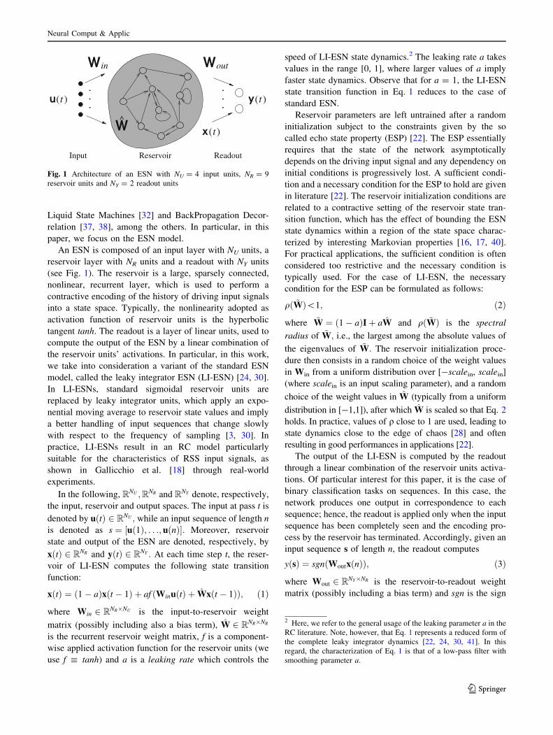
An ESN is composed of an input layer with NU units, a

reservoir layer with NR units and a readout with NY units

(see Fig. 1). The reservoir is a large, sparsely connected,

nonlinear, recurrent layer, which is used to perform a

contractive encoding of the history of driving input signals

into a state space. Typically, the nonlinearity adopted as

activation function of reservoir units is the hyperbolic

tangent tanh. The readout is a layer of linear units, used to

compute the output of the ESN by a linear combination of

the reservoir units’ activations. In particular, in this work,

we take into consideration a variant of the standard ESN

model, called the leaky integrator ESN (LI-ESN) [24, 30].

In LI-ESNs, standard sigmoidal reservoir units are

replaced by leaky integrator units, which apply an expo-

nential moving average to reservoir state values and imply

a better handling of input sequences that change slowly

with respect to the frequency of sampling [3, 30]. In

practice, LI-ESNs result in an RC model particularly

suitable for the characteristics of RSS input signals, as

shown in Gallicchio et al. [18] through real-world

experiments.

In the following, RNU ;RNR and RNY denote, respectively,

the input, reservoir and output spaces. The input at pass t is

denoted by uðtÞ 2 RNU ; while an input sequence of length n

is denoted as s ¼ ½uð1Þ; . . .; uðnÞ�: Moreover, reservoir

state and output of the ESN are denoted, respectively, by

xðtÞ 2 RNR and yðtÞ 2 R

NY : At each time step t, the reser-

voir of LI-ESN computes the following state transition

function:

xðtÞ ¼ ð1� aÞxðt � 1Þ þ af ðWinuðtÞ þ Wxðt � 1ÞÞ; ð1Þ

where Win 2 RNR�NU is the input-to-reservoir weight

matrix (possibly including also a bias term), W 2 RNR�NR

is the recurrent reservoir weight matrix, f is a component-

wise applied activation function for the reservoir units (we

use f : tanh) and a is a leaking rate which controls the

speed of LI-ESN state dynamics.2 The leaking rate a takes

values in the range [0, 1], where larger values of a imply

faster state dynamics. Observe that for a = 1, the LI-ESN

state transition function in Eq. 1 reduces to the case of

standard ESN.

Reservoir parameters are left untrained after a random

initialization subject to the constraints given by the so

called echo state property (ESP) [22]. The ESP essentially

requires that the state of the network asymptotically

depends on the driving input signal and any dependency on

initial conditions is progressively lost. A sufficient condi-

tion and a necessary condition for the ESP to hold are given

in literature [22]. The reservoir initialization conditions are

related to a contractive setting of the reservoir state tran-

sition function, which has the effect of bounding the ESN

state dynamics within a region of the state space charac-

terized by interesting Markovian properties [16, 17, 40].

For practical applications, the sufficient condition is often

considered too restrictive and the necessary condition is

typically used. For the case of LI-ESN, the necessary

condition for the ESP can be formulated as follows:

qð ~WÞ\1; ð2Þ

where ~W ¼ ð1� aÞIþ aW and qð ~WÞ is the spectral

radius of ~W; i.e., the largest among the absolute values of

the eigenvalues of ~W: The reservoir initialization proce-

dure then consists in a random choice of the weight values

in Win from a uniform distribution over [-scalein, scalein]

(where scalein is an input scaling parameter), and a random

choice of the weight values in W (typically from a uniform

distribution in [-1,1]), after which W is scaled so that Eq. 2

holds. In practice, values of q close to 1 are used, leading to

state dynamics close to the edge of chaos [28] and often

resulting in good performances in applications [22].

The output of the LI-ESN is computed by the readout

through a linear combination of the reservoir units activa-

tions. Of particular interest for this paper, it is the case of

binary classification tasks on sequences. In this case, the

network produces one output in correspondence to each

sequence; hence, the readout is applied only when the input

sequence has been completely seen and the encoding pro-

cess by the reservoir has terminated. Accordingly, given an

input sequence s of length n, the readout computes

yðsÞ ¼ sgnðWoutxðnÞÞ; ð3Þ

where Wout 2 RNY�NR is the reservoir-to-readout weight

matrix (possibly including a bias term) and sgn is the sign

.

.

.

.

.

.

ReadoutInput Reservoir

tuoni

(t )

(t ) (t )

Fig. 1 Architecture of an ESN with NU = 4 input units, NR = 9

reservoir units and NY = 2 readout units

2 Here, we refer to the general usage of the leaking parameter a in the

RC literature. Note, however, that Eq. 1 represents a reduced form of

the complete leaky integrator dynamics [22, 24, 30, 41]. In this

regard, the characterization of Eq. 1 is that of a low-pass filter with

smoothing parameter a.

Neural Comput & Applic

123

threshold function, such that yðsÞ 2 f�1;þ1g: The weight

values in Wout are typically trained using efficient linear

methods such as Moore–Penrose pseudo-inversion and

ridge regression [30, 41].

The reservoir dimensionality is an RC hyper-parameter

with a strong influence on both the network performance

and the computational cost. While larger reservoirs often

lead to better predictive performances in applications [17,

41], the cost of the ESN implementation grows with the

reservoir dimension both in time and in memory. In par-

ticular, due to the sparsity of reservoir units connectivity,

the cost can be linear assuming a fixed maximum number

of connections for each reservoir unit, or it is quadratically

bounded more in general. This point assumes an even

greater relevance in sight of the embedding of the RC

networks directly on-board the devices of a WSN. Such a

lightweight implementation of the reservoir network

modules on the sensors represents a challenging design

target [13], due to the severe computational constraints

involved (WSN sensors are equipped with a very small

amount of total RAM memory, typically in the range of

8–10 kbytes) and requires a careful assessment of the

trade-off between the implementation cost and the pre-

dictive performance of the RC networks in real-world

scenarios. The relation between the effectiveness and the

memory occupation cost of RC networks for AAL tasks is

investigated in this paper by experimentally evaluating

the effect of reservoir dimensionality on the accuracy

achieved by the LI-ESN model on a real-world task

described in Sect. 4. Moreover, we adopt an efficient

strategy for the memorization of the weight values in

matrices Win and W; using a small finite weight alphabet

for the nonzero weight values, which can thereby be

encoded using only a few bits. For instance, only 3 bits

per weight are required if we consider a weight alphabet

with 8 possible values.

Note that the use of a small finite alphabet of weight

values for the connections pointing to the reservoir can be

traced back to the early works in RC literature [22]. In this

paper, this reservoir initialization procedure is exploited

with the challenging objective of an extremely efficient

implementation of the RC modules directly on-board the

sensors of a WSN. Although a study of the architectural

pattern of connectivity among the reservoir units is out of

the scope of our paper, the proposed efficient weight-

encoding scheme can be related and applied also to

architectural variants of the standard ESN model, such as

reservoir architectures based on permutation matrices

[10, 20], self-recurrent connections only [15, 17] or cyclic

patterns of connectivity [36]. Finally, it is interesting to

observe that the proposed light-weighted encoding scheme

for the reservoir weight connections in a sense results in a

quantization of the space of weight values for the reservoir

part of the RC model. Although not directly connected to

this aspect, related literature approaches also consider the

quantization of reservoir state spaces [12, 39].

4 Benchmarking RC in indoor user movement

prediction

In the following, we describe a benchmark for adaptive

user movement prediction using RSS traces in a real-life

office scenario. First, in Sect. 4.1, it is provided a brief

discussion of the wireless technology involved, together

with a detailed description of the experimental indoor

environment. In Sect. 4.2, the RC approach described in

Sect. 3 is empirically assessed on the proposed forecasting

benchmark, simulating different levels of information

sharing among the nodes in the WSN.

4.1 A real-life movement prediction benchmark

In order to establish an effective movement prediction

benchmark based on real-world data, we performed an

extensive measurement campaign in the offices of the ISTI

institute of CNR in the Pisa Research Area, in Italy. The

area used for the measurements consists of six rooms with

different geometry.

Each data acquisition campaign, hereafter referred to as

experiment, involves two rooms (referred to as Room 1 and

Room 2 in the following) with fronting doors divided by a

hallway. Figure 2a–c show the layout of the three room

couples that have been used in the campaigns. The

benchmark comprises data from three separate experi-

ments, each corresponding to one of the room couples in

Fig. 2 and that provide three different datasets. The area of

interest for each experiment ranges from 50 to 60 m2.

Table 1 provides the geometry of the indoor surfaces

covered in each experiment.

It is worth to note that the measurement campaign was

performed in view of the simulation of a realistic deploy-

ment process of an AAL system. This process includes a

setting phase in which the system is trained under factory

conditions on environmental configurations that are repre-

sentative of the possible application conditions, using a

minimal set of two room couples which are different from

each other in many possible ways by construction. This

process led to the collection of Dataset 1 (see Fig. 2a) and

Dataset 2 (see Fig. 2b). Such a step is then followed by an

operational phase in which the already trained system is

used in an unseen ambient configuration (though sampled

from an environmental framework similar to that one of the

first two room pairs) that was unavailable for system

training and setting. This process led to the collection of

Dataset 3 (see Fig. 2c).

Neural Comput & Applic

123

Figure 2a–c show that rooms contain typical office

furniture, including desks, chairs and metal cabinets,

monitors, that are asymmetrically arranged. From the point

of view of wireless communications, this is a harsh envi-

ronment due to the multi-path reflections caused by walls

and metal cabinets, and the interference produced by the

presence of a large number of electronic devices and

wireless networks.

The experimental campaign exploits a WSN comprising

5 IRIS nodes3 embedding a Chipcon AT86RF230 radio

subsystem that implements the IEEE 802.15.4 standard.

Four sensors act as anchors and are deployed in fixed

places near the room corners, while one sensor acts as the

mobile and is carried by an actor impersonating the user.

Each experiment consists in measuring the RSS between

the anchors and the mobile for a set of different patterns of

user trajectories. The location of the anchors and of the

mobile is detailed in Fig. 2. The anchors are placed at a

height of 1.5 m from the ground and the mobile is worn on

the chest of the actor. The speed of the actor is almost

constant and around 1 m/s. The collected measurements

denote RSS samples (integer values ranging from 0 to 100)

gathered by sending a beacon packet from the anchors to

the mobile at regular intervals, 8 times per second, using

the full transmission power of the IRIS mote.

The patterns of the user trajectories are also shown in

Fig. 2 with arrows numbered from 1 to 6. Two patterns (1

and 5) run from Room 1 to Room 2, and viceversa, cor-

responding to a change in the spatial context of the user,

while curved movements (paths 2, 3, 4 and 6) preserve the

spatial context. The ground truth data for each user tra-

jectory was obtained by hand labeling each sequence of

RSS measurements according to the possible path types

illustrated in Fig. 2. Table 2 summarizes the statistics of

the patterns for each dataset: due to physical constraints,

Dataset 1 does not have a curved movement in Room 1

(path 3). The number of trajectories leading to a room

change, with respect to those that preserve the spatial

context, is indicated in Table 2 as ‘‘Total Change’’ and

‘‘Total Unchanged,’’ respectively. Each path produces a

trace of RSS measurements that begins from the corre-

sponding arrow and that is marked when the user reaches a

point (denoted with M in Fig. 2) located at 0.6 m from the

door. Overall, the experiment produced about 5,000 RSS

samples from each of the 4 anchors and for each dataset.

The marker M is the same for all the movements; therefore,

different paths cannot be distinguished based only on the

RSS values collected at M.

The experimental scenario and the gathered RSS mea-

sures can directly be exploited to formalize a binary clas-

sification task on time series for movements forecasting.

(a)

(b)

(c)

Fig. 2 Room layout and test-bed setup for the movement prediction

scenario: a–c three different room couples, each corresponding to a

separate dataset in the benchmark. The figures highlight the position

of the anchors in the rooms (note that in Dataset 1, the anchors are

positioned differently), as well as the location of the wearable mobile

(as highlighted on the bubble, the mobile sensor is worn on the chest

of the user). The plot identifies 6 patterns of user movements, some

corresponding to a change in the spatial context (i.e., paths 1 and 5),

some which conclude in the same room (i.e., paths 2, 3, 4 and 6.)

Table 1 Geometry of the area involved in the three experiments

Dataset number Length (m) Width (m)

1 4.5 12.6

2 4.5 13.2

3 4 12.63 Crossbow Technology Inc., http://www.xbow.com.

Neural Comput & Applic

123

The RSS values from the four anchors are organized into

sequences of varying length (see Table 2) corresponding to

trajectory measurements from the starting point until

marker M. A target classification label is associated to each

input sequence to indicate whether the user is about to

change its location (room) or not.4 In particular, target class

?1 is associated to location changing movements (i.e.,

paths 1 and 5 in Fig. 2), while label -1 is used to denote

location preserving trajectories (i.e., paths 2, 3, 4 and 6 in

Fig. 2). The resulting dataset is freely available for

download.5

In the experiments presented in Sect. 4.2, the RSS sig-

nals were rescaled to the interval [-1,1]. Such rescaling

was performed singularly on the set of traces collected

from each anchor in each dataset. Examples of normalized

traces, showing the significant noisy characterization of

RSS signals, are illustrated in Fig. 3.

4.2 Experimental results

Coherently with the realistic deployment of an AAL sys-

tem discussed in Sect. 4.1, and with the twofold objective

of systematically assessing the predictive performance and

appropriately evaluating the generalization ability of the

proposed RC system, we consider two binary classification

tasks based on the WSN scenario described in Sect. 4.1.

The first task has been designed to exercise the predictive

capability of the RC system under a splitting of training/

test data that is homogeneous with respect to the given

ambient configuration. Indeed, both training and test

sequences, although non-overlapping, have been sampled

from the same group of rooms. Such homogeneous task

comprises all sample trajectories from Datasets 1 and 2 for

a total number of 210 RSS sequences. Network perfor-

mance has been evaluated on this task by holdout valida-

tion, whose details are given in the following. The second

task has been designed with the objective of assessing the

generalization ability of the proposed RC approach in non-

homogeneous ambient configurations. Such an heteroge-

neous task comprises all available data (314 sequences in

total), where the union of Datasets 1 and 2 (210 sequences)

is used as training set, while Dataset 3 (104 sequences) has

the role of an external test set characterized by paths in a

different room layout that is completely unseen at the

training phase.

In our experiments, we used LI-ESN with reservoir

dimension NR varying in {10, 20, 50, 100, 300, 500}, 10 %

of connectivity, leaking rate a = 0.1 and spectral radius

q = 0.99.6 For reservoir initialization, each nonzero

weight value in matrices Win and W has been randomly

chosen from a uniform distribution over a finite weight

alphabet with 8 possible values, uniformly sampled in the

range [-0.4, 0.4]. Note that this weight-encoding scheme

leads to a memory requirement of just 3 bits for weight

memorization. For each reservoir hyper-parametrization

used, we have independently generated a number of 10

reservoir guesses (and results were averaged over the

guesses). The readout of LI-ESNs has been trained by

pseudo-inversion and ridge regression, with regularization

parameter kr 2 f10�1; 10�3; 10�5g; which has been selec-

ted on a validation set according to the model selection

procedure described in the following.

We have considered different modular settings corre-

sponding to the use of 1, 2, 3 and 4 anchors, according to

the WSN experimental setup scenario described in Sect.

4.1. Different modular settings correspond to different

possible configurations of an RC-based system embedded

on the WSN motes. In particular, we have explored a local

setting, in which each single LI-ESN receives the RSS

input from a single anchor. This configuration corresponds

to the case where each LI-ESN module is deployed on-

board of a mote of the WSN and receives input only the

RSS signal computed locally to the mote, i.e., there is no

connectivity (at the learning level) among the modules on

Table 2 Statistics of the collected user movements

Path type Dataset 1 Dataset 2 Dataset 3

Number of sequences

1 26 26 27

2 26 13 12

3 – 13 12

4 13 14 13

5 26 26 27

6 13 14 13

Total changed 52 52 54

Total unchanged 52 54 50

Number of time steps

Lengths min-max 19–32 34–119 29–129

For each dataset, it is shown the number of sequences per path type,

the number of sequences with positive and negative target classifi-

cation (Total Changed and Total Unchanged, respectively), and the

minimum and maximum length of a sequence in the dataset

4 Note that for this task, learning has the general aim of distinguish-

ing among the different types of user trajectories (straight or curved in

our scenario), based only on the history of noisy RSS signals. On the

other hand, the specific application presented in this paper, consisting

in the prediction of the user localization (room change or not),

represents a concrete example of real-life RC application in the field

of AAL.5 http://wnlab.isti.cnr.it/paolo/index.php/dataset/6rooms.

6 Note that the choice of the connectivity, leaking rate and spectral

radius values is not critical for the task. The experiments in this

section use the same values identified in previous preliminary works,

e.g., Gallicchio et al. [18].

Neural Comput & Applic

123

the different motes. Moreover, we have considered three

non-local modular settings in which each LI-ESN receives

input the RSS signal from 2, 3 and 4 anchors, i.e., each RC

module is fed by non-local input data (using all the avail-

able anchors in the environment). These latter modular

settings are referred to, in the following, as non-local 2,

non-local 3 and non-local 4, where the figures refer to the

number of anchors made available to the LI-ESN, i.e., 2, 37

and 4, respectively. In this respect, a particularly interest-

ing case is the non-local 4 setting, which corresponds to the

case of a complete connectivity among the RC modules

available in the WSN deployed for the proposed experi-

mental scenario. Finally, we have taken into consideration

a distributed network setting corresponding to an ensemble

of local LI-ESN modules. In this case, each LI-ESN is fed

with the RSS signal from one anchor and the output of the

system is obtained by a committee of the local readouts,

analogously to a weighted voting scheme among the RC

modules on-board the four motes in the sensor network. In

particular, for each input sequence, the output of the

ensemble network is the sign of the sum of the outputs of

the four local readouts.

We have first considered the homogeneous setup, on

which, for each reservoir dimension and modularity type

(discussed above), we have performed a model selection

procedure on the readout regularization. The data splitting

for model selection and testing has been designed accord-

ing to a stratified holdout scheme, with training and test

sets containing, respectively, the 80 % and the 20 % of the

available data and such that &30 % of the training set has

been used as validation set (for model selection). On the

heterogeneous task, for each reservoir dimension and net-

work modularity, we have considered the same readout

regularization selected on the homogeneous setup for the

corresponding configuration. In this case, the RC networks

were retrained on the whole training set of the heteroge-

neous task (i.e., the union of Datasets 1 and 2) and tested

on the external test set (i.e., Dataset 3).

First, we study the results on the homogeneous setup by

analyzing the trade-off between predictive accuracy

(effectiveness), computed as the average proportion of

correctly classified trajectories, and the computational/

memory cost (efficiency), as determined by the reservoir

size. Figure 4 summarizes the behavior of predictive test

accuracy as a function of reservoir size for the three most

interesting modular settings, i.e local, ensemble and non-

local 4. Note that Fig. 4 also reports the standard deviation

corresponding to the local modular setting, computed over

0 10 20 30 40 50 60−1

−0.5

0

0.5

1

Nor

mal

ized

RS

S

Path 1

0 5 10 15 20 25 30 35 40−1

−0.5

0

0.5

1Path 2

0 5 10 15 20 25 30 35 40−1

−0.5

0

0.5

1

Nor

mal

ized

RS

S

Path 3

0 5 10 15 20 25 30 35 40−1

−0.5

0

0.5Path 4

0 10 20 30 40 50 60−1

−0.5

0

0.5

1

Timestep

Nor

mal

ized

RS

S

Path 5

0 5 10 15 20 25 30 35 40−1

−0.5

0

0.5

1

Timestep

Path 6

Fig. 3 Examples of normalized

RSS traces from the 6 possible

movement paths from Dataset 2.

Each plot shows the RSS

measured for all the 4 anchors in

the WSN (see the legend)

7 Note that the results reported for the non-local 2 and non-local 3settings are averaged over all the possible configurations of the

available anchors (i.e., 6 configurations for non-local 2 and 4

configurations for non-local 3).

Neural Comput & Applic

123

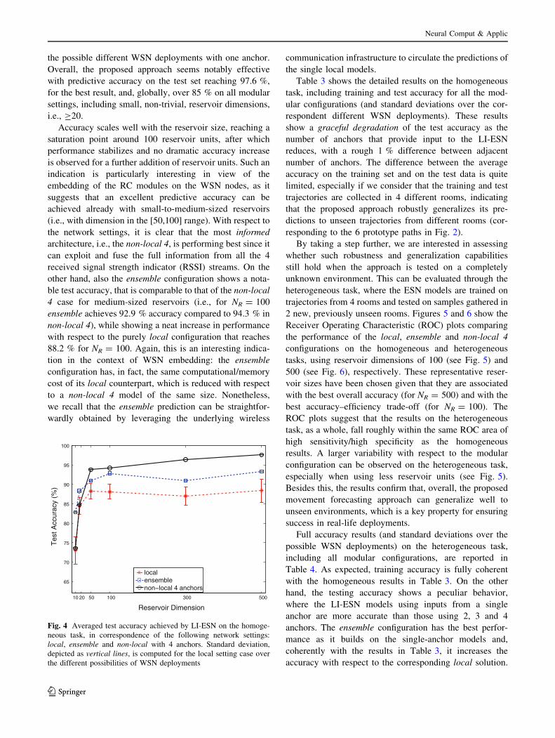
the possible different WSN deployments with one anchor.

Overall, the proposed approach seems notably effective

with predictive accuracy on the test set reaching 97.6 %,

for the best result, and, globally, over 85 % on all modular

settings, including small, non-trivial, reservoir dimensions,

i.e., C20.

Accuracy scales well with the reservoir size, reaching a

saturation point around 100 reservoir units, after which

performance stabilizes and no dramatic accuracy increase

is observed for a further addition of reservoir units. Such an

indication is particularly interesting in view of the

embedding of the RC modules on the WSN nodes, as it

suggests that an excellent predictive accuracy can be

achieved already with small-to-medium-sized reservoirs

(i.e., with dimension in the [50,100] range). With respect to

the network settings, it is clear that the most informed

architecture, i.e., the non-local 4, is performing best since it

can exploit and fuse the full information from all the 4

received signal strength indicator (RSSI) streams. On the

other hand, also the ensemble configuration shows a nota-

ble test accuracy, that is comparable to that of the non-local

4 case for medium-sized reservoirs (i.e., for NR = 100

ensemble achieves 92.9 % accuracy compared to 94.3 % in

non-local 4), while showing a neat increase in performance

with respect to the purely local configuration that reaches

88.2 % for NR = 100. Again, this is an interesting indica-

tion in the context of WSN embedding: the ensemble

configuration has, in fact, the same computational/memory

cost of its local counterpart, which is reduced with respect

to a non-local 4 model of the same size. Nonetheless,

we recall that the ensemble prediction can be straightfor-

wardly obtained by leveraging the underlying wireless

communication infrastructure to circulate the predictions of

the single local models.

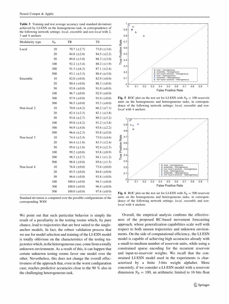
Table 3 shows the detailed results on the homogeneous

task, including training and test accuracy for all the mod-

ular configurations (and standard deviations over the cor-

respondent different WSN deployments). These results

show a graceful degradation of the test accuracy as the

number of anchors that provide input to the LI-ESN

reduces, with a rough 1 % difference between adjacent

number of anchors. The difference between the average

accuracy on the training set and on the test data is quite

limited, especially if we consider that the training and test

trajectories are collected in 4 different rooms, indicating

that the proposed approach robustly generalizes its pre-

dictions to unseen trajectories from different rooms (cor-

responding to the 6 prototype paths in Fig. 2).

By taking a step further, we are interested in assessing

whether such robustness and generalization capabilities

still hold when the approach is tested on a completely

unknown environment. This can be evaluated through the

heterogeneous task, where the ESN models are trained on

trajectories from 4 rooms and tested on samples gathered in

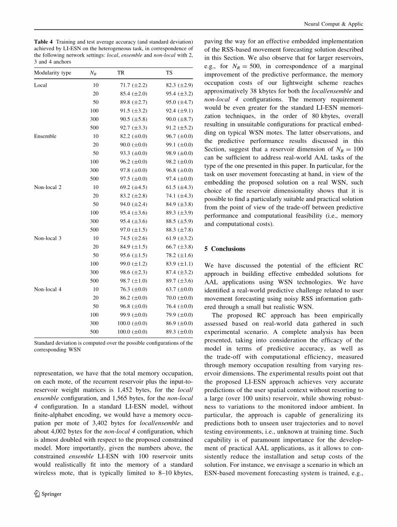
2 new, previously unseen rooms. Figures 5 and 6 show the

Receiver Operating Characteristic (ROC) plots comparing

the performance of the local, ensemble and non-local 4

configurations on the homogeneous and heterogeneous

tasks, using reservoir dimensions of 100 (see Fig. 5) and

500 (see Fig. 6), respectively. These representative reser-

voir sizes have been chosen given that they are associated

with the best overall accuracy (for NR = 500) and with the

best accuracy–efficiency trade-off (for NR = 100). The

ROC plots suggest that the results on the heterogeneous

task, as a whole, fall roughly within the same ROC area of

high sensitivity/high specificity as the homogeneous

results. A larger variability with respect to the modular

configuration can be observed on the heterogeneous task,

especially when using less reservoir units (see Fig. 5).

Besides this, the results confirm that, overall, the proposed

movement forecasting approach can generalize well to

unseen environments, which is a key property for ensuring

success in real-life deployments.

Full accuracy results (and standard deviations over the

possible WSN deployments) on the heterogeneous task,

including all modular configurations, are reported in

Table 4. As expected, training accuracy is fully coherent

with the homogeneous results in Table 3. On the other

hand, the testing accuracy shows a peculiar behavior,

where the LI-ESN models using inputs from a single

anchor are more accurate than those using 2, 3 and 4

anchors. The ensemble configuration has the best perfor-

mance as it builds on the single-anchor models and,

coherently with the results in Table 3, it increases the

accuracy with respect to the corresponding local solution.

10 20 50 100 300 500

65

70

75

80

85

90

95

100

Reservoir Dimension

Tes

t Acc

urac

y (%

)

localensemblenon−local 4 anchors

Fig. 4 Averaged test accuracy achieved by LI-ESN on the homoge-

neous task, in correspondence of the following network settings:

local, ensemble and non-local with 4 anchors. Standard deviation,

depicted as vertical lines, is computed for the local setting case over

the different possibilities of WSN deployments

Neural Comput & Applic

123

We point out that such particular behavior is simply the

result of a peculiarity in the testing rooms which, by pure

chance, lead to trajectories that are best suited to the single-

anchor models. In fact, the robust validation process that

we use for model selection and training of the LI-ESN model

is totally oblivious on the characteristics of the testing tra-

jectories which, in the heterogeneous case, come from a totally

unknown environment. As a result of this, it can happen that

certain unknown testing rooms favor one model over the

other. Nevertheless, this does not change the overall effec-

tiveness of the approach that, even in the worst configuration

case, reaches predictive accuracies close to the 90 % also in

the challenging heterogeneous task.

Overall, the empirical analysis confirms the effective-

ness of the proposed RC-based movement forecasting

approach, whose generalization capabilities scale well with

respect to both unseen trajectories and unknown environ-

ments. On the side of computational efficiency, the LI-ESN

model is capable of achieving high accuracies already with

a small-to-medium number of reservoir units, while using a

constrained sparse encoding for the recurrent reservoir

and input-to-reservoir weights. We recall that the con-

strained LI-ESN model used in the experiments is char-

acterized by a finite 3-bits weight alphabet. More

concretely, if we consider a LI-ESN model with a reservoir

dimension NR = 100, an arithmetic limited to 16 bits float

Table 3 Training and test average accuracy (and standard deviation)

achieved by LI-ESN on the homogeneous task, in correspondence of

the following network settings: local, ensemble and non-local with 2,

3 and 4 anchors

Modularity type NR TR TS

Local 10 70.7 (±2.7) 73.0 (±3.6)

20 84.8 (±2.6) 84.5 (±2.2)

50 89.8 (±3.0) 88.3 (±2.0)

100 92.2 (±3.4) 88.2 (±1.9)

300 91.3 (±6.3) 87.1 (±2.4)

500 93.1 (±3.3) 88.4 (±3.0)

Ensemble 10 82.0 (±0.0) 82.9 (±0.0)

20 90.4 (±0.0) 88.3 (±0.0)

50 93.8 (±0.0) 91.0 (±0.0)

100 96.7 (±0.0) 92.9 (±0.0)

300 97.9 (±0.0) 91.0 (±0.0)

500 96.5 (±0.0) 93.3 (±0.0)

Non-local 2 10 70.0 (±4.2) 66.2 (±7.1)

20 82.4 (±3.3) 82.1 (±3.8)

50 93.8 (±2.7) 89.2 (±3.2)

100 95.0 (±4.2) 91.2 (±3.8)

300 94.9 (±4.0) 93.6 (±2.2)

500 96.6 (±2.3) 93.8 (±5.0)

Non-local 3 10 74.4 (±2.4) 73.0 (±4.6)

20 84.4 (±1.8) 83.3 (±2.4)

50 95.6 (±1.6) 92.4 (±2.3)

100 99.2 (±0.8) 93.8 (±0.9)

300 98.3 (±2.7) 94.1 (±1.2)

500 98.8 (±0.8) 95.6 (±1.5)

Non-local 4 10 76.8 (±0.0) 73.6 (±0.0)

20 85.5 (±0.0) 84.8 (±0.0)

50 96.6 (±0.0) 93.8 (±0.0)

100 100.0 (±0.0) 94.3 (±0.0)

300 100.0 (±0.0) 96.4 (±0.0)

500 100.0 (±0.0) 97.6 (±0.0)

Standard deviation is computed over the possible configurations of the

corresponding WSN

0 0.1 0.2 0.3 0.4 0.5 0.6 0.7 0.8 0.9 10

0.1

0.2

0.3

0.4

0.5

0.6

0.7

0.8

0.9

1

False Positive Rate

Tru

e P

ositi

ve R

ate

local − homogeneousensemble − homogeneousnon−local 4 anchors − homogeneouslocal − heterogeneousensemble − heterogeneousnon−local 4 anchors − heterogeneous

Fig. 5 ROC plot on the test set for LI-ESN with NR = 100 reservoir

units on the homogeneous and heterogeneous tasks, in correspon-

dence of the following network settings: local, ensemble and non-local with 4 anchors

0 0.1 0.2 0.3 0.4 0.5 0.6 0.7 0.8 0.9 10

0.1

0.2

0.3

0.4

0.5

0.6

0.7

0.8

0.9

1

False Positive Rate

Tru

e P

ositi

ve R

ate

local − homogeneousensemble − homogeneousnon−local 4 anchors − homogeneouslocal − heterogeneousensemble − heterogeneousnon−local 4 anchors − heterogeneous

Fig. 6 ROC plot on the test set for LI-ESN with NR = 500 reservoir

units on the homogeneous and heterogeneous tasks, in correspon-

dence of the following network settings: local, ensemble and non-local with 4 anchors

Neural Comput & Applic

123

representation, we have that the total memory occupation,

on each mote, of the recurrent reservoir plus the input-to-

reservoir weight matrices is 1,452 bytes, for the local/

ensemble configuration, and 1,565 bytes, for the non-local

4 configuration. In a standard LI-ESN model, without

finite-alphabet encoding, we would have a memory occu-

pation per mote of 3,402 bytes for local/ensemble and

about 4,002 bytes for the non-local 4 configuration, which

is almost doubled with respect to the proposed constrained

model. More importantly, given the numbers above, the

constrained ensemble LI-ESN with 100 reservoir units

would realistically fit into the memory of a standard

wireless mote, that is typically limited to 8–10 kbytes,

paving the way for an effective embedded implementation

of the RSS-based movement forecasting solution described

in this Section. We also observe that for larger reservoirs,

e.g., for NR = 500, in correspondence of a marginal

improvement of the predictive performance, the memory

occupation costs of our lightweight scheme reaches

approximatively 38 kbytes for both the local/ensemble and

non-local 4 configurations. The memory requirement

would be even greater for the standard LI-ESN memori-

zation techniques, in the order of 80 kbytes, overall

resulting in unsuitable configurations for practical embed-

ding on typical WSN motes. The latter observations, and

the predictive performance results discussed in this

Section, suggest that a reservoir dimension of NR = 100

can be sufficient to address real-world AAL tasks of the

type of the one presented in this paper. In particular, for the

task on user movement forecasting at hand, in view of the

embedding the proposed solution on a real WSN, such

choice of the reservoir dimensionality shows that it is

possible to find a particularly suitable and practical solution

from the point of view of the trade-off between predictive

performance and computational feasibility (i.e., memory

and computational costs).

5 Conclusions

We have discussed the potential of the efficient RC

approach in building effective embedded solutions for

AAL applications using WSN technologies. We have

identified a real-world predictive challenge related to user

movement forecasting using noisy RSS information gath-

ered through a small but realistic WSN.

The proposed RC approach has been empirically

assessed based on real-world data gathered in such

experimental scenario. A complete analysis has been

presented, taking into consideration the efficacy of the

model in terms of predictive accuracy, as well as

the trade-off with computational efficiency, measured

through memory occupation resulting from varying res-

ervoir dimensions. The experimental results point out that

the proposed LI-ESN approach achieves very accurate

predictions of the user spatial context without resorting to

a large (over 100 units) reservoir, while showing robust-

ness to variations to the monitored indoor ambient. In

particular, the approach is capable of generalizing its

predictions both to unseen user trajectories and to novel

testing environments, i.e., unknown at training time. Such

capability is of paramount importance for the develop-

ment of practical AAL applications, as it allows to con-

sistently reduce the installation and setup costs of the

solution. For instance, we envisage a scenario in which an

ESN-based movement forecasting system is trained, e.g.,

Table 4 Training and test average accuracy (and standard deviation)

achieved by LI-ESN on the heterogeneous task, in correspondence of

the following network settings: local, ensemble and non-local with 2,

3 and 4 anchors

Modularity type NR TR TS

Local 10 71.7 (±2.2) 82.3 (±2.9)

20 85.4 (±2.0) 95.4 (±3.2)

50 89.8 (±2.7) 95.0 (±4.7)

100 91.5 (±3.2) 92.4 (±9.1)

300 90.5 (±5.8) 90.0 (±8.7)

500 92.7 (±3.3) 91.2 (±5.2)

Ensemble 10 82.2 (±0.0) 96.7 (±0.0)

20 90.0 (±0.0) 99.1 (±0.0)

50 93.3 (±0.0) 98.9 (±0.0)

100 96.2 (±0.0) 98.2 (±0.0)

300 97.8 (±0.0) 96.8 (±0.0)

500 97.5 (±0.0) 97.4 (±0.0)

Non-local 2 10 69.2 (±4.5) 61.5 (±4.3)

20 83.2 (±2.8) 74.1 (±4.3)

50 94.0 (±2.4) 84.9 (±3.8)

100 95.4 (±3.6) 89.3 (±3.9)

300 95.4 (±3.6) 88.5 (±5.9)

500 97.0 (±1.5) 88.3 (±7.8)

Non-local 3 10 74.5 (±2.6) 61.9 (±3.2)

20 84.9 (±1.5) 66.7 (±3.8)

50 95.6 (±1.5) 78.2 (±1.6)

100 99.0 (±1.2) 83.9 (±1.1)

300 98.6 (±2.3) 87.4 (±3.2)

500 98.7 (±1.0) 89.7 (±3.6)

Non-local 4 10 76.3 (±0.0) 63.7 (±0.0)

20 86.2 (±0.0) 70.0 (±0.0)

50 96.8 (±0.0) 76.4 (±0.0)

100 99.9 (±0.0) 79.9 (±0.0)

300 100.0 (±0.0) 86.9 (±0.0)

500 100.0 (±0.0) 89.3 (±0.0)

Standard deviation is computed over the possible configurations of the

corresponding WSN

Neural Comput & Applic

123

in laboratory/factory, on RSS measurements captured on

sample rooms and, then, deployed and put into operation

into its target environment, reducing the need for an

expensive configuration phase.

Further, we have proposed and empirically assessed

several modular architectures comprising single or multiple

RC modules with various degrees of mutual interaction,

from total independence to full RSS information sharing,

passing across intermediate ensemble-based architectures.

While full information sharing yields to the best overall

accuracy, the experimental results also point out the

effectiveness of an ensemble-based solution that comprises

RC modules performing independent predictions on sepa-

rate input information and weakly collaborating to achieve

a consensus prediction. Both modular configurations are

well suited to be deployed on a WSN, since the single LI-

ESN can be embedded into the motes and can interact

through the WSN communication service, either to share

RSS information or to achieve the consensus. In this

respect, the computational efficiency of the LI-ESN solu-

tion gains fundamental importance, given the resource-

constrained nature of WSN nodes and the reactivity

required to deliver timely predictions. To this end, partic-

ular care has been taken to define a parsimonious LI-ESN

model which builds on a sparse reservoir with a limited

number of units and a constrained weight alphabet,

strongly reducing the memory occupation due to the res-

ervoir, without significantly negatively impacting the pre-

dictive accuracy.

Overall, the results of the empirical analysis suggest that

LI-ESN has an excellent trade-off between accuracy,

generalization and efficiency, when dealing with noisy time

series data. As such, it can be considered a good candidate

for the development of a distributed learning system for

AAL applications that embeds the LI-ESN modules

directly on the wireless sensor nodes. As part of the

research effort of the EU FP7 RUBICON project, we plan

to develop such distributed learning infrastructure for

WSNs [5], founding on the LI-ESN approach discussed in

this paper. This learning system is intended to provide

adaptive movement forecasting and localization service in

WSNs, as well as more general event-recognition and

event-prediction services for AAL applications. Finally, as

a side contribution of this work, we have defined an

effective movement prediction benchmark, providing a

freely available dataset8 comprising extensive real-world

RSS measurements.

Acknowledgments This work is partially supported by the EU FP7

RUBICON project (http://www.fp7rubicon.eu/), Contract no. 269914.

References

1. AAL (2009) Ambient assisted living roadmap. http://www.

aaliance.eu/public/documents/aaliance-roadmap/

2. Antonelo EA, Schrauwen B, Campenhout JMV (2007) Genera-

tive modeling of autonomous robots and their environments using

reservoir computing. Neural Proc Lett 26(3):233–249

3. Antonelo EA, Schrauwen B, Stroobandt D (2008) Event detection

and localization for small mobile robots using reservoir com-

puting. Neural Netw 21(6):862–871

4. Bacciu D, Gallicchio C, Micheli A, Chessa S, Barsocchi P (2011)

Predicting user movements in heterogeneous indoor environ-

ments by reservoir computing. In: Bhatt M, Guesgen HW,

Augusto JC (eds) Proceedings of the IJCAI workshop on space,

time and ambient intelligence (STAMI) 2011, pp 1–6

5. Bacciu D, Chessa S, Gallicchio C, Lenzi A, Micheli A, Pelagatti

S (2012) A general purpose distributed learning model for robotic

ecologies. In: Robot Control—10th IFAC symposium on robot

control, vol 10(1), pp 435–440. doi:10.3182/20120905-3-HR-

2030.00178

6. Bahl P, Padmanabhan V (2000) RADAR: an in-building Rf-based

user location and tracking system. In: Proceedings of INFOCOM

2000. 19th Annual joint conference of the IEEE Comp. and

Comm. Soc. vol 2, pp 775–784. doi:10.1109/INFOCOM.2000.

832252

7. Barsocchi P, Lenzi S, Chessa S, Giunta G (2009) A novel

approach to indoor RSSI localization by automatic calibration of

the wireless propagation model. In: IEEE 69th vehicular Tech.

Conf., pp 1–5. doi:10.1109/VETECS.2009.5073315

8. Barsocchi P, Lenzi S, Chessa S, Giunta G (2009) Virtual cali-

bration for RSSI-based indoor localization with IEEE 802.15.4.

In: 2009 IEEE international conference on Comm. ICC ’09,

pp 1–5. doi:10.1109/ICC.2009.5199566

9. Battiti R, Villani A, Le Nhat T (2002) Neural network models for

intelligent networks: deriving the location from signal patterns.

In: Proceedings of AINS2002, Citeseer

10. Boedecker J, Obst O, Mayer N, Asada M (2009) Initialization and

self-organized optimization of recurrent neural network connec-

tivity. HFSP J 3(5):340–349

11. Brunato M, Battiti R (2005) Statistical learning theory for loca-

tion fingerprinting in wireless LANs. Comput Netw ISDN Syst

47(6):825–845. doi:10.1016/j.comnet.2004.09.004

12. Busing L, Schrauwen B, Legenstein R (2009) Connectivity,

dynamics, and memory in reservoir computing with binary and

analog neurons. Neural Comput Appl 22(5):1272–1311

13. Chang M, Terzis A, Bonnet P (2009) Mote-based online anomaly

detection using echo state networks. In: Krishnamachari B, Suri

S, Heinzelman W, Mitra U (eds) Distributed computing in sensor

systems, lecture notes in computer science, vol 5516. Springer,

Berlin, pp 72–86

14. EvAAL (2011) The 1st evaal competition, evaluating aal systems

through competitive benchmarking. Special theme on Indoor

Localization and Tracking, AAL Forum proceedings, valencia,

ES

15. Fette G, Eggert J (2005) Short term memory and pattern matching

with simple echo state networks. In: Proceedings of the international

conference on artificial neural networks (ICANN), Springer,

Lecture Notes in Computer Science, vol 3696, pp 13–18

16. Gallicchio C, Micheli A (2010) A markovian characterization of

redundancy in echo state networks by PCA. In: Proceedings of

the European symposium on artificial neural networks (ESANN)

2010, d-side, pp 321–326

17. Gallicchio C, Micheli A (2011) Architectural and markovian

factors of echo state networks. Neural Netw 24(5):440–456.

doi:10.1016/j.neunet.2011.02.0028 http://wnlab.isti.cnr.it/paolo/index.php/dataset/6rooms.

Neural Comput & Applic

123

18. Gallicchio C, Micheli A, Barsocchi P, Chessa S (2012) User

movements forecasting by reservoir computing using signal

streams produced by mote-class sensors. In: Mobile lightweight

wireless systems (Mobilight 2011), lecture notes of the institute

for computer sciences, social informatics and telecommuni-

cations engineering, vol 81. Springer, Berlin, pp 151–168.

doi:10.1007/978-3-642-29479-2_12

19. Gartner T (2003) A survey of kernels for structured data. SIG-

KDD Explor Newsl 5:49–58

20. Hajnal M, Lorincz A (2006) Critical echo state networks. In:

Proceedings of the international conference on artificial neural

networks (ICANN) 2006, pp 658–667

21. Hartland C, Bredeche N (2007) Using echo state networks for

robot navigation behavior acquisition. In: IEEE international

conference on robotics and biomimetics, IEEE, pp 201–206

22. Jaeger H (2001) The ‘‘echo state’’ approach to analysing and

training recurrent neural networks. Tech. rep., GMD—German

National Research Institute for Computer Science

23. Jaeger H, Haas H (2004) Harnessing nonlinearity: predicting

chaotic systems and saving energy in wireless communication.

Sci Agric 304(5667):78–80

24. Jaeger H, Lukosevicius M, Popovici D, Siewert U (2007) Opti-

mization and applications of echo state networks with leaky-

integrator neurons. Neural Netw 20(3):335–352

25. Kolen J, Kremer S (eds) (2001) A field guide to dynamical

recurrent networks. IEEE Press, Parsippany

26. Kontkanen P, Myllymaki P, Roos T, Tirri H, Valtonen K, Wettig

H (2004) Topics in probabilistic location estimation in wireless

networks. In: Personal, indoor and mobile radio communications,

2004. PIMRC 2004. 15th IEEE International Symposium on, vol

2, pp 1052–1056. doi:10.1109/PIMRC.2004.1373859

27. Kushki A, Plataniotis K, Venetsanopoulos AN (2007) Kernel-

based positioning in wireless local area networks. IEEE Trans

Mobile Comp 6(6):689–705. doi:10.1109/TMC.2007.1017

28. Legenstein RA, Maass W (2007) Edge of chaos and prediction of

computational performance for neural circuit models. Neural

Netw 20(3):323–334

29. Liu H, Darabi H, Banerjee P, Liu J (2007) Survey of wireless

indoor positioning techniques and systems. Systems, man, and

cybernetics, part C: applications and reviews. IEEE Trans

37(6):1067–1080. doi:10.1109/TSMCC.2007.905750

30. Lukosevicius M, Jaeger H (2009) Reservoir computing approa-

ches to recurrent neural network training. Comput Sci Rev

3(3):127–149

31. Luo X, OBrien WJ, Julien CL (2011) Comparative evaluation of

received signal-strength index (RSSI) based indoor localization

techniques for construction jobsites. Adv Eng Inf 25(2):355–363

32. Maass W, Natschlager T, Markram H (2002) Real-time com-

puting without stable states: a new framework for neural

computation based on perturbations. Neural Comput 14(11):2531–

2560. doi:10.1162/089976602760407955

33. Obst O (2009) Distributed fault detection in sensor networks

using a recurrent neural network. Tech. rep., CoRR, abs/0906.

4154

34. Oubbati M, Kord B, Palm G (2010) Learning robot-environment

interaction using echo state networks. In: Proceedings of the 11th

international conference on Simul. of adapt. behavior, Springer-

Verlag, SAB’10, pp 501–510

35. Pan JJ, Kwok J, Yang Q, Chen Y (2006) Multidimensional vector

regression for accurate and low-cost location estimation in per-

vasive computing. IEEE Tran Knowl Data Eng 18(9):1181–1193.

doi:10.1109/TKDE.2006.145

36. Rodan A, Tino P (2011) Minimum complexity echo state net-

work. IEEE Trans Neural Netw 22(1):131 –144

37. Steil JJ (2004) Backpropagation-decorrelation: online recurrent

learning with O(N) complexity. In: Proceedings of the IEEE

international joint conference on neural networks (IJCNN) 2004,

vol 2, pp 843–848

38. Steil JJ (2006) Online stability of backpropagation-decorrelation

recurrent learning. Neurocomputing 69(7–9):642–650

39. Tino P, Dorffner G (2001) Predicting the future of discrete

sequences from fractal representations of the past. Mach Learn

45(2):187–217

40. Tino P, Cernansky M, Benuskova L (2004) Markovian archi-

tectural bias of recurrent neural networks. IEEE Trans Neural

Netw 15(1):6–15

41. Verstraeten D, Schrauwen B, D’Haene M, Stroobandt D (2007)

An experimental unification of reservoir computing methods.

Neural Netw 20(3):391–403

42. Waegeman T, Antonelo E, Wyffels F, Schrauwen B (2009)

Modular reservoir computing networks for imitation learning of

multiple robot behaviors. In: 8th IEEE international symposium

on comput. intelligence in robotics and autom., IEEE, pp 27–32

43. Wu CL, Fu LC, Lian FL (2004) Wlan location determination in

e-home via support vector classification. In: Networking, sensing

and control, 2004 IEEE international conference on, vol 2,

pp 1026–1031

44. Youssef M, Agrawala A (2005) The horus WLAN location

determination system. In: MobiSys’05: proceedings of the 3rd

international conference on mobile Sys. appl. and services. ACM,

New York, pp 205–218. doi:10.1145/1067170.1067193

45. Zaruba GV, Huber M, Kamangar FA, Chlamtac I (2007) Indoor

location tracking using RSSI readings from a single wi-fi access

point. Wireless Netw 13:221,235

Neural Comput & Applic

123