T .;\yCf.' i/^:-'

AN EXPANSION THEOREM FOR A CLASS OF

NON-SELF-ADJOINT BOUNDARY

VALUE PROBLEMS

by

JOHN COLMAN DRUMMOND, JR., B.S.

A THESIS

IN

MATHEMATICS

Submitted to the Graduate Faculty of Texas Technological College

in Partial Fulfillment of the Requirements for

the Degree of

MASTER OF SCIENCE

Approved

Accepted

August 1968

J05 / 0

\<^loi

Ho.

Cof-

lid

X

ACKNOWLEDGEMENTS

I would like to express my appreciation to Dr. Ronald

M. Anderson for his direction of this thesis. I would also

like to thank the other members of my committee. Dr. Patrick

L. Ode11 and Dr. John T. White.

11

TABLE OF CONTENTS

LIST OF ILLUSTRATIONS iv

INTRODUCTION 1

CHAPTER

I. Some'Preliminary Lemmas 3

II. The Expansion Theorem 25

III. Two Examples 40

LIST OF REFERENCES 48

111

LIST OF ILLUSTRATIONS

Figure

1. Path of Contour Integration -No Poles on Real Axis 26

2. Path of Contour Integration -Simple Poles on the Real Axis 38

IV

INTRODUCTION

In his Ph.D. dissertation, Donald Cohen develops the

expansion formula associated with the following non-self-

adjoint boundary value problem

y" (x) + s^ y (x) = 0 0 <_ x < °o

y' (0) + D y(0) = 0

lim |y'(x) - is y(x)| = 0

where D is a complex constant and Im s > 0. Cohen's expan­

sion theorem is for the class of functions f(x) which are

continuous, have piecewise continuous first and second

derivatives in x >_ 0 and that

f" (x) = 0 (x"^) as x->oo

f (x) = 0 (x ) as x-oo

The purpose of this paper is to extend the above expan­

sion formula to a more general class of non-self-adjoint

boundary value problems. We will consider the system:

y" (x) + (s - q(x))y(x) = 0 0 £ x < oo

y' (0) + Dy (0) = 0

lim |y(x) - e | = 0 x->°°

Where D is a complex constant and Im s >_ - -j for some 6 > 0.

Furthermore q(x) must satisfy the following conditions:

(i) q(x) e C[0,~)

(ii) e / ^q(x) e L[0,c») for the same

6 as above

In order to obtain an expansion theorem we impose the fol­

lowing conditions on f(x)

(i) f(x) z C^[0,c»)

(ii) f(x) e L^[0,~)

(iii) f" (x) = 0(x"^) as x-oo

In chapter two, existence theorems and formulas are

developed for a solution of the differential equation which

satisfies the boundary conditions at zero and for a solu­

tion which satisfies the boundary condition at infinity.

Asymptotic expansions are also developed for these solutions

and for the wronskian of these solutions for large values

of |s

The expansion theorem is stated and proven in chapter

three and chapter four contains two examples. The first

example is the same as Cohen's problem, i.e. q(x) E 0.

2 ~x/o. In the second example we take q(x) = -3 e ^ , where 3eR

and a > 0.

Chapter I

SOME PRELIMINARY LEMMAS

In order to prove the expansion theorem in chapter

three the following lemmas are needed. Lemmas one and

three prove the existence of solutions to the differential

equation which satisfy the prescribed boundary conditions.

These solutions are set up as solutions of integral equa­

tions. Asymptotic expansions, for large values of |s|, for

these solutions and their derivatives are developed in

lemmas two, four, five and six. The asymptotic expansion

for the wronskian is developed in lemma seven and lemma

eight gives the asymptotic expansion for the inverse of

the wronskian.

Lemma 1: Consider the system

(1.1) v"(x) + (s^ - q(x))v(x) = 0 0 £ X < 00

(1.2) V' (0) = -D

(1.3) v(0) = 1

where q (x) e C [0,oo) , e^^ ^ | q ( y ) |dy < oofor some 6 > 0 J

and Im s > - 6 / 4 .

This system has a unique solution and if(|)(x) = (^{x,s)

is the solution then we can write ( (x,s) as

X

(1 .4 ) <^{x,s) = cos sx - iiiL_12i D + 1/s s i n s (x-y) q (y) ( (y , s ) d y . {)

Furthermore, (})(x,s) is an entire function of s.

Proof: From the basic existence and uniqueness theorems

such as in [21, we know that the above system has a unique

solution on (-00,00) and hence on [0,oo).

Let ({) (x) = (j)(x,s) be this solution. Then (^{x,s) e C[0,oo)

as a function of x. Also sin s (x-y) and q(y) are both con­

tinuous functions of y for y e [0," ) and so the integral

X

sin s (x-y)q(y)^(y,s)dy

0 exists for all x >_ 0. Therefore, the right-hand side of (1.4)

is well-defined. We also have:

X

1/s sin s (x-y)q(y)i(y,s)dy =

0

1/s sin s (x-y) [({)" (y ,s)+s c{)(y,s)]dy

0

where y = — ^(x,s). Breaking the integral on the right a X

into two integrals and integrating the first of these twice

by parts, we get: X

1/s sin s (x-y)q(y) (}) (y,s)dy = -1/s sin sX(|)'(0,s)

X

+ 4,(x,s)-cos sx (f)(0,s) -s sin s (x-y) (^ (y ,s)dy

+ s sin s (x-y) (J) (y ,s)dy = D/s sin sx -cos sx + <^{x,s)

Therefore

sin sx ^ , ^ , cos sx - D + 1/s sin s (x-y)q (y) (|> (y ,s)dy = <^{x,s)

Hence, any solution of (1.1) which satisfies (1.2) and (1.3)

can be written as (1.4)

The analyticity of (j)(x,s) follows from theorems 5.2

and 8.4 in chapter on of [2].

Lemma 2: Let '(^{x,s) be the solution of (1.1) which satisfies

(1.2) and (1.3). Then

Itlx (f)(x,s) = COS sx + 0 (—I—\—) as |s|->°° and

Im s = t > -6/4.

This result holds uniformly for x e [0,°°).

Proof: Let Im s = t and consider a function F(x,s) defined

as :

F (x, s) = e ' I (|) (x, s)

From lemma 1 we know that (|)(x,s) has the form (1.4) and so

F(x,s) becomes

T / \ "|t|x -|t|x sin sx ^ F(x,s) = e ' ' cos sx - e ' ' D

f - I t I X 111 v + 1/s sin s(x-y)q(y)e ' ' e' ' F(y,s)dy

•

0

which implies

—Itlx -jtlxi F(x,s) I <_ |cos sx I e ' ' + |sin sx | e ' ' |D/s|

sin s(x-y) I |q(y)F(y,s) I e" ' ' """ ^ ^ . ' -

s I 0

But

COS sx| < 1/2(e 1^'^ + e'^'^)

sin sxl < 1/2 (e l^'^ + el" ! )

and substituting we get

(1.5) |F(x,s)| <_ l/2(e-2|t|x+ i) + i/2(e"2|t|x^ ^ D/s

2 s (^-2|t|(x-y)^ 1) |q(y)F(y,s) dy

0 X

< 1 + ID/sI + q(y) I |F(y,s) Idy

0 -Itlx Both (|)(x,s) and e i^i" are continuous functions of x for

x ^ 0 and so F(x,s) is continuous for x > 0 and so for any

X > 0

max |F(y,s) 0<y<x

= M < 00

X

Combining this with (1.5) we get:

X

M^ <_ 1 + |D/s| + 1 |q(y) |M^dy

< 1 + ID/sI + |q(y) I M dy

which implies

M [1 -X ' IS

q(y)| dy] < 1 + |D/s

0 Now pick SQ such that if |s| > SQ, then

00

|q(y) |dy < 1

and hence 00

1 - q(y)Idy > 0

and we get

M

0

1 + ID/s 1 + |D/sn X —

1 - q (y) |dy 1 - 1/s 0 q(y)|dy

0 0

for |s| > SQ .

But X was arbitrary and the right-hand side of the above

expression is independent of x and so we get

F(x,s) I < 1 + ID/s 0

,00

1 - 1/s 0 q(y) |dy

for all X >_ 0

and |s'| > s^

0

Hence, F(x,s) = 0(1) as s ->oo

Itlx 11 X and so 4)(x,s) = e' ' F(x,s) = 0(e' ' )

as s ->oo

Then

(f) (x,s) - cos sx| <_

X

ism sx D + sin s(x-y)IIq(y)

0

(f) (y/S) |dy

and for |s| > S Q , we get:

({) (x,s) - cos sx < 1 [i/2(e l^l^+el^l'') ID

X

+ A/2 f (e-|t|(x-y)^Jt|(x-y), ^^^, |t|y^^

8

where A is the 0-constant for <^{x,s). Then

X {^ ^\ I 1 r D / - t X. t X,

(J)(x,s) - COS sx < -i—r [- r (e ' I + e' ' ) — s

+ A/2 ^^/^~ 111 (x-2y) , |t|Xv| / vi-i T (e ' 1 ' - + e I 1 ) q (y) dy]

0 t |x r 00

[ iDl + A t |x ,00

q(y)|dy] £ el^lil [|D|+A |q(y)|dy]

0 0

Hence

(j)(x,s) - cos sx = 0(^-1—1—) as |s|->oo

and so

(x,s) = cos sx + 0(—I— \—) as s U-oo

This result is uniform in x since the choice of s 0

does not depend on x.

Lemma 3: Consider (1.1) with the boundary condition

(1.6) lim |v(x) - e X->oo

ISX = 0

where q(x) e C[0,oo),

and Im s = t > -6/4.

^ \q{x) |dx < 00 for some 6 > 0

0

This system has a solution and at least one solution

can be written as:

isx (1.7) 4'(x,s) = e + 1/s sin s (y-x)q (y)'i'(y ,s) dy

0 Furthermore, m{x,s), as written above, is an analytic

function of s for Im s > - 6/4.

Proof: Consider the integral equation

(1.8) h(x,s) = 1 -2is

(1 - e 2is(y ^))q(y) h(y,s)dy

X

We can solve this equation by the method of succession

approximations. Let

9

h^(x,s) = 1

h (x,s) = 1 n 2is

(1 _ e^^^^^ ''^)q(y) h^_^(y,s)dy

Note that:

(i) h^ is well-defined for all x and s.

(ii) |hj^(x,s) I <. 1 + r ,1 - e

2is (y-x)

2is |q(y) |dy

X

But

1 - e 2is (y-x)

2is

x-y x-y -2lS-r-, I

e ^dx < :2tM,

0 0

and /

x-y e d-c <

x-y if t > 0

< <

0 V x-y e

2(x-y)t if -6/4 < t < 0 for y>x

Then if t > 0:

1 + x-y I |q (y) |g (y)dy <. 1 + x-y I e -^/2y|q(y)|e^/2yg(y)dy

X X

< 1 + ( ( y - x ) V % y ) l / 2 ( / N |2 6y 2, . . .1/2 q (y) e - g (y)dy)

X x

10

which exists if g (y) is bounded and continuous for y e [0,co)

If t < 0:

1 + x-y|e^^^ ^^^|q(y) |g(y)dy

X

< 1 +

< 1 +

X

< 1 + (

fv-vlo2(>^-y)t-6/2 y^6/2 y, ... ... ly-xje -" -^ e ' -^ |q(y) |g(y)dy

fv-v^^(-2t-V2) (y-x) 6/2 y, , . , . .. ^y-x;e -" e |q(y)|g(y)dy 00

(y-x)V/2(-4t-6)(y-x)^^^l/2j

Y ( \ ^<5y, , X ,2 2 , , . ,1/2 X ( e ^ |q (y). | g (y)dy) ^

X

which exists if g(y) is bounded and continuous for y e [0, )

(since -4t -6 <0)

Then, with g(y) E 1 we have

|h^(x,s) I £ 1 + M( e^^|q(y) | dy) 6y 2. ,1/2

where M = max (sup ( (y-x) e ^dy) ^ , sup X

X

, ,2 l/2(-4t-6)(y-x) , xl/2, . , , (y-x) e ^ "'- M y ) ^ } and so h^(x,s) is well-

defined for all X and for all s such that Im s > - 6/4.

(iii) Assume

hj^(x,s) I <_ 1 + M( 6y e<^^|q(y) | dy) 2^„^l/2

+ • • • + M

x k

/k J X

([ e«y|q(y)|2dy)'^/2

Then

11

hj^(x,s) I <_ 1 + 1 - e 2is (y-x)

< 1 + 1 - e

X

2is (y-x)

2is q(y) I l\(y/s) |dy

X 2is

q (y) |dy + I l_e2is(y-x)

J X

2is

q(y) |M( e'^^lq(z) |^dz)^/^dy J y

+ .. .+ f ,1 - e^^^^^~^^

2is q(y)

M

/k

6z I , X I 2, xk/2, : q (z) dz) ^ dy

And Using the same reasoning as in (ii) we get:

|h (x,s) I £ 1 + M(f e'5^|q(y) l^dy)^/^

+ M ( e^^|q(y)|^( e* ^ |q(z) |^dz)dy)-'-/^ +• • • +

X

+ ^-k+1 r

- (

/k

= 1 + M(

6y I / X 12 , ^ q(y) (

6z I , X ,2. ,k. ,1/2 e q (z) dz) dy)

X

e^^ |q(y) I dy)

y

2. ,1/2

X

+ M 2 ( ^ ^ dy k+l\

6z I , X ,2, xk+1^ ,1/2 e q (z) dz) dy)

+ • . • +

X V , _ 00 J oo

-.k+1 r -, -, r M , /k dy k+1

6z , , X 12-, ,k+lj , 1/2 e"" q (z) dz) dy)

= 1 + M( 6y 2^„,l/2 _, M 2 ;

q(y) I dy) ^ + — ( /2 J

6y I / \I 2, ,1 e ^ q(y) dy)

X

12

M k+1

~ (

/k+T J

k+1

e^^ |q(y)l^dy) 2 00 m »-K

Y M L

(

n=0 » k J

^6y I , X ,2. ,k/2 e q(y) dy)

X --- - 0

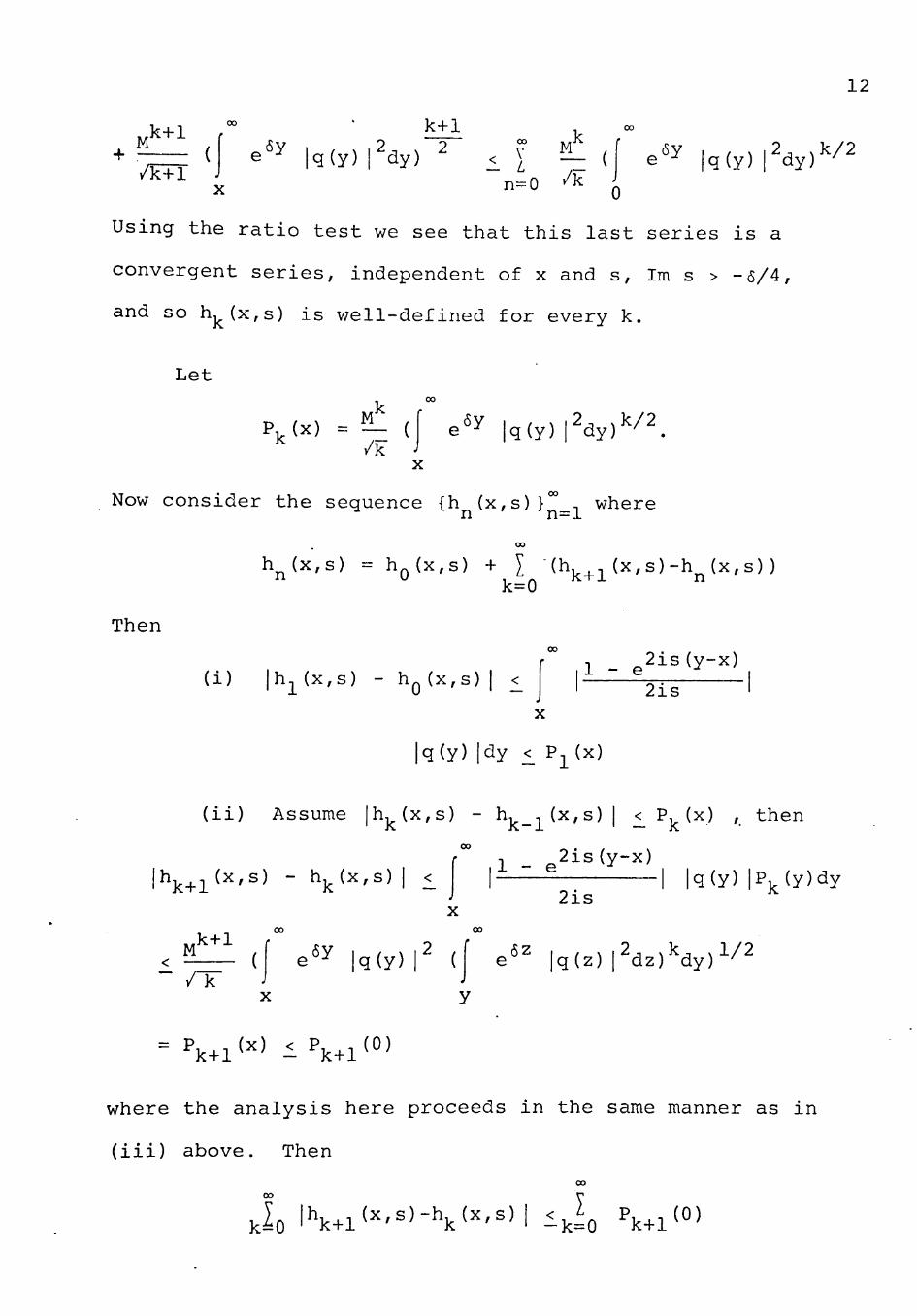
Using the ratio test we see that this last series is a

convergent series, independent of x and s, Im s > -6/4,

and so hj^(x,s) is well-defined for every k.

Let

P^(x) = M

/k J

^<5y I , X ,2-, , k / 2 e q(y) dy)

X

Now consider the sequence {h (x,s)}°° , where ^ n ' n=l

Then

h^(x,s) =hQ(x,s) + \ "(hj^^^(x,s)-h^(x,s) ) k=0

(i) \\\^ (x,s) - h^ (x,s) I <_ •°° 1 _ g2is(y-x)

2is

|q(y) |dy <_ P^ (x)

(ii) Assume |hj (x,s) - h,_,(x,s)| £ P, (x) , then

" 1 - e^^^^^"^^ \ + l ^^'^^ ~ hj^(^^s) I <

X 2is

q(y) |Pk(y)dy

M k+1

/IT 6 y I / \ 1 2 /

e q (y) ( e* ^ |q(z) |^dz)^dy)^/^

X

= ^+i"^) ^ ^ + i ' ° '

where the analysis here proceeds in the same manner as in

(iii) above. Then

klo l\+i(^'S)-h^(x 'S)| ±1 k=0 ^+1'°'

13

which is convergent and so

00

hQ(x,s) + I |\+i(^'S) - hj^(x,s)|

is uniformly convergent for all x e [0,oo) and for all s

such that Im s > -6/4. Let h(x,s) be the limit function

Then

lim h (x,s) = h(x,s) uniformly in x and s. X->-00

Then

h(x,s) lim h (x,s) V n '

= lim [1 -X-x 2is

(1 - e 2is (y-x).

X

q(y) h^_i(y/S)dy]

But h (x, s)->h (x, s) uniformly implies

1 2is

2is (v—x) (1 - e - )q(y) h _, (y,s)dy converges to

X

2is X

2 i s (V—X) (1 - e - )q(y) h(y,s)dy uniformly in x and

s where Im s > -6/4

Hence

h(x,s) = 1 -2is

(1 - e J X

2is (y-x), / X, , X , ^ )q(y)h(y,s)dy

and so the integral equation (1.8) has a solution.

We also have that

lim e* / |h(x,s)-l| = 0 X->-oo

14

since

^6/2 X h(x,s)-l I < e 6/2 X 1 - e

2is (y-x)

2is

q(y)I|h(y,s) Idy

and given any e > 0 there exists an N such that

h^(x,s) - h (x,s) I < e for n > N

which implies

h(x,s) I < e + Ih (x,s) I < e + y P, (0) for n > N,

Hence

and so we get

h(x,s) < I P, (0) ~k=0 ^

6/2 |, , , T , 6/2 X e ' h (x,s)-1 < e '

f* 1 _ ^2is(y-k) 1 - e

X 2is

|q(y) I I P, (0)dy k=0

Then if t > 0:

<5/2|, / X T I 6/2 X e ^ h (x,s)-1 < e ' I* 00

X

/ N -<5/2 y^6/2 y , , (y-x) e ' ^e ' q(y)

X I P, (0)dy k=0

X < M(

(y-x)e^/2(x-y)^6/2 y ^^^^^ j

k=0 00

e^^ | q ( y ) | ^ I P, (0))2dy)l/2

k=0 ^

X k=0

15

where M is defined as before. But

and e^^ ^ q(y) e C[0,oo) implies

f V2 y , X . e -^q(y)dy < 00

0

, 00

e^^ |q(y) l dy < 00

0

and so we can pick x^ such that for x > x^

6y

x Then, for x > x

|q(y) \U I P, (0))^dy < e . k=0

0

e^/^ ^ |h(x,s)-l| < M .£ .

Now if t < 0:

6/2 X |, , , , , 6/2 X e ' h (x,s)-1 < e f°°

X

, , -2t(y-x)-6/2 yi , (y-x)e J' ' / J |q(y

x

il Pj^(0))dy k=0

, , (-2t-6/2) (y-x) 6/2y /-x /^ r, /A ^ (y-x)e' / / J' 'e / - q(y) ( Pj (0))dy k=0

< M( e^^ |q(y) | ( I Pj^(0))dy^/^ k=0

and as above, for x > x^, we get:

*^/^ ^ | h ( x , s ) - l | < M-e.

Hence

l i m e*^/^ ^ | h ( x , s ) - l | = 0 . X->oo

— isx Nov;, if we write h(x,s)=e H'(x,s)we get

16

-isx (x,s) = 1 (.00

2is (1 - e"

2is (y-x), , , -isy , ,. '- ')q(y)e ^<i/(y,s)dy

X

which implies

1'(x,s) = e^^"" + i s

,oo

sin s (y-x)q (y) H* (y,s)dy

X

and so (1.7) has a solution. Also note that, since

sin s (y-x)q (y)^(y,s)dy

X

and 0

cos s (y-x) q (y) H* (y , s) dy

•0 both converge uniformly for x _> 0, we may differentiate under

the integral sign with respect to x [1]. We get:

4*' (x,s) = ise ISX cos s (y-x)q (y) H'(y,s)dy

X

and

H' (x,s) = -s e - s sin s (y-x)q (y) H'(y,s)dy

X

and so

^" (x,s) + (s'^-q(x))^(x,s) = 0

That is, the solution of (1.7) is also a solution of (1.1).

Note that y(x,s) also satisfies 1.6:

lim YI(x,s) X-^oo

- e ISX = lim Ie I Ih(x,s)-1

x->°°

lim e Ih (x,s)-1 X->oo

T . (-t-6/2)x 6/2 X 1^, , . = lim e ' ' e ' |h(x,s)-l = 0

x->°°

17

• We now show that H'(x,s), as expressed in (1.7), is an

analytic function of s for Im s > -6/4. In the following

discussion, "f(x,s) is analytic" will mean that f(x,s) is

an analytic function of s for Im s > -6/4.

From the first part of this proof we have that

h^(x,s)->h(x,s)

uniformly for all s such that Im s > -6/4, and hence, the

convergence is normal in s for Im s > -6/4.

Consider the function

1 _ g2is(y-ic) g(x,y,s) = 2ii q ^

It is an entire function of s. We also have that

h^(x,s) = 1

is an entire function. Assume h, _, (x,s) is an analytic func­

tion and consider

(1.9) g(x,y,s)hj^_^(y,s)dy

This is an analytic function since g(x,y,s) and h,_,(y,s)

are both analytic functions [4]. We also have that (1.9)

converges uniformly, and hence,' normally, to

rb (1.10) g(x,y,s)hj^_^(y,s)dy

x

for all s such that Im s > -6/4. Therefore (1.10) is an

analytic function [4] and so

18

h, (x,s) = 1 - g(x,y,s)hj^_^(y,s)dy

X

is an analytic function.

As was noted above, h (x,s) converges normally to

h(x,s), but each h (x,s) is analytic, and so h(x,s) is

ISX, analytic [4]. But H'(x,s) = e h(x,s) and since e ISX . IS

an entire function and h(x,s) an analytic function, then

H'(x,s) must be an analytic function. That is, m {x,s) is

an analytic function of s for Im s > -6/4.

This completes the proof of lemma 3.

Lemma 4: Let 'i'(x,s) be the solution of (1.1) which satisfies

(1.6) and has the form of (1.7). Then

m (x,s) = e + 0 (— - I t l x

) as |s|->oo for Im s = t > -6/4

Proof: Let h (x,s) be as in lemma 3. Then h (x,s) converges n n ^

uniformly to h(x,s) for all x ^ 0 and for all s such that

Im s > -6/4. Hence, given any e > 0 there exists an N such

that for n > N

|h (x,s) I - |h^(x,s) <_ |h (x,s)-h^(x,s) I < e

which implies

h (x,s) I < e + |h^(x,s)

But

k=0

19

and so 00

h ( x , s ) I ^ I Pj^(O) k=0

Then

f°°,l - e^^^^^"^^ 2Ti 1 | q ( y ) I | h ( y , s ) | d y £ 1 - e 2 i s ( y - x )

2 is q(y)

X

X I Pj^(0)dy k=0

- V -D /' > 1 f / - 6 / 2 y , - 2 t ( y - x ) - 6 / 2 y , 6 /2 y , , x i -, - 2. ^ k ^ ^ 2 i n ^^ " ^ ^ ^ | q ( y ) | d y

k=0 X

k=0

5/2 y

X

q ( y ) | d y £ j ; P ^ (0) - i - e * ^ ^ |q (y) |dy k=0 ' ' ^

which implies

and so

h(x,s) = 1 + O(-Ai-) I o I

I* (x, s) = e + 0 (—

as I s I ->oo for

Im s = t > -6/4

t X -) since

ISX ^ / 1 , I e O (i—r) < s

s ' '

-tx A el I ( ^(-t-|t|)x, ^ e_ X

' A

as s ->-oo

which implies

e^-^ 0(-^) = 0 ( ^ ) as s ->-oo

Lemma 5: Let (t)(x,s) be the solution of (1.1) which satisfies

(1.2) and (1.3). Then

20

( | ) ' (x , s ) = - s s i n sx + 0 ( e ' ^ ' ^ )

and where 4)' ( x , s ) = ~ <^ ( x , s ) .

o X

Proof: From lemma 1 we have

(|)(x,s) = cos sx - D/s sin sx + 1/s

which implies [1] :

as I s I ->«> for

Im s = t > -6/4,

X sin s (x-y)q(y) ({) (y,s)dy

0

(() ' (x,s) + s sin sx - D cos sx +

Then

X cos s (x-y)q (y) (|) (y ,s)dy .

0

(|) ' (x,s) + s sin sxl < IDI ICOS SX

fX [COS S (x-y) I |q (y) I I 4) (y ,S) |dy

But from lemma 2 we have 4)(y,s) = 0 (e' 1 ) and so for

0

s I > Sj we get

. I / \ , • I |D / t X •- t X, (f) ' (x,s) + s s m sx| <_ II (e' ' +e ' ' )

+ A/2 '^ , |t|(x-y)^ -|t|(x-y), Itly, , , (el ' - +e ' I - ) e I ' |q (y) dy

0

= el^l^ [1^(1 + e-2|t|^) + A/2 rX II

(1 + e"2|^l ^^-y))|q(y)|dy]

|t|x r Ir

< e' ' [ D

rx [ p + A |q(y) |dy]

0

where A is the 0-constant for (f)(y,s).

t X, Hence, 4)' (x,s) = - s sin sx + 0(e' " ' ' " ) . as | s |-°° for

Im s = t > -6/4.

Lemma 6: Let (x,s) be the solution of (1.1) which satisfies

(1.6) and has the form of (1.7). Then

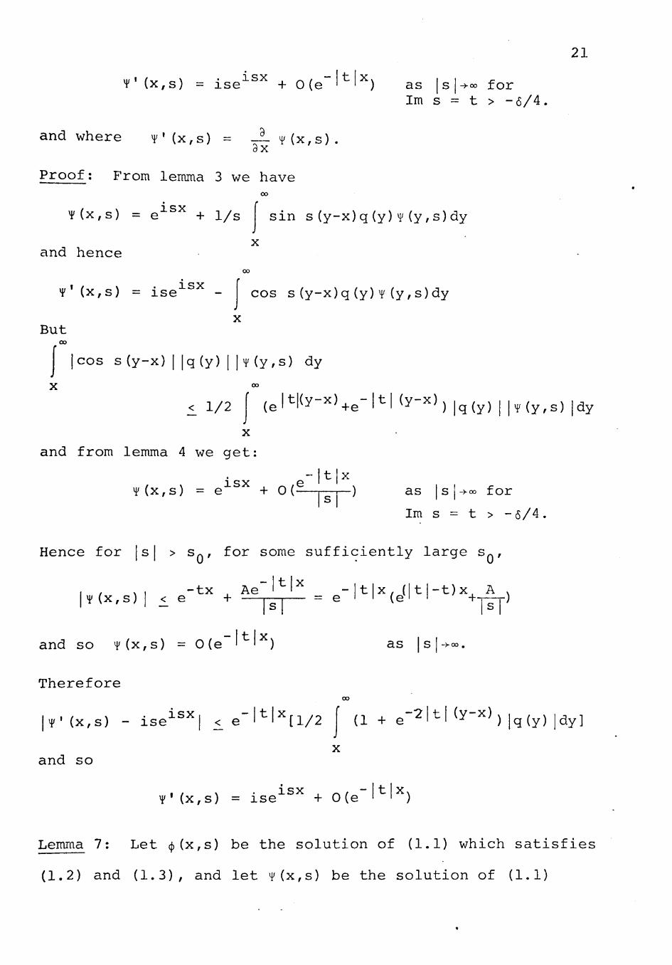
21

H*' (x,s) - isx , ^, - t X, ise + 0 (e I ' ) as I s I 00 for

Im s = t > -6/4.

and where T ' ( X , S ) = JL^^{x,s). 8x

Proof: From lemma 3 we have

H'(X,S) = e^^^

and hence

+ 1/s sin s (y-x)q (y) >!'(y,s)dy

X

1'' (X,S) = ise isx cos s (y-x)q(y)^(y,s)dy

But X

|cos s (y-x) I |q (y) I IH* (y,s) dy

< 1/2 , I t|(y-x) , - 111 (y-x) ,1 / X I I / X I -3 (e' 1'- '+e I 1' ) q(y) h'(y'S) dy

X

and from lemma 4 we get:

|t |x ^(x,s) = e + 0( 1—I—) as |s|->oo for

Im s = t > -6/4.

Hence for |s| > s^, for some sufficiently large s .,

-tx . Ae~l^l^ .-|t|x, (It |-t)x. A H* (x,s) I < e +

- t X and so 4' (x,s) = 0 (e ' ' )

= e (e ^ ^ ^

as s ->oo.

Therefore

4'' (x,s) - ise I < e I ' [1/2 (1 + e-^|tMY-^) ) |q(y) |dy]

and so

'F' (x,s) = ise + O (e ' ' )

Lemraa 7: Let (j)(x,s) be the solution of (1.1) which satisfies

(1.2) and (1.3), and let 'i'(x,s) be the solution of (1.1)

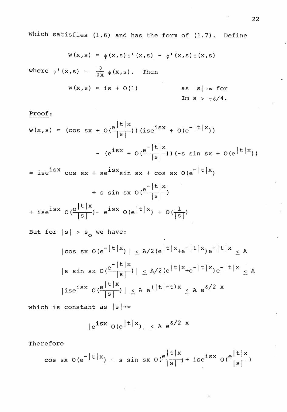
22

which satisfies (1.6) and has the form of (1.7). Define

W(X,S) = ({) (X,S) Y' (X,S) - (J)' (x,s) 4'(x,s)

where (|)'(x,s) = j^<^{x,s). Then

w(x,s) = is + 0(1) as |s|->oo for

Im s > -6/4.

Proof;

11 |x . _ I -I- I w(x,s) = (cos sx + 0(^1 1 ) ) (ise^^^ + 0 (e 1^1^))

-|t |x II - (e^^^ + 0(—-r—T-)) (-S sin sx + O(e'^l^))

ISX , ISX . , _/ - t X,

ise cos sx + se s m sx + cos sx 0(e i ' )

- t X e ' I + s sin sx 0 ( 1—I—) I s I

11 |x . II , I * l S X _ ^ , e X I S X - - / T_.X» /^/ -L X + ise 0(—I—I—)- e 0(ei I ) + 0 (-i—r) ' s s

But for |s| > s we have: I I o

t-\ / ^ X \ | •I^/'^/ i ^ X , U . X \ | C X _

COS SX 0(e ' I ) I £ A/2 (e I ' +e ' i ) e ' ' <_ A

- 111X s sin sx O(^-r-T-) I £ A/2(el^l''+e"l^l'')e'l*'l'' A

I I

• isx ^,el^l^, I , ^(|t|-t)x ^ ^ ^6/2 x ise O (—1—1—) < A e I I < A e

which is constant as s M-O°

gisx o(el*i^)| < A e«/2 x

Therefore

,t|x . |t|x cos sx 0(e'"'^'^) + s sin sx 0 ( • | )+ ise^^^ 0(^| | )

23

- e^^^ O(ei^l^) == 0(1) as |s|->co

Hence

w(x,s) = is + 0(-r-^) + 0(1)

But

0(-L_) + 0(1) = 0(1) as |s|-><

as s ->oo

and so

w(x,s) = is + 0(1) as |s|->oo

Lemma 8: Let w(x,s) be as in Lemma 7. Then

1 _ 1 1

w(x,s) ~ Ti~ " ^^TTT^ ^ 11-°° s

ProoJE: From lemma 7 we have that there exists constants

C and SQ such that

|w(x,s)-is| <_ C for |s| > s^

Then for |s| > s^:

1 1 I _ Iis-w(x,s) w(x,s) is I I isw(x,s)l — |isw(x,s)

is(is+0(l))l • ,2 ^O(l) 1 ,2 0(1) slll-

fci ' i l l I S I I

Then pick R > s^ such that 1 ^ 1 < 1/2 for |s| > R. Then

1 1 , 2C w(x,s) I¥l ^ 7-^ for |s| > R

24

and so

w(x,s) is = 7^ + 0(-i-^) as s ->oo.

This completes the proofs of the preliminary lemmas.

Chapter II

THE EXPANSION THEOREM

Theorem: Consider the system

(2.1) V" (x) + s^-q(x)) v(x) = 0

(2.2) V'(0) + Dv(0)

(2.3) lim lv(x)-e^^^| = 0 X->oo

where Im s > -6/4 and

q(y) e C[0,co) .

6/2 y e - q(y)dy < 0° for some 6 > 0 and

Let 4)(x,s) be a solution of (2.1) which satisfies (2.2)

and let ^(x,s) be a solution of (2.1) which satisfies (2.3)

and can be written in the form of (1.7) of lemma 3 in chapter

one. Let

w(x,s) = ({) (x,s) 4'' (x,s)-4)' (x,s) F (x,s)

where I _

8x Then define a Green's function for the

above system by

/

(2.4) G(x,c,s) = <

(f)(x,s)H (C.s) w(x,s)

(l)(C,s)1'(x,s)

X < c

V w(x,s) X > c

Let f(x) satisfy the following three conditions

(i) f(x) £ C^[0,-)

(ii) f(x) e L^[0,-)

(iii) f"(x) = 0(x"^) as x^'

25

26

Then f (x) can be represented as:

n m oo oo

f (x) = 2 I Res (s, ) + I Res {x, ) - X • k = l k j^^j^ ' k 7T1

where {s, : k=l,...,n} are the poles of

0

G(x,C/S)f ((;)d(c)sds

G(x,c,s)f (c)dc

0

in the upper half of the s-plane and {x, : k=l,...,m} are oo

the poles of s G (x,c,s)f ( )dc which can be on the real

0 axis, where it is assumed that all poles on the real axis

are simple poles.

Proof: Let (^(x,s), 'i'(x,s) and V7(x,s) be as indicated in

the theorem. Then w(x,s) is dependent of x [2]. Since

both ^{x,s) and r(x,s) are analytic functions of s for

Im s > -5/4, w(x,s) is an analytic function of s for Im s >

-6/4, and so the Green's function, which is given by (2.4)

is meromorphic function of s for Im s > -6/4, with poles

possible at the zeros of w(x,s).

Let the contour r , in the s-plane, be given by

Figure 1

27

where the semicircle is denoted by C^ and r ^ = C„{x: -R<x<R}

K R R — — From Lemma 8 we have that

w(x,s) is • + 0 ( — ^ ) as I s |-)oo for

Im s > -6/4

and so s G (x, , s) f ((;) d^ cannot have any poles outside of

0

some r p for R sufficiently large. Also, the poles of

G(x,5,s)f(^)d^ are isolated, and so there can only be a

finite number of poles in the upper half plane and on the

real axis.

In order to obtain the expansion formula associated

with (2.1)-(2.3) we must evaluate

I-, = lim —r-0 ^ TTl

G(x, ,s) f (^)d^)sds

r ' 0

by contour integration and by residues

Fix R such that:

(i) R ^ Spj, where s^ is such that all 0-inequalities

hold for IsI > SQ.

(ii) no poles of s G(x,^,s)f(^)d^ lie outside of r R

0

Also assume for the present discussion that no poles lie on

the real axis. Then

28

Tvi G ( x , c , s ) f ( ; ) d c ) s d s = TTl

^S'F ( x , s ) w ( x , s )

(})(C , s ) f ( ( ; ) d ( ; ) d s

^R ° 0 R

TTl

/S^ (x^.s) w ( x , s ) H'(c , s ) f ( c ) d c ) d ^ = X ^

T T l [e^(x,s)+e2 ^^'^^ ^^^

R

+

X

TTl

'R R

[e-| (x,s)+e2 ^^'^^ ^^^ R

where 9-, (x,s) and 0 2(x,s) are given by

sy(x,s) X

e. (x,s) = " p^" 1 w(x,s)

((> (C/S)f (c)d(;

0

02 (x,s) S4) (x,s) w(x,s) y(C/S)f(c)dc

Substituting the approximations for (^(x,s), 4'(x,s) and

(x,s) given in the previous chapter, e,(x,s) and ep(x,s) w

become:

-|t|x . , e-^(x,s) = [-ie ^ '-l 0(^ u I ) + se'- '' ^ 7 ^ ^

+ sO(--|t|x rX

'• ^)]

|t| (cos s c + 0 {%—r))f (c)dc

But the integration is over r p and for s on r , Im s = R R

t > 0 and hence, Itl = t and le I = ^ < 1 for all

X ^ 0. 0,(x,s) then becomes

29

ISX -tx -tx -Itlx

e^(x,s) - [-ie— + 0(^. I ) + O(V-T-) + 0(" o )]

0 |t|c

(cos sc + 0(^—T-))f ( )dc

= [-ie - + 0(V^)] 0 |t| c (cos s c+ 0(^——))f ( )dc

= -le ISX

0 ISX

COS scf(c)dc -ie-^"^ 0 (", | )f(c)dc tk

X X

-tx 0

cos s^ f(^)d^

X

+ 0( I I )

-tx r^ tC, 0(j^)f (C)dc = 1^ + 12 + 13 + 1

X

Likewise

T tx 1 e

0p(x,s) = [-i cos sx + s cos sx 0( p) + sO (-1—p)

tx

I o I (e - ^ + 0(?—r))f(c) d^

0

tx tx tx [-i COS sx + 0(?—^) + 0(^ 5-) + 0(?-|-)]

(e -tc

''^^ + 0(^1—r))f {c)dc

X

tx [-i cos sx + 0 ( —r) ] (e

-ti; "" ^ + 0(?-r-))f (c)dc

X

= -1 cos sx 1 ^ f(^)d^ -i cos sx

X X

30

e^^ tx e- '' f(c)dc + O ( ^ ) ,e-^?

o(^n-^)f U)dc X X

= I 5 + Ig + I , + I g .

It will now be shown that: X

( 2 . 5 ) l i m R->oo

( I 2 + 1 3 + 1 4 + 1 ^ + 1 ^ + I g ) d x = 0

0

and

X

( 2 . 6 ) l i m R->oo TTl

( I ^ + l 5 ) d s = f ( x )

0

I , = - l e

We consider (2.6) first: X

isx cos sC f(C)dC and integrating twice

0

by p a r t s I , b e c o m e s :

. i s x r S i n s x ^ , , . c o s s x ^ , , , f (0) 1^ = - l e [— f (x) + 2 — f (^) ~ — ^ ~ ^

X

0 s

B u t

X

_ ^ ^ i s X j C O S S X f , , ^ j _ f M O l

1 {?

s

- t x

c o s _ s ^ f " ( c ) d c ]

0

2 ^ 2 [e ^^ + e ^ ^ ] I f (x) I + e ^ ^ I f ' (0)

-tx X

(e ^^+e^^) If" (c) Idc)

0

Let K^ = max {f' (x) , ^—^ , f' (c) }. Then the above 0<c<x ^

becomes:

31

< _ 1 _ . K„ {e-2tx + 1 + e-^^ + e-^^ ^(e^^-e-^^) l""} ^ 0

X

1 - ^ K {3 + 1 - e ^ }

Isr t

which implies T . isx sin sx ^, , . , 1 x 1^ = -ise — f(x) + 0( 2^

ise Ic = -1 COS sx e ^f(c)dc and integrating twice by

X

parts, Ic- becomes:

ISX ISX

Ic = -i cos sx [ : f (x) - 7^ f' (x) -5 IS 2

f ISC e

k s f"(c)dU

But

ISX -i cos sx [ ^ f ' (x)

00

r is e f"(Odc]

tx. -tx -tx s +e 6 I £ I / \ I .

1 2 7-72 1 <' ' I + s

-t f"(0 Idc

^ s X

{ f (x) + f"(c) Id?}

But f" ( C) = 0 ( y) implies that there exists an x- such Id "

32

that for c > XQ |f"(5)| <_ M • 1/^ for some constant M. Then

X 0

f"(c) |dc <. |f"(c) |dc + M . 2 ^? X.

. 0 f" (c) \^K + V x 0

X

and hence

ISX -i cos sx [- ^ f' (x) -

00 , r isr e ^

2 f"(ddc]

X X 0

{ If (x) I + f"(c) I dc + M/XQ}

X

and so

ISX ^5 = COS sx f (x) + 0( r) as |s|->oo

Then (2.6) becomes

l im R->oo

TTl ( I ^ + l 5 ) d s

R

= l im R->oo TTl

I S X , , . I S X s m S X , e , { ( - l e + cos sx)

' R

f (x) + 0(—i-^) }ds

= l i m R

TTl f(iiiLL + o ( - ^ ) } d s = l im • 1

->oo R ->oo TTl

'R 0

( • ( l i ^ + o ( - ^ ) ) i R e ^ ^ d 0 Re^^ R^

l i m — R->oo

TT ,TT

1 6 {f (x) + 0 ( 1 / R ) ) e "}d0

0

= f ( x ) + l im R->oo >

0 (1 /R)e^^d0

0

But l i m R->oo

^ T T

0 ( 1 / R ) e ^ ^ d 0 ,TT

<_ l i m R->oo

K/R d0 = l im KTF/R = 0 R^oo

0 0

33

and hence

lim R->oo

Now consider (2.5)

TTl (IT + Ir:)ds = f (x) .

1 D

'R

X

. ISX

1-2.= -le 0 ( ^ ) f (C)dc

0 Let s = Re^^ , ds = iRe^^d0. Then

l2ds = . iRe X -le

6 0

0(^i|ill^i)f(,)d, iRe^^de

R TT X

iRx cos 0 - Rx sin 0 Rg-*- R sin 6

0(^ 5 )f (C)dcd0 K.

0 0

and for R > s 0

TT X

l2ds| <. -Rx sin 0 „ e • M

R sin 0c|f (c) |dcd0

0

1 ^1

R TT X - A

-Rx sin 0 r e I

0 X

0 0

R sin ec d^ ^ f eR sin 0c ^^^

x-A

where M is the 0-constant and M, = M • max |f(c) 0<c<x

< 2M. -R sin 0^^R(x-A)sin 0 (x_^) + g^^ ^^^ ® • A]d0

0 TT

= 2M. ^^-RA sin 0(^_^) ^ ^]de

0 2M, TTA

Let e > 0 and pick A such that — 2 — < e/2. With the

R A 2 ^ T . ^ - R A s m 0 - 0 0 < 0 < TT/2 t h e

i n e q u a l i t y e ^ e T T U ^ U ^ T T / ^ unt;

a b o v e b e c o m e s : < M . | f ( x ) | _ i ^ (1 + e"^^"") 1 2 M | f ( x ) | • 1 s I

34 for I s

and so

> s 0

0 { ^ ) iiil-^ f(x) = 0 ( - ^ )

Also

0(5;5!)|[SilL4if'(x) - f ' Q ' X

COS S f"(c)dc]

tx tx -tx

< 0(V^t^|f'(-)| ^~2

0

f (x) I + f (0)

X

+ (e '+e ^'') lf"(^) Id^]

0

Let K - max { |f' ( ) | , |f (o) | , |f" ic,) \ } and then for 0< c<x

s > s^ the above becomes

X -- M n , -tx, -tx, -tx, -tx

< K • T" [1 + e +e +e +e

2tx . K • ^ [ 3 . ^ ^

I" (e^^+e ^^)d^]

0

and so

13 = 0 (—^) + 0 (-^) as s ->oo

-tx

4 = ° ( ^ : X tc 0 ( ^ ) f (C)dc

0

and for |s| > s^, |I.| becomes

tx . t, I . < M =-r— 4 I — s

f (d I C < K-M -tx . 1, tx ,

rT2^ t^^ -1 0

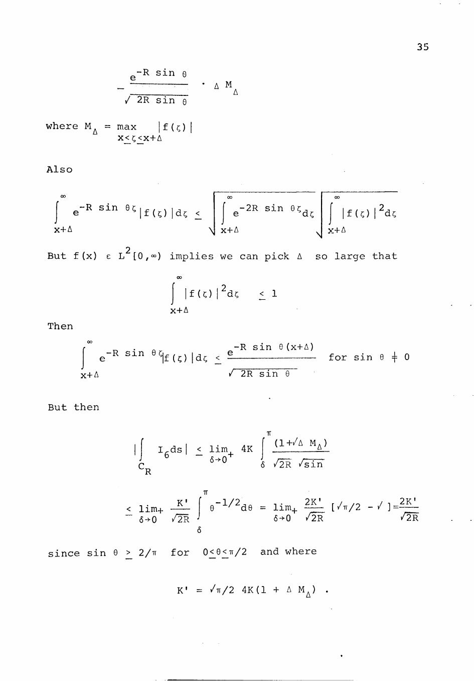
35

-R s i n 0

/ 2R s i n 0

• A M A

w h e r e M. = max | A I

x<c<x+A

f (C)

A l s o

-R s i n 0C 14= / \ 1 J e ^ f ( c ) dc <

X + A

-2R s i n 0C-, e ^dc

NJ X+A N

f ( C ) I d c

X + A

B u t f (x) e L [0,°°) i m p l i e s we c a n p i c k A s o l a r g e t h a t

| f ( O I dc < 1

x+A

Then

^ - R s i n e c | f ( ^ ) . ^ ^ , e -R s i n 0(x+A)

x+A

f o r s i n G =f 0

/ 2R s i n 6

B u t t h e n

TT

I , d s | < l i m ^ 4K ^ ~ 6- 0"^

f (1+/A M J A

R 6 /2R / s i n '

TT

< l im+ K' f 0 - V 2 ^ 0

6-^0 /2R = l i m . 2K V I

[ / T T / 2 - / ] = 2K

6-^0 /2R 2R

l i n c e s i n 0 > 2/TT f o r O < 0 < T T / 2 and w h e r e

K' = / T T / 2 4K(1 + A M.) .

Therefore

lim R->co

Igds I £ l im ^ ^ = 0 R->oo / 2 R

R

X

and integrating twice by parts I^ becomes

tx ISX ISX 00

r ISX

e I7 = O ( ^ ) [- ^ - ^ f (X) - £j^f(x) - £-^f"(,)d5] i S

X

But proceeding as with I , we have

tx isx 0(?^)[- ^-2-f(x)

00

r ISX

e 2-f' ( d d ^ = 0 ( - ^ )

and

36

tx isx . |f(x)

where K is the 0-constant. Hence

I7 = 0( o) as s ->oo

and so

TT

lim R->oo

tx

^8 = 0 <fiT)

I^ds = lim — K-)-oo

0

-t,

d0 = 0

tx 0 ( )f(c)dc = O(^) J

X

0(e •^^)f(^)d^

X

and Ij ds can be evaluated in the same manner as was

R

37

Igds. Hence

'R lim I R->oo J

Igds = 0 .

'R Combining these results, (2.5) follows, that is.

l i m R->-00 •'

d o + i_ + i ^ + I 6 + 1 ^ + l 3 ) d s = 0

'R

Now, c o m b i n i n g ( 2 . 5 ) and ( 2 . 6 ) we o b t a i n

l i m R->00

TTl [ 0 j ( x , s ) + 0 2 ( x , s ) ] d s = f ( x ) .

'R I Q t h e n b e c o m e s

0 = f(- ' + ;T TT-

[0j^ ( x , s ) + 02 ( x , s ) ] d s

and then evaluating I^ by the theory of residues v/e have 0

f ( x ) = 2 \ R e s ( s , ) - X K T y l

00 00

{ G ( x , c , s ) f ( c ) d c } s d s

0

w h e r e ( s , : k = l , . . . , n } a r e t h e p o l e s of s G ( x , ; , s ) f ( ^ ) d ^ J 0

in the upper half of the s-plane. As was noted earlier,

the sum of the residues is a finite sum.

We assumed, in the previous discussion, that

G(x,c/S)f(^)dc had no poles on the real axis. Now

suppose that s G(x,?,s)f(c)d^ has some real poles. Again

we know that it can have only a finite number of such poles.

38

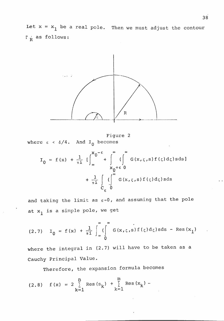
Let X - x^ be a real pole. Then we must adjust the contour

r • as follows:

Figure 2 where e < 6/4. And I^ becomes

I = f (x) + -j-0 T T l

^ 0 - ' 00 00

+ (

X Q + S O

G ( x , c , s ) f ( ^ ) d ^ ) s d s ]

+ TTl (

C 0

G (x , <;/S)f ( c ) d ( ; ) s d s

and taking the limit as e->0, and assuming that the pole

at X, is a simple pole, we get

(2.7) IQ = f(x) + ^

CO oo

r (

00

0

G(x,^,s)f(^)d^)sds - Res(x^)

where the integral in (2.7) will have to be taken as a

Cauchy Principal Value.

Therefore, the expansion formula becomes

n m (2.8) f(x) = 2 I Res(Sj^) + I Res(Xj^)

k=l k=l

39

00 00

TTI ( G(x,c,s)f(c)dc)sds

where (Sj^: k=l,...,n} are the poles in the upper half o

the s-plane and {x^: k=l,...,m} are the real poles of

G(x,c,s)f (c)dc.

Chapter III

TWO EXAMPLES

We conclude this paper with two examples. For the

first example we consider one of the examples in Cohen's

dissertation. For the second example we let q(x) = -^^e~^^^

and show that for B sufficiently small, and positive, the

conditions of the expansion theorem are satisfied.

Example 1: Consider the system

(3.1) v" (x) + s^v(x) = 0 0 < ^ x < a > , i m s > _ 0

(3.2) V'(0) + D v(0) = 0 D e c

(3.3) lim |v' (x) -isv(x)| = 0 X->oo

In order for this system to satisfy the conditions of the

expansion theorem, it is necessary to show that the solution

i|;(x,s), which is given by lemma 3 of chapter one, also sat­

isfies (3.3). But this is obviously true since i|;(x,s) = e

and e satisfies (3.3).

The solution, i>{x,s), of (3.1) which satisfies (3.2)

and which is given by lemma one of chapter one, is:

<\> (x,s) = cos sx - D/s sin sx

w(x,s) then becomes:

w(x,s) = (cos sx - D/s sin sx)ise

+ (s sin sx + D cos sx)e

40

41

= D + is

The Green's function is given by:

r

G(x, ,s) =<

(cos sx - D/s sin sx)e^^^

D + is

(cos s^ - D/s sin sc)e^^^

D + is

X < ;

X < 5

The only pole of s G (x,^,s)f(^)d^ is located at s = iD

and it is a simple pole. The expansion formula can take

three different forms depending on whether Re(D)>0, Re(D)=0

or Re(D)<0.

Define

r 2 Re(D) > 0

0 (D) ={ 1 Re(D) = 0

0 Re(D) < 0

and the expansion formula becomes

00 ,

ISX |.X

6 f(x) = 0(D) Res(iD) - X\ {?f—-

TTI is+D (cos SC - D/s sin S(;)f(i;)d(;

. s (cos sx - D/s sin sx) f isr ^, .^ , ^ + '- e '' f (c)d(;}ds

X IS + D

Then, breaking the integral with respect to s into an

integral f rom - oo to 0 and an integral from 0 to oo, and mak­

ing the change of variables s = -a in the first integral

and s = a in the second integral, we get

42

f ( x ) = 0(D) R e s ( i D ) - i J"^-''i§+^; / ^ ( c o s ac - D/t s i n a c ) f ( c ) d c - l a X

0 --*+^ 0

a ( c o s ax - D/a s i n ax ) /•«> -ioz; ^ -} e ^ f ( c ) d c } d a

iD + a X

l a x 2_ f°°r e rX 7 i ^ -in-r^ i ( c o s ac - D/a s i n a c ) f ( c ) d c TT Q l u a Q

+ o^(cos a x - D/a s i n ax) J°° e^"^ f (C ) dc) d a iD - a X

and combining terms we have

f(x) = 0(D) Res(iD) + 2 J- a^ (cos aX - D/a sin ax) "" 0 D^ + a

/ ~ ( c o s a C - D/a s i n a c) f ('^)d'^do' 0

w h e r e

R e s ( i D ) = R e s i d u e o f s/*° G (x , c /S) f (c) dc a t s = iD 0

0

This result agrees with Cohen's result.

Example 2: Consider the system

(3.4) v" (x) + (s^ + B^e"^'^)v(x) = 0 0 ^ x < «>

(3.5) v' (0) + D v(0) = 0

I / \ isxi « (3.6) lim I v(x) -e 1 = 0

X->oo

43

where a, 6 e R and a > 0 , Ims> - ^ r. T -; i yj, ±m s > - - —- and D IS a complex

constant.

Note t h a t q (x ) = g V ^ ^ i s c o n t i n u o u s on [0 , ^ ) and

f o r 6 = 1 /a ,

r e ^ / 2 X g ^ ^ ^ ^ ^ ^ 32^00 ^ x ( l / 2 a - 1/a) ^^ _

0 0

In order to find solutions for the above system, we make

the change of variables:

il = s and t = -x/2a

and get:

(3 .7 ) v " ( - x / 2 a ) + (4a^3^e^^ - 4 a ^ l ^ ) v ( - x / 2 a ) = 0

which h a s s o l u t i o n s of t h e form:

V, ( x , s ) = J ^. (2a6e~^/^ ' ' ) 1 ' . - 2 i a s

v ^ ( x , s ) = Y o- (2a6e~^/^° '^ 2 - 2 la s

The solution which satisfies (4.2) and which is given

by lemma one of chapter one is:

(3.8) ^(x,s) = a(s)v^(x,s) - b(s)v2(x,s) c(s)

where

a(s) = d/dx V2(0,s) + D V2(0,s)

b(s) = d/dx v^(0,s) + D v^(0,s)

44

c(s) = v^(0,s) d/dx V2(0,s) - V2(0,s) d/dx v^(0,s)

In order to find a solution which satisfies (4.3) and

has the form of lemma three of chapter one, we consider

the function

h(x,s) = k(s) v-j (x,s) Im s > 0

and solve the following equation for k(s):

(3.9) k(s) V (x,s) = e^^^ + ^/~sin s (y-x)q (y) k (s) VT(y,s)dy. ^x ^

Solving, we find that:

k(s) = ^^-^^^^-T^^ (a6)-2^^^

Then, using two equalities from [7], page 484, numbers

11.3.20 and 11.3.21, it is easily shown that for the above

value of k (s) , k(s) v, (x,s)- satisfies (3.9) for all s such

that Im s > - 6/4 and hence

(3.10) ^p (x,s) = k(s) Vj^(x,s)

is a solution of (3.4) v/hich satisf-ies (3.6) and has the

form of lemma three, chapter one.

On computing w(x,s) we get:

(3.11) w(x,s) = k(s)[d/dx v^(0,s) + D v^(0,s)]

and in order to be able to use the expansion theorem we

must show that the real zeros, with respect to s, of w(x,s)=0

if any such zeros exists, are simple zeros.

45

Let s be real and consider

(3.12) k(s) v^(x,s) = e

1 s

ISX

sin s (y-x) 3 e ^ ' k(s) v^(y,s)dy

X

Substituting (3.12) into (3.11), the equation w(x,s) = 0

is equivalent to:

(3.13) is + D + (cos sy - D/s sin sy)

0

X B^e / ^ k(s) v^(y,s)dy = 0

ReD = Re(-

But if s is a real zero of (3.13) then we must have

00

(cos sy - D/s sin sy) ^^e'^^"" k(s) v^(y,s)dy)

0

and

s + Im D = Im(-

0

X

(cos sy - 'D/s sin sy)

B^e-y/^' k(s) v^(y,s)dy).

By using (3.10) and a modification of Gronwalls inequality

[8], it can be shown that

k(s) v^(x,s) I f_ e

00 •-"

and so

k(s) v-j (x,s) I 1 e 2o2

a 6

But then

46

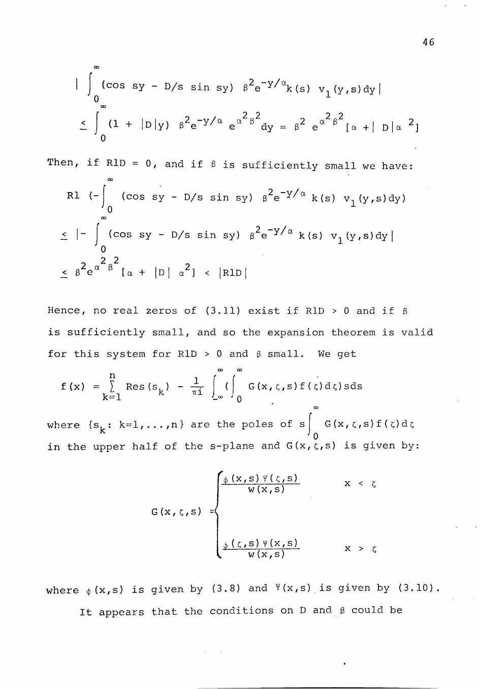
I (cos sy - D/s sin sy) 3 e ^/\(s) v-,(y,s)dy 0 1

(1 + |D|y) 3 V ^ / ^ e^'^'dy = 3 e"'^'[a +| D|a ^j 0

Then, if RID = 0, and if 3 is sufficiently small we have:

Rl (-

'o (cos sy - D/s sin sy) 3 e ^^"^ k(s) v^(y,s)dy)

(cos sy - D/s sin sy) 3^e~^^°' k(s) Vj^(y,s)dy 0 2 2

< 3 e°' [a + JDJ a^] < |R1D

Hence, no real zeros of (3.11) exist if RID > 0 and if 3

is sufficiently small, and so the expansion theorem is valid

for this system for RID > 0 and 3 small. We get

n 00 00

f (X) = 5: Res(s ) - X k=l ^ ""

( G (x, C/S) f ( c)d(;)sds 0

where (s, : k=l,...,n} are the poles of s G(x, c,s)f (c)dc 0

in the upper half of the s-plane and G(x,c,s) is given by:

%(x,s)y(c.s) w(x,s)

X < C

G(x,c,s) <

j) (c.s) y(x,s) w(x,s) X > C

where <i^{x,s) is given by (3.8) and H'(x,s) is given by (3.10)

It appears that the conditions on D and 3 could be

47

relaxed, but it would again be necessary to prove that the

real zeros of w(x,s), if any exist, are simple zeros.

LIST OF REFERENCES

1. Buck, R. C. Advanced Calculus, 2nd edition. New York: McGraw-Hill Book Co., 1965. Pp. xii + 527.

2. Coddington, E. A., and Levinson, N. Theory of Ordinary Differential Equations. New York: McGraw Hill Book Co., 1955. Pp. xii + 429.

3. Cohen, D. S. Separation of Variables and Alternate Representations for Non-Self-Adjoint Boundary Value Problems. Ph.D. Dissertation, New York University, 1962. Pp. 79.

4. Dettman, John W. Applied Complex Variables. New York: The Macmillan Co., 1965. Pp. ix + 481

5. Friedman, B. Principles and Techniques of Applied Mathematics. New York: John Wiley and Sons, Inc., 1956. Pp. ix + 315.

6. Gray, A., and Mathews, G. B. Bessel Functions and Their Applications to Physics. London: The Macmillan Co., 1931. Pp. xiv + 327.

7. Abramowitz, M. and Stegun, I. A., Ed. Handbook of Mathematical Functions. Washington: U.S. Government Printing Office, 1964. . Pp. xiv + 1046.

8. Hartman, P. Ordinary Differential Equations. New York: John Wiley and Sons, Inc., 1964. Pp. xiv + 612.

9. Titchmarsh, E. C. Eigenfunction Expansions Associated with Second Order Differential Equations. Oxford: The Clarendon Press, I, 1946. Pp. 186.

48