An Empirical Model for Vane-Type Vortex Generators in a ... · American Institute of Aeronautics...

American Institute of Aeronautics and Astronautics

1

An Empirical Model for Vane-Type Vortex Generators in a Navier-Stokes Code

Julianne C. Dudek* National Aeronautics and Space Administration

Glenn Research Center Cleveland, Ohio 44135

An empirical model which simulates the effects of vane-type vortex generators in ducts was incorporated into the Wind-US Navier-Stokes computational fluid dynamics code. The model enables the effects of the vortex generators to be simulated without defining the details of the geometry within the grid, and makes it practical for researchers to evaluate multiple combinations of vortex generator arrangements. The model determines the strength of each vortex based on the generator geometry and the local flow conditions. Validation results are presented for flow in a straight pipe with a counter-rotating vortex generator arrangement, and the results are compared with experimental data and computational simulations using a gridded vane generator. Results are also presented for vortex generator arrays in two S-duct diffusers, along with accompanying experimental data. The effects of grid resolution and turbulence model are also examined.

Nomenclature c = vortex generator chord length Et = total energy h = vortex generator height I, J, K = directions on the computational mesh i, j ,k = indices indicating the ξ,η,ζ directions on the computational mesh l = vortex generator index Pt = total pressure u = x-direction component of velocity un = normal component of velocity up = parallel component of velocity u_pj = J-direction component of the parallel velocity u_pk = K-direction component of the parallel velocity v = y-direction component of velocity w = z-direction component of velocity R = distance from vortex generator tip Tt = total temperature Vmax = core velocity x, y, z = Cartesian coordinates y+ = nondimensionalized y-coordinate α = vortex generator angle of incidence δ = boundary layer thickness Γ = circulation ρ = density ωmax = peak vorticity ξ,η,ζ = computational coordinates

A. Subscripts i,j,k = indices indicating the ξ,η,ζ directions on the computational mesh l = vortex generator index * Aerospace Engineer, Inlet Branch, 21000 Brookpark Road and AIAA Senior Member.


2

I. Introduction he subsonic diffusers of modern aircraft engine inlets encounter very challenging flows often characterized by strong adverse pressure gradients, boundary layer separation, and strong secondary flows. These flows may

result from various factors including large amounts of diffusion taking place over short lengths; flow path turning; ingestion of boundary layers; upstream vortices and wake disturbances; and upstream shock-wave boundary layer interactions. Surface-mounted vane-type vortex generators (VGs) are often used to counteract these effects using one of the two following strategies. The first strategy uses vortices to mix the low-momentum boundary layer flow with higher momentum core flow to help reduce or eliminate boundary layer separation. In the second strategy, the vortices are used to favorably redirect secondary flows. In both situations, the goal is to improve the performance at the engine face by increasing engine face total pressure recovery and decreasing engine face distortion.

Computational fluid dynamics (CFD) is used to simulate inlet flows and predict inlet performance, and together with experiments, is also useful in designing new inlets. Since VGs have the potential to greatly improve the performance of an inlet, it is highly desirable to include the effects of vortex generators in these simulations. However inlet geometries typically include multiple VGs, and in studies where multiple VG arrays must be analyzed and/or VG arrays must be designed, it is neither practical nor desirable to generate the computational grids required for each VG in terms of both the time and effort spent on grid generation, as well as the added computational time required to compute the additional grid points necessary to resolve the VG geometry and surrounding flow details. Therefore, it is highly desirable to be able to model the effects of the VGs without including their geometry in the computational mesh.

With this in mind, the Wendt empirical VG model1,2,3 was developed at NASA Glenn and implemented into the publicly available Wind-US Navier-Stokes code.4,5 This VG model simulates vortices shed from one or more wall-mounted vane-type generators in a flowfield. It was developed primarily for inlet flows and was derived using classical fluid mechanics correlated with experimental data. The implementation of this model into the Wind-US code takes the form of a boundary condition specified at a coupled zonal interface. The vortices produced by a single vortex generator or an array of vortex generators are simulated by a step change in secondary velocities across a zonal interface. The model determines the strength of each vortex based on the user input vortex generator chord length, height and angle of incidence with the primary flow, as well as the local velocity and boundary layer thickness.

In the present work, the Wendt vane-type VG model, its implementation into the Wind-US code, and usage guidelines are described. Results of a validation study for flow in a straight pipe with a counter-rotating vortex generator array are presented, and the model simulations are compared with simulations using gridded VGs and with experimental data. Validation results are also presented for flow in a transitioning S-duct diffuser and a circular S-duct diffuser comparing both with experimental data. The effects of turbulence model and grid resolution are examined.

II. The Wind-US CFD Code The Wind-US CFD code may be used to solve the Euler or Navier-Stokes equations of fluid mechanics, along

with supporting equation sets governing turbulent and chemically reacting flows.4,5 Previous versions of the Wind code allowed for only structured grids, however, the recently released Wind-US (“US” stands for “unstructured-structured”) code, also has unstructured and hybrid grid capability, although all cases described in this paper use only structured grids, and the vortex generator model is currently valid only for structured grids. The Wind-US code is the production solver of the NPARC Alliance, which is a partnership between NASA Glenn Research Center (GRC), the USAF Arnold Engineering Development Center (AEDC), and the Boeing Company. The mission of the Alliance is to develop, validate and support an integrated, general purpose, computational flow simulator for the U.S. aerospace community; the work described in this paper contributes to these efforts. The code itself uses a finite-volume formulation and allows the user to select from several schemes to compute both the right-hand-side inviscid terms, as well as the left-hand-side viscous terms.

III. The Vortex Generator Model

A. Formulation The vortex generator model of Wendt1,2,3 is used to simulate the vortices shed from one or more wall-mounted

vane-type generators in a flowfield. This comprehensive model was developed with inlets in mind, and is based on derivations using inviscid theory and conservation of momentum correlated with an extensive collection of data from experiments performed with vortex generators having flat plate and symmetric NACA 0012 profiles and

T


3

mounted in a cylindrical duct. The strength and concentration of each vortex is a function of the VG chord length, height, angle of incidence and the local freestream velocity and boundary layer thickness.

The model uses the Eqs. (1) – (4) to compute the secondary velocities of the vortices at a given zonal interface boundary. The vortices are first computed using boundary variables (ρun, up, Pt, Tt), then converted to conservation variables (ρ, ρu, ρv, ρw, Et) before being passed from the subroutine. The current implementation of this model into Wind-US assumes that the primary flow direction is the ξ-direction, and the secondary flow directions are the η- and ζ-directions. On an i = constant boundary, the secondary velocities are given by u_pjj,k,l and u_pkj,k,l. (See Eqs. 1 and 2.) These are the j- and k-components of the parallel velocity up, at (xj,k, yj,k, zj,k), resulting from a vortex shed from generator l with it’s trailing edge tip located at (xl, yl, zl).

( )

2,

,,,, 2

_kj

kjlkjllkj R

Fzzpju

π−Γ

= (1)

( )

2,

,,,, 2

_kj

kjlkjllkj R

Fyypku

π−Γ

−= (2)

Where, ( ) ( ) ( )2222

, zyxR kj ∆+∆+∆= And

lkj xxx −=∆ ,

lkj yyy −=∆ ,

lkj zzz −=∆ , Also,

⎟⎟

⎠

⎞

⎜⎜

⎝

⎛

Γ−

−=l

kjlkj

RF

2,

max

, exp1πω

In the above equations, Γl represents the circulation or strength of vortex l, and max

lω represents the peak vorticity, located at the center of the vortex, which is also indicative of the vortex concentration. For an array of vortex generators, i.e. when there are multiple vortex generators mounted on the viscous walls of the zonal boundary interface, the secondary velocity fields produced by the presence of the individual generators are superposed as shown below, where m is the number of generators.

∑=

=m

llkjkj pjupju

1,,, __

∑=

=m

llkjkj pkupku

1,,, __

Note that the Wendt model also adds image vortices which account for the influence of the viscous wall

boundary on the shed vortex.3 Image vortices are currently omitted from Wind-US implementation of the vortex generator model, however the viscous wall effects that are inherently present as the vortices are convected downstream may be sufficient to make up for this omission.


4

The following formula approximates the circulation of the shed tip vortex, and is based on Prandtl’s inviscid airfoil theory.6

ARk

hkcVk

l2

3max1

1

tanh

+

⎥⎦

⎤⎢⎣

⎡⎟⎠⎞

⎜⎝⎛

=δ

αΓ (3)

Where the aspect ratio, AR, is

chAR

π8=

And h is the height of the generator, c is the chord length, α is the angle of incidence the generator makes with

the primary flow, Vmax is the core velocity and k1 through k3 are constants derived through least squares regression with experimental data and have the following values: k1 = 1.61, k2 = 0.48, k3 = 1.41.

The peak vorticity maxlω is derived from equating the rate of angular momentum production to the sum of the

moments at the VG tip. The resulting formula is given below:

( )2

max2223

23max

2

1

Vhcl

lαπ

βω −Γ= (4)

Where

( )22/12 121

−−ψ=β

e

And ψ = 0.29 as determined by a least squares regression from experimental data.

Note that this vortex generator model was designed to be applied at a streamwise location one chord length downstream from the trailing edge of the generators. This is the station where the experimental data was measured because previous work indicates that at this location, the vortices are fully formed such that the circulation and peak vorticity are at their maximum values.

B. Implementation and Usage The vortex generator model was incorporated into the Wind-US CFD code in a manner similar to existing

actuator disk/screen boundary conditions. It acts as a boundary condition which is specified at coupled zonal interfaces. This vortex generator boundary condition is invoked by specifying the VORTEX keyword block in the standard Wind-US input data file.5 It produces a step change in secondary velocities, simulating the vortices shed from the generator or an array of generators, across the boundary. As mentioned above, the vortex generator model determines the strength of each vortex based on the user-specified generator chord length, height and angle of incidence with the incoming flow, along with the local core velocity and boundary layer thickness. Figure 1 illustrates these parameters. To derive the model, experimental data with the following parametric ranges were used: 0.13 < h/c < 2.62, 0.12 < h/δ < 2.60, and the Mach number between 0.20 and 0.60. A maximum of 10 vortex generator arrays is allowed and each array may have a maximum of 20 generators. The code places each vortex center at the grid point closest to the VG location determined by the user-specified generator location on the wall boundary, and the generator height. The model is only applicable to generators placed on viscous wall boundaries. Examples using the VORTEX keyword block are given with each validation case presented in this paper.

Note that, as previously mentioned, the vortex generator model is derived from experimental data taken at axial stations which were one chord length downstream of the trailing edge of the generators, and therefore the secondary velocities produced by the model simulate vortices at this station, rather than at the generator trailing edges. For most accurate results, the zonal interface boundary where the vortex generator boundary condition is applied should be at this one chord length station.


5

The secondary velocities which represent the vortices are computed from Eqs. (1) and (2) above. To avoid the singularity at the vortex core, where 2

,kjR approaches zero, 2,kjR is set to 0.001hl

2 if the actual computed value is less than 0.001hl

2. The static flow properties must also be updated to correspond to the change in the secondary velocities. Since the vortex generators will generally be small compared to the cross section of the flowfield in which they are placed, and the secondary flows produced by these generators will generally be weak compared to the kinetic energy of the primary flow, it is reasonable to treat the vortices as free vortices (irrotational) which have isentropic turning throughout. Conservation of normal momentum (ρun) is assumed at each point on the zonal interface boundary and the new static conditions (pressure, temperature, and density) are computed from the compressible Bernoulli equations.7

IV. Pipe Flow Analysis The initial validation case investigated with the proposed VG model is a Mach 0.25 flow through a constant-

area straight pipe with counter-rotating pairs of vane-type VGs spanning the circumference. In addition to simulations using the VG model, simulations were also done with the generator gridded as a flat-plate vane. Approximating the VG geometry as a flat plate saves time and labor compared to gridding up the airfoil shape of the VG. Previous studies in subsonic ducts have shown the downstream flows of the gridded flat plate vane and a gridded airfoil to be very similar.8 Results are compared with the experimental data of Wendt et al.3

A. Experimental Configuration The duct tested in Ref. 3 was a constant area pipe 237.5 cm in length. The inner diameter of the pipe, d, was

20.4 cm. The core Mach number was 0.25. The VGs were mounted in the duct at an axial station 93 cm from the entrance, where the core velocity was 85 m/s and the boundary layer thickness was approximately δ/d of 0.04. The pipe had twelve VGs, each with a NACA0012 profile, a chord length c of 4.06 cm, a height h of 1.02 cm, and an angle of incidence α of +16°. They were equally spaced around the duct circumference in a counter-rotating arrangement. The circumferential spacing between the mid-chord positions of the VGs was 30°. A schematic of the duct is shown in Fig. 2.

B. Computational Grid Due to the symmetry of this geometry, only a 30° section of pipe was modeled with the computational grid. One

VG was placed within this sector and symmetry boundaries were used to simulate the adjacent VGs. For the cases in which the VG geometry was included in the grid, its geometry was approximated as a flat plate, as mentioned above, since this saves time and labor as opposed to gridding up the airfoil shape of the VG. The length of pipe included in the grid was somewhat longer than the pipe in the experiment to allow the VG to be placed at a location where the boundary layer thickness matched the experimental value. This occurred at x = 114 cm. The same grid point distributions were used for the simulations with the VG gridded as a flat plate vane and using the VG model. The grid resolution in the boundary layer was such that y+ at the first point from the wall was approximately 5. This should be adequate since the flow is attached and there are no strong streamwise gradients. The axial spacing on either side of the VG was 0.125c, where c is the VG chord length. The spacing in the circumferential direction was 0.025c and the radial spacing was 0.019c. This grid is considered the “fine” grid. A coarse version of this grid was also used for simulations by setting the Wind-US grid SEQUENCE keyword to 1, 1, 1 indicating that every other grid point is used. The fine grid is illustrated in Fig. 3.

C. Computational Strategy The following describes the computational strategy used to compute this flow with the Wind-US code. The flow

was initialized to uniform freestream conditions, with a Mach number of 0.25 and total pressure and temperature of 14.013 psi and 536.635 R, respectively; the mass flow at the outflow boundary was specified to be 0.5225 lbm/s. Local time stepping was used to integrate to a steady-state flowfield. The default second-order upwind-biased Roe scheme with modifications for stretched grids was used for the explicit right-hand-side terms and the default full block implicit scheme was used to compute the viscous terms. To wash out initial solution transients, the SEQUENCE keyword was used initially to compute the solution on every other grid point. A converged solution was obtained on this coarse grid before beginning the computations on the fine grid. The Spalart-Allmaras one-equation turbulence model was used to compute both coarse and fine grid solutions. The Mentor SST model was also used to compute solutions on the fine grid (initializing from the SA fine grid solution). These two turbulence


6

models were selected from the several turbulence models available in Wind-US because they have been shown to work well for duct and inlet flows.9 The CFL number was set to 0.75.

For the simulations using the vortex generator model, the Wind-US VORTEX keyword block, which is part of the Wind-US input data file, is included below as an example. A detailed explanation of the VORTEX keyword input block is included in the Wind-US User’s Manual.5 For this case; a single vortex generator was specified (number 1) on the pipe wall. The grid had two zones, and the VG was placed on the interface between zones 1 and 2 (zone 1 boundary imax, zone 2 boundary i1). The VG was on the JMAX (JX) boundary, which is the viscous pipe wall boundary, at a z-location (ZLOC) of –0.6613 in. (–1.68 cm) on the grid. The VG chord length was 1.6 in. (4.06 cm), its height was 0.402 in. (1.02 cm) and its angle of incidence was 16°. The values for the core velocity (VEL) and boundary layer thickness (DEL) were determined from a previous simulation without VGs to be 278.9 ft/s (85.0 m/s) and 0.7 in. (1.78 cm), respectively.

Vortex Generator zone 1 boundary imax zone 2 boundary i1 number 1 JX ZLOC -0.6613 1.6 0.402 16.0 VEL 278.9 DEL 0.7 EndVortex

Several parameters were monitored to evaluate the convergence of the solution. The mass flux error (max-min)

in the pipe was monitored and when it stopped changing by less than 0.1 percent between runs (each “run” was approximately 2000 iterations) the solution was considered converged for the mass flux. The total pressure recovery and area averaged Mach number at the pipe exit were also monitored and when these values changed by less than 0.1 percent between runs, the solution was considered to be converged for these performance parameters. The peak vorticity profile along the length of the pipe was plotted between runs and when no visible change was apparent, the solution was considered to be converged for the peak vorticity. In the results which follow, convergence has been achieved for all of the above quantities.

D. Results Results for the fine and coarse grid pipe flow cases computed using the VG model and with the gridded vane

VG are given below, compared with the available experimental data.3 The SA turbulence model was used to compute the solution on both the coarse and fine grids, and the SST model was used to compute the solution on the fine grid. In Table 1, the area averaged total pressure recovery and Mach number at the pipe exit are given. These values are computed on the computational mesh using the CFPOST post-processing program available with Wind-US. The values computed in the “baseline” case (i.e., no VGs or vanes are modeled) are also included for reference.

Table 1. Performance results for the pipe flow simulations.

Description Grid Turbulence Model Recovery Average Mach no. Baseline Fine SA 0.993 0.231

Vane Coarse SA 0.994 0.232 Vane Fine SA 0.994 0.232 Vane Fine SST 0.991 0.233

Model Coarse SA 0.994 0.232 Model Fine SA 0.993 0.232 Model Fine SST 0.992 0.232

1. Turbulence Model Results

Table 1 indicates that the SA and SST models produce very similar performance at the pipe exit, with the SST model producing slightly more pressure recovery losses than the SA model. The Mach number contours for the simulation of the gridded vane on the fine grid are shown in Fig. 4. The simulation computed using the SA turbulence model shows a slightly more diffuse, less concentrated vortex at the upstream station of x/c = 1 as compared to the SST model simulations. Further downstream, both simulations show that the vortex has migrated to the left by approximately 3°, as was observed in the experiment.

The peak streamwise vorticity in the x-constant cross planes for the gridded vane simulations are plotted in Fig. 5. To more accurately compare with the experimental data, the CFD solutions were interpolated onto a grid


7

approximately matching the experimental grid, with ∆r = 1.3 mm and ∆θ = 1°, before computing the vorticity values. At the trailing edge (x/c = 0), the SST model peak vorticity is higher than that of the SA model, and also decays less rapidly. In both simulations, the rate of vorticity decay is significantly greater than shown in the experiment, however, downstream (x/c > 10), both CFD results agree well with the experiment.

The ratio of the transverse kinetic energy to the streamwise kinetic energy computed on the experimental grid is plotted in Fig. 6. The SST simulation has a higher value of the transverse kinetic energy ratio upstream, but the difference decreases with increasing x/c, and is very close at the pipe exit.

To gain a better understanding of the behavior of the turbulence models, turbulent viscosity contours were plotted superimposed with cross-stream momentum vectors in Fig. 7, for the gridded vane cases (the VG model cases exhibited analogous behaviors) at x/c = 1. The figure indicates that the turbulent viscosity is significantly higher in the core of the vortex for the simulation using the SA model, and most likely explains the more rapid decay of the peak vorticity in Fig. 5.

In summary, the initial behavior of the vortical flow is somewhat different between the two turbulence models due to the fact that the SA model produces a higher turbulent viscosity in the vortex core. At the pipe exit, the differences in flow are very small, and it appears that the SA and SST models behave very similarly for this pipe flow.

2. Gridded Vane versus VG Model

The Mach number contours for the simulation using the VG model computed with the SST and SA turbulence models are given in Fig. 8. These can be compared with the gridded vane results of Fig. 4. The vortex simulated with the gridded vane is slightly larger and less concentrated, and therefore more visible at the upstream station of x/c = 1. Further downstream, the two solutions become more similar, and at x/c = 15 cm, they are very similar, especially for the two simulations computed with the SA model. In a typical supersonic inlet, the aerodynamic interface plane (AIP) would be around 25 chord lengths downstream of the VG station. Since the model solution agrees with the vane solution well upstream of this location, this implies that the VG model is adequate for computing the Mach number contours at the AIP for this flow.

In Fig. 9, the peak streamwise vorticity values in the x-constant cross planes for simulations computed on the coarse and fine grids using the SA turbulence model are compared with experimental data. At the x/c = 1 location, the gridded vane peak vorticity values are much lower than the experimental value, whereas the VG model results agree well with the experiment. Downstream, however, all of the computational solutions level off and agree well with the experimental values. The differences between the simulations computed on the coarse and fine grids are also greater upstream in the pipe, and downstream agree well with the experimental data.

The ratio of the transverse kinetic energy to the streamwise kinetic energy is plotted in Fig. 10. At the VG station, the gridded vane simulations produce kinetic energy ratios significantly higher than the experiment, whereas the VG model simulations show kinetic energy ratios which are initially slightly lower than the experiment. Further downstream, both solutions approach the experimental data and agree well at the pipe exit station. The differences between the coarse and fine grid solutions are small at the VG station, and become nearly negligible at the pipe exit.

In summary, although results showed differences near the VG, solutions using the gridded vane and the VG model agree well with experimental data downstream of the VG station. The furthest downstream station measured was x/c = 17, and in a typical inlet, the aerodynamic interface plane would be at approximately x/c = 25, indicating that the Wind-US code and the VG model may work well for inlet applications with VGs. Two grid resolutions were also examined for this pipe flow, and both gave nearly identical results downstream of the VG. Though a formal grid resolution study was not performed as part of the work, the current results indicate that at the VG station, the following spacing from the coarse grid is adequate: axial spacing of 0.25c, radial spacing of 0.038c and circumferential spacing of 0.05c. Reference 8, which is a much more complete grid resolution study for flow in straight square duct, suggests that in all three coordinate directions, spacing of 10 percent of the chord length is a good starting point for an inlet simulation. Keep in mind that the duct flow computed here is a benign flow, without turning, strong adverse pressure gradients or flow separation. The next validation study looks at these more aggressive flows, which are common to inlets.

V. Flow in a Transitioning S-Duct This study looks at flow through the Td118 transitioning S-Duct diffuser with a throat Mach number of 0.80.

The purpose of this study is twofold: (1) to demonstrate the VG model’s ability to function in the strong adverse pressure gradient flows typically encountered in the subsonic diffusers of supersonic inlets and (2) to determine grid resolution requirements at the VG station. Grids with resolutions ranging from 10 to 30 percent of the VG chord


8

length were used, and performance parameters at the duct’s aerodynamic interface plane (AIP) were examined and compared with experimental data. Results using both the Spalart-Allmaras (SA) and Mentor (SST) model were computed on one set of grids, and the SST model was used for the remainder of the computations.

A. Experimental Configuration The geometry examined in this study is that of the Td118 transitioning S-duct diffuser designed by Anderson

and Kapoor.10 It was designed for a High Speed Civil Transport vehicle and represents a subsonic diffuser for a supersonic two-dimensional bifurcated inlet. A sketch of the geometry is shown in Fig. 11. The cross-section shape transitions from rectangular to semi-annular, and the centerline curvature includes a slight S-shape. The length to diameter ratio of the diffuser is L/D = 2.0 and the exit-to-inlet cross-sectional area ratio is Ae/Ai = 1.41. The diffuser maintains a constant width of D = 25.4 cm (10 in) over its axial length of 50.8 cm (20 in.). The top centerline of the duct is straight, and the floor of the diffuser curves in the y direction as defined by a 5th order polynomial. The geometry has a center body nose-cone fairing. The equations for the geometry are given in Ref. 10.

The vortex generator pattern used in this study was previously found to provide very good improvements to the diffuser performance in terms of high total pressure recovery and low DC60 distortion for the Td118 duct.11 It consists of 6 pairs of VGs arranged on the ramp and cowl surfaces, with each pair of VGs producing a pair of co-rotating vortices. The spacing of the co-rotating VGs was very close and resulted in each pair of vortices essentially having the effect of one stronger vortex, but with less drag than would be produced by a single larger VG. The arrangement was such that there were two pairs of VGs on each side of the ramp, essentially producing a counter-rotating downward pair of vortices on each side. There were also two pairs of co-rotating VGs on the cowl, also essentially producing a counter-rotating downward (“downward” meaning toward the wall) pair of vortices. A sketch of this configuration is shown in Fig. 11.

The vortex generators used in the experiment are delta-wing like in shape and similar to a tapered fin, and each generator sheds a single trailing edge vortex. The chord length of the generators examined in this study is 17 mm (0.699 in.). The VG span (height) to chord ratio h/c = 0.29, and the width to span ratio is 0.29. As mentioned earlier, the vortex generator model in Wind-US models vane-type vortex generators by introducing a new cross-flow velocity field based on the geometry of the VG and the incoming flow field. The reasons for an experiment which used delta-wing VGs being chosen to validate this vane-type VG model are simply ease and convenience; the author has run this case with another code, had familiarity with it, and had the geometry, grid and experimental data on hand. This provided a good first test of the VG model in a strongly diffusing flow. The circular S-duct validation case, which follows this case, uses vane type generators.

B. Computational Grid In order to evaluate the grid spacing requirements in the vicinity of the VGs, three structured grids were

generated for this study, each having two zones. In the vicinity of the VGs, each grid had uniform radial and circumferential spacing. In order to produce the different grids, the spacing about the VG in the cross-plane and axial directions was varied as a percentage of the VG chord length. Since the geometry is symmetric, only half of the duct (a 90° section) was modeled. The grids were packed at the wall with a spacing of 7.5e-04 in. at the first grid point off the wall. This wall spacing was used for all grids, resulting in y+ values ranging from about 1 to 5 on the surfaces of the duct. In addition, the grid stretching ratio was kept below 15 percent. Three grids were generated: grid A is the finest and has 1,978,914 points, followed by grid B which has 1,190,062 points, and grid C which is the coarsest and has 1,122,270 points. The grid sequencing feature in Wind-US was used to obtain additional spacing combinations, as listed in Table 2, where the last three digits of the simulation name indicate the level of sequencing in the ξ, η, and ζ directions, respectively. (0 indicates that the finest grid was used, i.e., no grid sequencing; and 1 indicates that every other grid point is removed, i.e., the coarser grid was used.) The cross-plane grid at the zonal interface (VG station) is shown in Fig. 12 for the various grid densities.


9

Table 2. Grid spacing about the VGs as a percentage of the VG chord length for the Td118 simulations.

Simulation dx dy dz A000 0.10 0.10 0.10 A011 0.10 0.20 0.20 A111 0.20 0.20 0.20 B000 0.10 0.15 0.15 B011 0.10 0.30 0.30 B100 0.20 0.15 0.15 C000 0.15 0.15 0.15 C100 0.30 0.15 0.15 C111 0.30 0.30 0.30

C. Computational Strategy In Wind-US, the flow was initialized to Mach 0.8, with a static pressure of 8.815 psi, and a static temperature of

519.0 R. The exit mass flow was set to 2.9885 lbm/s, which corresponds to the mass flow rate from previous simulations with the RNS3D code and resulted in an inflow boundary layer thickness of approximately 1 percent of the duct diameter.11 Local time stepping was used to integrate to steady-state, and the default numerical schemes were used as in the pipe flow case. To wash out initial transients, the first few hundred iterations employed the SEQUENCE 1 2 2 option to specify a coarser grid as well as the Baldwin-Lomax algebraic turbulence model. For subsequent iterations, the coarse grid solutions (SEQUENCE 1 1 1) were computed first, then used as the initial restart file for the fine grid solutions. The Mentor Shear Stress Transport (SST) turbulence model was used for calculations on each of the grids, and the fine and coarse grid simulations on grid A were also simulated using the Spalart-Allmaras turbulence model for comparison.

The VORTEX GENERATOR keyword block was used to specify the VGs at the interface between zones 1 and 2. Six generators were specified: four on the lower (ramp) surface and 2 on the upper (cowl) surface. The y-location of the base of each VG was specified, as well as the chord length and height in inches, and angle of incidence. The core velocity and boundary layer thickness were obtained from a previously computed baseline (i.e., no VGs) Wind-US solution. The Wind-US VG model keyword input used is given below:

vortex generator zone 1 boundary imax zone 2 boundary i1 number 6 jx yloc 1.7290 0.669 0.194 16. vel 686. del 0.252 jx yloc 2.1755 0.669 0.194 16. vel 686. del 0.252 jx yloc 3.6685 0.669 0.194 -16. vel 686. del 0.252 jx yloc 4.1150 0.669 0.194 -16. vel 686. del 0.252 kx yloc 1.8050 0.669 0.194 16. vel 686. del 0.252 kx yloc 2.2515 0.669 0.194 16. vel 686. del 0.252 endvortex

The initial CFL number was set to 0.5, and was gradually ramped up to 2.0 during the first 1500 iterations, then

held there until a converged solution was obtained. Wind-US solution (.cfl) files were written out every 1500 iterations, and several parameters were monitored to evaluate the convergence of the solution. The mass flux error (max – min) in the diffuser was monitored and when it stopped changing appreciably (by less than 1 percent between runs), the solution was considered to be converged for the mass flux. The area averaged total pressure recovery and Mach number at the aerodynamic interface plane (AIP) were also monitored, and when these values changed by less than 0.1 percent, the solution was considered to be converged for these quantities. The next performance parameter considered was the DC60 distortion parameter, which is defined at the AIP to be the difference between the mean total pressure and the mean total pressure in the “worst” 60° sector, normalized by the mean dynamic pressure.11 When the DC60 changed by less than 1 percent between runs, the solution was considered to be converged for this quantity. When this occurred, there was no visible change on the plot of the sixty degree ring sector distortion between runs. The solution residuals were also monitored. They tended to drop 3 to 4 orders of


10

magnitude and reach a level value at about the same time the above convergence criteria were achieved. When each parameter reached the convergence criteria described above, the solution was considered to be converged.

D. Results 1. Turbulence Model Results

A summary of the resulting computed performance parameters is given in Tables 3(a) and 3(b) for the experiment and for solutions computed on grid A000 using the SA and SST turbulence models. As previously mentioned, both turbulence models are frequently used to calculate diffuser flows, and so both were used for this particular diffuser/VG flow in order to assess whether one offered advantages over the other. Table 3(a) gives the baseline (no VGs) duct results for reference, and Table 3(b) gives the results with VGs, as well as the percentage differences from the respective baseline cases. The area averaged total pressure recovery along with the DC60 distortion are listed for each case. Since the performance parameters for the experimental data were computed on a uniformly spaced grid ( mmr 4=∆ , °= 5θ∆ ), the RAKE POLAR keyword in Wind-US’s CFPOST post-processing utility was used to interpolate the CFD solution onto a similar uniformly spaced grid which was then used for computing the performance parameters of the CFD solutions. The percentage differences from the baseline duct performance indicate that the SST model did better than the SA model at predicting the correct performance trends caused by the addition of VGs. However, if the results with VGs are considered by themselves, the SA model recovery and DC60 values are closest to the experimental values.

Table 3. Performance results for the Td118 diffuser.

(a) Baseline Td118 duct (no VGs) Simulation Turb Model Recovery DC60 Experiment --- 0.954 0.267

A000 SA 0.961 0.140 A000 SST 0.965 0.207

(b) Td118 duct with VGs

Simulation Turb Model Recovery ∆ (Recovery) baseline DC60 ∆ (DC60)baseline Experiment --- 0.951 -0.31% 0.109 -59%

A000 SA 0.959 -0.21% 0.110 -21% A000 SST 0.962 -0.31% 0.125 -40%

The 60° ring sector distortion is plotted in Fig. 13 along with the experimental data and computational results

from Ref. 11, which were simulated using the RNS3D parabolized Navier-Stokes code containing a very simple VG model and the McDonald-Camarata algebraic turbulence model. Figure 13 indicates that simulations using Wind-US with both the SA and SST models do well at calculating this very sensitive distortion parameter. Also, the simulations computed using both turbulence models look similar in the inner portion of the cross-section, in the outer section, the simulations using the SST model look closer to the experimental result.

Regarding the choice of turbulence models, the authors of Ref. 12 used results from the Overflow Reynolds-averaged Navier-Stokes code to choose the SST model over the SA model for predicting the vortex trajectory and peak vorticity decay rates. They found that for the case of a vane on a flat plate, the SA model produced the maximum turbulent eddy viscosity at the vortex center, whereas the SST model predicted the minimum turbulent viscosity at the vortex center. This caused the SA model simulations to produce a more diffused vortex. These findings led them to recommend the SST model for vortex computations.

In the current work, as previously mentioned, the turbulent eddy viscosity was plotted for the pipe flow simulations, and indicated that both turbulence models had a maximum turbulent viscosity located in the vortex center, but the magnitude of turbulent viscosity produced by the SA simulations was much greater than that produced by the SST model. In Fig. 14, the turbulent viscosity was also plotted for the Td118 cases computed using grid A000 and indicated behavior similar to that shown in Ref. 12 the SA model predicts the maximum turbulent viscosity at the vortex core, whereas the SST model produces the minimum value there. One reason for the difference in turbulent viscosity trends in the pipe flow and Td118 simulations may be the differences in the levels of turbulence compared to the peak vorticity. The pipe flow case has a relatively high peak vorticity (approximately 400,000 1/s) and a relatively low level of turbulence (the ratio of maximum turbulent viscosity to laminar viscosity, µt/µl = 215), whereas the Td118 case has a lower peak vorticity (70,000 1/s) and a higher level of turbulence (µt/µl = 523). Based on the results obtained with the Wind-US code, it is not absolutely clear which turbulence


11

model predicts the performance most accurately, however the SST model appears to be less diffusive, and also predicted the trends in diffuser performance best when VGs were added to the baseline duct. So based on this, as well as the results of Ref. 12, the decision was made to use the SST model for the remainder of the Td118 simulations.

2. Grid Study Results

Tables 4(a) to 4(c) group the Wind-US simulation results computed with the SST turbulence model in terms of cross-stream, axial and isotropic grid resolution. As the tables indicate, a monotonic decrease in grid size does not necessarily correspond to a monotonic degradation of the performance parameters. For example, as the cross-stream grid resolution is reduced as listed in Table 4(a), the distortion values decrease somewhat monotonically from 0.125 to 0.104; however the total pressure recovery does not change monotonically but oscillates between 0.960 and 0.966. In Table 4(b), as the axial grid resolution is reduced, the recovery oscillates between 0.960 and 0.966 and the DC60 oscillates between 0.113 and 0.137. And as the grid is isotropically coarsened, as listed in Table 4(c), the recovery oscillates between 0.962 and 0.969, and the DC60 oscillates between 0.107 and 0.137.

Table 4. Performance results for the Td118

diffuser grouped by grid resolution. (a) Cross-stream Grid Resolution, dx = 0.10 Simulation dy = dz Recovery DC60

A000 0.10 0.962 0.125 B000 0.15 0.960 0.117 A011 0.20 0.964 0.115 B011 0.30 0.966 0.104

(b) Axial Grid Resolution, dy = dz = 0.15

Simulation dx Recovery DC60 B000 0.10 0.960 0.117 C000 0.15 0.966 0.137 B100 0.20 0.960 0.113 C100 0.30 0.966 0.133

(c) Isotropic Grid Resolution

Simulation dx = dy = dz Recovery DC60A000 0.10 0.962 0.125 C000 0.15 0.966 0.137 A111 0.20 0.964 0.112 C111 0.30 0.969 0.107

Corresponding plots of the 60° ring sector distortion are shown in Figs. 15(a) to (c) for cross-stream, axial and

isotropic grid reductions, respectively. This parameter varies in a similar fashion to the total pressure recovery and DC60 distortion, and the variations do not quite correspond with the grid resolution. Note that all of the results computed with the Wind-US code are superior to the result simulated by the RNS3D parabolized code shown in Fig. 13.

Some of the lack of monotonic correspondence of the performance parameters may be due to the use of the sequencing feature. In coarsening the grid using sequencing, the entire grid gets coarsened, not just the region surrounding the vortices. This could result in inadequate resolution of features, such as boundary layers and corner flows, thus effecting the overall performance of the diffuser. A future study may examine grids where the boundary layer grid remains the same for all cases and only the grid surrounding the VGs varies in resolution.

The Mach number contours for the experiment and simulations on each of the computational grids are shown in Fig. 16. The results simulated with the SA and SST models on fine grid A000 look nearly identical, and the results simulated on grids of varying density are also very similar. All of the CFD results resemble the experimental result on the cowl, both showing thinning of the cowl boundary layer near the center of the duct. The experiment shows slightly more thinning than the CFD simulations. On the ramp, the experiment shows that the ramp boundary layer is thin, and the VG induced vortices have migrated up to the center of the centerbody nose-cone fairing. In the CFD results, the ramp boundary layer has thinned, but the vortices have only migrated partially up the nose-cone fairing.


12

These Mach contours seem to indicate that the effects of the VGs in the Wind-US simulations are less than that observed in the experiment. One factor that could be contributing to this is the difference in the Wind-US baseline (no VGs) solutions from the baseline experimental result; previous simulations computed with the SA and SST models show boundary layers which were thinner than the experimental boundary layers. So far, the degree to which these differences may be attributed to the vortex generator model, the turbulence models, or the diffusive nature of the numerical scheme has not yet been determined.

In summary, the VG model gave reasonable results for the Td118 S-duct simulations, and the degree to which Wind-US agrees with the experimental results is similar to cases without VGs. The SA and SST models produce similar results far downstream of the VG station, at the AIP, and it appears that grid resolution as coarse as 30 percent of the VG chord length produces reasonable results. One potential source of error in these simulations is the fact that a vane-type VG model is being used to simulate the effects of delta-wing type VGs. The next simulation addresses this shortcoming by examining a diffusing S-duct with vane VGs.

VI. Flow in a Circular S-Duct In this study, flow in the M2129 circular S-duct14 is examined for throat Mach numbers ranging from

approximately 0.35 to 0.80. The purpose of the study was to evaluate Wind-US with the VG model for an aggressive diffusing flow containing vane-type VGs. The results are compared with experimental data and with Wind-US simulations on an unstructured grid with the VGs represented as gridded flat plate vanes.13

A. Experimental Configuration The geometry which was tested experimentally is test case 3 from the AGARD study of Ref. 14, and was

labeled the M2129 duct in the experimental investigations of Anderson and Gibb.15 This duct has a circular cross-section and an S-shaped centerline, and is shown in Fig. 17. The duct is approximately 2 ft. (0.61 m) in length, and the throat, which is located at the end of the upstream straight section, is 5.06 in. (12.9 cm) in diameter. The engine face, or aerodynamic interface plane (AIP) is located at 19.27 in. (48.9 cm), its diameter is 6.0 in. (15.2 cm), and the duct offset is 5.4 in. (13.7 cm). A centerbody with a cross-sectional area of about 7 percent of the AIP, not shown, protruded upstream from the duct outlet and extended through the AIP. This centerbody was not modeled in the CFD investigation.

The VG configuration tested is referred to as VG170 in Ref. 15 and contains 11 flat plate vanes per half duct, located two inlet radii downstream of the inlet throat. Each generator had a height-to-chord ratio of 0.25, where the chord was approximately 0.7 in. (1.8 cm), and an angle of incidence of 16°. The incidence was chosen in order to turn the flow near the wall away from the bottom of the duct, to counteract the formation of the duct vortex.

B. Computational Grid The computational grid used for this study is the same structured half-duct grid of Ref. 13 and is shown in

Fig. 18. It has 307,671 points (69 by 91 by 49), and includes a straight, 10.14 in. (25.76 cm) long constant-area section at the upstream end of the duct, in order to allow a boundary layer to develop, and another 5.07 in. (12.88 cm) constant-area section at the downstream end, so that the computational boundary is aft of the AIP. Since the VG model must be applied at a zonal interface, the grid was split into two zones at the VG trailing edge station, which was located at x = 5.58 in. (14.17 cm) downstream of the throat. The trailing edge station was chosen for the VG model station, instead of the recommended one chord-length downstream location because the flow was separated at the downstream location and therefore significantly different from the flow at the VG trailing edge; as a result, the behavior of the vortex generators would also be much different there. The grid spacing at the generator station as a percentage of the chord length was approximately 0.007 in the y-direction, 0.116 in the z-direction, and 0.018 in the x-direction.

C. Computational Strategy Five cases, each with different throat Mach numbers, were run with the VGs specified. The initial conditions for

each case were the corresponding converged Wind-US baseline (i.e., no VGs) case at the same throat Mach number. The different throat Mach numbers were a result of the value of the outflow static pressure, and the downstream pressures were those used by Mohler13 for the baseline case. For these simulations with the VGs specified, the following outflow pressures, 13.76, 12.86, 12.63, 12.34, and 12.11 psi, produced the respective corresponding throat Mach numbers, 0.4004, 0.6182, 0.6755, 0.7573, 0.8322.

Local time stepping was used, with the CFL number ramped up from 0.5 to 2.0 in the first 500 iterations. For the first 5000 iterations, SEQUENCE 1 1 1 was used to compute the solution on a coarser grid; the fine grid was


13

used for the remaining iterations. The SST turbulence model was also used. The limiters which were specified in Ref. 13 were also used here: the DQ limiter on the delta total energy was limited between –20 and +5 percent, and the Q limit on the maximum nondimensional pressure and density were specified as 76.0 and 25.0, respectively.

The VORTEX GENERATOR keyword block was used to specify the VGs at the interface between zones 1 and 2. Eleven equally-spaced generators were specified, with the parameters described above. The core velocity and boundary layer thickness at the VG station varied for each throat Mach number. The input for the case with a throat Mach number of 0.4004 is given below:

vortex zone 1 boundary IMAX zone 2 boundary I1 number 11 KX zloc -3.5388 0.7 0.175 -16. vel 412. del 0.255 KX zloc -3.3468 0.7 0.175 -16. vel 412. del 0.256 KX zloc -2.9988 0.7 0.175 -16. vel 412. del 0.256 KX zloc -2.5176 0.7 0.175 -16. vel 412. del 0.257 KX zloc -1.9368 0.7 0.175 -16. vel 412. del 0.257 KX zloc -1.2960 0.7 0.175 -16. vel 412. del 0.258 KX zloc -0.6384 0.7 0.175 -16. vel 412. del 0.877 KX zloc 0.0094 0.7 0.175 -16. vel 412. del 1.930 KX zloc 0.5484 0.7 0.175 -16. vel 412. del 2.222 KX zloc 0.9972 0.7 0.175 -16. vel 412. del 2.332 KX zloc 1.3056 0.7 0.175 -16. vel 412. del 2.334 endvortex Each case was run for a total of 15,000 iterations. This was sufficient for the Navier-Stokes and SST maximum

L2 residuals to level out at a sufficiently low value, the total pressure recovery at the AIP to converge within 5 significant figures, and the throat Mach number to converge to 4 significant figures.

D. Results In the discussion of results which follows, the Wind-US structured solutions computed with the VG model are

compared with experimental data and with the Wind-US unstructured gridded vanes solutions of Ref. 13. Note that the unstructured solutions were computed with the Spalart-Allmaras turbulence model on an unstructured grid with prismatic cells near solid surfaces and tetrahedral cells in the isotropic region, whereas the structured solutions were computed with the SST turbulence model.

The total pressure recovery versus throat Mach number is plotted in Figs. 19(a) to (c), for the experiment, the unstructured gridded vane solutions and the structured VG model solutions, respectively. In all three cases, the addition of the vortex generators improves the recovery. The average improvement in the total pressure recovery as a result of the addition of the VGs is 0.28 percent for the experiment, 0.24 percent for the unstructured solutions, and 0.71 percent for the structured simulations using the VG model.

The DC60 distortion is plotted in Fig. 20. The average improvement in the DC60 as a result of the addition of the VGs is 82 percent for the experiment, 84 percent for the unstructured Wind-US results, and 70 percent for the structured Wind-US results. In all cases, the addition of the vortex generator array significantly improved the performance of the duct in terms of the DC60. The unstructured solution using the gridded vanes is giving closer agreement to the experiment than the structured solution using the VG model.

The Mach number contours at the VG trailing edge station for the Wind-US structured solution with throat Mach number of 0.76 and unstructured solution for a throat Mach number of 0.77 are shown in Fig. 21. As the figure indicates, the extent of the lower Mach number region is greater in the structured solution, where the vanes appear to have less of an effect on the lower half of the duct. In hindsight, it is apparent that the specified vortex generator model input values of the boundary layer thickness are too large in the lower half-duct. They were computed using the boundary layer defined as the point where the velocity reaches 99 percent of the maximum in the cross section. Instead, the value in the half-duct should have been used as the maximum, and would have given significantly lower values of δ, which would have increased the strength of the vortex. By examining Eq. (3), one can see that values of δ/h > 1.41 lower the value of gamma, thus decreasing the strength of the vortex. Future enhancements to the VG model should include the addition of a flag for unrealistic values so that users can discover erroneous input values during the initial iteration and correct them. It is likely that the differences in the structured


14

and unstructured solutions at the VG trailing edge are due to multiple factors: the differences in the grids, the difference in turbulence models used, and the differences introduced by using the vortex generator model versus the gridded vanes.

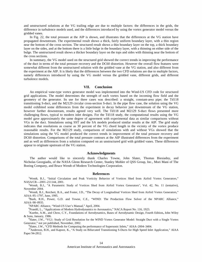
In Fig. 22, the total pressure at the AIP is shown, and illustrates that the differences at the VG station have propagated downstream. The experimental result shows a thick, fairly uniform boundary layer, with a thin region near the bottom of the cross section. The structured result shows a thin boundary layer on the top, a thick boundary layer on the sides, and at the bottom there is a little bulge in the boundary layer, with a thinning on either side of the bulge. The unstructured result shows a thicker boundary layer on the tops and sides with thinning near the bottom of the cross sections.

In summary, the VG model used on the structured grid showed the correct trends in improving the performance of the duct in terms of the total pressure recovery and the DC60 distortion. However the overall flow features were somewhat different from the unstructured solution with the gridded vane at the VG station, and also different from the experiment at the AIP. It is likely that the differences between the two CFD solutions are due to multiple factors, namely differences introduced by using the VG model versus the gridded vane, different grids, and different turbulence models.

VII. Conclusion An empirical vane-type vortex generator model was implemented into the Wind-US CFD code for structured

grid applications. The model determines the strength of each vortex based on the incoming flow field and the geometry of the generator. Its use for three cases was described: a straight, constant-area pipe; the Td118 transitioning S-duct, and the M2129 circular cross-section S-duct. In the pipe flow case, the solution using the VG model exhibited some differences from the experiment in decay behavior just downstream of the VG station, however further downstream, results agreed very well. The Td118 and M2129 S-duct flows presented more challenging flows, typical to modern inlet designs. For the Td118 study, the computational results using the VG model gave approximately the same degree of agreement with experimental data as similar comparisons without VGs in the duct. Simulations using SST and the SA models produced similar results at the AIP. The grid study indicates that resolutions as coarse as 30 percent of the VG chord length in the vicinity of the vortex produce reasonable results. For the M2129 study, comparisons of simulations with and without VGs showed that the simulations using the VG model produced the correct trends in improvement of the total pressure recovery and DC60 distortion. Comparisons of the total pressure contours at the AIP illustrated differences from the experiment and as well as differences from a solution computed on an unstructured grid with gridded vanes. These differences appear to originate upstream of the VG station.

Acknowledgments The author would like to sincerely thank Charles Towne, John Slater, Thomas Biesiadny, and

Nicholas Georgiadis, of the NASA Glenn Research Center, Stanley Mohler of QSS Group, Inc., Mori Mani of The Boeing Company, and Bruce Wendt of Modern Technologies Corporation.

References 1Wendt, B.J., “Initial Circulation and Peak Vorticity Behavior of Vortices Shed from Airfoil Vortex Generators,”

NASA/CR—2001–211144, 2001. 2Wendt, B.J., "A Parametric Study of Vortices Shed from Airfoil Vortex Generators", Vol. 42, No. 11 (tentative),

November 2004. 3Wendt, B.J., Reichert, B.A., and Foster, J.D., “The Decay of Longitudinal Vortices Shed from Airfoil Vortex Generators,”

AIAA–95–1797, June, 1995. 4Bush, R.H., Power, G.D. and Towne, C.E., “WIND: The Production Flow Solver of the NPARC Alliance,”

AIAA–98–0935. 5NPARC Alliance, “Wind-US User’s Manual,” April, 2004. 6Prandtl, L., “Applications of Modern Hydrodynamics to Aeronautics,” NACA Report No. 116, 1923. 7Kuethe, A.M., and Chow, C.Y., Foundations of Aerodynamics, Bases of Aerodynamic Design, Fourth Edition, John Wiley

& Sons, January, 1986. 8Slater, J.W., “VG1: Study of Grid Resolution for the WIND Vortex Generator Model: Straight Duct with a Single Vortex

Generator,” not yet published, November, 2002. 9Slater, J.W., “CFD Methods for Computing the performance of Supersonic Inlets,” AIAA–2004–3404. 10Anderson, B.H., and Kapoor, K., “A Study on Bifurcated Transitioning S-Ducts for High Speed Inlet Application,” AIAA

Paper 94-2812.


15

11Wendt, B.J., and Dudek, J.C., “Development of Vortex Generator Use for a Transitioning High-Speed Inlet,” Journal of Aircraft, Vol. 35, No. 4, July 1998.

12Allan, B.G.; Yao, C.-S. and Lin, J.S., “Numerical Simulations of Vortex Generator Vanes and Jets on a Flat Plate,” AIAA 02–3160, June, 2002.

13Mohler, R.S., “WIND-US Flow Calculations for the M2129 S-Duct Using Structured and Unstructured Grids,” NASA/ CR—2003-212736.

14AGARD Fluid Dynamics Panel, Working Group 13, “Air Intakes for High Speed Vehicles,” AGARD–AR–270, September, 1991.

15Anderson, B.H., and Gibb, J., “Vane Effector Installation Studies on Steady State and Dynamic Inlet Distortion,” AIAA–1996–3279.

-

V max

α

δ

c

h

Figure 1. Vortex generator model parameters.

Vortex G t

Vortex G t

Vortex G t

Vortex G t

Vortex Generator

Leading Edges

Vortex Generator

Trailing Edges

A-A

FLOW

A

A

FLOW

A

A

A

A

Figure 2. Schematic of a counter-rotating arrangement of vane-type vortex generators in a pipe. (Top) Cut-away view of vortex generators in the cylindrical duct. (Bottom)Cross plane view showing generators and the direction of rotation of the shed vortices.

Figure 3. A portion of the geometry and the computational mesh for the pipe flow simulations with the gridded vane, illustrating the fine grid (grid A000) resolution downstream of the VG.


16

Figure 5. Peak vorticity in the pipe with the gridded vane for simulations using the fine grid with the SA and SST models.

0

5000

10000

15000

20000

25000

30000

35000

40000

0 5 10 15 20Axial Distance, x/c

Peak

Vor

ticity

, 1/s

ExperimentSASST

Figure 6. Ratio of transverse to streamwise kinetic energy in the pipe with the gridded vane for simulations using the fine grid with the SA and SST models.

0

0.002

0.004

0.006

0.008

0.01

0.012

0.014


(Tra

nsve

rse

KE)

/(Str

eam

wis

e K

E) ExperimentSASST

Figure 4. Mach contours in the constant area pipe using gridded vane VGs for simulations computed on the fine grid using the SA and SST turbulence models, compared with experimental velocity contours.3(Note that in the views shown, the initial location of the experimental vortex is approximately 10 degrees clockwise of the initial location specified in the CFD simulations.)

SA

SST

x/c = 1 x/c = 5 x/c = 10 x/c = 15x/c = 1 x/c = 5 x/c = 10 x/c = 15

Experiment


17

Figure 7. Transverse momentum vectors superimposed with turbulent viscosity contours for the simulations using the gridded vane.

Figure 8. Mach contours in the constant area pipe using the VG model for simulations computed on the fine grid using the SA and SST turbulence models.

SA

SST


18

VG-Array

Figure 11. Geometry of the td118 transitioning S-duct diffuser and accompanying VG array.

Figure 9. Peak vorticity in the pipe for simulations for using the gridded vane and VG model on the fine grid with the SA model.

0

5000

10000

15000

20000

25000

30000

35000

40000


Peak

Str

eam

wis

e Vo

rtic

ity, 1

/s ExperimentVane, Coarse GridVane, Fine GridModel, Coarse GridModel, Fine Grid

Figure 10. Ratio of transverse to streamwise kinetic energy for simulations using gridded van and VG model on the the fine grid with the SA model.

0

0.002

0.004

0.006

0.008

0.01

0.012


(Tra

nsve

rse

KE)

/(Str

eam

wis

e K

E) ExperimentVane, Coarse GridVane, Fine GridModel, Coarse GridModel, Fine Grid


19

A000: dy = dz = 0.10

B000: dy = dz = 0.15

A011: dy = dz = 0.20

C011: dy = dz = 0.30

Figure 12. Cross plane grids with various resolutions at the axial station where the VG model is applied.

Figure 13. DC60 distortion computed on grid A000 and A111 using both the SA and SST turbulence models.

0

0.01

0.02

0.03

0.04

0.05

0.06

0.4 0.5 0.6 0.7 0.8 0.9 1Dimensionless Radius, r/R

Circ

umfe

rent

ial R

ing

Sect

or

Dis

tort

ion

ExperimentRNS3DWIND SA, Grid A000WIND SST, Grid A000


20

Turb Visc

SA SST

Figure 14. Vorticies on cowl surface illustsrated with turbulent viscosity contours superimposed with transverse momentum vectors for simulations with the SA and SST turbulence models. (Computed using grid A000.)

Figure 15. DC60 ring sector distortion computed on grids with varying resolution.

(a) Cross Stream Resolution

0

0.01

0.02

0.03

0.04

0.05

0.06


Circ

umfe

rent

ial R

ing

Sect

or

Dis

tort

ion

ExperimentA000, dy=dz = 0.10B000, dy=dz-0.15A011, dy=dz=.20B011, dy=dz=0.30

(b) Axial Resolution

0

0.01

0.02

0.03

0.04

0.05

0.06


Circ

umfe

rent

ial R

ing

Sect

or

Dis

tort

ion

ExperimentB000, dx = 0.10C000, dx = 0.15B100, dx = 0.20C100, dx = 0.30

(c) Isotropic Resolution

0

0.01

0.02

0.03

0.04

0.05

0.06


Circ

umfe

rent

ial R

ing

Sect

or

Dis

tort

ion

ExperimentA000, dx=dy=dz = 0.10C000, dx=dy=dz=0.15A111, dx=dy=dz=0.20C111, dx=dy=dz=0.30


21

Experiment A000 (SA)

A000 (SST) A111 (SST)

B000(SST) B011(SST)

B100 (SST) C000 (SST)

C100 (SST) C111 (SST)

Figure 16. Mach number contours on each of the computational grids.


22

Figure 18. Structured computational mesh used for Wind-US computations with VG model.13

Figure 17. Schematic of M2129 S-duct.13

throat

“engine face”

vane vortex generators

Figure 19. Total pressure recovery in the M2129 S-duct.

0.9500.9550.9600.9650.9700.9750.9800.9850.9900.995

0.3 0.4 0.5 0.6 0.7 0.8 0.9Throat Mach Number

Tota

l Pre

ssur

e R

ecov

ery Baseline

VG170

(a) Experiment (b) Wind-US Unstructured

0.9500.9550.9600.9650.9700.9750.9800.9850.9900.995


Tota

l Pre

ssur

e R

ecov

ery Baseline

Gridded Vanes

(c) Wind-US Structured.

0.9500.9550.9600.9650.9700.9750.9800.9850.9900.9951.000


Tota

l Pre

ssur

e R

ecov

ery Baseline

VG model


23

(a) Structured solution using VG model.

(b) Unstructured solution using gridded vanes.

Figure 21. Mach number contours at VG trailing edge in M2129 duct.

Figure 20. DC60 distortion at the AIP of M2129 S-duct, shown with and without configuration VG170.Comparisons are of experimental data, and WindUS simulations on an unstructured grid with gridded vane VGs, and on a structured grid using the VG model.

0

0.1

0.2

0.3

0.4

0.5

0 0.2 0.4 0.6 0.8 1Throat Mach Number

DC

60

ExperimentUnstructuredStructuredE i t


24

Experiment Unstructured Solution with Gridded Vane

Structured Solution with VG model

Figure 22. Total pressure contours at the AIP for the M2129 S-duct.

An Empirical Model for Vane-Type Vortex Generators in a ... · American Institute of Aeronautics...

Documents

Transcript of An Empirical Model for Vane-Type Vortex Generators in a ... · American Institute of Aeronautics...