NASA Contractor Report 198501MAA-96--0807

The Modelling of Symmetric AirfoilVortex Generators

B.J. Wendt

Modern Technologies Corporation

Middleburg Heights, Ohio

and

B.A. Reichert

Kansas State UniversityManhattan, Kansas

June 1996

Prepared forLewis Research Center

Under Contract NAS3-27377

NaUonalAeronautics andSpace Administration

https://ntrs.nasa.gov/search.jsp?R=19960027051 2018-06-16T21:59:46+00:00Z

THE MODELLING OF SYMMETRIC AIRFOIL VORTEX GENERATORS

B. J. Wen& °,

Modern Technologies Corporation, Middleburg Heights, Ohio, 44130B. A. Reichert*

Kansas State University, Manhattan, Kansas, 66506

Abstract aircraft inlet in Figure 1. In internal flows, vortex genera-

tors are used to prevent excessive boundary layer growth,

flow separation, and to reduce total pressure distortion ofthe airstream ingested by the aircraft engine. These ef-

fects occur readily in inlet ducts and diffusers due to suchfactors as duct centerline curvature, and large streamwise

variations in duct cross-sectional area.

An experimental study is conducted to determine the

dependence of vortex generator geometry and impingingflow conditions on shed vortex circulation and crossplane

peak vorticity for one type of vortex generator. The

vortex generator is a synm_tric airfoil having a NACA

0012 cross-sectional profile. The geometry and flow

parameters varied include angle-of-attack a, chordlength

c, span h, and Mach number M.

The vortex generators are mounted either in isolation

or in a symmetric counter-rotating array configurationon the inside surface of a straight pipe. The turbulent

boundary layer thickness to pipe radius ratio is 6/R

0.17. Circulation and peak vorticity data are derived fromcrossplane velocity measurements conducted at or about

1 chord downstream of the vortex generator trailing edge.

Shed vortex circulation is observed to be propor-

tional to M, a, and h/6. V_qth these paran_ters heldconstant, circulation is observed to fall off in monotonic

fashion with increasing airfoil aspect ratio AR. Shed vor-

tex peak vorticity is also observed to be proportional toM, _, and h/6. Unlike circulation, however, peak vor-

ticity is observed to increase with increasing aspect ratio,

reaching a peak value at AR _ 2.0 before falling off.

Introduction

Vortex generators are often used in a variety of

fluid engineering applications where a small, but critical,amount of flow control is necessary for proper flow com-

ponent performance.Common uses are in aircraft systemswhere surface-mounted vortex generators are applied in

external (airframe related) and internal (propulsion re-

lated) flows. Figure 1 depicts a typical application of

surface-mounted vortex generators. In external flow sit-

uations, such as that encountered on the wing surface in

Figure 1, the most common arrangement is array forma-

tions upstream of flight control surfaces where boundary

layer attachment is often critical to flight performance.

An array of vortex generators is also being used in the

*Research Engineer, 7530 Lucerne Drive, Islander

Two, Suite 206, Member AIAA

*Associate Professor, Department of Mechanical En-

gineering, 302 Durland Hall, Member AIAA

Figure 1 Flow conditioning with vortex generators.

The key to vortex generator performance is in the

mixing and secondary velocity field created downstream

by the shed vortex structures. If properly situated inthe flowfield, the helical motion of the fluid in the vor-

tex forces high energy fluid of the freestream or coreflow into the slower moving fluid of the boundary layer.

The re-energized boundary layer fluid is now more re-

sistant to flow separation. Vortex generator induced flow

may also be used to counter boundary layer thickening

due to component-generated secondary flows. Recent

experimental work in an S-duct 1 and a rectangular-to-semiannular diffuser 2 have demonstrated the effective-

ness of this approach.

The large number of parameters to consider when

designing a vortex generator array for an aircraft com-

ponent (such as the wing or inlet illustrated in Figure1) has the implication that experimental work to achieve

optimum performance is often slow and expensive. Thisfact has motivated a few workers in computational fluid

mechanics to assist in the optimizing process by includ-

ing a means of representing vortex generators in their

codes. A simple and effective way of doing this is to

employ a model for the crossplane velocity or vorticityfield induced by the vortex generators. This is the ap-

proach taken in recent work by Anderson et al. 3"4 who

examined multiple vortex generator array geometries in a

diffusing S-duct inlet using a parabolized Navier-Stokes(RIGS) solver. A similar inclusion of embedded vortices

in a full Navier-Stokes (FNS) code was implemented byCho and Greber s for a constant area circular duct and a

diffusing S-duct geometry.

The advantage to modelling the crossplane velocity

or vorticity distribution induced by the vortex generator is

that a simple exponential expression accurately captures

the crossplane velocity or vorticity distribution of the shedvortex. To demonstrate this, consider Figure 2. Figure

2 illustrates the secondary velocity field of an embedded

vortex (data on the left,model on the right) shed from an

airfoil-type vortex generator. This vortex generator is one

of 12 symmetrically placed vortex generators spanningthe inside circumference of a straight pipe. The data is

acquired in the crossplane one chord length downstream

of the vortex generators. The model is constructed froma summation of 24 terms (12 embedded vortices plus 12

image vortices) each having the form6:

[Lt-exp\ I'_ ] '

where Fi is the measured circulation of the ith vortex or

image, w_"_ is the measured peak or maximum valueof the induced streamwise vorticity field, and P_ is the

measured crossplane location of the vortex center. These

quantifies are known as "vortex descriptors" followingthe work of Russell Westphal 7. Any such model requires

a description of the vortex strength (here Fi) and concen-

tration (here a,_ _, but viscous core radius, re_, is another

possibility). Tim model above is based on the classical"ideal viscous" or Oseen vortex, s

Many studies have demonstrated the remarkablesimilarities between the Oseen-based model and the cross-

plane structure of embedded vortices shed from vortexgenerators. Pauley and Eaton 9 demonswated this in a

study of delta wing vortex generators, Wendt et al. to in a

study of blade-type vortex generators, Wendt and Hingst s

for low-profile wishbone vortex generators, and more re-cently, Wendt eta/. 6 on symmetric airfoil-type vortex

generators.

To complete the modelling of a vortex generator we

must now show how the descriptors of the model vor-

tex depend on downstream axial position, the geometry

of the vortex generator, and impinging flow conditions.

For airfoil-type vortex generators we might express this

dependence as:

r = r(z, c, h, ,,,profile, 6, M, Re, ...),

w "n'x = w'_(z,c, h, a, profile, 6, M, Re, ...),

R = R(z, c, h, a,profile, 6, M, Re, ...),

(2)

where "profile" refers to the shape of the airfoil, z is

the axial position (measured from the trailing edge of the

vortex generator), c is the chord length, h is the span,

a is the angle-of-attack, 6 is the boundary layer thick-ness of the impinging stream, M is the freestream or

core Mach number and Re is a Reynolds number. The

vortex generator models in use at the present time only

crudely approximate the functional dependence indicated

in Equation 2. As a means of improving current vortex

generator models this study was undertaken to examinethe effect of vortex generator geometry and impinging

flow conditions for one type of symmea'ic airfoil vortex

generator (NACA 0012). This paper reports the results

of a series of experimental tests covering a range of vor-

tex generator h/c (or "aspect ratio"), h/6, a, and M.The vortex generators are mounted either in isolation on

the inside surface of a straight pipe, or in a symmet-

ric counter-rotating array spanning the full circumference

of the pipe. Duct or pipe core flow conditions are sub-sonic with a nominal boundary layer thickness to pipe

diameter ratio, 6/D = 0.09. Three-dimensional mean

flow velocity data are acquired in a crossplane grid lo-

cated approximately one chordlength downstream of the

vortex generator model(s). This is done using a rake of

O degrees 0 degrees

95 85 95 85

105 _ L._._ ¢_ L_..._

t_ 1 g d# d

,d/2-r)¢_.O_---\i_'..:::'=iiiii!! / (d/2-r, mm _ "'. "_'o_'.._iii_ii i '

:°\: : ,i.3.0 : - :::::::!iiiii:::: • .o ::-.i::::

ta \" 3on_.---> m_.---> 'da mode

4.0"_ 4.0"_

Figure 2 A comparison of the transverse velocity field of an embedded vortex; data on theleft, and a model constructed from the superposition of Oseen vortices on the right.

2

Flow

!_._ Plenum

St& St&0 2.29

= _a- Test Section Duct _--- Exhaust Region-----_

] [ Su_A_p_c

Dimensions in Meters

St& Sta. Sta. St&4.50 5.55 10.14 12.96

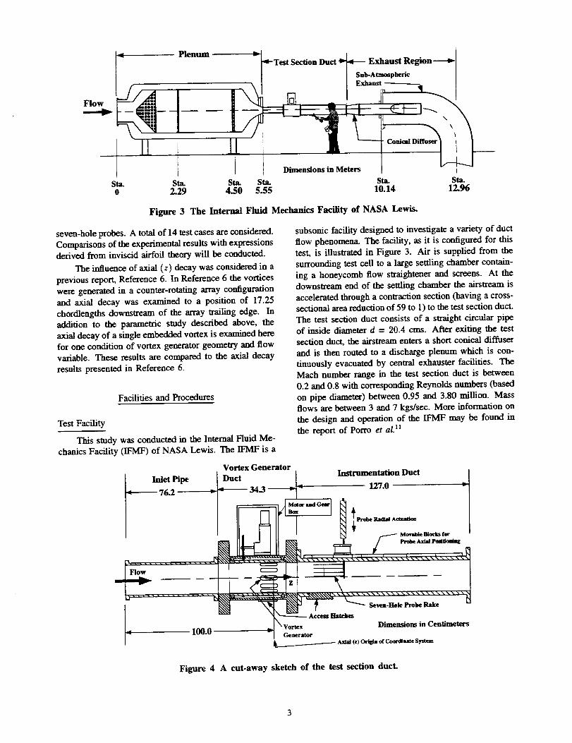
Figure 3 The Internal Fluid Mechanics Facility of NASA Lewis.

seven-hole probes. A total of 14 test cases are considered.

Comparisons of the experimental results with expressionsderived from inviscid airfoil theory will be conducted.

The influence of axial (z) decay was considered in a

previous report, Reference 6. In Reference 6 the vorticeswere generated in a counter-rotating array configuration

and axial decay was examined to a position of 17.25

chordlengths downstream of the array trailing edge. In

addition to the parametric study described above, the

axial decay of a single embedded vortex is examined herefor one condition of vortex generator geometry and flow

variable. These results are compared to the axial decay

results presented in Reference 6.

Facilities and Procedures

Test Facility

This study was conducted in the Internal Fluid Me-chanics Facility (IFMF) of NASA Lewis. The IFMF is a

subsonic facility designed to investigate a variety of duct

flow phenomena. The facility, as it is configured for thistest, is illustrated in Figure 3. Air is supplied from the

surrounding test cell to a large settling chamber contain-

ing a honeycomb flow straightener and screens. At thedownstream end of the settling chamber the airstream is

accelerated through a contraction section (having a cross-sectional area reduction of 59 to 1) to the test section duct.The test section duct consists of a straight circular pipe

of inside diameter d = 20.4 eros. After exiting the test

section duct, the airstream enters a short conical diffuserand is then routed to a discharge plenum which is con-

tinuously evacuated by central exhanster facilities. TheMach number range in the test section duct is between

0.2 and 0.8 with corresponding Reynolds numbers (based

on pipe diameter) between 0.95 and 3.80 million. Massflows are between 3 and 7 kgs/sec. More information on

the design and operation of the IFM may be found in

the report of Porto et al. li

Inlet Pipe

76.2

_ 1_.0Ax_ (z) _ or coo_/S_

Vortex Generator

Duct 34.3 [_ Instrum_7_on Duct _[I

IlL/III

_ .....Z X................--.. ......

v I GeneratOr

Figure 4 A cut-away sketch of the test section duct.

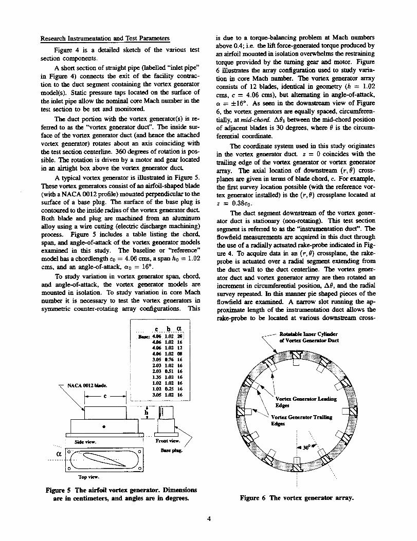
Research Instrumentation and Test Parameters

Figure 4 is a detailed sketch of the various test

section components.

A short section of straight pipe 0abelled "inlet pipe"

in Figure 4) connects the exit of the facility contrac-

tion to the duct segment containing the vortex generator

model(s). Static pressure taps located on the sarface of

the inlet pipe allow the nominal core Mach number in thetest section to be set and monitored.

The duct portion with the vortex generator(s) is re-

ferred to as the "vortex generator duct". The inside sur-

face of the vortex generator duct (and hence the attached

vortex generator) rotates about an axis coinciding with

the test section centerline. 360 degrees of rotation is pos-sible. The rotation is driven by a motor and gear located

in an airtight box above the vortex generator duct.

A typical vortex generator is illustrated in Figure 5.

These vortex generators consist of an airfoil-shaped blade

(with a NACA 0012 profile) mounted perpendicular to the

surface of a base plug. The surface of the base plug iscontoured to the inside radius of the vortex generator ducL

Both blade and plug are machined from an aluminum

alloy using a wire cutting (electric discharge machining)

process. Figure 5 includes a table listing the chord,

span, and angle-of-attack of the vortex generator modelsexamined in this study. The baseline or "reference"

model has a chordiength co = 4.00 cms, a span h0 = 1.02

cms, and an angle-of-attack, cz0 = 16 °.

To study variation in vortex generator span, chord,

and angle-of-attack, the vortex generator models are

mounted in isolation. To study variation in core Mach

number it is necessary to test the vortex generators in

symmetric counter-rotating array configurations. This

Top _¢w.

c h cc__ _4;___bo2___j

4.06 1.02 164.06 1.02 12

&06 1.02 083.05 0.76 16

2.03 1.02 16

2.03 0.51 161.35 1.02 16

1.02 1.02 161.02 0.25 16

3-05 1.02 16

h

Figure $ The airfoil vortex generator. Dimensions

are in centimeters, and angles are in degree_

is due to a torque-balancing problem at Mach numbersabove 0.4; i.e. the lift force-generated torque produced by

an airfoil mounted in isolation overwhelms the restraining

torque provided by the turning gear and motor. Figure

6 illustrates the array configuration used to study varia-

tion in core Mach number. The vortex generator arrayconsists of 12 blades, identical in geometry (h = 1.02

cms, c = 4.06 cms), but alternating in angle-of-attack,

= -4-10°. As seen in the downstream view of Figure

6, the vortex generators are equally spaced, circumferen-

tiatly, at mid-chord. A0b between the mid-chord position

of adjacent blades is 30 degrees, where 0 is the circum-ferential coordinate.

The coordinate system used in this study originates

in the vortex generator duct. z = 0 coincides with the

trailing edge of the vortex generator or vortex generator

array. The axial location of downstream (r, O) cross-

planes are given in terms of blade chord, c. For example,the first survey location possible (with the reference vor-

tex generator installed) is the (r, O) crossplane located at

z = 0.38c0.

The duct segment downstream of the vortex gener-ator duct is stationary (non-rotating). This test section

segment is referred to as the "ins_tafion duct". The

flowfield measurements are acquired in this duct through

the use of a radially actuated rake-probe indicated in Fig-

ure 4. To acquire data in an (r, 0) crossplane, the rake-probe is actuated over a radial segment extending from

the duct wall to the duct centerline. The vortex gener-

ator duct and vortex generator array are then rotated an

increment in circumferential position, AO, and the radial

survey repeated. In this manner pie shaped pieces of theflowfield are examined. A narrow slot running the ap-

proximate length of the instnmmntation duct allows the

rake-probe to be located at various downstream cross-

_ Retatable Inner Cylinder

of Vortex Generator Duct

Figure 6 The vortex generator array.

planes. A series of slot-sealing blocks determines theallowable axial location of survey crossplanes, zi (again

with the reference vortex generator mounted) :

zi = 0.38co, 1.OOco, ..., 10.38co,

14.75co, 15.38co, ..., 24.75co.(3)

The rake-probe consists of 4 seven-hole probe tips

spaced 2.54 cms apart. These probes are calibrated inaccordance with the procedure outlined by Zilliac. 12 The

flow angle range covered in calibration is q-600 in both

pitch and yaw for the probe tip closest to the wall. The

calibration range for the outer 3 tips is approximately

q-30 °. Uncertainty in flow angle measurement is 4-0.7 °

in either pitch or yaw, for flow angle magnitude below

35 degrees (pitch and yaw flow angle magnitude did not

exceed 35 degrees in this study). The corresponding

uncertainty in velocity magnitude is approximately -1-1%

of the core velocity, v_.

The circumferential extent of the crossplane survey

grid is determined by the objectives of the study. InReference 6 we were interested in studying the cross-

plane domain of a single embedded vortex constrainedon either side by its counter-rotating neighbors. The cir-cumferential extent of that domain was 30 degrees as

determined by the geometry of the parent vortex gener-

ator array. Surveying the full 30 degrees allowed us to

determine quantifies such as vortex angular momentumand transverse kinetic energy, in addition to the vortex

core descriptors of circulation and peak vorticity. This

data will again be useful at a later point in this paper

when we attempt an analysis of the present results. Wenote now, however, that acquiring vortex angular momen-

tum or transverse kinetic energy for an isolated embed-ded vortex would involve surveying most, if not all, of

the pipe crossplane, an impractical requirement consider-

ing the crossplane grid resolution employed here. Thus,for most of the present study, we will limit ourselves to

obtaining only the vortex descriptors. These can be accu-

rately measured by a survey grid coveting the near-regionof the vortex viscous core. In most instances this involves

a grid of only 20 or 25 degrees in circumferential extent.

Crossplane grid resolution is based both on the sizeof the vortex core and the time needed to acquire data

with the rake-probe. In most test cases here the axial

location of the survey grid is z = co, the vortex core

is approximately 1 centimeter in diameter, and is highly

concentrated with large secondary velocities present. Suf-ficient resolution is obtained with A0 = 1 ° on the grid

interior, and Ar = 1.3 ram. The vortex core grows insize and becomes more diffuse as it moves away from

the parent vortex generator. Thus for axial locations suf-ficiently far downstream (visited when examining the ax-

ial decay of the single embedded vortex) we can coarsen

the grid described above somewhat, with A0 = 1.50 andAr = 1.7 ram.

Experimental Results

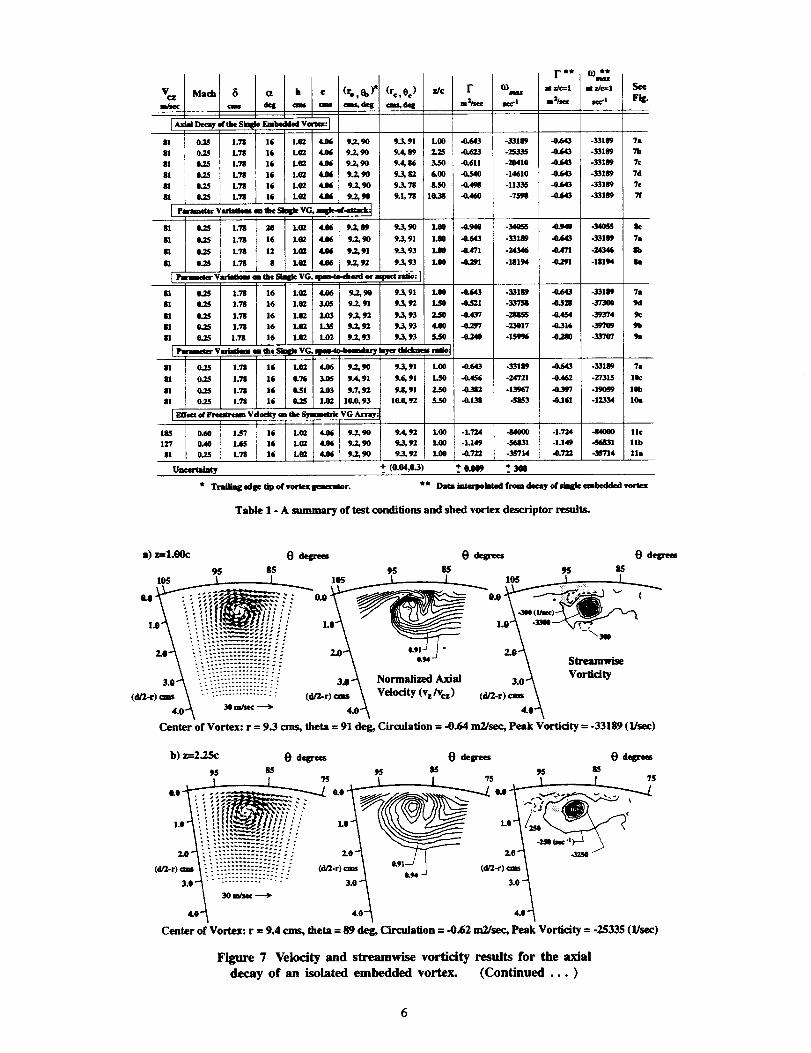
Table 1 and Figures 7ml 1 summarize the results

of this study. Table 1 lists the test conditions for every

crossplaae illustrated in Figures 7--11, and tabulates the

vortex descriptors determined for each crossplane of data.The vortex descriptors are also included in Figures 7--11.

In Figures 7--11 the radial axis represents distance fromthe wall, in centimeters, and the circumferential axis

represents angular position in degrees. The axial position

of each crossplane is indicawxl. Note again that this is

given in chordlengths of the model being tested and ismeasured from the trailing edge tip of the airfoil.

The vortex descriptors originate from the transverse

velocity data in the crossplane. The vector plots onthe left hand side of Figures 7--11 are the measured

transverse velocity data. The transverse velocity data is

first converted to streamwise vorticity data following the

relation:6vo vo 1 6v_

wz = _ + (4)r rtO'

where (v_, vo ) are the transverse components of velocityin the radial and circumferential coordinates, respectively.

Finite difference formulas are used to represent the spatial

derivatives in Equation 4. The resulting streamwise vor-

ticity fields are plotted on the right hand side in Figures7--11. Solid contour lines represent negative or "core"

vorticity, dashed lines are positive or "secondary" vortic-

ity. The contour increment for solid lines not labelled is-3000 see -x. Wmar is located at some grid point having

coordinates (re, 0r). The vortex circulation r is calcu-

lated by first isolating the region of core vorticity in thedata field. This is done by referring to the contour plots

of vorticity in Figures 7--11. A path enclosing the re-

gion of core vorticity is defined. The outer boundary ofthe core is taken to be the location where streamwise vor-

ticity is 1% of w,,_a_. The circulation is then calculated

according to:

f V.ds,

path

(5)

where V is the velocity vector in the crossplane, and

s refers to the path coordinate. By using closed paths

composed of line segments in the r or 0 coordinate di-rections the circulation is easily determined. Uncertainty

estimates for all listed descriptors are given in Table 1.

These are derived by combining the uncertainties in mea-

sured velocities and probe placement in accordance with

the procedure outlined by Moffat.t3

Vcz

R

[A_Ud_,ra. S_ -.,_m,d v_.: I

81 0.2.5 1.78 16 L02 4.06 9.2, 90

81 0.25 1.78 16 L02 4.06 9.7, 90

81 0.25 1.78 16 L_ 406 9.2, 90

81 0.25 1.78 16 L92 4._ 9.2, 90

m ,.zs LTs 16 L92 4_ 9_._0m oas LTs l_ L,z ¢0, 9.z,90

81 0.25 1.78 20 LO2 4.06 9.2, 89

81 0.25 1.78 16 L02 4.06 9.2, 90

81 0.25 1.7'8 12 L02 406 9.2, 91

81 0.2S 1.78 8 La2 4.06 9.2, 92

9-3, 91 LO0 -0.643

9.4, 89 _ -4..623

9.4, 86 3.5O -0.611

9.3, 82 _,00 -0.S4O

9.3, 78 8J,0 `0.49g

9.1,78 10.38 -0.460

9.3, 5q) L00 `0._

9.3, 91 L00 `0.643

9.3, 93 1.00 -0.471

9.3, 93 1.00 `0._1

I _ Varimobm m ebe Siqle VG, _ord or mq_ect ndio:

81 0.25 1.78 16 LG2 4.06 9.2, 90 9.3, 91 L00 -0.643

81 0.25 I.TS 16 LQ2 _05 I 9.2, 91 9.:3, 92 1.50 `0.521

81 0.25 1.78 16 L_ 203 I 9.2, 92 9,.3,93 _ -0.437

81 0.25 1.78 16 L62 1._ 9.2, 92 9-3, 93 4.00 -0.297

m _ l._ ]6 1.02 !.02 9_yJ 9_93 s.soI Pm'sme_ Y_ em the Sbq_e VG' _ ImT_rtldckn_ mJ°

81 0.25 1.79 16 L62 406 9.2, 90 9.3, 91 L00 -0.643

81 0.25 1.78 16 0.76 3.05 9.4, 91 9.6, 91 1.50 `0.456

81 0.25 1.78 16 0.51 203 9.7, 92 9.L 91 2.50

81 0..25 1.78 16 0._ 1.02 10.0, 93 10._ 92 S.SO ..0.138

[ Effect _r Fnmmmmm V dodty on tide SymJu_'k VG An'By:

185 0.60 l.b'7 16 I 1.0_ 4.06 9.2, 90 9.4, 92 L00 -1.724

127 0.40 1.65 16 [ L0_ 4.06 9.2., 90 9.3, 92 L00 -L14981 0..25 L7S 16 L mo 4.06 9.2, 90 9.3, 92 L00 ..0.722

Unem'mi_ +. (0.04,0.3) +

See

Fig.

-33189 -0.643 -33189 78

-253_ -0.643 -33189 7"o

-20410 -0.643 ,-33189 7c

-1461O -0.643 -33189 7d

-113_ `0.643 -33189 7e

-759$ -0.643 -33189 7f

-340_ -0.940 -MOSS 8¢

-33189 -0.643 ..33189 7s

-2_J6 -0.471 -24346 8b

-18194 `0.291 -18194 t.

-33189 -0.643 -33189 78

-337_ -0.528 -373OO 9d

-28_5 -0.454 -,39374 9c

-23017 `0.316 ..tlP709 9b

.159_6 -4,,280 -M707 9a

-331a9 -0.643 -331,119 7s

-24721 -0.462 -2731.5 il01:

-13967 -0.397 -19059 106

-5853 -0.161 -123M lee

•414000 .!.724 -84000 llc

-_6831 -I.149 ..56831 lib

-35714 ..0.722 -36"714 Ila

+.3OO

* Tmil_edp61pofvortexl_aerator. ** D_interpolatedfrem6ec_ofslmgleembeddedvoctex

Table 1 - A summary of test conditions and shed vortex descriptor results.

a) z:=l.00c O degrees e degrees 0 degrees

9_ 8.5 9S 8.5 95 8_

1.8 .;;',' _ ,_ LO 1.0

3.0 \i -iiiiiiiiir-i// 3.o Norm i dAxi Vor aty

4.0 "_ 30 m/see -_ 4.0 "_ 4.0"_

Center of Vortex: r = 9.3 cms, theta = 91 deg, Circulation = -0.64 m2/sec, Peak Vorticity = -33189 (1/sec)

b) z=225c O degrees 0 degrees 0 degrees

95 85 95 85 95 85

L.._ ,_..._l L__ ?

\ _0 m/sec '--_

Center of Vortex: r = 9.4 cms, theta = 89 deg, Circulation = -0.62 m2/sec, Peak Vorticity = -25335 (1/sec)

Figure 7 Velocity and streamwise vorticity results for the axialdecay of an isolated embedded vortex. (Continued ... )

C) Z-_-3.50C 0 degrees 0 degrees 0 degrees

95 85 95 85 95 85

-t 't_o- i i_.iiii_i.---.--'.-:_i_/// 2.o- ,,____r " t ._.n

(d/2-r)cms i - :-:::::-"-"-.".:.-'.-'--:.:-: (d/2-r) cms 0.94-_ (d/_r) cms /

3.0"30 m/sec

4.0 4.0

Center of Vortex: r = 9.4 cms, theta = 86 deg, Circulation = -0.61 m2/sec, Peak Vorticity = -20410 (1/sec)

d) z=6.00c85

0.0

1.0

(d/2-r) cms

2.0-

3.0-

4.0-

0 degrees

0.0-

• , #i# _ _ x, ,, . .

...... _# _ , .

:: i "- ."i - -"-"-".".-"-:::L:?: ::" 3.0-

30 m/sic -----_4.0-

0 degrees85

\t,t <__,__2.0-

0.91_ l 3.0--0.94_

4.0--

0 degrees85

"1_ (tuec't) _3154D _

Center of Vortex: r = 9.3 cms, theta = 82 deg, Circulation = -0.54 raMs°c, Peak Vorticity = -14610 (l/sec)

e) z=&50c85

LO - ___

LO-

(dt2-r) cms

2.°-

3.0-

4.0- 30 m/see

7? 0 degrees e.e-

1.°-

(d_.-r) ¢ms

_1/// /'/ /'.." 2.o_

.:-//:.'.: 3.0-

4.°-

85

o.ll _ &O -

&°-

&S

_75 e degrees

-

Center of Vortex: r = 9.2 cms, theta = 78 def. Circulation = -0.50 m2/sec, Peak Vorticity = -11335 (1/sec)

t.O-

l.O-

(d/2-r) am

2.0-

3.0-

4.0-

75 O degrees. -

O0

65

. . . 2...__11,,',,,...., .::'"-::':s,:..'..'." 2o-

: ": : : _-: :-: : :':.".'."." 3.0-

:::::i-:.::.:-././.'..(<_l-,)--........ - "" "" " "'-""-" 4.0-

30mtse¢----_ o°." --."

85

eg_ _ e._ -_ (cgZ-r) ms

4.°-

85

Center of Voi'tex: r= 9.1 cms, theta= 78 deg, Circulation = -0.46 m2/sec, Peak Vorticity = -7598 (1/sec)

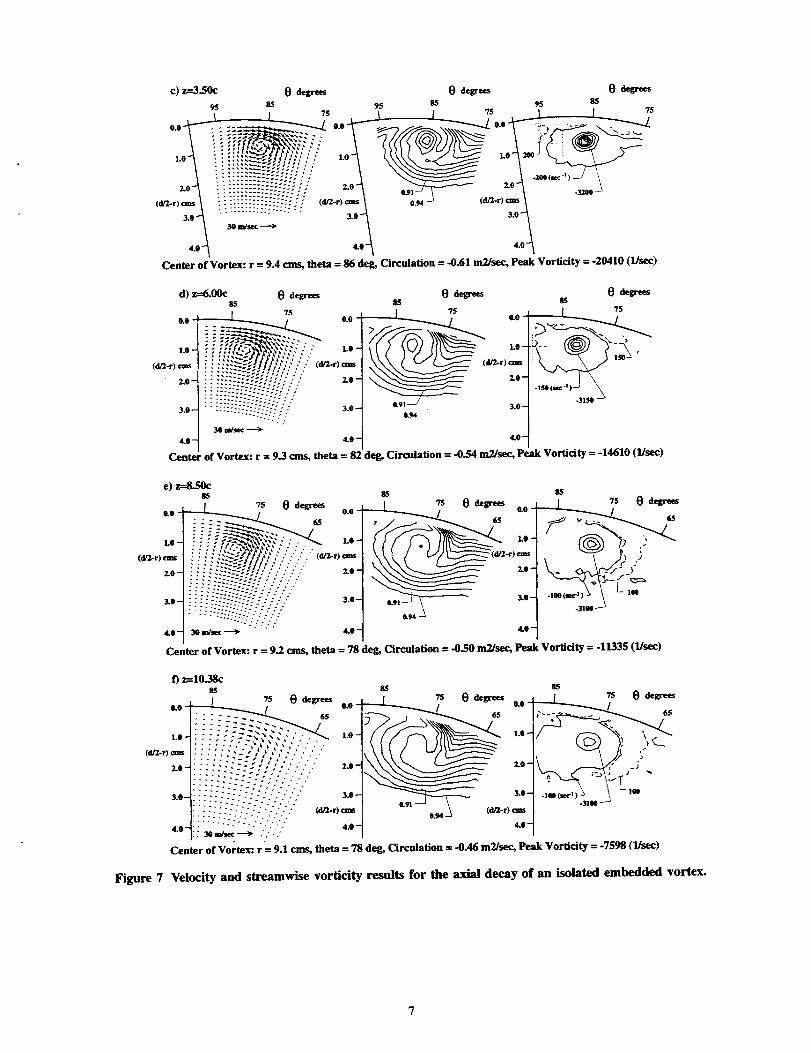
Figure 7 Velocity and streamwise vorficity results for the axial decay of an isolated embedded vortex.

a) alpha=8 deg, z=l.00c 0 degrees 0 degrees 0 degrees

95 85 95 85 95 85

lo5_ I los _ _ lOS

\

iiiiiiJH////-\_-i:il;ii;iil;i!// _0

(d/2-r) cI \ ................... (d/2-r) cms \ (dt2-r) ares \

Center of Vortex: r = 9.3 cms, theta = 93 deg, Circulation = -0.29 rn2/sec, Peak Vorticity = -18193 (l/sec)

b) alpha=12 deg, z=l.OOc 0 degrees 0 degrees 0 degrees

95 85 95 85 95 85

..o\ iiiiii -/.\ - ,o-.,::5,o_.- _-_-. .oi ,01

Center of Vortex: r = 9.3 cms, theta = 93 deg, Circulation = -0.47 m2/sec, Peak Vorticity = -24346 (1/sec)

c) alpha=20 deg, z=l.00c O degrees e degTees 0 degrees

9S 85 95 85 95 85

Center of Vortex: r = 9.3 cms, theta = 90 deg, Circulation = -0.94 m2/sec, Peak Vorticity = -34055 (1/see)

Figure 8 Velocity and streamwise vorticity results for variation in airfoil angle-of-attack.

a) AR--2.546, _-5.50c 0 degrees e degrees e degrees

95 85 95 g.5 95 8,5

o.o_V,-_iii_-_iiii.".-_ - _o_'V_ _o_'_-__d_ _--

-f ::::::::::::::::::::::::,.0_ _,\"_iii!;ii!!ii_ii/ ,.o1 ,.01

(d/2-r) _ms \ -" "............. (dt2-r) cms \ (dr2-r) cms \

4.0"_ _om_ _ ,0"_ 4.o-_Center of Vortex: r = 9.3 cms, theta = 93 deg, Circulation = -0.24 m2/sec, Peak Vorticity = -15996 (1/sec)

Figure 9 Velocity and streamwise vorticity results for variation in airfoil aspect ratio. (Continued...)

b) AR=I.910, _-4.00c 0 degrees 0 degrees 0 degrees

95 85 95 85 95 85

1o5/ los _.l _ los

' •• ::::::::::::::::::::::::::::// 3.0

(d/Z-r ":::::'"':::: " " (d/2-r (dJ2-r

_.o-_ _o_-_ ,o-_ _.o-_Center of Vortex: r = 9.3 cms, theta = 93 deg_ Circulation = -0.30 nL?Jsec,Peak Vorficity = -23017 (l/sec)

c) AR=l,?73, z=2.50c 0 degrees 0 degrees 0 degrees

95 85 95 85 95 85

.._'_-_,'D_i_//: , ,o

:-::.-:_:.----:::::::-:-:=---_-:-:---:!i_! / .- _'_ io__:\ --:--:.=.'".!i: :-: : - 3.03.0"_

Cente_of Vortex: r = 9.3 cms,theta= 93deg,Circulation = -0.44 m2/sec,Peak Vortlcity = -2,8855(llsec)

d) AR---0J]49, z=l__0c 0 degrees O degrees 0 degrees

95 85 95 85 95 85

o.o____-_=--o.o_-_-___ -o.o_f.__ •

..........:oi ol-,i!_!ii77//ii/ _ '-"-7.__)

_i _ _ (d/i-r) (d#2-r

Center of Vortex: r = 9.3cnis, ihela = 92d_ Circulaiion = -0._2mi#sec,Peak Vorlicity = -33758 (l#sec)

Figure 9 Velocity and streamwise vorticity results for variation in airfoil aspect ratio.

a) h---0.25 cms, z:=5.50c 0 degrees 0 degrees 0 degrees

95 85 95 85 95 85

I_ 105 _ 105

o.0 .__:i!!i!!ili;i/// _ _ _ "'-"._,,_1.o -,. ttii!!::::::iii!ii7/ / i.o _.o

_.o_ _.o-_(d/2-r 3.0 '':':: :::::::::"" (dr2-r)c_ \ (d/2-r)ms \

4.0A 30 m/sec ----_ 4.0"_ 4.0"_

Center of Vortex: r = 10.0 cms, theta = 92 deg, Circulation = -0.14 m2/sec, Peak Vorticity = -5853 (l]sec)

Figure 10 Velocity and streamwise vorticity results for variation in

airfoil span-to-boundary layer thickness ratio. (Continued...)

b) h=O..51 cms, z=2.50c 0 degrees 0 degrees 0 degrees

95 85 95 85 95 85

los_ L__ 10s _1 L__ los _J I_

\ . " i:.'::':':.':!:.'::::: . I \ _ _-'_"----'- 1._ "1_")-_ -3_s*_1. \ : --i:._:::::::_i!.: - - • • "

(da-r)eros \ (da-r)c_ \ (d_r)_ \4.0_ 30 m/see _ 4.0_ 4.0"_

Center of Vortex: r = 9.8 cms, theta = 91 deg, Circulation = -0.38 m2/sec, Peak Vorticity = -13967 (1/sec)

c) h=0.76 cms, z=l.50c 0 degrees O degrees 0 degrees

95 85 95 85 95 85

(d/2-r) cms \ (d/2-r) cms \ (d/g-r) ¢_s \

Center of Vortex:. r = 9.6 cms, theta = 91 deg, Circulation = -0.46 m2/sec, Peak Vorticity = -24721 (llsec)

Figure 10 Velocity and streamwise vorticity results for variation in airfoil span.to.boundary layer thickness ratio.

a) Mach---O.25, z=l.OOc O degrees 0 degrees 0 degrees

95 85 9_ 85 95 8510s __--------._ 10s _L L__ los

0.0 . -" : : 0.0 _ _ 0.0 ....* ~ "" .

3.0"_ 3.0_ 3.0"_

• 4.o- Center of Vortex: r = 9.3 cms, theta = 92 deg, Circulation = -0.72 m2Jsec, Peak Vortidty = -35714 (lJsec)

b) Mach=0.40, z=l.OOc 8 delpees O degrees O degrtes

95 85 95 85 95 85105 _ J._.. 105 _ 105

"°) "/" / I ,.o 1.o

"."__.i i""::'--'--_;" '"------- ,, _ -,-_ _o_ ..,.,,_

2.0 ,, : :..::_:_ .... , 2.0•. , .--: ........ "..';,,

3.0 ":-::::'7::::::::: ": _o_ 3.o"_(d/2-r (d/2-r) -- \ (d/2-r)-- \

4.0A 30 "_c ---'_" 4.0"_ 4.0"_

Center of Vortex: r = 9.3 cms, theta = 92 deg, Circulation = -1.15 m2Jsec, Peak Vorticity = -56831 (1/sec)

Figure 11 Velocity and streamwise vorticity results for variation in core Mach number. (Continued ... )

10

c) Mach--0.60, z=l.OOc 0 degrees 0 degrees 0 degrees

95 85 95 85 95 85

.._ los los

....::::..... : (d/2-r)clas \ ( " )

30 mi_c --'--'_ 4.0 "_ 4.0"_

o.o ,o\

\

3.o iii::....

4.0"_

Center of Vortex: r -- 9.4 cms, theta = 92 deg, Circulation = -1.72 m2dsec, Peak Vorticity = -83999 (l/sec)

Figure 11 Velocity and streamwise vorticity results for variation in core Mach number.

Contours of primary velocity ratio, v_/vcz, are pro-

vided in the middle plots of Figures 7--11. Vcz is the

core velocity of the pipe and is listed in Table 1. Anadditional feature of the plots in Figures 7--11 is the in-

clusion of the crossplane profile of the vortex generator

on the plots of streamwise vorticity (shaded region). Thecomer marked with the dashed cruciform is the trailing

edge tip.

Table 1 is organized into groupings of test cases cov-

ering 5 variations in test conditions. The first four group-ings examine variation in z, a, aspect ratio, and h/6.

Figure 7a, the single embedded vortex at z = 1 chordand shed from the reference vortex generator, is common

to all 4 groupings and is thus referred to as the "baseline"test case. This is indicated in Table 1. The fifth grouping

in Table 1, variation in core Mach number, is anchored

by results depicted in Figure 1 la (M = 0.25). The vor-

tex generator array results in Figure 1 la are borrowedfrom Reference 6.

The general nature of the flowfield is illustrated by

the three plots in Figure 7a. A concentrated circularvortex structure dominates the flow near the wall, as seen

in the transverse velocity and streamwise vorticity plots of

Figure 7a. The vortex interaction with the boundary layer

is depicted in the contour plot of primary velocity ratio.In the downwash region of the flowfield (to the fight

of the vortex) the strong secondary flow is convecting

a "tongue" of high streamwise momentum fluid underthe vortex core, with subsequent boundary layer thinning.

Conversely, in the upwash region of the vortex (on the

left), the boundary layer fluid is being forced away fromthe wall, thereby increasing the boundary layer thickness

here. A region of primary velocity deficit is also observedto coincide with the center of the vortex core.

metric counter-rotating array. The descriptors are non-dimensionalized with the values at z = 1 chord. The

uncertainty in the descriptor measurements is indicated

by the normal dimension of the plotted symbols (circlesand squares). The decay of the single embedded vortexoccurs without the influence and interaction of counter-

rotating neighbors and so the vortex trajectory followed

by the isolated vortex is different, leading to a different

decay behavior.

I.I_-

F(*¢)

F(_-t )0.75 -

0-50-

a)

O_ Vo_cx Array

- - Imlmed Vortex

tO t_ x/cT i

_cq_(ztc):.0#- _ 0cq_(z/c=l)11.75-

0.50-

b)

t I I I _c$ tO 15

Figure 12 The axial decay of circulation and peak

vorticity for both the isolated and array vortex.

Decay of the Single Embedded Vortex

Figures 7a-f illustrate the development of the singleembedded vortex over the axial range: 1.000 < z/c <

10.375. Figure 12a illustrates the axial decay of circu-

lation, and Figure 12b the axial decay of peak vortic-

ity, for both the single embedded vortex and the sym-

Consider, first, the development of circulation. One

mechanism of circulation decay is wall friction, which

sets up a spanwise component of wall shear stress oppos-

ing the rotation of the vortex core. In the array configura-tion, the vortices are observed to form "upflow" pairs, as

depicted in Figures 12b. The upflow pairs tend to convect

11

each other away from the wall thereby decreasing circula-

tion losses through wall friction effects. In contrast, theisolated vortex has little tendency to move away from

the wall (the small amount of movement observed is due

primarily to the growth of the viscous core) and so cir-

culation decay is greater for the isolated vortex over theaxial range 1.000 < z/c < 10.375.

For vortices in the symmetric array wmaz reaches

its greatest value at z/c = 1.000. We assume roll-

up of the shed vortex is complete at this axial location

and use z/c = 1.000 as the reference survey location

when studying the influence of vortex generator geometryand flow conditions (as described below) on the vortex

descriptors. Downstream of z/c = 1.000 the decay of

w,na_ is very rapid for both the single embedded vortexand the vortices of the symmetric array. This decay

decreases rather suddenly at z/c _ 3.5 for array vortices.

Note the "hump" in the profile of Figure 12b. Again,

this is most likely due to an interaction with the nearest

neighbor vortex. Also note that while the decay of w,nax

for the isolated vortex is initially somewhat greater than

that of an array vortex, it tapers off downstream of thez = 5c location. Downstream of the z = 8c location the

peak vortieity of the isolated vortex is higher than thatof the array vortex.

Descriptors Versus Angle-of-Attack

Figures 7a and Figures 8a-c illustrate the data for

variation in angle-of-attack. Figures 13a-b plot the de-

scriptors versus c_. Circulation increases in proportion to

a over the range of a examined (80 < c_ < 20°). Peak

vorticity also increases in proportion to a, but only overthe range 8 ° < a < 16". It is interesting to note that

airflow over a two-dimensional NACA0012 airfoil sep-

arates at Ic,I _ 16'. ]4 Perhaps flow separation over the

vortex generator is responsible for the flattening of the

peak vorticity profile at _, = 20*.

Descriptors Versus Aspect Ratio and

Span-to-Boundary Layer Thickness Ratio

The aspect ratio of the vortex generator is var-

ied by changing the chordlength of the model. Figure

7a and Figures 9a-d illustrate the data for variation in

chordlength. Aspect ratio, AR, is defined as:

AR = 4 x span/(a'c) = 4 x (2h)/(rcc)=

(6)

where span = 2h is used to take into account the wall

effect or "image" vortex generator. In acquiring this

data, the probe was fixed at one axial station in the

instrumentation duct. Thus when the chordlength of the

model changed, the axial location of the crossplane data

grid, in terms of the model chordlength, changed as well.

When studying the effects of model geometry variation it

is desirable to have all descriptor data at one axial (z/c)

1.0

IrL om21secO-9 -- ..-"'"

0.$-- "/

0.7-- ."

m6- Eaton*" __-_.. "'''bo

0.5 -- ._

0.4-- ."

0.3 -- ""_O./

a) o2- /.

fl.l- ." IX degrem

0.0 r" I I I I L4 8 12 16 20

Ico__l I--_1_ /o

:f/ok" I I I I I

0 4 8 12 16 20

Figure 13 Circulation and peak vortidtyplotted against airfoil ugle-of-attack.

location. We can estimate the value of the descriptors in

this grouping (Figures 9a-d) at the 1 chord location by

interpolating the decay behavior of the single embeddedvortex discussed earlier. These estimates are done by

linear interpolation and are listed in Table 1. Figures

14a-b plot both the raw and interpolated descriptor data

versus chordlength (aspect ratiO).

The span-to-boundary layer thickness ratio is varied

by changing h while holding AR constanL Thus when h

is decreased, for example, c is also decreased. Figure 7a

and Figures 10a-c illustrate the data for variation in h/6.

Again, because the chordlength of the model is changing,

the descriptor data has been interpolated to the z = lc

position in Table 1. Both sets of descriptor data have

been plotted versus h/b in Figures 15a-b.

Descriptors Versus Core Mach Number

The variation in core Mach number is conducted for

vortices shed in a symmetric counter-rotating arrange-

merit. The arrangement of the parent vortex generator

array is illustrated in Figure 6. Figures 1 la-c illustrate

the data for Mach numbers of 0.25, 0.40, and 0.60 respec-

tively. All data is acquired at the z = 1 chord location.

In Figure 1 la the central portion of a data grid 35 degrees

in circumferential extent is plotted. This data grid over-

laps the domain of the vortex captured there. If all 12

12

Irl

0.7

0.6-

0.5-

0.4--

0.3--

0.2--

0.1-

a)

0.00.0

INIx 10 _

Im,_l

b)

0",,. S Eqm_9

• Data interpolated to

z = 1 chord location.

I I1.0 2.0 AR _.o

• Data inlet _lated to'" ..................

z = 1 chord Iocatiou.

, I I1.0 2.0 AR 3.0

10--

00.0

Figure 14 Circxdation and peak vorticityplotted against airfoil aspect ratio.

counter-rotating vortices shed from the array of symmet-

ricaUy placed models illustrated in Figure 6 are assumedto be of equal strength then the term "domain" refers

to a 360°/12 = 30 ° circumferential sector of the pipewhere the convective influence of one vortex is confined

by the action of its neighbors. Measurements conductedover larger segments of the pipe confirm the equality of

strength between vortices in the array. In addition to the

vortex descriptors, integrated quantities such as vortexangular momentum and transverse kinetic energy may becalculated for the data in Figure 1 la. The data grid used

in Figures 1lb-c cover just over 20 degrees and so do notsurvey the entire domain of the captured vortex. Figures16a-b plot the variation in descriptors versus core Machnumber. Both circulation and peak vorticity are seen to

rise in proportion to Mach number.

Analysis and Modelling

Circulation Descriptor

The dependence of vortex circulation on vortex gen-

erator geometry and impinging flow conditions can beapproximated with an expression developed by Prandtl. t5

For a finite span wing of elliptical planform and symmet-

ric cross-section the circulation developed about the wing

Figure 15 Circulation and peak vorticity plotted

against airfoil span-to-boundary layer thickness ratio.

in the plane containing the wing cross-sectional profileis:

F = _--rvez°_c (7)1-t- _"

If we assume that this circulation is turned into the stream

(into the duct crossplaae) Equation 7 becomes our esti-mate of the shed vortex circulation. A simple means of

accounting for the retarding effect of the boundary layer

is to replace ve, with v from the one-seventh power law

profile of a turbulent boundary layer:

-- = , (8)I/e+z

and, writing Equation 7 in a more general form;

r = _ 1V_zct------.--_c • (h) _.1+ _--_- (9)AR

The constants _t and r2 are determined from the circu-

lation data using a least squares procedure:

_1 = 1.55, r2 = 0.637. (10)

Equation 9 is plotted against the data in Figures 13a-16a. Flow conditions and vortex generator geometry are

taken from values listed in Table 1 and used in Equation9 in a manner consistent with the test conditions. So,

for example, in Figure 13a, v_ is held to 81 m/sec,c = 4.064 cms, h = 1.016 cms, 6 = 1.778 cms, andAR = 0.637. We see that Equation 9 correlates the data

well in every case.

13

Figure 16 Circulation and peak vorticity

plotted against core Mach number.

Peak Vorticity Descriptor

Suppose that the mysterious behavior of peak vortic-ity illustrated in Figures 13b-16b is connected to a vortex

image or wall effect_ A correlation for the peak vorticity

descriptor at the z = 1 chord location is now developed

below following these further assumptions:

° The characteristic moment in the (r, O) crossplane

can be equated to the rate of angular momentum

production by the shed vortex. This moment is

taken to be L • t, where L is the lift force acting on

the vortex generator, and t is the airfoil thickness,

t = 0.012c. The angular momentum, H_, of theshed vortex about its center of rotation is determinedfrom:

-° /= _'e x CdA, (11)dorrsain

.

where _'_ is the radial position measured from the

center of the vortex, _" is the transverse velocity

vector, and "'domain" refers to the entire crossplane

of the vortex generator duct.

A vortex model accurately represents the secondary

velocity structure of the vortex (see Figure 2) at thez = 1 chord location.

"" / IC.L

(x,.v)locationsof id_mtif_lpoints:#1 (x,y)= (-2R+h,O)#2 (_,y)= (-R+h,0)#3 (ffi,y) = (0,O)#4 (z,y)= (h,0)#5 (x,y) = ((2Rh-h2/(R-h)_)

05

Pamkine(irma)vortex

Fig. 17 A model of an isolated vortex in a circular

duct using a superpostion of two Rankine vortices.

Several additional simplifications are necessary to inte-

grate Equation 11 and obtain a closed form solution sim-

ilar to Equation 9. These are shown in Figure 17. Figure

17 illustrates the vortex model and domain of integration

used to calculatethe angularmomentum. The vortex

model consistsof two superimposed Rankine vortices.

The Rankine model isused hereso thattheintegrationin

Equation IImay be evaluated in closed form- The vortexon the left is the modelled (shed) vortex, the vortex on

the right is an image vortex positioned to represent theeffect of the duct wall on the flowfield of the shed vortex.

The Rankine model is a "patchwork" vortex model with

the following definition:

rr

vo = 2_ro2, (r _<ro), (viscouscore)

r

vo = _rr' (r > ro), (inviscid outer field).

(12)

The radius of the viscous core to, the vortex circulation,

and peak vorticity are related as follows:

r2

r o = . (13)_Mnzax

The domain of integration for Equation I 1 are the rectan-

gular regions enclosing the circular duct and vortex core.

With these approximations the angular momentum of thevortex model is:

p . dz "_ (14)lr_maz J

14

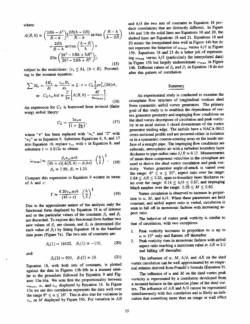
where:

(2Rh- h2' ?R(h- 2R) R-h

2Rh

(2h'-6Rh+SR ),R \ Tp - Tyfi -fi / j,

(15)subject to the restrictions: (to < h), (h < R). Proceed-

ing to the moment equation:

6/-/_ vez H_ 1,-, = L .t = CL pvL(2h)a,

(16)

An expressionfor CL isborrowed from inviscid(finite

wing) airfoiltheory:

2_xo_ (17)- (1+ '

where "x" has been replaced with "_t" and "2" with

"_2" as in Equation 9. Substitute Equations 6, 9, and 17

into Equation 16, replace vc_ with v in Equation 8, andsubstitute t = 0.012c to obtain:

/3oVezo_ch

Iwmax] _ (4h + c)(A(R, h) -/31hc)

/30 = 7.89, /31 = 1.51.

1

"(h) v' (18)

Compare this expression to Equation 9 written in terms

of h and c:

6.20v_oech (h) _F_-, (4h+c) " " (19)

Due to the approximate nature of the analysis only the

functional form displayed by Equation 18 is of interest

and so the particular values of the constants /30 and/31are discarded. To explore this functional form further two

new values of/31 are chosen, and/30 is determined (for

each value of 131) by fitting Equation 18 to the baseline

data point (Figure 7a). The two sets of constants are:

to(l) = 16422, fl1(1) = -110, (20)

and:

/3o(2) = 920, /31(2) = 10. (21)

Equation 18, with both sets of constants, is plotted

against the data in Figures 13b-16b in a manner simi-lar to the procedure followed for Equation 9 and Fig-

ures 13a-16a- We note first the proportionality between

w,_,_, a, and re= displayed by Equation 18. In Figure13a we see this correlation represents the data well over

the range 8 ° < a < 16% This is also true for variation inv_= or M displayed by Figure 16b. For variation in AR

and h/6 the two sets of constants in Equation 18 pro-duce correlations that are distinctly different. In Figure

14b and 15b the solid lines are Equations 18 and 20, the

dashed lines are Equations 18 and 21. Equations 18 and

20 mimic the interpolated data well in Figure 14b but do

not represent the behavior of wm_ versus hi6 in Figure

15b. Equations 18 and 21 do a better job of represent-

ing wmax versus hi6 (particularly the interpolated data)

in Figure 15b but largely underestimate Wrnax in Figure14b. Different values of/30 and/_1 in Equation 18 do not

alter this pattern of correlation.

Summary

An experimental study is conducted to examine the

crossplane flow structure of longitudinal vortices shed

from symmetric airfoil vortex generators. The primary

goal of this study is to establish the dependence of vor-

tex generator geometry and impinging flow conditions onthe shed vortex descriptors of circulation and peak vortic-

ity at an axial station 1 chord downstream of the vortexgenerator trailing edge. The airfoils have a NACA 0012

cross-sectional profile and are mounted either in isolation

or in a symmetric counter-rotating army on the inside sur-

face of a straight pipe. The impinging flow conditions aresubsonic, atmospheric air with a turbulent boundary layer

thickness to pipe radius ratio 6/R ,_ 0.17. Measurements

of mean three-component velocities in the crossplane areused to derive the shed vortex circulation and peak vor-

ticity. Vortex generator angle-of-attack is varied overthe range: 8* < a _< 20', aspect ratio over the range:

0.64 < AR < 2.55, span-to-boundary layer thickness ra-

tio over the range: 0.14 < h/6 < 0.57, and impingingMach number over the range: 0.25 < M < 0.60.

Vortex circulation is observed to increase in propor-

tion to a, M, and h/6. When these parameters are heldconstant, and airfoil aspect ratio is varied, circulation isseen to fall off in monotonic fashion with increasing as-

pect ratio.

The behavior of vortex peak vorficity is similar to

that of circulation, with two exceptions:

1. Peak vorticity increases in proportion to a up toa _, 16 ° only and flattens off thereafter.

2. Peak vorticity rises in monotonic fashion with airfoil

aspect ratio reaching a maximum value at AR ,,_ 2.0

and falling off thereafter.

The influence of _, M, h/6, and AR on the shed

vortex circulation can he well approximated by an empir-

ical relation derived from Prandtl's formula (Equation 9).

The influence of _ and M on the shed vortex peak

vorticity is represented by a correlation developed froma moment-balance in the spanwise plane of the shed vor-

tex. The influence of AR and h/6 cannot be represented

simultaneously with this correlation and is likely an indi-

cation that something more than an image or wall effect

15

is responsible for the behavior of peak vorticity versus

AR and h/,L

Acknowledgements

This project was supported with funding from NASALewis and the National Research Council. The authors

would like to acknowledge the skillful support provided

by many. Appreciated were the mechanical skills of

William Darby and Bob Ehrbar (from NASA's Test In-

stallation Division) and the systems engineering support

of Robert Gronski (NYMA). Charles Wasserbauer (also

of NYMA) provided engineering and operational sup-

port. Design engineering service was provided by Arthur

Sprungle of NASA Lewis. Dr. Warren R. Hingst pro-vided valuable insight into the test section design and

Bernie Anderson aided this effort with his computations

of vortex generator flowfields and his enthusiasm for the

subject. Jeffry Foster (Iowa State graduate assistant)

helped in acquiring the data. Finally, a special thank

you to Mr. T. Nugent who kept our collective noses to

the grindstone throughout the long course of this project.

References

1Reichert, B. A. and Wendt, B. J., "Improving Diffusing

S-Duct Performance by Secondary Flow Control," AIAA

Paper 94-0365, Jan. 1994.

2Foster, J., Okiishi, T. H., Wendt, B. J., and Re-

ichert, B. A., "Study of Compressible Flow Through a

Rectangular*to-Semiannular Transition Duct," NASA CR4660, Apr. 1995.

3Anderson, B. H. and Farokhi, S., "A Study of Three

Dimensional Turbulent Boundary Layer Separation and

Vortex Flow Control Using the Reduced Navier-StokesEquations," Turbulent Shear Flow Symposium tech. rep.,1991.

4 Anderson, B. H. and Gibb, J., "Application of Com-

putational Fluid Dynamics to the Study of Vortex Flow

Control for the Management of Inlet Distortion," AIAA

Paper 92-3177, July 1992.

5Cho, S. Y. and Greber, I., Three Dimensional Compress-

ible Turbulent Flow Computations for a Diffusing S-DuctWith/Without Vortex Generators, Ph.D. Dissertation, Case

Western Reserve University, Cleveland, OH, Nov. 1992.

6Wendt, B. J., Reichert, B. A., and Foster, J. D., "The

Decay of Longitudinal Vortices Shed from Airfoil Vortex

Generators," AIAA Paper 95-1797, June 1995.

7Westphal, R. V., Pauley, W. R., and Eaton, J. K.,

"Interaction Between a Vortex and a Turbulent Boundary

Layer-Part l: Mean Flow Evolution and TurbulenceProperties," NASA TM 88361, Jan. 1987.

s Wondt, B. J. and Hingst, W. R., "Flow Structure in the

Wake of a Wishbone Vortex Generator," A/AA Journal,

Vol. 32, Nov. 1994, pp. 2234-2240.

9Pauley, W. R. and Eaton, J. K., "The Fluid Dynamicsand Heat Transfer Effects of Streamwise Vortices Embed-

ded in a Turbulent Boundary Layer," Stanford University

Tech. Rep. MD-51, Stanford, CA, Aug. 1988.

l°Wendt, B. J., Grebe,, I., and Hingst, W. R., "The

Structure and Developmem of Streamwise Vortex Arrays

Embedded in a Turbulent Boundary Layer," AIAA Paper92-0551, Jan. 1992.

11Porro, A. R., I-fingst, W. R., Wasserbauer, C. A., and

Andrews, T. B., "The NASA Lewis Research Center

Internal Fluid Mechanics Facility," NASA TM 105187,Sept. 1991.

12Zilliac, G. G., "Modelling, Calibration, and Error

Analysis of Seven-Hole Probes," Experiments in Fluids,Vol. 14, 1993, pp. 104-120.

13Moffat, R. J., "Contributions to the Theory of Single-

Sample Uncertainty Analysis," Transactions of the ASME,

Vol. 104, June 1982, pp. 250-258.

I,t Abbott, I. H. and Doenhoff, A. E. V., Theory of WingSections, 2nd eeL, Dover, New York, 1959.

t5 Prandtl, L., "Applications of Modern Hydrodynamics

to Aeronautics," NACA Report 116, 1921.

16

Form ApprovedREPORT DOCUMENTATION PAGE OMBNo. 0704-0188

Public _ bunhm let ttm miKtlon ol _ommlm is emlmated to avlra_ 1 hourper r_;mme. Inctud_ me tlnw t(x m,m,a¢_ Imuuc#em. mamNng mtm_i area eeumm.ga_ng and maimalnt_ the dam needed, w_l _ aml mqmtng the coUe¢eonof Intmmsim. bad mmmmts mgarei_ em be=lee raceme e¢ any oew mpect of mb_,m_ ¢ tr,t_mee. ]ed,x_ .,mmeom_ rm.ee¢,_ buret3tow_oe _ Sen,t:_.a--aone*_ _ _ _ _ 12_5_Oavtz Highwe/, Suae 1204, _ VA 22202-4.102, and to me OIf_ _ Manaeemmt and Bu<ll_. Papemork ReductionPreVpd(0704-01U), WaeV_ltm_ IX: 2O6O3.

1. AGENCY USE ONLY (LeavebianlO 2. REPORT DATE

June 1996

4. TITLE AND SUBTITLE

The Modelling of Symmetric Airfoil Vortex Generators

e. AUTHOR(S)

BJ. Wendt and B.A. Reichert

7. PERFORMING ORGANIZATION NAME(S) AND ADDRESS(ES)

Modem TechnologiesCorporation

Cleveland Office

7530 Lucerne Drive

Islander Two, Suite 206

Middleburg Heights, Ohio 441309. SPONSORING/MONITORINGAGENCYNAME(S)ANDADDRESS(B)

National Aeronautics and Space AdminiswationLewis Research Center

Cleveland, Ohio 44135-3191

3. REPORT TYPE AND DATES COVERED

Final Conuactor Report

S. FUNDING NUMBERS

WU-505-62-52

C-NAS3-27377

8. PERFORgENG ORGANIZATION

REPORT NUMBER

E-10315

10. SPONSORING/MONITORINGAGENCY REPORT NUMBER

NASA CR-198501

AIAA-96-0807

11. SUPPLEMENTARY NOTES

Prepared for the 34th Aerospace Sciences Meeting end Exhibit, Reno, Nevada, Jamua'y 15--18, 1996. BJ. Wendt, Modem TeclmologiesCorporation, Middleburg Heights, Ohio 44130 and B.A. Reichert, Kansas State University, Manhamm, Kansas 66506. Project Manager,John M. Abbott, NASA Lewis Research Center, Internal Fluid Mechanics Division, organization code 2660, (216) 433-3607.

12a. DISTRIBUrTIOFgAVAILABiLITY STATEMENT

Unclassified-Unlimited

Subject Category 02

This publication is available fzom the NASA Center for AexoSpace Infmmaficn, (301) 621---0390.

121. DISTRIBUTION CODE

_3. ABSTRACT(Magnum 200 words)

An experimental study is conducted to determine the dependence of vortex generator geometry and impinging flow

conditions on shed vortex circulation and crossplane peak vorticity for one type of vortex generator. The vortex generator

is a symmetric airfoil having a NACA 0012 cross-sectional profile. The geometry and flow parameters varied include

angle-of-attack u., chordlength c, span h, and Mach number M. The vortex generators are mounted either in isolation or in

a symmetric counter-rotating array configuration on the inside surface of a slraight pipe. The tm'bulent boundary layer

thickness to pipe radius ratio is _¢R = 0.17. Circulation and peak vorticity data are derived from crossplane velocity

meastwements conducted at or about I chord downslream of the vortex generator trailing edge. Shed vortex circulation is

observed to be proportional to M, a, and MS. grzth these parameters held constant, circnlafion is observed to fall off in

monotonic fashion with increasing airfoil aspect ratio AR. Shed vortex peak vorticity is also observed to be propocdonal toM, a, and h/8. Unlike circulation, however, peak vorticity is observed to increase with increasing aspect ratio, reaching a

peak value at AR = 2.0 before falling off.

14. SUBJECT TERMS

Vortices; Vortex genemtQts; Three-dimensional boundary layer

17. SECURITY CLASSIRCATIONOF REPORT

Unclassified

NSN 7540-01-280-5500

18. SECURITY CLASSIFICATION

OF THIS PAGE

Unclassified

19. SECURITY CLASSIFICATION

OF ABSTRACT

Unclassified

15. NUMBER OF PAGES

]816. PRICE CODE

A03

20. LIMITATION OF ABSTRACT

Standard Form 298 (Rev. 2-89)

Prescribed by ANSI S_d. Z39-18298-102

_-- < o|. _ _._'_ o_..o

_ o_ -'o

_:_ _-_I ,°1 .. m

Z _

"in

[.-

3