An Efficient Monte-Carlo Algorithm

for

The Type II Maximum Likelihood Approach

to

Parameter Estimation of Non-linear Diffusions

Yuan Shen1, D. Cornford1, C. Archambeau2, and M. Opper3

1. Neural Computing Research Group, Aston University;

2. Department of Computer Science, University College London;

3. Artificial Intelligence Group, Technical University Berlin.

1

Outline

• The Mathematical Setting of Bayesian inference in nonlinear

diffusions

1. Full Bayesian Treatment

2. Type II Maximum Likelihood

• Monte Carlo Maximum Likelihood Methods

1. Bennett’s Acceptance Ratio Method

2. Wang-Landau’s Random-Walk Algorithm

• Numerical Experiments

1. The Log Marginal Likelihood Profiles

2. The Asymptotic Behaviour of Parameter Estimation

• Future Work

2

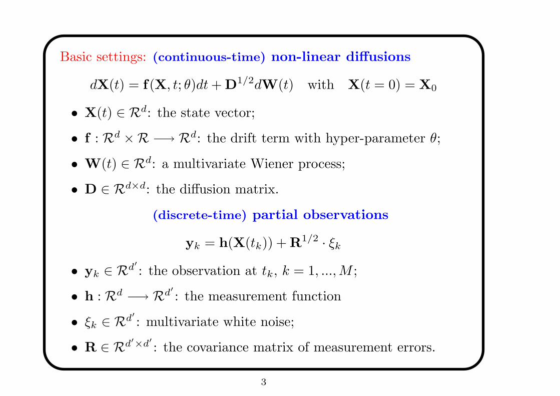
Basic settings: (continuous-time) non-linear diffusions

dX(t) = f(X, t; θ)dt + D1/2dW(t) with X(t = 0) = X0

• X(t) ∈ Rd: the state vector;

• f : Rd ×R −→ Rd: the drift term with hyper-parameter θ;

• W(t) ∈ Rd: a multivariate Wiener process;

• D ∈ Rd×d: the diffusion matrix.

Basic settings: (discrete-time) partial observations

yk = h(X(tk)) + R1/2 · ξk

• yk ∈ Rd′

: the observation at tk, k = 1, ..., M ;

• h : Rd −→ Rd′

: the measurement function

• ξk ∈ Rd′

: multivariate white noise;

• R ∈ Rd′×d′

: the covariance matrix of measurement errors.

3

Toy Example: Stochastic Double-Well Systems

dx = 4x(1 − x2)dt + κdw

0 50 100 150 200 250 300 350 400 450 500−1.5

−1

−0.5

0

0.5

1

1.5κ = 0.5

t

x

0 50 100 150 200 250 300 350 400 450 500−2

−1

0

1

2

t

x

κ = 1.0

4

A Full Bayesian Treatment

p(X(t),D|{y1, ...,yM}) ∝ p(D) · p(X0) · exp(−Hdyn)︸ ︷︷ ︸

p(X|D)︸ ︷︷ ︸

p(X,D)

· exp(−Hobs)︸ ︷︷ ︸

p(Y|X)

0 = t1 < t2, ... < tM−1 < tM = T

Hdyn =1

2

∫ T

0

∣∣∣∣

∣∣∣∣

dX

dt− f(X, t)

∣∣∣∣

∣∣∣∣

2

D︸ ︷︷ ︸

Onsager-Machlup

Hobs =1

2

M∑

k=1

||yk − h(X(tk))||2R

||a||2A = a>A−1a

−→ Markov Chain Monte Carlo (MCMC)

5

MCMC estimation of state X (Hybrid Monte Carlo)

0 5 10 15 20 25 30 35 40 45 50−2.0

−1.5

−1.0

−0.5

0.0

0.5

1.0

1.5

2.0

Time t

Stat

e x

Joint estimation of X and D (Gibbs sampling) −→ slow

convergence due to high dependence between X- and D samples

6

Type II Maximum Likelihood Method

The posterior of X

p(X|Y,D) =p(Y|X) · p(X|D)

∫

dX · p(Y|X) · p(X|D)

︸ ︷︷ ︸

p(Y|D)

−→ Marginal likelihood p(Y|D)

Type II Maximum Likelihood Estimate of D and X

D̂ = maxD p(Y|D)

p(X|D̂,Y) ∝ p(Y|X) · p(X|D̂)

−→ Monte Carlo Maximum Likelihood

−→ Problems: Difficulties in calculating the ratio of

normalising constants p(Y|D1) : p(Y|D2) : p(Y|D3) : ....

7

Bennett’s Acceptance Ratio Method

• Two posterior densities p1 = p(X|D1,Y) and p2 = p(X|D2,Y)

with their normalising constants Z1 and Z2, respectively −→

compute Z1

Z2

by Metropolis-Hastings;

• Running a Metropolis-Hastings algorithm with a transition

kernel T (·|·) that allows moves between π1 = p(X|D1,Y) · ω1

and π2 = p(X|D2,Y) · ω2 where ω1 and ω2 are so-called

pseudo-prior for index I in an extended state space [X, I] (see

simulated tempering literature);

• The ratio of normalising constants Z1

Z2

= ω1

ω2

−→ The uniform

distribution of occupation numbers P(I=1)P(I=2) = 1

[Z1

Z2

]

·ω2

ω1=

Z1/ω1

Z2/ω2=

Ep1[T (π2|π1)]

Ep2[T (π1|π2)]

=α(π1 → π2)

α(π2 → π1)=

P(I = 1)

P(I = 2)

8

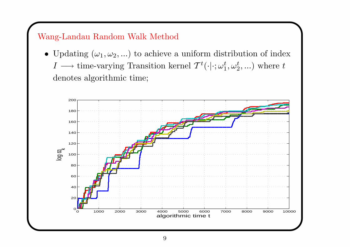
Wang-Landau Random Walk Method

• Updating (ω1, ω2, ...) to achieve a uniform distribution of index

I −→ time-varying Transition kernel T t(·|·; ωt1, ω

t2, ...) where t

denotes algorithmic time;

0 1000 2000 3000 4000 5000 6000 7000 8000 9000 100000

20

40

60

80

100

120

140

160

180

200

algorithmic time t

log ω k

9

• Define a schedule ωtk,

ωtk = ωt−1

k · (1 + γt−1 · δkIt−1)

where γt is an external, deterministic scalar process of positive

and non-increasing values −→ a controlled Markov chain;

0 2 4 6 8 10 12

x 104

0

0.1

0.2

0.3

0.4

0.5

0.6

0.7

0.8

0.9

1

algorithmic time t

γt

10

• An example of the process γ:

γt = (1 + γ0)1

2j − 1 ∀t ∈ [τj−1, τj ].

where {τj} are random times (except for τ0 = 0);

• The choice of random times {τj}

1. t = τj : Htk = 0 and t > τj : Ht+1

k = Htk + δkIt ;

2. If Ht is sufficiently flat, then set τj+1 = t.

0 2 4 6 8 10 12 14 16 18 200

0.05

0.1

0.15

0.2

0.25

0.3

0.35

0.4

0.45

0.5

index I

histogr

am H

11

Numerical Experiments

• Toy example

dx = 4x(1 − x2)dt + κdw with κ = 1.0

• Comparison of log marginal likelihood profiles

– Investigation of asymptotic behaviour 1: observation

window size T −→ ∞ (fixed M)

– Investigation of asymptotic behaviour 2: observation

density M per time unit −→ ∞ (fixed T )

12

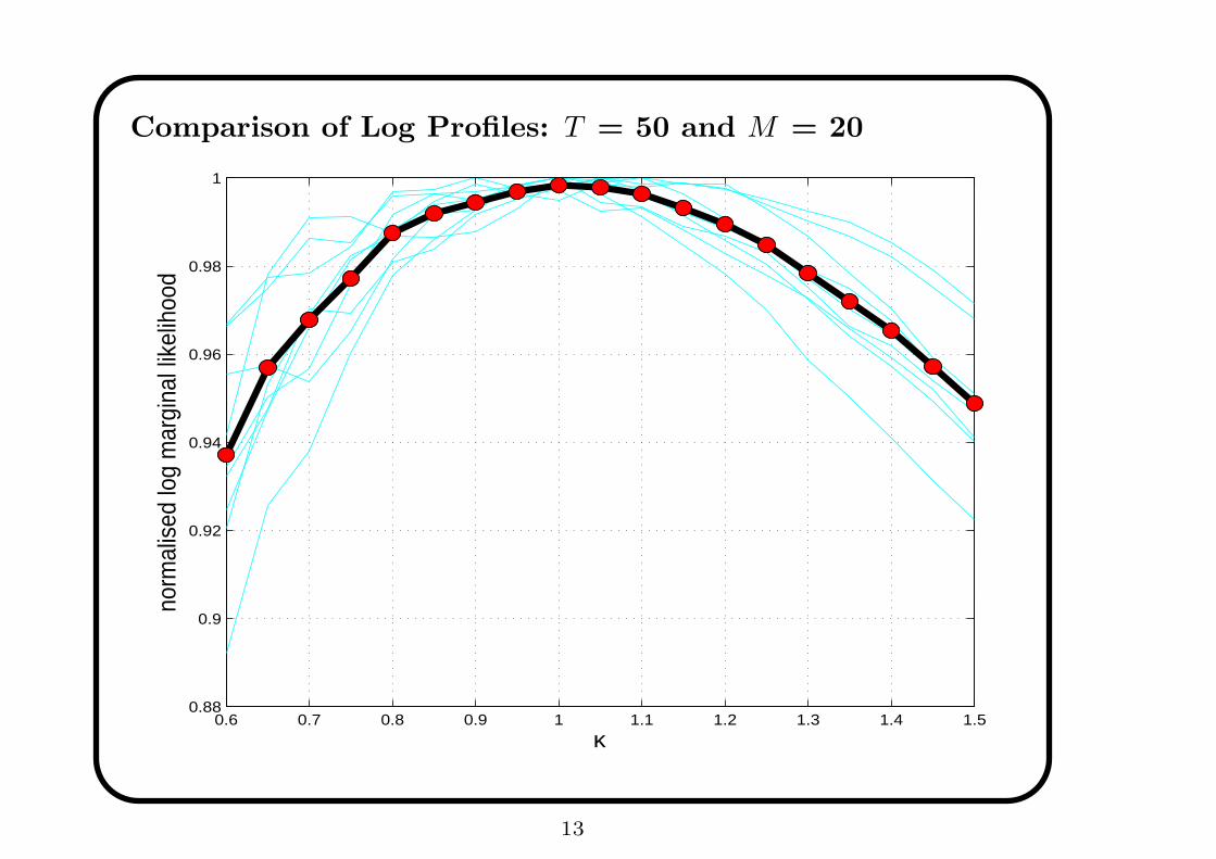
Comparison of Log Profiles: T = 50 and M = 20

0.6 0.7 0.8 0.9 1 1.1 1.2 1.3 1.4 1.50.88

0.9

0.92

0.94

0.96

0.98

1

κ

norm

alis

ed lo

g m

argi

nal l

ikel

ihoo

d

13

Comparison of Log Profiles: T = 50 and M = 1

0.6 0.7 0.8 0.9 1 1.1 1.2 1.3 1.4 1.50.92

0.93

0.94

0.95

0.96

0.97

0.98

0.99

1

κ

norm

alis

ed lo

g m

argi

nal l

ikel

ihoo

d

14

0 10 20 30 40 50−2

−1.5

−1

−0.5

0

0.5

1

1.5

2

0 10 20 30 40 50−2

−1.5

−1

−0.5

0

0.5

1

1.5

2

0.5 0.6 0.7 0.8 0.9 10

100

200

300

400

500

600

700

800

900

1000

κ

exit tim

e

1 1.1 1.2 1.3 1.4 1.50

1

2

3

4

5

6

7

8

9

10

κ

exit tim

e

15

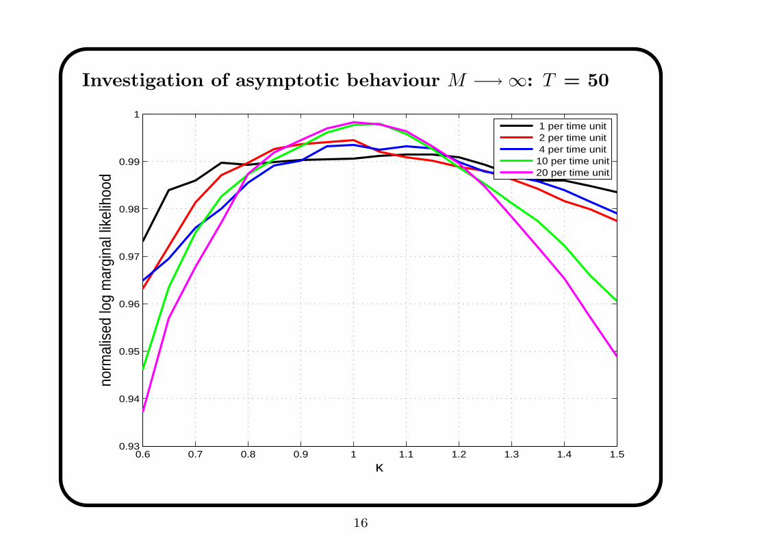
Investigation of asymptotic behaviour M −→ ∞: T = 50

0.6 0.7 0.8 0.9 1 1.1 1.2 1.3 1.4 1.50.93

0.94

0.95

0.96

0.97

0.98

0.99

1

κ

norm

alis

ed lo

g m

argi

nal l

ikel

ihoo

d

1 per time unit 2 per time unit 4 per time unit10 per time unit20 per time unit

16

Investigation of asymptotic behaviour T −→ ∞: M = 4

0.6 0.7 0.8 0.9 1 1.1 1.2 1.3 1.4 1.50.96

0.965

0.97

0.975

0.98

0.985

0.99

0.995

1

1.005

κ

norm

alis

ed lo

g m

argi

nal l

ikel

ihoo

d

t = 5t = 10t = 20t = 30t = 40t = 50

17

Investigation of asymptotic behaviour T −→ ∞: M = 20

0.6 0.7 0.8 0.9 1 1.1 1.2 1.3 1.4 1.50.93

0.94

0.95

0.96

0.97

0.98

0.99

1

κ

norm

alis

ed lo

g m

argi

nal l

ikel

ihoo

d

t = 5t = 10t = 20t = 30t = 40t = 50

18

Variational Approximation Method

• Q(X|D): a Gaussian approximation to the posterior measure

P(X|Y,D);

• Variational Free Energy

F(D) = − lnP(Y|D) + KL(Q̂(X|D)||P(X|Y,D))

where

Q̂(X|D) = minQ KL(Q(X|D)||P(X|Y,D))

• The variational estimate of D

D̂ = minD F(D)

• Profile Comparison:

F(D) ≥ − lnP(Y|D)

19

Future work

• Comparison of log profiles and point estimates (Type 2

Maximum Likelihood)

• Comparison of posterior distribution (Full Bayesian Treatment)

• Wang-Landau Monte-Carlo Maximum-Likelihood

for the joint estimation of drift- and diffusion parameter;

• Variational MCMC for parameter estimation.

20