TI 2006-047/3 Tinbergen Institute Discussion Paper

An Almost Integration-free Approach to Ordered Response Models

Bernard M.S. van Praag* Ada Ferrer-i-Carbonell**

SCHOLAR, Faculty of Economics and Econometrics, University of Amsterdam, and Tinbergen Institute. * CESifo, and IZA. ** AIAS Amsterdam Institute of Labour Studies.

Tinbergen Institute The Tinbergen Institute is the institute for economic research of the Erasmus Universiteit Rotterdam, Universiteit van Amsterdam, and Vrije Universiteit Amsterdam. Tinbergen Institute Amsterdam Roetersstraat 31 1018 WB Amsterdam The Netherlands Tel.: +31(0)20 551 3500 Fax: +31(0)20 551 3555 Tinbergen Institute Rotterdam Burg. Oudlaan 50 3062 PA Rotterdam The Netherlands Tel.: +31(0)10 408 8900 Fax: +31(0)10 408 9031 Please send questions and/or remarks of non-scientific nature to driessen@tinbergen.nl. Most TI discussion papers can be downloaded at http://www.tinbergen.nl.

1

An Almost Integration-free Approach to Ordered Response

Models

Bernard M.S. Van Praag*

Tinbergen Institute, CESifo, IZA, & SCHOLAR, Faculty of Economics and Econometrics

University of Amsterdam

and

Ada Ferrer-i-Carbonell

SCHOLAR, AIAS Amsterdam Institute of Labour Studies, & Tinbergen Institute

Faculty of Economics and Econometrics University of Amsterdam

Amsterdam, 19 April 2006

Acknowledgments: We are very grateful for the comments by J.S.Cramer and A.

Kapteyn on earlier versions. The responsibility for this paper lies with the authors.

* Correspondence author: Faculty of Economics and Econometrics, SCHOLAR, University of Amsterdam. Roetersstraat 11; 1018 WB Amsterdam; the Netherlands. E-mail: B.M.S.vanPraag@uva.nl

2

An Almost Integration-free Approach to Ordered Response

Models

Abstract In this paper we propose an alternative approach to the estimation of ordered response

models. We show that the Probit-method may be replaced by a simple OLS-approach,

called P(robit)OLS, without any loss of efficiency. This method can be generalized to the

analysis of panel data. For large-scale examples with random fixed effects we found that

computing time was reduced from 90 minutes to less than one minute. Conceptually, the

method removes the gap between traditional multivariate models and discrete variable

models

JEL-Codes: C25.

Keywords: Categorical data; Ordered probit model; Ordered response models;

Subjective data; Subjective well-being.

3

1. Introduction.

The main task of econometric methodology is to estimate relationships between variables

y and variables x. The oldest example is OLS, where we try to explain a variable y by a

linear combination of variables x. The expected structural relation is then 0y xβ β′≈ + ,

which we make exact by adding an error term, viz., 0y xβ β ε′= + + . It is assumed that

the random vector of explanatory variables and the random residual are mutually

independent1. The unknown β 's are estimated by minimizing the sum of squared

residuals. Mostly this procedure is defended on the basis of probabilistic assumptions

under which the OLS- procedure is identical with maximum- likelihood estimation. There

is now a well-established family of methods, like simultaneous equations, principal

components, etc., in short the body of literature, which is called the 'linear model' or

'multivariate statistics', that may be seen as generalizations of the OLS- model.

There are however situations where we have difficulty with applying such models. It may

be that the variable to be explained is ordinally continuous. We think of preference

orderings where situations, conditions or commodity bundles x are ordered according to a

preference ordering ≺ . Under rather general conditions such a preference ordering may

be described by a utility function ( )U x , such that (1) (2)x x≺ if and only if

(1) (2)( ) ( )U x U x< . We know, following Pareto (1906) and Debreu (1959), that in such a

case only the indifference curves, described by equations ' ( ) constantU x = ', are

determined and observable, but that the function U(.) as such has no cardinal

interpretation. It is just a labeling system, that may be replaced by any function

1 In the literature one chooses often the slightly more general assumption that the explanatory variables and the residual are uncorrelated. We prefer the independence assumption as being more intuitive.

4

(.) ( (.))U Uϕ= , where ϕ (.) is a monotonically increasing function on the range of U(.).

The situation may be even more complicated if the preference ordering is only discretely

observed, e.g., in terms of verbal categories like 'bad', 'sufficient', 'good' or numerical

categories 1,2,…7, where no cardinal meaning can be assigned to the numerical values.

Then we have ordered response sets 1 2 ....A A≺ ≺ . Such problems are mostly approached

by using an Ordered Probit (OP) or an Ordered Logit -model.

The Ordered Probit (OP) and Ordered Logit (OL) models belong to the main traditional

statistical workhorses in applied econometric studies. They are applied to cases where the

range of possible events can be ordered or ranked in terms of more or less preferred,

higher or lower, better or worse, more or less probable, more or less propensity to be

employed. These are ordered response models. The model is implemented by the

introduction of a latent variable ( , ; )Y f X Xε β β ε′= = + , where the function f(.) is

mostly taken to be linear after suitable transformation of the variables involved. Then we

postulate that the chance on the observation of iA is ( ) ( )i iP A P Y A= ∈ , where we assume

that the intervals 1( , ]i i iA μ μ−= constitute a partition of disjoint intervals on the real axis.

Maximization of the log-likelihood with respect to the 'nuisance parameters' μi and the

parameters β yields the estimates. This is the usual approach when we deal with

'satisfactions' or 'propensities'. Those 'satisfactions' or 'propensities' may deal with how

satisfied individuals are with their life, with their income, or with a specific opera

performance in terms of verbal descriptions, ranging from 'terrible' to 'delighted'. The

same holds for individuals that we may order in, e.g., being less or more likely to be

employed. Such variables are frequently encountered in economics and especially in the

5

now flourishing subjective satisfaction literature2. Beyond economics ordered- response

models are used in many other fields like psychology, sociology, political science,

medicine and biology. We refer for still relevant surveys to Amemiya (1981) and

Maddala (1983). More recent surveys are by Dhrymes (1986), Long (1997), DeMaris

(2004), and Greene (2005). The ordered response models entail computational problems.

However, in modern software packages (e.g. STATA, LIMDEP) the problems involved

in the estimation of a single equation (Probit, Logit) have been sufficiently tackled.

Nevertheless, when we try to apply ordered response models on more general models

than the simple OLS-equation we easily run into difficulties. For instance, when we like

to apply the method in panel analysis where we want to take into account the panel

structure either by assuming that the error terms between different observations of the

same individual are correlated (individual random effects) or by introducing individual

fixed effects (see Greene, 2005), many computational problems appear, when the one-

dimensional integrals have to be replaced by multi-dimensional integrals, where

integration problems tend to become overwhelming. Another example is the estimation of

a system of equations. Although the conceptual model is just the traditional linear model,

there arise problems when we like to extend the usual econometric toolkit, if latent

variables are involved. Our method is much easier to implement, as it does not require

many integrations. To be more precise, if the number of distinct response categories is k,

we need (k-1) normal integrations, in most practical cases a number smaller than 10. In

the traditional OP- approach we need N integrals, one per observation n. If we take into

2 See, e.g., Clark and Oswald, 1994; DiTella et al., 2001; Easterlin, 2001; Ferrer-i-Carbonell, 2005; Ferrer-i-Carbonell and Frijters, 2004; Frey and Stutzer, 2002; Blanchflower and.Oswald, 2004; Frijters, Haisken-DeNew, and Shields, 2004; van Praag, 1971;Van Praag and Ferrer-i-Carbonell, 2004; and Van Praag, Frijters, and Ferrer-i-Carbonell, 2003.

6

account that Probit-estimation is typically solved by means of a few iteration rounds, say

5, then the number of integrations is 5N. So, if we have 10 response categories and 2000

observations, the traditional approach requires 10,000 integral computations, why for our

method 9 integrals are sufficient. In our empirical results in Section 6 we will see that this

will give a tremendous reduction of computer time. In a rather realistic model of a

random fixed effect panel model the traditional approach requires about one and a half

hour, while the same estimation by our method requires about a minute.

When we consider the situation we feel that the ordered response literature is much more

built up from solutions to isolated problems than the general linear model literature and

that therefore it stands somewhat apart as a different field from mainstream statistics and

econometrics.

In this paper we will try to bridge that gap by proposing a specific OLS –approach that

avoids the integration problems. In section 2 we shall have a close look at OP and its

relationship with OLS. In section 3 we introduce an alternative to Probit, which we will

call the Probit OLS (POLS)- method. In Section 4 we compare the POLS –approach with

Ordered Probit. Our conclusion is that they are equivalent. In Section 5 we compare the

POLS –approach with Ordered Probit on the basis of an empirical data set. The empirical

findings confirm the equivalence of both methods. In Section 6 we apply the method to a

panel data set with individual random effects. In Section 7 we compare the POLS-method

with the Linear Probability method in the specific case of a binary response variable. It is

easily seen that much of what we do lends itself for a Logit-type treatment as well; we

consider and evaluate this briefly in Section 8. In Section 9 we draw some conclusions.

7

The main conclusion of this paper is that it seems possible to enroll all ordered response

problems within the body of the well-established statistical –econometric toolkit of linear

models. Computationally, it implies a significant reduction of computing time. Therefore,

there would be hardly any need for a separate body of computationally hard methods

dealing with ordered response analysis. For other empirical applications in a panel

context or/and where the latent variables appear 'at the left-hand side' as well, we refer to

Van Praag and Ferrer-i-Carbonell (2004), Van Praag, Frijters, and Ferrer-i-Carbonell

(2003), and Van Praag and Baarsma (2005).

2. The relation between OLS and the Ordered Probit (OP) model.

In this section we will look for the relation between the OLS –estimators and the

corresponding Probit-estimator, if the dependent variable is observed through an ordered

response mechanism. In order to avoid unnecessary abstraction we cast our analysis in

terms of a satisfaction context. It will be obvious that the analysis as such is completely

general.

We consider individual self-reported financial satisfaction3 μ, which is assumed to

depend on log-income (inc) and log-family size (fs) according to the relation

1 2 0. .inc fsβ β β ε μ+ + + = (2.1)

or

X β ε μ′ + = (2.2)

3 For the context see also Van Praag and Ferrer-i-Carbonell, 2004, chapter 2

8

for short. For each value of μ this equation describes an 'equal satisfaction' - or

indifference –line on the (inc,fs,ε ) -space. We assume X and ε to be random and mutually

independent. It follows that μ is a random variable as well. Moreover, we assume ε to be

N (0,1)-distributed.

The trade–off ratio between inc and fs is defined by 2 1/β β . If personal conditions

change by incΔ and fsΔ such that incΔ = ( 2 1/β β− ). fsΔ , the individual stays on the

same indifference curve.

Let us now assume, quite realistically, that it is impossible to distinguish between very

small satisfaction differences.

This implies that the dense net of indifference curves is replaced by a set of just k non-

overlapping ‘indifference strips’ on the (inc, fs)-space (see Figure 1). Each indifference

strip i has a lower and upper boundary, corresponding to the indifference curves labeled

by 1iμ − , and iμ . The curve corresponding to the level iμ is a 'group-average' curve in a

sense to be made precise later on.

Fig. 1. Indifference curves in the (income, family size) – space.

Family Size

Income

μi-1

iμμi

Unhappier

9

Since ε is assumed to be N (0,1)- distributed, the likelihood of observation n, being in

response category ni is

1 1

1

( ) ( )

( ) ( )

i n i i n i n

i n i n

P x P x x

N x N x

μ β ε μ μ β ε μ β

μ β μ β

− −

−

′ ′ ′< + ≤ = − < + ≤ −

′ ′− − − (2.3)

where N(.) stands for the standard- normal distribution function.

Applying the ML-estimation principle we differentiate the logarithm of (2.2) with respect

to β yielding

1

1

( ) ( )ln( ) .( )( ) ( )

i n i nn

i n i n

n x n xP xN x N x

μ β μ ββ μ β μ β

−

−

′ ′− − −∂= −

′ ′∂ − − − (2.4)

Now we have (see, e.g., Johnson and Kotz, p.81, 1970 and Maddala, p.366, 1983) for the

conditional expectation of the normal distribution the general formula

( ) ( )

( ; , ) .( ) ( )

A m B mn ns sE X m s A X B m sB m A mN Ns s

− −−

< ≤ = +− −

− (2.5)

where X is N(m,s)-distributed.

Using this formula we may rewrite (2.4) as

10

1 ,ln( ) ( ;0,1 ).( )n

i n i n n jj

P E x x xε μ β ε μ ββ −

∂ ′ ′= − < ≤ − −∂

(2.6)

or

1 ,

1 ,

ln( ) ( ;0,1 ).( )

[ ( ;0,1 )].( )

i i n jj

n i i n j

P E x

E x x

ε μ μ μβ

μ β μ μ μ

−

−

∂= < ≤ −

∂

′= − < ≤ −

(2.7)

If we sum over the observations we get the normal equation system

1 ,1 1

ln( ) [ ( ;0,1 ) ].( ) 0n n

N Nn

i i n n jn nj

P E x xμ μ μ μ ββ −

= =

∂ ′= < ≤ − − =∂∑ ∑ (2.8)

We see that this is just the familiar orthogonality condition of regression analysis, where

the variable μ is replaced by its conditional expectation 1( ;0,1 )n n

def

i i iE μ μ μ μ μ− < ≤ = ,

yielding the system

( )X X Xβ μ′ ′= (2.9)

This is equivalent to regressing μ on X instead of μ itself. The difference

,( )def

i i withinμ μ ε− = may be seen as a measurement error with respect to the variable μ to be

explained. Its expectation is zero and its total variance is 2withinσ . The regression equation

becomes

11

withinXμ β ε ε′= + − (2.10)

yielding a consistent estimator of β. However, compared to the case of continuous

observation where μ itself would be observable this estimator has a greater standard

deviation caused by the increased residual variation.

Consider now the background - model

n n nXμ β ε′= + (2.11)

where β is assumed to be known. It implies a labeling system for the indifference curves.

When nε ε= the observation n lies on the indifference curve n n nXμ β ε′= + .

If X is a random vector with expectation X and variance –covariance matrix XXΣ , it

follows that we know the distribution of the indifference curve labels μ , if we know the

distribution of X and ε. We have ( )E Xμ β ′= and var( ) 1XXμ β β′= Σ + . In view of the

fact that the distance between indifference curves is defined by using the likelihood

2

1

1 ( )2i n

i

xe d

μ μ β

μμ

−

′− −

∫ , where the distance 2( )xnμ β ′− appears in the exponent, the resulting

labeling system may in fact be interpreted as a cardinalization.

If we stick to the ordinal approach to utility and satisfaction, our only information refers

to the shape of the indifference curves. The information on β , or rather on the slope

described by the trade-off ratios, is the same, irrespective of the specific labeling system

used. We will come back to this later.

12

3.The Probit OLS (POLS) - approach.

The regression approach to Probit, as outlined in equations (2.8)-(2.10), is unfeasible in

practice as we do not know the distribution of μ. Consequently, the conditional

expectation in (2.7) cannot be computed. In the POLS- approach we start from the other

end so to speak. We assume that the labels μ of the indifference curves within a

population are distributed according to a continuous distribution function ( )G μ , that is,

there is no indifference curve with a discrete mass of observations on it. Then ( )G μ is

the fraction of the population that is situated on or at a lower satisfaction level than the

one associated with the indifference curve μ. We repeat that in the ordinal approach there

is no cardinal meaning attached to the values μ. This means that we can replace the

values μ by ( ; )μ ϕ μ ζ= , where the function ϕ is monotonically increasing to preserve

the order and where ζ is a set of ϕ -specific parameters. Notice that if ( ; )xμ μ β= , then

( ( ; ); )xμ ϕ μ β ζ= . This implies that both representations describe the same net of

indifference curves. The distribution function of the distribution of μ is

1( ) ( ( ))H Gμ ϕ μ−= . This shows that the distribution function of the label distribution

depends on the specific labeling system. Inversely, it follows that the label distribution

may be any continuous distribution on the real axis, depending on the appropriate choice

of the re-labeling function ϕ (.).

It follows that there is a specific labeling system, for which the distribution of μ will be

standard normal, i.e., ( ) ( ;0,1)H Nμ μ= . We call this labeling system the normal labeling

system. We drop the tilde from now on.

13

Let us now assume that we observe satisfaction in terms of a few discrete response

categories, for example ranging from 'very dissatisfied' to 'very satisfied'.

The range of labels is partitioned in response categories that represent k adjacent intervals

1( , ]i iμ μ− , such that a response I=i (i=1,…,k) implies that the latent

variable 1( , ]i iμ μ μ−∈ . We define 0 , kμ μ= −∞ = ∞ . The categorical frequencies (i.e. the

frequency of responses found in each k category) are 1,..., kp p . Now, if we start off from

the normal labeling system the variable μ is N(0,1)-distributed in the population.

Moreover, we assume a model where μ may be decomposed into a structural part, say

f(X) and a residual part ε, such that the two components are mutually independent. A

rather deep theorem in probability theory, first proved by H. Cramèr in 1937 (see Feller,

1966, Ch. XV, 8, also Rao, 1973, p.525), states that if μ is normally distributed and if it is

the sum of two mutually independent random variables, say f(X) and a residual part ε,

then those two variables have to be normally distributed as well. It implies that the

structural part ( ) f X will be normally distributed as well. This does not imply that all X-

variables separately have to be normal, for they are not assumed to be mutually

independent. But it does imply that ( ) f X cannot be restricted to a proper subset of the

real axis ( , )−∞ ∞ only.

Given the distribution of μ over the population we may estimate the iμ ’s in a simple

manner by solving the equations

1( ) ( ) ( 1,..., 1)i i ip N N i kμ μ −= − = − (3.1)

14

(see for similar thoughts also Terza (1987), Stewart (1983), and Ronning and Kukuk

(1996)).

These are (k-1) equations in (k-1) unknowns 1 1,..., kμ μ − . Although we do not know the

exact value of individual μ's, we now know at least that it lies within a specific interval.

Notice that this result does not depend on the x-values, not brought into play yet, but only

on the distribution of the response categories, that is, the unconditional distribution of μ.

Let us now assume that we try to explain the variable μ by a linear model

,0

m

n POLS j jn nj

Xμ β ε=

= +∑ (3.2)

where 0 1nX ≡ and 0β the intercept4.

Although nμ cannot be directly observed, we may calculate its conditional expectation

(see (2.5))ni

μ = 1( )i iE μ μ μ μ− < ≤ . As already said, for the normal distribution holds the

formula (see, e.g., Maddala, 1983, p.366)

11

1

( ) ( )( )

( ) ( )n n

n n n

n

i ii i i

in i

n nE

N Nμ μ

μ μ μ μ μμ μ

−−

−

−= < ≤ =

− (3.3)

The variable ni

μ is a discrete random variable with chances 1( ) ( )i i ip N Nμ μ −= − .

Now we take ni

μ as a proxy for nμ . We write nμ 1( )n n ni i iEμ ε μ μ μ−= − < ≤ and we

regress ni

μ on the variables x. We estimate the model

4 We denote random variables by capitals and their values by lower case.

15

, , 10

( )n n n

m

i j POLS j n n i iX Eμ β ε ε μ μ μ−= + − < ≤∑ (3.4)

Notice that (2.10) and (3.4) are identical except for a factor of proportionality.

We have the following variance decomposition. The total variance of the continuous μ is

2 ( ) 1σ μ = by definition. The variable ni

μ we observe is a class mean. Its variance is

2 ( ) 1ni

σ μ < . The difference 21 ( )ni

σ μ− is the information loss by observing the

discretized variable ni

μ instead of the continuous latent variable μ behind it. Hence, we

get the decomposition.

2 2

0(1 ( )) var( ) ( ) 1

n

m

i i in nXσ μ β σ ε− + + =∑ (3.5)

The observed 2R is

2 0

2

0

var( )

var( ) ( )

m

i in

m

i in n

XR

X

β

β σ ε=

+

∑

∑ (3.6)

This is an overestimate of the true R2, which equals

16

2 0

2 2

0

var( )var( )

(1 ( )) var( ) ( )n

m

i in

m

i i in n

XR X

X

ββ

σ μ β σ ε′= =

− + +

∑

∑ (3.7)

Or in words, the larger the information loss due to discretization, the larger apparently the

variance explained. It also implies that the residual variance is under-estimated, and

hence that the standard deviations of the estimators are underestimated as well.

Therefore, the corresponding t-ratios are overestimated. The correction factor Δ is easily

assessed to be

02

1 var( )

( )

m

i in

n

xβ

σ ε

−Δ =

∑ (3.8)

It stands to reason that the POLS-method can be used for non-linear models as well after

suitable transformation.

4. Comparison between POLS and Ordered Probit.

The question is now how traditional Ordered Probit compares with the POLS-approach.

The traditional model in OP is again

,0

m

n in i OP ni

Y X β ε=

′= +∑ (4.1)

17

However, the assumptions of the OP- model differ from those of the POLS- model. In OP

the error term is normal N(0,1), but the structural part ,0

( )m

i OP in n OPX Xβ β′=∑ is not

necessarily normal. That implies that the population distribution of the latent variable Y is

not necessarily normal either. However, in practice there are two reasons why there is at

least a reasonable chance that Y will be approximately normal as well. First, the

distribution of many explanatory variables is frequently nearly normal in the population

under study. Second, in econometric practice variables are frequently transformed prior

to the analysis in such a way that their distribution in the population (unintendedly)

becomes approximately normal. An interesting example is income. Frequently we take

log-income as explanatory variable, which is approximately normally distributed in

populations. It is also possible to transform explanatory variables X on purpose by a one-

one monotonous transformation such that the sample distributions of the transform, say

( )X Xϕ= , are N(0,1)-distributed. Thus, the sum ,j j nXβ∑ is ensured to be normal.

Finally, the Central Limit Theorem is at work. Mostly the number of explanatory

variables is between five and ten, which is too small a number to warrant the claim of

accurate normality of their sum, but in practice the difference is mostly negligible. If that

is true, we see that (2.10) and (3.4) are identical systems except for a factor of

proportionality. And inversely, if we find that the systems are different in more than a

factor of proportionality we may infer that the structural part is not approximately

normally distributed in the population.

Under the Probit assumptions the variance of the unknown error is set equal to one,

2 ( ) 1σ ε = . It follows that the variance of the latent OPY equals

18

2 2 2 2( ) ( ) ( ) 1 ( )OP n OP n OPX Xσ μ σ ε σ β σ β′ ′= + = + . Hence, the variance of the Probit latent

variable is larger than that of the POLSμ in the POLS-approach. If both models describe

the same indifference curves, it follows that the coefficients OPβ and POLSβ must have a

fixed ratio 21 ( )( )

n OPOP

POLS

XH

σ βββ σ μ

′+= = . Let us now assume that ( ) 0OPE Y = . This

implies the identification of the intercept 0, ( )OP n OPE Xβ β′= − .5

The chance on a response i in the Probit- model is

1 1

1

( ) ( )

( ) ( )

i OP i i i

i i

P P x x

N x N x

μ μ μ μ β ε μ β

μ β μ β

− −

−

′ ′< ≤ = − < ≤ −

′ ′= − − − (4.2)

The unknown 'nuisance parameters’ (μ) are found by solving the triangular system

1

2

1 1

2 2 2

1 { ( )}

1 { ( ) ( )}

.......

n OPn A

n OP n OPn A

N x pN

N x N x pN

μ β

μ β μ β

∈

∈

′− =

′ ′− − − =

∑

∑ (4.3)

where iA stands for the set of respondents with response i. Notice now that if ( )n OPX β′ is

(approximately) normal the first sum tends to the marginal distribution function

5 We notice that in Ordered-Probit analysis either 0β or the first nuisance parameter 1μ is set at zero. This procedure is needed for identification and does not imply a loss of generality. We partition if needed

0 1( , )β β β= .

19

21( ;0,1 ( ))n OPN xμ σ β′+ . Similarly, the second term tends to

2 22 1[ ( ;0,1 ( ) ( ;0,1 ( )]n OP n OPN X N Xμ σ β μ σ β′ ′+ − + and so on. This is the system (3.1)

except for a different variance. It follows that the Probit -μ 's are related to the POLS -

μ 's according to the relation 21 ( ).OP n OP POLSXμ σ β μ′= + .

If (2.10) and (3.4) are completely equivalent, except for a factor of proportionality, it

follows that POLS and OP are equivalent. The t- values of both methods are the same, as

the factor 21 ( )n OPXσ β′+ cancels out. Hence, both methods would be equally efficient.

It follows that the observed overestimation in POLS, due to discrete observation, of the t

–values and of 2R holds for Probit as well.

5. Empirical illustration.

We applied the above ideas on the Financial Satisfaction Question, which appears in the

German Socio-Economic Panel (GSOEP, wave 1996) and in many other surveys as well.

This question runs as follows:

How satisfied are you with your household income? …………………….

(Please answer by using the following scale, in which 0 means 'totally unhappy' and 10

means 'totally happy')

We explained the answer to this question by two variables, viz. log(household income)

(lny) and log (family size) (lnfs) according to the equation

20

,1 ,2 ,0ln( ) ln( )ni POLS n POLS n POLS ny fsμ β β β ε= + + + (5.1)

where nε stands for the composite error term in (3.4).

We estimated this equation by POLS and by the traditional OP- method. We present the

estimation results of this equation side by side in Table 1.

Table 1. Estimates of the same relation by OP and POLS6. Data:GSOEP, 1996 Ordered Probit POLS Coeff. t-ratio Coeff. t-ratio Ln(y) 0.487 15.070 0.454 15.230 Ln(fs) -0.189 -5.690 -0.176 -5.680 Constant -3.596 -15.11 N = 5179 Log.Like. -9650 R2 0.0429 Adjust. R2 0.0425 Trade-off-ratio 2 1/β β -0.388 -0.387 The intercept terms are now shown in the table.

As predicted in Section 5, we see that both estimates (Probit and POLS) look rather

similar. The important point is that the trade-off ratio 2 1/β β , that is defining the shape of

the indifference curve, is virtually the same for both cases. The t-ratios are the same as

well. Hence, we conclude that OP and POLS are here equivalent indeed.

It is frequently thought that the number of response categories k is irrelevant for the

estimation. This is however not true. We tried the two regression methods on a

transformed data set, where we had just two response categories ‘low’ and ‘high’

financial satisfaction. The border was laid at such a point that both response classes

contain about half the sample, hence the information loss is maximal. The result is a

dependent variable that takes the value 0 if financial satisfaction is equal to or smaller

6 Similar results are presented in Chapter 2 in Van Praag and Ferrer- i –Carbonell (2004).

21

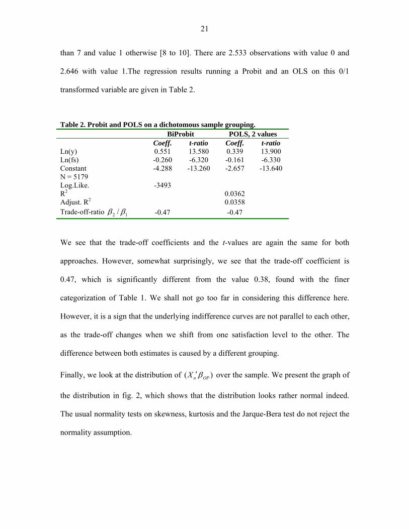
than 7 and value 1 otherwise [8 to 10]. There are 2.533 observations with value 0 and

2.646 with value 1.The regression results running a Probit and an OLS on this 0/1

transformed variable are given in Table 2.

Table 2. Probit and POLS on a dichotomous sample grouping. BiProbit POLS, 2 values Coeff. t-ratio Coeff. t-ratio Ln(y) 0.551 13.580 0.339 13.900 Ln(fs) -0.260 -6.320 -0.161 -6.330 Constant -4.288 -13.260 -2.657 -13.640 N = 5179 Log.Like. -3493 R2 0.0362 Adjust. R2 0.0358 Trade-off-ratio 2 1/β β -0.47 -0.47

We see that the trade-off coefficients and the t-values are again the same for both

approaches. However, somewhat surprisingly, we see that the trade-off coefficient is

0.47, which is significantly different from the value 0.38, found with the finer

categorization of Table 1. We shall not go too far in considering this difference here.

However, it is a sign that the underlying indifference curves are not parallel to each other,

as the trade-off changes when we shift from one satisfaction level to the other. The

difference between both estimates is caused by a different grouping.

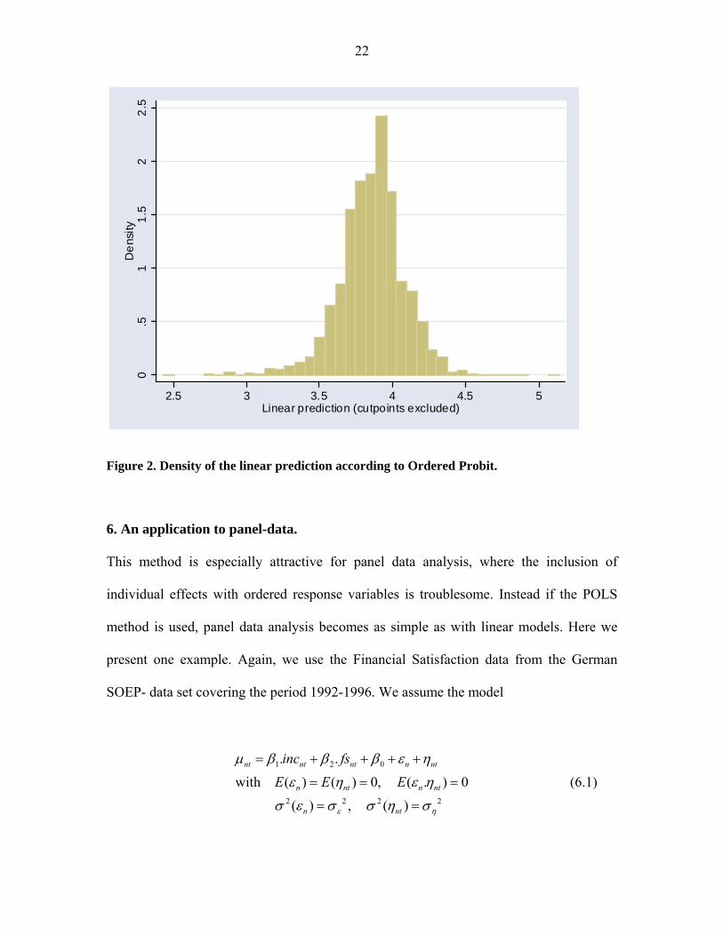
Finally, we look at the distribution of ( )n OPX β′ over the sample. We present the graph of

the distribution in fig. 2, which shows that the distribution looks rather normal indeed.

The usual normality tests on skewness, kurtosis and the Jarque-Bera test do not reject the

normality assumption.

22

0.5

11.

52

2.5

Den

sity

2.5 3 3.5 4 4.5 5Linear prediction (cutpoints excluded)

Figure 2. Density of the linear prediction according to Ordered Probit.

6. An application to panel-data.

This method is especially attractive for panel data analysis, where the inclusion of

individual effects with ordered response variables is troublesome. Instead if the POLS

method is used, panel data analysis becomes as simple as with linear models. Here we

present one example. Again, we use the Financial Satisfaction data from the German

SOEP- data set covering the period 1992-1996. We assume the model

1 2 0

2 2 2 2

. .

with ( ) ( ) 0, ( . ) 0

( ) , ( )

nt nt nt n nt

n nt n nt

n nt

inc fs

E E E

ε η

μ β β β ε η

ε η ε η

σ ε σ σ η σ

= + + + +

= = =

= =

(6.1)

23

The random effect and the white noise are both assumed to be normally distributed. We

estimated the model by Ordered Probit using STATA and by our POLS –approach. We

find the following results, presented in Table 3.

Table 3. Estimates of the same relation by OP and POLS with random effects. Data:GSOEP, 1992-1996 OP, random effects POLS, random effects Coeff. t-ratio Coeff. t-ratio Ln(y) 0.439 21.240 0.669 22.260 Ln(fs) -0.248 -11.170 -0.357 -11.040 Constant 1.955 8.210 Number of observations 25609 25609 Number of individuals 7807 7807 Log.Like. -48172.8 R2: Within 0.002

Between 0.074 overall 0.038

Var (ind. random effect)/ Var (total unexplained) 0.377 0.344

Trade-off-ratio 2 1/β β -0.566 -0.534 The intercept terms are now shown in the table.

As expected, we find again that the two methods lead to similar results. However, there is

a remarkable difference between the running times of the two methods. The traditional

method via standard STATA (using the “reoprob” command) takes about 1.5 hour, while

the POLS approach, using “xtreg” on the transformed answers, requires less than a

minute running time.

For more applications we refer to Van Praag and Ferrer-i-Carbonell (2004), e.g. Chapter

6 with a free error- covariance matrix.

24

7. The link between BI-POLS and the linear probability model.

There is an interesting link between the BIPOLS-model and the so-called linear

probability (LP) -model (see e.g. Heij et al., 2004, p.439). The linear probability model is

of an extreme simplicity. The variable Y is a binary dependent variable assuming the

values 0 and 1. It is assumed that ( 1)P Y = = 0X β β′ + . It is explained by the regression

equation

0Y X β β′= + (7.1)

The serious literature rejects this model for some reasons, notably because the RHS in

(7.1) can assume values outside the interval [0,1]. The model is logically inconsistent.

Nevertheless, the estimation method is frequently used in practice, because it is simple

and the trade-off ratios are remarkably similar to those found with Probit-analysis. Using

our approach we can now understand why this is and must be the case.

Consider the BIPOLS- analogue, where we assign the values 1 2,μ μ to the lower and

upper category, respectively. Averaging over the lower and upper category we find

1 1 0,

2 2 0,

POLS POLS

POLS POLS

X

X

μ β β

μ β β

′= +

′= + (7.2)

Now we remind the reader that the choice of the values 1 2,μ μ depends on the specific

identification rule, where we assumed that the label- variable μ is N(0,1)-distributed. We

25

may use other scaling and position parameters, such that 1 2,μ μ become equal to zero and

one. We solve the system

1 0,

2 0,

0 ( ) .

1 ( ) .

POLS POLS

POLS POLS

X

X

γ β δ β

γ β δ β

′= +

′= + (7.3)

for γ and δ. It follows that if we identify μ by assuming μ to be ( , / )N γ δ γ -distributed,

then BIPOLS is equivalent to the Linear Probability method. As POLS estimates the

trade-off ratios as efficiently as Probit, it follows that LP is just as good as Bi-Probit.

However, this does only hold for the case of two response categories. If we have three

categories and try to estimate in the same way by assigning the values 0,1,2 to the

response categories, the trade-off ratios will be distorted.

8. How about Logit?

In the literature there is an alternative to the Probit model, viz. Logit analysis (see Cramer

(2003) for a recent survey). Up to now there is no definite preference for one of the two

modes. Some researchers like Logit better than Probit and vice versa. It is just a matter of

tradition which method one chooses. Amemiya (1981) suggested that the Logit and

Probit estimators differ only by a multiple of about 0.625 (see also Maddala p.22). He

suggested that this was so, because the two distributions look very much alike. In this

paper we argue that this is just a consequence of the general fact that both are

representations of the same net of indifference curves.

26

A POLS- type approach to Logit is simple to construct. Assume that the representation is

logistic, which implies a logistic distribution function. In that case we may define the

logistic analogue of equation (3.1) by

1( ) ( ) ( 1,..., )i i ip L L i kμ μ −= − = (8.1)

Then we may define the conditional expectations ,ni LOGμ with respect to the logistic. For

the formula we refer to Maddala (1983, p.369). We estimate the model

, ,0

n

m

i LOG i LOG in nZ Xβ ε= +∑ (8.2)

Now the variance of the standard Logit is 213π . It follows that 21

3 .LOG POLSβ π β≈ .

There is one problem which makes the logistic problematic. If the left-hand side of (8.2)

is logistically distributed that must hold for the right-hand side as well. But the first term

at the right hand tends to a normal variate due to the working of the Central Limit

Theorem. This makes (8.2) logically inconsistent. It is for this reason that we do not

recommend the Logit- specification.

9. Discussion and Conclusion.

In this paper we develop a linear –method that compares very well with the traditional

Ordered Probit. The essential point is that we estimate the shape of indifference curves,

that is, the trade-off ratios between coefficients. This method, which we call POLS,

27

replaces the original dependent variable by its conditional mean. This new variable obeys

the same trade-off relations as its underlying component. In the paper we show that the

POLS yields almost the same outcomes as OP, except for a proportionality factor. If that

situation does not hold, the POLS- procedure is attractive for the analysis of ordinal

variables in its own right.

The essential difference between the traditional latent variable approach and our

approach is that traditionally one starts to define the underlying model and its likelihood.

We instead start by translating the observed ordered variable according to its conditional

mean and applying OLS afterwards. In our approach we stay much closer to OLS and

there is only a gradual difference between the treatment of continuously and discretely

observable variables.

In presenting the new method, this paper contributes to the understanding of the Probit

model. This is in itself interesting from a theoretical point of view. Nevertheless, the

POLS method might not seem very relevant for present econometric and statistical

practice, as the Probit- routine is included in most standard software packages. However,

the POLS method is easily generalized to complex situations (such as panel data and

system of equations), which are even nowadays not a matter of computational routine.

For example, consider the multi-Probit version of a SUR model where, say, k equation

errors are correlated, this involves hard computations of k-dimensional integrals on a

large scale. Here we may also use the POLS- trick by replacing all k variables to be

explained by their POLS-analogues and estimating the corresponding SUR-equation

system in a linear setting. We refer to Van Praag, Ferrer-i-Carbonell (2004) and to Van

Praag, Frijters, Ferrer-i-Carbonell (2003) for empirical examples.

28

Another instance where the POLS-approach is very helpful is when we employ Probit

type-variables in longitudinal analysis with inter-temporal correlations. While for ordered

response variables the use of panel techniques becomes difficult (see Greene (2005),

Ferrer-i-Carbonell and Frijters 2004)), such econometric techniques are very easy to

implement if using the POLS method. We again refer to Van Praag and Ferrer–i-

Carbonell (2004) for empirical examples.

The approach is also helpful when we want to employ ordered variables as explanatory

variables. In this case, we can plug in the conditional mean as explanatory variable.

Examples are found Van Praag and Baarsma (2005) and Van Praag and Ferrer–i-

Carbonell (2004). It is a matter of course that the usual identification problems and their

solutions hold. Identification does not become more difficult but not easier either. Next to

the above-mentioned examples, the POLS can also be applied to factor analysis and

principal components.

The most important result of our findings is that a good part of the methods of traditional

discrete response analysis may be replaced by POLS and its generalizations, utilizing a

POLS- transformation of the data. Not only are the OLS-variants computationally easier

than the discrete methods that require the computation of many integrals and or Monte

Carlo simulations, but also they open the way to the application of linear classical

methods to discrete response data.

One thing we should always keep in mind: discrete observation instead of observation on

a continuous scale necessarily implies a loss of information. This loss of information will

have an impact on the standard deviations, which become larger, and on the correlations,

which will become smaller in an absolute sense than under continuous observation. This

29

is the price to be paid for discrete observation. However, this has nothing to do with a

POLS - cardinalization. As we saw, the same loss in reliability has to be paid when

applying a Probit –type method.

30

References:

Amemiya,T.(1981).'Qualitative Response Models: a Survey', Journal of Economic

Literature,19(4),pp.483-536

Blanchflower D., A.J.Oswald, 2004, "Well-Being Over Time in Britain and the USA",

Journal of Public Economics, , 88, 1359-1386

Clark, A.E. and A.J. Oswald, 1994. 'Unhappiness and unemployment'. Economic Journal,

104: 648-659.

Cramèr, H., 1937, Random Variables and Probability Distributions, Cambridge tracts in

Mathematics and Math. Physics 36, Cambridge university Press, Cambridge(U.K.).

Cramer,J.S., 2003, 'Logit Models from Economics and Other Fields', Cambridge

University Press: Cambridge.

G.Debreu, 1959. Theory of value. An axiomatic analysis of economic equilibrium.

Cowles Foundation Monograph No. 17 .New York: John Wiley & Sons

DeMaris,A.,2004 , Regression with social data: Modeling continuous and Limited

response Variables, Wiley and Sons.

DiTella, R., R.J. MacCulloch and A.J. Oswald, 2001. 'Preferences over Inflation and

Unemployment: Evidence from Surveys of Subjective Well-being' American

Economic Review, 91: 335 -341.

Dhrymes (1984), P.'Limited dependent variables',in Z.Griliches and M.Intriligator(Eds.),

Handbook of econometrics,2,Amsterdam:North-Holland Pub.C.

Easterlin, R.A., 2001. 'Income and happiness: Towards a unified theory'. The Economic

Journal, 111: 465-484.

Feller ,W. 1971, An Introduction to Probability Theory and Its Applications, Volume 2,

Wiley & Son, New York.

Ferrer-i-Carbonell, A., 2005. Income and well-being: An empirical analysis of the

income comparison effect. Journal of Public Economics, 89(5-6): 997-1019.

Ferrer-i-Carbonell, A. and P. Frijters, 2004. How important is methodology for the

estimates of the determinants of happiness? The Economic Journal, 114: 641-659.

Frey, B.S, and A. Stutzer, 2002. What can economists learn from happiness research?

Journal of Economic Literature, 40: 402-435.

31

Frijters, P., J.P. Haisken-DeNew, and M.A. Shields. 2004. Money does matter! Evidence

from increasing real incomes and life satisfaction in East Germany following

reunification. American Economic Review.

Greene, W., 2005. Censored Data and Truncated Distributions, forthcoming in The

Handbook of Econometrics:Vol.1, ed. T.Mills and K.Patterson, Palgrave, London.

Heij C., P.de Boer, P.H.Franses, T.Kloek, H.K.van Dijk, (2005).Econometrics Methods

with Applications in Business and Economics, Oxford University Press, Oxford.

Long, S. 1997, Regression models for Categorical and Limited Dependent Variables,

Sage Publications, Thousand Oaks.

Maddala G.S., (1983).Limited –dependent and qualitative variables in Econometrics.

Cambridge University Press.

Pareto, V. (1906). Manual of Political Economy. 1971 English translation.

Rao,C.R.,1973, Linear Statistical Inference and Its Applications, wiley &Sons, New

York.

Ronning, G; M Kukuk (1996),Journal of the American Statistical Association, Vol. 91,

No. 435., pp. 1120-1129.

Stewart, M. (1983). ‘On least squares estimation when the dependent variable is

grouped’. Review of Economic Studies, 50: 141-49.

Terza, J. V. (1987) ‘Estimating linear models with ordinal qualitative regressors’. Journal

of Econometrics, 34(3): 275-91.

Van Praag, B.M.S., 1971. 'The welfare function of income in Belgium: an empirical

investigation.' European Economic Review, 2: 337-369.

Van Praag, B.M.S., (1991). 'Ordinal and Cardinal Utility: an Integration of the Two

Dimensions of the Welfare Concept' , Journal of Econometrics, vol. 50, pp. 69-89

also published in: The Measurement of Household Welfare, R. Blundell, I. Preston, I.

Walker (eds.), Cambridge University Press, 1994, pp. 86-110

Van Praag, B.M.S. and B.E. Baarsma (2005) 'Using happiness surveys to value

intangibles: The case of airport noise', Economic Journal 115, 224-246

Van Praag, B.M.S., and A. Ferrer-i-Carbonell, 2004. Happiness Quantified: A

Satisfaction Calculus Approach. Oxford University Press, Oxford: UK.

32

Van Praag, B.M.S., P. Frijters and A. Ferrer-i-Carbonell, 2003. 'The anatomy of well-

being'. Journal of Economic Behavior and Organization, 51: 29-49.