NASA-CR-201068

Research Institute for Advanced Computer ScienceNASA Ames Research Center

An all-at-once reduced Hessian SQP scheme

for aerodynamic design optimization

Dan Feng and Thomas H. Pulliam

• RIACS Technical Report 95.19 October 1995

https://ntrs.nasa.gov/search.jsp?R=19960029099 2018-06-03T11:59:53+00:00Z

An all-at-once reduced Hessian SQP scheme

for aerodynamic design optimization

Dan Feng and Thomas H. Pulliam

The Research Institute for Advanced Computer Science is operated by Universities Space Research

Association, The American City Building, Suite 212, Columbia, MD 21044 (410)730-2656

Work reported herein was supported in part by NASA under contract NAS 2-13721 between NASA

and the Universities Space Research Association (USRA).

AN ALL-AT-ONCE REDUCED HESSIAN SQP SCHEMEFOR AERODYNAMICS DESIGN OPTIMIZATION*

DRAFT

by

Dan Feng t and Thomas H. Pulliam_

*Work reported herein was supported by NASA under contract NAS 2-13721 between NASA and the

Universities Space Research Association (USRA).

lResearch Institute for Advanced Computer Science (RIACS), Mail Stop T20G-5, NASA Ames Research

Center, Moffett Field, CA 94035-1000, USA. (feng@riacs.edu)

tFluid Dynamics Division, Mall Stop T27B-1, NASA Ames Research Center, Moffett Field, CA 94035-

1000, USA. (pulliam_nas.nasa.gov)

Abstract

This paper introduces a computational scheme for solving a class of aerodynamic

design problems that can be posed as nonlinear equality constrained optimizations. The

scheme treats the flow and design variables as independent variables, and solves the con-

strained optimization problem via reduced Hessian successive quadratic programming.

It updates the design and flow variables simultaneously at each iteration and allows flow

variables to be infeasible before convergence. The solution of an adjoint flow equationis never needed. In addition, a range space basis is chosen so that in a certain sense

the "cross term" ignored in reduced Hessian SQP methods is minimized. Numerical

results for a nozzle design using the quasi-one-dimensional Euler equations show that

this scheme is computationally efficient and robust. The computational cost of a typ-

ical nozzle design is only a fraction more than that of the corresponding analysis flow

calculation. Superlinear convergence is also observed, which agrees with the theoretical

properties of this scheme. All optimal solutions are obtained by starting far away fromthe final solution.

Key words, design optimization, constrained optimization, reduced Hessian meth-

ods, quasi-Newton methods, successive quadratic programming

AMS(MOS) subject classification. 65K05, 90C06, 90C30, 90C31, 90C90

Abbreviated title. SCHEME FOR DESIGN OPTIMIZATION

1 Introduction

An aerodynamic design optimization problem can often be posed as

min l(X,u) (1.1)s.t. F(X, u) = O,

where X E _n denotes the discretized flow variables, and u E _m denotes the design

variables, which, for example, could be geometry parameters describing the shape of a

profile; I : _,_+m __+ _ is a cost function, which may, for example, measure the deviation

from a desired surface pressure distribution; F : _n+m _. _n is a discretized version of the

governing equations of the flow field. It is often the case that I and F are nonlinear, and

the number of flow variables is much larger than the number of design variables (n > > m).

Many computational methods for solving (1.1) have been developed, and each seeks to

find the solution by solving a series of subproblems. One can categorize these methods by

looking at how the design and flow variables are treated. In one category, design optimiza-

tion approaches treat X as a dependent variable of u. Representatives in this category are

the brute-force approach, the implicit gradient approach (e.g. [18]) and the adjoint equa-

tions approach (e.g. [14]). These approaches have a feasibility requirement that is satisfied

by solving the nonlinear flow equations to convergence in each design cycle. They only

differ in how V,,I is calculated at each iteration. The brute-force approach computes _7,,I

by one-side finite differences, which requires m solutions of the flow equations. The implicit

gradient approach and the adjoint equations approach also require at least two solutions of

nonlinear flow equations at each design iteration.

In another category, design optimization approaches treat X and u as independent

variables. Given Xk, uk, each approach in this category finds AXk, Auk and updates all

the variables at once such that Xk T AXk, uk q- Auk better solves (1.1), and iterates until

a satisfactory solution is obtained. One interesting property is that the flow equations are

not required to be satisfied until convergence. Approaches in this category are expected to

mitigate the computational cost of repeatedly solving the nonlinear flow equations required

by other methods. The success of flow solvers based on Newton's method (e.g. see Barth

[1] and [13]) also makes the all-at-once approach more tractable.

The approach introduced in this paper belongs to this latter category. Methods that

simultaneously update design and flow variables have been studied by many authors in-

cluding Frank and Shubin [7], Huffman et al [13], and Hou et al [12]. The scheme in [13] is

based on Successive Quadratic Programming (SQP) for equality constrained optimization.

In their scheme the Hessian matrix is approximated by selectively calculating some second

order terms instead of using an update formula. The calculation of second order terms

could be prohibitive in many situations. The formulation introduced in [12] is based on

successive linear programming. This scheme may suffer from convergence problems and

in addition a linear adjoint system has to be solved at each iteration. Frank and Shubin

[7] compare three optimization-based methods, including an all-at-once scheme (based on

the full Hessian SQP that would be too expensive to form for large problems) for solving

aerodynamic design problems. They point out, however, that an all-at-once scheme could

be very efficient if carefully implemented.

SQP is a mature and successful technique for solving nonlinear constrained optimization

problems due to its relatively low computational cost and fast convergence. However, it is

not widely used in aerodynamic design optimization. The major obstacle is that aerody-

namic design optimization problems are often very large. In order to have an efficient and

robust implementation of SQP methods, one has to take full advantage of special character-

istics of the aerodynamic design problems. This paper is intended to address some aspects

of this issue.

Since the approach introduced in this paper originates from SQP for equality constrained

optimization, we first describe the full Hessian SQP scheme in the context of (1.1).

At each iteration of SQP methods, a quadratic approximation to the Lagrangian function

of (1.1)

L(X, u, A) = I(X, u) + ATE(X, u),

is minimized subject to a linearization of the flow equations. This gives a subproblem

minde_,,+m ) gTd + l dT Hkd (1.2)

subject to Fk + ATd = 0, (1.3)

where d = gk = _ at (Xk, uk), Ak = at (Xk, u_), Fk = F(Xk, Uk),

and //k is the Hessian (or approximation) of the Lagrangian function.

2

Onedifficulty implementing full SQP methods for aerodynamic design optimization is

that the analytic Hessian of the Lagrangian is usually hard to obtain. Another difficulty

is that approximating the Hessian by update schemes tends to create large dense matrices((n + ,_) x (n + ,_)).

These difficulties can be overcome by dropping certain non-critical second order infor-

mation. This idea has been pursued by many researchers including Coleman and Corm [4],Nocedal and Overton [16], Byrd and Nocedai [3]. We illustrate the basic idea as follows.

One way of solving (1.2-1.3) is via separation of variables. Suppose we can compute two

matrices Yk E _(n+m)xn and Zk E _(n÷m)xm such that the matrix [Yk Zk] is nonsingular

and ZTAk = 0 (Zk is a basis for the null space of AT). Let d = Ykdl + Zkd2 and plug this

into (1.2-1.3). If we assume ZTHkZk is positive definite (which is reasonable because this

matrix is indeed positive definite close to the solution due to the second order sufficient

optimality condition), by standard techniques, dl and d2 are given by

dl = --(ATyk)-I Fk

d2 = -( ZT Hkzk)-'(zT gk + ZT HkYkdl).

To avoid the computation of Hk, the "cross" term ZTHkYkdl is simply ignored andzTHkzk is approximated by an m × m matrix Bk using a variable metric formula such as

BFGS. Consequently,

d, = -( ArkYk)-' rk (1.4)

d2 = -Bk 1ZTgk. (1.5)

Methods based on (1.4-1.5) are referred to as reduced Hessian SQP methods.

The biggest advantage of reduced Hessian SQP methods for aerodynamic design opti-

mization is that only a small m x m matrix holding second order information needs to be

maintained and updated. Theoretically, reduced Hessian SQP methods are not as effective

as full Hessian SQP methods. However, many versions are shown to have 2-step superlin-

ear local convergence (for example see [16], [3] and [19]), which is good enough for mostapplications.

One challenge of implementing (1.4-1.5) for aerodynamic design optimization is the

choice of Zk and Yk. Traditionally, Zk and Yk are chosen from an orthonormal matrix

obtained from the QR factorization of Ak. QR factorization based reduced Hessian SQP

algorithms are proven to be very robust in practice (for example, see [11]). However, for

aerodynamics design optimization, Ak contains the flow Jacobian matrix, which is usually

very large. Orthonormal base are usually too expensive to compute.

Many authors, including Gabay [8], Gilbert [9], Fletcher [6], and Xie and Byrd [19], have

proposed more economical choices of Zk and Yk which are not orthogonal. One popularchoice of Zk is

-_J _'$'_'_J (1.6)Zk = I = '

where,in caseof aerodynamic design optimization, S is the sensitivity matrix. It can easily

be verified that ZTAk = 0. The calculation of the sensitivity matrix is usually affordable

for many applications. An economical choice of Yk is [I 0]T, which is used by many authors

including niegler et al [2], and Dennis et al [5].

This paper introduces a reduced Hessian SQP scheme for the aerodynamic design prob-

lem (1.1). Equations (1.4-1.5) are used to compute a trial step at each iteration. The

popular choice of Zk given by (1.6) is used. However, a different choice of Yk is considered.

We show that using [I 0]T has an undesirable effect of potentially producing a larger cross

term. Here Yk is chosen such that ZTyk = 0 holds, which in a certain sense will minimizethe cross term. We also show that this choice of Yk has the advantage of gaining accuracy

in the reduced Hessian approximation, which is very important for ensuring the reliability

and robustness of a reduced Hessian SQP scheme.

The new scheme is implemented and tested on the shape design of a transonic nozzle.

The transonic flow through the nozzle with a given area ratio is governed by the quasi-one-

dimensional Euler equations. The transonic conditions which generate a shock within the

nozzle present a difficult test case, where methods typical of practical aerodynamic applica-

tions are required. Such methods include, finite difference, finite element, and unstructured

grid finite volume techniques employing various forms of highly nonlinear algorithm con-structions.

This paper is organized as follows. First the all-at-once reduced Hessian SQP scheme is

introduced in Section 2. The solution of the quasi-one-dimensional Euler equations for flow

through a nozzle with a given area ratio is discussed in Section 3. Section 4 first describes

the design optimization problem used in our testing, then provides computational results

and the performance evaluation of the new scheme on the design problem. The testing is

carried out by using different numbers of design variables (spline coefficients for the nozzle

shape) for the test problem. Finally, we give some concluding remarks in Section 5.

2 An all-at-once reduced Hessian SQP scheme

Let Bk be an approximate to Z[HkZk. Let Zk be given by (1.6). We define Yk by

(i)Yk---- S T •

Clearly zTYk = 0 holds.

Let d = Ykdl + Zkd2.

(2.1)

Replacing the reduced Hessian matrix by Bk and ignoring the

cross term in (1.5), we have

d2 = - B kl Z[gk.

From (1.4), dl satisfies (ATyk)dl = -Fk, which is equivalent to

\-_,] -[-_OU] ST dl -_ --Fk,

which in turn is equivalent to

dk(I + sST)dl = --Fk, (2.2)

where dk = at (Xk, uk) is the current Jacobian matrix of the flow equation. Equation

(2.2) can be solved by first solving dky = -Fk for Y, and then solving (I + sST)dl = Y for

dl. The solution of the former is simply the Newton step calculation from the flow equations

at the current iteration, which can be provided by any Newton's method based flow solver.

The solution of the latter can be obtained by the conjugate gradient method, which is

guaranteed to converge within (m + 1) iterations due to Rank(SS T) = m (see Golub and

Van Loan [10]). Another way of solving (I + sST)dl = y is by inverting (I + SS T) directly.It is easy to show that

(I + ssT) -1 - I - S(I + STS)-IS T.

Note that (I + STS) is only an m x m matrix and its factorization can be obtained atminimal cost.

After dl and d2 are available, d is given by

d

d2.

A erwardsweupdateoursolution("l)(Xk)odupd te andtheulLangrange multiplier Ak (which is used implicitly in the merit function calculation, see

below), and go to next iteration.

The Lagrange multiplier is asked to satisfy

(yTAk)Ak = -Y_'gk, (2.3)

which is equivalent to

(z + ssZ)(dr k) = -V[gk.

As a matter of fact, we will see that our scheme only needs the value of (JTAk).

We establish the following lemma that is useful to us.

Lemma 2.1 Let M, N E R n×'n with n > m. If M and N have the same range space of

dimension m, then

M(NTM)-IN T = M(MTM)-IM T. (2.4)

Proof. Clear (NTM) is invertible. Since M and N have the same range space,

M(MTM)-IM T = N(NTN)-IN T. (2.5)

Postmultiplying each side by M(NTM)-IN T and using (2.5) gives

M(MTM)-IMTM(NTM)-IN T = N(NTN)-INTM(NTM)-IN T

M(NTM)-IN T = N(NTN)-IN T

which gives (2.4) using (2.5). []

When certain update criteria are satisfied, the Hessian approximation update is carriedout via the BFGS formula

Bk_ks_rBk YkY[ (2.6)Bk+l = Bk sTBksk + yTs k,

where

Yk = zT+1[V(X,,,)L(Xk+I, Uk+l, _k) -- _7(X,u)L(Xk, Uk,/_k)] (2.7)

T -1 TSk = (Zk+lZk+l) Zk+lO_d, (2.8)

with a being the step length resulted from a line search. This choice of Yk, Sk pair is

among the choices recommended by Nocedal and Overton [16]. From the definition of the

Lagrangian function

Yk = zT+l[(gk+l + Ak+_k) -- (gk + Ak,_k)]

= zT+,[gk+l -- (gk -- Ak(yTAk)-IyTgk)]

= ZT+l[gk+l - (I - rk(yTrk)-lYkT)gk ]

= z/+,[gk+_- zk(z[zk)-lz[g_l.

(2.9)

(2.10)(2.11)

Equation (2.9) to (2.10) is due to Lemma 2.1. Equation (2.10) to (2.11) is because

z,(z[zk)-'z[ + rk(r/rk)-'r/= i

due to zTYk = O.

To ensure convergence, a merit function is needed to monitor the progress towards the

solution. We choose to use the 11 merit function for its simplicity and low computational

cost. The 11 merit function is defined as

¢_(x, u) = l(X, u) + _IIF(X, _)11,.

The directional derivative of ¢_ along d is given by

D¢, k(X, u; d) = g[d - _kllFklla. (2.12)

6

Pluggingd = Ykdl + Zkd2 into (2.12) yields

D_.k (X, u; d) = g[gkdl + g[Zkd2 - _kllFklh.

Clearly, on the one hand

g_Zkd2 -Tz B-1Z T-=-Yk k k kYk<0, (2.13)

since Bk is forced to be positive definite. On the other hand, from (2.3) and dl =-(rlak)-lFk,

gTykdl = AT Fk = (JT Ak)T(j-1Fk). (2.14)

Note that both (JTAk) and (J-1Fk) are available from previous calculations. From (2.13-

2.14)

D_,,k (X, u; d) < 0

can be guaranteed by choosing #k > ()_TFk)/]]FklI1

We point out that jT is not needed in the entire scheme, which is desirable in aerody-namic calculations.

One feature of our choice of Yk is that the cross term ignored in the reduced Hessian

SQP formulation is likely to be minimized. Since this is not a obvious claim, We establishthe following lemma.

Lemma 2.2 For a given matrix N E _nxm and a vector p E _m, over all the choices of

matrices i E _x_ such that ( NTM ) is invertible, IIM (NTM )-_pl I is minimized if i hasthe same range space as N.

Proof. Let N = UDV T be the singular value decomposition of N with U E _,_x,,_ and

D,V E R,_xm, and M = QR be the QR decomposition of M with Q E R,_xm and R E

Rmx,_. Clearly, D and R have full rank. Then

[[M(NTM)-lp[[ = [[QR(VDUTQR)-Ip][ = [[Q(UTQ)-ID-1VTp[[

= [[(uTQ)-_D-1VTp[[ >_ [[D-_yTp[[/a,,,a_, (2.15)

where a,_ax is the largest singular value of (UTQ). Since U and Q are unitary, [[UTQ[[ <_[[uT[[[[Q[[ = 1, which implies a,n_x _< 1. Hence

[[M( NT M)-lp[[ >_ [[D-1VTp[[.

The equality is achieved when UTQ is unitary (in this case ama_ = 1. Hence it is sufficient

to show that UTQ is unitary if M and N have the same range space.

Clearly if M and N have the same range space, then Q and U have the same rangespace. Since Q and U are unitary, QQT = UU T holds. Therefore

(UTQ)T(uTQ) = Qr(uUT)Q = QT(QQT)Q = (QTQ)(QTQ) = I,

7

whichimpliesthat UTQ is unitary. []

Recall that dl = --(ATyk)-IFk. Choosing Yk such that zTYk = 0 implies that Yk and

Ak have the same range space due to ZTAk = O. Hence by aemma 2.2, ]lYkdlH achieves

minimum value when zTYk = O. For a given Zk and Hk, a smaller ]]Ykdl ]1is desirable since

it has a major contribution to the magnitude of the cross term ZTHkYkdl ignored in thereduce Hessian formulation.

Choosing Yk such that zTyk = 0 also has the potential advantage of improving accuracy

in the Hessian approximation. Note that (2.8) implies

7" )-l Z[+lo, d.Zk+l sk = Zk+_ (Zk+l Zk+_

The Taylor expansion of Yk used in the step secant update gives

T 2Yk = Zk+l V(x,u)(x,,_)L(Xk, uk, Ak)ad + O([[ad[[ 2)

T 2= Zk+ 1V(X,_,)(x,_ )L(Xk, uk, Ak)Zk+3 (zT+3 Zk+3 )-3 ZT+lad

T 2 )-3 Z[+3 )o_d- Zk+3 (Zk+3 Zk+l-[- Zk + l V ( X,u)( X,u) L( X k, Uk, ,_k )( I T

+o(ll-dH :)T 2

= Zk+3V(X,_)(X,,,)L(Xk, uk, Ak)Zk+lSk

_}_Z T 2k+3 V (x,u)(x,_,)L( Xk, uk, Ak)Yk+3 (YkT+3Yk+3 )-lykT+3 ad + O(lladll2).

Since Bk+3 is expected to approximate the reduced Hessian matrix, it is desirable to keep

the size of the second term as small as possible. This goal can be partially achieved by

controlling the size of Yk+i(Y[+3Yk+3)-lYkT+3 d. Using d .: Ykdl + Zkd2, we have

II(Yk+,(Y_ Yk+3 )-1 Yk_l )dll

= II(Yk(yTyk)-3yT)dII + O(lldll2)

= IlYkd3+ (Yk(YTYk)-IYT)Zkd2II + O([Idl12). (2.16)

Choosing Yk such that zTYk = 0 makes IIYkd311 achieve its minimum value as analyzed

above, and makes II(Yk(Y[Y_,)-3Y[)Zkd211 zero. Hence it is likely that this choice would

yield the lowest value for (2.16).

3 Quasi-one-dimensional Euler equations

For our purposes here, we have chosen one popular form of central finite differences with

nonlinear artificial dissipation applied to the quasi-lD Euler equations.

The quasi-lD Euler equations are

F(Q) = 0=E(Q) + H(Q) + D(Q) = 0 0.0 _< x _< 1.0 (3.1)

where

q 1 [0, E=a(x) pu 2+p , I-I= -pO=a(x)

u(e + p) J o(3.2)

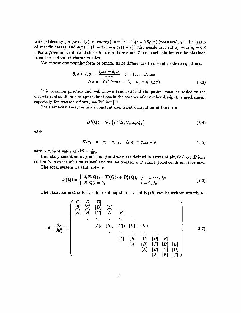
with p (density), u (velocity), e (energy), p = (7- 1)(e-0.Spu 2) (pressure), 7 = 1.4 (ratio

of specific heats), and a(x)= (1.- 4.(1- at)x(1- x))(the nozzle area ratio), with at = 0.8

. For a given area ratio and shock location (here x - 0.7) an exact solution can be obtainedfrom the method of characteristics.

We choose one popular form of central finite differences to discretize these equations.

a:_q ,_ _f_qj - qj+l - qj-12Az j = 1,...,Jmax

Ax = 1.o/(gmax- 1), uj = u(jAx) (3.3)

It is common practice and well known that artificial dissipation must be added to the

discrete central difference approximations in the absence of any other dissipative mechanism,

especially for transonic flows, see Pulliam[17].

For simplicity here, we use a constant coefficient dissipation of the form

(3.4)

with

"_qj = qj -- qj-1, A_qj = qj+l - qj (3.5)

with a typical value of _(4) --V_'I

Boundary condition at j = 1 and j = Jraax are defined in terms of physical conditions

(taken from exact solution values) and will be treated as Dirchlet (fixed conditions) for now.The total system we shall solve is

f _xE(Q)j - H(Q)j + D4(Q), j = 1,..., JNY-(Q)

( B(Q)i = 0, i = 0, JN(3.6)

The Jacobian matrix for the linear dissipation case of Eq.(5) can be written exactly as

0Y"A-

0Q

[C] [D] [E]

[B] [C] [D] [E]

[A] [B] [C] [D] [E]

"°. ".. °.. ",. °..

[A]i [B]j [C]j [D]j [S]i

"°° ".. ".° °.° ".

[A] [B] it] [D][A] [B] [C]

[A] [B][A]

[E][D] [El[C] [D][B] IV]

(3.7)

wheretheelements([I] is the 3 × 3 identity matrix) aredefinedas

[A]_ = _(4)[I]

[B]j = -4e(4)[I]- 2-_x [AJ]j

[c]j = 6_(')[I] + [cJ]j

[D]j = -4e(')[I] + &[AJ]j

[S]j = _(')[I]

with

0 1 0 ](3'- 3)u2/2 -(3'- 3)u (7- 1)

[AJlj=a(x)J [-7ue/p+(7-1)u 31 [7e/p-3(7-1)u 2] 7u Jj

(3.s)

and

0 0 0 ][CJ]j = -Oxa(x)j (7- 1)u2/2 -(3'- 1)u (7- 1) (3.9)

0 0 j

The O:_a(x)j term is done with central differences and there are some slight modifications

to the dissipation terms near the boundaries.

4 Test results for a nozzle design problem

The nozzle design problem. We assume that a target velocity distribution u_, is given

for each computational grid. The design problem we are trying to solve is

Find Yi, i = 1,.-., m (spline coefficients describing a(x)), such that1 r"_Jmaxe

2._j=l (uj - u_ )2 is minimized subject to (3.6) being satisfied.

For our test examples, the breakpoints of the spline are evenly distributed in the interval

[0, 1].Some implementation issues. Each design is started from a flat nozzle and a flat flowsolution. The first reduced Hessian approximation is given by Bo = ZTZo.

A trial step d is calculated as described in Section 2. A quadratic backtracking line search

is carried out using the 11 merit function, which yields a step length ak. The following update

criterion is used for the reduced Hessian approximation. At iteration k, Bk is updated using

the BFGS formula (2.6) if

aTyk > O.lo_kllYkdlll. (4.1)

10

Otherwise,we set Bk+l = Bk. This criterion is devised to guard against loss in accuracy

of Bk, as recommended by Xie and Byrd [19], and is critical for ensuring convergence of a

reduced Hessian SQP algorithm.

We give test results on design problems with zero, two and ten design variables. Through-

out this section the number of grids Jmax is set consistently to 67. We chose this number

since having an even breakpoint distribution for the splines requires that (Jmax - 1) bedivisible by the number of design variables plus one. Hence each problem has 67 x 3 = 201

flow variables, and the same number of constraint equations. The convergence was moni-

tored by IINkgkll + IIFkll (llFkll in case of zero design variables), where gk = Zk( Z T Zk )-I Z T

is a projector onto the null space. This quantity indicates how well the first order necessary

optimality conditions are satisfied, and should be zero at the true solution. The toleranceis set to 10 -7 .

b'lm¢ Salem_j _ _ I_mimw P,tw_l

!

j0 iiI0J$ 0_4 025 0_e ? • • 0 2 4 $ II 10 12 14 ldl 111 2t)

(a) (b)

Figure 1: Computational results without design variables. (a) Target (dash line) and final

(checked solid) ttow solutions. (b) Convergence of norm of residual versus iterations.

Test results without design variables. These results are obtained by calling the flow

solver with the optimal nozzle area ratio. We include these results as a baseline for mea-

suring the cost of our optimization scheme. These results are also useful for examining the

effect of the presence of design variables on the flow solution. The overshooting in the final

solution can be controlled by nonlinear dissipation, as described in Pulliam [17].

Figure 1 (a) gives the final and target flow solutions. Figure 1 (b) shows the convergence

history of the nonlinear flow residual versus the iterations. Figure 2 gives snapshots of partial

solutions at various iterations. It can be seen that the transition is quite violent due to theexistence of a shock in the solution.

Test results with two design variables. For this problem four spline coefficients are

used. We keep the coefficients at the end points fixed, leaving the area ratios at the two

between points as design variables. Figure 3 gives the test results for this case. Figure 3 (a)

shows the initial, final and target flow solutions. Figure 3 (b) shows the initial, final and

11

aq a7 o_ a, as Qi ay Qa al

a, u_ _ a4 a_ H a7 ue altJv,_ _ _a

'!l|"

u

QT

0

al a_ os od o$ no o_ ne oeL_4m _me o,,_

e ,

oc" ol a_ o,) _, as o* a_ ao ag

Figure 2: Snapshots of flow solutions at various iterations without design variables Dashed

line - target solution; Checked solid line - current solution.

target nozzle solutions. Figure 3 (c) gives the convergence history of the objective function.

Figure 3 (d) plots the convergence history of the quantities lINkgkll and IIFkll.

The optimization converged quite rapidly taking 14 iterations. Figure 3 (a) and (b) showthat the final flow and nozzle solutions match we]] to the corresponding target solutions.

Figure 3 (c) shows that interates converged to a Kuhn-Tucker point (point that satisfies

first order necessary conditions) superlinearly.

Test results with ten design variables. For this problem twelve spline coefficients are

used. Again we keep the coefficients at the end points kept fixed, leaving the area ratios at

the ten between points as design variables. Figure 4 gives the test results for this case.

It took 30 iterations for the optimization process to converge to the given tolerance.

Figure 4 (a) and (b) show that the final flow and nozzle solutions match well to the corre-

sponding target solutions.The convergence is slower than the case with two design variables. We believe that this

is partially due to over-parameterization that makes the design problem much harder to

solve. Nevertheless, as shown in Figure 4 (d), it converged rapidly (superlinearly) to the

solution after wandering around for a relatively longer transient period.

For the situation with two design variables, it was observed that flow solutions went

through a less violent transient regime compared to the situation when running the flow

solver without the presence of design parameters. For the situation with ten design variables,

similar phenomena occurred. Figures 5 and 6 give some snapshots of intermediate flow

and nozzle solutions with ten design variables at various intermediate iterations. These

snapshots indicate that the transient is much milder with the presence of design variables.

12

o_ o, o, o_ o_ o_ oI_ 0'7 010 '0_

(a)0J

£

i i | : : I

2 4 $ 8 10 12 14

(c)

Nozse SoMI_

1......................................

0.|

i0781 _ I

L_r_ Am_l C_u_

(b)

Jlf4F

(d)

Figure 3: Computational results with 2 design variables. (a) Target (solid line), initial

(dashed line) and final (checked solid) flow solutions. (b) Target (solid line), initial (dashed

line) and final (checked solid line) nozzle profiles. (c) Reductions in objective function. (d)Reduction in projected gradient (+) and flow residual (*).

We suspect that this is partially due to the fact that an intermediate partial nozzle solution

actually helps the flow solver to locate the shock and to estimate its magnitude.

Cost comparisons. Finally, we discuss the performance of the reduced Hessian SQP

scheme with respect to the pure analysis (solution of nonlinear flow equations). Table 1indicates that optimization with two design variables is only slightly more expensive than

the analysis (costing 1.37 nonlinear flow solves). For the same problem, a brute force finite

difference approach would require 3 nonlinear flow solves for a single optimization iteration.

To solve the design problem, the number of nonlinear flow solves required by either an

implicit gradient method or an adjoint equations approach would be at least twice as much

as the number of optimization iterations which may easily exceed 10. For the situation with

ten design variables, a fairly tough problem due to over-parameterization, the performance

13

> 0.a

0.7

0.4

0.6

..4.

-t,g

-2.9

Flow S_qlon

0.t 0.2 0_ 0.4 0.15 0.4 0.7 0.1 0-9Lwq_ _e0 0u,

(a)

a .......$ 10 16 24 _ 34

(c)

No _te 8okallon1.06,

I_ ......................................

OJSl

eJq

°'_' 0', ot o_ o'., o; o'o o', o', o;

(b)

,'o ', ;o _,

(d)

Figure 4: Computational results with 10 design variables. (a) Target (solid), initial (dashed)

and final (checked solid) flow solutions. (b) Target (solid), initial (dashed) and final (checked

solid) nozzle profiles. (c) Reductions in objective function. (d) Reduction in projected

gradient (+) and flow residual (*).

of the reduced Hessian SQP scheme is still reasonably good. It costs an equivalent of

8.217 nonlinear flow solves, which would compare favorably over the other three methods

mentioned above for similar reasons.

5 Concluding remarks

An efficient and robust reduced Hessian SQP scheme for aerodynamic design optimization

has been introduced in this paper. This scheme requires neither the solution of an adjoint

equation nor any exact second order information. The optimization was able to converge

from tough starting points. Computational results show that this scheme has a potentialto achieve the same order of cost as one nonlinear flow solve. However, much more work

14

hi. ht_m i _,_1. _ nm lelmma_lm2r

a_ u _ _4 04 uo ov ul QI

_m_N_. he. Sma_. _vae. ao

al u u m_ a_ De ar al al_qm_m_

°%I ol o_ o._ 04 o_ os sT oe oe

all ol _ u a4 a_ el Q'y ' 'ne uu.qm *me o_

Figure 5: Snapshots of flow solutions at various iterations. Solid line - target solution;Checked solid line - current solution.

Number of Design Variables TotM Flops Number oflterations Cost R_tio0 2142176 20 1.000

2 2935839 14 1.370

10 17602144 30 8.217

Table 1: Efficiency of the all-at-once scheme

is still needed before we have a practical scheme. We believe the efficiency of this scheme

can be improved if combined with grid sequencing [20] or multigrid techniques [15]. These

techniques give efficient ways of providing a good starting point for the design on the final

mesh. Issues such as dealing with inequality constraints and applications to 2D and 3D

problems are currently under investigation.

References

[1] T. BARTIt, An unstructured mesh Newton solver for compressible fliud flow and its

parallel implementation, AIAA Paper 95-0221, (1995).

[2] L. T. BIEGLER, J. NOCEDAL, AND C. SCHMID, A reduced Hessian method for larye-

scale constrained optimization, Tech. Rep. CRPC-TR93432, Center for Research on

Parallel Computation, Rice University, Houston, Texas, 1993.

15

al o_ o_ 0+ al ae o_ oI alti_tm tm0 t_s_

</!

.:ol a2 o,_ 04 as oo 07 oe oe

t J,_ _va,e c_

ws_v.m_Ii

i'aB

i/ll nl 02 o.1 04 ol |i a_ ol I!

temll A_O _

kela+ hv_ d ll._ Jo

+ O%

,K /i

IOY_l+ 01 O+ N:) 04 Ol Ol |t Ol Ol

t.mem A_ _

Figure 6: Snapshots of nozzle solutions at various iterations. Solid line - target solution;

Checked solid line - current solution.

[3] R. H. BYRD AND J. NOCEDAL, An analysis of reduced Hessian methods for constrained

optimization, Math. Programming, 49 (1991), pp. 285-323.

[4] T. F. COLEMAN AND m. CONN, On the convergence of a quasi-Newton method for the

nonlinear programming problem, SIAM J. Numer. Anal., 21 (1984), pp. 755-769.

[5] J. E. DENNIS, M. HEINKENSCIILOSS, AND L. N. VICENTE, Trust region interior-point

algorithms for a class of nonlinear programming problems, Tech. Rep. CRPC-TR95512,

Center for Research on Parallel Computation, Rice University, Houston, Texas, 1995.

[6] R. FLETCHER, Practical Methods of Optimization, Second Edition, John Wiley _z Sons,

second ed., 1989.

[7] P. D. FRANK AND G. R. SttUBIN, A comparison of optimization-based approaches

for a model computational aerodynamics design problem, Journal of Computational

Physics, 98 (1992), pp. 74-89.

[8] D. GABAY, Reduced quasi-Newton methods with feasibility improvement for nonlinearly

constrained optimization, Mathematical Programming Studies, 16 (1982), pp. 18-44.

[9] J. C. GILBERT, Maintaining the positive definiteness of the matrices in reduced Hessian

methods for equality constrained optimization, Math. Programming, 50 (1991), pp. 1-

28.

[10] G. H. GOLUB AND C. F. V. LOAN, Matrix Computations, The John Hopkins Univer-

sity Press, second ed., 1989.

16

[11]

[12]

[13]

[14]

[15]

[16]

[17]

[18]

[19]

[20]

C. B. GURWlTZ AND M. L. OVERTON, Sequential quadratic programming methods

based on approximating a projected Hessian matrix, SIAM J. Sci. Stat. Comput., 10

(1989), pp. 631-653.

G. W. Hou, A. C. TAYLOR, III, S. V. MANI, AND P. A. NEWMAN, Formulation

for simultaneous aerodynamic analysis and design optimization. Manuscript, 1993.

W. P. HUFFMAN, R. G. MELVIN, D. P. YOUNG, F. T. JOHNSON, J. E. Busso-

LETTI, M. B. BIETERMAN, AND C. L. H1LMES, Practical design and optimization in

computational fluid dynamics, AIAA Paper 93-3111, (1993).

A. JAMESON, Aerodynamic design via control theory, Journal of Scientific Computing,

3 (1988), pp. 233-260.

G. KURUVILA, S. TA'ASAN, AND M. D. SALAS, Airfoil design and optimization by

the one-shot method, AIAA Paper 95-0478, (1995).

J. NOCEDAL AND M. L. OVERTON, Projected Hessian update algorithms for nonlin-

early constrained optimization, SIAM J. Numer. Anal., 22 (1985), pp. 821-850.

T. PULLIAM, Artificial dissipation models for the Euler equations, AIAA Paper 85-

0438, (1985).

G. R. S HUBIN, Obtain 'cheap' optimization gradients from computational aerodynamics

codes, Tech. Rep. AMS-TR-164, Boeing Computer Services, Seattle, Washington, 1991.

Y. XIE AND R. H. BYRD, Practical update criteria for reduced Hessian SQP, Part I:

Global analysis, Tech. Rep. CU-CS-753-94, Computer Science Department, University

of Colorado, Boulder, 1994.

D. P. YOUNG, W. P. HUFFMAN, M. B. BIETERMAN, R. G. MELVIN, F. T. JOHN-

SON, C. L. HILMES, AND A. R. DUSTO, Issues in design optimization methodology,

Tech. Rep. BCSTECH-94-007 REV. 1, Boeing Computer Services, Seattle, Washing-

ton, 1994.

17

RIACSMail Stop T041-5

NASA Ames Research Center

Moffett Field, CA 94035