AMSC 664 Final Report: Upgrade to the GSP

Gyrokinetic Code

George Wilkie (gwilkie@umd.edu)Supervisor: William Dorland (bdorland@umd.edu)

May 14, 2012

Abstract

Simulations of turbulent plasma in a strong magnetic field can, insome cases, take advantage of the gyrokinetic approximation, the resultof which is a closed set of equations that can be solved numerically. Anexisting code, GSP, uses a novel and highly efficient solution method. Inthis project, we change the velocity-space representation in GSP. Thistransformation will eventually make the algorithm more suitable for sim-ulations of turbulence in Tokamak plasmas, while retaining the efficiencyand accuracy of the original code.

1 Background

Plasma physics concerns the collective dynamics of collections of many chargedparticles interacting self-consistently with their respective electromagnetic fields.In a uniform magnetic field, the motion of a charged particle (we are usuallyreferring to ions unless otherwise specified) in the plane perpendicular to themagnetic field is a circle whose radius (the gyroradius ρ) depends on its velocityin that plane:

ρ =v⊥Ω

(Ω is the gyrofrequency). If this radius is much smaller than the characteristicsize of the plasma, we can use that ratio as an expansion parameter. Gyroki-netics specifically is the regime in which turbulent fluctuations can be aboutthe size of this gyroradius. This is in contrast to drift-kinetic theory (and byextension, MHD), where the gyroradius needs to be much smaller than the sizeof the fluctuations. In order to get a closed theory in gyrokinetics, we demand

that the drift velocity be small compared to the thermal velocity vt ≡√

Tm .

Such drifts come about when there is curvature or a gradient in the magneticfield or if there exists another force field (such as the electric field).

We can summarize the gyrokinetic assumptions thusly:

ρ

L∼ vE

vt∼ ω

Ω∼ ν

Ω∼ ε 1

1

Here, vE = EB0

is the E × B drift speed, ω is the frequency of turbulent fluc-tuations, and ν is the characteristic collision frequency. These assumptions arewell justified in plasmas found in magnetic fusion confinement devices and inastrophysical plasmas.

The gyrokinetic equation results from expanding the distribution functionin the small parameter ε ≡ ρ

L :

f(r,v, t) = F0 + εδf + . . .

Where δf represents the fluctuations in the distribution function, which is inturn responsible for fluctuations in density, flux, and temperature, and all per-turbed fields that depend thereon.

The function we will be solving for is the gyroaverage of the perturbeddistribution g ≡ 〈δf〉R (we use these two symbols interchangeably depending

on the circumstance). When changing to coordinates E ≡ 12v

2 and µ ≡ v2⊥2B0

, weget our form of the gyrokinetic equation

∂g

∂t+v‖·

∂g

∂z+(vE + vc + v∇B)·∇Rg = C [g]−vE·∇F0+(vc + v∇B)·〈E〉R F0+〈Ez〉R v‖F0

Where:

• vE = E× z is the “E cross B” drift velocity due to the perturbed electricfield.

• vc =v2‖Rc

r× z is the curvature drift of a particle in a curved magnetic fieldof radius Rc.

• v∇B = − 12v

2⊥∇BB0× z is the ”grad-B” drift velocity in a nonuniform mag-

netic field.

• E ≡ −∇φ is the perturbed electric field.

• F0 = n0

(2πT )3/2e−

12v2

T is the equilibrium distribution function

• C[g] is the collision operator, descirbed further below.

We have equated the z-direction to be along the background magnetic field sothat B = B0z.

2 Approach

We solve the gyrokinetic equation above by the method of characteristics, follow-ing randomly-placed Lagrangian markers in phase space and integrating whenappropriate. The form of the equation shown is intended to emphasize that:

• Gyrocenter markers move in well-defined trajectories according to thestandard drifts of charged particle motion.

2

• With the exception of specifying the geometry (which would include knowl-edge of ∇F0, ∇B, and Rc) and the collision operator, the gyroaveragedelectric field (and thus the electrostatic potential φ) determines severalterms in the gryokinetic equation and calculating it is an important partof the algorithm.

To find the fields, we first find the potential:

φ =

∑s

∫d3vJ0

(k⊥v⊥

Ω

)〈δf〉R,s∑

s

q2sn0,s

Ts

[1− e−k2⊥ρ2sI0 (k2

⊥ρ2s)]

Once we have this, we can calculate the fields with E = −ikφ and gyroaverageby multiplying by J0.

Change of Coordinates

Define, as constants of motion, the appropriately normalized energy E ≡ 12v

2

and magnetic moment µ =v2⊥2B0

. The Jacobian becomes:

J d3v = dvxdvydvz = dθv⊥dv⊥dv‖ = dθB√

2

dEdµ√E − µB

It is important to note that, when doing analytic integrations in these coordi-nates, one must sum over positive and negative v‖ since the square root leavesthis ambiguous. When we do this integral numerically, there are already bothsigns of v‖ present.

Important quantities expressed in these coordinates include:

• v‖ = ±√

2√E − µB

• v⊥ =√

2µB

• F0 = n0

(2πmT )3/2e−E

Monte Carlo Integration

Given our normalized w ≡ 〈δf〉 /F0, we solve the above integral discretely in µand Monte Carlo in E:

φ ∝

EmaxB∫

0

dµJ0

(a√µB) Emax∫

µ

dEe−E√E − µB

w(E,µ)

≈Nµ∑j

(Ƶ)jJ0(aõjB)Ij

3

Where

Ij =

∫dE e−E√E − µB

w(E,µj) = 〈w〉p(E) ≈1Np

Np∑i

w(Ei, µj) =

Nµ∑j

(Ƶ)jJ0(aõjB)Ij

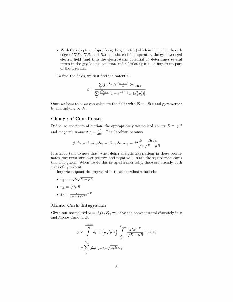
We have defined the probabilistic density of markers:

p(E|µj) ≡Ae−E√E − µjB

Below are illustrations of how this distribtion of markers appears at differentmagnetic field strengths.

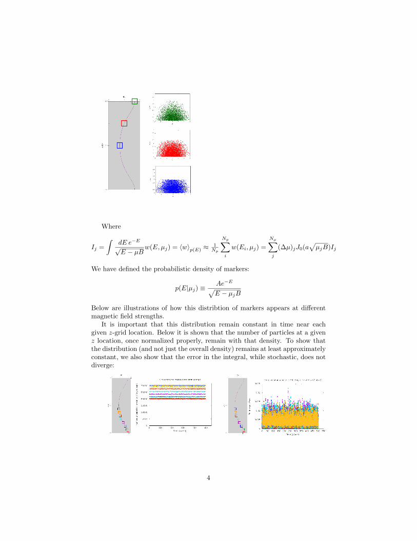
It is important that this distribution remain constant in time near eachgiven z-grid location. Below it is shown that the number of particles at a givenz location, once normalized properly, remain with that density. To show thatthe distribution (and not just the overall density) remains at least approximatelyconstant, we also show that the error in the integral, while stochastic, does notdiverge:

4

The Collision Operator

To calculate the effect of the collision operator, we switch over to using thedistribution function h = 〈φ〉F0 + g to comply with the literature.

We apply Godunov splitting to the gyrokinetic equation so that all the termsbesides C[h] are evaluated explicitly, after which the effect of the collision op-erator (a mixture of diffusion and integral terms) is calculated implicitly. LetA[h] represent the explicit part of the gyrokinetic equation, such that:

dh

dt= A[h] + C[h]

Applying a finite difference scheme in time, we arrive at the pre-collision distri-bution:

h∗ = hn + ∆tA[hn]

And use this to obtain the distributon after a full timestep:

hn+1 = h∗ + ∆tC[hn+1]

Since C[h] contains integral terms, it ought to be considered as a non-sparsematrix. However, as in the code GS2, we apply the Sherman-Morrison methodthat allows us to use one or two tridiagonal matrices (the ones used for the dif-fusive part of the operator) to properly invert the integral terms. See AppendixB of [Barnes, 2009] for details.

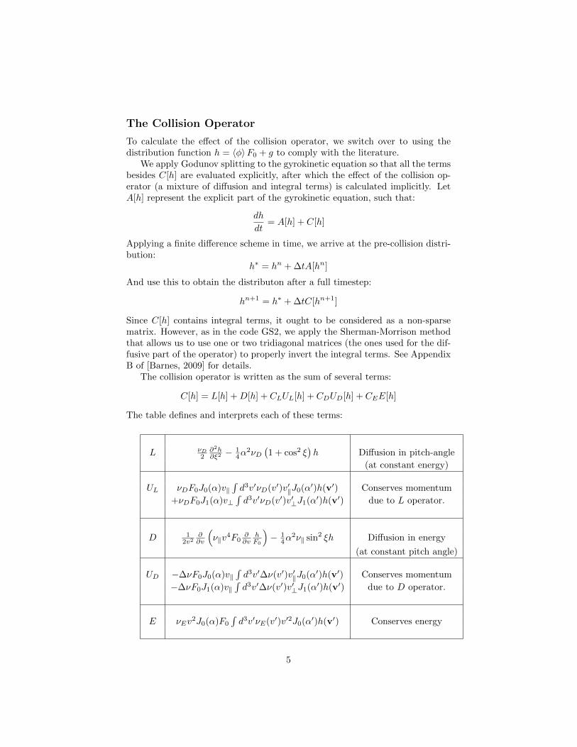
The collision operator is written as the sum of several terms:

C[h] = L[h] +D[h] + CLUL[h] + CDUD[h] + CEE[h]

The table defines and interprets each of these terms:

L νD2∂2h∂ξ2 −

14α

2νD(1 + cos2 ξ

)h Diffusion in pitch-angle

(at constant energy)

UL νDF0J0(α)v‖∫d3v′νD(v′)v′‖J0(α′)h(v′) Conserves momentum

+νDF0J1(α)v⊥∫d3v′νD(v′)v′⊥J1(α′)h(v′) due to L operator.

D 12v2

∂∂v

(ν‖v

4F0∂∂v

hF0

)− 1

4α2ν‖ sin2 ξh Diffusion in energy

(at constant pitch angle)

UD −∆νF0J0(α)v‖∫d3v′∆ν(v′)v′‖J0(α′)h(v′) Conserves momentum

−∆νF0J1(α)v‖∫d3v′∆ν(v′)v′⊥J1(α′)h(v′) due to D operator.

E νEv2J0(α)F0

∫d3v′νE(v′)v′2J0(α′)h(v′) Conserves energy

5

The different νs here are various functions of speed v, to be interpreted ascollision frequencies, and α = k⊥v⊥

Ω . The constants CL, CD, and CE can becomputed ahead of time, and are just integrals over velocity space independentof h.

This collision operator is artificial: it is not derived from first principles butit does satisfy important physical conservation laws as well as the BoltzmannH-theorem. All of these are shown by integrating the collision operator overvelocity space. The zeroth, first, and second moments of the collison operatorvanish by design (note that the integrand and the outside factor of each of theseterms have a similar form; integration by parts along with special definitions ofνD, ν‖, νE and ∆ν are required).

All terms, including inter-species collision terms between electrons and ions,are included in the upgraded GSP. This part of the code still requires validation,especially the conservation options.

3 Implementation

Our approach is the Particle-in-Cell technique: a hybrid Eulerlian/Lagrangianscheme. A pure Lagrangian approach would require the fields be superimposedfrom every particle onto every particle (requiring O(N2

part) operations). Instead,particles are locally deposited onto a grid; the relevant quantities are calculatedon that grid; then reinterpolated back to the particles who then time-advance.This is computationally advantageous if Npart Ngrid, which makes the gridoperations cheap and requiring only O(Npart) + O(Ngrid logNgrid) operations(the Ngrid logNgrid comes from the Fourier transform required to accuratelycompute the gyroaverage.

The particles are each assigned a random position, a random E drawn froma continuous distribution (see Appendix E), one of several discrete values of µ,and a “weight” w. This weight is simply the normalized version of the function

we are solving for: w ≡ 〈δf〉F0. It is initialized randomly, but is advanced in time

according to the ODE along characteristic curves (the right-hand-side of thegyrokinetic equation).

The time-stepping algorithm for the particle weights is a second-order RungeKutta ”predictor/corrector” method:

1. Initialize particles in phase space

2. Predictor step

• Calculate fields at step n

• Calculate marker weights along characteristics for step n+1 /2

• Advance marker positions for half timestep

• Update weights with collision operator for step n+1 /2

3. Corrector step

6

• Calculate fields at step n+1 /2

• Calculate marker weights along characteristics for step n+ 1

• Advance marker positions for the full timestep

• Update weights with collision operator for step n+ 1

4. Output results as necessary

• Repeat steps 2 to 4 as necessary.

Further details on the algorithm are in Appendices C and D.

4 Databases

• GSP Source code (includes relevant revision history under branches/gwilkieand branches/df):http://gyrokinetics.svn.sourceforge.net/viewvc/gyrokinetics/gsp/bran ches/df

– Important sections of code (lines):

∗ Main body, particle orbits: (429-609)

∗ Calculating Phi: (931-1119)

∗ Calculating Fields: (1237-1364)

∗ Updating the weights: (1366-1424)

∗ Collision operator: (1457-2883)

• Original GSP source codehttp://gyrokinetics.svn.sourceforge.net/viewvc/gyrokinetics/gsp/trunk/

• Article with analytic result:

– Ricci, et al, “Gyrokinetic linear theory of the entropy mode in a Zpinch.” Physics of Plasmas, 13: 062102

• Data files included in attached tarball.

5 Validation

We need to ensure that the changes we have made to GSP do not affect itsaccuracy, especially in regimes in which it was originally accurate. We performedthis in two stages: a local validation of the φ integral, and a global validationof the code overall, including particle orbits and time-dependence.

7

Validation of Phi

Since it is such a key part of the algorithm, we validate the φ integral separately.We are validating both the Monte Carlo integration over E and the discretemidpoint rule of µ. To so, we give the function w(E,µ) an artificial value suchthat we know the value of the integral analytically. We have used the followingthree functions:

1. w = 1→ φ ∝ e−k2⊥/2

2. w = E → φ ∝ 12

(3− k2

⊥)e−k

2⊥/2

3. w = sin(2π√E − µB)→ φ ∝ D+(π)e−k

2⊥/2

Where D+ is the Dawson integral. The latter function is most indicative of thekinds of perturbations that are seen, and have the added advantage of havingsome structure in velocity space and depends on both E and µ.

Each of these integrals is performed for many different combinations of kx

and ky (where the result depends only on k⊥ =√k2x + k2

y), and the numerical

result is compared with the known analytic function, given in green. We alsoplot the logarithmic scale of these graphs to the right to more clearly show thedifferences as a function of k⊥.

8

Upon more careful examination, it is realized that the error is stochasticand simply changing the random number seed will result in a different error.Below is an example of several different resolutions, each run 40 times each withdifferent seeds.

And finally, to make it clear that the error that we see is from the MonteCarlo integration (and is thus remedied by adding more particles), we calculatethe integral 40 times for many different numbers of particles per cell (there are1024 cells to generate the appropriate resolution of k⊥ shown agove).

9

Physical Validation: Z-pinch Entropy Mode

Here, we combine the calculation of the fields along with particle trajectoriessubject to curvature and gradient drifts. The geometry of the problem is showbelow:

The gradient of the magnetic field and the plasma density is toward the cen-ter (−x). Such a configuration gives rise to an instability along the y-directionwhose dispersion relation is known (see [Ricci, 2006]). We compare our code toanother, more established code GS2. This code is purely Eulerian and solvesthe gyrokinetic equations fully implicitly.

To study the growth rates, we look at the growth of the following function:

Φ(ky) =∑kx,kz

|φ(kx, ky, kz)|2

This is a measure of how much electrostatic energy is in a particular ky mode.Its growth rate is found by solving the finite difference formula for exponentialgrowth:

Φn+1 − Φn

∆t= γ

(Φn+1 + Φn

2

)Where the superscript denotes the time step, and γ is the growth rate. Thisquantity is updated as an exponentially-weighted moving average so that theoutput is easily read. Alternatively, one could simply estimate the slope of alogarithmic chart of such growth.

According to the dispersion relation, different ky modes are going to havedifferent growth rates. Here, we compare to this growth rate spectrum to theGS2 prediction for a variety of test conditions. Let Ln be the density gradientlength scale (such that ∇nn = 1

Ln); similarly for the temprature scale LT ; R is

the radius of curvature; and Ti and Te are the ion and electron temperatures,respectively.

1. Standard Case: LnR = 0.5, R = 1, Te = Ti = 1, 1

LT= 0

2. High n Gradient Case: Same as standard with LnR = 2.0

10

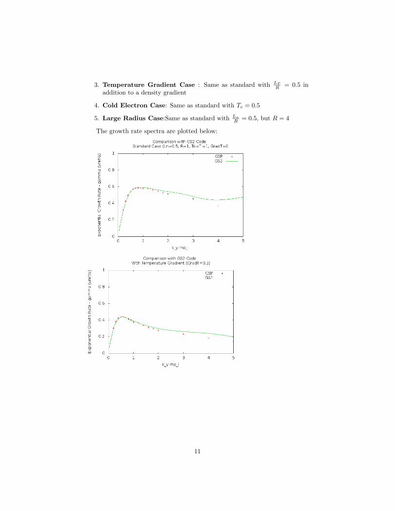
3. Temperature Gradient Case : Same as standard with LTR = 0.5 in

addition to a density gradient

4. Cold Electron Case: Same as standard with Te = 0.5

5. Large Radius Case:Same as standard with LnR = 0.5, but R = 4

The growth rate spectra are plotted below:

11

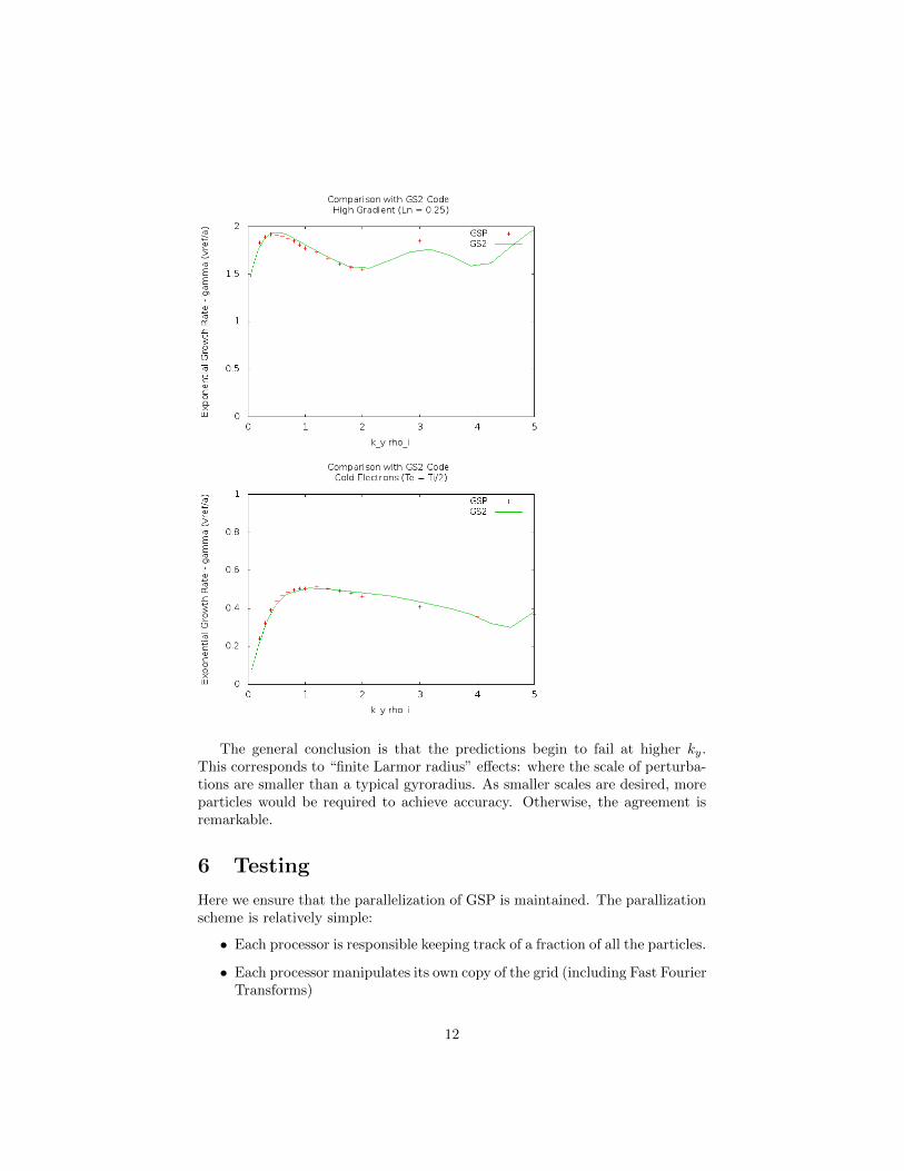
The general conclusion is that the predictions begin to fail at higher ky.This corresponds to “finite Larmor radius” effects: where the scale of perturba-tions are smaller than a typical gyroradius. As smaller scales are desired, moreparticles would be required to achieve accuracy. Otherwise, the agreement isremarkable.

6 Testing

Here we ensure that the parallelization of GSP is maintained. The parallizationscheme is relatively simple:

• Each processor is responsible keeping track of a fraction of all the particles.

• Each processor manipulates its own copy of the grid (including Fast FourierTransforms)

12

– The exception is the collision operator. Since the grid there is in 5Dphase, space, it makes sense to split these among the processors.

• The only communication among processors is when the grid is calculated.A sum allreduce operation is performed which adds the contribution fromall the particles on each of the processors.

We perform the following scaling tests:

• Weak scaling: Increase the number of processors in proportion to theproblem size. (1 to 192 cores)

• Strong scaling: Increase the number processors for fixed problem size.(1 to 960 cores)

The former is just as important: it means that we can always add more proces-sors to reduce noise. We do not expect this parallelization scheme to work whenthe number of particles per processor approaches the number of grid points. Wehave added an expensive per-particle operation (the sqrt necessary to find v‖)that may cause scaling to become poor well before this point.

These tests were run on Hopper, a NSERC supercomputer, utilizing up to960 cores. For these cases, Npart.percell = 1600 and Ngrid = 256, giving 400kparticles total. Therefore, we would not expect the problem to scale well asNproc → 1600.

The quantities plotted should be constant for perfect scaling. We find thatthe algorithm scales well weakly, but is sensitive to strong scaling. The inclusionof the sqrt operation is likely to blame for this decrease in performance at highnumbers of processors.

13

14

7 Schedule and Milestones

Phase I: AnalyticsSeptember - December 2011

• Understand rigorous derivation of the gyrokinetic equation• Become familiar with analytical aspects of the gyrokinetic equation• Make velocity coordinate change• Understand algorithm used by GSP to solve GK equation• Understand Abel collision operator and how it is to be implemented in

GSP• Milestone: Derive GK equation in velocity coordinates E and µ.

Phase II: NumericsDecember 2011 - March 2012

• Become familiar with GSP code• Make proposed changes to the code• Ensure code still runs• Code collision operator• Milestone: GSP Code updated with new velocity coordinates.

Phase III: Testing and ValidationApril 2012

• Debug updated GSP code• Validate and test against previous version and known results• Run test cases, organize results• Milestone: GSP code in new velocity coordinates validated and tested

Phase IV: CommunicationMay 2012

• Prepare final presentation• Milestone: Final presentation given

8 Deliverables

• Updated GSP source code• Sample input file and instructions• Test case comparison data• Final presentation• Final Report

15

9 Bibliography

• Abel, et al. “Linearized model Fokker-Planck collision operators for gy-rokinetic simulations. 1. Theory.” Physics of Plasmas, 15:122509 (2008)

• Antonsen and Lane, “Kinetic equations for low frequency instabilities ininhomogeneous plasmas.” Physics of Fluids, 23:1205 (1980)

• Aydemir, “A unified Monte Carlo interpretation of particle simulationsand applications to non-neutral plasmas.” Physics of Plasmas, 1:822(1994)

• Barnes, et al. “Linearized model Fokker-Planck collision operators for gy-rokinetic simulations. 2. Numerical Implementation and Tests.” Physicsof Plasmas, 16:072107 (2009)

• Barnes, “Trinity: A Unified Treatment of Turbulence, Transport, andHeating in Magnetized Plasmas.” PhD Thesis, University of MarylandDepartment of Physics (2009)

• Broemstrup, “Advanced Lagrangian Simulations Algorithms for Magne-tized Plasma Turbulence.” PhD Thesis, University of Maryland Depart-ment of Physics (2008)

• Catto, “Linearized gyro-kinetics.” Plasma Physics, 20:719 (1978)

• Dimits, et al, “Comparisons and physics basis of tokamak transport mod-els and turbulence simulations.” Physics of Plasmas, 7: 969 (2000)

• Frieman and Chen, “Nonlinear gyrokinetic equations for low-frequencyelectromagnetic waves in general plasma equilibria.” Physics of Fluids,25:502 (1982)

• Howes, et al. “Astrophysical gyrokinetics: basic equations and lineartheory.” The Astrophysical Journal, 651: 590 (2006)

• Ricci, et al, “Gyrokinetic linear theory of the entropy mode in a Z pinch.”Physics of Plasmas, 13: 062102 (2006)

Appendix A: Gyroaveraging

Often, quantities will need to be ”gyroaveraged” over a circle determined by theparticles’ velocity and the local magnetic field. This operation is defined by:

〈A(r)〉R ≡∫dθ A(R + ρ(θ))

Where 〈A(r)〉R means the ”gyroaverage of A at fixed gyrocenter R”. Likewise,we have:

〈A(R)〉r ≡∫dθ A(r− ρ(θ))

In Fourier space, we find that the gyroaverage operation becomes a Bessel func-tion factor:

〈a(kr)〉R = J0

(k⊥v⊥

Ω

)a(kR)

16

Appendix B: Poisson’s Equation

The fields above are found by applying Poisson’s equation, which to this orderis the condition of quasineutrality :∑

s

δnsqs = 0

Where the sum is over all species (typically ions and electrons). The perturbeddensity δn is the moment of the distribution function:

δn =

∫d3v 〈δf〉r

Where we acknowledge that the charges form rings and we need to averageat constant position in space and not at constant gyrocenter since particlesof different gyrocenters will contribute to the charge at a particular point inspace. Since the function h (which we eliminate in our formulism) is already agyroaveraged quantity: 〈h〉R = h, we can write:

δf + φF0 = 〈δf〉R + 〈φ〉R F0

Therefore:〈δf〉r = 〈〈δf〉R〉r + F0 〈(〈φ〉R − φ)〉r

In Fourier space, the sum over species in Poisson’s equation looks like:∑s

qs

∫J0 〈δf〉R d

3v + φn0,s

(2π)3/2

∫e−

12v

2

(J0 − 1) d3v

Rearranging and applying an integral identity for I0:

φ =

∑s

∫d3vJ0 〈δf〉R,s∑

s

q2sn0,s

Ts

[1− e−k2⊥ρ2sI0 (k2

⊥ρ2s)]

Appendix C: Algorithm for Calculating the Fields

We summarize here how the fields are found given 〈δf〉:

1. For each species:

• For each µi:

(a) Use bilinear interpolation to find 〈δf〉 on a grid in R-space.

(b) In the processes of depositing the particles onto the grid, performthe Monte Carlo integration over the velocity space variable E

(c) Fourier transform in X and Y

(d) Multiply by J0 (stored in memory) and normalize

17

• Integrate discretely over µ (mid-point rule)

2. Sum over species to find φ

3. Fourier transform over Z

4. Calculate 〈E〉R = −ikJ0φ

5. Inverse Fourier transform in 3D

6. Reinterpolate so that the field is known at each particles’ position.

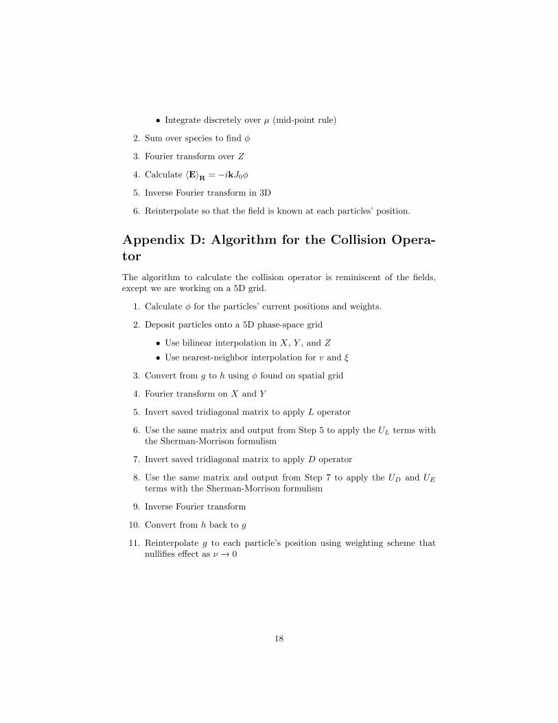
Appendix D: Algorithm for the Collision Opera-tor

The algorithm to calculate the collision operator is reminiscent of the fields,except we are working on a 5D grid.

1. Calculate φ for the particles’ current positions and weights.

2. Deposit particles onto a 5D phase-space grid

• Use bilinear interpolation in X, Y , and Z

• Use nearest-neighbor interpolation for v and ξ

3. Convert from g to h using φ found on spatial grid

4. Fourier transform on X and Y

5. Invert saved tridiagonal matrix to apply L operator

6. Use the same matrix and output from Step 5 to apply the UL terms withthe Sherman-Morrison formulism

7. Invert saved tridiagonal matrix to apply D operator

8. Use the same matrix and output from Step 7 to apply the UD and UEterms with the Sherman-Morrison formulism

9. Inverse Fourier transform

10. Convert from h back to g

11. Reinterpolate g to each particle’s position using weighting scheme thatnullifies effect as ν → 0

18

Appendix E: Normalization and Generation ofthe Monte Carlo Probability Distribution

We have defined p(E) = A e−E√E−µB . Since

Emax∫µB

p(E)dE = 1 necessarily, we find

the normalization constant:

1

A= e−µBErf

(√Emax − µB

)Furthermore, in order to obtain this distribution from a standard [0,1] uni-

form random distribution, we need to invert the cumulative distribution:

y = P (x) = A

x∫µB

dEe−E√E − µB

To obtain:

x = µB +(

Erf−1[yErf

(√Emax − µB

)])2

Appendix F: Quasirandom Sequence Monte CarloImprovement

It was discovered that we can get better than the typical 1√N

error dependence

from Monte Carlo by uniformly filling the integration domain with particlesdistributed according to a quasirandom sequence rather than pseudorandomor truly random placement. This avoids errors that result from a spuriousdistribution that would occur by chance.

While the implementation appears to be imperfect, the decrease in error isworth note.

19