Amplitude-Probability Distributions for Atmospheric Radio .../67531/metadc13201/m2/1/high... ·...

NBS MONOGRAPH 23

Amplitude-Probability Distributions for Atmospheric Radio Noise

U.S. DEPARTMENT OF COMMERCE

NATIONAL BUREAU OF STANDARDS

THE NATIONAL BUREAU OF STANDARDS

Functions and ActivitiesThe functions of the National Bureau of Standards are set forth in the Act of Congress, March

3, 1901, as amended by Congress in Public Law 619, 19SO. These include the development and maintenance of the national standards of measurement and the provision of means and methods for making measurements consistent with these standards; the determination of physical constants and properties of materials; the development of methods and instruments for testing materials, devices, and structures; advisory services to government agencies on scientific and technical problems; inven tion and development of devices to serve special needs of the Government; and the development of standard practices, codes, and specifications. The work includes basic and applied research, develop ment, engineering, instrumentation, testing, evaluation, calibration services, and various consultation and information services. Research projects are also performed for other government agencies when the work relates to and supplements the basic program of the Bureau or when the Bureau's unique competence is required. The scope of activities is suggested by the listing of divisions and sections on the inside of the back cover.

PublicationsThe results of the Bureau's work take the form of either actual equipment and devices or pub

lished papers. These papers appear either in the Bureau's own series of publications or in the journals of professional and scientific societies. The Bureau itself published three periodicals available from the Government Printing Office: The Journal of Research, published in four separate sections, presents complete scientific and technical papers; the Technical News Bulletin presents summary and preliminary reports on work in progress; and Basic Radio Propagation Predictions provides data for determining the best frequencies to use for radio communications throughout the world. There are also five series of nonperiodical publications: Monographs, Applied Mathematics Series, Handbooks, Miscellaneous Publications, and Technical Notes.

Information on the Bureau's publications can be found in NBS Circular 460, Publications of the National Bureau of Standards ($1.25) and its Supplement ($1.50), available from the Super intendent of Documents, Government Printing Office, Washington 25, D.C.

UNITED STATES DEPARTMENT OF COMMERCE Frederick H. Mueller, Secretary

NATIONAL BUREAU OF STANDARDS A. V. Astin, Director


W. Q. Crichlow, A. D. Spaulding, C. J. Roubique, and R. T. Disney

National Bureau of Standards Monograph 23

Issued November 4, 1960

For «al« by the Superintendent of Document*, U.S. Government Printing Office, Washington 25, D.C. - Price 20 cent*

ContentsPage

1. Introduction ___________________________________________ 12. References._________________________________________________ 23. Appendix, __________________________________________________ 15

1. Introduction________________________________ 152. Measurements of the amplitude-probability distribution. ________ 153. Definition of parameters and statistical moments.______________ 164. Determination of the parameters as functions of the measured

moments. ______________________________________________ 175. Errors in noise measurements and their influence on the calculated

distribution, _____________ _____________.___________ 186. Bandwidth considerations. __________________________________ 207. References. _______________________________________________ 22

ii


W. Q. Crichlow, Q. D. Spaulding, C. J. Roubique, and R. T. Disney

Families of amplitude-probability distribution curves are presented in a form such that by using three statistical parameters of atmospheric radio noise, of the type published by the National Bureau of Standards, the corresponding amplitude-probability distribution may be readily chosen. Typical values of these parameters are given.

1. Introduction

A knowledge of the detailed characteristics of atmospheric radio noise is essential to the design of radio communication systems operating at frequen cies up to about 30 Mc/s. These characteristics can conveniently be expressed in terms of an amplitude- probability distribution which has been found to be an extremely useful tool in the analysis of the expected interference to a communication system [I]. 1 However, since the measurement of the complete amplitude-probability distribution on a continuous basis for many frequencies and locations is pro hibitive in both manpower and equipment needs, a method of obtaining this distribution from three easily measured statistical moments has been de veloped at the National Bureau of Standards [2]. The three moments are the average power, the average envelope voltage, and the average logarithm of the envelope voltage, and are expressed, respec tively, as:

Fa=the effective antenna noise figure,=the external noise power available from an

equivalent, short, lossless, vertical antenna in decibels above ktb (the thermal noise power in a passive resistance at room temperature, f, in a bandwidth, 6),

Frf=the ̂ voltage deviation in decibels below Fa , L d=the log deviation in decibels below Fa -

Fa can be expressed in terms of the root mean square field strength by means of the nomogram in figure 1. It should be noted that although Fa is independent of bandwidth, the root mean square field strength is proportional to the square root of the bandwidth used.

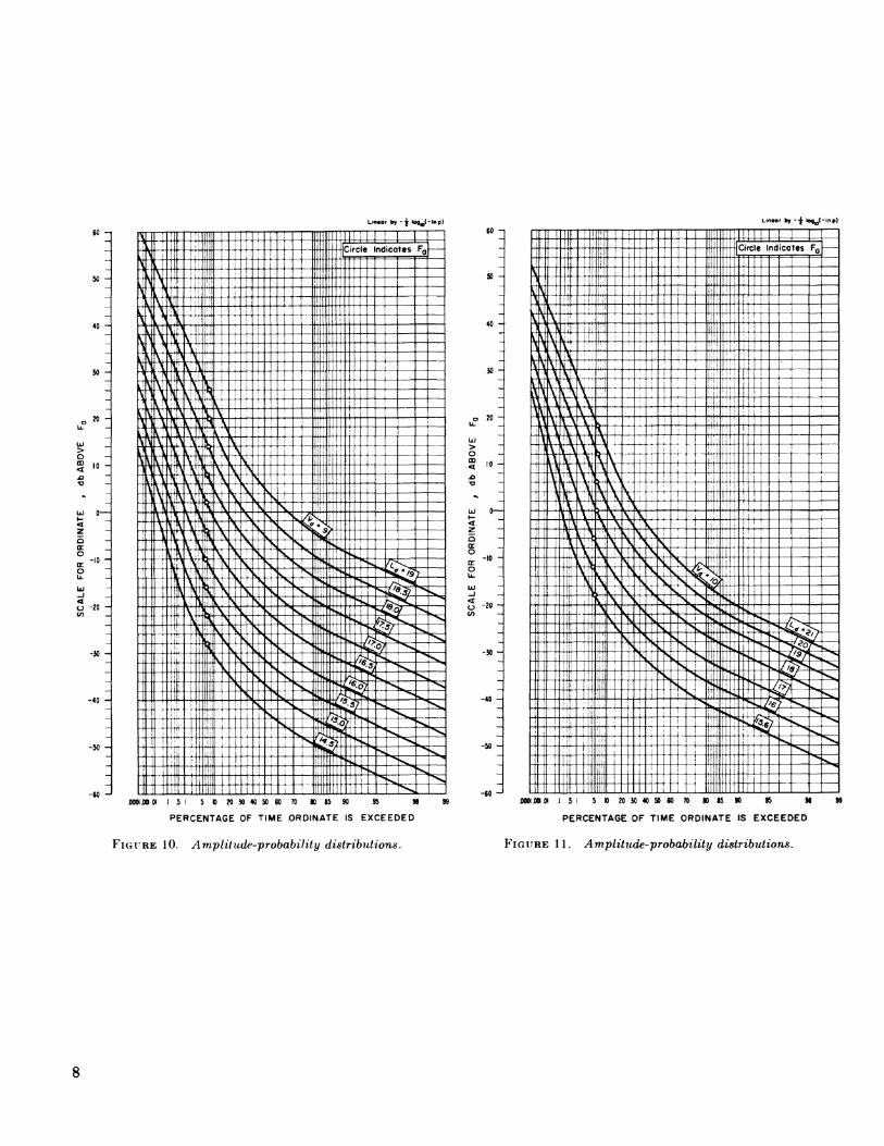
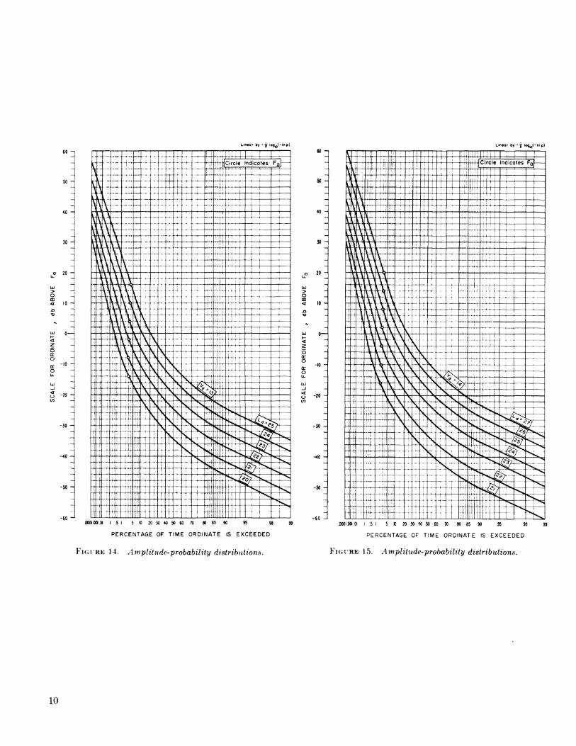
The shape of the distribution curve is dependent only on Vd and Ldj and since they have been nor malized to Fa , it is possible to construct [2] distribu tion curves for various combinations of these param eters, independently of the value of Fa . Such curves are given in figures 2 through 21 for the range of values of Vd and Ld for which the distribution is valid. These curves give the percentage of time

1 Figures in brackets indicate the literature references on page 2.

the ordinate is exceeded. In order to minimize the number of graphs required, several curves have been drawn on each graph at arbitrary levels. The circle on each curve corresponds to the value of Fa (the root mean square voltage for the distribution) and by shifting the ordinate scale so that zero decibel corresponds to the circle on the proper curve, the ordinate can be determined in decibels above Fa .

Values of Fa , Vd , and Ld are recorded continuouslv at ten of the stations in the worldwide network established by NBS [3]. These recordings are made at eight fixed frequencies between 13 kc/s and 20 Mc/s, using a bandwidth of about 200 c/s, and the data are published [4, 5] in tabular form. Values of Fa only are recorded at six additional stations in the network and are included in the publications. In addition, predictions of worldwide values of Fa have been published by C.C.I.R. [6].

Typical values of the three parameters are shown in figures 22 and 23. Figure 22 gives Fa versus frequency for summer nighttime and winter day time, which are the periods of highest and lowest atmospheric noise levels, respectively. Curves are shown for the estimated values of Fa for each type of noise (atmospheric, galactic, and manmade) by taking into account propagation conditions as well as the recorded values.

Figure 23 gives Vd and Ld versus frequency for summer nighttime and winter daytime. The curves were not drawn through all of the measured points, since some signal contamination has been encoun tered and the smoothed curves are considered more representative of true conditions. The portions of the Vd and Ld curves that result from each of the three noise sources will be the same as shown for Fa in figure 22.

Although the distribution curves given in figures 2 through 21 are considered valid for a wide range of bandwidths, the values of Vd and Ld used in de termining the distribution must correspond to the bandwidth to be used. The values given in figure 23 are for a 200 c/s bandwidth and must be adjusted for any other bandwidth. Methods of converting these statistical moments from one bandwidth to another are under development at NBS and will be published in the near future.

2 References ical Year July ^ 1957-December 31, 1958, NBS Tech.*,. AWWX^HWOD Note ^ (pB 151377) (Jujy 27j jg^

n Watt R M Toon F L Maxwell and R W Plush I 4 ' W ' Q- Crichlow> c - A Samson, R. T. Disney, and M. A. -

thermal and atmospheric noise, Proc. IRE 46, 12, 1914 (March 14 1960)

[2] W. Q. Crichlow, C. J. Roubique, A. D. Spauldirig, and (51 w - Q- Crichlow, Noise investigation at VLF by theW. M. Beery, Deter mination of the amphtude-probabil- National Bureau of Standards, Proc. IRE 45, 6, 778ity distribution of atmospheric radio noise from statis- (1957).tical moments, J. Research NBS 64D, 49 (1960). (See [6] Report on Revision of Atmospheric Radio Noise Data,appendix.) C.C.I.R. Rept. No. 65, VHIth Plenary Assembly, War-

13] W. Q. Crichlow, C. A. Samson, R. T. Disney, and M. A. saw (Intern. Radio Consultative Comm., Secretariat,Jenkins, Radio noise data for the International Geophys- Geneva, Switzerland) (1956).

W/s (Megacycles)"i:

- rTO60- i--hso

20-^-

0090.07

0.05-i-

0.03 Hh

0.01 -1-

--2

-hO.7 0.6-^

-hO.5 04- -

-j-0.3

02--

-0.1 : OJ08 006

--0:02

F( (db obo

"

o-

40-

80-

120-

160-

3 (db abov< ve ktb)

--20 ;-40-

__ —

^ -

-20 : -20-

-

0- -60

20-

-100

40-

-140

60-

—

-1808fl-

1 1 2 1 ^

—50

--30

--10

-10

-30

-50

_

-70

20log 10 fMc/r 65.5

FIGURE 1. Nomogram for transforming effective antenna noise figure to noise field strength as a function offrequency.

Fa effective antenna noise figure=external noise power available from an equivalent short, lossless, vertical antenna in decibels above ktb. J?n=equivalent vertically polarized ground-wave root mean square noise field strength in decibels above 1 /iv/m fora 1-kc/s bandwidth, fuel*** frequency in megacycles.

Liiwor br -| lofl^t-lnp)

g

? ,0

o cc o

I5I5I0203040S06070W8590 95 98 99

PERCENTAGE OF TIME ORDINATE IS EXCEEDED

0001,00(01 J 5 I 5 » 20 30 40 50 $0 70 80 85 90 95 98 99


FIGURE 2. Amplitude-probability distributions. FIGURE 3. Amplitude-probability distributions.

50 -

Os ..

-50 -

-20 -

5 10 20 30 40 50 60 TO 80 85 90 95 98


1 510203040506070608590 95 94



50 -

gCD

z

o

10 -

Lmtor by -£ log^Hnp)

o3

Z Oo: o

-30 -

WWW 01 .131 5 1C 20 50 40 50 $0 70 80 85 90 95


-60 -JDOCH .00 JDI I 5 I 5I0203040S060TO 80 55 90 35 98



50 -

30 -

20 -

o5

Oct oor o

60 -i

0001501.01 .1 5 I 5 tt 20 30 40 50 60 70 W 85 90 95 98 99


FIGURE 8. Amplitude-probability distributions.

30 ^

o 20 -

10 -

0o: o or o

LU_l

S -20V)

-30 -

JXXHOOICrt 151 5 10 20304

PERCENTAGE OF

' 50 60 TO 90 85 90 95 90

TIME OROINATE IS EXCEEDED


560873 O - 60 - 2

50 -

O

5

UJ

2-H

-50 -

DOOTOQOI 151 5 K) W 30 40 50 80 70 80 »5 90 95 M


I 5 I 5 10 20 JO 40 50 60 70 80 «5 90 95 91 99

PERCENTAGE OF TIME ORDtNATE IS EXCEEDED


o00< 10

o tr oor o u.

O

S n

CK O

-20 -

JOOOtttlOl .15! 5 » ?0 JO 40 50 60 TO *3 85 90 95 96


-50 -

-60 -1000* .W 51 J5l5ft?030405Q6QroaOti90 95 M 99


FIGURE 12. Amplitude-probability distributions. FIGURE 13. A mplitude-probability distributions.

by -^ logw(-lnp)

50 -

30 -

§ 00< 10 •

o a: o

50 -

< 10 -

zQa: oor o

DOOl.IMi.Ot .1 .5 I 5 10 20 30 40 50 60 70 80 85 90 95 98


FiGt'RE 14. A in plit ude- probability distributions.

JDOOI.OOI.OI .1 .5 I 5 K) 20 30 40 50 60 70 80 85 90 95 98



10

50 -

O

3 ,0

Q IT O

_t <

-50 -

iMOf by -•$• logw(-lnp)

o: O

-20 -

J 5 S 10 20 30 40 SO 60 70 M 85 90 95 98



OOOTOOIDi J 5 I 5 10 20 30 40 50 60 70 80 85 90 95 9«


FIGIBE 17. Amplitude-probability distributions.

11

o cr ocr - |0 oU.

LJ_J

o -20 en

-50 -

30 -

o5 »•

Otr otrs

DOOUOOI.OI .151 5102030405060 TO 808590 95 98

PERCENTAGE OF HME ORDINATE IS EXCEEDED

FIOTRE 18. Amplitude-probability distributions.

-30 -

-50 -

-60 -10001001.01 I .5 I 5 D 20 30 40 50 60 70 90 85 90 95 W



12

50 -1

O

3 ,«

UJ

6Otr occ. o

-10 -

-30 -

-50 -

DOOtOatt J5I5B20304C50S07080S590 95 96 99



IJWJ5I5I020304050WT080S590 95 98 99

PERCENTAGE OF TIME ORDINATE !S EXCEEDED


13

190

180

170

160

150

140

130

120

110

IOO

90

80

70

60

50

4O

30

20

10

0

, . , , ,

————— ..... .

v»^v

*-.—— ,.+ ,. .;.,-. *._.!..... i| . ... ...,.:«X) —— 0- MEDIAN SUMMER NIGHTTIME (20 -24 hr) — Q —— O— MEDIAN WINTER DAYTIME (08 - 12 hr)

I RANGE BETWEEN UPPER AND LOWER DECILE

^>^^

"••- ••--• -«sDL

^\ -— * :V

1— : V--\

' Xs

j,.,~.

!^_.

."S*^

j i 1 1 ' -Wtfff/C

( !

1

J — -- --•f^ I.. ., -. ^

^Njl 'Ysi x ^ ,

IA,T ^ t*^1 iiIVVk. Tx^\ * "v%vli

——A T^ |\ T ^">-\ — ̂ ^

. , \ . _ I\ i\ i i\ M>! \

\Pto '

i 'l 't\

f

^s.

>„_ -.^Vi

JL*\XJ

y*\

^X^ T X;^^XOL i^^sL^Xs5

jjJrj

, i , , / ,' ' ' y

X >f^•^-4— ̂ '• ;

.

\ " '\ ' ^

rALACTiC J ——

^kJ 1t^vx^ iJil^s\^**S'4Lt t'Y"!"" n

0.01 0.02 0.05 O.I 0.2 O.5 I 2 5 IO 20

FREQUENCY IN MEGACYCLES

FIGURE 22. Radio noise levels measured during ICY, dun- barrel Hill, Boulder, Colo.

O.t I 10

f Mc/S (a) Summer Nighttime (20-24 hr)

Ld HIT

T Mc/s (b) Winter Daytime (08 - 12 hr)

FIGrRE 23. Radio noise statistical parameters.

Measured during summer 1959 and winter 1958-1959, Ounbarrel Hill, Boulder,Colo.

14

3. Appendix

Determination of the Amplitude-Probability Distribution of Atmospheric Radio Noise From Statistical Moments *

W. Q. Crichlow, C. J. Roubique, A. D. Spaulding, and W. M. Beery(July 23, 1959)

During the International Geophysical Year, the National Bureau of Standards estab lished a network of atmospheric noise recording stations throughout the world. The ARN-2 noise recorder at these stations measures three statistical moments of the noise: average power, average voltage, and average logarithm of the voltage. An empirically-derived graphical method of obtaining an amplitude-probability distribution from these three moments, and its development, is presented. Possible errors, and their magnitudes, are discussed.

1. Introduction

The interference to reception of radio signals caused by atmospheric noise depends not only on its average level but also on its detailed characteris tics. A complete description of the noise received at a particular location would require an exact determination of the variation of its instantaneous amplitude as a function of time. Because of the complexity of the noise structure and the fact that no two samples of noise have identical amplitude- time functions, it is necessary to resort to simpler types of description of a statistical nature.

Various methods of measurement have been in vestigated by experimenters throughout the world for many years, and the relationship between the measured values and the interference caused to various types of service has been studied.

In order to determine the most significant charac teristics to be measured, an international subcom mittee was formed within Commission IV of UKSI l to study the problem. A recommendation [I],1 based on the subcommittee's report [2], was endorsed by Commission IV at the Xllth General Assembly of the URSI in 1957. In the Annex to this recommenda tion, it is stated that "it would be highly desirable to obtain detailed statistical information on the ampli tude-probability distribution of the instantaneous envelope voltage, the various time functions, and the direction of,arrival of the noise at many locations throughout the world. However, since continuous detailed measurements of this type at all frequencies and a large number of stations become prohibitive because of the complexity of the equipment involved and the large number of personnel necessary to carry out the observations, it is recommended that these complete studies of the detailed noise characteristics be confined to a few selected locations with continuous measurements of one or more simple parameters at a large number of stations/'

•Reprinted from J, Research NBS, Vol. 64D, No. 1, Jan.-Feb. 1960.* International Scientific Radio Union.' Figures in brackets indicate the literature references at the end of this paper.

During the International Geophysical Year, the National Bureau of Standards established a network of 16 noise recording stations distributed throughout the world [3]. Measurements are made witn the ARN-2 recorder which was designed at NBS to record the average noise power in a bandwidth of about 200 cps on eight fixed frequencies between 13 kc and 20 Me. In order to obtain additional information on the character of the noise, two other statistical moments, the average envelope voltage, and the average logarithm of the envelope voltage are recorded at ten of the stations. These data are available from IGY World Data Center A, NBS, Boulder, Colo., at a nominal fee. The results of data analysis will also be published in an NBS Technical Note for public sale.

The amplitude-probability distribution is very useful in assessing the interference potential of noise and has been measured at several locations [4, 5, 6, 7], Since data on the moments measured by the ARN-2 can be recorded continuously over the full frequency range with much less equipment and fewer personnel than would be required for a comparable amount of data on the complete amplitude-probability distribu tion, an investigation was made at the NBS of methods of deriving the complete distribution from these three moments.

It is the opinion of the authors that mathematical models for the distribution [1,5,7,8] have proved to be extremely cumbersome and of doubtful value in deriving the distribution from measured moments; therefore, an empirically derived graphical method has been developed.

2. Measurements of the Amplitude- Probability Distribution

Simultaneous measurements of the amplitude- probability distribution and the three moments measured by the ARN-2 were needed over a wide frequency range with a variety of types of noise. There were two specific purposes in making these measurements:

15

a. The distribution measurements, alone, were needed to establish typical shapes that could be ex pressed by numerical parameters, easily related to the measured statistical moments.

b. The simultaneous measurements of the distri butions and the moments were needed to check the accuracy of the ARN-2 noise recorder in measuring the moments.

Accordingly, a distribution meter was constructed to be used in conjunction with the ARN-2 recorder.

The operation of the distribution meter is based on counting techniques. The total number of IF cycles in the ARN-2 which exceed a specified ampli tude in a given time interval are counted. By proper choice of the time interval, the percentage of time a level is exceeded can be read directly from the counter. Three counters are used to provide simul taneous measurement at three levels, separated in amplitude by 6 db. By use of a calibrated, man ually-operated attenuator, the total possible range of 100 db can be covered in levels separated by multiples of 2 db. The time duration of each sam ple can be preset to provide an automatically timed sample having an interval ranging from 1 sec to 1 hr, in 1 sec increments.

The actual intervals were chosen of sufficient dura tion to provide a statistically significant sample of a slowly varying phenomenon such as thunderstorm activity. Longer intervals were required for the high-level, low-probability noise pulses than for the low-level, high-probability noise. The time neces sary to obtain a complete curve ranged from about 15 min to 30 min. The longer period was necessary for measuring noise with a large dynamic range.

A check for accuracy of operation was made by obtaining a distribution of thermal noise. The Rayleigh distribution thus obtained confirmed the accuracy of measurement. Figure 1 is a typical amplitude-probability distribution of atmospheric radio noise at 13.3 kc. This was plotted on Rayleigh graph paper, whose coordinates were chosen so that a Rayleigh distribution will plot as a straight line with a slope of — }{? The coordinates are shown as noise level in decibels above the root mean square voltage versus the percentage of the time that each level is exceeded. This measurement was made with the distribution meter at the Boulder Labora tories. The dynamic range between the 0.0001 per cent and 99 percent intercepts is approximately 84 db.

It was found that these amplitude-probability distributions for atmospheric radio noise can be ade quately represented by a three-section curve which has been drawn through the data points in figure 1. This curve has a characteristic shape that can be described by means of four numerical parameters to be defined later. The accuracy of fit using this par ticular kind of curve composed of three sections is typical of more than 100 distributions experimentally measured at Boulder. In the particular case of thermal noise, this curve becomes a straight line.

« These coordinates are logo! voltage versus—M logio (—In of probability).

10 LJJ

-10

-20

-30

\\\

Frequency - 13.3 kc1537 October 6, 1958

Boulder, Colorado

-40 00001OJOI 0.1 I 5 K) 20 30 40 50 60 70 80 90 95 98 99


FIGURE 1. Measured amplitude-probability distribution of atmospheric radio noise.

Data obtained by other experimenters [2] in Alaska, Panama, England, and Florida when plotted on Rayleigh paper also fit curves of this form.

The lower portion of the curve, representing low voltages and high probabilities, is composed of many random overlapping events, each containing only a small portion of the total energy. Therefore, this portion of the curve must approach a Rayleigb distribution.

The section representing very high voltages ex ceeded with low probabilities is, in general, composed of nonoverlapping large pulses occurring infrequently. From experimental measurements of atmospheric noise distributions, this section has been found to be well represented by a straight line on Rayleigh graph paper. On this graph paper, the remaining section of the distribution has been found to correspond quite closely to an arc of a circle tangent to the above two straight lines. Based on experimental evidence, it is assumed that no pulses of amplitude greater than those for which the probability of being exceeded is 10~6 are present in the distribution.

3. Definition of Parameters and Statistical Moments

Since on the coordinate paper used for the ^^^^^ of amplitude distributions for atmospheric radio noise a Rayleigh distribution will always have a slope of — %, and since the center of the circular arc men-

16

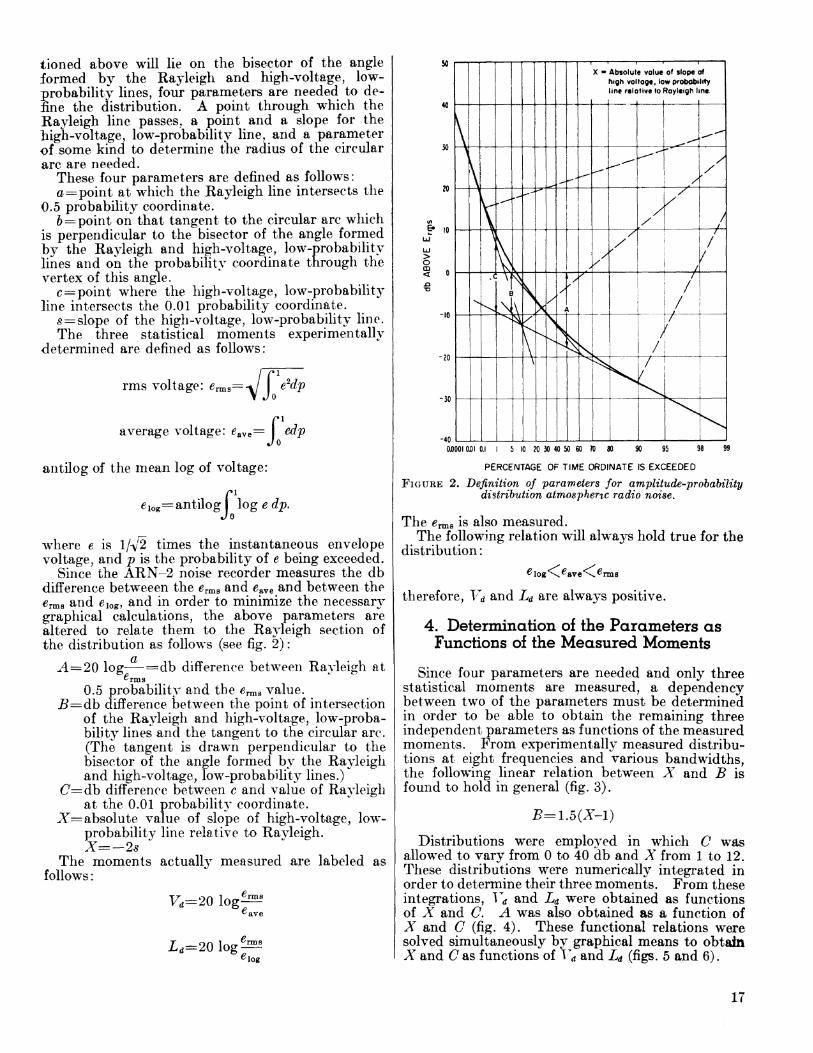
tioned above will lie on the bisector of the angle formed by the Rayleigh and high-voltage, low-

Erobability lines, four parameters are needed to de ne the distribution. A point through which the

Rayleigh line passes, a point and a slope for the high-voltage, low-probability line, and a parameter of some kind to determine the radius of the circular arc are needed.

These four parameters are defined as follows:a =point at which the Rayleigh line intersects the

0.5 probability coordinate.1 = point on that tangent to the circular arc which

is perpendicular to the bisector of the angle formed by the Rayleigh and high-voltage, low-probability lines and on the probability coordinate through the vertex of this angle.

c=point where the high-voltage, low-probability line intersects the 0,01 probability coordinate.

$ =slope of the high-voltage, low-probability line.The three statistical moments experimentally

determined are defined as follows:

rms voltage: e rms=

average voltage: £ave —Jo

antilog of the mean log of voltage:

6i0g=antilog I log e dp. Jo

where e is l/-y2 times the instantaneous envelope voltage, and p is the probability of e being exceeded.

Since the ARN-2 noise recorder measures the db difference betweeen the e Tm3 and £ave and between the erms and 6 log , and in order to minimize the necessary graphical calculations, the above parameters are altered to relate them to the Rayleigh section of the distribution as follows (see fig. 2) :

^4=20 log——=db difference between Rayleigh at0.5 probability and the eTms value.

J3=db difference between the point of intersection of the Rayleigh and high-voltage, low-proba bility lines and the tangent to the circular arc. (The tangent is drawn perpendicular to the bisector of the angle formed by the Rayleigh and high-voltage, low-probability lines.)

<7=db difference between c and value of Rayleigh at the 0.01 probability coordinate.

X= absolute value of slope of high-voltage, low- probability line relative to Rayleigh. X=-2s

The moments actually measured are labeled as follows:

17,^20 log^-8

£,=20 log ^

LJ

-10

-20

-30

-40

• Absolute value of slope of high voltage, low probability line relative to Royleigh line

0.0001 OD I 0.1 I 5 10 20 30 40 50 60 70 80 90 95 96 99


FIGURE 2. Definition of parameters for amplitude-probability distribution atmospheric radio noise.

The tfrms is also measured.The following relation will always hold true for the

distribution :

therefore, Vd and Ld are always positive.

4. Determination of the Parameters as Functions of the Measured Moments

Since four parameters are needed and only three statistical moments are measured, a dependency between two of the parameters must be determined in order to be able to obtain the remaining three independent parameters as functions of the measured moments. From experimentally measured distribu tions at eight frequencies and various bandwidths, the following linear relation between X and B is found to hold in general (fig. 3) .

Distributions were employed in which C was allowed to vary from 0 to 40 db and X from 1 to 12. These distributions were numerically integrated in order to determine their three moments. From these integrations, Yd and Ld were obtained as functions of X and C. A was also obtained as a function of X and C (fig. 4). These functional relations were solved simultaneously by graphical means to obtain X and C as functions of Vd and Ld (figs. 5 and 6).

17

X) T3

CD

/

iJi

1

,/

^^

>V

4-/

//•̂

!

,

^

.V^

^i

/ •̂

.v^

•y\

H

•*,/ t•

=^ =

^t

i

/

3J

y}•§

y

j^«

-1

v^

1-

^/

//

/

3 2 4 € 8 10 12 14 X

FIGURE 3. Experimental correlation of B and X.

Figure 7 shows the distribution obtained by the above procedure for the following measurements:

1^=4.5 db below e^

Ld = 9.2 db below e^,

On the X versus Vd and L& curves, the above meas urements are seen to give an X of 3.7, and on the C versus Vd and Ld curves the above measurements give a C of 15.8 db. Using the A versus X and C curves, this pair of values for X and C gives an A of 12.3 db. Point a is located on the 50 percent coordi nate 12.3 db below the E^ and the Rayleigh line with slope — }£ is drawn. Point c is located 16 db above the point where the Rayleigh line intersects the 1 percent coordinate, and through point c the hi^h-voltage, low-probability line with slope s= —A72= — 1.8 is drawn. The angle formed by the Rayleigh line and the high-voltage, low-probability line is now bisected and B is calculated from the relationship B=1.5(-X-1). B is found to be 3.6 db. Point 6 is located 3.6 db above the intersection of the Rayleigh and high-voltage, low-probability lines and through this point the tangent fine is drawn perpen dicular to the angle bisector. Distance 2 to 3 is made equal to distance 1 to 2, and at point 3 on the Rayleigh line a perpendicular to the Rayleigh line is constructed. This perpendicular intersects the angle bisector at the center of the circular-arc portion of the distribution. The complete distribution is now determined with the construction of this arc.

It should be noted from the curves (figs. 5 and 6) that for a given Vd only a certain range of values of La will result in a distribution of the above form. These ranges are enclosed approximately within the dashed ̂ lines. Also, the combination of the above given Vd and the minimum allowable Ld results in a nonunique solution, i.e., there is, essentially (within the range of accuracy of measurements), an infinite number of distributions, all with the same Vd and La of the above special combination. Fortunately these special combinations almost never occur.

The above facts allow us to determine to some extent the validity of data received from recording stations, and whether a measured sample is true atmospheric noise or contaminated noise.

5. Errors in Noise Measurements and Their Influence on the Calculated Distribution

The accuracy with which a distribution can be determined from measured moments depends upon (1) the validity of the form factor which has been taken to represent the distribution, and (2) the accuracy of the measured statistical moments.

The validity of the form factor is very difficult to check because of the fact that 15 to 30 min are required to measure the distribution, and the sta tistics of the noise do not always remain constant for this period of time. As a check for changing noise characteristics, each series of distribution measurements was immediately repeated and any changes noted. Further, the moments recorded by the ARN-2 provided information on the stability of the noise statistics. Figure 1 represents an example of the fit in the case where the noise moments were measured precisely and the noise characteristics appeared to be constant during the interval required for the measurement of the entire distribution. Methods of recording noise samples on magnetic tape are under development and these samples will enable a more critical study of the form factor as well as other detailed characteristics.

Errors in the ARN-2 could be detected by com paring the recorded three parameters with the same three parameters as numerically integrated from the curve recorded by the distribution meter. The most likely source of error in the ARN-2 was the possible saturation of the square law detector with a resultant lowered value for EmB. Since the average voltage and average logarithm of the voltage are measured in decibels relative to £'rmB , their values would be in error by the same amount.

Approximately sixty sets of distribution measure ments were .analyzed for the error made by the ARN- 2 recorder in measuring the moments. These ARN-2 errors were divided into class-intervals and plotted as error-probability curves on arithmetic probability graph paper in figure 8. The fairly straight lines obtained indicated largely random er rors, with some bias due to square-law detector satu ration. For the E^ values, the standard deviation

18

s

b^\\\\

E 16UJ*

3UJ CD

24

28

32

36

40

\X \\\

\ \\S K \ \V \

Xj \ \ \X m

\ \ \ \\ \ M\

FIGURE 4. A versus X and C,

was about 1.1 db, with an average error of —0.4 db. Ninety percent of the values were within ±2 db of the mean. For the E&ve values, the standard deviation was about 0.8 db, with an average error of +0.2 db. Ninety percent of the values were within ±1.5 db of the mean. For the Eiog values, the standard deviation was about 1.4 db, with an average error of +0.6 db. Ninety percent of the values were within ±2.5 db of the mean.

An effort was made to correlate the error with dynamic range between the 0.0001 percent and 99

percent intercepts of the amplitude-probability dis tributions. The same data were divided into class- intervals and the medians of the class-intervals which contained sufficient samples for statistical signifi cance were plotted against dynamic range in decibels in figure 9. The best straight-line fit indicates good correlation of error with dynamic range, a negative error for EmB and a positive error for Z?avc and i?tog. The error in EmB at 85-db dynamic range varied from —2.7 to +2.1 with a median value of about 1 db.

19

16 2420

L d , db BELOW E rms

FIGURE 5. X versus Ld and Vd .

28 32 36 40

Figures 10 and 11 show the influence of errors in the moments measured by the ARN-2 on distribu tions determined from the moments. In these figures, the measured moments are indicated as -E'rme etc., and the moments obtained from the simultaneously measured distribution are indicated by the same symbols without the primes. The examples chosen contain errors typically measured by the ARN-2. In figure 10, the errors in the measured moments are small and the distribution derived from the slightly erroneous ARN-2 moments fits the measured points with negligible error. In figure 11, the dynamic range is wider with corre spondingly larger errors in the ARN-2 measured moments. Thus, the departure of the distribution derived from the ARN-2 measured moments is greater. These departures, though significant are not considered excessive in view of the fact that they are of the same order of magnitude as the changes in the noise itself during an hour.

Thus, it can be concluded that this is a satis factory method of deriving the complete amplitude- probability distribution from statistical moments, since the departures from the true distribution will be small when the moments are measured accurately.

6. Bandwidth ConsiderationsThe foregoing method of obtaining an amplitude-

probability distribution from the three measured moments results in a distribution which is only valid for the bandwidth in which the moments were measured. Fulton [8] developed a method of band width conversion which was accurate for the high- amplitude, low-probability portion of the distribu tion, but failed to convert the lower portion of the curve as accurately since it was an empirical method based upon insufficient measurements. A study is now in progress for a more accurate method of bandwidth conversion.

48

10 20 24

L d , db BELOW E rms

26 32 36 40

OJWOIQDI 0.1 I 5 10 20 30 40 50 60 70 80 90 95 98 99

PERCENTAGE OF TIME ORDINATE IS EXCEEDEDFIGURE 7. Amplitude-probability distribution determined for

Vd =4,5 db and Ld =9.2 db.

FIGURE 6. C versus Ld and Vdt

o:gQC LJ

E .

cc o tr o:

S

I 102030405060708090 99

PERCENTAGE OF VALUES EXCEEDING THE ORDINATE FIGURE 8. Distribution of errors of measured moments.

21

60 65 70 75 W 85 DYNAMIC RANGE , db

KK)

FIGURE 9. Error of measured moments versus dynamic range.

Frequency -10 Me1435 September K), 1958

Boulder, Colombo

Measured distribution Obtained from ARN-2 moments, V,j and

0000! Ml O.I I 5 10 20 30 40 50 60 70 80 90 95


FIGURE 10. Comparison of measured distribution with that obtained from moments measured by ARN—2.

BOULDER, COLO. (Paper 64D1-37)

8 >5 €

-30

-40

\\ ,

h >

\\

S\ s

^s

tVd

\

l-d

s

1

0

o

Frequency - !!3kc 550 S«pt«nterl2,l95€

Boukter, Colorcdo—— h— H ——— !Measured distribution Obt aired from ARN-2 moment* VJ and La

i.\v_

o \o^v

-50OJXH CLOI 0.1 I 5 « ?0 30 40 50 60 70 80 90 95 98 99

PERCENTAGE OF TIME OROINATE IS EXCEEDED

FIGURE 11. Comparison of measured distribution with that obtained from moments measured by ARN-2.

7* References[1] International Scientific Radio Union, Recommendation I

and its annex, Proceedings of the Xllth General Assembly, Commission IV, Ft. 4, XI, 99 (1957). (See also: H. E. Dinger, Report on URSI Commission IV— Radio noise of terrestrial origin. Proc. IRE, 46. 1366 (1958).)

[2] W. Q. Crichlow, Report of subcommission on the question: what are the most readily measured characteristics of terrestrial radio noise from which the interference to different types of communications systems can be determined, URSI Rpt. No. 254, Proceedings of the Xllth General Assembly, Commission IV. Pt. 4, XI, 9 (1957).

[3] W. Q. Crichlow, Noise investigation at VLF by the National Bureau of Standards, Proc. IRE, 45, 778 (1957).

[4] A. D. Watt and E. L. Maxwell, Measured statistical characteristics of VLF atmospheric radio noise, Proc. IRE, 45,55 (1957).

[5] A. W. Sullivan, The characteristics of atmospheric noise, (Atmospheric Noise Research Laboratory, Engineering and Industrial Experiment Station, University of Florida, Gainesyille, Florida).

[6] H. Yuhara, T. Ishida, and M. Higashimura, Measurement of the amplitude-probability distribution of atmospheric noise, J. Radio Research Labs., 3, 101 (1956).

[7] F. Horner, An investigation of atmospheric radio noise at very low frequencies, Proc. Inst. Elec. Engs., Pt. B, 103, 743 (1956).

[8] F. F. Fulton, Jr., The effect of receiver bandwidth on amplitude distribution of VLF atmospheric noise, Prepublication Record, Symposium on the Propagation of VLF Radio Waves, National Bureau of Standards, Boulder, Colorado, III, Paper No. 37 (1957) (to be published in J. Research NBS, Sec. D).

U. S. GOVERNMENT PRINTING OFFICE : I960 O - 560873

THE NATIONAL BUREAU OF STANDARDSThe scope of activities of the National Bureau of Standards at its major laboratories in Washington, D.C., and Boulder, Colorado,

is suggested in the following listing of the divisions and sections engaged in technical work. In general, each section carries out spe cialized research, development, and engineering in the field indicated by its title. A brief description of the activities, and of the resultant publications, appears on the inside of the front cover.

WASHINGTON, B.C.Electricity. Resistance and Reactance. Electrochemistry. Electrical Instruments. Magnetic Measurements. Dielectrics.

Metrology. Photometry and Colorimetry. Refractometry. Photographic Research. Length. Engineering Metrology. Mass and Scale. Volumetry and Densimetry.

Heat. Temperature Physics. Heat Measurement. Cryogenic Physics. Rheology. Molecular Kinetics. Free Radicals Research. Equation of State. Statistical Physics. Molecular Spectroscopy.

Radiation Physics. X-ray. Radioactivity. High Radiation. Radiological Equipment. Nucleonic Instrumentation. Neutron Physics. Radiation Theory.

Chemistry. Surface Chemistry. Organic Chemistry. Analytical Chemistry. Inorganic Chemistry. Electrodeposition. Molecular Structure and Properties of Gases. Physical Chemistry. Thermochemistry. Spectrochemistry. Pure Substances.

Mechanics. Sound. Pressure and Vacuum. Fluid Mechanics. Engineering Mechanics. Combustion Controls.

Organic and Fibrous Materials. Rubber. Textiles. Paper. Leather. Testing and Specifications. Polymer Structure. Plastics. Dental Research.

Metallurgy. Thermal Metallurgy. Chemical Metallurgy. Mechanical Metallurgy. Corrosion. Metal Physics.

Mineral Products. Engineering Ceramics. Glass. Refractories. Enameled Metals. Constitution and Microstructure.

Building Technology. Structural Engineering. Fire Protection. Air Conditioning, Heating, and Refrigeration. Floor, Roof, and Wall Coverings. Codes and Safety Standards. Heat Transfer. Concreting Materials.

Applied Mathematics. Numerical Analysis Computation. Statistical Engineering. Mathematical Physics.

Data Processing Systems. SEAC Engineering Group. Components and Techniques. Digital Circuitry. Digital Systems. Analog Systems. Applications Engineering.

Atomic Physics. Spectroscopy. Radiometry. Mass Spectrometry. Solid State Physics. Electron Physics. Atomic Physics.

Instrumentation. Engineering Electronics. Electron Devices. Electronic Instrumentation. Mechanical Instruments. Basic Instrumentation.

Office of Weights and Measures

BOULDER, COLORADO.

Cryogenic Engineering. Cryogenic Equipment. Cryogenic Processes. Properties of Materials. Gas Liquefaction.

Radio Propagation Physics. Low Frequency and Very Low Frequency Research. Ionosphere Research. Prediction Services. Sun-Earth Relationships. Field Engineering. Radio Wanting Services.

Radio Propagation Engineering. Data Reduction Instrumentation. Radio Noise. Tropospheric Measurements. Tropospheric Analysis. Propagation-Terrain Effects. Radio-Meteorology. Lower Atmospheric Physics.

Radio Standards. High-Frequency Electrical Standards. Radio Broadcast Service. Radio and Microwave Materials. Electronic Calibration Center. Millimeter-Wave Research. Microwave Circuit Standards.

Radio Communication and Systems. High Frequency and Very High Frequency Research. Modulation Research. Antenna Research. Navigation Systems. Space Telecommunications.

Upper Atmosphere and Space Physics. Upper Atmosphere and Plasma Physics. Ionosphere and Biosphere Scatter. Airgkm and Aurora. Ionospheric Radio Astronomy.

Amplitude-Probability Distributions for Atmospheric Radio .../67531/metadc13201/m2/1/high... ·...

Documents

Transcript of Amplitude-Probability Distributions for Atmospheric Radio .../67531/metadc13201/m2/1/high... ·...