Amplitude and phase variation of point processes
42
The Annals of Statistics 2016, Vol. 44, No. 2, 771–812 DOI: 10.1214/15-AOS1387 © Institute of Mathematical Statistics, 2016 AMPLITUDE AND PHASE VARIATION OF POINT PROCESSES 1 BY VICTOR M. PANARETOS AND YOAV ZEMEL Ecole Polytechnique Fédérale de Lausanne We develop a canonical framework for the study of the problem of regis- tration of multiple point processes subjected to warping, known as the prob- lem of separation of amplitude and phase variation. The amplitude variation of a real random function {Y(x) : x ∈[0, 1]} corresponds to its random os- cillations in the y -axis, typically encapsulated by its (co)variation around a mean level. In contrast, its phase variation refers to fluctuations in the x -axis, often caused by random time changes. We formalise similar notions for a point process, and nonparametrically separate them based on realisations of i.i.d. copies { i } of the phase-varying point process. A key element in our ap- proach is to demonstrate that when the classical phase variation assumptions of Functional Data Analysis (FDA) are applied to the point process case, they become equivalent to conditions interpretable through the prism of the the- ory of optimal transportation of measure. We demonstrate that these induce a natural Wasserstein geometry tailored to the warping problem, including a formal notion of bias expressing over-registration. Within this framework, we construct nonparametric estimators that tend to avoid over-registration in finite samples. We show that they consistently estimate the warp maps, con- sistently estimate the structural mean, and consistently register the warped point processes, even in a sparse sampling regime. We also establish conver- gence rates, and derive √ n-consistency and a central limit theorem in the Cox process case under dense sampling, showing rate optimality of our structural mean estimator in that case. 1. Introduction. When analysing the (co)variation of a real random function {Y(x) : x ∈ K } over a continuous compact domain K , it can be broadly said that one may distinguish two layers of variation. The first is amplitude variation. This is the “classical” variation that one would also encounter in multivariate analysis, and refers to the stochastic fluctuations around a mean level, usually encoded in its covariance kernel, at least up to second order. In short, this is variation “in the y -axis.” The second layer of variation is a non-linear variation peculiar to continuous domain stochastic processes, and is rarely—if ever—encountered in multivariate analysis. It arises as the result of random changes (or deformations) in the time scale (or the spatial domain) of definition of the process. It can be conceptualised as Received September 2014; revised September 2015. 1 Supported by a European Research Council Starting Grant Award. MSC2010 subject classifications. Primary 62M; secondary 60G55, 62G. Key words and phrases. Doubly stochastic Poisson process, Fréchet mean, geodesic variation, Monge problem, optimal transportation, length space, registration, warping, Wasserstein metric. 771
Transcript of Amplitude and phase variation of point processes
The Annals of Statistics2016, Vol. 44, No. 2, 771–812DOI: 10.1214/15-AOS1387© Institute of Mathematical Statistics, 2016
AMPLITUDE AND PHASE VARIATION OF POINT PROCESSES1
BY VICTOR M. PANARETOS AND YOAV ZEMEL
Ecole Polytechnique Fédérale de Lausanne
We develop a canonical framework for the study of the problem of regis-tration of multiple point processes subjected to warping, known as the prob-lem of separation of amplitude and phase variation. The amplitude variationof a real random function {Y (x) : x ∈ [0,1]} corresponds to its random os-cillations in the y-axis, typically encapsulated by its (co)variation around amean level. In contrast, its phase variation refers to fluctuations in the x-axis,often caused by random time changes. We formalise similar notions for apoint process, and nonparametrically separate them based on realisations ofi.i.d. copies {�i} of the phase-varying point process. A key element in our ap-proach is to demonstrate that when the classical phase variation assumptionsof Functional Data Analysis (FDA) are applied to the point process case, theybecome equivalent to conditions interpretable through the prism of the the-ory of optimal transportation of measure. We demonstrate that these inducea natural Wasserstein geometry tailored to the warping problem, includinga formal notion of bias expressing over-registration. Within this framework,we construct nonparametric estimators that tend to avoid over-registration infinite samples. We show that they consistently estimate the warp maps, con-sistently estimate the structural mean, and consistently register the warpedpoint processes, even in a sparse sampling regime. We also establish conver-gence rates, and derive
√n-consistency and a central limit theorem in the Cox
process case under dense sampling, showing rate optimality of our structuralmean estimator in that case.
1. Introduction. When analysing the (co)variation of a real random function{Y(x) : x ∈ K} over a continuous compact domain K , it can be broadly said thatone may distinguish two layers of variation. The first is amplitude variation. Thisis the “classical” variation that one would also encounter in multivariate analysis,and refers to the stochastic fluctuations around a mean level, usually encoded inits covariance kernel, at least up to second order. In short, this is variation “in they-axis.”
The second layer of variation is a non-linear variation peculiar to continuousdomain stochastic processes, and is rarely—if ever—encountered in multivariateanalysis. It arises as the result of random changes (or deformations) in the timescale (or the spatial domain) of definition of the process. It can be conceptualised as
Received September 2014; revised September 2015.1Supported by a European Research Council Starting Grant Award.MSC2010 subject classifications. Primary 62M; secondary 60G55, 62G.Key words and phrases. Doubly stochastic Poisson process, Fréchet mean, geodesic variation,
Monge problem, optimal transportation, length space, registration, warping, Wasserstein metric.
771
772 V. M. PANARETOS AND Y. ZEMEL
a composition of the stochastic process with a random transformation acting on itsdomain, or as variation “in the x-axis,” typically referred to as a warp function. Theterminology on amplitude/phase variation is adapted from trigonometric functions,which may vary in amplitude or phase.
Phase variation arises quite naturally in the study of random phenomena wherethere is no absolute notion of time or space, but every realisation of the phe-nomenon evolves according to a time-scale that is intrinsic to the phenomenonitself, and (unfortunately) unobservable. Processes related to physiological mea-surements (such as growth curves, neuronal signals, or brain images), are usualsuspects, where phase variability arises at the level of individual (see the extensivediscussion in Ramsay and Silverman [30, 31]); but examples abound in diversefields of application of stochastic processes, perhaps quite prominently in environ-mental sciences (e.g., Sampson and Guttorp [33], and references therein) and pat-tern recognition (for instance, handwriting analysis, e.g., Ramsay [28], or speechanalysis, e.g., Hadjipantelis, Aston and Evans [19]).
Natural as the confluence of these two types of variation may be, failing torecognise and correct for their entanglement can obscure or even entirely distortthe findings of a statistical analysis of the random function (see Section 2). Con-sequently, it is an important problem to be able to separate the two, thus correctlyaccounting for the distinct contribution of each. If one is able to only observe a sin-gle realisation of the random function {Y(x)} in question, the separation problem isnot well-defined unless further modelling assumptions are introduced. For exam-ple, one could assume that a process should be stationary or otherwise have someinvariance property in the x-domain that is measurably perturbed by the phasevariation; and attempt to unwarp it on the basis of this assumption. Such modelscan be found in the analysis of random fields (see, e.g., Sampson and Guttorp [33],Anderes and Stein [3], Anderes and Chatterjee [2]), and of points processes alike(see, e.g., Schoenberg [34], Senoussi, Chadoef and Allard [35]).
In the field of functional data analysis, however, one has the good fortune ofbeing able to observe multiple i.i.d. realisations {Y1(x), . . . , Yn(x)} of the randomfunction in question. When this is the case, one may attempt to separate phaseand amplitude variation under less stringent assumptions—in fact in a nonpara-metric fashion. Indeed, there is a substantial amount of work on this topic in thefield of functional data, as the problem is in some sense one of the distinguishingcharacteristics of FDA as compared to multivariate statistics (see Section 2).
The purpose of this paper is to investigate the problem of separation of am-plitude and phase variation in the case where one observes multiple realisations{�1, . . . ,�n} of random point processes rather than random functions. Thoughthe study of multiple realisations of point processes has been considered prior tothe emergence of FDA (see, e.g., Karr [22]), treating realisations of point processesas individual data objects within a functional data analysis context is a more re-cent development offering important advantages; a key paper is that of Wu, Müllerand Zhang [42] (also see Chiou and Müller [10] and Chiang, Wang and Huang
AMPLITUDE AND PHASE VARIATION 773
[9]). Such data may be an object of interest in themselves (see, e.g., Wu, Müllerand Zhang [42], Arribas-Gil and Müller [4], Wu and Srivastava [43]) but may alsoarise as landmark data in an otherwise classical functional data analysis (see, e.g.,Gasser and Kneip [16], Arribas-Gil and Müller [4]). The recent surge of interestis exemplified in an upcoming discussion paper by Wu and Srivastava [44], whosediscussion documents early progress and challenges in the field. One of the maincomplications arising in the point process case is that a point processes, whenviewed as a single datum, is a discrete random measure. The nature of such a da-tum gives rise to different sets of challenges as compared to FDA. Their ambientspace is not a vector space, so point process variation—whether due to amplitudeor phase—is intrinsically non-linear, calling for an analysis either via a suitabletransformation, or via consideration of an alternative space where their covariationstructure can be suitably analysed. Nevertheless, this special nature can be seen asa blessing, rather than a curse, as the case of point processes enjoys important ad-vantages that considerably simplify the analysis relative to more general functions.
Specifically, we argue that the problem of amplitude and phase variation inpoint process data admits a canonical framework through the theory of optimaltransportation of measure. Indeed, we show that this formulation follows unequiv-ocally when employing the classical phase variation assumptions of functionaldata analysis to the point process case (Section 3.2, Assumptions 1). These areproven to be equivalent to a geometrical characterisation of the problem by meansof geodesic variation around a Fréchet mean with respect to the Wasserstein metric(Section 3.3, Proposition 1). We show that the special nature of the problem in thecase of point processes renders it identifiable (Section 3.3, Proposition 2) and alsoallows for the elucidation of what “over” and “under” registering means, througha notion of unbiased registration (Section 5). We construct easily implementablenonparametric estimators that separate amplitude and phase (Section 4) and de-velop their asymptotic theory, establishing consistency in a genuinely nonpara-metric framework (Section 6, Theorem 1) even under sparse sampling (Remark 1).In the special case of Cox processes (randomly warped Poisson processes, seeSection 3.5), we derive rates of convergence (Theorem 2), and provide conditionsfor
√n-consistency. We also obtain a central limit theorem for the estimator of
the structural mean (Theorem 3), which shows our estimator attains the optimalrate under dense sampling and allows for uncertainty quantification (Remark 5).The finite sample performance methodology is illustrated by means of examplesin Section 8, and a simulation study in the supplementary material [27].
2. Amplitude and phase variation of functional data. In order to motivateour framework for modelling amplitude and phase variation in point processes,we first revisit the case of functional data, that is, n independent realisations of arandom element of L2[0,1], say {Yi(x) : x ∈ [0,1]; i = 1, . . . , n}. One typicallyunderstands amplitude variation as corresponding to linear stochastic variability
774 V. M. PANARETOS AND Y. ZEMEL
in the observations. That is, assuming that the mean function is μ(x) ∈ L2[0,1],amplitude variation enters the model through
Yi(x) = μ(x) + Zi(x), i = 1, . . . , n,
where the Zi(x) are mean zero i.i.d. stochastic processes with covariance kernelκ(s, t), typically assumed to be continuous (equivalently, Zi are assumed continu-ous in mean square). In this setup, the covariation structure of Y can be probed bymeans of the Karhunen–Loève expansion,
Y(x) = μ(x) +∞∑
n=1
ξnϕn(x),(2.1)
the optimal Fourier representation of Y in the ortho-normal system of eigenfunc-tions of κ . The equality is understood in P−mean square, uniformly in x. Thisexpansion explains the term amplitude variation: Y varies about μ by random am-plitude oscillations of the functions {ϕn}. A key feature of this expansion is theseparation of the stochastic component (in the countable collection {ξn}) and thefunctional component (in the deterministic collection {ϕn}).
On the other hand, phase variation is understood as the presence of non-linearvariation. Heuristically, this means that there is an initial random change of timescale, followed by amplitude variation, yielding time-warped curves Yi ,
Yi(x) = Yi
(T −1
i (x)) = μ
(T −1
i (x)) + Zi
(T −1
i (x))
(2.2)
= μ(T −1
i (x)) +
∞∑n=1
ξnϕn
(T −1
i (x)).
The warp functions Ti : [0,1] → [0,1] are typically assumed to be random in-creasing functions independent of the Zi and with E[Ti(x)] = x. Consequently,one has
E[Y (x)|T ] = μ
(T −1(x)
) = μ(x);cov
{Y (x), Y (y)
} = E[κ(T −1(x), T −1(y)
)] + cov{μ(x), μ(y)
},
and thus notices that the right-hand side of equation (2.2) is no longer interpretableas the Karhunen–Loève expansion of Yi [the ϕn(T
−1(x)) are not eigenfunctionsof the covariance kernel cov{Y (x), Y (y)}]. Indeed, if one ignores phase variation,and proceeds to analyse the Yi ’s by their own Karhunen–Loève expansion, theanalysis will be seriously distorted: the eigenfunctions will be more diffuse andless interpretable (owing to the effect of attempting to capture horizontal variationvia vertical variation, i.e., local features by global expansions) and the spectraldecay of the covariance operator will be far slower (requiring the retention of alarger number of components in an eventual principal component analysis).
AMPLITUDE AND PHASE VARIATION 775
The data will then usually come in the form of discrete measurements on a grid{tj }mj=1 ⊂ [0,1] subject to additive white noise of variance σ 2 > 0,
yij = Yi(tj ) + εij , i = 1, . . . , n; j = 1, . . . ,m,(2.3)
assuming of course that the Yi are continuous. The problem of separation of am-plitude and phase variation can now be seen as that of recovering the Ti and Yi
from the data {yij }ni=1, and therefore separating phase variation (fluctuations of Ti )and amplitude variation (fluctuations of Yi). Doing so successfully depends on thenature of T (e.g., to guarantee identifiability), the crystallisation of which is amatter of assumption. Specifically, more assumptions are needed further to mono-tonicity and the expected value being the identity. Indeed, there does not appearto be a single universally accepted formulation. In landmark registration, for ex-ample, the T are estimated by assuming that clearly defined landmarks (such aslocal maxima of the curves or their derivatives) be optimally aligned across curves(Gasser and Kneip [16]; see also Gervini and Gasser [17] for a more flexible setup).Template methods iteratively register curves to a template, minimising an overalldiscrepancy; the template is then updated, for example, starting from the overallmean (Wang and Gasser [40]; Ramsay and Li [29]). Moment-based registrationproceeds by an alignment of the moments of inertia of the curves (James [20]).Pairwise separation proceeds by iteratively registering pairs of observations bymeans of a penalised sums of square criterion, and takes advantage of a momentassumption on T being the identity on average to derive a global alignment (Tangand Müller [37]). Approaches of a semi-parametric flavour assume a functionalform for T that is known, except for a finite dimensional parameter, and proceedby likelihood methods in a random-effects type setup (Rønn [32]; Gervini andGasser [18]). Principal components based registration registers the data so thatthe resulting curves have a parsimonious representation by means of a principalcomponents analysis (the “least second eigenvalue” principle; Kneip and Ram-say [24]). Elastic registration defines a metric between curves that is invariant un-der joint elastic deformation of two curves by the same warp function, and registersby means of computing averages with respect to this metric (Tucker, Wu and Srias-tava [38]). Multiresolution methods have also been proposed, leading to the notionof “warplets” (Claeskens, Silverman and Slaets [11]). In recent work, Marron etal. [26] consider comparisons between different registration techniques.
The literature is very rich, and a more in-depth review would be beyond thescope of the present paper. However, we note that a key conceptual aspect thatrecurs in several different estimation approaches in the literature is the postulatethat a registration procedure should attempt to minimise phase variability (a fitcriterion) subject to the constraint that the registration maps ought to be smoothand as close to the identity map as possible (a regularity/parsimony criterion).With these key assumptions and principles in mind, we now turn to consider thecase of point process data, and see how these ideas might be adapted.
776 V. M. PANARETOS AND Y. ZEMEL
3. Amplitude and phase variation of point processes.
3.1. Amplitude variation. Let � be a point process on [0,1], viewed as a ran-dom discrete measure, with the property that E{(∫ 1
0 d�)2} < ∞. Defining its meanmeasure as
λ(A) = E{�(A)
}, A ∈ B
on the collection of Borel sets B of [0,1], we may understand amplitude variationas being encoded in the covariance measure,
κ(A × B) = cov{�(A),�(B)
} = E[�(A)�(B)
] − λ(A)λ(B),(3.1)
a signed Radon measure over Borel subsets of [0,1]2. The covariance measurecaptures the second order fluctuations of �(A) around its mean value λ(A), aswell as their dependence on the corresponding fluctuations of �(B) around λ(B).It naturally generalises the notion of a covariance operator for functional data to thecase of point process data. Without loss of generality, we may assume that λ(A)
is renormalised to be a probability measure. In the absence of phase variation,estimation of the covariation structure of � on the basis of n i.i.d. realisations�1, . . . ,�n can be carried out by means of the empirical versions of λ and κ ,
λn(A) = 1
n
n∑i=1
�i(A); κn(A × B) = 1
n
n∑i=1
�i(A)�i(B) − λn(A)λn(B).
These are both strongly consistent (in the sense of weak convergence of measureswith probability 1) as n → ∞, and in fact one has the usual central limit theoremin that
√n(λn − λ) converges in law to a centred Gaussian random measure on
[0,1] with covariance measure κ (see, e.g., Karr [22], Proposition 4.8).
3.2. Phase variation: First principles. Phase variation may be introduced bydirect analogy to the functional case. Assuming that Ti : [0,1] → [0,1] are i.i.d.random homeomorphisms, warped versions of the �1, . . . ,�n can be defined as
�i = Ti#�i, i = 1, . . . , n,
with Ti#�i(A) = �i(T−1i (A)) the push-forward of �i through Ti . It is natural
to assume that the collection {Ti} is independent of the collection {�i}. Definingthe random measures i(A) = λ(T −1
i (A)) = Ti#λ(A), one also observes that theconditional mean and covariance measures of �i given Ti are
E{�|T } = ;cov
{�(A), �(B)
} = E{κ(T −1(A), T −1(B)
)} + cov{(A),(B)
},
AMPLITUDE AND PHASE VARIATION 777
in analogy to the functional case. Furthermore, if �i([0, t)) − λ([0, t)) is mean-square continuous (equivalently, if var[�(0, t)] is continuous), we have an expan-sion similar to that of equation (2.1) for the compensated process, and the warpedcompensated process
�i
([0, t)) − λ
([0, t)) =
∞∑n=1
ζnψn(t);
�i
([0, t)) − (T#λ)
([0, t)) =
∞∑n=1
ζnψn
(T −1(t)
),
where {ψn} are the eigenfunctions of κ(s, t) = κ{[0, s], [0, t]}, in analogy withequation (2.2). The task of separation of amplitude and phase variation amounts toconstructing estimators {Ti} and {�i} of the random maps Ti and of the unwarped(registered) point processes {�i}, respectively, on the basis of �1, . . . , �n. Phasevariation is then attributed to the {Ti} and amplitude variation to the {�i}. As withthe case of random curves, if consistent separation is to be achievable, we will needto impose some basic assumptions on the precise stochastic and analytic nature ofthe {Ti}. These will come in the form of unbiasedness and regularity.
ASSUMPTIONS 1. The maps Ti : [0,1] → [0,1] are i.i.d. random homeomor-phisms distributed as T , independently of the point processes {�i}. The randommap T satisfies the following two conditions:
(A1) Unbiasedness: E[T (x)] = x almost everywhere on [0,1].(A2) Regularity: T is monotone increasing almost surely.
Assumption (A1) asks that the average time change E[T (x)] be the identity:on average, the “objective” time-scale should be maintained, so that time is notoverall sped up or slowed down. Now, since T is already a homeomorphism, it isbound to be monotone, either increasing or decreasing. The regularity assumption(A2) asks that T represent a proper warping of time (time change): if (A2) wereto fail, we would have a time reversal, which is rather problematic in most appliedsettings. Indeed, these assumptions are arguably sine qua non in the classical FDAphase variation literature, perhaps supplemented with further conditions as dis-cussed earlier. We will now see that now such further conditions are unnecessaryin the point process case, as they derive from the basic assumptions (A1) and (A2).
3.3. Phase variation: Geometry. Though our unbiasedness and regularity as-sumptions stem from first principles related to warping, they in fact are fully com-patible with an elegant geometrical interpretation of phase variation—indeed onethat opens the way for its consistent separation.
778 V. M. PANARETOS AND Y. ZEMEL
One may consider the space of all diffuse probability measures on [0,1] as ametric space, endowed with the so-called L2-Wasserstein distance (also known asMallows’ distance, or earth-mover’s distance),
d(μ, ν) = infQ∈ (μ,ν)
√∫ 1
0
∣∣Q(x) − x∣∣2μ(dx),(3.2)
where (μ, ν) is the collection of mappings Q : [0,1] → [0,1] such that Q#μ = ν.The metric d is related to the so-called Monge problem of optimally transferringthe mass of μ onto ν, with the cost of transferring a unit of mass from x to y beingequal to their squared distance, |x −y|2. In the case of diffuse measures (μ, ν), theinfimum in equation (3.2) is attained at a unique map T ∈ (μ, ν) that is explicitlygiven by
T = F−1ν ◦ Fμ,
where Fμ(t) = ∫ t0 μ(dx), Fν(t) = ∫ t
0 ν(dx) are the cumulative distribution func-tions corresponding to the two measures, and F−1
ν is the quantile functionF−1
ν (p) = inf{y ∈ [0,1] : Fν(y) ≥ p} (see Villani [39], Chapter 7; Bickel andFreedman [5]). Consequently, the optimal map T inherits the regularity propertiesof the measures μ and ν, and does not require any further regularising assump-tions. For example, if both measures admit continuous densities strictly positiveon [0,1], then T is a homeomorphism, but further smoothness assumptions on thedensities will carry over to smoothness properties of the optimal maps.
When equipped with the metric d , the space of all diffuse probability measureson [0,1] is a length space (also known as inner metric space), and the optimalMonge maps T , known as optimal transport maps, generate the geodesic structureof this space. Specifically, given any diffuse pair (μ, ν), there is a unique geodesiccurve {γ (t) : t ∈ [0,1]} with endpoints μ and ν that is explicitly given by
γ (t) = [tT + (1 − t)I
]#μ, t ∈ [0,1],
where T is the optimal coupling map of μ and ν, and I is the identity map-ping [39], equation (5.11). The following proposition demonstrates how this opti-mal transportation geometry is inextricably linked with the first principles of phasevariation, as encapsulated in assumptions (A1) and (A2).
PROPOSITION 1. Let λ have strictly positive density with respect to Lebesguemeasure on [0,1]. A random map T : [0,1] → [0,1] satisfies assumptions (A1)and (A2), if and only if it satisfies assumptions (B1) and (B2) as stated below:
(B1) Unbiasedness: Given any diffuse probability measure γ on [0,1], we have
E{d2(T#λ,λ)
} ≤ E{d2(T#λ,γ )
}.

AMPLITUDE AND PHASE VARIATION 779
FIG. 1. Schematic representation of the geometry of phase variation implied by our assumptions.
(B2) Regularity: Whenever T#λ = Q#λ, for some homeomorphism Q : [0,1] →[0,1], it must be that∫ 1
0
∣∣T (x) − x∣∣2λ(dx) ≤
∫ 1
0
∣∣Q(x) − x∣∣2λ(dx) almost surely.
In the optimal transportation geometry, the equivalent assumptions (B1) and(B2) have a clear-cut interpretation. Assumption (B2) implies that the conditionalmeans i = Ti#λ of the warped processes correspond to perturbations of the struc-tural mean measure λ along geodesics (see Figure 1). Furthermore, in the presenceof (B2), assumption (B1) stipulates that these geodesic perturbations are “zeromean” in that the structural mean measure λ is a Fréchet mean of the i ,
E{d2(,λ)
} ≤ E{d2(,γ )
}for any probability measure γ.
Notice how these assumptions also mimic the additional estimation principles en-countered in the phase variation of functional data (as discussed in the end ofSection 2): we ask that the warp maps be such that phase variability around thestructural mean be minimised [our unbiasedness assumption (B1)] subject to theconstraint that the registration maps deviate as least as possible from the identitymap [our regularity assumption (B2)]. In this case, however, these principles areequivalent to the basic assumptions, and do not have to be added as supplementary.
Furthermore, the following proposition establishes that if λ is a Fréchet meanof each i , then it is the unique such Fréchet mean. Our assumptions, therefore,suffice to guarantee identifiability of the structural mean (and hence, of the warpingmaps). We note that the cumulative distribution function of = T#λ is strictlyincreasing almost surely, as a composition of two such functions.
PROPOSITION 2 (Identifiability). Let be a diffuse random probability mea-sure on [0,1] with a strictly increasing CDF almost surely. Then the minimiser ofthe functional
γ → E{d2(,γ )
},
defined over probability measures γ on [0,1], exists and is unique.
780 V. M. PANARETOS AND Y. ZEMEL
3.4. Phase variation: Measures vs. densities. One should note that postulatingthat � = T#� induces phase variation of the conditional mean measure relative tothe structural mean measure, = T#λ. This is not equivalent to phase variation atthe level of the conditional mean density, say f, relative to the structural meandensity, say fλ. Indeed, if = T#λ then
f(x) =[
d
dx
(T −1(x)
)]fλ
(T −1(x)
), x ∈ [0,1].
Thus, our framework cannot be equivalent to a model that directly models phasevariation at the level of densities, by postulating (say) that f(x) = fλ(T (x)). Insuch a model, phase variation immediately induces further amplitude variation, asthe lack of a correcting factor d
dx(T −1(x)) means that the new density is no longer
a probability density, and thus the total measure of [0,1] varies as a result of thevariation of T (an overall amplitude variation effect).
An example of phase variation at the level of densities is the model of Wu andSrivastava [44], where the smoothed point processes are viewed as random den-sity functions. These are then registered by employing the (extended) Fisher–Raometric, using the algorithm of Srivastava et al. [36]. The authors of [36] argue thatthe Fisher–Rao approach consistently recovers phase variation for models of thetype f (x) = U × g(T (x)), where g is a deterministic function, U is a real randomvariable, and T is the phase map. In the particular case where phase variation is ofdensities, the model for the densities becomes
f(x) = U × fλ
(T (x)
).
Comparing the last two displayed equations, we see that the two setups are com-patible when the T are assumed to be linear maps. In this case, unless T (x) = x
almost surely, our two conditions (A1) and (A2) cannot be consolidated: if we re-quire E[T (x)] = x, for a non-trivial random map (i.e., P[‖T − id‖L2 > 0] > 0),then T cannot be an almost surely strictly increasing homeomorphism on the finiteinterval [0,1].
Whether phase variation is formalised at the level of measure or density is tosome extent a modelling decision. However, it is worth pointing out that if wewish to understand phase variation as the result of a non-linear deformation of theunderlying space (e.g., a smooth deformation of the coordinate system), then themodel postulating = T#λ appears to be the natural choice.
3.5. Phase variation: The (warped) Poisson process case. Just as Gaussianprocesses are the archetypal ones in the analysis of functional data, Poisson pro-cesses are so when it comes to point processes. It is hence worth to briefly considerthe effect of phase variation as encoded in (A1) and (A2) [and their equivalent ver-sions (B1) and (B2)] on a Poisson process.
Assume that � is a Poisson point process with mean measure λ, and let� = T#� be the warped process, as before. Then, for any disjoint Borel sets
AMPLITUDE AND PHASE VARIATION 781
{A1, . . . ,Ak} ⊂ B, the random variables {�(Aj )}kj=1 are independent condi-
tional on the random warp map T . This is because {T −1(Aj )}kj=1 must also
be disjoint Borel sets, combined with the fact that {�(A1), . . . , �(Ak)} ={�(T −1(A1)), . . . ,�(T −1(Ak))}, with � being Poisson. Furthermore, for anyA ∈ B,
P[�(A) = k|T ] = P
[�
(T −1(A)
) = k|T ] = e−λ(T −1(A)) λk(T −1(A))
k! .
In other words, conditional on T , the process �(A) is Poisson with mean measureT#λ. This establishes that � = T#� is distributionally equivalent to a Cox pro-cess with directing random measure T#λ = . Consequently, our model for phasevariation reduces to asking that the law of the warped point process is that of aCox process, where the random directing measure is non-linearly varying witha Fréchet mean (with respect to the Wasserstein distance) equal to the structuralmean. Thus, in the Poissonian case, the compounding of phase and amplitude vari-ation can be viewed as double stochasticity: the phase variation is attributed to therandom directing measure, and the amplitude variation is attributed to the Poissonfluctuations conditional on the directing measure. It is worth comparing this withthe framework introduced by Wu, Müller and Zhang [42], where point processesare modelled as Cox processes whose driving log-densities are linearly varyingfunctional data.
4. Estimation.
4.1. Overview of the estimation and registration procedure. Armed with theintuition furnished by the geometrical interpretation of our assumptions, we maynow formulate an estimation strategy. Since the structural mean measure λ isthe Fréchet mean of the random measures i = Ti#λ in the Wasserstein metric,the natural estimator of λ would be the empirical Fréchet–Wasserstein mean of{1, . . . ,n}. Of course, the true {i} are unobservable, and instead we observethe point processes {�i}. However, since
Ti#λ = i = E{�i |Ti},a sensible strategy is to use proxies (estimates) of the {1, . . . ,n} constructed onthe basis of {�1, . . . , �n}, and attempt to use these to approximate the empiricalFréchet–Wasserstein mean. Our procedure will follow the steps:
1. Estimate the random measures i . This may be done, for example, by car-rying out classical density estimation on each �i , viewed as a point process withmean measure i . Call these estimators i , with corresponding cumulative distri-bution functions Fi(t) = ∫ t
0 i(dx).
782 V. M. PANARETOS AND Y. ZEMEL
2. Estimate λ by the empirical Fréchet mean of 1, . . . , n (with respect to theWasserstein metric d). We call this estimator the regularised Fréchet–Wassersteinmean, and denote it by λ, with corresponding cumulative distribution functionF (t) = ∫ t
0 λ(dx).3. Estimate each Ti by the corresponding optimal transportation map of λ onto
i . In light of the discussion in the previous section, this is given by Ti = F−1i ◦ F .
Equivalently, one may estimate the registration maps by T −1i = T −1
i = F−1 ◦ Fi .4. Register the point processes by pushing them forward through the registra-
tion maps,
�i = T −1i #�i, i = 1, . . . , n.(4.1)
Of these steps, the last poses no difficulty once the first three have been carriedout. We consider these in more detail in the following three subsections.
Before doing so, we comment on how these estimators are modified in the casewhere the true mean measure is not a probability measure. In this case, the truemeasure, say μ, can always be written as μ = cλ, where c = μ([0,1]) and λ isa probability measure. The parameter c can be easily estimated (consistently) bycn = 1
n
∑ni=1 �i([0,1]) and the remaining estimators can be constructed by nor-
malising the i to be probability measures (see, e.g., Section 4.2).
4.2. Estimation of the conditional mean measures. The probability measuresi can be estimated by various means; here we will employ kernel density es-timation. For σ > 0, let ψσ (x) = σ−1ψ(x/σ), with ψ a smooth symmetricprobability density function strictly positive throughout the real line and suchthat
∫x2ψ(x)dx = 1. Let � be the corresponding distribution function, �(t) =∫ t
−∞ ψ(x)dx.We consider the following smoothing procedure on a set of points x1, . . . , xm.
For y ∈ [0,1], construct a diffuse probability measure μy on [0,1] with the strictlypositive density
ψσ (x − y) + 2b2ψσ (x − y)1{x > y} + 2b1ψσ (x − y)1{x < y} + 4b1b2,
x ∈ [0,1],where b1 = 1 − �((1 − y)/σ) and b2 = �(−y/σ). Indeed, integration gives∫ 1
0ψσ (x − y)dx = 1 − b1 − b2;
∫ 1
yψσ (x − y)dx = 1
2− b1;∫ y
0ψσ (x − y)dx = 1
2− b2.
The intuition behind this construction is the following. First, we smooth the Diracmeasure δy by the kernel ψ around y, and restrict it to [0,1]; this yields a measurewith total mass 1 − b1 − b2. Then we construct the two one-sided versions of
AMPLITUDE AND PHASE VARIATION 783
ψ around y with total masses b1 and b2, respectively, and again restrict them to[0,1]. The remaining mass, 4b1b2, is distributed uniformly across [0,1]—it doesnot really matter what we do with this mass, and we could have re-distributed it inany diffuse way. Finally, we construct the estimator
i = 1
mi
mi∑j=1
μxj, mi = �i
([0,1]),(4.2)
(i = Lebesgue measure if mi = 0),
where the {xj }mi
j=1 are the points corresponding to �i .Our construction was slightly more complicated than usual in order to: (1) en-
sure that i is everywhere positive on [0,1]; and, (2) allow us to suitably boundthe Wasserstein distance between the smoothed measure and the discrete measure�i/�i([0,1]). Both these properties will be instrumental in our theoretical results.Indeed, regarding (2), we have the following.
LEMMA 1. In the notation of the current section, when �i([0,1]) > 0 andσ ≤ 1/4, we have the bound
d2(i, �i/�i
([0,1]))(4.3)
≤ 3σ 2 + 4 max(�(−1/
√σ),1 − �(1/
√σ)
).
4.3. Estimation of the structural mean measure. Given our discussion in Sec-tion 3.3, it makes sense to use an M-estimation approach in order to constructan estimator for λ. Since λ arises as a minimum of the population functionalM(γ ) = E[d2(,γ )], with = T#λ, we would like to define an estimator byminimising the sample functional
Mn(γ ) = 1
n
n∑i=1
d2(i, γ ).
Unfortunately, the {i} are unobservable, so that they need to be replaced by theirestimators (4.2), leading to the proxy functional
Mn(γ ) = 1
n
n∑i=1
d2(i, γ ).
If this functional has a unique minimum, then this is the sample Fréchet mean ofthe {i}. This type of optimisation problem rarely admits a closed-form solution.Gangbo and Swiech [15] have considered this in the form of a multi-couplingproblem, and Agueh and Carlier [1] in the barycentric formulation given above.They provide general results on existence and uniqueness (not restricted to the 1-dimensional case), and characterising equations. Remarkably, in the 1-dimensional

784 V. M. PANARETOS AND Y. ZEMEL
case, these yield an explicit solution. This can also be determined directly, usingelementary arguments: by our assumption on {Ti} being homeomorphisms and λ
being diffuse, we know that the measures {i} are diffuse measures supported on[0,1] with probability 1. It follows that (see, e.g., Villani [39], Theorem 2.18)
Mn(γ ) = 1
n
n∑i=1
d2(i, γ ) = 1
n
n∑i=1
∫ 1
0
∣∣F−1i (x) − F−1
γ (x)∣∣2 dx
= 1
n
n∑i=1
∥∥F−1i − F−1
γ
∥∥2L2,
with ‖ · ‖L2 the usual norm on L2[0,1]. Therefore, if there exists an optimum of
Ln(Q) = 1
n
n∑i=1
∥∥F−1i − Q
∥∥2L2
and this optimum is a valid quantile function, it must be that the probability mea-sure corresponding to this quantile function is an optimum of Mn(γ ). Indeed, Ln
does admit a unique minimum Q given by the empirical mean of the {F−1i },
Q(x) = 1
n
n∑i=1
F−1i (x).
Furthermore, Q is non-decreasing and continuous, since each of the F−1i is so. It is
therefore a valid quantile function [clearly Q(0) = 0 and Q(1) = 1]. We concludethat Mn(γ ) attains a unique minimum at the measure
λ(A) =∫A
d
dx
(1
n
n∑i=1
F−1i
)−1
(x) dx,
that is, the probability measure with cumulative distribution function F =( 1n
∑ni=1 F−1
i )−1.
4.4. Estimation of the registration maps. Once the conditional mean measures{i} and the structural mean measure λ have been estimated, we automatically getthe estimators for the warp and registration maps, respectively,
T −1i =
(1
n
n∑j=1
F−1j
)◦ Fi and Ti = (
T −1i
)−1.(4.4)
Note here that if T is the optimal transportation map of μ onto ν, the change ofvariables formula immediately implies that T −1 is the optimal transportation mapof ν onto μ.
AMPLITUDE AND PHASE VARIATION 785
4.4.1. Regularity of the optimal maps. As was foretold in the end of Sec-tion 3.2, the estimation of the warp/registration maps did not require additionalsmoothness constraints (and by means of tuned penalties) on T . Since T −1
i =( 1n
∑nj=1 F−1
j ) ◦ Fi , we immediately note that the estimated maps will be as reg-
ular as the estimators of λ and i are, or equivalently, as smooth as the Fj . Itfollows that the smoothness of the estimated maps will be directly inherited fromany smoothness constraints we place on the estimated mean and conditional meanmeasures, and will not require the addition of any further smoothness penalties.
5. Bias and over-registering. Note that our geometrical framework essen-tially induces a loss function in the estimation problem for the structural mean,
L (λ, δ) = d2(λ, δ),
where δ = δ(1, . . . ,n) is a candidate estimator of λ. Under this loss function,one can consider the class of unbiased estimators of the structural mean (in thegeneral sense of Lehmann [25]), that is, estimators δ = δ(1, . . . ,n) satisfying
Eλd2(λ, δ) = EλL (λ, δ) ≤ EλL (γ, δ) = Eλd
2(γ, δ)
for all diffuse measures λ and γ on [0,1]. A biased estimator ψ = ψ(1, . . . ,n)
would be such that for some measure γ ,
Eλd2(λ,ψ) > Eλd
2(γ,ψ).
Thus, using a biased estimator in order to estimate the warp functions, may (onaverage) occasionally produce registrations that appear to be “successful” in thesense that the residual phase variation is small; but on the other hand, they wouldbe registering to the wrong reference measure (a bias-variance tradeoff). It wouldthus appear that unbiasedness is a reasonable requirement in this setup, protectingus against overfitting (or “over-registering,” to be more precise).
Interestingly, unbiased estimators can be characterised in terms of their quantilefunctions; in particular, the empirical Fréchet mean of {1, . . . ,n} is unbiased.
PROPOSITION 3 (Unbiased estimators). Let 1, . . . ,n be i.i.d. randomprobability measures on [0,1] with positive density with respect to Lebesgue mea-sure. Let λ be their (unique) Fréchet mean in the Wasserstein metric. A randommeasure δ is unbiased for λ if and only if its expected quantile function is thequantile function of λ, that is,
EF−1δ (x) = F−1
λ (x)(5.1)
for almost any x. In particular, the (unique) empirical Fréchet–Wasserstein meanof 1, . . . ,n is an unbiased estimator of λ.
We can thus interpret our regularised Fréchet–Wasserstein estimator λ as ap-proximately unbiased, since it is a proxy for the unobservable empirical Fréchet–Wasserstein mean.

786 V. M. PANARETOS AND Y. ZEMEL
6. Asymptotic theory. We now turn to establishing the consistency of the es-timators constructed in the previous section, and the rate of convergence of theestimator of the structural mean. In the functional case, as encapsulated in equa-tion (2.3), one would need to assume that the number of observed curves, n, aswell as the number of sampled observations per curve, m, diverge. Similarly, wewill need to construct a framework for asymptotics where the number of point pro-cesses n, and the number of points per observed (warped) point process,
∫ 10 �(dx),
diverge. To allow for this, we shall assume that the processes {�i} are infinitelydivisible.
THEOREM 1 (Consistency). Let λ be a diffuse probability measure whose sup-port is [0,1], and let {�(n)
1 , . . . ,�(n)n }∞n=1 be a triangular array of row independent
and identically distributed infinitely divisible point processes with mean measureτnλ, with τn > 0 a scalar. Let {T1, . . . , Tn} be independent and identically dis-tributed random homeomorphisms on [0,1], stochastically independent of {�(n)
i },and satisfying assumptions (B1) and (B2) relative to λ. Let �
(n)i = Ti#�
(n)i , and
i = Ti#λ = τ−1n E{�(n)
i |Ti}. (We shall suppress the dependency on n, but we no-tice that, by construction, i does not depend on n.) If σn → 0 and τn/ logn → ∞as n ↑ ∞, then:
1. The conditional mean measure estimators of Section 4.2 (constructed withbandwidth σ = σn) are Wasserstein-consistent,
d(i,i)p−→ 0 as n ↑ ∞,∀i.
2. The regularised Fréchet–Wasserstein estimator of the structural mean mea-sure (as described in Section 4.3) is strongly Wasserstein-consistent,
d(λ,λ)a.s.−→ 0 as n ↑ ∞.
3. The warp functions and registration maps estimators of Section 4.4 are uni-formly consistent,
supx∈[0,1]
∣∣Ti(x) − Ti(x)∣∣ p−→ 0 and sup
x∈[0,1]∣∣T −1
i (x) − T −1i (x)
∣∣ p−→ 0
as n ↑ ∞,∀i.
4. The registration procedure in equation (4.1) is Wasserstein-consistent,
d
(�i
�i([0,1]) ,�i
�i([0,1]))
p−→ 0 as n ↑ ∞,∀i.
Under the additional conditions that∑∞
n=1 τ−2n < ∞ and E[�(1)
1 ([0,1])]4 < ∞,the convergence in (1), (3) and (4) holds almost surely.
AMPLITUDE AND PHASE VARIATION 787
REMARK 1. The assumption that τn/ logn → ∞ is only needed in order toavoid empty point processes. It requires that the number of observed processesshould not grow too rapidly relative to the mean number of points observed perprocess. This condition can be compared to similar conditions relating the num-ber of discrete observations per curve in classical FDA. In a sense, it separatesthe so-called sparse from the dense sampling regime (see also Wu, Müller andZhang [42]) and shows that even sparse designs lead to consistency. Notice that noassumption on the precise rate of convergence of σn to 0 is required, and in partic-ular its decay is independent of τn. Indeed, σn can even be random (e.g., sampledependent), provided it converges to zero in probability (see also Remark 6).
REMARK 2. Any (cluster) Poisson process is infinitely divisible, so that thisassumption is not overly restrictive, and allows for the phase varying point processto be of Cox type, as discussed in Section 3.5 (as a matter of fact, a point processis infinitely divisible if and only if its finite dimensional distributions are infinitelydivisible; see Daley and Vere-Jones [13], Section 10.2, for a detailed discussion).It allows us to mathematically translate the increasing expected number of pointsper process, to a sort of “i.i.d.” sampling framework more similar to the classicalFDA one.
REMARK 3. In conclusion (4), the random quantity �i([0,1]) = �i([0,1])is the number of points observed for the ith process. Normalisation by this fac-tor is a technicality ensuring that the quantities involved are probability measures(or else the Wasserstein distance would not be well-defined). The actual distanced( �i
�i ([0,1]) ,�i
�i([0,1]) ) only depends on the point patterns themselves, and not on thenormalisation.
In the case of Cox processes, when the processes are Poisson prior to warping,if we impose a mild constraint on the decay rate of σn, we can also establish ratesof convergence of the estimator λn of the structural mean measure λ.
THEOREM 2 (Rate of convergence). Assume the conditions of Theorem 1, andsuppose in addition that the processes {�(n)
1 , . . . ,�(n)n }∞n=1 are Poisson. If the ker-
nel � used for the smoothing has a finite fourth moment∫ ∞−∞ x4 d�(x) < ∞, then
λn satisfies
d(λn, λ) ≤ OP
(1√n
)+ OP
(1
4√
τn
)+ OP
(1
n
n∑i=1
σ(n)i
).
Here, σ(n)i is the bandwidth used for constructing i , and it is assumed that σn =
max1≤i≤n σ(n)i → 0 in probability.
788 V. M. PANARETOS AND Y. ZEMEL
REMARK 4. The first term corresponds to the phase variation, the standard√n rate resulting from the approximation of a theoretical expectation by a sample
mean. The second term corresponds to the amplitude variation. The third termcorresponds to the bias incurred by the smoothing.
Theorem 2 allows us to conclude that for τn ≥ O(n2) and max1≤i≤n σ(n)i ≤
OP(n−1/2) we have
√n-consistency when dealing with Cox processes, attaining
the optimal rate under dense sampling. Indeed, even more can be said in the densesampling regime:
THEOREM 3 (Asymptotic normality). In addition to the conditions of Theo-rem 2, assume that τn/n2 → ∞, max1≤i≤n σ
(n)i = oP(n
−1/2) and that the densityof λ is bounded below by a strictly positive constant. Then λn is asymptoticallyGaussian, in the sense that
√n(Sn − id)
d−→ Z in L2([0,1]),where Sn is the optimal transport map from λ to λn, id : [0,1] → [0,1] is theidentity map and Z is a mean-square continuous Gaussian process with covariancekernel
κ(x, y) = cov{T (x), T (y)
},
for T a random warp map distributed as the {T1, . . . , Tn}.
REMARK 5 (Uncertainty quantification). Since we have uniformly consistentestimators of the maps {T1, . . . , Tn}, we can construct an empirical estimate ofcov{T (x), T (y)}, which would allow us to carry out uncertainty quantification onour structural mean estimate (for example in the form of pointwise confidenceintervals of its CDF).
REMARK 6. The statements allow the bandwidth σ(n)i to be random. It fol-
lows from Lemma 3 that the (minimal) number of points is of the order O(τn).Consequently, if one chooses the bandwidth by σ
(n)i = �
(n)i ([0,1])−α for some
α > 0, then with probability one, σn = max1≤i≤n σ(n)i ≤ O(τ−α
n ). The conditionσn = oP(n
−1/2) then translates to τn/n1/2α → ∞, which automatically holds forα ≥ 1/4 due to the independent assumption that τn/n2 → ∞. Under Rosenblatt’srule α = 1/5, one needs the stronger requirement τn/n5/2 → ∞ for asymptoticnormality to hold.
AMPLITUDE AND PHASE VARIATION 789
7. Proofs of formal statements.
PROOF OF PROPOSITION 1. We begin by showing that conditions (A2) and(B2) are equivalent in their own right. Then we will show that subject to (B2) be-ing true, conditions (A1) and (B1) are equivalent. In the language of optimal trans-portation, condition (B2) requires that T should be the optimal transport map be-tween the diffuse measure λ and T#λ. By Brenier’s theorem ([39], Theorem 2.12),it must be that T is monotone increasing (as the gradient of a convex functionon [0,1]), and thus (A2) is implied. Conversely, assume that (A2) holds true. Weknow that there is a unique optimal map between λ and T#λ by λ being diffuse. ByBrenier’s theorem, this map must be monotone increasing, and hence it must be T
itself. This implies (B2).Consider now condition (B1), which stipulates that given γ a diffuse measure
with everywhere positive density [0,1], we have
E{d2(T#λ,λ)
} ≤ E{d2(T#λ,γ )
}.
In the presence of (B2), we know that T is an optimal map. It follows that theleft-hand side is
d2(T#λ,λ) =∫ ∣∣T (x) − x
∣∣2 dλ.
Keeping this in mind, we focus on the right-hand side. Since γ is absolutely con-tinuous, it can be written as Q#λ, for some monotone increasing function Q, andin fact Q is the optimal plan between λ and γ (since any two diffuse measureshave a unique optimal map, which must be monotone increasing). It follows that
d2(T#λ,γ ) = d2(T#λ,Q#λ) =∫ ∣∣F−1
T#λ(x) − F−1
Q#λ(x)
∣∣2 dx.
Now we note that FT#λ(x) = Fλ(T−1(x)), since T is increasing, and thus
F−1T#λ
(x) = T (F−1λ (x)); similarly, Q is increasing too, so F−1
Q#λ(x) = Q(F−1
λ (x)).Consequently,
d2(T#λ,Q#λ) =∫ ∣∣F−1
T#λ(x) − F−1
Q#λ(x)
∣∣2 dx =∫ ∣∣T (
F−1λ (x)
) − Q(F−1
λ (x))∣∣2 dx
=∫ ∣∣T (
F−1λ (x)
) − Q(F−1
λ (x))∣∣2 fλ(F
−1λ (x))
fλ(F−1λ (x))
dx,
where fλ is the density of λ, which we assumed earlier to be positive everywhereon [0,1]. Now we change variables, setting y = F−1
λ (x), and observing that dx =fλ(y) dy, we have
d2(T#λ,Q#λ) =∫ ∣∣T (y) − Q(y)
∣∣2fλ(y) dy =∫ ∣∣T (y) − Q(y)
∣∣2λ(dy).
790 V. M. PANARETOS AND Y. ZEMEL
As a result of our calculations, we see that, in the presence of (B2), condition (B1)is equivalent to
E
∫ ∣∣T (x) − x∣∣2λ(dx) ≤ E
∫ ∣∣T (x) − Q(x)∣∣2λ(dx) =
∫E
∣∣T (x) − Q(x)∣∣2λ(dx),
for all monotone increasing functions Q, where the last equality follows fromTonelli’s theorem. The last condition is satisfied if and only if E[T (x)] = x, λ-almost everywhere. Thus, when λ has positive density with respect to Lebesguemeasure everywhere on [0,1], we have established that, if (B2) holds, then (A1) isequivalent to (B1). This completes the proof. �
PROOF OF PROPOSITION 2. Since is diffuse and strictly positive, we mayre-express the functional of interest as
M(γ ) = E[d2(,γ )
] = E
[∫ 1
0
∣∣F−1 (x) − F−1
γ (x)∣∣2 dx
]= E
∥∥F−1 − F−1
γ
∥∥2L2,
with ‖ · ‖L2 the usual L2 norm. Therefore, if there exists an optimum of
L(Q) = E∥∥F−1
− Q∥∥2L2, Q ∈ L2
([0,1])and this optimum is a valid quantile function, it must be that the probability mea-sure corresponding to this quantile function is an optimum of M(γ ). Indeed, L
does admit a unique minimum given by (x) = E[F−1 (x)], x ∈ [0,1], which we
claim is a valid quantile function. Note first that F−1 is, in fact, a proper inverse
of the continuous, strictly increasing mapping F(x) = ([0, x]).1. Since F−1
(0) = 0 and F−1 (1) = 1 almost surely, we have (0) = 0 and
(1) = 1.2. If x ≤ y, then F−1
(x) ≤ F−1 (y) almost surely. Consequently, E[F−1
(x)] ≤E[F−1
(y)] also, proving that is non-decreasing.3. If xk → x in [0,1], then Xk = F−1
(xk) → F−1 (x) = X almost surely. Since
|Xk| is bounded by 1, the bounded convergence theorem implies that E[Xk] →E[X], proving that (x) is continuous at x (and hence everywhere in [0,1] byarbitrary choice of x). �
PROOF OF PROPOSITION 3. Requiring an estimator ψ to be unbiased trans-lates to
Eλ
∥∥F−1λ − F−1
ψ
∥∥2L2 ≤ Eλ
∥∥F−1γ − F−1
ψ
∥∥2L2 .
Since L2 is a linear space, and using Tonelli’s theorem to exchange expectationand integration, the unbiasedness condition is equivalent to requiring that
Eλ
[F−1
ψ (x)] = F−1
λ (x) almost everywhere.

AMPLITUDE AND PHASE VARIATION 791
To show that this is indeed the case for the empirical Wasserstein mean δ, we notethat
F−1i
= F−1(Ti)#λ
= (Fλ ◦ T −1
i
)−1 = Ti ◦ F−1λ ,
and so, by Proposition 1, it follows that
Eλ
[F−1
i(x)
] = Eλ
[Ti
(F−1
λ (x))] = F−1
λ (x), i = 1, . . . , n
almost everywhere on [0,1]. Since F−1δ (x) = n−1 ∑
F−1i
(x) (see Section 4.3),
Eλ[F−1δ (x)] = F−1
λ (x) also holds a.e., and the unbiasedness of δ has been estab-lished. �
PROOF OF LEMMA 1. The squared Wasserstein distance is bounded by thecost of sending all the mass in μxi
to xi . The squared distance between μy and δy
is ∫ 1
0(x − y)2ψσ (x − y)dx + 2b1
∫ 1
y(x − y)2ψσ (x − y)dx
+ 2b2
∫ y
0(x − y)2ψσ (x − y)dx + 4b1b2
∫ 1
0(x − y)2 dx
≤ (1 + 2b1 + 2b2)
∫ 1
0(x − y)2ψσ (x − y)dx + 4b1b2
≤ (1 + 2b1 + 2b2)
∫R
(x − y)2ψσ (x − y)dx + 4b1b2
≤ 3∫R
x2ψσ (x) dx + 4b1b2 = 3σ 2 + 4b1b2 (since b1 + b2 ≤ 1).
The reason we needed the one-sided kernels in addition to the standard two-sided one is that either b1 or b2 can be large (e.g., if y = 0, then b2 = 1/2),but they cannot both be large simultaneously. Indeed, when y ≥ √
σ , we haveb2 ≤ �(−1/
√σ) and when 1 − y ≥ √
σ , b1 ≤ 1 − �(1/√
σ). When σ ≤ 1/4, atleast one of these possibilities holds, and since 0 ≤ bi ≤ 1, this implies that
b1b2 ≤ max(�(−1/
√σ),1 − �(1/
√σ)
).
This bound holds for any y ∈ [0,1], and the conclusion follows. �
In order to prove Theorem 1, we first need to eliminate the possibility of havingempty point processes (this is the only reason we assume τn/ logn → ∞). To thisaim, we will use a seemingly unrelated technical result for binomial distributions.
LEMMA 2 (Chernoff bound for binomial distributions). Let N ∼ B(τ, q), then
P(N ≤ τq/2) ≤ βτ , β = β(q) = 2((1 − q)/(2 − q)
)1−q/2< 1.

792 V. M. PANARETOS AND Y. ZEMEL
PROOF. For any t ≥ 0, we have
P
(N ≤ τq
2
)= P
(exp(−Nt) ≥ exp
(−t
τq
2
))≤ E exp(−Nt) exp
(tτq
2
)=
[sq/2
(1 − q + q
s
)]τ
,
where s = et ≥ 1. A straightforward calculation shows that this is minimised whens = (2 − q)/(1 − q) > 1. The objective value at this point, β , must be smaller thanthe objective value at s = 1, which is 1. �
LEMMA 3 [Number of points per process is O(τn)]. If τn/ logn → ∞, thenthere exists a constant C� > 0, depending only on the distribution of the �’s, suchthat
lim infn→∞
min1≤i≤n �(n)i ([0,1])
τn
≥ C� a.s.
In particular, there are no empty point processes, so the normalisation is well-defined.
PROOF. Let us denote for simplicity by �τ (τ > 0) a point process that fol-lows the same infinitely divisible distribution as �
(n)i , but with mean measure τλ.
Let p be the probability that �1 has no points (clearly, p < 1, since �1 has onepoint in average). It follows from the infinite divisibility that for any rational τ ,the probability that �τ has no points is pτ . By a continuity argument, this can beextended to any real value of τ : indeed, the Laplace functional of �1 takes theform (Kallenberg [21], Chapter 6)
L1(f ) = E[e−�1f
] = exp(−
∫ (1 − e−ρf )
dμ(ρ)
), f ∈ F
([0,1]),where F [0,1] is the set of Borel measurable functions f : [0,1] → R+, and μ is aRadon measure on the set P([0,1]). It follows that Lτ (f ), the Laplace functionalof �τ , is (L1(f ))τ when τ is rational, which simply corresponds to multiplying μ
by the scalar τ . By considering the measure τμ for any real τ , we obtain Lτ (f ) =(L1(f ))τ for any value of τ . The Laplace functional completely determines thedistribution of the process; in particular, the probability of �τ having no points isobtained as the limit
limm→∞Lτ (m) = lim
m→∞(L1(m)
)τ = pτ ,
by the bounded convergence theorem, where Lτ (m) = Lτ (f ) for the constantfunction f ≡ m.
Denote the total number of points by N(n)i = �
(n)i ([0,1]), and assume momen-
tarily that the τn’s are integers. Then N(n)i is the sum of τn i.i.d. integer valued ran-
dom variables Xi , each having a probability of p < 1 to equal zero. (In the Poisson
AMPLITUDE AND PHASE VARIATION 793
case, p = e−1.) Each Xi is larger than 1{Xi ≥ 1}, which follows a Bernoulli dis-tribution with parameter q = 1 − p, and N
(n)i = ∑
Xi ≥ ∑1{Xi ≥ 1}. It follows
that for any m,
P(N
(n)i ≤ m
) ≤ P(B(τn, q) ≤ m
).
Since N(n)i are i.i.d. across i, specifying m = τnq/2 and applying Lemma 2 yields
P
(min
1≤i≤nN
(n)i ≤ τnq
2
)= 1 −
[1 − P
(N
(n)1 ≤ τnq
2
)]n
≤ 1 − (1 − βτn
)n≤ 1 − (
1 − nβτn),
by the Bernoulli inequality (1−x)n ≥ 1−nx (valid for x ≤ 1 and n integer; easilyproved by induction on n). The right-hand side is na+1 for a = (logβ)τn/ logn.Since τn/ logn → ∞ and β < 1, we have a → −∞ as n → ∞ so this is smallerthan n−2 for sufficiently large n. By the Borel–Cantelli lemma, the result holds forC� = q/2.
If τn is not an integer, then N(n)i is the sum of �τn� (the largest integer ≤ τn)
i.i.d. random variables Xi with probability p′ = pτn/�τn� ≤ p to equal zero. Lettingq ′ = 1 − p′ ≥ q and observing that P(B(k, q ′) ≤ m) ≤ P(B(k, q) ≤ m) for any k
and any m [or that β(q ′) ≤ β(q)], we obtain
P
(min
1≤i≤nN
(n)i ≤ �τn�q
2
)≤ P
(min
1≤i≤nN
(n)i ≤ �τn�q ′
2
)≤ nβ�τn� = na+1,
a = logβ�τn�logn
.
We still have a → −∞ and since τn/[τn] → 1, any C� < q/2 will qualify. Thus,the lemma holds with C� = q/2. �
REMARK 7. As the proof shows, the condition τn/ logn → ∞ can be slightlyweakened to
lim infn→∞ (τn/ logn) > 2/− logβ
and the lower bound equals 9.75 in the Poisson case.
PROOF OF THEOREM 1. Maintaining the notation Ni = N(n)i = �i([0,1]) =
�i([0,1]), we begin by proving (1). Without loss of generality, assume that τn
takes integer values [otherwise, work with tn, the greatest integer smaller than τn,that is, replace τn by tn and i by (τn/tn)i]. Let i be a fixed integer. Since theprocesses {�i} are infinitely divisible, it is clear that the {�i} must be so too. Con-sequently, we note that a single realisation of a point process with mean measureτni is equivalent in law to a superposition of τn independent and identically dis-tributed processes {P (n)
j }τn
j=1, each with mean i . We can assume that P(n)j are

794 V. M. PANARETOS AND Y. ZEMEL
constructed as the push-forward through Ti of independent and identically dis-tributed point processes Q
(n)j with mean measure λ, that are independent of Ti . It
follows that as n → ∞, (e.g., Karr [22], Chapter 4)
1
τn
�id= 1
τn
τn∑j=1
P(n)j
w→ i in probability,
with “w→” denoting weak convergence of measures. Since Ni/τn
p→ 1, it followsby Slutsky’s theorem that
�i/Niw→ i in probability.(7.1)
As [0,1] is compact, we conclude that this last convergence also holds in Wasser-stein distance [39], Theorem 7.12, in probability. Noting that by (4.3) and sinceσn → 0 as n → ∞,
sup�
d(i, �i/Ni) → 0, n → ∞,
an application of the triangle inequality shows that d(i,i)p→ 0, establishing
claim (1). For convergence almost surely, we fix a ∈ [0,1] and set
Sn =τn∑
j=1
Xnj , Xnj = P(n)j
([0, a]) − i
([0, a]), j = 1, . . . , τn.
One sees that S4n = ϕ(Q
(n)1 , . . . ,Q
(n)k , Ti), where k = τn and
ϕ(q1, . . . , qk, f ) =[
k∑j=1
f #qj
([0, a]) − f#λ([0, a])]4
,
f ∈ Hom[0,1];qj ∈ MR,
(where MR is the collection of Radon measures on [0,1] endowed with the topol-ogy of weak convergence, and Hom[0,1] is the space of homeomorphisms of [0,1]endowed with the supremum norm) is a measurable function (since it is continu-ous). It is also integrable because 0 ≤ f#λ([0, a]) ≤ 1 and E[Ti#Q
(n)j ([0, a])]4 ≤
E[Q(n)j ([0,1])]4 < ∞ by the hypothesis.
Since the arguments of ϕ are independent, the proof of [14], Lemma 6.2.1,can be adapted to show that E[S4
n|σ(Ti)] = g(Ti), where (with a slight abuse ofnotation)
g(f ) = EQ
[ϕ
(Q
(n)1 , . . . ,Q
(n)k , f
)] =∫
dq1
∫dq2 · · ·
∫dqkϕ(q1, . . . , qk, f ),
f ∈ Hom[0,1].
AMPLITUDE AND PHASE VARIATION 795
The same idea shows that for each j ,
E[Xnj |σ(Ti)
] =∫
dqjTi#qj
([0, a]) − Ti#λ([0, a])
= λ(T −1
i
([0, a])) − λ(T −1
i
([0, a])) = 0.
In words, conditional on σ(Ti), {Xnj }τn
j=1 are mean zero independent and identi-cally distributed random variables. One readily verifies that (see the proof of [14],Theorem 2.3.5, for the details)
E[S4
n|σ(Ti)] =
τn∑j=1
E[X4
nj |σ(Ti)] + ∑
j<l
E[X2
njX2nl|σ(Ti)
]= τnE
[X4
11|σ(Ti)] + 3τn(τn − 1)E
[X2
11X212|σ(Ti)
].
Taking again expected values and applying Markov’s inequality,
P
[(Sn
τn
)4
> ε
]≤ E[S4
n]ε4τ 4
n
= τnE[X411] + 3τn(τn − 1)E[X2
11X212]
ε4τ 4n
.
The numerator is finite, and the sum over n of the right-hand side converges when∑n τ−2
n < ∞. As ε is arbitrary, Sn/τna.s.→ 0 by the Borel–Cantelli lemma.
Repeating this argument countably many times, we have
P
(�i([0, a])
τn
− i
([0, a]) → 0 for any rational a
)= 1.
If a is irrational, choose ak ↗ a ↙ bk rational. We have the inequalities
�i([0, a])τn
− i
([0, a]) ≤ �i([0, bk])τn
− i
([0, bk]) + i
([0, bk]) − i
([0, a]);�i([0, a])
τn
− i
([0, a]) ≥ �i([0, ak])τn
− i
([0, ak]) + i
([0, ak]) − i
([0, a]),from which one concludes that almost surely, for any k,
−i((ak, a]) ≤ lim infn→∞
�i([0, a])τn
− i
([0, a]) ≤ lim supn→∞
�i([0, a])τn
− i
([0, a])≤ i
((a, bk]).
Letting k → ∞, we see that convergence holds for any continuity point a of i .But i is a continuous measure by construction. One then easily shows the almostsure analogue of (7.1) (take a = 1) and concludes (1) as above.
In order to prove (2), we note that λ being a minimiser of the functional M(γ ) =E[d2(,γ )] implies that it must be the unique such minimiser (this follows byProposition 2), since = T#λ is diffuse and everywhere positive on [0,1], and T is

796 V. M. PANARETOS AND Y. ZEMEL
a homeomorphism. To establish the purported convergence, we therefore study theconvergence of Mn(γ ) = 1
n
∑ni=1 d2(i, γ ) to M , both viewed as being defined
over P([0,1]), the space of probability measures supported on [0,1]. Using thetriangle inequality, we may interject the functionals
Mn(γ ) = 1
n
n∑i=1
d2(i, γ )(7.2)
that is, the empirical functional assuming that the i could be observed; and
M∗n(γ ) = 1
n
n∑i=1
d2(
�i
Ni
, γ
)(7.3)
(which is well-defined for n sufficiently large by Lemma 3), and write∣∣Mn(γ ) − M(γ )∣∣ ≤ ∣∣Mn(γ ) − M∗
n(γ )∣∣ + ∣∣M∗
n(γ ) − Mn(γ )∣∣ + ∣∣Mn(γ ) − M(γ )
∣∣.We shall show that each of the three terms in the right-hand side converges to 0uniformly.
For any three probability measures μ, ν, ρ on [0,1], one has
d2(μ, ν) ≤ supθ∈P([0,1]2)
∫[0,1]
∫[0,1]
|x − y|2θ(dx × dy)
(7.4)≤ sup
x,y∈[0,1]|x − y|2 = 1;
∣∣d2(μ,ρ) − d2(ν, ρ)∣∣ = ∣∣d(μ,ρ) + d(ν,ρ)
∣∣∣∣d(μ,ρ) − d(ν,ρ)∣∣
(7.5)≤ 2d(ν,μ),
and consequently
∣∣Mn(γ ) − M∗n(γ )
∣∣ ≤ 1
n
n∑i=1
∣∣∣∣d2(i, γ ) − d2(
�i
Ni
, γ
)∣∣∣∣ ≤ 2
n
n∑i=1
d
(i,
�i
Ni
).
The right-hand side is independent of γ and converges to 0 by application of (4.3).Similarly,
supγ∈P([0,1])
∣∣Mn(γ ) − M∗n(γ )
∣∣ ≤ 2
n
n∑i=1
d
(i,
�i
Ni
)= 2
n
n∑i=1
Xni = 2Xn.
Now Xni is a function of Ti and �(n)i , so by construction they are i.i.d. across i. Set-
ting Yni = Xni −EXni , we obtain mean zero random variables that are i.i.d. acrossi and |Yni | ≤ 1 because 0 ≤ Xni ≤ 1 by (7.4). Applying the argument in [14],Theorem 2.3.5, again, one obtains
P((Xn −EXn)
4 > ε) = P
(Y
4n > ε
) ≤ nE[Y 4ni] + 3n(n − 1)E[Y 2
ni]ε4n4 ≤ 3
ε4n2 .
AMPLITUDE AND PHASE VARIATION 797
By the Borel–Cantelli lemma and arbitrariness of ε > 0, we have |Xn −EXn| a.s.→ 0.
But Xn1p→ 0 as n → ∞ by (7.1), and the bounded convergence theorem yields
E[Xn] = E[Xn1] → 0.Turning to the term |Mn(γ ) − M(γ )|, we remark that the strong law of large
numbers yields
Mn(γ )a.s.−→ M(γ ),
for all γ . To upgrade to uniform convergence over γ , observe that by (7.5), bothMn and M are 2-Lipschitz. By compactness of P([0,1]), given ε > 0, we canchoose an ε-cover γ1, . . . , γk . For any γ , we have d(γ, γj ) < ε for some j , so∣∣Mn(γ ) − M(γ )
∣∣ ≤ ∣∣Mn(γj ) − Mn(γ )∣∣ + ∣∣Mn(γj ) − M(γj )
∣∣ + ∣∣M(γj ) − M(γ )∣∣
≤ 4d(γ, γj ) + ∣∣Mn(γj ) − M(γj )∣∣
≤ 4ε + ∣∣Mn(γj ) − M(γj )∣∣.
Taking n → ∞, then ε → 0, we conclude
supγ
∣∣Mn(γ ) − M(γ )∣∣ a.s.−→ 0, n → ∞.
Summarising, we have established that supγ |Mn(γ ) − M(γ )| a.s.→ 0. Let λn be aminimiser of Mn. By compactness of P([0,1]), λnk
→ μ, for some subsequenceand some μ. Then Mnk
(λnk) → M(μ) by the uniform convergence and continuity
of Mn and M . Since Mnk(λnk
) ≤ Mnk(λ) → M(λ), we get M(μ) ≤ M(λ), which,
by uniqueness of λ as a minimiser of M , implies that μ = λ. This establishesλn
a.s.→ λ with respect to the Wasserstein distance.To prove part (3), let F , G, Fn and Gn denote the distribution functions of λ,
i , λn and i , respectively, restricted to [0,1]. Since F and G are continuousfunctions, we have Fn → F and Gn → G pointwise on [0,1] (either in probabilityor almost surely, depending on the assumptions). Furthermore, all these functionsare strictly increasing and continuous, thus invertible. Our goal is to show
G−1n ◦ Fn = Ti → Ti = G−1 ◦ F uniformly on [0,1].
Lemma 4 below shows that it will suffice to establish pointwise convergence, asuniform convergence will immediately follow in our current setup. To this aim, weremark that since G is continuous on a compact set, it maps closed sets to closedsets. Being a bijection, this implies that G−1 is continuous as well.
We proceed by showing that G−1n (t) → G−1(t) for 0 < t < 1 (this is obvious
when t ∈ {0,1}). Let x be the unique number such that G(x) = t and let ε > 0.Then Gn(x + ε) → G(x + ε) > t so that x + ε ≥ G−1
n (t), at least for n large.Similarly, x − ε ≤ G−1
n (t) for n large and, ε being arbitrary, we conclude thatG−1
n (t) → x = G−1(t).
798 V. M. PANARETOS AND Y. ZEMEL
By Lemma 4, G−1n converges uniformly to G−1 on [0,1], where the latter is
(uniformly) continuous. Given ε > 0, let δ such that |t − s| ≤ δ ⇒ |G−1(t) −G−1(s)| ≤ ε. When n is large, ‖Fn − F‖∞ ≤ δ and ‖G−1
n − G−1‖∞ ≤ ε. Then,for any x ∈ [0,1], |Fn(x) − F(x)| < δ, whence
G−1n
(Fn(x)
) ≤ G−1n
(F(x) + δ
) ≤ G−1(F(x) + δ
) + ε ≤ G−1(F(x)
) + 2ε;G−1
n
(Fn(x)
) ≥ G−1n
(F(x) − δ
) ≥ G−1(F(x) − δ
) − ε ≥ G−1(F(x)
) − 2ε.
In other words, ‖Ti − Ti‖∞ ≤ 2ε for any large enough n, and (3) is proven. Sincethe functions Ti and Ti are again strictly increasing, it also follows that T −1
i con-verges to T −1
i uniformly.Now, we turn to part (4). Recall that
�i = T −1i #�i = (
T −1i ◦ Ti
)#�i, i = 1, . . . , n.
It follows that T −1i ◦ Ti is a transport plan of �i onto �i . Consequently,
d2(
�i
Ni
,�i
Ni
)≤
∫ 1
0
∣∣T −1i
(Ti(x)
) − x∣∣2 �i(dx)
Ni
≤ supx∈[0,1]
∣∣T −1i
(Ti(x)
) − x∣∣2.
Note, however, that since Ti ∈ Hom[0,1],sup
x∈[0,1]∣∣T −1
i
(Ti(x)
) − x∣∣ = sup
x∈[0,1]∣∣T −1
i
(Ti
(T −1
i (x))) − T −1
i (x)∣∣
= supx∈[0,1]
∣∣T −1i (x) − T −1
i (x)∣∣,
and the latter converges to zero in probability (or almost surely, depending on theassumptions) as n → ∞ from part (3). �
The following elementary result is stated without proof.
LEMMA 4. Let Fn : [a, b] → R be non-decreasing and converge pointwise toa continuous limit function F . Then the convergence is uniform.
PROOF OF THEOREM 2. Let λn be the minimiser of the empirical functionalMn(γ ) = 1
n
∑ni=1 d2(i, γ ). For a probability measure θ ∈ P([0,1]), denote its
quantile function F−1θ ∈ L2([0,1]) by g(θ). Then [39], Theorem 2.18, says that g
is an isometry: d(θ, γ ) = ‖g(θ) − g(γ )‖. Now
√n(g(λn) − g(λ)
) = √n
(1
n
n∑i=1
F−1i
− F−1λ
).
These are i.i.d. mean zero random elements in L2, whose norm is bounded by 1.Therefore, the above expression converges in distribution to a Gaussian limit GPwith E‖GP‖2 < ∞ as n → ∞. In particular,
d(λn,λ) = ∥∥g(λn) − g(λ)∥∥ = OP
(n−1/2)
.

AMPLITUDE AND PHASE VARIATION 799
The error resulting from approximating λn by λn, the minimiser of Mn, is
∥∥g(λn) − g(λn)∥∥ =
∥∥∥∥∥1
n
n∑i=1
F−1i
− 1
n
n∑i=1
F−1i
∥∥∥∥∥ ≤ 1
n
n∑i=1
∥∥F−1i
− F−1i
∥∥= 1
n
n∑i=1
d(i, i),
which, by the triangle inequality, is bounded by
1
n
n∑i=1
d(i, i) ≤ 1
n
n∑i=1
d
(i,
�(n)i
N(n)i
)Sni + 1
n
n∑i=1
d
(�
(n)i
N(n)i
, i
)Sni + 1
n
n∑i=1
Vni,
where Sni = 1 − Vni = 1{N(n)i > 0}. The first term on the right-hand side corre-
sponds to the amplitude variation, while the second corresponds to the smoothingbias. The third term was introduced to accommodate empty processes. The in-equality follows from the convention that i is Lebesgue measure when N
(n)i = 0
and the distance between any two measures is no larger than one. This term isnegligible by Lemma 3: P(
∑Vni = 0) → 1 so this term “converges” to 0 at any
rate.Denote the distances of the amplitude variation by Xni ∈ [0,1]. For fixed n, Xni
are i.i.d. across i. Since
P
(an
1
n
n∑i=1
Xni > ε
)≤ anE
∑ni=1 Xni
nε= anEXn1
ε,
we seek to find the rate at which EXn1 vanishes. Let W1 denote the 1-Wassersteindistance. Then equations (7.4) and (2.48) in Villani [39] and Fubini’s theoremimply that
EX2n1 ≤ ESn1W1
(1,
�(n)1
�(n)1 ([0,1])
)=
∫ 1
0E
∣∣∣∣1([0, t]) − �
(n)1 ([0, t])N
(n)1
∣∣∣∣Sn1 dt
=∫ 1
0E|Bt |dt,
where Bt is defined by the above equation. Let t ∈ [0,1] be fixed. Since �(n)1
is a Cox process with random mean measure 1, conditional on 1 and onN
(n)1 = k ≥ 1, Bt follows a centred renormalised binomial distribution; Bt =
B(k, q)/k − q with q = 1([0, t]). Since Bt is centred, the conditional expecta-tion of B2
t equals its conditional variance, q(1 − q)/k ≤ 1/(4k) (or 0 if k = 0).This bound is independent of 1, so we conclude that EB2
t |N(n)1 ≤ 1{N(n)
1 >
0}/(4N(n)1 ).

800 V. M. PANARETOS AND Y. ZEMEL
Now N(n)1 follows a Poisson distribution with parameter τn. Note that if X ∼
Poisson(θ) then EX−11{X > 0} ≤ 2/θ , which can be seen by applying the in-equality 1/k ≤ 2/(k + 1) for k ≥ 1:
∞∑k=1
1
ke−θ θk
k! ≤∞∑
k=1
2e−θ θk
(k + 1)! = 2θ−1∞∑
k=1
e−θ θk+1
(k + 1)! = 2
θ
(1 − e−θ − θe−θ )
.
Thus, taking expected values again, we conclude that EB2t ≤ (2τn)
−1 so thatthe integrand above is E|Bt | ≤ (2τn)
−1/2. It follows that EX2n1 ≤ (2τn)
−1/2 andso EXn1 ≤ (2τn)
−1/4. Summarising, the amplitude variation is of order at mostOP(τ
−1/4n ).
As for the smoothing bias, it has been shown in the proof of Theorem 1 thateach of the summands is bounded by G(σ
(n)i ), where
G(σ) =√
3σ 2 + 4 max(�
( −1√σ
),1 − �
(1√σ
)).
If (the distribution corresponding to) � has tails of order O(t−4), then the firstsummand above dominates, so that G(σ) ≤ R�σ for some finite constant R� andall σ ≥ 0, and
1
n
n∑i=1
d
(�
(n)i
N(n)i
, i
)Sni ≤ 1
n
n∑i=1
G(σ
(n)i
) ≤ 1
n
n∑i=1
R�σ(n)i = R�
1
n
n∑i=1
σ(n)i .
The result now follows from d(λn, λ) ≤ d(λn, λn) + d(λn,λ). �
PROOF OF THEOREM 3. The conditions of the theorem imply that√n(g(λn) − g(λn)) converges weakly to 0, so that
√n(F−1
λn− F−1
λ
) = √n(g(λn) − g(λ)
) D→ GP,
where GP is the Gaussian process defined above. So the first statement followsfrom Slutsky’s theorem. The assumption that the density of λ is positively boundedbelow implies that u = Fλ satisfies the hypothesis of Lemma 5 stated after the endof the proof, so that right composition is continuous on L2[0,1]. By the continuousmapping theorem√
n(Sn − id) = √n(F−1
λn◦ Fλ − F−1
λ ◦ Fλ
) = [√n(F−1
λn− F−1
λ
)] ◦ FλD→ GP ◦ Fλ,
where Sn is the optimal map from λ to λn.Now Z = GP ◦ Fλ is also the weak limit of the process
√n
(1
n
n∑i=1
F−1i
◦ Fλ − F−1λ ◦ Fλ
)= √
n
(1
n
n∑i=1
Ti − id
),
AMPLITUDE AND PHASE VARIATION 801
where Ti is the random warp function from λ to i . Since these are i.i.d. elementsin L2, we see that the covariance of Z is E(T − id) ⊗ (T − id), that is, the kernelis
κ(s, t) = E[(
T (s) − s)(
T (t) − t)] = cov
(T (s), T (t)
), s, t ∈ [0,1].
It easily follows from Z(t) = GP(Fλ(t)) that Z is a Gaussian process. �
LEMMA 5 (Composition and continuity). Let u : [0,1] → [0,1] be strictlyincreasing piecewise continuously differentiable. Suppose that the derivative of u
is bounded below by δ > 0. Then the composition from the right f → f ◦ u fromLp[0,1] takes values in Lp[0,1] and it is δ−1/p-Lipschitz.
PROOF. Since composition from the right is linear, it is sufficient to provecontinuity around zero. This follows from the change of variables formula
‖f ◦ u‖p =∫ 1
0
∣∣f p(u(s)
)∣∣ds =∫ u(1)
u(0)
∣∣f p(t)∣∣ 1
u′(u−1(t))dt ≤ 1
δ
∫ u(1)
u(0)
∣∣f p(t)∣∣dt
≤ 1
δ‖f ‖p,
since 0 ≤ u(0) ≤ u(1) ≤ 1. The statement for p = ∞ holds trivially without anyassumptions on u : [0,1] → [0,1]. �
8. Illustrative examples. In order to illustrate the estimation framework putforth in the previous sections, we consider two scenarios involving warped Pois-son processes (equivalently, Cox processes, see Section 3.5). More detailed simu-lations, including comparisons with the Fisher–Rao approach [36], may be foundin the supplementary material [27].
8.1. Explicit classes of warp maps. We first introduce a flexible mixture classof warp maps that provably satisfies assumptions (A1) and (A2). This can be seenas an extension of the class considered by Wang and Gasser in [40, 41]. Let k bean integer and define ζk : [0,1] → [0,1] by
ζ0(x) = x, ζk(x) = x − sin(πkx)
|k|π , k ∈ Z \ {0}.(8.1)
These are strictly increasing smooth functions satisfying ζk(0) = 0 and ζk(1) = 1for any k. Plots of ζk for |k| ≤ 3 are presented in Figure 2(a). These maps canbe made random by replacing k by an integer-valued random variable K . If thedistribution of K is symmetric (around 0), then it is straightforward to see that
E[ζK(x)
] = x ∀x ∈ [0,1].This discrete family of random maps can be made continuous by means of mix-tures: for J > 1 let {Kj }Jj=1 be i.i.d. integer-valued symmetric random variables,
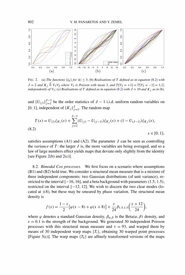
802 V. M. PANARETOS AND Y. ZEMEL
FIG. 2. (a) The functions {ζk} for |k| ≤ 3; (b) Realisations of T defined as in equation (8.2) with
J = 2 and Kjd= V1V2 where V1 is Poisson with mean 3, and P[V2 = +1] = P[V2 = −1] = 1/2,
independently of V1; (c) Realisations of T defined as in equation (8.2) with J = 10 and Kj as in (b).
and {U(j)}J−1j=1 be the order statistics of J − 1 i.i.d. uniform random variables on
[0,1], independent of {Kj }Jj=1. The random map
T (x) = U(1)ζK1(x) +J−1∑j=2
(U(j) − U(j−1))ζKj(x) + (1 − U(J−1))ζKJ
(x),
(8.2)x ∈ [0,1],
satisfies assumptions (A1) and (A2). The parameter J can be seen as controllingthe variance of T : the larger J is, the more variables are being averaged, and so alaw of large numbers effect yields maps that deviate only slightly from the identity[see Figure 2(b) and 2(c)].
8.2. Bimodal Cox processes. We first focus on a scenario where assumptions(B1) and (B2) hold true. We consider a structural mean measure that is a mixture ofthree independent components: two Gaussian distributions (of unit variance), re-stricted to the interval [−16,16], and a beta background with parameters (1.5,1.5),restricted on the interval [−12,12]. We wish to discern the two clear modes (lo-cated at ±8), but these may be smeared by phase variation. The structural meandensity is
f (x) = 1 − ε
2
[ϕ(x − 8) + ϕ(x + 8)
] + ε
24β1.5,1.5
(x + 12
24
),
where ϕ denotes a standard Gaussian density, βα,β is the Beta(α,β) density, andε = 0.1 is the strength of the background. We generated 30 independent Poissonprocesses with this structural mean measure and τ = 93, and warped them bymeans of 30 independent warp maps {Ti}, obtaining 30 warped point processes[Figure 3(c)]. The warp maps {Tk} are affinely transformed versions of the maps

AMPLITUDE AND PHASE VARIATION 803
FIG. 3. (a) Thirty warped bimodal densities, with the structural mean bimodal density 93 × f
in solid black; (b) Their corresponding distribution functions, with the structural mean distributionfunction in solid black; (c) Thirty Cox processes, constructed as follows: first we generate �i as i.i.d.Poisson processes with mean density f , then we warp them by forming T#�i , where T are the mapsappearing in Figure 2(b).
shown in Figure 2(b) according to the mapping
g(x) → 32g
(x + 16
32
)− 16
in order to re-scale their support to [−16,16]. Recall that the warp maps inFigure 2(b) were generated using the definition in equation (8.2), taking J = 2and Kj are i.i.d., distributed as V1V2, where V1 is Poisson with mean 3, andP[V2 = +1] = P[V2 = −1] = 1/2, independently of V1. These correspond torather violent phase variation, as can be seen by the plots of the conditional den-sity/distribution of the warped processes given the corresponding Ti in Figure 3(a)and 3(b).
Using the 30 warped spike trains depicted in Figure 3(c), we construct the “reg-ularised Fréchet–Wasserstein” estimator as described in Section 4. A slight devia-tion is that we use a Gaussian kernel with bandwidth chosen by unbiased cross val-idation, rather than the special kernels developed for the asymptotic theory (withno essential effect on finite sample performance). We thus obtain estimates of thewarp maps {Ti}30
i=1 (using the definitions in Section 4.4), depicted in Figure 4(b),which can be used to register the point processes (Figure 5). The final estimateof the structural mean distribution function (the regularised Fréchet–Wassersteinestimator) is depicted in Figure 4(a), and contrasted with the true structural CDF,as well as with the naive estimate produced by ignoring warping and averagingthe empirical distributions across trains. We notice that the regularised Fréchet–Wasserstein estimator performs quite well at discerning the two modes of the struc-tural mean measure, in contrast with the naive estimator which seems to fail to re-solve them. This effect is more clearly portrayed in Figure 4(c), which plots kernelestimators of structural mean density constructed using the original (warped) pointprocesses, and the registered point processes. It is important to remark that the mi-nor fluctuations in the density estimate observed are not related to our method
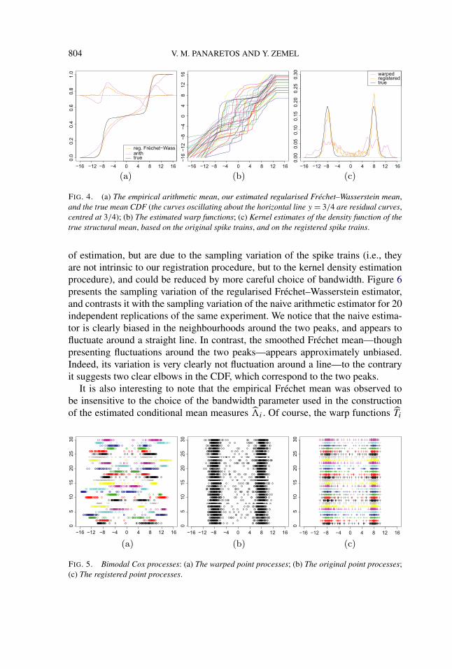
804 V. M. PANARETOS AND Y. ZEMEL
FIG. 4. (a) The empirical arithmetic mean, our estimated regularised Fréchet–Wasserstein mean,and the true mean CDF (the curves oscillating about the horizontal line y = 3/4 are residual curves,centred at 3/4); (b) The estimated warp functions; (c) Kernel estimates of the density function of thetrue structural mean, based on the original spike trains, and on the registered spike trains.
of estimation, but are due to the sampling variation of the spike trains (i.e., theyare not intrinsic to our registration procedure, but to the kernel density estimationprocedure), and could be reduced by more careful choice of bandwidth. Figure 6presents the sampling variation of the regularised Fréchet–Wasserstein estimator,and contrasts it with the sampling variation of the naive arithmetic estimator for 20independent replications of the same experiment. We notice that the naive estima-tor is clearly biased in the neighbourhoods around the two peaks, and appears tofluctuate around a straight line. In contrast, the smoothed Fréchet mean—thoughpresenting fluctuations around the two peaks—appears approximately unbiased.Indeed, its variation is very clearly not fluctuation around a line—to the contraryit suggests two clear elbows in the CDF, which correspond to the two peaks.
It is also interesting to note that the empirical Fréchet mean was observed tobe insensitive to the choice of the bandwidth parameter used in the constructionof the estimated conditional mean measures i . Of course, the warp functions Ti
FIG. 5. Bimodal Cox processes: (a) The warped point processes; (b) The original point processes;(c) The registered point processes.

AMPLITUDE AND PHASE VARIATION 805
FIG. 6. (a) Comparison of our estimated regularised Fréchet–Wasserstein mean, and the true meanCDF, for 20 independent replications of the experiment; (b) Comparison of the arithmetic mean, andthe true mean CDF, for the same 20 replications; (c) Superposition of (a) and (b). In all three cases,the curves oscillating about the horizontal line y = 3/4 are residual curves, centred at 3/4.
themselves (and hence the registered processes) would depend on this parameter,since these couple i and λ—and while the latter is insensitive to the choice ofbandwidth parameter, the former is clearly not.
Further simulations carried out in the supplementary material [27] reaffirm thesefindings for different “sample sizes” τ and choices of smoothing parameter. Fur-thermore, numerical comparisons also carried out in the supplement suggest thatFréchet–Wasserstein registration outperforms Fisher–Rao registration (carried outas in [36] at the level of CDFs), in terms of how close the registered processes areto the original point processes (prior to warping), where “closeness” is measuredby means of the �2 distance of the ordered points. This is not surprising givenour unbiasedness considerations (Proposition 3), since the Fisher–Rao estimator isgenerally not d-unbiased.
8.3. Triangular Cox processes. We now treat a second scenario that some-what deviates from our model assumptions, because it involves linear warp func-tions. Consequently, phase variation can also be seen at the level of densities (seeSection 3.4). Consider the family of triangular densities of support length 2h andheight 1/h, and their corresponding distribution functions (see Figure 7)
fh(t) = 1
h
(1 − 1
h|t |
), |t | ≤ h,h > 0,
Fh(t) =
⎧⎪⎪⎨⎪⎪⎩1
2h2 (t + h)2, −h ≤ t ≤ 0,
1 − 1
2h2 (h − t)2, 0 ≤ t ≤ h.
Our example will consist in phase varying Poisson processes, with structuralmean distribution equal to F1 (i.e., the triangular distribution function with h = 1).
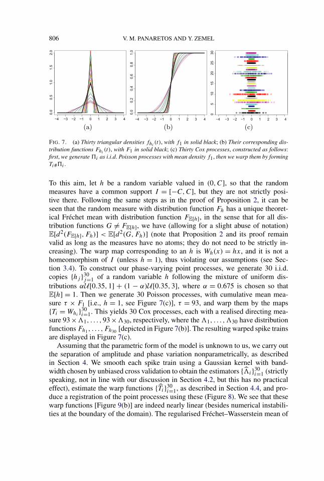
806 V. M. PANARETOS AND Y. ZEMEL
FIG. 7. (a) Thirty triangular densities fhi(t), with f1 in solid black; (b) Their corresponding dis-
tribution functions Fhi(t), with F1 in solid black; (c) Thirty Cox processes, constructed as follows:
first, we generate �i as i.i.d. Poisson processes with mean density f1, then we warp them by formingTi#�i .
To this aim, let h be a random variable valued in (0,C], so that the randommeasures have a common support I = [−C,C], but they are not strictly posi-tive there. Following the same steps as in the proof of Proposition 2, it can beseen that the random measure with distribution function Fh has a unique theoret-ical Fréchet mean with distribution function FE[h], in the sense that for all dis-tribution functions G �= FE[h], we have (allowing for a slight abuse of notation)E[d2(FE[h],Fh)] < E[d2(G,Fh)] (note that Proposition 2 and its proof remainvalid as long as the measures have no atoms; they do not need to be strictly in-creasing). The warp map corresponding to an h is Wh(x) = hx, and it is not ahomeomorphism of I (unless h = 1), thus violating our assumptions (see Sec-tion 3.4). To construct our phase-varying point processes, we generate 30 i.i.d.copies {hj }30
j=1 of a random variable h following the mixture of uniform dis-tributions αU[0.35,1] + (1 − α)U[0.35,3], where α = 0.675 is chosen so thatE[h] = 1. Then we generate 30 Poisson processes, with cumulative mean mea-sure τ × F1 [i.e., h = 1, see Figure 7(c)], τ = 93, and warp them by the maps{Ti = Whi
}30i=1. This yields 30 Cox processes, each with a realised directing mea-
sure 93×1, . . . ,93×30, respectively, where the 1, . . . ,30 have distributionfunctions Fh1, . . . ,Fh30 [depicted in Figure 7(b)]. The resulting warped spike trainsare displayed in Figure 7(c).
Assuming that the parametric form of the model is unknown to us, we carry outthe separation of amplitude and phase variation nonparametrically, as describedin Section 4. We smooth each spike train using a Gaussian kernel with band-width chosen by unbiased cross validation to obtain the estimators {i}30
i=1 (strictlyspeaking, not in line with our discussion in Section 4.2, but this has no practicaleffect), estimate the warp functions {Ti}30
i=1, as described in Section 4.4, and pro-duce a registration of the point processes using these (Figure 8). We see that thesewarp functions [Figure 9(b)] are indeed nearly linear (besides numerical instabili-ties at the boundary of the domain). The regularised Fréchet–Wasserstein mean of
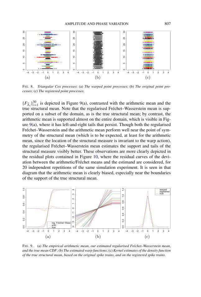
AMPLITUDE AND PHASE VARIATION 807
FIG. 8. Triangular Cox processes: (a) The warped point processes; (b) The original point pro-cesses; (c) The registered point processes.
{Fi}30i=1 is depicted in Figure 9(a), contrasted with the arithmetic mean and the
true structural mean. Note that the regularised Fréchet–Wasserstein mean is sup-ported on a subset of the domain, as is the true structural mean; by contrast, thearithmetic mean is supported almost on the entire domain, which is visible in Fig-ure 9(a), where it has left-and-right tails that persist. Though both the regularisedFréchet–Wasserstein and the arithmetic mean perform well near the point of sym-metry of the structural mean (which is to be expected, at least for the arithmeticmean, since the location of the structural measure is invariant to the warp action),the regularised Fréchet–Wasserstein mean estimates the support and tails of thestructural measure visibly better. These observations are more clearly depicted inthe residual plots contained in Figure 10, where the residual curves of the devi-ation between the arithmetic/Fréchet means and the estimand are considered, for20 independent repetitions of the same simulation experiment. It is seen in thatdiagram that the arithmetic mean is clearly biased, especially near the boundariesof the support of the true structural mean.
FIG. 9. (a) The empirical arithmetic mean, our estimated regularised Fréchet–Wasserstein mean,and the true mean CDF; (b) The estimated warp functions; (c) Kernel estimates of the density functionof the true structural mean, based on the original spike trains, and on the registered spike trains.

808 V. M. PANARETOS AND Y. ZEMEL
FIG. 10. (a) Comparison of our estimated regularised Fréchet–Wasserstein mean, and the truemean CDF, for 20 independent replications of the experiment; (b) Comparison of the arithmeticmean, and the true mean CDF, for the same 20 replications; (c) Superposition of (a) and (b). In allthree cases, the curves oscillating about the horizontal line y = 1/2 are residual curves, centred at1/2.
To gauge the effectiveness of the registration carried out, we also constructedkernel estimators of the density of the structural mean, based on the original(warped) point processes, and on the registered (aligned) point processes. Theseare shown in Figure 9(c). They illustrate that the density estimate based on theraw data overestimates the mode as well as the tails of the true density, whereasthe density estimate based on the registered data fits both the bulk and the tailsof the density quite nicely. As in the previous example, the minor fluctuations ofthese density estimates are not intrinsic to our registration procedure, but to thekernel density estimation procedure.
Stability of the estimated structural mean CDF with respect to the smoothingparameter was also observed in this example, and persisted in additional simula-tions (presented in the supplementary material [27]), where different sample sizeswere also considered. Simulation comparisons showed that also in this scenarioour approach performs at least as well as the Fisher–Rao approach in terms ofregistration of the point processes.
9. Discussion. We have introduced a framework formalising the confoundingof amplitude and phase variation in point process data, and demonstrated how thiscan be used for their consistent nonparametric separation on the basis of indepen-dent realisations thereof. The key ingredient of our approach was the observationthat for the point process warping problem, the classical functional data assump-tions on warp functions are equivalent to the geometry of the Monge problem ofoptimal transportation.
A particularly attractive aspect of the present framework is that it yields an iden-tifiable setup, with a clear notion of over/under registration through the concept ofbias. Indeed, we prove that consistent estimation of the warp functions is possible
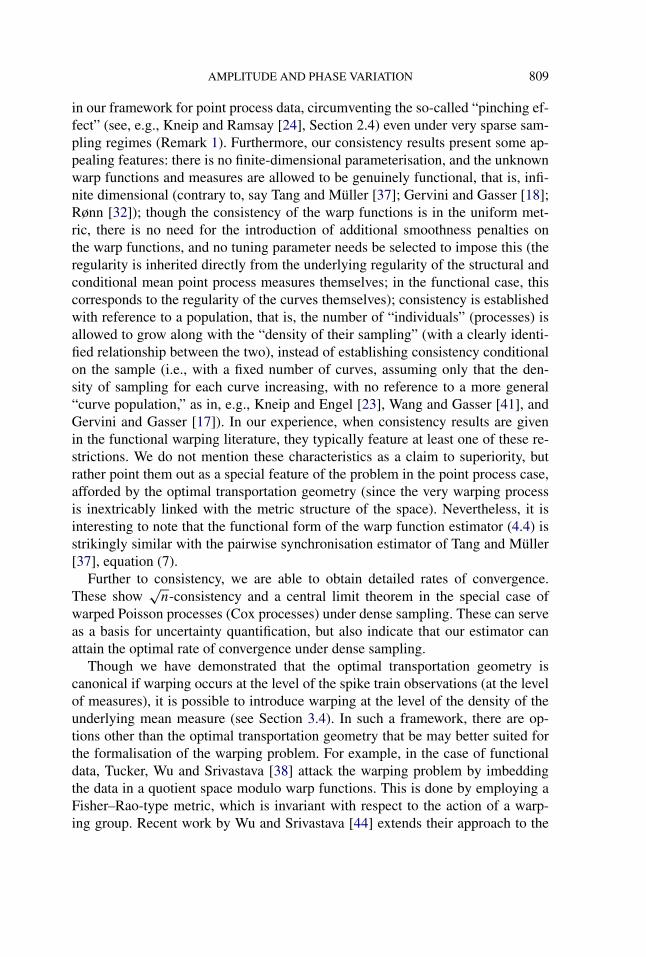
AMPLITUDE AND PHASE VARIATION 809
in our framework for point process data, circumventing the so-called “pinching ef-fect” (see, e.g., Kneip and Ramsay [24], Section 2.4) even under very sparse sam-pling regimes (Remark 1). Furthermore, our consistency results present some ap-pealing features: there is no finite-dimensional parameterisation, and the unknownwarp functions and measures are allowed to be genuinely functional, that is, infi-nite dimensional (contrary to, say Tang and Müller [37]; Gervini and Gasser [18];Rønn [32]); though the consistency of the warp functions is in the uniform met-ric, there is no need for the introduction of additional smoothness penalties onthe warp functions, and no tuning parameter needs be selected to impose this (theregularity is inherited directly from the underlying regularity of the structural andconditional mean point process measures themselves; in the functional case, thiscorresponds to the regularity of the curves themselves); consistency is establishedwith reference to a population, that is, the number of “individuals” (processes) isallowed to grow along with the “density of their sampling” (with a clearly identi-fied relationship between the two), instead of establishing consistency conditionalon the sample (i.e., with a fixed number of curves, assuming only that the den-sity of sampling for each curve increasing, with no reference to a more general“curve population,” as in, e.g., Kneip and Engel [23], Wang and Gasser [41], andGervini and Gasser [17]). In our experience, when consistency results are givenin the functional warping literature, they typically feature at least one of these re-strictions. We do not mention these characteristics as a claim to superiority, butrather point them out as a special feature of the problem in the point process case,afforded by the optimal transportation geometry (since the very warping processis inextricably linked with the metric structure of the space). Nevertheless, it isinteresting to note that the functional form of the warp function estimator (4.4) isstrikingly similar with the pairwise synchronisation estimator of Tang and Müller[37], equation (7).
Further to consistency, we are able to obtain detailed rates of convergence.These show
√n-consistency and a central limit theorem in the special case of
warped Poisson processes (Cox processes) under dense sampling. These can serveas a basis for uncertainty quantification, but also indicate that our estimator canattain the optimal rate of convergence under dense sampling.
Though we have demonstrated that the optimal transportation geometry iscanonical if warping occurs at the level of the spike train observations (at the levelof measures), it is possible to introduce warping at the level of the density of theunderlying mean measure (see Section 3.4). In such a framework, there are op-tions other than the optimal transportation geometry that be may better suited forthe formalisation of the warping problem. For example, in the case of functionaldata, Tucker, Wu and Srivastava [38] attack the warping problem by imbeddingthe data in a quotient space modulo warp functions. This is done by employing aFisher–Rao-type metric, which is invariant with respect to the action of a warp-ing group. Recent work by Wu and Srivastava [44] extends their approach to the

810 V. M. PANARETOS AND Y. ZEMEL
case of spike trains, by smoothing the spike trains and considering them as densi-ties in the Fisher–Rao space. This geometry may be more natural than the optimaltransportation one to model phase variation at the level of densities.
A natural question for further work is that of multivariate phase variation. Forexample, is the “canonicity” of the optimal transportation framework preserved,and can one fruitfully proceed in a similar manner? The key challenge in this caseis that, in the case of measures on subsets of Rd , d > 1, evaluation of the empiricalFréchet mean in closed form is impossible (see, e.g., Agueh and Carlier [1]). Ap-proximations can be sought, for example, via Gaussian assumptions (Cuturi andDoucet [12]) or via reduction to several 1D problems (Bonneel et al. [8]). Indeed,during the final preparation of this manuscript, we became aware of interestingindependent work in parallel by Boissard, LeGuic and Loubes [7], who considerthe problem of estimating Wasserstein barycentres for measures on R
d , and de-fine “admissible” groups of deformations that mimic the 1D case, thus allowingfor consistent estimation and evaluation of the sample barycentre by calculatingsuccessive means between pairs (i.e., by an iterated barycentre).
Finally, it should be mentioned that once phase and amplitude variation havebeen separated, they could each be subjected to a further analysis of their own.The amplitude variation clearly would be analysed by means of linear PCA tools,along the lines described in Section 3.1. On the other hand, the phase variationcan be analysed by making further use of the geometrical properties described inSection 3.3: for instance, via tangent space PCA (see, e.g., Boissard, LeGuic andLoubes [7]) or via geodesic PCA (see, e.g., Bigot et al. [6]). Indeed, the form ofthe limiting covariance function in our central limit theorem (Theorem 3) suggeststhat strong connections can be established between Wasserstein PCA methodologyand the separation of amplitude and phase variation.
Acknowledgments. This paper grew out of work presented at the Mathemat-ical Biosciences Institute (Ohio State University), during the “Statistics of TimeWarping and Phase Variation” Workshop, November 2012. We wish to acknowl-edge the stimulating environment offered by the Institute. We are grateful to anAssociate Editor and three referees for their insightful and constructive comments.The paper has genuinely improved as a result of the review process.
SUPPLEMENTARY MATERIAL
“Amplitude and phase variation of point processes” (DOI: 10.1214/15-AOS1387SUPP; .pdf). The online supplement contains more detailed simulationexperiments.
REFERENCES
[1] AGUEH, M. and CARLIER, G. (2011). Barycenters in the Wasserstein space. SIAM J. Math.Anal. 43 904–924. MR2801182

AMPLITUDE AND PHASE VARIATION 811
[2] ANDERES, E. and CHATTERJEE, S. (2009). Consistent estimates of deformed isotropic Gaus-sian random fields on the plane. Ann. Statist. 37 2324–2350. MR2543694
[3] ANDERES, E. B. and STEIN, M. L. (2008). Estimating deformations of isotropic Gaussianrandom fields on the plane. Ann. Statist. 36 719–741. MR2396813
[4] ARRIBAS-GIL, A. and MÜLLER, H.-G. (2014). Pairwise dynamic time warping for event data.Comput. Statist. Data Anal. 69 255–268. MR3146893
[5] BICKEL, P. J. and FREEDMAN, D. A. (1981). Some asymptotic theory for the bootstrap. Ann.Statist. 9 1196–1217. MR0630103
[6] BIGOT, J., GOUET, R., KLEIN, T. and LOPEZ, A. (2013). Geodesic PCA in the Wassersteinspace. Available at arXiv:1307.7721.
[7] BOISSARD, E., LE GOUIC, T. and LOUBES, J.-M. (2015). Distribution’s template estimatewith Wasserstein metrics. Bernoulli 21 740–759. MR3338645
[8] BONNEEL, N., RABIN, J., PEYRÉ, G. and PFISTER, H. (2015). Sliced and Radon Wassersteinbarycenters of measures. J. Math. Imaging Vision 51 22–45. MR3300482
[9] CHIANG, C.-T., WANG, M.-C. and HUANG, C.-Y. (2005). Kernel estimation of rate functionfor recurrent event data. Scand. J. Stat. 32 77–91. MR2136803
[10] CHIOU, J.-M. and MÜLLER, H.-G. (2009). Modeling hazard rates as functional data for theanalysis of cohort lifetables and mortality forecasting. J. Amer. Statist. Assoc. 104 572–585. MR2751439
[11] CLAESKENS, G., SILVERMAN, B. W. and SLAETS, L. (2010). A multiresolution approach totime warping achieved by a Bayesian prior-posterior transfer fitting strategy. J. R. Stat.Soc. Ser. B. Stat. Methodol. 72 673–694. MR2758241
[12] CUTURI, M. and DOUCET, A. (2013). Fast computation of Wasserstein barycenters. Availableat arXiv:1310.4375.
[13] DALEY, D. J. and VERE-JONES, D. (2008). An Introduction to the Theory of Point Processes.Vol. II: General Theory and Structure, 2nd ed. Springer, New York. MR2371524
[14] DURRETT, R. (2010). Probability: Theory and Examples, 4th ed. Cambridge Univ. Press, Cam-bridge. MR2722836
[15] GANGBO, W. and SWIECH, A. (1998). Optimal maps for the multidimensional Monge–Kantorovich problem. Comm. Pure Appl. Math. 51 23–45. MR1486630
[16] GASSER, T. and KNEIP, A. (1995). Searching for structure in curve samples. J. Amer. Statist.Assoc. 90 1179–1188.
[17] GERVINI, D. and GASSER, T. (2004). Self-modelling warping functions. J. R. Stat. Soc. Ser.B. Stat. Methodol. 66 959–971. MR2102475
[18] GERVINI, D. and GASSER, T. (2005). Nonparametric maximum likelihood estimation of thestructural mean of a sample of curves. Biometrika 92 801–820. MR2234187
[19] HADJIPANTELIS, P. Z., ASTON, J. A. D. and EVANS, J. P. (2012). Characterizing fundamen-tal frequency in Mandarin: A functional principal component approach utilizing mixedeffect models. Journal of the Acoustical Society of America 131 4651–4664.
[20] JAMES, G. M. (2007). Curve alignment by moments. Ann. Appl. Stat. 1 480–501. MR2415744[21] KALLENBERG, O. (1986). Random Measures, 4th ed. Academic Press, London. MR0854102[22] KARR, A. F. (1991). Point Processes and Their Statistical Inference, 2nd ed. Probability: Pure
and Applied 7. Dekker, New York. MR1113698[23] KNEIP, A. and ENGEL, J. (1995). Model estimation in nonlinear regression under shape in-
variance. Ann. Statist. 23 551–570. MR1332581[24] KNEIP, A. and RAMSAY, J. O. (2008). Combining registration and fitting for functional mod-
els. J. Amer. Statist. Assoc. 103 1155–1165. MR2528838[25] LEHMANN, E. L. (1951). A general concept of unbiasedness. Ann. Math. Statistics 22 587–
592. MR0047296[26] MARRON, J. S., RAMSAY, J. O., SANGALLI, L. M. and SRIVASTAVA, A. (2014). Statistics
of time warpings and phase variations. Electron. J. Stat. 8 1697–1702. MR3273584

812 V. M. PANARETOS AND Y. ZEMEL
[27] PANARETOS, V. M. and ZEMEL, Y. (2015). Supplement to “Amplitude and phase variation ofpoint processes.” DOI:10.1214/15-AOS1387SUPP.
[28] RAMSAY, J. O. (2000). Functional components of variation in handwriting. J. Amer. Statist.Assoc. 95 9–15.
[29] RAMSAY, J. O. and LI, X. (1998). Curve registration. J. R. Stat. Soc. Ser. B. Stat. Methodol.60 351–363. MR1616045
[30] RAMSAY, J. O. and SILVERMAN, B. W. (2002). Applied Functional Data Analysis: Methodsand Case Studies. Springer, New York. MR1910407
[31] RAMSAY, J. O. and SILVERMAN, B. W. (2005). Functional Data Analysis, 2nd ed. Springer,New York. MR2168993
[32] RØNN, B. B. (2001). Nonparametric maximum likelihood estimation for shifted curves. J. R.Stat. Soc. Ser. B. Stat. Methodol. 63 243–259. MR1841413
[33] SAMPSON, P. D. and GUTTORP, P. (1992). Nonparametric estimation of non stationary spatialcovariance structure. J. Amer. Statist. Assoc. 87 108–119.
[34] SCHOENBERG, F. (1999). Transforming spatial point processes into Poisson processes.Stochastic Process. Appl. 81 155–164. MR1694573
[35] SENOUSSI, R., CHADŒUF, J. and ALLARD, D. (2000). Weak homogenization of point pro-cesses by space deformations. Adv. in Appl. Probab. 32 948–959. MR1808906
[36] SRIVASTAVA, A., WU, W., KURTEK, S., KLASSEN, R. and MARRON, J. S. (2011). Registra-tion of functional data using the Fisher–Rao metric. Available at arXiv:1103.3817v2.
[37] TANG, R. and MÜLLER, H.-G. (2008). Pairwise curve synchronization for functional data.Biometrika 95 875–889. MR2461217
[38] TUCKER, J. D., WU, W. and SRIVASTAVA, A. (2013). Generative models for functional datausing phase and amplitude separation. Comput. Statist. Data Anal. 61 50–66. MR3063000
[39] VILLANI, C. (2003). Topics in Optimal Transportation. Graduate Studies in Mathematics 58.Amer. Math. Soc., Providence, RI. MR1964483
[40] WANG, K. and GASSER, T. (1997). Alignment of curves by dynamic time warping. Ann.Statist. 25 1251–1276. MR1447750
[41] WANG, K. and GASSER, T. (1999). Synchronizing sample curves nonparametrically. Ann.Statist. 27 439–460. MR1714722
[42] WU, S., MÜLLER, H.-G. and ZHANG, Z. (2013). Functional data analysis for point processeswith rare events. Statist. Sinica 23 1–23. MR3076156
[43] WU, W. and SRIVASTAVA, A. (2013). Estimating summary statistics in the spike-train space.J. Comput. Neurosci. 34 391–410. MR3061973
[44] WU, W. and SRIVASTAVA, A. (2014). Analysis of spike train data: Alignment and comparisonsusing the extended Fisher–Rao metric. Electron. J. Stat. 8 1776–1785. MR3273594
SECTION DE MATHÉMATIQUES
ECOLE POLYTECHNIQUE FÉDÉRALE DE LAUSANNE
1015 LAUSANNE
SWITZERLAND
E-MAIL: [email protected]@epfl.ch