
American Education in the Age of Mass Migrations 1870-1930ftp.iza.org/dp3964.pdf · American...
47
IZA DP No. 3964 American Education in the Age of Mass Migrations 1870-1930 Fabrice Murtin Martina Viarengo DISCUSSION PAPER SERIES Forschungsinstitut zur Zukunft der Arbeit Institute for the Study of Labor January 2009
Transcript of American Education in the Age of Mass Migrations 1870-1930ftp.iza.org/dp3964.pdf · American...

IZA DP No. 3964
American Education in the Age of Mass Migrations1870-1930
Fabrice MurtinMartina Viarengo
DI
SC
US
SI
ON
PA
PE
R S
ER
IE
S
Forschungsinstitutzur Zukunft der ArbeitInstitute for the Studyof Labor
January 2009

American Education in the Age of
Mass Migrations 1870-1930
Fabrice Murtin Stanford University,
CEE, London School of Economics and CREST-INSEE
Martina Viarengo
Harvard University, London School of Economics
and IZA
Discussion Paper No. 3964 January 2009
IZA
P.O. Box 7240 53072 Bonn
Germany
Phone: +49-228-3894-0 Fax: +49-228-3894-180
E-mail: [email protected]
Any opinions expressed here are those of the author(s) and not those of IZA. Research published in this series may include views on policy, but the institute itself takes no institutional policy positions. The Institute for the Study of Labor (IZA) in Bonn is a local and virtual international research center and a place of communication between science, politics and business. IZA is an independent nonprofit organization supported by Deutsche Post Foundation. The center is associated with the University of Bonn and offers a stimulating research environment through its international network, workshops and conferences, data service, project support, research visits and doctoral program. IZA engages in (i) original and internationally competitive research in all fields of labor economics, (ii) development of policy concepts, and (iii) dissemination of research results and concepts to the interested public. IZA Discussion Papers often represent preliminary work and are circulated to encourage discussion. Citation of such a paper should account for its provisional character. A revised version may be available directly from the author.

IZA Discussion Paper No. 3964 January 2009
ABSTRACT
American Education in the Age of Mass Migrations 1870-1930*
This paper derives original series of average years of schooling in the United States 1870-1930, which take into account the impact of mass migrations on the US educational level. We reconstruct the foreign-born US population by age and by country of origin, while combining data on the flow of migrants by country and the age pyramids of migrants by country. Then we use original data on educational attainment in the nineteenth century presented in Morrisson and Murtin (2008) in order to estimate the educational level of US immigrants by age and by country. As a result, our series are consistent with the first national estimates of average schooling in 1940. We show that mass migrations have had a significant but modest impact on the US average educational attainment. However, the educational gap between US natives and immigrants was large and increased with the second immigration wave, a phenomenon that most likely fostered the implementation of restrictive immigration rules in the 1920s. JEL Classification: I2, J24, N70, O1 Keywords: education, migrations, economic history, economic development research Corresponding author: Martina Viarengo Program on Education Policy and Governance John F. Kennedy School of Government Harvard University 79 John F. Kennedy Street, Taubman 304 Cambridge, MA 02138 USA E-mail: [email protected]
* This paper has benefited from useful insights by Avner Greif, Claude Diebolt, Claudia Goldin, Pierre-Cyrille Hautcoeur, Christian Morrisson, Paul E. Peterson, Hugh Rockoff, Gianni Toniolo, Antonio Wendland, Jeffrey Williamson, Gavin Wright, as well as seminar participants at Rutgers University, Stanford University and Tor Vergata University. Murtin ackowledges financial support from the Mellon Foundation when he was hosted by Stanford Centre for the Study of Poverty and Inequality, as well as from the EU RTN Migration network when he was hosted by Tor Vergata University. Viarengo gratefully acknowledges the support of the Harvard’s Program on Education Policy and Governance.

1 Introduction
In the economic history literature most of the existing studies on the mass migra-
tions of the nineteenth century have focused on the evolution of migration flows,
their economic determinants and their consequences in both the country of origin
and the country of destination.
A more limited stream of the literature has looked at the characteristics of
migrants. In particular, an analysis of the composition of the stock of skills and
knowledge of the migrant population has never been achieved so far for that pe-
riod. In this paper, we aim to estimate the average educational level of US natives
as well as of immigrants over the period 1870-1930, hence obtaining the first con-
sistent series of average education among the whole US population.
This issue is of great importance in the context of developing an understanding
of the world economy in the first globalization era. As surveyed by Hatton and
Williamson (1998, 2005) and O’Rourke and Williamson (2000), mass migrations
have had many economic consequences on both the immigrant and the emigrant
countries, shifting an important part of the labor force from the labor-abundant
Old World to the labor-scarce New World. The United States have absorbed the
bulk of European emigration between 1820 and 1920, around 60%. The massive
flow of workers across the ocean had potentially some significant consequences on
the skill composition of the population. As the US were among the world leaders
in terms of literacy in 1870, it is true that migrants could have been viewed as
being unskilled by US standards.
2

In order to quantify the discrepancy in educational attainment between US
immigrants and native Americans, we use perpetual inventory methods to infer
average years of schooling among both populations, relying on Morrisson-Murtin
(2008) education database 1870-2000. As a result, we estimate the impact of
mass migrations on average years of schooling in the US population, and we find
that our 1870-1930 series are consistent with the first national estimate of average
years of schooling in 1940. In fact, this paper shows that the overall impact of
migrations has been at maximum a diminution of 0.8 average years of schooling
among the population aged 15-64, or 10 percentage points of enrolment rate in
8 years-long Primary. This gap is significant but still modest, because the 15-64
immigrants population never represented more than 25% of the US workforce.
However, it is true that the gap in average education was large between US na-
tives and immigrants. Among adults aged 15-39, In particular, it peaked with the
second wave of immigration at 4.27 average years of schooling in 1920, which
roughly represent a gap of more than 50 percentage points of Primary enrolment
rate. To draw a comparison, when native Americans had on average completed
Primary and a few years of high school, immigrants had completed slightly more
than half of Primary. With the start of the high school movement at the same
period, this gap had become unsustainable and was certainly an important mo-
tive behind the 1920s Immigration Quotas, which marked the start of selective
immigration to the US.
The paper proceeds as follows. Section two will describe briefly the literature
on the mass migrations of the nineteenth and early twentieth centuries. Then we
3

explain in section three how we have reconstructed the US population by age and
by country of origin using perpetual inventory methods. We present the data,
discuss the assumptions behind the construction of our series, and present the
results. Last section concludes.
2 Mass migrations to the United States 1820-1930
It is largely acknowledged in the existing literature that over the nineteenth and the
early twentieth century one of the fundamental factors leading Europeans to emi-
grate was land abundance in the New World. Certainly the pressure of a growing
population on a fixed amount of agricultural land play a key role in this decision as
emphasized by Livi Bacci (1991). Moreover, in the late nineteenth century many
holdings were subdivided in countries like Italy and this made it more difficult
for families to be self-sustained. This argument is supported by the empirical evi-
dence provided by Hatton and Williamson (1998, p.112) who find the share of the
labor force in agriculture to be a highly significant determinant of the decision to
migrate in Southern European countries, suggesting that the limited opportunities
in the lands of Southern Europe led to emigration.
Overall, immigration to the United States gradually shifted from Northern and
Western European countries to the Southern and Eastern ones in the late nine-
teenth century. The economic and political conditions in the countries of depar-
ture can provide an explanation for this timing. Also, the innovation of the steam
shipping on the North Atlantic and the reduction in the cost of the journey clearly
4

played a key role. It became easier over time for poorer people to make the move,
as well as to go back to their home country after some time. In this regard, im-
migration to the United States from the more peripherical regions of Europe often
became temporary in the late nineteenth century.
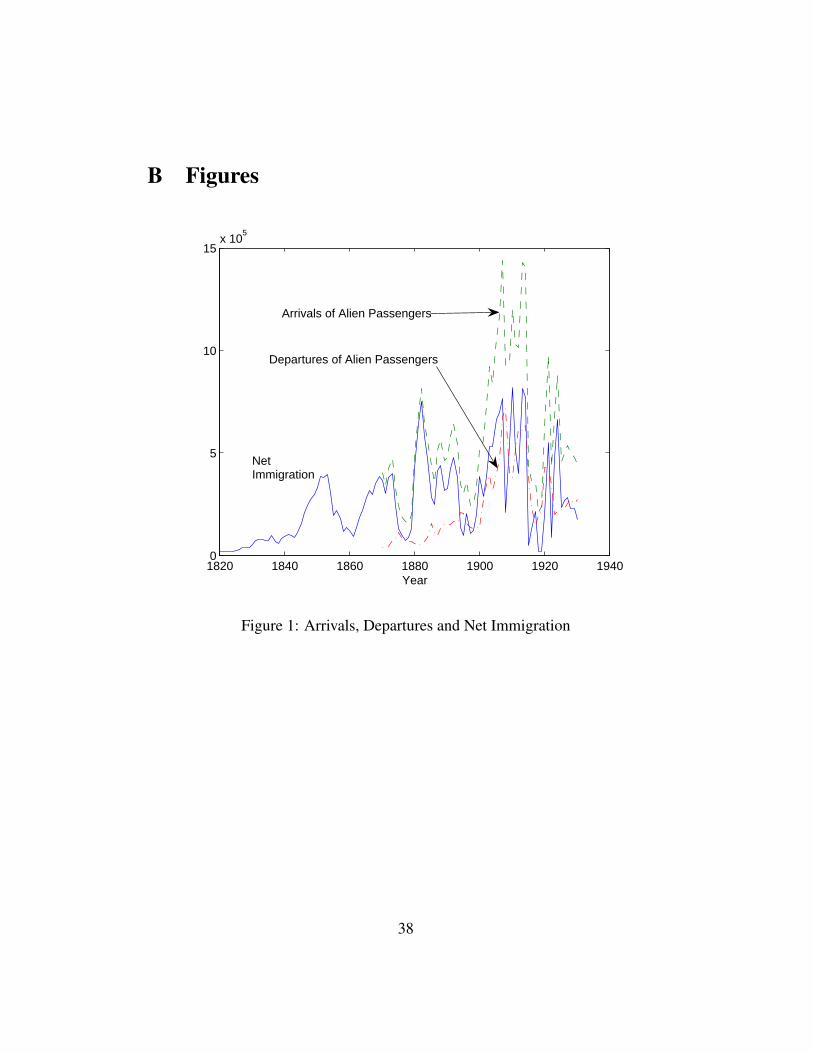
This is confirmed by Figure 1 that depicts the arrivals and the departures of
alien passengers as well as net immigration1. The height of the US net flow of
immigrants is reached before the beginning of the Great War and the recovery
from the war brings an increase in the flow of net immigration, which nevertheless
does not reach the pre-war levels.
Figures 2 and 3 depict the distribution by country of US immigrants in relative
terms, as described by HSUS. As previously described in other studies (Baines,
1991; Hatton and Williamson, 1998), two waves of mass immigration took place.
In the first one ranging roughly over the whole nineteenth century, immigration
from Ireland, Germany and the UK predominated, followed by Canada and Scan-
dinavia. After the Great Famine a substantial share of the Irish population mi-
grated to the United States. Average annual emigration increased dramatically
in Great Britain after 1880 but the greatest share of emigrants was directed to
Canada in this period. Emigration from Nordic countries like Norway, Sweden
and Denmark can be considered to be largely due to the poor economic condi-
tions of these countries in the second half of the nineteenth century. Then, at the
eve of the twentieth century, US immigration has been dominated by Eastern and
1Data are taken fron the Historical Statistics of the United States (2006), quoted hereafter asHSUS. Until 1930, a large majority of the arrivals of alien passengers corresponds to the arrivalsof US immigrants.
5

Southern Europe: Italy, Russia, Austria-Hungary, Poland. There were significant
differences in the Italian pattern of emigration: natives of Southern Italy mainly
migrated to the East Coast of North America whereas North-Eastern workers rep-
resented the bulk of the Latin American immigration, especially in Argentina.
What were the consequences of mass migrations on the composition of the US
population? Figure 4 shows the evolution of net immigration relative to the total
population increase as well as the evolution of the foreign born population with
respect to the total population. The first proportion has increased until the Civil
War, then decreased and increased again until the eve of the Great War. Then, a
dramatic drop occured. In this regard, immigration laws have been progressively
more restrictive in the United States and limited the foreign inflow. After the first
period of mass immigration, during which five million people left Europe to reach
the New World, between 1924 and 1965 the Origins Quota Act greatly reduced the
levels of immigration. This can be observed in the figure as starting shortly after
1920 when the legislation was implemented. The lowest level of net immigration
with respect to the population growth was reached during the Second World War
when strict immigration laws came into effect and also the volume of international
trade declined. After Second World War, the ratio of immigration to population
growth has gradually increased to reach the highest proportion ever observed in
2000.
The foreign born population relative to total population shows less important
fluctuations: it slightly increases until 1900, then declines until 1960 and increases
again. This will be an important point of the paper: as the latter proportion has
6

hardly exceeded 15%, one can conjecture a modest influence of mass migration on
the US average stock of education, unless the gap between migrants and natives
education has been very large. This will be investigated in next section.
3 Computing Average Years of Schooling in the United
States 1870-1930
In this section we present the framework that enables the reconstruction of the US
population by age and by country of origin between 1870 and 1930. It is based
on a perpetual inventory of the flow of migrants by age and by country. Then we
describe the data, and focus on underlying assumptions.
3.1 Statistical framework
We estimate average years of schooling among individuals aged 15-64 in the US
population and in the population of US natives only. They are respectively noted
ETott and EUS
t . We have
ETott =
∑n,k En,k,tPn,k,t∑
n,k Pn,k,t
(1)
where En,k,t is average years of schooling of US population of age n at time t
born in country k, and Pn,k,t the corresponding population. By convention k = 0
7

corresponds to the US natives, hence
EUSt =
∑n En,0,tPn,0,t∑
n Pn,0,t
(2)
Data on education by age and by country En,k,t are taken from from Morrisson-
Murtin (2008) as described below. Populations Pn,k,t are not observed and are re-
constructed via a perpetual inventory of net immigration. More precisely foreign-
born populations are constructed recursively in the following way
Pn,k,t = Pn−1,k,t−1Sn,k,t + FkAn,k,t for n, t ≥ 2, k > 0
P1,k,t = FkA1,k,t
where Sn,k,t stands for the conditional survival probability at age n and time t,
conditionally on having survived until age n − 1 (time t − 1), Fk the flow of net
immigration from country k, An,k,t the share of migrants of age n from country
k at time t. Initial conditions on the population in 1820 have little influence in
1870 and are set equal to zero2. We assume that once they have immigrated to the
United States, all populations from the various countries have the same survival
probability as US natives, namely that
∀k Sn,k,t = Sn,0,t (3)
2Only the 0-15 population resulting from pre-1820 migrations could have an influence in 1870.It will anyhow be very modest due to low life expectancy, the low share of children among immi-grants at that date, and small flows of migrants relatively to those of the future decades.
8

On the other hand, US native population, which includes children of immigrants,
is given by
Pn,0,t = Pn−1,0,t−1Sn,0,t for n, t ≥ 2
P1,0,t = BtS1,0,t (4)
where Bt is the number of births. In 1820 we make the simplifying assumption
that US citizens are all natives, hence we confound the US age pyramid with the
US natives age pyramid. In a further section we describe accurately the treatment
of missing data.
3.2 Data description
The data have been extracted from the Historical Statistics of the United States
(2006), Ferenczi and Willcox (1929 a,b) and Morrisson and Murtin (2008). The
record of immigration started in the United States in 1819 as a result of the Steer-
age Act, which required the master of each vessel reaching the United States to
declare name, age, sex and occupation of each passenger (HSUS, notes on table
Ad1-2). This record represents an invaluable source of information even though
the record of immigrants has changed over time3.
3For the flow of immigration we used the net flow of immigrants as calculated by the USCensus (HSUS Table Aa9-14), which is based on Kuznets-Rubin from 1870 (HSUS Table Ad21-24); for countries shares, we used data on immigrants by last country of residence (HSUS TableAd106-120) to proxy the origin country, as those series are the only one to go back in time asfar as 1820; foreign-born population by country of birth are taken from HSUS Table Ad354-443;US immigrants by age are taken from Table Ad226-230 (HSUS) where age groups have beenhomogeneized across time and statistics have been smoothed with a 10 years moving average; age
9

The major emigration countries were retained and some were aggregated. At
last we created eleven groups: Austria-Hungary, Canada, France, Germany, Ire-
land, Italy, Mexico, Poland, Russia-Finland, Sweden-Norway, the United King-
dom4. As a result, the total flow of immigrants from the retained countries rep-
resent 95.8% of total US immigration over the period 1820-1924 according to
Ferenczi-Willcox (1929, v.1 p.178). Migrations from Asia and some small Euro-
pean countries were neglected.
We present hereafter the data used in equations (1-4). In the first section Fig-
ures 2 and 3, we have already described the distribution of migrants by country of
origin Fk. Figure 5 shows how the US survival probabilities Sn,0,t have changed
over time. There are important differences between the survival probability at age
15 and the survival probability at age 40 conditional on survival at age 15 until
1880. This was mainly due to the very low life expectancy of the US population
and the very high infant mortality rates. Racial differential in mortality was also
important with the Afro-American population exhibiting shorter life expectancy
throughout all the period considered (for instance in 1910 the differential between
the number of infant deaths per 1,000 live births was 46).
Between 1850 and 1880, life expectancy fluctuated,5 mainly as a result of the
pyramids of immigrants from other countries are taken from Ferenczi and Willcox (1929a) whereage groups have been homogeneized.
4In flows of migrants and foreign-born populations, Austria-Hungary also included Czechoslo-vaquia, Albania and Yugoslavia; France included Belgium and Netherlands; Italy included Greece,Portugal and Spain; Mexico included Latin American countries and Caraibes; Russia-Finland in-cluded Bulgaria, Baltic countries, Romania and Turkey; Denmark was added to Sweden-Norway.Corresponding figures for education are population weighted averages. The names of the groupsderive from the major emigration countries among them.
5Fogel (1994) observed a decline in life expectancy between 1800 and 1860 and after a gradual
10

periodic epidemics and changes in the disease environment. The turning point
suggests that around 1880 the survival probability of the young population has
progressively improved, reaching 0.85 in 1920. It is not clear why 1880 happens
to be the turning point, but what is agreed upon by historians and demographers is
that “a new era in mortality history began around 1880”(Preston (1977, p. 165)6.
Data on average years of education En,k,t are depicted on Figure 6 for some
European countries and are issued from Morrisson and Murtin (2008). They use
Mitchell data (2003a,b,c) and estimate by perpetual inventory methods the average
years of Primary, Secondary and Tertiary schooling in 74 countries since 1870. As
many early enrolment figures were missing in the latter source, the authors used
Lindert (2004) as a secondary data source.
In Europe, Germany had an edge on the other countries in terms of average
years of schooling throughout the period. This is the outcome of early high enrol-
ment rates in Primary schooling, especially in Prussia. On Table 1 the diversity
of educational levels across emigration countries is striking. Four large emigra-
tion countries - Germany, Sweden, Norway and the United Kingdom - had high
levels of schooling in 1870, about 4.5 years on average. This roughly means that
75% of the population received 6 years of Primary schooling, or in other words
increase by considering the overall population.6Many factors seem to have played a role. First, the rapid mortality decline can be explained
by advances in living standards and better living conditions, improvements in the germ theoryof disease and certainly in the treatment of early-life disease. According to Nugent (1992, p.23)quoting a case study of Philadelphia over 1870-1930, epidemic diseases like smallpox, scarletfever and typhoid fever were no longer causes of death. Also, according to the latter author theUnited States by the 1880s had reached a modern demographic regime with lower birth and deathrates.
11

that the illiteracy rate was about 25%. On the other hand, Ireland, Central Europe
and Italy were lagging behind in 1870, with an educational level smaller than 3
average years of schooling.
It is also important to notice the change between 1870 and 1930. All countries
experienced a significant increase over these fifty years as a result of the imple-
mentation of gradual schooling reforms from the mid-nineteenth century such as
the introduction of compulsory schooling. Countries that started from lower lev-
els experienced the greatest increase: in Italy and Russia the estimated average
years of schooling increased by more than four times, in Ireland by more than
three. In Austria-Hungary and France the estimated stock of schooling doubled,
whereas in those countries which exhibited high levels in 1870 the increase was
more limited. In other words, convergence in years of schooling did occur during
that period, albeit not uniformly.
3.3 Assumptions
Some missing information in the data sources previously described led us to make
some assumptions. One of them is that immigrants were representative of their
home-country fellows in terms of average education. Second, missing data on
enrolment at school in emigration countries had to be supplemented by data inter-
polations in Morrisson and Murtin (2008). How influent are these interpolations
will be discussed below. Last, there are some missing data on age pyramids of
migrants and some unaccuracies in data of flows of migrants by country. Both
will be corrected using additional information taken from HSUS.
12

3.3.1 Education of migrants
A limited stream of the literature has looked at the characteristics of migrants.
Greenwood (2007) has looked at the age composition of US immigration and
found that the majority of migrants came from countries with a significant share
of the labor force in the primary sector and also with relatively low birth rates.
Baily (1983) and Erickson (1990) looked at the occupation of migrant workers.
They found some regularities in the ethnic group concentration across different
occupation. This is possibly one of the most revealing and valuable pieces of
socioeconomic information as occupation and wages provide information on both
the level of skills of the migrants and their market reward. Sandberg (1979, “the
impoverished sophisticated”) showed how people from the Nordic countries were
on average more educated than the other immigrants.
According to Williamson (2006), migrants were positively selected in two
ways. First, in terms of schooling: the evidence shows that immigrants from five
European countries to the United States between 1899 and 1909 exhibited higher
literacy rates than the average population that remained at home (Williamson,
2006, p.22). Moreover, immigrants were also positively selected in terms of in-
nate abilities. That is, there was a positive selection in terms of motivation, en-
trepreneurship, persistence and possibly with respect to other non-cognitive skills.
The over-representation of immigrants born between 1816 and 1850 among the
most successful businessmen supports this argument (Williamson, 2006, p.22).
As average years of schooling of migrants are obviously not available, we
will document this important question by focusing on occupations. For a handful
13

of countries, we have indeed some information on the share of migrants among
the emigrating population who work in the agriculture sector. For each coun-
try, we can compare this proportion to the national share of population working
in agriculture. It will tell us whether people from the primary sector are over
or under-represented in the emigrating population. As the bulk of illiteracy was
concentrated in rural areas, it will provide some suggestive evidences on how ed-
ucation of migrants compares with the national average7.
Table 2 reports the results. As visible, the evidence is scarce: 25 country-
period cells in total. It turns out that in Germany over the whole period, Italy in
1880, Finland in 1910 and Norway after 1910, both percentages are quite similar.
In all other countries excepted Austria, the percentage of workers in agriculture is
much lower in the emigrating population than in the country in general. Briefly,
farmers were less mobile. This is particularly marked in Norway, Sweden and the
British Isles.
To sum up, this suggests that farmers were under-represented in the migra-
tion population, and consequently that national average schooling constitutes most
likely a lower bound of migrants’ educational level. However, as this paper will
argue that mass migrations have entailed a modest impact on the US average
schooling level, we keep this assumption as a benchmark. It can be viewed as
7Unfortunately, it was not possible to compare the share of industry and services as classifi-cation turned out to be inconsistent between our two data sources: Ferenczi-Willcox (1929) formigrants, Mitchell (2003,a-b) for national figures. Mitchell acknowledges in preambule that thebuilding of such classification was difficult. He relies on the work of Bairoch et al. (1968), whowrote: “because of the frequent changes in criteria and methods used in census taking...it is prac-tically impossible to come up with statistics that are perfectly comparable in time and space”.
14

a conservative assumption in the sense that it probably slightly underestimates
immigrants educational level, hence overestimate their negative impact on US av-
erage schooling.
3.3.2 Education in emigration countries
Inferring average schooling of the population aged between 15 and 64 in 1870
requires the knowledge of past enrolment rates between 1810 and 1860 when a
perpetual inventory method is used. As shown by Table 3, countries differ in the
extent of available information on enrolment. For Austria-Hungary, France, Ger-
many, Italy, the United Kingdom and the United States enrolment figures were
available as soon as 1830 thanks to Lindert (2004). These are the countries for
which we have an accurate knowledge of average schooling in 1870. For other
countries, the first observation generally appeared in the course of the nineteenth
century, with Poland being an exception as enrolment is unknown until 1922. For
these countries, Morrisson-Murtin (2008) used ad-hoc assumptions on the enrol-
ment rates in 1820 and conducted a linear interpolation with the first observation.
If the first observed enrolment rate is low, as it is the case in Mexico and Finland,
then the measurement error will be of modest magnitude. Indeed, enrollment has
likely remained at very low levels between 1820 and the first observation8. If the
first observed enrolment rate is high, as it is the case in Canada and Scandinavia,
then the measurement error can be much higher.
8An examination of enrolment series for 74 countries demonstrate that growth in the enrolmentrate has been a common rule in any continent at any time, with a few exceptions occurring duringwars and the Great Depression.
15

The latter authors adopted the strategy of bounding this measurement error:
they calculated average schooling from 1870 in two extreme scenarios, one where
all past enrolment rates are equal to the first observed rate, another where enrol-
ment increases in the immediate past of the first observation at the highest speed
observed worldwide over the period 1820-1960 (+2% of enrolment rate in Primary
per year). The first scenario overestimates average schooling in the adult popula-
tion, and on the contrary the second scenario underestimates average schooling.
This therefore leaves us with a confidence interval for all countries, which is re-
ported on Table 1.
As expected, this confidence interval is very narrow in France, Germany, Italy
and the United Kingdom. It is much larger in Canada, Ireland, Mexico, Scandi-
navia, and above all Poland. However, Mexico and Poland excepted, the width of
the confidence interval has shrunk to 0 in 1930. This simply reflects that one has
information on any cohort of age.
In the following, we will use the upper and lower bounds of average schooling
of the various cohorts of age in order to gauge the measurement error that possi-
bly contaminates the US average schooling figure because of unknown European
enrolment rates.
3.3.3 Flows and Age Pyramids of Migrants
Some information on flows of migrants was corrected and some on age pyra-
mids of migrants was missing. As reported by the second column of Table 3, age
pyramids of immigrants start being available in 1850 in Austria-Hungary, 1860 in
16

France and Ireland, 1870 in Germany, Italy and Scandinavia, and 1900 in Finland.
Except for Italy, they are available on a decennial basis until the mentioned year.
So there is no data for the first half of the nineteenth century. However, we have
access to the age pyramids of migrants in the US regardless of their nationality.
We therefore make the simplifying assumption that immigrants from all countries
were distributed along the same age pyramid until 1840, the average age pyramid
of US immigrants. Then we interpolate with the first observed age pyramid. This
procedure is applied to Austria-Hungary, France, Germany, Ireland, Italy, Finland
and Scandinavia.
There are four countries for which no data, or very scarce data, are available.
These countries are Canada, Mexico, Poland and the United Kingdom. So we
have to form some ad-hoc assumptions on the age pyramids of their migrants. In
this regard, we have at our disposal two additional sources of information that
enable us to calibrate the assumptions adequately: the average age pyramid of US
migrants and total foreign-born population by country. In practice, we compare
these data with those stemming from our simulations and calibrate our assump-
tions in order to minimize the distance between predicted and observed variables9.
9More precisely, we interpolated the flow of migrants from Poland between 1894 and 1920as it was missing in the data. Foreign-born population from Austria-Hungary turned out to belargely overestimated with very high flows of migrants between 1874 and 1894; we applied an ad-hoc statistical correction, lessening those flows by 30%, which fit the corresponding foreign-bornpopulation; Mexican immigration is known to be under-reported (see notes of HSUS Table Ad1-2)with a share of US immigration smaller than 0.5% between 1835 and 1910; we interpolated thisshare over the latter period, augmenting it at about 2%. The UK had only sparse data (the shareof children 0-14); so we assumed that its age pyramid was intermediary between that of Germany,where the share of children is high, and Ireland, where the latter share is low, reflecting a blendof familial and economic migrations. Canada was inputed the average US age pyramid. Data onItaly were sparse between 1870 and 1920 and were unable to account for the prewar peak in adult
17

4 Results
4.1 The US population by age and country of origin
Let us present first the results of the latter calibration exercise. Averaging over
the country dimension k, one obtains An,.,t the simulated age pyramid of migrants
regardless of the country of origin. It is compared with the observed one on Fig-
ures 7 and 8, and the fit turns out to be almost perfect. This supports the view
that the procedure has successfully captured the age dimension of migration flows
by country. The graph depicts the high level and slow decline of the proportion
of children aged 0-15 among US immigrants over the period 1840-1880, then its
massive drop until First World War, and its afterwar recovery. Similarly, we cap-
ture the rise in the proportion of young adults among US immigrants in the late
1890s, and its decrease after the war.
Second, by summing over age dimension n one gets∑
n Pn,k,t the population
born in country k living in the US at time t, regardless of its age. All data are
summarized into 5 years averages. Figure 9 reflects the very good performance
of the procedure overall as well as in individual cases; indeed, the correlation be-
tween predicted and observed foreign-born populations appears to be very high:
so in addition to the age dimension, our procedure captures the origin country
dimension of migration flows. Only the Polish population, and the Mexican one
in a lesser extent, seem to have been underestimated; not surprisingly the United
migration; consequently it was inputed the Finish age pyramid that was roughly compatible duringthis period, as witnessed by the share of 0-14 children in 1900 and 1910.
18

Kingdom is somewhat problematic for several quinquennial periods. But over-
all, the correlation between predicted and observed populations is very high. As
shown by Table 3, eight countries over eleven have a level of correlation higher
than 0.9. The average correlation is 0.94.
Besides, there seems to be no significant bias in the measurement errors of
total populations. Figure 10 plots the empirical distribution of the relative mea-
surement error on total populations, estimated with a Gaussian kernel. Its mean is
0.16 and its standard error 0.70. Its positive mean can be explained by the exis-
tence of some outliers on the right tail, corresponding to negligeable populations
that generate large relative errors.
As expected, the foreign-born population is well captured as proved by Fig-
ure 11. This graph also shows that the total US population is well estimated,
albeit some slight overestimation in the afterwar. This indicates that the US na-
tive population is well reproduced by the a simple dynamical system based on the
knowledge of births and quinquenial survival probabilities. The outflow of US
emigrants to Canada seems to be therefore negligeable.
Table 4 addresses the age structure and relative importance of the various
groups. The share of the country-born population in US population in 1870 (first
column) is a good indicator of the timing of migration. As expected, Germany,
Ireland and the UK constitute the bulk of foreign-born population at that date.
Sixty years later, the foreign-born population is much more diverse as the largest
group of immigrants, Italians, represent only 2.1% of the US population. How-
ever, this imperfectly reflects the relative shares of “communities” as children of
19

migrants born in the US are classified as Americans. The share of young adults
is very high in most countries, but it varies across countries. This is related to
the type of migration. In 1870, countries like Austria-Hungary, Germany, Italy
and Sweden had a high proportion of children and this is explained by the “fa-
milial” type of immigration whereas Ireland represents the “economic” type of
immigration, which prevailed at the end of the period.
4.2 Education in the United States 1870-1930
Let us now turn to our final result, presented in the last Table and graph. The
confidence interval of US average years of schooling deriving from uncertain en-
rolment rates in Europe is reported on Figure 12 and is very narrow. This figure
also reports the average years of schooling as inferred from the first national sur-
vey by the US Census from 1940. Census estimates are fully in line with our serie
and extrapolate it naturally in 1940, 1950 and 1960. It is a strong confirmation
that our procedure has derived some credible series of average schooling among
the US population.
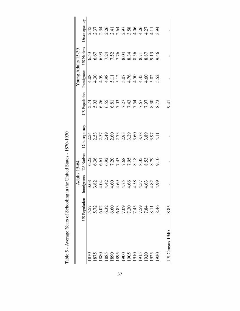
Table 5 shows for the first time the average education of US natives, of US
immigrants and of US population for both the 15-64 and the 15-39 age groups over
the period 1870-1930. It also reports the discrepancy between immigrants and
natives average education. It is no mystery that US natives were more educated:
the gap is equal to 2.54 average years of schooling in 1870, equivalent to a 30%
enrolment rate gap in an 8-years long Primary. This discrepancy is important,
but the composition effect is limited because the foreign-born population aged
20

between 15 and 64 years weighted 25.6% of the 15-64 US population, a share that
continuously decreased to reach 15.6% in 1930. As a result, average schooling
in the US is diminished from 6.22 years to 5.57 years in 1870, or a 0.65 years
gap - approximatively 8% of Primary enrolment rate in the population. This gap
is significant, but somewhat modest. We find the same result in the young adults
population: immigrants had on average 4.08 years of schooling versus 6.53 for
the natives of the same age group, a 2.45 years gap. The compositional impact
was a reduction of 0.79 average years of schooling on the 15-39 US population.
Interestingly, the discrepancy between 15-64 US natives and immigrants has
continuously increased from 1885. Similarly, a look at the 15-39 population re-
veals that the educational gap among young adults has decreased in the 1870s,
then rised again and peaked at a very large 4.27 value in 1920. This represents
more than a 50 percentage points discrepancy in enrolment rates in a 8-years long
Primary between natives and immigrants.
How do the latter figures compare with early evidence on educational attain-
ment in the US? Although many sources do exist (e.g., state level administrative
records, US census, state censuses and Current Population Survey) they are not
available for each geographical area the level of accuracy10 varies across states
(Goldin, 1999). The 1915 Iowa State Census represents an exception to the
paucity of data available11 The state of Iowa started twenty-five years earlier than10In this regard, statistics are not consistently recorded across states (e.g., in some states en-
rollment rates have been recorded only for some age-groups, some education data series folowthe school rather than the calendar year) and more in general these education data do not showthe ”years of schooling” of the population and appear inflated when comparing these to the actualoccupations.
11Also, the state of South Dakota adopted the same model to record the educational level of the
21

the other states to introduce questions on educational attainment in the census.
Moreover, the 1915 Iowa State Census sample is large and derived from a true
population census12. According to Goldin and Katz (2000) the Iowa State is rep-
resentative for the United States as educational wage differentials follow a similar
trend between 1940 and 1960. As a matter of facts, Iowa estimates are roughly
consistent with our figures. That is, average years of schooling for men, 25-49
years-old, were equal to 8.61 and to 8.98 for women in Iowa in 1915 (Goldin and
Katz, 2000, Table 1). At the same date, we calculate average years of schooling
for the 15-39 age band to be equal to 8.71 for US natives and 7.67 when migrants
are taken into account. As the latter authors acknowledge that the occupations in
Iowa were not representative of occupations at national levels, these figures appear
to be consistent with each other.
5 Immigration Laws, Education and the
Americanization Process of Immigrants
Immigration was nearly unrestricted in the nineteenth century13. Things came
to an end at the turn of the century when a series of laws were implemented to
limit the number of immigrants. The new legislation aimed at increasing the num-
population.12For an extensive review of the data sources over the nineteenth century, please refer to the
Historical Statistics of the United States and Goldin (1999).13With the exception of the 1882 Chinese Exclusion Act which imposed restrictions on im-
migration from Asia. According to Foreman-Peck (1992), this restriction was motivated by thefact that workers from Asia were mainly unskilled and would have substituted the American laborforce rather than complementing domestic labor.
22
ber of excludable categories by banning Asians, imposing passport requirement,
and introducing a sort of selection on the quality of immigrants. In an insightful
analysis Goldin (1994) examines the driving forces leading to the restriction of
immigration and shows how both labor and capital turned against immigration as
a result of the depression of the 1890s. O’Rourke and Williamson (2000) com-
plement this analysis by separating the short and long-run fundamentals that led
to the restriction of immigration. The passage of the legislation anti-immigration
was concentrated in less than ten years and three Acts represent the core of the
change in policy.
First, with the introduction of the Literacy Test in 1917, immigrants were re-
quired to read and write a language which did not have to be English. This piece
of legislation was the result of the report of the Immigration Commission headed
by Senator William Dillingham which concluded that the new immigrants, who
came from Italy, Poland, Hungary, Russia and Eastern Europe, did not assimilate
as easily as the ones who were coming from Northern and Western Europe during
the previous wave of immigration. Goldin (1994) explains how calls for the liter-
acy test were given serious consideration much earlier than the text became law in
1917. In fact, as early as in 1897 the proposal passed the House and the Senate but
received a presidential veto. The same author explains how the literacy test was
implemented at a time when literacy was rising rapidly in Europe (Goldin, 1994,
p.226). Consequently, other active policy measures became necessary to impose
a restriction on the immigration flow.
Second, the Emergency Quota Act of 1921 by imposing restrictions based on
23

the nationality of immigrants marked a significant change in the U.S. immigration
policy. In this regard, the policy became much more restrictive, that is only a
number equal to three percent of the number of foreign-born residents of each
nationality who were living in the United States as recorded by the 1910 census
was allowed to enter the United States.
Third, the Immigration Act of 1924 was even more restrictive as it lowered the
quota to two percent and used the 1890 census. It aimed at keeping the current
ethnic distribution and was a response to the increased immigration from Southern
and Eastern Europe. The Act reduced the number of U.S. immigration visas and
allocated them on the basis of national origin. It introduced a distinction between
quota-nations and non-quota nations. As a result, only 4000 Italians per year were
allowed to enter, while annual flows were about 200 000 per year between 1900
and 1915. In contrast, 86% of the 165 000 permitted entries were from France,
Britain, Germany and other Northern European countries.
What were the economic motives behind the implementation of the latter re-
strictions? Timer and Williamson (1997) argue that the change in attitude towards
immigration has been a result of the change in quantity and quality of the for-
eign labor supply. That is, policy became more restrictive as a result of the in-
creased immigration rates and the increase in the proportion of workers coming
from lower-wage and lower human capital countries of Europe. Because it created
more inequality, especially at the bottom of the income distribution, immigration
was a source of social unrest. They find that the most important factor for the
United States was the ratio of the unskilled wage to per capita income. That is,
24

the main determinant of the switch in policy was the deterioration of the labor
market conditions. This reflected the interests of the low-skilled workers who
were against immigration as opposed to the interests of capital owners who sup-
ported immigration as this could have granted them access to cheaper labor force.
Therefore, as a result of the widening of the income gap between unskilled and
skilled workers, policy makers implemented a more restrictive immigration legis-
lation to protect the interests of the unskilled labor. The authors also find that the
quality of immigration has been more important than the quantity of immigration
in determining the policy change, that non-economic variables do not have much
explanatory power, and that policies were correlated across countries in the New
World.
Another argument supports the view that the low quality of immigration was
the key factor behind migration laws: continuous flows of young illiterate immi-
grants might have jeopardized the rising high school movement and the ongoing
Americanization process. As described extensively by Goldin (1999), enrolment
in high school accelerated in the 1920s, exactely at the same time immigration
laws were implemented. Policy makers emphasized the process of American-
ization at the time, a process that relied on investments into immigrants’ chil-
dren education. Before World War I, Americanization was part of the Progressive
movement’s broader efforts to construct a modern and cohesive social order, and
also part of a new national effort to cultivate patriotism among all Americans.
Therefore, one of the main objectives was to ensure the adherence to “American”
cultural norms. According to Claxton (1920, p.622) “Americanization [wa]s a
25

process of education, of winning the mind and heart through instruction and en-
lightenment” and according to Thompson (1920, p.582), “America [wa]s looking
forward with anxious hope to the school as the chief instrument for American-
ization”. These quotes are revealing of the great importance that was attached to
education in the process of americanization. In this regard, in the early 1900s pub-
lic schools began to adopt extra-curricular activities to introduce immigrants to the
American values, beliefs and overall culture. With the beginning of World War
I, the movement of Americanizing the immigrant became even more widespread
(Atzmon, 1958, p.76). From 1914 to 1920 the Bureau of Naturalization of the
Immigration and Naturalization Service set invitations to more than 200,000 nat-
uralization applicants and their wives for them to attend English classes and the
essentials of good citizenship (Atzmon, 1958, p.76). This “quest for conformity”
(Carlson, p.623) was central to the American society before 1930 as Americans
had great faith that education and other organized forms of social control could
transform other immigrants into productive citizens. In that respect, uneducated
immigrants were certainly a problem for lawmakers who expressed a desire for
a more homogeneous society. As the education of youth was significantly raised
at the time, ensuring a proper Americanization of immigrants’ children, flows of
unskilled migrants were certainly counter-productive from that perspective, and
one would conjecture that this political factor was partly responsible for the im-
plementation of immigration laws.
26

6 Conclusion
This paper assesses the impact of mass migrations on the average level of school-
ing in the United States over the period 1870-1930. We reconstruct the foreign-
born population by age and by country of origin using data on age pyramids of
migrants by country and flows of immigrants by country. Then we combine it to
original data on educational attainment taken from Morrisson and Murtin (2007).
As a result, we derive original series of average schooling over the period 1870-
1930, which take into account the compositional effect of mass migrations. Impor-
tantly, our series are consistent with the first national value of average schooling
obtained in 1940. Our results suggest that immigration is unlikely to have entailed
large variations in the educational level of the US labor force because immigrants
never represented more than 25% of the US workforce. However, the educational
gap between immigrants and natives increased with the second wave of immigra-
tion. According to O’Rourke and Williamson (2000) mass migration and trade
did play the critical role in contributing to convergence. Can these series help
in refining their analysis by addressing the skill content of the workforce more
accurately? We leave this question opened for future research.
27

References
[1] Atzmon E. (1958). The educational programs for immigrants in the United
States. History of Education Journal, vol. 9, no. 3, p.75-80.
[2] Baily S. (1983). The Adjustment of Italian Immigrants in Buenos Aires and
New York, 1870-1914. American Historical Review, Vol. 88, No. 2, pp. 1-
305.
[3] Baines D. (1991). Emigration from Europe 1815-1930, prepared for the Eco-
nomic History Society, London: Macmillan Press
[4] Bairoch, P. et al. (1968). La population active et sa structure, Bruxelles, Uni-
versite libre de Bruxelles.
[5] Cameron R. (1985). A New View of European Industrialization. Economic
History Review, Vol. 38, No. 1, pp. 1-23.
[6] Carlson R. A. (1984). The Americanization Syndrome: A Quest for Confor-
mity. New York: St. Martin’s Press.
[7] Claxton P.P. (1920). What is Americanization?. Washington DC: Commis-
sioner for Education’s Report, pp.2-3.
[8] Erickson C. J. (1990). Emigration from the British Isles to the U.S.A. in
1841: Part 11. Who were the English emigrants?. Population Studies, Vol.
44, pp. 21-40.
28
[9] Ferenczi I. and Willcox W. F. (1929a). International Migrations, vol. 1 Statis-
tics, New York: National Bureau of Economic Research
[10] Ferenczi I. and Willcox W. F. (1929b). International Migrations, vol. 2 Inter-
pretations, New York: National Bureau of Economic Research
[11] Fogel, R. W. (1994). Economic Growth, Population Theory, and Physiology:
The Bearing of Long-Term Processes on the Making of Economic Policy,
American Economic Review Vol. 84, No. 3, pp. 369-95.
[12] Foreman-Peck, J. (1992). A Political Economy of International Migration,
1815-1914. The Manchester School of Economic Social Studies, Blackwell
Publishing, vol. 60(4), pp. 359-76.
[13] Goldin, C. (1994). The Political Economy of Immigration Restriction: The
United States, 1890-1921. In C. Goldin and G. Libecap, eds., The Regu-
lated Economy: An Historical Analysis of Government and the Economy.
Chicago, IL: University of Chicago Press.
[14] Goldin, C. (1999). A Brief History of Education in the United States. NBER
Working Paper, Historical Series no. 119.
[15] Goldin, C. and L. Katz (2000). Education and Income in the Early Twentieth
Century: Evidence from the Prairies. Journal of Economic History (Septem-
ber 2000).
29
[16] Greenwood, M.J. (2007). Modeling the age and age composition of late 19th
century U.S. immigrants from Europe. Explorations in Economic History,
2007, vol. 44, issue 2, pp. 255-269.
[17] Hatton T.J and Williamson J.G. (1998). The Age of Mass Migration. Causes
and Economic Impact, Oxford: Oxford University Press.
[18] Hatton T.J and Williamson J.G. (2005). Global migration and the world
economy: two centuries of policy. MIT Press.
[19] Historical Statistics of the United-States (2006). Milennial Edition Online.
[20] Livi-Bacci M. (1991) Population and Nutrition. An Essay on European De-
mographic History, Cambridge: Cambridge University Press
[21] Lindert, P. (2004). Growing Public. Vol. 2. Cambridge U.P. Cambridge.
[22] Mitchell, B.R. (2003a). International Historical Statistics: the Americas
1750-1993. M.Stockton Press, New-York.
[23] Mitchell, B.R. (2003b). International Historical Statistics: Europe 1750-
1993. M.Stockton Press, New-York.
[24] Mitchell, B.R. (2003c). International Historical Statistics: Africa, Asia and
Oceania 1750-1993. M.Stockton Press, New-York.
[25] Morrison C. and F. Murtin (2008). The Century of Education. Paris School
of Economics Working Paper.
30

[26] Nugent W. (1992). Crossings, The Great Transatlantic Migrations, 1870-
1914. Bloomington Indianapolis: Indiana University Press.
[27] O’Rourke, K. H., A. M. Taylor, and J. G. Williamson (1996). Factor Price
Convergence in the Late Nineteenth Century. International Economic Re-
view, Vol. 37, No. 3, pp.499-530.
[28] O’Rourke, K. H. and J. G. Williamson (2000). Globalization and History:
the evolution of a 19th century atlantic economy. Cambridge, Mass.: MIT
Press.
[29] Preston S. H. (1977). Mortality Trends. Annual Review of Sociology, Vol. 3,
pp. 163-178.
[30] Ruggles S. and M. Sobek. (1998). User’s Guide: Integrated Public Use Mi-
crodata Series: Version 2.0. Minneapolis: Minnesota Population Center,
University of Minnesota.
[31] Sandberg, L. G. (1979). The case of the impoverished sophisticate: Human
capital and the Swedish economic growth before World War I, The Journal
of Economic History, Vol. 39, No.1, pp.225-241.
[32] Thompson F. V. (1920). The School as the instrument for nationalization,
here and elsewhere. In Immigration and Americanization, P. Davis (ed.),
Boston: Gynn and Company, pp.582-600.
31

[33] Timmer, A. and J. G. Williamson. Racism, Xenophobia or Markets? The Po-
litical Economy of Immigration Policy Prior to the Thirties. NBER Working
Paper No. 5867, January 1997.
[34] Williamson, J.G. (2006). Inequality and schooling responses. The Global-
ization forces: lessons from history. NBER WP 12553.
32

A TableTable 1 - Average Years of Schooling Among 15-64
1870 1930
Estimate Lower Bound Upper Bound Estimate Lower Bound Upper Bound
Austria-Hungary 2.4 1.8 2.7 4.9 4.9 4.9
Canada 4.5 4.2 7.0 8.6 8.6 8.6
France 4.0 4.0 4.2 8.0 8.0 8.0
Germany 5.4 5.3 5.4 7.9 7.9 7.9
Ireland 2.2 1.6 2.9 7.0 7.0 7.0
Italy 0.9 0.8 0.9 4.1 4.1 4.1
Mexico 0.6 0.0 1.5 1.6 1.4 1.6
Poland 1.7 0.1 4.4 4.5 2.8 5.2
Finland 0.5 0.1 0.7 2.0 2.0 2.0
Sweden-Norway 4.7 3.0 5.0 6.7 6.7 6.7
United Kingdom 3.8 3.8 4.1 6.8 6.8 6.8
33

Table 2 - Share of Agriculture in Migrants and National Population Occupations
1880 1890 1900 1910 1920
Austria Migrants - - 59.1 62.8 -
Natives 51.9 57.1 53.3 48.8 32.4
France Migrants 38.4 - - - -
Natives - - 43.4 40.3 38.6
Germany Migrants - - 36.4 28.1 21.9
Natives 42.6 - 35.7 28.4 23.6
Italy Migrants 44.3 52.1 41.7 32.0 41.9
Natives 54.0 - 58.2 54.2 54.8
Finland Migrants - 77.0 74.1 65.2 49.0
Natives 72.4 - - 69.0 67.8
Norway Migrants 8.2 16.1 23.9 42.1 35.8
Natives 38.6 56.0 48.0 48.6 43.5
Sweden Migrants - 19.1 28.7 31.8 29.5
Natives 58.9 65.8 53.1 47.8 44.2
British Isles Migrants 6.5 9.4 7.0 7.8 -
UK Natives 17.6 14.7 12 11.5 9.2
Ireland Natives 40.6 - - 42.9 -
34

Tabl
e3
-Ava
ilabl
eD
ata
and
Goo
dnes
sof
Fit
Firs
tObs
erva
tion
ofE
nrol
men
tO
bser
ved
Age
Pyra
mid
sof
Imm
igra
nts
Cor
rela
tion
Bet
wee
nPr
edic
ted
and
Obs
erve
dPo
pula
tions
Aus
tria
-Hun
gary
1830
1850→
1910
0.99
8C
anad
a18
68-
0.86
2Fr
ance
1830
1860→
1890
0.85
7G
erm
any
1830
1870→
1930
0.92
5Ir
elan
d18
5318
60→
1920
0.95
4It
aly
1830
1870
,192
00.
997
Mex
ico
1895
-0.
948
Pola
nd19
22-
0.97
9R
ussi
a-Fi
nlan
d18
8019
00→
1920
0.99
7Sw
eden
-Nor
way
1855
1870→
1920
0.98
8U
nite
dK
ingd
om18
30-
0.80
6U
nite
dSt
ates
1830
1820→
1930
-
All
--
0.94
3
35

Table 4 - Immigrants Population Characteristics - Country Shares in Percents
1870 1930
Population Share1 Children2 Young Adults3 Population Share1 Children2 Young Adults3
Austria-Hungary 0.0 21.8 55.3 1.3 1.0 31.6
Canada 0.7 12.9 61.5 1.2 8.5 60.4
France 0.8 5.4 48.0 0.3 5.5 37.2
Germany 5.2 12.3 56.1 1.1 4.9 26.9
Ireland 5.3 3.4 57.8 0.7 1.7 32.1
Italy 0.1 10.6 53.3 2.1 2.7 40.0
Mexico 0.4 8.0 53.4 0.6 8.9 58.5
Poland 0.0 3.9 19.0 0.7 3.2 50.5
Russia-Finland 0.0 3.5 14.8 1.5 0.6 37.9
Sweden-Norway 0.5 20.8 52.9 0.8 2.0 31.0
United Kingdom 3.3 10.1 59.6 1.0 2.9 38.3
All 16.4 8.8 56.8 11.1 3.4 39.91 Share of the country-born population in US population
2 Share of the country-born children population (0-14) in country-born US population (0-64)
3 Share of the country-born young adults population (15-39) in country-born US population (0-64)
36
Tabl
e5
-Ave
rage
Yea
rsof
Scho
olin
gin
the
Uni
ted
Stat
es-1
870-
1930
Adu
lts15
-64
You
ngA
dults
15-3
9U
SPo
pula
tion
Imm
igra
nts
US
Nat
ives
Dis
crep
ancy
US
Popu
latio
nIm
mig
rant
sU
SN
ativ
esD
iscr
epan
cy18
705.
573.
686.
222.
545.
744.
086.
532.
4518
755.
723.
826.
362.
535.
934.
306.
672.
3718
806.
024.
046.
612.
576.
264.
596.
932.
3418
856.
324.
426.
922.
496.
554.
987.
242.
2618
906.
604.
607.
202.
606.
815.
117.
522.
4118
956.
834.
697.
432.
737.
035.
127.
762.
6419
007.
094.
757.
682.
937.
275.
078.
042.
9719
057.
304.
667.
953.
297.
434.
768.
343.
5819
107.
454.
588.
183.
607.
544.
508.
564.
0619
157.
594.
578.
353.
787.
674.
458.
714.
2619
207.
844.
638.
533.
897.
974.
608.
874.
2719
258.
114.
828.
793.
978.
305.
029.
134.
1119
308.
464.
999.
104.
118.
735.
529.
463.
94
US
Cen
sus
1940
8.85
--
-9.
41-
--
37
B Figures
1820 1840 1860 1880 1900 1920 19400
5
10
15x 10
5
Year
Arrivals of Alien Passengers
Departures of Alien Passengers
NetImmigration
Figure 1: Arrivals, Departures and Net Immigration
38

1830 1840 1850 1860 1870 1880 1890 1900 1910 1920 19300
0.05
0.1
0.15
0.2
0.25
0.3
0.35
0.4
0.45
0.5
Year
Per
cent
age
of U
S Im
mig
ratio
n(1
0 ye
ars
mov
ing
aver
age)
France
UK
Ireland
Mexico
Canada
Germany
Figure 2: The First Wave of Immigration
1830 1840 1850 1860 1870 1880 1890 1900 1910 1920 19300
0.05
0.1
0.15
0.2
0.25
0.3
0.35
Year
Per
cent
age
of U
S Im
mig
rant
s(1
0 ye
ars
mov
ing
aver
age)
Poland
Scandinavia
Austria−Hungary
Russia
Italy
Figure 3: The Second Wave of Immigration
39

1820 1840 1860 1880 1900 1920 1940 1960 1980 2000−20
−10
0
10
20
30
40
50
Per
cent
age
Year
Net Immigration Relative to PopulationIncrease
Foreign Born PopulationRelative to Total Population
Figure 4: Immigration as a Proportion of US Population - Stock and Flow
1850 1860 1870 1880 1890 1900 1910 1920 1930
0.65
0.7
0.75
0.8
0.85
0.9
0.95
Year
Pro
babi
lity
Survival Probability At Age 15
Survival Probability at Age 40Conditional on Survival at Age15
Figure 5: Survival Probabilities of the US Population
40

1870 1880 1890 1900 1910 1920 19300
1
2
3
4
5
6
7
8
Year
Ave
rage
Yea
rs o
f Sch
oolin
g A
mon
g 15
−64
Germany
Scandinavia
UK Ireland
Austria−Hungary
Italy
Finland
Poland
Figure 6: Average Years of Education in European Immigration Countries
41

1820 1840 1860 1880 1900 1920 194010
12
14
16
18
20
22
24
Year
Sha
re o
f Chi
ldre
n A
ged
0−14
A
mon
g U
S Im
mig
rant
s
Predicted
Observed
Figure 7: Observed and Predicted Shares of Children Among Immigrants
1820 1840 1860 1880 1900 1920 194060
65
70
75
80
85
Year
Sha
re o
f Adu
lts A
ged
15−
40A
mon
g U
S Im
mig
rant
s
Predicted
Observed
Figure 8: Observed and Predicted Shares of Young Adults Among Immigrants
42

0 1 2 30
1
2
3All
Pre
dict
ed
0 1 20
1
2Austria−Hungary
0 1 20
1
2Canada
0 0.2 0.40
0.5France−Belgium−Netherlands
Pre
dict
ed
0 1 2 30
1
2
3Germany
0 1 20
1
2Ireland
0 1 2 30
1
2
3Italy
Pre
dict
ed
0 0.5 10
0.5
1Mexico
0 0.5 1 1.50
0.5
1
1.5Poland
0 1 20
1
2Russia−Finland
Observed
Pre
dict
ed
0 0.5 1 1.50
0.5
1
1.5Sweden−Norway
Observed0 1 2
0
1
2United Kingdom
Observed
Figure 9: Comparison of Predicted and Observed Total Populations by Country(Population 0-64 in millions, quinquennial periods 1870-1930)
43

−1 −0.5 0 0.5 1 1.5 2 2.5 30
0.5
1
1.5
Relative Measurement Error
Gau
ssia
n K
erne
l Den
sity
Figure 10: Empirical Distribution of Populations Measurement Error - GaussianKernel Estimate
1850 1860 1870 1880 1890 1900 1910 1920 19300
2
4
6
8
10
12x 10
7
Year
US
Pop
ulat
ion
Age
d 0−
65
simulatedobserved
TotalPopulation
Foreign−Born Population
Figure 11: Comparison of Simulated and Observed Populations
44

1870 1880 1890 1900 1910 1920 1930 1940 1950 19605
6
7
8
9
10
11
Year
Ave
rage
Yea
rs o
f Sch
oolin
g A
mon
g 15
−64
CensusSurveys
US natives
US population
Figure 12: Average Years of Schooling Among Adults 15-64
45