Alternative Estimating Methodologies of the UK Industry ...

International Journal of Economics and Finance; Vol. 8, No. 1; 2016

ISSN 1916-971X E-ISSN 1916-9728

Published by Canadian Center of Science and Education

111

Alternative Estimating Methodologies of the UK Industry Cost of

Equity Capital: The Impact of 2007 Financial Crisis and

Market Volatility

Panayiota Koulafetis1

1 School of Economics and Finance, Queen Mary University of London, UK

Correspondence: Panayiota Koulafetis, School of Economics and Finance, Queen Mary University of London,

Mile End Road, London, E1 4NS, UK. Tel: 44-020-7882-8846. E-mail: [email protected]

Received: November 11, 2015 Accepted: November 23, 2015 Online Published: December 25, 2015

doi:10.5539/ijef.v8n1p111 URL: http://dx.doi.org/10.5539/ijef.v8n1p111

Abstract

We compare estimates of the UK industry cost of equity capital between the unconditional beta Arbitrage Pricing

Model (APM), the conditional beta APM and the Capital Asset Pricing Model (CAPM). A statistically significant

eight-factor APM leads to the best estimates of the UK industry cost of equity capital. During our full sample

time period any of the APMs, unconditional APM or conditional APM, do a much better job than the CAPM.

However at times of extreme market volatility during the 2007 financial crisis, the conditional APM is the best

model with the least errors. During a financial crisis investors and market participants’ expectations are revised.

Economic forces at play include: increased market uncertainty, increased investors’ risk aversion and capital

scarcity. We find that the macroeconomic factors impeded in the Conditional APM that vary over time using the

latest information in the market, incorporate the economic forces at play and capture the extreme market

volatility. Our findings have direct implications in the financial markets for regulators, corporate financial

decision makers, corporations and governments.

Keywords: APM, CAPM, conditional asset pricing, unconditional asset pricing, cost of equity capital

1. Introduction

Estimates of cost of equity capital form the cornerstone for a wide range of company valuation applications and

corporate capital budgeting decisions. Nevertheless, its estimation remains a matter of considerable debate and

uncertainty both in the academic literature and among practicing professionals.

The Capital Asset Pricing Model (CAPM) has been widely used in cost of capital calculations. However Fama

and French (1992) suggest that standard market indexes are not mean variance efficient. Fama and French (1997)

identify the choice of the asset-pricing model as one of the three problems in cost of capital estimates (premiums

and betas). However they do not take a stance on which is the right asset pricing model rather they use both the

CAPM and their three firm specific factor model and find that both models entail large errors.

The problem of inaccuracy in estimating the cost of equity capital has major implications. In regulatory contexts,

setting prices for regulated industries, water, gas, airport landing charges etc; regulated companies need to charge

reasonable prices for their products and services. The regulatory commissions decide on what is reasonable on

the assumption that these companies have to earn a fair rate of return for their equity investors. To come up with

this fair rate of return, they need estimates of Equity Risk Premiums (ERP). If regulated companies use higher

ERP this will translate into higher cost of equity and subsequently higher prices for their customers.

There are many other practical implications in estimating the cost of equity capital and determining what’s the

right number to use. Corporations and governments have to set aside funds to meet future obligations. The

amount set aside depends on their expectations of the rate of return they obtain from investing in equity markets;

ultimately the ERP. If their expectations of the ERP are incorrect and end up with a shortfall in order to meet

liabilities, then governments will have to raise taxes and corporations will have to reduce profits.

The objective of this paper, in the first known attempt, is to investigate the impact of model choice on the

estimation of the UK industry cost of equity capital using macroeconomic factors and offer comparative

estimates under three alternative specifications: (i) the unconditional-constant beta Arbitrage Pricing Model

www.ccsenet.org/ijef International Journal of Economics and Finance Vol. 8, No. 1; 2016

112

(APM); (ii) the conditional-time varying beta APM and iii) the CAPM. Our APM estimates are based on eight

statistically significant macroeconomic factors. We contribute to the literature by identifying new factors that are

statistically significant in UK; the S&P 500 and UK stock exchange turnover.

We also extent the existing literature by estimating the prices of risk for the UK industry cost of equity capital

using the Non-Linear Seemingly Unrelated Regression (NLSUR) estimates. Elton, Gruber and Mei (1994), claim

that an estimation procedure worthwhile exploring in the future involves estimating the prices of risk via

seemingly unrelated regression. This technique allows us to impose the constraint that the price of risk for each

factor is the same for all industries, a basic principle of the arbitrage pricing theory.

A key problem in the cost of equity capital calculation relates to the calculation of betas and whether these vary or

remain constant. Given the evidence of time-varying conditional betas for portfolio returns by Ferson and Harvey

(1991, 1993, 1999), we allow betas to depend on instruments and model betas as linear functions of predetermined

instruments. Ferson and Harvey (1999) find that conditional versions of models with time-varying betas provide

some improvement, and that their results carry implications for risk analysis, performance measurement, cost of

equity calculations and other applications. Our study contributes to the literature by assessing the performance of

conditional betas in estimating the cost of equity capital.

On the other hand there has been evidence by Ghysels (1998) who finds pricing errors with constant traditional

beta models are smaller than with conditional CAPM. He shows that the conditional CAPM fails to capture the

dynamics of beta risk. He argues that betas change through time very slowly and linear factor models like the

conditional CAPM may have a tendency to overstate the time variation. Thus, they produce time variation in beta

that is highly volatile, leading to large pricing errors. He concludes that it is better to use the static CAPM in

pricing, as we do not have a proper model that captures time variation in betas correctly.

Thus following the ambiguity in the literature we also estimate constant betas. Our study aims to shed more light

on whether unconditional-constant or conditional-time varying asset pricing models are better to estimate the

industry cost of equity capital with the least error. Although there is empirical evidence on time variation in betas,

more research has to be carried out as to how the incorporated time variation performs relative to constant models.

Finally, our comparison of the industry cost of equity capital based on CAPM and the two specifications of APM,

identifies the CAPM as the worst performer on the basis of comparative mean square errors. Our evidence that

the APM is much better than the CAPM is consistent with US evidence. However our study extends the existing

literature by showing that both unconditional and conditional versions of the APM are better than the CAPM.

We find that during our full sample time period, the conditional or unconditional beta property of a model is not

so critical; as it is to identify a model that includes the priced factors in the market. However from the beginning

of the 2007 financial crisis the conditional APM proves to be the best model with the least errors. When equity

markets collapse, there is a traditional so called “flight to quality” with investors seeking to transfer their wealth

to less risky assets, such as sovereign bonds. What we have experienced during the recent financial crisis, is that

there has been a subsequent deterioration of sovereign credits, which has exacerbated the uncertainty of returns

over the medium to long term investment horizon. The time varying nature of the conditional APM captures not

only the macroeconomic forces at play but also the extreme market volatility.

The economic repercussions of our findings suggest that the cost of equity capital assumed by practitioners

should be adjusted to new market realities. Major shocks to the financial system, the collapse of a large company

or sovereign entity etc. should be recognised and adjust the cost of equity capital. This finding has important

implications; if long-term historic averages or estimates of cost of equity capital under normal market conditions

are used during periods of financial crisis this leads to errors as it will underestimate the risks in the markets.

The paper is organised as follows: Section 2 provides the related literature review. Section 3 describes the data

and competitive models used in the paper for the industry cost of equity capital estimation. Section 4 discusses

the estimation of the prices of risk via NLSUR for all models. Section 5 explains the estimation of the

unconditional-constant and conditional-time varying betas. Section 6 discusses the CAPM. Section 7 discusses

the industry cost of equity capital and errors of each model; the unconditional-constant beta APM, the

conditional-time varying beta APM and the CAPM. Section 8 concludes.

2. Related Literature

The estimation of the cost of equity capital has been an important focus in finance. There are alternative models

for estimating the cost of equity capital. Most of the related existing research based on asset pricing models

focuses on the traditional CAPM, firm-specific factor models that some argue that they lack theoretical basis, as

well as comparisons between statistical factor APM and macroeconomic factor APM employing mainly the two


113

step Fama-Mac Beth methodology or using historic averages as estimates for expected premiums.

The CAPM has been the dominant methodology in the last decades but evidence has cast doubt in its robustness

in describing expected returns. Fama and French (1993) proposed an empirical three-factor model that relies, in

addition to the usual market risk premium, on size and a book-to-price premiums. Fama and French (1992, 1996,

1997, 1999, 2004, and 2006) make a strong case that the CAPM fails to describe the cross-section of stock

returns. Further Fama and French (2012) show in the four regions (North America, Europe, Japan, and Asia

Pacific) that there are value premiums in average stock returns that, except for Japan, decrease with size. The

standard CAPM beta cannot explain the cross-section of unconditional stock returns (Fama & French, 1992) or

conditional stock returns (Lewellen & Nagel, 2006).

Lewellen and Nagel (2006) show that the conditional CAPM performs nearly as poorly as the unconditional

CAPM. They claim that the conditional CAPM does not explain asset-pricing anomalies like book-to-market

(B/M) or momentum. They argue that covariances are simply too small to explain large unconditional pricing

errors. They claim that betas vary considerably over time, but not enough to generate significant unconditional

pricing errors.

Cooper and Priestley (2013) assess the asset pricing implications of their stock return predictability results by

estimating a conditional version of the international CAPM and an international Fama and French (1998)

two-factor model. They find that scaling the CAPM risk factor as well as the two Fama and French (1998) world

risk factors with conditioning information results in a better description of the cross-sectional pattern in average

returns for country-level portfolios and portfolios formed on firm characteristics.

There is an active debate in the literature as to the relative performance of conditional betas versus unconditional

betas. Elton, Gruber, and Blake (2012) examine mutual fund timing ability and find that using a one-index model,

management appears to have positive and statistically significant timing ability. When a multi-index model is

used, they find that timing decisions do not result in an increase in performance, whether timing is measured

using conditional or unconditional betas. Ferson and Schadt (1996) explore the impact of conditioning betas on

mutual fund performance. They study timing in the context of a single-factor model and find that conditioning

beta on a small set of variables changes many of the conclusions about the selection and timing ability of mutual

fund managers.

The literature on cost of equity capital estimation has so far focused on the traditional CAPM and APM using

individual company data mainly on the utility sector, and firm specific models. Bower et al. (1984), present

evidence that the APM may lead to different and better estimates of expected return than the CAPM in their

attempt to estimate the cost of equity for US utility stock returns. Using the Fama-MacBeth (1972) methodology

they conclude in favor of the APM estimates.

Goldenberg and Robin (1991), use the CAPM and the APM to estimate the cost of equity for 31 US electric

utilities. They find that the statistical factors APM method is found to produce significantly different estimates

depending on the number of factors specified and the set of firms’ factors analyzed. Pettway and Jordan (1987)

extent Bowers et al. (1984) by comparing the relative efficiency of the CAPM and APM in the true forecasting

sense of predicting future equity returns. Using weekly data on US electric utilities, they find the APM provides

better forecasts of future returns than the CAPM.

Schink and Bower (1994), test the Fama and French (1993) three-factor model’s ability to measure the cost of

equity for New York electric utilities. For estimates of the expected premium they use historical averages. They

find that although the average allowed return and the estimated cost of equity are almost identical over the

1980-1991, the allowed return figures have a wider dispersion by case and by year. Elton, Gruber and Mei

(1994), describe an APM that can be used to determine the cost of equity for any company. They use the

Fama-MacBeth methodology and find that the required return on common stock depends on its sensitivity to a

set of indexes which include the return on the market but also include unexpected changes in the level of interest

rates, the shape of the yield curve, exchange rates, production and inflation.

For the estimation of the cost of equity capital we also need accurate estimates of the prices of risk. The literature

on the estimation of the cost of equity capital (Schink & Bower, 1994; Fama & French, 1997) use historic

averages for the estimation of the factor premiums. Schink and Bower (1994), claim that estimates of expected

factor premiums can be improved by considering data beyond historic averages and that the historical averages

for the factors provide a simple but not the best estimate for the expected premiums.

Elton, Gruber, and Mei (1994) claim that an estimation procedure worth exploring in the future involves

estimating the prices of risk via seemingly unrelated regression. We address this point in our paper and estimate


114

the prices of risk via NLSUR for the industry cost of equity capital calculation.

Further evidence on the imprecision of cost of equity estimates based on CAPM and the three-factor model is

shown by Fama and French (1997). Gregory and Michou (2009) explore firm specific variable models in UK.

They replicate the Fama and French (1997) US analysis for UK industries, but additionally investigate the

industry cost of equity capital obtained from a conditional CAPM, the Cahart (1997) four factor model (factors

include the size, book to market, momentum and the market factor), and the Al-Horani, Pope and Stark (2003)

R&D model (the momentum factor in the four factor model is replaced by a research and development (R&D)

factor). In line with the Fama-French US results, they find the performance of all the models disappointing.

Claire, Priestley and Thomas (1998) based on 100 UK stock return data quoted on the London stock exchange

during 1980-1993 find no role for the Fama and French (1992) variables when the CAPM is estimated using the

NLSUR.

3. Data and Model Description

We estimate the industry cost of equity capital using three alternative models: The CAPM, the unconditional–

constant beta APM and the conditional-time varying APM.

The monthly industry indices, macroeconomic factors and instrumental variables are obtained from Bloomberg

for the period December 1992 to March 2014. The indices are value weighted. Our data set consists of 28

industries, 522 companies with a total market value of £1,612.907 billion. Table 1 describes the industry indices;

Table 2 describes the macroeconomic factors and Table 3 the instrumental variables.

Table 1. Industry indices

Symbol Industry No of Firms Market Cap. £Billions %

BANK FTSE ASX Banks Index 6 264.61 16.4%

MNG FTSE ASX Mining Index 22 175.13 10.9%

PHRM FTSE ASX Pharmaceuticals & Biotechnology 8 160.46 9.9%

SUPP FTSE ASX Support Services Index 51 95.7 5.9%

LIFE FTSE ASX Life Insurance Index 12 93.3 5.8%

TOBC FTSE ASX Tobacco Index 2 90.87 5.6%

BEVG FTSE ASX Beverages Index 6 110.36 6.8%

LEIS FTSE ASX Travel Leisure Index 34 86.68 5.4%

INVC FTSE ASX Investment Instruments 177 15.17 0.9%

MEDA FTSE ASX Media Index 24 71.1 4.4%

FOOD FTSE ASX Food Producers Index 11 65.08 4.0%

OTHR FTSE ASX Fin Services Index 26 57.78 3.6%

RETG FTSE ASX Gen Retailers Index 23 48.34 3.0%

AERO FTSE ASX Aerospace & Defence 9 44.44 2.8%

FDRT FTSE ASX Food Drug Retailers Index 7 39.63 2.5%

TELE FTSE ASX Fixed Line Telecommunications 6 37.67 2.3%

INSU FTSE ASX Nonlife Insurance Index 11 25.92 1.6%

ENGN FTSE ASX Industrial Engineering Index 12 20.54 1.3%

CONS FTSE ASX Construct Material Index 12 18.33 1.1%

INFT FTSE ASX Tech Hardware Index 9 17.14 1.1%

CHEM FTSE ASX Chemicals Index 7 14.36 0.9%

SOFT FTSE ASX Software & Computer Service 13 12.2 0.8%

ELTR FTSE ASX Electronic & Electrical Equipment 13 11.39 0.7%

HLTH FTSE ASX Health Care Equipment and Services 6 12.73 0.8%

PERC FTSE ASX Personal Goods Index 4 9.43 0.6%

AUTO FTSE ASX Automobiles Parts Index 1 6.06 0.4%

TRAN FTSE ASX Industrial Transportation Index 8 8.48 0.5%

HOUS FTSE ASX Leisure Goods Index 2 0.00716 0.0004%

TOTAL 522 1,612.91 100.0%

Note. The monthly industry indices are obtained from Bloomberg for the period December 1992 to March 2014. The indices are value

weighted.

Table 2 describes the unanticipated macroeconomic factors, generated using ARIMA models. We investigate


115

several ARIMA models for each series, but select only one ARIMA order combination to represent each series

based on the residuals being white noise (mean zero and serial uncorrelated). Inspection of individual

autocorrelation coefficients can be provided upon request.

Table 2. Macroeconomic factors

Symbol Unanticipated Macroeconomic Factors (AR,I,MA) Durbin Watson

FTSE Log return (Note 1) of FTSE All-Share Index (0,0,1) 2.00

SP Log return of S&P 500 Index (12,0,1) 2.00

TURN Log return of London Stock Exchange Equity Turnover (12,0,1) 2.01

MO Log return of UK Money Supply M2 (1,0,0) 1.98

EX Log return of The Great Britain Pound (GBP)-United States Dollar (USD) Exchange Rate (1,0,0) 1.99

TERM The spread of 20 Year UK Government Bonds and 1 Month UK Treasury Bills (1,1,0) 2.02

DEF The spread of GBP 10 year SWAP and 20 Year UK Government Bonds (1,1,0) 2.03

INFL Log return of UK Consumer Price Index (CPI) (12,0,0) 2.06

Table 3 describes the instrumental variables used in the conditional time varying APM.

Table 3. Instrumental variables

Symbol Instrumental Variables

11 tITB One-month Treasury bill rate change lagged one month

1tIDIV Dividend yield on FT all share price index change lagged one month

1tITS The spread of 20 Year UK Government Bonds and 1 Month UK Treasury Bills lagged one month

1tIFT Log return on FT all share price index lagged one month

We use the same methodology–Non-Linear Seemingly Unrelated Regression (NLSUR)–for estimating the price

of risk for each of the factors included in each model. The CAPM contains only the market factor while both

APMs include the same set of macroeconomic factors. The selection of macroeconomic factors for the APM

models is guided by the findings of the extant literature. We investigate the significance of factors that can affect

industry returns by having an impact on the discount rate or the earnings stream. Further one of the main

components of the Arbitrage Pricing Theory (APT) is that anticipated changes are expected and have already

been incorporated into expected returns. It’s the unanticipated returns that are important; since the betas measure

the sensitivity of returns to unanticipated movements in the factors. For example earnings expectations are

embedded in firm value and unanticipated changes in the expectations influence individual firm and industry

value.

The APT does not specify the factors in the APM. It follows the concept that any systematic factor that affects

the pricing of the economy or influences dividends would also impact equity returns. Since stock prices can be

expressed as expected discounted dividends, it follows that any systematic variable that can change discount

rates and expected cash flows affects stock returns. Following this principle we test a number of factors and

conclude on an eight factor APM. We derive the unexpected components of the factors by an Autoregressive

Integrated Moving Average (ARIMA) model for each series. We investigate several ARIMA models for each

series but select only one ARIMA order combination to represent each series based on the residuals being white

noise (mean zero and serially uncorrelated). Table 2 also shows the ARIMA model for each factor and the

associated Durbin Watson. In order to arrive to our final model we also investigate the autocorrelation to ensure

white noise residuals. Correlation between the factors has also been investigated to ensure absence of collinearity

that could weaken the individual impact of these factors. Our final model consists of the unexpected components

of the return on FTSE, S&P 500, UK stock exchange turnover, money supply, sterling/us dollar exchange rate,

inflation, the term structure of interest rate and default risk factor. We find these factors to be priced. We

contribute to the existing literature by having identified two new factors in the UK market: the UK stock

exchange turnover and the S&P 500.

The APT can be represented as:

𝑅𝑖𝑡 = 𝐸(𝑅𝑖𝑡) +∑ 𝑏𝑖𝑗𝐹𝑗𝑡 + 휀𝑖𝑡𝐾

𝑗=1 (1)

Where 𝑅𝑖𝑡 is the industry return on the 𝑖 th industry in period 𝑡, (𝑖 = 1 to 28 and 𝑡 = 1 𝑡𝑜 𝑇), 𝐹𝑗𝑡 are the


116

factors and 𝑏𝑖𝑗 are the sensitivities. 휀𝑖𝑡 is a random error, which satisfies:

𝐸(휀𝑖𝑡) = 0, 𝐸(휀𝑖𝑡휀𝑗𝑡′) = 𝜎𝑖𝑗 , 𝑡 = 𝑡′ (2)

𝐸(휀𝑖𝑡휀𝑗𝑡′) = 0, 𝑡 ≠ 𝑡′ (3)

A common fundamental principle of the APT is that for each time period there exist 𝐾 + 1 constants 𝜆0𝑡 and

𝜆𝑡 = [𝜆1𝑡,…,𝜆𝐾𝑡 ]′, not all zero, such that expected return is approximately given by:

𝐸(𝑅𝑖𝑡) = 𝜆0𝑡 +∑ 𝑏𝑖𝑗𝜆𝑗𝑡𝐾

𝑗=1 (4)

The APT can be written as a multivariate regression model for a sample of N<n assets (industries), by retaining

the error assumption of (3) and substituting (4) into (1) to obtain a system of N nonlinear regressions over T time

periods.

𝑅𝑖𝑡 = 𝜆0𝑡 +∑ 𝑏𝑖𝑗𝜆𝑗𝑡 𝐾

𝑗=1+∑ 𝑏𝑖𝑗𝐹𝑗𝑡

𝐾

𝑗=1+휀𝑖𝑡 (5)

The conditional APM uses the same eight factors but the betas are time-varying and conditioned (Ferson &

Harvey, 1991, 1993, 1999) on the following set of instrumental variables; the one-month Treasury bill rate,

lagged one month, the dividend yield on FT all share price index, lagged one month, the term structure of

interest rates, lagged one month, the return on FT all share price index, lagged one month.

Similar to the arbitrage pricing theory that does not state which are the factors that should be part of the APM,

the choice of variables that can be used as instruments to proxy the information that investors use are also not

determined by any theory. The choice of instrumental variables has been guided in this study by the principle

that we want to include variables that investors use to set prices and make decisions. Furthermore our choice has

been consistent with previous studies on predictability of stock returns. For example Campbell (1987) finds the

term structure can predict monthly stock returns, similarly Campbell and Shiller (1988) for the dividend yield.

The one month-treasury bill rate has also been found to have predictive ability by Fama and Schwert (1977),

Ferson (1989).

4. Arbitrage Pricing Model Prices of Risk Estimation

The estimation of the industry cost of equity capital requires in addition to the estimation of the betas, the

estimation of the prices of risk. We estimate the prices of risk for both the unconditional and conditional APM

and the CAPM, using NLSUR. This is one of the contributions of this paper in the estimation of the industry cost

equity capital, since earlier studies have utilised as estimates of prices of risk either averages or estimates of

cross-sectional regressions.

We estimate the prices of risk using this approach because since the same parameters appear in more than one of

the regression equations, the system would be subject to cross-equation restrictions. In the presence of such

restrictions, it is obvious that estimating all equations as a system rather than individually, provides more

efficient estimates. The essential feature of simultaneous equation models is that two or more endogenous

variables are determined jointly within the model, as a function of exogenous variables or predetermined

variables and error terms.

The NLSUR model consists of a series of equations linked because the error terms across equations are

correlated; the NLSUR model involves generalised least squares estimation and achieves an improvement in

efficiency by taking into account (and allowing) for the fact that cross-equation error correlation may not be

zero.

We can re-write Equation (5) by substituting the eight factors as following:

ittiitititititititi

iiiiiiiiINDUSTRYit

eINFLbbDEFbTERMbEXCbMObTUbSPbFTb

bbbbbbbbR

877654321

88776655443322110 (6)

Where: INDUSTRYitR = the industry return i in month t .

Similar to Equation (5), 𝑏𝑖𝑗 is the sensitivity of the industry return i to factor j (j = 1, …, 8th factor, in our case).

j = the price of risk for the factor j (j = 1, …, 8th factor).

Where: tINFLtDEFtTERMtEXCtMOtTUtSPtFT ,,,,,,, are respectively the unanticipated return of FTSE, S&P

500, UK stock exchange turnover, money supply, sterling/us dollar exchange rate, the term structure, default risk


117

and inflation; eit is the zero mean idiosyncratic term. In this specification, the price of risk (j ) of each factor is

the same for all industries. Table 2 also shows explanation of the factors’ symbols.

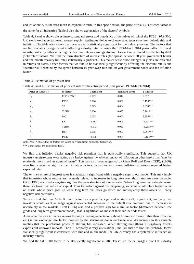
Table 4, Panel A shows the estimates, standard errors and t-statistics of the prices of risk of the FTSE, S&P 500,

UK stock exchange turnover, money supply, sterling/us dollar exchange rate, term structure, default risk and

inflation. The table also shows that these are all statistically significant for the industry sectors. The factors that

we find statistically significant in affecting industry returns during the 1993-March 2014 period affect firm and

industry value by either affecting the discount rate or earnings stream. Discount rates should be affected by debt

yield/return factors. We find the term structure of interest rates (the spread between 20 year government bonds

and one month treasury bill rate) statistically significant. This makes sense since changes in yields are reflected

in returns on assets. Other factors that we find to be statistically significant by affecting the discount rate is our

“default risk”; proxied by the spread between 10 year swap rate and 20 year government bonds and the inflation

factor.

Table 4. Estimation of prices of risk

Table 4 Panel A. Estimation of prices of risk for the entire period (time period 1993-March 2014)

Price of Risk ( ) of factor Coefficient Standard Error t-statistic

0 CONSTANT 0.087 0.017 0.517

1 FTSE 0.006 0.002 3.153***

2 SP 0.023 0.004 6.324***

3 TURN 0.220 0.037 5.981***

4 MO 0.003 0.000 5.856***

5 EX -0.017 0.003 -6.207***

6 TERM -0.173 0.033 -5.255***

7 DEF 0.035 0.009 3.991***

8 INFL -0.176 0.034 -5.164***

Note. Panel A shows that all factors are statistically significant during the full period.

*** significant at 1% confidence level.

We find that inflation carries negative risk premium that is statistically significant. This suggests that UK

industry assets/returns were acting as a hedge against the adverse impact of inflation on other assets that “may be

relatively more fixed in nominal terms”. This has also been suggested by Chen Roll and Ross (CRR), (1986),

who find a negative sign for their inflation factors. Industries with lower inflation exposures required higher

expected return.

The term structure of interest rates is statistically significant with a negative sign in our model. This may imply

that industries whose returns are inversely related to increases in long rates over short rates are more valuable.

CRR (1986) also find a negative sign for the term structure of interest rates. When long term real rates decrease,

there is a lower real return on capital. Thus to protect against this happening, someone would place higher value

on assets whose price goes up when long term real rates go down and subsequently these assets will carry

negative risk premiums.

We also find that our “default risk” factor has a positive sign and is statistically significant, implying that

investors would want to hedge against unexpected increases in the default risk premium due to increases in

uncertainty in the markets. CRR (1986) also find a positive sign for a similar factor (difference between low

grade and long term government bonds), that is significant on most of their sub-periods tested.

A variable that can influence returns through affecting expectations about future cash flows (other than inflation,

etc.) is our exchange rate factor, proxied by the sterling/us dollar exchange rate. An increase in this variable

implies that the purchasing power of sterling has increased. When sterling strengthens it negatively affects

exports but improves imports. The UK economy is very international; the fact that we find the exchange factor

statistically significant is consistent with this and in our model the UK currency has a systematic influence on

industry returns.

We find the S&P 500 factor to be statistically significant in UK. These two factors suggest that UK industry


118

returns are affected by the US stock market and the value of sterling in relation to the dollar; which is what we

have seen in practise throughout time.

A theoretical foundation for the signs of the factors has not been developed. A review of the literature in asset

pricing shows that in some cases different researchers find different signs for the same factor/proxy. A possible

explanation for this, which is not in the scope of this paper, is the use of different data sets.

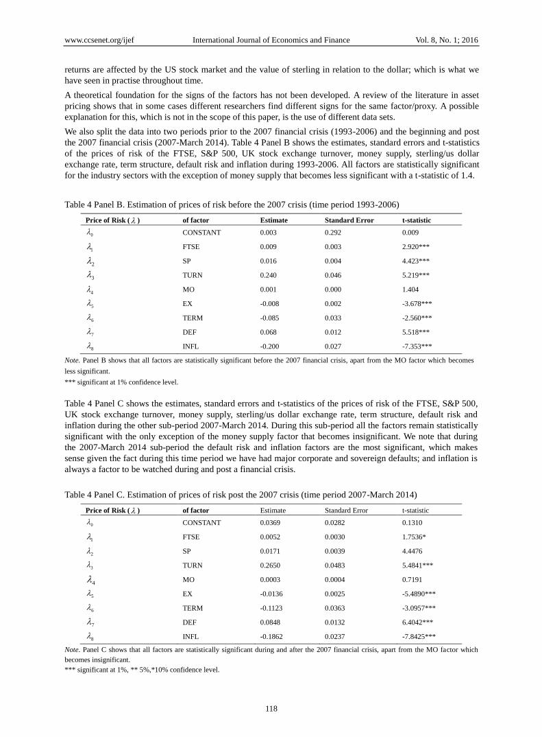
We also split the data into two periods prior to the 2007 financial crisis (1993-2006) and the beginning and post

the 2007 financial crisis (2007-March 2014). Table 4 Panel B shows the estimates, standard errors and t-statistics

of the prices of risk of the FTSE, S&P 500, UK stock exchange turnover, money supply, sterling/us dollar

exchange rate, term structure, default risk and inflation during 1993-2006. All factors are statistically significant

for the industry sectors with the exception of money supply that becomes less significant with a t-statistic of 1.4.

Table 4 Panel B. Estimation of prices of risk before the 2007 crisis (time period 1993-2006)

Price of Risk ( ) of factor Estimate Standard Error t-statistic

0 CONSTANT 0.003 0.292 0.009

1 FTSE 0.009 0.003 2.920***

2 SP 0.016 0.004 4.423***

3 TURN 0.240 0.046 5.219***

4 MO 0.001 0.000 1.404

5 EX -0.008 0.002 -3.678***

6 TERM -0.085 0.033 -2.560***

7 DEF 0.068 0.012 5.518***

8 INFL -0.200 0.027 -7.353***

Note. Panel B shows that all factors are statistically significant before the 2007 financial crisis, apart from the MO factor which becomes

less significant.

*** significant at 1% confidence level.

Table 4 Panel C shows the estimates, standard errors and t-statistics of the prices of risk of the FTSE, S&P 500,


inflation during the other sub-period 2007-March 2014. During this sub-period all the factors remain statistically

significant with the only exception of the money supply factor that becomes insignificant. We note that during

the 2007-March 2014 sub-period the default risk and inflation factors are the most significant, which makes

sense given the fact during this time period we have had major corporate and sovereign defaults; and inflation is

always a factor to be watched during and post a financial crisis.

Table 4 Panel C. Estimation of prices of risk post the 2007 crisis (time period 2007-March 2014)

Price of Risk ( ) of factor Estimate Standard Error t-statistic

0 CONSTANT 0.0369 0.0282 0.1310

1 FTSE 0.0052 0.0030 1.7536*

2 SP 0.0171 0.0039 4.4476

3 TURN 0.2650 0.0483 5.4841***

4 MO 0.0003 0.0004 0.7191

5 EX -0.0136 0.0025 -5.4890***

6 TERM -0.1123 0.0363 -3.0957***

7 DEF 0.0848 0.0132 6.4042***

8 INFL -0.1862 0.0237 -7.8425***

Note. Panel C shows that all factors are statistically significant during and after the 2007 financial crisis, apart from the MO factor which

becomes insignificant.

*** significant at 1%, ** 5%,*10% confidence level.


119

We find additional factors to the ones found significant by Chen Roll and Ross (CRR) (1986). Poon and Taylor

(1991), also suggest that probably other macroeconomic factors except from the CRR (1986) are at work in the

UK market. Our findings are not inconsistent with previous findings in the UK market. Antoniou, Garrett and

Priestley (1998) find unexpected inflation, money supply and the market portfolio to be significant for 138

securities traded on the London Stock exchange, from January 1980 to August 1993. Antoniou, Garrett and

Priestley (1998) in another study assessing the impact of exchange rate mechanism find inflation, money supply,

default risk, exchange rate and to a lesser extent the market portfolio significant for 69 companies from 1989 to

1993. Clare Priestley and Thomas (1997) also find a proxy for unexpected inflation, the market portfolio and

default risk to be priced for 15 stocks from 1978 to 1990.

5. Conditional and Unconditional Betas Estimation

Having identified our set of statistically significant macroeconomic factors using NLSUR described and

discussed in section 3 and 4, we estimate 1) unconditional-constant betas and (2) conditional time varying betas

for our factors.

In order to estimate the cost of equity capital as precise as possible we need precise estimates of exposure

coefficients for each of the factors. Estimates of the APM would be precise, provided that betas are constant over

time, however there is evidence that these vary over time. In order to examine this issue, we estimate full-period

constant-unconditional and time varying conditional betas.

5.1 Unconditional-Constant Betas Estimation

The constant-unconditional betas are the slopes of the regression of the individual industry return on the factors

throughout the period. During this period (1993-March 2014) the betas are assumed to be constant.

ittINFLtDEFtTERM

tEXCtMOtTUtSPtFTiINDUSTRYit

eINFLbDEFbTERMb

EXCbMObTUbSPbFTbR

(7a)

Consistent with the previous equations,INDUSTRYitR is the industry return i in month t ;

i a constant term;

INFLDEFTERMEXCMOTUSPFT bbbbbbbb ,,,,,,, are the betas of the return on FTSE, S&P 500, UK stock exchange

turnover, money supply, sterling/us dollar exchange rate, term structure, default risk and inflation (i.e. 𝑏𝑖𝑗 the

sensitivity of the industry return i to factor j ), ite is the zero mean error term.

The betas measure the average response of each industry to unanticipated changes in the respective economic

factors. Some industries have negative betas and tend to do worse than expected when a factor is greater than

expected. We find that in the constant beta model individual regressions of each industry onto the factors, for

some industries some factors are more significant than others and the sign of some factors varies from positive to

negative. This is not surprising as each industry has different sensitivity to different factors (Note 2).

Table 5 shows the adjusted R-squared of the regression of each industry return on the factors (to obtain the

unconditional-constant betas). The results indicate that the predictive ability of the constant beta model varies

from industry to industry. The average adjusted R-squared is approximately 43%. The tobacco industry has

lowest adjusted R-squared of approximately 12%, however as Table 1 shows there are only 2 firms included in

the tobacco index. The equity investment industry has the highest adjusted R-squared of 84.3%, as Table 1 shows

there are 177 firms included in this index. Elton, Gruber and Mei (1994) report adjusted R-squared in the range

of 16% to 40% of the regressions to obtain the betas of their APM.

Table 5. Unconditional-constant betas regression adjusted r-squared

Symbol Industry Adjusted R-squared

BANK FTSE ASX Banks Index 67.54%

MNG FTSE ASX Mining Index 48.78%

PHRM FTSE ASX Pharmaceuticals & Biotechnology 20.26%

SUPP FTSE ASX Support Services Index 59.95%

LIFE FTSE ASX Life Insurance Index 58.34%

TOBC FTSE ASX Tobacco Index 11.76%

BEVG FTSE ASX Beverages Index 32.09%

LEIS FTSE ASX Travel Leisure Index 57.85%

INVC FTSE ASX Investment Instruments 84.27%

MEDA FTSE ASX Media Index 56.36%


120

FOOD FTSE ASX Food Producers Index 28.78%

OTHR FTSE ASX Fin Services Index 65.14%

RETG FTSE ASX Gen Retailers Index 41.71%

AERO FTSE ASX Aerospace & Defence 45.54%

FDRT FTSE ASX Food Drug Retailers Index 18.65%

TELE FTSE ASX Fixed Line Telecommunications 36.92%

INSU FTSE ASX Nonlife Insurance Index 42.75%

ENGN FTSE ASX Industrial Engineering Index 57.04%

CONS FTSE ASX Construct Material Index 48.51%

INFT FTSE ASX Tech Hardware Index 24.72%

CHEM FTSE ASX Chemicals Index 49.51%

SOFT FTSE ASX Software & Computer Service 38.34%

ELTR FTSE ASX Electronic & Electrical Equipment 41.62%

HLTH FTSE ASX Health Care Equipment and Services 24.40%

PERC FTSE ASX Personal Goods Index 24.63%

AUTO FTSE ASX Automobiles Parts Index 40.80%

TRAN FTSE ASX Industrial Transportation Index 52.63%

HOUS FTSE ASX Leisure Goods Index 15.25%

AVERAGE 42.65%

5.2 Conditional Betas Estimation

Conditional betas, defined in this paper, incorporate not only time variation as a property, but also these betas are

conditioned to a set of information-instrumental variables, which reflect information in the market that investors

use.

Conditional beta estimation involves the following steps. Step 1, the estimation of rolling betas. Step 2, the use

of these rolling betas as dependent variable regressed on a set of instrumental variables. The fitted values from

this regression (the beta regressed on the instrumental variables) are defined as the conditional beta. Thus, in the

first step we incorporate the time variation property in the estimation of the conditional betas. The second step

incorporates the conditional property, since the time-varying betas are conditioned on a set of instrumental

variables that convey publicly available information.

Step 1: In order to document temporal variation in betas, we estimate rolling regressions using five years of past

returns, i.e., using a rolling window of 60 prior monthly returns. Thus the industry’s exposure to the

macroeconomic factors and the market index are estimated by regressing the industry return on the unanticipated

components of the factors, using time series regressions over an estimation period of 5 years, i.e., (60 months

rolling). The slope coefficients in the time-series regressions provide estimates of the betas. We use the five-year

period and update the estimates annually. For example, we run the following regression with the industry return

being the dependent variable on the factors, from 1993-1997 in order to obtain betas for 1998.

ittINFLtDEFtTERM

tEXCtMOtTUtSPtFTiINDUSTRYit

eINFLbDEFbTERMb

EXCbMObTUbSPbFTbR

(7b)

Consistent with the previous equations,INDUSTRYitR is the industry return i in month t ;

i a constant term;

INFLDEFTERMEXCMOTUSPFT bbbbbbbb ,,,,,,, are the betas of the return on unexpected FTSE, S&P 500, UK stock

exchange turnover, money supply, sterling/us dollar exchange rate, term structure, default risk and inflation (i.e.

𝑏𝑖𝑗 the sensitivity of the industry return i to factor j ), ite is the zero mean error term.

Thus the outcome of step 1 is a time-series (from 1998 to March 2014) of rolling betas for each factor. In step 2,

each beta is used as dependent variable regressed on a constant and a set of instrumental variables. The fitted

values from this regression are defined as the conditional betas. A conditional beta is defined as the beta

conditioned on a set of instrumental variables.

Hence having obtained a time series of rolling betas from 1998 to March 2014 for the return on FTSE, S&P 500,


inflation, we use the following model and run it for each factor 𝐽.

tttttjt eIFTITSIDIVITBb 141312110 1 (8)


121

Where 𝑏𝑗𝑡 represents the beta/sensitivity associated with each factor j , te is the residual,

0 is a constant and

𝛿1 to 𝛿4 are the coefficients of the instrumental variables 1111 ,,,1 tttt IFTITSIDIVITB ; the one month Treasury

bill rate, lagged one month, the dividend yield on FT all share price index, lagged one month, the term structure

of interest rates, lagged one month and the return on FT all share price index, lagged one month. These

instrumental variables are chosen because they summarise expectations in the economy that are related to the

prospects for stock returns, that is they have the ability to forecast asset returns. Short-term interest rates, for

example, have been prominent instruments in several studies (Note 3); their importance as instruments in tests of

asset pricing models stems from their relation with consumption, production and returns. The dividend yield has

also been examined and found to have predictive ability (Note 4).

To forecast the conditional betas we estimate conditional betas with an out-of-sample evaluation. We fit a model

in which the rolling beta is used as dependent variable regressed on a constant and a set of instrumental variables.

We use a holdout sample of 132 months where the out-of-sample evaluation is taking place. Using an initial

estimation period of 60 months from 1998-2002, we forecast the conditional betas for the next twelve months,

January-December 2003. Then the next twelve months are added to the estimation period to forecast the

conditional betas for the following twelve months, January-December 2004 (Note 5). The most statistically

significant instrumental variables (at the 1% level) are the term structure of interest rates lagged one month

(1tITS ) and dividend yield on FT all share price index lagged one month (

1tIDIV ). This is not surprising since

the tem structure of interest rates is very important in assessing overall economic growth and dividend yields are

a component of stock returns.

Table 6 reports the Adjusted R-squared of the regression of the rolling beta of each factor (FTSE, S&P 500, UK

stock exchange turnover, money supply, sterling/us dollar exchange rate, term structure, default risk and

inflation) used as dependent variable regressed on the instrumental variables for year 2013, for every industry

and averages. Due to vast amount of output from running conditional regressions we present results for 2013. All

the results can be provided upon request.

Table 6. Conditional betas regression adjusted r-squared

Industry/beta FTb SPb

TUb MOb

EXCb TERMb DEFb INFLb

AVERAGE adj. R2

for each industry

BANK 35.09% 68.16% 87.03% 38.65% 47.49% 80.25% 69.64% 35.38% 57.71%

MNG 62.61% 31.87% 2.65% 3.69% 66.37% 23.41% 66.70% 40.00% 37.16%

PHRM 4.33% 21.83% 2.48% 65.04% 64.79% 65.03% 22.96% 67.62% 39.26%

SUPP 51.82% 62.06% 58.80% 82.03% 23.30% 15.54% 80.42% 63.78% 54.72%

LIFE 47.03% 33.04% 47.74% 46.43% 20.04% 42.59% 80.13% 71.86% 48.61%

TOBC 61.27% 42.25% 43.25% 78.97% 39.94% 76.80% 38.77% 14.00% 49.41%

BEVG 32.28% 40.42% 58.97% 67.13% 43.72% 67.17% 54.17% 81.33% 55.65%

LEIS 6.82% 16.23% 62.29% 78.28% 23.36% 82.51% 86.93% 4.43% 45.11%

INVC 81.07% 22.09% 85.71% 48.51% 56.51% 70.85% 72.06% 43.38% 60.02%

MEDA 44.20% 52.53% 85.07% 64.78% 8.14% 81.37% 83.86% 24.49% 55.55%

FOOD 70.16% 71.59% 63.11% 80.37% 52.98% 66.97% 28.80% 71.23% 63.15%

OTHR 74.10% 36.58% 85.10% 15.53% 2.98% 35.90% 41.83% 34.93% 40.87%

RETG 78.38% 78.15% 60.67% 30.47% 73.06% 86.21% 62.90% 3.07% 59.11%

AERO 30.46% 6.05% 58.09% 79.39% 37.26% 45.57% 72.30% 35.62% 45.59%

FDRT 65.67% 61.82% 69.36% 32.21% 55.88% 51.77% 67.59% 7.75% 51.51%

TELE 14.82% 20.24% 51.39% 78.99% 26.44% 56.63% 5.21% 41.34% 36.88%

INSU 66.07% 45.35% 57.89% 8.09% 18.03% 82.55% 48.72% 75.57% 50.28%

ENGN 42.04% 48.01% 42.84% 45.13% 73.99% 51.26% 83.51% 78.26% 58.13%

CONS 37.61% 45.11% 39.86% 84.92% 62.62% 79.37% 74.51% 40.19% 58.02%

INFT 54.95% 20.29% 44.48% 72.24% 9.30% 29.69% 48.84% 52.07% 41.48%


122

CHEM 24.84% 29.51% 61.41% 66.25% 54.92% 86.12% 57.59% 64.71% 55.67%

SOFT 70.97% 29.44% 86.45% 70.58% 27.24% 79.10% 42.32% 55.20% 57.66%

ELTR 58.78% 60.04% 86.75% 12.97% 36.21% 41.25% 72.80% 45.16% 51.74%

HLTH 70.21% 63.94% 45.06% 9.51% 16.76% 55.82% 79.29% 21.50% 45.26%

PERC 69.40% 65.82% 85.79% 86.62% 7.14% 60.24% 62.63% 66.15% 62.97%

AUTO 35.23% 27.03% 3.26% 64.06% 35.35% 64.47% 75.02% 52.88% 44.66%

TRAN 53.10% 27.07% 34.21% 60.28% 38.39% 56.16% 39.61% 14.92% 40.47%

HOUS 42.37% 55.32% 68.65% 63.92% 57.62% 27.90% 66.70% 33.91% 52.05%

AVERAGE adj. R2

for each beta 49.49% 42.21% 56.37% 54.82% 38.57% 59.38% 60.21% 44.31%

For example Table 6, row 1, reports that for the banking industry (BANK) the rolling beta (TUb ) of the stock

exchange turnover when regressed on the instrumental variables, has the highest adjusted R squared of 87.03%,

amongst the other rolling betas within that industry.

Looking at each element of the last column we see the average predictive ability of the conditional regressions of

all factors’ rolling betas per industry (average adjusted R-squared for all rolling betas FTb ,

SPb ,TUb ,

MOb ,EXCb ,

TERMb ,

DEFb ,INFLb ) for each industry; the highest adjusted R-squared is 63.15% for the food industry (FOOD) and the

lowest is 37.12% for the mining industry (MNG). Ferson and Harvey (1991) report adjusted R-squared for the

conditional regressions (i.e. 5 year rolling beta on the lagged instruments) in the range of 20%.

Looking at Table 6, bottom row per column, we see the average adjusted R-squared for all the industries per beta

(of the regression of the rolling betas of each factor regressed on a constant and the set of instrumental variables).

This average adjusted R-squared varies from the highest adjusted R-squared of 60.21% for the rolling beta (DEFb )

of the default risk factor to the lowest of 42.21% for the rolling beta (SPb ) of the S&P factor.

6. The CAPM

We obtain CAPM estimates of the UK industry cost of equity capital for the full-period (1993-March 2014).

Using NLSUR we obtain an estimate of the market portfolio price of risk that is equal across every industry and

different market betas for each industry.

Table 7 shows the market beta estimates for each industry based on the CAPM. The standard error and t-statistic

are also reported.

Table 7. Market beta

Symbol Industry Market Beta Standard Error t-statistic

BANK FTSE ASX Banks Index 1.02 0.033 30.464

MNG FTSE ASX Mining Index 1.10 0.049 22.481

PHRM FTSE ASX Pharmaceuticals & Biotechnology 0.88 0.036 24.455

SUPP FTSE ASX Support Services Index 1.01 0.024 41.543

LIFE FTSE ASX Life Insurance Index 1.06 0.037 28.448

TOBC FTSE ASX Tobacco Index 0.89 0.046 19.212

BEVG FTSE ASX Beverages Index 0.94 0.031 30.643

LEIS FTSE ASX Travel Leisure Index 1.02 0.026 38.837

INVC FTSE ASX Investment Instruments 1.02 0.015 68.292

MEDA FTSE ASX Media Index 1.08 0.031 34.877

FOOD FTSE ASX Food Producers Index 0.94 0.031 29.971

OTHR FTSE ASX Fin Services Index 1.02 0.032 31.812

RETG FTSE ASX Gen Retailers Index 1.09 0.032 34.374

AERO FTSE ASX Aerospace & Defence 0.99 0.035 28.120

FDRT FTSE ASX Food Drug Retailers Index 0.87 0.037 23.421

TELE FTSE ASX Fixed Line Telecommunications 1.01 0.044 23.114

INSU FTSE ASX Nonlife Insurance Index 1.07 0.037 29.120


123

ENGN FTSE ASX Industrial Engineering Index 1.05 0.034 30.312

CONS FTSE ASX Construct Material Index 1.05 0.034 30.902

INFT FTSE ASX Tech Hardware Index 1.19 0.084 14.051

CHEM FTSE ASX Chemicals Index 0.98 0.034 28.926

SOFT FTSE ASX Software & Computer Service 1.12 0.054 20.622

ELTR FTSE ASX Electronic & Electrical Equipment 1.04 0.060 17.397

HLTH FTSE ASX Health Care Equipment and Services 0.91 0.037 24.843

PERC FTSE ASX Personal Goods Index 0.94 0.045 20.996

AUTO FTSE ASX Automobiles Parts Index 0.97 0.057 16.966

TRAN FTSE ASX Industrial Transportation Index 0.99 0.029 33.457

HOUS FTSE ASX Leisure Goods Index 1.04 0.055 18.844

The market betas are statistically significant for all industries. We find, for example, the banking sector to have a

beta of 1.02, life insurance of 1.06, the pharmaceuticals 0.88, tobacco 0.89, beverages 0.94, food producers 0.94,

general retailers 1.09. Fama and French (1997) find broadly similar betas for similar industry indices in the US

market. They report the following betas: for the banking sector 1.09, pharmaceuticals 0.92, insurance 1.01,

tobacco 0.8, beverages 0.92, food producers 0.87, and general retailers. Bloomberg reports similar betas in the

UK.

7. Cost of Equity Capital

Having estimated the prices of risk of our macroeconomic factor model; the constant betas for the unconditional

APM; the conditional-time varying betas for the conditional APM; and the common CAPM, we incorporate

these estimates to calculate the cost of equity capital.

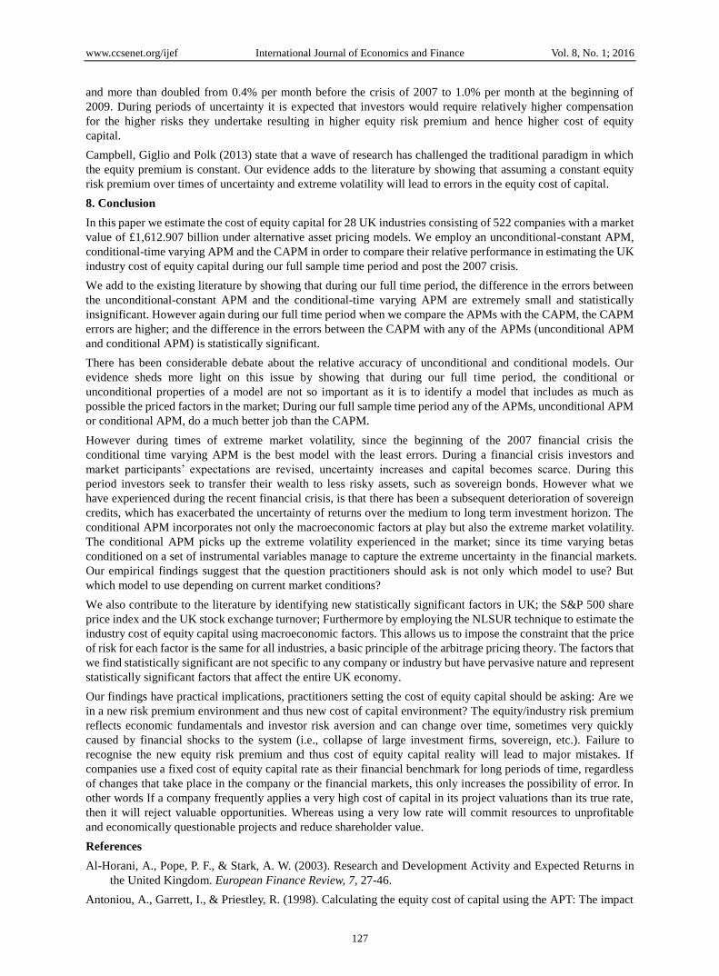
Figure 1 shows the CAPM, unconditional-constant APM and conditional-time varying APM weighted average

cost of equity capital for all industries. The weighted average cost of equity capital from 2003 until March 2014

estimated by the CAPM is 13.2%, 9.1% by the unconditional-constant APM and 10.1% by the conditional-time

varying APM. The conditional-time varying APM varies from 5%-6% just before the 2007 crisis to over 16%

post the crisis; starting to gradually increase just after the financial crisis. It seems that the conditional APM

picks up the fact that high expected returns are required in recessions by investors to make up for the additional

risk. Goldenberg and Robin (1991), find a cost of equity capital for their portfolio of US electric utilities of 17%

using macroeconomic factor APM, whereas with the statistical factor APM and the CAPM they find it to be at

15.35% and 11.56% respectively.

Figure 1. Industry Cost of Equity Capital (CEC)

Tables 8, 9, 10 and 11 show the errors of the cost of equity capital for each model and whether the difference in

the errors between the competing models is statistically significant. In order to evaluate the comparative

0.0%

2.0%

4.0%

6.0%

8.0%

10.0%

12.0%

14.0%

16.0%

18.0%

20.0%

2003 2004 2005 2006 2007 2008 2009 2010 2011 2012 2013 2014

CAPM CEC

Unconditional-ConstantAPM CEC

Conditional-time varyingAPM CEC


124

performance of the alternative models estimated, we use the Mean Square Error (MSE). In general, tests

employed to compare performance of models are unique and no single test is superior to all others; all have

advantages and disadvantages. In the literature and in practise the Mean Square Error (MSE) test has been

frequently used. The MSE is a summary measure and provides for a quadratic loss function as it squares and

subsequently averages the various errors.

n

t

t

vn

eMSE

1

2

(9)

Where et is the difference between the model’s estimates and the actual industry returns, n is the number of

observations and the number of independent variables.

We report weighted average MSE for each model for i) our reduced full period (2003-March 2014) (the full

period is reduced due to the fact that we lose some observations due to running conditional regressions for the

conditional APM (Note 6) and (ii) during and after the 2007 financial crisis (2007 until March 2014). The

objective is to investigate the performance of the models not only during our full sample time period but also

during and post a financial crisis.

Table 8 shows the MSE for each industry and the weighted average MSE for the reduced full time period

(2003-March 2014). The weighted average MSE for the unconditional, conditional beta APM and the CAPM is

0.009, 0.0011 and 0.024 respectively. We notice that the differences in the MSE between the two APMs are very

small. So we test whether the difference between the MSE of the conditional and the unconditional APM is

statistically significant with a t-test. Table 9 shows that the p-value of 0.315 is greater than the critical value of

0.05, indicating that the difference in the MSE of the two APMs is statistically insignificant; implying that the

errors of the two APMs are more or less the same. On the other hand when we test whether the difference

between the CAPM MSE and the unconditional APM MSE is statistically significant, we find a p-value of 0.00,

indicating that this difference in the MSE is statistically significant. The CAPM errors are higher and

significantly different from the errors of the unconditional APM. Similarly we find a p-value of 0.00, when we

test the statistical significance of the difference in the CAPM MSE and the conditional APM MSE, showing that

the difference in the MSE is statistically significant. The CAPM errors are higher and significantly different from

the errors of the conditional APM. These results imply that during the full period it is not so important whether

one uses the unconditional or the conditional APM as the difference in their MSEs is statistically insignificant.

On the contrary the difference in the MSE of the CAPM with any of the APMs MSE is statistically significant.

The MSE of the CAPM is higher compared to any of the APMs. The full period results imply that there is not so

much difference in the errors of the cost of equity capital estimated between unconditional and conditional beta

model as there is between the CAPM and the APM.

Our evidence that the APM is much better than the CAPM is consistent with US evidence. Pettway and Jordan

(1987) in their comparison of the relative efficiency of the CAPM and APT, using weekly data on electric

utilities, find that the APM provides better estimates of equity returns than the CAPM. However our study

extends the existing literature by showing that both unconditional and conditional versions of the APM are better

than the CAPM.

Table 8. Mean Square Error (MSE)-reduced full time period (2003-March 2014)

Symbol Industry CAPM APM-Unconditional APM-Conditional



PHRM FTSE ASX Pharmaceuticals & Biotechnology 0.0019 0.0004 0.0005

SUPP FTSE ASX Support Services Index 0.0021 0.0006 0.0006

LIFE FTSE ASX Life Insurance Index 0.0028 0.0014 0.0016



LEIS FTSE ASX Travel Leisure Index 0.0021 0.0005 0.0007

INVC FTSE ASX Investment Instruments 0.0020 0.0006 0.0007


FOOD FTSE ASX Food Producers Index 0.0020 0.0004 0.0006

OTHR FTSE ASX Fin Services Index 0.0021 0.0010 0.0010

RETG FTSE ASX Gen Retailers Index 0.0027 0.0007 0.0007


125

AERO FTSE ASX Aerospace & Defence 0.0022 0.0008 0.0011

FDRT FTSE ASX Food Drug Retailers Index 0.0020 0.0005 0.0005

TELE FTSE ASX Fixed Line Telecommunications 0.0026 0.0014 0.0014

INSU FTSE ASX Nonlife Insurance Index 0.0025 0.0006 0.0008

ENGN FTSE ASX Industrial Engineering Index 0.0024 0.0009 0.0014

CONS FTSE ASX Construct Material Index 0.0024 0.0008 0.0012

INFT FTSE ASX Tech Hardware Index 0.0037 0.0026 0.0049


SOFT FTSE ASX Software & Computer Service 0.0028 0.0016 0.0017

ELTR FTSE ASX Electronic & Electrical Equipment 0.0028 0.0025 0.0035

HLTH FTSE ASX Health Care Equipment & Services 0.0022 0.0007 0.0008

PERC FTSE ASX Personal Goods Index 0.0024 0.0011 0.0009

AUTO FTSE ASX Automobiles Parts Index 0.0031 0.0026 0.0030

TRAN FTSE ASX Industrial Transportation Index 0.0021 0.0007 0.0008

HOUS FTSE ASX Leisure Goods Index 0.0035 0.0017 0.0019

AVERAGE

0.0024 0.0009 0.0011

Note. The period is reduced starting from 2003 as we lose observations by running conditional regressions for the conditional APM.

n

t

t

vn

eMSE

1

2 Where te is the difference between the model estimates and the actual industry returns, is the number of observations

and the number of independent variables.

Table 9. MSE T-test –reduced full time period (2003-March 2014)

p-value testing statistical significance of the difference in MSE of

the Unconditional and Conditional APM

0.315

p-value>0.05; the difference in the MSE is

statistically insignificant


the CAPM and Conditional APM

0.000

p-value<0.05; the difference in the MSE is

statistically significant at the 5% level


the CAPM and Unconditional APM

0.000



Table 10 shows the MSE for each industry and the weighted average MSE from 2007- March 2014 for all

models. We also test the statistical significance of the difference in the MSEs between the competing models

with a t-test in Table 11.

Table 10. Mean Square Error (MSE)-time period (2007-March 2014)

MSE Industry CAPM APT-Unconditional APT-Conditional



PHRM FTSE ASX Pharm & Biotech 0.0026 0.0010 0.0004

SUPP FTSE ASX Support Srvcs 0.0028 0.0013 0.0007

LIFE FTSE ASX Life Insurance 0.0032 0.0028 0.0015



LEIS FTSE ASX Travel Leisure 0.0030 0.0014 0.0006

INVC FTSE ASX Eqy Invst Instr 0.0026 0.0015 0.0008


FOOD FTSE ASX Food Producers 0.0028 0.0010 0.0006

OTHR FTSE ASX Fin Services 0.0027 0.0025 0.0013

RETG FTSE ASX Gen Retailers 0.0038 0.0015 0.0008

AERO FTSE ASX Aero & Defense 0.0027 0.0018 0.0010

FDRT FTSE ASX Food Drug Retl 0.0027 0.0011 0.0006

TELE FTSE ASX Fixed Line Tele 0.0033 0.0035 0.0014

INSU FTSE ASX Nonlife Insur 0.0031 0.0019 0.0008


126

ENGN FTSE ASX Indust Engineer 0.0031 0.0022 0.0015

CONS FTSE ASX Construct Mater 0.0034 0.0017 0.0012

INFT FTSE ASX Tech Hardware 0.0036 0.0096 0.0050


SOFT FTSE ASX Sftwr Comp Srvs 0.0030 0.0054 0.0013

ELTR FTSE ASX Elect/Ele Equip 0.0030 0.0068 0.0046

HLTH FTSE ASX Health Care Eqp 0.0029 0.0014 0.0008

PERC FTSE ASX Personal Goods 0.0035 0.0024 0.0012

AUTO FTSE ASX Automobiles Prt 0.0041 0.0051 0.0040

TRAN FTSE ASX Indust Transprt 0.0030 0.0015 0.0009

HOUS FTSE ASX Leisure Goods 0.0050 0.0033 0.0026

AVERAGE 0.0031 0.0023 0.0012

Note.

n

t

t

vn

eMSE

1

2

Where te is the difference between the model estimates and the actual industry returns, is the number of

observations and the number of independent variables.

Table 11 shows that the p-value of 0.008 is lower than the critical value of 0.05, indicating that the difference in

the MSE of the unconditional and conditional APM is statistically significant. During and post the period of

financial crisis the conditional APM with a MSE of 0.0012 provides more accurate estimates compared to the

unconditional model (MSE 0.0023).

Table 11 reports a p-value of 0.172 when we test the difference in the errors between the unconditional APM and

the CAPM from 2007 onwards. Indicating that the difference in the MSE between the CAPM and unconditional

APM is statistically insignificant. Further the difference in the errors between the conditional APM and the

CAPM is statistically significant with a p-value of 0.00.

Table 11. MSE T-test time period (2007-March 2014)

p-value testing statistical significance of the difference in MSE

of the Unconditional and Conditional APM

0.008



p-value testing statistical significance of the difference in MSE

of the CAPM and Conditional APM

0.000



p-value testing statistical significance of the difference in the

MSE of the CAPM and Unconditional APM

0.172

p-value>0.05; the difference in the MSE is

statistically insignificant

During and post the financial crisis of 2007, we find that the conditional APM with a MSE of 0.0012 provides

more accurate estimates compared to the unconditional APM (MSE 0.0023) and the CAPM (MSE 0.0031) for all

industries. The conditional APM performs better from the models tested during the period of crisis. During the

2007 crisis there was a lot of volatility in the marketplace. In order to assess whether indeed the market volatility

is a significant variable in the conditional cost of equity capital during 2007 to March 2014, we regress the

conditional cost of equity capital on to a constant and the FTSE volatility index. We find the FTSE volatility

index to be statistically significant at the 1% level with a t-statistic of 6.363 and a regression adjusted R-squared

of 44%.

During the period that the conditional APM performs best we have had major disruptions in financial markets.

From 2007 we had major defaults in the mortgage market for subprime borrowers. Many banks and firms

suffered losses of hundreds of billions. Credit became much harder to obtain and much more expensive. As a

result lending declined, consumption and investment fell causing further sharp contraction in the economy. The

uncertainty in the economy went on with major failures of high profile firms.

The economic repercussions of our results indicate that during the period of severe economic downturn with

general loss of confidence in the financial markets the conditional APM with time varying betas and conditioned

on the set of instrumental variables used by investors is able to pick up the extreme market volatility in its betas

for each factor. As a consequence produces much better estimates. The conditional APM has a weighted average

cost of equity capital for all industries of 14.3% from 2007 to March 2014, while the unconditional APM cost of

equity capital for the same period is 10.8%. The average risk premium for the conditional APM varies per month


127

and more than doubled from 0.4% per month before the crisis of 2007 to 1.0% per month at the beginning of

2009. During periods of uncertainty it is expected that investors would require relatively higher compensation

for the higher risks they undertake resulting in higher equity risk premium and hence higher cost of equity

capital.

Campbell, Giglio and Polk (2013) state that a wave of research has challenged the traditional paradigm in which

the equity premium is constant. Our evidence adds to the literature by showing that assuming a constant equity

risk premium over times of uncertainty and extreme volatility will lead to errors in the equity cost of capital.

8. Conclusion

In this paper we estimate the cost of equity capital for 28 UK industries consisting of 522 companies with a market

value of £1,612.907 billion under alternative asset pricing models. We employ an unconditional-constant APM,

conditional-time varying APM and the CAPM in order to compare their relative performance in estimating the UK

industry cost of equity capital during our full sample time period and post the 2007 crisis.

We add to the existing literature by showing that during our full time period, the difference in the errors between

the unconditional-constant APM and the conditional-time varying APM are extremely small and statistically

insignificant. However again during our full time period when we compare the APMs with the CAPM, the CAPM

errors are higher; and the difference in the errors between the CAPM with any of the APMs (unconditional APM

and conditional APM) is statistically significant.

There has been considerable debate about the relative accuracy of unconditional and conditional models. Our

evidence sheds more light on this issue by showing that during our full time period, the conditional or

unconditional properties of a model are not so important as it is to identify a model that includes as much as

possible the priced factors in the market; During our full sample time period any of the APMs, unconditional APM

or conditional APM, do a much better job than the CAPM.

However during times of extreme market volatility, since the beginning of the 2007 financial crisis the

conditional time varying APM is the best model with the least errors. During a financial crisis investors and

market participants’ expectations are revised, uncertainty increases and capital becomes scarce. During this

period investors seek to transfer their wealth to less risky assets, such as sovereign bonds. However what we

have experienced during the recent financial crisis, is that there has been a subsequent deterioration of sovereign

credits, which has exacerbated the uncertainty of returns over the medium to long term investment horizon. The

conditional APM incorporates not only the macroeconomic factors at play but also the extreme market volatility.

The conditional APM picks up the extreme volatility experienced in the market; since its time varying betas

conditioned on a set of instrumental variables manage to capture the extreme uncertainty in the financial markets.

Our empirical findings suggest that the question practitioners should ask is not only which model to use? But

which model to use depending on current market conditions?

We also contribute to the literature by identifying new statistically significant factors in UK; the S&P 500 share

price index and the UK stock exchange turnover; Furthermore by employing the NLSUR technique to estimate the

industry cost of equity capital using macroeconomic factors. This allows us to impose the constraint that the price

of risk for each factor is the same for all industries, a basic principle of the arbitrage pricing theory. The factors that

we find statistically significant are not specific to any company or industry but have pervasive nature and represent

statistically significant factors that affect the entire UK economy.

Our findings have practical implications, practitioners setting the cost of equity capital should be asking: Are we

in a new risk premium environment and thus new cost of capital environment? The equity/industry risk premium

reflects economic fundamentals and investor risk aversion and can change over time, sometimes very quickly

caused by financial shocks to the system (i.e., collapse of large investment firms, sovereign, etc.). Failure to

recognise the new equity risk premium and thus cost of equity capital reality will lead to major mistakes. If

companies use a fixed cost of equity capital rate as their financial benchmark for long periods of time, regardless

of changes that take place in the company or the financial markets, this only increases the possibility of error. In

other words If a company frequently applies a very high cost of capital in its project valuations than its true rate,

then it will reject valuable opportunities. Whereas using a very low rate will commit resources to unprofitable

and economically questionable projects and reduce shareholder value.

References

Al-Horani, A., Pope, P. F., & Stark, A. W. (2003). Research and Development Activity and Expected Returns in

the United Kingdom. European Finance Review, 7, 27-46.

Antoniou, A., Garrett, I., & Priestley, R. (1998). Calculating the equity cost of capital using the APT: The impact


128

of the ERM. Journal of International Money and Finance, 17, 949-965.

http://dx.doi.org/10.1016/S0261-5606(98)00036-9

Antoniou, A., Garrett, I., & Priestley, R. (1998). Macroeconomic variables as common pervasive risk factors and

the empirical content of the arbitrage pricing theory. Journal of Empirical Finance, 5, 221-240.

http://dx.doi.org/10.1016/S0927-5398(97)00019-4

Bansal, R., & Yaron, A. (2004). Risks for the long run: A potential resolution of asset pricing puzzles. Journal of

Finance, 59, 1481-1509. http://dx.doi.org/10.1111/j.1540-6261.2004.00670.x

Bower, D. H., Bower, R. S., & Logue, D. E. (1984). Arbitrage pricing theory and utility stock returns. Journal of

Finance, 39, 1041-1054. http://dx.doi.org/10.1111/j.1540-6261.1984.tb03891.x

Cahart, M. (1997). On Persistence in Mutual Fund Performance. Journal of Finance, 52, 57-82.

Campbell, J. Y., Giglio, S., & Polk, C. (2013). Hard Times. Review of Asset Pricing Studies, 3, 95-132.

http://dx.doi.org/10.1093/rapstu/ras026

Campbell, J. Y. (1986). Stock returns and the term structure. Journal of Financial Economics, 18, 374-400.

http://dx.doi.org/10.1016/0304-405X(87)90045-6

Campbell, J. Y., & Hamao, Y. (1992). Predictable stock returns in the U.S. and Japan: A study of long-term

integration. Journal of Finance, 47, 43-72.

Campbell, J. Y., & Shiller, R. (1988). Stock prices, earnings and expected dividends. Journal of Finance, 43,

661-676. http://dx.doi.org/10.1111/j.1540-6261.1988.tb04598.x

Chen, N. F., Roll, R., & Ross, S. A. (1986). Economic forces and the stock market. Journal of Business, 59,

383-403. http://dx.doi.org/10.1086/296344

Claire, A. D., Priestley, R., & Thomas, S. H. (1998). Reports of beta’s death are premature: Evidence from the

UK. Journal of Banking and Finance, 22, 1207-1229. http://dx.doi.org/10.1016/S0378-4266(98)00050-8

Claire, A. D., Priestley, R., & Thomas, S. H. (1997). The robustness of the APT to alternative estimators. Journal

of Business Finance & Accounting, 24, 645-654. http://dx.doi.org/10.1111/1468-5957.00126

Cooper, I., & Priestley, R. (2013). The World Business Cycle and Expected Returns. Review of Finance, 17,

1029-1064. http://dx.doi.org/10.1093/rof/rfs014

Elton, E. J., Gruber, M. J., & Blake, C. R. (2012). An Examination of Mutual Fund Timing Ability Using

Monthly Holdings Data. Review of Finance, 16, 619-645. http://dx.doi.org/10.1093/rof/rfr007

Elton, E. J., Gruber, M. J., & Mei, J. (1994). Cost of equity using arbitrage pricing theory: A case study of nine

New York utilities. Financial Markets, Institutions & Instruments, 3, 45-64.

Fama E. F., & Schwert. (1977). Asset returns and inflation. Journal of Financial Economics, 5, 115-146.

http://dx.doi.org/10.1016/0304-405X(77)90014-9

Fama, E. F., & French, K. R. (1988). Dividend yields and expected stock returns. Journal of Financial

Economics, 22, 3-25. http://dx.doi.org/10.1016/0304-405X(88)90020-7

Fama, E. F., & French, K. R. (1992a). Common risk factors in the returns on stocks and bonds. Journal of

Financial Economics, 36, 1-55. http://dx.doi.org/10.1016/0304-405X(93)90023-5

Fama, E. F., & French, K. R. (1992b). The cross-section of expected stock returns. Journal of Finance, 47,

427-465. http://dx.doi.org/10.1111/j.1540-6261.1992.tb04398.x

Fama, E. F., & French, K. R. (1995). Size and Book-to-Market Factors in Earnings and Returns. Journal of


Fama, E. F., & French, K. R. (1996). Multifactor Explanations of Asset Pricing Anomalies. Journal of Finance,

50, 131-155. http://dx.doi.org/10.1111/j.1540-6261.1996.tb05202.x

Fama, E. F., & French, K. R. (1997). Industry costs of equity. Journal of Financial Economics, 43, 153-193.

http://dx.doi.org/10.1016/S0304-405X(96)00896-3

Fama, E. F., & French, K. R. (2006). Profitability, investment, and average returns. Journal of Financial

Economics, 82, 491-518. http://dx.doi.org/10.1016/j.jfineco.2005.09.009

Fama, E. F., & French, K. R. (2008). Dissecting anomalies. Journal of Finance, 63, 1653-1678.

Fama, E. F., & French, K. R. (2012). Size, value, and momentum in international stock returns. Journal of


129

Financial Economics, 105, 457-472.

Fama, E. F., & MacBeth, J. D. (1971). Risk, return and equilibrium: Empirical tests. Journal of Political

Economy, 71, 607-635. http://dx.doi.org/10.1086/260061

Ferson, W. E. (1989). Changes in expected security returns, risk and the level of interest rates. Journal of


Ferson, W. E., & Harvey, C. R. (1991). The variation of economic risk premiums. Journal of Political Economy,

99, 385-415. http://dx.doi.org/10.1086/261755

Ferson, W. E., & Harvey, C. (1999). Conditioning variables and the cross-section of stock returns. Journal of

Finance, 53, 407-432. http://dx.doi.org/10.1111/0022-1082.00148

Ferson, W. E., & Harvey, C. R. (1993). The risk and predictability of international equity markets. Review of

Financial Studies, 6, 527-566.

Ghysels, E. (1998). On stable factor structures in the pricing of risk: Do time varying betas help or hurt? Journal

of Finance, 53, 549-574. http://dx.doi.org/10.1111/0022-1082.224803

Goldenberg, D. H., & Robin, A. (1991). The arbitrage pricing theory and cost of capital estimation: The case of

electric utilities. The Journal of Financial Research, 45, 181-196.

Gregory, A., & Michou, M. (2009). Industry Cost of Equity Capital: UK Evidence. Journal of Business Finance

and Accounting, 36, 679-704. http://dx.doi.org/10.1111/j.1468-5957.2009.02135.x

Harvey, C. (1991). The world price of covariance risk. Journal of Finance, 46, 111-158.

http://dx.doi.org/10.1111/j.1540-6261.1991.tb03747.x

Lewellen, J., & Nagel, S. (2006). The conditional CAPM does not explain asset-pricing anomalies. Journal of

Financial Economics, 82, 289-314. http://dx.doi.org/10.1016/j.jfineco.2005.05.012

Lintner, J. (1965). The valuation of risk assets and the selection of risky investments in stock portfolios and

capital budgets. Review of Economic Statistics, 47, 13-37. http://dx.doi.org/10.2307/1924119

McElroy, M. B., & Burmeister, E. (1988). Arbitrage pricing theory as a restricted non-linear multivariate

regression model. Journal of Business & Economic Statistics, 6, 29-42.

Pettway, R. H., & Jordan, B. D. (1987). APT vs. CAPM estimates of the return generating function parameters

for regulated public utilities. Journal of Financial Research, 10, 227-238.

http://dx.doi.org/10.1111/j.1475-6803.1987.tb00493.x

Poon, S., & Taylor, S. J. (1991). Macroeconomic factors and the UK stock market. Journal of Business Finance

and Accounting, 18, 619-636. http://dx.doi.org/10.1111/j.1468-5957.1991.tb00229.x

Roll, R., & Ross, S. (1980). An empirical examination of the arbitrage pricing theory. Journal of Finance, 35,

1073-1103.

Roll, R., & Ross, S. (1983). Regulation, the capital asset pricing model and the arbitrage pricing theory. Public

Utilities Forum, 111, 22-28.

Roll, R., & Ross, S. (1984). A critical re-examination of the empirical evidence on the arbitrage pricing theory: A

reply. Journal of Finance, 39, 347-350.

Ross, S. (1976). The arbitrage pricing theory of capital asset pricing. Journal of Economic Theory, 13, 341-360.

http://dx.doi.org/10.1016/0022-0531(76)90046-6

Rozeff, M. (1984). Dividend yields are equity risk premiums. Journal of Portfolio Management, 11, 68-75.

Schink, G. R., & Bower, R. S. (1994). Application of the Fama-French model to utility stocks. Financial Markets,

Institutions & Instruments, 3, 56-78. http://dx.doi.org/10.3905/jpm.1984.408980

Sharpe, W. F. (1964). Capital asset prices: A theory of market equilibrium under conditions of risk. Journal of

Finance, 19, 425-442. http://dx.doi.org/10.2307/2977928

Shiller, R. J. (1984). Stock prices and social dynamics, Brooking Papers Economic Activity, 2, 457-510.

http://dx.doi.org/10.2307/2534436

Notes

Note 1. Where log return is: log 𝑉𝑎𝑟𝑖𝑎𝑏𝑙𝑒 𝑡 − 𝑙𝑜𝑔𝑉𝑎𝑟𝑖𝑎𝑏𝑙𝑒𝑡−1


130

Note 2. Due to the large output of results, for space considerations the regressions of the individual industry

return on the factors are not included in this paper. However they are available upon request.

Note 3. See for example, Ferson and Harvey (1991, 1993, 1999), Ferson and Korajczyk (1995), Ferson and

Schadt (1996), Ghysels (1998).

Note 4. Harvey (1991), Campbell and Hamao (1992), Rozeff (1984), Shiller (1984), Campbell and Shiller (1988),

Fama and French (1988), Bansal and Yaron (2004).

Note 5. Carrying out this exercise generates significant amount of output. For space considerations these

regressions are not included in this paper. However all results can be provided upon request.

Note 6. Please see section 5.2 Conditional Betas Estimation for more information.

Copyrights

Copyright for this article is retained by the author(s), with first publication rights granted to the journal.

This is an open-access article distributed under the terms and conditions of the Creative Commons Attribution

license (http://creativecommons.org/licenses/by/3.0/).

Alternative Estimating Methodologies of the UK Industry ...

Documents

Transcript of Alternative Estimating Methodologies of the UK Industry ...