ALMA MATER STUDIORUM- UNIVERSITA’ DI BOLOGNA Modelling ...
112
ALMA MATER STUDIORUM- UNIVERSITA’ DI BOLOGNA __________________________________________ Modelling, Simulation and Optimization of Maintenance Considerations on Condition Based Maintenance A dissertation submitted to the BUSINESS ORGANIZATION DEPARTMENT VIGO for the degree of Doctor of Industrial Engineering presented by GIOVANNI SCAGLIOSO accepted on the recommendation of Prof. Dr. Ana M.Mejìas Prof.Dr. Juan E. Pardo Prof.Dr. Emilio Ferrari 2014/2015 Session III
Transcript of ALMA MATER STUDIORUM- UNIVERSITA’ DI BOLOGNA Modelling ...

ALMA MATER STUDIORUM-
UNIVERSITA’ DI BOLOGNA
__________________________________________
Modelling, Simulation and
Optimization of Maintenance
Considerations on Condition Based Maintenance
A dissertation submitted to the
BUSINESS ORGANIZATION DEPARTMENT
VIGO
for the degree of
Doctor of Industrial Engineering
presented by
GIOVANNI SCAGLIOSO
accepted on the recommendation of
Prof. Dr. Ana M.Mejìas
Prof.Dr. Juan E. Pardo
Prof.Dr. Emilio Ferrari
2014/2015
Session III


i

ii

iii
ACKNOWLEDGMENTS
This report was made possible by a project of the Management
Department of University of Vigo.
I would like to thank you my doctoral supervisors first, Prof. Dr.
Juan E. Pardo and Prof. Dr. Ana M. Majìas for their support and
advice they have given me.
I really appreciated the fruitful dialogues, the inspiring exchange,
the constructive criticism concerning my work and the very
efficient collaboration.
My special thanks are extended to the whole team of the OSIG
research group, for their funding, support and their helpfulness
in every phase of my work.
I am grateful for having had access to any information and the
possibility to work in a well organized and equipped
environment. Finally, I would like to extend my gratitude to the
many people who helped to bring this research project to
fruition.

iv
ABSTRACT
Globalization has increased the pressure on organizations and
companies to operate in the most efficient and economic way.
This tendency promotes that companies concentrate more and
more on their core businesses, outsource less profitable
departments and services to reduce costs. By contrast to earlier
times, companies are highly specialized and have a low real net
output ratio. For being able to provide the consumers with the
right products, those companies have to collaborate with other
suppliers and form large supply chains. An effect of large supply
chains is the deficiency of high stocks and stockholding costs.
This fact has lead to the rapid spread of Just-in-Time logistic
concepts aimed minimizing stock by simultaneous high
availability of products. Those concurring goals, minimizing stock
by simultaneous high product availability, claim for high
availability of the production systems in the way that an
incoming order can immediately processed.
Besides of design aspects and the quality of the production
system, maintenance has a strong impact on production system
availability.
In the last decades, there has been many attempts to create
maintenance models for availability optimization. Most of them
concentrated on the availability aspect only without
incorporating further aspects as logistics and profitability of the
overall system.
However, production system operator’s main intention is to
optimize the profitability of the production system and not the
availability of the production system. Thus, classic models,
v
limited to represent and optimize maintenance strategies under
the light of availability, fail.
A novel approach, incorporating all financial impacting processes
of and around a production system, is needed.
The proposed model is subdivided into three parts, maintenance
module, production module and connection module. This
subdivision provides easy maintainability and simple
extendability. Within those modules, all aspect of production
process are modeled.
Main part of the work lies in the extended maintenance and
failure module that offers a representation of different
maintenance strategies but also incorporates the effect of over-
maintaining and failed maintenance (maintenance induced
failures). Order release and seizing of the production system are
modeled in the production part. Due to computational power
limitation, it was not possible to run the simulation and the
optimization with the fully developed production model. Thus,
the production model was reduced to a black-box without higher
degree of details.
This model was used to run optimizations concerning maximizing
availability and profitability of the production system by varying
maintenance strategies but also logistics factors. Those
optimizations showed that there is a stringent connection
between production system availability and maintenance
decision variables.
This finding is a strong indicator that a joint optimization of
maintenance strategies provides better results than optimizing
those elements independently and highlights the need for the
proposed sophisticated model.

vi
Besides of the classic optimization criterion ”availability”, the
overall profitability of the production system was investigated
using a life-cycle approach coming from pre-investment
analysis. Maintenance strategy was optimized over the whole
lifetime of the production system.
It has been proved that a joint optimization of logic maintenance
strategy is useful and that financial objective functions tend to
be the better optimization criterion than production system
availability.

vii
ABSTRACT
La globalizzazione ha incrementato la pressione su organizzazioni
e aziende affinché operino in maniera più efficiente ed
economica. Le aziende si concentrano ormai solo sui propri core
business e danno in outsourcing le funzioni meno profittevoli
con l’obiettivo di ridurre i costi.
Il mercato odierno,caratterizzato da personalizzazione dei
prodotti sempre più spinta, mix produttivi più ampi, crescente
importanza della qualità e necessità di avere ridotti Time To
Market e costi produttivi, spinge le aziende a collaborare con i
propri fornitori e formare lunghe e complesse supply chains.
La complessità della catena del valore genera alti livelli di stock in
magazzino e relativi costi. Infatti, per rispondere al mercato in
maniera veloce ed efficiente le aziende sono costrette a
sovradimensionare le scorte per non perdere potenziali profitti,
generando però alti costi di immobilizzo finanziario.
A queste caratteristiche del contesto competitivo le compagnie
rispondono con il Just-in-Time logistico, principio che punta a
minimizzare le scorte e simultaneamente a massimizzare la
disponibilità di prodotti.
La produzione dei beni viene realizzata solo quando c’è una
effettiva richiesta da parte del cliente; si passa quindi dalla logica
push in cui si produceva a prescindere dal fabbisogno del cliente
ad una logica pull in cui è il mercato a “tirare” la produzione. Per
perseguire questi due obiettivi di minimizzare le scorte e
massimizzare la disponibilità dei prodotti, è necessario che il
sistema produttivo abbia una disponibilità molto alta, in modo
che quando c’è un picco di richiesta, questi possa adempiere alla
domanda.

viii
La disponibilità di un sistema produttivo dipende oltre che da
come è stato concepito e progettato, anche dalla manutenzione
e dal modo con cui viene realizzata. Questi sono i principali
motivi che hanno trasformato la manutenzione da semplice
attività “cuscinetto” della produzione ad attività oggetto di
studio e ottimizzazione.
Nell’ultimo decennio si sono susseguiti numerosi studi aventi
l’obiettivo di determinare un modello in grado di definire la
migliore strategia manutentiva in funzione delle caratteristiche
del sistema.
Nell’elaborato sono stati studiati più modelli matematici che
puntano alla ricerca della strategia manutentiva che minimizzi
l’indisponibilità. Un approccio più innovativo considera però
anche i costi, e deve avere come obiettivo la massimizzazione dei
profitti che il sistema genera.
Per questo motivo, nell’elaborato vengono presentate prima le
diverse politiche manutentive note ed in seguito viene descritta
la realizzazione di un modello simulativo realizzato con l’ausilio
del software Arena. L’obiettivo del modello è stato quello di
realizzare delle considerazioni su come le diverse caratteristiche
del sistema oggetto di studio possano influire sulla definizione
della migliore politica manutentiva.
Il modello è stato suddiviso in tre sotto-modelli, uno che simula
la produzione,uno la manutenzione e un terzo modulo di
connessione tra i primi due. Tale scelta è dettata dalla ricerca di
generalità e modularità che si è voluto dare al modello. In questo
modo infatti i concetti chiave dello studio possono essere
applicati a più ambiti solo con il cambio di alcune variabili.
Sono stati ipotizzati diversi scenari, costruiti cambiando le
variabili di input del modello, e si sono studiati gli effetti, dal

ix
punto di vista economico, che il sovradimensionamento o il
sottodimensionamento della funzione manutenzione genera.
Il sottomodello della produzione è stato simulato come una
“scatola chiusa” in cui entrano materie prime ed escono prodotti
finiti, sia per i limiti dovuti alla versione student del software
Arena sia perché l’oggetto dello studio è quello di ottimizzare le
politiche manutentive e non gli aspetti legati alla produzione.
Il modello si limita a mostrare come vari la disponibilità del
sistema produttivo in funzione delle variabili di input che
caratterizzano la manutenzione.
In seguito al lancio di più simulazioni,è stato valutato come
variano i costi totali della manutenzione in funzione del rapporto
tra costo di un’azione correttiva e di una preventiva, nel caso in
cui un fallimento del sistema generi dei costi indotti.
In questo modo il modello considera oltre alla disponibilità anche
gli aspetti puramente economici.
L’output finale dell’elaborato sono diverse matrici che in
funzione di alcune variabili chiave che caratterizzano la
produzione determinano la migliore strategia manutentiva.
È chiaro quindi che produzione e manutenzione siano
strettamente inter-connesse e lo studio congiunto tramite
software simulativi può aiutare a massimizzare la profittabilità e
la disponibilità del sistema.

x

xi
Abbreviations
CMB Condition Based Maintenance
CF Cash Flow
CFR Constant Failure Rate
CM Corrective Maintenance
PM Preventive Maintenance
MTBF Mean Tima Before Failure
MTTF Mean Time To Failure
RCM Reliability-Centered Maintenance
TPM Total Production Maintenance
Cpm Cost preventive action
Ccm Cost corrective action
ttf Time To Failure

xii

xiii
CONTENTS
1.Introduction
1.2 Objectives of investigation ............................................ 2
1.3 Diagram of the objectives .............................................. 3
1.4.The importance of the maintenance .............................. 4
2.Maintenance Strategies
2.1 Corrective Maintenance ................................................ 8
2.2 Preventive Maintenance ............................................... 9
2.3 Condition Based Maintenance ..................................... 11
2.4 Data Input in Condition Based Maintenance ................ 13
2.5 Advantages Condition Based Maintanance .................. 14
2.5 Vibration Monitoring ................................................... 15
2.5 Trade-Off Maintenance Costs ...................................... 16
3. Condition Based Maintenance Model
3.1 Degradation Analysis ................................................... 18
3.2 Mathematical Model ................................................... 21
4.Simulation Model
4.1.1 Metamodel .............................................................. 27
4.2.1 The logic of the Model .............................................. 29
4.2.2 Connection Sub-Model ............................................. 31
4.2.3 Maintenance Sub-Model .......................................... 33
4.3.1 Production Sub-Model .............................................. 34

xiv
4.3.1 Failure Rate .............................................................. 35
4.3.2 Frequency of Inspection ........................................... 38
4.3.3 Degradation Parameter ........................................... 39
4.3.4 Service Level ............................................................ 40
4.3.5 Data Input Diagram ................................................. 42
4.3.3 Entities Creation ...................................................... 43
4.4.1 Simulation Model Description .................................. 45
4.4.2 Reading External Files .............................................. 46
4.4.3 Control System ........................................................ 49
4.4.4 Daily Watch ............................................................. 53
4.4.5 Phase of Inspection ................................................. 56
4.4.6 Production Logic ...................................................... 58
4.4.7 Degradation Process ................................................. 60
5.Final Consideration
5.1 Final Report ................................................................ 65
5.2 Output of Arena .......................................................... 67
5.4 Input Variable ρ. ......................................................... 68
5.6 Input Variable ω with weekly Inspections. ................... 70
5.7 Input Variable ω with monthly Inspections. ................. 72
5.8 Matrices to find the best Policy of Maintenance. ......... 74
5.9 CMMS Software. ........................................................ 80

xv
Appendix 1- Application example of calculation Hazard Failure
Appendix 2-Application example of the mathematical model

xvi

1
Chapter 1
Introduction
This relation shall give a brief introduction into subject of
maintenance, its associated areas of conflict and trends in the
industries. In addition to present the most important
maintenance strategies and maintenance selection procedures,
their impact on industry and company level is discussed.
Through a simulation model showed how is possible to identify
the best maintenance strategies. The study of a mathematical
model determined which are the more common features that a
production system presents.
These features have been convert in variables that represent the
data input of simulation model.
The simulation model has been build with the software Arena
Rockwell, a discrete events simulation software.
The final considerations are based on the output that the
simulation model produces, in fact we studied only the trend of
the costs and how they change in function on the most
important variables of the production system. In this way it is
been possible to identify which are the features of the system
that have more impact on the maintenance strategies.
In particular we studied the features that make a Condition
Based Maintenance convenient for a production system.
Finally we built more matrices with these variables that show
visually the best maintenance strategies in function of the most
important characteristics of the system.

2
1.1 Objectives Of Investigation
The objectives of study have been to build a simulation model
that present two important features: the generality and the
modularity.
The generality because the model represents only a way to make
considerations about the costs in function of the input variables .
Through repeated analysis with change of variables has been
possible to determinate which are the parameters that influence
the selection to achieve a type of maintenance.
The modularity because with student’s version of Arena was
impossible to build a model with high number of entities. The
present model, described in the following pages, represents only
a module of the real production system(e.g. one machine), but
with a change of the input variables it can be implemented in a
real context. In fact, a system is defined in the following mode :
“a group of interacting, interrelated, or interdependent elements
forming a complex whole”1 , so the objects constituting a system
can be referred to as subsystems, namely as part of a system
corresponding to the definition already given system (1), or as
components, that are as primitive entities characterized by
proper parameters that, for a given end, not it is necessary to
consider further divided. For example, the articulated connecting
rod-crank handle mechanism may be a system if it wants to
study the dynamics; becomes a sub-system if you want to
perform the analysis of the entire motor; and this is in turn a
sub-system if, for example, it is analyzing the machine on which
the engine is operating.
1 http://www.merriam-webster.com/dictionary/system

3
1.2 Diagram of the objectives
The diagram of features of the simulation model is shown in the following figure (1).
Figure 1
GENERALITY
every production system is composed of:
COMPONENTS
λ R(t F(t
MTTB MTTF UT D
T
SIMULATION MODEL
COSTS ANALYSIS
�������� = � � �
�
������� = � � �
�
THE REABILITY
STUDY IS THE SAME
MODULARITY

4
1.3 The Importance Of Maintenance
The importance of maintenance is growing in every industries
because the current market, where the companies must to
compete, is characterized:
• increase product customization;
• increase mix productive;
• increase of variability;
•increase importance of quality;
• decrease of Time to Market;
• decrease of sales prices.
For these features, actually the companies try to increased the
interest for three parameters: productivity, safety and quality.
The maintenance affect every three parameter because is a
discipline cross a many function.
SAFETY QUALITY
MAINTENANCE
PRODUCTIVITY
MAINTENANCE ENGINEERING is the discipline and profession of
applying engineering concepts to optimization of equipment,
procedures, and departmental budgets to achieve better
maintainability, reliability, and availability of equipment.
Figure 2

5
Although the economic contribution of maintenance to the company profitability is beyond dispute, many companies regard maintenance and the maintenance department as expense factor only. Maintenance is a significant cost factor in many companies and is under constant pressure of cost reduction. Among others, the tendency to highlight costs and disregarding the benefit of maintenance is fostered by the difficulties to rate and estimate the contribution of maintenance to the company’s profit. Even though many rating and optimization approaches (e.g. Reliability Centered Maintenance2 and Total Productive Maintenance3) have been developed, they still lack of reliable quantitative measurands and impede a cost-benefit consideration between different maintenance strategies but also among other investment ventures A new approach that considers not only the availability of the system but also the productivity and the quality of the output is needed. In this way is possible to indentify every variables of the system that has an impact on total cost of maintenance. In fact if the availability is high but the quality of the output is low, increases the total cost of maintenance, and in the same way an induced cost will originates if the productivity is low.
2 Moubray, 1991
3 Nakajima,1988

6
Chapter 2
Strategies Of Maintenance
Breakdowns and holdups in production systems can seriously
impacting system availability and usability, both putting
profitability of a production system at risk.
Idle production systems cause a negative shift regarding the ratio
between fixed costs to production output. In combination with
the reduced production output due to breakdowns, this has a
double negative effect of the cost-effectiveness of the
production system4.
Moreover, sophisticated production systems often need
significant start-up time after an interruption. During this time,
scrap or goods of minor quality are manufactured that either
cannot be sold or only at reduced prices. Thus, efficient
operation of a production system claims only few interruptions
and fast recovery from breakdown.
We can have mainly two type of maintenance:
• Corrective Maintenance
• Preventive Maintenance
In the first case the maintenance function intervenes when a
failure occurs in the production system. Instead when the
company employs a preventive maintenance also, the
maintenance function has a proactive role to try to intervene
before that a failure occurs.
The other types of strategies derive from these two type.
4 Seiler,2000

7
In the following figure (3) is shown different strategies of
maintenance.
In this paper we have examined in depth the Condition Based
Maintenance, because when the production system has certain
characteristics, this strategy produces the higher benefits.
CORRECTIVE
MAINTENANCE
PREVENTIVE
MAINTENANCE
PREDICTIVE
MAINTENANCE
IMPROVEMENT
STATISTICALLY AND RELIABILITY BASED MAINTENACE
CONDITION-BASED PREVENTIVE MAINTENANCE
MAINTENANCE
Figure 3

8
2.1 Corrective Maintenance
Corrective maintenance (CM) is initiated after a failure occurs
and is intended to reset system into a failure-free state[5].
Often, corrective maintenance is named repair or restoration
and involves the actions repair and replacement of failed
components, figure (4 ).
This type of maintenance can be applied in systems where:
• the failures do not cause costly and dangerous situations;
•the components have a constant failure rate (expose purely
stochastic failures);
• systems with built-in redundancy.
Benefit of corrective maintenance is the maximum exploitation
of the wear-out reserve of the components. However, CM is, in
some form, an integrative part in any maintenance strategy,
since unplanned breakdowns can never be excluded.
5 DIN-13306, 2001
�� ���
FAILURE
CORRECTIVE ACTION
UP
DOWN
Component_1
t
Figure 4

9
2.2 Preventive Maintenance
Preventive maintenance (PM) encompasses all activities geared towards reducing or preventing deteriorating tendencies by anticipating possible future failures6. Preventive maintenance makes sense when:
• the failure rate of a component increases in time;
• the costs for preventive maintenance are lower than the
overall costs of a breakdown strategy(CM);
• a breakdown could lead to severe accidents.
Although preventive maintenance is designated to prevent the
system from failure, some failures may still occur. Those
stochastic failures are covered with corrective actions. Thus, a
preventive maintenance strategy incorporates always reactive
(CM) and proactive (PM) tasks.There are production system
where is possible to make a preventive action without stop the
machine, as shown in figure (5).In this case if it is known the
failure rate of component, there are more advantages because
the preventive action does not induce a stop of production.
6 Wu, S. and Zuo, M.J. (2010). Linear and nonlinear preventive maintenance
�� ���
FAILUR
CORRECTIVE ACTION
UP
DOW
Component_1
t
PREVENTIVE
���
10
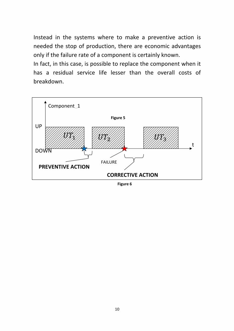
Instead in the systems where to make a preventive action is
needed the stop of production, there are economic advantages
only if the failure rate of a component is certainly known.
In fact, in this case, is possible to replace the component when it
has a residual service life lesser than the overall costs of
breakdown.
Figure 5
�� ���
FAILURE
CORRECTIVE ACTION
UP
DOWN
Component_1
t
PREVENTIVE ACTION
���
Figure 6

11
2.3 Condition Based Maintenance
The maintenance of the condition is the present and the future of maintenance because through knowledge of the technological process and goods to keep promoting the necessary response actions maintenance achieving the minimum overall cost. Incorporates inspections of the system in predetermined intervals to determine system condition. Depending on the outcome of an inspection, either a preventive or no maintenance activity is performed. Thus, CBM is a variety of a PM strategy with the difference, that the triggering event to perform a preventive maintenance activity is the expiring of a maintenance interval in the PM case, respectively the result of an inspection in CBM. Unlike in planned scheduled maintenance (PM), where maintenance is performed based upon predefined scheduled intervals, condition based maintenance is performed only when it is triggered by asset conditions. Compared with preventative maintenance, this increases the time between maintenance tasks, because maintenance is done on an as-needed basis. Apparently, CBM is only applicable when wear-out reserve is measurable. The goal of CBM is to spot upcoming equipment failure so maintenance can be proactively scheduled when it is needed - and not before. Asset conditions need to trigger maintenance within a long enough period before failure, so work can be finished before the asset fails or performance falls below the optimal level.

12
The guidelines for implementing a CBM system are explained in the following figure (7).
Condition Based Maintenance allows preventive and corrective actions to be scheduled at the optimal time thus reducing the total cost of ownership. Today, CBM methods are becoming more mature and improvement in technology are making it easier to gather, store and analyze data for CBM. In particular, CBM is highly effective where safety and reliability is the paramount concern such as the aircraft industry, semiconductor manufacturing, Nuclear, Oil and Gas.
SENSOR SIGNAL
DATA ACQUISITION
DATA PROCESSING
CONDITION MONITORING
PROGNOSIS OF RESIDUAL LIFETIME
DECISION SUPPORT
MAINTENANCE SCHEDULE
Figure 7

13
2.4 Data Input in Condition Based Maintenance
Acquisition of data is done by observing the state and condition of the production system with monitoring tool and devices. Among others, some of the monitoring tools are: • Vibration monitoring; • Lubrication monitoring; • Thermography; • Acoustic sound source localization; • Non-destructive thickness measuring with ultrasonic. In the following figure (8), it shown the diagram about the data input.
ANALYSIS DATA INPUT
DETERMINATION OF DEGRADATION
PREVENTIVE ACTION NO PREVENTIVE ACTION
Degradation (t)
t
Figure 8

14
2.5 Advantages Of Condition Based Maintenance
The advantages that the implementation of a CBM policy on
maintenance could bring are:
• CBM is performed while the asset is working, this lowers
disruptions to normal operations;
• Reduces the cost of asset failures;
• Improves equipment reliability; • Minimizes unscheduled downtime due to catastrophic failure • Minimizes time spent on maintenance; • Minimizes overtime costs by scheduling the activities • Minimizes requirement for emergency spare parts; •Optimized maintenance intervals (more optimal than manufacturer recommendations); •Improves worker safety; • Reduces the chances of collateral damage to the system.
But this advantages are compensated for the following disadvantages: • Condition monitoring test equipment is expensive to install, and databases cost money to analyze; • Cost to train staff – you need a knowledgeable professional to analyze the data and perform the work; • Fatigue or uniform wear failures are not easily detected with CBM measurements; • Condition sensors may not survive in the operating environment; • May require asset modifications to retrofit the system with sensors; • Unpredictable maintenance periods.

15
2.5 Vibration Monitoring
Rotating equipment such as compressors, pumps, motors all
exhibit a certain degree of vibration. As they degrade, or fall out
of alignment, the amount of vibration increases. Vibration
sensors can be used to detect when this becomes excessive.
The vibration monitoring can have different goals:
•to evaluate if a mechanical system respects the safety
standards;
•to shape the suspension of a machine, is needed take the
measurement of excitatory actions that arise when the machine
works .
• to find an adequate mathematical model of the mechanical
system vibrant, is needed before the measure of its response to
a known excitation.
The equipment to detect the vibrations comprises a transducer,
an amplifier and an indicator.

16
2.5 Trade-Off Maintenance Costs
The first step of this project has been to evaluate if is possible to
estimate a best level of the maintenance in a production system.
In fact, there is a trade-off between the costs of maintenance
and the costs of down time system. The sum between
maintenance costs (connected to the realization of maintenance)
and induced costs (which are related to the unavailability of
system) is the total cost of the maintenance function.
There will a minimum in this curve, and the goal is to find it.
Maintenance Costs
Down Time Costs
“Maintenance Level”
€
TOTAL
COSTS
Best Level
Figure 9

17
Chapter 3
A Condition Based Maintenance Model
Scientific research has shown a great interest for this type of
maintenance. In fact many studies propose different approaches
for apply a CBM.
A feature common to all models analysed, both in the case of
mathematical or simulative approaches and in case of discrete
or continues models, is the evaluation of thresholds
maintenance that identify the value of the wear parameter in
which should be done a certain action (inspection, preventive
maintenance, etc.).
It was studied a polity of Condition Based Maintenance because it turned out to be the most innovative. The CBM maintenance is becoming increasingly important because the development of advanced sensor and ICT technology makes the remote acquisition of condition monitoring data less costly, and condition data can improve diagnostics and prognostic of failures, which helps to reduce maintenance related costs further. Furthermore this maintenance strategy, in the scientific publications analyzed, turned out to be applied in the industries of advance capital goods (e.g., aviation, renewable energy and chemical process) due to the convenience of static intervals for the operations planning and coordination of maintenance resources (e.g., service engineers, maintenance equipments, spare parts).

18
3.1 Degradation Analysis
The most innovative aspect of this type of maintenance, is to
suppose that there is a link between degradation and failure of
component.
This is certainly true and it is confirmed from many studies that
showed how the bathtub curve is true only for a little
percentage of all components, but the problem is how can
evaluate the degradation of the component.
Assuming that is possible to determine at any given time a
parameter(e.g. temperature of engine, wearing of a brake,
vibrations of a FMS, etc.) that describes the wear of component,
is possible to have with this type of maintenance many
economical advantages.
As said before, the tools for evaluate these parameters are
expensive, so this type of maintenance is possible only in some
industrial business.
In a CBM maintenance the reliability of the system is studied in
function of a parameter linked with the time and other
characteristic aspects of the production system.
Assuming that is possible to determinate a deterioration
threshold, when the wear exceeds this threshold the component
enters in a period where is better to make a preventive
maintenance than wait the failure, because the residual safety
life of the component is lower than the overall costs of
breakdown.

19
The following figure (10) is shown a stochastic process of
degradation of a generic component prone to preventive
maintenance.
As in the figure (10 ) showed, the process of increasing of wear is a stochastic process. In fact: ∆ ��0, � � ≠ ∆ ��� , � �� if �0, � � = �� , � �� (1) The increase of wear in the same time intervals is different.
FAILURE LEVEL � Degradation (t)
t
PREVENTIVE ACTION
Figure 10

20
This is obvious because the increase of degradation depends mainly from two aspects: • work condition of machine; • work load of machine. Namely that degradation of a system depends from the condition where it works, there will be nominal conditions that the constructor identifies where the degradation process of the machine is known. But if the machine works in different condition, the degradation process is not can be determined. The same is for the production rate, if the machine works at the nominal rate has a degradation process known, but if it works with other rate, the degradation will be different. In this paper the approach used is to assess the failure of a device based on the characteristics of the process that caused its failure, normally a degradation process. Such an approach is common in assessing the amount of crack, the amount of erosion, and creep, and amount of contamination. Since many devices fail because of degradation, the degradation process is some type of stochastic process. For this reason the mathematical model that it was used to define the behaviour and the characteristics of the simulation model is a model that examines a stochastic degradation process.
21
3.2 Mathematical Model
The mathematical model that was studied is: “ A CBM policy for
stochastically deteriorating” of Grall, Berenguer and Dieulle, a
continuous and mathematical model that studies how is possible
to apply a CBM maintenance in a system consisting of N
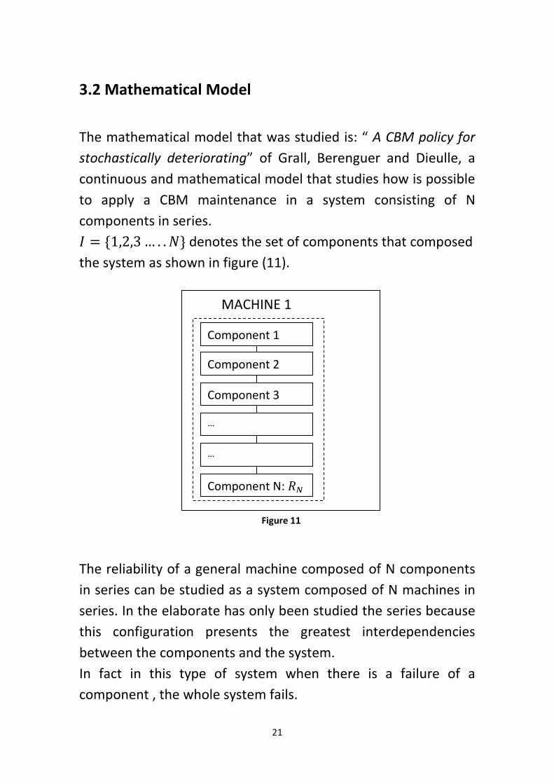
components in series. = {1,2,3 … . . '} denotes the set of components that composed
the system as shown in figure (11).
The reliability of a general machine composed of N components
in series can be studied as a system composed of N machines in
series. In the elaborate has only been studied the series because
this configuration presents the greatest interdependencies
between the components and the system.
In fact in this type of system when there is a failure of a
component , the whole system fails.
Component 1
MACHINE 1
Component 2
Component 3
…
…
Component N: ��
Figure 11

22
Through this initial research, it have been possible to
determinate which are the most important features that the
simulation model must have.
The mathematical formulation, given in appendix (2) , provides
the determination of minimum maintenance cost in function of
two variables:
• ): time interval between two inspections;
• � : threshold of wear for change the part.
is possible to determinate τ and Li that give me the minimum
cost in function of these two variables.
Figure 12
� Degradation(t)
t
τ 2τ …. nτ τ 2τ … nτ (n+1)τ
PREVENTIVE ACTION *+,-./.�012�2)� < �
NO PREVENTIVE ACTION FAILURE
1
2

23
So is possible to indentify two case:
1. When at the inspection in nτ the degradation is higher than
the threshold � , a PREVENTIVE ACTION will be taken in nτ. *+,-./.�012�2)� ≥ � → 6-+7+2�07+ 89�012
2. When at the inspection in nτ the degradation is lower than
the threshold � , but it increases fast in the interval
[nτ,(n+1)τ] and exceeds both the thresholds � and the
threshold of failure before the next inspection at the time:
(n+1)τ, a CORRECTIVE ACTION will be taken. *+,-./.�012�2)� < � → ': 6-+7+2�07+ 89�012
The figure (12) shows two aspects:
1. When is carried out a PM action, the component has a
residual service lifetime but it is substitute before the failure. In
this case it is lost money related to the residual service lifetime
of the component which is not used.
2. When is carried out a CM action, the component has not a
residual service lifetime, but there will be an overall cost of
breakdown.

24
In fact to determinate the threshold � , it must to solve a trade-
off between the residual service life of the component in money
and the overall cost of a breakdown, as the following figure(13)
shows.
The value of � is function of the overall cost of downtime. More
is high the overall cost downtime and lower is the value of � , and therefore the component is changed when it have yet high
residual service lifetime.
As explained in the previous pages, the most important
parameter that influences which type of maintenance have to
realise, is the overall cost of downtime.
For overall cost of downtime :
•high�PREVENTIVE MAINTENANCE;
•low �CORRECTIVE MAINTENANCE.
For Overall Costs Downtime is defined the total cost that we
have more if the production system have a stop.
Residual Service �
€
Best Li
Overall Costs Downtime
Figure 13

25
Chapter 4
SIMULATION IN MANAGEMENT DECISION MAKING
In today’s competitive business climate, careful planning and
analysis of alternative strategies and procedures are essential. In
an effort to derive maximum benefit from available resources ,
engineers and business planners have made mathematical and
computer modelling an important part of their planning
activities. Among these modelling techniques , simulation has
experienced a particularly dramatic increase in popularity
because of its broad range of applicability.
Simulation is simply the use of a computer model to “mimic” the
behaviour of a complicated system and thereby gain insight into
the performance of that system under a variety of
circumstances.
Simulations are often used to determinate how some aspect of a
system should be set up or operated.
The discrete-event simulation describes system that are assumed
to change instantaneously in response to certain sudden or
discrete events or occurrences.
When we choose to model a real-world system using discrete-
event simulation, we give up the ability to capture a degree of
detail that can only described as smooth continuous change. In
return, we get a simplicity that allows us to capture the
important features of many system that are too complex to
capture with continuous simulation.
26
Simulation Model
Create a model that reproduces the behavior of a complex
production system subject to maintenance on condition
represents a test, whose complexity is linked to the presence of
many variables associates and employees , such as for example:
• Wear parameters of the system components,
• Deterioration's laws of the components, and trend of this
parameters in time;
• Number and relationships of physical and logical connection
between the components,
• Relationship between the wear and failure,ect.
In this dissertation, the simulation approach was preferred at the
mathematical approach, because with a simulation software is
possible to realize a complex model that has a behaviour closer
to the reality.
The wear is identified as parameter of aging characterized by a
continuous and non-decreasing trend in the time. It was decided
to model the wear with different distributions, in order to
identify which was the one that reflects the real behavior. It is
supposed that a component can be considered fault if the wear
parameter exceeds a certain threshold. This hypothesis appears
to be significantly distant from experience, because the fault is
an event that can be linked to the wear of the component but
whose time of occurrence is a random variable. Therefore, the
probability of failure has been patterned by a distribution of
Weibull, not linked to the time, but to the parameter of wear, as
appears more correct from logical point of view.
27
4.1.1 Metamodel
In this model, it was studying a general system composed of N
components.
The main objective of the work was to build a model that was
valid to more industrial areas. For do this, it was studied a system
composed of N components in series. It was studying only the
series because it is the most important from the point of view of
reliability.
The difficulties found concern the fact that it is impossible to
perform a simulation with Arena and a consequent optimization
leaving not fixed, but variable, a number N of elements. For this,
we thought to build a modular model that represents only one
general system, but changing some variables is apply to many
production system.
In the model it was evaluated the production logic and the
maintenance logic together.
It was impossible to build only one model for simulate the both
logics because the entities in the production system model are
work pieces while in maintenance model are preventive or
corrective maintenance requests.

28
For this it was build a model formed by three sub-models, how
shown in the figure (14):
- one to simulate the maintenance system;
- one to simulate the production system;
- and one to link the two previous sub-models, that we called
sub-model of connection.
Figure 14
CONNECTION SUB-MODEL
MAINTENANCE SUB-MODEL
PRODUCTION SUB-MODEL

29
4.2 .1 The Logic Of The Model
As already mentioned, the model is split in three sub-models. For
each of them, the entities that flow in the logic are different.
In fact in the connection sub-model there is only a entity that
representing the machine, in the maintenance sub-model there
is only a entity that representing an inspection request, while in
the production sub-model there are more entities that
representing work pieces. In sub-models of connection and
maintenance there is only a entity that flow in a closed loop. This
choice has permitted to have a model more simply and less
“heavy" in the computational point of view.
In the following figure (15) , it was showed the model’s logic.
CONNECTION SUB-
MAINTENANCE PRODUCTION
MAINTENACE
REQUEST FOR
PREVENTIVE
MAINTENANCE
REQUEST FOR
CORRECTIVE
MAINTENANCE
WORKING
Figure 15

30
The production sub-model is in open loop, where with a rate of
arrival known, the entities flow from a Create module to a
Dispose module after have been passed the production logic.
When a failure occurred, this sub-model throws a signal to the
sub-model of connection that handles the request.
At the same way, the maintenance sub-model, that have a closed
loop logic, when after an inspection determines a degradation
level higher than threshold L_i, throws a signal to the sub-model
of connection.
The signal derived from the maintenance is a preventive action
request, while the signal derived from production is a corrective
action request. Both the requests generate a state change of the
entity, that from the working state passes to the maintenance
state.
When finishes the maintenance action , the entity returns to the
working state. So it flows in a closed loop, changing its state from
working to maintenance and from maintenance to working.

31
4.2.2 Connection Sub-Model
This sub-model have a “closed loop” logic, where only an entity
flows in the modules. This entity represent the machine or the
system object of study.
There are two possible state of this entity:
• Machine WORKING;
• Machine MAINTENANCE;
In the initial state, it supposed that the machine is working. This
choice simplifies the model and permits a study more realistic.
When after an inspection, the degradation level is higher than
the threshold � , the maintenance sub-model send a signal to
the connection sub-model, that handle the maintenance process.
When instead after the inspection, the degradation is less than � , the control logic does not make nothing and the machine
continues to work.
CONNECTION
SUB-MODEL
*+,-./.�012 > � REQUEST PREVENTVE ACTION
*+,-./.�012 < � NO ACTION
PREVENTIVE ACTION
Figure 16

32
In this way, after an inspection is possible to indentify two case:
•If *+,-./.�012 < � �No ACTION.
•If *+,-./.�012 ≥ � �PREVENTIVE ACTION.
The request of maintenance can arrive:
1. after an inspection;
2. when the degradation exceed the threshold of failure
before of an inspection;
3. when a random failure occurs.
When arrive a request of maintenance from the production sub-
model, it is a corrective maintenance action.
CONNECTION
SUB-MODEL
REQUEST FOR CORRECTIVE ACTION
RANDOM FAILURE
CORRECTIVE ACTION
*+,-./.�012 > <.0=>-+_*+,-./.�012
Figure 17

33
4.2.3 Maintenance Sub-Model
In this sub-model the entity symbolizes an inspection request,
and it is recycled for all time of simulation. In a real context it is
impossible, but in this way it was possible to overcome on the
limits of the student version of Arena(limit about the number of
entity).
Through Decide modules this entity produces inspection requests
in function of a scheduling read from an external file of Excel.
After an inspection if the wear exceeds the threshold � , a signal
has sent to the connection sub-model, which it provides to
replacement the part, while if the wear is lower of the threshold,
the entity flows into the closed loop and evaluates the next
inspection defined in the scheduling.
This sub-model reads the scheduling of inspections, performs the
inspection in function of the schedule, and carries out a request
of maintenance after an inspection when the wear of the
component has a value higher of the threshold of preventive
maintenance.
Therefore the goals of this sub-model are:
• count the time and evaluate when is the moment to achieve an
inspection, in function of the schedule,
• read the wear parameter and determine if is necessary a
preventive action or not;
• send a signal to the sub-model of connection if the wear is
higher of the preventive threshold;
• wait that preventive action is finished before to make a new
inspection of one other component.

34
4.2.4 Production Sub-Model
In the production sub-model the entities flow in a open-loop and
arrive with a ratio that is given from an external input.
This ratio is the production rate of the system.
The production is simulated with a module Process that takes up the machine for the production time. If the logic control,determines a value of degradation higher than the value of failure of the component, it throws a signal to the connection sub-model and the production is stopped. The same is made when arrives a random failure. When the machine is in maintenance, the work pieces enter in a module Hold that representing a queue. When the maintenance process is finished, a signal from the connection sub-model is threw to the production, that can restart to work. In this way it was been possible to shape the input buffer in function of: • production rate of the system; • time of maintenance of the system. As explained in the previous pages, the objective of the study it was been to build a model more general possible that was applicable in different business companies. In this mode we defined a general simulation model that with the change of the input variables it could be apply to make many considerations about the initial planning of the factory.

35
Description Data Input
In this chapter we were described the input data of the simulation model. All inputs data are read from an external file to give generality and modularity at model.
4.3.1 Failure Rate
To build a general model that was applicable to many different industrial areas,all inputs are read from an external file of Excel. In this way, it was possible to make a general model that with a change of the variables can be applied to solve many problem. It was assumed that in some way is possible to calculate the Rate Failure of each components. Is possible to have this data if the company have a management software like a CMMS: Computer Maintenance Management System, with it the company can have track of every failures of the system. In fact with a CMMS, the information about every failure of production system are tracked in the software. It was supposed that when the production system has a failure,is possible to input in CMMS the istant of failure,namely the parameter: • ttfi: time to failure component it

36
Then with many different algorithms, present in many scientific publications , can be determinate the parameter: λ(Rate Failure) for every components. The following figure(18) shows the scheme of application three different algorithms: 1. DM: Direct Method ; 2. IDM: Improved Direct Method ; 3. RM: Ranked Method . The explanation of these three methods is beyond the scope of this study. It have been study these alghoritms only to build a procedure to determinate a maintenance plan.
In the appendix (1) is shown an example of application of these three algorithms. The parameter λ is used like a input data to simulate the random failures of the system. In fact, from the probability theory7: @��< = A [hours]
If λ=constant
7 Statistical Theory of Reliability and Life Testing: Probability Models (1975)
ttfi[hours^-1]
153
320
432
619
ALGHORITM
DM-IDM-RM SIMULATION
MODEL λ
Figure 18

37
So if the component is in service life and it has a failure rate constant, the MTTF: Mean Time To Failure is defined in this mode. In this way, there will a logic in the production sub-model that will generate a failure every MTTF hours. In the following table(1) it is showed how is possible to calculate the parameter λ. In fact, if the company have a CMMS that tracks of the failures of each component, is possible to estimate λ.
@��< = 8B8 �8C�D � @D E-1/>9�012 FGF�+H<�DI�D'JK 1L L.0=>-+ 91HE12+2� M ℎ1>-G+.-L.0=>-+G+.- O = P ℎ1>-L.0=>-+Q
R = 1@@�< Sℎ1>-TU
CODEX
COMPONENT
sum
duration
stops
[min]
sum
duration
stops
[hours]
frequency
of the
stops
MDT:
mean
down
time
[min]
MTTF[hours] λ[h^-1]=1/MTBF
M1-01 159 2.65 11 14.45 727.27 0.0014
M1-02 234 3.9 9 26.00 888.89 0.0011
M1-03 74 1.23 6 12.33 1333.33 0.0008
M1-04 103 1.72 3 34.33 2666.67 0.0004
M1-05 127 2.12 6 21.17 1333.33 0.0008
M1-06 245 4.08 11 22.27 727.27 0.0014
M1-07 121 2.02 15 8.07 533.33 0.0019
M1-08 21 0.35 7 3.00 1142.86 0.0009
M1-09 36 0.60 5 7.20 1600.00 0.0006
M1-10 45 0.75 9 5.00 888.89 0.0011
M1-11 78 1.30 13 6.00 615.38 0.0016
M1-12 95 1.58 11 8.64 727.27 0.0014
M1-13 36 0.60 1 36.00 8000.00 0.0001
M1-14 258 4.30 24 10.75 333.33 0.0030
M1-15 301 5.02 23 13.09 347.83 0.0029
Table 1

38
4.3.2 Frequency Of Inspection
Same as the failure rate λ, the frequency of inspection and the date of first inspection are read from an external file of Excel. The maintenance sub-model reads the date of the first inspection and when the simulation's watch arrive to this date, it makes an inspection. At the same way , for every time interval equal to the frequency of the inspection, repeats the inspection for the component.
CODEX
COMPONENTS
Date FIRST
ispection
Day of year of FIRST
ispection
Frequency
inspection [days]
Tisp [min]
1 07/01/2015 7 7 10
2 08/01/2015 7 7 10
3 09/01/2015 7 7 10
4 10/01/2015 7 7 10
5 11/01/2015 7 7 10
6 12/01/2015 7 7 10
7 13/01/2015 7 7 10
8 14/01/2015 7 7 10
9 15/01/2015 7 7 10
10 16/01/2015 7 7 10
11 17/01/2015 7 7 10
12 18/01/2015 7 7 10
13 19/01/2015 7 7 10
14 20/01/2015 7 7 10
15 21/01/2015 7 7 10
Table 2
So in the maintenance sub-model , the entity flows in a closed-loop, and it becomes a request of inspection when arrive the date of inspection for the component. When for one day , there are not inspections to make, the entity flows in a loop and go to the next day.

39
4.3.3 Degradation Parameter
To evaluate the degradation of the component, the model reads from an external file, shown in table (3) , the following parameters: • Initial wear �the initial degradation of the component. • L preventive � the threshold of preventive action. • L failure �the threshold of corrective action. The initial wear is supposed equal to zero, therefore the component is new , when start the simulation. λ costant L preventive
(% wear)
L
failure
(% wear)
Initial
Wear
Num hours
for exceed
Lp
Num days for
exceed Lf
ρ=Lp/Lf
0.0013 0.9 1 0 692.307 32.05128205 0.9
0.0013 0.9 1 0 692.308 32.05128205 0.9
0.0013 0.9 1 0 692.308 32.05128205 0.9
0.0013 0.9 1 0 692.308 32.05128205 0.9
0.0013 0.9 1 0 692.308 32.05128205 0.9
0.0013 0.9 1 0 692.308 32.05128205 0.9
0.0013 0.9 1 0 692.308 32.05128205 0.9
0.0013 0.9 1 0 692.308 32.05128205 0.9
0.0013 0.9 1 0 692.308 32.05128205 0.9
0.0013 0.9 1 0 692.308 32.05128205 0.9
0.0013 0.9 1 0 692.308 32.05128205 0.9
0.0013 0.9 1 0 692.308 32.05128205 0.9
0.0013 0.9 1 0 692.308 32.05128205 0.9
0.0013 0.9 1 0 692.308 32.05128205 0.9
0.0013 0.9 1 0 692.308 32.05128205 0.9
Table 3
In the file there is the parameter ρ that is defined as: V = � E-+7+2�07+� 91--+9�07+
It is reported because in the optimization of the model, it was studied how changes the total cost in function of this parameter.

40
4.3.4 Service Level
Service level measures the performance of a system. Certain goals are defined and the service level gives the percentage to which those goals should be achieved. In this case the service level determinate how many times there is the spare part in the warehouse after a failure. So it can be defined for each component in the following mode: •Service Level: probability to find the spare part in the warehouse, after the breakdown of the component.
CODEX COMPONENT SERVICE LEVEL [%] SUPPLY TIME [min]
1 90.0000 100.00000
2 90.0000 100.00000
3 90.0000 100.00000
4 90.0000 100.00000
5 90.0000 100.00000
6 90.0000 100.00000
7 90.0000 100.00000
8 90.0000 100.00000
9 90.0000 100.00000
10 90.0000 100.00000
11 90.0000 100.00000
12 90.0000 100.00000
13 90.0000 100.00000
14 90.0000 100.00000
15 90.0000 100.00000
Table 4
In the table(4) it shown the data input related to the Service Level and the Supply Time. In fact in the simulation model when a component fails, with a percentage equal to the SL, the spare part is in the warehouse, and with a percentage equal to (1-SL) it is not in the warehouse and a supply time is needed. The table(4) is only an example, in fact is impossible that all components have the same SL and supply time.
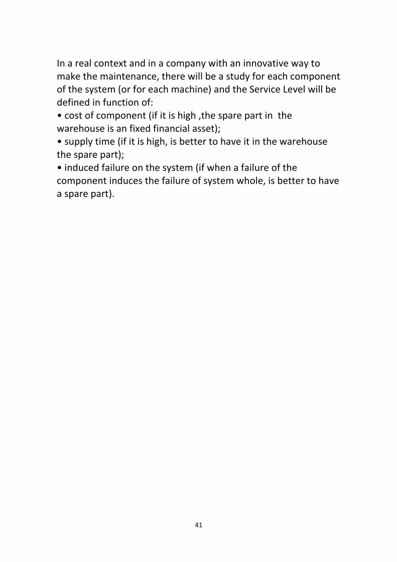
41
In a real context and in a company with an innovative way to make the maintenance, there will be a study for each component of the system (or for each machine) and the Service Level will be defined in function of: • cost of component (if it is high ,the spare part in the warehouse is an fixed financial asset); • supply time (if it is high, is better to have it in the warehouse the spare part); • induced failure on the system (if when a failure of the component induces the failure of system whole, is better to have a spare part).

42
4.3.5 Data Input Diagram
As already definite in the previous paragraphs, the input data of the model are: • λ : Failure rate; • day of the first inspection; • frequency of inspections; • initial degradation; • L preventive; • L failure. • Service Level. In the simulation model it was evaluated how changes the output in function of the input. Especially the objective of the dissertation it has been to check on which variables have more impact in the choice of the maintenance strategies. In fact without a real application, the goal of the research was to determinate which characteristics are important for apply a CBM policy. With repeated analysis in Arena, it was been possible to investigate how changes the total cost of maintenance in function of the inputs previously described.

43
4.3.6 The Creation Of The Entities
The creation of the entities is an input that is possible to insert from an external command in Arena. It has been assumption that the first entity that enters in the system is the machine, that flows through more module ReadWrite in the connection sub-model and determines the features of the system.
It is create only one entity when the simulation start. The entity is called M1. The parameter First Creation is set to 0.0 and Max Arrivals is set to 1, so when start the simulation, the model create the entity machine that flows in a closed loop for all time of analysis.

44
In the same way, we have in the maintenance sub-model only one entity that flows in a closed loop. While in the production sub-model, we have more entity that flow in logic. In fact in this sub-model, the entities are a work pieces.
In production sub-model, the entities are created in fixed intervals of time equal to 1 hour and the parameter Max Arrivals is set to Infinite, so a entity is created each hour for all simulation time. The reason to insert an inter-arrival time between two consecutive entities will be more clear when we will describe the degradation increase process. In fact, with the goal to investigate only the maintenance of the production system, we have supposed that the degradation of the component increases every hour of work of the machine. In this way we can examine the degradation process of the component and we can pass the limits of student version of Arena.

45
4.4.1 Simulation Model Description
To have a more easy definition of the simulation model built with the Arena software,we divided it in more sections, each one with a different logic. Is possible to define 6 different sections, that we describe in the following mode: 1. Reading external file; 2. System control; 3. Daily watch; 4. Phase of inspection; 5. Production logic; 6. Degradation process. In the following pages it was illustrated each section for have a more complete description of the simulation model. Each section have a own logic, but it is linked with the others through Boolean variables that change own value when an entity flows in the Assign modules.

46
4.4.2 Reading External Files
When the entity “machine” is created, it flows through more module ReadWrite in the connection sub-model and determines the features of the system.
The entity reads for each components of the system, the following parameters: • λ: failure rate of the component [hour^-1]; •Initial degradation; • Service Level of the component [%]; • Supply time [hours] • α and β of the Weibull Distribution of the degradation process; • L preventive and L corrective [%]; • Date of first inspection; • Frequency of inspections [days], • Duration of inspection [hours]; • Duration of maintenance action [hours].

47
When the entity flows in the ReadWrite module, reads the parameters and writes them in an array that is used in the model. How showed in the following figure, Arena reads the parameter λ from an external file and writes it in one array with 16 lines ( the number of the components) and one column( the number of parameters).
The software read sixteen values for each variables, but it work with only fifteen because there are problems with the last value of the array. In the input we put fifteen values, but it is possible to introduce more values in function of the number of components of the system. This is possible only with a change of variable because, how explain previously, the goal of the research has been to build a general model that is possible to apply in different context.

48
Therefore we can definite the entity machine like a bin that contain every features of the production system.
In this way if a system has different features or if certain values are not available, the model remain valid. Is needed to change the path of the entity, and add or remove the ReadWrite modules in function of the data inputs available.
FILE EXCEL
MODULE
READWRITE
MACHINE
ENTITY
λ β α SL
SupplyTime
Frequency
λ β α SL
SupplyTime
Frequency

49
4.4.3 Control System
This section of the model is the most important because it handles the connection logic between the production and the maintenance. When the entity Machine exits from the last ReadWrite, it flows in a Hold module. When the entity is in this module it means that the machine is working, while if it exits of this module it means that the machine is failure. This module Hold is set of Wait a Signal, so it waits a signal from the production( if there is a failure) or from the maintenance (if after an inspection is need to make a preventive action).
When the entity Machine exits from the module called System
Working, it means that there is a preventive or corrective maintenance request. At this point the entity flows through more Assign module that are needed for determine the final statistics.

50
In this logic we have a Decide module that reads the probability to find in the warehouse the spare part, after a failure. If with probability equal to Service Level the spare part is in the warehouse, the system handles the maintenance action, while if the spare part there is not in the warehouse ,with probability equal to (1-SL) the system waits to finish the supply process before, and then it handles the maintenance action.
In this way it has been possible to evaluate how changes the
breakdown time of the system in function of the Service Level of
each component. As said previously, the Service Level for each
component is a value that is possible to determinate only after a
specific study on your features.

51
The maintenance action is simulated with a Process module that
seize a Maintenair resource for a time equal to Tmain. This last
parameter is different for each component, and representing the
time to change the component. It is read from an external file
and is characteristic for each component.
We have inserted a standard deviation to simulate that the
replacement time is not a fixed time but it can change in an
interval.
So when the entity exits from this module it means that the
maintenance action is finished, so the Machine flows in more
Assign modules, writes the data about the failure, and then
returns in the Hold module that simulates machine working.

52
In the following figure, it is showed the complete logic of the
system control.
There are many Assign modules that are needed to write the
final report.
In these modules more variables change the own value when the
entity pass.

53
4.4.4 Daily Watch
This section of the model handles the inspections on the
production system. The date of first inspection and the
frequency, are read for each component from an external file, as
before we are explained.
There is only an entity that flows in a closed loop. It passes
across more Decide module, and it evaluates if it is the day of the
control for each components.
The simulation's watch calculates the time, in fact there are in
Arena more variables that determinate the minute, the hour,
and the day of simulation's time.
We used these variables to determinate when is the day of one
inspection.
So for each day, this logic checks if there is inspection to make
with a Decide module.

54
When arrive the day of the inspection on the component i, the
logic simulates the control of the system with a Process module,
as Inspection Action. It is a process that seize a inspector
resource for a time equal to the time needed to make that
action. This time is read from an external file.
We use two different resource for the inspections and for the
maintenance actions because in final we want to do
considerations about the costs and about the workers needed to
the production system. If instead it is not the day of the control
of the component i, the logic evaluates the next component.
When the dates of every component are checked and every
action of the day are processed, the logic pass to the next day
and repeat the control.

55
Besides when a inspection is finished, the system assign the next
date of the inspection with a Assign module.
Every data input are read from an external file because we want to built a general model, that is possible to apply in more business only with the change of the variables. How shows the figure the new value of the variable (type Others) is equal to first_control+frequency. In this way when an inspection is finished this variables is updated at the next control day. For each variable is specified the index i, that defines which component is.

56
4.4.5 Phase Of Inspection
When the simulation's watch determines the day of the inspection of component i, the system makes this inspection. We already have explain that an inspection is simulated with a process that seize a resource. After an inspection if the instantaneous degradation of the component exceed the preventive threshold, a signal is throw to the connection sub-model that handles the request.
With a Decide module the logic evaluates if the instantaneous degradation of the component exceed the threshold.

57
Then we have a Assign module that changes the variables needed to write the final report and a Signal module that throws a signal to the connection sub-model. This signal arrive to the connection sub-model, it handles this request while the maintenance sub-model waits for the time need to finish the preventive action.

58
4.4.6 Production Logic
This section of the model simulates the production system. In this sub-model,the entities flow in a open loop and simulate the work pieces.
There is a queue that simulates the input queue of the production system. Here the work pieces wait if the machine is not available. Then we have a Separate module that duplicates the work pieces.

59
We use this module to duplicate the processes. There will be the original work piece that flows in the production process and a other duplicate that flows in other section to increase the degradation of the machine. In this way it was simulated the production system and the degradation process, so that the wear of the machine increase only if the system works. We have been supposed that the degradation increases every hour of work, so the production time is set to one hour. This choice permitted to simulated a more realist degradation process. The production is simulated with a Process module that seize the machine resource.

60
4.4.7 Degradation Process
The degradation process is simulated with a dummy entity that flows in a Process module to increase the wear of the component.

61
There is a Hold module called ScrollM1 where the dummy entity waits the finish of the production time. When it is passed the production time, the degradation of each component is increased with an Assign module.
For each component it was defined a variable called instantaneous_wear. This variable is increased every hour for a value equal to parameter lambda, previously defined. Then we have a Decide module that evaluates the instantaneous wear of each component. This Decide handles the random failure of the system also. In fact it throws a signal to the connection sub-model if occurred two event: •when the instantaneous degradation of the component exceed the threshold of corrective action; •and when the a random failure occurs.

62
In this Decide we use the following expression: �1, P�1, 1�' <�0,1�Q < {SW�ℎ, 1� ∗ �1,�02F�.2�.2+1>FYZ[\�ℎ, 1�U − W�ℎ, 1� ∗ logS.�ℎ, 1�U}
With this expression it is simulated the probability that a random failure occurs. It is supposed that the random failure of each component follows a Weibull distribution. In fact, if we want to study the probability that a component has a random failure before of a known time, we have to study the cumulative function of the distribution.

63
The cumulative function of the Weibull distribution8 is: <��� = 1 − +T�ab�c: probability that the component has a failure
before the time t. With this expression, Arena had a problem to calculate an exponential function, so we solved the same expression with the logarithms. 1 − <��� = +�ab�c
� logS1 − <���U = log S+T�ab�cU � logS1 − <���U = −�de�f�
− logS1 − <���U = �de�f� logS1 − <���UT = �de�f� log g Th�d�i = �de�f
�
log Slog P 11 − <���Q = j log � − j log k
In the expression inserted in Arena we have: • b(h,1): parameter β of the component i; • alpha(h,1):parameter α of the component i; • UNIF(0,1): random parameter ∈ S0,1U; • instantaneous_wear: parameter t for simulate the time.
This is the expression for simulate the random failure. Instead to simulate the failure when the degradation exceed the threshold of corrective action we use the following formula: 02F�.2�.2+1>FYZ[\�m,� > �no\\Znd pZ�m,�
8 Weibull, W. (1951)

64
This sub-model does these two controls every hour of production and for each component. When one of these expressions is true a signal is throws to the connection sub-model. As for the maintenance sub-model, also in this there is an Assign module for change of the variables needed to write the final report and a Hold module for wait the finish of the maintenance action.

65
5.1 Final Report
The final report shows how the key performance indices of the production system in function of the input variables change. Through more Assign and Write modules we determinate the diary of failures. The format of the failure diary is showed in the following table(3) and it change for every simulation.
CODEX
COMPONENTS
ISTANT
FAILURE
TYPE ACTION
[1:Preventive;2:Corrective]
BREAKDOWN
TIME 12 49620 2 10.31449526
11 49670 1 9.887851741
14 49709.88785 1 9.478516378
3 55630.3145 2 10.16732162
6 80329.36637 1 10.50765707
7 80349.87403 1 10.33308891
12 99260.48182 2 9.95961022
14 99510.44143 2 10.35298101
9 100840.2071 1 9.428141099
11 100869.6353 1 10.0209164
3 111029.6562 1 10.1664712
13 111139.8226 1 9.78436937
10 121349.607 1 9.839624196
2 131509.4466 1 8.671332813
12 148918.118 2 9.692903761
14 149347.8109 2 9.646422067
11 152068.118 1 9.368372042
3 162227.4863 1 109.400235
6 162366.8866 1 10.10916755
7 162386.9957 1 9.422776016
12 198636.8866 2 10.34947275
14 199247.236 2 8.864165881
9 203336.4185 1 109.8714488
11 203466.29 1 10.15130041
3 213626.4413 1 9.168704408
8 223915.61 1 9.938691805
13 223975.5487 1 10.70310963
6 244376.2518 1 109.8010498
7 244496.0528 1 9.492363444
Table 5
66
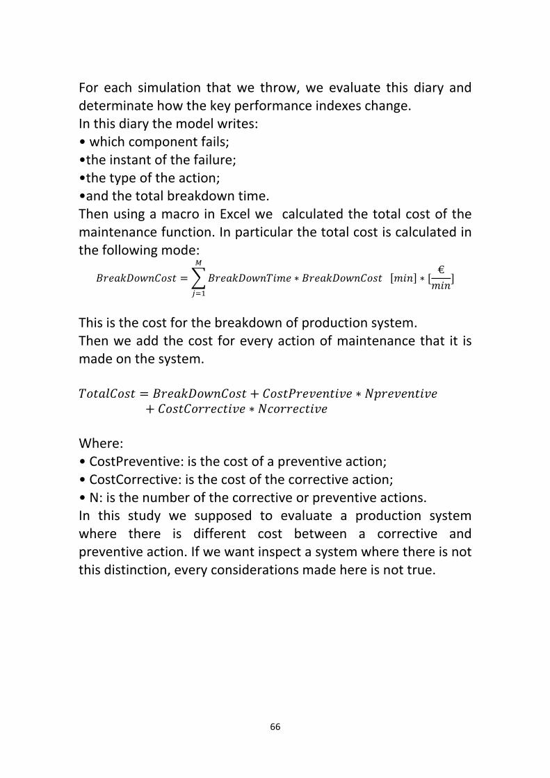
For each simulation that we throw, we evaluate this diary and determinate how the key performance indexes change. In this diary the model writes: • which component fails; •the instant of the failure; •the type of the action; •and the total breakdown time. Then using a macro in Excel we calculated the total cost of the maintenance function. In particular the total cost is calculated in the following mode:
C-+.q*1r2J1F� = s C-+.q*1r2�0H+ ∗ C-+.q*1r2J1F� SH02U ∗ S €H02U�u�
This is the cost for the breakdown of production system. Then we add the cost for every action of maintenance that it is made on the system. �1�.=J1F� = C-+.q*1r2J1F� + J1F�6-+7+2�07+ ∗ 'E-+7+2�07++ J1F�J1--+9�07+ ∗ '91--+9�07+
Where: • CostPreventive: is the cost of a preventive action; • CostCorrective: is the cost of the corrective action; • N: is the number of the corrective or preventive actions. In this study we supposed to evaluate a production system where there is different cost between a corrective and preventive action. If we want inspect a system where there is not this distinction, every considerations made here is not true.

67
5.2 Output Of Arena
The final considerations have been done in function of the diary of failure and of the statistics that have been defined in Arena. In particular for each simulation, Arena calculates the following parameter: •Total Breakdown time of the production system; •Total actions of maintenance; •Total inspections; •Number of preventive action; •Number of corrective action; •Total cost of the maintenance function. An example of the output of Arena, is showed in the following figure(20).
Figure 19
This output is related to a simulation of one year with a low threshold of preventive action. In fact in this case, we have only one corrective action, while all other actions are preventive. This is only an example, during the research we made many different analysis changing every time the input data. The output of each simulation it was put in an Excel file, and it has been the input for the following considerations about the advantages of a CBM policy.
68
Final Considerations
With this model we have been determined some general considerations about the economic convenience of a CBM polity. In particular we evaluated the change of the costs in function of the input variables.
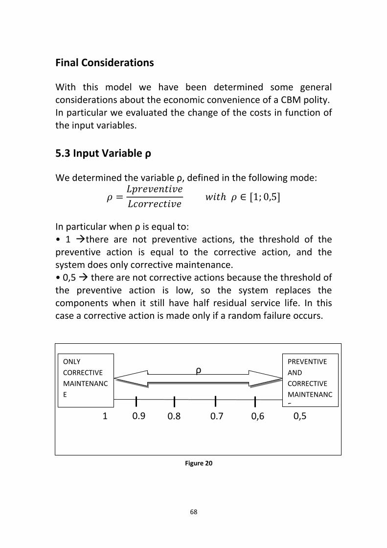
5.3 Input Variable ρ
We determined the variable ρ, defined in the following mode: V = �E-+7+2�07+�91--+9�07+ r0�ℎ V ∈ S1; 0,5U
In particular when ρ is equal to: • 1 �there are not preventive actions, the threshold of the preventive action is equal to the corrective action, and the system does only corrective maintenance. • 0,5 � there are not corrective actions because the threshold of the preventive action is low, so the system replaces the components when it still have half residual service life. In this case a corrective action is made only if a random failure occurs.
ρ
1 0.9 0.8 0.7 0,5 0,6
ONLY
CORRECTIVE
MAINTENANC
E
PREVENTIVE
AND
CORRECTIVE
MAINTENANC
E
Figure 20

We have studied the changing the variable.
The figure (22) shows how the of ρ. As was to expect the corrective actions increase when there is a decrease of parameter ρ , because the maintenance function replaces the component when it have service residual life still.While the preventive actioit means that the components are replaced when have little service residual life .
69
ave studied the changing the total actions in function of this
Figure 21
) shows how the actions types change in function
As was to expect the corrective actions increase when there is a decrease of parameter ρ , because the maintenance function replaces the component when it have service residual life still.While the preventive actions decrease when ρ increases because it means that the components are replaced when have little service residual life .
total actions in function of this
actions types change in function
As was to expect the corrective actions increase when there is a decrease of parameter ρ , because the maintenance function replaces the component when it have service residual life still.
ns decrease when ρ increases because it means that the components are replaced when have little

5.4 Input Variable ω With Weekly Inspection
We determinate the variable ω, defined in the following mode:y = JJ
It is the relation between the cost of a preventive action and of a corrective action. Higher is the value of this variable and higher is the overall cost of a breakdown of the productiothat the cost of a corrective action is possible to be cost of the preventive action. In function of this variable and of ρ,we studied the changing of the total cost of the maintenance if we have weekly inspectionson the components.
70
Input Variable ω With Weekly Inspection
We determinate the variable ω, defined in the following mode:J 91--+9�07+ E-+7+2�07+ r0�ℎ y ∈ S1; 4U
It is the relation between the cost of a preventive action and of a
Higher is the value of this variable and higher is the overall cost of a breakdown of the production system. We have that the cost of a corrective action is possible to be four time the cost of the preventive action.
In function of this variable and of ρ,we studied the changing of the total cost of the maintenance if we have weekly inspectionson the components.
Figure 22
We determinate the variable ω, defined in the following mode:
It is the relation between the cost of a preventive action and of a
Higher is the value of this variable and higher is the overall cost have supposed
four time the
In function of this variable and of ρ,we studied the changing of the total cost of the maintenance if we have weekly inspections

71
In the figure is possible to evaluate that: • when ρ=1, namely when there is only corrective maintenance in the system, the increase of total cost is proportional at the variable ω increase. It was predicted because if we have only corrective maintenance, when increase the cost of a corrective action increases also the total cost. • when ρ=0,9, we have corrective and preventive maintenance. In this case the total cost for every value of ω is lower than the total cost that we have in case of only corrective maintenance. The total cost with ρ=0,9 is higher than the cost of the corrective maintenance only if ω=1,namely if there is not an overall cost of the breakdown. • when ρ=0,8 or values lower, we have only preventive maintenance, so the total cost does not change in function of ω. For values of ρ lower than 0,8,there is only preventive maintenance, and the total cost fluctuates in function of the number of the preventive action. In fact lower is ρ and more preventive action on the system are needed. The most important considerations that is possible to determine with this graphic is that with ρ=0,9, the total cost is lower than all others case. So if is possible to evaluate the degradation of the component and replace it when it has service residual life low, this type of maintenance policy can give economic advantages.

5.5 Input Variable ω With Monthly Inspection
Besides we studied the change of total costs when there are monthly inspections in the production system.
In this case we have only preventive maintenance, if the system replaces the components when it still have half residual service life, namely when ρ=0,5.So with monthly inspections preventive maintenance is lower respect to previous case.
72
Input Variable ω With Monthly Inspection
Besides we studied the change of total costs when there are ctions in the production system.
Figure 23
In this case we have only preventive maintenance, if the system replaces the components when it still have half residual service life, namely when ρ=0,5. So with monthly inspections the threshold when there is only preventive maintenance is lower respect to previous case.
Besides we studied the change of total costs when there are
In this case we have only preventive maintenance, if the system replaces the components when it still have half residual service
the threshold when there is only preventive maintenance is lower respect to previous case.

The trend of the total cost in function of ω and ρ is showed in the following figure (25).
In this case the total means that is possible to determine the best maintenance policy because there is a minimum.Also in this instance the minimum for each trend in function of ω there is when ρ=0,9, this means that for each value oinputs, is possible to determinate the best strategies of maintenance only when there is a parameter linked to the degradation that is possible to evaluatIf is impossible to determinate this parameter is better to make only corrective maintendegradation of the component is expensive.
73
The trend of the total cost in function of ω and ρ is showed in the ).
Figure 24
In this case the total cost in function of ω is higher variable, it means that is possible to determine the best maintenance policy because there is a minimum. Also in this instance the minimum for each trend in function of ω there is when ρ=0,9, this means that for each value oinputs, is possible to determinate the best strategies of maintenance only when there is a parameter linked to the degradation that is possible to evaluate. If is impossible to determinate this parameter is better to make only corrective maintenance because the equipment to study the degradation of the component is expensive.
The trend of the total cost in function of ω and ρ is showed in the
cost in function of ω is higher variable, it means that is possible to determine the best maintenance policy
Also in this instance the minimum for each trend in function of ω there is when ρ=0,9, this means that for each value of the data inputs, is possible to determinate the best strategies of maintenance only when there is a parameter linked to the
If is impossible to determinate this parameter is better to make ance because the equipment to study the

74
5.7 Matrices To Find The Best Policy Of Maintenance
In particular the trend of the costs when the inspections are monthly, is always decreasing, so in this case is possible to have more economic advantages. These are general considerations in function of the initial hypothesis,these outputs can be different if the input changing. But the goal of the elaborate was to determine general matrices where in function of more variables is possible to identify the best maintenance policy for the company. In particular is possible to make an ABC analysis and make a
cluster of components in function of the following variables:
• ratio between the costs of a preventive action and a corrective
action: k = �{|}~}a�~}���||}�a�~}
• probability of failure induced;
• costs induced of downtime;
• knowledge of degradation trend.
These information are in the data base of the company if a
management software ,like a CMMS, is used from the
maintenance function. In fact with this equipment is possible to
have track about the failure of each component. In factories
highly evolved, is possible to insert in a CMMS software many
information, for example ttf (TimeToFailure of the component),
instant of last failure, cost of replaces, breakdown cost of the
production system, supply time, etc.

75
In the following figure(26), we clustered the components in
function of the first two parameters α and probability of induced
failure. This analysis shows that:
•the PREVENTIVE MAINTENANCE is cost-competitive if the
parameter α is low and the probability of induced failure is high.
In fact:
�if α∈(0,1]; (because the maximum cost of preventive action
can’t be higher than the cost of corrective action ) is low means
that the Cprev<<Ccorr, so is better to make a preventive action
than a corrective action because there is an economic
advantage.
�if the probability of induced failure is high means that a failure
can induce other failures,by increasing the downtime cost.
•the CORRECTIVE MAINTENANCE, instead , is cost-competitive if
α is high and the probability of induced failure is low. In fact:
�if α∈(0,1]; is high means that the Cprev≈Ccorr, so there aren’t
many difference between the costs of a corrective action and an
a preventive action.
Is better wait the failure and after change the part.
�if the probability of induced failure is low means that a failure
doesn’t induce others failures in the system.

76
Figure 25
ω=Cprev/Ccorr
Probability failure induced
PREVENTIVE
MAINTENANCE
CORRECTIVE
MAINTENANCE

77
Instead in the following figure(27), we clustered the components
in function of the others two parameters, the costs induced of
downtime and the level of knowledge of degradation trend.
Figure 26
Level of
knowledge
Degradation
trend
Costs induced
PREVENTIVE
MAINTENANCE
CORRECTIVE
MAINTENANCE

78
In this case, we are showing that:
•the preventive maintenance is competitive cost if is known the
degradation trend in the time and the induced costs of
downtime are high. This because:
�if is known the degradation's trend means that is possible
change the part when it arrive to have a degradation near to the
failure, so we know more or less when the components can fail
and we make a preventive action before.
�if the induced costs of downtime are high means that when a
component has a failure there is a high induced cost on the
machine, so is better change the part before that it has a failure.
•the corrective maintenance is more competitive than the
preventive maintenance when the knowledge of degradation's
trend is low and the induced costs are low, because:
�if the degradation's trend is not known,means that the
components have a high lumpyness, so it have a useful life very
variable and it’s impossible to estimate when is convenient
change the part.
�if the induced costs are low means that when a component
has a failure isn’t a problem because the machine do not have a
failure, so is better to wait the failure.

79
In the following figure (28) it is showed the matrix to indentify
the best maintenance polity in function of all variables previously
considered.
Figure 27
ρ
ω
CORRECTIVE
MAINTENANCE
Probability
induced failure/
Induced cost
HIGH
PREVENTIVE
MAINTENANCE
LOW

80
5.9 CMMS Software
A CMMS software package maintains a computer database of
information about an organization’s maintenance operations.
This information is intended to help maintenance workers do
their jobs more effectively (for example, determining which
machines require maintenance and which storerooms contain
the spare parts they need) and to help management make
informed decisions (for example, calculating the cost of machine
breakdown repair versus preventive maintenance for each
machine, possibly leading to better allocation of resources).
CMMS data may also be used to verify regulatory compliance.
During the research the software CMMS that it has been possible
to analyse has an application of input as that of the following
figure ( ):
Figure 28
Where is possible to indentify many information:
• work orders;
• equipment codex;
• work order description;
• worker assignment;
• schelule of work;
• type of action.

81
If is possible to have this type of information about the
maintenance of the production system then is possible to define
many considerations about the best strategies of maintenance.
moreover the data input of the simulation model are defined in
the same way, so if is available a CMMS software, the simulation
model can be used for determinate the total cost of the function.

82
Determinate a Maintenance Plan
If the company uses a CMMS software for organize the maintenance function, and evaluates what are the best strategies of maintenance with the use of mathematical or simulation equipment, is possible to define the maintenance plan . The key steps in preparing a typical maintenance plan are: • (1) Prepare an asset inventory - identifying the physical features (e.g., area, material,etc.) of all assets (e.g., schools, roads, etc.) which require maintenance; •(2) Identify maintenance activity and tasks - defining the type of maintenance task (activity) to be performed on each asset and what work should be done under each activity, e.g. • (3) Identify the frequency of the task - determining how often the activities should be performed (frequency of service); this is important particularly in preventive type of maintenance. Emergency or reactive type of repairs are unpredictable, but with good preventive maintenance, the frequency of emergency situations occurring may be reduced; • (4) Estimate the time required to complete the task - indicating how long each task should take to complete; • (5) Develop an annual work schedule - planning what time the maintenance work for the entire year should take place; • (6) Prepare and issue a work order - identifying what, when, where and by whom maintenance work is to be done; • (7) Determine a Budget- determining the costs for all maintenance activities by calculating labour hours, material, equipment, and contracting costs. For the first three steps a CMMS software is needed, while for the last step, namely determine a budget, a simulation model with Arena can be the best equipment to use.

83
APPENDIX 1
Application example of calculation Hazard Failure
This appendix shows the application of three algorithms used for the definition of the parameter λ (Hazard Failure Rate). We used three different algorithms because we want to determinate the difference between the values of λ that the three methods give back.
CALCULATION BEST λ EXP
INPUT
DM: direct method n= 4
i ttfi[hours]
F(ti)= i/n R(ti)=1- F(ti)
f(ti)=1/[n*(ti+1-ti)] λ(ti)=1/[(n-i)*(ti+1-ti)]
1 153 0.25 0.75 0.0015 0.0020
2 320 0.5 0.5 0.0022 0.0045
3 432 0.75 0.25 0.0013 0.0053
4 619 1 0 0.0000 0.0000
λ= 0.001243113
IDM:improved direct method n= 4
i ttfi[hours]
F(ti)= i/(n+1) R(ti)=1- F(ti)
f(ti)=1/[(n+1)*(ti+1-ti)]
λ(ti)=1/[(n+1-i)*(ti+1-ti)]
1 153 0.2 0.8 0.0012 0.0015
2 320 0.4 0.6 0.0018 0.0030
3 432 0.6 0.4 0.0011 0.0027
4 619 0.8 0.2 0.0000 0.0000
λ= 0.003025143
RM:rank method n= 4
i ttfi[hours]
F(ti)= (i-0,3)/(n+1)
R(ti)=1- F(ti)
f(ti)=1/[(n+0,4)*(ti+1-ti)]
λ(ti)=1/[(n+0,7-i)*(ti+1-ti)]
1 153 0.16 0.84 0.0014 0.0016
2 320 0.39 0.61 0.0020 0.0033
3 432 0.61 0.39 0.0012 0.0031
4 619 0.84 0.16 0.0000 0.0000
λ= 0.003625186

84
In this case we supposed to have track only of the last four ttf. This because we do not have a real application, but we want to evaluate the difference between these three method. We used to calculate λ: • Direct Method; • Improved Direct Method; • Rank Method. Then we used these three method to calculate the parameters α and β if the trend of failures of component follows a Weibull distribution.
CALCULATION BEST β and α WEIBULL
INPUT
DM: direct method n= 4
i ttfi[hours]
F(ti)= i/n R(ti)=1- F(ti)
f(ti)=1/[n*(ti+1-ti)] λ(ti)=1/[(n-i)*(ti+1-ti)]
1 153 0.25 0.75 0.0015 0.0020
2 320 0.5 0.5 0.0022 0.0045
3 432 0.75 0.25 0.0013 0.0053
4 619 1 0 0.0000 0.0000
β= 1.0294
α= 461.93
IDM:improved direct method n= 4
i ttfi[hours]
F(ti)= i/(n+1) R(ti)=1- F(ti)
f(ti)=1/[(n+1)*(ti+1-ti)]
λ(ti)=1/[(n+1-i)*(ti+1-ti)]
1 153 0.2 0.8 0.0012 0.0015
2 320 0.4 0.6 0.0018 0.0030
3 432 0.6 0.4 0.0011 0.0027
4 619 0.8 0.2 0.0000 0.0000
β= 1.4122
α= 463.52
RM:rank method n= 4
i ttfi[hours]
F(ti)= (i-0,3)/(n+1)
R(ti)=1- F(ti)
f(ti)=1/[(n+0,4)*(ti+1-ti)]
λ(ti)=1/[(n+0,7-i)*(ti+1-ti)]
1 153 0.16 0.84 0.0014 0.0016
2 320 0.39 0.61 0.0020 0.0033
3 432 0.61 0.39 0.0012 0.0031
4 619 0.84 0.16 0.0000 0.0000
β= 1.6889
α= 448.57

Finally we have estimated how changes the reliability of the component at one hundred hours.
The application of the three different methods generates values of λ very different. This is another example of how all algorithms can give a estimate of the parameter but the more important value of the component is always the lumpyness of the failures.We can use the best CMMS software, the more appropriate simulation model to estimate the cost, but the most important thing to forecast when a component can have a failure is the lumpyness. For this the most important data inputs for each mathematical or simulation model are the information of the worker, particularly of the maintainer that know the production system more than all software CMMS.
85
Finally we have estimated how changes the reliability of the component at one hundred hours.
Figure 29
The application of the three different methods generates values of λ very different. This is another example of how all algorithms can give a estimate of the parameter but the more important value of the component is always the lumpyness of the failures.
e can use the best CMMS software, the more appropriate simulation model to estimate the cost, but the most important thing to forecast when a component can have a failure is the lumpyness. For this the most important data inputs for each
mulation model are the information of the worker, particularly of the maintainer that know the production system more than all software CMMS.
Finally we have estimated how changes the reliability of the
The application of the three different methods generates values of λ very different. This is another example of how all algorithms can give a estimate of the parameter but the more important value of the component is always the lumpyness of the failures.
e can use the best CMMS software, the more appropriate simulation model to estimate the cost, but the most important thing to forecast when a component can have a failure is the lumpyness. For this the most important data inputs for each
mulation model are the information of the worker, particularly of the maintainer that know the production

86
APPENDIX 2
Application example of the mathematical model
With the use of the software Excel, it has been possible to apply the mathematical model previously described to a theoretical
degradation stochastic process. We supposed that data inputs related at the costs (table 4 ) and related at the degradation process(table 5 ) are the following:
INPUT
Cpm [€] 100
Ccm [€] 200
Cp [€] 500
S[€] 50
α= 1.5
β= 1
Hi= 15.62
φ1= 0
φ2= 0.5
n= 11
τ [€]= 1 Table 6
Where : • i : index of components in the overall system; • n : index of maintenance intervals over the planning horizon; • Xi(t) : degradation of component i on a physical condition; • τ : maintenance interval at the system level (decision variable); • Ci : control limit on the degradation level of component i (decision variable); •Hi : soft failure threshold on the degradation level of component i; • Zsyst : average cost rate of the overall system; • Cpm;i : cost per PM action taken on component i; • Ccm;i : cost per CM action taken on component i; • Cp;i : soft failure cost rate on component i; • S : cost per set-up action taken at the system level;

The assumptions at the base of the model are:1) The components in the overall system are independent of each other. 2) The time horizon is infi3) Maintenance actions are set up at finτ; n ∈ N. 4) The system continues its operation with a lower performance when the degradation of components exceedsthresholds (also known as "soft failure") To define a stochastic degradation process, we have supposed to determine this trendthe degradation of the component.
87
The assumptions at the base of the model are: 1) The components in the overall system are independent of
2) The time horizon is infinite. ntenance actions are set up at fixed maintenance points
stem continues its operation with a lower performance when the degradation of components exceeds the failurethresholds (also known as "soft failure").
To define a stochastic degradation process, we have supposed to determine this trend (figure 28 ) of a parameter that in identify the degradation of the component.
Andamento X(t)
t[days] θ X(t)
1 0.1 0.1
2 0.4 0.67
3 0.6 1.70
4 0.9 3.50
5 0.5 4.62
6 0.8 6.58
7 0.2 7.11
8 0.1 7.39
9 0.9 10.09
10 0.7 12.31
t* X(soglia)
11 1 15.62 Table 7
Figure 30
1) The components in the overall system are independent of
xed maintenance points
stem continues its operation with a lower performance the failure
To define a stochastic degradation process, we have supposed to of a parameter that in identify

88
With this data inputs we have applied the mathematical model in
Excel and we have evaluated if there is a minimum of the total
cost of maintenance. The objective of the analysis is to prove
that the model is functioning and determine how changes the
total cost in function of two variables:
• τ: maintenance interval at the system level;
• Ci : control limit on the degradation level of component i.
Then changing these variables we define the total costs trend.
In the following table (6) it has been showed the application of
the model with τ=1 (namely when the inspection on the
components is made each day) and with C_i that varies in a
range between the last value of the parameter that it has been
read (C_i=12,31) and the value of the threshold of failure
(C_i=15,61).
In this way we have estimated the total cost of the maintenance
function that carries out preventive and corrective actions on the
production system. Finally we have determined the cost trend in
function the relation between Cpm (Cost of preventive action)
and Ccm (Cost of corrective action).
Figure 31
49
50
51
52
53
54
C tot
Ci
Total cost trend
CCm=CPm
CCm=2CPm
CCm=5CPm

89
How shows the figure (29), the total cost does not change until
to a determinate value of Ci, then when reach the minimum, the
total cost varies in function of the relation between Cpm and
Ccm. Also in this case, the economical advantages that is possible
to get, increase when the cost of a corrective action is more
elevated respect to the cost of the preventive action.
In the following table (6) is shown an application on Excel of the
mathematical model.
Table 8
Ci 12.31 12.71 13.11 13.51 13.91 14.31 14.71 15.11 15.51 15.61
Y(C,n-1) 3.89 4.02 4.15 4.27 4.40 4.53 4.65 4.78 4.90 4.94
Y(C,n) 3.71 3.83 3.95 4.07 4.19 4.31 4.44 4.56 4.68 4.71
Y(H,n)
F(C,n-1) 0.925 0.931 0.937 0.942 0.947 0.951 0.955 0.959 0.962 0.963
F(C,n) 0.916 0.922 0.928 0.934 0.939 0.944 0.948 0.952 0.956 0.957
Pr(X(n-1)<C<X(n) 0.010 0.009 0.009 0.008 0.008 0.007 0.007 0.007 0.006 0.006
F(H,n)
Pr(X(n)>H
PM
0.010 0.009 0.009 0.008 0.008 0.007 0.007
0.005 0.001 8.71E-05
CM
0 0 0 0 0 0 0
0.002 0.00528 0.006074
C 0.958 0.911 0.866 0.821 0.779 0.738 0.699 0.855 1.153 1.224
S/τ
C tot 50.958 50.911 50.866 50.8215 50.779 50.738 50.699 50.855 51.153 51.224
n= 11
τ= 1
Ci ottimo= 14.71
COSTI TOT= 50.69875
4.710
0.9567
0.0433
50

Finally we have changed the variable τ and we have determined that is possible with this model identify a minimum in thecost of the maintenance.
The optimal maintenance interval Cpmi or setup cost economically benefiless frequent maintenance setups when the preventive maintenance and theThe optimal control limits increase when means at the individual component level the control policy becomes less strict to avoid highbecomes larger due to a higher decrease in order to avoid the high CM cost costs at the individual component level. In other words, the optimal maintenance intervallimits decrease when it is economically benefisetups and tighter control over the degr
90
Finally we have changed the variable τ and we have determined that is possible with this model identify a minimum in thecost of the maintenance.
Figure 32
The optimal maintenance interval τ increases when the PM cost or setup cost S increases, which implies that it is
economically beneficial to have longer maintenance interval and less frequent maintenance setups when the preventive maintenance and the set-up are more expensive. The optimal control limits increase when Cpmi increases, which
individual component level the control policy becomes less strict to avoid high Cpmi. However, when
larger due to a higher S, the optimal control limits decrease in order to avoid the high CM cost Ccmi and soft failure costs at the individual component level. In other words, the optimal maintenance interval
its decrease when Cpi or Ccmi increases, which suggesit is economically beneficial to have more frequent maintenance setups and tighter control over the degradations of components.
Finally we have changed the variable τ and we have determined that is possible with this model identify a minimum in the total
when the PM cost es that it is
longer maintenance interval and less frequent maintenance setups when the preventive
increases, which individual component level the control policy
. However, when τ , the optimal control limits
and soft failure
and control increases, which suggests that
have more frequent maintenance adations of components.

91

92
REFERENCES
• Bank,Jerry,and John s. Carson II. Discrete-Event System Simulation. 1990.
• Fishman,G.S. Principles of Discrete Event Simulation. 1989
• Law,Averill M. Simulation Methodology for Statisticians,Operations
Analysts,and Engineers. 1989
•Anderson,Sweeney, and T.A.Williams. Statistics for Business and
Economics. 1996
• Manzini R., Regattieri A., Manutenzione dei sistemi di produzione, 2012
• L. Caligas, S. Fava,C. Tomasello; Manuale di Meccanica,2005
• P. Andreini, Manuale dell’Ingegnere Meccanico,2005
• Wu, S. and Zuo, M.J., Linear and not linear preventive maintenance, 2010.
• Barlow, Richard E., Proschan, Frank; Statistical Theory of Reliability and
Life Testing: Probability Models (1975)
• Weibull, W.; A statistical distribution function of wide applicability(1957)
•Norma UNI-9910 • Minati M. La manutenzione: Strategie e politiche manutentive (2005) • Minati M. La manutenzione: Elementi per il controllo delle prestazioni in
manutenzione (2005) • Sundberg A. – Management aspects on CBM, the new opportunity for
maritime industry – 9th international conference on marine engineering systems • Norma UNI 10388 • M. Bengtsson, E. Olsson, P. Funk M. Jackson .Technical design of
condition based maintenance system (2004)

93
•Jarrell D., Sisk D., Bond L. Prognostics and CBM, a scientific crystal ball
– Nuclear Technology (2004) • M. Bengtsson, Olsson E., Funk P., Jackson M. Condition Based
Maintenance System Technology, Where is Development Heading- Euromaintenance 2004, Proceedings of the 17th European Maintenance Congress, 11th – 13th of May, 2004, AMS (Spanish Maintenance Society), Barcelona • Brochure informative della Vibrosystem sui sistemi CBM . Part 1: a CBM
approach (2004)
• Cattaneo M. La manutenzione in Italia nelle PMI – indagine dell’
Associazione Italiana Manutenzione (2004) • Mitchell, J. S. Five to ten year vision for CBM - ATP Fall Meeting –
Condition Based Maintenance Workshop, Atlanta, USA • H. Haymann . Dispense sull’ affidabilità, section 3: reliability •Erto P. Probabilità e statistica per le scienze e l’ingegneria – McGraw-Hill (2004) • Jiang R., Murthy D.N.P. Mixture of weibull distributions – parametric
characterization of failure rate function - applied stochastic models and data analysis, volume 14 (1998) • Speaks S. Reliability and MTBF overview – Dispense dal corso interno tenuto alla Vicor System. •Scarf P.A. On the application of mathematical models in maintenance – European Journal of operational research (1997) • Wenocur M.L. A reliability model based on the Gamma Process and its
analytic theory (1989) • Grall A., Berenguer C., Dieulle L. A condition-based maintenance policy
for stochastically deteriorating systems – Reliability engineering and system safety (2002)

94
SITOGRAFIA • http://www.maintenanceassistant.com/condition-based-maintenance.
• http://e-collection.library.ethz.ch/eserv/eth:41671/eth-41671-02.pdf.
•http://www.scaroniconsulting.it/sc/download/Manutenzione_funzionalit
%C3%A0.pdf.
•http://www.epa.gov/housatonic/thesite/geplantarea/reports/20s30s40s
/30s/547481.pdf
• http://www.amegmi.org/images/uploaded/Articolo_6.pdf.
• http://www.batterfly.com/resources/fluke-805-appnote.pdf.
• http://www.fedoa.unina.it/3510/1/tesi_dottorato_zoppoli_P.pdf.
•http://tesi.cab.unipd.it/39611/1/tesina_Liber_Loris.pdf.
•http://abaconi.com/library/s/simulation-with-arena-solution-
manual.pdf.
•http://www.cyut.edu.tw/~hchorng/downdata/1st/gswa.pdf.
•file:///C:/Users/giovanni/Documents/Downloads/wp_400%20(1).pdf