PHOTOSYNTHETIC CAPACITY ALONG A GRADIENT OF TRACE ELEMENT

CONTAMINATION IN A SPONTANEOUS URBAN FOREST COMMUNITY

By

ALLYSON SALISBURY

A dissertation submitted to the

Graduate School-New Brunswick

Rutgers, The State University of New Jersey

In partial fulfillment of the requirements

For the degree of

Doctor of Philosophy

Graduate Program in Environmental Science

Written under the direction of

Jason Grabosky

And approved by

____________________________________________

____________________________________________

____________________________________________

____________________________________________

____________________________________________

____________________________________________

New Brunswick, New Jersey

MAY 2017

ii

ABSTRACT OF THE DISSERTATION

Photosynthetic Capacity along a Gradient of Trace Element Contamination in a Spontaneous

Urban Forest Community

By Allyson Salisbury

Dissertation Adviser

Jason C. Grabosky

Trace element (TE) pollution of soil is a pervasive global problem which affects both human

health and ecosystem function. However there is a lack of mechanistic understanding in the ways

TE effects on individual organisms ultimately alter ecosystem function. The goal of this

dissertation was to explore the effects of TE contamination on primary productivity in a

hardwood forest which spontaneously established in an urban brownfield. Given the age of the

site, the study first compared a set of measurements made on soil data collected at the site over

the course of 20 years. This analysis revealed that pseudo-total concentrations of copper, lead,

and zinc in the soil remained fairly stable in this time period. However between 2005 and 2015

concentrations of arsenic and chromium increased. Next, the study measured photosynthesis rates

and other related leaf level biophysical parameters over the course of two growing seasons in

Betula populifolia which were growing in plots with low or high TE concentrations (trees were at

least 10 years old). The maximum carboxylation rate and electron transport rate of trees growing

in high TE plots was significantly lower than those in low TE plots during July 2014 and May

2015. TE alone was not a significant predictor of photosynthesis parameters. These findings

suggest TE effects on photosynthesis apparatus in these trees may transient and seasonal in nature

and that photosynthesis is fairly robust along the gradient of TE contamination at the research

iii

site. In the third study, leaf area index (LAI) measured over the course of seven years was

compared between two low and two high TE plots within the study site. In the first three years of

LAI measurements, one high TE plot consistently had the highest LAI while the second high TE

plot had the lowest LAI. The LAI results suggest that other factors such as soil nutrient

availability, facilitative mycorrhizal interactions, stand age and plot history may also be important

drivers of canopy productivity in addition to TE stress. These studies, taken together with other

research conducted at the site, highlight the challenge of developing a mechanistic understanding

of TE impact on hardwood primary productivity. TE may play a more important role earlier in

assemblage development by acting as an abiotic filter on species establishment, though more

work is needed to confirm this hypothesis. These findings also demonstrate the potential of such

ecosystems to function in spite of severe abiotic stress.

iv

Acknowledgements

This dissertation would not have been possible without help from a large number of

people. First and foremost, I have to thank my advisers Drs. Jason Grabosky and Frank Gallagher

for the opportunity to lead this project and their trust to allow me to make it my own. Throughout

this project my committee members Drs. Daniel Gimenez, Chris Obropta, and John Reinfelder

provided guidance and support which really improved the quality of this research. And special

thanks to my outside member Dr. Jennifer Krummins who was willing to join the team last

minute but still had a wealth of insight to contribute.

I have had the privilege to work with an outstanding group of students who helped me

conduct field work. In spite of the hot weather, rain, snow, poison ivy, ticks, mosquitos and

hornets, they were always amazing: Isabella Cocuzza, Catherine Dillon, Booker George, Longjun

Ju, Michael Martini, and Han Yan.

Drs. John Reinfelder and Silke Severman and the members of their respective labs made

Chapter 2 possible: Amy Christiansen, Sarah Janssen, and Phil Sontag. Also thanks to Maria

Rivera for letting me utilize the Environmental Science Teaching Lab.

The USDA NRCS Somerset Lab let me test soil samples with their portable XRF on

multiple occasions.

The Rutgers Soil Testing Lab allowed me to use equipment to test samples and also

graciously analyzed a large set of samples with very short notice.

Dr. Karina Schaffer shared equipment and personnel and also provided input on the setup

of the photosynthesis study.

Dr. Josh Caplan provided much needed assistance on statistical analysis.

v

The New Jersey Department of Environmental Protection Park and Forestry Division

have kindly been allowing researchers to make the most of an incredible site for well over a

decade, enabling a very large body of research to be developed.

This project was funded by a grant from the McIntyre-Stennis Federal Program, a

fellowship from the Graduate Assistance in Areas of National Need (GAANN) program, and the

Rutgers Urban Forestry Kuser Endowment. For several years at Rutgers I also worked part time

as a graduate mentor with the Douglass Project for Women in Math, Science, and Engineering

which is an outstanding program that taught me a lot about mentoring and leadership.

The technical support staff at LI-COR biosciences also deserves a huge thanks for

helping me perform repairs on our LI-6400 multiple times.

It has been a joy to be a part of the Rutgers Urban Forestry Lab Group for the past six

years. I have been extremely fortunate to be able to show up to work every day with the nicest,

most supportive bunch of coworkers anyone could ask for.

Last but certainly not least, I owe an enormous debt of gratitude to my family and friends

who have provided me with so much love and support through this entire endeavor. I am blessed

beyond measure by all of the wonderful people in my life, I hope this work make you proud.

vi

Contents ABSTRACT OF THE DISSERTATION ........................................................................................ ii

Acknowledgements ..................................................................................................................... iv

List of Tables ............................................................................................................................... x

List of Figures ............................................................................................................................ xii

Chapter 1 - Introduction and Background........................................................................................ 1

INTRODUCTION ....................................................................................................................... 1

Trace Element Contamination in Soil ...................................................................................... 1

Phytostabilization and Natural Attenuation ............................................................................. 2

Spontaneous Urban Vegetation ................................................................................................ 4

Contaminated Soils and Ecosystem Function .......................................................................... 5

Contaminated Soils and Ecosystem Response to Climate Change .......................................... 6

Aim of Research ...................................................................................................................... 6

BACKGROUND ......................................................................................................................... 9

Study Site ................................................................................................................................. 9

Total Metal Load ...................................................................................................................... 9

FIGURES ................................................................................................................................... 11

Chapter 2 - Long term stability of trace element concentrations in a spontaneously-vegetated

urban brownfield with anthropogenic soils .................................................................................... 13

INTRODUCTION ..................................................................................................................... 13

METHODS ................................................................................................................................ 16

Site Background ..................................................................................................................... 16

vii

Soil Sampling – 2015 ............................................................................................................. 19

Soil Sampling – 1995, 2005 ................................................................................................... 21

Estimation of soil-water partition coefficients ....................................................................... 22

Statistical Analysis ................................................................................................................. 23

RESULTS .................................................................................................................................. 24

DISCUSSION ............................................................................................................................ 26

CONCLUSIONS ....................................................................................................................... 30

TABLES .................................................................................................................................... 31

FIGURES ................................................................................................................................... 37

Chapter 3 - Photosynthetic rates and gas exchange parameters of Betula populifolia growing in

trace element contaminated soils ................................................................................................... 43

INTRODUCTION ..................................................................................................................... 43

BACKGROUND ....................................................................................................................... 45

METHODS ................................................................................................................................ 47

Study Site ............................................................................................................................... 47

Gas Exchange measurements ................................................................................................. 48

Soil properties ........................................................................................................................ 50

Weather Data ......................................................................................................................... 51

Data Analysis ......................................................................................................................... 53

Statistical Analysis ................................................................................................................. 55

RESULTS .................................................................................................................................. 57

DISCUSSION ............................................................................................................................ 61

viii

Hypothesis 1: Soil metal load is primary limitation on photosynthesis parameters .............. 61

Hypothesis 2: Elevated ML will exacerbate effects of stressful weather .............................. 65

Hypothesis 3: Differences in other edaphic conditions could offset TML effects ................. 68

CONCLUSION .......................................................................................................................... 69

TABLES .................................................................................................................................... 70

FIGURES ................................................................................................................................... 85

Chapter 4 - Spatial and temporal patterns of hardwood leaf area index in trace element

contaminated soils ........................................................................................................................ 106

INTRODUCTION ................................................................................................................... 106

BACKGROUND ..................................................................................................................... 107

METHODS .............................................................................................................................. 108

Leaf Area Index ................................................................................................................... 108

Soil nutrients ........................................................................................................................ 110

Stand Age Estimation .......................................................................................................... 110

Weather Data ....................................................................................................................... 111

Statistical analysis ................................................................................................................ 112

RESULTS ................................................................................................................................ 112

DISCUSSION .......................................................................................................................... 115

CONCLUSIONS ..................................................................................................................... 119

TABLES .................................................................................................................................. 121

FIGURES ................................................................................................................................. 130

Chapter 5 - Synthesis & Conclusion ............................................................................................ 136

ix

FIGURES ................................................................................................................................. 144

WORKS CITED .......................................................................................................................... 145

APPENDIX A .............................................................................................................................. 164

x

List of Tables

Table 2-1: Soil physical and chemical properties 32

Table 2-2: Study plot names, previous and current 33

Table 2-3: Range of soil Fe, Mn, S, total C and N 34

Table 2-4: Correlation coefficients of soil TE, pH, C and N 35

Table 2-5: Estimated solid-solution partition coefficients 36

Table 2-6: Comparison of ICP-OES and pXRF measurements 37

Table 3-1: Literature review of Betula populifolia photosynthesis parameters 71

Table 3-2: Previous and current plot names 74

Table 3-3: Photosynthesis parameter abbreviations 75

Table 3-4: Temperature correction parameters 76

Table 3-5: Linear mixed effects model comparisons 77

Table 3-6: Random effects variance 79

Table 3-7: Linear mixed effects model regression coefficients 80

Table 3-8: Jersey City monthly temperatures and precipitation 81

Table 3-9: Weather regression coefficients 82

Table 3-10: Leaf temperature regression coefficients 83

Table 3-11: Physico-chemical soil properties 84

Table 3-12: Soil macronutrients 84

Table 3-13: Soil micronutrients 84

Table 3-14: Soil water content regression coefficients 85

Table 4-1: Plot estimated flood depth 122

Table 4-2: Leaf area index by study plot and study year 122

Table 4-3: Leaf area index plot soil properties 123

Table 4-4: Leaf area index plot macronutrients 124

xi

Table 4-5: Leaf area index plot micronutrients 125

Table 4-6: Soil property regression coefficients 126

Table 4-7: Two soil properties regression coefficients 127

Table 4-8 Leaf area index weather regression coefficients (2010-2012) 128

Table 4-9: Leaf area index weather regression coefficients (2010-2016) 129

Table 4-10: Stand mortality from 2013 to 2016 130

xii

List of Figures

Figure 1-1: Location of Liberty State Park 11

Figure 1-2: Total metal load distribution map 12

Figure 2-1: Soil study plot locations 38

Figure 2-2: Trace element concentrations in 1995, 2005, 2015 39

Figure 2-3: Trace element concentrations in 2005 and 2015 by plot 40

Figure 2-4: Trace element concentrations by horizon, 2015 41

Figure 2-5: Soil pH, 2005, 2015 42

Figure 2-6: Soil pH by horizon, 2015 43

Figure 3-1: Photosynthesis parameters by metal load and month 86

Figure 3-2: Photosynthesis parameters by metal load only 93

Figure 3-3: Jersey City 2014 weather data 95

Figure 3-4: Jersey City 2015 weather data 96

Figure 3-5: Plot L1 July photosynthesis parameters 97

Figure 3-6: Select parameters from July to September 2015 98

Figure 3-7: Stomatal conductance versus Ci/Ca 99

Figure 3-8: Photosynthesis parameters versus weather parameters 100

Figure 3-9: A-Ci parameters versus leaf temperature 102

Figure 3-10: Photosynthesis parameters versus soil water content 103

xiii

Figure 4-1: Leaf area index measurement dates 131

Figure 4-2: Leaf area index measurements by plot and study year 132

Figure 4-3: Moving averages of leaf area index, 2010, 2012 133

Figure 4-4: Vegetative assembly trajectory by plot 134

Figure 4-5: Leaf area index by soil nutrient 135

Figure 4-6: Leaf area index versus weather parameters 136

Figure 5-1: Trace element effects on productivity conceptual diagram 145

1

Chapter 1 - Introduction and Background

INTRODUCTION

Trace Element Contamination in Soil

Trace element pollution of soils is a significant global health threat, with exposure risk

increasing as more of the global population moves into urban environments. Hundreds of

thousands of contaminated sites have been identified in the United States and Europe alone

(Panagos et al. 2013; United States General Accounting Office 1987), while Chinese reports

estimate over 3.33 million hectares of the country’s cropland are no longer suitable for food

production because of pollution (Larson 2014). A meta-analysis of 96 cities around the globe

found a wide range of trace element concentrations in urban soils with many city soils containing

trace element concentrations above remediation standards (Ajmone-Marsan and Biasioli 2010).

Soil trace element contamination can come from a variety of sources and be found in a

variety of places. These sources include, but are not limited to, leftover materials from smelting

(Derome and Nieminen 1998) and mining activities (Moreno-Jiménez et al. 2010; Wong 2003),

industrial processes such as chromium plating (Castro-Rodríguez et al. 2015), aerial deposition

from industrial and mobile sources (Gandois et al. 2010), and irrigation with wastewater

(Guédron et al. 2014). While there are many historic sources of trace element pollution, this is not

simply a problem of the past. Increasing global use of vehicles and demand for electronics will

continue to generate soil pollution well into the foreseeable future (Ajmone-Marsan and Biasioli

2010; Tang et al. 2010). As the list of possible sources suggests, trace element contamination can

be found in a range of environments, from dense city centers to rural forests downwind of

industrial operations. For the purposes of this dissertation, the phrase urban soils will be used in

its broadest sense to encompass not only soils in city environments, but soils in industrial,

2

transportation, and mining areas as well (collectively called SUITMAs (Morel et al. 2014)) which

have been affected by anthropogenic activity. Brownfields can be considered a sub-group or an

alternate name for contaminated sites. Brownfields are abandoned land considered derelict from

lack of use and are often not redeveloped because of concern for potential soil contamination

(Linn 2013). Most brownfield studies referenced in this project have confirmed cases of

contamination.

Phytostabilization and Natural Attenuation

Trace element pollution is particularly difficult to manage because of its elemental

nature, it cannot be degraded into less toxic components. Once in the soil, trace element ions are

influenced by sorption/desorption processes with clay, (hydr)oxides, and organic matter;

oxidation/reduction reactions; precipitation/dissolution reactions; plant uptake; volatilization; and

leaching through mass flow in the soil solution (Sparks 2003). These processes determine

whether trace element ions will remain in place, immobilized by soil material, or will become

mobile and leave the immediate soil system. Phytostabilization is one of many options for

managing soil contamination. This process allows or facilitates the establishment of a stable

vegetative cover instead of capping or removing the soil (Hartley et al. 2012). This dissertation

defines a phytostablization project as any contaminated site covered by a plant community. The

process utilizes vegetation to limit contaminant transport by reducing erosion, maintaining an

aerobic soil environment, and binding some types of contaminants through the addition of organic

matter (Robinson et al. 2009). However, since trace elements are left on site there remains a risk

of leaching deeper into the soil profile or water table and of trace elements entering the food web

at potentially toxic concentrations through plant and/or macroinvertebrate uptake (Dickinson et

al. 2009).

3

An ongoing challenge with the practice of phytostabilization is understanding how to

promote the growth of plants while limiting trace element mobilization (Li and Huang 2015;

Mendez and Maier 2008). In addition to toxicity from elevated concentrations of trace elements,

soils in contaminated or severely disturbed sites may have poor drainage, low nutrient

availability, extreme pH (too high or too low), and high bulk density (Wong 2003). Organic

matter and associated nutrients needed to enable or enhance plant growth may also be able to

mobilize trace elements, though this effect is highly variable. Additionally, organic matter will

accumulate in the soils of contaminated sites as plant communities develop. Beesley et al., (2010)

found the application of greenwaste compost and biochar increased Cu and As concentrations 30

fold in pore water, though Zn and Cd availability decreased likely because of changes in soil pH

and dissolved organic carbon. Ruttens et al., (2006) found the addition of compost and cyclonic

ash reduced Zn and Cd leaching but increased the leaching of Cu and Pb in a lysimeter study.

These different responses to the application of organic matter is a function of both the hydrolysis

and binding properties of each trace element as well as the composition of the organic matter

(Sparks 2003). Trace element binding affinity varies by functional group in organic matter so the

chemical composition of the material exerts a strong influence on its ability to retain trace

element ions.

The bioavailability of trace elements in soil is another important component of plant

establishment on a contaminated site and is influenced by the soil’s mineralogy, physical

characteristics, and biologic activity. Minerals such as Fe- and Mn-(hydr)oxides (Contin et al.

2007; Hartley et al. 2009), carbonates (Bolan et al. 2003; Gray et al. 2006), and phosphates

(Chlopecka and Adriano 1997; Madrid et al. 2008) can contribute to the ability of a soil retain

trace elements. Though the ability of these materials to immobilize trace elements is highly

sensitive to pH and redox conditions – a site must maintain optimal conditions in order to ensure

4

the longevity of immobilization (Madrid et al. 2008). Bolan et al. (2014) suggest more field

studies are needed to gage the long term effectiveness of immobilizing amendments.

Mendez and Maier (2008) point out that there is generally a lack of studies lasting more

than one to two years on the success of phytostabilization projects or studies. The authors suggest

that successful revegetation projects are able to self-propagate, produce equivalent biomass and

cover in comparison to an uncontaminated site, and have above ground plant tissue trace element

concentrations below toxicity limits for domestic animals. A survey of brownfield greening

projects in the United Kingdom found many case studies had limited success in establishing

habitat, usually because of poor soil conditions (Doick et al. 2009).

Spontaneous Urban Vegetation

Vegetative assemblages can also develop on contaminated or severely disturbed soil

without the aid of human activity. There are several studies which document cases of

spontaneously vegetated contaminated sites or urban soils – places where an ecosystem becomes

established without human intervention, despite poor growing conditions (e.g. Desjardins et al.,

2014; Olson and Fletcher, 2000; Schadek et al., 2009). The unique and sub-optimal soil

conditions at these sites resulted in the development of unique plant community composition

(Olson and Fletcher 2000) which can change over time as the community modifies soil conditions

(Schadek et al. 2009). These sites not only demonstrate the capacity of systems to thrive in spite

of limiting conditions, they can also provide clues about the conditions necessary to develop a

self-sustaining ecosystem (Frouz et al. 2008). In some cases, spontaneous urban vegetation may

have higher plant and insect diversity compared to managed landscapes (Robinson and Lundholm

2012), though diversity can be strongly dependent on microsite conditions (Cervelli et al. 2013).

Del Tredici (2010) has argued that it may be more advantageous to improve our understanding

5

and management the ecosystem functions of spontaneous urban vegetation instead of spending

effort to restore ecosystems to their pre-urban states.

Contaminated Soils and Ecosystem Function

Ecosystem functions are a broad category of processes and pools of material that emerge

from the interactions of organisms with each other and with their environment. Some authors

modify this definition to include ecosystem goods – ecosystem properties with market value –

and ecosystem services – properties which benefit human society (Hooper et al. 2005). This

dissertation will primarily focus on the processes aspect of ecosystem function, though many

sources it references utilize an ecosystem service based perspective. Understanding the responses

of ecosystem functions to anthropogenic disturbances such as soil pollution is highly relevant to

large scale biosphere models (Medvigy et al. 2009), natural resource management (Cox et al.

2013), and the practices of ecological restoration and environmental risk management (Hooper et

al. 2016).

Understanding the effects of stress on both the structure and functions of ecosystems is

necessary in order to mitigate the impacts of human activities on ecosystems (Gessner and

Chauvet 2013). Increasing concentrations of trace elements in the environment have been shown

to reduce leaf litter decomposition (Oguma and Klerks 2015), soil respiration and plant biomass

(Ramsey et al. 2005), and alter hydrologic cycles (Derome and Nieminen 1998). However more

research has focused on the effects of pollution on lower levels of biological organization rather

than community and ecosystem level responses (Clements and Kiffney 1994; De Laender et al.

2008; Mysliwa-Kurdziel et al. 2004). There is a need to be able to draw connections and

extrapolate individual responses to community and ecosystem level responses to trace element

exposure (Munns et al. 2009; Rohr et al. 2016).

6

Contaminated Soils and Ecosystem Response to Climate Change

Little is known about the ways plant communities stressed by soil contamination will also

be affected by climate change. Climate change will significantly influence the growth and

distribution of plants in all environments in complex ways. While greater availability of CO2 can

enable higher net primary productivity, these benefits may be limited by nutrient and water

availability as well as increased temperatures (Pastor and Post 1988). Additionally some regions

of the world may also experience more frequent extreme weather events (Romero Lankao et al.

2014) which can have severe impacts on forest structure and function (Wang et al. 2010). It has

also been hypothesized that trace element speciation and mobility will be affected as changing

temperature and rainfall patterns alter soil pH and redox conditions (Al-Tabbaa et al. 2007). It is

important to understand how phytostabilization and spontaneous urban plant communities will

respond to the dual stresses of climate change and trace element contamination in order to ensure

their long term stability.

Aim of Research

In an increasingly urbanizing world, it is critical to understand and predict ecosystem

level responses to anthropogenic activities and disturbances. However as Rohr et al. (2016)

pointed out, assessing contaminant effects at high levels of biological organization can be very

challenging. Consequently research is lacking on the mechanisms connecting individual level

responses to ecosystem responses in terrestrial environments. Though ecosystem functions

encompass a wide range of processes, this dissertation will focus on aboveground primary

productivity in plants because it is a foundational process for terrestrial ecosystems. Additionally,

7

given current concerns about global climate change there is particular interest in documenting

carbon sequestration in biomass as part of mitigation efforts for climate change (Nowak and

Crane 2002).

This dissertation used Liberty State Park in Jersey City, NJ, which is a spontaneously

vegetated urban brownfield contaminated with a suite of trace elements, to explore the following

question: What are the mechanisms connecting soil trace element contamination to primary forest

productivity?

Previous research at this brownfield documented reduced coarse scale forest productivity

and tree basal growth rates in areas with high soil trace element concentrations (Dahle et al. 2014;

Gallagher et al. 2008a; Radwanski et al. 2017). To complement these studies, this dissertation

assessed the photosynthetic capacity of a dominant tree species at this site to determine the effects

soil trace element concentrations have on photosynthesis in this species. This research was based

on the hypothesis that if photosynthetic capacity is a primary driver of forest productivity and

forest productivity at Liberty State Park decreases with increasing trace element concentration,

then photosynthetic capacity should decrease as well.

The first project assessed temporal changes in soil trace element concentrations measured

over the past 20 years. Since trees are long lived organisms, it is important to understand how

their exposure to trace element contamination may or may not have changed over time.

Additionally, while restoration and phyostabilization type projects implicitly assume trace

element concentrations will remain stable in the long term, little research has actually

documented whether or not this is actually the case (Mendez and Maier 2008). The age of the

Liberty State Park’s forest and the body of soil data available provide a prime opportunity to

explore this issue.

8

The next project measured the response of leaf level photosynthetic capacity along a

gradient of soil trace element contamination. A suite of photosynthetic gas exchange parameters

were measured for two growing seasons on specimens of Betula populifolia which were at least

10 years old and growing in high or low concentrations of trace elements. While many other

researchers have documented the negative effects of trace element contamination on

photosynthetic rates and related gas exchange parameters, these studies are typically limited to

highly controlled environments (Mysliwa-Kurdziel et al. 2004). This study was fairly unique in

its use of self-seeded trees in a field setting which had been growing in trace element

contaminated soil for many years. Since this study lasted for two growing seasons, it also

assessed the effects of stressful weather patterns such as drought and a heat wave on the

photosynthetic capacity of these trees.

The third project assessed trace element effects on canopy productivity using leaf area

index (LAI) as a metric. As LAI is measured from the ground up, it captures the extent of the tree

canopy at the stand scale and provides context for the photosynthesis measurements made at the

leaf scale. Since LAI has been tracked at this site since 2010, it also provides insight into

temporal variability in responses to TE contamination. The LAI data was also used to assess the

effects of the Hurricane Sandy storm surge which occurred in October 2012, in the middle of the

sampling period.

The synthesis chapter presents the findings of these three projects in the context of a

conceptual model which describes the effects of trace element soil contamination on hardwood

primary productivity. This model assesses trace element effects on different levels of biological

organization as well as the interactions which occur between levels in order to understand their

impacts on productivity.

9

BACKGROUND

Study Site

In the early 1800s, Liberty State Park was a coastal marsh located along the Hudson

River (Figure 1-1). Over the course of 60 years the marsh was bound with three sea walls and

filled in with rubble, construction debris, dredge material, slag, cinder, several barges, and other

wastes. This created a peninsula of dry land and improved access to the deeper water of the

Hudson River (U.S. Army Corps of Engineers 2005). These sea walls create a unique hydrologic

setting where there is little groundwater movement in or out of the site (U.S. Army Corps of

Engineers 2004). The site became an expansive rail yard, marina, and industrial area. These

activities and historic fill resulted in a soil with high trace element concentrations exceeding both

residential (New Jersey Department of Environmental Protection 1999) and ecological (United

States Environmental Protection Agency 2003) soil screening criteria. The State of New Jersey

opened the site as a park in 1976. Its perimeter and water front were capped and now host several

million visitors a year. The park now serves as a gateway to the Statue of Liberty and Ellis Island.

The 210 acre interior was left alone in its vegetated state and has since enabled research on the

ability of a spontaneously developed ecosystem to establish on a contaminated site. As of the

writing of this dissertation, 24 papers have been published based on research at the site and

several projects remain ongoing.

Total Metal Load

The concentrations of the five most prevalent trace elements at the site exhibit high

spatial variability (Figure 1-2) throughout the interior which has had important implications for

plant community development (Gallagher et al. 2008b). In order to study the combined effects of

10

these trace elements, prior research created a total metal load index for study plots within the site.

The total metal load (TML) is a rank sum index of the log normalized concentrations of As, Cu,

Cr, Pb, and Zn at 22 plots in the interior. The index ranges from 0 (very low concentrations) to 5

(very high concentrations) and is unique to Liberty State Park. Modeled after Juang et al. (2001)

this method provides a unique metric which allows for relative comparisons within the site. Study

plots are classed as low metal load for TML values ranging from 0 to 2, medium metal load for 2-

3, and high metal load for 3-5. This division was based on an assessment of patterns of primary

productivity and TML distribution at the site (Gallagher et al. 2008b).

While this dissertation will primarily use the phrase trace element to refer to the soil

contamination both at the study site and more broadly, the terms metal or metal load will also be

used when referring to the total metal load index calculated specifically for Liberty State Park.

11

FIGURES

Figure 1-1: Location map of Liberty State Park in Jersey City, New Jersey. From United States

Army Corps of Engineers (2004)

12

Figure 1-2: Distribution of total metal load within the Liberty State Park interior. Lower TML

score indicates lower overall trace element concentration. Markers and associated numbers on the

map indicate location and identifiers of plots used in various studies at the site. From Gallagher

et al. (2008).

13

Chapter 2 - Long term stability of trace element concentrations in a

spontaneously-vegetated urban brownfield with anthropogenic soils

This study was published in Soil Science (2017, vol. 182, iss. 2). A. Salisbury collected the

2015 soil samples, analyzed the data, and wrote the manuscript. F. Gallagher and J. Grabosky

provided edits and revisions to manuscript.

INTRODUCTION

Trace element (TE) contamination of soils is a significant global health threat. TEs can

be found in both urban and agricultural soils at concentrations greater than background levels,

posing multiple risks to human health (Larson 2014; Liu et al. 2013; Micó et al. 2006; Nabulo et

al. 2006; Panagos et al. 2013). TEs have been identified in urban soils across the globe, with

many present in concentrations exceeding soil screening criteria (Ajmone-Marsan and Biasioli

2010). Sources of TEs include, but are not limited to, leftover materials from smelting (Derome

and Nieminen 1998) and mining activities (Moreno-Jiménez et al. 2010; Wong 2003), industrial

processes such as chromium plating (Castro-Rodríguez et al. 2015), aerial deposition from

industrial and mobile sources (Gandois et al. 2010), and irrigation with wastewater (Guédron et

al. 2014). Additionally, increasing global use of vehicles and demand for electronics will continue

to increase soil TE concentrations beyond ambient levels well into the foreseeable future

(Ajmone-Marsan and Biasioli 2010; Tang et al. 2010).

In cities the reuse of abandoned land is often hindered by soil contamination from TEs,

among other contaminants (Linn 2013). These properties (often referred to as brownfields) can be

converted to green space, with potential benefits such as recreation opportunities, wildlife habitat,

and soil and water conservation (DeSousa 2003; Doick et al. 2009; Moffat and Hutchings 2007).

Phytostabilization, also known as natural attenuation, is the most cost effective of several

strategies for managing soil contamination (Mench et al. 2010). Effective phytostabilization

14

requires the establishment of a plant community that will limit TE movement off site by reducing

erosion, and maintaining an oxic soil environment. These communities may be spontaneously

vegetated or intentionally designed and planted. The immobilization of TE contamination is

generally accomplished through adsorption/absorption to organic matter (Robinson et al. 2009),

stabilization at or within the rhizosphere and the associated microflora (Ma et al. 2011; Sessitsch

et al. 2013), or sequestration within specific plant tissue (MacFarlane and Burchett 2000; Vesk et

al. 1999). The long term condition of brownfields and contaminated sites is subject to physical,

biological, and social processes. The social aspects of management are beyond the scope of this

study, although no less important. While phytostabilization approaches assume long term stability

of TE concentrations in a soil, research is lacking on TE concentrations in soils at

phytostabilization sites several decades after their establishment (Bolan et al. 2014; Kumpiene et

al. 2008; Mendez and Maier 2008).

Few studies have documented changes in metal concentrations or availability in the soils

of phytostabilization sites for more than a few years. Longer studies tend to involve the

application of amendments such as alumino-silicates, lime, or zero-valent iron grit to improve soil

conditions (Ascher et al. 2009). After four years of growing grass on mining spoils amended with

beringite, steel shot, and organic matter, water extractable As concentrations decreased (Bleeker

et al. 2002). At brownfield sites in the UK, bioavailable concentrations of As, Cu, Ni, and Pb

stayed constant over the course of three years of coppiced tree growth, though Salix spp.

exhibited high concentrations of Cd and Zn (French et al. 2006). Seven years after a pyritic

sludge spill, total As concentrations and (NH4)2SO4-extractable Mn and Zn decreased because of

leaching in non-amended soil (Vázquez et al. 2011). Twenty years after atmospheric deposition

ceased, Cu, Pb, and Sb concentrations were stable in the soil surface of a forest due to binding

with organic matter, while Cd and Zn showed evidence of leaching (Clemente et al. 2008). The

importance of pH in maintaining stable metal concentration is a common theme in these studies

15

(e.g. Blake and Goulding 2002; Clemente et al. 2006; Vázquez et al. 2011). While much research

has focused on the initial conditions and short-term response of phytostabilization projects, the

fate of contamination at these sites after decades of plant growth remains unclear.

Plant uptake can play an important role in influencing the fate of soil TE concentrations.

Plant uptake has been shown to reduce TE concentrations (phytoextraction) under very specific

conditions with active management (Dickinson et al. 2009; Mench et al. 2010). In the absence of

active removal of aboveground biomass, litterfall can be an important component of TE budgets

in forested catchments affected by atmospheric deposition (Gandois et al. 2010; Itoh et al. 2007)

as well as in grasslands on mine tailings (Milton et al. 2004). In several cases, the litterfall

contribution of TEs to soil exceeded concurrent atmospheric inputs (Johnson et al. 2003; Landre

et al. 2009; Navrátil et al. 2007). TEs can also cycle between fine roots and soil (Johnson et al.

2003). There is concern that the cycling of TEs through plants could have negative impacts on

terrestrial food webs (Milton et al. 2004; Niemeyer et al. 2012; Tack and Vandecasteele 2008).

However, it has been proposed that the uptake and temporary storage of TEs in plants, and the

subsequent return of TEs to the soil upon plant litter decomposition, could enable long term

stability of soil TEs (Gallagher et al. 2011).

The aim of this study was to determine the long-term stability of TEs in a self-seeded,

untreated brownfield by analyzing samples from the upper soil profile of a contaminated

anthropogenic soil 28, 38, and 48 years after abandonment. In so doing, we ask the question, how

do TE concentrations in the upper soil horizon of a contaminated site change over the course of

20 years? To address this question, our study takes advantage of soil data collected by other

organizations in previous sampling campaigns 10 and 20 years prior to compare their results with

current soil samples.

We hypothesized that TE concentrations in the upper soil horizon of a contaminated

brownfield site would stabilize at steady-state values within 20 to 40 years after establishment of

16

a novel forest community, through the translocation of soil TEs through plant biomass, the

production and accumulation of TE-binding plant organic matter, as well as through intrinsic

sorption properties of the soil. However, plant communities are dynamic and may undergo

changes in composition and structure over time, both influencing and being influenced by the soil

contamination. In addition, if translocation pathways differ among TEs and plant species, the

stability of soil TE concentrations cannot be generalized and may change over time. To test our

hypothesis, we 1) compared concentrations of five soil TEs in a reforested brownfield in 1995,

2005, and 2015; 2) assessed the spatial variability of TE concentrations among study plots at this

site in 2005 and 2015; 3) assessed the current vertical distribution of the five TEs in the top of the

soil profile; and 4) examined the relationships between pH, total Fe, Mn, S, C and N and the five

TEs in the soil. Sampling primarily focused on the top 30 cm of this profile (excluding the thin

organic horizon), which has a high density of roots.

METHODS

Site Background

This study was conducted in the 82 ha interior natural area of Liberty State Park (LSP), in

Jersey City, New Jersey, USA (centered at 40o 42’ 14” N; 74o 03’ 14” W). In the early 1800s,

the area was a Hudson River coastal marsh . The marsh was filled in with rubble, construction

debris, dredge material, slag, cinder, and other wastes, and was bound with three sea walls to

create a peninsula of dry land, improving access to deeper waters (U.S. Army Corps of Engineers

2005). These sea walls create a unique hydrological regime where there is little groundwater

movement in or out of the site (U.S. Army Corps of Engineers 2004). The use of the site as a rail

yard, marina, and industrial area, along with the historic fill, resulted in a heterogeneous soil with

high total TE concentrations exceeding both residential (New Jersey Department of

Environmental Protection 1999) and ecological (United States Environmental Protection Agency

17

2003) soil screening criteria. After abandonment in 1967, vegetation spontaneously colonized the

site and by the mid-1970s had created a patchwork of meadows, marshes, and hardwood forest

(Gallagher et al. 2011). Today much of the site has been converted to managed parkland. During

park construction, 101.5 ha of the abandoned freight yard were left undisturbed, and now serve as

a long term study site for the unassisted revegetation of TE contaminated soil. Figure 2-1 shows

the areal extent of the site as well as the location of research plots that will be referenced

throughout the paper.

This study focuses on the top 30 cm of soil at the site, which contain three distinct

mineral horizons created by the deposition of debris: the A, C1, and C2 horizons which are

approximately 5, 20, and 10 cm thick, respectively, though thickness varies by location. LSP is

classed by the US Natural Resource Conservation Service as a sandy-skeletal over loamy, mixed,

mesic Typic Udorthent, with 0 to 3% slope as part of the LadyLiberty soil series (Soil Survey

Staff 2010). The historical fill at the site resulted in a soil profile consisting of several unique

debris horizons. The soil’s organic horizon is 1-2 cm thick. All three layers of interest are a loamy

sand and are differentiated by their colors –black (10YR 2/1) and very dark brown (10YR 2/2) –

and by the amount of coal and boiler slag fragments along abrupt and clear boundaries. The

horizons are typically strongly acidic (pH 5.0-5.2). The A horizon has a coarse granular structure

while C1 and C2 have massive structure. According to its soil series and a study by U.S. Army

Corps of Engineers (2004), depth to groundwater in most of the site is 1.2 to 1.5 m; additionally

no redoxymorphic features were observed during soil sampling. Soil samples collected for a

separate project at the site had fairly low electrical conductivities (ranging from 0.07 to 0.14 mS

cm-1) and loss on ignition values that were much higher than would be expected for mineral

soils, with a mean of 9.3% and a maximum of 21.3% (Table 1, Salisbury, unpublished).

Much of the prior research at LSP has focused on the effects of the elevated soil TE

concentrations on the site’s flora and fauna. Plant community guild – grass/forbe, shrub, and

18

forest – correlates fairly strongly with TE distribution. Early successional hardwood forests at the

site are found in both areas of high and low TE concentrations. Interestingly, analysis of historic

aerial photography shows that high TE areas were colonized by early successional hardwoods

more quickly than low TE areas, showing the competitive advantage of this guild in highly

degraded soils (Gallagher et al. 2011). The site also contains pockets of wetlands that formed on

perched water tables, although these areas were excluded from the present study. Increasing metal

loads decreased hardwood forest productivity (based on analysis of hyperspectral imagery) and

plant diversity (Gallagher et al. 2008), and altered community guild trajectories (Gallagher et al.

2011). The TE gradient was found to decrease the basal area growth rates of B. populifolia (Dahle

et al. 2014) and P. deltoides (Renninger et al. 2012), but not their allometry or photosynthetic

capacities. Bioconcentration factors for eight herbaceous and woody species at LSP varied by

metal and by plant species, although in general, metal concentrations were higher in the root

system compared to aerial compartments (Qian et al. 2012). Troglodytes aedon (house wren)

nestlings at LSP had higher concentrations of Pb, As, Cr, Cu, and Fe in their feathers in

comparison to a reference site, although these concentrations had little effect on their size or

fledge rates (Hofer et al. 2010). TE concentrations affected ectomycorrhizal fungi community

composition (Evans et al. 2015) and had a direct relationship to microbial enzymatic activity

(Hagmann et al. 2015). In spite of these effects, the LSP community appears to be robust, as

forest cover continues to increase and new tree species are beginning to colonize the site.

Characterizing the temporal changes in the site’s soil conditions is an important part of

understanding the complex nature of plant-soil-microbe feedbacks in metal contaminated soils at

sites such as LSP (Krumins et al. 2015).

Early successional hardwood (SNH) assemblage is one of several habitat types in LSP

and is dominated by gray birch (Betula populifolia Marsh.), eastern cottonwood (Populus

deltoides Bart.), and quaking aspen (Populus tremuloides Michx.) with smaller populations of red

19

oak (Quercus rubra L.), red maple (Acer rubrum L.), tree of heaven (Ailanthus altissima Mill.),

and three sumac species (Rhus copallinum L., R. glabra L., R. typhina L.). For the past 50 years

the area covered by this assemblage has been increasing at LSP and it is possible this assemblage

could represent an alternate steady state which could persist for many years (Gallagher et al.

2011). Additionally the dominant plant species in this assemblage have been shown to

accumulate the TEs of interest to this study (Qian et al. 2012). Consequently, the SNH

assemblage is relevant to understanding the long term dynamics of TEs at LSP.

Soil Sampling – 2015

While there are many long term study plots set up in the LSP interior, this study focuses

on seven, which contain SNH assemblages (Table 2). Plot identifiers L, M, and H indicate

relatively low, medium and high TE concentrations, respectively. The plots were selected for this

project because their SNH community has been established for at least 10 years (Gallagher et al.

2011). These plots also represent a range of high and low TE concentrations.

In late 2014 and mid-2015, the seven SNH plots were each sampled in five locations

using a hand trowel or soil corer from three different horizons: the A (approx. 5 cm thick), the C1

(approx. 20 cm thick), and the C2 (approx. 15 cm thick). The three horizons were sampled in

order to better understand the vertical distribution of TEs in the plots. Each sample is a composite

of soil from five pits within 1 m2 at each location. Samples were brought back to the lab where

they were air dried for a minimum of 48 hours. Large plant material and gravel > 2 mm were

removed from the samples, which were then ground with a mortar and pestle to break up

aggregates and sieved through a 2 mm screen. Samples (< 2 mm) were analyzed for pH using a

1:1 ratio by volume of soil to water with an S975 Seven Excellence Multiparameter pH meter

(Mettler Toledo, Columbus, OH).

In order to generate measurements of soil TE concentrations comparable to the 2005 data

set, the C1 horizon soil samples were extracted following a procedure similar to the one used in

20

2005 (Gallagher et al. 2008a). For this analysis, 0.5 g from the <125 μm fraction was mixed with

10 mL of trace metal grade HNO3 and heated to >175o C for 30 minutes in Teflon bombs with an

Anton-Paar Multiwave 3000 microwave digester (Anton Paar, Austria). Method blanks and a

standard reference material (National Institute of Standards and Technology Standard Reference

Material 1944, “New York-New Jersey Waterway Sediment”) were also run with the samples.

Extracts were then analyzed for As, Cr, Cu, Pb, and Zn using a Thermo Scientific iCAP 7600

ICP-OES (Thermo Scientific, Waltham, MA). Although different analytical methods were used in

2005 and 2015, several authors have found that maintaining the same sample digestion and

preparation methods has greater influence on accuracy and comparability (Chen and Ma 1998;

Munroe et al. 2012; Pyle et al. 1996).

The vertical distributions of TE, Fe, Mn, and S concentrationswere analyzed in the top

three mineral soil horizons (A, C1, C2) in this study using an Innov-X Delta X-ray Fluorescence

(pXRF) handheld analyzer (DS-4000; Olympus NDT, Waltham, MA). Each sample was

measured four times to obtain a representative measurement of the sample. The pXRF was

calibrated with a #316 stainless steel chip every 50 measurements. Numerous studies comparing

the performance of AAS, ICP-AES, and pXRF on the same set of soil samples or reference

materials have generally found good correlation between these techniques, though several found

the pXRF may not be as accurate as other analytical methods (e.g. Anderson et al. 1998;

McComb et al. 2014; Radu and Diamond 2009; Wu et al. 2012). Since a subset of 2015 samples

were measured with two techniques, correlations between ICP-OES and pXRF results are

presented below.

Total carbon (TC) and total nitrogen (TN) were determined in 350 (± 50) mg subsamples

of soil for the 2015 A, C1, and C2 samples using a dry combustion method at 900o C with a vario

MAX cube C/N analyzer (Elementar Americas Inc., Mt. Laurel, NJ) and helium as a carrier gas.

The upper horizons of LSP soils have high coal dust and fragment content (Soil Survey Staff

21

2010), which would have inflated traditional loss on ignition (LOI) measurements made at a

lower temperature by combusting some, but not all, of the coal carbon (Rawlins et al. 2008).

Instead the TC analysis completely measures both recent soil organic carbon and coal carbon

(Ussiri et al. 2014). To help discern the effects of recent soil organic carbon, measurements of

total nitrogen (TN) were included, presuming TN could be a reasonable representation of recent

soil organic matter.

Soil Sampling – 1995, 2005

To assess temporal changes in soil TE concentrations, this study utilized subsets of data

collected in 1995 (3rd decade post-abandonment) by the U.S. Army Corps of Engineers

(USACE) and in 2005 (4th decade post-abandonment) by the New Jersey Department of

Environmental Protection (NJDEP). While a large number of samples were collected in 1995 and

2005, only data from the seven SNH plots described in the previous section were analyzed for the

2015 comparison. In the earlier studies, only one horizon was sampled, since their focus was on

characterization of the horizontal distribution of TEs.

The 1995 soil data was part of a site characterization study, and so sampled broadly

following transects across the site collecting a total of 98 samples (New Jersey Department of

Environmental Protection 1995). Aerial photographs from this time period reveal that the entire

site was vegetated by several types of plant guilds, making it reasonable to assume all sample

plots were vegetated as well. These sample locations were later used as the plot locations for

other studies. In 1995 one composite sample was collected from each plot by split spoon as a

composite of the A and C1 horizons and was analyzed for TE content using graphite furnace

atomic absorption spectrometry (GFAA).

In 2005, 32 of the original 98 plots sampled were selected to be representative of each

plant guild in order to better assess the relationship between TE concentrations and the dominant

plant communities established on the site. . During this sampling, three cores were collected at

22

each plot with a soil borer to a depth of 10 to 25 cm (C1 horizon), the depth of greatest root

density (Gallagher et al. 2008a). In 2005 the plant communities of this study’s seven plots were

all SNH. The air-dried and sieved samples were treated with trace-metal grade HNO3 using a

microwave extraction procedure and analyzed for Cr, Cu, Pb, V, and Zn by flame atomic

absorption spectroscopy (AAS) in a Perkin-Elmer 603 atomic absorption spectrophotometer.

Arsenic was analyzed with a Mg(NO3)2/Pb(NO3)2 matrix modifier in a Perkin-Elmer Z5100

GFAA (Perkin-Elmer, Waltham, MA). Method blanks and National Institute of Standards and

Technology (NIST) Standard Reference Material (SRM) 1944 (urban sediment) were used for

quality control. Soil pH was measured using a LaMotte colorimetric field pH meter (LaMotte

Company, Chestertown, MD).

Soil data from 2005 was previously used to generate a total metal load (TML) index for

each study plot in the site as described in Gallagher et al. (2008b). TML is a rank-sum index

based on the 2005 concentrations of As, Cr, Cu, Pb, and Zn for 32 study plots in LSP. High TML

reflects higher concentrations of the five metals.

Estimation of soil-water partition coefficients

The soil-water partition coefficient (Kd) of TEs is a useful indicator of the degree of

element sorption in a given soil (Tipping et al. 2003), although it does not necessarily reflect

bioavailability or biological uptake (Watmough 2008). While Kd is influenced by a number of

factors, several studies have shown that pH can serve as a reasonable predictor (Buchter et al.

1989; Sauve et al. 2000; Tyler and Olsson 2001; Watmough 2008). Mean, minimum, and

maximum Kd of Cu, Pb and Zn in LSP soil C1 horizons were estimated based on pH

measurement made in 2005 and 2015 using equations derived by Sauve et al. (2000) from a

review of over 70 studies of metal contaminated or metal spiked soils:

23

Log(Kd-Cu) = 0.27 (±0.02) pH + 1.49 (±0.13) (1)

Log(Kd-Pb) = 0.49 (±0.04) pH + 1.37 (±0.25) (2)

Log(Kd-Zn) = 0.62 (0.03) pH - 0.97 (0.21) (3)

For the purposes of their review, Sauve et al. (2000) defined Kd (L kg-1) as the ratio of

total soil metal concentration (mg metal kg-1 soil) to metal concentration in the soil solution (mg

metal L-1 solution). In the experiments they reviewed, total metal content was determined based

on acid digestion procedures. Soil solution metals were determined based on several procedures,

including extractions using distilled water or dilute salt solutions. While regression equations

relating Kd to pH for As and Cr exist (Watmough 2008), they were derived from soils with As

and Cr concentrations much lower than the values observed in this study, and consequently may

not be applicable to soils at LSP.

Statistical Analysis

For all analyses, each TE of interest (As, Cr, Cu, Pb, and Zn) was tested separately. A

natural log transformation was applied to normalize the residuals of the acid extracted TE data

and improve its homogeneity of variance. Differences in TE concentrations between sample years

were tested using a one-way ANOVA; year was used as the treatment variable. While sample

number varied in 1995, 2005, and 2015 (n = 7, 21, and 35, respectively), when normality and

homoscedasticity assumptions are met, one-way ANOVA is fairly robust against differences in

sample size (Oehlert 2010). Plot level variation in temporal changes in TE between the seven

plots was tested using a two-way ANOVA (Type III) where year and plot were treatment

variables since a Type III ANOVA can accommodate unequal sample sizes among two factors

(Oehlert 2010). Since there was no within plot replication in the 1995 data set, only the 2005 and

2015 data sets were used in the two-way ANOVA analysis. To test if TE concentrations and pH

varied between horizons in 2015 within each plot, the pXRF data set was also tested with a two-

24

way ANOVA (Type III) with horizon nested within plot. Additionally the correlation between

pXRF and ICP-OES measurements was assessed with a linear regression using data from the

2015 C1 horizon samples since those samples were analyzed using both methods. All pairwise

comparisons were conducted using a Tukey Honestly Significant Difference (HSD) test which

constructs simultaneous confidence intervals to control the overall significance level and is

appropriate for use with unbalanced data (Oehlert 2010). The relationships between TE and Fe,

Mn, S, TC, TN and pH in 2015 were assessed using the pXRF data and Pearson correlation

coefficients. All data analyses were performed using the R environment for computing (R Core

Team 2016) utilizing the car (Fox and Weisberg 2011), lattice (Sarkar 2008) and agricolae (de

Mendiburu 2016) packages.

RESULTS

Across the seven LSP study plots concentrations of all five soil TEs varied over several

orders of magnitude (Supplementary Table, A-1). Comparisons of TE concentrations from 1995,

2005, and 2015 revealed two distinct temporal trends. No significant differences in the average

soil concentrations of Cu, Pb, and Zn in the C1 horizon were observed between 1995, 2005, and

2015 when data from all seven plots was pooled together (Figure 2-2, p = 0.113, 0.21, 0.08,

respectively). However As and Cr concentrations in the C1 horizon were significantly higher in

2015 compared to 1995 and 2005 (p = 0.003, and p < 0.001 respectively). From 1995 to 2015 Cu

and Pb concentrations in the C1 horizon generally increased, however the difference between

years was not significant.

Since heterogeneity of TE spatial distribution is a common issue in anthropogenic and

contaminated soils (Hartley et al. 2009, 2012; Nowack et al. 2010), it is important to assess the

interacting effects of spatial and temporal variability in long term studies. Some variation in the

25

temporal changes in TE concentrations was observed between plots from 2005 to 2015 (Figure 2-

3). The increasing trend in As from 2005 to 2015 was seen in plots L1, L2, L3, M1, and H2, but

was less pronounced in H1 and H2. Plot H2 was the only plot where Cr concentration did not

increase from 2005 to 2015. Within all plots there is a generally increasing trend in the

concentration of Cu from 2005 to 2015, though none of these differences were significant. Pb

concentrations were fairly similar in L2, L3, M1, H1, and H2 from 2005 to 2015, though a

significant increase over time was observed in L1, while there was a significant decrease in H3.

Zn concentrations increased significantly in plot L2, while there were also non-significant

increases in L1, L3, and H1.

When comparing the 2015 soil TE concentrations measured by pXRF between the three

sampled soil horizon, the only significant difference observed was in the higher concentration of

Cr in the A horizon compared to the C2 horizon (Figure 2-4). In plots H2 and H3, As and Cr

concentrations decreased with depth, though these differences were not significant. Cu and Zn

decreased with depth in M1 as well, although the differences between horizons were not

significant. Zn also decreased with depth in L2 and H1, although again the differences were not

significant.

Correlations were observed between pH, total Fe, Mn, S, total carbon (TC) and total N

(TN) and the five TEs in the 2015 soil samples from all three horizons. Total Fe, Mn, S, TC, and

TN ranged widely across the samples (Table 3). Zn was the only TE that correlated significantly

with pH (Table 4). Arsenic, Cr, Cu, and Pb were all positively correlated with both total Fe and

total Mn, but Zn was only correlated with Mn. Correlations were also observed between S and

As, Pb, and Zn. Of the five TEs, only Cr had a significant correlation with TC and TN. Fe had a

significant correlation with TC as well. Additionally all five TEs had significant positive

correlations with each other.

26

Soil pH remained fairly consistent between 2005 and 2015 in the C1 horizon (Figure 2-5,

p = 0.57). For 2015 samples soil pH did not vary significantly across the three horizons (Figure 2-

6, p = 0.61). Kd values were estimated for Cu, Pb, and Zn based on soil pH. Kd values for these

three TEs increased from 2005 to 2015, in all of the plots except M1 (Table 5). Overall, predicted

Kd values were highest for Pb, followed by Cu then Zn.

The pXRF and ICP-OES analyses for the three soil horizons sampled in 2015 produced

comparable results for soil concentrations of Zn (slope confidence interval contained 1, Table 6)

and fairly good results for Cu and Pb (slope confidence intervals are close to 1). The pXRF

method underpredicted As and overpredicted Cr compared with the ICP-OES analysis.

DISCUSSION

Understanding temporal trends in the vertical distributions of TEs is important for

understanding the stability of TEs within specific soil horizons, the long-term bioavailability of

TEs to shallow- and deep-rooted vegetation in recovering landscapes, and the potential for TEs to

migrate out of a system via groundwater. Aside from atmospheric deposition, there have been no

new inputs of TEs into the soil system at LSP during the study period. In addition, since the site

grade is relatively flat, ranging from 0 to 2% (U.S. Army Corps of Engineers 2004), lateral flow

of pore water was unlikely to have influenced the redistribution of TEs among individual plots.

Consequently the observed increases in As and Cr in the C1 horizon must have resulted from the

amount of As and Cr leaching into the C1 horizon (presumably from horizons above) being

greater than that leaching out. On the other hand, the stability of Cu, Pb, and Zn concentrations in

the A and C horizons over time suggests that either there was no vertical movement of these

metals or inputs and outputs of these TEs in these horizons were approximately balanced. In the

27

latter case, TE uptake by plants would need to have been approximately equal to subsequent TE

release as a result of leaf litter decomposition.

The analysis of soils collected from the seven hardwood LSP plots in 1995, 2005, 2015

supports the initial hypothesis that TE concentrations were stable for three of the five TEs

examined. The concentrations of Cu, Pb, and Zn did not significantly change in the surface soils

of the seven hardwood plots studied over this time period. These findings are supported by other

work showing that changes in metal concentrations are more likely to occur in the first few years

following the cessation of pollution input, and that in subsequent years concentrations stabilize

(Clemente et al. 2008; Ramos Arroyo and Siebe 2007). However, concentrations of As and Cr

increased significantly in the C1 horizon from 2005 to 2015 (Figure 2-2).

Small spatial scale variability in temporal trends of TE concentrations in highly

heterogeneous reforested brownfield sites is not unexpected (French et al. 2006). Indeed, while

the seven LSP study plots show consistent temporal trends in TE concentrations when analyzed in

aggregate, some variation between study plots was observed. In most cases plot L1 exhibited the

greatest increases in TE concentrations, while H3 exhibited no change or slight decreases in TE

concentrations. H2 was an outlier for Cr, exhibiting no change while Cr increased in every other

plot. The most dramatic difference between L1 and H3 (as well as H2) is their TML index. It is

possible that since L1 started with lower TE concentrations, it has been able to accumulate TE at

a higher rate. On the other hand, with its significantly higher TE concentrations, soil in the H3

plot may be close to saturation with respect to the amount of TE it can sorb. These results

highlight the challenges of monitoring and predicting temporal trends of TE concentrations in

highly heterogeneous, contaminated soils.

Fe- and Mn- (hydr)oxides, Al-oxides, soil humics, and clays are all potential sorbents for

As, Cr, Cu, Pb, and Zn (Sparks 2003). All seven plots had low clay content, but high total Fe and

Mn concentrations. The concentration of total Fe in particular was at the high end of the typical

28

range found in soils (Bodek et al. 1988). Although concentrations of total Fe and Mn rather than

their (hydr)oxides were quantified, soil at the LCP site is oxic and a previous mineralogical

analysis of three soil pits at LSP identified the presence of Fe oxides (3 to 12% of optical grain

count) (Soil Survey Staff 2010). This, and our observation of positive correlations between all

five TEs and Fe or Mn (Table 4) strongly suggests that Fe and Mn (hydr)oxides play an important

role as TE sorbents at this site.

Organic matter (OM) plays a complex role in TE geochemistry. Depending on OM form

and environmental conditions such as pH, OM can immobilize or mobilize TEs in soil (e.g. Bolan

et al. 2014; Brown et al. 2000; Li et al. 1999; McBride et al. 1997; Ruttens et al. 2006). Total

organic matter measured by loss on ignition (LOI) in LSP soil (Table 1) is much higher than

expected for mineral soil (Jones 2012), most likely because of the presence of coal dust and

fragments in the soil (Soil Survey Staff 2010). Given the difficulties of measuring recent soil

organic carbon in soils with high coal content, care should be taken in the interpretation of the TC

correlation data (Rawlins et al. 2008). Only Cr showed significant correlations with both TC and

TN, suggesting organic matter could be an important sorbent for Cr. Jardine et al. (2013)

similarly observed higher Cr sorption rates in the A-horizon of soils which correlated with

increasing total organic carbon and decreasing pH. While it is somewhat surprising, correlations

were not observed between TC and the other four TEs, it is possible that weaker relationships

between organic matter and the TE could be obscured by the high coal-carbon content in the soil.

The two elements which increased from 2005 to 2015 – As and Cr – would be present as

oxyanions given the oxic conditions in the plots as well as their pH (Takeno 2005). We assume

oxic conditions for all samples since they were collected from the unsaturated zone of upland

soils. Thus As(V) and Cr(VI) should have been the dominant oxidation states. The pXRF TE

results show that there were pools of As and Cr in the horizon closest to the surface that may have

served as a source to enrich the C1 horizon. While total Fe and Mn concentrations were fairly

29

constant through the soil profile, NRCS pedon data suggests Fe-oxide distribution may be more

uneven and there could be more Fe-oxide in the lower horizons (Soil Survey Staff 2010).

Oxyanion sorption decreases with increasing pH as soil particles and organic matter lose their

positive charges (Smith 1999). The increase in As and Cr from 2005 to 2015 coincides with an

increase in pH in six of the seven plots, suggesting that a change in soil pH may have contributed

to the mobilization of As and Cr in this time period. Similar results were observed by Clemente et

al. (2008) when twenty years after cessation of adjacent smelter activities, As showed evidence of

moving downward into the soil profile and then becoming immobilized by Fe and Al

(hydr)oxides. Arsenic immobilization has also been observed in forested catchments and mining

soils (Huang and Matzner 2007; Moreno-Jiménez et al. 2010).

The three elements which showed no overall change in concentration from 1995 to 2015

– Cu, Pb, and Zn – are expected to be present as divalent cations in the oxic and slightly acidic

conditions in these plots (Takeno 2005). Estimated Kd values for Cu, Pb, and Zn in each plot are

all lower than mean values reported in the literature, although they are at least two orders of

magnitude greater than the reported minimum values (Table 3). This suggests a moderate degree

of mobility of these TEs in the soil solution. Greater mobility in soil solution means these

elements could be more available for plant uptake (Bolan et al. 2014).

The cycling of Pb (Heinrichs and Mayer 1980; Watmough and Dillon 2007), Mn

(Navrátil et al. 2007), Cd, and Zn (Landre et al. 2009) through forest biomass and return to the

forest floor has been documented in forests affected by atmospheric pollution and in unpolluted

environments. This is consistent with prior research on plant TE bioaccumulation at LSP showing

that plant translocation is an important driver of Cu, Pb, and Zn soil concentrations over time

(Gallagher et al. 2008b; Qian et al. 2012). With some variation among species, these LSP studies

showed that TE concentrations in above and belowground plant tissue decreased in the order: Zn

> Pb > Cu > Cr > As. The three TEs present in the highest concentrations in the site’s plants –

30

Cu, Pb, and Zn – correspond to the TEs with whose concentrations were constant in soil from

1995 to 2015. These patterns were observed despite the fact that the route of TE accumulation in

plants varies among metals. In a forest contaminated with Cu, Ni, Pb, and Zn from smelter

emissions, fine roots were important for Cu and Pb plant-soil transfer, while foliage was more

important for Zn (Johnson et al. 2003). Similarly, Qian et al. (2012) found Zn had the highest

bioconcentration factors in the leaves of B. populifolia and P. deltoides, while bioconcentration

factors for As, Cr and Cu were higher in the roots (Pb was not analyzed in this study).

CONCLUSIONS

While there is an expectation and need for phytostabilization or natural attenuation sites

to retain TE contamination for prolonged time periods, there is a paucity of follow up studies that

track TE concentrations beyond the first decade of plant community establishment. By utilizing

soil data collected 28 to 48 years after site abandonment, this study documented changes in soil

TE concentrations in a spontaneously vegetated urban brownfield over the course of 20 years.

The results demonstrate that in this time period, Cu, Pb, and Zn concentrations in the upper

mineral horizons remained fairly stable, but that As and Cr concentrations increased deeper in the

soil profile. Bioaccumulation in plant material (and later decomposition), favorable pH, as well as

mineral and organic sorbents in the soil, all play an important role in retaining TEs in soil over

the long term. The apparent transfer of As and Cr from the surface to deeper in the soil profile

may have been driven by changes in pH at the soil surface, and highlights the need, at least for

these elements, to continue monitoring soil conditions in vegetated brownfields through longer

time periods.

31

TABLES

Table 2-1: Soil electrical conductivity, total organic carbon (measured by loss on ignition), and

soil texture from composite of A and C1 horizons in plots L1, L2, L3, H1, H2, and H3 as part of a

separate study in Fall 2015.

Min Median Max Mean Std. Dev.

Organic Carbon (loss on

ignition, %)a

2.4 7.8 21.3 9.3 4.5

Electrical Conductivity (mS

cm-1)b

0.07 0.08 0.14 0.09 0.02

Sand (%)c 72 80 93 81 5

Silt (%)c 4 15 24 15 5

Clay (%)c 0.1 4 6 4 2 a Loss on ignition temperature of 400oC

b 1:1 by volume water to soil

c Soil texture was determined using a hydrometer method with 50 g of soil (sieved to < 2mm)

dispersed with 50 mL of 10% Na-Hexametaphosphate

32

Table 2-2: 2015 study plot names used in current paper along with names used in previous studies

and total metal load (composite index based on concentrations of As, Cr, Cu, Pb, and Zn

measured in 2005, see Gallagher et al. (2008).

Plot Previous label Total Metal Load

L1 TP-41 0.85

L2 TP-48 1.56

L3 TP-43 1.64

M1 TP-18 2.85

H1 TP-14 3.08

H2 TP-14/16 3.56

H3 TP-25 4.31

33

Table 2-3: Range, median and mean concentrations of total Fe, total Mn, and total S of samples

collected from the A, C1, and C2 in 2015 (n = 98). Fe, Mn, and S were measured using a pXRF,

total carbon (TC) and total nitrogen (TN) were measured using an elemental analyzer.

Min Median Max Mean Std. Dev.

(mg/kg)

Fe 18,828 62,682 448,348 82,087 61,166

Mn 112 276 1,509 359 231

S 1,384 5,336 26,063 6,281 3,974

(%)

TC 0.3 21.5 35.7 21.2 6.8

TN 0.008 0.362 1.163 0.432 0.242

34

Tab

le 2

-4:

Pea

rson

corr

elat

ion

co

effi

cien

ts f

or

pH

and

Ln-t

ransf

orm

ed e

lem

ent

conce

ntr

atio

ns

bas

ed o

n p

XR

F a

nal

ysi

s o

f sa

mp

les

fro

m A

, C

1,

and C

2 h

ori

zon

s (n

= 9

8).

L

n(C

r)

Ln

(Cu

) L

n(P

b)

Ln

(Zn

) L

n(M

n)

Ln

(Fe)

L

n(S

) T

C%

T

N%

p

H

Ln

(As)

0

.61

**

*

0.7

5*

**

0.8

3*

**

0.5

9***

0.5

3***

0.5

9***

0.3

5***

0.1

0.1

1

0

Ln

(Cr)

0.5

6*

**

0.5

2*

**

0.4

2***

0.3

7***

0.3

8***

0.0

5

0.4

***

0.3

4**

*

-0.0

5

Ln

(Cu

)

0

.8*

**

0.6

6***

0.6

3***

0.4

6***

0.1

4

0.0

5

-0.0

5

0.1

4

Ln

(Pb

)

0.6

8***

0.5

9***

0.4

5***

0.2

1*

0.1

2

0.1

7

0.0

5

Ln

(Zn

)

0.7

1***

0.0

7

-0.2

6*

-0

.18

0.1

0

.49

**

*

Ln

(Mn

)

0.4

9***

0.0

5

-0.0

4

0.0

9

0.2

5*

Ln

(Fe)

0.7

7***

0.2

5*

0.0

2

-0.3

6*

**

Ln

(S)

0.1

8

-0.0

8

-0.5

1*

**

TC

%

0.7

9***

-0.5

4***

TN

%

-0

.31

**

*** p

< 0

.00

1, *

* p

< 0

.01

, *

p <

0.0

5

35

Table 2-5: Mean with minimum and maximum solid-solution partition coefficients (Kd) estimated

for Cu, Pb, and Zn in soil from plots sampled in 2005 and 2015 (based on pH and Equations 1, 2,

3). Minimum and maximum Kd values calculated based on standard error of equation

coefficients. For comparison mean, minimum, and maximum values for various soil types

reported in the literature are also provided (Sauve et al. 2000).

Copper Lead Zinc

Plot 2005 2015 2005 2015 2005 2015

L1

1288

(724-

2291)

1424

(794-

2552)

20417

(6607-

63096)

24733

(7866-

77795)

562

(229-1380)

722

(290-1798)

L2

1371

(767-

2449)

1380

(771-

2468)

22856

(7328-

71285)

23451

(7486-

73497)

649

(262-1603)

677

(273-1681)

L3

887

(513-

1535)

948

(545-

1649)

10375

(3548-

30339)

11911

(4016-

35343)

239

(101-562)

288

(121-687)

M1

1288

(724-

2291)

1112

(629-

1967)

20417

(6607-

63096)

17291

(5581-

53707)

562

(229-1380)

488

(197-1210)

H1

783

(457-

1343)

906

(522-

1574)

8279

(2884-

23768)

11402

(3834-

33958)

179

(77-417)

280

(117-671)

H2

783

(457-

1343)

1234

(696-

2188)

8279

(2884-

23768)

18980

(6174-

58361)

179

(77-417)

514

(210-1258)

H3

1459

(813-

2618)

1746

(959-

3180)

25586

(8128-

80538)

36421

(11193-

118596)

748

(301-1862)

1192

(466-3048)

Mean (min-max) from literature 4799

(6.8 – 82,850)

171,214

(60.56 – 2,304,762)

11,615

(1.4 – 320,000)

36

Table 2-6: Results of regression analysis comparing ICP-OES (as independent variable) and

pXRF (as dependent variable) TE concentrations in horizon C1 collected in 2015 using a 95%

confidence interval. LCL = lower confidence limit, UCL = upper confidence limit. (n = 35)

Element Slope Slope

LCL

Slope

UCL

Interce

pt

Intercept

LCL

Intercept

UCL

r2

As 0.7 0.62 0.78 1.15 -12.36 14.66 0.9

Cr 1.7 1.27 2.14 11.59 -84.17 107.35 0.64

Cu 0.92 0.85 0.98 -31.78 -72.33 8.78 0.96

Pb 0.72 0.54 0.9 -22.16 -209.23 164.92 0.66

Zn 0.91 0.71 1.12 -48.65 -170.88 73.57 0.7

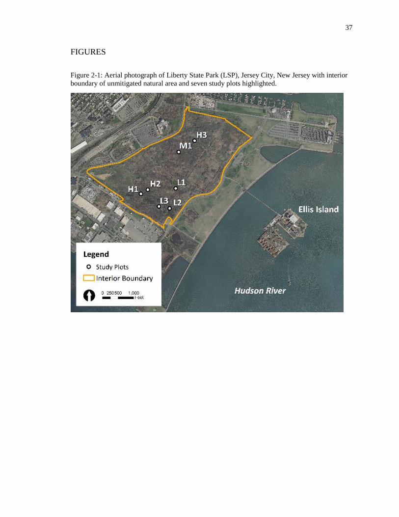
37

FIGURES

Figure 2-1: Aerial photograph of Liberty State Park (LSP), Jersey City, New Jersey with interior

boundary of unmitigated natural area and seven study plots highlighted.

38

Figure 2-2: Soil TE concentrations (mg/kg) in the C1 horizon from 1995, 2005, and 2015 for

seven study plots (n = 6, 21, and 35, respectively). Groups which share the same letters are not

statistically different (p < 0.05) according to a Tukey HSD test. Note that concentrations of all TE

are shown on a logarithmic scale.

39

Figure 2-3: Soil TE concentrations (mg/kg) in the C1 horizon from 2005 (n = 3 per plot) and

2015 (n = 5) for seven study plots. Concentrations within plots which share the same letters are

not statistically different (p < 0.05) according to a Tukey HSD test. Note that concentrations of all

TE are shown on a logarithmic scale.

40

Figure 2-4: Soil TE concentrations (mg/kg) in 2015 samples from the A, C1, and C2 horizons

measured by pXRF (n = 5 per horizon per plot). Solid triangles represent mean concentrations,

open circles represent individual concentrations.

41

Figure 2-5: Soil pH measured in the C1 horizon in 2005 (n = 7) and 2015 (n = 35) for seven study

plots.

42

Figure 2-6: Soil pH of the A, C1, and C2 horizons in 2015 (n = 5 per horizon). Solid triangles

represent mean pH, open circles represent individual pH measurements.

43

Chapter 3 - Photosynthetic rates and gas exchange parameters of

Betula populifolia growing in trace element contaminated soils

INTRODUCTION

Prior research at Liberty State Park found inverse correlations between soil trace element

concentrations and tree growth rates. Tree coring data showed that over the course of six years,

there was a significant negative curvilinear relationship between total metal load (TML, see

Chapter 1) and cumulative cross sectional trunk area added (Gallagher et al. 2008a). A second

study found significant differences in the relationships of Betula populifolia trunk diameter and

tree age between high and low metal load plots (Dahle et al. 2014). Similarly, when comparing

Populus deltoides at Liberty State Park with similar trunk diameter at high and low metal load

plots, the high metal load trees tended be older than their similarly sized low metal load

counterparts (Renninger et al. 2012).

One possible explanation for the observations of decreased growth rates in these trees is a

decrease in photosynthesis leading to a decrease in biomass production. Direct and indirect

effects of trace elements on photosynthesis are well documented. Trace elements can reduce the

production of chlorophyll, interact with enzymes such as Rubisco, change the function of

chloroplast membranes, interact with both the electron donor and acceptor components of

photosystem I and photosystem II, impair stomatal function, and interfere with the photosynthetic

carbon reduction cycle (Mysliwa-Kurdziel et al. 2004). However, all of these responses are

element and species specific. Frequently laboratory studies which were designed to investigate

interactions at a molecular level do not necessarily represent the response of the whole plant to

the concentrations of trace elements found in the environment. Plants are able to survive elevated

concentrations of trace elements using a variety of mechanisms, including active exclusion (to a

limit), isolation in vacuoles, and binding with chelating complexes and ligands (Greger 2004).

44

The interaction between trace elements and plant water relations are complex,

particularly when drought is involved. Trace elements have been shown to affect water transport

through roots (Maggio and Joly 1995), decrease the diameter and number of xylem vessels (Robb

et al. 1980), induce stomatal closure (Moustakas et al. 1997), and create a stress response which is

similar to water-deficiency stress (de Silva et al. 2012). All of these responses vary among metals

and plant species. Interestingly, some of these effects may confer drought resistance. Changes in

xylem structure, higher stomatal resistance, smaller and fewer leaves, and enhanced abscission

effectively promote water conservation by the plant, countering the effects of drought

(Poschenrieder and Barcelo 2004). However, these changes are beneficial to some species but not

others (Santala and Ryser 2009; de Silva et al. 2012).

One of the dominant hardwoods at Liberty State Park, Betula populifolia, is an early

successional species, able to colonize lower quality sites though it prefers moist, well drained

soils and is not tolerant to prolonged saturation (Wennerberg 2004). Exposure to Cu and Ni

appears to confer drought tolerance to Betula papyrifera seedlings grown in a greenhouse setting

(Santala and Ryser 2009). Since the photosynthetic and stomatal conductance rates of B.

populifolia and B. papyrifera responded similarly in a drought study (Ranney et al. 1991),

perhaps trace element exposure may enable greater drought tolerance in B. populifolia as well.

Given previous broad scale observations of primary productivity and B. populifolia basal

growth rates, I hypothesized that soil metal load is the primary limitation on leaf gas exchange

and photosynthesis parameters of B. populifolia at Liberty State Park (Hypothesis 1). I also

hypothesized that high metal load would exacerbate the effects of short heat wave and drought on

gas exchange parameters (Hypothesis 2). Additionally, I hypothesized that other soil properties

such as soil nutrients and water content would also influence gas exchange (Hypothesis 3).

Specifically, it was expected that in response to stress HML trees will have lower net

photosynthetic assimilation (Anet), transpiration (E), stomatal conductance (gs), intrinsic water use

45

efficiency (iWUE), intercellular to ambient CO2 concentration ratio (Ci/Ca), maximum

carboxylation efficiency (Vcmax), electron transport rate (Jmax), light saturated photosynthetic rate

(Amax), and quantum efficiency (φ) but higher CO2 compensation point (Γ*), light compensation

point (Icomp), and dark respiration (Rdark).

BACKGROUND Members of the Betula genus can be found throughout the Northern Hemisphere in both

boreal and temperate zones (Jarvinen et al. 2004). Many Betula species are characterized as

pioneer or colonizer species and tend to be shade intolerant. This study focuses on B. populifolia

which spontaneously colonized the abandoned rail yard at Liberty State Park. B. populifolia is not

particularly well studied, though several other members of Betula from Europe, Northeastern

Asia, and North America have been the subject of both photosynthesis and trace element studies

(Table 3-1). Phylogenetic analysis of Betula suggests the closest relatives to B. populifolia are B.

platyphylla, B. papyrifera, and B. pendula (Jarvinen et al. 2004; Li et al. 2007).

Several species within the Betula genus have been found growing at or were planted in

soils with high concentrations of trace elements, including B. populifolia in abandoned rail yards

(Gallagher et al. 2008a; Murray et al. 2000); B. pendula in coal mining spoil heaps (Frouz et al.

2008; Good et al. 1985), former industrial sites (Dickinson 2000), mine spoils (Borgegard and

Rydin 1989; Margui et al. 2007) and As contaminated soils (Gustafsson and Jacks 1995; Moreno-

Jiménez et al. 2010); B. papyrifera in forests affected by acid deposition (Landre et al. 2010); B.

alba in As contaminated mine spoils (Bleeker et al. 2002); and B. pubescens in copper mine

spoils (Borgegard and Rydin 1989). Additionally Betula pendula is a commonly planted species

for brownfield greening projects in the UK (Doick et al. 2009; French et al. 2006). However

within a species there can be a high degree of genotypic variation in the establishment and growth

46

rate responses to high metal concentrations (Gaudet et al. 2011; Good et al. 1985; Kopponen et al.

2001; Utriainen et al. 1997).

Some evidence suggests metal tolerance in Betula comes from an exclusion based

mechanism, though no precise mechanism has been identified. Denny and Wilkins, (1987)

hypothesize that Betula tolerance of Zn lies in its ability to exclude Zn uptake at the root

endodermis based on their observations of a threshold type response by B. pendula and B.

pubescens to increasing Zn concentrations, excluding it up to a point then becoming inundated by

it. This work was also supported by Kopponen et al., (2001) who found that clones of B. pendula

and B. pubescens with the greatest reduction in growth when grown in Cu and Zn contaminated

soils tended to have the highest aboveground concentrations of the two elements. However, at

Liberty State Park B. populifolia and Populus deltoides have both been observed to

hyperaccumulate Zn in their leaves (Qian et al. 2012).

Betula species have been shown to tolerate exposure to elevated levels of several trace

elements and in some situations accumulating some of the elements in high concentrations.

Elevated concentrations of Cd and Cu have been documented in B. papyrifera (Landre et al.

2010) as well as high concentrations of Cd, Pb, and Zn in B. pendula and B. pubescens

(Borgegard and Rydin 1989). Though in contrast B. pendula had the lowest concentrations of Cu

in aboveground biomass (leaves and stem) compared to other species of trees (Alnus and Salix

spp.) in a brownfield afforestation study (Dickinson 2000). Betula spp. may be more resistant to

As uptake since wild growing Betula pendula at an abandoned mine site had the lowest transfer

and bioaccumulation factors (ratio of shoot to soil concentrations) for As of the woody species

sampled by the study (Moreno-Jiménez et al. 2010). For B. populifolia growing at Liberty State

Park, Zn hyperaccumulates in the leaf (as evidenced by a leaf-soil bioconcentration factor greater

than 1) while As, Cr, and Cu had much lower bioconcentration factors in the leaf (Qian et al.

2012).

47

Little field research has been conducted exploring the responses of photosynthesis in

Betula to trace element exposure. Hydroponically grown seedlings of Betula ermanii were able to

maintain relatively high net assimilation, carboxylation efficiency and quantum yield when

exposed to increasing concentrations of manganese (Kitao et al. 1997). In an open top chamber

experiment, exposure to soil contaminated with Zn, Cu, and Cd laden filter dust reduced the

evapotranspiration rates of a community of forest plants which included Betula pendula (Menon

et al. 2005); presumably such a reduction in evapotranspiration would correlate with a reduction

in net photosynthetic assimilation of CO2 as well.

In addition to toxic effects from elevated levels of trace elements in degraded sites,

frequently poor soil conditions such as low nutrient availability can also limit plant growth in

these environments. Consequently there is a strong interest in understanding the role soil

amendments may play in both negating the effects of metal toxicity as well as enabling improved

plant growth (Kumpiene et al. 2008). The application of fertilizer on study plots in opencast coal

sites did little to influence the growth of B. pendula and B. pubescens (Good et al. 1985).

However B. aurata (a pioneer species) planted in slate rock waste tips did exhibit increased

growth rates in response to the addition of clay and organic waste (Williamson et al. 2011).

Williamson et al., (2011) suggest amendments must address both water holding capacity and

nutrient availability in concert in order to be effective. The addition of lime and fertilizer

enhanced root growth of B. populifolia at the study site (Gallagher et al. 2015).

METHODS

Study Site

Study plots (20 x 50 m) were located in the interior area of Liberty State Park, Jersey

City, New Jersey (40o42’16” N x 74o03’17” W). The site was formerly a rail yard and industrial

48

area built on filled tidal marsh. The site’s history resulted in concentrations of trace elements (TE)

that exceed background levels and both residential and ecological screening criteria (New Jersey

Department of Environmental Protection 1999; United States Environmental Protection Agency

2003). Contamination varies spatially over the site which facilitates the comparison of trees

growing in both high and low concentrations of TE. Plots within Liberty State Park have been

compared using a rank composite index based on soil concentrations of As, Cr, Cu, Pb, and Zn

called the total metal load index (TML, See Chapter 1).

This study focused on four hardwood plots at Liberty State Park, two with soils below a

previously defined critical TML threshold of 3 (Gallagher et al., 2008) and two above the

threshold (Table 3-2). All four study plots were located in early successional hardwood stands

which are predominantly composed of Betula populifolia along with Populus deltoides and

Populus tremuloides.

Gas Exchange measurements

Measurements of leaf gas exchange were made monthly from May to September in 2014

and 2015. Within each of the four plots, five mature B. populifolia trees were selected based on

their diameter at breast height (DBH) to ensure individuals represented the 2nd to 4th DBH

quartiles previously determined for the population (Dahle et al. 2014). When possible, the same

trees were measured from month to month, however some trees had to be cycled out of the study

due to deteriorating conditions in canopy (high number of dead branches). All measurements

were made on excised branches collected from approximately 5 m above the ground, which were

immediately placed in water and recut while submerged to maintain a hydraulic connection for

the leaves (Joesting et al. 2009; Kubiske and Pregitzer 1996; Reich et al. 1995). Preliminary

excision experiments at Liberty State Park in 2014 showed the excision procedure did not

influence photosynthesis rates.

49

To quantify leaf photosynthetic traits, two sets of gas exchange measurements were made

typically between the hours of 8:00 and 13:00, using a LI-COR 6400XT portable gas exchange

system (LI-COR Biosciences, Lincoln, Nebraska). These were made using the first and second

fully expanded leaves (i.e. most apical and second-most apical) with minimal damage on each

excised branch. For the first set, light availability measured as photosynthetic active radiation

(PAR) was varied from saturating to darkness using the instrument’s LED chamber. These “light

curves” were generated using the following photosynthetic photon flux density (PPFD) sequence:

2000, 1500, 1000, 500, 200, 100, 50, 20, 0 μmol photons m-2 s-1. During these measurements

reference CO2 was maintained at 400 μmol CO2 mol-1 air. The second set of measurements, “A-

Ci” curves, maintained constant saturating light at 1500 μmol photons m-2 s-1 and varied ambient

CO2 concentrations using the following sequence: 400, 300, 200, 100, 50, 400, 400, 600, 700,

800, 900, 1000, 1500 μmol CO2 mol-1 air. Relative humidity in the sample chamber was

maintained between 60 and 80% and chamber temperature was set to 25oC for both sets of

measurements.

To determine if soil metal loads compounded or increased the effects of high

temperature, an additional set of A-Ci curves were collected on July 25 and 26, 2014 Five trees

from high metal plot H3 and five trees from low metal plot L1 were used in the temperature study

(none of these trees were used in the primary study). Temperature was controlled by setting the

LI-6400 block temperature to 25, 30, and 35oC (note that the highest leaf temperature achieved

was 34.4oC). A different branch was excised for each temperature level and acclimated in the

cuvette until readings stabilized. All other settings for the A-Ci curves were the same as the

procedures described above.

Three days of high temperatures (19-21 July 2015) occurred in the middle of the

sampling period; daily maximum temperatures ranged from 33 to 36oC. A total of 1.8 cm of rain

had fallen in the preceding two weeks and daily reference evapotranspiration (ETo) ranged from

50

1.3 to 4.7 mm day-1 on these three days (see Weather Data subsection for explanation of ETo

calculation). Preliminary measurements made on July 21 indicated photosynthetic rates were

much lower than normal. Consequently additional survey measurements – single gas exchange

measurements – were made on July 22 and 23 (daily maximum temperature 30oC, ETo 8.7 and

8.3 mm day-1) in order to capture net photosynthetic assimilation (Anet), transpiration (E), and

stomatal conductance (gs) from all of the study trees in a short amount of time.

Survey measurements were made on leaves of excised branches at 400 μmol CO2 mol-1

air and 1500 μmol photons m-2 s-1. A leaf was placed in the sample chamber, then once CO2 and

H2O concentrations stabilized a single measurement was made. While there is no single agreed

upon definition of a heat wave (Smith et al. 2013), the July 19-21 period of high heat dry weather

will be referred to as the July 2015 heat wave for the purposes of this paper.

Leaf mass per unit area (LMA) was measured for all leaves used in gas exchange

measurements in 2015. Leaves were scanned using an Epson Expression 11000XL scanner then

the leaf area was measured using ImageJ (imagej.nih.gov/ij/) software. Leaves were oven dried at

60oC for at least 72 hours then cooled in a desiccator and weighed. LMA was calculated by

dividing the leaf dry weight (g) by the leaf area (m2).

Soil properties

To compare soil properties other than heavy metals across the study plots, 3 to 4 samples

were collected from random location within each study plot using a slide corer from the top 15

cm of soil (excluding intact leaf litter). The < 2 mm fraction of the soil samples were analyzed by

the New Jersey Agricultural Experiment Station (NJAES) Soil Testing Lab for pH, soil texture,

electrical conductivity, macro and micronutrients. pH was measured using a 1:1 ratio of soil to

liquid (by volume) with S975 SevenExcellence Multiparameter pH meter (Mettler Toledo,

Columbus, OH). The hydrometer method was used to determine soil texture with 50 g of soil (<2

51

mm) dispersed with 50 mL of 10% Na-Hexametaphosphate. Total Kjeldahl Nitrogen (TKN) for

total organic nitrogen plus free ammonia was determined following EPA Method 351.1 using an

AutoAnalyzer III (wavelength = 667 nm, Bran + Luebbe Analytics, Norderstedt, Germany).

Macro and micronutrients (P, K, Ca, Mg, Zn, Mn, Cu, B, and Fe) were extracted using a Mehlich-

3 extractant and analyzed using an iCAP 7000 inductively coupled plasma optical emission

spectrophotometer (ICP-OES; Themo Scientific, Waltham, MA). Note that the Mehlich-3

extractions approximate plant available element concentrations rather than total or pseudo-total

concentrations.

Gravimetric soil water content (θg) was measured in the four study plots at the beginning,

middle and end of each monthly photosynthesis measurement period in 2015. There were three

sample locations in each plot which were sampled repeatedly over the course of the growing

season. When possible, all four plots were sampled on the same day. Samples were collected with

a core sampler or auger from the top 15 cm of the soil profile and were dried in an over at 110oC

for a minimum of 3 days until they reached constant mass. θg was calculated as,

W Dg

D

M M

M

(1)

where MW and MD are the masses of the soil before and after drying, respectively.

Weather Data

Hourly and daily weather data (temperature, relative humidity, wind speed, and

precipitation) for the study period was collected at a weather station at Liberty Science Center,

Jersey City, NJ (Station #3411) next to the site (New Jersey Weather & Climate Network 2016).

Reference evapotranspiration (ETo) was calculated using the Penman Monteith equation

following the procedure outlined by the Food and Agricultural Organization (FAO):

52

86,400

1

s a

N a p

a

s

a

e eR G C

rETo

r

r

(2)

Where Δ is the rate of change for saturated vapor pressure change (kPa oC-1), RN is net radiation

at the crop surface (MJ m-2 day-1), G is soil heat flux (MJ m-2 day-1, assumed negligible for single

day time step), ρa is mean air density (kg m-3), Cp is the specific heat of air at constant pressure

(MJ kg-1 oC-1), es is saturation vapor pressure (kPa), ea actual vapor pressure (kPa), ra is

aerodynamic resistance (s m-1), λ is the latent heat of vaporization (MJ kg-1), γ is the

psychrometric constant (kPa oC-1), and rs is the surface canopy resistance (s m-1). Aerodynamic

resistance (ra, s m-1) was calculated according to:

2

ln lnm h

om om

a

z

z d z d

z zr

k u

(3)

Where zm is the height of wind measurements (10 m), zh is the height of the humidity

measurements (10 m), zom is the roughness length governing momentum transfer (m), zoh is the

roughness length governing transfer of heat and vapor (m), d is the zero plane of displacement

height (m), k is von Karman’s constant (0.41, no units), and uz is wind speed at height z (m s-1).

As recommended by FAO, the equations for calculation for a hypothetical reference crop with an

assumed height of 0.12 m, fixed surface resistance (rs) of 70 s m-1 and an albedo of 0.23 (Allen et

al. 1998). For this purpose, ETo is intended to represent the atmospheric demand for water, not

actual ET.

53

Data Analysis

Light curves were fitting using nonlinear least squares regression utilizing a procedure

described by Lobo et al. (2013). Since several different equations are available for fitting light

curve data to determine leaf photosynthetic traits or parameters, Lobo et al. (2013) suggest fitting

data with multiple equations and then selecting the equation which produces the lowest sum of

squares of the errors. The following equation from Prioul and Chartier (1977) was found to

produce the best fit for the greatest number of light curves collected for the study:

2

( ) max ( ) max ( ) max4

2

Io g Io g Io g

N dark

I A I A I AA R

(4)

Equation parameters and their abbreviations are described in Table 3-3. The maximum

assimilation rate (Amax) was determined from net assimilation (Anet) in saturating light at the

irradiance level (I) above which no significant change in Anet occurred. The light compensation

point (Icomp), the irradiance at which CO2 assimilation and respiration are equal, was calculated

from the parameterized equation by setting Anet equal to zero. Quantum yield (φ, also called

quantum efficiency) was taken as φ(Io) in Eq. 4. While both are measured at ambient CO2 and

saturating light conditions, Amax and Anet are treated separately since Amax is calculated based on

light curves and Anet is a direct measurement point which was made both while collecting curve

data and single survey measurements.

A-Ci curves were fit according to the Farquhar-Von Caemmerer-Berry (FvCB) model of

C3 photosynthesis (Farquhar et al. 1980). The FvCB model splits the A-Ci curve into two or three

regions. The low Ci (intercellular CO2) portion of the curve (< ~400 ppm) represents Rubisco

limited photosynthesis which is described by:

max

*

1 /

iC c D

i C O

CA V R

C K O K

(5)

54

The high Ci portion of the curve (> ~ 400 ppm) represents RuBP regeneration limited

photosynthesis:

*

4 8 *

iJ D

i

CA J R

C

(6)

At very high Ci, photosynthesis can additionally become limited by triose phosphate use (TPU):

3P DA TPU R (7)

At a given Ci net photosynthetic assimilation (Anet) is a function of the most limiting process:

min , ,N C J PA A A A (8)

Equation variables and their units are listed in Table 3-3. Values of Γ*, KO and KC were based on

Bernacchi et al. (2001) and were temperature corrected using the following version of the

Arrhenius equation:

( )

aHc

R TleafParameter e

(9)

where Tleaf is the leaf temperature in Kelvin and R is the universal gas constant (8.314 J mol-1 K-

1). Values for c (a scaling constant) and ΔHa are shown in Table 3-4, based on Bernacchi et al.

(2001, 2003).

A-Ci curves were fitted to parameterize maximum carboxylation rate (Vcmax), maximum

electron transport rate (Jmax), triose phosphate utilization (TPU), and dark respiration (Rdark) using

the plantecophys package in R statistics run in the R computing environment (Duursma 2015; R

Core Team 2016). One challenge in fitting A-Ci curves is identifying the level of Ci where one

limitation transitions to another (the Ci transition point), especially since at some concentrations

both Rubisco and RuBP regeneration can be co-limiting (Sharkey et al. 2007). The plantecophys

package obviates the need to manually determine the Ci transition point for each curve and has

two options for fitting the FvCB model. For curves which were not TPU limited, the program’s

default non-linear regression approach was used. Curves with all three limitations were fit using

55

the program’s linear method. If a curve had less than three points available to constrain the RuBP

regeneration or TPU limited equations, Jmax and/or TPU were be excluded from further analysis.

To facilitate comparison, Vcmax and Jmax were normalized to 25oC using the constants shown in

Table 3-4. While the temperature response constants for KC, KO, and Γ* are considered intrinsic

properties of Rubisco and are fairly well conserved among species (von Caemmerer 2000),

Medlyn et al. (2002) show that there can be greater variability in the temperature responses of

Vcmax and Jmax, even within species. While temperature response data for A-Ci curves was

collected as part of the study, the temperature range was not wide enough to accurately estimate c

and ΔHa for B. populifolia at LSP. The values of c and ΔHa used in this study do fall well within

the range of values found by Medlyn et al. (2002) for deciduous trees. All of the other default

settings in plantecophys were used for fitting. The CO2 compensation point (Γcomp) was calculated

by solving the fitted model for Anet = 0.

Intrinsic water use efficiency (iWUE, also called potential water-use efficiency or

physiological water-use efficiency) was calculated as

/net siWUE A g (10)

Where Anet and gs are the net photosynthetic assimilation rate (μmol CO2 m-2 s-1) and stomatal

conductance to water vapor (mol H2O m-2 s-1) at 400 ppm CO2 and 1500 μmol PPFD m-2 s-1.

Statistical Analysis

Photosynthesis parameters were tested using a linear mixed effects model. The effects of

metal load (ML) and sample month and year (MY) on each photosynthesis parameter were tested

using a linear mixed effects model. The low metal load group included plots L1 and L2 while the

high metal load group included plots H2 and H3. Linear mixed effects models account for within-

subject or within-group variation by setting random intercepts for each individual and/or cluster.

56

ML, MY and their interaction were treated as fixed effects while tree and plot were treated as

random effects. Three models were tested for each parameter: 1) the full model (ML and MY plus

their interaction), 2) ML only, and 3) MY only. Jmax, Γcomp, Icomp, E, and gs were natural log

transformed to achieve normality and constant variance of residuals. Likelihood ratio tests were

used to determine the significance of ML, MY and their interaction by testing each of the three

models against a null model containing only random effects.

The relationship between A-Ci curve parameters and leaf temperatures from the

temperature response study was tested using linear regression with an interaction effect between

leaf temperature and metal load (LML or HML). Leaf conductance (gs) and E were log

transformed in order to normalize their residuals. To facilitate interpretation of the linear

regression intercept coefficient (which would be 0oC and meaningless in this context) leaf

temperature was re-centered on the mean temperature, 30oC, prior to running the regression.

Using the re-centered leaf temperatures, the intercept coefficient represents the mean value of a

parameter for the low metal load (LML) trees at 30oC. The high metal load (HML) coefficient is

then the difference between the LML mean and the HML mean at 30oC.

The effects of weather variables on the photosynthesis parameters were tested using

linear and quadratic regressions. Since all measurements were made in the morning, daily

maximum and mean temperatures as well as precipitation were based on the 24 hours preceding

the morning of the measurement. Precipitation totals were also calculated for the 72 hours

preceding the morning of the measurement. For both types of regression photosynthesis

parameters were tested for normality and constant variance and were transformed as needed.

However no suitable transformation was found for the light compensation point, stomatal

conductance, and quantum yield consequently those parameters were excluded from this analysis.

One way ANOVAs were used to compare soil water content (θg) between plots on each

day soil samples were collected to determine if θg varied significantly between plots. Residuals

57

were normally distributed and had constant variance so no transformations were needed. On dates

when the ANOVA indicated a significant difference between plots, a Tukey HSD test was used to

assess which plots were significantly different from the others. A linear mixed effects model was

also used to test the interacting effects of metal load and θg using plot and tree as random effects.

On days when photosynthesis was measured but θg was not, θg was estimated by linearly

interpolating between the two closest θg measurement dates.

RESULTS

Photosynthesis parameters varied strongly by measurement month-year (MY), but did not

show strong differences based on soil metal load (ML) alone – no parameter had a significant ML

only model (Table 3-5). There was greater variance between trees than between plots, though

within subject variation for all parameters was at least an order of magnitude greater than the

variance from either random effect (Table 3-6). However significant interactive effects between

MY and ML for were observed for maximum carboxylation rate (Vcmax), electron transport rate

(Jmax), quantum efficiency (φ), light compensation point (Icomp) and intrinsic water use efficiency

(iWUE) (Table 3-7). In July 2014 and May 2015, Vcmax, Jmax, and φ were significantly lower for

high metal load trees compared to low metal trees1 (Figure 3-1). Vcmax and φ were also

significantly lower for high than low metal load trees in September 2014 as was Jmax in August

2014 and June 2015. Following the heat wave in July 2015, the iWUE of high metal load trees

was significantly lower in that month.

1 Note that the rephrasing “low metal” and “high metal trees” refers to trees growing in soils with a respectively low or high total metal load (TML) and does not necessarily mean the tree has a high concentration of metals

58

Though metal load alone was not a significant predictor of any of the photosynthesis

parameters, several trends suggest that the high metal load trees were under stress (Figure 3-2).

The medians of Vcmax, Jmax, maximum net assimilation (Amax), light compensation point (Icomp),

quantum efficiency (φ), dark respiration rate (Rdark), and net assimilation (Anet) were all lower in

the high metal load trees while CO2 compensation point (Γcomp), and iWUE were higher. The

medians of transpiration (E) and stomatal conductance (gs) were not different between metal load

though the high metal 3rd and 4th quartiles are lower. These results do not provide strong evidence

in support of Hypothesis 1 and instead highlight the strong seasonal variation in the

photosynthetic physiology of these trees.

Leaf mass per area (LMA) was the only parameter with a significant metal load (ML)

only model which indicated that the mean LMA from the low metal load trees (53 ± 1 (standard

error) g m-2) was significantly greater than the mean of the high metal load trees (47 ± 2 g m-2).

While LMA of the 2015 leaf samples ranged from 11 to 88 g m-2, the low standard deviation (9.3

g m-2) about the mean of all samples (49.9 g m-2) suggests that overall LMA was fairly consistent

among the sample leaves. Other authors have found LMA for B. populifolia leaves ranging from

74 to 95 g m-2 (Chen et al. 2014; Wayne and Bazzaz 1993).

Monthly temperature and precipitation in 2014 were similar to statewide historic monthly

averages, although precipitation in August, September, and October 2014 were about 5 to 6 cm

below statewide historic averages (Figure 3-3, Table 3-8). During the 2014 growing season mean

assimilation values (Amax and Anet) peaked in June while the maximum carboxylation rate (Vcmax)

for low metal trees peaked in July (Figure 3-1). Quantum efficiency (φ), light compensation point

(Icomp), and dark respiration (Rdark) means were also low in July 2014. Intercellular to ambient CO2

ratio (Ci/Ca), transpiration (E), and stomatal conductance (gs) decreased from May to August

2014 while CO2 compensation point (Γcomp) and intrinsic water use efficiency (iWUE) increased.

July through September 2015 were both hotter and drier than the statewide historic average, with

59

July and August both having very low precipitation totals (Figure 3-4). ETo did not vary greatly

between the two study seasons.

While June 2015 was wetter than average, a short heat wave (several days of high

temperatures and no rainfall) in July 2015 strongly affected photosynthesis parameters. The point

sample measurements from the L1 trees suggest that before the heat wave, photosynthesis rates

were comparable to rates in 2014 (Figure 3-5). However 3 days after the start of heat wave net

assimilation (Anet), transpiration (E), stomatal conductance (gs), intercellular CO2 (Ci), and

intercellular to ambient CO2 ratio (Ci/Ca) in plot L1 all decrease dramatically while iWUE

increases. Additionally in the remainder of the plots measured in the days following the heat

wave, maximum carboxylation rate (Vcmax), net assimilation (Amax and Anet), quantum efficiency

(φ), dark respiration (Rdark), transpiration (E), and stomatal conductance (gs) were all much lower

in July 2015 compared to July 2014 (Figure 3-1). CO2 compensation point (Γcomp) and intrinsic

water use efficiency (iWUE) were much higher in July 2015 compared to 2014. In August 2015

Vcmax, Amax, φ, and Rdark remained low while Anet, E, and gs increased slightly and increased again

in September to similar levels observed in 2014.

Following the initial hypothesis, the high metal load trees had lower mean iWUE in July

2015 after the heat wave compared to low metal load (Figure 3-6, Table 3-7). iWUE declined for

both groups in August and September 2015 as gs rates increased but Anet remained fairly low.

High metal load transpiration and gs were lower in August 2015, which was 7 cm drier than the

statewide historic average, but were higher compared to low metal load trees in September 2015.

The relationship between gs and Ci/Ca can be used to separate the effects of stomatal and

non-stomatal limitations on photosynthesis during periods of water stress (Brodribb 1996; Singh

and Raja Reddy 2011). For most of the study months, the relationship between gs and Ci/Ca

follows an expected exponential rise to maximum function where higher Ci/Ca is associated with

higher gs but is not affected by metal load (Figure 3-7). However while some measurements show

60

a very sharp decline in Ci/Ca with decreasing gs, other measurements made in July and August

2015 show that Ci/Ca increases drastically at very low gs. These observations of very high Ci/Ca at

very low gs, which occurred in all four study plots, strongly suggest the occurrence of non-

stomatal limitations to photosynthesis in these trees (Brodribb 1996).

Amax, Anet, Icomp, Rdark, Vcmax, and E all had significant relationships with weather variables

though all of the model fits are fairly weak (Table 3-9). All of the polynomial regressions for

temperature reach a maximum around 15oC for both maximum and mean daily temperature

(Figure 3-8). E and Anet had negative relationships with ETo. Rdark was predicted by both

temperature and precipitation. Both 24 and 72 hour precipitation totals predicted Anet, Icomp, and

Rdark with either a positive linear relationship or a polynomial relationship which reached a

maximum around 2 cm (72 hours) or 1 cm (24 hours).

Varying leaf temperatures from 25 to 35oC altered photosynthesis parameters though no

interactive effects with metal load were observed, i.e. metal load did not change the relationship

between the parameters and leaf temperature. There were significant relationships between leaf

temperature and Vcmax, Jmax, Γcomp, gs (log transformed), and Ci (Table 3-10). However

assimilation and transpiration were not significantly affected by leaf temperature. Positive

relationships were observed for Vcmax, Jmax, and Γcomp, while the other significant parameters

decreased with increasing temperature (Figure 3-9). Jmax values from high metal load trees were

significantly lower than those from the low metal plot at 30oC though there were no interactive

effects between metal load and leaf temperature. None of the other parameters were significantly

affected by metal load. However all high metal load coefficients indicate that the mean value for

high metal load trees at 30oC were lower than the low metal means.

Some differences were observed between the macro and micronutrients and other soil

properties of the four study plots (Tables 3-11, 3-12, 3-13). For the most part macronutrient

concentrations were similar for the high and low metal load plots, though interestingly L2 and H3

61

had similarly low phosphorus concentrations in comparison to L1 and H2. Concentrations of

Mehlich 3 extractable Zn and Cu were significantly higher in Plot H3 compared to plots L2 and

H2.

Gravimetric soil water content (θg) in all four plots declined from ~45% to ~10% over the

course of the 2015 study period (Figure 3-4) which coincides with the decreasing rainfall from

June to September 2015. In June and July 2015 L2 tended to have the highest and L1 the lowest

θg, while H3 and H2 had fairly similar intermediate θg values. In August 2015, θg in L2 had

decreased to a similar level as H3 and H2 and by September θg from all four plots had converged.

According to Tukey HSD tests, θg was significantly higher in L2 compared to L1 on 2015-07-14

and 2015-07-21. No significant differences were found between the plots for any of the other

measurement days. Net photosynthesis (Anet), E, and gs scaled positively with θg for

measurements made from June to September 2015 (Table 3-14, Figure 3-10). Interactions

between θg and metal load were observed for Vcmax, Rdark, and Amax. In general these parameters in

the low metal group were less sensitive to decreasing θg. This apparent lack of sensitivity seems

to be driven by Plot L1 (Figure 3-10) which tended to have the lowest θg yet higher Vcmax, Amax,

and Rdark values compared to the high metal load trees at similar θg.

DISCUSSION

Hypothesis 1: Soil metal load is primary limitation on photosynthesis parameters

The effects of soil metal load on the photosynthesis parameters of B. populifolia trees

growing in LSP were not as drastic as initially hypothesized. Numerous studies have

demonstrated that photosynthesis and related gas exchange parameters are diminished with

increasing exposure to a variety of heavy metals (e.g. Di Baccio et al. 2009; Gaudet et al. 2011;

Pereira et al. 2016; Santana et al. 2012). Differences in methodologies and reporting make it

extremely difficult to compare soil trace element concentrations across studies. Consequently it is

62

possible that the gradient of trace elements in the LSP study plots was not as wide as those

assessed in other studies which may account for the smaller differences observed in this

photosynthesis study. A large body of research on the effects of heavy metals on plants and

photosynthesis has been conducted in lab or greenhouse settings in which leaves and chloroplasts

were exposed to metal solutions directly or plants were grown in media with high bioavailable

concentrations (Mysliwa-Kurdziel et al. 2004). While these approaches are valuable for

elucidating mechanistic responses, they do not reflect complex field conditions where many

interacting factors may mediate leaf level TE response, including community level interactions

(Krumins et al. 2015) and plant-mycorrhizal associations (Yang et al. 2015).

One of the few significant metal load month-year interactions – the significant decreases

in Vcmax and Jmax in July 2014 and May 2015 – could be the result of elevated Zn concentrations in

the leaves during these time periods. Gallagher et al. (2008) found B. populifolia leaf Zn

concentrations changed over the course of the growing season and that in HML plots there were

significant positive relationships between leaf Zn and leaf red/green ratio index (an image-based

proxy for chlorophyll content). Amax and Anet also decreased in the HML trees during these two

months, though their decreases were not significant. HML Rdark was also lower in this month,

potentially offsetting the effects of reduced Vcmax and Jmax on net assimilation rates. While these

reductions may be transient, it is possible that they occur during a critical part of the year and had

substantial effects on overall growth rates (Boone et al. 2004). The significantly lower Vcmax and

Jmax observed in HML trees in July 2014 and May 2015 suggest metal stress effects may be

transient and seasonal.

The decreasing trend of Vcmax, Jmax, Amax and Anet with metal load has been observed for

many species as a stress response with exposure to various metals (e.g. Van Den Berge et al.

2011; Gaudet et al. 2011; Pereira et al. 2016). The mean value of Anet measured at LSP during

2014 (the average growing season), was lower than mean values for Betula species from other

63

sites found in the literature review (Table 3-1). The 2014 means of Vcmax, Jmax, and gs were all less

than the literature values. Rdark and Icomp means were within the literature range while φ was

slightly higher. While study conditions and methods do influence gas exchange measurements,

the tendency of several photosynthetic parameters measured at LSP to be less than those from

other locations suggests the photosynthetic capacity of the LSP trees may be limited in

comparison to trees growing in non-contaminated soils. These lower rates could be attributed to

stress from exposure to TE and/or the sub-optimal availability of some macro- and micro-

nutrients observed in the study plots. Lack of nutrient availability and low water availability are

common in degraded and anthropogenic soils and can hinder restoration efforts (Williamson et al.

2011; Wong 2003).

It was initially hypothesized that Rdark would increase with increasing TML similar to the

results of other studies which posited higher Rdark indicates increased ion export rates and/or

increased production of metal-binding molecules (Losch 2004; Romanowska et al. 2002; Vassilev

et al. 1997). At LSP, Rdark tended to be lower in the HML group suggesting that leaves from these

trees were not spending much additional energy on protection mechanisms against TE. Similar

results were observed by Hermle et al. (2007) for Salix vinimalis and Populus tremula grown in

soil contaminated with smelter dust. The decrease in Rdark can instead be attributed to the

concurrent lower rate of Amax (and Anet) which means less substrate is available for respiration

(Cannell and Thornley 2000). Given the lower rates of Rdark observed in the leaves from high

metal load trees, evidence is lacking for a strong protection response by these B. populifolia

leaves.

As expected, an increase in Γcomp was observed in the high metal load (HML) trees. High

Γcomp can indicate an increase in photorespiration – the release of CO2 during photosynthesis

when O2 rather than CO2 binds to RuBP (Di Baccio et al. 2009). Photorespiration can increase as

stomatal closure limits CO2 supply, or it may also increase to reduce the effects of other stresses

64

(Wingler et al. 2000). HML gs rates are in the lower range compared to low metal load (LML), an

effect which is also manifested in the lower Ci/Ca and higher iWUE in the HML trees. This

reduction in HML gs makes it difficult to determine how much of the increase in Γcomp is a direct

result of stomatal limitation or of a stress response to elevated TE concentrations in the leaf.

TE exposure can affect plant-water relations in many ways, including causing ion

imbalance, disrupting hormone signaling, or causing structural changes in water transport

pathways (Poschenrieder and Barcelo 2004). Yet surprisingly when compared as an entire group,

few differences were observed in E and gs between HML and LML leaves though iWUE was

higher for HML trees. Variable responses of iWUE to heavy metals have been reported in the

literature. In some cases iWUE decreases with increasing metal exposure which is usually

attributed to a reduction in net photosynthetic rates (Anjum et al. 2016; Hermle et al. 2006;

Stancheva et al. 2014), while in other cases iWUE increased with increasing metal exposure

usually because stomatal conductance has decreased (Nwugo and Huerta 2008; Stancheva et al.

2014). While both Anet and gs are generally lower in the HML trees, it appears the increasing

iWUE reflects a greater decrease in gs. Other studies have observed correlations between reduced

root biomass and rooting depth and reduced gs which then increased iWUE (Köhler et al. 2016;

Menon et al. 2007). The higher iWUE in HML trees at LSP may reflect greater water stress

caused by metal exposure as well as a potential for different root responses in HML soils.

Since net carbon assimilation is fairly similar between the low and high metal groups,

differences in whole plant growth and community productivity observed by previous research at

the site could result from differences in carbon allocation between low metal and high metal load

trees. Exposure to TE can alter patterns of biomass allocation within plants, though in some

species allocation to below-ground biomass is favored (Brun et al. 2003; Zhang et al. 2014) while

others increase allocation to above-ground or reproductive resources (Sánchez Vilas et al. 2016).

Notably different mycorrhizal communities and soil enzymatic rates have been observed in other

65

study plots within LSP (Evans et al. 2015; Hagmann et al. 2015) suggesting that facilitative

interactions with soil biota may also play an important role in tree growth in this site.

Leaf mass per area (LMA) in 2015 was the only measured parameter with a significant

metal load only model. The decrease in LMA with increasing metal load could be an indication

that the high metal load trees preferentially allocate resources to other compartments, such as

roots. Alternatively since lower LMA is associated with shorter leaf longevity (Wright et al.

2004), the lower LMA in the high metal load (HML) trees may result from higher leaf turnover

rates in these trees, which would also divert carbon from trunk biomass. Lower LMA can

represent a decrease in the resources allocated to a leaf because of a change in leaf thickness

and/or the concentrations of cellular compounds (Poorter et al. 2009). Some studies have found

LMA to respond to metal exposure (Di Baccio et al. 2009; Renninger et al. 2015) while others

found no effect (André et al. 2006; Shi and Cai 2009) or species specific effects (Hermle et al.

2006). Light availability is a strong driver of LMA variability within an organism or species

(longer exposure to light leads to greater LMA), though LMA can also be influenced by water

availability and salinity stress (Poorter et al. 2009). Other authors have found LMA for B.

populifolia leaves ranging from 74 to 95 g m-2 (Chen et al. 2014; Wayne and Bazzaz 1993) which

is at the upper range of leaf samples measured at LSP in 2015 (11 to 88 g m-2) which suggests

that LMA is negatively affected by exposure to TE even in the low metal load trees.

Hypothesis 2: Elevated ML will exacerbate effects of stressful weather

While there is evidence that heat response proteins confer protection of photosynthetic

pathways from heavy metals (Heckathorn et al. 2017) and that plants exposed to heavy metals

may have greater thermotolerance (Howarth 1990), it is also possible that heat and metal stress

may produce an additive negative effect on photosynthesis. Between the ranges of 25 to 35oC, no

differences were observed in the relationships between leaf temperature and photosynthetic

66

parameters from the high metal (HML) and low metal load (LML) trees. It is possible that within

this temperature range leaves were either not exposed to heat for a long enough period of time to

induce heat shock or that higher temperatures were needed to induce a response. Within this

range of temperatures and exposure time, the increasing Vcmax and Jmax suggests little to no

thermal damage occurred. However a concurrent increase in Anet was not observed since gs

declined in response to higher temperatures.

The invariant Anet across a temperature range of 25 to 35oC observed for LSP B.

populifolia is similar to temperature responses observed in studies of other Betula species. B.

papyrifera, B. pendula, B. jacquemontii, and B. nigra had optimal temperatures for Anet ranging

between 25 and 30oC (Ranney and Peet 1994). Another study found B. papyrifera’s optimal Anet

temperature to be 24oC in a mixed deciduous stand in Michigan (Jurik et al. 1988). Optimal

temperatures for B. platyphylla tended to be lower, 25oC in a common garden experiment in

North Carolina (Ranney and Peet 1994) and 10 to 20oC in Hokkaido, Japan (Koike and Sakagami

1986). An optimum temperature for Vcmax and Jmax was not observed in the temperature range of

this study which is consistent with findings for B. pendula which had optimal temperatures at

37.9 and 35.1oC, respectively (Dreyer et al. 2001). At LSP, B. populifolia grows both at the

southern end of its range and at a low altitude. The results of the temperature analysis and survey

measurements following a heat wave suggest this population may be sensitive to higher

temperatures and dry conditions as would be expected for its genus.

As more extreme weather events are expected in the coming century under various

climate change scenarios, it is important to understand the ways abiotic soil stressors can interact

with extreme weather events. During the July 2015 heat wave, while slightly above average

temperatures occurred for only three days when temperatures decreased, ETo actually increased

because of sunnier weather and θg measurements in three of the four plots continued to decrease

in the following days. These conditions, while not particularly remarkable in the context of

67

regional weather trends, dramatically reduced photosynthesis rates for a period of several days.

The positive relationships observed between soil water content and net photosynthesis,

transpiration and conductance strongly suggests lack of water was an important driver for the

reduction of photosynthesis rates in the second half of the 2015 growing season. The leaf

temperature study suggests that while this population of B. populifolia is somewhat sensitive to

this temperature range, it was probably the combination of elevated temperature plus the lack of

antecedent rainfall and higher evaporative demand that produced the observed decline. In a study

of mild drought stress on six birch species, B. populifolia, was moderately affected by lack of

water in comparison with the other species (Ranney et al. 1991). A decrease in soil water content

of potting mix from 45% to 10% effectively halved Anet of B. populifolia (Graves et al. 2002).

Similarly imposition of a water deficit reduced B. papyrifera Vcmax by 46% (Gu et al. 2008).

The lower iWUE observed for the high metal load (HML) trees after the July 2015 heat

wave and in August 2015 suggests the HML trees are more negatively affected by heat wave.

There is a mix of reports on the interacting effects of trace elements and water stress on plant

growth. Some researchers have suggested that metal induced changes in xylem structure, higher

stomatal resistance, smaller and fewer leaves, and enhanced abscission effectively promote water

conservation by the plant, countering the effects of drought (Poschenrieder and Barcelo 2004). In

a pot experiment, the dry mass of B. papyrifera seedlings exposed to high concentrations Cu-Ni

was less affected by drought compared to control seedlings (Santala and Ryser 2009). The

authors posit that since the seedlings were already impaired by metal exposure, they had a lower

overall water demand and consequently were less affected by drought stress. However additive

effects of drought and heavy metal stress which reduce growth have been observed in other

studies (de Silva et al. 2012).

68

Hypothesis 3: Differences in other edaphic conditions could offset TML effects

Contrary to the initial hypothesis, no interactions were observed between metal load and

water content effects on photosynthesis. Anthropogenic and brownfield soils are known to

frequently be limited in both their water and nutrient holding capacities (Jimenez et al. 2013;

Pavao-Zuckerman 2008; Whelan et al. 2013; Williamson et al. 2011) in addition to their potential

contamination. These limitations can hinder both the growth of plants and soil microbes. A suite

of soil chemistry measurements were made on soils from the four study plots in order to assess

the potential effects of other soil conditions in addition to total metal load (TML). However, since

soil quality parameters did not vary consistently between plots (e.g. P is higher in L1 than H3, but

K is higher in H3 than L1), it was difficult to draw conclusions about their potential effects on

photosynthesis.

Study plots did tend to vary by water content, with the two low metal load plots having

both the highest and lowest mean water content during the course of the 2015 growing season. B.

populifolia is sensitive to prolonged inundation so it is possible that during some times of the year

Plot L2 may be too wet which could explain some of the impaired photosynthetic parameters

measured in that plot. Differences between plot water content were most pronounced earlier in

the 2015 growing season while during the drier months of August and September differences

between plots were minimized. The responses of maximum carboxylation rate, maximum net

photosynthetic assimilation, quantum efficiency and dark respiration did vary by metal load in

plants measured in 2015. It is difficult to conclude in this case if high metal soil stress is

exacerbating the effects of low water content on photosynthesis parameters. Since plot L1 tends

to be drier than the other plots it is possible its trees are better adapted to drier conditions or

perhaps are tapping a deeper water source than what was measured in the upper soil horizon.

69

CONCLUSION

Anthropogenic soils can create novel ecosystems which may function differently when

compared to more traditionally studied rural ecosystems. Consequently expectations of their

function and resilience should be tailored to fit these unique conditions rather than based on

assumptions from other environments. Our results suggest that in spite of increasing metal loads,

leaf level photosynthesis efficiency is surprisingly robust. Even when trees are exposed to sub-

optimal weather conditions, higher metal loads did not appear to exacerbate these effects. It is

likely that differences along a metal gradient observed at a coarser scale at the site may have

resulted from differences in resources allocation rather than photosynthetic capacity. It is also

feasible that, while the differences observed between high and low metal load plots were small,

when scaled up these small differences could become manifest as larger differences. A

comparison of macro and micro-nutrients between plots highlights the heterogeneous availability

of resources at the site but did not provide additional insight into the lack of difference in

photosynthetic rates between plots. While some variability was observed in the gravimetric water

content of the plots, more detailed study would be needed to develop a more direct connection

between soil moisture and photosynthetic capacity.

70

TABLES

Tab

le 3

-1:

Photo

syn

thet

ic p

aram

eter

s re

po

rted

in t

he

lite

ratu

re f

or

mem

ber

s of

the

Bet

ula

sec

tion.

Asa

t is

def

ined

as

the

net

ph

oto

syn

thet

ic

assi

mil

atio

n r

ate

at s

atu

rati

ng l

igh

t an

d a

mb

ient

CO

2,

and m

ay h

ave

bee

n c

oll

ecte

d a

s a

poin

t sa

mple

or

calc

ula

ted

fro

m a

lig

ht

resp

onse

cu

rve.

Wit

h t

he

exce

pti

on

of

resu

lts

fro

m t

he

Ran

ney

et

al (

1991)

study,

all

dat

a w

as e

xtr

acte

d f

rom

tab

les

or

tex

t an

d n

ot

esti

mat

ed f

rom

gra

ph

s. W

ith

the

exce

pti

on o

f st

udie

s on l

ight

avai

labil

ity e

ffec

ts, d

ata

rep

rese

nts

aver

age

gro

win

g c

on

dit

ion

s (e

.g. am

bie

nt

CO

2, w

ell-

wat

ered

soil

, et

c.).

Pa

ram

eter

V

alu

e S

pec

ies

Set

tin

g

Tem

p.

(oC

)

CO

2

(pp

m)

Lig

ht

(μm

ol

m2 s

-1)

So

urc

e

Asa

t

(μm

ol

m-2

s-1

)

4.0

8

B.

pa

pyr

ifer

a

Shad

e gro

wn,

Op

en t

op

cham

ber

(M

ich

igan)

-

35

0

10

00

-150

0

(Kub

iske

and

Pre

git

zer

19

96)

9

.1

B.

pen

du

la

Op

en g

row

n t

rees

, m

ature

leav

es (

Po

land

)

24

37

9

10

00

-150

0

(Ole

ksy

n e

t al

. 2

00

0)

9

.7

B.

pla

typ

hyl

la v

ar.

jap

on

ica

Lo

w N

reg

ime,

gre

enho

use

(Jap

an)

25

36

0

12

00

(Kit

ao e

t al

. 2

005

)

1

0.5

B

. p

ap

yrif

era

Fo

rest

, up

per

can

op

y

20

-25

33

0-3

45

10

00

(Juri

k e

t al

. 1

98

8)

1

0.5

3

B.

pa

pyr

ifer

a

Su

n g

row

n,

Op

en t

op

cham

ber

(M

ich

igan)

-

35

0

10

00

-150

0

(Kub

iske

and

Pre

git

zer

19

96)

1

0.8

B

. p

ap

yrif

era

Hyd

rop

onic

syst

em

(p

H =

5)

(Can

ada)

20

40

0

40

0

(Zhan

g e

t al

. 2

01

6)

1

1.5

8

B.

pla

typ

hyl

la v

ar.

jap

on

ica

See

dli

ngs,

co

mm

on g

ard

en

(Jap

an)

25

37

0

15

00

(Wat

anab

e et

al.

20

16

)

1

2.2

B

. p

endu

la

Lo

wer

Cano

py,

Fo

rest

(Est

onia

)

25

37

0

80

0-1

800

(Sel

lin e

t al

. 2

01

0)

1

2.4

6

B.

pen

du

la

See

dli

ng,

hyd

rop

onic

syst

em

(S

wed

en)

- 3

50

60

0

(Pet

ters

son e

t al

. 1

99

2)

1

2.5

B

. p

opu

lifo

lia

G

reen

ho

use

-

33

0

12

00

(Ran

ney e

t al

. 1

99

1)

1

3.2

B

. p

laty

ph

ylla

var

.

jap

on

ica

Hig

h N

reg

ime,

gre

enho

use

(Jap

an)

25

36

0

12

00

(Kit

ao e

t al

. 2

005

)

1

5.1

B

. p

laty

ph

ylla

var

.

jap

on

ica

Fo

rest

, Ju

ne

(Jap

an)

25

38

0

15

00

(Ho

shik

a et

al.

20

13

)

1

5.9

B

. p

endu

la

Up

per

Can

op

y,

Fo

rest

(Est

onia

)

25

37

0

80

0-1

800

(Sel

lin e

t al

. 2

01

0)

Mea

n

11

.5

71

Tab

le 3

-1 (

con

’t)

Pa

ram

eter

V

alu

e S

pec

ies

Set

tin

g

Tem

p.

(oC

)

CO

2

(pp

m)

Lig

ht

(μm

ol

m2 s

-1)

So

urc

e

gs

(mo

l m

-2 s

-1)

0.1

2

B.

pla

typ

hyl

la v

ar.

jap

on

ica

See

dli

ngs,

co

mm

on g

ard

en

(Jap

an)

25

37

0

15

00

(Wat

anab

e et

al.

20

16

)

0

.27

B.

pla

typ

hyl

la v

ar.

jap

on

ica

Fo

rest

, Ju

ne

(Jap

an)

25

38

0

15

00

(Ho

shik

a et

al.

20

13

)

~

0.6

B

. p

opu

lifo

lia

G

reen

ho

use

-

33

0

12

00

(Ran

ney e

t al

. 1

99

1)

2

.1

mm

/s

(?)

B.

pa

pyr

ifer

a

Fo

rest

, up

per

can

op

y

20

-25

33

0-3

45

10

00

(Juri

k e

t al

. 1

98

8)

E

(mm

ol

m-2

s-1

)

2.9

B

. p

ap

yrif

era

H

yd

rop

onic

syst

em

(p

H =

5)

(Can

ada)

20

40

0

40

0

(Zhan

g e

t al

. 2

01

6)

Rdar

k

(μm

ol

m-2

s-1

)

0.5

3

B.

pen

du

la

Lo

wer

Cano

py,

Fo

rest

(Est

onia

)

25

oC

3

70

80

0-1

800

(Sel

lin e

t al

. 2

01

0)

0

.57

B.

pa

pyr

ifer

a

Fo

rest

, up

per

can

op

y

20

-25

33

0-3

45

0

(Juri

k e

t al

. 1

98

8)

0

.62

B.

pen

du

la

Po

tted

, o

utd

oo

rs (

Fin

land

) 2

5

Var

. 1

50

0

(Aal

to a

nd

Ju

uro

la

20

01)

0

.69

B.

pa

pyr

ifer

a

Shad

e gro

wn,

Op

en t

op

cham

ber

(M

ich

igan)

-

35

0

10

00

-150

0

(Kub

iske

and

Pre

git

zer

19

96)

0

.76

B.

pen

du

la

Up

per

Can

op

y,

Fo

rest

(Est

onia

)

25

oC

3

70

80

0-1

800

(Sel

lin e

t al

. 2

01

0)

0

.9

B.

pen

du

la

Op

en g

row

n t

rees

, m

ature

leav

es (

Po

land

)

24

37

9

10

00

-150

0

(Ole

ksy

n e

t al

. 2

00

0)

1

.27

B.

pa

pyr

ifer

a

Su

n g

row

n,

Op

en t

op

cham

ber

(M

ich

igan)

-

35

0

10

00

-150

0

(Kub

iske

and

Pre

git

zer

19

96)

1

.65

B.

pen

du

la

Co

mm

on g

ard

en

(Ger

man

y)

25

oC

V

ar.

0

(Fen

g e

t al

. 2

00

7)

1

.91

B.

pen

du

la

Gre

enho

use

(F

rance

) 2

5

35

Pa

0

(Dre

yer

et

al.

20

01

)

72

Tab

le 3

-1 (

con

’t)

Pa

ram

eter

V

alu

e S

pec

ies

Set

tin

g

Tem

p.

(oC

)

CO

2

(pp

m)

Lig

ht

(μm

ol

m2 s

-1)

So

urc

e

Vcm

ax

(μm

ol

m-2

s-1

)

70

.5

B.

pen

du

la

Gre

enho

use

(F

rance

) 2

5

Var

. 1

00

0

(Dre

yer

et

al.

20

01

)

7

8.8

B

. p

laty

ph

ylla

var

.

jap

on

ica

Fo

rest

, Ju

ne

(Jap

an)

25

oC

3

80

15

00

(Ho

shik

a et

al.

20

13

)

9

3.5

B

. p

endu

la

Co

mm

on g

ard

en

(Ger

man

y)

25

oC

V

ar.

20

00

(Fen

g e

t al

. 2

00

7)

J max

1

25

.3

B.

pen

du

la

Gre

enho

use

(F

rance

) 2

5

Var

. 1

00

0

(Dre

yer

et

al.

20

01

)

1

48

.8

B.

pla

typ

hyl

la v

ar.

jap

on

ica

Fo

rest

, Ju

ne

(Jap

an)

25

oC

3

80

15

00

(Ho

shik

a et

al.

20

13

)

1

51

.6

B.

pen

du

la

Co

mm

on g

ard

en

(Ger

man

y)

25

oC

V

ar.

20

00

(Fen

g e

t al

. 2

00

7)

I com

p (

μm

ol

m-2

s-1

) 1

1

B.

pen

du

la

Lo

wer

Cano

py,

Fo

rest

(Est

onia

)

25

oC

3

70

80

0-1

800

(Sel

lin e

t al

. 2

01

0)

1

4

B.

pen

du

la

Up

per

Can

op

y,

Fo

rest

(Est

onia

)

25

oC

3

70

80

0-1

800

(Sel

lin e

t al

. 2

01

0)

1

6.4

B

. p

ap

yrif

era

S

had

e gro

wn,

Op

en t

op

cham

ber

(M

ich

igan)

-

35

0

10

00

-150

0

(Kub

iske

and

Pre

git

zer

19

96)

2

0

B.

pen

du

la

Op

en g

row

n t

rees

, m

ature

leav

es (

Po

land

)

24

37

9

10

00

-150

0

(Ole

ksy

n e

t al

. 2

00

0)

5

4.9

B

. p

ap

yrif

era

S

un g

row

n,

Op

en t

op

cham

ber

(M

ich

igan)

-

35

0

10

00

-150

0

(Kub

iske

and

Pre

git

zer

19

96)

φ (

mo

l C

mo

l-1

pho

tons)

0.0

21

B.

pa

pyr

ifer

a

Shad

e gro

wn,

Op

en t

op

cham

ber

(M

ich

igan)

-

35

0

10

00

-150

0

(Kub

iske

and

Pre

git

zer

19

96)

0

.02

2

B.

pa

pyr

ifer

a

Su

n g

row

n,

Op

en t

op

cham

ber

(M

ich

igan)

-

35

0

10

00

-150

0

(Kub

iske

and

Pre

git

zer

19

96)

0

.06

3

B.

pen

du

la

Lo

wer

& U

pp

er C

ano

py,

Fo

rest

(E

sto

nia

)

25

oC

3

70

80

0-1

800

(Sel

lin e

t al

. 2

01

0)

73

Table 3-2: 2015 study plot names used in current paper along with names used in previous studies

and total metal load (composite index based on concentrations of As, Cr, Cu, Pb, and Zn

measured in 2005, see Gallagher et al. (2008).

Plot Previous label Total Metal Load

L1 TP-41 0.85

L2 TP-48 1.56

H2 TP-14/16 3.56

H3 TP-25 4.31

74

Table 3-3: Equation variables and photosynthesis parameters abbreviations.

Variable Name Units

Ac Rubisco limited net photosynthesis rate μmol CO2 m-2 s-1

Agmax Maximum gross photosynthetic

assimilation rate

μmol CO2 m-2 s-1

AJ RuBP regeneration limited net

photosynthesis rate

μmol CO2 m-2 s-1

Amax Maximum net photosynthetic assimilation

rate

μmol CO2 m-2 s-1

Anet Net photosynthetic assimilation rate μmol CO2 m-2 s-1

AP TPU limited net photosynthesis rate μmol CO2 m-2 s-1

Ca Ambient CO2 concentration μmol CO2 mol air

Ci Intercellular CO2 concentration μmol CO2 mol air

Ci/Ca Ratio of intercellular to ambient CO2

concentration

dimensionless

E Transpiration rate mmol H2O m-2 s-1

gs Stomatal conductance of water vapor rate mol H2O m-2 s-1

iWUE Intrinsic water use efficiency μmol CO2 mol-1 H2O

I Photosynthetic photon flux density μmol photon m-2 s-1

Icomp Light compensation point μmol photon m-2 s-1

Jmax Maximum electron transport rate μmol e- m-2 s-1

KC Michaelis-Menten constant of Rubisco for

CO2

μmol CO2 mol air (or Pa)

KO Michaelis-Menten constant of Rubisco for

O2

μmol CO2 mol air (or Pa)

O Oxygen concentration/partial pressure μmol O2 mol air (or Pa)

Rdark Dark respiration rate μmol CO2 m-2 s-1

TPU Triose phosphate use μmol CO2 m-2 s-1

Vcmax Maximum Rubisco carboxylation rate μmol CO2 m-2 s-1

Γ* Photorespiratory compensation point μmol CO2 mol air

Γcomp CO2 compensation point μmol CO2 mol air

θ Convexity factor dimensionless

φ Quantum yield μmol CO2 μmol-1 photon

φ(Io) Quantum yield at I = 0 μmol CO2 μmol-1 photon

75

Table 3-4: Temperature correction parameters for KC, KO, Γ*, Vcmax, and Jmax used in Equation 8.

ΔHa is the activation energy, and c is a scaling constant. The scaling constants for Vcmax and Jmax

were normalized so the parameters equal 1 at 25oC to facilitate the adjustment of values at leaf

temperature to 25oC.

Parameter at

25oC

c (-) ΔHa (kJ mol-

1)

KC (μmol CO2 mol air)1 404.9 38.05 79.43

KO (μmol O2 mol air)1 278.4 20.30 36.38

Γ* (μmol CO2 mol air)1 42.75 19.02 37.83

Vcmax (μmol CO2 m-2 s-

1)1

1 26.35 65.33

Jmax (μmol e- m-2 s-1)2 1 17.7 43.9 1 (Bernacchi et al. 2001)

2 (Bernacchi et al. 2003)

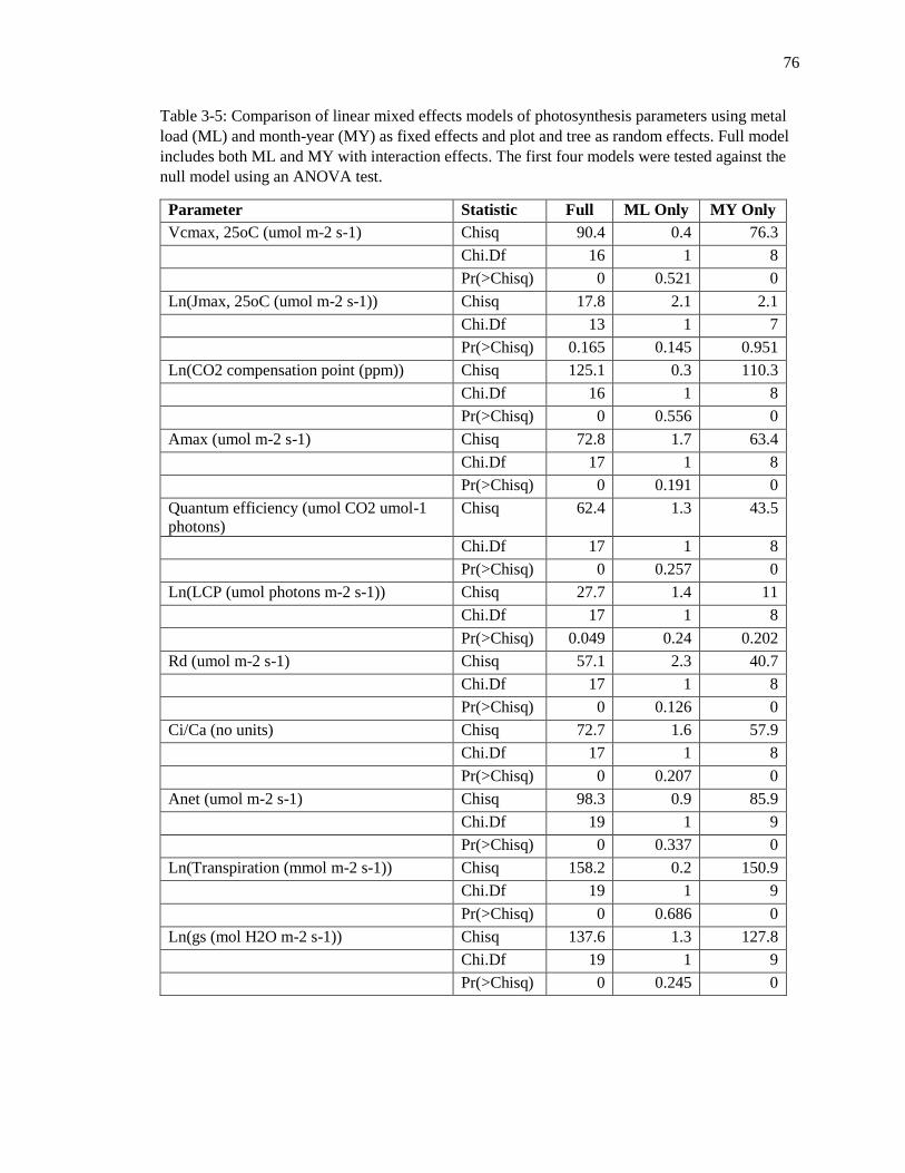
76

Table 3-5: Comparison of linear mixed effects models of photosynthesis parameters using metal

load (ML) and month-year (MY) as fixed effects and plot and tree as random effects. Full model

includes both ML and MY with interaction effects. The first four models were tested against the

null model using an ANOVA test.

Parameter Statistic Full ML Only MY Only

Vcmax, 25oC (umol m-2 s-1) Chisq 90.4 0.4 76.3

Chi.Df 16 1 8

Pr(>Chisq) 0 0.521 0

Ln(Jmax, 25oC (umol m-2 s-1)) Chisq 17.8 2.1 2.1

Chi.Df 13 1 7

Pr(>Chisq) 0.165 0.145 0.951

Ln(CO2 compensation point (ppm)) Chisq 125.1 0.3 110.3

Chi.Df 16 1 8

Pr(>Chisq) 0 0.556 0

Amax (umol m-2 s-1) Chisq 72.8 1.7 63.4

Chi.Df 17 1 8

Pr(>Chisq) 0 0.191 0

Quantum efficiency (umol CO2 umol-1

photons)

Chisq 62.4 1.3 43.5

Chi.Df 17 1 8

Pr(>Chisq) 0 0.257 0

Ln(LCP (umol photons m-2 s-1)) Chisq 27.7 1.4 11

Chi.Df 17 1 8

Pr(>Chisq) 0.049 0.24 0.202

Rd (umol m-2 s-1) Chisq 57.1 2.3 40.7

Chi.Df 17 1 8

Pr(>Chisq) 0 0.126 0

Ci/Ca (no units) Chisq 72.7 1.6 57.9

Chi.Df 17 1 8

Pr(>Chisq) 0 0.207 0

Anet (umol m-2 s-1) Chisq 98.3 0.9 85.9

Chi.Df 19 1 9

Pr(>Chisq) 0 0.337 0

Ln(Transpiration (mmol m-2 s-1)) Chisq 158.2 0.2 150.9

Chi.Df 19 1 9

Pr(>Chisq) 0 0.686 0

Ln(gs (mol H2O m-2 s-1)) Chisq 137.6 1.3 127.8

Chi.Df 19 1 9

Pr(>Chisq) 0 0.245 0

77

Table 3-5 (con’t)

Parameter Statistic Full ML Only MY Only

iWUE (umol CO2 mol-1 H2O) Chisq 72 0.2 53.9

Chi.Df 19 1 9

Pr(>Chisq) 0 0.686 0

LMA Chisq 37.6 7 16.6

Chi.Df 9 1 4

Pr(>Chisq) 0 0.008 0.002

78

Table 3-6: Variance of random effects variables used in the linear mixed effects full interactive

model for each photosynthetic parameter.

Variance

Parameter Tree Plot Residual

Vcmax at 25oC 17 0 146

Ln(Jmax at 25oC) 0 0 0.03

Ln(CO2comp) 0.004 0 0.04

Amax 1 0 9.7

φ 2.00E-06 5.00E-06 0.0001

Ln(LCP) 0 0 0.14

Rd 0.008 0 0.076

Ci/Ca 0.002 0 0.008

Photo 1.1 0 9.7

Ln(Trmmol) 0.05 0 0.38

Ln(Cond) 0.07 0 0.44

iWUE 106 0 644

79

TA

BL

E 3

-7:

Lin

ear

mix

ed e

ffec

ts m

od

el r

egre

ssio

n c

oef

fici

ents

for

full

inte

ract

ion m

odel

of

the

effe

cts

of

met

al l

oad

and

mea

sure

men

t m

on

th a

nd

yea

r on p

hoto

syn

thes

is p

aram

eter

s. S

tan

dar

d e

rrors

show

n i

n p

aren

thes

es.

Coef

fici

ents

wer

e in

cluded

in t

he

mo

del

if

thei

r 9

5%

co

nfi

den

ce i

nte

rval

did

not

incl

ude

zero

. C

oef

fici

ents

in

ita

lics

had

confi

den

ce i

nte

rval

s w

hic

h i

ncl

uded

zer

o h

ow

ever

are

in

clu

ded

bec

ause

a r

elat

ed h

igh

er l

evel

ter

m

did

. M

onth

/yea

r gro

up

s w

ith

no

sig

nif

ican

t co

effi

cien

ts w

ere

excl

uded

fro

m t

able

.

Par

am.

(In

t.)

HM

L

Jun

.

20

14

Jul.

20

14

Au

g.

20

14

Sep

.

20

14

May

.

20

15

Jun

.

20

15

Jul.

20

15

Au

g.

20

15

Sep

.

20

15

HM

L

Jul.

20

14

HM

L

Au

g.

20

14

HM

L

Sep

.

20

14

HM

L

May

20

15

HM

L

Jun

.

20

15

HM

L

Jul.

20

15

Vcm

ax

51

.8

(4)

8.9

(5.7

)

12

.3

(5.4

)

-8.1

(5.5

)

21

.6

(6.4

)

-23

.9

(8.2

)

-26

.5

(6)

-19

.9

(7.6

)

-12

.6

(7.7

)

-19

.1

(8.4

)

Ln

(Jm

ax)

4.5

5

(0.0

8)

0.2

3

(0.1

)

0.2

5

(0.1

1)

0.2

9

(0.1

3)

0.1

4

(0.1

2)

0.1

4

(0.1

1)

NA

-0.5

(0.1

4)

-0.3

9

(0.1

6)

NA

-0.3

2

(0.1

5)

-0.3

2

(0.1

4)

Ln

(Γco

mp)

4

(0.0

6)

0.2

1

(0.0

9)

0.2

1

(0.0

9)

0.3

1

(0.1

)

0.5

7

(0.0

9)

0.9

1

(0.1

3)

0.5

2

(0.1

)

Am

ax

8.4

(1

)

-3.5

(1.5

)

-3.8

(1.4

)

-6.6

(1.9

)

-4.3

(1.5

)

φ

0.0

62

(0.0

04

)

0.0

09

(0.0

05

)

0.0

07

(0.0

05

)

0.0

16

(0.0

05

)

0.0

1

(0.0

05

)

-0.0

01

(0.0

05

)

-0.0

23

(0.0

06

)

-0.0

18

(0.0

06

)

-0.0

19

(0.0

06

)

-0.0

14

(0.0

06

)

Ln

(Ico

mp)

2.9

6

(0.1

2)

-0.2

2

(0.1

7)

-0.3

5

(0.1

7)

-0.5

7

(0.1

7)

0.5

7

(0.2

4)

Rdar

k

1.1

6

(0.0

9)

-0.4

1

(0.1

2)

-0.5

8

(0.1

7)

-0.3

7

(0.1

3)

Ci/C

a

0.6

8

(0.0

3)

-0.0

8

(0.0

4)

-0.1

4

(0.0

4)

-0.2

1

(0.0

4)

-0.1

6

(0.0

6)

Anet

8.8

8

(1.0

4)

-3.9

1

(1.4

1)

-4

(1.4

1)

-7.1

2

(1.4

5)

-4.3

6

(1.4

1)

-4.2

9

(1.4

2)

Ln

(E)

0.4

1

(0.2

1)

-0.6

8

(0.2

8)

-2.4

9

(0.3

)

-0.9

8

(0.2

8)

-0.9

3

(0.2

8)

Ln

(gs)

-2

.13

(0.2

2)

-1.0

3

(0.3

)

-1.1

7

(0.3

)

-2.4

6

(0.3

3)

-1.1

2

(0.3

)

-0.8

9

(0.3

)

iWU

E

68

.6

(8.6

)

5.1

(12

.2)

36

.3

(11

.5)

54

.1

(11

.5)

25

.4

(11

.5)

67

.5

(13

.4)

-41

.4

(18

.1)

80

Table 3-8: Monthly mean temperature and total precipitation at Jersey City in 2014 and 2015 with

statewide monthly averages for comparison.

Mean Temperature (oC) Total Precipitation (cm)

Month 2014 2015 State

Average

2014 2015 State

Average

May 17 18 16 9.9 3.4 9.3

Jun 21 21 21 11.4 15.9 9.7

Jul 23 25 24 17.4 4.7 11.4

Aug 22 25 23 5.4 4.3 11.8

Sep 20 22 19 3.6 6.0 9.6

Oct 16 15 13 3.8 5.5 9.1

81

Tab

le 3

-9:

Mo

del

par

amet

ers

for

linea

r an

d p

oly

nom

ial

regre

ssio

n o

f w

eath

er v

aria

ble

s an

d p

ho

tosy

nth

etic

par

amet

ers.

Note

th

at o

nly

reg

ress

ions

wit

h s

ignif

ican

t x

or

x2 c

oef

fici

ents

(p

< 0

.05)

are

incl

uded

. S

qrt

= s

quar

e ro

ot

tran

sform

atio

n,

rcp =

rec

ipro

cal

tran

sform

atio

n,

se =

sta

ndar

d e

rror

Pa

ram

eter

W

eath

er

Inte

rcep

t (s

e)

Inte

rcep

t

p-v

alu

e x (

se)

x

p-v

alu

e x

2 (

se)

x2

p-v

alu

e A

dj.

r2

rcp

(Γco

mp (

pp

m))

D

aily

Mea

n T

emp

(oC

) 0

.02

1 (

0.0

02)

0

-0.0

00

2 (

0)

0

0.0

5

R

efer

ence

ET

(m

m/d

ay)

0.0

18 (

0.0

01)

0

-0.0

01

1

(0.0

00

4)

0.0

1

0.0

001

(0

) 0

.01

0.0

3

P

reci

p (

cm,

pre

v 2

4 h

r)

0.0

15 (

0.0

004

) 0

0

.00

2 (

0.0

01)

0.0

4

0.0

2

P

reci

p (

cm,

pre

v 7

2 h

r)

0.0

150

4

(0.0

00

42)

0

0.0

02 (

0.0

01)

0.0

3

-0.0

00

5

(0.0

00

2)

0.0

1

0.0

3

sqrt

(Am

ax (

μm

ol

m-2

s-1

))

Pre

cip

(cm

, p

rev 2

4 h

r)

2.4

(0

.07)

0

3.1

(0

.9)

0

-2.0

(0

.7)

0

0.0

6

D

aily

Mea

n T

emp

(oC

) 0

.53

(1

.1)

0.6

2

0.2

5 (

0.1

1)

0.0

2

-0.0

07

(0.0

03

) 0

.01

0.0

7

sqrt

(Anet (

μm

ol

m-2

s-1

))

Pre

cip

(cm

, p

rev 2

4 h

r)

2.4

(0

.07)

0

3.2

(0

.9)

0

-2.0

(0

.7)

0

0.0

6

D

aily

Mea

n T

emp

(oC

) 1

.3 (

1.1

) 0

.23

0.1

7 (

0.1

) 0

.1

-0.0

05

(0.0

02

) 0

.04

0.0

4

R

efer

ence

ET

(m

m/d

ay)

2.8

(0

.15)

0

-0.0

6 (

0.0

2)

0.0

2

0.0

2

sqrt

(Rd (

μm

ol

m-2

s-1

))

Dai

ly M

ean T

emp

(oC

) 0

.22

(0

.22

) 0

.33

0.0

9 (

0.0

2)

0

-0.0

02

3

(0.0

00

5)

0

0.1

2

P

reci

p (

cm,

pre

v 7

2 h

r)

0.9

3 (

0.0

2)

0

0.0

3 (

0.0

1)

0.0

1

0.0

4

R

efer

ence

ET

(m

m/d

ay)

0.9

7 (

0.0

5)

0

-0.0

3 (

0.0

2)

0.1

3

0.0

03 (

0.0

02)

0.0

5

0.0

2

sqrt

(E (

mm

ol

m-2

s-1

))

Dai

ly M

ean T

emp

(oC

) 0

.25

(0

.56

) 0

.66

0.1

1 (

0.0

6)

0.0

5

-0.0

03

(0.0

01

)

0.0

2

0.0

3

P

reci

p (

cm,

pre

v 2

4 h

r)

1.1

(0

.04)

0

1.4

(0

.5)

0

-0.8

7 (

0.3

5)

0.0

1

0.0

5

P

reci

p (

cm,

pre

v 7

2 h

r)

1.1

(0

.04)

0

0.2

2 (

0.1

0)

0.0

4

-0.0

4 (

0.0

2)

0.0

5

0.0

1

R

efer

ence

ET

(m

m/d

ay)

1.3

(0.0

8)

0

-0.0

3 (

0.0

1)

0.0

2

0.0

3

Vcm

ax (

μm

ol

m-2

s-1

) D

aily

Mea

n T

emp

(oC

) 4

.3 (

21

) 0

.84

5.4

(2

.0)

0.0

1

-0.1

4 (

0.0

5)

0.0

1

0.0

4

82

Table 3-10: Linear regression coefficients, standard error (in parentheses), and p-values (p < 0.05)

for A-Ci curve parameters using leaf temperature (Tleaf, oC) and metal load (ML) as predictors.

Leaf temperature data was centered to 30oC prior to regression. LML = low metal load, HML =

high metal load.

Paramete

r

Intercept

(LML)

p Tleaf p HML p Tleaf x

ML

p Adj.

r2

Vcmax 128.28

(7.43)

0 15.11

(2.96)

0 -14.7

(10.27)

0.16 -5.8

(3.92)

0.15 0.55

Jmax 145.05

(4.95)

0 5.59

(1.97)

0.01 -22.81

(6.83)

0 -1.99

(2.61)

0.45 0.37

Γcomp 63.11

(2.3)

0 2.73

(0.92)

0.01 -1.49

(3.17)

0.64 1.95

(1.21)

0.12 0.58

Anet 13.46

(0.87)

0 -0.26

(0.35)

0.45 -2 (1.2) 0.11 -0.55

(0.46)

0.24 0.23

Ln(gs) -1.95

(0.12)

0 -0.1

(0.05)

0.04 -0.24

(0.16)

0.16 -0.01

(0.06)

0.82 0.31

Ci 211.17

(8.92)

0 -11.43

(3.55)

0 -7.77

(12.32)

0.53 1.74

(4.7)

0.72 0.39

Ln(E) 0.76

(0.12)

0 -0.07

(0.05)

0.16 -0.19

(0.17)

0.28 0.02

(0.07)

0.78 0.08

Ci/Ca 0.71

(0.02)

0 -0.01

(0.01)

0.08 -0.02

(0.02)

0.29 0 (0.01) 0.65 0.13

83

Tab

le 3

-11:

Mea

ns

and

sta

nd

dev

iati

on

(in

par

enth

eses

) of

physi

co-c

hem

ical

soil

pro

per

ties

of

LA

I p

lots

. M

eans

wit

h t

he

sam

e le

tter

s ar

e no

t

signif

ican

tly d

iffe

ren

t acc

ord

ing t

o a

Tu

key

HS

D t

est

(p <

0.0

5)

and c

an b

e co

mpar

ed b

etw

een p

lots

an

d b

etw

een

yea

rs.

Plo

t p

H

Co

nd

uct

ivit

y

(mS

s-1

)

San

d (

%)

Sil

t (%

) C

lay

(%

)

L1

5.4

5 (

0.2

9)b

0.1

1 (

0.0

1)a

78.2

5 (

5.8

)a

19.7

5 (

5.9

7)a

1

.8 (

2)b

L2

6.0

9 (

0.3

)a

0.0

9 (

0.0

2)a

80.3

3 (

0.5

8)a

14.3

3 (

0.5

8)a

b

5 (

1)a

H2

5

.37

(0

.13

)b

0.0

9 (

0.0

1)a

81.7

5 (

3.4

)a

15 (

2.5

8)a

b

3.2

5 (

1.2

6)a

b

H3

5

.43

(0

.27

)b

0.0

8 (

0.0

1)a

85.5

(7.0

5)a

10.2

5 (

5.6

2)b

4

(1

.15)a

b

Tab

le 3

-12:

Mea

ns

and

sta

nd

dev

iati

on

(in

par

enth

eses

) M

elic

h-3

extr

acta

ble

mac

ronutr

ients

as

wel

l as

to

tal

nit

rogen

(T

N)

and

to

tal

carb

on

(T

C)

in

soil

s of

LA

I p

lots

. T

KN

= t

ota

l K

jeld

ahl

nit

rogen

. M

eans

wit

h t

he

sam

e le

tter

s ar

e not

signif

ican

tly d

iffe

ren

t ac

cord

ing t

o a

Tu

key

HS

D t

est

(p <

0.0

5)

and c

an b

e co

mp

ared

bet

wee

n p

lots

and b

etw

een y

ears

.

Plo

t T

KN

%

P (

pp

m)

K (

pp

m)

Mg

(p

pm

) C

a (

pp

m)

TN

(%

) T

C (

%)

L1

0.2

5 (

0.1

)a

79

.88

(68.9

1)a

57.8

8 (

13.6

5)a

93.7

5 (

37.4

4)b

467 (

417

)a

0.3

1 (

0.2

7)b

1

1.6

5 (

8.2

5)b

L2

0.2

3 (

0.0

6)a

6

.67

(1

.15)b

48.5

(9.6

6)a

77.6

7 (

50.2

8)a

b

395 (

305

)a

0.4

3 (

0.1

6)a

b

22

.01

(2.0

1)a

H2

0

.3 (

0.0

3)a

8

2 (

16.7

)a

76.8

8 (

8.9

4)a

101.6

2 (

21.6

5)b

306 (

142

)a

0.5

5 (

0.3

3)a

2

4.6

1 (

7.7

7)a

H3

0

.18

(0

.1)a

5

.75

(2

.72)b

61.8

8 (

25.5

4)a

96.5

(65.6

7)b

427 (

299

)a

0.3

7 (

0.1

2)a

b

18

.4 (

4.9

6)a

Tab

le 3

-13:

Mea

ns

and

sta

nd

dev

iati

on

(in

par

enth

eses

) M

elic

h-3

extr

acta

ble

mic

ronutr

ients

as

wel

l as

soil

qu

alit

y i

nd

ex (

SQ

I) v

alu

es i

n s

oil

s o

f

LA

I plo

ts. M

eans

wit

h t

he

sam

e le

tter

s ar

e not

signif

ican

tly d

iffe

rent

acco

rdin

g t

o a

Tukey

HS

D t

est

(p <

0.0

5)

and

can

be

com

par

ed b

etw

een

plo

ts

and b

etw

een

yea

rs.

Plo

t Z

n (

pp

m)

Cu

(p

pm

) B

(p

pm

) F

e (p

pm

) M

n (

act

ivit

y

ind

ex)

L1

53

.93

(58

.55

)ab

23

.57 (

12.6

7)a

b

0.4

2 (

0.1

8)a

376.4

8 (

196.3

4)a

3

7.3

6 (

12

.6)b

c

L2

4.0

3 (

3.8

7)b

2

2.2

6 (

27.6

9)a

b

0.5

2 (

0.1

6)a

451.9

3 (

43.9

6)a

1

9.9

3 (

3.1

2)a

H2

6

.56

(2

.09

)b

5.8

6 (

0.5

9)b

0.3

3 (

0.0

5)a

579.5

(29.2

7)a

2

7.4

6 (

1.7

)ab

H3

1

10

.99

(8

1.1

)a

12

4.8

1 (

115.8

4)a

0.4

1 (

0.0

5)a

486.6

5 (

266.0

1)a

5

5.4

4 (

12

.9)c

84

Table 3-14: Linear mixed effects model regression coefficients for photosynthesis parameters

modeled by water content (θg) and metal load (ML). Standard errors shown in parentheses.

Coefficients were included in the model if their 95% confidence interval did not include zero.

Parameters with no significant water content effects were excluded from table. HML = high metal

load, LML = low metal load. Sqrt = square root transformation

Parameter LML

(intercept)

HML θg HML x θg

Vcmax (μmol CO2 m-2 s-1) 33.8 (23.8) -46.9

(26.5)

75.4 (85) 223.6 (100.9)

Amax (μmol CO2 m-2 s-1) 0 (2.4) -2.5 (3.7) 29.8 (9.2) 4.2 (15.5)

Rdark (μmol CO2 m-2 s-1) 0.59 (0.19) -0.31 (0.3) 1.67 (0.76) 0.31 (1.29)

Anet (μmol CO2 m-2 s-1) 1.87 (1.36) 20.74 (7.02)

Sqrt(E [mmol H2O m-2 s-1]) 0.41 (0.16) 2.8 (0.82)

Sqrt(gs [mol H2O m-2 s-1]) 0.14 (0.05) 0.61 (0.24)

85

FIGURES Figure 3-1: Photosynthesis parameter mean values for each metal load and each measurement

month. Line length represents one standard deviation about the mean. Note data from light and A-

Ci curves measured in Plot L1 in July 2015 were excluded from the calculation of the mean for

this month since measurements were made prior to a heat wave. HML = high metal load, LML =

low metal load.

86

Figure 3-1 (con’t)

87

Figure 3-1 (con’t)

88

Figure 3-1 (con’t)

89

Figure 3-1 (con’t)

90

Figure 3-1 (con’t)

91

Figure 3-1 (con’t)

92

Figure 3-2: Box and whisker plots for each photosynthesis parameter split by metal load. Gray

circles represent individual measurements. LML = low metal load. HML = high metal load.

93

Figure 3-2 (con’t)

94

Figure 3-3: 2014 maximum and minimum daily temperatures and daily total precipitation. Data

from New Jersey Weather & Climate Network (2016)

95

Figure 3-4: 2015 maximum and minimum daily temperatures and daily total precipitation. Data

from New Jersey Weather & Climate Network (2016)

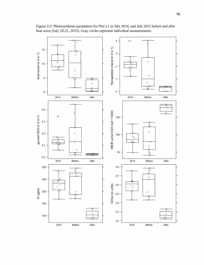
96

Figure 3-5: Photosynthesis parameters for Plot L1 in July 2014, and July 2015 before and after

heat wave (July 20-21, 2015). Gray circles represent individual measurements.

97

Figure 3-6: Mean net photosynthetic assimilation (Anet), stomatal conductance (gs), intrinsic water

use efficiency (iWUE), and transpiration (E) of low metal load (LML, closed circle) and high

metal load (HML, open circle) trees in July through September. July measurements shown here

were all made after the heat wave. Error bars represent one standard deviation.

98

Figure 3-7: Stomatal conductance (gs) versus Ci/Ca with an exponential rise to maximum function

(Singh, et al 2011) for all data (black line) as well as high metal load (HML, red) and low metal

load (LML, blue) measurements. Filled circles are measurements made in July 2015 after the heat

wave while open circles are all other measurements. Curve was fitted using data where gs > 0.01

mol H2O m-2 s-1 (based on minimum Ci/Ca) for low metal load (LML), high metal load (HML),

and combined data. The formula provided is based on combined data.

99

Figure 3-8: Linear and 2nd order polynomial regressions of weather variables and photosynthesis

parameters. Note only pairs of variables with significant x or x2 coefficients are shown.

100

Figure 3-8 (con’t)

101

Figure 3-9: Response of A-Ci parameters to leaf temperature (oC) based from trees in low metal

load (LML) and high metal load (HML) plots.

102

Figure 3-10: Response of photosynthesis parameters to gravimetric soil water content. TP-0041

(L1) and TP-0048 (L2) are low metal load plots. TP-1416 (H2) and TP-0025 (H3) are high metal

load plots. Dashed line indicates linear regression through low metal load plots. Solid line is for

high metal load plots.

103

Figure 3-10 (con’t)

104

Figure 3-10 (con’t)

105

Figure 3-10 (con’t)

106

Chapter 4 - Spatial and temporal patterns of hardwood leaf area

index in trace element contaminated soils

INTRODUCTION

Leaf area index (LAI) is the total one-sided area of leaf tissue per unit ground surface

area which is a useful parameter for characterizing a variety of plant canopies, from cornfields to

forests (Bréda 2003). It can be determined for a single plant or a group. As the plant canopy

represents the primary interface between the atmosphere and the photosynthetic machinery of the

plants, its characterization is a critical component of terrestrial biosphere models (Monson and

Baldocchi 2014). In forestry, LAI can be used to assess both spatial and temporal changes in the

canopy which may reflect forest responses to changing weather patterns or differences in soil

quality (e.g. Gaydarova 2003; Strachan and McCaughey 1996).

Methods for measuring LAI fall into one of two categories: direct or indirect. Direct

methods essentially involve measuring the area of individual leaves from part or all of a plant and

scaling up those measurements as needed. Leaves may be collected as they fall off the tree using

litterfall traps or by destructively harvesting all or part of the tree. Indirect methods estimate LAI

based on the amount of light transmitted through the canopy or rely on aerial photography. Many

studies have compared the accuracy of these methods (see Breda 2003 for review). Direct

measurements are generally assumed to be more accurate at the expense of being labor intensive

and potentially destroying the plant. The accuracy of indirect methods are dependent on how

close a canopy comes to meeting assumptions used to calculate LAI and can also be sensitive to

measurement conditions such as time of day. While LAI is a valuable metric for assessing canopy

scale productivity, it has not been extensively used to assess the effects of pollution (but see Anda

et al. 2013; Evans et al. 2015; Farrag et al. 2012).

107

Increased frequency of extreme weather events is one predicted consequence of climate

change (Romero Lankao et al. 2014). Chambers et al. (2007) estimated that Hurricane Katrina

caused the mortality of or structural damage to over 320 million large trees resulting in a loss of

105 ± 10 Tg C. It is unclear how disturbances caused by extreme weather patterns may interact

with abiotic stress from soil pollution to affect forest structure and function, both in the short and

long term. LAI has been extensively used to assess storm damage to forests using both on the

ground measurements and aerial imagery. For example, Harrington et al. (1997) found that

reductions of LAI in a Hawaiian Acacia koa forest correlated with pre-hurricane LAI and canopy

height. Landscape position and forest composition were important predictors of ice damage in a

forest in the northeastern US (Millward and Kraft 2004; Stueve et al. 2007).

Using data collected from hardwood study plots in Liberty State Park from 2010 to 2016,

I tested three hypotheses: 1) total metal load will be the primary driver of hardwood canopy leaf

area index; 2) soil nutrient availability will also be an important predictor of leaf area index; and

3) after damage caused by the Hurricane Sandy storm surge, the LAI of low metal load plots will

recover to pre-hurricane values faster.

BACKGROUND

Hurricane Sandy affected the eastern seaboard of the US from October 22 to 29, 2012.

While only effectively a post-tropical cyclone when it made landfall in New Jersey, Sandy was

particularly devastating because of the coastal storm surge it caused (Blake et al. 2013). An

analysis by FEMA Modeling Task Force (2013) as well as personal accounts indicate the

majority of Liberty State Park was inundated with water from New York Harbor. Tide data from

The Battery, New York (NOAA 2013) shows the surge lasted about 6-8 hours then retreated with

the outgoing tide. The salinity of this portion of New York Harbor fluctuates on a daily basis as

the tide mixes seawater with the outflow of the Hudson River. The salinity of the surge water

108

most likely ranged between 20 and 22 ppt (NYHOPS 2012). Tide data shows this is the only

occurrence of an ocean surge at Liberty State Park between 1995 and 2015. According to a

FEMA model (FEMA Modeling Task Force 2013) out of the six plots used in this study,

Hurricane Sandy flooding was deepest in plot L2 (1.5 m) and shallowest in plot L3 (0.2 m) (Table

4-1).

METHODS

Leaf Area Index

This study focuses on four early successional northern hardwood plots in the LSP interior

which range in total metal load index (TML, see Chapter 1 for explanation) from 0.85 to 4.31

(Table 4-1). LAI measurements were made during the growing seasons of 2010-2013, 2015-2016

though the measurement dates do not line up from year to year (Figure 4-1). Within each plot, a

transect has been maintained over the course of the entire study period to ensure measurements

are made in the same place every time samples are collected. LAI was measured using a LICOR

LI-2000 (2010) and LI-2200 (2011-2016) Plant Canopy Analyzer. To minimize the effects of

light scattering by leaves, measurements were made before 8:00 am while the sun was low in the

horizon or when the sky was uniformly overcast. From 2010 to 2013, measurements were made

using a single wand to first collect an above canopy measurement in an open field followed by

five below canopy readings then a final above. In 2015 and 2016 a two wand system was

implemented by leaving one wand in an open field to take above measurements automatically at

regular intervals while a second wand was used to make below measurements. Four to five

measurements were made at the same locations within each plot and data from these points were

combined to calculate a single LAI value for each plot on a particular day. Additionally in 2015 a

single set of measurements were made in plots L1 and H3 (similar plant community composition)

109

on July 16 & 17 to provide additional LAI data to complement a set of soil data analyzed for its

nutrient composition (details in subsequent section).

Technically, the Plant Canopy Analyzer measures plant area index (PAI) since it cannot

differentiate between the effects of foliage and woody biomass on light interception, though

estimates have suggested branches account for less than 10% of light interception in the canopy

(Kucharik et al. 1998). While there are many approaches to determining LAI from PAI (see

Bréda (2003) for review), the additional data required for these calculations are not available for

the LSP LAI data set so no corrections were made. However for the purposes of this paper, the

Plant Canopy Analyzer output will be referred to as LAI to be more consistent with conventions

in the literature.

The Plant Canopy Analyzer determines LAI indirectly using a gap fraction method. The

tool measures light transmittance in an open field and under the forest canopy at five different

zenith angles then calculates the probability of non-interception at each angle, P(θ) (the fraction

of light reaching the ground). LAI is then calculated from a solution to the Beer-Lambert Law:

5

1

2 i i

i

L K W

(1)

1

ln1 obs

ij

Nij

i

jobs i

B

AK

N S

(2)

sini i iW d (3)

Where L is Leaf Area Index (LAI), K is the contact number, Bij is the below canopy transmittance

reading for zenith angle i and observation j, Aij is the above canopy transmittance reading, Si is

the path length of zenith angle i (m, a function of canopy height and zenith angle), Wi is the

weighting factor for angle i, and θ is zenith angle (LI-COR Biosciences 2013). These calculations

110

depend on two assumptions about the forest canopy. First, the foliage are very small compared to

the overall canopy and second, the foliage is randomly distributed through the canopy (Bréda

2003). To address the first assumption, the analyzer was always held sufficiently far away from

the foliage (recommended distance is at least four times the width of the nearest leaf). While

foliage is never truly randomly distributed in a canopy, the randomness assumption is more

problematic in crop and conifer canopies.

Soil nutrients

A total of 21 soil samples were collected from the six study plots in the fall of 2015 from

the top 15 cm of soil (excluding intact leaf litter). The samples were analyzed for pH, soil texture,

electrical conductivity, macro and micronutrients by the NJAES Soil Testing Lab. A separate set

of soil samples from these plots were analyzed for total carbon (TC) and total nitrogen (TN).

Details of these analyses are provided in Chapter 3.

Stand Age Estimation

Historic aerial photography used in Gallagher et al. (2011) to assess temporal trends in

guild trajectory were used to estimate the relative ages of the hardwood forest plots used in this

study. Community guild distribution maps made for 1969, 1976, 1984, 1993, 1996, 2000, 2003,

2009, and 2015 and GPS coordinates for each plot were combined in ArcMap 10 to determine the

dominant guild of each plot in a given year. For situations where the plot appeared to be close to

the boundary of two guilds, both guilds were recorded to represent the plot as in transition during

that time period.

111

Weather Data

An analysis of the relationship between meteorological variables and LAI was made

using temperature, precipitation, and relative humidity measurements from a weather station at

Liberty Science Center, Jersey City, NJ (Station #3411) from 2010 to 2016. These measurements

were used to calculate reference evapotranspiration (ETo) rates for each day following the FAO

approach based on the Penman Monteith Equation and assuming a hypothetical reference crop

with a height of 0.12 m, fixed surface resistance of 70 s m-1 and an albedo of 0.23 (Allen et al.

1998) (see Chapter 3 for full equations). To account for lag effects that may influence canopy

development, weather variables were averaged over 1 to 4 weeks prior to the LAI measurement

date.

A series of drought indices calculated for northern New Jersey by the National Climatic

Data Center (2017) were also used in the analysis. The indices included the Palmer Drought

Severity Index (PDSI, reflects the duration and intensity of long-term drought), Palmer

Hydrological Drought Index (PHDI, reflects impacts of drought on hydrological systems such as

reservoirs), Palmer Z-index (ZNDX, measures short term drought), Modified Palmer Drought

Severity Index (PMDI, based on current observations rather than historical records), and the

standardized precipitation index (SPx, reflects probability of an observed precipitation event

based on prior precipitation patterns analyzed for x months). The primary difference between the

Palmer based and the SP indices is that the Palmer index is based on a water balance approach

while the SP is purely probability based and focuses only on precipitation (Guttman 1998). To

account for the lag effects of the drought indices, the analysis tested Palmer based variable

calculated for the 1st to 4th week preceding the LAI measurement. The analysis also used SP

indices calculated for 1, 2, 3, 6, 9, 12 and 24 months preceding LAI measurement.

112

Statistical analysis

The interacting effects of plot and measurement year were assessed using a linear model

and Tukey HSD test. To better visualize changes in LAI during the summer between plots, LAI

values from 2010 and 2012 were fitted using a moving average. Only 2010 and 2012 data were

fitted with this method since they had the highest number of samples available. Differences in soil

characteristics were compared between plots using a linear model and a Tukey HSD test. Since

soil characteristic measurements were made in the Fall of 2015, these data were only compared to

LAI data measured on July 16 and 17, 2015. These July data points were selected for analysis

since they include extra measurements made in plots L1 and H3. Soil and LAI data were

compared using a linear regression for both one soil property at a time and for pairs of soil

properties. Weather and drought index parameters were compared against LAI data collected in

2010 and 2012 using a linear regression for one parameter at a time. This analysis only used the

2010 to 2012 LAI data to avoid potential confounding effects caused by Hurricane Sandy after

2012. The models reasonably fit assumptions for normality and homogeneity of variance so no

transformations were needed.

RESULTS

LAI measurements made from 2010 to 2016 only partially supported the initial

hypothesis that low metal load (LML) plots would have the higher LAI. Instead, from 2010 to

2012 the two LML plots (L2 and L3) tended to have similar LAI values to one of the high metal

load (HML) plots (H2), ranging from around 2.5 to 3.5 (Figure 4-2, Table 4-2). Both plot and

year and their interaction were significant predictors of LAI in the four study plots (F statistic =

180.5, p < 0.001, adjusted r2 = 0.82). In 2010 a maximum LAI reading of 4.4 was made in H2, the

plot with the highest metal load in the group. The second HML plot (H1) consistently had the

lowest LAI in all study years which is in line with the initial hypothesis though contrarily H2

113

tends to have the highest LAI. Seasonal phenology of H2 appears to be slightly different from the

other three plots (Figure 4-3). In 2010 H2’s peak LAI occurs later and in 2012 its LAI decreased

until June 06 and then increased while the other three plots’ LAI mainly increased in this time

period.

Most of the macro and micronutrients measured in the six study plots had greater within

plot variation than between plot variation (Tables 4-3, 4-4, 4-5). Though P was one exception

since it was significantly higher in L1 and H2 compared to the other for plots. H1, which

consistently had the lowest LAI during the entire study, notably had the lowest mean soil pH out

of all the plots based on samples collected in 2015 (Table 4-4). The Mg soil concentrations in H1

were also significantly lower than the other study plots. Though H1’s exchangeable Zn and Cu

are comparable to those in L2, L3, and H2 (Table 4-5). On the other hand, plot H2 with the

consistently highest LAI had the highest mean P, K, and Mg (Table 4-4). H2 also had the highest

mean Fe concentration, though the highest measured value in this group of soil samples was from

H3 (Table 4-4). Forest stands also differed somewhat in age. Forest type cover had appeared in

H2 by 1976 and in L2, L3 and H1 by 1993 (Figure 4-4).

While there were not significant between plot differences for K and B, these were the

only two nutrients which showed a significant relationship with LAI in the six study plots

sampled in July 2015 (Table 4-6, Figure 4-5). While the K relationship is positive, the negative

relationship with B is surprising since all of the B concentrations are considered below optimum

for plant nutrition. Though the slope of the Fe regression was not significant, it had the third

highest r2. When the effects of nutrient pairs were tested, the adjusted r2 of the K regression was

increased by sand, silt, electrical conductivity, exchangeable Cu and Fe while the B regression

adjusted r2 was increased with the addition of silt and sand (Table 4-7).

Several weather parameters were found to be predictors of LAI when between plot

differences were accounted for by the model using 2010 to 2012 data (Table 4-8). Positive

114

relationships were observed between LAI and temperatures and reference ET averaged over the

weeks preceding LAI measurement. Negative relationships were observed with the 12-month

standardized precipitation index (SP12), though it should be noted that in the 2010 to 2012

dataset the SP12 ranged from about 0 (median conditions) to 2.5 (wetter conditions). LAI

response to temperatures averaged over 7, 14, and 21 days prior, and the reference ET averaged

14 days prior was unique for H1 (Table 4-9, Figure 4-6). While LAI in L2, L3, and H2 varied

positively with these parameters, LAI in H1 was not responsive to them. Only H2 had a

significant negative relationship for the Z-index four weeks prior to the measurement date.

In the years following the Hurricane Sandy storm surge in October 2012, LAI values in

L2, L3, and H2 were significantly lower compared to previous years (Figure 4-2, Table 4-2).

However after the hurricane LAI in H1 remained effectively unchanged. Also contrary to the

initial hypothesis, one of the LML plots (L2) had the greatest decrease in LAI after 2012 to the

point where its LAI was equivalent to that of H1. As of 2016, none of the plots which had a

significant decrease in LAI had recovered to pre-Sandy LAI levels. During the Hurricane Sandy

storm surge, of the six plots L2 had the deepest floodwater while H1 had the least (Table 4-1).

During this time period L3 and H2 continued to have similar values though by 2016 L3 LAI was

greater, though the difference is not statistically significant.

Over half of the B. populifolia trees growing in L2 died between winter 2013 and winter

2016 according to a comparison of tagged trees surveyed in both years (Table 4-10). H1 had the

lowest mortality rate in this time period, followed by L3 then H2 though it should be noted that

many of the tags were missing in H2 so those trees were not included in calculations.

115

DISCUSSION

The seven year period of LAI data collected from four hardwood plots in LSP provide

ambiguous results to the initial hypothesis which suggested high metal load (HML) plots should

have the lowest LAI. These results were unexpected since NDVI analysis of aerial imagery

showed a strong relationship between hardwood productivity and TML (Gallagher et al. 2008a).

Though several authors have pointed out that NDVI may not be sensitive to higher LAI values (>

2-3) in deciduous environments (Fassnacht and Gower 1997; Gamon et al. 1995; Ludeke et al.

1991). Studies with agricultural species (maize, Brassica spp) have found exposure to TE reduces

leaf area on a per plant basis (Anda et al. 2013; Farrag et al. 2012). Stress from salinity has also

been associated with lower LAI in mangrove forests (Gutierrez et al. 2016).

The pattern of one HML plot having the highest LAI (H2) and the other HML having the

lowest (H1) corresponds to results from Dahle et al. (2014) which found H2 had the highest

standing density (stem volume per hectare) while H1 had the lowest, leaving L2 and L3 in the

middle. This correlation suggests LAI in these plots more strongly reflects the number and size of

trees in the stand rather than the size or number of leaves on a given tree, similar to Le Dantec et

al. (2000). This interpretation is reasonable since each plot has a different stand density and

consequently the contributions of LAI from entire trees (or lack thereof) overwhelms the

measurement of LAI variation that may occur within a single tree. Drivers of LAI may be species

specific with some responding more strongly to meteorological variables while others to stand

characteristics such as stand age (Bequet et al. 2012).

The majority of weather based correlations observed in LSP LAI from 2010 to 2012 were

based on temperature and reference ET, with the exception of the 12 month standardized

precipitation index (SP12). This result is surprising considering other researchers have found

parameters such as precipitation and soil water availability to be better predictors of LAI (Bequet

et al. 2012; Le Dantec et al. 2000; Fassnacht and Gower 1997). The responses to temperature may

116

be reflecting the seasonal pattern in LAI rather than a direct effect of temperature on LAI. The

negative relationship observed between LAI and SP12 is probably the result of the limited range

of SP12 values in the study period – about 0 to 2 where 0 is median precipitation and 2 is more

rainfall than average. LAI appears to be highest when annual precipitation is close to the region’s

median value. For some temperature variables, H1 had a unique response compared to the other

three plots because while the other plots had a direct relationship with LAI and temperature H1

had effectively no relationship. This appears to stem from the smaller amplitude of change in LAI

for H1 over the course of each growing season, again suggesting that temperature may be acting

as a proxy for time of the year.

The connection between LAI and stand density at LSP is further supported by the loss of

LAI following Hurricane Sandy and the high stand mortality in plots L2, L3, and H2. Contrary to

the initial hypothesis that high metal stress would exacerbate the effects of Hurricane Sandy on

LAI, three of the four plots were similarly affected while the least affected plot has a high metal

load. It is difficult to pinpoint the precise causes of tree mortality in these LSP plots following

Hurricane Sandy since the forest was subjected to both high winds and flooding with bay water

from the storm surge. Tree death in coastal freshwater swamps in the Delmarva Peninsula also

affected by a storm surge was primarily attributed to saltwater intrusion, though evidence of wind

damage was apparent as well (Middleton 2016). It is possible that the storm surge of bay water

exposed the trees to higher concentrations of salt than they are adapted for, though the low

electrical conductivity measurements made in 2015 suggest that three years later the upper

horizons of plot soils no longer had elevated salt levels. The plot which experienced the greatest

decrease in LAI following the hurricane – L2 – was located both in a low lying area, had the

deepest floodwater (Table 4-1) and also was one of the tallest stands according to Dahle et al.

(2014). The relative heights of trees in L2 may have made them more susceptible to storm

damage (Foster 1988; Harrington et al. 1997). The decrease in LAI after the hurricane appears to

117

be primarily driven by the loss of individuals within the stand rather than stress reducing leaf size

or number in individual trees.

Clearly the pattern of standing density between the four plots also does not follow TML

either, suggesting other factors may be interacting with TML to affect standing density, and by

proxy LAI. Evans et al. (2015) assessed the relationship between ectomycorrhizal fungi (EMF) in

the four LAI plots at LSP in 2012 and 2013. EMF community composition did vary by metal

load suggesting that certain EMF communities may be better adapted to metalliferous soils. In a

separate study on soil enzyme activity at LSP, the highest LAI plot (H2) also had significantly

higher enzymatic activity, even when compared to a non-polluted reference site (Hagmann et al.

2015). Plot H2 is also unique since it has been forested for the longest period of time according to

a review of historic aerial photography. Additionally because of its age, perhaps facilitative

interactions between H2’s plants and soil community may be more robust as they have had more

time to develop. It is possible that the soil microbial community in H2 is not only well adapted to

tolerate its conditions, but in the process also facilitate aboveground productivity as well. Some

soil microbes do appear to be capable of facilitating plant growth in metal contaminated soils

possibly by producing biomolecules which can sequester the metals and limit uptake (Khan

2005).

Differences in soil physical-chemical properties may also be influencing both above and

belowground productivity in these four plots. The results of the soil nutrient analyses do lend

support to the initial hypothesis that LAI would correlate with soil nutrient availability. The trees

growing in H1 (lowest LAI) may experience the greatest nutrient limitation because of it low pH

(4.74 ± 0.17) which may reduce nutrient availability in addition to its already low concentrations

of P, K, and Mg (8.17 ± 7.01, 50.33 ± 3.79, and 37.67 ± 3.75). The higher concentrations of P, K,

and Mg in H2 (82 ± 16.7, 76.88 ± 8.94, and 101.62 ± 21.65) along with the positive relationship

between K and LAI further support the argument that nutrient availability may explain

118

differences observed between plots with similar metal load. Fassnacht and Gower (1997) also

found significant relationships between LAI and pH, K and N in conifer and hardwood forests. K

is a critical plant macronutrient need by plants in large quantities for many different functions,

including respiration, transpiration, enzyme activity and root absorption (Kaufman 1989). When a

combination of lime and pine bark mulch amendments were added around the dripline of B.

populifolia trees growing in H1, an increase in pH, P, Mg and Ca or K (but not both Ca and K at

the same time) led to altered root morphology which favored foraging (Gallagher et al. 2015).

The trees growing with some nutrient limitation may be diverting more resources to foraging

rather than aboveground productivity.

Ecosystems experiencing long term abiotic stresses such as soil pollution may be less

resilient to short term disturbances (Folke et al. 2004). In a mixed conifer-deciduous forest

downwind of a Cu smelter, plots with an experimental disturbance and high soil pollution had the

lowest rates of re-colonization and lower species richness compared to a control site (Trubina

2009). The reduction of soil nutrients caused by acid deposition correlated with a decline in

canopy density of a Norway spruce forest (Jonard et al. 2012). The authors posit that while acid

deposition had decreased with time, the stresses it imposed on the forest led to a feedback cycle

where soil stress reduced aboveground productivity which then reduced nutrient cycling leading

to further losses in aboveground productivity. However microbial communities adapted to highly

polluted soils were shown to be more resilient against the addition of new stressors, including As

and salt (Azarbad et al. 2015). Continued monitoring of the LSP stands is needed to assess the

long term resilience of this already stressed ecosystem to short term climate perturbations.

Previous work comparing plant guild trajectory between high and low metal load soils at

LSP proposed that perhaps the additional abiotic stresses imposed by the high metal soils may

lead to an alternative steady state community that differs from the typical succession community

found in the region (Gallagher et al. 2011). In this young terrestrial system, the continued addition

119

of organic material as a result of plant growth may be acting as a sink, which would reduce the

pool of available soil metals. If this concept is valid, then the strength of TML as the

deterministic abiotic filter may decrease over time leading to the establishment of species with

lower soil metal tolerance. The significant disturbance to forest structure in LSP caused by

Hurricane Sandy may alter the anticipated trajectory pattern.

The creation of canopy gaps could enable new species to establish through altering light

regimes (Schumann et al. 2003) and/or nutrient cycles (Scharenbroch 2009; Thiel and Perakis

2009). Though Carlton and Bazzaz (1998) found that Betula papyrifera seedlings, a close relative

of B. populifolia, exhibited fast growth rates on artificially disturbed microsites provided they

were not completely shaded. Two years following a hurricane which caused 70% canopy loss in a

mixedwood urban forest, the majority of the site’s soil seed bank and tree seedlings were early

successional species (Burley et al. 2008), which suggests LSP’s canopy loss could favor the

development of a new generation of birch or other early successional species. At the same time,

researchers at LSP have been observing increasing numbers of Quercus rubra and Quercus

coccinea seedlings throughout the park which also suggests the possibility of a new shift in

community composition. In the long run these gaps could also lead to greater structural

heterogeneity in the forest (Lutz and Halpern 2006). A persistent challenge for land managers is

deciding when efforts should be made to maintain a community in its current form or to allow it

to change over time. Continued tracking of the long term changes in structure and function of

these LSP plots could offer insight into the causes and effects of these changes.

CONCLUSIONS

An analysis of LAI of early successional hardwood forest plots along a gradient of metal

contamination at LSP suggests the effects of soil metal stress on aboveground canopy

productivity may be complicated by additional factors such as soil nutrients, stand age, and soil

120

community interactions. Higher nutrient levels may have some ameliorating effects on metal

stress however time may also be an important factor enabling facilitative interactions to develop.

A comparison of LAI before and after the 2012 Hurricane Sandy storm surge demonstrated the

significant reductions in canopy at the site resulting from the death of trees within three of the

four plots. As of 2016, no differences in canopy recovery have been observed between plots. It

remains to be seen how this disturbance will influence the long term structure and functions of

this forest.

121

TABLES

Table 4-1: Total metal load (TML) and estimated flood depth (m) caused by Hurricane Sandy

Storm Surge in study plots at LSP. Flood depth based on FEMA Modeling Task Force (2013)

Plot TML Flood Depth (m)

L1 0.85 1

L2 1.56 1.5

L3 1.64 0.1

H1 3.08 0.2

H2 3.56 1.2

H3 4.31 1.3

Table 4-2: Mean leaf area index (LAI) for each LAI study plot from 2010 to 2016. Standard

deviation shown in parentheses. Means with the same letters are not significantly different

according to a Tukey HSD test (p < 0.05) and can be compared between plots and between years.

Year L2 L3 H1 H2

2010 2.95 (0.19) bc 2.95 (0.23) bc 1.73 (0.29) ijk 3.44 (0.33) a

2011 3.01 (0.24) abc 2.84 (0.23) bcd 1.78 (0.39) hijk 3.16 (0.31) ab

2012 2.84 (0.36) bcd 2.69 (0.29) cde 1.68 (0.23) ijk 3.17 (0.26) ab

2013 2.06 (0.24) ghi 2.25 (0.26) fgh 1.59 (0.26) ijk 2.57 (0.27) cdef

2015 1.59 (0.16) ijk 2.42 (0.14) defg 1.45 (0.21) jk 2.6 (0.36) cdef

2016 1.38 (0.13) k 2.3 (0.11) efg 1.48 (0.15) jk 1.93 (0.23) ghij

122

Tab

le 4

-3:

Mea

ns

and

sta

nd d

evia

tio

n (

in p

aren

thes

es)

of

physi

co-c

hem

ical

soil

pro

per

ties

of

LA

I p

lots

. M

eans

wit

h t

he

sam

e le

tter

s ar

e no

t

sign

ific

antl

y d

iffe

ren

t ac

cord

ing t

o a

Tukey

HS

D t

est

(p <

0.0

5)

and c

an b

e co

mpar

ed b

etw

een p

lots

an

d b

etw

een

yea

rs.

Plo

t p

H

Con

du

ctiv

ity

(mS

s-1

)

San

d (

%)

Sil

t (%

) C

lay

(%

)

L1

5.4

5 (

0.2

9)b

0.1

1 (

0.0

1)a

78.2

5 (

5.8

)a

19.7

5 (

5.9

7)a

1

.8 (

2)b

L2

6.0

9 (

0.3

)a

0.0

9 (

0.0

2)a

80.3

3 (

0.5

8)a

14.3

3 (

0.5

8)a

b

5 (

1)a

L3

5.0

5 (

0.1

9)b

c 0.1

(0.0

4)a

79 (

0)a

16.3

3 (

0.5

8)a

b

4.6

7 (

0.5

8)a

b

H1

4.7

4 (

0.1

7)c

0.0

8 (

0.0

1)a

80.3

3 (

2.0

8)a

14.6

7 (

2.0

8)a

b

5 (

0)a

H2

5.3

7 (

0.1

3)b

0.0

9 (

0.0

1)a

81.7

5 (

3.4

)a

15 (

2.5

8)a

b

3.2

5 (

1.2

6)a

b

H3

5.4

3 (

0.2

7)b

0.0

8 (

0.0

1)a

85.5

(7.0

5)a

10.2

5 (

5.6

2)b

4

(1

.15)a

b

123

TA

BL

E 4

-4:

Mea

ns

and s

tan

d d

evia

tio

n (

in p

aren

thes

es)

Mel

ich

-3 e

xtr

acta

ble

mac

ronutr

ients

as

wel

l as

to

tal

nit

rogen

(T

N)

and

to

tal

carb

on

(TC

) in

soil

s o

f L

AI

plo

ts. T

KN

= t

ota

l K

jeld

ahl

nit

rog

en.

Mea

ns

wit

h t

he

sam

e le

tter

s ar

e not

signif

ican

tly d

iffe

ren

t ac

cord

ing t

o a

Tu

key

HS

D

test

(p <

0.0

5)

and

can

be

com

par

ed b

etw

een p

lots

and b

etw

een y

ears

.

Plo

t T

KN

%

P (

pp

m)

K (

pp

m)

Mg (

pp

m)

Ca (

pp

m)

TN

(%

) T

C (

%)

L1

0.2

5 (

0.1

)a

79.8

8 (

68.9

1)a

5

7.8

8 (

13

.65)a

9

3.7

5 (

37

.44)b

4

67 (

417)a

0.3

1 (

0.2

7)b

11.6

5 (

8.2

5)b

L2

0.2

3 (

0.0

6)a

6

.67

(1

.15)b

48.5

(9.6

6)a

77.6

7 (

50.2

8)a

b

395 (

305

)a

0.4

3 (

0.1

6)a

b

22

.01

(2.0

1)a

L3

0.2

1 (

0.0

3)a

6

.83

(3

.33)b

69.1

7 (

14.6

4)a

75.5

(21.2

3)b

169 (

48)a

0

.46

(0

.26

)ab

23

.43

(5.1

4)a

H1

0

.36

(0

.17

)a

8.1

7 (

7.0

1)b

50.3

3 (

3.7

9)a

37.6

7 (

3.7

5)a

289 (

169

)a

0.4

9 (

0.3

1)a

b

23

.81

(4.7

2)a

H2

0

.3 (

0.0

3)a

8

2 (

16.7

)a

76.8

8 (

8.9

4)a

101.6

2 (

21.6

5)b

306 (

142

)a

0.5

5 (

0.3

3)a

2

4.6

1 (

7.7

7)a

H3

0

.18

(0

.1)a

5

.75

(2

.72)b

61.8

8 (

25.5

4)a

96.5

(65.6

7)b

427 (

299

)a

0.3

7 (

0.1

2)a

b

18

.4 (

4.9

6)a

124

Tab

le 4

-5:

Mea

ns

and

sta

nd d

evia

tio

n (

in p

aren

thes

es)

Mel

ich

-3 e

xtr

acta

ble

mic

ronutr

ients

in s

oil

s of

LA

I p

lots

. M

eans

wit

h t

he

sam

e le

tter

s

are

not

signif

ican

tly d

iffe

ren

t ac

cord

ing t

o a

Tukey

HS

D t

est

(p <

0.0

5)

and c

an b

e co

mpar

ed b

etw

een

plo

ts a

nd

bet

wee

n y

ears

.

Plo

t Z

n (

pp

m)

Cu

(p

pm

) B

(p

pm

) F

e (p

pm

) M

n (

act

ivit

y

ind

ex)

L1

53.9

3 (

58.5

5)a

b

23.5

7 (

12

.67)a

b

0.4

2 (

0.1

8)a

376.4

8 (

196.3

4)a

37.3

6 (

12.6

)bc

L2

4.0

3 (

3.8

7)b

2

2.2

6 (

27.6

9)a

b

0.5

2 (

0.1

6)a

451.9

3 (

43.9

6)a

1

9.9

3 (

3.1

2)a

L3

2.8

1 (

0.9

6)b

9

.45 (

1.2

9)a

b

0.4

(0.0

3)a

402.8

(78.7

7)a

3

6.6

3 (

2.3

4)b

c

H1

3

.44

(1

.49

)b

3.5

7 (

0.5

3)b

0.4

3 (

0.0

8)a

435.1

3 (

125.1

2)a

5

1.3

(8

.13

)c

H2

6

.56

(2

.09

)b

5.8

6 (

0.5

9)b

0.3

3 (

0.0

5)a

579.5

(29.2

7)a

2

7.4

6 (

1.7

)ab

H3

1

10

.99

(8

1.1

)a

12

4.8

1 (

115.8

4)a

0.4

1 (

0.0

5)a

486.6

5 (

266.0

1)a

5

5.4

4 (

12

.9)c

125

Table 4-6: Linear regression coefficients and model r2 values for leaf area index (LAI) predicted

by individual soil nutrients. Coefficient standard errors shown in parentheses. P-values are for

individual coefficients. TN = total nitrogen, TC = total carbon, and TKN = total Kjeldahl

nitrogen. All elements with the exception of TC and TN are Mehlich 3 extractable concentrations.

Parameter Intercept p-value Slope p-value r2

K (ppm) -0.42 (0.68) 0.57 0.04 (0.01) 0.02 0.8

B (ppm) 5.29 (1.1) 0.01 -7.31 (2.61) 0.05 0.66

Fe (ppm) -0.23 (1.18) 0.85 0.01 (0) 0.1 0.53

Mg (ppm) 1.14 (0.76) 0.21 0.01 (0.01) 0.21 0.36

Sand (%) -7.67 (6.8) 0.32 0.12 (0.08) 0.22 0.35

Silt (%) 3.33 (1.21) 0.05 -0.07 (0.08) 0.41 0.17

TN (%) 1.23 (1.25) 0.38 2.33 (2.84) 0.46 0.14

Conductivity (mS s-1) 3.55 (1.77) 0.11 -14.54 (19.39) 0.5 0.12

Cu (ppm) 2.11 (0.29) 0 0 (0.01) 0.52 0.11

TC (%) 1.56 (1.1) 0.23 0.03 (0.05) 0.56 0.09

Zn (ppm) 2.14 (0.3) 0 0 (0.01) 0.62 0.07

TKN (ppm) 2.72 (1.02) 0.06 -1.92 (3.92) 0.65 0.06

Ca (ppm) 2.66 (0.84) 0.03 0 (0) 0.63 0.06

P (ppm) 2.13 (0.32) 0 0 (0.01) 0.66 0.05

pH 3.03 (3.14) 0.39 -0.15 (0.58) 0.81 0.02

Clay (%) 2.48 (0.87) 0.05 -0.06 (0.21) 0.78 0.02

Mn (activity index) 2.09 (0.79) 0.06 0 (0.02) 0.85 0.01

126

Tab

le 4

-7:

Lin

ear

regre

ssio

n c

oef

fici

ents

and m

odel

adju

sted

r2 v

alues

for

leaf

are

a in

dex

(L

AI)

pre

dic

ted

by p

airs

of

soil

nu

trie

nts

. C

oef

fici

ent

stan

dar

d e

rro

rs s

ho

wn i

n p

aren

thes

es. A

ll e

lem

ents

wit

h t

he

exce

pti

on o

f T

C a

nd T

N a

re M

ehli

ch 3

extr

acta

ble

con

centr

atio

ns.

Nu

trie

nt

1

Nu

trie

nt

2

Co

rrel

ati

on

coef

fici

ent

Mod

el p

-

valu

e

Inte

rcep

t p

-valu

e N

utr

ien

t

1 S

lop

e

p-

va

lue

Nu

trie

nt

2 S

lop

e

p-v

alu

e A

dj.

r2

K (

ppm

) S

and

(%

) 0.1

7

0.0

002

-7.8

2

(0.5

5)

0

0.0

4

(0.0

02)

0

0.0

9

(0.0

07)

0.0

01

0.9

9

K (

ppm

) S

ilt

(%)

0.0

2

0.0

01

0.6

9

(0.2

5)

0.0

7

0.0

44

(0.0

03)

0.0

01

-0.0

8

(0.0

11)

0.0

06

0.9

8

K (

ppm

) C

on

du

ctiv

ity

(mS

s-1

)

0.0

6

0.0

07

1.0

3

(0.5

2)

0.1

4

0.0

45

(0.0

05)

0.0

04

-16

.92

(4.5

85)

0.0

34

0.9

4

K (

ppm

) C

u (

pp

m)

-0.0

3

0.0

2

-0.5

8

(0.4

9)

0.3

2

0.0

44

(0.0

08)

0.0

11

0 (

0.0

02)

0.1

13

0.8

7

K (

ppm

) F

e (p

pm

) 0.5

3

0.0

4

-1.0

7

(0.7

2)

0.2

3

0.0

35

(0.0

11)

0.0

54

0 (

0.0

02)

0.2

19

0.8

1

B (

ppm

) S

ilt

(%)

-0.0

4

0.0

5

6.5

5

(0.9

9)

0.0

1

-7.4

83

(1.8

88)

0.0

29

-0.0

8

(0.0

37)

0.1

2

0.7

8

K (

ppm

) Z

n (

pp

m)

0

0.0

5

-0.5

1

(0.6

5)

0.4

9

0.0

44

(0.0

1)

0.0

25

0 (

0.0

03)

0.3

15

0.7

7

B (

ppm

) S

and

(%

) -0

.19

0.0

5

-2.6

2

(3.9

6)

0.5

6

-6.5

4

(1.9

83)

0.0

46

0.0

9

(0.0

46)

0.1

34

0.7

6

127

Tab

le 4

-8:

Lin

ear

regre

ssio

n c

oef

fici

ents

and m

odel

adju

sted

r2 v

alues

for

leaf

are

a in

dex

(L

AI)

mea

sure

d f

rom

20

10

to

20

12

pre

dic

ted

by a

ir

tem

per

ature

s an

d r

efer

ence

evap

otr

ansp

irat

ion (

ET

o)

aver

age

over

per

iods

of

1 t

o 4

wee

ks

as w

ell

as t

he

12

-mo

nth

Sta

ndar

diz

ed P

reci

pit

atio

n

Index

. T

able

only

sh

ow

s m

od

el p

aram

eter

s w

ith s

ignif

ican

t co

effi

cien

ts.

Coef

fici

ent

stan

dar

d e

rro

rs a

re s

ho

wn

in

par

enth

eses

.

Vari

ab

le

Mo

del

p

Ad

j. r

2

Inte

rcep

t S

lop

e P

lot

H1

Plo

t H

2

Mea

n t

emp.

1 w

eek (

oC

) <

0.0

01

0.8

3

1.8

5 (

0.2

8)

0.0

5 (

0.0

1)

0.7

7 (

0.3

9)

Mea

n t

emp

. 2

wee

k (

oC

) <

0.0

01

0.8

3

1.9

4 (

0.2

7)

0.0

4 (

0.0

1)

0

.89

(0

.38

)

Mea

n t

emp

. 3

wee

k (

oC

) <

0.0

01

0.8

2

2.0

3 (

0.2

6)

0.0

4 (

0.0

1)

0

.8 (

0.3

7)

Mea

n t

emp

. 4

wee

k (

oC

) <

0.0

01

0.8

2

2.1

2 (

0.2

6)

0.0

4 (

0.0

1)

0

.78

(0

.36

)

Mea

n E

To 1

Wee

k (

mm

) <

0.0

01

0.8

1

2.4

6 (

0.2

1)

0.0

9 (

0.0

4)

-0.7

6 (

0.2

9)

Mea

n E

To 2

Wee

k (

mm

) <

0.0

01

0.8

1

2.0

8 (

0.3

) 0.1

6 (

0.0

6)

Mea

n E

To 3

Wee

k (

mm

) <

0.0

01

0.8

1

1.9

5 (

0.3

4)

0.1

8 (

0.0

6)

Mea

n E

To 4

Wee

k (

mm

) <

0.0

01

0.8

2

1.8

6 (

0.3

8)

0.2

(0.0

7)

SP

12

< 0

.00

1

0.8

2

3.1

2 (

0.0

9)

-0.1

8 (

0.0

7)

-1.3

3 (

0.1

3)

0.3

5 (

0.1

4)

128

Tab

le 4

-9:

Lin

ear

regre

ssio

n c

oef

fici

ents

and m

odel

adju

sted

r2 v

alues

for

leaf

are

a in

dex

(L

AI)

pre

dic

ted

by t

emp

erat

ure

an

d r

efer

ence

evap

otr

ansp

irat

ion (

ET

o)

aver

aged

over

1 t

o 3

wee

ks

and

th

e Z

-in

dex

(Z

ND

X)

calc

ula

ted

fo

ur

wee

ks

pri

or

to m

easu

rem

ent

dat

e w

ith s

ignif

icant

inte

ract

ion

s b

etw

een

plo

t an

d w

eath

er v

aria

ble

. C

oef

fici

ent

stan

dar

d e

rrors

are

show

n i

n p

aren

thes

es. T

able

on

ly s

ho

ws

mo

del

par

amet

ers

wit

h

signif

ican

t co

effi

cien

ts.

Vari

ab

le

Mo

del

p

Ad

j. r

2

Inte

rcep

t S

lop

e P

lot

H1

Plo

t H

2

Slo

pe

x H

1

Slo

pe

x H

2

Mea

n t

emp

.

1 w

eek (

oC

)

< 0

.00

1

0.8

3

1.8

5 (

0.2

8)

0.0

5 (

0.0

1)

-0.3

8 (

0.3

9)

0.7

7 (

0.3

9)

-0.0

4 (

0.0

2)

Mea

n t

emp

.

2 w

eek (

oC

)

< 0

.00

1

0.8

3

1.9

4 (

0.2

7)

0.0

4 (

0.0

1)

-0.4

2 (

0.3

8)

0.8

9 (

0.3

8)

-0.0

3 (

0.0

2)

Mea

n t

emp

.

3 w

eek (

oC

)

< 0

.00

1

0.8

2

2.5

6 (

0.1

2)

0.0

3 (

0.0

1)

-0.8

6 (

0.1

7)

0.6

3 (

0.1

7)

-0.0

3 (

0.0

1)

Mea

n E

To 2

Wee

k

(mm

)

< 0

.00

1

0.8

1

2.0

8 (

0.3

) 0.1

6 (

0.0

6)

-0.3

6 (

0.4

2)

0.8

(0

.42

) -0

.16

(0

.08

)

ZN

DX

fo

ur

wee

ks

pri

or

< 0

.00

1

0.8

1

2.9

8 (

0.0

7)

0.0

6 (

0.0

5)

-1.1

9 (

0.0

9)

0.1

5 (

0.0

9)

-0

.23

(0

.07

)

129

Table 4-10: Stand mortality based on a comparison of tagged tree inventories in Liberty State

Park Study plots made in 2013 and 2016.

Plot Died after 2013 Alive in 2016 Total trees surveyed Percent died after 2013

L2 32 24 56 0.57

L3 22 59 81 0.27

H1 4 55 59 0.07

H2 12 16 28 0.43

130

FIGURES

Fig

ure

4-1

: L

eaf

area

in

dex

(L

AI)

mea

sure

men

t dat

es f

or

four

pri

mar

y s

tudy p

lots

fro

m 2

010 t

o 2

01

6.

Eac

h s

qu

are

indic

ates

a

mea

sure

men

t d

ate.

131

Fig

ure

4-2

: L

eaf

area

in

dex

(L

AI)

of

plo

ts T

P-4

8,

TP

-43,

TP

-14 a

nd T

P-1

416 a

t L

SP

duri

ng t

he

20

10

-20

16

gro

win

g s

easo

ns

(ex

clu

din

g 2

01

4).

Cir

cles

rep

rese

nt

mea

sure

men

t dat

es. T

P-4

8 (

L2)

and T

P-4

3 (

L3)

are

low

met

al l

oad

plo

ts w

hil

e T

P-1

4 (

H1

) an

d T

P-1

41

6 (

H2)

are

hig

h m

etal

load

plo

ts.

132

Figure 4-3: Moving averages of leaf area index (LAI) of four plots in 2010 and 2012.

133

Fig

ure

4-4

: P

lant

gu

ild

tra

ject

ori

es f

or

sele

cted

stu

dy p

lots

in L

iber

ty S

tate

Par

k b

ased

on a

n a

nal

ysi

s o

f ae

rial

ph

oto

gra

ph

y i

n G

alla

gh

er e

t al

.

(2011).

So

lid

lin

es i

ndic

ate

the

yea

rs w

hen

aer

ial

photo

gra

phs

wer

e ta

ken

. B

are

(lig

ht

yel

low

) =

bar

e so

il,

Hb

(li

gh

t gre

en)

= h

erb

/forb

e, S

h

(med

ium

gre

en)

= s

hru

b, S

NH

(d

ark g

reen

) =

succ

essi

onal

nort

her

n h

ardw

ood.

Plo

t to

tal

met

al l

oad

incr

ease

s d

ow

n t

he

char

t.

134

Fig

ure

4-5

: L

eaf

area

in

dex

(L

AI)

of

plo

ts m

easu

red o

n J

uly

16 a

nd 1

7,

2015 p

redic

ted b

y M

ehli

ch 3

ex

trac

tab

le p

ota

ssiu

m,

bo

ron

, an

d i

ron

(ppm

). M

easu

rem

ents

wer

e m

ade

in p

lots

L1, L

2,

L3, H

1,

H2,

and H

3.

Hori

zonta

l er

ror

bar

s re

pre

sen

t o

ne

stan

dar

d d

evia

tio

n a

bo

ut

the

mea

n

SQ

I (n

= 3

for

L2

, L

3, H

1 a

nd

n =

4 f

or

L1,

H2,

H3).

135

FIGURE 5-6: Selected weather parameters with significant plot x parameter interactions for leaf

area index (LAI) measured in 2010 to 2012. WeeklyTempAvg.C = temperature averaged over the

7 days preceding measurement date. BiWeeklyTempAvg.C = temperature averaged over the 14

days preceding measurement date. TriWeeklyTempMin.C = temperature minimum during the 21

days preceding measurement date. BiWeeklyEToAvg.mm = reference evapotranspiration

averaged over the 14 days preceding the measurement date. ZNDX.n.28 = Z-index value four

weeks prior to measurement date.

136

Chapter 5 - Synthesis & Conclusion

The goal of this dissertation was to begin addressing the question: What are the

mechanisms by which soil trace element contamination affects primary forest productivity? The

accurate quantification and prediction of ecosystem functions across a range of conditions is

necessary for many applications, including terrestrial biosphere modelling (e.g. Medvigy et al.

2009), natural resource management (Cox et al. 2013), and restoration ecology (Hooper et al.

2016). Yet as Rohr et al. (2016) explain, there is a fundamental challenge to connect data

collected on individual responses to environmental contaminants to the broader ecosystem

functions of greatest interest to society. The interior forest in Liberty State Park (LSP) provides a

unique opportunity to assess responses to TE contamination at multiple scales since the forest has

been established for several decades in the contaminated soil. This site allows us to study TE

effects as the ecosystem continues to develop and possibly goes through a transition phase rather

than during the establishment phase of restoration which has been the focus of other studies

(Baeten et al. 2010; Beesley et al. 2010; Dickinson 2000; Oldfield et al. 2015; Perez-de-Mora et

al. 2006).

In particular, this research focused on testing the hypothesis that higher soil TE

concentrations would reduce photosynthesis and related processes in Betula populifolia, thereby

reducing overall net primary productivity and tree growth. Dramatic differences in leaf level

photosynthesis were not observed between plots in LSP classed as having low and high metal

load soils (see Chapter 1 for total metal load description), as had been expected based on

differences in basal area growth rates observed in these groups by other studies at LSP (Dahle et

al. 2014; Renninger et al. 2012). Some significant decreases in maximum carboxylation rate and

electron transport rate of trees growing in high metal load plots were observed, however these

137

responses appear to only occur for short periods of time rather than lasting the entire growing

season.

These findings suggest that one cannot draw a straight line between individual

physiological responses to TE contamination and ecosystem level primary productivity, at least

with mature hardwood trees. Instead, TE may exert greater influence as an abiotic filter during

the establishment phase. TE may also affect multiple levels of biological organization which in

turn interact with each other and respond to other environmental conditions. To understand the

effects of TE on primary productivity based on the body of research conducted at LSP, I propose

a conceptual model which accounts for both TE effects on multiple levels of biological

organization as well as interacting effects which occur between levels in hardwood ecosystems

(Figure 5-1). This model is based on work by Fattorini and Halle (2004) and Rohr et al. (2016).

The conceptual model accounts for TE impacts on community composition through the

role of TE as an abiotic filter on species establishment (Figure 5-1 Part A). Community

composition becomes limited to those species which possess traits which enable tolerance of the

TE stress (or another condition typical of degraded soil such as nutrient deficiency) (Fattorini and

Halle 2004). Hardwood biodiversity decreased with increasing TE concentrations at Liberty State

Park (Gallagher et al. 2008b), and similarly in other sites plant distribution follows patterns of

contamination (Desjardins et al. 2014). This filtering sets the stage for future interactions and the

development of biodiversity within the site. It is well accepted that ecosystem functions generally

scale positively with biodiversity (Hooper et al. 2005). However it is unclear how the addition of

stress from soil pollution could influence that relationship.

In addition to filtering out entire species, TE contamination also acts a filter on genetic

variation within species or local populations by favoring TE tolerant phenotypes. It is possible

that the robust nature of photosynthesis rates between the low and high metal load trees at LSP

stems from the site selecting for individuals with TE tolerant physiological processes. High

138

within species variability in TE tolerance has been observed in other species commonly planted in

restoration and remediation settings, such as poplar (Gaudet et al. 2011). In order for spontaneous

revegetation projects to be successful, the regional species and genetic pool need to contain

material that is tolerant of stressful site conditions. It has been hypothesized that the original

seeds of the LSP Betula populifolia trees may have travelled from as far as the coal mining

regions of Pennsylvania. Though genetic material could have also travelled south out of the

Hudson Valley as well. If this is indeed the case, then this would imply that the revegetation of

novel anthropogenic soils may require a species pool from a large geographic region and possibly

human intervention to access adequate genetic material. A genetic comparison of B. populifolia

growing in LSP and from other populations in New Jersey, New York, and Pennsylvania could

help to address this question and provide insight into the nature of regional species pools in urban

environments.

In addition to an abiotic filter, biotic interactions undoubtedly have an effect on

community composition through facilitative, competitive, and predator-prey interactions (Figure

5-1 Part B) (Fattorini and Halle 2004). More research is needed to understand how TE

contamination may alter the magnitude and relative importance of these different types of

interactions. Krumins et al. (2015) have suggested that in stressful environments, facilitation may

play an important role in the development of communities. Research on leaf area index at LSP by

Evans et al. (2015) suggests plant-mycorrhizal interactions may play a role in maintaining higher

primary productivity in high metal load soils. As our ability to sequence and study soil microbial

communities continues to improve, future research and modeling efforts can begin to account for

the role of microbiota on aboveground ecosystem functions in degraded habitats.

TE contamination may directly influence organism physiology and growth (Figure 5-1

Part C). The B. populifolia photosynthesis data demonstrates that this effect may be seasonal or

transient. Other photosynthesis research at LSP also suggests that these effects may be mediated

139

by other factors such as edaphic conditions or plant age (Radwanski et al. 2017; Renninger et al.

2012). While physiological responses of individual species to individual toxicants may be readily

studied in laboratory and greenhouse settings (Rohr et al. 2016), the findings from LSP suggest

that fine scale physiology may not be as important to the bigger picture of ecosystem function in

well-established forest communities.

Allometry of individuals is likely influenced by both TE stress and interactions with other

individuals (Figure 5-1 Part D). Direct exposure of roots to contaminants (Zhang et al. 2014),

carbon demands of mycorrhizal fungi (Allen et al. 2003), and increased foraging in nutrient poor

soil (Poorter et al. 2011) could all divert more carbon resources to the root zone rather than to

aboveground growth. At the same time, stand density can exert a strong influence on

aboveground resource allocation, altering tree height and diameter ratios and branch growth

(Donoso and Nyland 2006). Stand density can be influenced by many factors, including

succession or community trajectory patterns (Royo and Carson 2006). At LSP, vegetative guild

trajectory varied between low and high metal load soils and may explain current patterns of stand

density and allometry observed in study plots. If this is the case, then TE stress affects individual

growth patterns both directly and indirectly which would further complicate modeling efforts.

Other edaphic conditions and disturbance events may also affect population

characteristics and community composition (Figure 5-1 Part E). Many anthropogenic soils have

multiple characteristics which can be detrimental to plant growth in addition to pollution,

including low nutrient availability, extreme pH, and poor drainage (Morel et al. 2014). The leaf

area index data at LSP highlighted the role nutrient availability may play in influencing canopy

productivity. Major disturbances such as the Hurricane Sandy storm surge may lead to a state

change in the system. As canopy was opened following tree mortality post-storm surge, it is

possible new species may be able to gain a foothold in these canopy gaps (Muscolo et al. 2014).

This situation will provide an interesting opportunity to see if TE contamination makes

140

established communities more or less resistant to invasion following a disturbance. The TE

contamination may continue to act as a strong filter on species recruitment favoring the regrowth

of species already in the site. Alternatively if ecosystem development over the past few decades

has sufficiently influenced the availability of TE and/or mitigated other detrimental

characteristics of the soil through the addition of organic matter, perhaps new species will be able

to establish. If new species have different TE accumulation patterns or produce biomass with

different decomposition rates, these changes could alter long term TE stability.

TE contamination affects primary productivity through its effects on community

composition, individual physiology (possibly to a lesser degree), community trajectory and

population characteristics (Figure 5-1 Part F). At the same time primary productivity is also

influenced by other edaphic conditions within the site as well as the interactions of organisms

within the community. These numerous interrelationships coupled with the longevity of trees

makes developing a mechanistic understanding of TE impacts on hardwood primary productivity

challenging. Given the long-lived nature of trees, the body of research at LSP suggests or

demonstrates how the early effects of TE on community assembly (i.e. influencing species

composition and guild trajectory) may have lasting consequences on the structure and function of

the community.

Ecosystem functions may in turn influence TE concentrations and/or availability over

time through TE uptake and the addition of organic matter to the soil (Figure 5-1 Part G). The

results from the analysis of the 20 years of LSP soil data suggest the potential for plant growth

(i.e. primary productivity) and possibly decomposition to stabilize concentrations of at least some

of the TE at the site. It is unclear if this stability will mean that the TE will continue to act as an

abiotic filter on species establishment. Alternatively, while pseudo-total TE concentrations have

remained stable their availability may have increased or decreased which could then alter the

nature of the TE-based filter. Concurrently, as the soil continues to develop with the addition and

141

subsequent decomposition of organic matter along with other soil forming processes, the role of

the soil as a filter may change as well. Following up on previous biodiversity studies at the site

could offer insight into the changing role of the soil as a filter on community composition over

time.

Taken all together, this conceptual model highlights the potential for TE to influence

hardwood primary productivity through multiple mechanisms, and equally important how

primary productivity may influence the TE. In its current form, this model is derived from the

pieces of many different research projects conducted at LSP. One approach to test the accuracy

and utility of the model would be to use data from these LSP studies to parameterize it, possibly

borrowing approaches from ecotoxicological (e.g. Forbes and Calow 2013; Martin et al. 2013),

terrestrial biosphere (e.g. Medvigy et al. 2009) and/or community assembly models (e.g. Laughlin

2014) to assess how well these research pieces fit together. Fitting such model could reveal what

components of the system may have been overlooked thus far or highlight which components are

more or less important drivers of hardwood primary productivity in TE contaminated soil.

Another next step in studying the mechanisms by which TE contamination influence

primary productivity will be to generalize findings from LSP in such a way as to be both

comparable to and useful for other sites and projects. This next step could enable better prediction

capabilities for environmental resource assessments (ERA) and improved expectations and

treatment for restoration projects (Hooper et al. 2016). Trait-environment frameworks have been

proposed as one strategy for enabling comparisons across sites and ecosystems (Perring et al.

2015). Trait-environment frameworks assess the distribution of selected traits (e.g. seed size)

along an environmental gradient (e.g. soil moisture) (Pavoine et al. 2011). One could choose an

environmental characteristic (or more likely a set of them) and then find where a site fits along

that gradient in order to compare its community structure and function to other sites. Relatively

new developments in the creation of soil taxonomies for urban and anthropogenic soils could also

142

be valuable in facilitating comparisons between sites. These taxonomies provide a richer

vocabulary and framework to replace the rudimentary use of “urban” as a soil classifier. Morel et

al. (2014) propose a set of broad classifications for soils in urban, industrial, transportation, and

mining areas (collectively referred to as SUITMAs) and posit different ecosystem functions each

could support. But this SUITMA-ecosystem function framework has not been tested. One could

assess how biodiversity changes with level of anthropogenic impact using a metric such as the

amount of anthropogenic material in a soil.

At LSP in particular, there are several other important directions for future research.

Turner et al. (2003) contend a major limitation of many ecosystem service studies is their focus

on one service at a time even though in reality many ecosystem functions occur together or may

operate in opposition. The LSP hardwood studies have been essentially focused on primary

production. Future research should assess other ecosystem functions across the trace element

gradient such as nutrient cycling or habitat provisioning. Additionally as mentioned in Chapter 4,

observations have been made of a growing number of mid-successional oak trees growing in the

park. Research has started tracking the location and basal area growth of these trees including

several transects of seedling location. Since research on other hardwoods at the site has

highlighted the importance of other edaphic conditions along with metal load, additional

measurements such as macronutrient availability could be made along these oak transects to

complement TE data.

Conclusion

Trace element contaminated soils are a persistent problem and one that will continue to

grow with increasing urbanization and global development. Consequently it is important to

understand how the trace elements not only affect individual organisms but ecosystem functions

143

as a whole. Additionally, given the persistent nature of trace elements it is crucial for research to

focus on the long term fate and effects of these contaminants. Research at Liberty State Park

found that after several decades of plant community establishment, some soil trace element

concentrations appear to have remained stable for at least two decades while others have become

enriched in the C1 horizon. These finding emphasize the importance of long term monitoring for

changing conditions that could affect the fate of these elements. Measurements of photosynthetic

parameters of Betula populifolia growing at the site show that overall the photosynthetic

parameters of these trees are fairly robust along a range of increasing trace element

concentrations. When differences were observed they appear to last for a short period of time

suggesting the possibility that trace element effects may be seasonal. Six years of leaf area index

measurements demonstrated that other plot or stand specific characteristics such as nutrient

availability, soil microbial community, and age may interact with or overwhelm trace element

stress effects on canopy productivity. Taken together, these findings illustrate the complications

of assessing trace element effects in field systems and the ways multiple factors may interact to

influence primary productivity in trace element contaminated forests. They also demonstrate the

potential of such ecosystems to function in spite of severe abiotic stresses.

144

FIGURES Figure 5-1: Conceptual diagram representing the effects of trace element contamination on

primary productivity through effects at lower levels of biological organization and interactions

between levels in a hardwood ecosystem. A) Trace element contamination operates as an abiotic

filter on community composition. B) Interactions such as symbiotic relationships with

mycorrhizal fungi influence population characteristics and individual growth. C) Trace element

influence individual physiology. D) Individual growth and allometry is affected by population or

stand characteristics. E) Edaphic conditions and disturbance can influence population dynamics.

F) Primary productivity is an emergent property from all of these relationships. G) Plant growth

and addition of organic matter to sol can modify trace element concentrations and availability

over time.

145

WORKS CITED

Aalto, T., and Juurola, E. (2001). “Parametrization of a biochemical CO 2 exchange model for

birch ( Betula pendula Roth .).” Boreal Environment Research, 6(March), 53–64.

Ajmone-Marsan, F., and Biasioli, M. (2010). “Trace elements in soils of urban areas.” Water, Air,

and Soil Pollution, 213(1–4), 121–143.

Al-Tabbaa, A., Smith, S., Munck, C. De, Dixon, T., Doak, J., Garvin, S., and Raco, M. (2007).

“Climate Change, Pollutant Linkage and Brownfield Regeneration.” Sustainable Brownfield

Regeneration, T. Dixon, M. Raco, P. Catney, and D. Lerner, eds., Blackwell Publishing Ltd,

Oxford, UK.

Allen, M. F., Swenson, W., Querejeta, J. I., and Treseder, K. K. (2003). “Ecology of

Mycorrhizae: A Conceptual Framework for Complex Interactions Among Plants and

Fungi.” Annual Review of Phytopathology, 41, 271–303.

Allen, R. G., Pereira, L. S., Raes, D., and Smith, M. (1998). Crop evapotranspiration -

Guidelines for computing crop water requirements - FAO Irrigation and drainage paper 56.

Rome, Italy.

Anda, A., Illes, B., and Soos, G. (2013). “Effect of cadmium pollution of atmospheric origin on

field-grown maize in two consecutive years with diverse weather conditions.” Acta

biologica Hungarica, 64(4), 476–489.

Anderson, P., Davidson, C. M., Littlejohn, D., Ure, A. M., Garden, L. M., and Marshall, J.

(1998). “Comparison of techniques for the analysis of industrial soils by atomic

spectrometry.” International Journal of Environmental Analytical Chemistry, 71(1), 19–40.

André, O., Vollenweider, P., and Günthardt-Goerg, M. S. (2006). “Foliage response to heavy

metal contamination in Sycamore Maple (Acer pseudoplatanus L.).” For. Snow Landsc.

Res, 80(3), 275–288.

Anjum, S. A., Ashraf, U., Saleem, M. F., and Wang, L. (2016). “Chromium Toxicity Induced

Alterations in Growth, Photosynthesis, Gas Exchange Attributes and Yield Formation in

Maize.” Pakistan Journal of Agricultural Sciences, 53(4), 751–757.

Ascher, J., Ceccherini, M. T., Landi, L., Mench, M., Pietramellara, G., Nannipieri, P., and

Renella, G. (2009). “Composition, biomass and activity of microflora, and leaf yields and

foliar elemental concentrations of lettuce, after in situ stabilization of an arsenic-

contaminated soil.” Applied Soil Ecology, 41(3), 351–359.

Azarbad, H., Niklińska, M., Nikiel, K., van Straalen, N. M., and Röling, W. F. M. (2015).

“Functional and compositional responses in soil microbial communities along two metal

pollution gradients: does the level of historical pollution affect resistance against secondary

stress?” Biology and Fertility of Soils, 51(7), 879–890.

Di Baccio, D., Tognetti, R., Minnocci, A., and Sebastiani, L. (2009). “Responses of the Populus x

euramericana clone I-214 to excess zinc: Carbon assimilation, structural modifications,

metal distribution and cellular localization.” Environmental and Experimental Botany,

67(1), 153–163.

Baeten, L., Velghe, D., Vanhellemont, M., De Frenne, P., Hermy, M., and Verheyen, K. (2010).

“Early Trajectories of Spontaneous Vegetation Recovery after Intensive Agricultural Land

146

Use.” Restoration Ecology, 18(SUPPL. 2), 379–386.

Beesley, L., Moreno-Jiménez, E., Gomez-Eyles, J. L., and Moreno-Jimenez, E. (2010). “Effects

of biochar and greenwaste compost amendments on mobility, bioavailability and toxicity of

inorganic and organic contaminants in a multi-element polluted soil.” Environmental

Pollution, 158(6), 2282–7.

Bequet, R., Kint, V., Campioli, M., Vansteenkiste, D., Muys, B., and Ceulemans, R. (2012).

“Influence of stand, site and meteorological variables on the maximum leaf area index of

beech, oak and Scots pine.” European Journal of Forest Research, 131(2), 283–295.

Van Den Berge, J., Naudts, K., Janssens, I. A., Ceulemans, R., and Nijs, I. (2011). “Does the

stress tolerance of mixed grassland communities change in a future climate? A test with

heavy metal stress (zinc pollution).” Environmental Pollution, Elsevier Ltd, 159(12), 3294–

3301.

Bernacchi, C. J., Pimentel, C., and Long, S. P. (2003). “In vivo temperature response functions of

parameters required to model RuBP-limited photosynthesis.” Plant, Cell and Environment,

26(9), 1419–1430.

Bernacchi, C. J., Singsaas, E. L., Pimentel, C., Portis, a. R. J., and Long, S. P. (2001). “Improved

temperature response functions for mod- els of Rubisco-limited photosynthesis.” Plant, Cell

and Environment, 24(2), 253–260.

Blake, E. S., Kimberlain, T. B., Berg, R. J., Cangialosi, J. P., and Beven, J. L. (2013). Tropical

Cyclone Report - Hurricane Sandy (AL182012).

Blake, L., and Goulding, K. W. T. (2002). “Effects of atmospheric deposition, soil pH and

acidification on heavy metal contents in soils and vegetation of semi-natural ecosystems at

Rothamsted Experimental Station, UK.” Plant and Soil, 240(2), 235–251.

Bleeker, P. M., Assunção, A. G. L., Teiga, P. M., De Koe, T., and Verkleij, J. A. C. (2002).

“Revegetation of the acidic, As contaminated Jales mine spoil tips using a combination of

spoil amendments and tolerant grasses.” Science of the Total Environment, 300(1–3), 1–13.

Bodek, I., Lyman, W. J., Reehl, W. F., and Rosenblatt, D. H. (1988). Environmental Inorganic

Chemistry: Properties, Processes and Estimation Methods. (B. T. Walton and R. A.

Conway, eds.), Pergamon Press, New York City, NY.

Bolan, N., Kunhikrishnan, A., Thangarajan, R., Kumpiene, J., Park, J., Makino, T., Kirkham, M.

B., and Scheckel, K. (2014). “Remediation of heavy metal(loid)s contaminated soils – To

mobilize or to immobilize?” Journal of Hazardous Materials, Elsevier B.V., 266, 141–166.

Boone, R., Tardif, J., and Westwood, R. (2004). “Radial growth of oak and aspen near a coal-

fired station, Manitoba, Canada.” Tree-Ring Research, 60(1), 45–58.

Borgegard, S.-O., and Rydin, H. (1989). “Biomass, root penetration and heavy metal uptake in

birch in a soil cover over copper tailings.” Journal of Applied Ecology, 26, 585–595.

Bréda, N. J. J. (2003). “Ground-based measurements of leaf area index: A review of methods,

instruments and current controversies.” Journal of Experimental Botany, 54(392), 2403–

2417.

Brodribb, T. (1996). “Dynamics of Changing Intercellular CO2 Concentration (ci) during

Drought and Determination of Minimum Functional ci.” Plant physiology, 111(1), 179–185.

147

Brown, S., Chaney, R. L., Hallfrisch, J. G., and Xue, Q. (2000). “Effect of biosolids processing

on lead bioavailability in an urban soil.” Journal of environmental quality, 32, 100–108.

Brun, L. A., Le Corff, J., and Maillet, J. (2003). “Effects of elevated soil copper on phenology,

growth and reproduction of five ruderal plant species.” Environmental Pollution, 122(3),

361–368.

Buchter, B., Davidoff, B., Amacher, M. C., Hinz, C., Iskandar, I. K., and Selim, H. M. (1989).

“Correlation of Freundlich Kd and retention parameter with soils and elements.” Soil

Science, 148(5), 370–379.

Burley, S., Robinson, S. L., and Lundholm, J. T. (2008). “Post-hurricane vegetation recovery in

an urban forest.” Landscape and Urban Planning, 85(2), 111–122.

von Caemmerer, S. (2000). Biochemical Models of Leaf Photosynthesis. CSIRO Publishing,

Collingwood, Australia.

Cannell, M. G. R., and Thornley, J. N. M. (2000). “Modelling the Components of Plant

Respiration : Some Guiding Principles.” Annals of Botany, 85, 45–54.

Carlton, G. C., and Bazzaz, F. A. (1998). “Regeneration of three sympatric birch species on

experimental hurricane blowdown microsites.” Ecological Monographs, 68(1), 99–120.

Castro-Rodríguez, A., Carro-Pérez, M. E., Iturbe-Argüelles, R., and González-Chávez, J. L.

(2015). “Adsorption of hexavalent chromium in an industrial site contaminated with

chromium in Mexico.” Environmental Earth Sciences, 73(1), 175–183.

Cervelli, E. W., Lundholm, J. T., and Du, X. (2013). “Spontaneous urban vegetation and habitat

heterogeneity in Xi’an, China.” Landscape and Urban Planning, 120, 25–33.

Chambers, J. Q., Fisher, J. I., Zeng, H., Chapman, E. L., Baker, D. B., and Hurtt, G. C. (2007).

“Hurricane Katrina’s carbon footprint on U.S. Gulf Coast forests.” Science, 318(5853),

1107.

Chen, A., Lichstein, J. W., Osnas, J. L. D., and Pacala, S. W. (2014). “Species-independent

down-regulation of leaf photosynthesis and respiration in response to shading: Evidence

from six temperate tree species.” PLoS ONE, 9(4).

Chen, M., and Ma, L. Q. (1998). “Comparison of Four USEPA Digestion Methods for Trace

Metal Analysis Using Certified and Florida Soils.” Journal of Environment Quality, 27(6),

1294–1300.

Clemente, R., Almela, C., and Bernal, M. P. (2006). “A remediation strategy based on active

phytoremediation followed by natural attenuation in a soil contaminated by pyrite waste.”

Environmental Pollution, 143(3), 397–406.

Clemente, R., Dickinson, N. M., and Lepp, N. W. (2008). “Mobility of metals and metalloids in a

multi-element contaminated soil 20 years after cessation of the pollution source activity.”

Environmental Pollution, 155(2), 254–261.

Clements, W. H., and Kiffney, P. M. (1994). “Assessing contaminant effects at higher levels of

biological organization.” Environmental Toxicology and Chemistry, 13(3), 357–359.

Cox, L. M., Almeter, A. L., and Saterson, K. A. (2013). “Protecting our life support systems: An

inventory of U.S. federal research on ecosystem services.” Ecosystem Services, Elsevier, 5,

163–169.

148

Dahle, G. A., Gallagher, F. J., Gershensond, D., Schäfer, K. V. R., and Grabosky, J. C. (2014).

“Allometric and mass relationships of Betula populifolia in a naturally assembled urban

brownfield: implications for carbon modeling.” Urban Ecosystems, 1147–1160.

Le Dantec, V., Dufrêne, E., and Saugier, B. (2000). “Interannual and spatial variation in

maximum leaf area index of temperate deciduous stands.” Forest Ecology and Management,

134(1–3), 71–81.

Denny, H., and Wilkins, D. A. (1987). “Zinc Tolerance in Betula Spp. I. Effect of external

concentration of zinc on growth and uptake.” New Phytologist, 106(3), 517–524.

Derome, J., and Nieminen, T. (1998). “Metal and macronutrient fluxes in heavy-metal polluted

Scots pine ecosystems in SW Finland.” Environmental Pollution, 103(2–3), 219–228.

Desjardins, D., Nissim, W. G., Pitre, F. E., Naud, A., and Labrecque, M. (2014). “Distribution

patterns of spontaneous vegetation and pollution at a former decantation basin in southern

Québec, Canada.” Ecological Engineering, Elsevier B.V., 64, 385–390.

DeSousa, C. A. (2003). “Turning brownfields into green space in the City of Toronto.”

Landscape and Urban Planning, 62(May 2002), 181–198.

Dickinson, N. M. (2000). “Strategies for sustainable woodland on contaminated soils.”

Chemosphere, 41(1–2), 259–263.

Dickinson, N. M., Baker, A. J. M., Doronila, A., Laidlaw, S., and Reeves, R. D. (2009).

“Phytoremediation of Inorganics: Realism and Synergies.” International Journal of

Phytoremediation, 11(2), 97–114.

Doick, K. J., Sellers, G., Castan-Broto, V., and Silverthorne, T. (2009). “Understanding success

in the context of brownfield greening projects: The requirement for outcome evaluation in

urban greenspace success assessment.” Urban Forestry and Urban Greening, Elsevier, 8(3),

163–178.

Donoso, P. J., and Nyland, R. D. (2006). “Interference to hardwood regeneration in northeastern

North America: The effects of raspberries (Rubus spp.) following clearcutting and

shelterwood methods.” Northern Journal of Applied Forestry, 23(Farmer 1997), 288–296.

Dreyer, E., Le Roux, X., Montpied, P., Daudet, F. a, and Masson, F. (2001). “Temperature

response of leaf photosynthetic capacity in seedlings from seven temperate tree species.”

Tree physiology, 21(4), 223–232.

Duursma, R. A. (2015). “Plantecophys - An R Package for Analysing and Modelling Leaf Gas

Exchange Data.” PloS one, 10(11), e0143346.

Evans, J. M., Parker, A., Gallagher, F., and Krumins, J. A. (2015). “Plant Productivity,

Ectomycorrhizae, and Metal Contamination in Urban Brownfield Soils.” Soil Science,

180(4/5), 198–206.

Farquhar, G. D., Caemmerer, S. Von, and Berry, J. A. (1980). “A Biochemical Model of

Photosynthetic CO2 Assimilation in Leaves of C3 Species.” Planta, 90, 78–90.

Farrag, K., Senesi, N., Nigro, F., Petrozza, A., Palma, A., Shaarawi, S., and Brunetti, G. (2012).

“Growth responses of crop and weed species to heavy metals in pot and field experiments.”

Environmental Science and Pollution Research, 19(8), 3636–3644.

Fassnacht, K. S., and Gower, S. T. (1997). “Interrelationships among the edaphic and stand

149

characteristics, leaf area index, and aboveground net primary production of upland forest

ecosystems in north central Wisconsin.” Canadian Journal of Forest Research, 27(7),

1058–1067.

Fattorini, M., and Halle, S. (2004). “The Dynamic Environmental Filter Model: How Do Filtering

Effects Change in Assembling Communities after Disturbance?” Assembly Rules and

Restoration Ecology, V. M. Temperton, R. J. Hobbs, T. Nuttle, and S. Halle, eds., Island

Press, Washington, 96–114.

FEMA Modeling Task Force. (2013). Hurricane Sandy Impact Analysis – Storm Surge Products.

Feng, Y. L., Auge, H., and Ebeling, S. K. (2007). “Invasive Buddleja davidii allocates more

nitrogen to its photosynthetic machinery than five native woody species.” Oecologia,

153(3), 501–510.

Folke, C., Carpenter, S., Walker, B., Scheffer, M., Elmqvist, T., Gunderson, L., and Holling, C. S.

(2004). “Regime Shifts, Resilience, and Biodiversity in Ecosystem Management.” Annual

Review of Ecology, Evolution, and Systematics, 35, 557–581.

Forbes, V. E., and Calow, P. (2013). “Developing predictive systems models to address

complexity and relevance for ecological risk assessment.” Integrated environmental

assessment and management, 9(3), e75-80.

Foster, D. R. (1988). “Species and stand response to catastrophic wind in Central New England,

USA.” Journal of Ecology, 76, 135–151.

Fox, J., and Weisberg, S. (2011). “An R Companion to Applied Regression, Second Edition.”

Sage, Thousand Oaks, Ca.

French, C. J., Dickinson, N. M., and Putwain, P. D. (2006). “Woody biomass phytoremediation

of contaminated brownfield land.” Environmental Pollution, 141(3), 387–395.

Frouz, J., Prach, K., Pizl, V., Hanel, L., Stary, J., Tajovsky, K., Materna, J., Balik, V., Kalcik, J.,

and Rehounkova, K. (2008). “Interactions between soil development, vegetation and soil

fauna during spontaneous succession in post mining sites.” European Journal of Soil

Biology, 44(1), 109–121.

Gallagher, F. J., Caplan, J. S., Krumins, J. A., and Grabosky, J. C. (2015). “Root Growth

Responses to Soil Amendment in an Urban Brownfield.” Ecological Restoration, 33(1), 10–

13.

Gallagher, F. J., Pechmann, I., Bogden, J. D., Grabosky, J., and Weis, P. (2008a). “Soil metal

concentrations and productivity of Betula populifolia (gray birch) as measured by field

spectrometry and incremental annual growth in an abandoned urban Brownfield in New

Jersey.” Environmental Pollution, Elsevier Ltd, 156(3), 699–706.

Gallagher, F. J., Pechmann, I., Bogden, J. D., Grabosky, J., and Weis, P. (2008b). “Soil metal

concentrations and vegetative assemblage structure in an urban brownfield.” Environmental

Pollution, 153(2), 351–361.

Gallagher, F. J., Pechmann, I., Holzapfel, C., and Grabosky, J. (2011). “Altered vegetative

assemblage trajectories within an urban brownfield.” Environmental Pollution, Elsevier Ltd,

159(5), 1159–1166.

Gamon, J. A., Field, C. B., Goulden, M. L., Griffin, K. L., Hartley, A. E., Joel, G., Penuelas, J.,

and Valentini, R. (1995). “Relationships between NDVI, canopy structure, and

150

photosynthesis in three Californian vegetation types.” Ecological Applications, 5(1), 28–41.

Gandois, L., Nicolas, M., VanderHeijden, G., and Probst, A. (2010). “The importance of biomass

net uptake for a trace metal budget in a forest stand in north-eastern France.” Science of the

Total Environment, Elsevier B.V., 408(23), 5870–5877.

Gaudet, M., Pietrini, F., Beritognolo, I., Iori, V., Zacchini, M., Massacci, A., Mugnozza, G. S.,

and Sabatti, M. (2011). “Intraspecific variation of physiological and molecular response to

cadmium stress in Populus nigra L.” Tree Physiology, 31(12), 1309–1318.

Gaydarova, P. N. (2003). “Deciduous forest communities in the Black Sea coastal Strandzha

region: temporal and spatial characteristics of leaf area index and density.” Trees, 17(3),

237–243.

Gessner, M. O., and Chauvet, E. (2013). “A Case for Using Litter Breakdown To Assess

Functional Stream Integrity.” Ecological Applications, 12(2), 498–510.

Good, J. E. G., Williams, T. G., and Moss, D. (1985). “Survival and growth of selected clones of

birch and willow on restored opencast coal sites.” Journal of Applied Ecology, 22, 995–

1008.

Graves, W. R., Kroggel, M. A., Widrlechner, M. P., and others. (2002). “Photosynthesis and

shoot health of five birch and four alder taxa after drought and flooding.” Journal of

Environmental Horticulture, 20(1), 36–40.

Greger, M. (2004). “Metal Availability, Uptake, Transport and Accumulation in Plants.” Heavy

Metal Stress in Plants: From Biomolecules to Ecosystems, M. N. V Prasad, ed., Springer,

Berlin, 1–27.

Gu, M., Robbins, J. A., Rom, C. R., and Choi, H. S. (2008). “Photosynthesis of birch genotypes

(Betula L.) under varied irradiance and CO2 concentration.” HortScience, 43(2), 314–319.

Guédron, S., Duwig, C., Prado, B. L., Point, D., Flores, M. G., and Siebe, C. (2014).

“(Methyl)Mercury, Arsenic, and Lead Contamination of the World’s Largest Wastewater

Irrigation System: the Mezquital Valley (Hidalgo State—Mexico).” Water, Air, & Soil

Pollution, 225(8), 2045.

Gustafsson, J. P., and Jacks, G. (1995). “Arsenic geochemistry in forsted soil profiles as revealsed

by solid-phase studies.” Applied Geochemistry, 10, 307–315.

Gutierrez, J. C. S., Ponce-Palafox, J. T., Pineda-Jaimes, N. B., Arenas-Fuentes, V., Arredondo-

Figueroa, J. L., and Cifuentes-Lemus, J. L. (2016). “Comparison of the mangrove soil with

different levels of disturbance in tropical Agua Brava Lagoon, Mexican pacific.” Applied

Ecology and Environmental Research, 14(4), 45–57.

Guttman, N. B. (1998). “Comparing the Palmer Drought Index and the Standardized Precipitation

Index.” Journal of the American Water Resources Association, 34(1), 113–121.

Hagmann, D. F., Goodey, N. M., Mathieu, C., Evans, J., Aronson, M. F. J., Gallagher, F., and

Krumins, J. A. (2015). “Effect of metal contamination on microbial enzymatic activity in

soil.” Soil Biology and Biochemistry, Elsevier Ltd, 91, 291–297.

Harrington, R. A., Fownes, J. H., Scowcroft, P. G., and Vann, C. S. (1997). “Impact of Hurricane

Iniki on Native Hawaiian Acacia koa Forests: Damage and Two-Year Recovery.” Journal of

Tropical Ecology, 13(4), 539–558.

151

Hartley, W., Dickinson, N. M., Clemente, R., French, C., Piearce, T. G., Sparke, S., and Lepp, N.

W. (2009). “Arsenic stability and mobilization in soil at an amenity grassland overlying

chemical waste ( St . Helens , UK ).” Environmental Pollution, Elsevier Ltd, 157(3), 847–

856.

Hartley, W., Dickinson, N. M., Riby, P., and Shutes, B. (2012). “Sustainable ecological

restoration of brownfield sites through engineering or managed natural attenuation? A case

study from Northwest England.” Ecological Engineering, Elsevier B.V., 40, 70–79.

Heckathorn, S. A., Mueller, J. K., Laguidice, S., Zhu, B., Heckathorn, S. A., Mueller, J. K.,

Laguidice, S., Zhu, B. I. N., Barrett, T., and Blair, B. (2017). “Chloroplast Small Heat-

Shock Proteins Protect Photosynthesis during Heavy Metal Stress.” American Journal of

Botany, 91(9), 1312–1318.

Heinrichs, H., and Mayer, R. (1980). “The role of forest vegetation in the biogeochemical cycle

of heavy metals.” Journal of Environment Quality, 9(1), 111–118.

Hermle, S., Günthardt-Goerg, M. S., and Schulin, R. (2006). “Effects of metal-contaminated soil

on the performance of young trees growing in model ecosystems under field conditions.”

Environmental Pollution, 144(2), 703–714.

Hermle, S., Vollenweider, P., Günthardt-Goerg, M. S., McQuattie, C. J., and Matyssek, R.

(2007). “Leaf responsiveness of Populus tremula and Salix viminalis to soil contaminated

with heavy metals and acidic rainwater.” Tree physiology, 27(11), 1517–1531.

Hofer, C., Gallagher, F. J., and Holzapfel, C. (2010). “Metal accumulation and performance of

nestlings of passerine bird species at an urban brownfield site.” Environmental pollution

(Barking, Essex : 1987), Elsevier Ltd, 158(5), 1207–13.

Hooper, D. U., Chapin, F. S., Ewel, J. J., Hector, A., Inchausti, P., Lavorel, S., Lawton, J. H.,

Lodge, D. M., Loreau, M., Naeem, S., Schmid, B., Setala, H., Symstad, A. J., Vandermeer,

J., and Wardle, D. A. (2005). “Effects of biodiversity on ecosystem functioning: a consensus

of current knowledge.” Ecological Monographs, 75(1), 3–35.

Hooper, M. J., Glomb, S. J., Harper, D. D., Hoelzle, T. B., Mcintosh, L. M., and Mulligan, D. R.

(2016). “Integrated risk and recovery monitoring of ecosystem restorations on contaminated

sites.” Integrated Environmental Assessment and Management, 12(2), 284–295.

Hoshika, Y., Watanabe, M., Inada, N., Mao, Q., and Koike, T. (2013). “Photosynthetic response

of early and late leaves of white birch (Betula platyphylla var. japonica) grown under free-

air ozone exposure.” Environmental Pollution, Elsevier Ltd, 182, 242–247.

Howarth, C. J. (1990). “Heat shock proteins in sorghum and pearl millet; ethanol, sodium

arsenite, sodium malonate and the development of thermotolerance.” Journal of

Experimental Botany, 41(7), 877–883.

Huang, J. H., and Matzner, E. (2007). “Biogeochemistry of organic and inorganic arsenic species

in a forested catchment in Germany.” Environmental Science and Technology, 41(5), 1564–

1569.

Itoh, Y., Noguchi, K., Takahashi, M., Okamoto, T., and Yoshinaga, S. (2007). “Estimation of

lead sources in a Japanese cedar ecosystem using stable isotope analysis.” Applied

Geochemistry, 22(6), 1223–1228.

Jardine, P. M., Stewart, M. A., Barnett, M. O., Basta, N. T., Brooks, S. C., Fendorf, S., and

Mehlhorn, T. L. (2013). “Influence of soil geochemical and physical properties on

152

chromium(VI) sorption and bioaccessibility.” Environmental Science and Technology,

47(19), 11241–11248.

Jarvinen, P., Palme, A., Orlando Morales, L., Lannenpaa, M., Keinanen, M., Sopanen, T., and

Lascoux, M. (2004). “Phylogenetic Relationshpis of Betula Species (Betulaceae) Based on

Nuclear ADH and Chloroplast MATK Sequences.” American Journal of Botany, 91(11),

1834–1845.

Jimenez, M. D., Ruiz-Capillas, P., Mola, I., Pérez-Corona, E., Casado, M. A., and Balaguer, L.

(2013). “Soil development at the roadside: A case study of a novel ecosystem.” Land

Degradation and Development, 24(6), 564–574.

Joesting, H. M., McCarthy, B. C., and Brown, K. J. (2009). “Determining the shade tolerance of

American chestnut using morphological and physiological leaf parameters.” Forest Ecology

and Management, 257(1), 280–286.

Johnson, D., MacDonald, D., Hendershot, W., and Hale, B. (2003). “Metals in northern forest

ecosystems : Role of the vegetation in Sequenstration and Cycling, and Implications for

Ecological Risk Assessment.” Human and Ecological Risk Assessment, 9(4), 749–766.

Jonard, M., Legout, A., Nicolas, M., Dambrine, E., Nys, C., Ulrich, E., van der Perre, R., and

Ponette, Q. (2012). “Deterioration of Norway spruce vitality despite a sharp decline in acid

deposition: A long-term integrated perspective.” Global Change Biology, 18(2), 711–725.

Jones, J. B. (2012). Plant nutrition and soil fertility manual. CRC Press, Boca Raton, Florida.

Juang, K. W., Lee, D. Y., and Ellsworth, T. R. (2001). “Using rank-order geostatistics for spatial

interpolation of highly skewed data in a heavy-metal contaminated site.” Journal of

Environmental Quality, 30(3), 894–903.

Jurik, T. W., Weber, J. A., and Gates, D. M. (1988). “Effects of Temperature and Light on

Photosynthesis of Dominant Species of a Northern Hardwood Forest.” Botanical Gazette,

149(2), 203–208.

Khan, A. G. (2005). “Role of soil microbes in the rhizospheres of plants growing on trace metal

contaminated soils in phytoremediation.” Journal of Trace Elements in Medicine and

Biology, 18(4), 355–364.

Kitao, M., Koike, T., Tobita, H., and Maruyama, Y. (2005). “Elevated CO2 and limited nitrogen

nutrition can restrict excitation energy dissipation in photosystem II of Japanese white birch

(Betula platyphylla var. japonica) leaves.” Physiologia Plantarum, 125(1), 64–73.

Kitao, M., Lei, T. T., and Koike, T. (1997). “Comparison of photosynthetic responses to

manganese toxicity of deciduous broad-leaved trees in northern Japan.” Environmental

Pollution, 97(1–2), 113–118.

Köhler, I. H., Macdonald, A. J., and Schnyder, H. (2016). “Last-Century Increases in Intrinsic

Water-Use Efficiency of Grassland Communities Have Occurred over a Wide Range of

Vegetation Composition, Nutrient Inputs, and Soil pH.” Plant Physiology, 170(2), 881–890.

Koike, T., and Sakagami, Y. (1986). “Comparison of the photosynthetic responses to temperature

and light of Betula maximowicziana and Betula platyphylla var. japonica.” Canadian

Journal of Forest Research, 16(6), 1397.

Kopponen, P., Utriainen, M., Lukkari, K., Suntioinen, S., Karenlampi, L., and Karenlampi, S.

(2001). “Clonal differences in copper and zinc tolerance of birch in metal-supplemented

153

soils.” Environmental Pollution, 112, 89–97.

Krumins, J. A., Goodey, N. M., and Gallagher, F. (2015). “Plant–soil interactions in metal

contaminated soils.” Soil Biology and Biochemistry, Elsevier Ltd, 80, 224–231.

Kubiske, M. E., and Pregitzer, K. S. (1996). “Effects of elevated CO2 and light availability on the

photosynthetic light response of trees of contrasting shade tolerance.” Tree Physiology,

16(3), 351–358.

Kucharik, C. J., Norman, J. M., and Gower, S. T. (1998). “Measurements of branch area and

adjusting leaf area index indirect measurements.” Agricultural and Forest Meteorology,

91(1–2), 69–88.

Kumpiene, J., Lagerkvist, A., and Maurice, C. (2008). “Stabilization of As, Cr, Cu, Pb and Zn in

soil using amendments - A review.” Waste Management, 28(1), 215–225.

De Laender, F., De Schamphelaere, K. A. C., Vanrolleghem, P. A., and Janssen, C. R. (2008).

“Validation of an ecosystem modelling approach as a tool for ecological effect

assessments.” Chemosphere, 71(3), 529–545.

Landre, A. L., Watmough, S. a., and Dillon, P. J. (2009). “Metal Pools, Fluxes, and Budgets in an

Acidified Forested Catchment on the Precambrian Shield, Central Ontario, Canada.” Water,

Air, & Soil Pollution, 209(1–4), 209–228.

Landre, A. L., Watmough, S. A., and Dillon, P. J. (2010). “Metal pools, fluxes, and budgets in an

acidified forested catchment on the precambrian shield, central Ontario, Canada.” Water,

Air, and Soil Pollution, 209(1–4), 209–228.

Larson, C. (2014). “China Gets Serious About Its Pollutant-Laden Soil.” Science, 343(6178),

1415–1416.

Laughlin, D. C. (2014). “Applying trait-based models to achieve functional targets for theory-

driven ecological restoration.” Ecology Letters, 17(7), 771–784.

LI-COR Biosciences. (2013). LAI-2200C Plant Canopy Analyzer Instruction manual. Lincoln,

NE.

Li, J., Shoup, S., and Chen, Z. (2007). “Phylogenetic Relationships of Diploid Species of Betula (

Betulaceae ) Inferred from DNA Sequences of Nuclear Nitrate Reductase.” Systematic

Botany, 32(2), 357–365.

Li, Y.-M., Chaney, R. L., Siebielec, G., and Kerschner, B. A. (1999). “Response of four turfgrass

cultivars to limestone and biosolids-compost amendment of a zinc and cadmium

contaminated soil at Palmerton, Pennsylvania.” Journal of Environment Quality, 29(5),

1440–1447.

Li, Z., and Huang, L. (2015). “Toward a new paradigm for tailings phytostabilization - nature of

the substrates, amendment options, and anthropogenic pedogensis.” Critical Reviews in

Environmental Science and Technology, 45(8), 813–839.

Linn, J. (2013). “The effect of voluntary brownfields programs on nearby property values:

Evidence from Illinois.” Journal of Urban Economics, Elsevier Inc., 78, 1–18.

Liu, X., Song, Q., Tang, Y., Li, W., Xu, J., Wu, J., Wang, F., and Brookes, P. C. (2013). “Human

health risk assessment of heavy metals in soil-vegetable system: A multi-medium analysis.”

Science of the Total Environment, Elsevier B.V., 463–464, 530–540.

154

Lobo, F. de A., de Barros, M. P., Dalmagro, H. J., Dalmolin, Â. C., Pereira, W. E., de Souza, É.

C., Vourlitis, G. L., and Rodríguez Ortíz, C. E. (2013). “Fitting net photosynthetic light-

response curves with Microsoft Excel - a critical look at the models.” Photosynthetica,

51(3), 445–456.

Losch, R. (2004). “Plant Mitochondrial Respiration Under the Influence of Heavy Metals.” Heavy

Metal Stress in Plants: From Biomolecules to Ecosystems, M. N. V. Prasad, ed., Springer,

Berlin, 182–200.

Ludeke, M., Janecek, A., and Kohlmaier, G. (1991). “Modelling the seasonal CO2 uptake by land

vegetation using the global vegetation index.” Tellus B, 43(2), 188–196.

Lutz, J. A., and Halpern, C. B. (2006). “Tree Mortality during Early Forest Development : A

Long-Term Study of Rates , Causes , and Consequences.” Ecological Monographs, 76(2),

257–275.

Ma, Y., Prasad, M. N. V, Rajkumar, M., and Freitas, H. (2011). “Plant growth promoting

rhizobacteria and endophytes accelerate phytoremediation of metalliferous soils.”

Biotechnology Advances, 29(2), 248–258.

MacFarlane, G. R., and Burchett, M. D. (2000). “Cellular distribution of Cu, Pb and Zn in the

Grey Mangrove Avicennia marina (Forsk.). 68, 45 – 59.” Vierh. Aquat. Bot., 68, 45–59.

Maggio, A., and Joly, R. J. (1995). “Effects of mercuric chloride on the hydraulic conductivity of

tomato root systems.” Plant Physiology, 109, 331–335.

Margui, E., Queralt, I., Carvalho, M. L., and Hidalgo, M. (2007). “Assessment of metal

availability to vegetation (Betula pendula) in Pb-Zn ore concentrate residues with different

features.” Environmental Pollution, 145(1), 179–184.

Martin, B. T., Jager, T., Nisbet, R. M., Preuss, T. G., Hammers-Wirtz, M., and Grimm, V. (2013).

“Extrapolating ecotoxicological effects from individuals to populations: A generic approach

based on Dynamic Energy Budget theory and individual-based modeling.” Ecotoxicology,

22(3), 574–583.

McBride, M., Sauve, S., and Hendershot, W. (1997). “Solubility control of Cu, Zn, Cd and Pb in

contaminated soils.” European Journal of Soil Science, 48(2), 337–346.

McComb, J. Q., Rogers, C., Han, F. X., and Tchounwou, P. B. (2014). “Rapid Screening of

Heavy Metals and Trace Elements in Environmental Samples Using Portable X-Ray

Fluorescence Spectrometer, A Comparative Study.” Water, Air, & Soil Pollution, 225(12).

Medlyn, B. E., Dreyer, E., Ellsworth, D., Forstreuter, M., Harley, P. C., Kirschbaum, M. U. F., Le

Roux, X., Montpied, P., Strassemeyer, J., Walcroft, A., Wang, K., and Loustau, D. (2002).

“Temperature respons of parameters of a biochemically based model of photosynthesis. II.

A review of experimental data.” Plant, Cell and Environment, 25, 1167–1179.

Medvigy, D., Wofsy, S. C., Munger, J. W., Hollinger, D. Y., and Moorcroft, P. R. (2009).

“Mechanistic scaling of ecosystem function and dynamics in space and time: Ecosystem

Demography model version 2.” Journal of Geophysical Research, 114(G1), G01002.

Mench, M., Lepp, N., Bert, V., Schwitzguébel, J.-P., Gawronski, S. W., Schröder, P., and

Vangronsveld, J. (2010). “Successes and limitations of phytotechnologies at field scale:

outcomes, assessment and outlook from COST Action 859.” Journal of Soils and Sediments,

10(6), 1039–1070.

155

Mendez, M. O., and Maier, R. M. (2008). “Phytostabilization of mine tailings in arid and

semiarid environments--an emerging remediation technology.” Environmental health

perspectives, 116(3), 278–83.

de Mendiburu, F. (2016). “agricolae: Statistical Procedures for Agricultural Research.” R package

version 1.2-4.

Menon, M., Hermle, S., Abbaspour, K. C., Günthardt-Goerg, M. S., Oswald, S. E., and Schulin,

R. (2005). “Water regime of metal-contaminated soil under juvenile forest vegetation.”

Plant and Soil, 271(1–2), 227–241.

Menon, M., Hermle, S., Günthardt-Goerg, M. S., and Schulin, R. (2007). “Effects of heavy metal

soil pollution and acid rain on growth and water use efficiency of a young model forest

ecosystem.” Plant and Soil, 297(1–2), 171–183.

Micó, C., Recatalá, L., Peris, M., and Sánchez, J. (2006). “Assessing heavy metal sources in

agricultural soils of an European Mediterranean area by multivariate analysis.”

Chemosphere, 65(5), 863–872.

Middleton, B. A. (2016). “Differences in impacts of Hurricane Sandy on freshwater swamps on

the Delmarva Peninsula, Mid-Atlantic Coast, USA.” Ecological Engineering, Elsevier B.V.,

87, 62–70.

Millward, A. A., and Kraft, C. E. (2004). “Physical influences of landscape on a large-extent

ecological disturbance: The northeastern North American ice storm of 1998.” Landscape

Ecology, 19(1), 99–111.

Milton, A., Cooke, J. A., and Johnson, M. S. (2004). “A comparison of cadmium in ecosystems

on metalliferous mine tailings in Wales and Ireland.” Water, Air, and Soil Pollution, 153(1–

4), 157–172.

Moffat, A., and Hutchings, T. (2007). “Greening Brownfield Land.” Sustainable Brownfield

Regeneration, T. Dixon, M. Raco, P. Catney, and D. N. Lerner, eds., Blackwell Publishing

Ltd, Oxford, 143–176.

Monson, R., and Baldocchi, D. (2014). Terrestrial Biosphere-Atmosphere Fluxes. Cambridge

University Press, Cambridge, UK.

Morel, J. L., Chenu, C., and Lorenz, K. (2014). “Ecosystem services provided by soils of urban,

industrial, traffic, mining, and military areas (SUITMAs).” Journal of Soils and Sediments,

15(8), 1659–1666.

Moreno-Jiménez, E., Manzano, R., Esteban, E., and Peñalosa, J. (2010). “The fate of arsenic in

soils adjacent to an old mine site (Bustarviejo, Spain): Mobility and transfer to native flora.”

Journal of Soils and Sediments, 10, 301–312.

Moustakas, M., Ouzounidou, G., Symeonidis, L., and Karataglis, S. (1997). “Field study of the

effects of excess copper on wheat photosynthesis and productivity.” Soil Science and Plant

Nutrition, 43(3), 531–539.

Munns, W. R., Helm, R. C., Adams, W. J., Clements, W. H., Martin, A., Curry, M., Dipinto, L.

M., Johns, D. M., Seiler, R., Williams, L. L., and Young, D. (2009). “Translating Ecological

Risk to Ecosystem Service Loss.” Integrated Environmental Assessment and Management,

5(4), 500–514.

Munroe, M., Zheljazkov, V., Astatkie, T., and Stratton, G. (2012). “Comparison of Lead

156

Extraction and Detection Procedures for Six Canadian Soils.” Communications in Soil

Science and Plant Analysis, 43(17), 2303–2313.

Murray, P., Ge, Y., and Hendershot, W. H. (2000). “Evaluating three trace metal contaminated

sites: a field and laboratory investigation.” Environmental pollution (Barking, Essex : 1987),

107(1), 127–35.

Muscolo, A., Bagnato, S., Sidari, M., and Mercurio, R. (2014). “A review of the roles of forest

canopy gaps.” Journal of Forestry Research, 25(4), 725–736.

Mysliwa-Kurdziel, B., Prasad, M. N. V., and Strzalka, K. (2004). “Photosynthesis in Heavy Metal

Stressed Plants.” Heavy Metal Stress in Plants: From Biomolecules to Ecosystems2, M. N.

V. Prasad, ed., Springer, Berlin, 146–181.

Nabulo, G., Oryem-Origa, H., and Diamond, M. (2006). “Assessment of lead, cadmium, and zinc

contamination of roadside soils, surface films, and vegetables in Kampala City, Uganda.”

Environmental Research, 101(1), 42–52.

National Climatic Data Center. (2017). “Divisional Data Select.”

<https://www7.ncdc.noaa.gov/CDO/CDODivisionalSelect.jsp#> (Feb. 1, 2017).

Navrátil, T., Shanley, J. B., Skřivan, P., Krám, P., Mihaljevič, M., and Drahota, P. (2007).

“Manganese biogeochemistry in a central Czech Republic catchment.” Water, Air, and Soil

Pollution, 186(1–4), 149–165.

New Jersey Department of Environmental Protection. (1995). Liberty State Park Soil Sampling

Report. Trenton, New Jersey.

New Jersey Department of Environmental Protection. (1999). Soil Cleanup Criteria.

New Jersey Weather & Climate Network. (2016). “Data Viewer - Jersey City Station #3411.”

Office of the New Jersey State Climatologist, <http://www.njweather.org/data> (Oct. 11,

2016).

Niemeyer, J. C., Nogueira, M. a., Carvalho, G. M., Cohin-De-Pinho, S. J., Outeiro, U. S.,

Rodrigues, G. G., da Silva, E. M., and Sousa, J. P. (2012). “Functional and structural

parameters to assess the ecological status of a metal contaminated area in the tropics.”

Ecotoxicology and Environmental Safety, Elsevier, 86, 188–197.

NOAA. (2013). “The Battery, NY Station ID: 8518750.” Tides & Currents,

<http://www.tidesandcurrents.noaa.gov/stationhome.html?id=8518750> (May 25, 2016).

Nowack, B., Schulin, R., and Luster, J. (2010). “Metal fractionation in a contaminated soil after

reforestation: Temporal changes versus spatial variability.” Environmental Pollution,

Elsevier Ltd, 158(10), 3272–3278.

Nowak, D. J., and Crane, D. E. (2002). “Carbon storage and sequestration by urban trees in the

USA.” Environmental Pollution, 116(3), 381–389.

Nwugo, C. C., and Huerta, A. J. (2008). “Effects of silicon nutrition on cadmium uptake, growth

and photosynthesis of rice plants exposed to low-level cadmium.” Plant and Soil, 311(1–2),

73–86.

NYHOPS. (2012). NY/NJ Harbor Estuary Surface Salinity - Robbins Reef, NJ (NOS), 2012-10-29

to 2012-10-30.

Oehlert, G. W. (2010). A First Course in Design and Analysis of Experiments. Creative

157

Commons License.

Oguma, A. Y., and Klerks, P. L. (2015). “Evidence for mild sediment Pb contamination affecting

leaf-litter decomposition in a lake.” Ecotoxicology, Springer US, 24(6), 1322–1329.

Oldfield, E. E., Felson, A. J., Auyeung, D. S. N., Crowther, T. W., Sonti, N. F., Harada, Y.,

Maynard, D. S., Sokol, N. W., Ashton, M. S., Warren, R. J., Hallett, R. A., and Bradford, M.

A. (2015). “Growing the urban forest: Tree performance in response to biotic and abiotic

land management.” Restoration Ecology, 23(5), 707–718.

Oleksyn, J., Żytkowiak, R., Reich, P. B., Tjoelker, M. G., and Karolewski, P. (2000).

“Ontogenetic patterns of leaf CO2 exchange, morphology and chemistry in Betula pendula

trees.” Trees, 14(5), 271–281.

Olson, P. E., and Fletcher, J. S. (2000). “Ecological recovery of vegetation at a former industrial

sludge basin and its implications to phytoremediation.” Environmental science and pollution

research international, 7(4), 195–204.

Panagos, P., Liederkerke, M. Van, Yigini, Y., and Montanarella, L. (2013). “Contaminated Sites

in Europe: Review of the Current Situation Based on Data Collected through a European

Network.” Journal of Environmental and Public Health, 2013, 11.

Pastor, J., and Post, W. . (1988). “Response of Northern Forests to CO2-Induced Climate

Change.” Nature, 334(6177), 55–58.

Pavao-Zuckerman, M. a. (2008). “The nature of urban soils and their role in ecological restoration

in cities.” Restoration Ecology, 16(4), 642–649.

Pavoine, S., Vela, E., Gachet, S., De Bélair, G., and Bonsall, M. B. (2011). “Linking patterns in

phylogeny, traits, abiotic variables and space: A novel approach to linking environmental

filtering and plant community assembly.” Journal of Ecology, 99(1), 165–175.

Pereira, M. P., Rodrigues, L. C. de A., Corrêa, F. F., de Castro, E. M., Ribeiro, V. E., and Pereira,

F. J. (2016). “Cadmium tolerance in Schinus molle trees is modulated by enhanced leaf

anatomy and photosynthesis.” Trees - Structure and Function, 30(3), 807–814.

Perez-de-Mora, A., Madejon, E., Burgos, P., and Cabrera, F. (2006). “Trace element availability

and plant growth in a mine-spill contaminated soil under assisted natural remediation I.

Soils.” Science of the Total Environment, 363(1–3), 28–37.

Perring, M. P., Standish, R. J., Price, J. N., Craig, M. D., Erickson, T. E., Ruthrof, K. X.,

Whiteley, A. S., Valentine, L. E., and Hobbs, R. J. (2015). “Advances in restoration

ecology: rising to the challenges of the coming decades.” Ecosphere, 6(8), art131.

Pettersson, R., McDonald, A. J. S., and Stadenberg, I. (1992). “Effects of elevated carbon dioxide

concentration on photosynthesis and growth of small birch plants (Betula pendula Roth.) at

optimal nutrition.” Plant, Cell and Environment, 15(8), 1115–1121.

Poorter, H., Niinemets, Ü., Poorter, L., Wright, I. J., Villar, R., Niinemets, U., Poorter, L.,

Wright, I. J., and Villar, R. (2009). “Causes and consequences of variation in leaf mass per

area (LMA):a meta-analysis.” New phytologist, 182(3), 565–588.

Poorter, H., Niklas, K. J., Reich, P. B., Oleksyn, J., Poot, P., and Mommer, L. (2011). “Biomass

allocation to leaves, stems and roots: meta-analysis of interspecific variation and

environmental control.” New Phytologist, 193(1), 30–50.

158

Poschenrieder, C., and Barcelo, J. (2004). “Water relations in heavy metal stressed plants.” Heavy

Metal Stress in Plants: From Biomolecules to Ecosystems, M. N. V. Prasad, ed., Springer,

Berlin, 223–248.

Prioul, J. L., and Chartier, P. (1977). “Partitioning of Transfer and Carboxylation Components of

Intracellular Resistance to Photosynthetic CO2 Fixation: A Critical Analysis of the Methods

Used.” Ann. Bot., 41(4), 789–800.

Pyle, S. M., Nocerino, J. M., Deming, S. N., Palasota, J. a., Palasota, J. M., Miller, E. L., Hillman,

D. C., Kuharic, C. a., Cole, W. H., Fitzpatrick, P. M., Watson, M. a., and Nichols, K. Y. D.

(1996). “Comparison of AAS, ICP-AES, PSA, and XRF in determining lead and cadmium

in soil.” Environmental Science and Technology, 30(1), 204–213.

Qian, Y., Gallagher, F. J., Feng, H., and Wu, M. (2012). “A geochemical study of toxic metal

translocation in an urban brownfield wetland.” Environmental Pollution, 166, 23–30.

R Core Team. (2016). “R: A Language and Environment for Statistical Computing.” R

Foundation for Statistical Computing, Vienne, Austria.

Radu, T., and Diamond, D. (2009). “Comparison of soil pollution concentrations determined

using AAS and portable XRF techniques.” Journal of Hazardous Materials, 171, 1168–

1171.

Radwanski, D., Vanderklein, D. W., and Schäfer, K. V. R. (2017). “Physiology and carbon

allocation of two co-occurring poplar species in an urban brownfield.” Environmental

Pollution, 223, 497–506.

Ramos Arroyo, Y. R., and Siebe, C. (2007). “Weathering of sulphide minerals and trace element

speciation in tailings of various ages in the Guanajuato mining district, Mexico.” Catena,

71(3), 497–506.

Ramsey, P. W., Rillig, M. C., Feris, K. P., Gordon, N. S., Moore, J. N., Holben, W. E., and

Gannon, J. E. (2005). “Relationship between communities and processes; new insights from

a field study of a contaminated ecosystem.” Ecology Letters, 8(11), 1201–1210.

Ranney, T. G., Bir, R. E., and Skroch, W. A. (1991). “Comparative Drought Resistance Among 6

Species of Birch (Betula) - Influence of Mild Water Stress on Water Relations and Leaf Gas

Exchange.” Tree Physiology, 8, 351–360.

Ranney, T. G., and Peet, M. (1994). “Heat tolerance of five taxa of birch (Betula): Physiological

responses to supraoptimal leaf temperatures.” Journal of the American Society for

Horticultural Science, 119(2), 243–248.

Rawlins, B. G., Vane, C. H., Kim, A. W., Tye, A. M., Kemp, S. J., and Bellamy, P. H. (2008).

“Methods for estimating types of soil organic carbon and their application to surveys of UK

urban areas.” Soil Use and Management, 24(1), 47–59.

Reich, P. B., Ellsworth, D. S., and Uhl, C. (1995). “Leaf carbon and nutrient assimilation and

conservation in species of differing successional status in an oligotrophic Amazonian

forest.” Functional Ecology, 9(1), 65–76.

Renninger, H. J., Carlo, N. J., Clark, K. L., and Schäfer, K. V. R. (2015). “Resource use and

efficiency, and stomatal responses to environmental drivers of oak and pine species in an

Atlantic Coastal Plain forest.” Frontiers in Plant Science, 6(May), 1–16.

Renninger, H. J., Wadhwa, S., Gallagher, F. J., Vanderklein, D., and Schäfer, K. V. R. (2012).

159

“Allometry and photosynthetic capacity of poplar (Populus deltoides) along a metal

contamination gradient in an urban brownfield.” Urban Ecosystems, 16(2), 247–263.

Robb, J., Busch, L., and Rauser, W. E. (1980). “Zinc toxicity and xylem vessel wall alteration in

white beans.” Annals of Botany, 46(1), 43–50.

Robinson, B. H., Bañuelos, G., Conesa, H. M., Evangelou, M. W. H., and Schulin, R. (2009).

“The Phytomanagement of Trace Elements in Soil.” Critical Reviews in Plant Sciences,

28(4), 240–266.

Robinson, S. L., and Lundholm, J. T. (2012). “Ecosystem services provided by urban

spontaneous vegetation.” Urban Ecosystems, 15(3), 545–557.

Rohr, J. R., Salice, C. J., Nisbet, R. M., Rohr, J. R., Salice, C. J., and Nisbet, R. M. (2016). “The

pros and cons of ecological risk assessment based on data from different levels of biological

organization.” Critical Reviews in Toxicology, 8444(June).

Romanowska, E., Igamberdiev, A. U., Parys, E., and Gardestrom, P. (2002). “Stimulation of

respiration by Pb2+ in detached leaves and mitochondria of C-3 and C-4 plants.”

Physiologia Plantarum, 116, 148–154.

Romero Lankao, P., Davidson, D. J., Diffenbaugh, N. S., Kinney, P. L., Kirshen, P., Kovacs, P.,

and Ruiz, L. V. (2014). “North America.” Climate Change 2014: Impacts, Adaptation, and

Vulnerability. Part B: Regional Aspects., V. R. Barros, C. B. Field, D. J. Dokken, M. D.

Mastrandrea, K. J. Mach, T. E. Bilir, M. Chatterjee, K. L. Ebi, Y. O. Estrada, R. C. Genova,

B. Girma, E. S. Kissel, A. N. Levy, S. MacCracken, P. R. Mastrandrea, and L. L. White,

eds., Cambridge University Press, Cambridge, UK and New York, NY, USA, 1439–1498.

Royo, A. a, and Carson, W. P. (2006). “On the formation of dense understory layers in forests

worldwide: consequences and implications for forest dynamics, biodiversity, and

succession.” Canadian Journal of Forest Research, 36(6), 1345–1362.

Ruttens, A., Colpaert, J. V., Mench, M., Boisson, J., Carleer, R., and Vangronsveld, J. (2006).

“Phytostabilization of a metal contaminated sandy soil. II: Influence of compost and/or

inorganic metal immobilizing soil amendments on metal leaching.” Environmental

Pollution, 144, 533–539.

Sánchez Vilas, J., Campoy, J. G., and Retuerto, R. (2016). “Sex and heavy metals: Study of

sexual dimorphism in response to soil pollution.” Environmental and Experimental Botany,

Elsevier B.V., 126, 68–75.

Santala, K. R., and Ryser, P. (2009). “Influence of heavy-metal contamination on plant response

to water availability in white birch, Betula papyrifera.” Environmental and Experimental

Botany, 66(2), 334–340.

Santana, K. B., de Almeida, A. A. F., Souza, V. L., Mangabeira, P. A. O., Silva, D. da C., Gomes,

F. P., Dutruch, L., and Loguercio, L. L. (2012). “Physiological analyses of Genipa

americana L. reveals a tree with ability as phytostabilizer and rhizofilterer of chromium ions

for phytoremediation of polluted watersheds.” Environmental and Experimental Botany,

Elsevier B.V., 80, 35–42.

Sarkar, D. (2008). Lattice: Multivariate Data Visualization with R. Springer, New Y.

Sauve, S., Hendershot, W., and Allen, H. E. (2000). “Solid-Solution Partitioning of Metals in

Contaminated Soils : Dependence on pH , Total Metal Burden , and Organic Matter.”

Environmental Science & Technology, 34(7), 1125–1131.

160

Schadek, U., Strauss, B., Biedermann, R., and Kleyer, M. (2009). “Plant species richness,

vegetation structure and soil resources of urban brownfield sites linked to successional age.”

Urban Ecosystems, 12(2), 115–126.

Scharenbroch, B. C. (2009). “A meta-analysis of studies published in arboriculture & urban

forestry relating to organic materials and impacts on soil, tree, and environmental

properties.” Arboriculture and Urban Forestry, 35(5), 221–231.

Schumann, M. E., White, A. S., and Witham, J. W. (2003). “The effects of harvest-created gaps

on plant species diversity, composition, and abundance in a Maine oak-pine forest.” Forest

Ecology and Management, 176(1–3), 543–561.

Sellin, A., Eensalu, E., and Niglas, A. (2010). “Is distribution of hydraulic constraints within tree

crowns reflected in photosynthetic water-use efficiency? An example of Betula pendula.”

Ecological Research, 25(1), 173–183.

Sessitsch, A., Kuffner, M., Kidd, P., Vangronsveld, J., Wenzel, W. W., Fallmann, K., and

Puschenreiter, M. (2013). “The role of plant-associated bacteria in the mobilization and

phytoextraction of trace elements in contaminated soils.” Soil Biology and Biochemistry,

Elsevier Ltd, 60, 182–194.

Sharkey, T. D., Bernacchi, C. J., Farquhar, G. D., and Singsaas, E. L. (2007). “Fitting

photosynthetic carbon dioxide response curves for C 3 leaves.” Plant, Cell & Environment,

30(9), 1035–1040.

Shi, G., and Cai, Q. (2009). “Leaf plasticity in peanut (Arachis hypogaea L.) in response to heavy

metal stress.” Environmental and Experimental Botany, 67(1), 112–117.

de Silva, N. D. G., Cholewa, E., and Ryser, P. (2012). “Effects of combined drought and heavy

metal stresses on xylem structure and hydraulic conductivity in red maple (Acer rubrum

L.).” Journal of experimental botany, 63(16), 5957–5966.

Singh, S. K., and Raja Reddy, K. (2011). “Regulation of photosynthesis, fluorescence, stomatal

conductance and water-use efficiency of cowpea (Vigna unguiculata [L.] Walp.) under

drought.” Journal of Photochemistry and Photobiology B: Biology, Elsevier B.V., 105(1),

40–50.

Smith, K. S. (1999). “Metal Sorption on Mineral Surfaces: An Overview with Examples Relating

to Mineral Deposits.” Review in Economic Geology, 6A–6B, 161–182.

Smith, T. T., Zaitchik, B. F., and Gohlke, J. M. (2013). “Heat waves in the United States:

Definitions, patterns and trends.” Climatic Change, 118(3–4), 811–825.

Soil Survey Staff. (2010). LadyLiberty Soil Series: Primary Characterization Data.

Sparks, D. L. (2003). Environmental Soil Chemistry. Academic Press, Amsterdam.

Stancheva, I., Geneva, M., Markovska, Y., Tzvetkova, N., Mitova, I., Todorova, M., and Petrovl,

P. (2014). “A comparative study on plant morphology, gas exchange parameters, and

antioxidant response of Ocimum basilicum L. And Origanum vulgare L. Grown on

industrially polluted soil.” Turkish Journal of Biology, 38(1), 89–102.

Strachan, I. B., and McCaughey, J. H. (1996). “Spatial and vertical leaf area index of a deciduous

forest resolved using the LAI-2000 plant canopy analyzer.” Forest Science, 42(2), 176–181.

Stueve, K. M., Lafon, C. W., and Isaacs, R. E. (2007). “Spatial patterns of ice storm disturbance

161

on a forested landscape in the Appalachian Mountains, Virginia.” Area, 39(1), 20–30.

Tack, F. M. G., and Vandecasteele, B. (2008). “Cycling and ecosystem impact of metals in

contaminated calcareous dredged sediment-derived soils (Flanders, Belgium).” Science of

the Total Environment, Elsevier B.V., 400(1–3), 283–289.

Takeno, N. (2005). Atlas of Eh-pH diagrams: Intercomparison of thermodynamic databases.

Geological Survey of Japan Open File Report No. 419.

Tang, X., Shen, C., Shi, D., Cheema, S. a., Khan, M. I., Zhang, C., and Chen, Y. (2010). “Heavy

metal and persistent organic compound contamination in soil from Wenling: An emerging

e-waste recycling city in Taizhou area, China.” Journal of Hazardous Materials, 173(1–3),

653–660.

Thiel, A. L., and Perakis, S. S. (2009). “Nitrogen dynamics across silvicultural canopy gaps in

young forests of western Oregon.” Forest Ecology and Management, 258(3), 273–287.

Tipping, E., Rieuwerts, J., Pan, G., Ashmore, M. R., Lofts, S., Hill, M. T. R., Farago, M. E., and

Thornton, I. (2003). “The solid-solution partitioning of heavy metals (Cu, Zn, Cd, Pb) in

upland soils of England and Wales.” Environmental Pollution, 125(2), 213–225.

Tredici, P. Del. (2010). “Spontaneous Urban Vegetation: Reflections of Change in a Globalized

World.” Nature and Culture, 5(3), 299–315.

Trubina, M. R. (2009). “Species richness and resilience of forest communities: Combined effects

of short-term disturbance and long-term pollution.” Forest Ecology: Recent Advances in

Plant Ecology, 339–350.

Turner, R. K., Paavola, J., Cooper, P., Farber, S., Jessamy, V., and Georgiou, S. (2003). “Valuing

nature: Lessons learned and future research directions.” Ecological Economics, 46(3), 493–

510.

Tyler, G., and Olsson, T. (2001). “Concentrations of 60 elements in the soil solution as related to

the soil acidity - Tyler - 2002 - European Journal of Soil Science - Wiley Online Library.”

European Journal of Soil Science, 52(1), 151–165.

U.S. Army Corps of Engineers. (2004). Liberty State Park hydrology and hydraulics of

freshwater wetlands.

U.S. Army Corps of Engineers. (2005). Hudson-Raritan Estuary, Liberty State Park Ecosystem

Restoraiton: Integrated Feasibility Report and Environmental Impact Statement Vol. 1.

New York City, NY.

United States Army Corps of Engineers. (2004). Hudson-Raritan Estuary Environmental

Restoration Study, Liberty State Park, Jersey City, Hudson County, Sub-Surface Soil

Characterization.

United States Environmental Protection Agency. (2003). Guidance for developing ecological soil

screening levels. OSWER-Directive 9285.

United States General Accounting Office. (1987). SUPERFUND: Extent of Nation’s Potential

Hazardous Waste Problem Still Unknown. Washington D.C.

Ussiri, D. A. N., Jacinthe, P. A., and Lal, R. (2014). “Methods for determination of coal carbon in

reclaimed minesoils: A review.” Geoderma, Elsevier B.V., 214–215, 155–167.

Utriainen, M. A., Karenlampi, L. V., Karenlampi, S. O., and Schat, H. (1997). “Differential

162

tolerance to copper and zinc of micropropagated birches tested in hydroponics.” New

Phytologist, 137(3), 543–549.

Vassilev, A., Yordanov, I., and Tsonev, T. (1997). “Effects of Cd2+ on the physiological state

and photosynthetic activity of young barley plants.” Photosynthetica.

Vázquez, S., Hevia, A., Moreno, E., Esteban, E., Peñalosa, J. M., and Carpena, R. O. (2011).

“Natural attenuation of residual heavy metal contamination in soils affected by the

Aznalcóllar mine spill, SW Spain.” Journal of Environmental Management, Elsevier Ltd,

92(8), 2069–2075.

Vesk, P. A., Nockolds, C. E., and Allaway, W. G. (1999). “Metal localization in water hyacinth

roots from an urban wetland.” Plant, Cell and Environment, 22(2), 149–158.

Wang, W., Qu, J. J., Hao, X., Liu, Y., and Stanturf, J. A. (2010). “Post-hurricane forest damage

assessment using satellite remote sensing.” Agricultural and Forest Meteorology, 150(1),

122–132.

Watanabe, Y., Wakabayashi, K., Kitaoka, S., Satomura, T., Eguchi, N., Watanabe, M., Nakaba,

S., Takagi, K., Sano, Y., Funada, R., and Koike, T. (2016). “Response of tree growth and

wood structure of Larix kaempferi, Kalopanax septemlobus and Betula platyphylla saplings

to elevated CO2 concentration for 5 years exposure in a FACE system.” Trees - Structure

and Function, Springer Berlin Heidelberg, 30(5), 1569–1579.

Watmough, S. A. (2008). “Element mobility and partitioning along a soil acidity gradient in

central Ontario forests, Canada.” Environmental Geochemistry and Health, 30(5), 431–444.

Watmough, S. A., and Dillon, P. J. (2007). “Lead biogeochemistry in a central Ontario Forested

watershed.” Biogeochemistry, 84(2), 143–159.

Wayne, P. M., and Bazzaz, F. A. (1993). “Birch seedling responses to daily time courses of light

in experimental forest gaps and shadehouses.” Ecology, 74(5), 1500–1515.

Wennerberg, S. (2004). Plant Guide: Gray Birch Betula populifolia Marsh. Baton Rouge,

Louisiana.

Whelan, A., Kechavarzi, C., Coulon, F., Sakrabani, R., and Lord, R. (2013). “Influence of

compost amendments on the hydraulic functioning of brownfield soils.” Soil Use and

Management, 29(2), 260–270.

Williamson, J. C., Rowe, E. C., Hill, P. W., Nason, M. A., Jones, D. L., and Healey, J. R. (2011).

“Alleviation of Both Water and Nutrient Limitations is Necessary to Accelerate Ecological

Restoration of Waste Rock Tips.” Restoration Ecology, 19(2), 194–204.

Wingler, A., Lea, P. J., Quick, W. P., and Leegood, R. C. (2000). “Photorespiration: metabolic

pathways and their role in stress protection.” Philosophical transactions of the Royal Society

of London. Series B, Biological sciences, 355(1402), 1517–29.

Wong, M. H. (2003). “Ecological restoration of mine degraded soils, with emphasis on metal

contaminated soils.” Chemosphere, 50(6), 775–80.

Wright, I. J., Reich, P. B., Westoby, M., Ackerly, D. D., Baruch, Z., Bongers, F., Cavender-bares,

J., Chapin, T., Cornelissen, J. H. C., Diemer, M., Flexas, J., Garnier, E., Groom, P. K., and

Gulias, J. (2004). “The worldwide leaf economics spectrum.” Nature, 428, 821–827.

Wu, C.-M., Tsai, H.-T., Yang, K.-H., and Wen, J.-C. (2012). “How Reliable is X-Ray

163

Fluorescence (XRF) Measurement for Different Metals in Soil Contamination?”

Environmental Forensics, 13(2), 110–121.

Yang, Y., Han, X., Liang, Y., Ghosh, A., Chen, J., and Tang, M. (2015). “The combined effects

of arbuscular mycorrhizal fungi (AMF) and lead (Pb) stress on Pb accumulation, plant

growth parameters, photosynthesis, and antioxidant enzymes in robinia pseudoacacia L.”

PLoS ONE, 10(12), 1–24.

Zhang, L., Pan, Y., Lv, W., and Xiong, Z. ting. (2014). “Physiological responses of biomass

allocation, root architecture, and invertase activity to copper stress in young seedlings from

two populations of Kummerowia stipulacea (maxim.) Makino.” Ecotoxicology and

Environmental Safety, Elsevier, 104(1), 278–284.

Zhang, W., Zwiazek, J. J., and Pfautsch, S. (2016). “Effects of root medium pH on root water

transport and apoplastic pH in red-osier dogwood (Cornus sericea) and paper birch (Betula

papyrifera) seedlings.” Plant Biology, 18(6), 1001–1007.

164

APPENDIX A

Supplementary Data

Table A-1: Mean, minimum, and maximum As, Cr, Cu, Pb, and Zn concentrations

(mg/kg) measured in 1995 (n = 7), 2005 (n = 21), and 2015 (n = 35) A horizon in seven

research plots.

Year As Cr Cu Pb Zn

Mean (Minimum – Maximum) mg/kg

1995 103.9

(5.8-545)

34.1

(11.1-57.1)

711

(30.1-3790)

2152.3

(37-11800)

3109.1

(19.9-16000)

2005 68.3

(3.84-

429.32)

50.2

(1.4-271.74)

329.8

(47.19-

1684.63)

940.5

(55.3-5441.54)

353.4

(3.5-3153.24)

2015 111.0

(28.04-

772.11)

179.6

(41.11-

395.37)

393.6

(61.3-

2473.38)

822.4

(167.59-

2820.75)

365.5

(48.67-

1550.54)