Allocation of European structural funds and strategic...

Allocation of European structural funds and strategic interactions: is therea yardstick competition between regions in the public aid for

development?

Lionel Védrine!

UMR 1041 CESAER, 26 bd docteur Petitjean, BP 87999, 21079 Dijon Cedex, France.

Young Scientists Sessions52nd European Regional Science Association Annual Congress

Bratislava 2012

Abstract

This paper analyzes the relationships between the degree of decentralization of public policy and

the emergence of horizontal strategic interactions. We analyze the structural funds allocation pro-

cess in determining how the structure of governance of cohesion policy a!ects the development of

strategic interactions between regional governments. We develop a political agency model in which

we capture the e!ect of the governance structure of public policy on the decision of voters to acquire

information on the activities of local governments. We show that the appearance of spatial interac-

tions resulting from a mechanism of ”yardstick competition” is increasing with the degree of policy

decentralization. From an empirical analysis of the 2000-06 period, we confirm the proposed model

by showing that spatial interactions are more intense when the policy governance is decentralized.

This work highlights a new source of spatial interaction in the allocation of grants from institutional

determinants in addition to socioeconomic factors studied so far.

Keywords: Intergovernmental grant allocation, European Union, Political agency, Yardstick competition,

Information acquisition, Spatial econometrics.

!The author thanks Nadine Turpin for kindly rewieving this document along with Sylvain Chabé-Ferret, Cécile Detang-Dessandreand the participants of the SFER-INRA social science conference for their very useful remarks. All errors are mine.

1

1. Introduction

. Two major trends in the evolution of the governance systems of European States can be highlighted. First,

the Member States seek to improve the e!ciency of their public sector by placing the decision-making as

close as possible to citizens and better take into account the diversity of local situations. This trend of

decentralization is at the same time accompanied by the creation of supranational organisations aiming at

the economic and political integration of a set of States (the European Community is the most advanced

example of such an organisation). The creation of these sets involves the centralisation of certain functions.

The organisation of the European regional policy has not been spared by this trend, so that we can distinguish

at least three levels of legitimate decisions (EU, Member States and regional policy makers).

. Ever since the decentralisation implies a decision partitioned between several governments, it can lead to

the emergence of strategic interactions between governments. The recent contributions of political economy

in this topic try to show that these interactions are caused by the implementation of "yardstick competition"

for local governments by voters (Besley and Case, 1995). By comparing the activity of their local deci-

sion makers to the activity of other governements, voters can more accurately assess the activity of their

local decision makers and local governments and penalize ine!cient ones ("yardstick competition" Salmon

(1987)). Therefore, the mechanism of "yardstick competition" encourages the local decision-makers elected

to consider the choices of other decision makers.

. The aim of this paper is to determine the reasons why strategic interactions occur and interfere with the

allocation of EU structural funds. We consider a model of political agency in which local decision-makers

engage in a lobbying e"ort to capture regional development subsidies. The control of this activity is done

by the voters. The vote here is a way to guide the activities of the local politicians (Barro, 1986). We

endogeneise the information structure by introducing a step in which the voter can choose to acquire the

information needed to use the mechanism of "yardstick competition". This step allows us to analyze how

the governance of this policy may a"ect the development of strategic interactions. When the degree of

decentralization is high, the contribution of local government to the utility of the voter is also high. The

voter is more easily interested in acquiring the information to more precisely control the e"ort of his local

government.

. Conversely, the incentive to acquire information is limited when the level of decentralization is low, be-

cause the potential gain from this acquisition is lower. The decision to acquire information (and use the

2

mechanism of yardstick competition) is positively a"ected by an increase of the decentralization level.

Therefore, if the spatial interactions in the allocation of funds are caused by an yardstick competition mech-

anism, the intensity of these interactions should be higher when local governments are directly responsible

for the management of these funds (high decentralization level).

. In a second step, we test the last proposition on the allocation of Structural Funds for the programming

period 2000-06. We exploit the heterogeneity between Member States in their choice in the management

structure of european funds. Using a spatially autoregressive model with two regimes (Allers and Elhorst,

2005), we show that spatial interactions are more intense when local o!cials have managed the implemen-

tation of the policy. The level of aid received by other regions a"ects positively the level of funds received

by an area where implementation is decentralized, while those interactions are not significant in the case of

centralized management (or devolved). These results remain valid for di"erent weights of interactions, but

also when we control for similar characteristics between neighbouring regions.

. Section 2 presents the institutional process of funding allocation and review recent papers on politico-

economic determinants of the allocation of european funds. Section 3 describes theoretically how yardstick

competition can occur in the context of regional fund alllocation. Finally, section 4 provides an empirical

test of this mechanism and section 5 concludes.

2. Institutional background of european structural fund allocation

. The main objective of the European regional policy is to ensure the economic and social cohesion within

the Community. The European regulations emphasize the redistributive policy (Art. 158 TEC, Art. TCUE

174). Since 2004, we can however notice a certain evolution of motivations more e!ciently to be able to

fund the investments necessary to the success of the Lisbon and Gothenburg strategies.

. This policy has been radically reformed by the Single European Act (1986) to increase the e"ectiveness

of the three Structural Funds and to provide them with greater financial resources. The allocation of funds

is determined on the basis of a multi-year program (4-7 years) to ensure continuity of community interven-

tion. There is a regulatory framework specific enough about the definition of projects eligible for subsidies

(targeted subsidies, Boadway and Shah (2009)) and even the geographical areas concerned. However, the

amount of funds paid to each Member State and region remains partly discretionary. Indeed, it is not possi-

ble to predict correctly the amounts received by a region based on the criteria put forward by the European

3

Commission. Moreover, the evolution of these allocations does not seem to follow a redistributive logics

(Dotti, 2010). This is all the more telling when comparing the allocation mechanism of funds with that of

intergovernmental established subsidies designed by the ’historically’ federal States (Germany, Switzerland,

Sweden ...). For example, the Swedish tax system has a specific redistribution rule which determines the

transfers received by a municipality. This rule involves the di"erence from the fiscal potential of a region

with the average Swedish level (Edmark and Ågren, 2008). The amount of subsidy paid by the central

government is determined solely by this di"erence.

. The remainder of this section o"ers some insights on the lack of socio-economic and politico-economic

factors to adequately explain the allocation of structural funds. Specifically, the result of the allocation

process reveals a spatial interdependence which is not consistent with any explanations provided by previous

analysis.

2.1. The socio-economic determinants of the allocation of structural funds

. The regulatory framework for cohesion policy defines strict economic criteria for eligibility under Objec-

tive 1. Indeed, the regions are eligible for Objective 1 funds if their level of wealth per capita is less than

75% of the EU average.

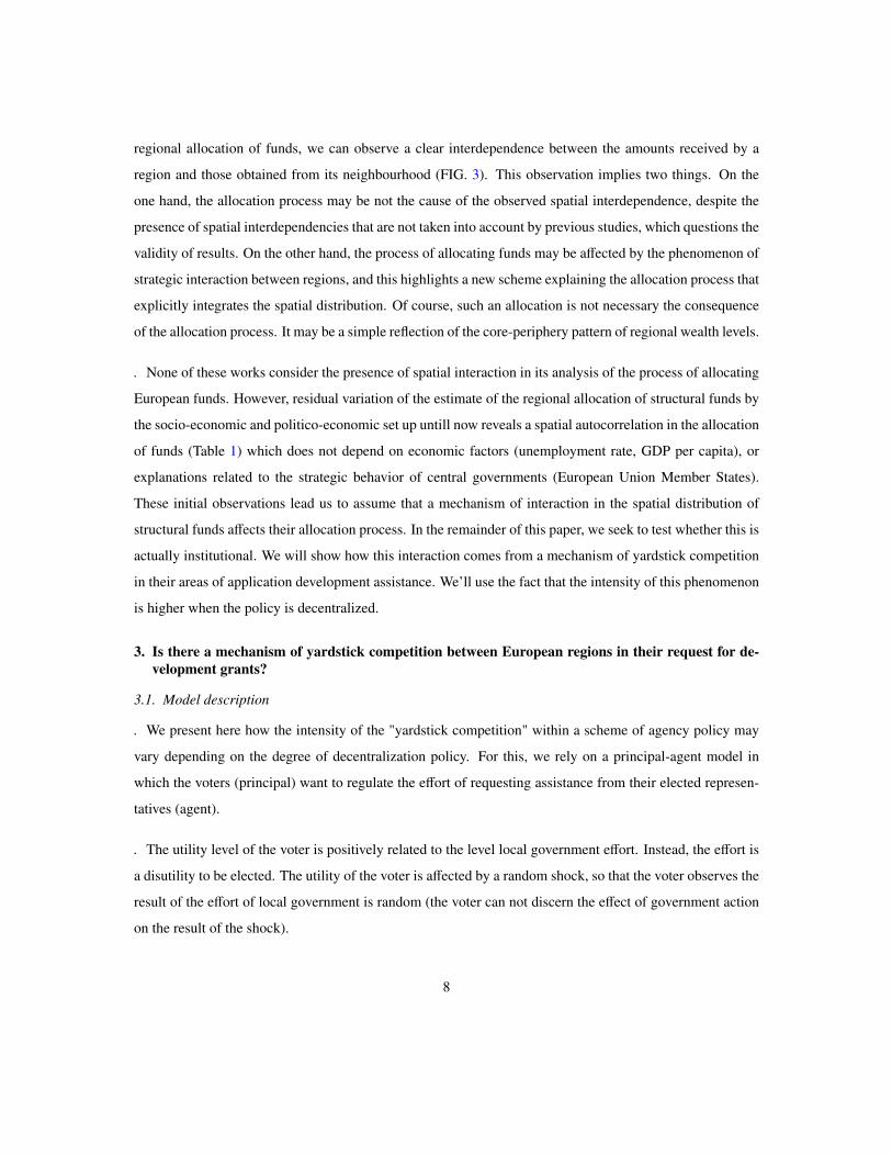
. However, when we depict the allocation of structural funds (and not mere eligibility for Objective 1 funds)

depending on two main socio-economic determinants (GDP per capita and unemployment rate), we can

observe that regions with similar socio-like economic benefit do not necessarily have the same amount of

Community subsidies. We observe indeed a negative relationship between the GDP level and the regional

amount of funds received (FIG. 1). However, when we split our sample program between Objective 1 and

other regions, this relationship does not seem to be obvious to the subsample of Objective 1 regions (the two

left quadrants, Fig. 1) . The level of regional wealth does not appear as a precise criterion for the allocation

of structural funds within Objective 1 program. Indeed, there are wide disparities in the allocation of funds

for similar levels of wealth (e.g. ITF5 and ITF3 or ES43 and PT18). This leads us to underline that once

the eligibility criterion is adopted, the allocation of funds among the regions of Objective 1 is determined

from other considerations than the level of wealth per capita. Unlike the Swedish system, the level of wealth

is only a threshold, and does not guarantee equal "treatment" for regions of the same levels of wealth. The

allocation of funds among regions that are not eligible under Objective 1, however, seem more sensitive to

the level of wealth. We can note the "under" allocation of some british (UKJ and UKH) and Belgium (BE23

and BE25) regions.

4

AT11BE32

DE3

DE4DE8

DEDDEGES11ES12ES13ES41

ES42

ES43

ES52

ES61ES62ES7

FR3

FR83GR11

GR12

GR13

GR14GR21 GR22

GR23GR24

GR25

GR3

GR41GR42

GR43

IE

ITF1

ITF2

ITF3ITF4

ITF5

ITF6

ITG1

ITG2NL23

PT11

PT15

PT16PT17

PT18 UKD

UKM

UKN

55.

56

6.5

77.

5O

bjec

tive1

199

4-99

spe

ndin

g (lo

g)

8.5 9 9.5 10GDP per capita 1989-91 (log)

AT12AT22

AT31

AT32AT33AT34

BE1BE21

BE22

BE25

BE33

BE34

DE5

DE6

DE7DEB

DEC

DEF

DK

ES21ES22ES23

ES24

ES3

ES51

ES53 FI2FR21FR22FR23

FR24

FR25FR26FR41

FR42

FR43FR51FR52FR53FR61FR62FR63

FR71

FR72FR81

FR82

ITC1ITC2

ITC3

ITC4

ITD3ITD4

ITD5ITE1

ITE2

ITE3

ITE4NL12NL21

NL22NL34

NL41NL42

SE04

SE07SE08

SE09SE0A

UKC

UKF

UKH

UKI

UKJ

UKK

12

34

56

Oth

er 1

994-

99 s

pend

ing

(log)

9 9.5 10 10.5GDP per capita 1989-91 (log)

AT11BE32

DE3

DE4DE8

DEDDEGES11ES12

ES13ES41

ES42

ES43

ES52

ES61ES62ES7

FR3

FR83GR11

GR12

GR13

GR14GR21 GR22

GR23GR24

GR25

GR3

GR41GR42

GR43

IE

ITF1

ITF2

ITF3ITF4

ITF5

ITF6

ITG1

ITG2 NL23

PT11

PT15

PT16PT17

PT18 UKD

UKM

UKN

55.

56

6.5

77.

5O

bjec

tive1

200

0-20

06 s

pend

ing

(log)


AT12

AT13

AT21AT22

AT31

AT32

AT33AT34BE1

BE21

BE22

BE23

BE25

BE33

DE1

DE2

DE5

DE6

DE7

DE9DEADEB

DECDEF DK

ES21ES22

ES23ES24

ES3

ES51ES53

FI2

FR1

FR21FR22FR23

FR24

FR25FR26FR41

FR42


FR71

FR72

FR81FR82

ITC1

ITC2

ITC3

ITC4ITD3ITD4ITD5ITE1

ITE2ITE3ITE4

ITF1UKCUKG

UKH UKI

UKJ

12

34

56

Oth

er 2

000-

06 s

pend

ing

(log)


Figure 1: Correlation between structural funds and regional income

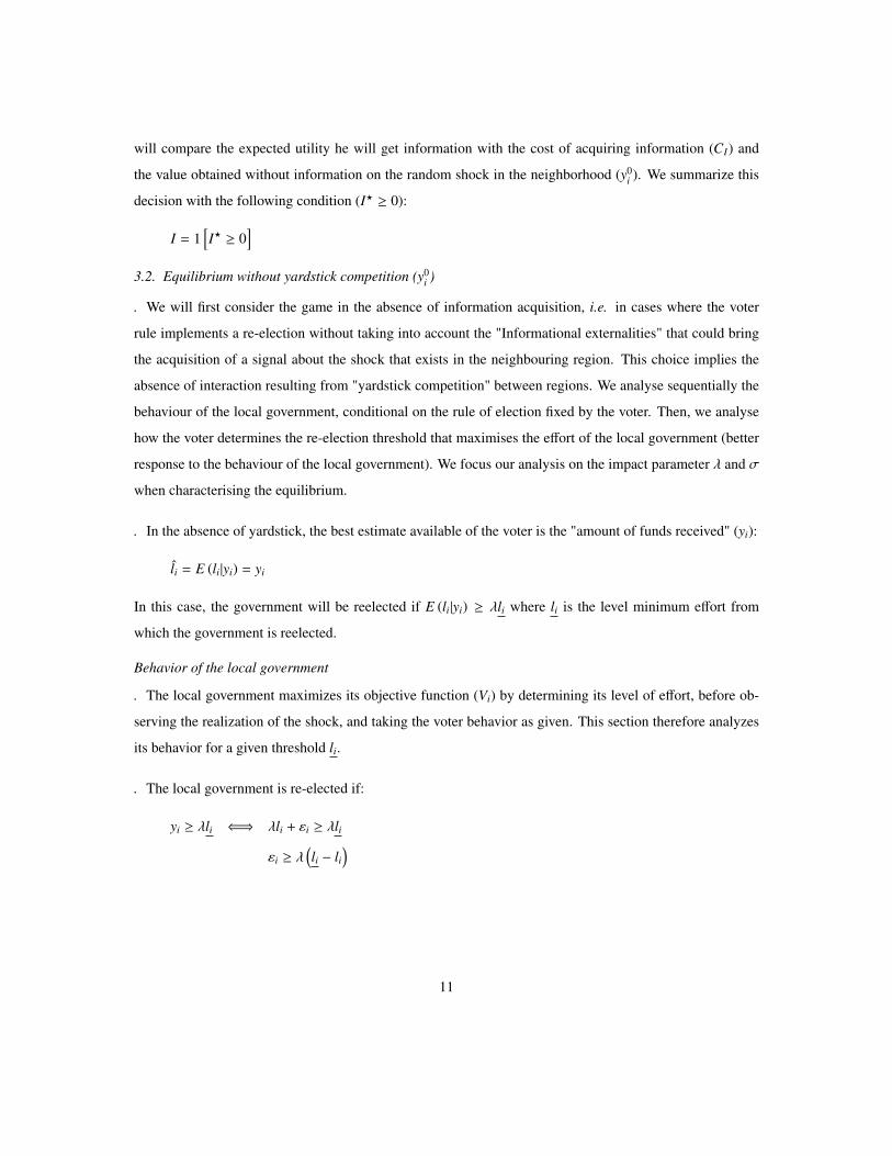
. We can observe a positive relationship between the subsidies received and the unemployment rates of

regions, regardless of the program in which they participate (FIG. 2). However, regions are widely dispersed

around the trend, so that unemployment rates for similar amounts of money received varies greatly (e.g.

UKK and PT15; ITC2 and AT13). These intuitions are confirmed by the results of a regression on all of

these factors (see table 1, p. 24). Note that the explanatory power of these factors is limited to 50% of the

variation in the amount of funds.

2.2. What is the influence of the negotiation process? Politico-economic determinants of the allocation offunds

. The section 2.1 depicts the following findings: the traditional criteria are insu!cient to adequately describe

the process of allocating European funds. According to the "Public Choice" theory, the procedures for the

preparation and implementation of such a public policy could explain the distortion of the allocation relative

to what would have been produced by criteria "socio-economic".

5

AT11 BE32

DE3

DE4DE8

DEDDEGES11ES12

ES13ES41

ES42

ES43

ES52

ES61ES62ES7

FR3

FR83GR11

GR12

GR13

GR14GR21GR22

GR23GR24

GR25

GR3

GR41GR42

GR43

IE

ITF1

ITF2

ITF3ITF4

ITF5

ITF6

ITG1

ITG2NL23

PT11

PT15

PT16PT17

PT18UKD

UKM

UKN

55.

56

6.5

77.

5O

bjec

tive

1 19

94-9

9 sp

endi

ng (l

og)

2 4 6 8 10Unemployment rate 1994

AT12AT22AT31

AT32AT33AT34

BE1BE21

BE22

BE25

BE33

BE34

DE5

DE6

DE7DEB

DEC

DEF

DK

ES21ES22 ES23

ES24

ES3

ES51

ES53FI2FR21FR22FR23

FR24

FR25FR26FR41

FR42

FR43 FR51FR52FR53 FR61FR62FR63

FR71

FR72FR81

FR82

ITC1ITC2

ITC3

ITC4

ITD3ITD4

ITD5ITE1

ITE2

ITE3

ITE4NL12NL21

NL22NL34

NL41NL42

SE04

SE07SE08

SE09SE0A

UKC

UKF

UKH

UKI

UKJ

UKK

12

34

56

Oth

er 1

994-

99 s

pend

ing

(log)


AT11

BE32DE3

DE4DE8DEDDEG

ES11

ES12

ES13

ES41ES42

ES43

ES52

ES61ES62 ES7FI13

FR3

FR83

GR11

GR12

GR13

GR14GR21GR22

GR23GR24GR25

GR3

GR41GR42

GR43IEITF2

ITF3ITF4

ITF5ITF6

ITG1ITG2

NL23

PT11

PT15

PT16PT17

PT18SE08

UKDUKE

UKK

UKL

UKM

UKN

56

78

9O

bjec

tive

1 20

00-0

6 sp

endi

ng (l

og)


AT12

AT13

AT21AT22

AT31

AT32

AT33AT34BE1

BE21

BE22

BE23

BE25

BE33

DE1

DE2

DE5

DE6

DE7

DE9DEADEB

DECDEFDK

ES21ES22ES23

ES24

ES3

ES51ES53

FI2

FR1

FR21FR22 FR23

FR24

FR25FR26FR41

FR42


FR71

FR72

FR81FR82

ITC1

ITC2

ITC3

ITC4ITD3ITD4ITD5 ITE1

ITE2ITE3 ITE4

ITF1 UKCUKG

UKH UKI

UKJ

12

34

56

Oth

er 2

000-

06 s

pend

ing

(log)


Figure 2: Correlation between structural funds and unemployment rate

. Kemmerling and Bodenstein (2006) were the first ones to show that although poorer areas receive more

regional funds, "being poor" is not a "su!cient predictor" to explain the amount of funds received by a

region. While reviewing the allocation of structural funds in several Member States, they show that the left-

wing regional are more e"ective to put pressure on their central governments and the Commission and that

they obtain more subsidies than those of regional right-wing parties. This finding is supported by Bodenstein

and Kemmerling (2008) and Bouvet and Dall’erba (2010), who also find that areas where margins are low

electoral advantage to receive EU funds. The work of Carrubba (1997) to establish a population relatively

"Euro-skeptic" in a region increases the amount of structural funds that the region receives. The reason given

by the author is that EU funds are used to increase support of public opinion in favor of the EU, and prevent

the feeling of euro-skepticism hinders the pursuit of European integration. All these studies highlight the

influence of politico-economic determinants on the allocation of funds.

. Bodenstein and Kemmerling (2008) tried to analyze the impact of patronage on the regional distribution

of structural funds. Their empirical analysis shows that the 2000-06 allocation is a"ected by the intensity

of electoral competition in national elections for the regions benefiting from Objective 2, while the intensity

6

seems to be a significant factor in the allocation of Objective 1 funds.

. Bouvet and Dall’erba (2010) tested a set of politico-economic factors with a model on censored data (To-

bit). The authors di"erentiate the allocation of funds received for Objective 1 of the Objective 2 and 3.

While other articles use national political data (Carrubba, 1997) or only regional ones (Kemmerling and Bo-

denstein, 2006), Bouvet and Dall’erba (2010) also characterized the influence of politico-economic factors

at the national level, from specific at the regional level. Overall, their results suggest that the allocation of

funds is influenced by political considerations, but that the influence of national and regional characteristics

varies depending on whether the region belongs to the Objective 1 set or not.

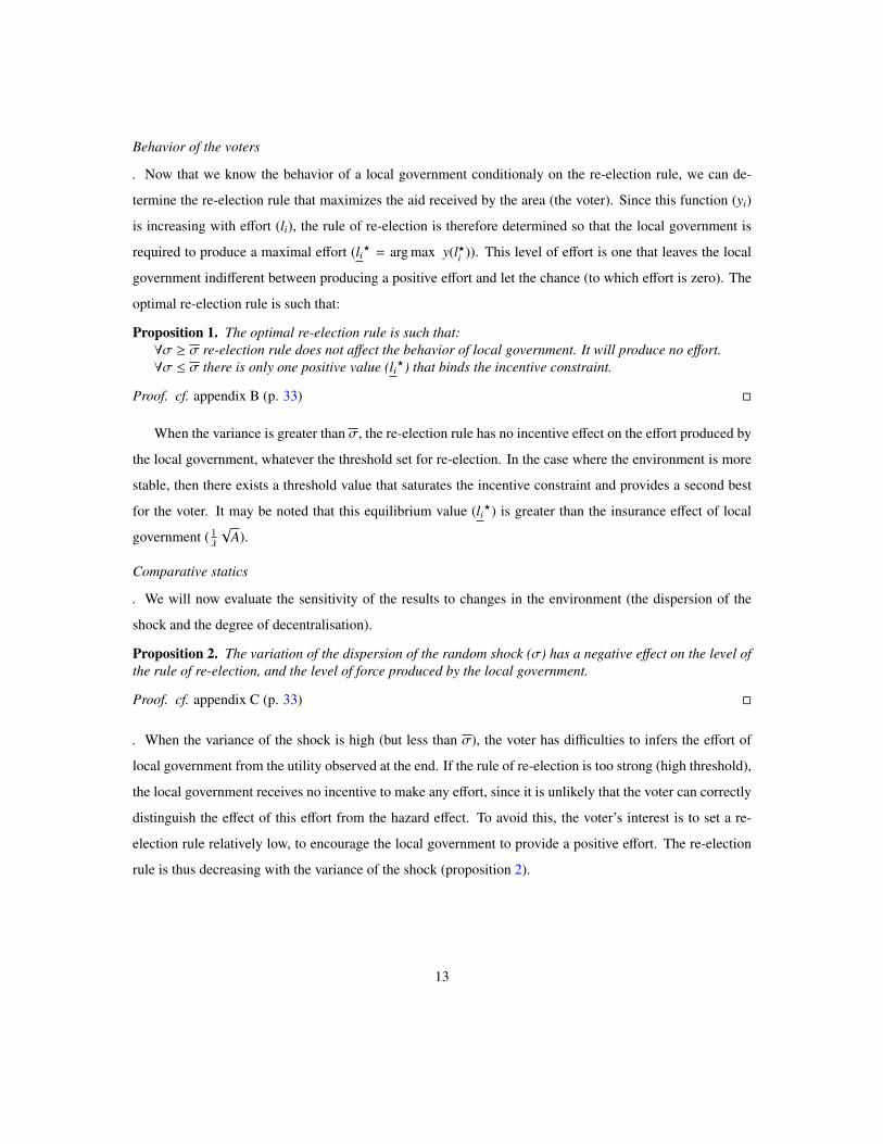
The 25% most endowed in structural funds p.c.3th quartile2th quartileThe 25% least endowed in structural funds p.c.

Figure 3: Regional allocation of structural funds (per capita, 2000-06)

2.3. Spatial interdependence in structural fund allocation: bridging a gap?

. Although these studies have greatly advanced our understanding of the process for allocating Structural

Funds, none considers the presence of spatial interdependence in this allocation. Indeed, by mapping the

7

regional allocation of funds, we can observe a clear interdependence between the amounts received by a

region and those obtained from its neighbourhood (FIG. 3). This observation implies two things. On the

one hand, the allocation process may be not the cause of the observed spatial interdependence, despite the

presence of spatial interdependencies that are not taken into account by previous studies, which questions the

validity of results. On the other hand, the process of allocating funds may be a"ected by the phenomenon of

strategic interaction between regions, and this highlights a new scheme explaining the allocation process that

explicitly integrates the spatial distribution. Of course, such an allocation is not necessary the consequence

of the allocation process. It may be a simple reflection of the core-periphery pattern of regional wealth levels.

. None of these works consider the presence of spatial interaction in its analysis of the process of allocating

European funds. However, residual variation of the estimate of the regional allocation of structural funds by

the socio-economic and politico-economic set up untill now reveals a spatial autocorrelation in the allocation

of funds (Table 1) which does not depend on economic factors (unemployment rate, GDP per capita), or

explanations related to the strategic behavior of central governments (European Union Member States).

These initial observations lead us to assume that a mechanism of interaction in the spatial distribution of

structural funds a"ects their allocation process. In the remainder of this paper, we seek to test whether this is

actually institutional. We will show how this interaction comes from a mechanism of yardstick competition

in their areas of application development assistance. We’ll use the fact that the intensity of this phenomenon

is higher when the policy is decentralized.

3. Is there a mechanism of yardstick competition between European regions in their request for de-velopment grants?

3.1. Model description

. We present here how the intensity of the "yardstick competition" within a scheme of agency policy may

vary depending on the degree of decentralization policy. For this, we rely on a principal-agent model in

which the voters (principal) want to regulate the e"ort of requesting assistance from their elected represen-

tatives (agent).

. The utility level of the voter is positively related to the level local government e"ort. Instead, the e"ort is

a disutility to be elected. The utility of the voter is a"ected by a random shock, so that the voter observes the

result of the e"ort of local government is random (the voter can not discern the e"ect of government action

on the result of the shock).

8

. This result is an imperfect signal of the lobbying activity performed by the local government. We highlight

that the acquisition of a more specific example of the shock that occurred in neighbouring regions, allows

the voter to determine a more restrictive rule for re-election, urging the Government to greater e"ort and

thus increase the voter’s expected utility. We show that the decision to acquire this signal increases with

the degree of policy decentralization, at least for an environment su!ciently stable for incentives linked to

the vote to be e"ective, but in which the variance of the shock is large enough for the marginal benefit of

acquiring information to be positive.

Objective function of the voter

. The utility for the voter that the government gets subsidies is written as follows:

y(li, !i) = "li + !i (1)

. This utility is directly related to the level of e"ort for applying for subsidies from local government (li).

The e"ect of the e"ort of local government on the utility of the voter is weighted by the degree of policy

decentralization ("). In our case, the benefit derived by the voter is confused with the amount of funds

allocated to their region of residence.

. Finally !i is a random shock (economic, determinants not controlled by local government). We will

consider that the design of the shock is perfectly correlated between the regions (Besley and Case, 1995).

The parameter " is the degree of decentralization of the cohesion policy. As its value depends on a third

institution (Member State), we consider its behavior as exogenous, and not indexed. This setting means that

the impact of the e"ort of local government is increasing with the degree of decentralization. Somehow, we

consider the impact of the actions of local governments on the welfare of the voters even more important

that skills are decentralized. The voter knows what degree of decentralization and takes into account when

determining the direct rule re-election.

Objective function of the local government

. The local decision-maker makes a profit (R) reelection (prestige, ego etc...). His (expected) welfare func-

tion depends on his re-election as follows:

Vi = Rp(li) " li (2)

where p(li) is the probability of re-election in the level of e"ort of the local government in its business

application support (li). Similarly to most principal-agent models, we consider li as a disutility for local

decision-maker (opportunity cost, for example).

9

Reelection rule

. The voter of region i sets a minimum threshold of well-being at the end of period over which the local

government is re-elected (yi). The control variable on which the re-election rule applies an incentive remains

the government’s e"ort: it is quite equivalent to reason with a minimum level of e"ort (li). The level of

government e"ort is not known to the voter. However, it can be inferred (l̂i) according to the information

available to the voter. Generally, a local government shall be re-elected if and only if:

"l̂i + !i # "li

The voter considers the degree of decentralization of political by weighting with " the limits set, so does not

ask for the balance of benefit to the local government e"ort when the degree of decentralization is low, all

things being equal. Otherwise, it would be forced to make an e"ort greater than his marginal contribution

(definition of ") in the utility of voters is low.

Timing of the game

. The di"erent steps of the game are as follows:

0. Choice to acquire information on the impact of the neighbouring region (I)

1. Commitment on the reelection rule (threshold, li)

2. Choice of e"ort by local government (li)

3. Realizations of random shocks (!i !"i)

4. Obervations ex post of outcomes (yi y"i)

5. Reelection or not of the government of the region i.

Information structure

. We are in a situation where the information structure depends directly on the voter’s choice whether to

acquire a signal on the realisation of the shock in the neighbouring region. This information provides to the

voter, when the election period occurs (stage 5 of the game), a more accurate estimate of the e"ort supplied

by his own government. From the relationship of agency policy previously presented, we can define the

condition under which a voter of region i decides to acquire information on the realisation of the shock in

the neighbouring region.

. We represent the result related to the decision of the voter by a dichotomous variable I that takes the value

1 when the voter acquires the signal and 0 otherwise. To decide if it acquires information (y1i ), the voter

10

will compare the expected utility he will get information with the cost of acquiring information (CI) and

the value obtained without information on the random shock in the neighborhood (y0i ). We summarize this

decision with the following condition (I# # 0):

I = 1!I# # 0

"

3.2. Equilibrium without yardstick competition (y0i )

. We will first consider the game in the absence of information acquisition, i.e. in cases where the voter

rule implements a re-election without taking into account the "Informational externalities" that could bring

the acquisition of a signal about the shock that exists in the neighbouring region. This choice implies the

absence of interaction resulting from "yardstick competition" between regions. We analyse sequentially the

behaviour of the local government, conditional on the rule of election fixed by the voter. Then, we analyse

how the voter determines the re-election threshold that maximises the e"ort of the local government (better

response to the behaviour of the local government). We focus our analysis on the impact parameter " and $

when characterising the equilibrium.

. In the absence of yardstick, the best estimate available of the voter is the "amount of funds received" (yi):

l̂i = E (li|yi) = yi

In this case, the government will be reelected if E (li|yi) # "li where li is the level minimum e"ort from

which the government is reelected.

Behavior of the local government

. The local government maximizes its objective function (Vi) by determining its level of e"ort, before ob-

serving the realization of the shock, and taking the voter behavior as given. This section therefore analyzes

its behavior for a given threshold li.

. The local government is re-elected if:

yi # "li $% "li + !i # "li

!i # "#li " li

$

11

Noting # be the distribution function of standard normal distribution and variance $2, the probability of

re-election of local government according to the applied load is given by1:

p(li) = 1 " #%&&&&&&'"#li " li

$

$

())))))*

The local government program is written as follows:

maxli

+,,,,,,-R

%&&&&&&'1 " #

%&&&&&&'"#li " li

$

$

())))))*

())))))* " li

.//////0

Lemma 1. Let A = 2$2ln( "R$&

2%), $ = "R&

2%and we define the incentive condition IC(A,$) by:

"#%&&&&'"&

A$

())))*R "

&A"# li " #

1"li$

2R

The level of e!ort produced by the local government is:

• '$ # $ l#i = 0,

• '$ ( $ l#i = li + 1"

&A when the IC(A,$) is binded , otherwise l#i = 0.

Proof. cf. appendix A (p. 32) !

. When the variance is very large (over $), the local government knows that its e"ort was very unlikely to

have a significant impact on the welfare of voters. Ultimately, this welfare is determined by the realization

of the shock. Therefore, the local government considers preferable to let the chance to act rather than an

e"ort that will not be "much-valued" because of its low impact on the utility of voters.

. For a lower level of variance, the local government chooses between a positive e"ort and leaves it to

chance. His choice is subject to the constraint of re-election (li), whose level is determined by the elector.

It is now important to note that the local government does not provide an equivalent e"ort on the threshold

of re-election, but provides a slightly higher e"ort in order to cover the realization of a shock especially

important ( 1"

&A). We define from now on this term as the e"ect of local government self-protection.

1the probability of re-election can be written as Pr(y # y) = 1"Pr(!i # "#li " li

$), !i follows a standard normal law with a variance

$2.

12

Behavior of the voters

. Now that we know the behavior of a local government conditionaly on the re-election rule, we can de-

termine the re-election rule that maximizes the aid received by the area (the voter). Since this function (yi)

is increasing with e"ort (li), the rule of re-election is therefore determined so that the local government is

required to produce a maximal e"ort (li# = arg max y(l#i )). This level of e"ort is one that leaves the local

government indi"erent between producing a positive e"ort and let the chance (to which e"ort is zero). The

optimal re-election rule is such that:

Proposition 1. The optimal re-election rule is such that:'$ # $ re-election rule does not a!ect the behavior of local government. It will produce no e!ort.'$ ( $ there is only one positive value (li#) that binds the incentive constraint.

Proof. cf. appendix B (p. 33) !

When the variance is greater than $, the re-election rule has no incentive e"ect on the e"ort produced by

the local government, whatever the threshold set for re-election. In the case where the environment is more

stable, then there exists a threshold value that saturates the incentive constraint and provides a second best

for the voter. It may be noted that this equilibrium value (li#) is greater than the insurance e"ect of local

government ( 1"

&A).

Comparative statics

. We will now evaluate the sensitivity of the results to changes in the environment (the dispersion of the

shock and the degree of decentralisation).

Proposition 2. The variation of the dispersion of the random shock ($) has a negative e!ect on the level ofthe rule of re-election, and the level of force produced by the local government.

Proof. cf. appendix C (p. 33) !

. When the variance of the shock is high (but less than $), the voter has di!culties to infers the e"ort of

local government from the utility observed at the end. If the rule of re-election is too strong (high threshold),

the local government receives no incentive to make any e"ort, since it is unlikely that the voter can correctly

distinguish the e"ect of this e"ort from the hazard e"ect. To avoid this, the voter’s interest is to set a re-

election rule relatively low, to encourage the local government to provide a positive e"ort. The re-election

rule is thus decreasing with the variance of the shock (proposition 2).

13

. The e"ect of the variation of $ on the e"ort of local government is more complex. Indeed, this e"ort is

determined by the sum of the e"ects of the threshold for re-election and the e"ect of insurance, which also

depends on $. If the threshold for re-election increases with the variance of the shock, the insurance e"ect

is first increasing and then decreasing with $. If the dispersion of the shock is low, then the insurance e"ect

increases with $: the local government will find better to hedge against adverse shocks. From a certain level

of variance, the cost of insurance becomes too large relative to the earnings so that the insurance e"ect then

decreases with $. For $ ( $ this second e"ect is always dominated by the e"ect of $ on the threshold of

re-election. Therefore, the e"ort of local government decreases with the variance.

Proposition 3. The variation in the degree of decentralization (") has a positive e!ect on the rule of re-election and on the force produced by the local government for R > 1.

Proof. cf. appendix D (p. 35) !

Corollary 1. The variation in the degree of decentralization (") has a positive e!ect on the utility of thevoter (yi). The variation of the dispersion of the random shock has a negative e!ect on the utility of the voter.

Proof. cf. appendix D (p. 35) !

. For a re-election rent greater than unity, the threshold for re-election increases with the degree of decen-

tralisation. As soon as the gain of the local government related to his re-election is su!ciently large (R > 1),

then the voter is better to establish a re-election rule even more restrictive when the degree of decentralisa-

tion is increasing. The more important the weight of the action of local government is in the utility of the

voter, the more the later is interested to set a high threshold.

. The e"ect on the e"ort of local government is more ambiguous. In this case, we can prove (for all values

of $ ( $) that the e"ect of the degree of decentralization through the threshold of re-election continues to

dominate the resulting e"ect of Insurance ( 1"

&A). When the dispersion of the impact is relatively low, the

e"ort of the local government is growing with the degree of decentralization (the e"ect through the threshold

of re-election dominates). For a fairly stable environment, the local government is interested in increasing

his e"ort because the gain of a re-election is higher than the cost of insurance.

3.3. Equilibrium under yardstick competition (E&i

!yC

i

"= y1

i )

. In this section, we analyze the equilibirum of the game between the local government and the voter when

the voter decides to acquire some information (a signal) on the shock realization in the neighbouring region.

14

The signal allows the voter to know with greater precision the realisation of the shock occurred in his own

region, and thus the e"ort of his own government. The signal received by the voter is:

&i = !"i + µi

where !"i a standard normal distribution with a variance $2, µi is a white Gaussian noise (µi ) N(0, 1))

The joint distribution (!"i, &i) is determined by the distribution parameters of the two random variables and

their correlation ('): (!"i, &i) ) N(0, 0,$2,$2, ') And distribution of !"i knowing &i is written: !"i|&i )N('$$&i,$2(1 " ')2) Moreover, similarly to Besley and Case (1995), we consider the case where the reali-

sation of the shocks between regions is perfectly correlated: E3!i|&i4= E3!"i|&i

4= '&i The voter considers

the level of e"ort as follows:

l̂i = yi " E3!i|&i4

l̂i = li + !i " '&i

The re-election rule is now defined by:

"li + !i " '&i # "li

The local government knows that if re-elected:

!i " '&i # "#li " li

$

Define Hi = !i " '&i, the distribution of a sum of normal random variables is itself normal:

Hi ) N(0,$2(1 " '2)5!!!!!!67!!!!!!8(2

)

The maximization program of the local government writes similarly to the previous one, where ( replaces

$.

Lemma 2. Define Z = 2(2ln( "R$&

2%), $ = "R&

2%the incentive constraint IC(A,$) below:

"#%&&&&'"&

Z(

())))*R "

&Z"# li " #

1"li(

2R

The level of e!ort by the local government is:

• '( # $ l#i = 0,

• '( ( $ l#i = li + 1"

&Z when the incentive constraints are satisfied, otherwise l#i = 0.

15

Proof. cf. proof of Lemma 1 (p. 32). !

The voter will determine the threshold value of re-election that induces the maximum e"ort produced by

the local government.

Proposition 4. The optimal re-election rule is such that: '( # $ the re-election rule does not a!ect thebehaviour of the local government. He will produce no e!ort. '( ( $ there is only one positive value (li#)that binding the incentive constraint.

Proof. cf. proof of proposition 1 (p. 33) !

. The acquisition of the signal by the voter implies that the latter has more accurate information on the level

of e"ort of the local government. Therefore, the variance (2 is lower in the case where the local government

is in competition than in the benchmark case ($2). The e"ect of the acquisition of the signal acts as if the

voter would have achieved a reduction of the variance of the random shock. Through this mechanism, we

can consider that the variance is an inverse measure of "verifiability" of the action of the local government.

Proposition 5. The situation of yardstick competition from the local government, resulting from the acquisi-tion by the voter of a signal increases the minimum e!ort required by the voter, the e!ort produced by the lo-cal government and therefore the utility of the voter. For an intermediate level of $ ( R&

2%e"

(R"1)2 ( $ ( $e"

32 ),

the e!ect of a change in the degree of decentralisation on the threshold of re-election e!ort and the localgovernment is higher in the case of yardstick competition.

Proof. cf. appendix E (p. 36) !

. The situation of yardstick competition brings greater utility to voters. The latter have, with acquisition

of a signal, a better estimate of the e"ort exerted by the local government. From this mechanism, they can

determine a stricter re-election rule. Similarly, the local government knows that by providing a high e"ort,

he is more likely to be re-elected in yardstick competition case, because the e"ect induced by his e"ort is

easily di"erentiated from the shock’s one.

. The marginal e"ect of the degree of decentralization on the threshold of re-election and on the govern-

ment’s e"ort is also higher in yardstick competition environment, at least for values close to the threshold $.

Reducing uncertainty about the action of local government can better discern the e"ect of e"ort on the e"ect

of hazard. By definition, this e"ort is particularly important for the utility of the voter when the degree of de-

centralization is high. Consequently, the marginal benefit for the voter to encourage the local government to

produce an e"ort is even higher when the yardstick competition mechanism provides a better understanding

of the action of local government (reduced variance). We show that this is true at least close to the threshold.

16

3.4. Decision to acquire information with an exogenous fixed cost (I#)

. The voter’s choice to acquire the information necessary to more precisely control the activity of his local

government depends on the following condition:

I = 1!E&i

!yC

i

""CI " y0

i # 0"

This means that the gain in expected utility (E&i

!yC

i

"" y0

i ) must be greater than the cost of acquiring this

information (CI).

Proposition 6. Assuming that this cost is fixed and exogenous, the voter decides to acquire information at acost below the following:

CI = E&i

!yC

i

"" y0

i

Proof. cf. appendix F (p. 38) !

. From this result, it is clear that the voter’s decision to acquire the signal is related to the degree of decen-

tralisation of the policy (by the e"ect of " on yi). If the degree of decentralization does not directly a"ect

the cost of acquiring information, the threshold value that switches the voter’s decision is a"ected by the

value of ". The close link between the decision to acquire information and the degree of decentralization

comes from the expected gain in utility term that generates the acquisition of information. When the degree

of decentralization is low, the weight of local government activity is usually low, the gain that would provide

better control of this activity is therefore also low. Gradually, as the degree of decentralization is increasing,

the gain expected from the acquisition of the signal increases and the cost threshold below which the voter

decides to acquire the signal also increases.

. Finally, we need only to determine, based on previous results, the e"ect of a change in the degree of

decentralization on the voter’s decision to acquire information on the shock occurred in the neighbouring

region. This decision depends solely on the e"ect of the variation of " on the condition of acquiring the

information (I#)):

)I#

)"=)y1

i

)"")y0

i

)"

Proposition 7. For an intermediate level of $ ( R&2%

e"(R"1)

2 ( $ ( $e"32 ), an increasing degree of decentrali-

sation always a!ects positively the decision to aquire information ( )I#

)" > 0.)

Proof. cf. appendix G (p. 38) !

17

. This proposal shows that the voter’s decision to acquire information on the realization of shocks in neigh-

bouring regions (and implement a "contract" under yardstick competition) is always increasing with the de-

gree of decentralization of the policy, at least when the variance of the shock is close to the variance threshold

beyond which the government exerts no e"ort. That is exactly around this threshold that the marginal benefit

of acquiring information is the highest. Close to the threshold, the marginal benefit is always increasing with

the degree of decentralization, since it allows voters to encourage their local government to pass a null e"ort

toward a positive e"ort.

4. Empirical analysis

. The main di!culty in our empirical analysis is to ensure that the spatial interactions of the allocation of

structural funds do originate from a mechanism of yardstick competition. Similarly to research the origin of

fiscal externalities, it is logical to consider that these spatial interdependencies can be the result of spillover

e"ects of economic or even unobserved shock that propagates through a spatial process.

. Our theoretical model shows that the voter decision to acquire information increases with the degree

of decentralization. When the degree of decentralization is low, the weight of the decision of the local

government in the utility of voters is low. The gain that would provide better control of its activity is

therefore low. Gradually, as the degree of decentralization increases, the expected gain associated with the

acquisition of information (and to use yardstick competition) increases. For a decentralized system, the

voter of each region has a stronger incentive to acquire information, which allows it to better discipline their

own government. The e"ort of this local government will be higher, leading this region to obtain larger

amounts. This reasoning breeding within each region, we obtain a positive e"ect on the amount of funds

received by a region of the amounts received by its neighbors for each region whose system of governance

is decentralized. This prediction thus implies that the intensity of spatial interactions (caused by yardstick

competition) is stronger when the policy is decentralized.

. The proposition 7 (section 3) highlights how incentives may change depending on the structure of imple-

mentation of the policy. These results allow us to infer that if the interactions are caused by the mechanism

of yardstick competition, then their intensity should be higher for regions whose management is delegated to

local authorities (decentralized system). The fact that the choice of the governance structure of the policy is

determined by each Member State, will allow us to identify whether the origin of the interaction is e"ectively

an institutional ("yardstick competition") by providing us with a change in the type of structure used in place

18

(section 4.1). Specifically, we will use the heterogeneity between member states in their decision to dele-

gate the implementation of funds to local authorities (decentralized system) or not (centralized-decentralized

system.

4.1. Incentives of local government and cohesion policy governance

. The decision to delegate the management of structural funds to local elected o!cials is determined by

each Member State. We can distinguish three types of choice within the EU 15 for the programming period

2000-06 (Bachtler, 2008).

. Some of the member states chose to keep the responsibility for cohesion policy at the central level. In

practice, it relies heavily on decentralized services to ensure a more close to citizens. Under this regime, we

assume that the local governments have no incentive to engage in lobbying activity because voters can clearly

monitor the activities of local government regarding this policy. This choice is often linked to traditionally

"centralised" states. Thus, this scheme has been introduced by France, UK, Ireland, Portugal and Greece.

. The second regime corresponds to a decentralised management of funds. In this case, the policy man-

agement is delegated to local governments. Comparing the results of the process of allocating funds based

on lobbying is easier. Section 3 tells us that voters are more inclined to use the mechanism of yardstick

competition when the degree of decentralization policy is high. This is because the marginal contribution to

the e"ort of local government is by definition more powerful when the degree of decentralization is high.

We expect that the incentive for local governments is higher under decentralized situations. This choice

corresponds mainly to the "federal" Member States like Germany, Austria, Belgium, Denmark, Finland, the

Netherlands and Sweden. Even beyond the informational aspects illustrated by the theoretical model, voters

clearly associate the implementation of cohesion policy as an activity specific to local government, which

reinforces the e"ect of "disciplining" of the procedure for re-election.

. Finally, Spain and Italy have chosen an mixed regime. Both Member States have decided to give the

responsibility Objective 1 program to the central government and to delegate the management of other

programmes to the regional governments. For these two countries, we consider programs Objective 1 by the

centralized system while other programs will be considered under the decentralized system.

. We are aware that this categorization of governance structures is greatly simplified. The key determinant

of our study is to distinguish whether the local decision-maker (responsible for local implementation of the

policy) is an elected representative (decentralized system) or not (centralized system).

19

4.2. Estimation methods

. The models of strategic interactions between governments are generally estimated using the tools devel-

oped by spatial econometrics. There are generally two types of specifications (Anselin, 1988): the spatially

autocorrelated error model (SEM) and spatially autoregressive model (SAR). According to work Brueckner

(2003), spatially autoregressive specification is the most appropriate for estimating a reaction function after

a model of strategic interaction, whatever the origin of these interactions. Matrix form, this gives:1

S Fpop

2= * + (ECO)+ + (POL), + 'W

1S Fpop

2+ - (3)

The amount of funds received#

S Fpop

$by a region is positively correlated (' > 0) with the level received

by the neighbouring regions (W#

S Fpop

$). Each local government (noting that voters can assess his lobbying

indirectly) will be encouraged to engage in an activity of looking for grants to get as much as its neighbours.

W is the neighbourhood matrix, (ECO) and (POL) are the vectors of socio-economic and politico-economic.

. The existence of spatial interactions may still come from di"erent sources than the yardstick competition.

If one considers that di"erent regions are competing for a scarce resource (the central government grants),

then the amount of funds received by a region may be a"ected by the amounts received by others. One can

logically assume that there is an interdependence of policy choices other than the mechanism of yardstick

competition. It may come with similar characteristics were not taken into account in the specification or

even a common shock that the di"usion support is space. Two estimation methods are available to enable us

to identify whether the yardstick competition is at the origin of spatial interactions.

. The first approach uses an spatial autoregressive specification in which we introduce an interaction variable

between the variable of choice of fund management system and the autoregressive variable:1

S Fpop

2= * + (ECO)+ + (POL), + 'W

1S Fpop

2+ .reg.W

1S Fpop

2+ - (4)

with reg is a dummy variable equal to 1 when the funds are managed by locally elected policymakers

(decentralized system). The coe!cient on this interactive variable is significantly positive when the yardstick

competition mechanism is at work. This approach is similar to Case et al. (1993) or Solé Ollé (2003).

Equation (4) is estimated using an instrumental variables strategy. This technique can be useful when you

suspect some variables (in addition to the spatial autoregressive term) endogenous. However, this estimator

su"ers from significant shortcomings in the estimation of a SAR. The estimated interaction e"ect may fall

outside the space in which it is defined. Moreover, its use is limited to cases where the level of funds received

by a region is not a"ected by the characteristics of its neighborhood.

20

. The second method is to estimate a model introducing two regimes in the spatial autoregressive variable:1

S Fpop

2= * + (ECO)+ + (POL), + 'reg=1MW

1S Fpop

2(5)

+'reg=0(IN " M)W1

S Fpop

2+WX/ + -

in which we estimate two e"ects of spatial interactions based on the fund management system. The above

equation is estimated using a maximum likelihood method (Allers and Elhorst, 2005). An important advan-

tage of this technique lies in the ability to control the results by the WX.

. We have to ensure that other sources of spatial autocorrelation are not influencing our results. The best

strategy would be to estimate a spatial Durbin model, including a simultaneous spatial autoregressive term,

additional variables spatially lagged and a spatially correlated error term. Unfortunately, it is not possible

to simultaneously identify all of these parameters (Elhorst and Fréret, 2009). In this case, Le Sage and

Pace (2009) explain that the least "bad" solution is to exclude the error term spatially autocorrelated for the

simple reason that this solution is the only one able to produce unbiased estimates, even if the true generating

process SAR data is a SEM or a combination of both.

4.3. Data and variables

Our dataset consists in 152 NUTS1/NUTS2 regions, grouped into 14 Member States for UE-15 over the

period 2000-2006: Austria (15 regions), Denmark (1 region), Spain (17 regions), Finland (5 regions), France

(22 regions), Greece (13 regions), Ireland (1 region), Italy (19 regions), Netherlands (12 regions), Portugal

(6 regions), Sweden (8 regions) and United Kingdoms (12 regions).

. Socio-economic data come from the "Cambridge econometrics" database. Data on structural funds re-

gional display are extracted from the 11th report on structural funds (1999). We used data from the "Eu-

ropean Election database" to build the politico-economic variables that enable us to test the assumptions

depicted in the previous section.

. The typology of management structure comes from the work of Bachter (2008). The socio-economic

variables are:

• the per capita gross domestic product (lngdp). According to the redistributive logics of the cohesion

policy, we expect a negative e"ect of this variable on the allocated funds.

21

• the unemployment rate, expressed as a percentage of the regional active population (lnunemprate). A

region having a high unemployment rate should receive more funds and we expect a positive e"ect of

this variable.

• the share of active population in the whole population, expressed as a percentage of the whole popula-

tion (lnpartactivpop). This variable permits us to control for the demographic structure of the regional

population.

• the share of agricultural employment in the total amount of jobs (lnagricemp). This variable is a proxy

for the amounts of funds received by a region for CAP subsidies. We wish to control the assumption

that high agricultural regions receive less structural funds, because they receive subsidies from the

CAP.

. Moreover, we introduce politico-economic variables to control for the possible rigging of funds allocation

by member states:

• we use the intensity of electoral competition at the regional level during parliament elections (in per-

cent) to control for "swing voter" assumption. We expect appositive e"ect of this variable because

the higher the intensity of electoral competition in a region, the higher amounts of funds she should

receive. This variable is constructed from the absolute di"erence of votes received by the two major

parties (Cdi").

• to control for regional overrepresentation on national parliaments, we introduce a variable measuring

the total number of regional seats per capita within the parliamentary majority of each member state

(majreppc). We expect a positive impact of this variable on the receipt of EU funds.

. Unfortunately, we were not able to control for the partisan hypothesis because we did not have the needed

data on the results of local elections. We consider several definitions for building the spatial weight matrix

(W). The first is defined from the notion of contiguity:9:::::::::;:::::::::<

wi j = 1 i f i and j share a common border ' i ! j

w = 0

9:::::;:::::<

otherwise

i f i = j

22

. The above spatial weight definition may appear too general in the way that the information on the amounts

of funds received is available to the citizens. Indeed, the simple notion of contiguity does not account for

cultural factors, and may limit the dissemination of needed information. The language barrier, or more

generally the borders of Member States may be an example of these factors limiting the dissemination of

information. Thus, we define the spatial interaction from membership in the same Member State:9:::::;:::::<

wi j = 1 i f i and j is included in the same Member S tate ' i ! j

w = 0 otherwise

. This definition remains highly questionable because it can also capture e"ects related to a process of direct

competition between regions within the same Member State in their funding requests. Nevertheless, we will

use this matrix to control the average e"ects level per member state of the di"erent variables to control for.

Finally, we construct a matrix combining the two matrices presented above.

4.4. Results

. In table 1, we present estimates of equation (3), without taking into account strategic interactions. As

expected, the level of wealth per capita (unemployment) a"ect negatively (positively) the amount of funds

received by a region. We can also note that the over-representation of a region within the majority parlia-

mentary of its Member State is positively associated with the amount of funds. These results are consistent

with the logic presented by Kemmerling and Bodenstein (2006), or Bouvet and Dall’erba (2010), since the

process of allocating funds is a"ected by the socio-economic factors as well as politico-economic factors

(over-representation of some regions within national majorities). These last factors are due to institutional

and political features in each Member State that lead a distortion in the fund allocation compared to a pure

redistributive allocation. However, we detect the presence of spatial autocorrelation using a Moran I test

on estimate residuals (table 1). This result supports our hypothesis on the presence of spatial interactions

between regions in the allocation of structural funds.

. To learn further about the shape of this spatial autocorrelation, we use the strategy proposed by Anselin

et Florax (1995). The strategy is to detect the the most appropriate form of spatial autocorrelation for our

model. SARMA test confirms the results of the Moran test and wrongly omitted an unknown form of spatial

autocorrelation (table 2, p. 24).

23

OLS

lngdp -0.28* -2.46*** -2.46***

(-1.61) (-5.41) (-5.41)

lnunemprate 1.45*** 0.83** 0.83**

(6.01) (2.90) (2.90)

lnpartactivpop 8.76*** 11.03** 11.03**

(2.76) (3.14) (3.14)

lnagricemp 8.77 1.91 1.91

(5.97) (1.13) (1.13)

lncdi" 0.17 0.17

(1.33) (1.33)

lnmajreppc 0.67*** 0.67***

(3.83) (3.83)

constant 1.08 21.69*** 21.69***

(1.24) (5.02) (5.02)

R2 0.41 0.59 0.59

Imoran 5.7126 2.3716 2.3716

p.v.Imoran (<0.01) (0.01) (0.01)

N 152 152 152

*, **, *** indicate respectively the significance at 10%, 5% and 1% level.

Student t are displayed in parentheses beneath the coe!cient estimates.

Table 1: Estimations without spatial interactions

Wcont LMe RLMe LMlag RLMlag S ARMA

Test statistic 1.50 3.95 2.44 4.58 4.594

p.v. 0.22 0.05 0.11 0.03 0.03

H0 " = 0 " = 0 ' = 0 ' = 0 ' = " = 0

Table 2: LM tests for spatial autocorrelation

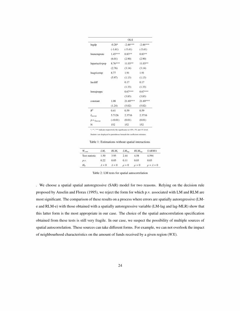
. We choose a spatial spatial autoregressive (SAR) model for two reasons. Relying on the decision rule

proposed by Anselin and Florax (1995), we reject the form for which p.v. associated with LM and RLM are

most significant. The comparison of these results on a process where errors are spatially autoregressive (LM-

e and RLM-e) with those obtained with a spatially autoregressive variable (LM-lag and lag-MLR) show that

this latter form is the most appropriate in our case. The choice of the spatial autocorrelation specification

obtained from these tests is still very fragile. In our case, we suspect the possibility of multiple sources of

spatial autocorrelation. These sources can take di"erent forms. For example, we can not overlook the impact

of neighbourhood characteristics on the amount of funds received by a given region (WX).

24

SOCIO-ECO POLITICO-ECO

IV ML IV ML

No control No control Wcont X control No control No control Wcont X control

lngdp -2.20*** -0.30* 0.07 -3.15*** -1.88*** -1.94***

(-6.67) (3.08) (0.20) (-5.17) (14.59) (14.18)

lnunemprate 0.66*** 1.44*** 1.82*** 0.54** 0.99*** 1.33***

(2.68) (33.13) (38.44) (1.97) (12.91) (16.60)

lnpartactivpop 8.14*** 8.70*** 1.26 9.51** 10.92*** 6.01

(3.05) (7.69) (0.20) (2.95) (11.04) (2.89)

lnagricemp 4.86*** 8.43*** 6.92*** 3.38** 3.39** 3.09**

(3.28) (30.33) (25.53) (2.05) (4.45) 4.03)

lncdi" 0.40*** 0.15 -0.04

(3.28 (1.52) 0.09)

lnmajreppc 0.16 0.96*** 0.39**

(1.49) (25.18) 4.14)

Wlnsfpc -0.09* 0.07 0.49*** -0.27 -0.10** 0.2**

(-1.81) (1.97) (29.71) (-1.26) (3.86) (3.85)

constant 22.53*** 1.01 0.44 31.63 15.30 18.98

Wlngdp -0.52*** -0.11

(5.73) (0.18)

Wlnunemprate -1.45*** -1.10

(12.66) (5.44)

R2 0.44 0.44

log-likehood -247.51 -215.38 -148.97 -141.81

Sargan 14.76 (0.002) 19.96 (0.001)

N 135 152 152 135 104 104

*, **, *** indicate respectively the significance at 10%, 5% and 1% level. Student t are displayed in parentheses beneath the coe!cient estimates.

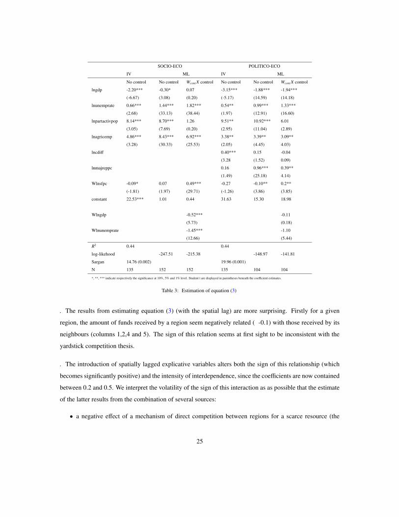
Table 3: Estimation of equation (3)

. The results from estimating equation (3) (with the spatial lag) are more surprising. Firstly for a given

region, the amount of funds received by a region seem negatively related ( -0.1) with those received by its

neighbours (columns 1,2,4 and 5). The sign of this relation seems at first sight to be inconsistent with the

yardstick competition thesis.

. The introduction of spatially lagged explicative variables alters both the sign of this relationship (which

becomes significantly positive) and the intensity of interdependence, since the coe!cients are now contained

between 0.2 and 0.5. We interpret the volatility of the sign of this interaction as as possible that the estimate

of the latter results from the combination of several sources:

• a negative e"ect of a mechanism of direct competition between regions for a scarce resource (the

25

development grants in our case)

• a negative e"ect of a mechanism of direct competition between regions for a scarce resource (the

development grants in our case)

To determine whether the second e"ect is indeed at work, we introduce the strategy described in section 4.1.

. First of all, we can note that the interpretation of results is similar, whatever the estimation method used

(cross-product estimator or model with two spatial regimes). However, the results of the Sargan test on the

method of cross product involves the rejection of a correct identification by the instruments used (p.v. equal

to 0.01). Therefore, we will focus on the results provided by the second method.

. The estimation of two regimes for the spatial lag (one for regions where management is delegated to local

government, the other not) provides results for the emergence of a mechanism of yardstick competition

between regions in the demand for development grants. Indeed, this interaction is not significant in the

case where management is delegated to local governments while the latter is significantly positive in the

case of decentralized management (0.26). The di"erence between the coe!cients of the two regimes is still

significant (table 4, "Di"").

. The introduction of WX (table 4, colonnes 3 et 4) a"ects neither the sign nor the significance of the coef-

ficient associated with the decentralised regime. The intensity of this interaction is more modest; however,

the coe!cient varies between 0.22 (when the WX are designed from the contiguity matrix) and 0.13 (when

the WX are built based on the Member State membership).

. We use a "Member state membership" matrix to determine how the variables measured in national average

may a"ect the results (table 4, column 4). We observe that the level of GDP pc national average negatively

a"ects the amount of funds received by its regions (-0.57). The average unemployment rate of Member state

seems to a"ect negatively the amount of funds received by the regions (-0.83). The WX constructed from

the contiguity matrix do not significantly a"ect the process of allocation of structural funds (table 4, column

2).

26

Cross-product Two-regime Spatial lag

IV ML

No control No control Wcont X control CX control

lngdp -2.26*** -0.19 -0.12 0.19

(-3.84) (-1.33) (-0.86) (0.75)

lnunemprate 0.78*** 1.51*** 1.26*** 1.54***

(2.94) (6.15) (5.05) (5.23)

lnpartactivpop 7.60*** 10.23*** 9.06*** 0.26

(2.67) (3.37) (3.06) (0.06)

lnagricemp 3.63** 8.32*** 6.48*** 4.91***

(2.42) (5.81) (4.20) (2.87)

lncdi" 0.16 0.10 0.14

(1.62) (1.10) (1.11)

lnmajreppc 0.14 0.29*** 0.39

(1.12) (2.70) (1.52)

spatial lag GDP -0.57*

(-1.81)

spatial lag UNEMP -0.83*

(-1.87)

Wlnsfpc*reg 0.78** regional autonomy

(2.35) no yes no yes no yes

Wlnsfpc -0.16 -0.04 0.26*** -0.05 0.22*** -0.06 0.13*

(-0.47) (-0.69) (3.16) (-0.81) (2.71) (-1.08) (1.71)

Di" -0.30 (-2.89) -0.27 (-2.63) -0.20 (-2.02)

constant -3.78** -1.67*** -1.84*** -1.42***

R2 0.57 0.45 0.49 0.54

log-likehood -243.33 -238.30 -228.52

Sargan 49.69 (0.01)

N 135 72 80 72 80 72 80


Table 4: Estimation of equations (4) and (5)

. To test the sensitivity of the interaction with the definition of the spatial weight matrix, we perform the

estimates with a spatial lag constructed using matrices "belonging to a single Member State (C)" and a com-

bination of this last matrix with the contiguity matrix (Wmixed). The interaction within the same member state

remains more intense for member state that have delegated the management of funds to local governments

(0.6).

5. Conclusion

. This paper o"ers an institutional explanation of spatial interaction of the allocation of EU structural funds.

We implement an estimation strategy to identify the proportion of interactions caused by a yardstick compe-

27

Country weights (C) Mixed weights (Wmixed)

No control CX control No control Wmixed X control

lngdp 0.06 0.18 -0.08 0.23

(0.40) (0.82) (-0.54) (0.92)

lnunemprate 1.13*** 1.68*** 1.17*** 1.48***

(4.85) (6.43) (4.66) (4.96)

lnpartactivpop 4.05 -1.44 7.87*** -0.99

(1.48) (-0.40) (2.65) (-0.24)

lnagricemp 5.89*** 5.20*** 6.58** 4.93**

(4.07) (3.44) (4.23) (2.85)

lncdi" 0.05 0.19* 0.12 0.19

(0.68) (1.68) (1.30) (1.41)

lnmajreppc 0.28*** 0.40** 0.28*** 0.36

(2.75) (1.79) (2.58) (1.37)

spatial lag GDP -0.18 -0.60*

(-0.61) (-1.88)

spatial lag UNEMP -1.29*** -0.83*

(-3.19) (-1.84)

regional autonomy

no yes no yes no yes no yes

spatial lag of lnsfpc 0.05 0.57*** 0.02 0.60*** -0.02 0.15** -0.02 0.07

(0.40) (6.49) (0.07) (6.15) (-0.29) (2.02) (-0.35) (1.08)

Di" -0.53 (-3.77) -0.58 (-2.42) -0.16 (-1.73) -0.10 (-1.05)

constant -3.18*** -3.37*** -1.27*** -0.89**

R2 0.56 0.64 0.47 0.54

log-likehood -229.72 -271.11 -239.90 -229.86

N 72 80 72 80 72 80 72 80


Table 5: Robustness to the spatial weight definition (equation (5))

tition mechanism of between regions in its demand for public aid for development. We back our empirical

identification from results of a political agency model (Sand-Zantman, 2003), where we endogeneise the

voter’s decision to use the mechanism of yardstick competition by acquiring information on the realization

of economic shocks in the neighbourhood. We show that this decision is positively a"ected by the degree

of decentralization policy. In the context of cohesion policy, the proposal identifies whether the interaction

is due to a mechanism of yardstick competition by using the choice of Member States to decentralize (or

not) the implementation of this policy. Using a spatially autoregressive specification with two regimes, we

show that the di"erence between the two regimes (one for areas where management is delegated to local

28

government, the other not) is always significant and in support of the emergence (existence) of yardstick

competition between regions in the demand for development grants.

29

Allers, M. A. and Elhorst, J. P. (2005). Tax mimicking and yardstick competition among local governments

in the netherlands.

Barro, R. J. (1986). Control of politicians. Public Choice, 14:19–42.

Besley, T. and Case, A. (1995). Incumbent behavior: Vote-seeking, tax-setting, and yardstick competition.

The American Economic Review, 85(1):25–45.

Boadway, R. and Shah, A. (2009). Fiscal Federalism. Cambridge Books.

Bodenstein, T. and Kemmerling, A. (2008). Ripples in a rising tide: Why some eu regions receive more

structural funds than others. CES Working Paper 57.

Bouvet, F. and Dall’erba, S. (2010). European regional structural funds: How large is the influence of politics

on the allocation process? JCMS: Journal of Common Market Studies, 48(3):501–528.

Brueckner, J. K. (2003). Strategic interaction among governments: An overview of empirical studies. Inter-

national Regional Science Review, 26:175–188.

Carrubba, C. J. (1997). Net financial transfers in the european union: Who gets what and why? Journal of

Politics, 59(2):469–96.

Case, A. C., Rosen, H. S., and Hines, J. R. (1993). Budget spillovers and fiscal policy interdependence :

Evidence from the states. Journal of Public Economics, 52(3):285–307.

Dotti, N. (2010). Being poor is not enough: the ’non-written" factors a"ecting the allocation of the eu

structural funds. In XXXI conferenza intalinana di scienze regionali.

Edmark, K. and Ågren, H. (2008). Identifying strategic interactions in swedish local income tax policies.

Journal of Urban Economics, 63(3):849–857.

Elhorst, J. P. and Fréret, S. (2009). Evidence of political yardstick competition in france using a two-regime

spatial durbin model with fixed e"ects. Journal of Regional Science, 49(5):931–951.

Kemmerling, A. and Bodenstein, T. (2006). Partisan politics in regional redistribution: Do parties a"ect the

distribution of eu structural funds across regions? European Union Politics, 7(3).

Le Sage, J. and Pace, R. (2009). Introduction to spatial econometrics. CRC Press Inc.

30

Salmon, P. (1987). Decentralisation as an incentive scheme. Oxford Review of Economic Policy, 3(2):24–43.

Sand-Zantman, W. (2003). Economic integration and political accountability. European Economic Review,

48(5):1001–1025.

Solé Ollé, A. (2003). Electoral accountability and tax mimicking: the e"ects of electoral margins, coalition

government, and ideology. European Journal of Political Economy, 19(4):685–713.

31

Appendix: proofs

A. Lemma 1Proof. The first order condition (FOC) provides:

)Vi)li

!= 0 * "R

#" "$$#+1"#li"li$

$

2" 1 = "R

$&

2%e"("(li"li))2/2$2 " 1 = 0

The second order condition (SOC) is:"R$3&

2%"(li " li)e"("(li"li))2/2$2

The sign of the second derivative depends on the sign of the second term ((li " li)).Si li # li the SOC is positive, which implies that the function is convexThe local government then chooses an e"ort level between zero and a level li

If the function is increasing then li0 = li.If the function is decreasing then li0 = 0.

For a nul e"ot, the government’s objective function is written:)Vli=0

)li= "R$&

2%e"("(li))2/2$2 " 1

)Vli=0

)li( 0 => "R

$&

2%e"("(li))2/2$2 ( 1

"("(li))2

2$2 ( ln=$&

2%"R

>

If $&

2%"R > 1 i.e. $ # "R

$&

2%then we always have )Vli=0

)li< 0 and li0 = 0.

If $ ( "R$&

2%we have

"("(li))2

2$2 # ln=$&

2%"R

>

Let L = $"

?2ln=$&

2%"R

>

If li eis high (greater than L) then )Vli=0

)li< 0 and li0 = 0.

If li ( li the SOC is negative, and the function is concave.The FOC is written:

"R$&

2%e""

2(li"li)2/2$2 " 1 = 0

ln( "R$&

2%e""

2(li"li)2/2$2) = 0

ln="R$&

2%

>+ ln#e""

2(li"li)2/2$2$= 0

"2(li " li)2 = 2$2ln="R$&

2%

>

Let X = "2(li " li)2

We get 2 solutions "(li " li) = +/ "?

2$2ln="R$&

2%

>

It has " > 0 but no information on the sign of (li " li).If we put a risk aversion of local government, this implies "(li " li) < 0.

"(li " li) = "?

2$2ln="R$&

2%

>

As "(li " li) < 0 we have a single solution:* l0i = li + 1

"

&A when whe let A = 2$2ln( "R

$&

2%)

32

We have "R$&

2%( 1 for $ # "R&

2%and therefore we can summarize the behavior of local government

function the threshold for re-election and conclude in all cases:l0i = 0 for $ # "R&

2%

l0i = li + 1"

&A for $ ( "R&

2%!

B. Proposition 1Proof. The level of e"ort that determines the decision rule is defined by:

Vli=l#i # Vli=0 (IC(A, $))which equivalent to:R=1 " #

="&

A$

>>" li "

&A" # R

=1 " #

="li$

>>

rearranging we get:"#="&

A$

>R "

&A" # li " #

="li$

>R

we seek li which incites local government to produce a positive e!ort.Let:F(li) = "li + #

="li$

>R " #

="&

A$

>R "

&A"

Our goal is to analyze the function F(li) to determine a value of li > 0 which binds IC(A, $).We note that:F(li) = 0 for li = "

&A"

)F)li= "1 + "R

$&

2%e""

2li2/2$2= 0

"2li2 = 2$2ln="R$&

2%

>

* l#i ="&

A" or

&A"

The SOC:d2Fd2li= " "R

$3&

2%"lie""li

2/2$2

d2Fd2li= " "R

$3&

2%"li

5!!!!!!!!!67!!!!!!!!!8e"li2/2$2

5!!67!!8

'li ( 0 # 0 # 0'li # 0 ( 0 # 0

'li ( 0 the function F is convex, and reaches a minimum in "&

A" . Furthermore, we know that the value

of this minimum is zero (F(li) = 0). Therefore F # 0 for li ( 0 and F(0) > 0. 'li # 0 F is strictly concave,so there is only one solution to the equation F(li) = 0 pour li # 0. We know that this value is greater than&

A" (since F reaches a maximum for this value).

There is a value li > 0 solution of the equation F(li) = 0 i.e. that binds the incentive constraint. We know

that this value is greater than&

A" . !

C. Proposition 2Proof. The e"ect of a variation of $ on the variation of the rule re-election e"ort and level of central gov-ernment is given by (implicit function theorem):

)li)$ = "

)F/)$)F/)li

33

Moreover, we know that )F/)li < 0 around of equilibrium.

)F)$ = " R

$2&

2%"lie""

2li2/2$2 " R@"&A($,.)$

A+. 1&

2%e"A/2$2 " A+($,.)

2"&

A($,.)@"&A($,.)$

A+=

"2$2&

Aln="R$&

2%

>+ $

2&

A+&

A

$2

="A&

A+ $

2&

A+&

A

$2

= 1&A

)F)$ = " R

$2&

2%"lie""

2li2/2$2 " R 1B2$2ln( "R

$&

2%). 1&

2%e"A/2$2

5!67!8$&

2%"R

" 2$(2ln( "R$&

2%)"1)

"2B

2$2ln( "R$&

2%)

)F)$ = " R

$2&

2%"lie""

2li2/2$2 " R$&

2%"R$&

2%B

2ln( "R$&

2%)" $(2ln( "R

$&

2%)"1)

"B

2$2ln( "R$&

2%)

)F)$ = " R

$2&

2%"lie""

2li2/2$2 " 1"B

2ln( "R$&

2%)" (2ln( "R

$&

2%)"1)

"B

2ln( "R$&

2%)

)F)$ = " R

$2&

2%"lie""

2li2/2$2 " 1"2ln( "R$&

2%)+1

"B

2ln( "R$&

2%)

)F)$ = " R

$2&

2%"lie""

2li2/2$2 "B

2ln( "R$&

2%)

"

)F)$ < 0

)li)$ = "

)F/)$)F/)li

< 0The variation of $ has a negative e"ect on li.

In addition, the e"ect of the variation of the variance of the shock on the level of e"ort is written:)li)$ =

)li)$ +

1"

@A+($,.)

2&

A($,.)

A

If A+($, .) < 0 then )li)$ < 0if A+($, .) > 0 which e!ect dominates the other?Multiplying by

)F/)li)F/)li

:)li)$ = " 1

)F/)li

=)F)$ " )F)li

1"

@A+($,.)

2&

A($,.)

A>

)F)li= "R$&

2%e""li

2/2$2 " 1

)li)$ = " 1

)F/)li

%&&&&'" R$2&

2%"lie"

"li2

2$2 " 1"B

2ln( "R$&

2%)" A+($,.)

2"&

A($,.) "=="R$&

2%e""li

2/2$2 " 1>

1"

@A+($,.)

2&

A($,.)

A>())))*

)li)$ = " 1

)F/)li

%&&&&'" R$2&

2%"lie"

"li2

2$2 " 1"B

2ln( "R$&

2%)" A+($,.)

2"&

A($,.) "=

A+($,.)2"&

A($,.)

="R$&

2%e""li

2/2$2 " 1>>())))*

)li)$ = " 1

)F/)li

%&&&&'" R$2&

2%"lie"

"li2

2$2 " 1"B

2ln( "R$&

2%)" A+($,.)

2"&

A($,.) "A+($,.)

2"&

A($,.)"R$&

2%e""li

2/2$2+ A+($,.)

2"&

A($,.)

())))*

)li)$ = "

1)F/)li5!67!8<05!!!!67!!!!8>0

%&&&&&&&&&&&&&&&&&&&&&&'

" R$2&

2%"lie"

"li2

2$2 " 1

"B

2ln( "R$&

2%)" A+($, .)

2"&

A($, .)"R$&

2%e""li

2/2$2

5!!!!!!!!!!!!!!!!!!!!!!!!!!!!!!!!!!!!!!!!!!!!!!!!!!!!!!!!!!!!!!!!!!!!!!!!!!!!!!!!!67!!!!!!!!!!!!!!!!!!!!!!!!!!!!!!!!!!!!!!!!!!!!!!!!!!!!!!!!!!!!!!!!!!!!!!!!!!!!!!!!!8<0

())))))))))))))))))))))*

)li)$ < 0 !

34

D. Proposition 3Proof. The e"ect of a variation of " on the variation of the rule re-election e"ort and level of central gov-ernment is given by (implicit function theorem):

)li)" = "

)F/)")F/)li

Moreover we know that )F/)li < 0 around of the equilibirum.

)F)" =

R$&

2%lie"

"2 li2

2$2 + A+(",.)2$&

A(",.)&

2%e"

A(",.)2$2 "

+,,,,,-

=A+ (",.)

2&

A(",.)

>""&A(",.)

"2

./////0

= R$&

2%lie"

"2 li2

2$2 +2$2"

2$B

2$2ln( "R$&

2%)&

2%e"

2$2 ln( "R$&

2%)

2$2 "

+,,,,,,,,,,,,,,-

%&&&&&&&&'

2$2

2"?

2$2 ln( "R$&

2%)

())))))))*""B

2$2ln( "R$&

2%)

"2

.//////////////0

= R$&

2%lie"

"2 li2

2$2 + 2$2

2$2"B

2ln( "R$&

2%)&

2%e"ln( "R

$&

2%) "

+,,,,,,,,,-

2$2"

2$"?

2ln( "R$&

2%)"$B

2ln( "R$&

2%)

"2

./////////0

= R$&

2%lie"

"2 li2

2$2 + 1"B

2ln( "R$&

2%)&

2%eln( $

&2%"R ) "

+,,,,,,,,,-

$?2ln( "R$&

2%)"$B

2ln( "R$&

2%)

"2

./////////0

= R$&

2%lie"

"2 li2

2$2 + $&

2%"2RB

2ln( "R$&

2%)&

2%"+,,,,- $

"2B

2ln( "R$&

2%)"$B

2ln( "R$&

2%)

"2

.////0

= R$&

2%lie"

"2 li2

2$2 + $

"2RB

2ln( "R$&

2%)"+,,,,-$"$2ln( "R

$&

2%)

"2B

2ln( "R$&

2%)

.////0

= R$&

2%lie"

"2 li2

2$2 + $

"2RB

2ln( "R$&

2%)"+,,,,-$(1"2ln( "R

$&

2%))

"2B

2ln( "R$&

2%)

.////0

The sign depends directly on "(1 " 2ln( "R$&

2%)).

We investigate for which parameter values ($ puis R) the e!ect is always positive..The e"ect is always positive when:1 " 2ln( "R

$&

2%) ( 0

2ln( "R$&

2%) # 1

ln( "R$&

2%) # 1

2"R$&

2%# e

12

"R # $&

2%e12

$ ( "Re

12&

2%)F)" > 0 ' $ ( "R

e12&

2%This value of $ covers a large part of the definition domain the equilibrium defined by the conduct

of local government ($ ( "R&2%

).We can also show that this e"ect is positive:)F)" =

R$&

2%lie"

"li2

2$2 + $

"2RB

2ln( "R$&

2%)"+,,,,-$"$2ln( "R

$&

2%)

"2B

2ln( "R$&

2%)

.////0

= R$&

2%lie"

"li2

2$2 + $"$R"2RB

2ln( "R$&

2%)+

2$ln( "R$&

2%)

"2B

2ln( "R$&

2%)

35

= R$&

2%lie"

"li2

2$2 + $(1"R)

"2RB

2ln( "R$&

2%)+

2$ln( "R$&

2%)

"2B

2ln( "R$&

2%)

1 " R # 0)F)" > 0 ' R # 1

Therefore,)li)" > 0

We obtain the e"ect on the level of e"ort from:)li)" =

)li)" +!

1"

&A(", .)

"+

)li)" =

)li)" +

+,,,,,-

=A+ (",.)

2&

A(",.)

>""&A(",.)

"2

./////0

We know that:)li)" = "

)F/)")F/)li

Giving:)li)" =

)F/)")F/)li

+

+,,,,,-

=A+(",.)

2&

A(",.)

>""&A(",.)

"2

./////0

= " 1)F/)li

%&&&&&')F/)" " )F/)li

+,,,,,-

=A+ (",.)

2&

A(",.)

>""&A(",.)

"2

./////0

()))))*

= " 1)F/)li

%&&&&&&&&&&&&&&'

R$&

2%lie""li

2

2$2 + $

"2R?

2ln( "R$&

2%)"

+,,,,,,,,,,,,,-

1A+(",.)

2&

A(",.)

2""&A(",.)

"2

./////////////0" )F/)li

+,,,,,,,,,,,,,-

1A+ (",.)

2&

A(",.)

2""&A(",.)

"2

./////////////0

())))))))))))))*

We also know that: )F)li ="R$&

2%e""li

2/2$2 " 1Substituting, we get:

= " 1)F/)li

%&&&&&&&&&&&&&&'

R$&

2%lie""li

2

2$2 + $

"2R?

2ln( "R$&

2%)"

+,,,,,,,,,,,,,-

1A+(",.)

2&

A(",.)

2""&A(",.)

"2

./////////////0"+,,,,,- "R$&

2%e""li2/2$2

" 1./////0

+,,,,,,,,,,,,,-

1A+ (",.)

2&

A(",.)

2""&A(",.)

"2

./////////////0

())))))))))))))*

= " 1)F/)li

%&&&&&&&&&&&&&&'

R$&

2%lie""li

2

2$2 + $

"2R?

2ln( "R$&

2%)"

+,,,,,,,,,,,,,-

1A+(",.)

2&

A(",.)

2""&A(",.)

"2

./////////////0

+

+,,,,,,,,,,,,,-

1A+ (",.)

2&

A(",.)

2""&A(",.)

"2

./////////////0"

+,,,,,,,,,,,,,-

1A+ (",.)

2&

A(",.)

2""&A(",.)

"2

./////////////0

+,,,,,- "R$&

2%e""li2/2$2 ./////0

Which finally gives:

= " 1)F/)li

%&&&&&&&&&&&&&&'

R$&

2%lie""li

2

2$2 + $

"2R?

2ln( "R$&

2%)"

+,,,,,,,,,,,,,-

1A+(",.)

2&

A(",.)

2""&A(",.)

"2

./////////////0

+,,,,,- "R$&

2%e""li2/2$2 ./////0

())))))))))))))*

)li)" > 0 '$ ( "R

e12&

2%Corrolaire: The utility function of the voter is strictly increasing with the e"ort produced by the localgovernment.

)yi)" = li(", .) + ")li)" !

E. Proposition 5Proof. To prove the first part of this proposal, we need only determine whether $ # (, as this inequalityimplies a higher level of e!ort produced by the government and determined by the elector in the ruleof re-election( )li)$ < 0).$2 " (2 = 0= $2 " $2(1 " '2)= $2 " $2 + $2'2

= $2'25678>0

36

The second part of this proposal requires to show that the derivative of the incentive constraint withrespect to the degree of decentralization is decreasing with the variation of $:

)2F)")$ =

1"l3i R

2$4&

2%" liR

$&

2%

2e""2 li

2

2$2 + 1"2RB

2ln( "R$&

2%)+ 1"2R(2ln( "R

$&

2%))

32" 3"2B

2ln( "R$&

2%)+

B2ln( "R

$&

2%)

"2 " R"2(2ln( "R

$&

2%))

32+

2"3B

2ln( "R$&

2%)

=

1"l3i R

2$4&

2%" liR

$&

2%

2e""2 li

2

2$2 + 1"2RB

2ln( "R$&

2%)+ 1"R"2R(2ln( "R

$&

2%))

32+ 2"3""3B

2ln( "R$&

2%)+

B2ln( "R

$&

2%)

"2

=

%&&&&&'

liR="2l2i "2$3

>

2$4&

2%

()))))* e

""2 li2

2$2 +2ln( "R

$&

2%)+1"R

"2R(2ln( "R$&

2%))

32+

2"3"+"2ln( "R$&

2%)

"3B

2ln( "R$&

2%)

The first term is negative for "2l2i " 2$3 ( 0 i.e. " ( 2$3

l2i.

The second term is negative for " # 22ln( "R

$&

2%)+3 .

Finally the last term is also negative for " ( $&

2%R e

R"12 .

By definition, 0 < "< 1: We can thus find a range of $ (depending on other parameters) for which)2F)")$ is always negative. Therefore,

)2F)")$

< 0 ' 22ln( "R

$&

2%) + 3

5!!!!!!!!!!!!67!!!!!!!!!!!!8(0 ' $( "R&

2%e"

32

( " (9:::;:::<

$&

2%R e

R"12

2$3

l2i

" ( 1 ' $ # R&2%

e"(R"1)

2

We seek to show that this interval is not empty.We know from Proposition 1 that li >

&A" thus 1

li2 <

"2

A .

" ( 2$3

A "2 <=> 1 ( 2$3

A "1 ( $

ln( "R$&

2%)" <=> "$ " ln( "R

$&

2%) # 0

<=> "2ln($$ ) ( $ <=> "2ln($) ( $ + "2ln($)2

2ln( "R$&

2%)+3 ( 0

1ln( "R$&

2%) +

23 ( 0 <=> 1 ( 2

3

=ln( "R$&

2%)>

32 ( ln( "R

$&

2%) <=> eln( "R

$&

2%) # e

32

Finally " ( $&

2%R e

R"12 # 1 for $ # R&

2%e"

(R"1)2

"R # $&

2%e32 <=> $ ( "R&

2%e"

32 where $ = "R&

2%

e"(R"1)

2 ( $$ ( e"32

This interval is not empty for R # 4. !

37

F. Proposition 6Proof. The condition of signal acquisition (I) is binded at a cost of signal acquisition: E&i

!yC

i

""CI " y0

i = 0giving:CI = E&i

!yC

i

"" y0

i !

G. Proposition 7Proof. We seek to know the e"ect of varying the degree of decentralization policy on the voter’s decision to

acquire information (I#): )I#

)" =)y1

i

)"5678l1i +"1)l1i)"

2

")y0

i

)"5678l0i +"1)l0i)"

2

= l1i + "=)l1i)"

>" l0i " "

=)l0i)"

>

= l1i " l0i5678>0

+ "=)l1i)" "

)l0i)"

>

= l1i " l0i5678>0

+ "

%&&&&&')l1i)" "

)l0i)" +

(=1"2ln( "R

$&

2%)>"$=1"2ln( "R

$&

2%)>

"2B

2ln( "R$&

2%)

()))))*

= l1i " l0i5678>0

+ "5678>0

%&&&&&&&&&&&&&&&&&&&&&&&&&&&&&&&&&&&'

)l1i)"")l0i)"5!!!!!67!!!!!8

>0S i )

2 F)")$

(0

+$(1 " ')

=1 " 2ln( "R

$&

2%)>

"2B

2ln( "R$&

2%)

5!!!!!!!!!!!!!!!!!!!!!!!!!!!67!!!!!!!!!!!!!!!!!!!!!!!!!!!8>0

' $( "R&2%

e"12

()))))))))))))))))))))))))))))))))))*

We know from the previous proposition that )2F)")$ ( 0 for an intermediate level $ ' R&

2%e"

(R"1)2 ( $ (

"R&2%

e"32 .

For this same interval, the decision to acquire information is monotonically increasing with the degreeof decentralization. !

38

Allocation of European structural funds and strategic...

Documents

Transcript of Allocation of European structural funds and strategic...