Allen Hatcher - Cornell Universityhatcher/VBKT/VB.pdf · Preface Topological K–theory, the first...
124
Version 2.2, November 2017 Allen Hatcher Copyright c 2003 by Allen Hatcher Paper or electronic copies for noncommercial use may be made freely without explicit permission from the author. All other rights reserved.
Transcript of Allen Hatcher - Cornell Universityhatcher/VBKT/VB.pdf · Preface Topological K–theory, the first...
Version 2.2, November 2017
Allen Hatcher
Copyright c©2003 by Allen Hatcher
Paper or electronic copies for noncommercial use may be made freely without explicit permission from the author.
All other rights reserved.
Table of Contents
Introduction . . . . . . . . . . . . . . . . . . . . . . . . . . . . . . 1
Chapter 1. Vector Bundles . . . . . . . . . . . . . . . . . . . . 4
1.1. Basic Definitions and Constructions . . . . . . . . . . . . 6
Sections 7. Direct Sums 9. Inner Products 11. Tensor Products 13.
Associated Fiber Bundles 15.
1.2. Classifying Vector Bundles . . . . . . . . . . . . . . . . . 18
Pullback Bundles 18. Clutching Functions 22. The Universal Bundle 27.
Cell Structures on Grassmannians 31. Appendix: Paracompactness 35.
Chapter 2. K–Theory . . . . . . . . . . . . . . . . . . . . . . . 38
2.1. The Functor K(X) . . . . . . . . . . . . . . . . . . . . . . . 39
Ring Structure 40. The Fundamental Product Theorem 41.
2.2. Bott Periodicity . . . . . . . . . . . . . . . . . . . . . . . . 51
Exact Sequences 51. Deducing Periodicity from the Product Theorem 53.
Extending to a Cohomology Theory 55.
2.3. Division Algebras and Parallelizable Spheres . . . . . . 59
H–Spaces 59. Adams Operations 62. The Splitting Principle 66.
2.4. Bott Periodicity in the Real Case [not yet written]
2.5. Vector Fields on Spheres [not yet written]
Chapter 3. Characteristic Classes . . . . . . . . . . . . . . 73
3.1. Stiefel-Whitney and Chern Classes . . . . . . . . . . . . 77
Axioms and Constructions 77. Cohomology of Grassmannians 84.
3.2. Euler and Pontryagin Classes . . . . . . . . . . . . . . . . 88
The Euler Class 91. Pontryagin Classes 94.
3.3. Characteristic Classes as Obstructions . . . . . . . . . . 98
Obstructions to Sections 98. Stiefel-Whitney Classes as Obstructions 102.
Euler Classes as Obstructions 105.
Chapter 4. The J–Homomorphism . . . . . . . . . . . . . . 107
4.1. Lower Bounds on Im J . . . . . . . . . . . . . . . . . . . . 108
The Chern Character 109. The e Invariant 111. Thom Spaces 112.
Bernoulli Denominators 115.
4.2. Upper Bounds on Im J [not yet written]
Bibliography . . . . . . . . . . . . . . . . . . . . . . . . . . . . . 119
Preface
Topological K–theory, the first generalized cohomology theory to be studied thor-
oughly, was introduced around 1960 by Atiyah and Hirzebruch, based on the Periodic-
ity Theorem of Bott proved just a few years earlier. In some respects K–theory is more
elementary than classical homology and cohomology, and it is also more powerful for
certain purposes. Some of the best-known applications of algebraic topology in the
twentieth century, such as the theorem of Bott and Milnor that there are no division
algebras after the Cayley octonions, or Adams’ theorem determining the maximum
number of linearly independent tangent vector fields on a sphere of arbitrary dimen-
sion, have relatively elementary proofs using K–theory, much simpler than the original
proofs using ordinary homology and cohomology.
The first portion of this book takes these theorems as its goals, with an exposition
that should be accessible to bright undergraduates familiar with standard material in
undergraduate courses in linear algebra, abstract algebra, and topology. Later chap-
ters of the book assume more, approximately the contents of a standard graduate
course in algebraic topology. A concrete goal of the later chapters is to tell the full
story on the stable J–homomorphism, which gives the first level of depth in the stable
homotopy groups of spheres. Along the way various other topics related to vector
bundles that are of interest independent of K–theory are also developed, such as the
characteristic classes associated to the names Stiefel and Whitney, Chern, and Pon-
tryagin.
Introduction
Everyone is familiar with the Mobius band, the twisted product of a circle and a
line, as contrasted with an annulus which is the actual product of a circle and a line.
Vector bundles are the natural generalization of the Mobius band and annulus, with
the circle replaced by an arbitrary topological space, called the base space of the vector
bundle, and the line replaced by a vector space of arbitrary finite dimension, called the
fiber of the vector bundle. Vector bundles thus combine topology with linear algebra,
and the study of vector bundles could be called Linear Algebraic Topology.
The only two vector bundles with base space a circle and one-dimensional fiber
are the Mobius band and the annulus, but the classification of all the different vector
bundles over a given base space with fiber of a given dimension is quite difficult in
general. For example, when the base space is a high-dimensional sphere and the
dimension of the fiber is at least three, then the classification is of the same order
of difficulty as the fundamental but still largely unsolved problem of computing the
homotopy groups of spheres.
In the absence of a full classification of all the different vector bundles over a
given base space, there are two directions one can take to make some partial progress
on the problem. One can either look for invariants to distinguish at least some of the
different vector bundles, or one can look for a cruder classification, using a weaker
equivalence relation than the natural notion of isomorphism for vector bundles. As it
happens, the latter approach is more elementary in terms of prerequisites, so let us
discuss this first.
There is a natural direct sum operation for vector bundles over a fixed base space
X , which in each fiber reduces just to direct sum of vector spaces. Using this, one can
obtain a weaker notion of isomorphism of vector bundles by defining two vector bun-
dles over the same base space X to be stably isomorphic if they become isomorphic
after direct sum with product vector bundles X×Rn for some n , perhaps different
n ’s for the two given vector bundles. Then it turns out that the set of stable isomor-
phism classes of vector bundles over X forms an abelian group under the direct sum
operation, at least if X is compact Hausdorff. The traditional notation for this group
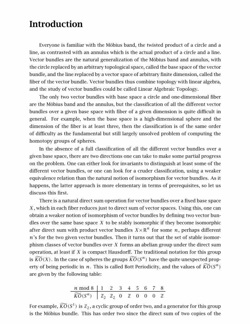
is KO(X) . In the case of spheres the groups KO(Sn) have the quite unexpected prop-
erty of being periodic in n . This is called Bott Periodicity, and the values of KO(Sn)
are given by the following table:
n mod 8 1 2 3 4 5 6 7 8
KO(Sn) Z2 Z2 0 Z 0 0 0 Z
For example, KO(S1) is Z2 , a cyclic group of order two, and a generator for this group
is the Mobius bundle. This has order two since the direct sum of two copies of the
2 Introduction
Mobius bundle is the product S1×R2 , as one can see by embedding two Mobius bands
in a solid torus so that they intersect orthogonally along the common core circle of
both bands, which is also the core circle of the solid torus.
Things become simpler if one passes from real vector spaces to complex vector
spaces. The complex version of KO(X) , called K(X) , is constructed in the same way
as KO(X) but using vector bundles whose fibers are vector spaces over C rather than
R . The complex form of Bott Periodicity asserts simply that K(Sn) is Z for n even
and 0 for n odd, so the period is two rather than eight.
The groups K(X) and KO(X) for varying X share certain formal properties with
the cohomology groups studied in classical algebraic topology. Using a more general
form of Bott periodicity, it is in fact possible to extend the groups K(X) and KO(X)
to a full cohomology theory, families of abelian groups Kn(X) and KOn(X) for n ∈ Z
that are periodic in n of period two and eight, respectively. There is more algebraic
structure here than just the additive group structure, however. Tensor products of
vector spaces give rise to tensor products of vector bundles, which in turn give prod-
uct operations in both real and complex K–theory similar to cup product in ordinary
cohomology. Furthermore, exterior powers of vector spaces give natural operations
within K–theory.
With all this extra structure, K–theory becomes a powerful tool, in some ways
more powerful even than ordinary cohomology. The prime example of this is the very
simple proof, once the basic machinery of complex K–theory has been set up, of the
theorem that there are no finite dimensional division algebras over R in dimensions
other than 1, 2, 4, and 8, the dimensions of the classical examples of the real and
complex numbers, the quaternions, and the Cayley octonions. The same proof shows
also that the only spheres whose tangent bundles are product bundles are S1 , S3 , and
S7 , the unit spheres in the complex numbers, quaternions, and octonions.
Another classical problem that can be solved more easily using K–theory than
ordinary cohomology is to find the maximum number of linearly independent tangent
vector fields on the sphere Sn . In this case complex K–theory is not enough, and the
added subtlety of real K–theory is needed. There is an algebraic construction of the
requisite number of vector fields using Clifford algebras, and the task is to show there
can be no more than this construction provides. Clifford algebras also give a nice
explanation for the mysterious sequence of groups appearing in the real form of Bott
periodicity.
Now let us return to the original classification problem for vector bundles over a
given base space and the question of finding invariants to distinguish different vector
bundles. The first such invariant is orientability, the question of whether all the fibers
can be coherently oriented. For example, the Mobius bundle is not orientable since
as one goes all the way around the base circle, the orientation of the fiber lines is
reversed. This does not happen for the annulus, which is an orientable vector bundle.
Introduction 3
Orientability is measured by the first of a sequence of cohomology classes associ-
ated to a vector bundle, called Stiefel-Whitney classes. The next Stiefel-Whitney class
measures a more refined sort of orientability called a spin structure, and the higher
Stiefel-Whitney classes measure whether the vector bundle looks more and more like
a product vector bundle over succesively higher dimensional subspaces of the base
space. Cohomological invariants of vector bundles such as these with nice general
properties are known as characteristic classes. It turns out that Stiefel-Whitney classes
generate all characteristic classes for ordinary cohomology with Z2 coefficients, but
with Z coefficients there are others, called Pontryagin and Euler classes, the latter
being related to the Euler characteristic. Although characteristic classes do not come
close to distinguishing all the different vector bundles over a given base space, except
in low dimensional cases, they have still proved themselves to be quite useful objects.
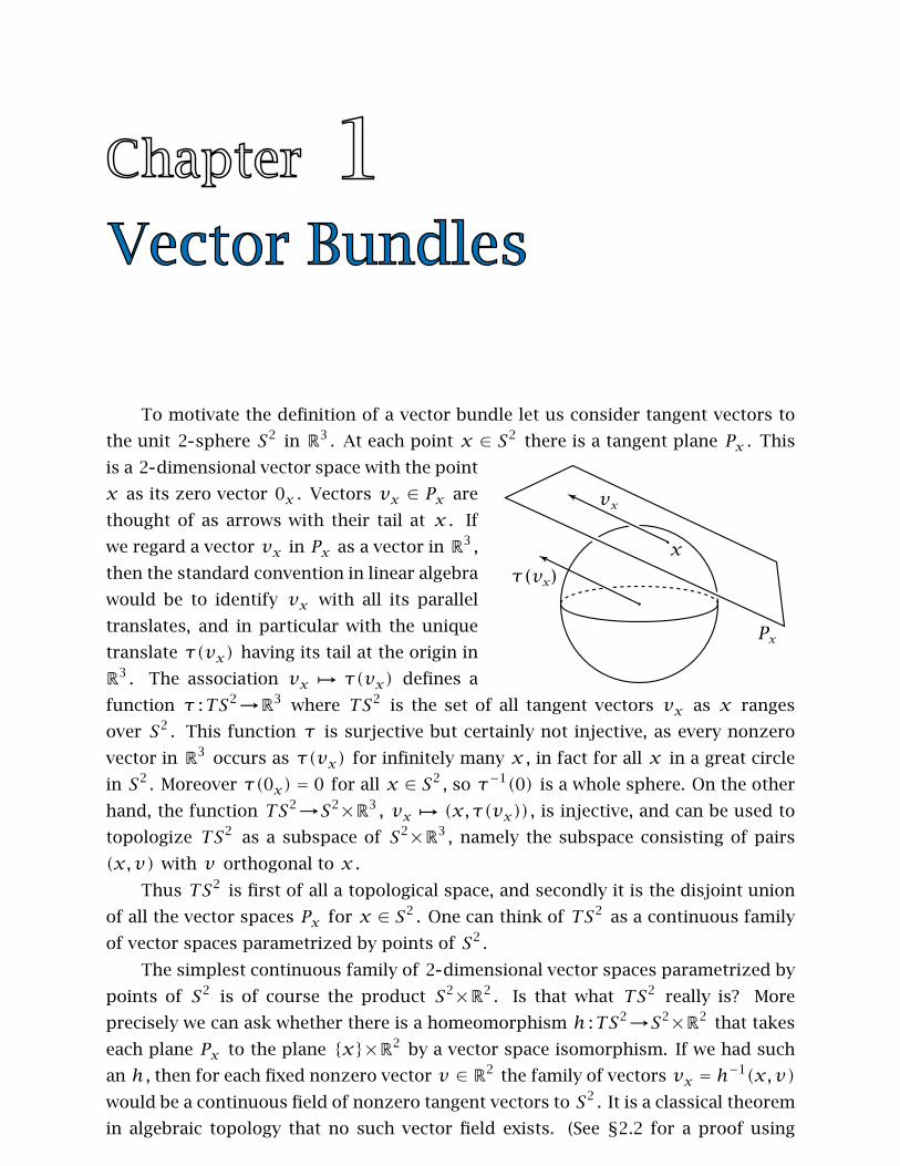
To motivate the definition of a vector bundle let us consider tangent vectors to
the unit 2 sphere S2 in R3 . At each point x ∈ S2 there is a tangent plane Px . This
is a 2 dimensional vector space with the point
x as its zero vector 0x . Vectors vx ∈ Px are
thought of as arrows with their tail at x . If
we regard a vector vx in Px as a vector in R3 ,
then the standard convention in linear algebra
would be to identify vx with all its parallel
translates, and in particular with the unique
translate τ(vx) having its tail at the origin in
R3 . The association vx ֏ τ(vx) defines a
function τ :TS2→R3 where TS2 is the set of all tangent vectors vx as x ranges
over S2 . This function τ is surjective but certainly not injective, as every nonzero
vector in R3 occurs as τ(vx) for infinitely many x , in fact for all x in a great circle
in S2 . Moreover τ(0x) = 0 for all x ∈ S2 , so τ−1(0) is a whole sphere. On the other
hand, the function TS2→S2×R3 , vx֏ (x, τ(vx)) , is injective, and can be used to
topologize TS2 as a subspace of S2×R3 , namely the subspace consisting of pairs
(x,v) with v orthogonal to x .
Thus TS2 is first of all a topological space, and secondly it is the disjoint union
of all the vector spaces Px for x ∈ S2 . One can think of TS2 as a continuous family
of vector spaces parametrized by points of S2 .
The simplest continuous family of 2 dimensional vector spaces parametrized by
points of S2 is of course the product S2×R2 . Is that what TS2 really is? More
precisely we can ask whether there is a homeomorphism h :TS2→S2×R2 that takes
each plane Px to the plane {x}×R2 by a vector space isomorphism. If we had such
an h , then for each fixed nonzero vector v ∈ R2 the family of vectors vx = h−1(x,v)
would be a continuous field of nonzero tangent vectors to S2 . It is a classical theorem
in algebraic topology that no such vector field exists. (See §2.2 for a proof using
Basic Definitions and Constructions Section 1.1 5
techniques from this book.) So TS2 is genuinely twisted, and is not just a disguised
form of the product S2×R2 .
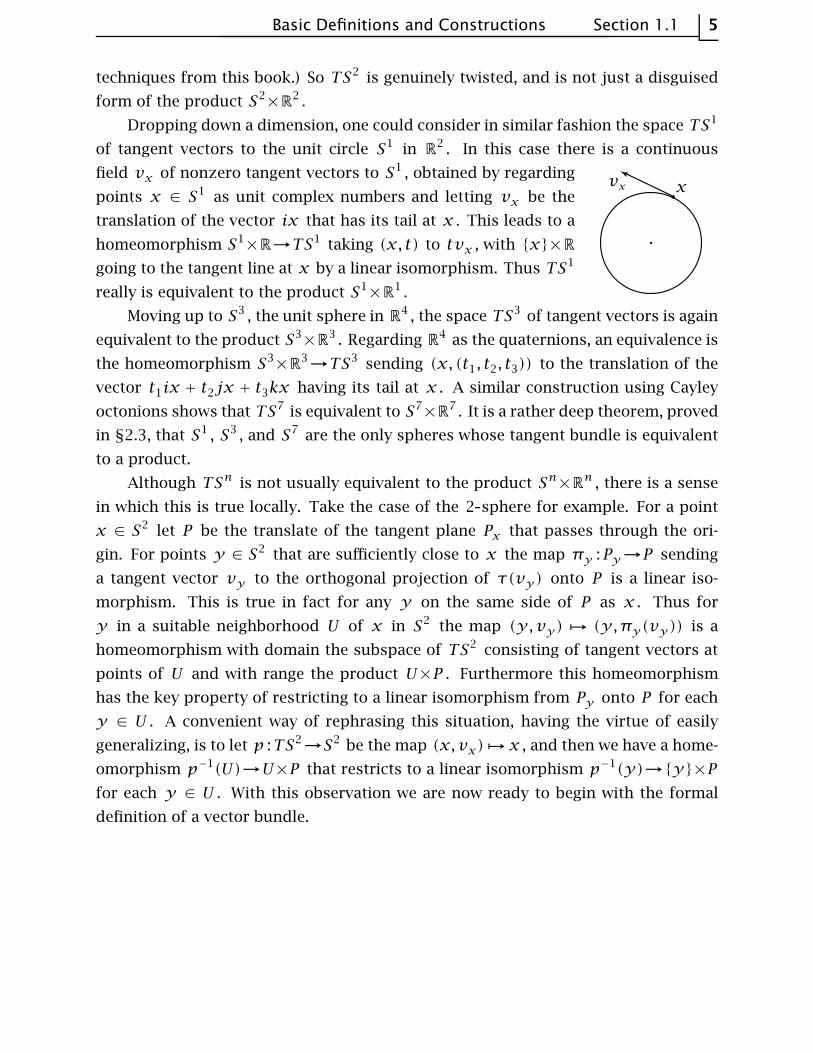
Dropping down a dimension, one could consider in similar fashion the space TS1
of tangent vectors to the unit circle S1 in R2 . In this case there is a continuous
field vx of nonzero tangent vectors to S1 , obtained by regarding
points x ∈ S1 as unit complex numbers and letting vx be the
translation of the vector ix that has its tail at x . This leads to a
homeomorphism S1×R→TS1 taking (x, t) to tvx , with {x}×R
going to the tangent line at x by a linear isomorphism. Thus TS1
really is equivalent to the product S1×R1 .
Moving up to S3 , the unit sphere in R4 , the space TS3 of tangent vectors is again
equivalent to the product S3×R3 . Regarding R4 as the quaternions, an equivalence is
the homeomorphism S3×R3→TS3 sending (x, (t1, t2, t3)) to the translation of the
vector t1ix + t2jx + t3kx having its tail at x . A similar construction using Cayley
octonions shows that TS7 is equivalent to S7×R7 . It is a rather deep theorem, proved
in §2.3, that S1 , S3 , and S7 are the only spheres whose tangent bundle is equivalent
to a product.
Although TSn is not usually equivalent to the product Sn×Rn , there is a sense
in which this is true locally. Take the case of the 2 sphere for example. For a point
x ∈ S2 let P be the translate of the tangent plane Px that passes through the ori-
gin. For points y ∈ S2 that are sufficiently close to x the map πy :Py→P sending
a tangent vector vy to the orthogonal projection of τ(vy) onto P is a linear iso-
morphism. This is true in fact for any y on the same side of P as x . Thus for
y in a suitable neighborhood U of x in S2 the map (y,vy)֏ (y,πy(vy)) is a
homeomorphism with domain the subspace of TS2 consisting of tangent vectors at
points of U and with range the product U×P . Furthermore this homeomorphism
has the key property of restricting to a linear isomorphism from Py onto P for each
y ∈ U . A convenient way of rephrasing this situation, having the virtue of easily
generalizing, is to let p :TS2→S2 be the map (x,vx)֏x , and then we have a home-
omorphism p−1(U)→U×P that restricts to a linear isomorphism p−1(y)→{y}×Pfor each y ∈ U . With this observation we are now ready to begin with the formal
definition of a vector bundle.
6 Chapter 1 Vector Bundles
1.1 Basic Definitions and Constructions
Throughout the book we use the word “map" to mean a continuous function.
An n dimensional vector bundle is a map p :E→B together with a real vector
space structure on p−1(b) for each b ∈ B , such that the following local triviality
condition is satisfied: There is a cover of B by open sets Uα for each of which there
exists a homeomorphism hα :p−1(Uα)→Uα×Rn taking p−1(b) to {b}×Rn by a vec-
tor space isomorphism for each b ∈ Uα . Such an hα is called a local trivialization of
the vector bundle. The space B is called the base space, E is the total space, and the
vector spaces p−1(b) are the fibers. Often one abbreviates terminology by just calling
the vector bundle E , letting the rest of the data be implicit.
We could equally well take C in place of R as the scalar field, obtaining the notion
of a complex vector bundle. We will focus on real vector bundles in this chapter.
Usually the complex case is entirely analogous. In the next chapter complex vector
bundles will play the larger role, however.
Here are some examples of vector bundles:
(1) The product or trivial bundle E = B×Rn with p the projection onto the first
factor.
(2) If we let E be the quotient space of I×R under the identifications (0, t) ∼ (1,−t) ,
then the projection I×R→I induces a map p :E→S1 which is a 1 dimensional vector
bundle, or line bundle. Since E is homeomorphic to a Mobius band with its boundary
circle deleted, we call this bundle the Mobius bundle.
(3) The tangent bundle of the unit sphere Sn in Rn+1 , a vector bundle p :E→Sn
where E = { (x,v) ∈ Sn×Rn+1 | x ⊥ v } and we think of v as a tangent vector to
Sn by translating it so that its tail is at the head of x , on Sn . The map p :E→Sn
sends (x,v) to x . To construct local trivializations, choose any point x ∈ Sn and
let Ux ⊂ Sn be the open hemisphere containing x and bounded by the hyperplane
through the origin orthogonal to x . Define hx :p−1(Ux)→Ux×p−1(x) ≈ Ux×Rn
by hx(y,v) = (y,πx(v)) where πx is orthogonal projection onto the hyperplane
p−1(x) . Then hx is a local trivialization since πx restricts to an isomorphism of
p−1(y) onto p−1(x) for each y ∈ Ux .
(4) The normal bundle to Sn in Rn+1 , a line bundle p :E→Sn with E consisting of
pairs (x,v) ∈ Sn×Rn+1 such that v is perpendicular to the tangent plane to Sn at
x , or in other words, v = tx for some t ∈ R . The map p :E→Sn is again given by
p(x,v) = x . As in the previous example, local trivializations hx :p−1(Ux)→Ux×Rcan be obtained by orthogonal projection of the fibers p−1(y) onto p−1(x) for y ∈
Ux .
(5) Real projective n space RPn is the space of lines in Rn+1 through the origin.
Since each such line intersects the unit sphere Sn in a pair of antipodal points, we can
Basic Definitions and Constructions Section 1.1 7
also regard RPn as the quotient space of Sn in which antipodal pairs of points are
identified. The canonical line bundle p :E→RPn has as its total space E the subspace
of RPn×Rn+1 consisting of pairs (ℓ, v) with v ∈ ℓ , and p(ℓ,v) = ℓ . Again local
trivializations can be defined by orthogonal projection.
There is also an infinite-dimensional projective space RP∞ which is the union
of the finite-dimensional projective spaces RPn under the inclusions RPn ⊂ RPn+1
coming from the natural inclusions Rn+1 ⊂ Rn+2 . The topology we use on RP∞ is
the weak or direct limit topology, for which a set in RP∞ is open iff it intersects each
RPn in an open set. The inclusions RPn ⊂ RPn+1 induce corresponding inclusions
of canonical line bundles, and the union of all these is a canonical line bundle over
RP∞ , again with the direct limit topology. Local trivializations work just as in the
finite-dimensional case.
(6) The canonical line bundle over RPn has an orthogonal complement, the space
E⊥ = { (ℓ, v) ∈ RPn×Rn+1 | v ⊥ ℓ } . The projection p :E⊥→RPn , p(ℓ,v) = ℓ ,
is a vector bundle with fibers the orthogonal subspaces ℓ⊥ , of dimension n . Local
trivializations can be obtained once more by orthogonal projection.
A natural generalization of RPn is the so-called Grassmann manifold Gk(Rn) ,
the space of all k dimensional planes through the origin in Rn . The topology on this
space will be defined precisely in §1.2, along with a canonical k dimensional vector
bundle over it consisting of pairs (ℓ, v) where ℓ is a point in Gk(Rn) and v is a
vector in ℓ . This too has an orthogonal complement, an (n− k) dimensional vector
bundle consisting of pairs (ℓ, v) with v orthogonal to ℓ .
An isomorphism between vector bundles p1 :E1→B and p2 :E2→B over the same
base space B is a homeomorphism h :E1→E2 taking each fiber p−11 (b) to the cor-
responding fiber p−12 (b) by a linear isomorphism. Thus an isomorphism preserves
all the structure of a vector bundle, so isomorphic bundles are often regarded as the
same. We use the notation E1 ≈ E2 to indicate that E1 and E2 are isomorphic.
For example, the normal bundle of Sn in Rn+1 is isomorphic to the product bun-
dle Sn×R by the map (x, tx)֏ (x, t) . The tangent bundle to S1 is also isomorphic
to the trivial bundle S1×R , via (eiθ , iteiθ)֏ (eiθ , t) , for eiθ ∈ S1 and t ∈ R .
As a further example, the Mobius bundle in (2) above is isomorphic to the canon-
ical line bundle over RP1 ≈ S1 . Namely, RP1 is swept out by a line rotating through
an angle of π , so the vectors in these lines sweep out a rectangle [0, π]×R with the
two ends {0}×R and {π}×R identified. The identification is (0, x) ∼ (π,−x) since
rotating a vector through an angle of π produces its negative.
Sections
A section of a vector bundle p :E→B is a map s :B→E assigning to each b ∈ B a
vector s(b) in the fiber p−1(b) . The condition s(b) ∈ p−1(b) can also be written as
8 Chapter 1 Vector Bundles
ps = 11, the identity map of B . Every vector bundle has a canonical section, the zero
section whose value is the zero vector in each fiber. We often identify the zero section
with its image, a subspace of E which projects homeomorphically onto B by p .
One can sometimes distinguish nonisomorphic bundles by looking at the com-
plement of the zero section since any vector bundle isomorphism h :E1→E2 must
take the zero section of E1 onto the zero section of E2 , so the complements of the
zero sections in E1 and E2 must be homeomorphic. For example, we can see that the
Mobius bundle is not isomorphic to the product bundle S1×R since the complement
of the zero section is connected for the Mobius bundle but not for the product bundle.
At the other extreme from the zero section would be a section whose values are
all nonzero. Not all vector bundles have such a section. Consider for example the
tangent bundle to Sn . Here a section is just a tangent vector field to Sn . As we shall
show in §2.2, Sn has a nonvanishing vector field iff n is odd. From this it follows
that the tangent bundle of Sn is not isomorphic to the trivial bundle if n is even
and nonzero, since the trivial bundle obviously has a nonvanishing section, and an
isomorphism between vector bundles takes nonvanishing sections to nonvanishing
sections.
In fact, an n dimensional bundle p :E→B is isomorphic to the trivial bundle iff
it has n sections s1, · · · , sn such that the vectors s1(b), · · · , sn(b) are linearly inde-
pendent in each fiber p−1(b) . In one direction this is evident since the trivial bundle
certainly has such sections and an isomorphism of vector bundles takes linearly inde-
pendent sections to linearly independent sections. Conversely, if one has n linearly
independent sections si , the map h :B×Rn→E given by h(b, t1, · · · , tn) =∑i tisi(b)
is a linear isomorphism in each fiber, and is continuous since its composition with
a local trivialization p−1(U)→U×Rn is continuous. Hence h is an isomorphism by
the following useful technical result:
Lemma 1.1. A continuous map h :E1→E2 between vector bundles over the same
base space B is an isomorphism if it takes each fiber p−11 (b) to the corresponding
fiber p−12 (b) by a linear isomorphism.
Proof: The hypothesis implies that h is one-to-one and onto. What must be checked is
that h−1 is continuous. This is a local question, so we may restrict to an open set U ⊂ B
over which E1 and E2 are trivial. Composing with local trivializations reduces to the
case that h is a continuous map U×Rn→U×Rn of the form h(x,v) = (x,gx(v)) .
Here gx is an element of the group GLn(R) of invertible linear transformations of
Rn , and gx depends continuously on x . This means that if gx is regarded as an
n×n matrix, its n2 entries depend continuously on x . The inverse matrix g−1x also
depends continuously on x since its entries can be expressed algebraically in terms
of the entries of gx , namely, g−1x is 1/(detgx) times the classical adjoint matrix of
gx . Therefore h−1(x,v) = (x,g−1x (v)) is continuous. ⊔⊓
Basic Definitions and Constructions Section 1.1 9
As an example, the tangent bundle to S1 is trivial because it has the section
(x1, x2)֏ (−x2, x1) for (x1, x2) ∈ S1 . In terms of complex numbers, if we set
z = x1 + ix2 then this section is z֏ iz since iz = −x2 + ix1 .
There is an analogous construction using quaternions instead of complex num-
bers. Quaternions have the form z = x1+ix2+jx3+kx4 , and form a division algebra
H via the multiplication rules i2 = j2 = k2 = −1, ij = k , jk = i , ki = j , ji = −k ,
kj = −i , and ik = −j . If we identify H with R4 via the coordinates (x1, x2, x3, x4) ,
then the unit sphere is S3 and we can define three sections of its tangent bundle by
the formulas
z֏ iz or (x1, x2, x3, x4)֏ (−x2, x1,−x4, x3)
z֏ jz or (x1, x2, x3, x4)֏ (−x3, x4, x1,−x2)
z֏ kz or (x1, x2, x3, x4)֏ (−x4,−x3, x2, x1)
It is easy to check that the three vectors in the last column are orthogonal to each other
and to (x1, x2, x3, x4) , so we have three linearly independent nonvanishing tangent
vector fields on S3 , and hence the tangent bundle to S3 is trivial.
The underlying reason why this works is that quaternion multiplication satisfies
|zw| = |z||w| , where |·| is the usual norm of vectors in R4 . Thus multiplication by a
quaternion in the unit sphere S3 is an isometry of H . The quaternions 1, i, j, k form
the standard orthonormal basis for R4 , so when we multiply them by an arbitrary unit
quaternion z ∈ S3 we get a new orthonormal basis z, iz, jz, kz .
The same constructions work for the Cayley octonions, a division algebra struc-
ture on R8 . Thinking of R8 as H×H , multiplication of octonions is defined by
(z1, z2)(w1,w2) = (z1w1−w2z2, z2w1+w2z1) and satisfies the key property |zw| =
|z||w| . This leads to the construction of seven orthogonal tangent vector fields on
the unit sphere S7 , so the tangent bundle to S7 is also trivial. As we shall show in
§2.3, the only spheres with trivial tangent bundle are S1 , S3 , and S7 .
Another way of characterizing the trivial bundle E ≈ B×Rn is to say that there is a
continuous projection map E→Rn which is a linear isomorphism on each fiber, since
such a projection together with the bundle projection E→B gives an isomorphism
E ≈ B×Rn , by Lemma 1.1.
Direct Sums
Given two vector bundles p1 :E1→B and p2 :E2→B over the same base space B ,
we would like to create a third vector bundle over B whose fiber over each point of B
is the direct sum of the fibers of E1 and E2 over this point. This leads us to define
the direct sum of E1 and E2 as the space
E1⊕E2 = { (v1, v2) ∈ E1×E2 | p1(v1) = p2(v2) }
There is then a projection E1⊕E2→B sending (v1, v2) to the point p1(v1) = p2(v2) .
The fibers of this projection are the direct sums of the fibers of E1 and E2 , as we
10 Chapter 1 Vector Bundles
wanted. For a relatively painless verification of the local triviality condition we make
two preliminary observations:
(a) Given a vector bundle p :E→B and a subspace A ⊂ B , then p :p−1(A)→A is
clearly a vector bundle. We call this the restriction of E over A .
(b) Given vector bundles p1 :E1→B1 and p2 :E2→B2 , then p1×p2 :E1×E2→B1×B2
is also a vector bundle, with fibers the products p−11 (b1)×p
−12 (b2) . For if we have
local trivializations hα :p−11 (Uα)→Uα×Rn and hβ :p−1
2 (Uβ)→Uβ×Rm for E1 and
E2 , then hα×hβ is a local trivialization for E1×E2 .
Then if E1 and E2 both have the same base space B , the restriction of the product
E1×E2 over the diagonal B = {(b, b) ∈ B×B} is exactly E1⊕E2 .
The direct sum of two trivial bundles is again a trivial bundle, clearly, but the
direct sum of nontrivial bundles can also be trivial. For example, the direct sum of
the tangent and normal bundles to Sn in Rn+1 is the trivial bundle Sn×Rn+1 since
elements of the direct sum are triples (x,v, tx) ∈ Sn×Rn+1×Rn+1 with x ⊥ v , and
the map (x,v, tx)֏(x,v+tx) gives an isomorphism of the direct sum bundle with
Sn×Rn+1 . So the tangent bundle to Sn is stably trivial : it becomes trivial after taking
the direct sum with a trivial bundle.
As another example, the direct sum E⊕E⊥ of the canonical line bundle E→RPn
with its orthogonal complement, defined in example (6) above, is isomorphic to the
trivial bundle RPn×Rn+1 via the map (ℓ, v,w)֏ (ℓ, v +w) for v ∈ ℓ and w ⊥ ℓ .
Specializing to the case n = 1, the bundle E⊥ is isomorphic to E itself by the map that
rotates each vector in the plane by 90 degrees. We noted earlier that E is isomorphic
to the Mobius bundle over S1 = RP1 , so it follows that the direct sum of the Mobius
bundle with itself is the trivial bundle. To see this geometrically, embed the Mobius
bundle in the product bundle S1×R2 by taking the line in the fiber {θ}×R2 that makes
an angle of θ/2 with the x axis, and then the orthogonal lines in the fibers form a
second copy of the Mobius bundle, giving a decomposition of the product S1×R2 as
the direct sum of two Mobius bundles.
Example: The tangent bundle of real projective space. Starting with the isomor-
phism Sn×Rn+1 ≈ TSn⊕NSn , where NSn is the normal bundle of Sn in Rn+1 ,
suppose we factor out by the identifications (x,v) ∼ (−x,−v) on both sides of this
isomorphism. Applied to TSn this identification yields TRPn , the tangent bundle to
RPn . This is saying that a tangent vector to RPn is equivalent to a pair of antipodal
tangent vectors to Sn . A moment’s reflection shows this to be entirely reasonable,
although a formal proof would require a significant digression on what precisely tan-
gent vectors to a smooth manifold are, a digression we shall skip here. What we will
show is that even though the direct sum of TRPn with a trivial line bundle may not
be trivial as it is for a sphere, it does split in an interesting way as a direct sum of
nontrivial line bundles.
Basic Definitions and Constructions Section 1.1 11
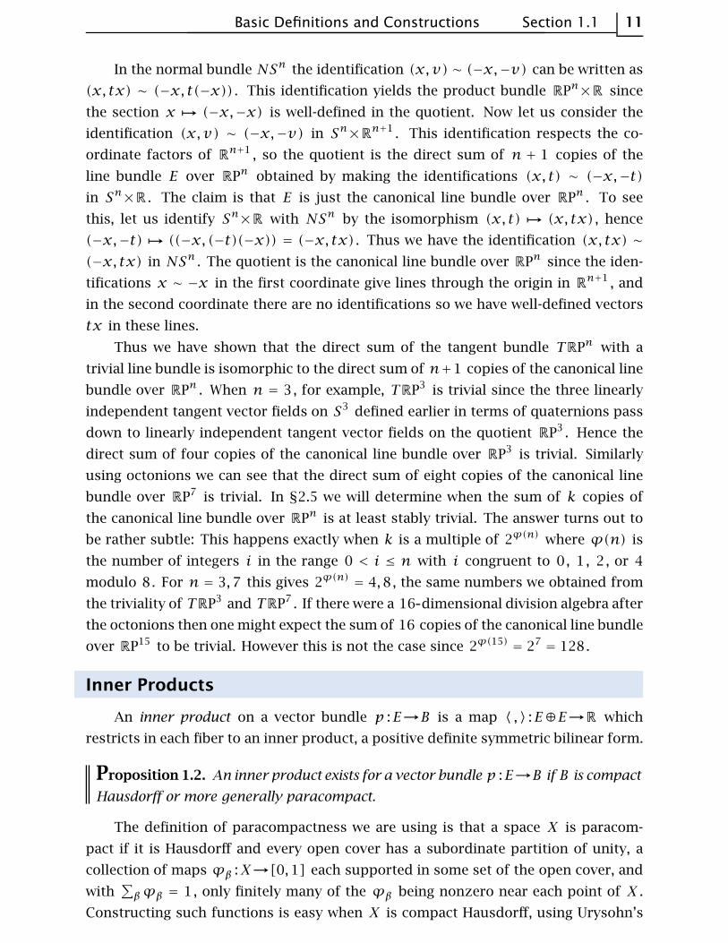
In the normal bundle NSn the identification (x,v) ∼ (−x,−v) can be written as
(x, tx) ∼ (−x, t(−x)) . This identification yields the product bundle RPn×R since
the section x֏ (−x,−x) is well-defined in the quotient. Now let us consider the
identification (x,v) ∼ (−x,−v) in Sn×Rn+1 . This identification respects the co-
ordinate factors of Rn+1 , so the quotient is the direct sum of n + 1 copies of the
line bundle E over RPn obtained by making the identifications (x, t) ∼ (−x,−t)
in Sn×R . The claim is that E is just the canonical line bundle over RPn . To see
this, let us identify Sn×R with NSn by the isomorphism (x, t)֏ (x, tx) , hence
(−x,−t)֏ ((−x, (−t)(−x)) = (−x, tx) . Thus we have the identification (x, tx) ∼
(−x, tx) in NSn . The quotient is the canonical line bundle over RPn since the iden-
tifications x ∼ −x in the first coordinate give lines through the origin in Rn+1 , and
in the second coordinate there are no identifications so we have well-defined vectors
tx in these lines.
Thus we have shown that the direct sum of the tangent bundle TRPn with a
trivial line bundle is isomorphic to the direct sum of n+1 copies of the canonical line
bundle over RPn . When n = 3, for example, TRP3 is trivial since the three linearly
independent tangent vector fields on S3 defined earlier in terms of quaternions pass
down to linearly independent tangent vector fields on the quotient RP3 . Hence the
direct sum of four copies of the canonical line bundle over RP3 is trivial. Similarly
using octonions we can see that the direct sum of eight copies of the canonical line
bundle over RP7 is trivial. In §2.5 we will determine when the sum of k copies of
the canonical line bundle over RPn is at least stably trivial. The answer turns out to
be rather subtle: This happens exactly when k is a multiple of 2ϕ(n) where ϕ(n) is
the number of integers i in the range 0 < i ≤ n with i congruent to 0, 1, 2, or 4
modulo 8. For n = 3,7 this gives 2ϕ(n) = 4,8, the same numbers we obtained from
the triviality of TRP3 and TRP7 . If there were a 16 dimensional division algebra after
the octonions then one might expect the sum of 16 copies of the canonical line bundle
over RP15 to be trivial. However this is not the case since 2ϕ(15) = 27 = 128.
Inner Products
An inner product on a vector bundle p :E→B is a map 〈 , 〉 :E⊕E→R which
restricts in each fiber to an inner product, a positive definite symmetric bilinear form.
Proposition 1.2. An inner product exists for a vector bundle p :E→B if B is compact
Hausdorff or more generally paracompact.
The definition of paracompactness we are using is that a space X is paracom-
pact if it is Hausdorff and every open cover has a subordinate partition of unity, a
collection of maps ϕβ :X→[0,1] each supported in some set of the open cover, and
with∑βϕβ = 1, only finitely many of the ϕβ being nonzero near each point of X .
Constructing such functions is easy when X is compact Hausdorff, using Urysohn’s
12 Chapter 1 Vector Bundles
Lemma. This is done in the appendix to this chapter, where we also show that certain
classes of noncompact spaces are paracompact. Most spaces that arise naturally in
algebraic topology are paracompact.
Proof: An inner product for p :E→B can be constructed by first using local trivial-
izations hα :p−1(Uα)→Uα×Rn , to pull back the standard inner product in Rn to an
inner product 〈·, ·〉α on p−1(Uα) , then setting 〈v,w〉 =∑βϕβp(v)〈v,w〉α(β) where
{ϕβ} is a partition of unity with the support of ϕβ contained in Uα(β) . ⊔⊓
In the case of complex vector bundles one can construct Hermitian inner products
in the same way.
In linear algebra one can show that a vector subspace is always a direct summand
by taking its orthogonal complement. We will show now that the corresponding result
holds for vector bundles over a paracompact base. A vector subbundle of a vector
bundle p :E→B has the natural definition: a subspace E0 ⊂ E intersecting each fiber
of E in a vector subspace, such that the restriction p :E0→B is a vector bundle.
Proposition 1.3. If E→B is a vector bundle over a paracompact base B and E0 ⊂ E
is a vector subbundle, then there is a vector subbundle E⊥0 ⊂ E such that E0⊕E⊥0 ≈ E .
Proof: With respect to a chosen inner product on E , let E⊥0 be the subspace of E
which in each fiber consists of all vectors orthogonal to vectors in E0 . We claim
that the natural projection E⊥0→B is a vector bundle. If this is so, then E0⊕E⊥0 is
isomorphic to E via the map (v,w)֏ v +w , using Lemma 1.1.
To see that E⊥0 satisfies the local triviality condition for a vector bundle, note
first that we may assume E is the product B×Rn since the question is local in B .
Since E0 is a vector bundle, of dimension m say, it has m independent local sections
b֏ (b, si(b)) near each point b0 ∈ B . We may enlarge this set of m independent
local sections of E0 to a set of n independent local sections b֏ (b, si(b)) of E by
choosing sm+1, · · · , sn first in the fiber p−1(b0) , then taking the same vectors for
all nearby fibers, since if s1, · · · , sm, sm+1, · · · , sn are independent at b0 , they will
remain independent for nearby b by continuity of the determinant function. Apply
the Gram-Schmidt orthogonalization process to s1, · · · , sm, sm+1, · · · , sn in each fiber,
using the given inner product, to obtain new sections s′i . The explicit formulas for
the Gram-Schmidt process show the s′i ’s are continuous, and the first m of them are
a basis for E0 in each fiber. The sections s′i allow us to define a local trivialization
h :p−1(U)→U×Rn with h(b, s′i(b)) equal to the ith standard basis vector of Rn .
This h carries E0 to U×Rm and E⊥0 to U×Rn−m , so h||E⊥0 is a local trivialization of
E⊥0 . ⊔⊓
Note that when the subbundle E0 is equal to E itself, the last part of the proof
shows that for any vector bundle with an inner product it is always possible to choose

Basic Definitions and Constructions Section 1.1 13
local trivializations that carry the inner product to the standard inner product, so the
local trivializations are by isometries.
We have seen several cases where the sum of two bundles, one or both of which
may be nontrivial, is the trivial bundle. Here is a general result result along these lines:
Proposition 1.4. For each vector bundle E→B with B compact Hausdorff there
exists a vector bundle E′→B such that E⊕E′ is the trivial bundle.
This can fail when B is noncompact. An example is the canonical line bundle over
RP∞ , as we shall see in Example 3.6.
Proof: To motivate the construction, suppose first that the result holds and hence
that E is a subbundle of a trivial bundle B×RN . Composing the inclusion of E into
this product with the projection of the product onto RN yields a map E→R
N that
is a linear injection on each fiber. Our strategy will be to reverse the logic here, first
constructing a map E→RN that is a linear injection on each fiber, then showing that
this gives an embedding of E in B×RN as a direct summand.
Each point x ∈ B has a neighborhood Ux over which E is trivial. By Urysohn’s
Lemma there is a map ϕx :B→[0,1] that is 0 outside Ux and nonzero at x . Letting
x vary, the sets ϕ−1x (0,1] form an open cover of B . By compactness this has a
finite subcover. Let the corresponding Ux ’s and ϕx ’s be relabeled Ui and ϕi . Define
gi :E→Rn by gi(v) =ϕi
(p(v)
)(πihi(v)
)where p is the projection E→B and πihi
is the composition of a local trivialization hi :p−1(Ui)→Ui×Rn with the projection
πi to Rn . Then gi is a linear injection on each fiber over ϕ−1i (0,1] , so if we make
the various gi ’s the coordinates of a map g :E→RN with RN a product of copies of
Rn , then g is a linear injection on each fiber.
The map g is the second coordinate of a map f :E→B×RN with first coordinate
p . The image of f is a subbundle of the product B×RN since projection of RN onto
the ith Rn factor gives the second coordinate of a local trivialization over ϕ−1i (0,1] .
Thus we have E isomorphic to a subbundle of B×RN so by preceding proposition
there is a complementary subbundle E′ with E⊕E′ isomorphic to B×RN . ⊔⊓
Tensor Products
In addition to direct sum, a number of other algebraic constructions with vec-
tor spaces can be extended to vector bundles. One which is particularly important
for K–theory is tensor product. For vector bundles p1 :E1→B and p2 :E2→B , let
E1⊗E2 , as a set, be the disjoint union of the vector spaces p−11 (x)⊗p
−12 (x) for
x ∈ B . The topology on this set is defined in the following way. Choose isomor-
phisms hi :p−1i (U)→U×Rni for each open set U ⊂ B over which E1 and E2 are
trivial. Then a topology TU on the set p−11 (U)⊗p
−12 (U) is defined by letting the
14 Chapter 1 Vector Bundles
fiberwise tensor product map h1 ⊗h2 :p−11 (U)⊗p
−12 (U)→U×(Rn1⊗Rn2) be a home-
omorphism. The topology TU is independent of the choice of the hi ’s since any
other choices are obtained by composing with isomorphisms of U×Rni of the form
(x,v)֏(x,gi(x)(v)) for continuous maps gi :U→GLni(R) , hence h1 ⊗h2 changes
by composing with analogous isomorphisms of U×(Rn1⊗Rn2) whose second coordi-
nates g1 ⊗g2 are continuous maps U→GLn1n2(R) , since the entries of the matrices
g1(x)⊗g2(x) are the products of the entries of g1(x) and g2(x) . When we replace
U by an open subset V , the topology on p−11 (V)⊗p
−12 (V) induced by TU is the same
as the topology TV since local trivializations over U restrict to local trivializations
over V . Hence we get a well-defined topology on E1⊗E2 making it a vector bundle
over B .
There is another way to look at this construction that takes as its point of depar-
ture a general method for constructing vector bundles we have not mentioned previ-
ously. If we are given a vector bundle p :E→B and an open cover {Uα} of B with lo-
cal trivializations hα :p−1(Uα)→Uα×Rn , then we can reconstruct E as the quotient
space of the disjoint union∐α(Uα×R
n) obtained by identifying (x,v) ∈ Uα×Rn
with hβh−1α (x,v) ∈ Uβ×R
n whenever x ∈ Uα ∩ Uβ . The functions hβh−1α can
be viewed as maps gβα :Uα ∩ Uβ→GLn(R) . These satisfy the ‘cocycle condition’
gγβgβα = gγα on Uα ∩ Uβ ∩ Uγ . Any collection of ‘gluing functions’ gβα satisfying
this condition can be used to construct a vector bundle E→B .
In the case of tensor products, suppose we have two vector bundles E1→B and
E2→B . We can choose an open cover {Uα} with both E1 and E2 trivial over each Uα ,
and so obtain gluing functions giβα :Uα ∩Uβ→GLni(R) for each Ei . Then the gluing
functions for the bundle E1⊗E2 are the tensor product functions g1βα ⊗g
2βα assigning
to each x ∈ Uα ∩Uβ the tensor product of the two matrices g1βα(x) and g2
βα(x) .
It is routine to verify that the tensor product operation for vector bundles over a
fixed base space is commutative, associative, and has an identity element, the trivial
line bundle. It is also distributive with respect to direct sum.
If we restrict attention to line bundles, then the set Vect1(B) of isomorphism
classes of one-dimensional vector bundles over B is an abelian group with respect
to the tensor product operation. The inverse of a line bundle E→B is obtained by
replacing its gluing matrices gβα(x) ∈ GL1(R) with their inverses. The cocycle con-
dition is preserved since 1×1 matrices commute. If we give E an inner product, we
may rescale local trivializations hα to be isometries, taking vectors in fibers of E to
vectors in R1 of the same length. Then all the values of the gluing functions gβα are
±1, being isometries of R . The gluing functions for E⊗E are the squares of these
gβα ’s, hence are identically 1, so E⊗E is the trivial line bundle. Thus each element of
Vect1(B) is its own inverse. As we shall see in §3.1, the group Vect1(B) is isomorphic
to a standard object in algebraic topology, the cohomology group H1(B;Z2) when B
is homotopy equivalent to a CW complex.
Basic Definitions and Constructions Section 1.1 15
These tensor product constructions work equally well for complex vector bundles.
Tensor product again makes the complex analog Vect1C(B) of Vect1(B) into an abelian
group, but after rescaling the gluing functions gβα for a complex line bundle E , the
values are complex numbers of norm 1, not necessarily ±1, so we cannot expect E⊗E
to be trivial. In §3.1 we will show that the group Vect1C(B) is isomorphic to H2(B;Z)
when B is homotopy equivalent to a CW complex.
We may as well mention here another general construction for complex vector
bundles E→B , the notion of the conjugate bundle E→B . As a topological space, E
is the same as E , but the vector space structure in the fibers is modified by redefining
scalar multiplication by the rule λ(v) = λv where the right side of this equation
means scalar multiplication in E and the left side means scalar multiplication in E .
This implies that local trivializations for E are obtained from local trivializations for
E by composing with the coordinatewise conjugation map Cn→Cn in each fiber. The
effect on the gluing maps gβα is to replace them by their complex conjugates as
well. Specializing to line bundles, we then have E⊗E isomorphic to the trivial line
bundle since its gluing maps have values zz = 1 for z a unit complex number. Thus
conjugate bundles provide inverses in Vect1C(B) .
Besides tensor product of vector bundles, another construction useful in K–theory
is the exterior power λk(E) of a vector bundle E . Recall from linear algebra that
the exterior power λk(V) of a vector space V is the quotient of the k fold tensor
product V ⊗ · · · ⊗V by the subspace generated by vectors of the form v1 ⊗ · · · ⊗vk−
sgn(σ)vσ(1) ⊗ · · · ⊗vσ(k) where σ is a permutation of the subscripts and sgn(σ) =
±1 is its sign, +1 for an even permutation and −1 for an odd permutation. If V has
dimension n then λk(V) has dimension(nk
). Now to define λk(E) for a vector bundle
p :E→B the procedure follows closely what we did for tensor product. We first form
the disjoint union of the exterior powers λk(p−1(x)) of all the fibers p−1(x) , then we
define a topology on this set via local trivializations. The key fact about tensor product
which we needed before was that the tensor product ϕ⊗ψ of linear transformations
ϕ and ψ depends continuously on ϕ and ψ . For exterior powers the analogous fact
is that a linear map ϕ :Rn→Rn induces a linear map λk(ϕ) :λk(Rn)→λk(Rn) which
depends continuously on ϕ . This holds since λk(ϕ) is a quotient map of the k fold
tensor product of ϕ with itself.
Associated Fiber Bundles
If we modify the definition of a vector bundle by dropping all references to vector
spaces and replace the model fiber Rn by an arbitrary space F , then we have the more
general notion of a fiber bundle with fiber F . This is a map p :E→B such that there
is a cover of B by open sets Uα for each of which there exists a homeomorphism
hα :p−1(Uα)→Uα×F taking p−1(b) to {b}×F for each b ∈ Uα . We will describe
now several different ways of constructing fiber bundles from vector bundles.
16 Chapter 1 Vector Bundles
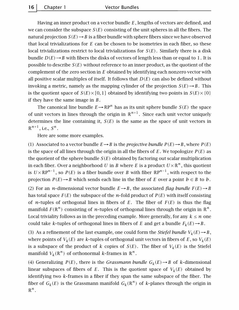
Having an inner product on a vector bundle E , lengths of vectors are defined, and
we can consider the subspace S(E) consisting of the unit spheres in all the fibers. The
natural projection S(E)→B is a fiber bundle with sphere fibers since we have observed
that local trivializations for E can be chosen to be isometries in each fiber, so these
local trivializations restrict to local trivializations for S(E) . Similarly there is a disk
bundle D(E)→B with fibers the disks of vectors of length less than or equal to 1. It is
possible to describe S(E) without reference to an inner product, as the quotient of the
complement of the zero section in E obtained by identifying each nonzero vector with
all positive scalar multiples of itself. It follows that D(E) can also be defined without
invoking a metric, namely as the mapping cylinder of the projection S(E)→B . This
is the quotient space of S(E)×[0,1] obtained by identifying two points in S(E)×{0}
if they have the same image in B .
The canonical line bundle E→RPn has as its unit sphere bundle S(E) the space
of unit vectors in lines through the origin in Rn+1 . Since each unit vector uniquely
determines the line containing it, S(E) is the same as the space of unit vectors in
Rn+1 , i.e., Sn .
Here are some more examples.
(1) Associated to a vector bundle E→B is the projective bundle P(E)→B , where P(E)
is the space of all lines through the origin in all the fibers of E . We topologize P(E) as
the quotient of the sphere bundle S(E) obtained by factoring out scalar multiplication
in each fiber. Over a neighborhood U in B where E is a product U×Rn , this quotient
is U×RPn−1 , so P(E) is a fiber bundle over B with fiber RPn−1 , with respect to the
projection P(E)→B which sends each line in the fiber of E over a point b ∈ B to b .
(2) For an n dimensional vector bundle E→B , the associated flag bundle F(E)→Bhas total space F(E) the subspace of the n fold product of P(E) with itself consisting
of n tuples of orthogonal lines in fibers of E . The fiber of F(E) is thus the flag
manifold F(Rn) consisting of n tuples of orthogonal lines through the origin in Rn .
Local triviality follows as in the preceding example. More generally, for any k ≤ n one
could take k tuples of orthogonal lines in fibers of E and get a bundle Fk(E)→B .
(3) As a refinement of the last example, one could form the Stiefel bundle Vk(E)→B ,
where points of Vk(E) are k tuples of orthogonal unit vectors in fibers of E , so Vk(E)
is a subspace of the product of k copies of S(E) . The fiber of Vk(E) is the Stiefel
manifold Vk(Rn) of orthonormal k frames in Rn .
(4) Generalizing P(E) , there is the Grassmann bundle Gk(E)→B of k dimensional
linear subspaces of fibers of E . This is the quotient space of Vk(E) obtained by
identifying two k frames in a fiber if they span the same subspace of the fiber. The
fiber of Gk(E) is the Grassmann manifold Gk(Rn) of k planes through the origin in
Rn .
Basic Definitions and Constructions Section 1.1 17
Exercises
1. Show that a vector bundle E→X has k independent sections iff it has a trivial
k dimensional subbundle.
2. For a vector bundle E→X with a subbundle E′ ⊂ E , construct a quotient vector
bundle E/E′→X .
3. Show that the orthogonal complement of a subbundle is independent of the choice
of inner product, up to isomorphism.
18 Chapter 1 Vector Bundles
1.2 Classifying Vector Bundles
As was stated in the Introduction, it is usually a difficult problem to classify all
the different vector bundles over a given base space. The goal of this section will be to
rephrase the problem in terms of a standard concept of algebraic topology, the idea
of homotopy classes of maps. This will allow the problem to be solved directly in a
few very simple cases. Using machinery of algebraic topology, other more difficult
cases can be handled as well, as is explained in §??. The reformulation in terms of
homotopy also offers some conceptual enlightenment about the structure of vector
bundles.
For the reader who is unfamiliar with the notion of homotopy we give the basic
definitions in the Glossary [not yet written], and more details can be found in the
introductory chapter of the author’s book Algebraic Topology.
Pullback Bundles
We will denote the set of isomorphism classes of n dimensional real vector bun-
dles over B by Vectn(B) . The complex analogue, when we need it, will be denoted
by VectnC(B) . Our first task is to show how a map f :A→B gives rise to a function
f∗ : Vect(B)→Vect(A) , in the reverse direction.
Proposition 1.5. Given a map f :A→B and a vector bundle p :E→B , then there
exists a vector bundle p′ :E′→A with a map f ′ :E′→E taking the fiber of E′ over
each point a ∈ A isomorphically onto the fiber of E over f(a) , and such a vector
bundle E′ is unique up to isomorphism.
From the uniqueness statement it follows that the isomorphism type of E′ de-
pends only on the isomorphism type of E since we can compose the map f ′ with
an isomorphism of E with another vector bundle over B . Thus we have a function
f∗ : Vect(B)→Vect(A) taking the isomorphism class of E to the isomorphism class
of E′ . Often the vector bundle E′ is written as f∗(E) and called the bundle induced
by f , or the pullback of E by f .
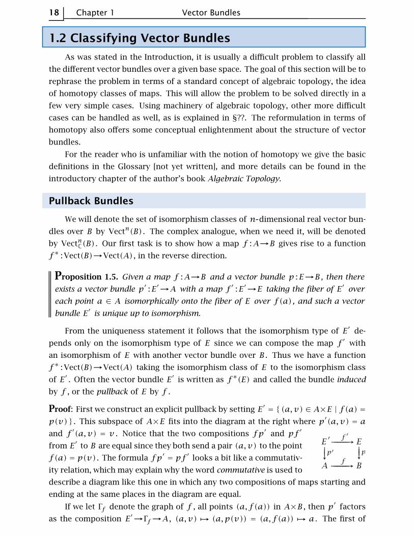
Proof: First we construct an explicit pullback by setting E′ = { (a,v) ∈ A×E | f(a) =
p(v) } . This subspace of A×E fits into the diagram at the right where p′(a,v) = a
and f ′(a,v) = v . Notice that the two compositions fp′ and pf ′
from E′ to B are equal since they both send a pair (a,v) to the point
f(a) = p(v) . The formula fp′ = pf ′ looks a bit like a commutativ-
ity relation, which may explain why the word commutative is used to
describe a diagram like this one in which any two compositions of maps starting and
ending at the same places in the diagram are equal.
If we let Γf denote the graph of f , all points (a, f (a)) in A×B , then p′ factors
as the composition E′→Γf→A , (a,v)֏ (a,p(v)) = (a, f (a))֏ a . The first of
Classifying Vector Bundles Section 1.2 19
these two maps is the restriction of the vector bundle 11×p :A×E→A×B over the
graph Γf , so it is a vector bundle, and the second map is a homeomorphism, so their
composition p′ :E′→A is a vector bundle. The map f ′ obviously takes the fiber E′
over a isomorphically onto the fiber of E over f(a) .
For the uniqueness statement, we can construct an isomorphism from an arbitrary
E′ satisfying the conditions in the proposition to the particular one just constructed by
sending v ′ ∈ E′ to the pair (p′(v ′), f ′(v ′)) . This map obviously takes each fiber of E′
to the corresponding fiber of f∗(E) by a vector space isomorphism, so by Lemma 1.1
it is an isomorphism of vector bundles. ⊔⊓
One can be more explicit about local trivializations in the pullback bundle f∗(E)
constructed above. If E is trivial over a subspace U ⊂ B then f∗(E) is trivial over
f−1(U) since linearly independent sections si of E over U give rise to independent
sections a֏ (a, si(f (a))) of f∗(E) over f−1(U) . In particular, the pullback of a
trivial bundle is a trivial bundle. This can also be seen directly from the definition,
which in the case E = B×Rn just says that f∗(E) consists of the triples (a, b, v) in
A×B×Rn with b = f(a) , so b is redundant and we have just the product A×Rn .
Now let us give some examples of pullbacks.
(1) The restriction of a vector bundle p :E→B over a subspace A ⊂ B can be viewed
as a pullback with respect to the inclusion map AB since the inclusion p−1(A)E
is certainly an isomorphism on each fiber.
(2) Another very special case is when the map f is a constant map, having image a
single point b ∈ B . Then f∗(E) is just the product A×p−1(b) , a trivial bundle.
(3) The tangent bundle TSn is the pullback of the tangent bundle TRPn via the quo-
tient map Sn→RPn . Indeed, TRPn was defined as a quotient space of TSn and the
quotient map takes fibers isomorphically to fibers.
(4) An interesting example which is small enough to be visualized completely is the
pullback of the Mobius bundle E→S1 by the two-to-one map f :S1→S1 given by
f(z) = z2 in complex notation. One can regard the Mobius bundle as the quotient
of S1×R under the identifications (z, t) ∼ (−z,−t) , and the quotient map for this
identification is the map f ′ exhibiting the annulus S1×R as the pullback of the Mobius
bundle. More concretely, the pullback bundle can be thought of as a coat of paint
applied to ‘both sides’ of the Mobius bundle, and the map f ′ sends each molecule
of paint to the point of the Mobius band to which it adheres. Since E has one half-
twist, the pullback has two half-twists, hence is the trivial bundle. More generally, if
En is the pullback of the Mobius bundle by the map z֏ zn , then En is the trivial
bundle for n even and the Mobius bundle for n odd. This can be seen by viewing
the Mobius bundle as the quotient of a strip [0,1]×R obtained by identifying the
two edges {0}×R and {1}×R by a reflection of R , and then the bundle En can be
constructed from n such strips by identifying the right edge of the ith strip to the
20 Chapter 1 Vector Bundles
left edge of the i + 1st strip by a reflection, the number i being taken modulo n so
that the last strip is glued back to the first.
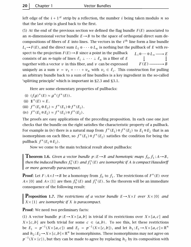
(5) At the end of the previous section we defined the flag bundle F(E) associated to
an n dimensional vector bundle E→B to be the space of orthogonal direct sum de-
compositions of fibers of E into lines. The vectors in the ith line form a line bundle
Li→F(E) , and the direct sum L1⊕ · · ·⊕Ln is nothing but the pullback of E with re-
spect to the projection F(E)→B since a point in the pullback
consists of an n tuple of lines ℓ1 ⊥ · · · ⊥ ℓn in a fiber of E
together with a vector v in this fiber, and v can be expressed
uniquely as a sum v = v1 + · · · + vn with vi ∈ ℓi . This construction for pulling
an arbitrary bundle back to a sum of line bundles is a key ingredient in the so-called
‘splitting principle’ which is important in §2.3 and §3.1.
Here are some elementary properties of pullbacks:
(i) (fg)∗(E) ≈ g∗(f∗(E)) .
(ii) 11∗(E) ≈ E .
(iii) f∗(E1⊕E2) ≈ f∗(E1)⊕f
∗(E2) .
(iv) f∗(E1⊗E2) ≈ f∗(E1)⊗f
∗(E2) .
The proofs are easy applications of the preceding proposition. In each case one just
checks that the bundle on the right satisfies the characteristic property of a pullback.
For example in (iv) there is a natural map from f∗(E1)⊗f∗(E2) to E1⊗E2 that is an
isomorphism on each fiber, so f∗(E1)⊗f∗(E2) satisfies the condition for being the
pullback f∗(E1⊗E2) .
Now we come to the main technical result about pullbacks:
Theorem 1.6. Given a vector bundle p :E→B and homotopic maps f0, f1 :A→B ,
then the induced bundles f∗0 (E) and f∗1 (E) are isomorphic if A is compact Hausdorff
or more generally paracompact.
Proof: Let F :A×I→B be a homotopy from f0 to f1 . The restrictions of F∗(E) over
A×{0} and A×{1} are then f∗0 (E) and f∗1 (E) . So the theorem will be an immediate
consequence of the following result:
Proposition 1.7. The restrictions of a vector bundle E→X×I over X×{0} and
X×{1} are isomorphic if X is paracompact.
Proof: We need two preliminary facts:
(1) A vector bundle p :E→X×[a, b] is trivial if its restrictions over X×[a, c] and
X×[c, b] are both trivial for some c ∈ (a, b) . To see this, let these restrictions
be E1 = p−1(X×[a, c]) and E2 = p−1(X×[c, b]) , and let h1 :E1→X×[a, c]×Rn
and h2 :E2→X×[c, b]×Rn be isomorphisms. These isomorphisms may not agree on
p−1(X×{c}) , but they can be made to agree by replacing h2 by its composition with
Classifying Vector Bundles Section 1.2 21
the isomorphism X×[c, b]×Rn→X×[c, b]×Rn which on each slice X×{x}×Rn is
given by h1h−12 :X×{c}×Rn→X×{c}×Rn . Once h1 and h2 agree on E1 ∩ E2 , they
define a trivialization of E .
(2) For a vector bundle p :E→X×I , there exists an open cover {Uα} of X so that each
restriction p−1(Uα×I)→Uα×I is trivial. This is because for each x ∈ X we can find
open neighborhoods Ux,1, · · · , Ux,k in X and a partition 0 = t0 < t1 < · · · < tk = 1 of
[0,1] such that the bundle is trivial over Ux,i×[ti−1, ti] , using compactness of [0,1] .
Then by (1) the bundle is trivial over Uα×I where Uα = Ux,1 ∩ · · · ∩Ux,k .
Now we prove the proposition. By (2), we can choose an open cover {Uα} of X
so that E is trivial over each Uα×I . Let us first deal with the simpler case that X
is compact Hausdorff. Then a finite number of Uα ’s cover X . Relabel these as Uifor i = 1,2, · · · ,m . As shown in Proposition 1.4 there is a corresponding partition
of unity by functions ϕi with the support of ϕi contained in Ui . For i ≥ 0, let
ψi =ϕ1 + · · · +ϕi , so in particular ψ0 = 0 and ψm = 1. Let Xi be the graph of ψi ,
the subspace of X×I consisting of points of the form (x,ψi(x)) , and let pi :Ei→Xibe the restriction of the bundle E over Xi . Since E is trivial over Ui×I , the natural
projection homeomorphism Xi→Xi−1 lifts to a homeomorphism hi :Ei→Ei−1 which
is the identity outside p−1(Ui×I) and which takes each fiber of Ei isomorphically
onto the corresponding fiber of Ei−1 . Explicitly, on points in p−1(Ui×I) = Ui×I×Rn
we let hi(x,ψi(x), v) = (x,ψi−1(x), v) . The composition h = h1h2 · · ·hm is then
an isomorphism from the restriction of E over X×{1} to the restriction over X×{0} .
In the general case that X is only paracompact, Lemma 1.21 asserts that there is
a countable cover {Vi}i≥1 of X and a partition of unity {ϕi} with ϕi supported in
Vi , such that each Vi is a disjoint union of open sets each contained in some Uα . This
means that E is trivial over each Vi×I . As before we let ψi = ϕ1 + · · · +ϕi and let
pi :Ei→Xi be the restriction of E over the graph of ψi . Also as before we construct
hi :Ei→Ei−1 using the fact that E is trivial over Vi×I . The infinite composition h =
h1h2 · · · is then a well-defined isomorphism from the restriction of E over X×{1}
to the restriction over X×{0} since near each point x ∈ X only finitely many ϕi ’s
are nonzero, so there is a neighborhood of x in which all but finitely many hi ’s are
the identity. ⊔⊓
Corollary 1.8. A homotopy equivalence f :A→B of paracompact spaces induces a
bijection f∗ : Vectn(B)→Vectn(A) . In particular, every vector bundle over a con-
tractible paracompact base is trivial.
Proof: If g is a homotopy inverse of f then we have f∗g∗ = 11∗ = 11 and g∗f∗ =
11∗ = 11. ⊔⊓
We might remark that Theorem 1.6 holds for fiber bundles as well as vector bun-
dles, with the same proof.
22 Chapter 1 Vector Bundles
Clutching Functions
Let us describe a way to construct vector bundles E→Sk with base space a sphere.
Write Sk as the union of its upper and lower hemispheres Dk+ and Dk− , with Dk+∩Dk− =
Sk−1 . Given a map f :Sk−1→GLn(R) , let Ef be the quotient of the disjoint union
Dk+×Rn ∐ Dk−×R
n obtained by identifying (x,v) ∈ ∂Dk−×Rn with (x, f (x)(v)) ∈
∂Dk+×Rn . There is then a natural projection Ef→Sk and this is an n dimensional
vector bundle, as one can most easily see by taking an equivalent definition in which
the two hemispheres of Sk are enlarged slightly to open balls and the identification
occurs over their intersection, a product Sk−1×(−ε, ε) , with the map f used in each
slice Sk−1×{t} . From this viewpoint the construction of Ef is a special case of the
general construction of vector bundles by gluing together products, described earlier
in the discussion of tensor products.
The map f is called a clutching function for Ef , by analogy with the mechanical
clutch which engages and disengages gears in machinery. The same construction
works equally well with C in place of R , so from a map f :Sk−1→GLn(C) one obtains
a complex vector bundle Ef→Sk .
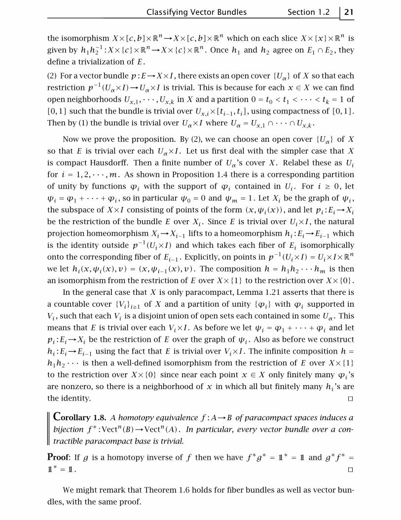
Example 1.9. Let us see how the tangent bundle TS2 to S2 can be described in
these terms. Consider the vector field v+ on D2+ obtained by choosing a tangent
vector at the north pole and transporting this along each
meridian circle in such a way as to maintain a constant
angle with the meridian. By reflecting across the plane
of the equator we obtain a corresponding vector field v−on D2
− . Rotating each vector v+ and v− by 90 degrees
counterclockwise when viewed from outside the sphere,
we obtain vector fields w+ and w− on D2+ and D2
− . The
vector fields v± and w± give trivializations of TS2 over
D2± , allowing us to identify these two halves of TS2 with D2
±×R2 . We can then recon-
struct TS2 as a quotient of the disjoint union of D2+×R
2 and D2−×R
2 by identifying
along S1×R2 using the clutching function f which reads off the coordinates of the
v−,w− vectors in the v+,w+ coordinate system, since the definition of a clutching
function was that it identifies (x,v) ∈ ∂Dk−×Rn with (x, f (x)(v)) ∈ ∂Dk+×R
n . Thus
f rotates (v+,w+) to (v−,w−) . As we go around the equator S1 in the counter-
clockwise direction when viewed from above, starting from a point where the two
trivializations agree, the angle of rotation increases from 0 to 4π . If we parametrize
S1 by the angle θ from the starting point, then f(θ) is rotation by 2θ .
Example 1.10. Let us find a clutching function for the canonical complex line bundle
over CP1 = S2 . The space CP1 is the quotient of C2 − {0} under the equivalence
relation (z0, z1) ∼ λ(z0, z1) for λ ∈ C− {0} . Denote the equivalence class of (z0, z1)
by [z0, z1] . We can also write points of CP1 as ratios z = z0/z1 ∈ C ∪ {∞} = S2 . If
Classifying Vector Bundles Section 1.2 23
we do this, then points in the disk D20 inside the unit circle S1 ⊂ C can be expressed
uniquely in the form [z0/z1,1] = [z,1] with |z| ≤ 1, and points in the disk D2∞
outside S1 can be written uniquely in the form [1, z1/z0] = [1, z−1] with |z−1| ≤ 1.
Over D20 a section of the canonical line bundle is given by [z,1]֏ (z,1) and over
D2∞ a section is [1, z−1]֏ (1, z−1) . These sections determine trivializations of the
canonical line bundle over these two disks, and over their common boundary S1 we
pass from the D2∞ trivialization to the D2
0 trivialization by multiplying by z . Thus if
we take D2∞ as D2
+ and D20 as D2
− then the canonical line bundle has the clutching
function f :S1→GL1(C) defined by f(z) = (z) . If we had taken D2+ to be D2
0 rather
than D2∞ then the clutching function would have been f(z) = (z−1) .
A basic property of the construction of bundles Ef→Sk via clutching functions
f :Sk−1→GLn(R) is that Ef ≈ Eg if f and g are homotopic. For if we have a homo-
topy F :Sk−1×I→GLn(R) from f to g , then the same sort of clutching construction
can be used to produce a vector bundle EF→Sk×I that restricts to Ef over Sk×{0}
and Eg over Sk×{1} . Hence Ef and Eg are isomorphic by Proposition 1.7. Thus if
we denote by [X, Y ] the set of homotopy classes of maps X→Y , then the association
f֏ Ef gives a well-defined map Φ : [Sk−1, GLn(R)] -→Vectn(Sk) .
There is a similarly-defined map Φ for complex vector bundles. This turns out to
have slightly better behavior than in the real case, so we will prove the following basic
result about the complex form of Φ before dealing with the real case.
Proposition 1.11. The map Φ : [Sk−1, GLn(C)]→VectnC(Sk) which sends a clutching
function f to the vector bundle Ef is a bijection.
Proof: We construct an inverse Ψ to Φ . Given an n dimensional vector bundle
p :E→Sk , its restrictions E+ and E− over Dk+ and Dk− are trivial since Dk+ and Dk−are contractible. Choose trivializations h± :E±→Dk±×Cn . Then h+h
−1− defines a map
Sk−1→GLn(C) , whose homotopy class is by definition Ψ(E) ∈ [Sk−1, GLn(C)] . To
see that Ψ(E) is well-defined, note first that any two choices of h± differ by a map
Dk±→GLn(C) . Since Dk± is contractible, such a map is homotopic to a constant map
by composing with a contraction of Dk± . Now we need the fact that GLn(C) is path-
connected. The elementary row operation of modifying a matrix in GLn(C) by adding
a scalar multiple of one row to another row can be realized by a path in GLn(C) , just
by inserting a factor of t in front of the scalar multiple and letting t go from 0 to 1.
By such operations any matrix in GLn(C) can be diagonalized. The set of diagonal
matrices in GLn(C) is path-connected since it is homeomorphic to the product of n
copies of C− {0} .
From this we conclude that h+ and h− are unique up to homotopy. Hence the
composition h+h−1− :Sk−1→GLn(C) is also unique up to homotopy, which means that
Ψ is a well-defined map VectnC(Sk)→[Sk−1, GLn(C)] . It is clear that Ψ and Φ are
inverses of each other. ⊔⊓
24 Chapter 1 Vector Bundles
Example 1.12. Every complex vector bundle over S1 is trivial, since by the proposi-
tion this is equivalent to saying that [S0, GLn(C)] has a single element, or in other
words that GLn(C) is path-connected, which is the case as we saw in the proof of the
proposition.
Example 1.13. Let us show that the canonical line bundle H→CP1 satisfies the rela-
tion (H⊗H)⊕1 ≈ H⊕H where 1 is the trivial one-dimensional bundle. This can be
seen by looking at the clutching functions for these two bundles, which are the maps
S1→GL2(C) given by
z֏
(z2 0
0 1
)and z֏
(z 0
0 z
)
More generally, let us show the formula Efg⊕n ≈ Ef ⊕Eg for n dimensional vec-
tor bundles Ef and Eg over Sk with clutching functions f ,g :Sk−1→GLn(C) , where
fg is the clutching function obtained by pointwise matrix multiplication, fg(x) =
f(x)g(x) .
The bundle Ef⊕Eg has clutching function the map f⊕g :Sk−1→GL2n(C) having
the matrices f(x) in the upper left n×n block and the matrices g(x) in the lower
right n×n block, the other two blocks being zero. Since GL2n(C) is path-connected,
there is a path αt ∈ GL2n(C) from the identity matrix to the matrix of the trans-
formation which interchanges the two factors of Cn×Cn . Then the matrix product
(f ⊕ 11)αt(11⊕ g)αt gives a homotopy from f ⊕ g to fg ⊕ 11, which is the clutching
function for Efg⊕n .
The preceding analysis does not quite work for real vector bundles since GLn(R)
is not path-connected. We can see that there are at least two path-components since
the determinant function is a continuous surjection GLn(R)→R − {0} to a space
with two path-components. In fact GLn(R) has exactly two path-components, as
we will now show. Just as in the complex case we can construct a path from an
arbitrary matrix in GLn(R) to a diagonal matrix. Then by a path of diagonal matrices
we can make all the diagonal entries +1 or −1. Two −1’s represent a 180 degree
rotation of a plane so they can be replaced by +1’s via a path in GLn(R) . This shows
that the subgroup GL+n(R) consisting of matrices of positive determinant is path-
connected. This subgroup has index 2, and GLn(R) is the disjoint union of the two
cosets GL+n(R) and αGL+n(R) for α a fixed matrix of determinant −1. The two cosets
are homeomorphic since the map β֏ αβ is a homeomorphism of GLn(R) with
inverse the map β֏α−1β . Thus both cosets are path-connected and so GLn(R) has
two path-components.
The closest analogy with the complex case is obtained by considering oriented
real vector bundles. Recall from linear algebra that an orientation of a real vector
space is an equivalence class of ordered bases, two ordered bases being equivalent
if the invertible matrix taking the first basis to the second has positive determinant.
Classifying Vector Bundles Section 1.2 25
An orientation of a real vector bundle p :E→B is a function assigning an orientation
to each fiber in such a way that near each point of B there is a local trivialization
h :p−1(U)→U×Rn carrying the orientations of fibers in p−1(U) to the standard ori-
entation of Rn in the fibers of U×Rn . Another way of stating this condition would
be to say that the orientations of fibers of E can be defined by ordered n tuples of
independent local sections. Not all vector bundles can be given an orientation. For
example the Mobius bundle is not orientable. This is because an oriented line bundle
over a paracompact base is always trivial since it has a canonical section formed by
the unit vectors having positive orientation.
Let Vectn+(B) denote the set of isomorphism classes of oriented n dimensional
real vector bundles over B , where isomorphisms are required to preserve orientations.
The clutching construction defines a map Φ : [Sk−1, GL+n(R)] -→Vectn+(Sk) , and since
GL+n(R) is path-connected, the argument from the complex case shows:
Proposition 1.14. The map Φ : [Sk−1, GL+n(R)] -→Vectn+(Sk) is a bijection. ⊔⊓
To analyze Vectn(Sk) let us introduce an ad hoc hybrid object Vectn0 (Sk) , the
n dimensional vector bundles over Sk with an orientation specified in the fiber over
one point x0 ∈ Sk−1 , with the equivalence relation of isomorphism preserving the
orientation of the fiber over x0 . We can choose the trivializations h± over Dk± to
carry this orientation to a standard orientation of Rn , and then h± is unique up to
homotopy as before, so we obtain a bijection of Vectn0 (Sk) with the homotopy classes
of maps Sk−1→GLn(R) taking x0 to GL+n(R) .
The map Vectn0 (Sk)→Vectn(Sk) that forgets the orientation over x0 is a sur-
jection that is two-to-one except on vector bundles that have an automorphism (an
isomorphism from the bundle to itself) reversing the orientation of the fiber over x0 ,
where it is one-to-one.
When k = 1 there are just two homotopy classes of maps S0→GLn(R) taking
x0 to GL+n(R) , represented by maps taking x0 to the identity and the other point
of S0 to either the identity or a reflection. The corresponding bundles are the trivial
bundle and, when n = 1, the Mobius bundle, or the direct sum of the Mobius bundle
with a trivial bundle when n > 1. These bundles all have automorphisms reversing
orientations of fibers. We conclude that Vectn(S1) has exactly two elements for each
n ≥ 1. The nontrivial bundle is nonorientable since an orientable bundle over S1 is
trivial, any two clutching functions S0→GL+n(R) being homotopic.
When k > 1 the sphere Sk−1 is path-connected, so maps Sk−1→GLn(R) tak-
ing x0 to GL+n(R) take all of Sk−1 to GL+n(R) . This implies that the natural map
Vectn+(Sk)→Vectn0 (S
k) is a bijection. Thus every vector bundle over Sk is orientable
and has exactly two different orientations, determined by an orientation in one fiber. It
follows that the map Vectn+(Sk)→Vectn(Sk) is surjective and at most two-to-one. It is
26 Chapter 1 Vector Bundles
one-to-one on bundles having an orientation-reversing automorphism, and two-to-one
otherwise.
Inside GLn(R) is the orthogonal group O(n) , the subgroup consisting of isome-
tries, or in matrix terms, the n×n matrices A with AAT = I , that is, matrices whose
columns form an orthonormal basis. The Gram-Schmidt orthogonalization process
provides a deformation retraction of GLn(R) onto the subspace O(n) . Each step of
the process is either normalizing the ith vector of a basis to have length 1 or sub-
tracting a linear combination of the preceding vectors from the ith vector in order to
make it orthogonal to them. Both operations are realizable by a homotopy. This is
obvious for rescaling, and for the second operation one can just insert a scalar factor
of t in front of the linear combination of vectors being subtracted and let t go from 0
to 1. The explicit algebraic formulas show that both operations depend continuously
on the initial basis and have no effect on an orthonormal basis. Hence the sequence
of operations provides a deformation retraction of GLn(R) onto O(n) . Restricting
to the component GL+n(R) , we have a deformation retraction of this component onto
the special orthogonal group SO(n) , the orthogonal matrices of determinant +1.
This is the path-component of O(n) containing the identity matrix since deformation
retractions preserve path-components. The other component consists of orthogonal
matrices of determinant −1.
In the complex case the same argument applied to GLn(C) gives a deformation
retraction onto the unitary group U(n) , the n×n matrices over C whose columns
form an orthonormal basis using the standard Hermitian inner product.
Composing maps Sk−1→SO(n) with the inclusion SO(n) GL+n(R) gives a
function [Sk−1, SO(n)]→[Sk−1, GL+n(R)] . This is a bijection since the deformation
retraction of GL+n(R) onto SO(n) gives a homotopy of any map Sk−1→GL+n(R) to
a map into SO(n) , and if two such maps to SO(n) are homotopic in GL+n(R) then
they are homotopic in SO(n) by composing each stage of the homotopy with the
retraction GL+n(R)→SO(n) produced by the deformation retraction.
The advantage of SO(n) over GL+n(R) is that it is considerably smaller. For
example, SO(2) is just a circle, since orientation-preserving isometries of R2 are
rotations, determined by the angle of rotation, a point in S1 . Taking k = 2 as well,
we have for each integer m ∈ Z the map fm :S1→S1 , z֏zm , which is the clutching
function for an oriented 2 dimensional vector bundle Em→S2 . We encountered E2 in
Example 1.9 as TS2 , and E1 is the real vector bundle underlying the canonical complex
line bundle over CP1 = S2 , as we saw in Example 1.10. It is a fact proved in every
introductory algebraic topology course that an arbitrary map f :S1→S1 is homotopic
to one of the maps z֏zm for some m uniquely determined by f , called the degree
of f . Thus via the bundles Em we have a bijection Vect2+(S
2) ≈ Z . Reversing the
orientation of Em changes it to E−m , so elements of Vect2(S2) correspond bijectively
Classifying Vector Bundles Section 1.2 27
with integers m ≥ 0, via the bundles Em . Since U(1) is also homeomorphic to S1 ,we
obtain a similar bijection Vect2C(S
2) ≈ Z .
Another fact proved near the beginning of algebraic topology is that any two maps
Sk−1→S1 are homotopic if k > 2. (Such a map lifts to the covering space R of S1 ,
and R is contractible.) Hence every 2 dimensional vector bundle over Sk is trivial
when k > 2, as is any complex line bundle over Sk for k > 2.
It is a fact that any two maps S2→SO(n) or S2→U(n) are homotopic, so all
vector bundles over S3 are trivial. This is not too hard to show using a little basic
machinery of algebraic topology, as we show in §??, where we also compute how many
homotopy classes of maps S3→SO(n) and S3→U(n) there are.
For any space X the set [X, SO(n)] has a natural group structure coming from
the group structure in SO(n) . Namely, the product of two maps f ,g :X→SO(n) is
the map x֏ f(x)g(x) . Similarly [X,U(n)] is a group. For example the bijection
[S1, SO(2)] ≈ Z is a group isomorphism since for maps S1→S1 , the product of
z֏ zm and z֏ zn is z֏ zmzn , and zmzn = zm+n .
The groups [Si, SO(n)] and [Si, U(n)] are isomorphic to the homotopy groups
πiSO(n) and πiU(n) , special cases of the homotopy groups πiX defined for all
spaces X and central to algebraic topology. To define πiX requires choosing a base-
point x0 ∈ X , and then πiX is the set of homotopy classes of maps Si→X taking a
chosen basepoint s0 ∈ Si to x0 , where homotopies are also required to take s0 to x0
at all times. This basepoint data is needed in order to define a group structure in πiX
when i > 0. (When i = 0 there is no natural group structure in general.) However, the
group structure on πiX turns out to be independent of the choice of x0 when X is
path-connected. Taking X = SO(n) , there is an evident map πiSO(n)→[Si, SO(n)]obtained by ignoring basepoint data. To see that this is surjective, suppose we are
given a map f :Si→SO(n) . Since SO(n) is path-connected, there is a path αt in
SO(n) from the identity matrix to f(s0) , and then the matrix product α−1t f defines
a homotopy from f to a map Si→SO(n) taking s0 to the identity matrix, which we
choose as the basepoint of SO(n) . For injectivity of the map πiSO(n)→[Si, SO(n)]suppose that f0 and f1 are two maps Si→SO(n) taking s0 to the identity matrix,
and suppose ft is a homotopy from f0 to f1 that may not take basepoint to base-
point at all times. Then [ft(s0)]−1ft is a new homotopy from f0 to f1 that does take
basepoint to basepoint for all t . The same argument also applies for U(n) .
Note to the reader: The rest of this chapter will not be needed until Chapter 3.
The Universal Bundle
We will show that there is a special n dimensional vector bundle En→Gn with the
property that all n dimensional bundles over paracompact base spaces are obtainable
as pullbacks of this single bundle. When n = 1 this bundle will be just the canonical
line bundle over RP∞ , defined earlier. The generalization to n > 1 will consist in
28 Chapter 1 Vector Bundles
replacing RP∞ , the space of 1 dimensional vector subspaces of R∞ , by the space of
n dimensional vector subspaces of R∞ .
First we define the Grassmann manifold Gn(Rk) for nonnegative integers n ≤ k .
As a set this is the collection of all n dimensional vector subspaces of Rk , that is,
n dimensional planes in Rk passing through the origin. To define a topology on
Gn(Rk) we first define the Stiefel manifold Vn(R
k) to be the space of orthonormal
n frames in Rk , in other words, n tuples of orthonormal vectors in R
k . This is a
subspace of the product of n copies of the unit sphere Sk−1 , namely, the subspace
of orthogonal n tuples. It is a closed subspace since orthogonality of two vectors can
be expressed by an algebraic equation. Hence Vn(Rk) is compact since the product
of spheres is compact. There is a natural surjection Vn(Rk)→Gn(Rk) sending an
n frame to the subspace it spans, and Gn(Rk) is topologized by giving it the quotient
topology with respect to this surjection. So Gn(Rk) is compact as well. Later in this
section we will construct a finite CW complex structure on Gn(Rk) and in the process
show that it is Hausdorff and a manifold of dimension n(k−n) .
The inclusions Rk ⊂ Rk+1 ⊂ · · · give inclusions Gn(Rk) ⊂ Gn(R
k+1) ⊂ · · · , and
we let Gn(R∞) =
⋃kGn(R
k) . This is the set of all n dimensional vector subspaces of
the vector space R∞ since if we choose a basis for a finite-dimensional subspace of
R∞ , each basis vector will lie in some Rk , hence there will be an Rk containing all the
basis vectors and therefore the whole subspace. We give Gn(R∞) the weak or direct
limit topology, so a set in Gn(R∞) is open iff it intersects each Gn(R
k) in an open set.
There are canonical n dimensional vector bundles over Gn(Rk) and Gn(R
∞) .
Define En(Rk) = { (ℓ, v) ∈ Gn(R
k)×Rk | v ∈ ℓ } . The inclusions Rk ⊂ Rk+1 ⊂ · · ·
give inclusions En(Rk) ⊂ En(R
k+1) ⊂ · · · and we set En(R∞) =
⋃k En(R
k) , again with
the weak or direct limit topology.
Lemma 1.15. The projection p :En(Rk)→Gn(Rk) , p(ℓ,v) = ℓ , is a vector bundle.,
both for finite and infinite k .
Proof: First suppose k is finite. For ℓ ∈ Gn(Rk) , let πℓ :Rk→ℓ be orthogonal projec-
tion and let Uℓ = {ℓ′ ∈ Gn(R
k) ||πℓ(ℓ′) has dimension n } . In particular, ℓ ∈ Uℓ . We
will show that Uℓ is open in Gn(Rk) and that the map h :p−1(Uℓ)→Uℓ×ℓ ≈ Uℓ×Rn
defined by h(ℓ′, v) = (ℓ′, πℓ(v)) is a local trivialization of En(Rk) .
For Uℓ to be open is equivalent to its preimage in Vn(Rk) being open. This
preimage consists of orthonormal frames v1, · · · , vn such that πℓ(v1), · · · , πℓ(vn)
are independent. Let A be the matrix of πℓ with respect to the standard basis in
the domain Rk and any fixed basis in the range ℓ . The condition on v1, · · · , vn is
then that the n×n matrix with columns Av1, · · · , Avn have nonzero determinant.
Since the value of this determinant is obviously a continuous function of v1, · · · , vn ,
it follows that the frames v1, · · · , vn yielding a nonzero determinant form an open
set in Vn(Rk) .
Classifying Vector Bundles Section 1.2 29
It is clear that h is a bijection which is a linear isomorphism on each fiber. We
need to check that h and h−1 are continuous. For ℓ′ ∈ Uℓ there is a unique invertible
linear map Lℓ′ :Rk→R
k restricting to πℓ on ℓ′ and the identity on ℓ⊥ = Kerπℓ . We
claim that Lℓ′ , regarded as a k×k matrix, depends continuously on ℓ′ . Namely, we
can write Lℓ′ as a product AB−1 where:
— B sends the standard basis to v1, · · · , vn, vn+1, · · · , vk with v1, · · · , vn an or-
thonormal basis for ℓ′ and vn+1, · · · , vk a fixed basis for ℓ⊥ .
— A sends the standard basis to πℓ(v1), · · · , πℓ(vn), vn+1, · · · , vk .
Both A and B depend continuously on v1, · · · , vn . Since matrix multiplication and
matrix inversion are continuous operations (think of the ‘classical adjoint’ formula for
the inverse of a matrix), it follows that the product Lℓ′ = AB−1 depends continuously
on v1, · · · , vn . But since Lℓ′ depends only on ℓ′ , not on the basis v1, · · · , vn for ℓ′ , it
follows that Lℓ′ depends continuously on ℓ′ since Gn(Rk) has the quotient topology
from Vn(Rk) . Since we have h(ℓ′, v) = (ℓ′, πℓ(v)) = (ℓ
′, Lℓ′(v)) , we see that h is
continuous. Similarly, h−1(ℓ′,w) = (ℓ′, L−1ℓ′ (w)) and L−1
ℓ′ depends continuously on
ℓ′ , matrix inversion being continuous, so h−1 is continuous.
This finishes the proof for finite k . When k = ∞ one takes Uℓ to be the union of
the Uℓ ’s for increasing k . The local trivializations h constructed above for finite k
then fit together to give a local trivialization over this Uℓ , continuity being automatic
since we use the weak topology. ⊔⊓
We will mainly be interested in the case k = ∞ now, and to simplify notation we
will write Gn for Gn(R∞) and En for En(R
∞) . As earlier in this section, we use the
notation [X, Y ] for the set of homotopy classes of maps f :X→Y .
Theorem 1.16. For paracompact X , the map [X,Gn]→Vectn(X) , [f ]֏ f∗(En) ,
is a bijection.
Thus, vector bundles over a fixed base space are classified by homotopy classes
of maps into Gn . Because of this, Gn is called the classifying space for n dimensional
vector bundles and En→Gn is called the universal bundle.
As an example of how a vector bundle could be isomorphic to a pullback f∗(En) ,
consider the tangent bundle to Sn . This is the vector bundle p :E→Sn where E =
{ (x,v) ∈ Sn×Rn+1 | x ⊥ v } . Each fiber p−1(x) is a point in Gn(Rn+1) , so we have
a map Sn→Gn(Rn+1) , x֏ p−1(x) . Via the inclusion Rn+1R∞ we can view this
as a map f :Sn→Gn(R∞) = Gn , and E is exactly the pullback f∗(En) .
Proof of 1.16: The key observation is the following: For an n dimensional vector
bundle p :E→X , an isomorphism E ≈ f∗(En) is equivalent to a map g :E→R∞ that
is a linear injection on each fiber. To see this, suppose first that we have a map
f :X→Gn and an isomorphism E ≈ f∗(En) . Then we have a commutative diagram
30 Chapter 1 Vector Bundles
where π(ℓ,v) = v . The composition across the top row is a map g :E→R∞ that is
a linear injection on each fiber, since both f and π have this property. Conversely,
given a map g :E→R∞ that is a linear injection on each fiber, define f :X→Gn by
letting f(x) be the n plane g(p−1(x)) . This clearly yields a commutative diagram
as above.
To show surjectivity of the map [X,Gn] -→ Vectn(X) , suppose p :E→X is an
n dimensional vector bundle. Let {Uα} be an open cover of X such that E is trivial
over each Uα . By Lemma 1.21 in the Appendix to this chapter there is a countable
open cover {Ui} of X such that E is trivial over each Ui , and there is a partition
of unity {ϕi} with ϕi supported in Ui . Let gi :p−1(Ui)→R
n be the composition
of a trivialization p−1(Ui)→Ui×Rn with projection onto Rn . The map (ϕip)gi ,
v֏ϕi(p(v))gi(v) , extends to a map E→Rn that is zero outside p−1(Ui) . Near
each point of X only finitely many ϕi ’s are nonzero, and at least one ϕi is nonzero,
so these extended (ϕip)gi ’s are the coordinates of a map g :E→(Rn)∞ = R∞ that is
a linear injection on each fiber.
For injectivity, if we have isomorphisms E ≈ f∗0 (En) and E ≈ f∗1 (En) for two
maps f0, f1 :X→Gn , then these give maps g0, g1 :E→R∞ that are linear injections
on fibers, as in the first paragraph of the proof. We claim g0 and g1 are homotopic
through maps gt that are linear injections on fibers. If this is so, then f0 and f1 will
be homotopic via ft(x) = gt(p−1(x)) .
The first step in constructing a homotopy gt is to compose g0 with the homotopy
Lt :R∞→R∞ defined by Lt(x1, x2, · · ·) = (1− t)(x1, x2, · · ·)+ t(x1,0, x2,0, · · ·) . For
each t this is a linear map whose kernel is easily computed to be 0, so Lt is injective.
Composing the homotopy Lt with g0 moves the image of g0 into the odd-numbered
coordinates. Similarly we can homotope g1 into the even-numbered coordinates. Still
calling the new g ’s g0 and g1 , let gt = (1 − t)g0 + tg1 . This is linear and injective
on fibers for each t since g0 and g1 are linear and injective on fibers. ⊔⊓
An explicit calculation of [X,Gn] is usually beyond the reach of what is possible
technically, so this theorem is of limited usefulness in enumerating all the different
vector bundles over a given base space. Its importance is due more to its theoretical
implications. Among other things, it can reduce the proof of a general statement to
the special case of the universal bundle. For example, it is easy to deduce that vector
bundles over a paracompact base have inner products, since the bundle En→Gn has
an obvious inner product obtained by restricting the standard inner product in R∞
to each n plane, and this inner product on En induces an inner product on every
pullback f∗(En) .
Classifying Vector Bundles Section 1.2 31
The preceding constructions and results hold equally well for vector bundles over
C , with Gn(Ck) the space of n dimensional C linear subspaces of Ck , and so on. In
particular, the proof of Theorem 1.16 translates directly to complex vector bundles,
showing that VectnC(X) ≈ [X,Gn(C∞)] .
There is also a version of Theorem 1.16 for oriented vector bundles. Let Gn(Rk)
be the space of oriented n planes in Rk , the quotient space of Vn(R
k) obtained by
identifying two n frames when they determine the same oriented subspace of Rk .
Forming the union over increasing k we then have the space Gn(R∞) . The universal
oriented bundle En(R∞) over Gn(R
∞) consists of pairs (ℓ, v) ∈ Gn(R∞)×R∞ with
v ∈ ℓ . In other words, En(R∞) is the pullback of En(R
∞) via the natural projection
Gn(R∞)→Gn(R∞) . Small modifications in the proof that Vectn(X) ≈ [X,Gn(R
∞)]
show that Vectn+(X) ≈ [X, Gn(R∞)] .
Both Gn(R∞) and Gn(R
∞) are path-connected since Vectn(X) and Vectn+(X)
have a single element when X is a point. The natural projection Gn(R∞)→Gn(R∞)
obtained by ignoring orientations is two-to-one, and readers familiar with the no-
tion of a covering space will have no trouble in recognizing that this two-to-one
projection map is a covering space, using for example the local trivializations con-
structed in Lemma 1.15. In fact Gn(R∞) is the universal cover of Gn(R
∞) since it
is simply-connected, because of the triviality of Vectn+(S1) ≈ [S1, Gn(R
∞)] . One can
also observe that a vector bundle E ≈ f∗(En(R∞)) is orientable iff its classifying map
f :X→Gn(R∞) lifts to a map f :X→Gn(R∞) , and in fact orientations of E corre-
spond bijectively with lifts f .
Cell Structures on Grassmannians
Since Grassmann manifolds play a fundamental role in vector bundle theory, it
would be good to have a better grasp on their topology. Here we show that Gn(R∞)
has the structure of a CW complex with each Gn(Rk) a finite subcomplex. We will also
see that Gn(Rk) is a closed manifold of dimension n(k−n) . Similar statements hold
in the complex case as well, with Gn(Ck) a closed manifold of dimension 2n(k−n) .
For a start let us show that Gn(Rk) is Hausdorff, since we will need this fact later
when we construct the CW structure. Given two n planes ℓ and ℓ′ in Gn(Rk) , it
suffices to find a continuous map f :Gn(Rk)→R taking different values on ℓ and ℓ′ .
For a vector v ∈ Rk let fv(ℓ) be the length of the orthogonal projection of v onto ℓ .
This is a continuous function of ℓ since if we choose an orthonormal basis v1, · · · , vnfor ℓ then fv(ℓ) =
((v · v1)
2 + · · · + (v · vn)2)1/2
, which is certainly continuous in
v1, · · · , vn hence in ℓ since Gn(Rk) has the quotient topology from Vn(R
k) . Now
for an n plane ℓ′ ≠ ℓ choose v ∈ ℓ− ℓ′ , and then fv(ℓ) = |v| > fv(ℓ′) .
There is a nice description of the cells in the CW structure on Gn(Rk) in terms
of the familiar concept of echelon form for matrices. Recall that any n×k matrix A
can be put into an echelon form by a finite sequence of elementary row operations
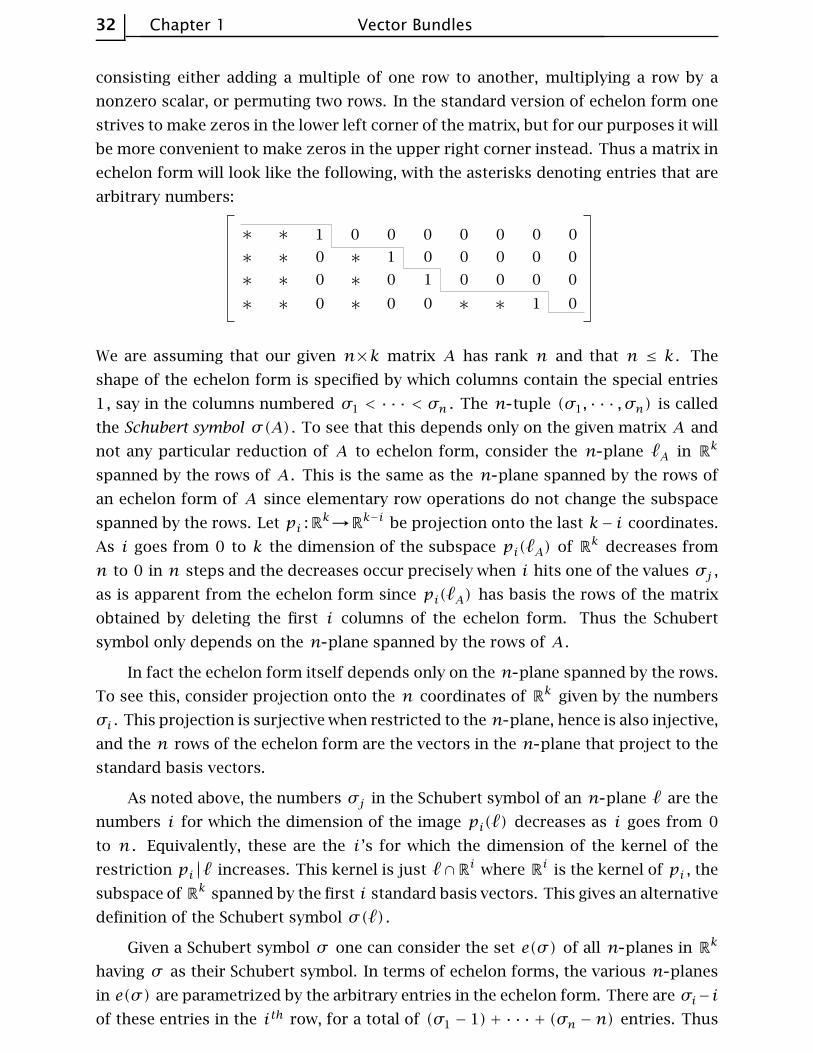
32 Chapter 1 Vector Bundles
consisting either adding a multiple of one row to another, multiplying a row by a
nonzero scalar, or permuting two rows. In the standard version of echelon form one
strives to make zeros in the lower left corner of the matrix, but for our purposes it will
be more convenient to make zeros in the upper right corner instead. Thus a matrix in
echelon form will look like the following, with the asterisks denoting entries that are
arbitrary numbers:
We are assuming that our given n×k matrix A has rank n and that n ≤ k . The
shape of the echelon form is specified by which columns contain the special entries
1, say in the columns numbered σ1 < · · · < σn . The n tuple (σ1, · · · , σn) is called
the Schubert symbol σ(A) . To see that this depends only on the given matrix A and
not any particular reduction of A to echelon form, consider the n plane ℓA in Rk
spanned by the rows of A . This is the same as the n plane spanned by the rows of
an echelon form of A since elementary row operations do not change the subspace
spanned by the rows. Let pi :Rk→R
k−i be projection onto the last k− i coordinates.
As i goes from 0 to k the dimension of the subspace pi(ℓA) of Rk decreases from
n to 0 in n steps and the decreases occur precisely when i hits one of the values σj ,
as is apparent from the echelon form since pi(ℓA) has basis the rows of the matrix
obtained by deleting the first i columns of the echelon form. Thus the Schubert
symbol only depends on the n plane spanned by the rows of A .
In fact the echelon form itself depends only on the n plane spanned by the rows.
To see this, consider projection onto the n coordinates of Rk given by the numbers
σi . This projection is surjective when restricted to the n plane, hence is also injective,
and the n rows of the echelon form are the vectors in the n plane that project to the
standard basis vectors.
As noted above, the numbers σj in the Schubert symbol of an n plane ℓ are the
numbers i for which the dimension of the image pi(ℓ) decreases as i goes from 0
to n . Equivalently, these are the i ’s for which the dimension of the kernel of the
restriction pi ||ℓ increases. This kernel is just ℓ∩Ri where Ri is the kernel of pi , the
subspace of Rk spanned by the first i standard basis vectors. This gives an alternative
definition of the Schubert symbol σ(ℓ) .
Given a Schubert symbol σ one can consider the set e(σ) of all n planes in Rk
having σ as their Schubert symbol. In terms of echelon forms, the various n planes
in e(σ) are parametrized by the arbitrary entries in the echelon form. There are σi−i
of these entries in the ith row, for a total of (σ1 − 1)+ · · · + (σn −n) entries. Thus
Classifying Vector Bundles Section 1.2 33
e(σ) is homeomorphic to a euclidean space of this dimension, or equivalently an open
cell.
Proposition 1.17. The cells e(σ) are the cells of a CW structure on Gn(Rk) .
For example G2(R4) has six cells corresponding to the Schubert symbols (1,2) ,
(1,3) , (1,4) , (2,3) , (2,4) , (3,4) , and these cells have dimensions 0, 1, 2, 2, 3, 4
respectively. In general the number of cells of Gn(Rk) is
(kn
), the number of ways of
choosing the n distinct numbers σi ≤ k .
Proof: Our main task will be to find a characteristic map for e(σ) . This is a map
from a closed ball of the same dimension as e(σ) into Gn(Rk) whose restriction
to the interior of the ball is a homeomorphism onto e(σ) . From the echelon forms
described above it is not clear how to do this, so we will use a slightly different sort
of echelon form. We allow the special 1’s to be arbitrary nonzero numbers and we
allow the entries below these 1’s to be nonzero. Then we impose the condition that
the rows be orthonormal and that the last nonzero entry in each row be positive. Let
us call this an orthonormal echelon form. Once again there is a unique orthonormal
echelon form for each n plane ℓ since if we let ℓi denote the subspace of ℓ spanned
by the first i rows of the standard echelon form, or in other words ℓi = ℓ ∩ Rσi ,
then there is a unique unit vector in ℓi orthogonal to ℓi−1 and having positive σith
coordinate.
The ith row of the orthonormal echelon form then belongs to the hemisphere Hiin the unit sphere Sσi−1 ⊂ Rσi ⊂ Rk consisting of unit vectors with non-negative σi
th
coordinate. In the Stiefel manifold Vn(Rk) let E(σ) be the subspace of orthonormal
frames (v1, · · · , vn) ∈ (Sk−1)n such that vi ∈ Hi for each i . We claim that E(σ) is
homeomorphic to a closed ball. To prove this the main step is to show that the pro-
jection π :E(σ)→H1 , π(v1, · · · , vn) = v1 , is a trivial fiber bundle. This is equivalent
to finding a projection p :E(σ)→π−1(v0) which is a homeomorphism on fibers of
π , where v0 = (0, · · · ,0,1) ∈ Rσ1 ⊂ Rk , since the map π×p :E(σ)→H1×π
−1(v0) is
then a continuous bijection of compact Hausdorff spaces, hence a homeomorphism.
The map p :π−1(v)→π−1(v0) is obtained by applying the rotation ρv of Rk that
takes v to v0 and fixes the (k − 2) dimensional subspace orthogonal to v and v0 .
This rotation takes Hi to itself for i > 1 since it affects only the first σ1 coordinates
of vectors in Rk . Hence p takes π−1(v) onto π−1(v0) .
The fiber π−1(v0) can be identified with E(σ ′) for σ ′ = (σ2 − 1, · · · , σn − 1) .
By induction on n this is homeomorphic to a closed ball of dimension (σ2 − 2) +
· · · + (σn −n) , so E(σ) is a closed ball of dimension (σ1 − 1)+ · · · + (σn −n) . The
boundary of this ball consists of points in E(σ) having vi in ∂Hi for at least one i .
This too follows by induction since the rotation ρv takes ∂Hi to itself for i > 1.
The natural map E(σ)→Gn sending an orthonormal n tuple to the n plane it
spans takes the interior of the ball E(σ) to e(σ) bijectively. Since Gn has the quotient
34 Chapter 1 Vector Bundles
topology from Vn , the map intE(σ)→e(σ) is a homeomorphism. The boundary of
E(σ) maps to cells e(σ ′) of Gn where σ ′ is obtained from σ by decreasing some
σi ’s, so these cells e(σ ′) have lower dimension than e(σ) .
To see that the maps E(σ)→Gn(Rk) for the cells e(σ) are the characteristic
maps for a CW structure on Gn(Rk) we can argue as follows. Let Xi be the union of
the cells e(σ) in Gn(Rk) having dimension at most i . Suppose by induction on i that
Xi is a CW complex with these cells. Attaching the (i+1) cells e(σ) of Xi+1 to Xi via
the maps ∂E(σ)→Xi produces a CW complex Y and a natural continuous bijection
Y→Xi+1 . Since Y is a finite CW complex it is compact, and Xi+1 is Hausdorff as a
subspace of Gn(Rk) , so the map Y→Xi+1 is a homeomorphism and Xi+1 is a CW
complex, finishing the induction. Thus we have a CW structure on Gn(Rk) . ⊔⊓
Since the inclusions Gn(Rk) ⊂ Gn(R
k+1) for varying k are inclusions of subcom-
plexes and Gn(R∞) has the weak topology with respect to these subspaces, it follows
that we have also a CW structure on Gn(R∞) .
Similar constructions work to give CW structures on complex Grassmann mani-
folds, but here e(σ) will be a cell of dimension (2σ1−2)+(2σ2−4)+· · ·+(2σn−2n) .
The hemisphere Hi is defined to be the subspace of the unit sphere S2σi−1 in Cσi con-
sisting of vectors whose σith coordinate is real and nonnegative, so Hi is a ball of
dimension 2σi − 2. The transformation ρv ∈ SU(k) is uniquely determined by spec-
ifying that it takes v to v0 and fixes the orthogonal (k − 2) dimensional complex
subspace, since an element of U(2) of determinant 1 is determined by where it sends
one unit vector.
The cell of Gn(Rk) of largest dimension is e(σ) for the Schubert symbol σ =
(k − n + 1, k − n + 2, · · · , k) . This cell has dimension n(k − n) , so this is the di-
mension of Gn(Rk) . Near points in this top-dimensional cell Gn(R
k) is a manifold.
But Gn(Rk) is homogeneous in the sense that given any two points in Gn(R
k) there
is a homeomorphism Gn(Rk)→Gn(Rk) taking one point to the other, namely, the
homeomorphism induced by an invertible linear map Rk→Rk taking one n plane to
the other. From this homogeneity it follows that Gn(Rk) is a manifold near all points.
Since it is compact, it is a closed manifold.
There is a natural inclusion i :Gn Gn+1 defined by i(ℓ) = R×j(ℓ) where
j :R∞→R∞ is the embedding j(x1, x2, · · ·) = (0, x1, x2, · · ·) . If σ(ℓ) = (σ1, · · · , σn)
then σ(i(ℓ)) = (1, σ1 + 1, · · · , σn + 1) , so i takes cells of Gn to cells of Gn+1 of the
same dimension, making i(Gn) a subcomplex of Gn+1 . Identifying Gn with the sub-
complex i(Gn) , we obtain an increasing sequence of CW complexes G1 ⊂ G2 ⊂ · · ·
whose union G∞ =⋃nGn is therefore also a CW complex. Similar remarks apply as
well in the complex case.
Appendix: Paracompactness 35
Appendix: Paracompactness
A Hausdorff space X is paracompact if for each open cover {Uα} of X there is
a partition of unity {ϕβ} subordinate to the cover. This means that the ϕβ ’s are
maps X→I such that each ϕβ has support (the closure of the set where ϕβ ≠ 0)
contained in some Uα , each x ∈ X has a neighborhood in which only finitely many
ϕβ ’s are nonzero, and∑βϕβ = 1. An equivalent definition which is often given is
that X is Hausdorff and every open cover of X has a locally finite open refinement.
The first definition clearly implies the second by taking the cover {ϕ−1β (0,1]} . For the
converse, see [Dugundji] or [Lundell-Weingram]. It is the former definition which is
most useful in algebraic topology, and the fact that the two definitions are equivalent
is rarely if ever needed. So we shall use the first definition.
A paracompact space X is normal, for let A1 and A2 be disjoint closed sets in X ,
and let {ϕβ} be a partition of unity subordinate to the cover {X−A1, X−A2} . Let ϕibe the sum of the ϕβ ’s which are nonzero at some point of Ai . Then ϕi(Ai) = 1, and
ϕ1 +ϕ2 ≤ 1 since no ϕβ can be a summand of both ϕ1 and ϕ2 . Hence ϕ−11 (
1/2,1]
and ϕ−12 (
1/2,1] are disjoint open sets containing A1 and A2 , respectively.
Most of the spaces one meets in algebraic topology are paracompact, including:
(1) compact Hausdorff spaces
(2) unions of increasing sequences X1 ⊂ X2 ⊂ · · · of compact Hausdorff spaces Xi ,
with the weak or direct limit topology (a set is open iff it intersects each Xi in an
open set)
(3) CW complexes
(4) metric spaces
Note that (2) includes (3) for CW complexes with countably many cells, since such
a CW complex can be expressed as an increasing union of finite subcomplexes. Using
(1) and (2), it can be shown that many manifolds are paracompact, for example Rn .
The next three propositions verify that the spaces in (1), (2), and (3) are paracom-
pact.
Proposition 1.18. A compact Hausdorff space X is paracompact.
Proof: Let {Uα} be an open cover of X . Since X is normal, each x ∈ X has an open
neighborhood Vx with closure contained in some Uα . By Urysohn’s lemma there is a
map ϕx :X→I with ϕx(x) = 1 and ϕx(X −Vx) = 0. The open cover {ϕ−1x (0,1]} of
X contains a finite subcover, and we relabel the corresponding ϕx ’s as ϕβ ’s. Then∑βϕβ(x) > 0 for all x , and we obtain the desired partition of unity subordinate to
{Uα} by normalizing each ϕβ by dividing it by∑βϕβ . ⊔⊓
Proposition 1.19. If X is the direct limit of an increasing sequence X1 ⊂ X2 ⊂ · · ·
of compact Hausdorff spaces Xi , then X is paracompact.

36 Chapter 1 Vector Bundles
Proof: A preliminary observation is that X is normal. To show this, it suffices to find
a map f :X→I with f(A) = 0 and f(B) = 1 for any two disjoint closed sets A and B .
Such an f can be constructed inductively over the Xi ’s, using normality of the Xi ’s.
For the induction step one has f defined on the closed set Xi∪(A∩Xi+1)∪(B∩Xi+1)
and one extends over Xi+1 by Tietze’s theorem.
To prove that X is paracompact, let an open cover {Uα} be given. Since Xi is
compact Hausdorff, there is a finite partition of unity {ϕij} on Xi subordinate to
{Uα ∩Xi} . Using normality of X , extend each ϕij to a map ϕij :X→I with support
in the same Uα . Let σi =∑jϕij . This sum is 1 on Xi , so if we normalize each ϕij
by dividing it by max{1/2, σi}, we get new maps ϕij with σi = 1 in a neighborhood
Vi of Xi . Let ψij =max{0,ϕij −∑k<iσk} . Since 0 ≤ ψij ≤ϕij , the collection {ψij}
is subordinate to {Uα} . In Vi all ψkj ’s with k > i are zero, so each point of X has a
neighborhood in which only finitely many ψij ’s are nonzero. For each x ∈ X there
is a ψij with ψij(x) > 0, since if ϕij(x) > 0 and i is minimal with respect to this
condition, then ψij(x) = ϕij(x) . Thus when we normalize the collection {ψij} by
dividing by∑i,jψij we obtain a partition of unity on X subordinate to {Uα} . ⊔⊓
Proposition 1.20. Every CW complex is paracompact.
Proof: Given an open cover {Uα} of a CW complex X , suppose inductively that we
have a partition of unity {ϕβ} on Xn subordinate to the cover {Uα ∩ Xn} . For a
cell en+1γ with characteristic map Φγ :Dn+1→X , {ϕβΦγ} is a partition of unity on
Sn = ∂Dn+1 . Since Sn is compact, only finitely many of these compositions ϕβΦγ can
be nonzero, for fixed γ . We extend these functions ϕβΦγ over Dn+1 by the formula
ρε(r)ϕβΦγ(x) using ‘spherical coordinates’ (r ,x) ∈ I×Sn on Dn+1 , where ρε : I→Iis 0 on [0,1−ε] and 1 on [1−ε/2,1]. If ε = εγ is chosen small enough, these extended
functions ρεϕβΦγ will be subordinate to the cover {Φ−1γ (Uα)} . Let {ψγj} be a finite
partition of unity on Dn+1 subordinate to {Φ−1γ (Uα)} . Then {ρεϕβΦγ , (1−ρε)ψγj} is
a partition of unity on Dn+1 subordinate to {Φ−1γ (Uα)} . This partition of unity extends
the partition of unity {ϕβΦγ} on Sn and induces an extension of {ϕβ} to a partition
of unity defined on Xn∪en+1γ and subordinate to {Uα} . Doing this for all (n+1) cells
en+1γ gives a partition of unity on Xn+1 . The local finiteness condition continues to
hold since near a point in Xn only the extensions of the ϕβ ’s in the original partition
of unity on Xn are nonzero, while in a cell en+1γ the only other functions that can be
nonzero are the ones coming from ψγj ’s. After we make such extensions for all n ,
we obtain a partition of unity defined on all of X and subordinate to {Uα} . ⊔⊓
Here is a technical fact about paracompact spaces that is occasionally useful:
Appendix: Paracompactness 37
Lemma 1.21. Given an open cover {Uα} of the paracompact space X , there is a
countable open cover {Vk} such that each Vk is a disjoint union of open sets each
contained in some Uα , and there is a partition of unity {ϕk} with ϕk supported in
Vk .
Proof: Let {ϕβ} be a partition of unity subordinate to {Uα} . For each finite set S of
functions ϕβ let VS be the subset of X where all the ϕβ ’s in S are strictly greater
than all the ϕβ ’s not in S . Since only finitely many ϕβ ’s are nonzero near any x ∈ X ,
VS is defined by finitely many inequalities among ϕβ ’s near x , so VS is open. Also,
VS is contained in some Uα , namely, any Uα containing the support of any ϕβ ∈ S ,
since ϕβ ∈ S implies ϕβ > 0 on VS . Let Vk be the union of all the open sets VS such
that S has k elements. This is clearly a disjoint union. The collection {Vk} is a cover
of X since if x ∈ X then x ∈ VS where S = {ϕβ | ϕβ(x) > 0 } .
For the second statement, let {ϕγ} be a partition of unity subordinate to the
cover {Vk} , and let ϕk be the sum of those ϕγ ’s supported in Vk but not in Vj for
j < k . ⊔⊓
Exercises
1. Show that the projection Vn(Rk)→Gn(Rk) is a fiber bundle with fiber O(n) by
showing that it is the orthonormal n frame bundle associated to the vector bundle
En(Rk)→Gn(Rk) .
The idea of K–theory is to make the direct sum operation on real or complex vector
bundles over a fixed base space X into the addition operation in a group. There are
two slightly different ways of doing this, producing, in the case of complex vector
bundles, groups K(X) and K(X) with K(X) ≈ K(X)⊕Z , and for real vector bundles,
groups KO(X) and KO(X) with KO(X) ≈ KO(X)⊕Z . Complex K–theory turns out
to be somewhat simpler than real K–theory, so we concentrate on this case in the
present chapter.
Computing K(X) even for simple spaces X requires some work. The case X = Sn
is the Bott Periodicity Theorem, which gives isomorphisms K(Sn) ≈ K(Sn+2) for all
n , and more generally K(X) ≈ K(S2X) where S2X is the double suspension of X .
This is a deep theorem, so it is not surprising that it has applications of real substance.
We give some of these in §2.3, notably:
(1) The nonexistence of division algebras over R in dimensions other than 1, 2, 4,
and 8, the dimensions of the real and complex numbers, quaternions, and Cayley
octonions.
(2) The nonparallelizability of spheres other than S1 , S3 , and S7 .
The proof of the Bott Periodicity Theorem divides into two parts. The first is the hard
technical work, proving an isomorphism K(X×S2) ≈ K(X)⊗K(S2) . This takes about
ten pages, forming the bulk of §2.1. The other half is easier, being more formal in
nature, and this is contained in §2.2 where the cohomological aspects of K(X) are
the main focus.
The Functor K(X) Section 2.1 39
2.1. The Functor K(X)
Since we shall be dealing exclusively with complex vector bundles in this chapter,
let us take ‘vector bundle’ to mean ‘complex vector bundle’ unless otherwise specified.
Base spaces will always be assumed to be compact Hausdorff, so that the results of
the preceding chapter which have this hypothesis will be available to us.
For the purposes of K–theory it is convenient to take a slightly broader defini-
tion of ‘vector bundle’ which allows the fibers of a vector bundle p :E→X to be vec-
tor spaces of different dimensions. We still assume local trivializations of the form
h :p−1(U)→U×Cn , so the dimensions of fibers must be locally constant over X , but
if X is disconnected the dimensions of fibers need not be globally constant.
Consider vector bundles over a fixed base space X . The trivial n dimensional
vector bundle we write as εn→X . Define two vector bundles E1 and E2 over X to be
stably isomorphic, written E1 ≈s E2 , if E1⊕εn ≈ E2⊕ε
n for some n . In a similar vein
we set E1 ∼ E2 if E1⊕εm ≈ E2⊕ε
n for some m and n . It is easy to see that both ≈s
and ∼ are equivalence relations. On equivalence classes of either sort the operation
of direct sum is well-defined, commutative, and associative. A zero element is the
class of ε0 .
Proposition 2.1. If X is compact Hausdorff, then the set of ∼ equivalence classes of
vector bundles over X forms an abelian group with respect to ⊕ .
This group is called K(X) .
Proof: Only the existence of inverses needs to be shown, which we do by showing
that for each vector bundle π :E→X there is a bundle E′→X such that E⊕E′ ≈ εm
for some m . If all the fibers of E have the same dimension, this is Proposition 1.4.
In the general case let Xi = {x ∈ X || dimπ−1(x) = i } . These Xi ’s are disjoint open
sets in X , hence are finite in number by compactness. By adding to E a bundle which
over each Xi is a trivial bundle of suitable dimension we can produce a bundle whose
fibers all have the same dimension. ⊔⊓
For the direct sum operation on ≈s equivalence classes, only the zero element, the
class of ε0 , can have an inverse since E⊕E′ ≈s ε0 implies E⊕E′⊕εn ≈ εn for some
n , which can only happen if E and E′ are 0 dimensional. However, even though
inverses do not exist, we do have the cancellation property that E1⊕E2 ≈s E1⊕E3
implies E2 ≈s E3 over a compact base space X , since we can add to both sides of
E1⊕E2 ≈s E1⊕E3 a bundle E′1 such that E1⊕E′1 ≈ ε
n for some n .
Just as the positive rational numbers are constructed from the positive integers
by forming quotients a/b with the equivalence relation a/b = c/d iff ad = bc , so we
can form for compact X an abelian group K(X) consisting of formal differences E−E′
of vector bundles E and E′ over X , with the equivalence relation E1 − E′1 = E2 − E
′2
iff E1⊕E′2 ≈s E2⊕E
′1 . Verifying transitivity of this relation involves the cancellation
40 Chapter 2 Complex K–Theory
property, which is why compactness of X is needed. With the obvious addition rule
(E1−E′1)+(E2−E
′2) = (E1⊕E2)−(E
′1⊕E
′2) , K(X) is then a group. The zero element is
the equivalence class of E−E for any E , and the inverse of E−E′ is E′−E . Note that
every element of K(X) can be represented as a difference E−εn since if we start with
E − E′ we can add to both E and E′ a bundle E′′ such that E′⊕E′′ ≈ εn for some n .
There is a natural homomorphism K(X)→K(X) sending E − εn to the ∼ class
of E . This is well-defined since if E − εn = E′ − εm in K(X) , then E⊕εm ≈s E′⊕εn ,
hence E ∼ E′ . The map K(X)→K(X) is obviously surjective, and its kernel consists of
elements E−εn with E ∼ ε0 , hence E ≈s εm for some m , so the kernel consists of the
elements of the form εm − εn . This subgroup {εm − εn} of K(X) is isomorphic to Z .
In fact, restriction of vector bundles to a basepoint x0 ∈ X defines a homomorphism
K(X)→K(x0) ≈ Z which restricts to an isomorphism on the subgroup {εm − εn} .
Thus we have a splitting K(X) ≈ K(X)⊕Z , depending on the choice of x0 . The group
K(X) is sometimes called reduced , to distinguish it from K(X) .
Ring Structure
Besides the additive structure in K(X) there is also a natural multiplication com-
ing from tensor product of vector bundles. For elements of K(X) represented by
vector bundles E1 and E2 their product in K(X) will be represented by the bundle
E1⊗E2 , so for arbitrary elements of K(X) represented by differences of vector bun-
dles, their product in K(X) is defined by the formula
(E1 − E′1)(E2 − E
′2) = E1⊗E2 − E1⊗E
′2 − E
′1⊗E2 + E
′1⊗E
′2
It is routine to verify that this is well-defined and makes K(X) into a commutative ring
with identity ε1 , the trivial line bundle, using the basic properties of tensor product
of vector bundles described in §1.1. We can simplify notation by writing the element
εn ∈ K(X) just as n . This is consistent with familiar arithmetic rules. For example,
the product nE is the sum of n copies of E .
If we choose a basepoint x0 ∈ X , then the map K(X)→K(x0) obtained by re-
stricting vector bundles to their fibers over x0 is a ring homomorphism. Its kernel,
which can be identified with K(X) as we have seen, is an ideal, hence also a ring in its
own right, though not necessarily a ring with identity.
The rings K(X) and K(X) can be regarded as functors of X . A map f :X→Y in-
duces a map f∗ :K(Y)→K(X) , sending E−E′ to f∗(E)−f∗(E′) . This is a ring homo-
morphism since f∗(E1⊕E2) ≈ f∗(E1)⊕f
∗(E2) and f∗(E1⊗E2) ≈ f∗(E1)⊗f
∗(E2) .
The functor properties (fg)∗ = g∗f∗ and 11∗ = 11 as well as the fact that f ≃ g
implies f∗ = g∗ all follow from the corresponding properties for pullbacks of vector
bundles. Similarly, we have induced maps f∗ : K(Y )→K(X) with the same properties,
except that for f∗ to be a ring homomorphism we must be in the category of base-
The Functor K(X) Section 2.1 41
pointed spaces and basepoint-preserving maps since our definition of multiplication
for K required basepoints.
An external product µ :K(X)⊗K(Y)→K(X×Y) can be defined by µ(a⊗b) =
p∗1 (a)p∗2 (b) where p1 and p2 are the projections of X×Y onto X and Y . The tensor
product of rings is a ring, with multiplication defined by (a⊗b)(c ⊗d) = ac ⊗bd , and
µ is a ring homomorphism since µ((a⊗b)(c ⊗d)) = µ(ac ⊗bd) = p∗1 (ac)p∗2 (bd) =
p∗1 (a)p∗1 (c)p
∗2 (b)p
∗2 (d) = p
∗1 (a)p
∗2 (b)p
∗1 (c)p
∗2 (d) = µ(a⊗b)µ(c ⊗d) .
Taking Y to be S2 we have an external product
µ :K(X)⊗K(S2)→K(X×S2)
Most of the remainder of §2.1 will be devoted to showing that this map is an isomor-
phism. This is the essential core of the proof of Bott Periodicity.
The external product in ordinary cohomology is called ‘cross product’ and written
a×b , but to use this symbol for the K–theory external product might lead to confusion
with Cartesian product of vector bundles, which is quite different from tensor product.
Instead we will sometimes use the notation a∗ b as shorthand for µ(a⊗b) .
The Fundamental Product Theorem
The key result allowing the calculation of K(X) in nontrivial cases is a certain for-
mula that computes K(X×S2) in terms of K(X) . For example, when X is a point this
will yield a calculation of K(S2) . In the next section we will deduce other calculations,
in particular K(Sn) for all n .
Let H be the canonical line bundle over S2 = CP1 . We showed in Example 1.13
that (H⊗H)⊕1 ≈ H⊕H . In K(S2) this is the formula H2+1 = 2H , so H2 = 2H−1.
We can also write this as (H − 1)2 = 0, so we have a natural ring homomorphism
Z[H]/(H − 1)2→K(S2) whose domain is the quotient ring of the polynomial ring
Z[H] by the ideal generated by (H −1)2 . In particular, note that an additive basis for
Z[H]/(H − 1)2 is {1,H} .
We define a homomorphism µ as the composition
µ :K(X)⊗Z[H]/(H − 1)2 -→K(X)⊗K(S2) -→K(X×S2)
where the second map is the external product.
Theorem 2.2. The homomorphism µ :K(X)⊗Z[H]/(H − 1)2→K(X×S2) is an iso-
morphism of rings for all compact Hausdorff spaces X .
Taking X to be a point we obtain:
Corollary 2.3. The map Z[H]/(H − 1)2→K(S2) is an isomorphism of rings.
Thus if we regard K(S2) as the kernel of K(S2)→K(x0) , then it is generated as
an abelian group by H − 1. Since we have the relation (H − 1)2 = 0, this means that
42 Chapter 2 Complex K–Theory
the multiplication in K(S2) is completely trivial: The product of any two elements
is zero. Readers familiar with cup product in ordinary cohomology will recognize
that the situation is exactly the same as in H∗(S2;Z) and H∗(S2;Z) , with H − 1
behaving exactly like the generator of H2(S2;Z) . In the case of ordinary cohomology
the cup product of a generator of H2(S2;Z) with itself is automatically zero since
H4(S2;Z) = 0, whereas with K–theory a calculation is required.
The present section will be devoted entirely to the proof of the preceding theorem.
Nothing in the proof will be used elsewhere in the book except in the proof of Bott
periodicity for real K–theory in §2.4, so the reader who wishes to defer a careful
reading of the proof may skip ahead to §2.2 without any loss of continuity.
The main work in proving the theorem will be to prove the surjectivity of µ .
Injectivity will then be proved by a closer examination of the surjectivity argument.
Clutching Functions
From the classification of vector bundles over spheres in §1.2 we know that vec-
tor bundles over S2 correspond exactly to homotopy classes of maps S1→GLn(C) ,which we called clutching functions. To prove the theorem we will generalize this con-
struction, creating vector bundles over X×S2 by gluing together two vector bundles
over X×D2 by means of a generalized clutching function.
We begin by describing this more general clutching construction. Given a vector
bundle p :E→X , let f :E×S1→E×S1 be an automorphism of the product vector
bundle p×11 :E×S1→X×S1 . Thus for each x ∈ X and z ∈ S1 , f specifies an
isomorphism f(x, z) :p−1(x)→p−1(x) . From E and f we construct a vector bundle
over X×S2 by taking two copies of E×D2 and identifying the subspaces E×S1 via
f . We write this bundle as [E, f ] , and call f a clutching function for [E, f ] . If
ft :E×S1→E×S1 is a homotopy of clutching functions, then [E, f0] ≈ [E, f1] since
from the homotopy ft we can construct a vector bundle over X×S2×I restricting
to [E, f0] and [E, f1] over X×S2×{0} and X×S2×{1} . From the definitions it is
evident that [E1, f1]⊕[E2, f2] ≈ [E1⊕E2, f1 ⊕ f2] .
Here are some examples of bundles built using clutching functions:
1. [E,11] is the external product E ∗ 1 = µ(E⊗1) , or equivalently the pullback of E
via the projection X×S2→X .
2. Taking X to be a point, then we showed in Example 1.10 that [1, z] ≈ H where ‘1’
is the trivial line bundle over X , ‘z ’ means scalar multiplication by z ∈ S1 ⊂ C , and
H is the canonical line bundle over S2 = CP1 . More generally we have [1, zn] ≈ Hn ,
the n fold tensor product of H with itself. The formula [1, zn] ≈ Hn holds also for
negative n if we define H−1 = [1, z−1] , which is justified by the fact that H⊗H−1 ≈ 1.
3. [E, zn] ≈ E ∗Hn = µ(E⊗Hn) for n ∈ Z .
4. Generalizing this, [E, znf] ≈ [E, f ]⊗Hn where Hn denotes the pullback of Hn
via the projection X×S2→S2 .
The Functor K(X) Section 2.1 43
Every vector bundle E′→X×S2 is isomorphic to [E, f ] for some E and f . To
see this, let the unit circle S1 ⊂ C ∪ {∞} = S2 decompose S2 into the two disks D0
and D∞ , and let Eα for α = 0,∞ be the restriction of E′ over X×Dα , with E the
restriction of E′ over X×{1} . The projection X×Dα→X×{1} is homotopic to the
identity map of X×Dα , so the bundle Eα is isomorphic to the pullback of E by the
projection, and this pullback is E×Dα , so we have an isomorphism hα :Eα→E×Dα .
Then f = h0h−1∞ is a clutching function for E′ .
We may assume a clutching function f is normalized to be the identity over
X×{1} since we may normalize any isomorphism hα :Eα→E×Dα by composing it
over each X×{z} with the inverse of its restriction over X×{1} . For the given vector
bundle E′ any two choices of normalized hα are homotopic through normalized hα ’s
since they differ by a map gα from Dα to the automorphisms of E , with gα(1) = 11,
and such a gα is homotopic to the constant map 11 by composing it with a deformation
retraction of Dα to 1. Thus any two choices f0 and f1 of normalized clutching
functions are joined by a homotopy of normalized clutching functions ft .
The strategy of the proof will be to reduce from arbitrary clutching functions
to successively simpler clutching functions. The first step is to reduce to Laurent
polynomial clutching functions, which have the form ℓ(x, z) =∑|i|≤n ai(x)z
i where
ai :E→E restricts to a linear transformation ai(x) in each fiber p−1(x) . We call
such an ai an endomorphism of E since the linear transformations ai(x) need not
be invertible, though their linear combination∑i ai(x)z
i is since clutching functions
are automorphisms.
Proposition 2.4. Every vector bundle [E, f ] is isomorphic to [E, ℓ] for some Laurent
polynomial clutching function ℓ . Laurent polynomial clutching functions ℓ0 and
ℓ1 which are homotopic through clutching functions are homotopic by a Laurent
polynomial clutching function homotopy ℓt(x, z) =∑i ai(x, t)z
i .
Before beginning the proof we need a lemma. For a compact space X we wish
to approximate a continuous function f :X×S1→C by Laurent polynomial functions∑|n|≤N an(x)z
n =∑|n|≤N an(x)e
inθ , where z = eiθ and each an is a continuous
function X→C . Motivated by Fourier series, we set
an(x) =1
2π
∫ 2π
0f(x, eiθ)e−inθ dθ
For positive real r let u(x, r , θ) =∑n∈Z an(x)r
|n|einθ . For fixed r < 1, this se-
ries converges absolutely and uniformly as (x, θ) ranges over X×[0,2π] , by com-
parison with the geometric series∑n r
n , since compactness of X×S1 implies that
|f(x, eiθ)| is bounded and hence also |an(x)| . If we can show that u(x, r , θ) ap-
proaches f(x, eiθ) uniformly in x and θ as r goes to 1, then sums of finitely many
terms in the series for u(x, r , θ) with r near 1 will give the desired approximations
to f by Laurent polynomial functions.
44 Chapter 2 Complex K–Theory
Lemma 2.5. As r→1 , u(x, r , θ)→f(x, eiθ) uniformly in x and θ .
Proof: For r < 1 we have
u(x, r , θ) =∞∑
n=−∞
1
2π
∫ 2π
0r |n|ein(θ−t)f(x, eit)dt
=
∫ 2π
0
1
2π
∞∑n=−∞
r |n|ein(θ−t)f(x, eit)dt
where the order of summation and integration can be interchanged since the series
in the latter formula converges uniformly, by comparison with the geometric series∑n r
n . Define the Poisson kernel
P(r ,ϕ) =1
2π
∞∑n=−∞
r |n|einϕ for 0 ≤ r < 1 and ϕ ∈ R
Then u(x, r , θ) =� 2π
0P(r , θ − t)f (x, eit)dt . By summing the two geometric series
for positive and negative n in the formula for P(r ,ϕ) , one computes that
P(r ,ϕ) =1
2π·
1− r 2
1− 2r cosϕ + r 2
Three basic facts about P(r ,ϕ) which we shall need are:
(a) As a function of ϕ , P(r ,ϕ) is even, of period 2π , and monotone decreasing
on [0, π] , since the same is true of cosϕ which appears in the denominator of
P(r ,ϕ) with a minus sign. In particular we have P(r ,ϕ) ≥ P(r ,π) > 0 for all
r < 1.
(b)� 2π
0P(r ,ϕ)dϕ = 1 for each r < 1, as one sees by integrating the series for
P(r ,ϕ) term by term.
(c) For fixed ϕ ∈ (0, π) , P(r ,ϕ)→0 as r→1 since the numerator of P(r ,ϕ) ap-
proaches 0 and the denominator approaches 2− 2 cosϕ ≠ 0.
Now to show uniform convergence of u(x, r , θ) to f(x, eiθ) we first observe that,
using (b), we have
∣∣u(x, r , θ)− f(x, eiθ)∣∣ =
∣∣∣∫ 2π
0P(r , θ − t)f (x, eit)dt −
∫ 2π
0P(r , θ − t)f (x, eiθ)dt
∣∣∣
≤
∫ 2π
0P(r , θ − t)
∣∣f(x, eit)− f(x, eiθ)∣∣dt
Given ε > 0, there exists a δ > 0 such that |f(x, eit)− f(x, eiθ)| < ε for |t − θ| < δ
and all x , since f is uniformly continuous on the compact space X×S1 . Let Iδ denote
the integral�P(r , θ− t) |f(x, eit)− f(x, eiθ)|dt over the interval |t−θ| ≤ δ and let
I′δ denote this integral over the complement of the interval |t − θ| ≤ δ in an interval
of length 2π . Then we have
Iδ ≤
∫
|t−θ|≤δP(r , θ − t) ε dt ≤ ε
∫ 2π
0P(r , θ − t)dt = ε
The Functor K(X) Section 2.1 45
By (a) the maximum value of P(r , θ − t) on |t − θ| ≥ δ is P(r , δ) . So
I′δ ≤ P(r , δ)
∫ 2π
0|f(x, eit)− f(x, eiθ)|dt
The integral here has a uniform bound for all x and θ since f is bounded. Thus by (c)
we can make I′δ ≤ ε by taking r close enough to 1. Therefore |u(x, r , θ)−f(x,θ)| ≤
Iδ + I′δ ≤ 2ε . ⊔⊓
Proof of Proposition 2.4: Choosing a Hermitian inner product on E , the endomor-
phisms of E×S1 form a vector space End(E×S1) with a norm ‖α‖ = sup|v|=1 |α(v)| .
The triangle inequality holds for this norm, so balls in End(E×S1) are convex. The
subspace Aut(E×S1) of automorphisms is open in the topology defined by this norm
since it is the preimage of (0,∞) under the continuous map End(E×S1)→[0,∞) ,α֏ inf(x,z)∈X×S1|det(α(x, z))| . Thus to prove the first statement of the proposi-
tion it will suffice to show that Laurent polynomials are dense in End(E×S1) , since
a sufficiently close Laurent polynomial approximation ℓ to f will then be homotopic
to f via the linear homotopy tℓ+ (1− t)f through clutching functions. The second
statement follows similarly by approximating a homotopy from ℓ0 to ℓ1 , viewed as an
automorphism of E×S1×I , by a Laurent polynomial homotopy ℓ′t , then combining
this with linear homotopies from ℓ0 to ℓ′0 and ℓ1 to ℓ′1 to obtain a homotopy ℓt from
ℓ0 to ℓ1 .
To show that every f ∈ End(E×S1) can be approximated by Laurent polynomial
endomorphisms, first choose open sets Ui covering X together with isomorphisms
hi :p−1(Ui)→Ui×Cni . We may assume hi takes the chosen inner product in p−1(Ui)
to the standard inner product in Cni , by applying the Gram-Schmidt process to h−1
i
of the standard basis vectors. Let {ϕi} be a partition of unity subordinate to {Ui}
and let Xi be the support of ϕi , a compact set in Ui . Via hi , the linear maps f(x, z)
for x ∈ Xi can be viewed as matrices. The entries of these matrices define functions
Xi×S1→C . By the lemma we can find Laurent polynomial matrices ℓi(x, z) whose
entries uniformly approximate those of f(x, z) for x ∈ Xi . It follows easily that ℓiapproximates f in the ‖ · ‖ norm. From the Laurent polynomial approximations ℓiover Xi we form the convex linear combination ℓ =
∑iϕiℓi , a Laurent polynomial
approximating f over all of X×S1 . ⊔⊓
A Laurent polynomial clutching function can be written ℓ = z−mq for a polyno-
mial clutching function q , and then we have [E, ℓ] ≈ [E, q]⊗H−m . The next step is
to reduce polynomial clutching functions to linear clutching functions.
Proposition 2.6. If q is a polynomial clutching function of degree at most n , then
[E, q]⊕[nE,11] ≈ [(n+ 1)E, Lnq] for a linear clutching function Lnq .
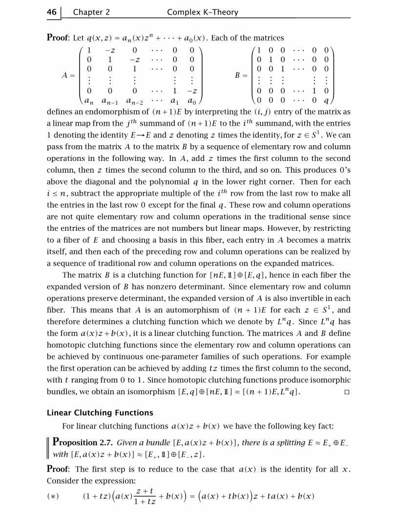
46 Chapter 2 Complex K–Theory
Proof: Let q(x, z) = an(x)zn + · · · + a0(x) . Each of the matrices
A =
1 −z 0 · · · 0 0
0 1 −z · · · 0 0
0 0 1 · · · 0 0...
......
......
0 0 0 · · · 1 −zan an−1 an−2 · · · a1 a0
B =
1 0 0 · · · 0 0
0 1 0 · · · 0 0
0 0 1 · · · 0 0...
......
......
0 0 0 · · · 1 0
0 0 0 · · · 0 q
defines an endomorphism of (n+1)E by interpreting the (i, j) entry of the matrix as
a linear map from the j th summand of (n+1)E to the ith summand, with the entries
1 denoting the identity E→E and z denoting z times the identity, for z ∈ S1 . We can
pass from the matrix A to the matrix B by a sequence of elementary row and column
operations in the following way. In A , add z times the first column to the second
column, then z times the second column to the third, and so on. This produces 0’s
above the diagonal and the polynomial q in the lower right corner. Then for each
i ≤ n , subtract the appropriate multiple of the ith row from the last row to make all
the entries in the last row 0 except for the final q . These row and column operations
are not quite elementary row and column operations in the traditional sense since
the entries of the matrices are not numbers but linear maps. However, by restricting
to a fiber of E and choosing a basis in this fiber, each entry in A becomes a matrix
itself, and then each of the preceding row and column operations can be realized by
a sequence of traditional row and column operations on the expanded matrices.
The matrix B is a clutching function for [nE,11]⊕[E, q] , hence in each fiber the
expanded version of B has nonzero determinant. Since elementary row and column
operations preserve determinant, the expanded version of A is also invertible in each
fiber. This means that A is an automorphism of (n + 1)E for each z ∈ S1 , and
therefore determines a clutching function which we denote by Lnq . Since Lnq has
the form a(x)z+b(x) , it is a linear clutching function. The matrices A and B define
homotopic clutching functions since the elementary row and column operations can
be achieved by continuous one-parameter families of such operations. For example
the first operation can be achieved by adding tz times the first column to the second,
with t ranging from 0 to 1. Since homotopic clutching functions produce isomorphic
bundles, we obtain an isomorphism [E, q]⊕[nE,11] ≈ [(n+ 1)E, Lnq] . ⊔⊓
Linear Clutching Functions
For linear clutching functions a(x)z + b(x) we have the following key fact:
Proposition 2.7. Given a bundle [E,a(x)z+ b(x)] , there is a splitting E ≈ E+⊕E−with [E,a(x)z + b(x)] ≈ [E+,11]⊕[E−, z] .
Proof: The first step is to reduce to the case that a(x) is the identity for all x .
Consider the expression:
(∗) (1+ tz)(a(x)
z + t
1+ tz+ b(x)
)=(a(x)+ tb(x)
)z + ta(x)+ b(x)
The Functor K(X) Section 2.1 47
When t = 0 this equals a(x)z + b(x) . For 0 ≤ t < 1, (∗) defines an invertible
linear transformation since the left-hand side is obtained from a(x)z+ b(x) by first
applying the substitution z֏ (z + t)/(1 + tz) which takes S1 to itself (because if
|z| = 1 then |(z+t)/(1+tz)| = |z(z+t)/(1+tz)| = |(1+tz)/(1+tz)| = |w/w| = 1),
and then multiplying by the nonzero scalar 1+tz . Therefore (∗) defines a homotopy
of clutching functions as t goes from 0 to t0 < 1. In the right-hand side of (∗) the
term a(x) + tb(x) is invertible for t = 1 since it is the restriction of a(x)z + b(x)
to z = 1. Therefore a(x) + tb(x) is invertible for t = t0 near 1, as the continuous
function t֏ infx∈X∣∣det
(a(x)+ tb(x)
)∣∣ is nonzero for t = 1, hence also for t near
1. Now we use the simple fact that [E, fg] ≈ [E, f ] for any isomorphism g :E→E .
This allows us to replace the clutching function on the right-hand side of (∗) by the
clutching function z +(t0a(x) + b(x)
)(a(x) + t0b(x)
)−1, reducing to the case of
clutching functions of the form z + b(x) .
Since z + b(x) is invertible for all x , b(x) has no eigenvalues on the unit circle
S1 .
Lemma 2.8. Let b :E→E be an endomorphism having no eigenvalues on the unit
circle S1 . Then there are unique subbundles E+ and E− of E such that :
(a) E = E+⊕E− .
(b) b(E±) ⊂ E± .
(c) The eigenvalues of b ||E+ all lie outside S1 and the eigenvalues of b ||E− all lie
inside S1 .
Proof: Consider first the algebraic situation of a linear transformation T :V→V with
characteristic polynomial q(t) . Assuming q(t) has no roots on S1 , we may factor q(t)
in C[t] as q+(t)q−(t) where q+(t) has all its roots outside S1 and q−(t) has all its
roots inside S1 . Let V± be the kernel of q±(T) :V→V . Since q+ and q− are relatively
prime in C[t] , there are polynomials r and s with rq++sq− = 1. From q+(T)q−(T) =
q(T) = 0, we have Imq−(T) ⊂ Kerq+(T) , and the opposite inclusion follows from
r(T)q+(T)+ q−(T)s(T) = 11. Thus Kerq+(T) = Imq−(T) , and similarly Kerq−(T) =
Imq+(T) . From q+(T)r(T) + q−(T)s(T) = 11 we see that Imq+(T) + Imq−(T) = V ,
and from r(T)q+(T) + s(T)q−(T) = 11 we deduce that Kerq+(T) ∩ Kerq−(T) = 0.
Hence V = V+⊕V− . We have T(V±) ⊂ V± since q±(T)(v) = 0 implies q±(T)(T(v)) =
T(q±(T)(v)) = 0. All eigenvalues of T ||V± are roots of q± since q±(T) = 0 on V± .
Thus conditions (a)–(c) hold for V+ and V− .
To see the uniqueness of V+ and V− satisfying (a)–(c), let q′± be the characteristic
polynomial of T ||V± , so q = q′+q′− . All the linear factors of q′± must be factors of
q± by condition (c), so the factorizations q = q′+q′− and q = q+q− must coincide up
to scalar factors. Since q′±(T) is identically zero on V± , so must be q±(T) , hence
V± ⊂ Kerq±(T) . Since V = V+⊕V− and V = Kerq+(T)⊕ Kerq−(T) , we must have
V± = Kerq±(T) . This establishes the uniqueness of V± .
48 Chapter 2 Complex K–Theory
As T varies continuously through linear transformations without eigenvalues on
S1 , its characteristic polynomial q(t) varies continuously through polynomials with-
out roots in S1 . In this situation we assert that the factors q± of q vary continuously
with q , assuming that q , q+ , and q− are normalized to be monic polynomials. To
see this we shall use the fact that for any circle C in C disjoint from the roots of q ,
the number of roots of q inside C , counted with multiplicity, equals the degree of
the map γ :C→S1 , γ(z) = q(z)/|q(z)| . To prove this fact consider first the case of
a small circle C about a root z = a of multiplicity m , so q(t) = p(t)(t − a)m with
p(a) ≠ 0. The homotopy
γs(z) =p(sa+ (1− s)z
)(z − a)m
|p(sa+ (1− s)z
)(z − a)m|
gives a reduction to the case (t − a)m , where it is clear that the degree is m . As
the circle C is gradually enlarged, the map γ changes only by homotopy, leaving its
degree unchanged, except when C is enlarged to enclose another root of q . In this
case the new loop C is homotopic to the composition of the old loop C with a small
loop about the new root, so the degree of γ for the new C is the sum of the old degree
plus the degree for the small loop. The result then follows by induction.
For a small circle C about a root z = a of q of multiplicity m , small perturbations
of q to nearby polynomials q′ produce small perturbations of the map γ to nearby
maps γ′ which are therefore homotopic to γ , having the same degree, hence q′ also
has m roots a1, · · · , am inside C . Thus the factor (z − a)m of q becomes a factor
(z−a1) · · · (z−am) of the nearby q′ . Since the ai ’s are near a , the factor (z−a)m of
q is close to the factor (z−a1) · · · (z−am) of q′ since multiplication of polynomials
is a continuous operation. Taking the products of these factors for the roots inside
or outside the unit circle, we conclude that q′± is close to q± , so the factorization
q = q+q− varies continuously with q , as claimed.
Next we observe that as T varies continuously through transformations without
eigenvalues in S1 , the splitting V = V+⊕V− also varies continuously. To see this,
recall that V+ = Imq−(T) and V− = Imq+(T) . Choose a basis v1, · · · , vn for V such
that q−(T)(v1), · · · , q−(T)(vk) is a basis for V+ and q+(T)(vk+1), · · · , q+(T)(vn) is
a basis for V− . For nearby T these vectors vary continuously, hence remain indepen-
dent. Thus the splitting V = Imq−(T)⊕ Imq+(T) continues to hold for nearby T ,
and so the splitting V = V+⊕V− varies continuously with T .
It follows that the union E± of the subspaces V± in all the fibers V of E is a
subbundle, and so the proof of the lemma is complete. ⊔⊓
To finish the proof of Proposition 2.7, note that the lemma gives a splitting [E, z+
b(x)] ≈ [E+, z + b+(x)]⊕[E−, z + b−(x)] where b+ and b− are the restrictions of
b . Since b+(x) has all its eigenvalues outside S1 , the formula tz + b+(x) for 0 ≤
t ≤ 1 defines a homotopy of clutching functions from z + b+(x) to b+(x) . Hence
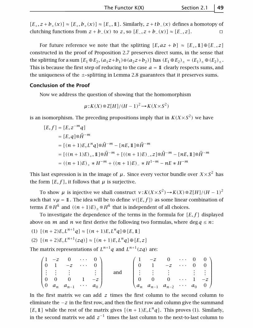
The Functor K(X) Section 2.1 49
[E+, z+b+(x)] ≈ [E+, b+(x)] ≈ [E+,11] . Similarly, z+ tb−(x) defines a homotopy of
clutching functions from z + b−(x) to z , so [E−, z + b−(x)] ≈ [E−, z] . ⊔⊓
For future reference we note that the splitting [E,az + b] ≈ [E+,11]⊕[E−, z]
constructed in the proof of Proposition 2.7 preserves direct sums, in the sense that
the splitting for a sum [E1⊕E2, (a1z+b1)⊕(a2z+b2)] has (E1⊕E2)± = (E1)±⊕(E2)± .
This is because the first step of reducing to the case a = 11 clearly respects sums, and
the uniqueness of the ± splitting in Lemma 2.8 guarantees that it preserves sums.
Conclusion of the Proof
Now we address the question of showing that the homomorphism
µ :K(X)⊗Z[H]/(H − 1)2→K(X×S2)
is an isomorphism. The preceding propositions imply that in K(X×S2) we have
[E, f ] = [E, z−mq]
= [E, q]⊗H−m
= [(n+ 1)E, Lnq]⊗H−m − [nE,11]⊗H−m
= [((n+ 1)E)+,11]⊗H−m + [((n+ 1)E)−, z]⊗H
−m − [nE,11]⊗H−m
= ((n+ 1)E)+ ∗H−m + ((n+ 1)E)− ∗H
1−m −nE ∗H−m
This last expression is in the image of µ . Since every vector bundle over X×S2 has
the form [E, f ] , it follows that µ is surjective.
To show µ is injective we shall construct ν :K(X×S2)→K(X)⊗Z[H]/(H − 1)2
such that νµ = 11. The idea will be to define ν([E, f ]) as some linear combination of
terms E⊗Hk and ((n+ 1)E)±⊗Hk that is independent of all choices.
To investigate the dependence of the terms in the formula for [E, f ] displayed
above on m and n we first derive the following two formulas, where degq ≤ n :
(1) [(n+ 2)E, Ln+1q] ≈ [(n+ 1)E, Lnq]⊕[E,11]
(2) [(n+ 2)E, Ln+1(zq)] ≈ [(n+ 1)E, Lnq]⊕[E, z]
The matrix representations of Ln+1q and Ln+1(zq) are:
1 −z 0 · · · 0
0 1 −z · · · 0...
......
...
0 0 0 1 −z0 an an−1 · · · a0
and
1 −z 0 · · · 0 0
0 1 −z · · · 0 0...
......
......
0 0 0 · · · 1 −zan an−1 an−2 · · · a0 0
In the first matrix we can add z times the first column to the second column to
eliminate the −z in the first row, and then the first row and column give the summand
[E,11] while the rest of the matrix gives [(n + 1)E, Lnq] . This proves (1). Similarly,
in the second matrix we add z−1 times the last column to the next-to-last column to
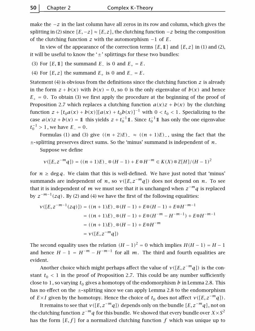
50 Chapter 2 Complex K–Theory
make the −z in the last column have all zeros in its row and column, which gives the
splitting in (2) since [E,−z] ≈ [E, z] , the clutching function −z being the composition
of the clutching function z with the automorphism −1 of E .
In view of the appearance of the correction terms [E,11] and [E, z] in (1) and (2),
it will be useful to know the ‘± ’ splittings for these two bundles:
(3) For [E,11] the summand E− is 0 and E+ = E .
(4) For [E, z] the summand E+ is 0 and E− = E .
Statement (4) is obvious from the definitions since the clutching function z is already
in the form z + b(x) with b(x) = 0, so 0 is the only eigenvalue of b(x) and hence
E+ = 0. To obtain (3) we first apply the procedure at the beginning of the proof of
Proposition 2.7 which replaces a clutching function a(x)z + b(x) by the clutching
function z + [t0a(x) + b(x)][a(x) + t0b(x)]−1 with 0 < t0 < 1. Specializing to the
case a(x)z + b(x) = 11 this yields z + t−10 11. Since t−1
0 11 has only the one eigenvalue
t−10 > 1, we have E− = 0.
Formulas (1) and (3) give ((n + 2)E)− ≈ ((n + 1)E)− , using the fact that the
± splitting preserves direct sums. So the ‘minus’ summand is independent of n .
Suppose we define
ν([E, z−mq]) = ((n+ 1)E)−⊗(H − 1)+ E⊗H−m ∈ K(X)⊗Z[H]/(H − 1)2
for n ≥ degq . We claim that this is well-defined. We have just noted that ‘minus’
summands are independent of n , so ν([E, z−mq]) does not depend on n . To see
that it is independent of m we must see that it is unchanged when z−mq is replaced
by z−m−1(zq) . By (2) and (4) we have the first of the following equalities:
ν([E, z−m−1(zq)]) = ((n+ 1)E)−⊗(H − 1)+ E⊗(H − 1)+ E⊗H−m−1
= ((n+ 1)E)−⊗(H − 1)+ E⊗(H−m −H−m−1)+ E⊗H−m−1
= ((n+ 1)E)−⊗(H − 1)+ E⊗H−m
= ν([E, z−mq])
The second equality uses the relation (H − 1)2 = 0 which implies H(H − 1) = H − 1
and hence H − 1 = H−m − H−m−1 for all m . The third and fourth equalities are
evident.
Another choice which might perhaps affect the value of ν([E, z−mq]) is the con-
stant t0 < 1 in the proof of Proposition 2.7. This could be any number sufficiently
close to 1, so varying t0 gives a homotopy of the endomorphism b in Lemma 2.8. This
has no effect on the ± splitting since we can apply Lemma 2.8 to the endomorphism
of E×I given by the homotopy. Hence the choice of t0 does not affect ν([E, z−mq]) .
It remains to see that ν([E, z−mq]) depends only on the bundle [E, z−mq] , not on
the clutching function z−mq for this bundle. We showed that every bundle over X×S2
has the form [E, f ] for a normalized clutching function f which was unique up to
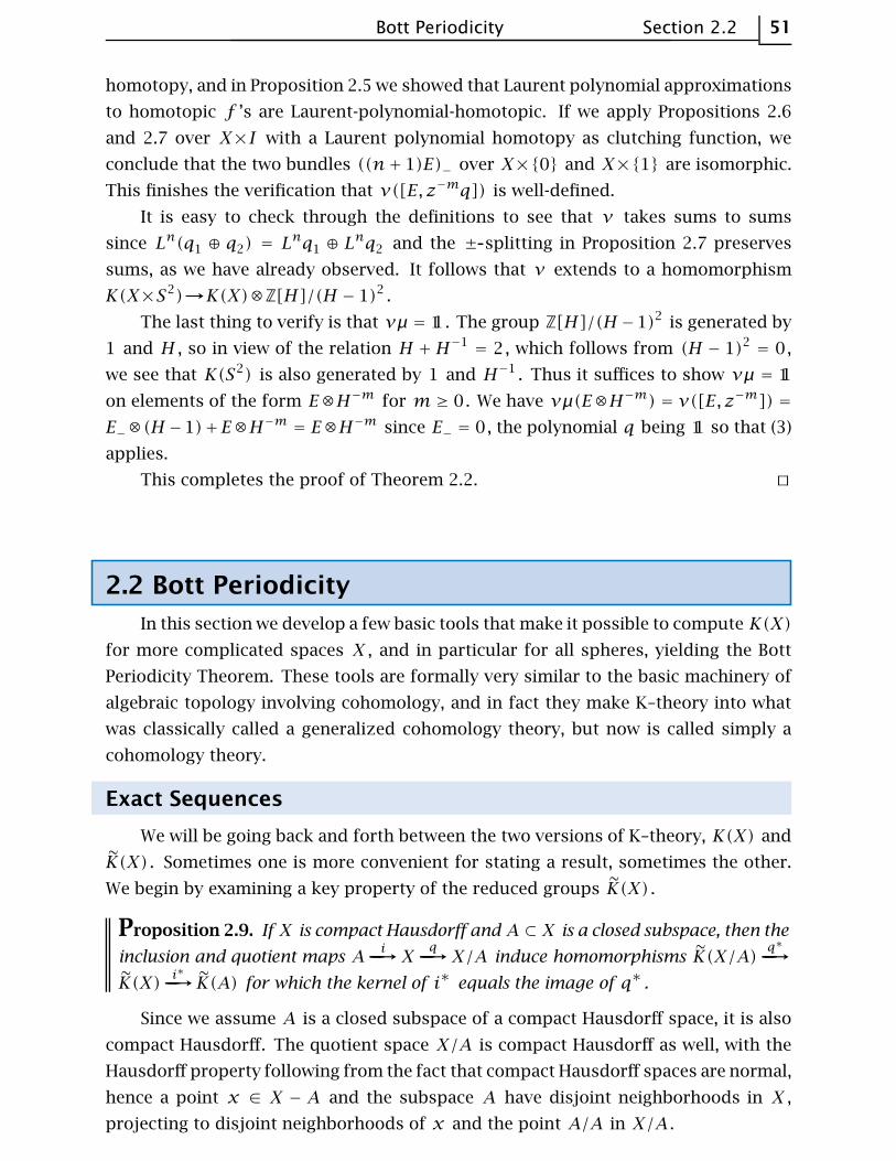
Bott Periodicity Section 2.2 51
homotopy, and in Proposition 2.5 we showed that Laurent polynomial approximations
to homotopic f ’s are Laurent-polynomial-homotopic. If we apply Propositions 2.6
and 2.7 over X×I with a Laurent polynomial homotopy as clutching function, we
conclude that the two bundles ((n+ 1)E)− over X×{0} and X×{1} are isomorphic.
This finishes the verification that ν([E, z−mq]) is well-defined.
It is easy to check through the definitions to see that ν takes sums to sums
since Ln(q1 ⊕ q2) = Lnq1 ⊕ L
nq2 and the ± splitting in Proposition 2.7 preserves
sums, as we have already observed. It follows that ν extends to a homomorphism
K(X×S2)→K(X)⊗Z[H]/(H − 1)2 .
The last thing to verify is that νµ = 11. The group Z[H]/(H −1)2 is generated by
1 and H , so in view of the relation H +H−1 = 2, which follows from (H − 1)2 = 0,
we see that K(S2) is also generated by 1 and H−1 . Thus it suffices to show νµ = 11
on elements of the form E⊗H−m for m ≥ 0. We have νµ(E⊗H−m) = ν([E, z−m]) =
E−⊗(H −1)+E⊗H−m = E⊗H−m since E− = 0, the polynomial q being 11 so that (3)
applies.
This completes the proof of Theorem 2.2. ⊔⊓
2.2 Bott Periodicity
In this section we develop a few basic tools that make it possible to compute K(X)
for more complicated spaces X , and in particular for all spheres, yielding the Bott
Periodicity Theorem. These tools are formally very similar to the basic machinery of
algebraic topology involving cohomology, and in fact they make K–theory into what
was classically called a generalized cohomology theory, but now is called simply a
cohomology theory.
Exact Sequences
We will be going back and forth between the two versions of K–theory, K(X) and
K(X) . Sometimes one is more convenient for stating a result, sometimes the other.
We begin by examining a key property of the reduced groups K(X) .
Proposition 2.9. If X is compact Hausdorff and A ⊂ X is a closed subspace, then the
inclusion and quotient maps Ai-----→X
q-----→X/A induce homomorphisms K(X/A)
q∗
-----→K(X)
i∗
-----→ K(A) for which the kernel of i∗ equals the image of q∗ .
Since we assume A is a closed subspace of a compact Hausdorff space, it is also
compact Hausdorff. The quotient space X/A is compact Hausdorff as well, with the
Hausdorff property following from the fact that compact Hausdorff spaces are normal,
hence a point x ∈ X − A and the subspace A have disjoint neighborhoods in X ,
projecting to disjoint neighborhoods of x and the point A/A in X/A .
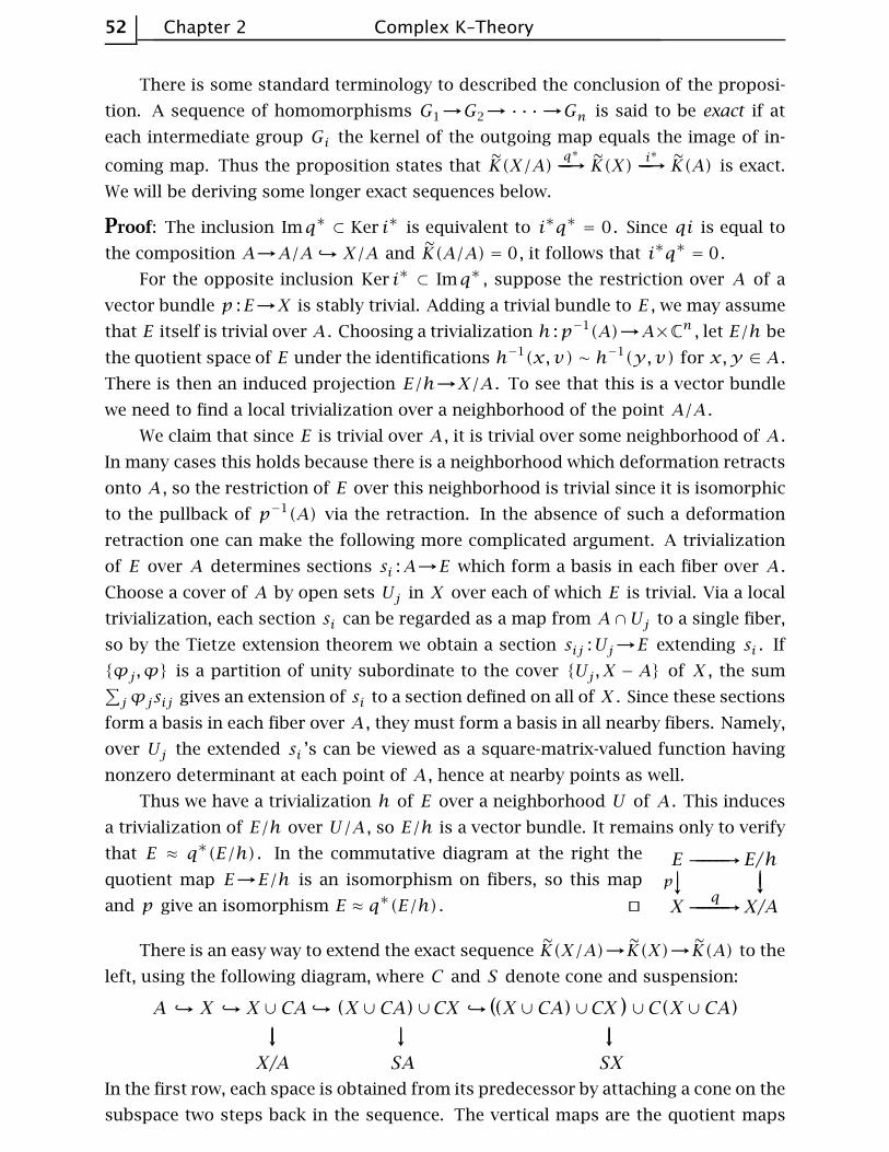
52 Chapter 2 Complex K–Theory
There is some standard terminology to described the conclusion of the proposi-
tion. A sequence of homomorphisms G1→G2→ · · ·→Gn is said to be exact if at
each intermediate group Gi the kernel of the outgoing map equals the image of in-
coming map. Thus the proposition states that K(X/A)q∗
-----→ K(X)i∗
-----→ K(A) is exact.
We will be deriving some longer exact sequences below.
Proof: The inclusion Imq∗ ⊂ Ker i∗ is equivalent to i∗q∗ = 0. Since qi is equal to
the composition A→A/AX/A and K(A/A) = 0, it follows that i∗q∗ = 0.
For the opposite inclusion Ker i∗ ⊂ Imq∗ , suppose the restriction over A of a
vector bundle p :E→X is stably trivial. Adding a trivial bundle to E , we may assume
that E itself is trivial over A . Choosing a trivialization h :p−1(A)→A×Cn , let E/h be
the quotient space of E under the identifications h−1(x,v) ∼ h−1(y,v) for x,y ∈ A .
There is then an induced projection E/h→X/A . To see that this is a vector bundle
we need to find a local trivialization over a neighborhood of the point A/A .
We claim that since E is trivial over A , it is trivial over some neighborhood of A .
In many cases this holds because there is a neighborhood which deformation retracts
onto A , so the restriction of E over this neighborhood is trivial since it is isomorphic
to the pullback of p−1(A) via the retraction. In the absence of such a deformation
retraction one can make the following more complicated argument. A trivialization
of E over A determines sections si :A→E which form a basis in each fiber over A .
Choose a cover of A by open sets Uj in X over each of which E is trivial. Via a local
trivialization, each section si can be regarded as a map from A∩Uj to a single fiber,
so by the Tietze extension theorem we obtain a section sij :Uj→E extending si . If
{ϕj ,ϕ} is a partition of unity subordinate to the cover {Uj , X − A} of X , the sum∑jϕjsij gives an extension of si to a section defined on all of X . Since these sections
form a basis in each fiber over A , they must form a basis in all nearby fibers. Namely,
over Uj the extended si ’s can be viewed as a square-matrix-valued function having
nonzero determinant at each point of A , hence at nearby points as well.
Thus we have a trivialization h of E over a neighborhood U of A . This induces
a trivialization of E/h over U/A , so E/h is a vector bundle. It remains only to verify
that E ≈ q∗(E/h) . In the commutative diagram at the right the
quotient map E→E/h is an isomorphism on fibers, so this map
and p give an isomorphism E ≈ q∗(E/h) . ⊔⊓
There is an easy way to extend the exact sequence K(X/A)→K(X)→K(A) to the
left, using the following diagram, where C and S denote cone and suspension:
In the first row, each space is obtained from its predecessor by attaching a cone on the
subspace two steps back in the sequence. The vertical maps are the quotient maps
Bott Periodicity Section 2.2 53
obtained by collapsing the most recently attached cone to a point. In many cases the
quotient map collapsing a contractible subspace to a point is a homotopy equivalence,
hence induces an isomorphism on K . This conclusion holds generally, in fact:
Lemma 2.10. If A is contractible, the quotient map q :X→X/A induces a bijection
q∗ : Vectn(X/A)→Vectn(X) for all n .
Proof: A vector bundle E→X must be trivial over A since A is contractible. A
trivialization h gives a vector bundle E/h→X/A as in the proof of the previous
proposition. We assert that the isomorphism class of E/h does not depend on h .
This can be seen as follows. Given two trivializations h0 and h1 , by writing h1 =
(h1h−10 )h0 we see that h0 and h1 differ by an element of gx ∈ GLn(C) over each
point x ∈ A . The resulting map g :A→GLn(C) is homotopic to a constant map
x֏ α ∈ GLn(C) since A is contractible. Writing now h1 = (h1h−10 α
−1)(αh0) , we
see that by composing h0 with α in each fiber, which does not change E/h0 , we may
assume that α is the identity. Then the homotopy from g to the identity gives a
homotopy H from h0 to h1 . In the same way that we constructed E/h we construct
a vector bundle (E×I)/H→(X/A)×I restricting to E/h0 over one end and to E/h1
over the other end, hence E/h0 ≈ E/h1 .
Thus we have a well-defined map Vectn(X)→Vectn(X/A) , E֏ E/h . This is an
inverse to q∗ since q∗(E/h) ≈ E as we noted in the preceding proposition, and for a
bundle E→X/A we have q∗(E)/h ≈ E for the evident trivialization h of q∗(E) over
A ⊔⊓
From this lemma and the preceding proposition it follows that we have a long
exact sequence of K groups
· · ·→K(SX)→K(SA)→K(X/A)→K(X)→K(A)
For example, if X is the wedge sum A ∨ B then X/A = B and the sequence breaks
up into split short exact sequences, which implies that the map K(X)→K(A)⊕K(B)obtained by restriction to A and B is an isomorphism.
Deducing Periodicity from the Product Theorem
We can use the exact sequence displayed above to obtain a reduced version of
the external product, a ring homomorphism K(X)⊗K(Y )→K(X ∧Y) where X ∧Y =
X×Y/X ∨ Y and X ∨ Y = X×{y0} ∪ {x0}×Y ⊂ X×Y for chosen basepoints x0 ∈ X
and y0 ∈ Y . The space X ∧ Y is called the smash product of X and Y . To define the
reduced product, consider the long exact sequence for the pair (X×Y ,X ∨ Y) :
54 Chapter 2 Complex K–Theory
The second of the two vertical isomorphisms here was noted earlier. The first vertical
isomorphism arises in similar fashion by using a reduced version of the suspension
operator which associates to a space Z with basepoint z0 the quotient space ΣZof SZ obtained by collapsing the segment {z0}×I to a point. The quotient map
SZ→ΣZ induces an isomorphism K(SZ) ≈ K(ΣZ) by the preceding lemma. For
reduced suspension we have Σ(X ∨Y) = ΣX ∨ΣY , which gives the first isomorphism
in the diagram. The last horizontal map in the sequence is a split surjection, with
splitting K(X)⊕K(Y )→K(X×Y) , (a, b)֏p∗1 (a)+p∗2 (b) where p1 and p2 are the
projections of X×Y onto X and Y . Similarly, the first map splits via (Sp1)∗+(Sp2)
∗ .
So we get a splitting K(X×Y) ≈ K(X ∧ Y)⊕K(X)⊕K(Y ) .
For a ∈ K(X) = Ker(K(X)→K(x0)) and b ∈ K(Y ) = Ker(K(Y)→K(y0)) the
external product a ∗ b = p∗1 (a)p∗2 (b) ∈ K(X×Y) has p∗1 (a) restricting to zero in
K(Y) and p∗2 (b) restricting to zero in K(X) , so p∗1 (a)p∗2 (b) restricts to zero in both
K(X) and K(Y) , hence in K(X ∨ Y) . In particular, a ∗ b lies in K(X×Y) , and from
the short exact sequence above, a ∗ b pulls back to a unique element of K(X ∧ Y) .
This defines the reduced external product K(X)⊗ K(Y )→K(X ∧ Y) . It is essentially
a restriction of the unreduced external product, as shown in the following diagram,
so the reduced external product is also a ring homomorphism, and we shall use the
same notation a ∗ b for both reduced and unreduced external product, leaving the
reader to determine from context which is meant.
Since Sn∧X is the n fold iterated reduced suspension ΣnX , which is a quotient
of the ordinary n fold suspension SnX obtained by collapsing an n disk in SnX to a
point, the quotient map SnX→Sn∧X induces an isomorphism on K by Lemma 2.10.
Then the reduced external product gives rise to a homomorphism
β : K(X)→K(S2X), β(a) = (H − 1)∗ a
where H is the canonical line bundle over S2 = CP1 . Here at last is the Bott Periodicity
Theorem:
Theorem 2.11. The homomorphism β : K(X)→K(S2X) , β(a) = (H − 1)∗ a , is an
isomorphism for all compact Hausdorff spaces X .
Proof: The map β is the composition
K(X) -→K(S2)⊗K(X) -→ K(S2X)
where the first map a֏ (H − 1)⊗a is an isomorphism since K(S2) is infinite cyclic
generated by H − 1, and the second map is the reduced external product, so the
fact that this is an isomorphism is equivalent to the Product Theorem proved in the
previous section, by the diagram displayed above. ⊔⊓
Bott Periodicity Section 2.2 55
Corollary 2.12. K(S2n+1) = 0 and K(S2n) ≈ Z , generated by the n fold reduced
external product (H − 1)∗ · · · ∗ (H − 1) .
Extending to a Cohomology Theory
As we saw earlier, a pair (X,A) of compact Hausdorff spaces gives rise to an exact
sequence of K groups, the first row in the following diagram:
If we set K−n(X) = K(SnX) and K−n(X,A) = K(Sn(X/A)) , this sequence can be
written as in the second row. Negative indices are chosen here so that the ‘coboundary’
maps in this sequence increase dimension, as in ordinary cohomology. The lower
left corner of the diagram containing the Bott periodicity isomorphisms β commutes
since external tensor product with H−1 commutes with maps between spaces. So the
long exact sequence in the second row can be rolled up into a six-term periodic exact
sequence. It is reasonable to extend the definition of Kn to positive n by setting
K2i(X) = K(X) and K2i+1(X) = K(SX) . Then the six-term exact sequence can be
written
A product Ki(X)⊗Kj(Y )→Ki+j(X ∧ Y) is obtained from the external product
K(X)⊗ K(Y )→K(X∧Y) by replacing X and Y by SiX and SjY . If we define K∗(X) =
K0(X)⊕K1(X) , then this gives a product K∗(X)⊗K∗(Y )→K∗(X ∧ Y) . The relative
form of this is a product K∗(X,A)⊗K∗(Y , B)→K∗(X×Y ,X×B∪A×Y) , coming from
the products K(Σi(X/A))⊗K(Σj(Y/B)) -→ K(Σi+j(X/A ∧ Y/B)) using the natural
identification (X×Y)/(X×B ∪A×Y) = X/A∧ Y/B .
If we compose the external product K∗(X)⊗ K∗(X)→K∗(X ∧ X) with the map
K∗(X ∧ X)→K∗(X) induced by the diagonal map X→X ∧ X , x֏ (x,x) , then we
obtain a multiplication on K∗(X) making it into a ring, and it is not hard to check that
this extends the previously defined ring structure on K0(X) . The general relative form
of this product on K∗(X) is a product K∗(X,A)⊗ K∗(X, B)→K∗(X,A∪ B) which is
induced by the relativized diagonal map X/(A∪ B)→X/A∧X/B .
Example 2.13. Suppose that X = A ∪ B where A and B are compact contractible
subspaces of X containing the basepoint. Then the product K∗(X)⊗ K∗(X)→K∗(X)is identically zero since it is equivalent to the composition
K∗(X,A)⊗K∗(X, B)→K∗(X,A∪ B)→K∗(X)
56 Chapter 2 Complex K–Theory
and K∗(X,A∪B) = 0 since X = A∪B . For example if X is a suspension we can take A
and B to be its two cones, with a basepoint in their intersection. As a particular case we
see that the product in K∗(Sn) ≈ Z is trivial for n > 0. For n = 0 the multiplication
in K∗(S0) ≈ Z is just the usual multiplication of integers since Rm⊗Rn ≈ Rmn . This
illustrates the necessity of the condition that A and B both contain the basepoint of
X , since without this condition we could take A and B to be the two points of S0 .
More generally, if X is the union of compact contractible subspaces A1, · · · , Ancontaining the basepoint then the n fold product
K∗(X,A1)⊗ · · · ⊗K∗(X,An)→K∗(X,A1 ∪ · · · ∪An)
is trivial, so all n fold products in K∗(X) are trivial. In particular all elements of
K∗(X) are nilpotent since their nth power is zero. This applies to all compact mani-
folds for example since they are covered by finitely many closed balls, and the condi-
tion that each Ai contain the basepoint can be achieved by adjoining to each ball an
arc to a fixed basepoint. In a similar fashion one can see that this observation applies
to all finite cell complexes, by induction on the number of cells.
Whereas multiplication in K(X) is commutative, in K∗(X) this is only true up to
sign:
Proposition 2.14. αβ = (−1)ijβα for α ∈ Ki(X) and β ∈ Kj(X) .
Proof: The product is the composition
K(Si ∧ X)⊗K(Sj ∧ X) -→ K(Si ∧ Sj ∧X ∧X) -→ K(Si ∧ Sj ∧ X)
where the first map is external product and the second is induced by the diagonal
map on the X factors. Replacing the product αβ by the product βα amounts to
switching the two factors in the first term K(Si∧X)⊗K(Sj∧X) , and this corresponds
to switching the Si and Sj factors in the third term K(Si ∧ Sj ∧X) . Viewing Si ∧ Sj
as the smash product of i + j copies of S1 , then switching Si and Sj in Si ∧ Sj is
a product of ij transpositions of adjacent factors. Transposing the two factors of
S1∧S1 is equivalent to reflection of S2 across an equator. Thus it suffices to see that
switching the two ends of a suspension SY induces multiplication by −1 in K(SY) .
If we view K(SY) as [Y ,U] where U is the infinite unitary group, the union of the
groups U(n) , then switching ends of SY corresponds to the map U→U sending a
matrix to its inverse. By the argument in Example 1.13 the group operation in K(SY)
is the same as the operation induced by the product in U , so the result follows. ⊔⊓
Proposition 2.15. The exact sequence at the right is an
exact sequence of K∗(X) modules, with the maps homo-
morphisms of K∗(X) modules.
Bott Periodicity Section 2.2 57
The K∗(X) module structure on K∗(A) is defined by ξ·α = i∗(ξ)α where i is the
inclusion A X and the product on the right side of the equation is multiplication
in the ring K∗(A) . To define the module structure on K∗(X,A) , observe that the
diagonal map X→X ∧ X induces a well-defined quotient map X/A→X ∧ X/A , and
this leads to a product K∗(X)⊗K∗(X,A)→K∗(X,A) .
Proof: To see that the maps in the exact sequence are module homomorphisms we
look at the diagram
where the vertical maps between the first two rows are external product with a fixed
element of K(SiX) and the vertical maps between the second and third rows are
induced by diagonal maps. What we must show is that the diagram commutes. For the
upper two rows this follows from naturality of external product since the horizontal
maps are induced by maps between spaces. The lower two rows are induced from
suspensions of maps between spaces,
so it suffices to show this diagram commutes up to homotopy. This is obvious for the
middle and right squares. The left square can be rewritten
where the horizontal maps collapse the copy of X in X∪CA to a point, the left vertical
map sends (a, s) ∈ SA to (a,a, s) ∈ X ∧ SA , and the right vertical map sends x ∈ X
to (x,x) ∈ X ∪ CA and (a, s) ∈ CA to (a,a, s) ∈ X ∧ CA . Commutativity is then
obvious. ⊔⊓
It is often convenient to have an unreduced version of the groups Kn(X) , and this
can easily be done by the simple device of defining Kn(X) to be Kn(X+) where X+ is
X with a disjoint basepoint labeled ‘+’ adjoined. For n = 0 this is consistent with the
relation between K and K since K0(X) = K0(X+) = K(X+) = Ker(K(X+)→K(+)) =K(X) . For n = 1 this definition yields K1(X) = K1(X) since S(X+) ≃ SX ∨ S
1 and
K(SX∨S1) ≈ K(SX)⊕K(S1) ≈ K(SX) since K(S1) = 0. For a pair (X,A) with A ≠∅
one defines Kn(X,A) = Kn(X,A) , and then the six-term long exact sequence is valid
58 Chapter 2 Complex K–Theory
also for unreduced groups. When A = ∅ this remains valid if we interpret X/∅ as
X+ .
Since X+∧Y+ = (X×Y)+ , the external product K∗(X)⊗ K∗(Y )→K∗(X∧Y) gives
a product K∗(X)⊗K∗(Y )→K∗(X×Y) . Taking X = Y and composing with the map
K∗(X×X)→K∗(X) induced by the diagonal map X→X×X , x֏ (x,x) , we get a
product K∗(X)⊗K∗(X)→K∗(X) which makes K∗(X) into a ring.
There is a relative product Ki(X,A)⊗Kj(Y , B)→Ki+j(X×Y ,X×B ∪ A×Y) de-
fined as the external product K(Σi(X/A))⊗K(Σj(Y/B)) -→ K(Σi+j(X/A∧ Y/B)) , us-
ing the natural identification (X×Y)/(X×B ∪A×Y) = X/A∧ Y/B . This works when
A = ∅ since we interpret X/∅ as X+ , and similarly if Y = ∅ . Via the diagonal map
we obtain also a product Ki(X,A)⊗Kj(X, B)→Ki+j(X,A∪ B) .With these definitions the preceding two propositions are valid also for unreduced
K–groups.
Division Algebras Section 2.3 59
2.3. Division Algebras and Parallelizable Spheres
With the hard work of proving Bott Periodicity now behind us, the goal of this
section is to prove Adams’ theorem on the Hopf invariant, with its famous applications
including the nonexistence of division algebras beyond the Cayley octonions:
Theorem 2.16. The following statements are true only for n = 1 , 2 , 4 , and 8 :
(a) Rn is a division algebra.
(b) Sn−1 is parallelizable, i.e., there exist n− 1 tangent vector fields to Sn−1 which
are linearly independent at each point, or in other words, the tangent bundle to Sn−1
is trivial.
A division algebra structure on Rn is a multiplication map R
n×Rn→Rn such
that the maps x֏ax and x֏xa are linear for each a ∈ Rn and invertible if a ≠ 0.
Since we are dealing with linear maps Rn→Rn , invertibility is equivalent to having
trivial kernel, which translates into the statement that the multiplication has no zero
divisors. An identity element is not assumed, but the multiplication can be modified
to produce an identity in the following way. Choose a unit vector e ∈ Rn . After
composing the multiplication with an invertible linear map Rn→R
n taking e2 to e
we may assume that e2 = e . Let α be the map x֏xe and β the map x֏ex . The new
product (x,y)֏α−1(x)β−1(y) then sends (x, e) to α−1(x)β−1(e) = α−1(x)e = x ,
and similarly it sends (e,y) to y . Since the maps x֏ax and x֏xa are surjective
for each a ≠ 0, the equations ax = e and xa = e are solvable, so nonzero elements
of the division algebra have multiplicative inverses on the left and right.
H-Spaces
The first step in the proof of the theorem is to reduce it to showing when the
sphere Sn−1 is an H–space.
To say that Sn−1 is an H–space means there is a continuous multiplication map
Sn−1×Sn−1→Sn−1 having a two-sided identity element e ∈ Sn−1 . This is weaker than
being a topological group since associativity and inverses are not assumed. For exam-
ple, S1 , S3 , and S7 are H–spaces by restricting the multiplication of complex numbers,
quaternions, and Cayley octonions to the respective unit spheres, but only S1 and S3
are topological groups since the multiplication of octonions is nonassociative.
Lemma 2.17. If Rn is a division algebra, or if Sn−1 is parallelizable, then Sn−1 is
an H–space.
Proof: Having a division algebra structure on Rn with two-sided identity, an H–space
structure on Sn−1 is given by (x,y)֏xy/|xy| , which is well-defined since a division
algebra has no zero divisors.
Now suppose that Sn−1 is parallelizable, with tangent vector fields v1, · · · , vn−1
which are linearly independent at each point of Sn−1 . By the Gram-Schmidt process we
60 Chapter 2 Complex K–Theory
may make the vectors x,v1(x), · · · , vn−1(x) orthonormal for all x ∈ Sn−1 . We may
assume also that at the first standard basis vector e1 , the vectors v1(e1), · · · , vn−1(e1)
are the standard basis vectors e2, · · · , en , by changing the sign of vn−1 if necessary
to get orientations right, then deforming the vector fields near e1 . Let αx ∈ SO(n)
send the standard basis to x,v1(x), · · · , vn−1(x) . Then the map (x,y)֏ αx(y)
defines an H–space structure on Sn−1 with identity element the vector e1 since αe1
is the identity map and αx(e1) = x for all x . ⊔⊓
Before proceeding further let us list a few easy consequences of Bott periodicity
which will be needed.
(1) We have already seen that K(Sn) is Z for n even and 0 for n odd. This comes
from repeated application of the periodicity isomorphism K(X) ≈ K(S2X) , α֏α∗ (H −1) , the external product with the generator H −1 of K(S2) , where H is
the canonical line bundle over S2 = CP1 . In particular we see that a generator of
K(S2k) is the k fold external product (H − 1)∗ · · ·∗ (H − 1) . We note also that
the multiplication in K(S2k) is trivial since this ring is the k fold tensor product
of the ring K(S2) , which has trivial multiplication by Corollary 2.3.
(2) The external product K(S2k)⊗ K(X)→K(S2k ∧ X) is an isomorphism since it is
an iterate of the periodicity isomorphism.
(3) The external product K(S2k)⊗K(X)→K(S2k×X) is an isomorphism. This fol-
lows from (2) by the same reasoning which showed the equivalence of the reduced
and unreduced forms of Bott periodicity. Since external product is a ring homo-
morphism, the isomorphism K(S2k ∧X) ≈ K(S2k)⊗ K(X) is a ring isomorphism.
For example, since K(S2k) can be described as the quotient ring Z[α]/(α2) , we
can deduce that K(S2k×S2ℓ) is Z[α,β]/(α2, β2) where α and β are the pullbacks
of generators of K(S2k) and K(S2ℓ) under the projections of S2k×S2ℓ onto its
two factors. An additive basis for K(S2k×S2ℓ) is thus {1, α, β,αβ} .
We can apply the last calculation to show that S2k is not an H–space if k > 0.
Suppose µ :S2k×S2k→S2k is an H–space multiplication. The induced homomor-
phism of K–rings then has the form µ∗ :Z[γ]/(γ2)→Z[α,β]/(α2, β2) . We claim that
µ∗(γ) = α+β+mαβ for some integer m . The composition S2k i-----→S2k×S2k µ
-----→S2k
is the identity, where i is the inclusion onto either of the subspaces S2k×{e} or
{e}×S2k , with e the identity element of the H–space structure. The map i∗ for i the
inclusion onto the first factor sends α to γ and β to 0, so the coefficient of α in µ∗(γ)
must be 1. Similarly the coefficient of β must be 1, proving the claim. However, this
leads to a contradiction since it implies that µ∗(γ2) = (α + β +mαβ)2 = 2αβ ≠ 0,
which is impossible since γ2 = 0.
There remains the much more difficult problem of showing that Sn−1 is not an
H–space when n is even and different from 2, 4, and 8. The first step is a simple
construction which associates to a map g :Sn−1×Sn−1→Sn−1 a map g :S2n−1→Sn .
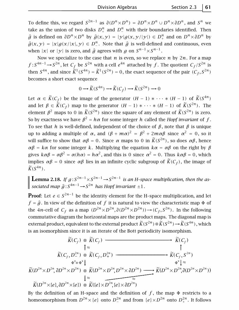
Division Algebras Section 2.3 61
To define this, we regard S2n−1 as ∂(Dn×Dn) = ∂Dn×Dn ∪ Dn×∂Dn , and Sn we
take as the union of two disks Dn+ and Dn− with their boundaries identified. Then
g is defined on ∂Dn×Dn by g(x,y) = |y|g(x,y/|y|) ∈ Dn+ and on Dn×∂Dn by
g(x,y) = |x|g(x/|x|, y) ∈ Dn− . Note that g is well-defined and continuous, even
when |x| or |y| is zero, and g agrees with g on Sn−1×Sn−1 .
Now we specialize to the case that n is even, so we replace n by 2n . For a map
f :S4n−1→S2n , let Cf be S2n with a cell e4n attached by f . The quotient Cf /S2n is
then S4n , and since K1(S4n) = K1(S2n) = 0, the exact sequence of the pair (Cf , S2n)
becomes a short exact sequence
0 -→K(S4n) -→ K(Cf ) -→ K(S2n) -→0
Let α ∈ K(Cf ) be the image of the generator (H − 1) ∗ · · · ∗ (H − 1) of K(S4n)
and let β ∈ K(Cf ) map to the generator (H − 1) ∗ · · · ∗ (H − 1) of K(S2n) . The
element β2 maps to 0 in K(S2n) since the square of any element of K(S2n) is zero.
So by exactness we have β2 = hα for some integer h called the Hopf invariant of f .
To see that h is well-defined, independent of the choice of β , note that β is unique
up to adding a multiple of α , and (β +mα)2 = β2 + 2mαβ since α2 = 0, so it
will suffice to show that αβ = 0. Since α maps to 0 in K(S2n) , so does αβ , hence
αβ = kα for some integer k . Multiplying the equation kα = αβ on the right by β
gives kαβ = αβ2 = α(hα) = hα2 , and this is 0 since α2 = 0. Thus kαβ = 0, which
implies αβ = 0 since αβ lies in an infinite cyclic subgroup of K(Cf ) , the image of
K(S4n) .
Lemma 2.18. If g :S2n−1×S2n−1→S2n−1 is an H–space multiplication, then the as-
sociated map g :S4n−1→S2n has Hopf invariant ±1 .
Proof: Let e ∈ S2n−1 be the identity element for the H–space multiplication, and let
f = g . In view of the definition of f it is natural to view the characteristic map Φ of
the 4n cell of Cf as a map (D2n×D2n, ∂(D2n×D2n))→(Cf , S2n) . In the following
commutative diagram the horizontal maps are the product maps. The diagonal map is
external product, equivalent to the external product K(S2n)⊗ K(S2n)→K(S4n) , which
is an isomorphism since it is an iterate of the Bott periodicity isomorphism.
By the definition of an H–space and the definition of f , the map Φ restricts to a
homeomorphism from D2n×{e} onto D2n− and from {e}×D2n onto D2n
+ . It follows
62 Chapter 2 Complex K–Theory
that the element β⊗β in the upper left group maps to a generator of the group in the
bottom row of the diagram, since β restricts to a generator of K(S2n) by definition.
Therefore by commutativity of the diagram, the product map in the top row sends
β⊗β to ±α since α was defined to be the image of a generator of K(Cf , S2n) . Thus
we have β2 = ±α , which says that the Hopf invariant of f is ±1. ⊔⊓
In view of this lemma, Theorem 2.16 becomes a consequence of the following
theorem of Adams:
Theorem 2.19. There exists a map f :S4n−1→S2n of Hopf invariant ±1 only when
n = 1 , 2 , or 4 .
The proof of this will occupy the rest of this section. The argument will in fact
rule out maps whose Hopf invariant is any odd number when n 6= 1,2,4.
Adams Operations
The Hopf invariant is defined in terms of the ring structure in K–theory, but in
order to prove Adams’ theorem, more structure is needed, namely certain ring homo-
morphisms ψk :K(X)→K(X) . Here are their basic properties:
Theorem 2.20. There exist ring homomorphisms ψk :K(X)→K(X) , defined for all
compact Hausdorff spaces X and all integers k ≥ 0 , and satisfying:
(1) ψkf∗ = f∗ψk for all maps f :X→Y . (Naturality)
(2) ψk(L) = Lk if L is a line bundle.
(3) ψk ◦ψℓ = ψkℓ .
(4) ψp(α) ≡ αp mod p for p prime.
This last statement means that ψp(α)−αp = pβ for some β ∈ K(X) .
In the special case of a vector bundle E which is a sum of line bundles Li , prop-
erties (2) and (3) give the formula ψk(L1⊕ · · · ⊕Ln) = Lk1 + · · · + L
kn . We would like
a general definition of ψk(E) which specializes to this formula when E is a sum of
line bundles. The idea is to use the exterior powers λk(E) . From the corresponding
properties for vector spaces we have:
(i) λk(E1⊕E2) ≈⊕i
(λi(E1)⊗λ
k−i(E2)).
(ii) λ0(E) = 1, the trivial line bundle.
(iii) λ1(E) = E .
(iv) λk(E) = 0 for k greater than the maximum dimension of the fibers of E .
Recall that we want ψk(E) to be Lk1 + · · · + Lkn when E = L1⊕ · · · ⊕Ln for line
bundles Li . We will show in this case that there is a polynomial sk with integer
coefficients such that Lk1+· · ·+Lkn = sk(λ
1(E), · · · , λk(E)) . This will lead us to define
ψk(E) = sk(λ1(E), · · · , λk(E)) for an arbitrary vector bundle E .
Division Algebras Section 2.3 63
To see what the polynomial sk should be, we first use the exterior powers λi(E)
to define a polynomial λt(E) =∑i λi(E)ti ∈ K(X)[t] . This is a finite sum by property
(iv), and property (i) says that λt(E1⊕E2) = λt(E1)λt(E2) . When E = L1⊕ · · · ⊕Lnthis implies that λt(E) =
∏iλt(Li) , which equals
∏i(1 + Lit) by (ii), (iii), and (iv).
The coefficient λj(E) of tj in λt(E) =∏i(1 + Lit) is the j th elementary symmetric
function σj of the Li ’s, the sum of all products of j distinct Li ’s. Thus we have
(∗) λj(E) = σj(L1, · · · , Ln) if E = L1⊕ · · · ⊕Ln
To make the discussion completely algebraic, let us introduce the variable ti for
Li . Thus (1+t1) · · · (1+tn) = 1+σ1+· · ·+σn , where σj is the j th elementary sym-
metric polynomial in the ti ’s. The fundamental theorem on symmetric polynomials,
proved for example in [Lang, p. 134] or [van der Waerden, §26], asserts that every de-
gree k symmetric polynomial in t1, · · · , tn can be expressed as a unique polynomial
in σ1, · · · , σk . In particular, tk1 + · · · + tkn is a polynomial sk(σ1, · · · , σk) , called a
Newton polynomial . This polynomial sk is independent of n since we can pass from
n to n− 1 by setting tn = 0. A recursive formula for sk is
sk = σ1sk−1 − σ2sk−2 + · · · + (−1)k−2σk−1s1 + (−1)k−1kσk
To derive this we may take n = k , and then if we substitute x = −ti in the identity
(x + t1) · · · (x + tk) = xk +σ1x
k−1 + · · ·+σk we get tki = σ1tk−1i − · · · + (−1)k−1σk .
Summing over i then gives the recursion relation. The recursion relation easily yields
for example
s1 = σ1 s2 = σ21 − 2σ2 s3 = σ
31 − 3σ1σ2 + 3σ3
s4 = σ41 − 4σ 2
1σ2 + 4σ1σ3 + 2σ 22 − 4σ4
Summarizing, if we define ψk(E) = sk(λ1(E), · · · , λk(E)) , then in the case that E
is a sum of line bundles L1⊕ · · · ⊕Ln we have
ψk(E) = sk(λ1(E), · · · , λk(E))
= sk(σ1(L1, · · · , Ln), · · · , σk(L1, · · · , Ln)) by (∗)
= Lk1 + · · · + Lkn
Verifying that the definition ψk(E) = sk(λ1(E), · · · , λk(E)) gives operations on
K(X) satisfying the properties listed in the theorem will be rather easy if we make
use of the following general result:
The Splitting Principle. Given a vector bundle E→X with X compact Hausdorff,
there is a compact Hausdorff space F(E) and a map p :F(E)→X such that the in-
duced map p∗ :K∗(X)→K∗(F(E)) is injective and p∗(E) splits as a sum of line
bundles.
This will be proved later in this section, but for the moment let us assume it and
proceed with the proof of Theorem 2.20 and Adams’ theorem.
64 Chapter 2 Complex K–Theory
Proof of Theorem 2.20: Property (1) for vector bundles, f∗(ψk(E)) = ψk(f∗(E)) ,
follows immediately from the relation f∗(λi(E)) = λi(f∗(E)) . Additivity of ψk for
vector bundles, ψk(E1⊕E2) = ψk(E1) +ψ
k(E2) , follows from the splitting principle
since we can first pull back to split E1 then do a further pullback to split E2 , and the
formula ψk(L1⊕ · · · ⊕Ln) = Lk1 + · · · + L
kn preserves sums. Since ψk is additive on
vector bundles, it induces an additive operation on K(X) defined by ψk(E1 − E2) =
ψk(E1)−ψk(E2) .
For this extended ψk the properties (1) and (2) are clear. Multiplicativity is also
easy from the splitting principle: If E is the sum of line bundles Li and E′ is the sum
of line bundles L′j , then E⊗E′ is the sum of the line bundles Li⊗L′j , so ψk(E⊗E′) =
∑i,jψ
k(Li⊗L′j) =
∑i,j(Li⊗L
′j)k =
∑i,j L
ki ⊗L
′jk=∑i Lki
∑j L′jk= ψk(E)ψk(E′) . Thus
ψk is multiplicative for vector bundles, and it follows formally that it is multiplicative
on elements of K(X) . For property (3) the splitting principle and additivity reduce
us to the case of line bundles, where ψk(ψℓ(L)) = Lkℓ = ψkℓ(L) . Likewise for (4), if
E = L1 + · · · + Ln , then ψp(E) = Lp1 + · · · + L
pn ≡ (L1 + · · · + Ln)
p = Ep mod p . ⊔⊓
By the naturality property (1), ψk restricts to an operation ψk : K(X)→K(X) since
K(X) is the kernel of the homomorphism K(X)→K(x0) for x0 ∈ X . For the external
product K(X)⊗ K(Y )→K(X ∧ Y) , we have the formula ψk(α∗ β) = ψk(α) ∗ψk(β)
since if one looks back at the definition of α ∗ β , one sees this was defined as
p∗1 (α)p∗2 (β) , hence
ψk(α∗ β) = ψk(p∗1 (α)p∗2 (β))
= ψk(p∗1 (α))ψk(p∗2 (β))
= p∗1 (ψk(α))p∗2 (ψ
k(β))
= ψk(α)∗ψk(β).
This will allow us to compute ψk on K(S2n) ≈ Z . In this case ψk must be
multiplication by some integer since it is an additive homomorphism of Z .
Proposition 2.21. ψk : K(S2n)→K(S2n) is multiplication by kn .
Proof: Consider first the case n = 1. Since ψk is additive, it will suffice to show
ψk(α) = kα for α a generator of K(S2) . We can take α = H − 1 for H the canonical
line bundle over S2 = CP1 . Then
ψk(α) = ψk(H − 1) = Hk − 1 by property (2)
= (1+α)k − 1
= 1+ kα− 1 since αi = (H − 1)i = 0 for i ≥ 2
= kα
When n > 1 we use the external product K(S2)⊗K(S2n−2)→K(S2n) , which is
an isomorphism, and argue by induction. Assuming the desired formula holds in
Division Algebras Section 2.3 65
K(S2n−2) , we have ψk(α ∗ β) = ψk(α) ∗ψk(β) = kα ∗ kn−1β = kn(α ∗ β) , and we
are done. ⊔⊓
Now we can use the operations ψ2 and ψ3 and the relation ψ2ψ3 = ψ6 = ψ3ψ2
to prove Adams’ theorem.
Proof of Theorem 2.19: The definition of the Hopf invariant of a map f :S4n−1→S2n
involved elements α,β ∈ K(Cf ) . By Proposition 2.21, ψk(α) = k2nα since α is the
image of a generator of K(S4n) . Similarly, ψk(β) = knβ + µkα for some µk ∈ Z .
Therefore
ψkψℓ(β) = ψk(ℓnβ+ µℓα) = knℓnβ+ (k2nµℓ + ℓ
nµk)α
Since ψkψℓ = ψkℓ = ψℓψk , the coefficient k2nµℓ + ℓnµk of α is unchanged when k
and ℓ are switched. This gives the relation
k2nµℓ + ℓnµk = ℓ
2nµk + knµℓ, or (k2n − kn)µℓ = (ℓ
2n − ℓn)µk
By property (4) of ψ2 , we have ψ2(β) ≡ β2 mod 2. Since β2 = hα with h the Hopf
invariant of f , the formula ψ2(β) = 2nβ+ µ2α implies that µ2 ≡ h mod 2, so µ2 is
odd if we assume h is ±1 or any odd number. By the preceding displayed formula
we have (22n − 2n)µ3 = (32n − 3n)µ2 , or 2n(2n − 1)µ3 = 3n(3n − 1)µ2 , so 2n divides
3n(3n − 1)µ2 . Since 3n and µ2 are odd, 2n must then divide 3n − 1. The proof is
completed by the following elementary number theory fact. ⊔⊓
Lemma 2.22. If 2n divides 3n − 1 then n = 1,2 , or 4 .
Proof: Write n = 2ℓm with m odd. We will show that the highest power of 2 dividing
3n − 1 is 2 for ℓ = 0 and 2ℓ+2 for ℓ > 0. This implies the lemma since if 2n divides
3n−1, then by this fact, n ≤ ℓ+2, hence 2ℓ ≤ 2ℓm = n ≤ ℓ+2, which implies ℓ ≤ 2
and n ≤ 4. The cases n = 1,2,3,4 can then be checked individually.
We find the highest power of 2 dividing 3n − 1 by induction on ℓ . For ℓ = 0
we have 3n − 1 = 3m − 1 ≡ 2 mod 4 since 3 ≡ −1 mod 4 and m is odd. In the next
case ℓ = 1 we have 3n − 1 = 32m − 1 = (3m − 1)(3m + 1) . The highest power of 2
dividing the first factor is 2 as we just showed, and the highest power of 2 dividing
the second factor is 4 since 3m + 1 ≡ 4 mod 8 because 32 ≡ 1 mod 8 and m is
odd. So the highest power of 2 dividing the product (3m − 1)(3m + 1) is 8. For the
inductive step of passing from ℓ to ℓ + 1 with ℓ ≥ 1, or in other words from n to
2n with n even, write 32n − 1 = (3n − 1)(3n + 1) . Then 3n + 1 ≡ 2 mod 4 since n
is even, so the highest power of 2 dividing 3n + 1 is 2. Thus the highest power of 2
dividing 32n − 1 is twice the highest power of 2 dividing 3n − 1. ⊔⊓
66 Chapter 2 Complex K–Theory
The Splitting Principle
The splitting principle will be a fairly easy consequence of a general result about
the K–theory of fiber bundles called the Leray-Hirsch theorem, together with a calcu-
lation of the ring structure of K∗(CPn) . The following proposition will allow us to
compute at least the additive structure of K∗(CPn) .
Proposition 2.23. If X is a finite cell complex with n cells, then K∗(X) is a finitely
generated group with at most n generators. If all the cells of X have even dimension
then K1(X) = 0 and K0(X) is free abelian with one basis element for each cell.
The phrase ‘finite cell complex’ would normally mean ‘finite CW complex’ but we
can take it to be something slightly more general: a space built from a finite discrete set
by attaching a finite number of cells in succession, with no conditions on the dimen-
sions of these cells, so cells are not required to attach only to cells of lower dimension.
Finite cell complexes are always homotopy equivalent to finite CW complexes (by de-
forming each successive attaching map to be cellular) so the only advantages of finite
cell complexes are technical. In particular, it is easy to see that a space is a finite cell
complex if it is a fiber bundle over a finite cell complex with fibers that are also finite
cell complexes. This is shown in Proposition 2.28 in a brief appendix to this section.
It implies that the splitting principle can be applied staying within the realm of finite
cell complexes.
Proof: We show this by induction on the number of cells. The complex X is obtained
from a subcomplex A by attaching a k cell, for some k . For the pair (X,A) we
have an exact sequence K∗(X/A) -→ K∗(X) -→ K∗(A) . Since X/A = Sk , we have
K∗(X/A) ≈ Z , and exactness implies that K∗(X) requires at most one more generator
than K∗(A) .
The first term of the exact sequence K1(X/A)→K1(X)→K1(A) is zero if all
cells of X are of even dimension, so induction on the number of cells implies that
K1(X) = 0. Then there is a short exact sequence 0→K0(X/A)→K0(X)→K0(A)→0
with K0(X/A) ≈ Z . By induction K(A) is free, so this sequence splits, hence K0(X) ≈
Z⊕K0(A) and the final statement of the proposition follows. ⊔⊓
This proposition applies in particular to CPn , which has a cell structure with one
cell in each dimension 0,2,4, · · · ,2n , so K1(CPn) = 0 and K0(CPn) ≈ Zn+1 . The ring
structure is as simple as one could hope for:
Proposition 2.24. K(CPn) is the quotient ring Z[L]/(L−1)n+1 where L is the canon-
ical line bundle over CPn .
Thus by the change of variable x = L−1 we see that K(CPn) is the truncated poly-
nomial ring Z[x]/(xn+1) , with additive basis 1, x, · · · , xn . It follows that 1, L, · · · , Ln
is also an additive basis.
Division Algebras Section 2.3 67
Proof: The exact sequence for the pair (CPn,CPn−1) gives a short exact sequence
0 -→K(CPn,CPn−1) -→K(CPn)ρ-----→K(CPn−1) -→0
We shall prove:
(an) (L− 1)n generates the kernel of the restriction map ρ .
Hence if we assume inductively that K(CPn−1) = Z[L]/(L − 1)n , then (an) and the
preceding exact sequence imply that {1, L− 1, · · · , (L − 1)n} is an additive basis for
K(CPn) . Since (L − 1)n+1 = 0 in K(CPn) by (an+1) , it follows that K(CPn) is the
quotient ring Z[L]/(L− 1)n+1 , completing the induction.
A reason one might expect (an) to be true is that the kernel of ρ can be identi-
fied with K(CPn,CPn−1) = K(S2n) by the short exact sequence, and Bott periodicity
implies that the n fold reduced external product of the generator L − 1 of K(S2)
with itself generates K(S2n) . To make this rough argument into a proof we will have
to relate the external product K(S2)⊗ · · · ⊗ K(S2)→K(S2n) to the ‘internal’ product
K(CPn)⊗ · · · ⊗K(CPn)→K(CPn) .
The space CPn is the quotient of the unit sphere S2n+1 in Cn+1 under multipli-
cation by scalars in S1 ⊂ C . Instead of S2n+1 we could equally well take the boundary
of the product D20× · · · ×D
2n where D2
i is the unit disk in the ith coordinate of Cn+1 ,
and we start the count with i = 0 for convenience. Then we have
∂(D20× · · · ×D
2n) =
⋃i(D
20× · · · ×∂D
2i × · · · ×D
2n)
The action of S1 by scalar multiplication respects this decomposition. The orbit space
of D20× · · · ×∂D
2i × · · · ×D
2n under the action is a subspace Ci ⊂ CPn homeomorphic
to the product D20× · · · ×D
2n with the factor D2
i deleted. Thus we have a decompo-
sition CPn =⋃i Ci with each Ci homeomorphic to D2n and with Ci ∩Cj = ∂Ci ∩ ∂Cj
for i ≠ j .
Consider now C0 = D21× · · · ×D
2n . Its boundary is decomposed into the pieces
∂iC0 = D21× · · · ×∂D
2i × · · · ×D
2n . The inclusions (D2
i , ∂D2i ) ⊂ (C0, ∂iC0) ⊂ (CPn, Ci)
give rise to a commutative diagram
where the maps from the first column to the second are the n fold products. The
upper map in the middle column is an isomorphism because the inclusion C0CPn
induces a homeomorphism C0/∂C0 ≈ CPn/(C1∪· · ·∪Cn) . The CPn−1 at the right side
68 Chapter 2 Complex K–Theory
of the diagram sits in CPn in the last n coordinates of Cn+1 , so is disjoint from C0 ,
hence the quotient map CPn/CPn−1→CPn/(C1∪· · ·∪Cn) is a homotopy equivalence.
The element xi ∈ K(CPn, Ci) mapping downward to L−1 ∈ K(CPn) maps upward
to a generator of K(C0, ∂iC0) ≈ K(D2i , ∂D
2i ) . By commutativity of the diagram, the
product x1 · · ·xn then generates K(CPn, C1 ∪ · · · ∪ Cn) . This means that (L − 1)n
generates the image of the map K(CPn,CPn−1)→K(CPn) , which equals the kernel of
ρ , proving (an) . ⊔⊓
Since CPn is the union of the n+1 balls Ci , Example 2.13 shows that all products
of n + 1 elements of K(CPn) must be zero, in particular (L − 1)n+1 = 0. But as we
have just seen, (L− 1)n is nonzero, so the result in Example 2.13 is best possible in
terms of the degree of nilpotency.
Now we come to the Leray-Hirsch theorem for K–theory, which will be the major
theoretical ingredient in the proof of the splitting principle:
Theorem 2.25. Let p :E→B be a fiber bundle with E and B compact Hausdorff and
with fiber F such that K∗(F) is free. Suppose that there exist classes c1, · · · , ck ∈
K∗(E) that restrict to a basis for K∗(F) in each fiber F . If either
(a) B is a finite cell complex, or
(b) F is a finite cell complex having all cells of even dimension,
then K∗(E) , as a module over K∗(B) , is free with basis {c1, · · · , ck} .
Here the K∗(B) module structure on K∗(E) is defined by β · γ = p∗(β)γ for
β ∈ K∗(B) and γ ∈ K∗(E) . Another way to state the conclusion of the theorem is
to say that the map Φ :K∗(B)⊗K∗(F)→K∗(E) , Φ(∑i bi ⊗ i
∗(ci)) =∑i p∗(bi)ci for i
the inclusion F E , is an isomorphism.
In the case of the product bundle E = F×B the classes ci can be chosen to be the
pullbacks under the projection E→F of a basis for K∗(F) . The theorem then asserts
that the external product K∗(F)⊗K∗(B)→K∗(F×B) is an isomorphism.
For most of our applications of the theorem either case (a) or case (b) will suffice.
The proof of (a) is somewhat simpler than (b), and we include (b) mainly to obtain the
splitting principle for vector bundles over arbitrary compact Hausdorff base spaces.
Proof: For a subspace B′ ⊂ B let E′ = p−1(B′) . Then we have a diagram
where the left-hand Φ is defined by the same formula Φ(∑i bi ⊗ i∗(ci)) =∑i p∗(bi)ci ,
but with p∗(bi)ci referring now to the relative product K∗(E, E′)×K∗(E)→K∗(E, E′) .The right-hand Φ is defined using the restrictions of the ci ’s to the subspace E′ . To
see that the diagram (∗) commutes, we can interpolate between its two rows the row
-→K∗(E, E′)⊗K∗(F) -→K∗(E)⊗K∗(F) -→K∗(E′)⊗K∗(F) -→
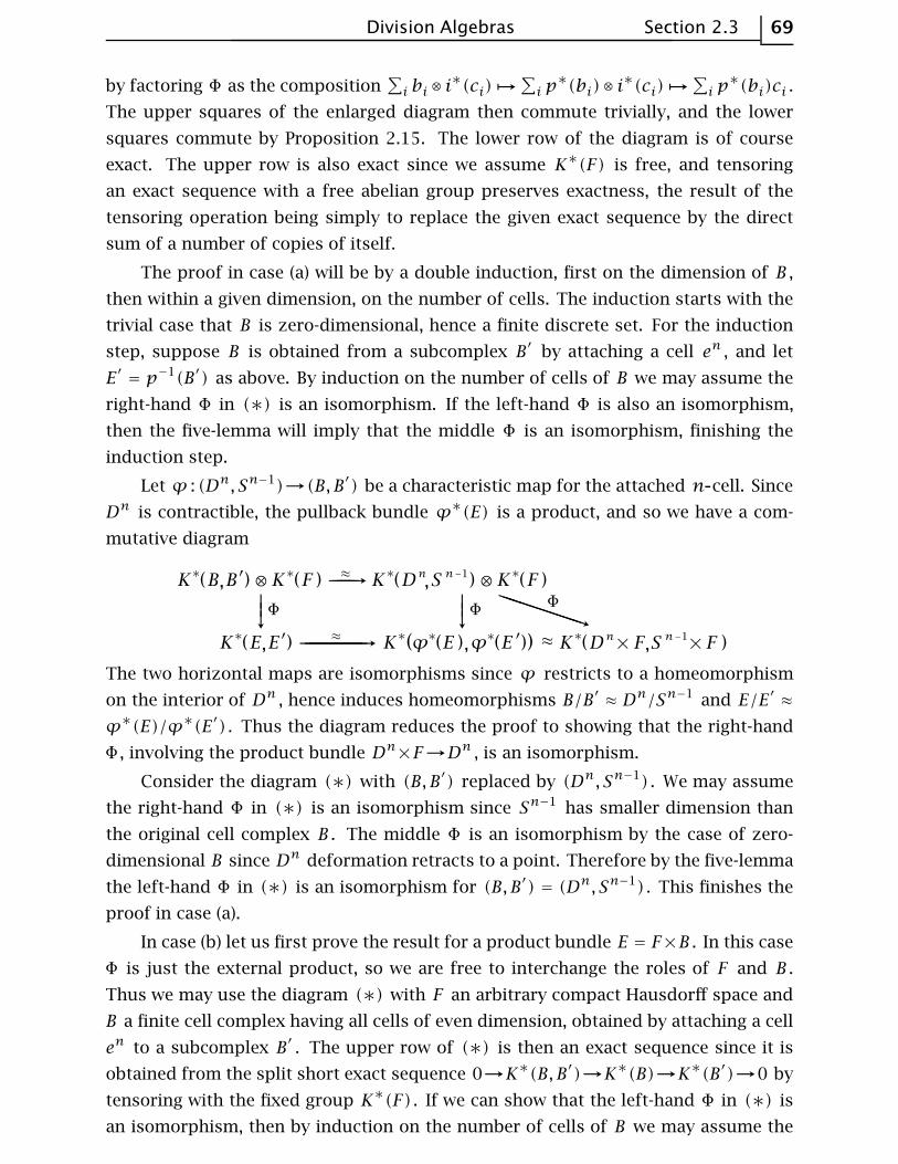
Division Algebras Section 2.3 69
by factoring Φ as the composition∑i bi ⊗ i
∗(ci)֏∑i p∗(bi)⊗ i
∗(ci)֏∑i p∗(bi)ci .
The upper squares of the enlarged diagram then commute trivially, and the lower
squares commute by Proposition 2.15. The lower row of the diagram is of course
exact. The upper row is also exact since we assume K∗(F) is free, and tensoring
an exact sequence with a free abelian group preserves exactness, the result of the
tensoring operation being simply to replace the given exact sequence by the direct
sum of a number of copies of itself.
The proof in case (a) will be by a double induction, first on the dimension of B ,
then within a given dimension, on the number of cells. The induction starts with the
trivial case that B is zero-dimensional, hence a finite discrete set. For the induction
step, suppose B is obtained from a subcomplex B′ by attaching a cell en , and let
E′ = p−1(B′) as above. By induction on the number of cells of B we may assume the
right-hand Φ in (∗) is an isomorphism. If the left-hand Φ is also an isomorphism,
then the five-lemma will imply that the middle Φ is an isomorphism, finishing the
induction step.
Let ϕ : (Dn, Sn−1)→(B, B′) be a characteristic map for the attached n cell. Since
Dn is contractible, the pullback bundle ϕ∗(E) is a product, and so we have a com-
mutative diagram
The two horizontal maps are isomorphisms since ϕ restricts to a homeomorphism
on the interior of Dn , hence induces homeomorphisms B/B′ ≈ Dn/Sn−1 and E/E′ ≈
ϕ∗(E)/ϕ∗(E′) . Thus the diagram reduces the proof to showing that the right-hand
Φ , involving the product bundle Dn×F→Dn , is an isomorphism.
Consider the diagram (∗) with (B, B′) replaced by (Dn, Sn−1) . We may assume
the right-hand Φ in (∗) is an isomorphism since Sn−1 has smaller dimension than
the original cell complex B . The middle Φ is an isomorphism by the case of zero-
dimensional B since Dn deformation retracts to a point. Therefore by the five-lemma
the left-hand Φ in (∗) is an isomorphism for (B, B′) = (Dn, Sn−1) . This finishes the
proof in case (a).
In case (b) let us first prove the result for a product bundle E = F×B . In this case
Φ is just the external product, so we are free to interchange the roles of F and B .
Thus we may use the diagram (∗) with F an arbitrary compact Hausdorff space and
B a finite cell complex having all cells of even dimension, obtained by attaching a cell
en to a subcomplex B′ . The upper row of (∗) is then an exact sequence since it is
obtained from the split short exact sequence 0→K∗(B, B′)→K∗(B)→K∗(B′)→0 by
tensoring with the fixed group K∗(F) . If we can show that the left-hand Φ in (∗) is
an isomorphism, then by induction on the number of cells of B we may assume the
70 Chapter 2 Complex K–Theory
right-hand Φ is an isomorphism, so the five-lemma will imply that the middle Φ is
also an isomorphism.
To show the left-hand Φ is an isomorphism, note first that B/B′ = Sn so we may
as well take the pair (B, B′) to be (Dn, Sn−1) . Then the middle Φ in (∗) is obviously
an isomorphism, so the left-hand Φ will be an isomorphism iff the right-hand Φ is
an isomorphism. When the sphere Sn−1 is even-dimensional we have already shown
that Φ is an isomorphism in the remarks following the proof of Lemma 2.17, and
the same argument applies also when the sphere is odd-dimensional, since K1 of an
odd-dimensional sphere is K0 of an even-dimensional sphere.
Now we turn to case (b) for nonproducts. The proof will once again be inductive,
but this time we need a more subtle inductive statement since B is just a compact
Hausdorff space, not a cell complex. Consider the following condition on a compact
subspace U ⊂ B :
For all compact V ⊂ U the map Φ :K∗(V)⊗K∗(F)→K∗(p−1(V)) is an isomor-
phism.
If this is satisfied, let us call U good. By the special case already proved, each point of
B has a compact neighborhood U that is good. Since B is compact, a finite number
of these neighborhoods cover B , so by induction it will be enough to show that if U1
and U2 are good, then so is U1 ∪ U2 .
A compact V ⊂ U1 ∪ U2 is the union of V1 = V ∩ U1 and V2 = V ∩ U2 . Consider
the diagram like (∗) for the pair (V,V2) . Since K∗(F) is free, the upper row of this
diagram is exact. Assuming U2 is good, the map Φ is an isomorphism for V2 , so Φwill be an isomorphism for V if it is an isomorphism for (V,V2) . The quotient V/V2
is homeomorphic to V1/(V1∩V2) assuming we are not in the trivial case V1∩V2 = ∅ ,
so Φ will be an isomorphism for (V,V2) if it is an isomorphism for (V1, V1∩V2) . Now
look at the diagram like (∗) for (V1, V1 ∩V2) . Assuming U1 is good, the maps Φ are
isomorphisms for V1 and V1∩V2 . Hence Φ is an isomorphism for (V1, V1∩V2) , and
the induction step is finished. ⊔⊓
Example 2.26. Let E→X be a vector bundle with fibers Cn and compact base X .
Then we have an associated projective bundle p :P(E)→X with fibers CPn−1 , where
P(E) is the space of lines in E , that is, one-dimensional linear subspaces of fibers of
E . Over P(E) there is the canonical line bundle L→P(E) consisting of the vectors in
the lines of P(E) . In each fiber CPn−1 of P(E) the classes 1, L, · · · , Ln−1 in K∗(P(E))
restrict to a basis for K∗(CPn−1) by Proposition 2.24. From the Leray-Hirsch theorem
we deduce that K∗(P(E)) is a free K∗(X) module with basis 1, L, · · · , Ln−1 .
Proof of the Splitting Principle: In the preceding example, the fact that 1 is among the
basis elements implies that p∗ :K∗(X)→K∗(P(E)) is injective. The pullback bundle
p∗(E)→P(E) contains the line bundle L as a subbundle, hence splits as L⊕E′ for
E′→P(E) the subbundle of p∗(E) orthogonal to L with respect to some choice of
Division Algebras Section 2.3 71
inner product. Now repeat the process by forming P(E′) , splitting off another line
bundle from the pullback of E′ over P(E′) . Note that P(E′) is the space of pairs
of orthogonal lines in fibers of E . After a finite number of repetitions we obtain
the flag bundle F(E)→X described at the end of §1.1, whose points are n tuples of
orthogonal lines in fibers of E , where n is the dimension of E . (If the fibers of E
have different dimensions over different components of X , we do the construction
for each component separately.) The pullback of E over F(E) splits as a sum of line
bundles, and the map F(E)→X induces an injection on K∗ since it is a composition
of maps with this property. ⊔⊓
In the preceding Example 2.26 we saw that K∗(P(E)) is free as a K∗(X) module,
with basis 1, L, · · · , Ln−1 . In order to describe the multiplication in K∗(P(E)) one
therefore needs only a relation expressing Ln in terms of lower powers of L . Such
a relation can be found as follows. The pullback of E over P(E) splits as L⊕E′ for
some bundle E′ of dimension n− 1, and the desired relation will be λn(E′) = 0. To
compute λn(E′) we use the formula λt(E) = λt(L)λt(E′) in K∗(P(E))[t] , where to
simplify notation we let E also denote the pullback of E over P(E) . The equation
λt(E) = λt(L)λt(E′) can be rewritten as λt(E
′) = λt(E)λt(L)−1 where λt(L)
−1 is the
formal power series∑i(−1)iLiti since λt(L) = 1+ Lt . Equating coefficients of tn in
the two sides of λt(E′) = λt(E)λt(L)
−1 , we get λn(E′) =∑i(−1)n−iλi(E)Ln−i . The
relation λn(E′) = 0 can then be written as∑i(−1)iλi(E)Ln−i = 0, with the coefficient
of Ln equal to 1 as desired. The result can be stated in the following form:
Proposition 2.27. For an n dimensional vector bundle E→X the ring K(P(E)) is
isomorphic to the quotient ring K∗(X)[L]/(∑
i(−1)iλi(E)Ln−i). ⊔⊓
For example when X is a point we have P(E) = CPn−1 and λi(E) = Ck for k =(ni
),
so the polynomial∑i(−1)iλi(E)Ln−i becomes (L−1)n and we see that the proposition
generalizes the isomorphism K∗(CPn−1) ≈ Z[L]/(L− 1)n .
Appendix: Finite Cell Complexes
As we mentioned in the remarks following Proposition 2.23 it is convenient for
purposes of the splitting principle to work with spaces slightly more general than finite
CW complexes. By a finite cell complex we mean a space which has a finite filtration
X0 ⊂ X1 ⊂ · · · ⊂ Xk = X where X0 is a finite discrete set and Xi+1 is obtained from
Xi by attaching a cell eni via a map ϕi :Sni−1→Xi . Thus Xi+1 is the quotient space
of the disjoint union of Xi and a disk Dni under the identifications x ∼ ϕi(x) for
x ∈ ∂Dni = Sni−1 .
Proposition 2.28. If p :E→B is a fiber bundle whose fiber F and base B are both
finite cell complexes, then E is also a finite cell complex, whose cells are products of
cells in B with cells in F .
72 Chapter 2 Complex K–Theory
Proof: Suppose B is obtained from a subcomplex B′ by attaching a cell en . By induc-
tion on the number of cells of B we may assume that p−1(B′) is a finite cell complex.
If Φ :Dn→B is a characteristic map for en then the pullback bundle Φ∗(E)→Dn is
a product since Dn is contractible. Since F is a finite cell complex, this means that
we may obtain Φ∗(E) from its restriction over Sn−1 by attaching cells. Hence we may
obtain E from p−1(B′) by attaching cells. ⊔⊓
Characteristic classes are cohomology classes associated to vector bundles. They
measure in some way how a vector bundle is twisted, or nontrivial. There are four
main kinds:
1. Stiefel-Whitney classes wi(E) ∈ Hi(B;Z2) for a real vector bundle E→B .
2. Chern classes ci(E) ∈ H2i(B;Z) for a complex vector bundle E→B .
3. Pontryagin classes pi(E) ∈ H4i(B;Z) for a real vector bundle E→B .
4. The Euler class e(E) ∈ Hn(B;Z) for an oriented n dimensional real vector bundle
E→B .
The Stiefel-Whitney and Chern classes are formally quite similar. Pontryagin classes
can be regarded as a refinement of Stiefel-Whitney classes when one takes Z rather
than Z2 coefficients, and the Euler class is a further refinement in the orientable case.
For an n dimensional vector bundle E→B to be trivial is equivalent to its clas-
sifying map f :B→Gn being nullhomotopic, but as with most things in homotopy
theory it can be quite difficult to determine whether this is the case or not. Much
more accessible is the weaker question of whether f induces a nontrivial map on ho-
mology or cohomology, and this is precisely what characteristic classes measure. The
Stiefel-Whitney classes wi , like the other characteristic classes, satisfy the important
naturality property that wi(f∗(E)) = f∗(wi(E)) , so in particular if f is a classifying
map B→Gn for E we have E = f∗(En) and wi(E) = wi(f∗(En)) = f
∗(wi(En)) .
Thus if f induces the trivial map on Z2 cohomology, then the Stiefel-Whitney classes
of E are trivial. The converse statement is also true because the classes wi(En) gen-
erate the cohomology ring H∗(Gn;Z2) . In fact H∗(Gn;Z2) is exactly the polynomial
ring Z2[w1(En), · · · ,wn(En)] . This is one reason for considering Z2 rather than Z
coefficients, since H∗(Gn;Z) has a more complicated ring structure, and the Pontrya-
gin classes pi(En) are needed in order to describe it completely. Even though this
description is not so nice, it is nevertheless true that f induces the trivial map on co-
74 Chapter 3 Characteristic Classes
homology with arbitrary coefficients iff all the Stiefel-Whitney and Pontryagin classes
of E are zero. If E is orientable we can take its classifying map to be a map to Gn ,
and the corresponding statement here is that this map induces the trivial map on
cohomology with arbitrary coefficients iff the Euler class of E as well as all its Stiefel-
Whitney and Pontryagin classes are trivial. For complex vector bundles the analogous
statements are also true but somewhat simpler since one only needs Chern classes,
as H∗(Gn(C);Z) is the polynomial ring Z[c1, · · · , cn] on the Chern classes ci of the
universal bundle over Gn(C) .
The vanishing of all the characteristic classes of a vector bundle is a necessary
condition for it to be trivial, but it is not always sufficient, as there exist nontrivial
vector bundles whose characteristic classes are all zero. Perhaps the simplest example
is the tangent bundle of the sphere S5 . One reason why characteristic classes are not
sufficient to determine when a vector bundle is trivial is that, except for the Euler
class, they are stable invariants, meaning that taking the direct sum of a given bundle
with a trivial bundle does not change the characteristic classes. Thus for a vector
bundle which is stably trivial, such as the tangent bundle of a sphere, only the Euler
class has a chance of detecting nontriviality of the bundle. A key feature of the Euler
class is that it is zero for vector bundles that split as the sum of a trivial bundle with
some other bundle. Tangent bundles to odd-dimensional spheres have this property
since they have nonzero sections, splitting off a trivial line bundle. Thus these tangent
bundles have no nonzero characteristic classes, but only S1 , S3 , and S7 have trivial
tangent bundles, as we showed in the previous chapter.
What Exactly Do Characteristic Classes Measure?
Let us see how one might attack the question of what makes a vector bundle non-
trivial. The first obstacle to triviality is orientability. For a vector bundle E→B with
B path-connected, orientability is detected by the homomorphism π1(B)→Z2 that
assigns 0 or 1 to each loop according to whether orientations of fibers are preserved
or reversed as one goes around the loop. Since Z2 is abelian, this homomorphism
factors through the abelianization H1(B) of π1(B) , and homomorphisms H1(B)→Z2
are identifiable with elements of H1(B;Z2) . Thus we have an element of H1(B;Z2)
associated to E which is zero exactly when E is orientable. This is exactly the first
Stiefel-Whitney class w1(E) .
Let us assume now that B is a CW complex. Then E is orientable iff its restriction
to the 1 skeleton B1 of B is orientable, since all loops in B can be deformed to lie
in B1 . Furthermore, a vector bundle over a 1 dimensional CW complex is trivial iff it
is orientable, so we can also say that w1(E) measures whether E is trivial over the
1 skeleton B1 .
Having an understanding of when E is trivial over the 1 skeleton we can ask about
triviality over each successive higher skeleton. Assuming that E is trivial over B1 , then
if the fibers have dimension n we can choose n orthonormal sections over B1 , and
Characteristic Classes 75
so we ask whether these sections extend to orthonormal sections over each 2 cell. If
we pull E back to a vector bundle over the disk D2 via a characteristic map D2→Bfor a 2 cell, the sections over B1 pull back to sections of the pullback over ∂D2 . The
pullback bundle is trivial since D2 is contractible, so by choosing a trivialization the
sections over ∂D2 determine a map ∂D2→O(n) . If we choose the trivialization to
give the same orientation as the trivialization of E over B1 determined by the sections,
we can take this map ∂D2→O(n) to have image in the identity component SO(n) of
O(n) . Thus we have an element of π1(SO(n)) for each 2 cell, and it is not hard to
see that the sections over B1 extend to orthonormal sections over B2 iff this element
of π1(SO(n)) is zero for each 2 cell. The group π1(SO(n)) is obviously 0 for n = 1,
and it is Z for n = 2 since SO(2) is homeomorphic to S1 . For n ≥ 3 it is not hard to
compute that π1(SO(n)) is Z2 , with the obvious inclusion SO(2)SO(n) inducing
a surjection on π1 , so a generator of π1(SO(n)) for n ≥ 2 is represented by the loop
given by rotating a plane through 360 degrees, fixing the orthogonal complement of
this plane. We can regard the function which assigns to each 2 cell the element of
π1(SO(n)) which is the obstruction to extending the sections over the 2 cell as a
2 dimensional cellular cochain with coefficients in π1(SO(n)) . It turns out to be a
cellular cocycle, and so defines an element of H2(B;π1(SO(n))) . This element, call
it ω2(E) , does not depend on the original choice of the sections over B1 , and by
rechoosing these sections if necessary one can see that E is trivial over B2 iff ω2(E)
is zero in H2(B;π1(SO(n))) . When n = 1 we have ω2(E) = 0 automatically, so E is
trivial over B2 in this case. When n = 2 the class ω2(E) lies in H2(B;Z) and equals
the Euler class e(E) . For n ≥ 3 we have ω2(E) lying in H2(B;Z2) and it equals the
Stiefel-Whitney class w2(E) . (When n = 2, w2(E) is the image of e(E) under the
homomorphism H2(B;Z)→H2(B;Z2) reducing coefficients mod 2.)
If E is trivial over B2 we can try to extend n orthonormal sections from B2 to
B3 in the same way, cell by cell. For each cell the obstruction to extending lies in
π2(SO(n)) . This group happens to be zero for all n , so the sections automatically
extend over B3 . At the next step we seek to extend over 4 cells, where the obstructions
lie in π3(SO(n)) . These groups can also be computed explicitly with only a little more
effort than for π1 and π2 , and they are 0 for n ≤ 2, Z for n = 3, Z⊕Z for n = 4,
and Z again for n ≥ 5. By reasoning analogous to that for 2 cells we then obtain an
obstruction ω4(E) ∈ H4(B;π3(SO(n))) . In the cases when the coefficient group is
Z this turns out to be the Pontryagin class p1(E) . In the special case n = 4 when
π3(SO(4)) is Z⊕Z the class ω4(E) can be viewed as a pair of elements of H4(B;Z) ,
and these are p1(E) and e(E) .
Unfortunately things become much more complicated as one proceeds to higher
skeleta Bk . The first problem is that the groups πk−1(SO(n)) become increasingly
difficult to compute. They are finitely generated abelian groups whose nontorsion
is known and fairly easy to describe, but the torsion is quite a mess. One can sim-
76 Chapter 3 Characteristic Classes
plify by restricting to the stable range n > k where Bott periodicity gives the val-
ues of πk−1(SO(n)) . For k = 4i we have π4i−1(SO(n)) = Z , and the Pontrya-
gin class pi(E) ∈ H4i(B;Z) detects the nontriviality of bundles with obstructions
ω4i(E) ∈ H4i(B;π4i−1(SO(n))) for n > 4i . The other nontrivial stable groups are
πk−1(SO(n)) = Z2 for k = 8i+1,8i+2, but the obstructions ωk(E) in these cases are
not detected by Stiefel-Whitney or Pontryagin classes except when i = 0. Pontryagin
classes also detect the nontorsion in πk−1(SO(n)) outside the stable range.
Another drawback to this approach is that it only associates a single cohomol-
ogy class ωk(E) to each E , the first obstruction to triviality. For example if E is
nonorientable, we get no further characteristic classes associated to E .
A more subtle way of measuring triviality of an n dimensional vector bundle
E→B is to look for obstructions to the existence of fewer than n orthonormal sec-
tions. Suppose for example that we ask whether there is a single section of unit
vectors. As before we proceed by induction over skeleta of B . Assuming we have a
section over Bk−1 , consider the problem of extending it over a k cell. Pulling E back
to the trivial bundle over Dk via a characteristic map for the cell, we have a section
over ∂Dk , or equivalently a map ∂Dk→Sn−1 , and the section over Bk−1 extends over
the k cell iff this map is nullhomotic. Thus if k < n such an extension is always
possible, so the first possibility of a nontrivial obstruction occurs when k = n , where
πk−1(Sn−1) = Z . Thus it appears that we get an obstruction ω(E) ∈ Hn(B;Z) but
there is a technical point that in order to identify the groups πn−1(Sn−1) with Z in a
consistent way it is necessary to assume E is orientable. If we choose an orientation
there is then a well-defined first obstruction to a section of unit vectors, and this is
exactly the Euler class e(E) . If one only considers the mod 2 value of the element of
πn−1(Sn−1) associated to each n cell then it is not necessary to assume E is orientable
and one obtains a well-defined obstruction in Hn(B;Z2) which is the Stiefel-Whitney
class wn(E) .
More generally suppose we look for k orthonormal sections. Then the unit sphere
Sn−1 in the fibers of E is replaced by the Stiefel manifold Vk(Rn) of orthonormal
k tuples of vectors in Rn . As we will see, the first nonvanishing homotopy group
of Vk(Rn) is πn−k . This means that there are no obtructions to finding k orthonor-
mal sections over the (n − k) skeleton of B . Thus we can find n sections over the
0 skeleton (this is obvious), n−1 sections over the 1 skeleton, n−2 sections over the
2 skeleton, and so on. The first obstruction to finding k orthonormal sections would
lie in Hn−k+1(B;πn−k(Vk(Rn))) . This coefficient group is either Z or Z2 , depending
on what n and k are. In case it is Z we again have the technical problem of not having
a canonical identification with Z , so to avoid this problem we reduce the obstruction
mod 2. Then we get a well-defined obstruction in Hn−k+1(B;Z2) to the existence of
k orthonormal sections. This is the Stiefel-Whitney class wn−k+1(E) .
Complex vector bundles can be treated in a similar fashion. For the complex
Stiefel-Whitney and Chern Classes Section 3.1 77
Stiefel manifold Vk(Cn) the first nonvanishing homotopy group is π2n−2k+1 , which is
Z in all cases, and there is a canonical identification with Z , so we obtain an obstruction
in H2n−2k+2(B;Z) to the existence of k orthonormal sections in a complex vector
bundle E of dimension n . This is the Chern class cn−k+1(E) , up to a sign at least.
The easiest way to define Pontryagin classes is in terms of Chern classes rather
than as obstructions, so this is what we will do later in the chapter after Stiefel-Whitney
and Chern classes have been introduced.
3.1. Stiefel-Whitney and Chern Classes
Stiefel-Whitney classes are defined for real vector bundles, Chern classes for com-
plex vector bundles. The two cases are quite similar, but for concreteness we will em-
phasize the real case, with occasional comments on the minor modifications needed
to treat the complex case.
The definition of Stiefel-Whitney and Chern classes outlined in the introduction
above, while conceptually appealing, is somewhat awkward to work with when one
tries to prove certain general facts or calculate examples beyond the simplest cases.
For this reason we will start with a different definition that avoids these drawbacks
and is quite simple and elegant in its own way, although it relies on a little more
algebraic topology, and then afterwards we will show that the two definitions give the
same result.
A technical point before we begin: We will assume without further mention that
all base spaces of vector bundles are paracompact, so that the fundamental results
of Chapter 1 apply. For the study of characteristic classes this is not an essential
restriction since one can always pass to pullbacks over a CW approximation to a given
base space, and CW complexes are paracompact.
Axioms and Construction
Here is the basic result about Stiefel-Whitney classes giving their most essential
properties, which can be regarded as axioms:
Theorem 3.1. There is a unique sequence of functions w1,w2, · · · assigning to each
real vector bundle E→B a class wi(E) ∈ Hi(B;Z2) , depending only on the isomor-
phism type of E , such that
(a) wi(f∗(E)) = f∗(wi(E)) for a pullback f∗(E) .
(b) w(E1⊕E2) = w(E1)`w(E2) where w = 1+w1 +w2 + · · · ∈ H∗(B;Z2) .
(c) wi(E) = 0 if i > dimE .
(d) For the canonical line bundle E→RP∞ , w1(E) is a generator of H1(RP∞;Z2) .
The sum w(E) = 1+w1(E)+w2(E)+· · · is the total Stiefel-Whitney class. Note that
(c) implies that the sum 1+w1(E)+w2(E)+· · · has only finitely many nonzero terms,
78 Chapter 3 Characteristic Classes
so this sum does indeed lie in H∗(B;Z2) , the direct sum of the groups Hi(B;Z2) . From
the formal identity
(1+w1 +w2 + · · ·)(1+w′1 +w
′2 + · · ·) = 1+ (w1 +w
′1)+ (w2 +w1w
′1 +w
′2)+ · · ·
it follows that the formula w(E1⊕E2) = w(E1) ` w(E2) is just a compact way of
writing the relations wn(E1⊕E2) =∑i+j=nwi(E1) ` wj(E2) , where w0 = 1. This
relation is sometimes called the Whitney sum formula.
Property (d) can be viewed as a nontriviality condition. If this were dropped we
could set wi(E) = 0 for all E and all i > 0, and the first three conditions would be
satisfied.
For complex vector bundles there are analogous Chern classes:
Theorem 3.2. There is a unique sequence of functions c1, c2, · · · assigning to each
complex vector bundle E→B a class ci(E) ∈ H2i(B;Z) , depending only on the iso-
morphism type of E , such that
(a) ci(f∗(E)) = f∗(ci(E)) for a pullback f∗(E) .
(b) c(E1⊕E2) = c(E1)` c(E2) for c = 1+ c1 + c2 + · · · ∈ H∗(B;Z) .
(c) ci(E) = 0 if i > dimE .
(d) For the canonical line bundle E→CP∞ , c1(E) is a generator of H2(CP∞;Z) spec-
ified in advance.
As in the real case, the formula in (b) for the total Chern classes can be rewritten
in the form cn(E1⊕E2) =∑i+j=n ci(E1) ` cj(E2) , where c0 = 1. The condition (d)
is now a normalization condition as well as a nontriviality condition, since replacing
each function ci by kici for a fixed integer k gives new functions satisfying (a)-(c).
The proof of both theorems will be based on the Leray-Hirsch theorem describing
the cohomology of certain fiber bundles. If p :E→B is a fiber bundle then we can
use cup products to make H∗(E;R) into a module over the ring H∗(B;R) , for R
any commutative ring with identity, by setting αβ = p∗(α) ` β for α ∈ H∗(B) and
β ∈ H∗(E) . Then the Leray-Hirsch theorem asserts that this module H∗(E;R) is a
free H∗(B;R) module provided that for each fiber F the inclusion F E induces a
surjection on H∗(−;R) and Hn(F ;R) is a free R module of finite rank for each n .
Moreover, a basis for the H∗(B;R) module H∗(E;R) can be obtained by choosing any
set of elements in H∗(E;R) that map to a basis for H∗(F ;R) under the map induced
by the inclusion. A proof of this theorem using a fairly straightforward induction
argument can be found in §4.D of [AT].
Proof of 3.1 and 3.2: Associated to a vector bundle π :E→B with fiber Rn is the
projective bundle P(π) :P(E)→B , where P(E) is the space of all lines through the
origin in all the fibers of E , and P(π) is the natural projection sending each line in
π−1(b) to b ∈ B . We topologize P(E) as a quotient of the complement of the zero
section of E , the quotient obtained by factoring out scalar multiplication in each fiber.
Stiefel-Whitney and Chern Classes Section 3.1 79
Over a neighborhood U in B where E is a product U×Rn , this quotient is U×RPn−1 ,
so P(E) is a fiber bundle over B with fiber RPn−1 .
We would like to apply the Leray-Hirsch theorem for cohomology with Z2 co-
efficients to this bundle P(E)→B . To do this we need classes xi ∈ Hi(P(E);Z2)
restricting to generators of Hi(RPn−1;Z2) in each fiber RPn−1 for i = 0, · · · , n − 1.
Recall from the proof of Theorem 1.16 that there is a map g :E→R∞ that is a linear
injection on each fiber. Projectivizing the map g by deleting zero vectors and then
factoring out scalar multiplication produces a map P(g) :P(E)→RP∞ . Let α be a gen-
erator of H1(RP∞;Z2) and let x = P(g)∗(α) ∈ H1(P(E);Z2) . Then the powers xi for
i = 0, · · · , n− 1 are the desired classes xi since a linear injection Rn→R∞ induces
an embedding RPn−1RP∞ for which α pulls back to a generator of H1(RPn−1;Z2) ,
hence αi pulls back to a generator of Hi(RPn−1;Z2) . Note that any two linear injec-
tions Rn→R∞ are homotopic through linear injections, so the induced embeddings
RPn−1RP∞ of different fibers of P(E) are all homotopic. We showed in the proof of
Theorem 1.16 that any two choices of g are homotopic through maps that are linear
injections on fibers, so the classes xi are independent of the choice of g .
The Leray-Hirsch theorem then says that H∗(P(E);Z2) is a free H∗(B;Z2) module
with basis 1, x, · · · , xn−1 . Consequently, xn can be expressed uniquely as a linear
combination of these basis elements with coefficients in H∗(B;Z2) . Thus there is a
unique relation of the form
xn +w1(E)xn−1 + · · · +wn(E) · 1 = 0
for certain classes wi(E) ∈ Hi(B;Z2) . Here wi(E)x
i means P(π)∗(wi(E)) ` xi , by
the definition of the H∗(B;Z2) module structure on H∗(P(E);Z2) . For completeness
we define wi(E) = 0 for i > n and w0(E) = 1.
To prove property (a), consider a pullback f∗(E) = E′ , fitting
into the diagram at the right. If g :E→R∞ is a linear injection on
fibers then so is gf , and it follows that P(f )∗ takes the canonical
class x = x(E) for P(E) to the canonical class x(E′) for P(E′) . Then
P(f )∗(∑
i
P(π)∗(wi(E)
)` x(E)n−i
)=∑
i
P(f )∗P(π)∗(wi(E)
)` P(f )∗
(x(E)n−i
)
=∑
i
P(π ′)∗f∗(wi(E)
)` x(E′)n−i
so the relation x(E)n + w1(E)x(E)n−1 + · · · + wn(E) · 1 = 0 defining wi(E) pulls
back to the relation x(E′)n + f∗(w1(E))x(E′)n−1 + · · · + f∗(wn(E)) · 1 = 0 defining
wi(E′) . By the uniqueness of this relation, wi(E
′) = f∗(wi(E)) .
Proceeding to property (b), the inclusions of E1 and E2 into E1⊕E2 give in-
clusions of P(E1) and P(E2) into P(E1⊕E2) with P(E1) ∩ P(E2) = ∅ . Let U1 =
P(E1⊕E2) − P(E1) and U2 = P(E1⊕E2) − P(E2) . These are open sets in P(E1⊕E2)
that deformation retract onto P(E2) and P(E1) , respectively. A map g :E1⊕E2→R∞
80 Chapter 3 Characteristic Classes
which is a linear injection on fibers restricts to such a map on E1 and E2 , so the
canonical class x ∈ H1(P(E1⊕E2);Z2) for E1⊕E2 restricts to the canonical classes
for E1 and E2 . If E1 and E2 have dimensions m and n , consider the classes ω1 =∑jwj(E1)x
m−j and ω2 =∑jwj(E2)x
n−j in H∗(P(E1⊕E2);Z2) , with cup product
ω1ω2 =∑j
[∑r+s=jwr (E1)ws(E2)
]xm+n−j . By the definition of the classes wj(E1) ,
the class ω1 restricts to zero in Hm(P(E1);Z2) , hence ω1 pulls back to a class in
the relative group Hm(P(E1⊕E2), P(E1);Z2) ≈ Hm(P(E1⊕E2),U2;Z2) , and similarly
for ω2 . The following commutative diagram, with Z2 coefficients understood, then
shows that ω1ω2 = 0:
Thus ω1ω2 =∑j
[∑r+s=jwr (E1)ws(E2)
]xm+n−j = 0 is the defining relation for the
Stiefel-Whitney classes of E1⊕E2 , and so wj(E1⊕E2) =∑r+s=jwr (E1)ws(E2) .
Property (c) holds by definition. For (d), recall that the canonical line bundle is
E = { (ℓ, v) ∈ RP∞×R∞ | v ∈ ℓ } . The map P(π) in this case is the identity. The
map g :E→R∞ which is a linear injection on fibers can be taken to be g(ℓ,v) = v .
So P(g) is also the identity, hence x(E) is a generator of H1(RP∞;Z2) . The defining
relation x(E)+w1(E) · 1 = 0 then says that w1(E) is a generator of H1(RP∞;Z2) .
The proof of uniqueness of the classes wi will use a general property of vector
bundles called the splitting principle:
Proposition 3.3. For each vector bundle π :E→B there is a space F(E) and a map
p :F(E)→B such that the pullback p∗(E)→F(E) splits as a direct sum of line bun-
dles, and p∗ :H∗(B;Z2)→H∗(F(E);Z2) is injective.
Proof: Consider the pullback P(π)∗(E) of E via the map P(π) :P(E)→B . This pull-
back contains a natural one-dimensional subbundle L = { (ℓ, v) ∈ P(E)×E | v ∈ ℓ } .
An inner product on E pulls back to an inner product on the pullback bundle, so we
have a splitting of the pullback as a sum L⊕L⊥ with the orthogonal bundle L⊥ hav-
ing dimension one less than E . As we have seen, the Leray-Hirsch theorem applies
to P(E)→B , so H∗(P(E);Z2) is the free H∗(B;Z2) module with basis 1, x, · · · , xn−1
and in particular the induced map H∗(B;Z2)→H∗(P(E);Z2) is injective since one of
the basis elements is 1.
This construction can be repeated with L⊥→P(E) in place of E→B . After finitely
many repetitions we obtain the desired result. ⊔⊓
Looking at this construction a little more closely, L⊥ consists of pairs (ℓ, v) ∈
P(E)×E with v ⊥ ℓ . At the next stage we form P(L⊥) , whose points are pairs (ℓ, ℓ′)
where ℓ and ℓ′ are orthogonal lines in E . Continuing in this way, we see that the
final base space F(E) is the space of all orthogonal splittings ℓ1 ⊕ · · · ⊕ ℓn of fibers
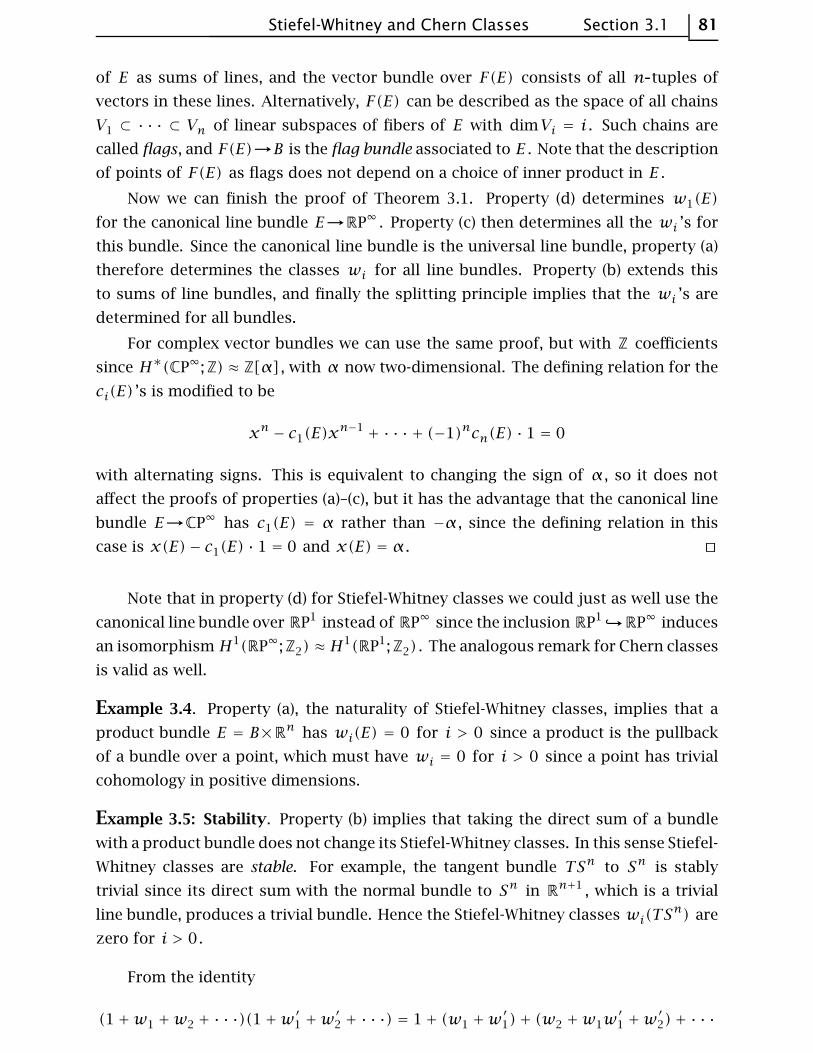
Stiefel-Whitney and Chern Classes Section 3.1 81
of E as sums of lines, and the vector bundle over F(E) consists of all n tuples of
vectors in these lines. Alternatively, F(E) can be described as the space of all chains
V1 ⊂ · · · ⊂ Vn of linear subspaces of fibers of E with dimVi = i . Such chains are
called flags, and F(E)→B is the flag bundle associated to E . Note that the description
of points of F(E) as flags does not depend on a choice of inner product in E .
Now we can finish the proof of Theorem 3.1. Property (d) determines w1(E)
for the canonical line bundle E→RP∞ . Property (c) then determines all the wi ’s for
this bundle. Since the canonical line bundle is the universal line bundle, property (a)
therefore determines the classes wi for all line bundles. Property (b) extends this
to sums of line bundles, and finally the splitting principle implies that the wi ’s are
determined for all bundles.
For complex vector bundles we can use the same proof, but with Z coefficients
since H∗(CP∞;Z) ≈ Z[α] , with α now two-dimensional. The defining relation for the
ci(E) ’s is modified to be
xn − c1(E)xn−1 + · · · + (−1)ncn(E) · 1 = 0
with alternating signs. This is equivalent to changing the sign of α , so it does not
affect the proofs of properties (a)–(c), but it has the advantage that the canonical line
bundle E→CP∞ has c1(E) = α rather than −α , since the defining relation in this
case is x(E)− c1(E) · 1 = 0 and x(E) = α . ⊔⊓
Note that in property (d) for Stiefel-Whitney classes we could just as well use the
canonical line bundle over RP1 instead of RP∞ since the inclusion RP1RP∞ induces
an isomorphism H1(RP∞;Z2) ≈ H1(RP1;Z2) . The analogous remark for Chern classes
is valid as well.
Example 3.4. Property (a), the naturality of Stiefel-Whitney classes, implies that a
product bundle E = B×Rn has wi(E) = 0 for i > 0 since a product is the pullback
of a bundle over a point, which must have wi = 0 for i > 0 since a point has trivial
cohomology in positive dimensions.
Example 3.5: Stability. Property (b) implies that taking the direct sum of a bundle
with a product bundle does not change its Stiefel-Whitney classes. In this sense Stiefel-
Whitney classes are stable. For example, the tangent bundle TSn to Sn is stably
trivial since its direct sum with the normal bundle to Sn in Rn+1 , which is a trivial
line bundle, produces a trivial bundle. Hence the Stiefel-Whitney classes wi(TSn) are
zero for i > 0.
From the identity
(1+w1 +w2 + · · ·)(1+w′1 +w
′2 + · · ·) = 1+ (w1 +w
′1)+ (w2 +w1w
′1 +w
′2)+ · · ·
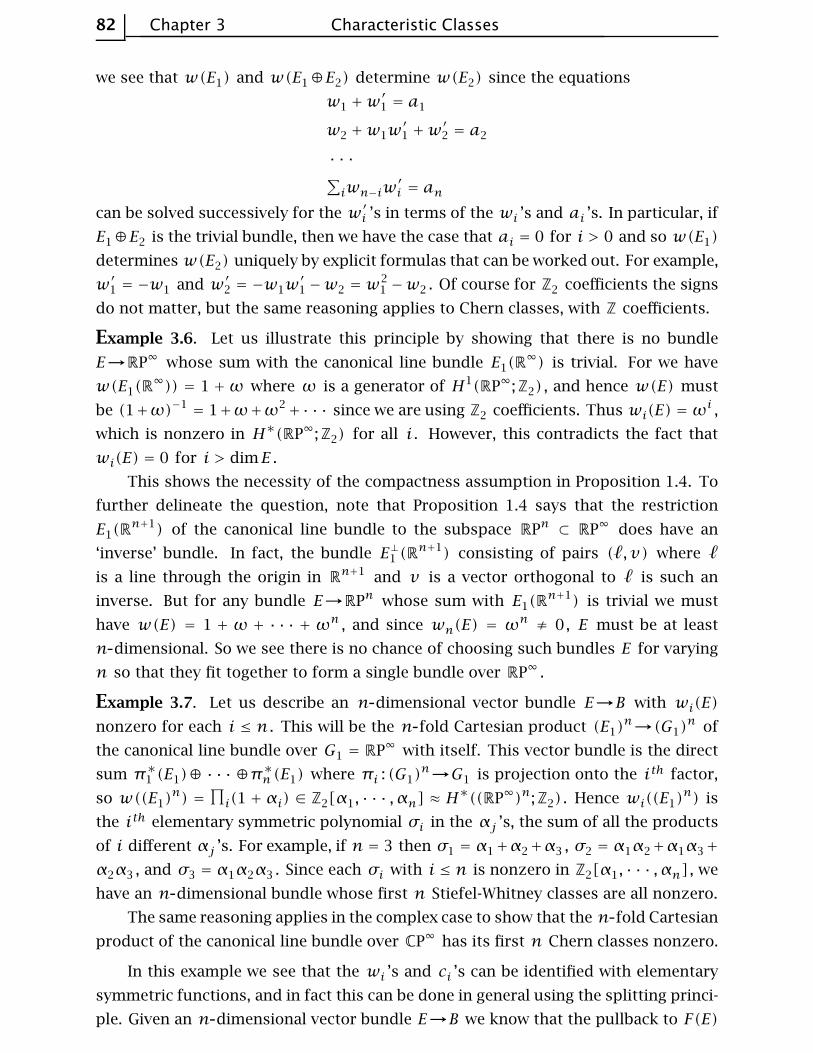
82 Chapter 3 Characteristic Classes
we see that w(E1) and w(E1⊕E2) determine w(E2) since the equations
w1 +w′1 = a1
w2 +w1w′1 +w
′2 = a2
· · ·∑iwn−iw
′i = an
can be solved successively for the w′i ’s in terms of the wi ’s and ai ’s. In particular, if
E1⊕E2 is the trivial bundle, then we have the case that ai = 0 for i > 0 and so w(E1)
determines w(E2) uniquely by explicit formulas that can be worked out. For example,
w′1 = −w1 and w′2 = −w1w′1−w2 = w
21 −w2 . Of course for Z2 coefficients the signs
do not matter, but the same reasoning applies to Chern classes, with Z coefficients.
Example 3.6. Let us illustrate this principle by showing that there is no bundle
E→RP∞ whose sum with the canonical line bundle E1(R∞) is trivial. For we have
w(E1(R∞)) = 1 +ω where ω is a generator of H1(RP∞;Z2) , and hence w(E) must
be (1+ω)−1 = 1+ω+ω2+· · · since we are using Z2 coefficients. Thus wi(E) =ωi ,
which is nonzero in H∗(RP∞;Z2) for all i . However, this contradicts the fact that
wi(E) = 0 for i > dimE .
This shows the necessity of the compactness assumption in Proposition 1.4. To
further delineate the question, note that Proposition 1.4 says that the restriction
E1(Rn+1) of the canonical line bundle to the subspace RPn ⊂ RP∞ does have an
‘inverse’ bundle. In fact, the bundle E⊥1 (Rn+1) consisting of pairs (ℓ, v) where ℓ
is a line through the origin in Rn+1 and v is a vector orthogonal to ℓ is such an
inverse. But for any bundle E→RPn whose sum with E1(Rn+1) is trivial we must
have w(E) = 1 + ω + · · · + ωn , and since wn(E) = ωn≠ 0, E must be at least
n dimensional. So we see there is no chance of choosing such bundles E for varying
n so that they fit together to form a single bundle over RP∞ .
Example 3.7. Let us describe an n dimensional vector bundle E→B with wi(E)
nonzero for each i ≤ n . This will be the n fold Cartesian product (E1)n→(G1)
n of
the canonical line bundle over G1 = RP∞ with itself. This vector bundle is the direct
sum π∗1 (E1)⊕ · · · ⊕π∗n (E1) where πi : (G1)
n→G1 is projection onto the ith factor,
so w((E1)n) =
∏i(1 + αi) ∈ Z2[α1, · · · , αn] ≈ H
∗((RP∞)n;Z2) . Hence wi((E1)n) is
the ith elementary symmetric polynomial σi in the αj ’s, the sum of all the products
of i different αj ’s. For example, if n = 3 then σ1 = α1+α2+α3 , σ2 = α1α2+α1α3+
α2α3 , and σ3 = α1α2α3 . Since each σi with i ≤ n is nonzero in Z2[α1, · · · , αn] , we
have an n dimensional bundle whose first n Stiefel-Whitney classes are all nonzero.
The same reasoning applies in the complex case to show that the n fold Cartesian
product of the canonical line bundle over CP∞ has its first n Chern classes nonzero.
In this example we see that the wi ’s and ci ’s can be identified with elementary
symmetric functions, and in fact this can be done in general using the splitting princi-
ple. Given an n dimensional vector bundle E→B we know that the pullback to F(E)
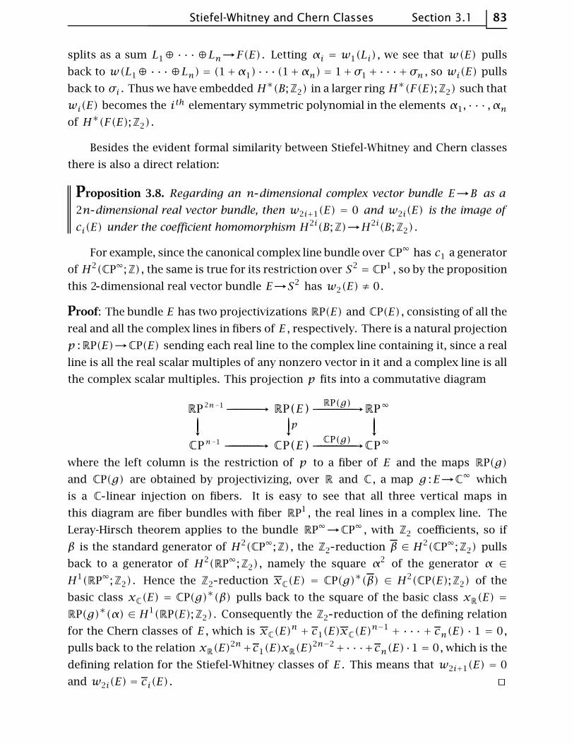
Stiefel-Whitney and Chern Classes Section 3.1 83
splits as a sum L1⊕ · · · ⊕Ln→F(E) . Letting αi = w1(Li) , we see that w(E) pulls
back to w(L1⊕ · · · ⊕Ln) = (1+α1) · · · (1+αn) = 1+σ1+· · ·+σn , so wi(E) pulls
back to σi . Thus we have embedded H∗(B;Z2) in a larger ring H∗(F(E);Z2) such that
wi(E) becomes the ith elementary symmetric polynomial in the elements α1, · · · , αnof H∗(F(E);Z2) .
Besides the evident formal similarity between Stiefel-Whitney and Chern classes
there is also a direct relation:
Proposition 3.8. Regarding an n dimensional complex vector bundle E→B as a
2n dimensional real vector bundle, then w2i+1(E) = 0 and w2i(E) is the image of
ci(E) under the coefficient homomorphism H2i(B;Z)→H2i(B;Z2) .
For example, since the canonical complex line bundle over CP∞ has c1 a generator
of H2(CP∞;Z) , the same is true for its restriction over S2 = CP1 , so by the proposition
this 2 dimensional real vector bundle E→S2 has w2(E) ≠ 0.
Proof: The bundle E has two projectivizations RP(E) and CP(E) , consisting of all the
real and all the complex lines in fibers of E , respectively. There is a natural projection
p :RP(E)→CP(E) sending each real line to the complex line containing it, since a real
line is all the real scalar multiples of any nonzero vector in it and a complex line is all
the complex scalar multiples. This projection p fits into a commutative diagram
where the left column is the restriction of p to a fiber of E and the maps RP(g)
and CP(g) are obtained by projectivizing, over R and C , a map g :E→C∞ which
is a C linear injection on fibers. It is easy to see that all three vertical maps in
this diagram are fiber bundles with fiber RP1 , the real lines in a complex line. The
Leray-Hirsch theorem applies to the bundle RP∞→CP∞ , with Z2 coefficients, so if
β is the standard generator of H2(CP∞;Z) , the Z2 reduction β ∈ H2(CP∞;Z2) pulls
back to a generator of H2(RP∞;Z2) , namely the square α2 of the generator α ∈
H1(RP∞;Z2) . Hence the Z2 reduction xC(E) = CP(g)∗(β) ∈ H2(CP(E);Z2) of the
basic class xC(E) = CP(g)∗(β) pulls back to the square of the basic class xR(E) =
RP(g)∗(α) ∈ H1(RP(E);Z2) . Consequently the Z2 reduction of the defining relation
for the Chern classes of E , which is xC(E)n + c1(E)xC(E)
n−1 + · · · + cn(E) · 1 = 0,
pulls back to the relation xR(E)2n+c1(E)xR(E)
2n−2+· · ·+cn(E)·1 = 0, which is the
defining relation for the Stiefel-Whitney classes of E . This means that w2i+1(E) = 0
and w2i(E) = ci(E) . ⊔⊓
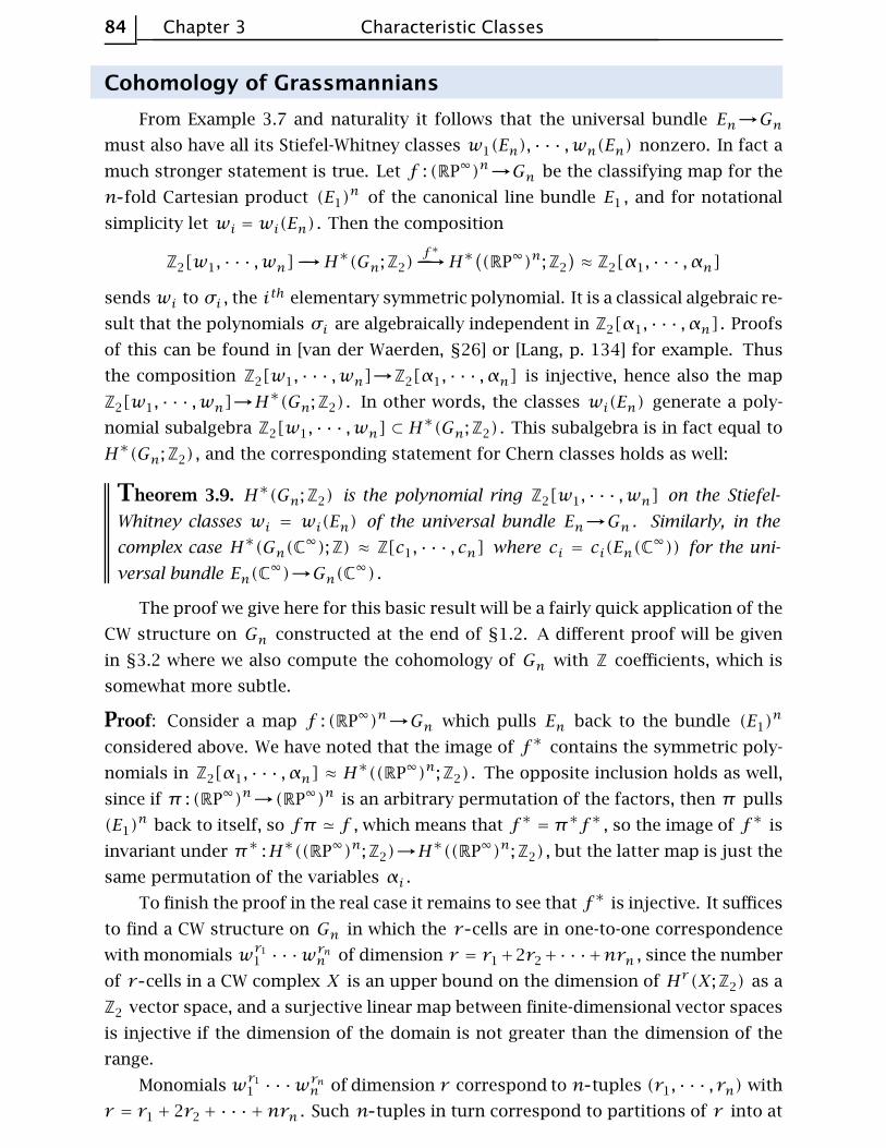
84 Chapter 3 Characteristic Classes
Cohomology of Grassmannians
From Example 3.7 and naturality it follows that the universal bundle En→Gnmust also have all its Stiefel-Whitney classes w1(En), · · · ,wn(En) nonzero. In fact a
much stronger statement is true. Let f : (RP∞)n→Gn be the classifying map for the
n fold Cartesian product (E1)n of the canonical line bundle E1 , and for notational
simplicity let wi = wi(En) . Then the composition
Z2[w1, · · · ,wn] -→H∗(Gn;Z2)f∗
-----→H∗((RP∞)n;Z2
)≈ Z2[α1, · · · , αn]
sends wi to σi , the ith elementary symmetric polynomial. It is a classical algebraic re-
sult that the polynomials σi are algebraically independent in Z2[α1, · · · , αn] . Proofs
of this can be found in [van der Waerden, §26] or [Lang, p. 134] for example. Thus
the composition Z2[w1, · · · ,wn]→Z2[α1, · · · , αn] is injective, hence also the map
Z2[w1, · · · ,wn]→H∗(Gn;Z2) . In other words, the classes wi(En) generate a poly-
nomial subalgebra Z2[w1, · · · ,wn] ⊂ H∗(Gn;Z2) . This subalgebra is in fact equal to
H∗(Gn;Z2) , and the corresponding statement for Chern classes holds as well:
Theorem 3.9. H∗(Gn;Z2) is the polynomial ring Z2[w1, · · · ,wn] on the Stiefel-
Whitney classes wi = wi(En) of the universal bundle En→Gn . Similarly, in the
complex case H∗(Gn(C∞);Z) ≈ Z[c1, · · · , cn] where ci = ci(En(C
∞)) for the uni-
versal bundle En(C∞)→Gn(C∞) .
The proof we give here for this basic result will be a fairly quick application of the
CW structure on Gn constructed at the end of §1.2. A different proof will be given
in §3.2 where we also compute the cohomology of Gn with Z coefficients, which is
somewhat more subtle.
Proof: Consider a map f : (RP∞)n→Gn which pulls En back to the bundle (E1)n
considered above. We have noted that the image of f∗ contains the symmetric poly-
nomials in Z2[α1, · · · , αn] ≈ H∗((RP∞)n;Z2) . The opposite inclusion holds as well,
since if π : (RP∞)n→(RP∞)n is an arbitrary permutation of the factors, then π pulls
(E1)n back to itself, so fπ ≃ f , which means that f∗ = π∗f∗ , so the image of f∗ is
invariant under π∗ :H∗((RP∞)n;Z2)→H∗((RP∞)n;Z2) , but the latter map is just the
same permutation of the variables αi .
To finish the proof in the real case it remains to see that f∗ is injective. It suffices
to find a CW structure on Gn in which the r cells are in one-to-one correspondence
with monomials wr1
1 · · ·wrnn of dimension r = r1+2r2+· · ·+nrn , since the number
of r cells in a CW complex X is an upper bound on the dimension of Hr (X;Z2) as a
Z2 vector space, and a surjective linear map between finite-dimensional vector spaces
is injective if the dimension of the domain is not greater than the dimension of the
range.
Monomials wr1
1 · · ·wrnn of dimension r correspond to n tuples (r1, · · · , rn) with
r = r1 + 2r2+ · · ·+nrn . Such n tuples in turn correspond to partitions of r into at
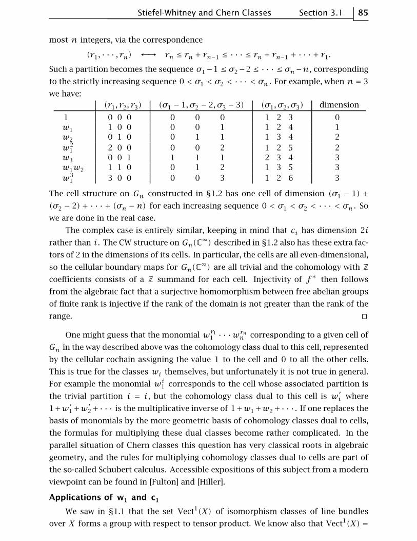
Stiefel-Whitney and Chern Classes Section 3.1 85
most n integers, via the correspondence
(r1, · · · , rn) ←→ rn ≤ rn + rn−1 ≤ · · · ≤ rn + rn−1 + · · · + r1.
Such a partition becomes the sequence σ1−1 ≤ σ2−2 ≤ · · · ≤ σn−n , corresponding
to the strictly increasing sequence 0 < σ1 < σ2 < · · · < σn . For example, when n = 3
we have:
(r1, r2, r3) (σ1 − 1, σ2 − 2, σ3 − 3) (σ1, σ2, σ3) dimension
1 0 0 0 0 0 0 1 2 3 0
w1 1 0 0 0 0 1 1 2 4 1
w2 0 1 0 0 1 1 1 3 4 2
w21 2 0 0 0 0 2 1 2 5 2
w3 0 0 1 1 1 1 2 3 4 3
w1w2 1 1 0 0 1 2 1 3 5 3
w31 3 0 0 0 0 3 1 2 6 3
The cell structure on Gn constructed in §1.2 has one cell of dimension (σ1 − 1) +
(σ2 − 2)+ · · · + (σn −n) for each increasing sequence 0 < σ1 < σ2 < · · · < σn . So
we are done in the real case.
The complex case is entirely similar, keeping in mind that ci has dimension 2i
rather than i . The CW structure on Gn(C∞) described in §1.2 also has these extra fac-
tors of 2 in the dimensions of its cells. In particular, the cells are all even-dimensional,
so the cellular boundary maps for Gn(C∞) are all trivial and the cohomology with Z
coefficients consists of a Z summand for each cell. Injectivity of f∗ then follows
from the algebraic fact that a surjective homomorphism between free abelian groups
of finite rank is injective if the rank of the domain is not greater than the rank of the
range. ⊔⊓
One might guess that the monomial wr1
1 · · ·wrnn corresponding to a given cell of
Gn in the way described above was the cohomology class dual to this cell, represented
by the cellular cochain assigning the value 1 to the cell and 0 to all the other cells.
This is true for the classes wi themselves, but unfortunately it is not true in general.
For example the monomial wi1 corresponds to the cell whose associated partition is
the trivial partition i = i , but the cohomology class dual to this cell is w′i where
1+w′1+w′2+· · · is the multiplicative inverse of 1+w1+w2+· · · . If one replaces the
basis of monomials by the more geometric basis of cohomology classes dual to cells,
the formulas for multiplying these dual classes become rather complicated. In the
parallel situation of Chern classes this question has very classical roots in algebraic
geometry, and the rules for multiplying cohomology classes dual to cells are part of
the so-called Schubert calculus. Accessible expositions of this subject from a modern
viewpoint can be found in [Fulton] and [Hiller].
Applications of w1 and c1
We saw in §1.1 that the set Vect1(X) of isomorphism classes of line bundles
over X forms a group with respect to tensor product. We know also that Vect1(X) =
86 Chapter 3 Characteristic Classes
[X,G1(R∞)] , and G1(R
∞) is just RP∞ , an Eilenberg-MacLane space K(Z2,1) . It is a
basic fact in algebraic topology that [X,K(G,n)] ≈ Hn(X;G) when X has the homo-
topy type of a CW complex; see Theorem 4.56 of [AT], for example. Thus one might
ask whether the groups Vect1(X) and H1(X;Z2) are isomorphic. For complex line
bundles we have G1(C∞) = CP∞ , and this is a K(Z,2) , so the corresponding question
is whether Vect1C(X) is isomorphic to H2(X;Z) .
Proposition 3.10. The function w1 : Vect1(X)→H1(X;Z2) is a homomorphism, and
is an isomorphism if X has the homotopy type of a CW complex. The same is also
true for c1 : Vect1C(X)→H2(X;Z) .
Proof: The argument is the same in both the real and complex cases, so for def-
initeness let us describe the complex case. To show that c1 : Vect1C(X)→H2(X) is
a homomorphism, we first prove that c1(L1⊗L2) = c1(L1) + c1(L2) for the bundle
L1⊗L2→G1×G1 where L1 and L2 are the pullbacks of the canonical line bundle
L→G1 = CP∞ under the projections p1, p2 :G1×G1→G1 onto the two factors. Since
c1(L) is the generator α of H2(CP∞) , we know that H∗(G1×G1) ≈ Z[α1, α2] where
αi = p∗i (α) = c1(Li) . The inclusion G1∨G1 ⊂ G1×G1 induces an isomorphism on H2 ,
so to compute c1(L1⊗L2) it suffices to restrict to G1∨G1 . Over the first G1 the bundle
L2 is the trivial line bundle, so the restriction of L1⊗L2 over this G1 is L1⊗1 ≈ L1 .
Similarly, L1⊗L2 restricts to L2 over the second G1 . So c1(L1⊗L2) restricted to
G1∨G1 is α1+α2 restricted to G1∨G1 . Hence c1(L1⊗L2) = α1+α2 = c1(L1)+c1(L2) .
The general case of the formula c1(E1⊗E2) = c1(E1)+ c1(E2) for line bundles E1
and E2 now follows by naturality: We have E1 ≈ f∗1 (L) and E2 ≈ f
∗2 (L) for maps
f1, f2 :X→G1 . For the map F = (f1, f2) :X→G1×G1 we have F∗(Li) = f∗i (L) ≈ Ei ,
so
c1(E1⊗E2) = c1(F∗(L1)⊗F
∗(L2)) = c1(F∗(L1⊗L2)) = F
∗(c1(L1⊗L2))
= F∗(c1(L1)+ c1(L2)) = F∗(c1(L1))+ F
∗(c1(L2))
= c1(F∗(L1))+ c1(F
∗(L2)) = c1(E1)+ c1(E2).
As noted above, if X is a CW complex, there is a bijection [X,CP∞] ≈ H2(X;Z) ,
and the more precise statement is that this bijection is given by the map [f ]֏f∗(u)
for some class u ∈ H2(CP∞;Z) . The class u must be a generator, otherwise the map
would not always be surjective. Which of the two generators we choose for u is
not important, so we may take it to be the class α . The map [f ]֏ f∗(α) factors
as the composition [X,CP∞]→Vect1C(X)→H2(X;Z) , [f ]֏ f∗(L)֏ c1(f
∗(L)) =
f∗(c1(L)) = f∗(α) . The first map in this composition is a bijection, so since the
composition is a bijection, the second map c1 must be a bijection also. ⊔⊓
The first Stiefel-Whitney class w1 is closely related to orientability:
Stiefel-Whitney and Chern Classes Section 3.1 87
Proposition 3.11. A vector bundle E→X is orientable iff w1(E) = 0 , assuming that
X is homotopy equivalent to a CW complex.
Thus w1 can be viewed as the obstruction to orientability of vector bundles. An
interpretation of the other classes wi as obstructions will be given in the Appendix
to this chapter.
Proof: Without loss we may assume X is a CW complex. By restricting to path-
components we may further assume X is connected. There are natural isomorphisms
(∗) H1(X;Z2)≈------------→Hom(H1(X),Z2)
≈------------→Hom(π1(X),Z2)
from the universal coefficient theorem and the fact that H1(X) is the abelianization of
π1(X) . When X = Gn we have π1(Gn) ≈ Z2 , and w1(En) ∈ H1(Gn;Z2) corresponds
via (∗) to this isomorphism π1(Gn) ≈ Z2 since w1(En) is the unique nontrivial el-
ement of H1(Gn;Z2) . By naturality of (∗) it follows that for any map f :X→Gn ,
f∗(w1(En)) corresponds under (∗) to the homomorphism f∗ :π1(X)→π1(Gn) ≈
Z2 . Thus if we choose f so that f∗(En) is a given vector bundle E , we have w1(E)
corresponding under (∗) to the induced map f∗ :π1(X)→π1(Gn) ≈ Z2 . Hence
w1(E) = 0 iff this f∗ is trivial, which is exactly the condition for lifting f to the
universal cover Gn , i.e., orientability of E . ⊔⊓
88 Chapter 3 Characteristic Classes
3.2. Euler and Pontryagin Classes
A characteristic class can be defined to be a function associating to each vector
bundle E→B of dimension n a class x(E) ∈ Hk(B;G) , for some fixed n and k , such
that the naturality property x(f∗(E)) = f∗(x(E)) is satisfied. In particular, for the
universal bundle En→Gn there is the class x = x(En) ∈ Hk(Gn;G) . Conversely, any
element x ∈ Hk(Gn;G) defines a characteristic class by the rule x(E) = f∗(x) where
E ≈ f∗(En) for f :B→Gn . Since f is unique up to homotopy, x(E) is well-defined,
and it is clear that the naturality property is satisfied. Thus characteristic classes
correspond bijectively with cohomology classes of Gn .
With Z2 coefficients all characteristic classes are simply polynomials in the Stiefel-
Whitney classes since we showed in Theorem 3.9 that H∗(Gn;Z2) is the polyno-
mial ring Z2[w1, · · · ,wn] . Similarly for complex vector bundles all characteristic
classes with Z coefficients are polynomials in the Chern classes since H∗(Gn(C);Z) ≈
Z[c1, · · · , cn] . Our goal in this section is to describe the more refined characteris-
tic classes for real vector bundles that arise when we take cohomology with integer
coefficients rather than Z2 coefficients.
The main tool we will use will be the Gysin exact sequence associated to an
n dimensional real vector bundle p :E→B . This is an easy consequence of the Thom
isomorphism Φ :Hi(B)→Hi+n(D(E), S(E)) defined by Φ(b) = p∗(b)` c for a Thom
class c ∈ Hn(D(E), S(E)) , a class whose restriction to each fiber is a generator of
Hn(Dn, Sn−1) . The map Φ is an isomorphism whenever a Thom class exists, as shown
in Corollary 4D.9 of [AT]. Thom classes with Z coefficients exist for all orientable real
vector bundles, and with Z2 coefficients they exist for all vector bundles. This is
shown in Theorem 4D.10 of [AT].
Once one has the Thom isomorphism, this gives the Gysin sequence as the lower
row of the following commutative diagram, whose upper row is the exact sequence
for the pair (D(E), S(E)) :
The vertical map p∗ is an isomorphism since p is a homotopy equivalence from
D(E) to B . The Euler class e ∈ Hn(B) is defined to be (p∗)−1j∗(c) , or in other words
the restriction of the Thom class to the zero section of E . The square containing
the map `e commutes since for b ∈ Hi−n(B) we have j∗Φ(b) = j∗(p∗(b) ` c) =p∗(b) ` j∗(c) , which equals p∗(b ` e) = p∗(b) ` p∗(e) since p∗(e) = j∗(c) . The
Euler class can also be defined as the class corresponding to c ` c under the Thom
isomorphism, since Φ(e) = p∗(e)` c = j∗(c)` c = c ` c .
As a warm-up application of the Gysin sequence let us use it to give a different
proof of Theorem 3.9 computing H∗(Gn;Z2) and H∗(Gn(C);Z) . Consider first the
Euler and Pontryagin Classes Section 3.2 89
real case. The proof will be by induction on n using the Gysin sequence for the univer-
sal bundle Enπ-----→Gn . The sphere bundle S(En) is the space of pairs (v, ℓ) where ℓ
is an n dimensional linear subspace of R∞ and v is a unit vector in ℓ . There is a nat-
ural map p :S(En)→Gn−1 sending (v, ℓ) to the (n−1) dimensional linear subspace
v⊥ ⊂ ℓ orthogonal to v . It is an exercise to check that p is a fiber bundle. Its fiber is
S∞ , all the unit vectors in R∞ orthogonal to a given (n − 1) dimensional subspace.
Since S∞ is contractible, p induces an isomorphism on all homotopy groups, hence
also on all cohomology groups. Using this isomorphism p∗ the Gysin sequence, with
Z2 coefficients, has the form
· · · -→Hi(Gn)`e------------→Hi+n(Gn)
η-----→Hi+n(Gn−1) -→Hi+1(Gn) -→· · ·
where e ∈ Hn(Gn;Z2) is the Z2 Euler class.
We show first that η(wj(En)) = wj(En−1) . By definition the map η is the com-
position H∗(Gn)→H∗(S(En))≈←------ H∗(Gn−1) induced from Gn−1
p←------ S(En)
π-----→Gn .
The pullback π∗(En) consists of triples (v,w, ℓ) where ℓ ∈ Gn and v,w ∈ ℓ with
v a unit vector. This pullback splits naturally as a sum L⊕p∗(En−1) where L is the
subbundle of triples (v, tv, ℓ) , t ∈ R , and p∗(En−1) consists of the triples (v,w, ℓ)
with w ∈ v⊥ . The line bundle L is trivial, having the section (v,v, ℓ) . Thus the coho-
mology homomorphism π∗ takes wj(En)) to wj(L⊕p∗(En−1)) = wj(p
∗(En−1)) =
p∗(wj(En−1)) , so η(wj(En)) =wj(En−1) .
By induction on n , H∗(Gn−1) is the polynomial ring on the classes wj(En−1) ,
j < n . The induction can start with the case n = 1, where G1 = RP∞ and H∗(RP∞) ≈
Z2[w1] since w1(E1) is a generator of H1(RP∞;Z2) . Or we could start with the trivial
case n = 0. Since η(wj(En)) = wj(En−1) , the maps η are surjective and the Gysin
sequence splits into short exact sequences
0 -→Hi(Gn)`e------------→Hi+n(Gn)
η-----→Hi+n(Gn−1) -→0
The image of `e :H0(Gn)→Hn(Gn) is a Z2 generated by e . By exactness, this Z2
is the kernel of η :Hn(Gn)→Hn(Gn−1) . The class wn(En) lies in this kernel since
wn(En−1) = 0. Moreover, wn(En) ≠ 0, since if wn(En) = 0 then wn is zero for all
n dimensional vector bundles, but the bundle E→RP∞ which is the direct sum of n
copies of the canonical line bundle has total Stiefel-Whitney class w(E) = (1 + α)n ,
where α generates H1(RP∞) , hence wn(E) = αn≠ 0. Thus e and wn(En) generate
the same Z2 , so e =wn(En) .
Now we argue that each element ξ ∈ Hk(Gn) can be expressed as a unique poly-
nomial in the classes wi = wi(En) , by induction on k . First, η(ξ) is a unique polyno-
mial f in the wi(En−1) ’s by the basic induction on n . Then ξ−f(w1, · · · ,wn−1) is in
Kerη = Im(`wn) , hence has the form ζ`wn for ζ ∈ Hk−n(Gn) which is unique since
`wn is injective. By induction on k , ζ is a unique polynomial g in the wi ’s. Thus
we have ξ expressed uniquely as a polynomial f(w1, · · · ,wn−1)+wng(w1, · · · ,wn) .
90 Chapter 3 Characteristic Classes
Since every polynomial in w1, · · · ,wn has a unique expression in this form, the the-
orem follows in the real case.
Virtually the same argument works in the complex case. We noted earlier that
complex vector bundles always have a Gysin sequence with Z coefficients. The only
elaboration needed to extend the preceding proof to the complex case is at the step
where we showed the Z2 Euler class is wn . The argument from the real case shows
that cn is a multiple me for some m ∈ Z , e being now the Z Euler class. Then
for the bundle E→CP∞ which is the direct sum of n copies of the canonical line
bundle, classified by f :CP∞→Gn(C∞) , we have αn = cn(E) = f∗(cn) =mf
∗(e) in
H2n(CP∞;Z) ≈ Z , with αn a generator, hence m = ±1 and e = ±cn . The rest of the
proof goes through without change.
We can also compute H∗(Gn;Z2) where Gn is the oriented Grassmannian. To
state the result, let π : Gn→Gn be the covering projection, so En = π∗(En) , and let
wi = wi(En) = π∗(wi) ∈ H
i(Gn;Z2) , where wi = wi(En) .
Proposition 3.12. π∗ :H∗(Gn;Z2)→H∗(Gn;Z2) is surjective with kernel the ideal
generated by w1 , hence H∗(Gn;Z2) ≈ Z2[w2, · · · , wn] .
This is just the answer one would hope for. Since Gn is simply-connected, w1 has
to be zero, so the isomorphism H∗(Gn;Z2) ≈ Z2[w2, · · · , wn] is the simplest thing
that could happen.
Proof: The 2 sheeted covering π : Gn→Gn can be regarded as the unit sphere bundle
of a 1 dimensional vector bundle, so we have a Gysin sequence beginning
0 -→H0(Gn;Z2) -→H0(Gn;Z2) -→H0(Gn;Z2)`x------------→H1(Gn;Z2)
where x ∈ H1(Gn;Z2) is the Z2 Euler class. Since Gn is connected, H0(Gn;Z2) ≈
Z2 and so the map `x is injective, hence x = w1 , the only nonzero element of
H1(Gn;Z2) . Since H∗(Gn;Z2) ≈ Z2[w1, · · · ,wn] , the map `w1 is injective in all
dimensions, so the Gysin sequence breaks up into short exact sequences
0 -→Hi−1(Gn;Z2)`w1-----------------------→Hi(Gn;Z2)
π∗------------→Hi(Gn;Z2) -→0
from which the conclusion is immediate. ⊔⊓
The goal for the rest of this section is to determine H∗(Gn;Z) and H∗(Gn;Z) ,
or in other words, to find all characteristic classes for real vector bundles with Z
coefficients, rather than the Z2 coefficients used for Stiefel-Whitney classes. It turns
out that H∗(Gn;Z) , modulo elements of order 2 which are just certain polynomials
in Stiefel-Whitney classes, is a polynomial ring Z[p1, p2, · · ·] on certain classes pi of
dimension 4i , called Pontryagin classes. There is a similar statement for H∗(Gn;Z) ,
but with one of the Pontryagin classes replaced by an Euler class when n is even.
Euler and Pontryagin Classes Section 3.2 91
The Euler Class
Recall that the Euler class e(E) ∈ Hn(B;Z) of an orientable n dimensional vector
bundle E→B is the restriction of a Thom class c ∈ Hn(D(E), S(E);Z) to the zero
section, that is, the image of c under the composition
Hn(D(E), S(E);Z)→Hn(D(E);Z)→Hn(B;Z)
where the first map is the usual passage from relative to absolute cohomology and the
second map is induced by the inclusion BD(E) as the zero section. By its definition,
e(E) depends on the choice of c . However, the assertion (*) in the construction of a
Thom class in Theorem 4D.10 of [AT] implies that c is determined by its restriction to
each fiber, and the restriction of c to each fiber is in turn determined by an orientation
of the bundle, so in fact e(E) depends only on the choice of an orientation of E .
Choosing the opposite orientation changes the sign of c . There are exactly two choices
of orientation for each path-component of B .
Here are the basic properties of Euler classes e(E) ∈ Hn(B;Z) associated to ori-
ented n dimensional vector bundles E→B :
Proposition 3.13.
(a) An orientation of a vector bundle E→B induces an orientation of a pullback
bundle f∗(E) such that e(f∗(E)) = f∗(e(E)) .
(b) Orientations of vector bundles E1→B and E2→B determine an orientation of
the sum E1⊕E2 such that e(E1⊕E2) = e(E1)` e(E2) .
(c) For an orientable n dimensional real vector bundle E , the coefficient homomor-
phism Hn(B;Z)→Hn(B;Z2) carries e(E) to wn(E) . For an n dimensional com-
plex vector bundle E there is the relation e(E) = cn(E) ∈ H2n(B;Z) , for a suitable
choice of orientation of E .
(d) e(E) = −e(E) if the fibers of E have odd dimension.
(e) e(E) = 0 if E has a nowhere-zero section.
Proof: (a) For an n dimensional vector bundle E , let E′ ⊂ E be the complement of
the zero section. A Thom class for E can be viewed as an element of Hn(E, E′;Z)
which restricts to a generator of Hn(Rn,Rn−{0};Z) in each fiber Rn . For a pullback
f∗(E) , we have a map f :f∗(E)→E which is a linear isomorphism in each fiber, so
f∗(c(E)) restricts to a generator of Hn(Rn,Rn − {0};Z) in each fiber Rn of f∗(E) .
Thus f∗(c(E)) = c(f∗(E)) . Passing from relative to absolute cohomology classes
and then restricting to zero sections, we get e(f∗(E)) = f∗(e(E)) .
(b) There is a natural projection p1 :E1⊕E2→E1 which is linear in each fiber, and
likewise we have p2 :E1⊕E2→E2 . If E1 is m dimensional we can view a Thom class
c(E1) as lying in Hm(E1, E′1) where E′1 is the complement of the zero section in E1 .
Similarly we have a Thom class c(E2) ∈ Hn(E2, E
′2) if E2 has dimension n . Then
the product p∗1 (c(E1)) ` p∗2 (c(E2)) is a Thom class for E1⊕E2 since in each fiber
92 Chapter 3 Characteristic Classes
Rm×Rn = Rm+n we have the cup product
Hm(Rm+n,Rm+n −Rn)×Hn(Rm+n,Rm+n −Rm)→Hm+n(Rm+n,Rm+n − {0})
which takes generator cross generator to generator by the calculations in Example 3.11
of [AT]. Passing from relative to absolute cohomology and restricting to the zero sec-
tion, we get the relation e(E1⊕E2) = e(E1)` e(E2) .
(c) We showed this for the universal bundle in the calculation of the cohomology of
Grassmannians a couple pages back, so by the naturality property in (a) it holds for
all bundles.
(d) When we defined the Euler class we observed that it could also be described as the
element of Hn(B;Z) corresponding to c ` c ∈ H2n(D(E), S(E),Z) under the Thom
isomorphism. If n is odd, the basic commutativity relation for cup products gives
c ` c = −c ` c , so e(E) = −e(E) .
(e) A nowhere-zero section of E gives rise to a section s :B→S(E) by normalizing
vectors to have unit length. Then in the exact sequence
Hn(D(E), S(E);Z)j∗
-----→Hn(D(E);Z)i∗-----→Hn(S(E);Z)
the map i∗ is injective since the composition D(E) -→Bs-----→S(E)
i-----→D(E) is homo-
topic to the identity. Since i∗ is injective, the map j∗ is zero by exactness, and hence
e(E) = 0 from the definition of the Euler class. ⊔⊓
Consider the tangent bundle TSn to Sn . This bundle is orientable since its base
Sn is simply-connected if n > 1, while if n = 1, TS1 is just the product S1×R . When
n is odd, e(TSn) = 0 either by part (d) of the proposition since H∗(Sn;Z) has no
elements of order two, or by part (e) since there is a nonzero tangent vector field to
Sn when n is odd, namely s(x1, · · · , xn+1) = (−x2, x1, · · · ,−xn+1, xn) . However,
when n is even e(TSn) is nonzero:
Proposition 3.14. For even n , e(TSn) is twice a generator of Hn(Sn;Z) .
Proof: Let E′ ⊂ E = TSn be the complement of the zero section. Under the Thom
isomorphism the Euler class e(TSn) corresponds to the square of a Thom class
c ∈ Hn(E, E′) , so it suffices to show that c2 is twice a generator of H2n(E, E′) . Let
A ⊂ Sn×Sn consist of the antipodal pairs (x,−x) . De-
fine a homeomorphism f :Sn×Sn − A→E sending a pair
(x,y) ∈ Sn×Sn − A to the vector from x to the point of
intersection of the line through −x and y with the tangent
plane at x . The diagonal D = {(x,x)} corresponds under
f to the zero section of E . Excision then gives the first of
the following isomorphisms:
H∗(E, E′) ≈ H∗(Sn×Sn, Sn×Sn −D) ≈ H∗(Sn×Sn, A) ≈ H∗(Sn×Sn,D),
Euler and Pontryagin Classes Section 3.2 93
The second isomorphism holds since Sn×Sn − D deformation retracts onto A by
sliding a point y ≠ ±x along the great circle through x and y to −x , and the third
comes from the homeomorphism (x,y)֏ (x,−y) of Sn×Sn interchanging D and
A . From the long exact sequence of the pair (Sn×Sn,D) we extract a short exact
sequence
0→Hn(Sn×Sn,D)→Hn(Sn×Sn)→Hn(D)→0
The middle group Hn(Sn×Sn) has generators α , β which are pullbacks of a gener-
ator of Hn(Sn) under the two projections Sn×Sn→Sn . Both α and β restrict to
the same generator of Hn(D) since the two projections Sn×Sn→Sn restrict to the
same homeomorphism D ≈ Sn , so α−β generates Hn(Sn×Sn,D) , the kernel of the
restriction map Hn(Sn×Sn)→Hn(D) . Thus α − β corresponds to the Thom class
and (α−β)2 = −αβ−βα , which equals −2αβ if n is even. This is twice a generator
of H2n(Sn×Sn,D) ≈ H2n(Sn×Sn) . ⊔⊓
It is a fairly elementary theorem in differential topology that the Euler class of
the unit tangent bundle of a closed, connected, orientable smooth manifold Mn is
|χ(M)| times a generator of Hn(M) , where χ(M) is the Euler characteristic of M ;
see for example [Milnor-Stasheff]. This agrees with what we have just seen in the case
M = Sn , and is the reason for the name ‘Euler class.’
One might ask which elements of Hn(Sn) can occur as Euler classes of vector
bundles E→Sn in the nontrivial case that n is even. If we form the pullback of the
tangent bundle TSn by a map Sn→Sn of degree d , we realize 2d times a generator,
by part (a) of the preceding proposition, so all even multiples of a generator of Hn(Sn)
are realizable. To investigate odd multiples, consider the Thom space T(E) . This
has integral cohomology consisting of Z ’s in dimensions 0, n , and 2n by the Thom
isomorphism, which also says that the Thom class c is a generator of Hn(T(E)) . We
know that the Euler class corresponds under the Thom isomorphism to c`c , so e(E)
is k times a generator of Hn(Sn) iff c` c is k times a generator of H2n(T(E)) . This
is precisely the context of the Hopf invariant, and the solution of the Hopf invariant
one problem in Chapter 2 shows that c ` c can be an odd multiple of a generator
only if n = 2, 4, or 8. In these three cases there is a bundle E→Sn for which c ` c
is a generator of H2n(T(E)) , namely the vector bundle whose unit sphere bundle is
the complex, quaternionic, or octonionic Hopf bundle, and whose Thom space, the
mapping cone of the sphere bundle, is the associated projective plane CP2 , HP2 , or
OP2 . Since we can realize a generator of Hn(Sn) as an Euler class in these three cases,
we can realize any multiple of a generator by taking pullbacks as before.
94 Chapter 3 Characteristic Classes
Pontryagin Classes
The easiest definition of the Pontryagin classes pi(E) ∈ H4i(B;Z) associated to
a real vector bundle E→B is in terms of Chern classes. For a real vector bundle
E→B , its complexification is the complex vector bundle EC→B obtained from the
real vector bundle E⊕E by defining scalar multiplication by the complex number i
in each fiber Rn⊕Rn via the familiar rule i(x,y) = (−y,x) . Thus each fiber Rn
of E becomes a fiber Cn of EC . The Pontryagin class pi(E) is then defined to be
(−1)ic2i(EC) ∈ H4i(B;Z) . The sign (−1)i is introduced in order to avoid a sign in the
formula in (b) of the next proposition. The reason for restricting attention to the even
Chern classes c2i(EC) is that the odd classes c2i+1(E
C) turn out to be expressible in
terms of Stiefel-Whitney classes, and hence give nothing new. The exercises at the
end of the section give an explicit formula.
Here is how Pontryagin classes are related to Stiefel-Whitney and Euler classes:
Proposition 3.15.
(a) For a real vector bundle E→B , pi(E) maps to w2i(E)2 under the coefficient
homomorphism H4i(B;Z)→H4i(B;Z2) .
(b) For an orientable real 2n dimensional vector bundle with Euler class e(E) ∈
H2n(B;Z) , pn(E) = e(E)2 .
Note that statement (b) is independent of the choice of orientation of E since the
Euler class is squared.
Proof: (a) By Proposition 3.8, c2i(EC) reduces mod 2 to w4i(E⊕E) , which equals
w2i(E)2 since w(E⊕E) = w(E)2 and squaring is an additive homomorphism mod 2.
(b) First we need to determine the relationship between the two orientations of EC ≈
E⊕E , one coming from the canonical orientation of the complex bundle EC , the
other coming from the orientation of E⊕E determined by an orientation of E . If
v1, · · · , v2n is a basis for a fiber of E agreeing with the given orientation, then EC
is oriented by the ordered basis v1, iv1, · · · , v2n, iv2n , while E⊕E is oriented by
v1, · · · , v2n, iv1, · · · , iv2n . To make these two orderings agree requires (2n − 1) +
(2n − 2) + · · · + 1 = 2n(2n − 1)/2 = n(2n − 1) transpositions, so the two orienta-
tions differ by a sign (−1)n(2n−1) = (−1)n . Thus we have pn(E) = (−1)nc2n(EC) =
(−1)ne(EC) = e(E⊕E) = e(E)2 . ⊔⊓
Pontryagin classes can be used to describe the cohomology of Gn and Gn with Z
coefficients. First let us remark that since Gn has a CW structure with finitely many
cells in each dimension, so does Gn , hence the homology and cohomology groups of
Gn and Gn are finitely generated. For the universal bundles En→Gn and En→Gnlet pi = pi(En) , pi = pi(En) , and e = e(En) , the Euler class being defined via the
canonical orientation of En .
Euler and Pontryagin Classes Section 3.2 95
Theorem 3.16.
(a) All torsion in H∗(Gn;Z) consists of elements of order 2 , and H∗(Gn;Z)/torsion
is the polynomial ring Z[p1, · · · , pk] for n = 2k or 2k+ 1 .
(b) All torsion in H∗(Gn;Z) consists of elements of order 2 , and H∗(Gn;Z)/torsion
is Z[p1, · · · , pk] for n = 2k+1 and Z[p1, · · · , pk−1, e] for n = 2k , with e2 = pkin the latter case.
The torsion subgroup of H∗(Gn;Z) therefore maps injectively to H∗(Gn;Z2) ,
with image the image of the Bockstein β :H∗(Gn;Z2)→H∗(Gn;Z2) , which we shall
compute in the course of proving the theorem; for the definition and basic properties
of Bockstein homomorphisms see §3.E of [AT]. The same remarks apply to H∗(Gn;Z) .
The theorem implies that Stiefel-Whitney and Pontryagin classes determine all char-
acteristic classes for unoriented real vector bundles, while for oriented bundles the
only additional class needed is the Euler class.
Proof: We shall work on (b) first since for orientable bundles there is a Gysin sequence
with Z coefficients. As a first step we compute H∗(Gn;R) where R = Z[1/2] ⊂ Q, the
rational numbers with denominator a power of 2. Since we are dealing with finitely
generated integer homology groups, changing from Z coefficients to R coefficients
eliminates any 2 torsion in the homology, that is, elements of order a power of 2, and
Z summands of homology become R summands. The assertion to be proved is that
H∗(Gn;R) is R[p1, · · · , pk] for n = 2k+ 1 and R[p1, · · · , pk−1, e] for n = 2k . This
implies that H∗(Gn;Z) has no odd-order torsion and that H∗(Gn;Z)/torsion is as
stated in the theorem. Then it will remain only to show that all 2 torsion in H∗(Gn;Z)
consists of elements of order 2.
As in the calculation of H∗(Gn;Z2) via the Gysin sequence, consider the sphere
bundle Sn−1 -→ S(En)π-----→ Gn , where S(En) is the space of pairs (v, ℓ) where ℓ is
an oriented n dimensional linear subspace of R∞ and v is a unit vector in ℓ . The
orthogonal complement v⊥ ⊂ ℓ of v is then naturally oriented, so we get a projection
p :S(En)→Gn−1 . The Gysin sequence with coefficients in R has the form
· · · -→Hi(Gn)`e------------→Hi+n(Gn)
η-----→Hi+n(Gn−1) -→Hi+1(Gn) -→· · ·
where η takes pi(En) to pi(En−1) .
If n = 2k , then by induction H∗(Gn−1) ≈ R[p1, · · · , pk−1] , so η is surjective and
the sequence splits into short exact sequences. The proof in this case then follows
the H∗(Gn;Z2) model.
If n = 2k+ 1, then e is zero in Hn(Gn;R) since with Z coefficients it has order
2. The Gysin sequence now splits into short exact sequences
0 -→Hi+n(Gn)η-----→Hi+n(Gn−1) -→Hi+1(Gn) -→0
Thus η injects H∗(Gn) as a subring of H∗(Gn−1) ≈ R[p1, · · · , pk−1, e] , where e now
means e(En−1) . The subring Imη contains R[p1, · · · , pk] and is torsionfree, so we
96 Chapter 3 Characteristic Classes
can show it equals R[p1, · · · , pk] by comparing ranks of these R modules in each
dimension. Let rj be the rank of R[p1, · · · , pk] in dimension j and r ′j the rank
of Hj(Gn) . Since R[p1, · · · , pk−1, e] is a free module over R[p1, · · · , pk] with basis
{1, e} , the rank of H∗(Gn−1) ≈ R[p1, · · · , pk−1, e] in dimension j is rj + rj−2k , the
class e = e(En−1) having dimension 2k . On the other hand, the exact sequence above
says this rank also equals r ′j + r′j−2k . Since r ′m ≥ rm for each m , we get r ′j = rj , and
so H∗(Gn) = R[p1, · · · , pk] , completing the induction step. The induction can start
with the case n = 1, with G1 ≈ S∞ .
Before studying the remaining 2 torsion question let us extend what we have just
done to H∗(Gn;Z) , to show that for R = Z[1/2], H∗(Gn;R) is R[p1, · · · , pk] , where
n = 2k or 2k+ 1. For the 2 sheeted covering π : Gn→Gn consider the transfer ho-
momorphism π∗ :H∗(Gn;R)→H∗(Gn;R) defined in §3.G of [AT]. The main feature
of π∗ is that the composition π∗π∗ :H∗(Gn;R)→H∗(Gn;R)→H∗(Gn;R) is multi-
plication by 2, the number of sheets in the covering space. This is an isomorphism
for R = Z[1/2], so π∗ is injective. The image of π∗ contains R[p1, · · · , pk] since
π∗(pi) = pi . So when n is odd, π∗ is an isomorphism and we are done. When n
is even, observe that the image of π∗ is invariant under the map τ∗ induced by the
deck transformation τ : Gn→Gn interchanging sheets of the covering, since πτ = π
implies τ∗π∗ = π∗ . The map τ reverses orientation in each fiber of En→Gn , so τ∗
takes e to −e . The subring of H∗(Gn;R) ≈ R[p1, · · · , pk−1, e] invariant under τ∗ is
then exactly R[p1, · · · , p[n/2]] , finishing the proof that H∗(Gn;R) = R[p1, · · · , pk] .
To show that all 2 torsion in H∗(Gn;Z) and H∗(Gn;Z) has order 2 we use the
Bockstein homomorphism β associated to the short exact sequence of coefficient
groups 0→Z2→Z4→Z2→0. The goal is to show that Kerβ/ Imβ consists exactly
of the mod 2 reductions of nontorsion classes in H∗(Gn;Z) and H∗(Gn;Z) , that is,
polynomials in the classes w22i in the case of Gn and G2k+1 , and for G2k , polynomials
in the w22i ’s for i < k together with w2k , the mod 2 reduction of the Euler class. By
general properties of Bockstein homomorphisms proved in §3.E of [AT] this will finish
the proof.
Lemma 3.17. βw2i+1 =w1w2i+1 and βw2i =w2i+1 +w1w2i .
Proof: By naturality it suffices to prove this for the universal bundle En→Gn with
wi = wi(En) . As observed in §3.1, we can view wk as the kth elementary symmetric
polynomial σk in the polynomial algebra Z2[α1, · · · , αn] ≈ H∗((RP∞)n;Z2) . Thus
to compute βwk we can compute βσk . Using the derivation property β(x ` y) =
βx ` y + x ` βy and the fact that βαi = α2i , we see that βσk is the sum of all
products αi1 · · ·α2ij · · ·αik for i1 < · · · < ik and j = 1, · · · , k . On the other hand,
multiplying σ1σk out, one obtains βσk + (k+ 1)σk+1 . ⊔⊓
Now for the calculation of Kerβ/ Imβ . First consider the case of G2k+1 . The ring
Z2[w1, · · · ,w2k+1] is also the polynomial ring Z2[w1,w2, βw2, · · · ,w2k, βw2k] since
Euler and Pontryagin Classes Section 3.2 97
the substitution w1֏w1,w2i֏w2i,w2i+1֏w2i+1 +w1w2i = βw2i for i > 0 is
invertible, being its own inverse in fact. Thus Z2[w1, · · · ,w2k+1] splits as the tensor
product of the polynomial rings Z2[w1] and Z2[w2i, βw2i] , each of which is invariant
under β . Moreover, viewing Z2[w1, · · · ,w2k+1] as a chain complex with boundary
map β , this tensor product is a tensor product of chain complexes. According to
the algebraic Kunneth theorem, the homology of Z2[w1, · · · ,w2k+1] with respect to
the boundary map β is therefore the tensor product of the homologies of the chain
complexes Z2[w1] and Z2[w2i, βw2i] .
For Z2[w1] we have β(wℓ1) = ℓwℓ+11 , so Kerβ is generated by the even powers
of w1 , all of which are also in Imβ , and hence the β homology of Z2[w1] is trivial in
positive dimensions; we might remark that this had to be true since the calculation is
the same as for RP∞ . For Z2[w2i, βw2i] we have β(wℓ2i(βw2i)m) = ℓwℓ−1
2i (βw2i)m+1 ,
so Kerβ is generated by the monomials wℓ2i(βw2i)m with ℓ even, and such monomials
with m > 0 are in Imβ . Hence Kerβ/ Imβ = Z2[w22i] .
For n = 2k , Z2[w1, · · · ,w2k] is the tensor product of the Z2[w2i, βw2i] ’s for
i < k and Z2[w1,w2k] , with β(w2k) =w1w2k . We then have the formula β(wℓ1wm2k) =
ℓwℓ+11 wm2k+mw
ℓ+11 wm2k = (ℓ+m)w
ℓ+11 wm2k . For wℓ1w
m2k to be in Kerβ we must have
ℓ +m even, and to be in Imβ we must have in addition ℓ > 0. So Kerβ/ Imβ =
Z2[w22k] .
Thus the homology of Z2[w1, · · · ,wn] with respect to β is the polynomial ring in
the classes w22i , the mod 2 reductions of the Pontryagin classes. By general properties
of Bocksteins this finishes the proof of part (a) of the theorem.
The case of Gn is simpler since w1 = 0, hence βw2i = w2i+1 and βw2i+1 = 0.
Then we can break Z2[w2, · · · ,wn] up as the tensor product of the chain complexes
Z2[w2i,w2i+1] , plus Z2[w2k] when n = 2k . The calculations are quite similar to those
we have just done, so further details will be left as an exercise. ⊔⊓
98 Chapter 3 Characteristic Classes
3.3. Characteristic Classes as Obstructions
In the introduction to this chapter we sketched how Stiefel-Whitney classes mea-
sure the number of linearly independent sections a vector bundle has over the various
skeleta of a CW complex base space. Now we work out the details of this idea.
Obstructions to Sections
There are many situations where one wishes to find a section of a fiber bundle
p :E→X , a map s :X→E with ps = 11, so that s(x) ∈ p−1(x) for all x ∈ X . We
will describe a fairly geometric approach to the problem of constructing sections that
is close to the way that Stiefel-Whitney classes were originally defined. We will first
describe the theory for general fiber bundles, then specialize to the case that yields
Stiefel-Whitney classes. It may be worth mentioning that there is another approach
to the general section problem that is less geometric and uses instead some basic
constructions in homotopy theory. This is described in §4.3 of the author’s algebraic
topology book.
As a warm-up, let us consider the problem of deciding when an n dimensional
vector bundle E over a connected CW complex X is orientable. As we know from
Proposition 3.11 this is determined by whether the first Stiefel-Whitney class w1 is
zero or not. Orientability of E over X is equivalent to orientability of its restriction
over the 1 skeleton X1 , and a vector bundle over a 1 dimensional CW complex is
orientable if and only if it is trivial. Thus if Vn(E)→X denotes the associated bundle
of orthonormal n frames in fibers of E , we are looking for a section of Vn(E) over X1 .
The fiber of Vn(E) is the orthogonal group O(n) . We will use the fact that π0(O(n))
is Z2 , with the two components distinguished by the sign of the determinant, which
tells whether an isometry of Rn preserves or reverses orientation. There is certainly
a section s of Vn(E) over X0 , and this determines orientations of the fibers of E over
0 cells of X and hence also over neighborhoods of the 0 cells. In order to extend the
section over a 1 cell e1α the two orientations at the ends of e1
α must agree. We can
assign to e1α an element ω(e1
α) of π0(O(n)) ≈ Z2 measuring whether this extension is
possible or not. Thinking of Z2 as the additive group of integers mod 2, then ω(e1α)
is 0 or 1 according to whether the two orientations at the end of e1α agree or not,
when one orientation is transferred along e1α to the other end using the fact that E is
trivial over e1α . We can regard ω as a 1 dimensional cellular cochain on X , a function
assigning an element of Z2 to each 1 cell. This cellular cochain is a cellular cocycle
since it vanishes on the boundary of any 2 cell, the vector bundle E being trivial over
the 2 cell, so that in going around the loop of edges in its boundary there must be
an even number of reversals of orientations across these edges. If we rechoose the
orientation over a 0 cell this adds 1 to ω(e1α) for each end of an edge e1
α abutting
the 0 cell. Thus the cocycle ω changes by adding the coboundary of the cellular
0 cochain that assigns 1 to this 0 cell and 0 to all other 0 cells. It follows that we
Characteristic Classes as Obstructions Section 3.3 99
have a well-defined class [ω] in H1(X;Z2) = H1(X;π0(O(n))) . If the vector bundle is
trivial over X1 then [ω] will be zero since we can choose orientations consistently in
all fibers over X1 so the associated cocycle ω will be identically zero. Conversely, if
[ω] is zero then the cocycle ω is a coboundary, so by rechoosing the orientations over
0 cells we can make ω identically zero and hence choose orientations consistently
over all of X1 .
To summarize, we have a well-defined element [ω] ∈ H1(X;Z2) whose vanishing
is necessary and sufficient for the vector bundle to be orientable. The class w1 has
the same property, and in fact [ω] = w1 since as we saw in Proposition 3.11, w1
measures exactly whether loops in X preserve or reverse orientation, and every such
loop is homotopic to a loop in X1 , where ω is measuring exactly the same thing.
Now let us consider the general problem of finding a section s for a fiber bundle
p :E→X with fiber F . It will be useful, and really no extra work, to consider also a
relative form of the problem, where the section s is required to extend a given section
on a subspace A ⊂ X . We will make the following simplifying assumptions:
(1) The base space X is a connected CW complex and A is a subcomplex.
(2) The fiber F is path-connected and π1(F) acts trivially on πn(F) for all n . This
means that we do not have to worry about the choice of basepoints in F since
different choices of basepoint always produce canonically isomorphic homotopy
groups.
(3) The action of π1(X) on πn(F) is trivial for each n . Stated in other words, this
is saying that the covering space of X formed by the groups πn(p−1(x)) for x
varying over X is the trivial covering space, the product X×πn(F) . Hence we
have a canonical identification of πn(p−1(x)) with πn(F) for all fibers p−1(x) .
The plan is to try to construct the section s inductively over the skeleta of X . For the
induction step we assume that s has already been constructed on the n skeleton Xn
and we wish to extend it over Xn+1 . Consider a map Φ : (Dn+1, Sn)→(Xn+1, Xn) such
as the characteristic map of an (n + 1) cell of X . For the restriction ϕ = Φ ||Sn we
have a lift g = sϕ :Sn→E , and Φ gives a nullhomotopy gt of the projection pg =ϕ
by restriction to the family of concentric spheres in Dn+1 shrinking down to the
center of Dn+1 . This data (g, gt) determines a unique element ωs(Φ) ∈ πn(F) in the
following way. The homotopy lifting property says that we can lift the nullhomotopy
gt to a homotopy gt of g = g0 to a map g1 :Sn→F . Any two choices of lifting gt give
homotopic maps g1 :Sn→F , by applying the relative homotopy lifting property to the
identity homotopy between the projections pgt . Similarly, a homotopy of Φ gives rise
to a homotopy of g1 . Thus we have a well-defined map ωs :πn+1(Xn+1, Xn)→πn(F) .
It is easy to check from the definitions that ωs is a homomorphism when n > 0 so
that πn+1(Xn+1, Xn) is a group.
If the section s over Xn extends to a section over Xn+1 then ωs(Φ) is zero for all
characteristic maps Φ of (n+ 1) cells of X since the section gives lifted homotopies
100 Chapter 3 Characteristic Classes
gt ending at constant maps g1 . Conversely, if ω(Φ) = 0 for a characteristic map Φthen we can modify a given lifted homotopy gt so that it ends with a constant map
g1 to the fiber F , using the local product structure of the bundle near F , and then gtdefines an extension of the section s over the (n+1) cell. In particular, this happens
for n = 0 since π0(F) = 0 by condition (2). So we may assume n > 0 from now on.
If we view ωs as assigning to each (n+ 1) cell of X the element ωs(Φ) ∈ πn(F)for Φ a characteristic map for the cell, then ωs is a cellular cochain, a homomorphism
Hn+1(Xn+1, Xn)→πn(F) .
Lemma 3.18. The cellular cochain ωs is a cellular cocycle.
Proof: For ωs to be a cellular cocycle means that it vanishes on cellular boundaries,
or in other words, that the composition across the top of the following diagram is
zero.
The vertical maps are Hurewicz homomorphisms. These are natural, so the two
squares commute. Let us check that the triangle on the right also commutes, which
amounts to saying that the lower ωs factors through Hn+1(Xn+1, Xn) . The rela-
tive Hurewicz theorem asserts that the map h in the triangle becomes an isomor-
phism after factoring out the action of π1(Xn) on πn+1(X
n+1, Xn) . This just allows
nonbasepoint-preserving homotopies of maps Φ : (Dn+1, Sn)→(Xn+1, Xn) , and the
earlier statement that the element ωs(Φ) ∈ πn(F) was unchanged under homotopy
of Φ did not require that basepoints be preserved. Thus we see that the triangle
commutes.
Since the first h in the diagram is clearly surjective, the composition across
the top of the diagram will be zero if the composition across the bottom is zero.
To see that it is, let g : (Dn+2, Sn+1, s0)→(Xn+2, Xn+1, x0) represent an element of
πn+2(Xn+2, Xn+1, x0) . By the homotopy lifting property there is a lifting g :Dn+2→E
with g(s0) = s(x0) . View g ||Sn+1 as a map g′ :Dn+1→Xn+1 taking ∂Dn+1 to the base-
point x0 , and likewise view g ||Sn+1 as a map g′ :Dn+1→E with g′(∂Dn+1) = g(s0) =
s(x0) . Since g′ is a lift of g′ defined over all of Dn+1 , the class [g′] ∈ πn+1(Xn+1, Xn)
maps to zero in πn(F) . ⊔⊓
In case the section s is already defined over the subcomplex A , ωs is a relative
cocycle, vanishing on cells in A , hence ωs defines an element of Hn+1(X,A;πn(F)).
Note that when n = 1, the coefficient group π1(F) is abelian by assumption (2), so
H2(X,A;π1(F)) makes sense.

Characteristic Classes as Obstructions Section 3.3 101
Proposition 3.19. As s varies over sections Xn ∪A→E which agree with the given
s on Xn−1 ∪A , the associated cocycles ωs vary over exactly a coset of the subgroup
of coboundaries. In particular, the class [ωs] ∈ Hn+1(X,A;πn(F)) is zero iff the
section s ||Xn−1 ∪A extends to a section Xn+1 ∪A→E .
This last statement would have been much nicer if instead of saying that the
restriction s ||Xn−1 ∪ A extends to a section Xn+1 ∪ A→E it had said simply that
s ||A extends to a section Xn+1 ∪ A→Y . However, this is too much to hope for. The
problem is that by changing s on lower-dimensional cells of X −A , the cohomology
class of ωs can change, and perhaps become zero.
Proof: Let s and s′ be two sections Xn ∪A→E which agree on Xn−1 ∪A . Then for
an n cell enβ of X with characteristic map Φβ the two compositions sΦβ and s′Φβ are
maps Dn→E agreeing on ∂Dn , which therefore define a map Sn = Dn∪Dn→E . The
composition of this map with the bundle projection p is obviously nullhomotopic, and
lifting the evident nullhomotopy gives a map Sn→F . Assigning to enβ the element
of πn(F) determined by this map defines a relative cellular n cochain ηs,s′ for the
pair (X,A) , called the difference cochain. We claim that δηs,s′ = ±(ωs −ωs′) . To see
this, consider the map h : (X×I)n→E which equals s on Xn×{0} , s′ on Xn×{1} ,
and s = s′ in each level Xn−1×{t} of Xn−1×I . Let ωh be the obstruction cocycle to
extending h over Xn×I . Let us compute δωh explicitly. For a cell en+1α of X with
∂en+1α =
∑βnαβe
nβ in the cellular chain complex of X we have
∂(en+1α ×(0,1)) = ∂en+1
α ×(0,1)+ (−1)n+1(en+1α ×∂(0,1)
)
=∑βnαβ(e
nβ×(0,1))±
(en+1α ×{1} − en+1
α ×{0})
in the cellular chain complex of X×I . The value of ωh on ∂(en+1α ×(0,1)) is therefore
∑βnαβωh(e
nβ×(0,1))±
(ωs′(e
n+1α )−ωs(e
n+1α )
)
This equals δηs,t(en+1α ) ±
(ωs′(e
n+1α ) − ωs(e
n+1α )
)since ωh(e
nβ×(0,1)) = ηs,s′(e
nβ )
and ∂en+1α =
∑βnαβe
nβ . By the previous lemma, ωh is a cocycle, hence vanishes
on ∂(en+1α ×(0,1)) . So δηs,t ± (ωs′ − ωs) vanishes on all cells en+1
α , proving that
ωs′ −ωs = ±δηs,s′ . This gives half the proposition, that varying s staying fixed on
Xn−1 ∪A keeps ωs within the same cohomology class.
For the converse, given a cochain η assigning an element of πn(F) to each n cell
of X−A , we can modify a given section s :Xn∪A→E to a new section s′ :Xn∪A→Eby changing s on each n cell enβ of X − A so that s and s′ define a map Sn =
Dn∪Dn→E representing η(enβ ) , using the fact that E is a product over enβ . Then by
the preceding paragraph we have ωs −ωs′ = ±δη . So ωs can be varied arbitrarily
within its cohomology class. ⊔⊓
This theory of obstructions to the existence of sections also gives obstructions
to the uniqueness of sections up to homotopy since a homotopy of sections of E→X
102 Chapter 3 Characteristic Classes
is the same as a section of the product E×I→X×I . Thus we need to consider the
existence of sections for the pair (X×I,X×∂I∪A×I) , and the obstruction to finding
a homotopy st :Xn→E fixed on A between sections s0, s1 :Xn→E which agree on A
lies in Hn+1(X×I,X×∂I ∪A×I;πn(F))≈ Hn(X,A;πn(F)) .
The assumption that the bundle of groups πn(p−1(x)) is trivial can be avoided by
taking Hn+1(X,A;πn(F)) to mean cohomology with local coefficients in this bundle
of groups. There are some extra technical complications in developing the theory in
this generality, however, so we shall not do this here.
The Primary Obstruction
Now let us describe a commonly encountered situation where there is a well-
defined first obstruction to extending a given section from A to X . The succes-
sive obstructions to the existence and uniqueness of an extension over Xi lie in
Hi(X,A;πi−1(F)) and Hi(X,A;πi(F)) . Suppose that these cohomology groups van-
ish up to some dimension n , or more precisely Hi(X,A;πi−1(F)) = 0 for i < n+1 and
Hi(X,A;πi(F)) = 0 for i < n . This holds for example if F is (n−1) connected. Then
a section exists over Xn ∪A extending the given section over A , and over Xn−1 ∪A
this extended section is unique up to homotopy. It follows that the obstruction in
Hn+1(X,A;πn(F)) to extending the section over Xn+1 is well-defined, independent
of any choices.
A useful fact in the case that πi(F) = 0 for i < n is that this first obstruction
ω(E) ∈ Hn+1(X,A;πn(F)) satisfies a naturality property. Taking A = ∅ for simplic-
ity, a map f :Y→X pulls E back to a bundle f∗(E) , and the naturality assertion is
that ω(f∗(E)) = f∗(ω(E)) ∈ Hn+1(Y ;πn(F)) . To show this, we may assume f is
cellular since a homotopy of f to a cellular map yields an isomorphic pullback f∗(E) .
A section s of E over Xn gives a section f∗(s) of f∗(E) over Yn , by the definition of
f∗(E) , and ωf∗(s)(Φ) =ωs(fΦ) for Φ : (Dn+1, Sn)→(Yn+1, Yn) . So we have the rela-
tion ωf∗(s) = ωsf∗ :πn+1(Yn+1, Yn)→πn+1(X
n+1, Xn)→πn(F) , and the same rela-
tion ωf∗(s) =ωsf∗ holds with Hn+1 in place of πn+1 since the Hurewicz map is onto.
Taking cohomology classes, this is the naturality property ω(f∗(E)) = f∗(ω(E)) .
Stiefel-Whitney Classes as Obstructions
We will show that for an n dimensional vector bundle E over a CW base space X ,
wi(E) is the mod 2 first obstruction to the existence of n− i+1 linearly independent
sections of E . To reformulate this as a single section problem, let Vk(E) be the space
of orthonormal k frames in fibers of E , with respect to some fixed inner product on
E . There is then a fiber bundle Vk(Rn)→Vk(E)→X with fiber the Stiefel manifold
Vk(Rn) of orthonormal k frames in Rn , and a section of this bundle is equivalent to
k orthonormal sections of E . By Gram-Schmidt orthonormalization, this in turn is
equivalent to k linearly independent sections.
Characteristic Classes as Obstructions Section 3.3 103
To apply obstruction theory to the bundle Vk(Rn)→Vk(E)→X we need to know
the first nontrivial homotopy group of the fiber. When k = n we have Vn(Rn) =
O(n) , whose first nonvanishing homotopy group is π0 ≈ Z2 . One of the simplifying
assumptions we made above was that the fiber F was path-connected, so the case
k = n will not be covered by the general theory we developed. However we already
described how w1(E) is the first obstruction to the existence of a section of Vn(E) ,
so we can safely skip this case and assume from now on that k < n .
Lemma 3.20. The first nonvanishing homotopy group of Vk(Rn) is πn−k which is Z
if n− k is even or if k = 1 , and Z2 otherwise.
Proof: The fiber bundles Vk−1(Rn−1)→Vk(Rn)→Sn−1 obtained by restricting each
k frame to its last vector fit together into a diagram
Applying πi to the inclusions across the top of this diagram, we see that πi is zero
for each space if i < n − k , while if i = n − k then the first inclusion induces a
surjection and all later inclusions induce isomorphisms. Thus it remains to com-
pute πn−k(V2(Rn−k+2)) . The Stiefel manifold V2(R
n−k+2) can be identified with the
unit tangent bundle to Sn−k+1 . A portion of the Gysin sequence for the bundle
Sn−k→V2(Rn−k+2)→Sn−k+1 is
0 -→Hn−k(V2(Rn−k+2)) -→H0(Sn−k+1) ` e
--------------→Hn−k+1(Sn−k+1) -→Hn−k+1(V2(R
n−k+2)) -→H1(Sn−k+1) = 0
The Euler class e is zero if n− k is even since Sn−k+1 has a nonzero tangent vector
field in this case. The exact sequence then shows that the first nonzero cohomology
group of V2(Rn−k+2) is Hn−k = Z , so when n − k is even the result follows by the
universal coefficient theorem and the Hurewicz theorem. If n − k is odd then we
showed in Proposition 3.14 that e is twice a generator, so in this case the first nonzero
cohomology group of V2(Rn−k+2) is Hn−k+1 = Z2 , so the universal coefficient theorem
and Hurewicz theorem again give the stated result. ⊔⊓
The proof of the proposition also provides a map Sn−k→Vk(Rn) generating the
cyclic group πn−k(Vk(Rn)) , namely the composition of the inclusions across the top
of the diagram at the beginning of the proof. In this composition, the first vector of a
k frame varies over the unit sphere Sn−k in Rn−k+1 while the remaining k−1 vectors
are fixed as the last k− 1 standard basis vectors in Rn .
From the proposition we see that the first obstruction to a section of Vk(E) lies in
Hn−k+1(X;πn−k(Vk(Rn))) , where the coefficient group is either Z or Z2 . In case it is Z ,
there is the possibility that we might have to take local coefficients, a complication we
104 Chapter 3 Characteristic Classes
can avoid by considering only the mod 2 obstruction, that is, we reduce coefficients
mod 2 so that the bundle of groups πn−k(Vk(Rn))⊗âZ2 associated to the bundle
Vk(Rn)→Vk(E)→X is a product bundle. The earlier arguments then show that there
is a well-defined mod 2 first obstruction ωn−k+1(E) ∈ Hn−k+1(X;Z2) to the existence
of a section of Vk(E)→X . Letting i = n − k + 1, this says that ωi(E) ∈ Hi(X;Z2)
is the mod 2 first obstruction to the existence of k = n− i+ 1 orthonormal sections
of E .
Proposition 3.21. ωi(E) =wi(E) , the ith Stiefel-Whitney class, for all i .
Proof: Since ωi and wi are both natural, it suffices to prove the proposition for
the universal bundle En→Gn . We know that H∗(Gn;Z2) = Z2[w1, · · · ,wn] where
wj = wj(En) , so ωi(En) is a polynomial in the classes wj . Since ωi(En) lies in
Hi(Gn;Z2) , this polynomial must have the form p(w1, · · · ,wi−1)+ λwi for λ ∈ Z2 .
First we show that p(w1, · · · ,wi−1) must be zero. Let E→Gi−1 be the direct
sum of Ei−1 with a trivial bundle of dimension n − i + 1 and let f :Gi−1→Gn be a
map with f∗(En) = E . By the Whitney sum formula, f∗ :H∗(Gn;Z2)→H∗(Gi−1;Z2)
sends wj to wj(Ei−1) , which is zero for j ≥ i since Ei−1 has dimension i − 1, so
ωi(E) = f∗(ωi(En)) = f
∗(p(w1, · · · ,wi−1)+ λwi) = p(w1(Ei−1), · · · ,wi−1(Ei−1))) .
But ωi(E) = 0 since E has n− i+ 1 orthonormal sections from its trivial summand.
Hence p is the zero polynomial.
To show that λ = 1 it suffices by naturality to find a single bundle having ωi ≠ 0.
When i = n , ωi is the obstruction to the existence of one nonvanishing section and
we use the bundle Ei(Ri+1)→Gi(Ri+1) , where Gi(R
i+1) is the Grassmann manifold of
i planes through the origin in Ri+1 . Such planes are determined by their orthogonal
line, so Gi(Ri+1) can be identified with RPi . We can regard points of Gi(R
i+1) as
pairs of parallel i planes tangent to antipodal points of Si , and Ei(Ri+1) consists
of pairs of vectors in these parallel i planes, one vector in each pair being a parallel
translation of the other. The unit tangent vector field on Si pointing directly toward
the north pole consists of such pairs of vectors, hence defines a section of Ei(Ri+1)
over all but one point of Gi(Ri+1) = RPi , the point defined by the north and south
poles. The obstruction to extending this section over the pole is clearly the cochain
assigning a generator of πi−1(Si−1) to the i cell of RPi , since the vector field points
radially inward at the north pole. Hence the obstruction ωi(Ei(Ri+1)) ∈ Hi(RPi;Z2)
is nonzero.
When i < n we take the direct sum of the bundle Ei(Ri+1) with a trivial bun-
dle of dimension n − i . This has n − i orthonormal sections from the product
factor, plus the previously constructed partial section in Ei(Ri+1) , so the obstruc-
tion ωi is the image of the obstruction in the previous case under the coefficient
homomorphism πi−1(V1(Ri))→πi−1(Vn−i+1(R
n)) induced by the natural inclusion
Characteristic Classes as Obstructions Section 3.3 105
V1(Ri) Vn−i+1(R
n) . This homomorphism is surjective as we saw in the proof of
Lemma 3.20, hence is a mod 2 isomorphism. So ωi ≠ 0. ⊔⊓
Euler Classes as Obstructions
As we saw in Proposition 3.13, the Euler class of an orientable vector bundle is
zero if the bundle has a nonvanishing section, or equivalently if its unit sphere bundle
has a section. In fact:
Proposition 3.22. The first obstruction to the existence of a section in the unit sphere
bundle of an orientable n-dimensional vector bundle E→X is ±e(E) ∈ Hn(X;Z)
where e(E) is the Euler class of E .
Proof: Let p :S(E)→X be the unit sphere bundle. Orientability means that the bundle
of groups Hn−1(p−1(x)) is trivial. By the Hurewicz theorem this is the same as the
bundle of groups πn−1(p−1(x)) . So there is a first obstruction ω ∈ Hn(X;Z) , well-
defined up to sign, the choice of identification πn−1(p−1(x)) ≈ Z , which is determined
by a choice of orientation of E . Since E is the pullback of the universal oriented bundle
En→Gn via a map f :X→Gn it suffices to show the result for En , by naturality of ω
and e .
Part of the Gysin sequence for the sphere bundle π :S(En)→Gn is
Z ≈ H0(Gn)`e------------→Hn(Gn)
π∗------------→Hn(S(En))
The pullback π∗(S(En)) consists of pairs (v,v ′) ∈ S(En)×S(En) such that π(v) =
π(v ′) , so the bundle π∗(S(En))→S(En) has the section v֏ (v,v) . Thus the ob-
struction ω(π∗(S(En))) = π∗(ω(En)) is zero, hence exactness of the sequence above
implies that ω(En) = λe(En) for some λ ∈ Z .
Consider first the case n even. If we can show that ω(TSn) = ±e(TSn) ∈ Hn(Sn)
for TSn the tangent bundle to Sn , then it will follow from naturality that λ = ±1. By
Proposition 3.14, e(TSn) is twice a generator of Hn(Sn) , so we need to see that the
same is true for ω(TSn) . The unit tangent vector field to Sn pointing directly toward
the north pole is undefined at the poles, and the obstruction to extending at each pole
is a generator of πn−1(Sn−1) since at one pole the vector field points radially outward
and at the other radially inward, so at one pole one has the identity map of the fiber
Sn−1 and at the other the antipodal map. Giving Sn a CW structure with the two
hemispheres as n cells, the obstruction cocycle assigns ±1 to each of these n cells,
so ω(TSn) is either zero or twice a generator of Hn(Sn) , but it cannot be zero since
Sn has no nonvanishing vector field if n is even.
The case n odd is perhaps less interesting since Euler classes always have order
at most two in this case, as we observed shortly after the definition of Euler classes.
Thus in the formula ω(En) = λe(En) we may assume λ is either 0 or 1. When n = 1
106 Chapter 3 Characteristic Classes
the desired equality ω(En) = e(En) holds vacuously since H1(Gn) = 0, Gn being
simply-connected. When n > 1 it will suffice to show ω(En) is nonzero. As we saw
in Proposition 3.21 the mod 2 first obstruction to the existence of a section of the
orientable bundle En is wn(En) , and this is nonzero if n > 1 since the kernel of the
surjection H∗(Gn;Z2)→H∗(Gn;Z2) is the ideal generated by w1 . Since the mod 2
obstruction is nonzero, the obstruction with Z coefficients is also nonzero. ⊔⊓
With more care one can show that in fact ω(E) = +e(E) , but we leave this as an
exercise.
Exercises
1. Show that every class in H2k(CP∞) can be realized as the Euler class of some vector
bundle over CP∞ that is a sum of complex line bundles.
2. Show that c2i+1(EC) = β(w2i(E)w2i+1(E)) where β denotes the Bockstein homo-
morphism associated to the short exact sequence 0→Z→Z→Z2→0.
3. For an oriented (2k+ 1) dimensional vector bundle E show that e(E) = βw2k(E) ,
with β as in the preceding exercise.
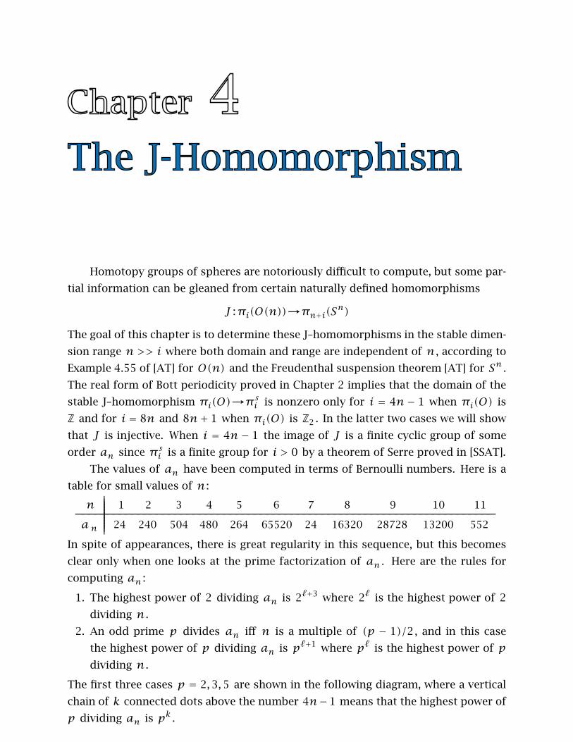
Homotopy groups of spheres are notoriously difficult to compute, but some par-
tial information can be gleaned from certain naturally defined homomorphisms
J :πi(O(n))→πn+i(Sn)
The goal of this chapter is to determine these J–homomorphisms in the stable dimen-
sion range n >> i where both domain and range are independent of n , according to
Example 4.55 of [AT] for O(n) and the Freudenthal suspension theorem [AT] for Sn .
The real form of Bott periodicity proved in Chapter 2 implies that the domain of the
stable J–homomorphism πi(O)→π si is nonzero only for i = 4n− 1 when πi(O) is
Z and for i = 8n and 8n+ 1 when πi(O) is Z2 . In the latter two cases we will show
that J is injective. When i = 4n − 1 the image of J is a finite cyclic group of some
order an since π si is a finite group for i > 0 by a theorem of Serre proved in [SSAT].
The values of an have been computed in terms of Bernoulli numbers. Here is a
table for small values of n :
In spite of appearances, there is great regularity in this sequence, but this becomes
clear only when one looks at the prime factorization of an . Here are the rules for
computing an :
1. The highest power of 2 dividing an is 2ℓ+3 where 2ℓ is the highest power of 2
dividing n .
2. An odd prime p divides an iff n is a multiple of (p − 1)/2, and in this case
the highest power of p dividing an is pℓ+1 where pℓ is the highest power of p
dividing n .
The first three cases p = 2,3,5 are shown in the following diagram, where a vertical
chain of k connected dots above the number 4n−1 means that the highest power of
p dividing an is pk .
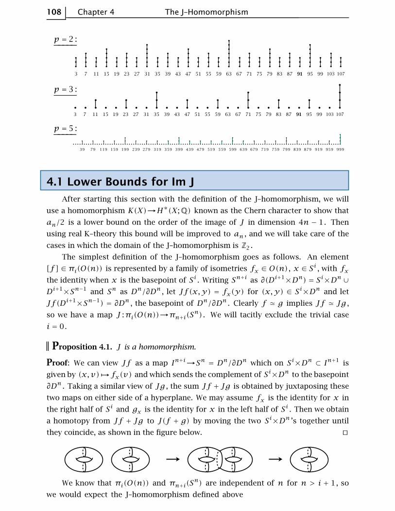
108 Chapter 4 The J–Homomorphism
4.1 Lower Bounds for Im J
After starting this section with the definition of the J–homomorphism, we will
use a homomorphism K(X)→H∗(X;Q) known as the Chern character to show that
an/2 is a lower bound on the order of the image of J in dimension 4n − 1. Then
using real K–theory this bound will be improved to an , and we will take care of the
cases in which the domain of the J–homomorphism is Z2 .
The simplest definition of the J–homomorphism goes as follows. An element
[f ] ∈ πi(O(n)) is represented by a family of isometries fx ∈ O(n) , x ∈ Si , with fx
the identity when x is the basepoint of Si . Writing Sn+i as ∂(Di+1×Dn) = Si×Dn ∪
Di+1×Sn−1 and Sn as Dn/∂Dn , let Jf(x,y) = fx(y) for (x,y) ∈ Si×Dn and let
Jf(Di+1×Sn−1) = ∂Dn , the basepoint of Dn/∂Dn . Clearly f ≃ g implies Jf ≃ Jg ,
so we have a map J :πi(O(n))→πn+i(Sn) . We will tacitly exclude the trivial case
i = 0.
Proposition 4.1. J is a homomorphism.
Proof: We can view Jf as a map In+i→Sn = Dn/∂Dn which on Si×Dn ⊂ In+1 is
given by (x,v)֏fx(v) and which sends the complement of Si×Dn to the basepoint
∂Dn . Taking a similar view of Jg , the sum Jf + Jg is obtained by juxtaposing these
two maps on either side of a hyperplane. We may assume fx is the identity for x in
the right half of Si and gx is the identity for x in the left half of Si . Then we obtain
a homotopy from Jf + Jg to J(f + g) by moving the two Si×Dn ’s together until
they coincide, as shown in the figure below. ⊔⊓
¡¡→ ¡¡→We know that πi(O(n)) and πn+i(S
n) are independent of n for n > i + 1, so
we would expect the J–homomorphism defined above
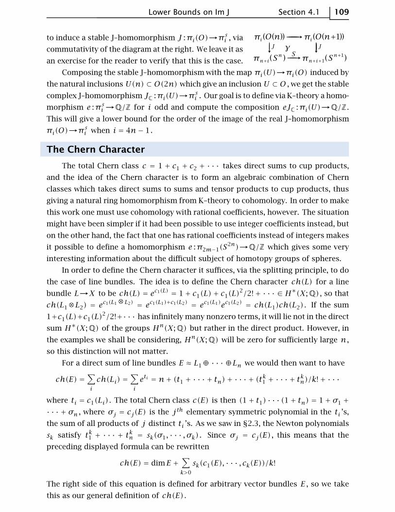
Lower Bounds on Im J Section 4.1 109
to induce a stable J–homomorphism J :πi(O)→π si , via
γcommutativity of the diagram at the right. We leave it as
an exercise for the reader to verify that this is the case.
Composing the stable J–homomorphism with the map πi(U)→πi(O) induced by
the natural inclusions U(n) ⊂ O(2n) which give an inclusion U ⊂ O , we get the stable
complex J–homomorphism JC :πi(U)→π si . Our goal is to define via K–theory a homo-
morphism e :π si→Q/Z for i odd and compute the composition eJC :πi(U)→Q/Z .
This will give a lower bound for the order of the image of the real J–homomorphism
πi(O)→π si when i = 4n− 1.
The Chern Character
The total Chern class c = 1 + c1 + c2 + · · · takes direct sums to cup products,
and the idea of the Chern character is to form an algebraic combination of Chern
classes which takes direct sums to sums and tensor products to cup products, thus
giving a natural ring homomorphism from K–theory to cohomology. In order to make
this work one must use cohomology with rational coefficients, however. The situation
might have been simpler if it had been possible to use integer coefficients instead, but
on the other hand, the fact that one has rational coefficients instead of integers makes
it possible to define a homomorphism e :π2m−1(S2n)→Q/Z which gives some very
interesting information about the difficult subject of homotopy groups of spheres.
In order to define the Chern character it suffices, via the splitting principle, to do
the case of line bundles. The idea is to define the Chern character ch(L) for a line
bundle L→X to be ch(L) = ec1(L) = 1+ c1(L)+ c1(L)2/2!+ · · · ∈ H∗(X;Q) , so that
ch(L1⊗L2) = ec1(L1⊗L2) = ec1(L1)+c1(L2) = ec1(L1)ec1(L2) = ch(L1)ch(L2) . If the sum
1+c1(L)+c1(L)2/2!+· · · has infinitely many nonzero terms, it will lie not in the direct
sum H∗(X;Q) of the groups Hn(X;Q) but rather in the direct product. However, in
the examples we shall be considering, Hn(X;Q) will be zero for sufficiently large n ,
so this distinction will not matter.
For a direct sum of line bundles E ≈ L1⊕ · · · ⊕Ln we would then want to have
ch(E) =∑
i
ch(Li) =∑
i
eti = n+ (t1 + · · · + tn)+ · · · + (tk1 + · · · + t
kn)/k!+ · · ·
where ti = c1(Li) . The total Chern class c(E) is then (1+ t1) · · · (1+ tn) = 1+ σ1 +
· · · + σn , where σj = cj(E) is the j th elementary symmetric polynomial in the ti ’s,
the sum of all products of j distinct ti ’s. As we saw in §2.3, the Newton polynomials
sk satisfy tk1 + · · · + tkn = sk(σ1, · · · , σk) . Since σj = cj(E) , this means that the
preceding displayed formula can be rewritten
ch(E) = dimE +∑
k>0
sk(c1(E), · · · , ck(E))/k!
The right side of this equation is defined for arbitrary vector bundles E , so we take
this as our general definition of ch(E) .
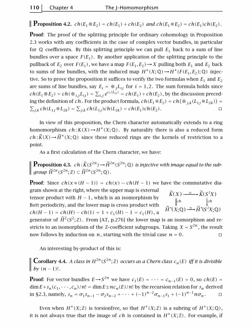
110 Chapter 4 The J–Homomorphism
Proposition 4.2. ch(E1⊕E2) = ch(E1)+ ch(E2) and ch(E1⊗E2) = ch(E1)ch(E2) .
Proof: The proof of the splitting principle for ordinary cohomology in Proposition
2.3 works with any coefficients in the case of complex vector bundles, in particular
for Q coefficients. By this splitting principle we can pull E1 back to a sum of line
bundles over a space F(E1) . By another application of the splitting principle to the
pullback of E2 over F(E1) , we have a map F(E1, E2)→X pulling both E1 and E2 back
to sums of line bundles, with the induced map H∗(X;Q)→H∗(F(E1, E2);Q) injec-
tive. So to prove the proposition it suffices to verify the two formulas when E1 and E2
are sums of line bundles, say Ei = ⊕jLij for i = 1,2. The sum formula holds since
ch(E1⊕E2) = ch(⊕ i,jLij) =∑i,j e
c1(Lij) = ch(E1)+ch(E2) , by the discussion preced-
ing the definition of ch . For the product formula, ch(E1⊗E2) = ch(⊕ j,k(L1j⊗L2k)
)=∑
j,k ch(L1j⊗L2k) =∑j,k ch(L1j)ch(L2k) = ch(E1)ch(E2) . ⊔⊓
In view of this proposition, the Chern character automatically extends to a ring
homomorphism ch :K(X)→H∗(X;Q) . By naturality there is also a reduced form
ch : K(X)→H∗(X;Q) since these reduced rings are the kernels of restriction to a
point.
As a first calculation of the Chern character, we have:
Proposition 4.3. ch : K(S2n)→H2n(S2n;Q) is injective with image equal to the sub-
group H2n(S2n;Z) ⊂ H2n(S2n;Q) .
Proof: Since ch(x ⊗ (H − 1)) = ch(x) ` ch(H − 1) we have the commutative dia-
gram shown at the right, where the upper map is external
tensor product with H − 1, which is an isomorphism by
Bott periodicity, and the lower map is cross product with
ch(H − 1) = ch(H) − ch(1) = 1 + c1(H) − 1 = c1(H) , a
generator of H2(S2;Z) . From [AT, p.276] the lower map is an isomorphism and re-
stricts to an isomorphism of the Z coefficient subgroups. Taking X = S2n , the result
now follows by induction on n , starting with the trivial case n = 0. ⊔⊓
An interesting by-product of this is:
Corollary 4.4. A class in H2n(S2n;Z) occurs as a Chern class cn(E) iff it is divisible
by (n− 1)! .
Proof: For vector bundles E→S2n we have c1(E) = · · · = cn−1(E) = 0, so ch(E) =
dimE+sn(c1, · · · , cn)/n! = dimE±ncn(E)/n! by the recursion relation for sn derived
in §2.3, namely, sn = σ1sn−1 − σ2sn−2 + · · · + (−1)n−2σn−1s1 + (−1)n−1nσn . ⊔⊓
Even when H∗(X;Z) is torsionfree, so that H∗(X;Z) is a subring of H∗(X;Q) ,
it is not always true that the image of ch is contained in H∗(X;Z) . For example, if
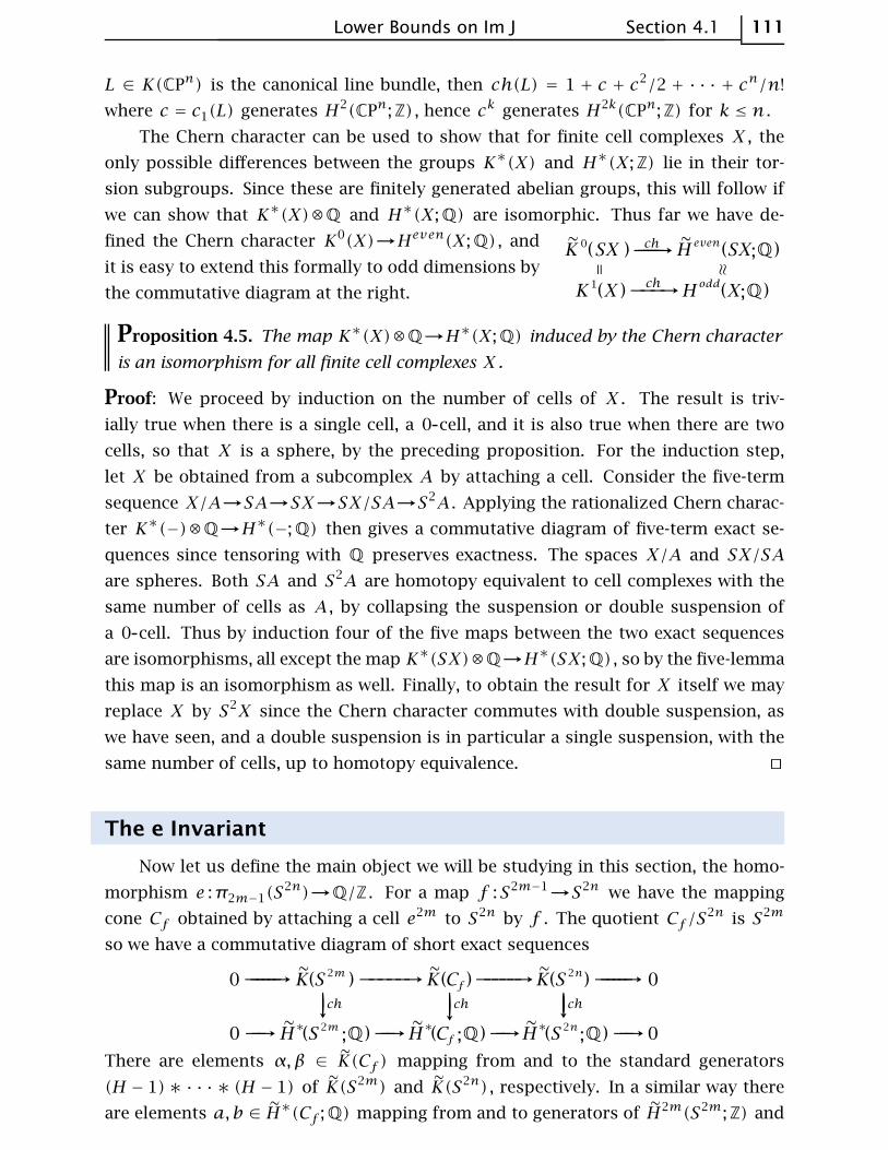
Lower Bounds on Im J Section 4.1 111
L ∈ K(CPn) is the canonical line bundle, then ch(L) = 1 + c + c2/2 + · · · + cn/n!
where c = c1(L) generates H2(CPn;Z) , hence ck generates H2k(CPn;Z) for k ≤ n .
The Chern character can be used to show that for finite cell complexes X , the
only possible differences between the groups K∗(X) and H∗(X;Z) lie in their tor-
sion subgroups. Since these are finitely generated abelian groups, this will follow if
we can show that K∗(X)⊗Q and H∗(X;Q) are isomorphic. Thus far we have de-
fined the Chern character K0(X)→Heven(X;Q) , and
it is easy to extend this formally to odd dimensions by
the commutative diagram at the right.
Proposition 4.5. The map K∗(X)⊗Q→H∗(X;Q) induced by the Chern character
is an isomorphism for all finite cell complexes X .
Proof: We proceed by induction on the number of cells of X . The result is triv-
ially true when there is a single cell, a 0 cell, and it is also true when there are two
cells, so that X is a sphere, by the preceding proposition. For the induction step,
let X be obtained from a subcomplex A by attaching a cell. Consider the five-term
sequence X/A→SA→SX→SX/SA→S2A . Applying the rationalized Chern charac-
ter K∗(−)⊗Q→H∗(−;Q) then gives a commutative diagram of five-term exact se-
quences since tensoring with Q preserves exactness. The spaces X/A and SX/SA
are spheres. Both SA and S2A are homotopy equivalent to cell complexes with the
same number of cells as A , by collapsing the suspension or double suspension of
a 0 cell. Thus by induction four of the five maps between the two exact sequences
are isomorphisms, all except the map K∗(SX)⊗Q→H∗(SX;Q) , so by the five-lemma
this map is an isomorphism as well. Finally, to obtain the result for X itself we may
replace X by S2X since the Chern character commutes with double suspension, as
we have seen, and a double suspension is in particular a single suspension, with the
same number of cells, up to homotopy equivalence. ⊔⊓
The e Invariant
Now let us define the main object we will be studying in this section, the homo-
morphism e :π2m−1(S2n)→Q/Z . For a map f :S2m−1→S2n we have the mapping
cone Cf obtained by attaching a cell e2m to S2n by f . The quotient Cf /S2n is S2m
so we have a commutative diagram of short exact sequences
There are elements α,β ∈ K(Cf ) mapping from and to the standard generators
(H − 1)∗ · · · ∗ (H − 1) of K(S2m) and K(S2n) , respectively. In a similar way there
are elements a,b ∈ H∗(Cf ;Q) mapping from and to generators of H2m(S2m;Z) and
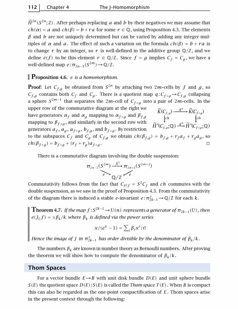
112 Chapter 4 The J–Homomorphism
H2n(S2n;Z) . After perhaps replacing a and b by their negatives we may assume that
ch(α) = a and ch(β) = b+ ra for some r ∈ Q , using Proposition 4.3. The elements
β and b are not uniquely determined but can be varied by adding any integer mul-
tiples of α and a . The effect of such a variation on the formula ch(β) = b + ra is
to change r by an integer, so r is well-defined in the additive group Q/Z , and we
define e(f) to be this element r ∈ Q/Z . Since f ≃ g implies Cf ≃ Cg , we have a
well-defined map e :π2n−1(S2m)→Q/Z .
Proposition 4.6. e is a homomorphism.
Proof: Let Cf ,g be obtained from S2n by attaching two 2m cells by f and g , so
Cf ,g contains both Cf and Cg . There is a quotient map q :Cf+g→Cf ,g collapsing
a sphere S2m−1 that separates the 2m cell of Cf+g into a pair of 2m cells. In the
upper row of the commutative diagram at the right we
have generators αf and αg mapping to αf+g and βf ,gmapping to βf+g , and similarly in the second row with
generators af , ag , af+g , bf ,g , and bf+g . By restriction
to the subspaces Cf and Cg of Cf ,g we obtain ch(βf ,g) = bf ,g + rfaf + rgag , so
ch(βf+g) = bf+g + (rf + rg)af+g . ⊔⊓
There is a commutative diagram involving the double suspension:
Commutativity follows from the fact that CS2f = S2Cf and ch commutes with the
double suspension, as we saw in the proof of Proposition 4.3. From the commutativity
of the diagram there is induced a stable e invariant e :π s2k−1→Q/Z for each k .
Theorem 4.7. If the map f :S2k−1→U(n) represents a generator of π2k−1(U) , then
e(JCf) = ±βk/k where βk is defined via the power series
x/(ex − 1) =∑iβix
i/i!
Hence the image of J in π s2k−1 has order divisible by the denominator of βk/k .
The numbers βk are known in number theory as Bernoulli numbers. After proving
the theorem we will show how to compute the denominator of βk/k .
Thom Spaces
For a vector bundle E→B with unit disk bundle D(E) and unit sphere bundle
S(E) the quotient space D(E)/S(E) is called the Thom space T(E) . When B is compact
this can also be regarded as the one-point compactification of E . Thom spaces arise
in the present context through the following:
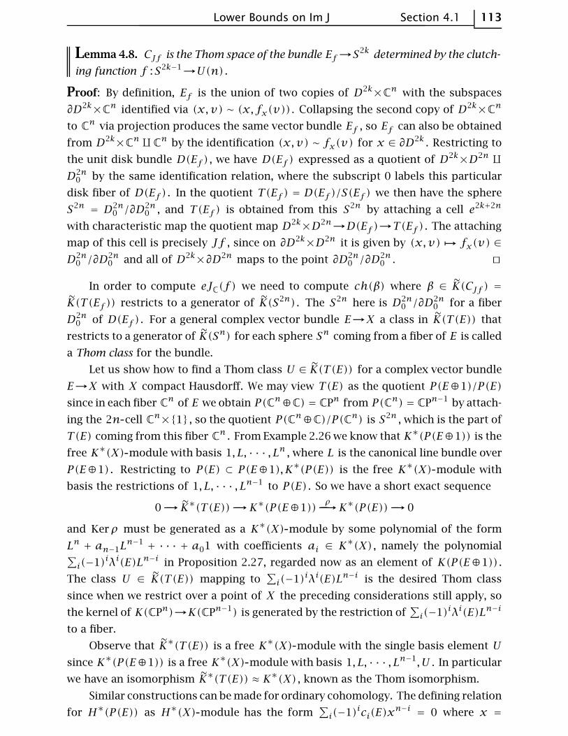
Lower Bounds on Im J Section 4.1 113
Lemma 4.8. CJf is the Thom space of the bundle Ef→S2k determined by the clutch-
ing function f :S2k−1→U(n) .
Proof: By definition, Ef is the union of two copies of D2k×Cn with the subspaces
∂D2k×Cn identified via (x,v) ∼ (x, fx(v)) . Collapsing the second copy of D2k×Cn
to Cn via projection produces the same vector bundle Ef , so Ef can also be obtained
from D2k×Cn∐Cn by the identification (x,v) ∼ fx(v) for x ∈ ∂D2k . Restricting to
the unit disk bundle D(Ef ) , we have D(Ef ) expressed as a quotient of D2k×D2n ∐
D2n0 by the same identification relation, where the subscript 0 labels this particular
disk fiber of D(Ef ) . In the quotient T(Ef ) = D(Ef )/S(Ef ) we then have the sphere
S2n = D2n0 /∂D
2n0 , and T(Ef ) is obtained from this S2n by attaching a cell e2k+2n
with characteristic map the quotient map D2k×D2n→D(Ef )→T(Ef ) . The attaching
map of this cell is precisely Jf , since on ∂D2k×D2n it is given by (x,v)֏ fx(v) ∈
D2n0 /∂D
2n0 and all of D2k×∂D2n maps to the point ∂D2n
0 /∂D2n0 . ⊔⊓
In order to compute eJC(f ) we need to compute ch(β) where β ∈ K(CJf ) =
K(T(Ef )) restricts to a generator of K(S2n) . The S2n here is D2n0 /∂D
2n0 for a fiber
D2n0 of D(Ef ) . For a general complex vector bundle E→X a class in K(T(E)) that
restricts to a generator of K(Sn) for each sphere Sn coming from a fiber of E is called
a Thom class for the bundle.
Let us show how to find a Thom class U ∈ K(T(E)) for a complex vector bundle
E→X with X compact Hausdorff. We may view T(E) as the quotient P(E⊕1)/P(E)
since in each fiber Cn of E we obtain P(Cn⊕C) = CPn from P(Cn) = CPn−1 by attach-
ing the 2n cell Cn×{1} , so the quotient P(Cn⊕C)/P(Cn) is S2n , which is the part of
T(E) coming from this fiber Cn . From Example 2.26 we know that K∗(P(E⊕1)) is the
free K∗(X) module with basis 1, L, · · · , Ln , where L is the canonical line bundle over
P(E⊕1) . Restricting to P(E) ⊂ P(E⊕1),K∗(P(E)) is the free K∗(X) module with
basis the restrictions of 1, L, · · · , Ln−1 to P(E) . So we have a short exact sequence
0 -→ K∗(T(E)) -→K∗(P(E⊕1))ρ-----→K∗(P(E)) -→0
and Kerρ must be generated as a K∗(X) module by some polynomial of the form
Ln + an−1Ln−1 + · · · + a01 with coefficients ai ∈ K
∗(X) , namely the polynomial∑i(−1)iλi(E)Ln−i in Proposition 2.27, regarded now as an element of K(P(E⊕1)) .
The class U ∈ K(T(E)) mapping to∑i(−1)iλi(E)Ln−i is the desired Thom class
since when we restrict over a point of X the preceding considerations still apply, so
the kernel of K(CPn)→K(CPn−1) is generated by the restriction of∑i(−1)iλi(E)Ln−i
to a fiber.
Observe that K∗(T(E)) is a free K∗(X) module with the single basis element U
since K∗(P(E⊕1)) is a free K∗(X) module with basis 1, L, · · · , Ln−1, U . In particular
we have an isomorphism K∗(T(E)) ≈ K∗(X) , known as the Thom isomorphism.
Similar constructions can be made for ordinary cohomology. The defining relation
for H∗(P(E)) as H∗(X) module has the form∑i(−1)ici(E)x
n−i = 0 where x =
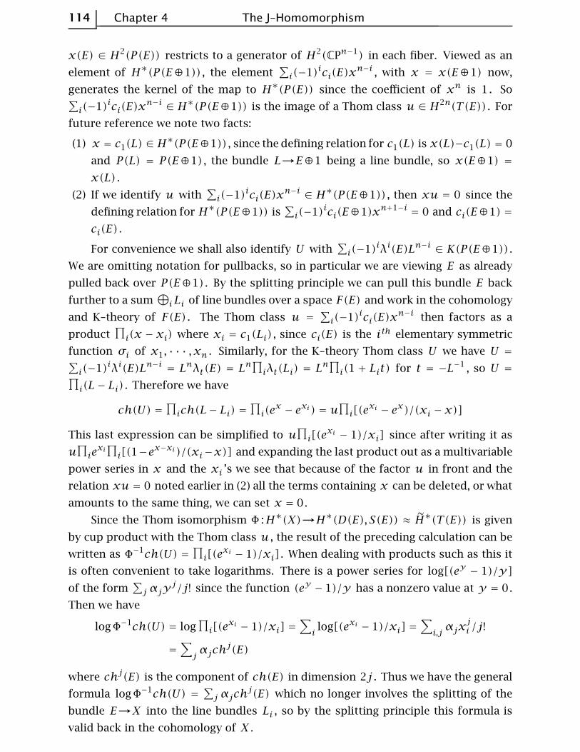
114 Chapter 4 The J–Homomorphism
x(E) ∈ H2(P(E)) restricts to a generator of H2(CPn−1) in each fiber. Viewed as an
element of H∗(P(E⊕1)) , the element∑i(−1)ici(E)x
n−i , with x = x(E⊕1) now,
generates the kernel of the map to H∗(P(E)) since the coefficient of xn is 1. So∑i(−1)ici(E)x
n−i ∈ H∗(P(E⊕1)) is the image of a Thom class u ∈ H2n(T(E)) . For
future reference we note two facts:
(1) x = c1(L) ∈ H∗(P(E⊕1)) , since the defining relation for c1(L) is x(L)−c1(L) = 0
and P(L) = P(E⊕1) , the bundle L→E⊕1 being a line bundle, so x(E⊕1) =
x(L) .
(2) If we identify u with∑i(−1)ici(E)x
n−i ∈ H∗(P(E⊕1)) , then xu = 0 since the
defining relation for H∗(P(E⊕1)) is∑i(−1)ici(E⊕1)xn+1−i = 0 and ci(E⊕1) =
ci(E) .
For convenience we shall also identify U with∑i(−1)iλi(E)Ln−i ∈ K(P(E⊕1)) .
We are omitting notation for pullbacks, so in particular we are viewing E as already
pulled back over P(E⊕1) . By the splitting principle we can pull this bundle E back
further to a sum⊕iLi of line bundles over a space F(E) and work in the cohomology
and K–theory of F(E) . The Thom class u =∑i(−1)ici(E)x
n−i then factors as a
product∏i(x − xi) where xi = c1(Li) , since ci(E) is the ith elementary symmetric
function σi of x1, · · · , xn . Similarly, for the K–theory Thom class U we have U =∑i(−1)iλi(E)Ln−i = Lnλt(E) = L
n∏iλt(Li) = L
n∏i(1 + Lit) for t = −L−1 , so U =∏
i(L− Li) . Therefore we have
ch(U) =∏ich(L− Li) =
∏i(e
x − exi) = u∏i[(e
xi − ex)/(xi − x)]
This last expression can be simplified to u∏i[(e
xi − 1)/xi] since after writing it as
u∏iexi∏i[(1−e
x−xi)/(xi−x)] and expanding the last product out as a multivariable
power series in x and the xi ’s we see that because of the factor u in front and the
relation xu = 0 noted earlier in (2) all the terms containing x can be deleted, or what
amounts to the same thing, we can set x = 0.
Since the Thom isomorphism Φ :H∗(X)→H∗(D(E), S(E)) ≈ H∗(T(E)) is given
by cup product with the Thom class u , the result of the preceding calculation can be
written as Φ−1ch(U) =∏i[(e
xi − 1)/xi] . When dealing with products such as this it
is often convenient to take logarithms. There is a power series for log[(ey − 1)/y]
of the form∑j αjy
j/j! since the function (ey − 1)/y has a nonzero value at y = 0.
Then we have
logΦ−1ch(U) = log∏i[(e
xi − 1)/xi] =∑ilog[(exi − 1)/xi] =
∑i,jαjx
ji /j!
=∑jαjch
j(E)
where chj(E) is the component of ch(E) in dimension 2j . Thus we have the general
formula logΦ−1ch(U) =∑j αjch
j(E) which no longer involves the splitting of the
bundle E→X into the line bundles Li , so by the splitting principle this formula is
valid back in the cohomology of X .
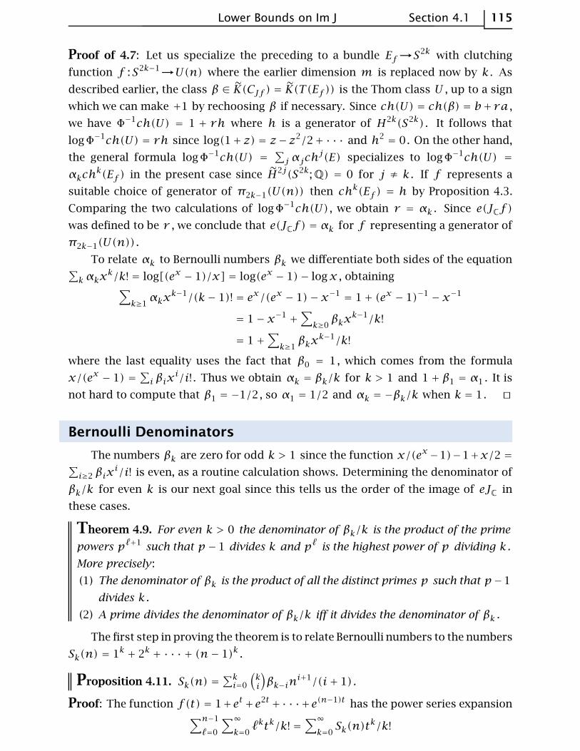
Lower Bounds on Im J Section 4.1 115
Proof of 4.7: Let us specialize the preceding to a bundle Ef→S2k with clutching
function f :S2k−1→U(n) where the earlier dimension m is replaced now by k . As
described earlier, the class β ∈ K(CJf ) = K(T(Ef )) is the Thom class U , up to a sign
which we can make +1 by rechoosing β if necessary. Since ch(U) = ch(β) = b+ra ,
we have Φ−1ch(U) = 1 + rh where h is a generator of H2k(S2k) . It follows that
logΦ−1ch(U) = rh since log(1+z) = z−z2/2+· · · and h2 = 0. On the other hand,
the general formula logΦ−1ch(U) =∑j αjch
j(E) specializes to logΦ−1ch(U) =
αkchk(Ef ) in the present case since H2j(S2k;Q) = 0 for j ≠ k . If f represents a
suitable choice of generator of π2k−1(U(n)) then chk(Ef ) = h by Proposition 4.3.
Comparing the two calculations of logΦ−1ch(U) , we obtain r = αk . Since e(JCf)
was defined to be r , we conclude that e(JCf) = αk for f representing a generator of
π2k−1(U(n)) .
To relate αk to Bernoulli numbers βk we differentiate both sides of the equation∑kαkx
k/k! = log[(ex − 1)/x] = log(ex − 1)− logx , obtaining∑k≥1αkx
k−1/(k− 1)! = ex/(ex − 1)− x−1 = 1+ (ex − 1)−1 − x−1
= 1− x−1 +∑k≥0βkx
k−1/k!
= 1+∑k≥1βkx
k−1/k!
where the last equality uses the fact that β0 = 1, which comes from the formula
x/(ex − 1) =∑i βix
i/i! . Thus we obtain αk = βk/k for k > 1 and 1+ β1 = α1 . It is
not hard to compute that β1 = −1/2, so α1 = 1/2 and αk = −βk/k when k = 1. ⊔⊓
Bernoulli Denominators
The numbers βk are zero for odd k > 1 since the function x/(ex−1)−1+x/2 =∑i≥2 βix
i/i! is even, as a routine calculation shows. Determining the denominator of
βk/k for even k is our next goal since this tells us the order of the image of eJC in
these cases.
Theorem 4.9. For even k > 0 the denominator of βk/k is the product of the prime
powers pℓ+1 such that p−1 divides k and pℓ is the highest power of p dividing k .
More precisely :
(1) The denominator of βk is the product of all the distinct primes p such that p−1
divides k .
(2) A prime divides the denominator of βk/k iff it divides the denominator of βk .
The first step in proving the theorem is to relate Bernoulli numbers to the numbers
Sk(n) = 1k + 2k + · · · + (n− 1)k .
Proposition 4.11. Sk(n) =∑ki=0
(ki
)βk−in
i+1/(i+ 1) .
Proof: The function f(t) = 1+et+e2t +· · ·+e(n−1)t has the power series expansion∑n−1
ℓ=0
∑∞
k=0ℓktk/k! =
∑∞
k=0Sk(n)t
k/k!
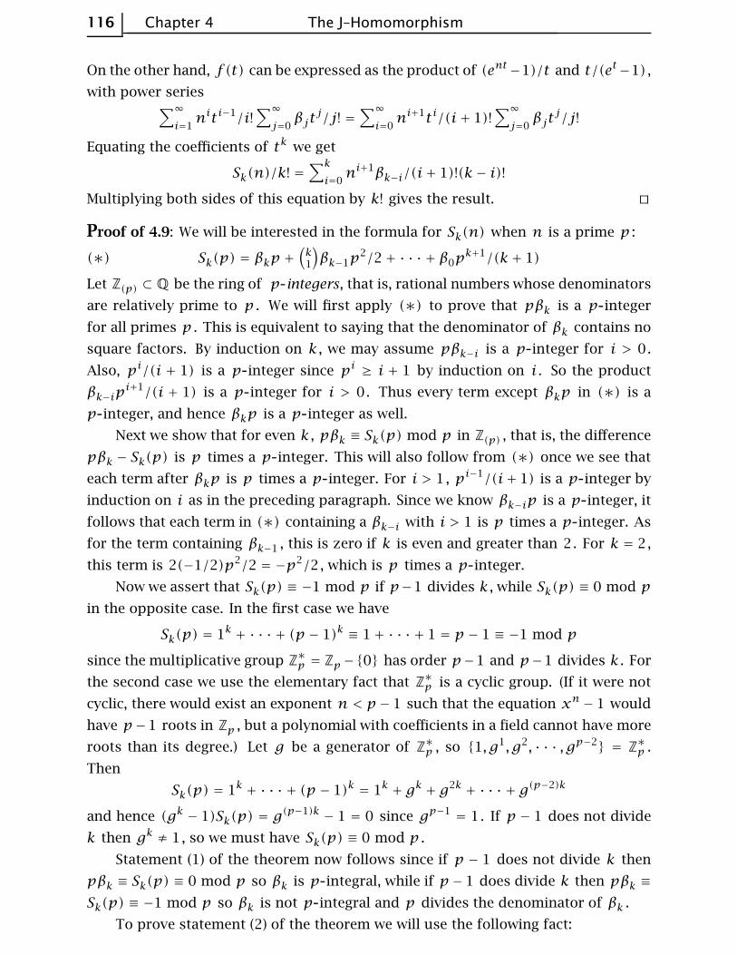
116 Chapter 4 The J–Homomorphism
On the other hand, f(t) can be expressed as the product of (ent−1)/t and t/(et−1) ,
with power series∑∞
i=1niti−1/i!
∑∞
j=0βjt
j/j! =∑∞
i=0ni+1ti/(i+ 1)!
∑∞
j=0βjt
j/j!
Equating the coefficients of tk we get
Sk(n)/k! =∑k
i=0ni+1βk−i/(i+ 1)!(k− i)!
Multiplying both sides of this equation by k! gives the result. ⊔⊓
Proof of 4.9: We will be interested in the formula for Sk(n) when n is a prime p :
(∗) Sk(p) = βkp +(k1
)βk−1p
2/2+ · · · + β0pk+1/(k+ 1)
Let Z(p) ⊂ Q be the ring of p integers, that is, rational numbers whose denominators
are relatively prime to p . We will first apply (∗) to prove that pβk is a p integer
for all primes p . This is equivalent to saying that the denominator of βk contains no
square factors. By induction on k , we may assume pβk−i is a p integer for i > 0.
Also, pi/(i + 1) is a p integer since pi ≥ i + 1 by induction on i . So the product
βk−ipi+1/(i + 1) is a p integer for i > 0. Thus every term except βkp in (∗) is a
p integer, and hence βkp is a p integer as well.
Next we show that for even k , pβk ≡ Sk(p) mod p in Z(p) , that is, the difference
pβk − Sk(p) is p times a p integer. This will also follow from (∗) once we see that
each term after βkp is p times a p integer. For i > 1, pi−1/(i+ 1) is a p integer by
induction on i as in the preceding paragraph. Since we know βk−ip is a p integer, it
follows that each term in (∗) containing a βk−i with i > 1 is p times a p integer. As
for the term containing βk−1 , this is zero if k is even and greater than 2. For k = 2,
this term is 2(−1/2)p2/2 = −p2/2, which is p times a p integer.
Now we assert that Sk(p) ≡ −1 mod p if p−1 divides k , while Sk(p) ≡ 0 mod p
in the opposite case. In the first case we have
Sk(p) = 1k + · · · + (p − 1)k ≡ 1+ · · · + 1 = p − 1 ≡ −1 mod p
since the multiplicative group Z∗p = Zp−{0} has order p−1 and p−1 divides k . For
the second case we use the elementary fact that Z∗p is a cyclic group. (If it were not
cyclic, there would exist an exponent n < p− 1 such that the equation xn − 1 would
have p−1 roots in Zp , but a polynomial with coefficients in a field cannot have more
roots than its degree.) Let g be a generator of Z∗p , so {1, g1, g2, · · · , gp−2} = Z∗p .
Then
Sk(p) = 1k + · · · + (p − 1)k = 1k + gk + g2k + · · · + g(p−2)k
and hence (gk − 1)Sk(p) = g(p−1)k − 1 = 0 since gp−1 = 1. If p − 1 does not divide
k then gk ≠ 1, so we must have Sk(p) ≡ 0 mod p .
Statement (1) of the theorem now follows since if p − 1 does not divide k then
pβk ≡ Sk(p) ≡ 0 mod p so βk is p integral, while if p− 1 does divide k then pβk ≡
Sk(p) ≡ −1 mod p so βk is not p integral and p divides the denominator of βk .
To prove statement (2) of the theorem we will use the following fact:
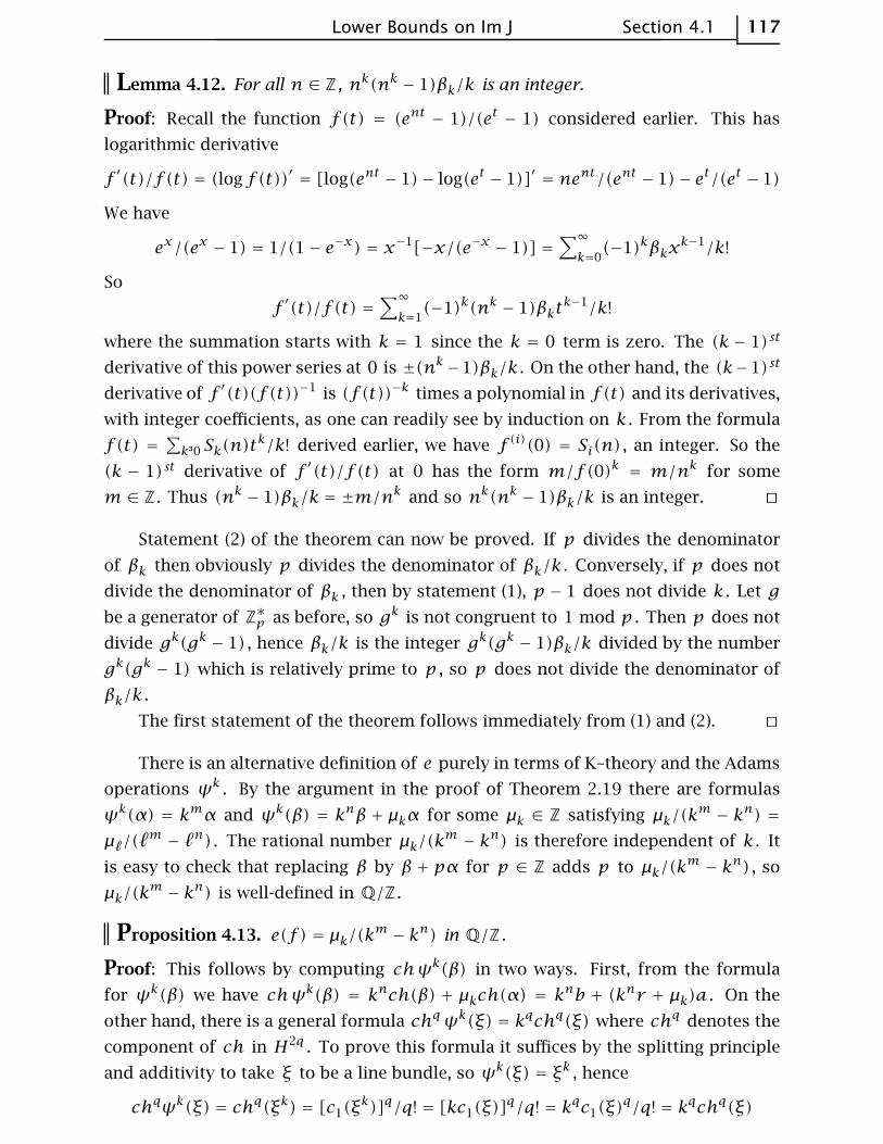
Lower Bounds on Im J Section 4.1 117
Lemma 4.12. For all n ∈ Z , nk(nk − 1)βk/k is an integer.
Proof: Recall the function f(t) = (ent − 1)/(et − 1) considered earlier. This has
logarithmic derivative
f ′(t)/f(t) = (log f(t))′ = [log(ent − 1)− log(et − 1)]′ = nent/(ent − 1)− et/(et − 1)
We have
ex/(ex − 1) = 1/(1− e−x) = x−1[−x/(e−x − 1)] =∑∞
k=0(−1)kβkx
k−1/k!
So
f ′(t)/f(t) =∑∞
k=1(−1)k(nk − 1)βkt
k−1/k!
where the summation starts with k = 1 since the k = 0 term is zero. The (k − 1)st
derivative of this power series at 0 is ±(nk−1)βk/k . On the other hand, the (k−1)st
derivative of f ′(t)(f (t))−1 is (f (t))−k times a polynomial in f(t) and its derivatives,
with integer coefficients, as one can readily see by induction on k . From the formula
f(t) =∑k³0 Sk(n)t
k/k! derived earlier, we have f (i)(0) = Si(n) , an integer. So the
(k − 1)st derivative of f ′(t)/f(t) at 0 has the form m/f(0)k = m/nk for some
m ∈ Z . Thus (nk − 1)βk/k = ±m/nk and so nk(nk − 1)βk/k is an integer. ⊔⊓
Statement (2) of the theorem can now be proved. If p divides the denominator
of βk then obviously p divides the denominator of βk/k . Conversely, if p does not
divide the denominator of βk , then by statement (1), p − 1 does not divide k . Let g
be a generator of Z∗p as before, so gk is not congruent to 1 mod p . Then p does not
divide gk(gk − 1) , hence βk/k is the integer gk(gk − 1)βk/k divided by the number
gk(gk − 1) which is relatively prime to p , so p does not divide the denominator of
βk/k .
The first statement of the theorem follows immediately from (1) and (2). ⊔⊓
There is an alternative definition of e purely in terms of K–theory and the Adams
operations ψk . By the argument in the proof of Theorem 2.19 there are formulas
ψk(α) = kmα and ψk(β) = knβ + µkα for some µk ∈ Z satisfying µk/(km − kn) =
µℓ/(ℓm − ℓn) . The rational number µk/(k
m − kn) is therefore independent of k . It
is easy to check that replacing β by β + pα for p ∈ Z adds p to µk/(km − kn) , so
µk/(km − kn) is well-defined in Q/Z .
Proposition 4.13. e(f) = µk/(km − kn) in Q/Z .
Proof: This follows by computing chψk(β) in two ways. First, from the formula
for ψk(β) we have chψk(β) = knch(β) + µkch(α) = knb + (knr + µk)a . On the
other hand, there is a general formula chqψk(ξ) = kqchq(ξ) where chq denotes the
component of ch in H2q . To prove this formula it suffices by the splitting principle
and additivity to take ξ to be a line bundle, so ψk(ξ) = ξk , hence
chqψk(ξ) = chq(ξk) = [c1(ξk)]q/q! = [kc1(ξ)]
q/q! = kqc1(ξ)q/q! = kqchq(ξ)
118 Chapter 4 The J–Homomorphism
In the case at hand this says chmψk(β) = kmchm(β) = kmra . Comparing this with
the coefficient of a in the first formula for chψk(β) gives µk = r(km − kn) . ⊔⊓
Books
M. F. Atiyah, K–Theory, W. A. Benjamin, 1967.
R. Bott, Lectures on K(X), W. A. Benjamin, 1969.
J. Dieudonne, A History of Algebraic and Differential Topology 1900-1960, Birkhauser, 1989.
W. Fulton, Young Tableaux, Cambridge Univ. Press, 1997.
H. Hiller, Geometry of Coxeter Groups, Pitman, 1982.
D. Husemoller, Fibre Bundles, McGraw-Hill, 1966 (later editions by Springer-Verlag).
M. Karoubi, K–Theory: An Introduction, Springer-Verlag, 1978.
S. Lang, Algebra, Addison-Wesley, 1965.
J. W. Milnor and J. D. Stasheff, Characteristic Classes, Princeton Univ. Press, 1974.
N. Steenrod, Topology of Fiber Bundles, Princeton Univ. Press, 1951.
R. Stong, Notes on Cobordism Theory, Princeton Univ. Press, 1968.
B. L. van der Waerden, Modern Algebra, Ungar, 1949.
Papers
J. F. Adams, On the non-existence of elements of Hopf invariant one, Ann. of Math. 72 (1960),
20–104.
J. F. Adams, Vector fields on spheres, Ann. of Math. 75 (1962), 603–632.
J. F. Adams, On the groups J(X) IV, Topology 5 (1966), 21–71.
J. F. Adams and M. F. Atiyah, K–theory and the Hopf invariant, Quart. J. Math. 17 (1966),
31–38.
M. Atiyah and F. Hirzebruch, Vector Bundles and Homogeneous Spaces, Proc. Sym. Pure
Math.. III (1961), 7–38.
M. Atiyah, Vector bundles and the Kunneth formula, Topology 1 (1962), 245–248.
M. Atiyah, Power Operations in K–Theory, Quart. J. Math. Oxford. 17 (1966), 165–193.
M. Atiyah, K–Theory and reality, Quart. J. Math. Oxford. 17 (1966), 367–386.
M. Atiyah and R. Bott, On the periodicity theorem for complex vector bundles, Acta Math.
112 (1964), 229–247.
M. Atiyah, R. Bott and A. Shapiro, Clifford Modules, Topology 3 (1964), 3–38.
R. Bott and J. Milnor, On the parallelizability of spheres, Bull. A.M.S. 64 (1958), 87–89.
R. Bott, The stable homotopy of the classical groups, Ann. of Math. 70 (1959), 313–337.
L. Hodgkin, On the K–Theory of Lie groups, Topology. 6 (1967), 1–36.
M. Mahowald, The order of the image of the J–homomorphism, Bull. A.M.S. 76 (1970), 1310–
1313.
120 Bibliography
J. Milnor, Some consequences of a theorem of Bott, Ann. of Math. 68 (1958), 444–449.
D. Quillen, The Adams conjecture, Topology 10 (1971), 67–80.
D. Sullivan, Genetics of homotopy theory and the Adams conjecture, Ann. of Math. 100 (1974),
1–79.
L. M. Woodward, Vector fields on spheres and a generalization, Quart. J. Math. Oxford. 24
(1973), 357–366.