
Algoritmos Geneticos Guia y Teoria
345
-
Upload
cesarpineda -
Category
Documents
-
view
30 -
download
1
Transcript of Algoritmos Geneticos Guia y Teoria


Genetic Algorithms: Principles and Perspectives
A Guide to GA Theory

OPERATIONS RESEARCH/COMPUTER SCIENCEINTERFACES SERIES
Series Editors
Professor Ramesh ShardaOklahoma State University
Prof. Dr. Stefan VoßTechnische Universität Braunschweig
Other published titles in the series:
Greenberg, Harvey J. / A Computer-Assisted Analysis System for Mathematical ProgrammingModels and Solutions; A User’s Guide for ANALYZE
Greenberg, Harvey J. / Modeling by Object-Driven Linear Elemental Relations: A Users Guide forMODLER
Brown, Donald/Scherer, William T. / Intelligent Scheduling Systems
Nash, Stephen G./Sofer, Ariela / The Impact of Emerging Technologies on ComputerScience & Operations Research
Barth, Peter / Logic-Based 0-1 Constraint ProgrammingJones, Christopher V. / Visualization and OptimizationBarr, Richard S./ Helgason, Richard V./ Kennington, Jeffery L. / Interfaces in Computer
Science & Operations Research: Advances in Metaheuristics, Optimization, & Stochastic ModelingTechnologies
Ellacott, Stephen W./ Mason, John C./ Anderson, Iain J. / Mathematics of Neural Networks:Models, Algorithms & Applications
Woodruff, David L. / Advances in Computational & Stochastic Optimization, Logic Programming,and Heuristic Search
Klein, Robert / Scheduling of Resource-Constrained ProjectsBierwirth, Christian / Adaptive Search and the Management of Logistics SystemsLaguna, Manuel / González-Velarde, José Luis / Computing Tools for Modeling, Optimization
and SimulationStilman, Boris / Linguistic Geometry: From Search to Construction
Sakawa, Masatoshi / Genetic Algorithms and Fuzzy Multiobjective OptimizationRibeiro, Celso C./ Hansen, Pierre / Essays and Surveys in MetaheuristicsHolsapple, Clyde/ Jacob, Varghese / Rao, H. R. / BUSINESS MODELLING: Multidisciplinary
Approaches — Economics, Operational and Information Systems PerspectivesSleezer, Catherine M./ Wentling, Tim L./ Cude, Roger L. / HUMAN RESOURCE
DEVELOPMENT AND INFORMATION TECHNOLOGY: Making Global ConnectionsVoß, Stefan, Woodruff, David / Optimization Software Class Libraries
Upadhyaya et al/ MOBILE COMPUTING: Implementing Pervasive Information and Communications Technologies
Reeves, Colin & Rowe, Jonathan/ GENETIC ALGORITHMS—Principles and Perspectives: AGuide to GA Theory

GENETIC ALGORITHMS: PRINCIPLES ANDPERSPECTIVES
A Guide to GA Theory
COLIN R.REEVESSchool of Mathematical and Information SciencesCoventry University
JONATHAN E.ROWESchool of Computer ScienceUniversity of Birmingham
KLUWER ACADEMIC PUBLISHERSNEW YORK, BOSTON, DORDRECHT, LONDON, MOSCOW

eBook ISBN: 0-306-48050-6Print ISBN: 1-4020-7240-6
©2002 Kluwer Academic PublishersNew York, Boston, Dordrecht, London, Moscow
Print ©2003 Kluwer Academic Publishers
All rights reserved
No part of this eBook may be reproduced or transmitted in any form or by any means, electronic,mechanical, recording, or otherwise, without written consent from the Publisher
Created in the United States of America
Visit Kluwer Online at: http://kluweronline.comand Kluwer's eBookstore at: http://ebooks.kluweronline.com
Dordrecht

Contents
1
2
3
4
Introduction1.11.21.31.4
Historical Background1149
OptimizationWhy GAs? Why Theory?Bibliographic Notes 17
191919254951555960
656568747884869091
959596
Basic Principles2.12.22.32.42.52.62.72.8
GA ConceptsRepresentationThe Elements of a Genetic AlgorithmIllustrative ExamplePractical ConsiderationsSpecial CasesSummaryBibliographic Notes
Schema Theory3.13.23.33.43.53.63.73.8
SchemataThe Schema TheoremCritiques of Schema-Based TheorySurveying the WreckageExact ModelsWalsh Transforms and deceptionConclusionBibliographic Notes
No Free Lunch for GAs4.14.2
IntroductionThe Theorem

vi CONTENTS
4.34.44.54.6
Developments 103106108109
111111118122127130138
141141145151158163169
173173176179183190192197
201201202203204207215221223228
Revisiting AlgorithmsConclusionsBibliographic Notes
GAs as Markov Processes5.15.25.35.45.55.6
IntroductionLimiting Distribution of the Simple GAElitism and ConvergenceAnnealing the Mutation RateCalculating with Markov ChainsBibliographic Notes
The Dynamical Systems Model6.16.26.36.46.56.6
Population DynamicsSelectionMutationCrossoverRepresentational SymmetryBibliographic Notes
5
6
7
8
Statistical Mechanics Approximations7.17.27.37.47.57.67.7
Approximating GA DynamicsGenerating FunctionsSelectionMutationFinite Population EffectsCrossoverBibliographic Notes
Predicting GA Performance8.18.28.38.48.58.68.78.88.9
IntroductionEpistasis VarianceDavidor’s MethodologyAn Experimental Design ApproachWalsh representationOther related measuresReference classesGeneral DiscussionBibliographic Notes

CONTENTS vii
Landscapes 231231237246253256259261
265265268273274278285
287287288288288290290291292292
295
327
9.19.29.39.49.59.69.7
IntroductionMathematical CharacterizationOnemax LandscapesLong Path LandscapesLocal Optima and SchemataPath Tracing GAsBibliographic Notes
9
10 Summary10.110.210.310.410.510.6
The Demise of the Schema TheoremExact Models and ApproximationsLandscapes, Operators and Free LunchesThe Impact of Theory on PracticeFuture research directionsThe Design of Efficient Algorithms
A Test ProblemsA.1A.2A.3A.4A.5A.6A.7A.8A.9
UnitationOnemaxTrap functionsRoyal RoadHierarchical-IFF (HIFF)Deceptive functionsLong pathsNK landscape functions
functions
Bibliography
Index

This page intentionally left blank

Preface
As the 21st century begins, genetic algorithms are becoming increasinglypopular tools for solving hard optimization problems. Yet while the num-ber of applications has grown rapidly, the development of GA theory hasbeen very much slower. The major theoretical work on GAs is undoubtedlyMichael Vose’s The Simple Genetic Algorithm. It is a magnificent tour deforce, but it is hardly easy for novices to come to grips with, and it focusesalmost exclusively (although with good reason) on the dynamical systemsmodel of genetic algorithms.
However, there have been several other theoretical contributions to ge-netic algorithms, as evidenced by the papers in the well-established Founda-tions of Genetic Algorithms series of biennial workshops. There really is nobook-length treatment of the subject of GA theory, so we have written thisbook in the conviction that the time is ripe for an attempt to survey andsynthesize existing theoretical work, with the intent of preparing the way forfurther theoretical advances. Actually, a synthesis is not here yet—the fieldis still a little too fragmented, which is why we have described this bookas a set of perspectives. But there are encouraging signs that the differentperspectives are beginning to integrate, and we hope that this book willpromote the process.
It has been our endeavour to make this material as accessible as pos-sible, but inevitably some mathematical knowledge is necessary to gain afull understanding of the topics covered. Perhaps the most important setsof mathematical concepts needed fully to appreciate GA theory are thoseof linear algebra and stochastic processes, and students with such a back-ground will be better equipped than most to make a contribution to thesubject. Nevertheless, we have tried to explain necessary concepts in such away that much of this book can be understood at advanced undergraduatelevel, although we expect it to be of most relevance to post-graduates.
Acknowledgements
Clearly, many others have contributed in no small way to this book. Wewould like to thank our colleagues at Coventry and Birmingham for their in-terest and support. Some of the material has been used as part of a Mastersprogramme at Coventry, and several students have made helpful comments.We also owe a debt to many friends and colleagues in the evolutionary al-gorithms community with whom we have discussed and debated some of

these topics over the years: in particular, Ken De Jong, Bart Naudts, Ric-cardo Poli, Adam Prügel-Bennett, Günter Rudolph, Michael Vose, DarrellWhitley and Alden Wright.
Colin Reeves and Jon RoweJuly 2002

About the Authors
Colin Reeves obtained his BSc in Mathematics followed by research for thedegree of MPhil at what is now Coventry University. After working for theMinistry of Defence as an OR scientist, he returned to Coventry to lecturein Statistics and OR. There he was awarded a PhD in recognition of hispublished works, and later became Professor of Operational Research. Hismain research interests are in pattern recognition, in heuristic methods forcombinatorial optimization, most particularly in evolutionary algorithms.His book Modern Heuristic Techniques for Combinatorial Optimization hasbeen widely used, and he has published many papers on evolutionary al-gorithms, with a strong bias towards foundational issues. He co-chairedthe 1998 Foundations of Genetic Algorithms workshop, and is an AssociateEditor of both Evolutionary Computation and IEEE Transactions on Evo-lutionary Computation.
Jon Rowe received a BSc in Mathematics and a PhD in Computer Sciencefrom the University of Exeter. He held research positions in industry, atBuckingham University and then De Montfort University. He is currently aLecturer in Computer Science at the University of Birmingham. His mainresearch interests are in the theory of genetic algorithms, and emergentphenomena in multi-agent systems. He is co-chair of the 2002 Foundationsof Genetic Algorithms workshop.

This page intentionally left blank

Chapter 1
Introduction
In the last 20 years, the growth in interest in heuristic search methodsfor optimization has been quite dramatic. Having once been somethingof a Cinderella in the field of optimization, heuristics have now attainedconsiderable respect and are extremely popular. One of the most interestingdevelopments is in the application of genetic algorithms (GAs). While othertechniques, such as simulated annealing (SA) or tabu search (TS), have alsobecome widely known, none has had the same impact as the GA, which hasregularly been featured, not merely in the popular scientific press, but alsoin general newspaper articles and TV programs.
There are now several excellent books available that will introduce thereader to the concepts of genetic algorithms, but most of these are contentto use fairly conventional accounts of what GAs are, and how they work.These rest on the pioneering work of John Holland [124] and his developmentof the idea of a schema. However, in the past 10 years some significantresearch has been carried out that has cast some doubt on the universalvalidity of schema theory, and several different theoretical perspectives havebeen developed in order to help us understand GAs better. These ideas aresomewhat fragmented, and have not previously been collected in book form.This is the purpose of this work.
1.1 Historical Background
The term genetic algorithm, almost universally abbreviated nowadays toGA, was first used by Holland [124], whose book Adaptation in Natural andArtificial Systems of 1975 was instrumental in creating what is now a flour-ishing field of research and application that goes much wider than the orig-

2 CHAPTER 1. INTRODUCTION
inal GA. The subject now includes evolution strategies (ES), evolutionaryprogramming (EP), artificial life (AL), classifier systems (CS), genetic pro-gramming (GP), and most recently the concept of evolvable hardware. Allthese related fields of research are often nowadays grouped under the head-ing of evolutionary computing or evolutionary algorithms (EAs). While thisbook concentrates on the GA, we would not wish to give the impression thatthese other topics are of no importance: it is just that their differences tendto give rise to different problems, and GA theory in the restricted sense ishard enough. For example, ES tends to focus on continuous variables, whichrequires a different theoretical approach; GP nearly always involves variablelength representations while GAs nearly always assume a fixed length.
While Holland’s influence in the development of the topic has been incal-culable, from an historical perspective it is clear that several other scientistswith different backgrounds were also involved in proposing and implementingsimilar ideas. In the 1960s Ingo Rechenberg [211] and Hans-Paul Schwefel[260] in Germany developed the idea of the Evolutionsstrategie (in English,evolution strategy), while—also in the 1960s—Lawrence Fogel [81, 82] andothers in the USA implemented their idea for what they called evolutionaryprogramming. What these proposals had in common were their allegianceto the ideas of mutation and selection that lie at the centre of the neo-Darwinian theory of evolution. Only Bremermann [29] and Fraser [86] con-sidered the use of recombination—the idea later placed at the heart of GAsby John Holland. However, although some promising results were obtained,as an area of research the topic of evolutionary computing did not reallycatch fire. There may be many reasons for this, but one that is surely rele-vant is that the techniques tended to be computationally expensive—unlessthe applications were to be trivial ones—and in the 1960s the power of com-puters was many orders of magnitude less than it is today. Nevertheless,the work of these early explorers is fascinating to read in the light of ourcurrent knowledge; David Fogel (son of one of these pioneers, and now witha considerable reputation of his own) has done a great service to the EAcommunity in tracking down and collecting some of this work in his aptlytitled book Evolutionary Computing: the Fossil Record [79].
In any mention of evolution, we have to reckon with Charles Darwin[44]. His Origin of Species is certainly one of the most famous books in theworld. His theory introduced the idea of natural selection as the mechanismwhereby small heritable variations in organisms could accumulate under theassumption that they induce an increase in fitness—the ability of that organ-ism to reproduce. What might cause such variations was something aboutwhich Darwin could only speculate. Shortly after the publication of the

1.1. HISTORICAL BACKGROUND 3
Origin of Species in 1859, but unknown to almost everyone in the scientificworld for another 30 years, Gregor Mendel discovered the genetic basis ofinheritance. Later, scientists such as Hugo de Vries developed the conceptof genetic mutations, and in the first half of the 20th century, the newerdiscoveries were integrated into Darwin’s theory in what became known asthe modern synthetic theory of evolution, often called neo-Darwinism. Thissynthesis emerged after a long debate over the importance of selection rela-tive to other influences upon natural populations such as genetic drift andgeographical isolation. Provine [194] gives an absorbing account of thesedebates through the medium of a biography of Sewall Wright, one of theprotagonists who was also at the forefront of developments in theoreticalpopulation genetics. According to neo-Darwinism, the cumulative selectionof ‘fitter’ genes in populations of organisms leads over time to the separa-tion into new species, and over really long periods of time, this process isbelieved to have led to the development of higher taxa above the specieslevel. Probably the best-known current defender of ‘pure’ neo-Darwinism isRichard Dawkins [52].
An oft-quoted example of neo-Darwinism in action is the peppered mothBiston betularia. Before the industrial revolution in the UK the commonform of this moth (known as typica) was light in colour with small darkspots—good camouflage, on the light background of a lichen-covered treetrunk, against predators. With the increase of pollution the tree trunksbecame gradually darker, and a mutated dark form carbonaria became moreprevalent. Natural selection in the form of bird predation was presumedto account for the relative loss of fitness of the common form, and theconsequent spread of carbonaria. Recently, the typica form has becomemore widespread again—presumably as a by-product of pollution controllegislation.
In imitation of this type of process, a GA can allow populations of poten-tial solutions to optimization problems to die or reproduce with variations,gradually becoming adapted to their ‘environment’—in this case, by meansof an externally imposed measure of ‘fitness’.
1.1.1 Recombination
Holland followed biological terminology fairly closely, describing the encodedindividuals that undergo reproduction in his scheme as chromosomes, thebasic units of those individuals as genes, and the set of values that the genescan assume as alleles. The position of a gene in a string is called its locus—inGA practice, a term that is often used interchangeably with the term gene.

4 CHAPTER 1. INTRODUCTION
The distinction between the genotype—the actual genetic structure thatrepresents an individual, and the phenotype—its observed characteristics asan organism, has also become a popular analogy.
While the other pioneers in evolutionary computation had mainly em-phasized mutation and selection in accordance with neo-Darwinian ortho-doxy, Holland introduced a distinctive focus on recombination, the impor-tance of which to evolutionary theory has grown with the unravelling ofthe structure of DNA and the increased understanding of genetics at themolecular level. For example, the view of the eminent evolutionary biologistErnst Mayr is that
genetic recombination is the primary source of genetic variation.[159]
In Holland’s genetic algorithm, not only do the individuals mutate intonew ones, but there is also an alternative route to the generation of newchromosomes whereby pairs of individuals can exchange some of their genes.This is accomplished by a process called crossover.
Despite this promotion of the value of recombination as well as muta-tion, it cannot be said that the value of Holland’s work initially gained anyspeedier recognition than that of the other EC pioneers, even in the 1970swhen his book was first published. However, in 1975 another importantwork appeared: Ken De Jong, a graduate student of Holland’s, completedhis doctoral thesis [55]. What was distinctive about this was in its focuson optimization problems, particularly his careful selection of a varied setof test problems.1 Here at last was an emphasis that spoke to an existingresearch community eager for new tools and techniques.
1.2 Optimization
In speaking of optimization, we have the following situation in mind: thereexists a search space and a function
and the problem is to find
1These test problems have entered GA folklore as the ‘De Jong test suite’. For sometime, no GA research was complete if it failed to use these benchmarks. While it is nowrecognized that they do not really cover the spectrum of all possible problems, they remainhistorically and methodologically important.

1.2. OPTIMIZATION 5
Here, is a vector of decision variables, and is the objective function.In this case we have assumed that the problem is one of minimization, buteverything we say can of course be applied mutatis mutandis to a maximiza-tion problem. Although specified here in an abstract way, this is nonethelessa problem with a huge number of real-world applications.
In many cases the search space is discrete, so that we have the classof combinatorial optimization problems (COPs). When the domain of thefunction is continuous, a different approach may well be required, althougheven here we note that in practice, optimization problems are usually solvedusing a computer, so that in the final analysis the solutions are representedby strings of binary digits (bits). While it certainly makes the analysis ofGAs rather easier if this is assumed (and we shall therefore frequently assumeit), we should point out that binary representation is not an essential aspectof GAs, despite the impression that is sometimes given in articles on thesubject.2
Optimization has a fairly small place in Holland’s work on adaptivesystems, yet this has now in some ways become the raison d’être of GAs,insofar as the majority of research in this area appears to be concentratedon this aspect of their behaviour. One only has to peruse the proceedings ofthe various conferences devoted to the subject of GAs, or to scan the pagesof the journals Evolutionary Computation and the IEEE Transactions onEvolutionary Computing, as well as most of the mainstream operationalresearch journals, to see that solving optimization problems using GAs hasbecome a very popular sport indeed.
De Jong, who might fairly be credited with initiating the stress on op-timization, has cautioned that this emphasis may be misplaced in a paper[58] in which he contends that GAs are not really function optimizers, andthat this is in some ways incidental to the main theme of adaptation. Nev-ertheless, optimization remains a potent concept in GA research, and onegets the impression that it is unlikely to change.
One very strong reason for this is that, in promoting the idea of re-combination, GAs appear to have hit upon a particularly useful approachto optimizing complex problems. It is interesting in this regard to com-pare some of the ideas being put forward in the 1960s in a rather differentfield—that of operational research (OR).
2 Holland’s early work stressed binary representations, to the extent that they werebelieved to possess certain properties that made bit strings in some sense ‘optimal’. How-ever, later work has strongly questioned this point, as will be seen in Chapter 3, and withthe storage available on modern computers to represent continuous values to a very highdegree of precision, there is really no longer a pragmatic argument either.

6 CHAPTER 1. INTRODUCTION
OR developed in the 1940s and 1950s originally as an interdisciplinaryapproach for solving complex problems. The impetus was initially providedby the exigencies of war, and subsequently the techniques developed weretaken up enthusiastically by large-scale industry—in the UK, especially bythe newly-nationalised energy and rail transport industries. The develop-ment by George Dantzig of the famous simplex algorithm for solving linearprogramming (LP) problems3 led to great advances in some areas of in-dustry. However, it was frustratingly clear that many problems were toocomplex to be formulated in this way—and even if to do so was possible,there was a substantial risk that the ‘solution’ obtained by linearizationmight be quite useless in practice.
There was thus a need to develop solution techniques that were able tosolve problems with non-linearities, but such methods were frequently toocomputationally expensive to be implemented, and OR workers began todevelop techniques that seemed able to provide ‘good’ solutions, even if thequality was not provably optimal (or even near-optimal). Such methodsbecame known as heuristics. A comprehensive introduction to heuristicmethods can be found in [213].
One of the problems that many researchers tried to solve has becomerecognized as the archetypal combinatorial optimization problem—the trav-elling salesman problem (usually abbreviated to TSP). This famous problemis as follows: a salesman has to find a route which visits each of n cities onceand only once, and which minimizes the total distance travelled. As thestarting point is arbitrary, there are clearly possible solutions (or if the distance between every pair of cities is the same regardlessof the direction of travel). Solution by complete enumeration of the searchspace (the set of all permutations of the numbers ) is clearly im-possible, so large does it become even for fairly small values of The timecomplexity of complete enumeration, in other words, grows at an enormousrate. Better techniques are possible, but their time complexity still tends togrow at a rate that is an exponential function of problem size. While meth-ods have been found for some other COPs whose time complexity is merelypolynomial, most computer scientists and mathematicians doubt that al-gorithms ever will be found for a large class of combinatorial optimizationproblems—those known as This class contains many well-known
3LP problems are those that can be formulated in such a way that the functionis linear, while the search space is a simplex defined by a set of linear constraints.Although the decision variables are assumed to be continuous, the problem turns out tobe combinatorial, in that the candidate optimal solutions form a discrete set composed ofthose points which lie at the corners of the simplex.

1.2. OPTIMIZATION 7
and well-studied COPs, and it would be a major surprise if polynomial-timealgorithms were to be discovered for problems in this class.
The topic of computational complexity per se is not a major concernof this book. For a simple introduction, see the discussion in [213]; for anin-depth treatment, probably the best guide is still [88], However, the im-portance of complexity research as a motivating factor for the developmentof GAs for optimization should not be underestimated: the publication ofthe work of Holland and De Jong dovetailed so well with the need of theOR community for strong generic heuristic methods.
One of the earliest heuristics was the attempt by Croes [40] to solvethe TSP. He recognized that no optimal tour would cross itself (at least inEuclidean spaces). Implementing this idea on a computer (which cannot‘see’ a tour in the same way that a human can) meant asking it to check allpairs of links to see if they could be re-connected in a way that shortenedthe tour. When no pair of links can be re-connected without lengtheningthe tour, it is clear that the tour does not cross itself, and the processterminates. Of course, the tour is not necessarily the best one, but it belongsto a class of relatively ‘good’ solutions. This idea can readily be generalizedto a technique known as neighbourhood search (NS), which has been usedto attack a vast range of COPs, and we shall have much more to say on thesubject later. For the moment, we merely display a generic version of NS inTable 1.1.
In 1965, one of the most influential papers in the history of heuristicsearch was published by Lin [152], who extended Croes’s idea by examiningthe effect of breaking and re-connecting all groups of 3 links. Croes’s so-lutions he called ‘2-optimal’; those produced by Lin's own procedure weredubbed ‘3-optimal’. Empirically, he found that 3-optimal solutions were farsuperior, and in the case of the (rather small) problems he investigated, of-ten close to the global optimum. However, there is another aspect of thatpaper to which we wish to draw attention.
Lin also discovered that while starting with different initial permutationsgave different 3-optimal solutions, these 3-optimal solutions tended to havea lot of features in common. He therefore suggested that search should beconcentrated on those links about which there was not a consensus, leavingthe common characteristics of the solutions alone. This was not a GA asHolland was developing it, but there are clear resonances. Much later, af-ter GAs had become more widely known, Lin’s ideas were re-discovered as‘multi-parent recombination’ and ‘consensus operators’.
Other OR research of the same era took up these ideas. Roberts andFlores [237] (apparently independently) used a similar approach to Lin’s for

CHAPTER 1. INTRODUCTION8

1.3. WHY GAS? WHY THEORY? 9
the TSP, while Nugent et al. [183] applied the same ideas to the quadraticassignment problem. However, the general principle was not adopted intoOR methodology, and relatively little was done to exploit the idea untilGAs came on the OR scene in the 1990s. Nevertheless, this represents aninteresting development that is little known in GA circles, and will providean interesting route into one of the perspectives on GAs that we shall discusslater in this book.
1.3 Why GAs? Why Theory?
In this book, we shall present quite a lot of theory relating to GAs, and weshall try to do so in a relatively accessible manner. However, there are tworelated questions that the reader might well wish to ask: why use GAs, andwhy do we need theory?
There are other heuristic approaches that have met with considerablesuccess in applications to optimization problems. Some of these are de-scribed in [1, 213, 220]. In the case of another popular technique—thatof simulated annealing (SA)—there is a considerable body of theoreticalanalysis that has established how SA works, which is also useful in givingguidelines for its implementation [283]. In the case of GAs, we have as yetnothing comparable that could help us decide when to use a GA, and inwhat way to implement one, yet the popularity of GAs seems to outweighthat of other techniques such as SA. While these other methods are notunknown to a wider public, GAs appear much more prominent. They havebeen regularly featured in newspaper articles and TV programs (at least inEurope). It is not possible to give exact figures, but it would appear thatthe level of funding for GA-based projects by national governments, and bysupranational government organizations such as the European Commission,far exceeds any funding given to projects based on methods such as SA orTS.
This disparity must surely be at least partly due to the seductive power ofneo-Darwinism. Theodosius Dobzhansky, one of the greatest experimentalevolutionary scientists of the 20th century, put it this way:
After [Darwin] the fateful idea [of evolution] has become one ofthe cornerstones on which the thinking of civilised man is based...[62]
and he later quotes approvingly the words of the Jesuit thinker Teilhard deChardin

10 CHAPTER 1. INTRODUCTION
[Evolution] is a general postulate to which all theories, all hy-potheses, all systems must henceforth bow and which they mustsatisfy in order to be thinkable and true. Evolution is a lightwhich illuminates all facts, a trajectory which all lines of thoughtmust follow...[62]
This leads to our second question: why theory? The temptation is to forgetabout theory altogether. It is not uncommon in popular presentations ofthe idea of a GA to meet this attitude, where the use of GAs is justified bywhat is essentially a hand-waving argument: GAs are equated to Darwinianevolution, and there is therefore a sort of inevitability about their potentialfor all kinds of tasks. Because we’re here, the argument seems to be, ‘evo-lution’ clearly works, and so imitating it (however approximately) must bea sensible thing to do. For example, one recent book states the following:
The GA works on the Darwinian principle of natural selection.... Whetherthe specifications be nonlinear, constrained, discrete, multimodal,or even GA is entirely equal to the challenge.
This is a very strong claim to make, considering the long history of optimiza-tion, especially in its insouciant reference to problems, and oughtnot to be made without some justification. However, although the authorsgo on to discuss (rather perfunctorily) some of Holland’s ideas about GAs,one feels that this is somewhat superfluous: to invoke the name of Darwinis really all the justification that is needed! Another book puts it this way:
The concept that evolution ... generated the bio-diversity we seearound us today is a powerful ... paradigm for solving any com-plex problem.
These are both books for scientists and engineers which do make an attemptto discuss briefly some ideas as to how GAs work.4 However, in neithercase is there any real rigour in the attempt. Even John Holland himselfhas occasionally made unguarded statements that tend to encourage grandclaims and hand-waving explanations:
[A genetic algorithm] is all but immune to some of the difficulties—false peaks, discontinuities, high dimensionality, etc.—that com-monly attend complex problems. [125]
4The identities of these books have deliberately not been revealed. There is no intentionhere to attack individual authors. Rather we are making the general point that even amongscientists who have more than a nodding acquaintance with GAs, there seems to be a lackof curiosity about the details.

1.3. WHY GAS? WHY THEORY? 11
This type of approach raises several issues. First of all, one could makethe point that copying a process that has apparently taken billions of yearsdoes not seem to be a sensibly efficient way of solving complex optimiza-tion problems in an acceptable time frame! (This objection was apparentlymade to Holland early in the development of GAs.) More seriously, evolu-tionary mechanisms are nowhere nearly so well understood as would seemto be the case from reading popular accounts of evolution. The conceptitself seems infinitely adaptable, so that almost any account can be given ofwhy a particular mutation could have a selective advantage, and almost anymechanism could be proposed as that which accomplishes ‘natural’ selection.Yet many of these accounts are highly speculative post hoc arguments, notfar removed categorically from the ‘Just-so Stories’ associated with Rud-yard Kipling. Gould and Lewontin [104] have in fact made precisely thiscriticism of what passes for science in much writing on evolution. Althoughmany adaptationist stories are perfectly plausible, it is one thing to conjec-ture a possible scenario, quite another to demonstrate that it has actuallyhappened.5
There are some places where the ground appears firmer, as in that famoustextbook example, the peppered moth, as described above. However, it nowappears that even this is far less well understood than the textbooks wouldhave us to believe. Recent work by Majerus [156] and by Sargent et al. [252]has cast doubt on the original experiments by Kettlewell [146], which hadapparently established that natural selection by bird predation was the key.As a review of Majerus’s book in Nature puts it:
..[the peppered moth story] shows the footprints of natural selec-tion, but we have not yet seen the feet. [39].
Moreover, according to [252], the historical aspects of the story are notcertain either. The interpretation of the dark form carbonaria as a mutationseems to be a conjecture based on the fact that few had been observedbefore the 1850s. There is no direct evidence that this form did not alreadyexist before the rise of industry. Thus, what has been observed may notreally be a speciation event, but merely a fluctuation in the frequencies oftwo existing species brought about by some as yet unknown mechanism inresponse to some environmental changes. In a sense it is not surprisingthat caution is needed: we are talking about explanations for historical
5Dawkins is scathing about certain scientists adopting what he calls the argument frompersonal incredulity—‘I don’t see how that could happen, therefore it didn’t’. But thisinvites the obvious retort that he suffers from the opposite affliction, the argument frompersonal credulity—‘I can see how it could happen, therefore it did’.

12 CHAPTER 1. INTRODUCTION
events, and proposing solutions that cannot be completely tested—not thatthis stops the proliferation of adaptationist stories in the popular scientificliterature.
It is also true that while neo-Darwinism, with its almost exclusive em-phasis on natural selection, remains the most popular overall narrative, theobjections raised in earlier generations [194] have refused to lie down, qui-etly. Reid [233] discusses some of the problems that have not gone away(relating to questions of the scope, rate and possible limitations on the ef-ficacy of natural selection) as he saw it in the mid-1980s, and since thenthere has been a steady stream of doubters. Starting in the 1950s, therehave been enormous strides in molecular biology and developmental biol-ogy in particular, and biologists from those backgrounds are certainly lessthan completely convinced of the all-embracing role of natural selection. Aswe have discovered more about the genome, the mind-boggling complexityof living systems has become all too apparent, and ‘beanbag genetics’ (thephrase is Ernst Mayr’s) fails to provide a satisfactory story.
While the general outline of a sequence of adaptive changes can be imag-ined for almost any biological entity, attempts to understand in details thesteps required for the development of a complex system at the molecularlevel are very thin on the ground. Although Dawkins assert
it isn’t true that each part is essential for the success of the
s flatly of organ-isms that
whole[52] ,
others with recent personal experience of molecular biological research havebegged to differ. In a very provocative but stimulating book [18], the molec-ular biochemist Michael Behe has raised the question of how what he callsirreducibly complex molecular biological systems could have come into beingat all by the sole means of mutation and natural selection. By ‘irreduciblycomplex’, he means systems or processes where the whole is more than thesum of the parts, so that, contra Dawkins, a part of the system would beof no selective value to the organism on its own. He gives several interest-ing examples of such systems, and found nothing in any of the professionalliterature that comes close to a rigorous explanation for their evolutionaryorigin.6 James Shapiro writes similarly as to the questions raised by molec-ular biology:
6Predictably, his work has been not been kindly received by the neo-Darwinian ‘estab-lishment’, and a number of mechanisms have been suggested for his test cases. But so farthese are merely the ‘argument from personal credulity’ again: it does not appear thatthey do much more than demonstrate a good imagination on behalf of the protagonists.

1.3. WHY GAS? WHY THEORY? 13
The molecular revolution has revealed an unanticipated realm ofcomplexity and interaction ... Localized random mutation, se-lection operating ‘one gene at a time’...and gradual modificationof individual functions are unable to provide satisfactory expla-nations for the molecular data... The point of this discussion isthat our current knowledge of genetic change is fundamentallyat variance with neo-Darwinist postulates... [261]
Shapiro is well aware of what this means for our understanding of evolution-ary mechanisms, for he continues:
Inevitably, such a profound advance in awareness of genetic capa-bilities will dramatically alter our understanding of the evolution-ary process. Nonetheless, neo-Darwinist writers like Dawkinscontinue to ignore or trivialize the new knowledge and insist ongradualism as the only path for evolutionary change. [261]
The place of natural selection in the evolutionary scheme has also beenquestioned by researchers involved in developmental aspects of biology. LilaGatlin has argued that it is too often invoked to disguise our ignorance:
The words ‘natural selection’ play a role in the vocabulary ofthe evolutionary biologist similar to the word ‘God’ in ordinarylanguage.[89]
Certainly, in many public statements by scientific celebrities, phrases such asthe ‘imperatives of Darwinian natural selection’7 trip neatly off the tongue inthe same way that in earlier centuries the great and the good would speak of‘divine Providence’. The developmental biologist Brian Goodwin is anotherof those who is rather impatient with this approach, as the provocative titleof his article [102] reveals, and he suggests that other mechanisms (not asyet fully understood) must be at work. The pathway from the genotype tothe living organism (phenotype) is incredibly complex, and his book [103]explains at some length what the consequent problems are, and proposessome tentative solutions. Stuart Kauffman [144, 145] also doubts that nat-ural selection is adequate by itself, and his investigations of complexity leadto similar alternative proposals to those of Goodwin, while James Shapiro,
Behe’s fundamental point that no sound experimental and theoretical work has yet beendone to provide an explanation for ‘irreducible complexity’ seems to remain intact. Thismuch is conceded in a temperate and thoughtful review by Weber [299].
7This particular phrase was a favourite with a recent BBC Reith Lecturer.

14 CHAPTER 1. INTRODUCTION
whose comments were quoted above, has discussed the effect of the devel-opments in molecular biology in similar terms [262].
Thus, if natural selection (in alliance with recombination and mutation)is not able to bear the weight of explaining the biological complexities ofthe world, it is surely too glib to appeal to it as a justification for using‘evolutionary’ techniques for optimization as well. In fact a recent reviewby Peter Ross argues that a dispassionate view of the evidence suggests thereverse:
More than a century of research on evolution has seen the gradualdismantling of the idea that competition and selection drives acontinuing improvement...it is not clear that biological evolutionis optimizing any kind of global measure of anything. [241]
Ross’s argument, in the passage from which this quotation was taken, isone of critical importance to optimization: that evolution has not beenshown actually to be optimizing a ‘fitness function’ or searching a ‘fitnesslandscape’, although this is a common metaphor—it was first advanced ina well-known paper by Sewall Wright [318], and continues to be popular, asthe title of another of Dawkins’s books [53] suggests. However, in populationgenetics, fitness is usually just a measure of the change in gene frequency in apopulation—i.e., a measure of a posteriori reproductive success.8 However,in the practical implementation of a GA, we cannot proceed without somea priori external measure of fitness of an individual, and it is not clearexactly where the analogy lies in the natural world. This, it appears, isreally the problem in the peppered moth debate: clearly one type of mothsurvives and reproduces better than the other, but exactly what constitutesits propensity to do so is still not clear. Even if we do grant the conceptof a fitness landscape as a useful metaphor, we also have to realize thatthe survival and reproduction of real organisms depends on many factors intheir environment, and ones that are dynamically changing as well. Further,to some extent, the environment may be manipulated by the actions of theorganisms themselves and others. Even the simplest ecosystem is a hugelycomplicated affair.
Dawkins [51] goes into the question of fitness in some detail, discussing 5different definitions of fitness in biology. Most of these have to do with someaspect of reproductive success (measured a posteriori); only in his first sense
8The Oxford Dictionary of Biology, for example, defines fitness as ‘The condition of anorganism that is well adapted to its environment, as measured by its ability to reproduceitself’. [our italics]

1.3. WHY GAS? WHY THEORY? 15
is there some resemblance to what GA users mean by fitness. Elsewhere [52]he finesses the problem by smuggling in a concept of fitness that is funda-mentally teleological. In a famous
METHINKS IT IS LIKE A WEASEL
passage, he discusses the transformationof a random sequence of letters into the Shakespearean quotation
by a procedure that resembles a GA using mutation and selection. Sucha transformation can be accomplished by random mutations, he argues,because when it gets a letter ‘right’, it is selected and need no longer bemutated. This is a feeble argument for natural selection (natural selectiondoes not have a target, so how can it tell that it has a letter right without‘knowing’ where it is ‘going’?), and later Dawkins admits this, although hestill appears to believe that his argument is sound. Without getting intoa debate about the plausibility of his argument in its original context, itis certainly a useful illustration of how artificial selection could be used tosolve problems.
Less polemical writers than Dawkins concede that we are still remarkablyignorant concerning the details of a priori fitness in the natural world—i.e.,how we could measure it as a function of genotypic characteristics, and whatform such a function might take. Natural organisms are noticeable for theoccurrence both of pleiotropy (one gene has an effect on several phenotypictraits) and of polygeny (any one phenotypic characteristic is influenced byseveral genes). Mayr encapsulates the problem with a neat aphorism:
Genes are never soloists, they always play in an ensemble. [159]
This characteristic is usually denoted by the use of the term epistasis: thefitness of the phenotype in a given environment is not the result of additiveeffects (either on an arithmetic or a logarithmic scale) at the genotypic level.In a recent survey Mitton asserts that in general
we do not yet understand how many loci interact to determinefitness or how selection will influence the genome’s architec-ture.[171]
Thus, to sum up, it is our contention that hand-waving references to neo-Darwinian evolution are insufficient to justify the use of GAs as a tool foroptimization. A more limited but better analogy would be to the use ofartificial selection in plant and animal breeding experiments. Here we havecenturies of experience as evidence of the capacity of natural organisms tochange in response to selective pressures imposed by some prior and external

16 CHAPTER 1. INTRODUCTION
notion of fitness, albeit within very circumscribed limits in comparison tothe all-embracing neo-Darwinian hypothesis.
However, even this does no more than demonstrate the potential of theidea of GA in solving optimization problems. That they can and do solvesuch problems is attested by many successful applications. However, todiscover exactly how and why they work—to explore the GA’s ‘fitness’ forthe task—we need for the most part to put biology to one side, and toenter the world (and use the language) of mathematics. It is of interest thatHolland, although working when neo-Darwinism had achieved what futuregenerations may perceive as its high water mark, was not tempted to relyon purely analogical arguments. In his book [124], he provided an analysisof GA behaviour that he hoped would place GAs on a firm mathematicalbasis. Thus, by understanding the GA’s modus operandi better, we wouldhave a better idea of when and where to use them, and how they could beimplemented to the best effect. (Perhaps, also, we would be able to placea few bricks in the foundations of a more comprehensive and substantialunderstanding of evolution itself.)
Initially, Holland’s theoretical analysis seemed to provide exactly whatwas needed. However, in the last decade, evidence has accumulated thatGAs do not necessarily behave in the way delineated by Holland, and we stilldo not have as straightforward an account as we would like. It is clear thatGAs are fundamentally much more complicated than simulated annealing,for example. Over the last 10 years, many different ideas have been proposedto help us to understand how GAs work. In other words, we have seen thedevelopment of several different theoretical perspectives on GAs, none ofwhich can claim to provide a complete answer, but which all help in theirown way to illuminate the concept of a GA to some degree.
This book undertakes to describe some of these perspectives in as com-plete a way as possible, given the current state of knowledge, without over-whelming the reader with mathematical details. In Chapter 2, we review thebasic principles of the genetic algorithm in some detail, as well as coveringmore advanced issues—operators, coding questions, population sizing andso on. GA novices will thus be given a thorough grounding in the subject,so that they will be well-equipped to implement their own algorithms. (Andthere is actually no substitute for ‘trying it yourself’, whether the goal ismerely to solve a particular problem, or to enquire more deeply into thefundamental questions.)
In Chapter 3 we describe what may be called the ‘traditional’ theoryof schemata developed by Holland, and popularized especially by Goldberg[96]. Before describing in more detail the different perspectives on GAs,

1.4. BIBLIOGRAPHIC NOTES 17
Chapter 4 provides a consideration of the implications of the ‘no-free-lunch’theorem for GAs. This leads into Markov chain theory (Chapter 5), whichenables the consideration of the dynamical behaviour of GAs (Chapter 6).While these approaches attempt to understand GAs at the micro-level, anopposite point of view is to focus on their macroscopic behaviour by usingmethods originally inspired by statistical mechanics; this is the subject ofChapter 7. Statistical methods are also at the heart of Chapters 8 and 9:firstly, we describe connections to experimental design methods in statisticsthat have been used in attempts to predict GA performance. This alsorelates to the idea of a landscape (Chapter 9), which enables us to linkGAs to other heuristic search methods. In the concluding chapter we drawtogether what we can learn from these different approaches and discusspossible future directions in the development of GAs.
1.4 Bibliographic Notes
The ‘classics’ in evolutionary algorithms are the books by Lawrence Fogel[81, 82], John Holland [124, 126], Ingo Rechenberg [211] and Hans-PaulSchwefel [260]. David Goldberg’s book [96] has been highly influential, whileDavid Fogel’s survey [79] is an important collection of historical documents.
Background material on heuristic search in optimization can be found inbooks by Aarts et al.[l], Papadimitriou and Steiglitz [185], and Reeves [213].The handbook edited by Du and Pardalos [65] gives a more general pictureof methods used to solve COPs. Two in-depth studies of the travelling sales-man problem [148, 235] also provide considerable insight into combinatorialoptimization in general.
The extent to which neo-Darwinian metaphors really apply to evolution-ary algorithms has not often been considered: the paper by Daida et al. [43]is one notable exception that also contains an impressive bibliography ofrelevant writings. The literature on evolution itself is of course enormous:Darwin’s own magnum opus [44] is available in many editions, but those whowant a general modern introduction to evolution could try the concise andreadable book by Patterson [186], or Ridley’s much more detailed exposition[236]. The writings of Richard Dawkins—[51, 52, 53], for example—are verywell known. Perhaps less well known is the extent to which Dawkins’s viewof evolution is controversial. In this, current thinking in Darwinist circlesmirrors much of the 20th century: the disputes between (say) Dawkins andStephen Jay Gould as depicted in [32] follow in a tradition exemplified byearlier conflicts between Fisher and Sewall Wright, and Fisher and Mayr.

18 CHAPTER 1. INTRODUCTION
Some of these aspects of the development of evolutionary thought are re-counted by Depew and Weber [61], and Provine [193, 194]. Ernst Mayrhimself provides his own unique historical perspective in [160].
Contemporary critics of neo-Darwinism who are worth reading for thepurpose of stimulating thought include the philosopher Mary Midgley [168],and scientists such as James Shapiro [262] and Michael Behe [18], who spe-cialize in biology at the molecular level, or those such as Brian Goodwin [103]and Stuart Kauffman [144, 145], who have a particular interest in issues todo with complex systems.

Chapter 2
Basic Principles
2.1 GA Concepts
We have already seen that Holland chose to use the language of biology,and described the basic structures that a GA manipulates as chromosomes.We will consider in the next section how such a structure might arise. Forthe moment, we will assume that we have a string or vector where eachcomponent is a symbol from an alphabet A set1 of such strings has beengenerated, and they collectively comprise the population. This populationis about to undergo a process called reproduction, whereby the current pop-ulation is transformed into a new one. This transformation takes place bymeans of selection, recombination and mutation. Numerous variants of GAsare possible, and we shall describe some of these later in the chapter.
2.2 Representation
As remarked in the previous chapter, the focus in this book is on using GAsas optimizers, so we recall here our basic optimization problem: given afunction
find
From a mathematical perspective, we take this problem and encode thedecision variables as strings or vectors where each component is a symbol
1To be strictly accurate, unless we take special measures to prevent it, the population
is often a multiset, as multiple copies of one or more strings may be present.

20 CHAPTER 2. BASIC PRINCIPLES
from an alphabet These strings are then concatenated to provide uswith our chromosome. That is, the vector is represented by a string ofsymbols drawn from using a mapping
where the length of the string, depends on the dimensions of both andThe elements of the string correspond to ‘genes’, and the values those
genes can take to ‘alleles’. We shall call this the encoding function. This isalso often designated as the genotype-phenotype mapping. The spaceor, quite often, some subspace of it—is known as the genotype space,while the space representing the original definition of the problem, is thephenotype space.
Thus the optimization problem becomes one of finding
where (with a slight abuse of notation)
In practice we often blur the distinction between genotype and phenotypeand refer to or according to context. Often also we make use ofa monotonic transformation of to provide what is usually termed a fitnessfunction, which we can regard as another function
This has the merit of ensuring that fitness is always a positive value. Wenote also that the genotype search space
which implies that some strings may represent invalid solutions to the origi-nal problem. This can be a source of difficulty for GAs, since GA operatorsare not guaranteed to generate new strings in
The choice of encoding is usually dictated by the type of problem thatis being investigated. We shall now describe some of the more commonsituations.

2.2. REPRESENTATION 21
2.2.1 Binary problems
In some problems a binary encoding might arise naturally. Consider theoperational research problem known as the knapsack problem, stated asfollows.
Example 2.1 (The 0-1 knapsack problem) A set of n items is avail-able to be packed into a knapsack with capacity C units. Item i has a weight(or value) and uses up units of capacity. The objective is to determinethe subset I of items to pack in order to maximize
such that
If we define
the knapsack problem can be re-formulated as an integer program:
from which it is clear that we can define a solution as a binary string of lengthn. In this case there is thus no distinction between genotype and phenotype.However, not all binary strings are feasible solutions, and it may be difficultto ensure that the genetic operators do not generate solutions outside therange of
2.2.2 Discrete non-binary problems
There are cases in which a discrete alphabet of higher cardinality might beappropriate. The rotor stacking problem, as originally described by McKeeand Reed [162], is a good example.

22 CHAPTER 2. BASIC PRINCIPLES
Example 2.2 A set of rotors is available, each of which has q holes drilledin it. The rotors have to be assembled into a unit by stacking them and bolt-ing them together, as in Figure 2.1. Because the rotors are not perfectly flat,the assembly will show deviations from true symmetry, with the consequenteffect that in operation the assembled unit will wobble as it spins. The objec-tive is to find which of all the possible combinations of orientations producesthe least deviation.
In this case a q-ary coding is natural. A solution is represented by a stringof length each gene corresponding to a rotor and the alleles, drawn from representing the orientation (relative to a fixed datum) of theholes. Thus, the string represents a solution to a 3-rotor problemwhere hole of the first rotor is aligned with hole of the second and hole of the third. Of course, it would be possible to encode the alleles as binarystrings, but there seems little point in so doing—particularly if q is nota power of 2, as some binary strings would not correspond to any actualorientation.
This seems very straightforward, but there is a subtle point here thatcould be overlooked. The assignment of labels to the holes is arbitrary, andthis creates a problem of competing conventions. This can be alleviatedin this case by fixing the labelling for one rotor, so that a solution can beencoded by a string of length
2.2.3 Permutation problems
There are also some problems where the ‘obvious’ choice of representationis defined, not over a set, but over a permutation. As an example, considerthe permutation flowshop sequencing problem (PFSP).

2.2. REPRESENTATION 23
Example 2.3 Suppose we have jobs to be processed on machines, wherethe processing time for job on machine is given by For a jobpermutation we calculate the completion timesas follows:
A common objective relates to the makespan
The makespan version of the PFSP is to find a permutation suchthat
Here the natural encoding (although not the only one) is simply the permu-tation of the jobs as used to calculate the completion times. So the solution
for example, simply means that job is first on each machine,then job job etc.
Unfortunately, the standard crossover operators fail to preserve the per-mutation except in very fortunate circumstances, and specific techniqueshave had to be devised for this type of problem. Some of these will bediscussed later in Section 2.3.5.
2.2.4 Non-binary problems
In many cases the natural variables for the problem are not binary, butinteger or real-valued. In such cases a transformation to a binary string isrequired first. Note that this is a different situation from the rotor-stackingexample, where the integers were merely labels: here the values are assumedto be meaningful as numbers.
Example 2.4 It is required to maximize

24 CHAPTER 2. BASIC PRINCIPLES
over the search space i.e., the solution isrequired to be an integer in the range [0, 31].
To use the conventional form of genetic algorithm here, we would use astring of 5 binary digits with the standard binary to integer mapping, i.e.,the encoding function in this case is such that
Of course, in practice we could solve such a problem easily without re-course to encoding the decision variable in this way, but it illustrates neatlythe sort of optimization problem to which GAs are often applied. Suchproblems assume firstly that we know the domain of each of our decisionvariables, and secondly that we have some idea of the precision with whichwe need to specify our eventual solution. Given these two ingredients, wecan determine the number of bits needed for each decision variable, andconcatenate them to form the chromosome. In the general case, if a decisionvariable can take values between and and it is mapped to a binarystring of length the precision is
Assuming we know what precision is required, this can be used to find asuitable value for Note that it may differ from one decision variableto another, depending on the degree of precision required, and on priorknowledge of the range of permissible values. Of course, in many cases, thisprior knowledge may be rather vague, so that the range of values is extremelywide. A helpfultechnique in such cases is dynamic parameter encoding[258], where the range of values—initially large—is allowed to shrink asthe population converges. A similar technique is delta coding [303], in whichsuccessive trials are made in which at each iteration the parameters encodedare offsets from the best solution found at the previous iteration. Bothtechniques thus proceed from an initial coarse-grained search through phasesof increasing refinement.
It should also be pointed out that the conventional binary-to-integermapping is not the only one possible, nor is it necessarily the best. Some

2.3. THE ELEMENTS OF A GENETIC ALGORITHM 25
research suggests that Gray codes are often preferable. Using the stan-dard binary code, adjacent genotypes may have distant phenotypes, andvice-versa, whereas Gray codes do at least ensure that adjacent phenotypesalways correspond to adjacent genotypes. More will be said on Gray codesin Chapters 4 and 9.
Finally, in cases like these where the variables are continuous, some prac-titioners would argue that the use of an evolution strategy (ES) is preferable,and that binary encoding adds an unnecessary layer of confusion. We shallnot enter this debate here, but interested readers will find helpful adviceand insights in the book by Bäck [12].
2.3 The Elements of a Genetic Algorithm
A basic version of a GA works as shown in Figure 2.2. Even this is sufficientto show that a GA is significantly more complicated than neighbourhoodsearch methods, with several interacting elements. These various elementswill now be described in more detail.
2.3.1 Initial population
The major questions to consider are firstly the size of the population, andsecondly the method by which the individuals are chosen. The choice of thepopulation size has been approached from several theoretical points of view,although the underlying idea is always of a trade-off between efficiency andeffectiveness. Intuitively, it would seem that there should be some ‘optimal’value for a given string length, on the grounds that too small a populationwould not allow sufficient room for exploring the search space effectively,while too large a population would so impair the efficiency of the methodthat no solution could be expected in a reasonable amount of computation.Goldberg [93] was probably the first to attempt to answer this question,using the idea of schemata, as outlined in the next chapter. Unfortunately,from this viewpoint, it appeared that the population size should increaseas an exponential function of the string length. Some refinements of thiswork are reported in [97], but they do not change the overall conclusionssignificantly.
Fortunately, empirical results from many authors (see e.g., Grefenstette[106] or Schaffer et al. [254]) suggest that population sizes as small as 30 arequite adequate in many cases. A later analysis from a different perspective[101] led Goldberg and colleagues to the view that a linear dependence ofpopulation size on string length was adequate. That populations should

26 CHAPTER 2. BASIC PRINCIPLES

2.3. THE ELEMENTS OF A GENETIC ALGORITHM 27
grow with string length is perfectly plausible, but even a linear growth ratewould lead to quite large populations in some cases.
A slightly different question that we could ask is regarding a minimumpopulation size for a meaningful search to take place. In [213], the principlewas adopted that, at the very least, every point in the search space shouldbe reachable from the initial population by crossover only. This requirementcan only be satisfied if there is at least one instance of every allele at eachlocus in the whole population of strings. On the assumption that the initialpopulation is generated by a random sample with replacement (which is aconservative assumption in this context), the probability that at least oneallele is present at each locus can be found. For binary strings this is easilyseen to be
Using an exponential function approximation
we can easily establish that
For example, a population of size 17 is enough to ensure that the requiredprobability exceeds 99.9% for strings of length 50. For q-ary alphabets(where q > 2), the calculation is somewhat less straightforward, but [213]derives expressions that can be converted numerically into graphs for speci-fied confidence levels. Figure 2.3 gives an example for 99.9% confidence andalphabets of different cardinalities.
While this is not quite the same as finding an optimal size, it does helpto account for the good reported performance of GAs with populations aslow as 30 for a variety of binary-encoded problems. It can be seen that ina randomly generated population of binary strings we are virtually certainto have every allele present for populations of this size. Furthermore, thegrowth rate with string length appears to be which is better (i.e.,slower) than linear for all values of q.2
This analysis also shows that we need disproportionately larger popu-lations for higher-cardinality alphabets. We can compare, for example thecases q = 2 with In the second case, we would have a string 3
2Treating the step functions in Figure 2.3 as curves and fitting gives acoefficient of determination to several places of decimals. Both a and b alsoappear to increase slowly with q, but in a linear fashion.

28 CHAPTER 2. BASIC PRINCIPLES

2.3. THE ELEMENTS OF A GENETIC ALGORITHM 29
times as long if we were to use a binary encoding of the 8 symbols in thelarger alphabet. However, the minimal population size for an 8-ary string oflength is about 6 times that needed for a binary string of length Whilethere is often a ‘natural’ encoding for a given problem, this suggests that,other things being equal, the computational burden is likely to be greaterfor a higher-cardinality alphabet. Of course, whether other things are equalis a matter of some debate.
In respect of how the initial population is chosen, it is nearly alwaysassumed that initialization should be ‘random’, which in practice means theuse of pseudorandom sequences. However, points chosen in this way do notnecessarily cover the search space uniformly, and there may be advantages interms of coverage if we use more sophisticated statistical methods, especiallyif the alphabet is non-binary. One relatively simple idea is a generalizationof the Latin hypercube [161]. Rather than rely on chance to generate all thealleles we need, we could insert them directly into the population. This ideacan be illustrated as follows.
Suppose each gene has 5 alleles, labelled We choose the pop-ulation size N to be a multiple of 5, and the alleles in each ‘column’ aregenerated as an independent random permutation of 0,..., N – 1, whichis then taken modulo 5. Figure 2.4 shows an example for a population ofsize 10. To obtain search space coverage at this level with simple randominitialization would need a much larger population. Some other possibili-ties for GAs are discussed by Kallel and Schoenauer [139]. More widely, itshould be noted that in OR the value of using ‘low discrepancy sequences’instead of pseudorandom ones is being increasingly recognized. L’Ecuyerand Lemieux [149] give a recent survey; whether such techniques have aplace in evolutionary algorithms is so far unexplored.
A final point to mention here is the possibility of seeding the initial pop-ulation with known good solutions. Some reports (for example, in [4, 216])have found that including a high-quality solution, obtained from anotherheuristic technique, can help a GA find better solutions rather more quicklythan it can from a random start. However, there is also the possibility ofinducing premature convergence [143, 151] to a poor solution. Surry andRadcliffe [275] review a number of ideas related to the question of popula-tion initialization under the heading of inoculation, and also conclude that,relative to completely random initialization, seeding tends to reduce thequality of the best solution found.

30 CHAPTER 2. BASIC PRINCIPLES
2.3.2 Termination
Unlike simple neighbourhood search methods that terminate when a localoptimum is reached, GAs are stochastic search methods that could in prin-ciple run for ever. In practice, a termination criterion is needed; commonapproaches are to set a limit on the number of fitness evaluations or thecomputer clock time, or to track the population’s diversity and stop whenthis falls below a preset threshold. The meaning of diversity in the lattercase is not always obvious, and it could relate either to the genotypes orthe phenotypes, or even, conceivably, to the fitnesses, but in any event weneed to measure it by statistical means. For example, we could decide toterminate a run if at every locus the proportion of one particular allele roseabove 90%.
2.3.3 Crossover condition
Given the stress on recombination in Holland’s original work, it might bethought that crossover should always be used, but in fact there is no reasonto suppose that it has to be so. Thus, while we could follow a strategyof crossover-AND-mutation to generate new offspring, it is also possibleto use crossover-OR-mutation. There are many examples of both in the

2.3. THE ELEMENTS OF A GENETIC ALGORITHM 31
literature. The first strategy carries out crossover (possibly with probabilityless than 1), then attempts mutation on the offspring (either or both). It isconceivable that in some cases nothing happens at all with this strategy—neither crossover or mutation is actually applied, so that the offspring aresimply clones of the parents. In the second case, the implementation preferalways to do something, either crossover of mutation, but not both.
The mechanism for implementing such probabilistic choices is normallya randomized rule, whereby the operation is carried out if a pseudo-randomuniform deviate falls below a threshold value. In the case of crossover, thisis often called the crossover rate, and we shall later use the symbol todenote this value. For mutation, we have a choice between describing thenumber of mutations per string, or per gene; in this book we shall use thegene-wise mutation rate, and denote it by the symbol µ .
In the -OR- case, there is the further possibility of modifying the rela-tive proportions of crossover and mutation as the search progresses. Davis[47] has argued that different rates are appropriate at different times: highcrossover at the start, high mutation as the population converges. In fact,he has suggested that the operator proportions could be adapted online, inaccordance with their track record in finding new high-quality chromosomes.
2.3.4 Selection
The basic idea of selection is that it should be related to fitness, and the orig-inal scheme for its implementation is commonly known as the roulette-wheelmethod. Roulette wheel selection (RWS) uses a probability distribution inwhich the selection probability of a given string is directly proportional toits fitness. Figure 2.5 provides a simple example of roulette-wheel selection.Pseudo-random numbers are used one at a time to choose strings for par-enthood. For example, in Figure 2.5, the number 0.135 would select string1, the number 0.678 would select string 4.
Finding the appropriate number for a given pseudo-random number requires searching an array for values that bracket —this can be done us-ing a binary search in time. However, this approach has a highstochastic variability, and the actual number of times that chromosomeC is selected in any generation may be very different from its expected value
For this reason, sampling without replacement may be used, to en-sure that at least the integral part of is achieved, with fractions beingallocated using random sampling.
In practice, Baker’s stochastic universal selection (SUS) [15] is a partic-ularly effective way of realizing this outcome. Instead of a single choice at

32 CHAPTER 2. BASIC PRINCIPLES
each stage, we imagine that the roulette wheel has an equally spaced multi-armed spinner. Spinning the wheel produces simultaneously the valuesfor all the chromosomes in the population. From the viewpoint of statisti-cal sampling theory, this corresponds to systematic random sampling [153].Experimental work by Hancock [111] clearly demonstrates the superiority ofthis approach, although much published work on applications of GAs stillunaccountably appears to rely on the basic roulette-wheel method. This pa-per, and an updated version in [112], give a thorough experimental analysisof several different selection methods.
Finally, we may need to define what happens if we inadvertently tryto mate a string with itself. For reasonably large populations and stringlengths, this is unlikely to be a problem in the early stages. However, asthe population converges, attempts to mate a string with itself or a clonemay not be uncommon. This could be taken as a signal for termination,as discussed in the previous section. Alternatively, a ‘no duplicates’ policycould be operated to prevent it from happening at all.

2.3. THE ELEMENTS OF A GENETIC ALGORITHM 33
Scaling
An associated problem is that of finding a suitable measure of fitness forthe members of the population. Simply using the objective is rarelysufficient, because the scale on which is measured is important. (Forexample, values of 10 and 20 are much more clearly distinguished than 1010and 1020.) Further, if the objective is minimization rather than maximiza-tion, a transformation is clearly required.
Some sort of scaling is thus often applied, and Goldberg [96] gives a sim-ple algorithm to deal with both minimization and maximization. A simplelinear transformation is used to convert from the objective to the fitness
i.e.,
where the parameters a and b are obtained from two conditions: firstly, thatthe means should be the same
and secondly, that the maximum fitness is a constant multiple of its mean:
for some scalar The method is cumbersome, however, and continual re-scaling is needed as the search progresses. Two alternatives provide moreelegant solutions.
Ranking
Ranking the chromosomes in fitness order loses some information, but thereis no need for re-scaling, and selection algorithm is simpler and more efficient.Suppose the probability of selecting the string that is ranked in thepopulation is denoted by In the case of linear ranking, we assumethat
where and are positive scalars. The requirement that be a prob-ability distribution gives us one condition:
which leaves us free to choose the other parameter in a way that tunes theselection pressure. This term is loosely used in many papers and articles onGAs. In this book, we mean the following:

34 CHAPTER 2. BASIC PRINCIPLES
Definition 2.1 Selection pressure
(Note that this formalises the parameter in Goldberg’s scaling approach.)In the case of linear ranking, we interpret the average as meaning the medianstring, so that
Some simple algebra soon establishes that
which implies that Within this framework, it is easy to seethat the cumulative probability distribution can be stated in terms of thesum of an arithmetic progression, so that finding the appropriate for agiven pseudo-random number is simply a matter of solving the quadraticequation
for which can be done simply in time. The formula is
In contrast, searching for for a given using ordinary fitness-proportionalselection needs time. However, finding the initial ranks requires asorting algorithm, which at best still needs for each new gener-ation, so the gain in computational efficiency is illusory. Nevertheless, thepossibility of maintaining a constant selection pressure without the need forre-scaling is an attractive one.
Other ranking functions (such as geometrically increasing probabilities)can be used besides linear ranking [301] but the above scheme is sufficientlyflexible for most applications.
Tournament selection
The other alternative to strict fitness-proportional selection is tournamentselection in which a set of chromosomes is chosen and compared, the bestone being selected for parenthood. This approach has similar properties

2.3. THE ELEMENTS OF A GENETIC ALGORITHM 35
to linear ranking. In a complete cycle (generating N new chromosomes),each chromosome will be compared times on average, and it is easy to seethat the best string will be selected every time it is compared. However,the chance of the median string being chosen is the probability that theremaining strings in its set are all worse:
so that the selection pressure (as defined earlier) is
if we assume a strict tournament; i.e., one in which the best string alwayswins. To obtain a selection pressures below soft tournaments can beused—the best string is only given a chance of winning. In this casethe selection pressure is
The properties of tournament selection are very similar to those of ranking.It is not hard to show that using a soft tournament with produces thesame selection pressure (in fact, the same probabilities) as linear ranking.Similarly, as shown by Julstrom [138], geometric ranking with probabilities
is approximately the same as a strict tournament if
One potential advantage of tournament selection over all other forms is thatit only needs a preference ordering between pairs or groups of strings, and itcan thus cope with situations where there is no formal objective function atall—in other words, it can deal with a purely subjective objective function!It is also useful in cases where fitness evaluation is expensive; it may besufficient just to carry out a partial evaluation in order to determine thewinner.
However, we should point out again that tournament selection is alsosubject to arbitrary stochastic effects in the same way as roulette-wheelselection—there is no guarantee that every string will appear in a givenpopulation selection cycle. Indeed, using sampling with replacement thereis a probability of about that a given string will not appear
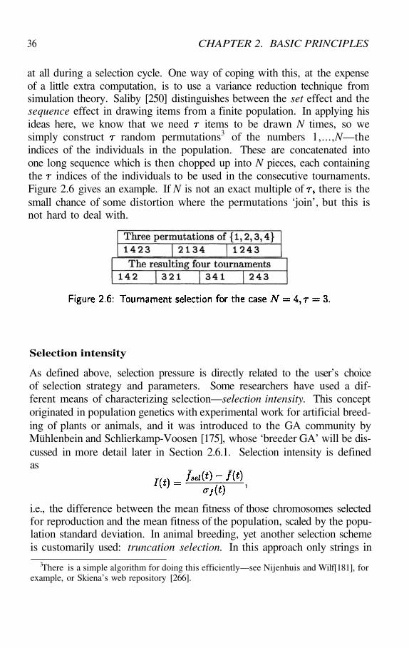
36 CHAPTER 2. BASIC PRINCIPLES
at all during a selection cycle. One way of coping with this, at the expenseof a little extra computation, is to use a variance reduction technique fromsimulation theory. Saliby [250] distinguishes between the set effect and thesequence effect in drawing items from a finite population. In applying hisideas here, we know that we need items to be drawn N times, so wesimply construct random permutations3 of the numbers 1,...,N—theindices of the individuals in the population. These are concatenated intoone long sequence which is then chopped up into N pieces, each containingthe indices of the individuals to be used in the consecutive tournaments.Figure 2.6 gives an example. If N is not an exact multiple of there is thesmall chance of some distortion where the permutations ‘join’, but this isnot hard to deal with.
Selection intensity
As defined above, selection pressure is directly related to the user’s choiceof selection strategy and parameters. Some researchers have used a dif-ferent means of characterizing selection—selection intensity. This conceptoriginated in population genetics with experimental work for artificial breed-ing of plants or animals, and it was introduced to the GA community byMühlenbein and Schlierkamp-Voosen [175], whose ‘breeder GA’ will be dis-cussed in more detail later in Section 2.6.1. Selection intensity is definedas
i.e., the difference between the mean fitness of those chromosomes selectedfor reproduction and the mean fitness of the population, scaled by the popu-lation standard deviation. In animal breeding, yet another selection schemeis customarily used: truncation selection. In this approach only strings in
3There is a simple algorithm for doing this efficiently—see Nijenhuis and Wilf[181], forexample, or Skiena’s web repository [266].

2.3. THE ELEMENTS OF A GENETIC ALGORITHM 37
the top P% of the population are eligible to reproduce; within this groupparents are chosen uniformly at random.
Selection intensity is clearly an a posteriori measure, and one that is alsospecific to the current population; if we make some assumption about thepopulation fitness distribution (commonly, that the distribution is stationaryand Normal), the value becomes a constant I(t) = I. Nevertheless, thevalue of I will still depend on the control parameters used for selection in anon-trivial way. While it is conceptually a more useful basis for comparingdifferent GAs, it is much more difficult to estimate than the simple selectionpressure. Further, it really only applies to strictly generational GAs and notto the élitist and steady-state versions, which will be described shortly inSection 2.3.7.
Blickle and Thiele [24] have surveyed several popular GA selection schemesand compared their theoretical values of I for a Normal fitness distribution.Their results enable the calculation of selection intensities from the controlparameters for these selection schemes, and thus to determine parametersettings for different schemes that give the same (expected) selection inten-sities. They also calculated some ‘second-order’ properties involving mea-sures of the ‘selection variance’ and ‘loss of diversity’. A notable result wasthat truncation selection involves a higher loss of diversity than any othermethod tested. Thierens [278] has recently extended this work to the caseof non-generational GAs.
Takeover time
Another measure sometimes used to compare selection schemes is the takeovertime. This computes the time taken for the best string to take over thewhole population, assuming only selection and no crossover or mutation. Itdepends on the population size as well as the parameters used for imple-menting selection. Hancock’s experimental work [112], referred to above,concentrated on takeover time as a measure.
Theoretical results can also be obtained. Goldberg and Deb [100] makesome simplifying assumptions for several selection strategies in order to ob-tain takeover time curves, which they found usually agreed well with ex-perimentally determined values. Their main finding was that takeover timetended to grow as for most strategies except fitness-proportionalselection, whose growth curve was They also gave a comparisonof time complexity, which showed that SUS and tournament selection arethe cheapest in terms of computational requirements. Rudolph [248, 249]has analysed a variety of more complicated selection schemes, all of which

38 CHAPTER 2. BASIC PRINCIPLES
turn out to have an growth for takeover times.
2.3.5 Crossover
Having selected parents in some way, we need to recombine them—the pro-cess called crossover. Crossover is simply a matter of replacing some ofthe alleles in one parent by alleles of the corresponding genes of the other.Suppose that we have 2 strings a and b, each consisting of 7 variables, i.e.
which represent two possible solutions to a problem. To implement one-pointcrossover a crossover point is chosen at random from thenumbers 1,..., 6, and a new solution produced by combining the pieces ofthe original ‘parents’. For instance, if the crossover point was 2, then the‘offspring’solutions would be
A similar prescription can be given for -point crossover where > 1.An early and thorough investigation of multi-point crossovers is that by
Eshelman et al. [72], who examined the biasing effect of traditional one-pointcrossover, and considered a range of alternatives. Their central argument isthat two sources of bias exist to be exploited in a genetic algorithm: posi-tional bias, and distributional bias. Simple crossover has considerablepositional bias, in that it favours substrings of contiguous bits, and we can-not be sure that this bias is working in favour of good solutions.
On the other hand, simple crossover has no distributional bias, in thatthe crossover point is chosen randomly using the uniform distribution. Butthis lack of bias is not necessarily a good thing either, as it limits theexchange of information between the parents. In [72], the possibilities ofchanging these biases, in particular by using multi-point crossover, wereinvestigated and empirical evidence strongly supported the suspicion thatone-point crossover is not the best option. Although the evidence was some-what ambiguous, it seemed to point to an 8-point crossover operator as thebest overall, in terms of the number of function evaluations needed to reachthe global optimum.
Another obvious alternative, which removes any bias, is to make thecrossover process completely random—the so-called uniform crossover. Thiscan be seen most easily by observing that the crossover operator itself canbe written as a binary string or mask—in fact, when implementing any
and
and

2.3. THE ELEMENTS OF A GENETIC ALGORITHM 39
crossover in a computer algorithm, this is the obvious way to do it. Anylinear crossover operator can be represented by a vector sothat the offspring of parents a and b is
where is the complement of and denote component-wise additionand multiplication respectively. For example, the mask
represents a 2-point crossover the offspring of a and b (as definedpreviously) being the vector (Another offspring canbe obtained by switching the rôles of a and b or, alternatively, by switchingthe roles of and ) By generating the pattern of 0s and 1s stochastically(using a Bernoulli distribution) we get uniform crossover which mightgenerate a mask such as
This idea was first used by Syswerda [277], who implicitly assumed that theBernoulli parameter Of course, this is not necessary: we can bias
towards one or other of the parents by choosing appropriately.De Jong and Spears [57] produced a theoretical analysis that was able
to characterize the amount of disruption introduced by a given crossoveroperator exactly. In particular, the amount of disruption in can betuned by choosing different values of .
Non-linear crossover
Treating crossover as a linear operator makes sense when dealing with binarystrings. However, when the representation is non-linear, crossover has to bereinterpreted. One of the most frequently occurring problems is where thesolution space is the space of permutations examples ofthis include many scheduling problems, and the famous travelling salesmanproblem (TSP).
For instance, the simple-minded application of in the following caseproduces an infeasible solution:

40 CHAPTER 2. BASIC PRINCIPLES
If this represents a TSP, the first offspring visits cities and twice, andnever reaches cities or at all, these problems being mirrored in the secondoffspring’s tour. A moment’s thought is enough to realize that this type ofbehaviour will be the rule, not an exception. Clearly we need to think ofsomething rather smarter if we are to be able to solve such problems.
One of the first ideas for such problems was the (partially matchedcrossover) operator [94]. Two crossover points are chosen uniformly at ran-dom between 1 and The section between these points defines aninterchange mapping. Thus might proceed as follows:
Here the segment between the crossover points defines an interchange map-ping
on their respective strings, which means that the cut blocks have beenswapped and now appear in different contexts from before. Another possi-bility is to apply a binary mask, as in linear crossover, but with a differentmeaning. Such a mask, generated as with say, might be the following
which is applied to the parents in turn. First the components correspondingto are copied from one parent, and then those that correspond to aretaken in the order they appear from the second parent in order to fill thegaps. Thus the above example generates the following pairs of strings:
This is one version of what is sometimes called order crossover, but it by nomeans exhausts the possibilities for dealing with permutations. A compre-hensive discussion of possible methods of attack is contained in papers byPox and McMahon [85] and Poon and Carter [190]. Furthermore, particularproblems raise particular issues. In the case of the TSP, for example, thepositions of the cities in the string is less important than their adjacencies,as has long been realized in OR when implementing local search methods forthe TSP. Recognising this, Whitley et al. [304] proposed the edge recombi-nation crossover for the TSP. Recombination becomes a matter of selecting

2.3. THE ELEMENTS OF A GENETIC ALGORITHM 41
edges from the combined edge sets of the two parents, rather than select-ing city positions from two permutations. More recent work by Nagataand Kobayashi [177] has also concentrated on edges—their edge assemblycrossover was the first case where GAs reliably found optimal solutions forlarge (> 3000 cities) TSPs.
Generalized point crossover
In fact, the TSP is only one of a substantial class of problems for which subsetselection is the key rather than linear combinations of strings. Radcliffe hasanalysed such problems very thoroughly in a series of papers [198, 199, 200,202], and the book by Falkenauer [76] also covers some examples of thistype.
The problem of needing different forms of crossover for different repre-sentations led Radcliffe and Surry [204] to propose a generalized form ofcrossover suitable for any representation. It is best described by thetemplate in Figure 2.7.
For the example above, suppose = 2, with crosspoints at loci 2 and 5,and the segment order is

42 CHAPTER 2. BASIC PRINCIPLES
The designated parent for the assignment of the first segment (segment 1)is P1, which gives
for the second (segment 3) it is P2, giving
and for the last segment (segment 2) it is P1 again, so we obtain
Finally, allele is the only legal assignment possible, so the offspring is
The definition of ‘compatible’ or ‘legal’ alleles may still be problem-specific,so this may appear over-complicated and unnecessary, and of course, stan-dard versions of crossover emerge as special cases. However, the advantageis that the same framework will apply should the alleles be edges insteadof cities. Using this edge set representation means we merely have two setsof edges, which could be placed in any order at all. However, for clarityof comparison we will maintain the order used above for the ‘allele=city’representation.
Using with the same parameters (and assuming symmetry so that, forexample, and are the same), the first two offspring steps are asfollows:
At the third step, only the edge in P1 is valid—clearly the edges and cannot be used again as they would create loops. In fact the onlylegal alleles left in either parent are and , so the final steps produce
In permutation representation this gives
and

2.3. THE ELEMENTS OF A GENETIC ALGORITHM 43
which is different from that produced using with the direct permutationrepresentation. (In fact, it is also a clone of the first parent, which may ormay not be a good thing!)
Thus, has the merit of constructing a general framework for recom-bination rather than relying on completely ad hoc ideas. A second offspringcan be generated by reversing the parental order, and can also easilybe generalized further to the case of more than 2 parents. Readers familiarwith Glover’s idea of scatter search [92] will also find some resonance here.
Inversion
Holland’s original presentation [124] included an operator that he calledinversion. The purpose of inversion was not to introduce new material,as with mutation, or recombine different genetic material, as in crossover.Rather it was a re-ordering, applied to an individual string, with the intent ofaltering the proximity of different genes prior to crossover. In order to makethis possible, the locus of each gene must be explicitly encoded along withthe allele at that locus. This means that there are many ways of encodinga particular string. For example, the following two strings are the same,where the first row denotes the locus and the second the allele:
However, when crossover is applied to the second string, the group of1s in the middle is less likely to be broken up than they are in the first.There is an obvious difficulty, however: what happens if the order of thetwo chromosomes selected for crossover is different? To deal with this, thechromosomes have to be aligned so that the order is the same in each case.This idea and its purpose is linked strongly to Holland’s idea of a schema,as will be seen in the next chapter.
Implementation issues
Of course, there are also many other practical considerations that influencethe implementation of crossover. How often do we apply it? Some practi-tioners always apply crossover, some never do, while others use a stochasticapproach, applying crossover with a probability Do we generate oneoffspring or two? In many cases natural offspring ‘twins’ will be created,although in more sophisticated problems it may be that only one offspringarises. If we choose only one from two, how do we do it? In accordance with

44 CHAPTER 2. BASIC PRINCIPLES
the stochastic nature of the GA, we may well decide to choose either of theoffspring at random. Alternatively, we could bias the decision by making useof some other property such as the relative fitness of the new individuals,or the loss (or gain) in diversity that results from choosing one rather thanthe other.
2.3.6 Mutation
First we note that in the case when crossover-OR-mutation is used, we mustfirst decide whether any mutation is carried out at all. Assuming that it is,the concept of mutation is even simpler than crossover: a gene (or subset ofgenes) is chosen randomly and the allele value of the chosen genes is changed.Again, this can easily be represented as a bit-string, so we generate a masksuch as
using a Bernoulli distribution—i.e., at each locus there is a small probabilityµ of a mutation occurring (indicated in the mask by a ). The above examplewould thus imply that the 2nd and 6th genes are assigned new allele values.However, it appears that there are variant ways of implementing this simpleidea that can make a substantial difference to the performance of a GA. Thecommonest idea seems to be to draw a random number for every gene in thestring, but this is clearly potentially expensive in terms of computation ifthe strings are long and the population is large. An efficient alternative is todraw a random variate from a Poisson distribution with parameter where
is the average number of mutations per chromosome. A common valuefor is 1—in other words, if is the string length, the mutation rate pergene is Having decided that there are (say) mutations, we draw
random numbers (without replacement) uniformly distributed between 1and in order to specify the loci where mutation is to take place.
In the case of binary strings, mutation simply means complementing thechosen bit(s). For example, the string
with mutation applied at genes 2 and 6, becomes
Mutation needs more careful consideration in the case of a q-ary coding.Since there are several possible allele values for each gene, mutation is no

2.3. THE ELEMENTS OF A GENETIC ALGORITHM 45
longer a simple matter; if we decide to change a particular allele, we mustprovide some means of deciding what its new value should be. This couldbe a stochastic choice, but if there is some ordinal relation between allelevalues, it may be more sensible to restrict the choice to alleles that are closeto the current value, or at least to bias the probability distribution in theirfavour.
It is often suggested that mutation has a somewhat secondary function,that of helping to preserve a reasonable level of population diversity—aninsurance policy which enables the process to escape from sub-optimal re-gions of the solution space, but not all authors agree. The balance betweencrossover and mutation is often a problem-specific one, and definite guide-lines are hard to give.
Several authors have suggested some type of adaptive mutation: for ex-ample, Fogarty [77] experimented with different mutation rates at differentloci. Reeves [216] varied the mutation probability according to the diver-sity in the population (measured in terms of the coefficient of variation offitnesses). More sophisticated procedures are possible, and anecdotal evi-dence suggests that many authors use varying mutation rates as a diversitymaintenance policy.
2.3.7 New population
Holland’s original GA assumed a generational replacement strategy: selec-tion, recombination and mutation were applied to a population of N chro-mosomes until a new set of N individuals had been generated. This set thenbecame the new population. From an optimization viewpoint this seems anodd thing to do—we may have spent considerable effort obtaining a goodsolution, only to run the risk of throwing it away and thus preventing itfrom taking part in further reproduction. For this reason, De Jong [55]introduced the concepts of élitism and population overlaps. The ideas aresimple—an élitist strategy ensures the survival of the best individual so farby preserving it and replacing only the remaining (N – 1) members of thepopulation with new strings. Overlapping populations take this a stage fur-ther by replacing only a fraction G (the generation gap) of the populationat each generation. Finally, taking this to its logical conclusion producesthe so-called steady-state or incremental strategies, in which only one newchromosome (or sometimes a pair) is generated at each stage. Davis [47]gives a good general introduction to this type of GA.
Slightly different strategies are commonly used in the ES community,which traditionally designates them either (Note that

46 CHAPTER 2. BASIC PRINCIPLES
these and µ, have a different meaning from those associated with mutationin the previous section.) In the first case, offspring are generated from
parents, and the best offspring are chosen to start the next generation4.For the + strategy, µ offspring are generated and the best individuals arechosen from the combined set of parents and offspring.
In the case of incremental reproduction it is also necessary to select mem-bers of the population for deletion. Some GAs have assumed that parentsare replaced by their children. Many implementations, such as Whitley’sGENITOR [301], use the tactic of deleting the worst member(s) of thepopulation, although (as Goldberg and Deb [100] have pointed out) thisexerts a very strong selective pressure on the search, which may need fairlylarge populations and high mutation rates to prevent a rapid loss of diver-sity. A milder prescription is to select from the worst P% of the population(for example, Reeves [216] used P = 50, i.e., selection from those worse thanthe median). This is easily implemented when rank-based selection is used.Yet another approach is to base deletion on the age of the strings.
Crowding and niching
Another aspect of the generation of a new population is the place of diver-sity maintenance. This has been a second-order consideration in many ofthe choices discussed above. It is also possible to make this a first-orderquestion, as with the concepts of crowding and niching. The terms againcome from a biological analogy: a niche in the natural environment is a setof conditions to which a specific group of phenotypes (a species, we mightsay) is particularly well adapted. In the GA, a niche is treated as a subsetof chromosomes that are in some sense similar.
The idea here is that a newly generated chromosome should replace onein its own niche, rather than potentially any one in the population. (Thisclearly relates only to overlapping populations.) De Jong [55] developed a‘crowding factor’ for use in such cases. This was an integer defining thesize of a (randomly chosen) subset of the existing population, with whichthe newly generated chromosome was compared. The one to which it wasclosest was the one to be deleted.
Other forms of niche generation have been proposed, of which the mostwell-known is sharing. This was first proposed by Goldberg and Richardson[95] who defined a sharing function over the population which is then usedto modify the fitness of each chromosome. The function could take many
4The strategy is also equivalent to truncation selection as defined earlier with[11].

2.3. THE ELEMENTS OF A GENETIC ALGORITHM 47
forms, but a simple linear function
was effective. Here is the distance between chromosomes and and Dis a parameter. The idea is that the sharing function is evaluated for eachpair of chromosomes in the population, and then the sum
is computed for each chromosome Finally the fitness of chromosome isadjusted by dividing the raw fitness values by the adjusted fitness valuesare then used in place of the original values. The purpose of this is thatchromosomes that occur in clusters should have their fitness devalued rela-tive to those which are fairly isolated. The only question is how to measuredistance. The obvious measure on the chromosomes is Hamming distance(especially for binary strings). As Hamming distance is so frequently used,we define it formally here:
Definition 2.2 The Hamming distance between two vectors and isgiven by
(This is also a good point to explain the square bracket notation [expr],originally introduced by Kenneth Iverson. When square brackets enclose alogical expression expr, they denote an indicator function, which takes thevalue 1 if expr is true and 0 otherwise. We shall make extensive use of thisnotation.)
Hamming distance is particularly useful in the case of binary strings, al-though (as the above definition makes clear) it is not restricted to this case.5
In the context of niching, however, and as alluded to above in Section 2.2.4,integers that are actually close can be mapped to binary representationsthat are far apart in Hamming space and vice-versa. While this is not aproblem with all representations, it may be preferable to define distances interms of the phenotype rather than the genotype.
5Hamming distance is frequently used in the analysis of RNA sequences, for example,where the underlying alphabet has cardinality 4.

48 CHAPTER 2. BASIC PRINCIPLES
Many other variations on the theme of niching have been proposed; arecent reference that provides comprehensive details is Horn and Goldberg[131].
2.3.8 Diversity maintenance
No less than John Holland himself has said that ‘the very essence of goodGA design is retention of diversity’ [127]. The effect of selection is to reducediversity, and some methods can reduce diversity very rapidly. This can bemitigated by having larger populations, or by having greater mutation rates,or by niching or crowding, all of which have some ‘natural’ basis for the waythey are performed. Later, in Section 2.6.2 we shall describe Eshelman’sidea of ‘incest prevention’. However, we need not be restricted to lookingfor phenomena that we see occurring in nature.
A popular approach, commonly linked with steady-state or incrementalGAs, is to use a ‘no duplicates’ policy [47]. This means that the offspringare not allowed into the population if they are merely clones of existingindividuals. The downside, of course, is the need to compare each currentindividual with the new candidate, which adds to the computational effortneeded—an important consideration with large populations. (In principle,some sort of ‘hashing’ approach could be used to speed this process up, butwhether this was used in [47] is not clear.)
We could also take steps to reduce the chance of cloning before offspringare generated. For instance on the two binary strings
cannot help but generate clones if the crossover point is any of the first threepositions. Booker [26] suggested that before applying crossover, we shouldexamine the selected parents to find suitable crosspoints—the ‘reduced sur-rogate’. A simple way of doing this entails computing an‘exclusive-OR’(XOR) between the parents, so that only positions between the outermost1s of the XOR string should be considered as crossover points. In the ex-ample above, the XOR string is
so that, as previously stated, only the last 3 crossover points will give rise toa different string. More generally, whenever there is one or more betweena pair of , the same offspring will result from the related crosspoints.In the above example, choosing the 4th or 5th crosspoint gives the sameoffspring.

2.4. ILLUSTRATIVE EXAMPLE 49
2.4 Illustrative Example
It is high time to provide a worked example of the implementation of a GA.As GAs are stochastic in nature, the first thing we need is a random numbersource. Most computer systems have built-in functions, and that isthe usual method of generating random numbers. The table below providessome random numbers that we shall use in what follows.
Suppose we wish to find the optimum of the cubic function defined inExample 2.4 above. Let us assume we have an initial population of size5. If we generate a random number then we assign each allele the value0 if and a 1 otherwise. Thus the first row in Table 2.1 generatesthe genotype string We can decode this to get the phenotype
and evaluate Following the sameprocedure with 4 more sets of random numbers produces the first generation:the initial population shown in Table 2.2. (Note that the random numbersinvolved have been omitted).
The final column in Table 2.2 is the fitness-proportional selection prob-ability, from which we can derive the following cumulative distribution forroulette-wheel selection:
Thus, returning to Table 2.1, our next random number is 0.185, whichimplies that we select string 1; the next is 0.367, which (as it lies between0.206 and 0.483) means that we select string 2. Now we perform crossoverand mutation on these strings. To apply one-point crossover, we have tochoose a crosspoint; this is selected with equal probability from the numbers1,2,3,4, using the following distribution:
As the next random number is 0.798, the chosen crosspoint is 4. If wecross the strings and at the 4th crosspoint, the resulting

50 CHAPTER 2. BASIC PRINCIPLES
strings are and again! This illustrates one of the prob-lems that we mentioned above—crossover can produce offspring that aremerely clones of their parents. (Section 2.3.8 discussed some consequencesof this, and how to prevent it.) For the moment, we shall choose one ofthese strings with equal probability: if the next random number is less than0.5, we choose the first, otherwise the second. As our next random numberfrom Table 2.1 is 0.236, we shall proceed with the first string, i.e.
Now we need to apply the mutation operator. We shall suppose thatthe mutation probability (or rate) µ in this case is 0.10 for each locus of thestring. Since the next random number is 0.174 (> 0.1), there is no changeto the allele value at locus 1. Similarly, the alleles at loci 2 and 3 remain thesame, but at locus 4, the random number is only 0.096, so the allele valuefor this gene changes from 1 to 0. There is no change at locus 5, so the finalstring is which decodes to with fitness
This procedure can then be repeated to produce a second generation, asseen in Table 2.3.
The search would continue by re-calculating the selection probabilities inorder to carry out a new cycle of selection, crossover and mutation. This isa very simple GA, but it has been effective in raising the population averagequite substantially, and it has actually found the optimum at step 2.

2.5. PRACTICAL CONSIDERATIONS 51
2.5 Practical Considerations
2.5.1 The importance of being random
GAs are highly stochastic algorithms, needing many random numbers, as canbe seen from the above example, and this has some important implications.One aspect of this has already been mentioned several times—the distortionthat can arise from using pure random sampling with replacement, and somemethods of variance reduction as used in the simulation literature have beenmentioned. Another important aspect, but one not widely publicised, is theneed to use a good pseudo-random number generator (PRNG). Ross [240]posted a message to the GA List Digest that contained a salutary lesson tothose who rely on the PRNGs provided with standard software. However,Meysenberg and Foster [165] conducted some extensive tests that failed toshow any systematic effect on GA performance due to different PRNGs, sothe case cited by Ross may be an isolated instance. Nonetheless, it is best tobe prepared, and the best advice is to use a PRNG that has been thoroughlytested, such as those described in the Numerical Recipes books [191].
2.5.2 Constrained optimization
So far we have ignored the question of constraints on the decision variablesof our problem, or implicitly assumed that the only constraints that matterare ‘box’ constraints on individual variables, which we may make use of inchoosing our representation, as in Section 2.2.4. However, in many casesthere may be quite complicated sets of constraints on the permissible values

52 CHAPTER 2. BASIC PRINCIPLES
of the phenotypic variables. The essence of the difficulty is clear: there israrely a guarantee (at least with simple operators and codings) that twofeasible parent solutions will provide feasible offspring. In some problemsit may even be difficult to find a reasonably diverse initial population offeasible solutions.
A popular strategy is to modify the fitness function by adding penaltyterms. Goldberg [96] gives the impression that this is a simple matter, andit is often worth trying it, but more extensive experience has suggested thatthis is seldom the best approach. We briefly discuss some of the alternativesbelow, but a far more detailed consideration of this question may be foundin the paper by Michalewicz and Schoenauer [167].
Penalties
The most obvious solution to the problem of constraints is simply to ignorethem. If an infeasible solution is encountered, it is not allowed to enter thepopulation (i.e., a ‘death penalty’). Unfortunately, this fails to recognizethat the degree of infeasibility does supply some information. It is commonto find the global optimum on or near a constraint boundary, so that solu-tions that are slightly infeasible may actually be fairly close to the optimum.(This is the argument made, for example, by proponents of the concept ofstrategic oscillation in tabu search [91].)
Thus, the obvious next step is to modify the objective function by in-corporating penalties. There are cases in which this works well, where the-oretical considerations permit an appropriate choice of penalty, but a naiveattempt to use penalties often fails. If the penalty is too small, many in-feasible solutions are allowed to propagate; if it is too large, the search isconfined to the interior of the search space, far from the boundaries of thefeasible region. Using variable penalties can be helpful [167].
Repair
Another popular solution to GAs for constrained problems is to accept aninfeasible solution, but to repair it before inserting it in the population.Some biological justification is often claimed for this approach, along thelines that the infeasible solution should be treated as an immature individualthat, although initially demonstrably unfit for its purpose, can neverthelessdevelop over time into a perfectly reasonable solution. This analogy has alsobeen applied to methods that use the GA offspring as the springboard fora local search. (Such hybrids have been given a more formal specification

2.5. PRACTICAL CONSIDERATIONS 53
under the name of memetic algorithms by Radcliffe and Surry [203].)In such cases, there is also the practical problem of deciding whether it
should be the original offspring or the repaired version that should be usedin the next generation. Inserting the repaired offspring means curtailing theexploration of a promising part of the search space. Davis and colleagues[48, 184] report some interesting experimental evidence, which suggests thatthe decision as to which to insert should be a stochastic one, with a fairlysmall probability of 5-10% of inserting the repaired version. There is also agood case for a mixture of approaches, where the original infeasible solutionenters the population, but it is given the repaired version’s fitness. Morewill be said about this idea below in Section 2.5.3.
Multiple objectives
Many authors have suggested using infeasibility as a secondary objective,thus avoiding the introduction of penalties. Recent work by Chu and Beasley[38] provides a good example of this idea in the context of set partitioning. Inaddition to the usual fitness measure (based on the true objective function),they define a secondary measure that they call unfitness to represent thedegree of infeasibility present in a given solution. The selection schemefor reproduction favoured strings that were maximally compatible, whileselection for deletion was carried out by trying to find an existing populationmember that was dominated by the new offspring—in the sense either thatits fitness is greater while its unfitness is no worse, or that its fitness isno worse while its unfitness is less. Multiple objective GAs (MOGAs) andtheir application have themselves been thoroughly reviewed by Fonseca andFleming [84].
Modified operators
One approach to alleviating the difficulties encountered by the standardoperators is to design operators that are appropriate for the problem. Theedge-recombination operator [304] for the TSP (Section 2.3.5) is a typicalexample.
Modified formulation
Another approach that has proved fruitful in some cases is to modify theproblem formulation. Reeves [219] found good solutions to bin-packing prob-lems by reformulating the problem. Rather than using the subset-selection

54 CHAPTER 2. BASIC PRINCIPLES
interpretation, bin packing was treated as a sequencing problem, with thesequence being decoded by using an on-line heuristic.
This type of problem re-formulation has also been used in other ap-plications. Schaffer and Eshelman [255] describe a similar approach to anextremely complicated line-balancing problem in the production of printedcircuit boards. The GA was used to find a good sequence to feed to a set ofheuristics that produced the final solution.
2.5.3 Hybridization
The effectiveness of a GA can nearly always be enhanced by hybridizationwith other heuristics. While one of the main benefits of using a GA is oftenprofessed to be its domain independence, this is also a common reason forGAs performing ineffectively. Introducing problem-specific knowledge canimprove solution quality considerably.
Hybridization can be carried out in various ways. The idea of seed-ing a population (as discussed above) with the results of applying anotherproblem-specific heuristic can be viewed as a type of hybridization, butthe most common approach is to integrate other heuristics such as neigh-bourhood search or simulated annealing into the normal GA cycle. Onceagain there are several different options, but a typical idea is to apply somestandard mutation and crossover operators to generate offspring, which arethen allowed to undergo further modification using NS before being insertedinto the next generation. How many of them undergo such improvement,whether the NS phase is carried on to a local optimum, whether steepestascent or something speedier is used, how population diversity is maintainedin the fact of fierce convergence pressure—these are examples of questionsthat have to be addressed in any particular implementation.
Lamarck or Baldwin?
Those who have some knowledge of the history of evolutionary theory willsee an obvious association of a typical hybridization scheme with Lamarck’sidea of the inheritance of acquired characteristics, but there is another ap-proach, associated with Baldwin [16]. An important early paper connectingthese ideas to GAs is that by Hinton and Nowlan [120]. In such cases, themodification is allowed to proceed in accordance with whatever rules havebeen decided. However, it is not the ‘mature’ individual that is insertedin the next generation, but the immature or original offspring from whichit was obtained. The essential characteristic of the ‘Baldwin effect’ is that

2.6. SPECIAL CASES 55
this immature individual then takes the fitness of its mature counterpart[308]. In a sense, the genotype is allowed to receive the credit for whatthe phenotype has ‘learned’ from its environment, so that genotypes thatpossess sufficient flexibility to permit learning will benefit relative to thosethat do not. Several comparisons have suggested that this is more effectivethan the Lamarckian approach; in particular, a complete issue of the journalEvolutionary Computation was devoted to this idea for the anniversary ofBaldwin’s original paper [281].
2.6 Special Cases
While this chapter has covered the basic principles of GAs, it should bevery clear by now that there are many ways of implementing a GA, andit is likely that—apart from those people who simply use one of the manypublicly-available codes, such as Goldberg’s simple GA [96]—everybody’sGA is unique! There are a few GAs that have a certain importance, eitherin the primacy of their ideas (such as GENITOR [301], which first system-atically advocated ranking), or in the rather particular way in which the GAis implemented. Three of these will be discussed in a little more detail, inorder to give a flavour of what is possible.
2.6.1 Breeder GA
Mühlenbein and Schlierkamp-Voosen [175] based their GA on the analogywe mentioned in Chapter 1—to artificial selection as performed by humanbreeders of plants and animals. A well tried and tested mixture of theoryand statistical experiments had been developed over the course of the lastcentury, dealing with concepts of selection intensity and heritability. Onthis foundation, the Breeder Genetic Algorithm (BGA) was constructed. Itis similar in spirit to the classical GA of Holland, but is applicable to contin-uous problems directly without the need for a discrete genotype. (Of course,the BGA can also be used for naturally discrete problems.) Mühlenbein andSchlierkamp-Voosen defined the BGA by means of 5 inter-related parame-ters:
String length
Initial frequency of desirable allele
Population size

56 CHAPTER 2. BASIC PRINCIPLES
Mutation rate
Selection intensity
The first two of these parameters are fixed by the representation, andby the initial population construction respectively. The other three are theones that really control the process. The notion of selection intensity hasbeen described above, and in this case, it relates to truncation selection6.The usual assumption is that phenotypic fitness is normally distributed, andfrom this I can be determined for different values of the truncation thresholdP.
Mutation in the BGA is carried out at a rate of 1/(string length)—a ratethat has often been claimed7 to be ‘optimal’: the sense in which it may beconsidered optimal is discussed in [175], where it is shown that there will alsobe an optimal population size for a given selection intensity and mutationrate. The fundamental idea here is that the requirements of recombinationand mutation are quite different. Mutation is more efficient in relativelysmall populations, while for recombination to work effectively the populationmust be large enough to possess sufficient numbers of advantageous allelesto try out in different combinations. These observations are not surprisingin themselves, but the quantitative analysis in [175] shows useful insights.In particular, these results appear to show that mutation has a rather moreinfluential rôle than it is sometimes accorded.
There is a caveat: the derivation of these results depend heavily onthe assumption that the fitness function is additive (and in many cases,are actually only derived for the Onemax function8)—i.e., precisely thosefunctions for which a GA is unlikely to be the best method to use! However,they are assumed to be valid guidelines for other more complicated functions,and for alternative forms of crossover and selection, and the experimentalevidence presented in [175] would appear to support this conclusion.
6A slightly different form of truncation selection is also sometimes used in breeding,where the best string takes place in all matings—an idea that Fairley [75] called HerdLeader breeding. This has recently been ‘re-discovered’ as the ‘stud’ GA [147]. Others(perhaps more politically correct) have preferred to call it ‘queen bee’ selection!
7Bremermann [30] was apparently the first to derive this result.8The Onemax function is defined in Appendix A.

2.6. SPECIAL CASES 57
2.6.2 CHC
Eshelman’s CHC9 algorithm [73] takes a quite different approach from theBGA. Here recombination is heavily emphasized, while mutation is usedpurely as a means to restart the algorithm when crossover’s progress hasmore or less ceased. The key principle for this version of a GA is the main-tenance of diversity. This is fostered by the use of a highly disruptive versionof (which Eshelman calls and by explicitly preventing ‘incest’—the mating of strings whose similarity is above some specified threshold. Toallow for the fact that populations cannot help but get more similar underthe influence of selection, this threshold is allowed to change as the numberof generations increases.
Selection is accomplished by what Eshelman calls a population élitiststrategy, which is essentially the strategy used by proponents of evolu-tion strategies, with the difference that (unlike ES) the number of offspringµ generated in CHC is variable. All members of the current populationare paired randomly, but not all are mated because of the requirement forincest prevention. Only the offspring of these matings are allowed to com-pete with the current population for survival. Thus, following each selec-tion/recombination step, the best of the strings are chosento form the next generation.
forces the exchange of exactly half of the non-matching bits (ornearly half, if this number is not an integer), so that the offspring areequidistant from their parents. To those who might object on the groundsof violating the ‘building block hypothesis’ (which we shall cover in somedepth in Chapter 3), Eshelman counters that such violations are relativelyinsignificant, and that the radical nature of the search accomplished by CHCis a worthwhile gain to put against this hypothetical loss.
Finally, without mutation, CHC is bound to converge to a point wherethe search stagnates unless the ban on incest is lifted completely. Eshelmantakes the view that this is the point at which mutation should be employed.The mutation rate (or divergence rate as Eshelman calls it) recommendedwould seem extraordinarily high (e.g., 0.35 per gene) in the context of ordi-nary GAs, but of course the purpose here is different. Furthermore, mutationis applied to one string only—the best one, and it is applied times.The new population thus consists of a single copy of the best string, togetherwith the mutated offspring.
With this new population a new recombination phase begins, with the
9According to Whitley [307], CHC stands for Cross-generational selection,Heterogeneous recombination and Cataclysmic mutation.

58 CHAPTER 2. BASIC PRINCIPLES
incest threshold reset to a value that depends on the mutation rate. In mostof the experiments on benchmark problem instances reported in [73], CHCwas run until a global optimum was found, but in general the process has noobvious stopping criterion. Thus some termination condition (e.g., a maxi-mum number of restarts, or a limit on the number of function evaluations)would have to be imposed externally. The results of the experiments cer-tainly demonstrated that CHC with a fixed population size of only 50 anda fixed divergence rate of 0.35 tends to outperform a traditional GA, evenwhen that GA’s parameter set is ‘optimal’, across a range of different typesof problem. Pseudocode for CHC is given in [73], and it is relatively easy toprogram it using this information.
2.6.3 GAVaPS
Population size has often been identified as a critical parameter in deter-mining whether or not a GA will work efficiently (or even at all). Withoutsufficient diversity, the search will get nowhere fast, but too large a popu-lation will slow it to a crawl and the available computational effort will beexhausted. CHC seems to provide a counter example, but only inasmuch asit approaches diversity maintenance in a different way. For standard GAs,the question of population size remains.
One interesting approach is that of Michalewicz, who allows the size ofthe population to vary by focusing on the age of a string. Age has beenmentioned before as a possible criterion for deletion in steady-state GAs,but in GAVaPS [166] the lifetime of a string is incorporated as an explicitparameter. Once the age of a string exceeds its lifetime, it is eliminated fromthe population. At each ‘generation’ a fixed proportion of the population isselected for recombination and crossover in the usual way, and the lifetimeof each offspring is set. This value is determined (within externally imposedlimits) by reference to population statistics: principally, the mean, minimumand maximum fitness of the current population; in some versions, the bestand worst fitnesses seen so far are also used.
Experimental evidence presented in [166] suggests that this approach,with minimum and maximum lifetimes set at 1 and 7 respectively, outper-forms a traditional GA with a fixed population. Actual population sizesshow an interesting profile: early in the search the population becomescomparatively large, but later it shrinks to a much smaller value. Similarbehaviour is also seen on a smaller scale whenever new high-fitness stringsare discovered. It is argued that this shows an efficient allocation of effort,allowing sufficient exploration to be balanced by effective exploitation. Of

2.7. SUMMARY 59
course, there is a potential drawback, in that at least two new parameters(minimum and maximum lifetimes) have to be specified, as well as the exis-tence of further scope for uncertainty as to what form the lifetime functionshould take.
2.7 Summary
This chapter has discussed the basic steps involved in implementing a ge-netic algorithm, and have outlined some special cases. It should by now beclear that GAs provide an unrivalled opportunity for variation in implemen-tation, each element having so many possible strategies, which in turn relyon so many quantitative parameters whose values can influence the GA’sperformance quite markedly. Three very different individual GAs have beendescribed to reinforce this point.
While this wealth of potential is part of the appeal of the GA paradigm,it is also somewhat frustrating, both for the practitioner and for the theorist.We hesitate to make a firm recommendation (someone will only disagree!),but would tentatively suggest that
An initial population of about 50 should contain sufficient alleles forthe GA to make useful progress.
Prior knowledge should be used along with randomization in choosingthe initial strings.
SUS and tournament selection are more efficient than the basic RWS.
Incremental reproduction and replacement usually make better use ofresources than the generational approach.
Two-point or uniform crossover have less positional bias than
An adaptive mutation rate appropriate to the application should beused, but if in doubt, a fixed rate of is a reasonable choice.
Diversity maintenance should be prominent in any implementation.
Hybridization should be used wherever possible; a GA is not a blackbox, but should use any problem-specific information available.
GAs are stochastic; there should be several replicate runs in any ap-plication.

60 CHAPTER 2. BASIC PRINCIPLES
From the practical side, some steps have been proposed to reduce thecomplexities of implementation. In the ES community, for instance, it hasbecome commonplace to make use of self-adaptive mutation rates (see [12,21] for a review of some of these developments). Recently Bäck et al. [14]have reported some experiments with a ‘parameter-less’ GA. Actually, asin the case of GAVaPS, with which it shares some similarities, parametershave not been eliminated—rather, they are replaced with different ones.However, it is hoped that the resulting algorithm might be less sensitivethan traditional GAs.
From the theoretical side, it would appear that probing more deeply intoquestions of how and why GAs work is vastly complicated by the existence ofsuch a diversity of approaches. However, the basic ideas of population-basedselection, recombination and mutation are common to everything that canbe called a GA. In the second part of this book we shall consider some of thetheoretical perspectives that have been applied, and we shall find that mostlythey deal with general principles of search strategy using recombination andmutation without being overly concerned with the details. We begin in thenext chapter by considering Holland’s original arguments, which make useof the key ideas of schemata.
2.8 Bibliographic Notes
Again, John Holland’s seminal work [124, 126] is well worth reading for aninsight into the development of the basic notions of a GA. David Goldberg’sbook [96] is deservedly well known for its clarity and careful organisation.Darrell Whitley’s tutorial paper [307] is an excellent summary of the basicprinciples of a GA, while other worthwhile sources of information are thebooks by Thomas Back [12] and Melanie Mitchell [170].
More idiosyncratic but nonetheless useful and interesting works are thoseby Michalewicz [166] and Falkenauer [76]. Ken De Jong’s thesis [55], whichdid so much to stimulate later enhancements of GAs is unfortunately un-published10, but he has recently produced a book [60] on evolutionary com-putation.
Genetic algorithms have developed as a subject of research in large mea-sure because of a few series of major conferences. At first, these were bi-ennial, with two series alternating between the USA and Europe. As thefield developed, other conferences began, and there are now many confer-
10However, scanned PDF files can be downloaded from George Mason University—seethe URL given in the bibliography.

2.8. BIBLIOGRAPHIC NOTES 61
ences each year in most parts of the world. The details of the proceedings ofmost of these conferences are listed in the bibliography (items [321]-[350]);readers interested in theoretical aspects of GAs will find that the biennialworkshops under the title Foundations of Genetic Algorithms (items [345]-[350]) contain much to supplement the relevant subject matter of the next6 chapters of this book.

62 CHAPTER 2. BASIC PRINCIPLES
Exercises
1.
2.
3.
4.
5.
A real-valued problem is to be solved by using a binary coding of thevariables. There are 6 variables; is known to lie in the interval[0,100], the rest are thought to be somewhere between –1000 and1000. The required precision is in the cases of and and
for the rest. Construct a suitable genotype-phenotype mapping.How long is the binary string? What is the binary representation ofthe point (20, –570, 120, –33, 33, 33)?
6.
7.
Prove the result
for the minimal population size, where the parameters have the mean-ing defined in Section 2.3.1.
Determine the values a, b necessary for linear scaling as defined inSection 2.3.4 with selection pressure
Prove the formulae stated in Section 2.3.4 for linear ranking:
and
(continuation) Verify that
where is a random number.
If strings are ranked in ascending order of fitness, show that the prob-ability of selecting the ranked string in soft tournament selectionwith is
where is the probability of choosing the better string in the tourna-ment, and hence prove its equivalence to linear ranking.
Geometric ranking (sometimes called exponential ranking) assumesthat the probability of selecting the ranked individual (in ascend-ing fitness order) is

2.8. BIBLIOGRAPHIC NOTES 63
Deduce suitable values of and assuming a selection pressure andevaluate them for the case N = 5, Compare the probabilitiesto those obtained for linear ranking with the same parameters.
8. Show that in tournament selection with the probability of se-lecting the ranked string is
By comparing the probability with that found in Exercise 7,deduce that this is approximately the same as geometric ranking if
9. Generate and compare examples of uniform (binary mask) order crossover,edge-recombination and GNX in both vertex and edge form for the fol-lowing TSP permutations:

This page intentionally left blank

Chapter 3
Schema Theory
Holland’s original insights into the analysis of GA behaviour have come infor some criticism over the years, but some of the basic ideas have provedfruitful, and it is entirely appropriate to review them at this point. As wehave already hinted, both he and Goldberg have argued strongly for theuse of binary encoding: in the terminology of Chapter 2—for the use of thesearch space (or a subset of it), rather than itself. His explanationfor this hinges on 3 main ideas, which we shall discuss at length in thischapter.
3.1 Schemata
However, prior to such a discussion we need to introduce his central conceptof a schema1.
Definition 3.1 A schema is a subset of the space in which all the stringsshare a particular set of defined values.
This can be represented by using the alphabet where the symbolis a ‘wild card’, i.e. it can be replaced by any of the possible alleles. In thebinary case for example, represents the subset of the 4-dimensionalhypercube in which both the first and last genes take the value 1,i.e., the strings
Schemata can thus be thought of in set-theoretic terms, as defining sub-sets of similar chromosomes, or geometrically, as defining hyperplanes in
1The word comes from the past tense of the Greek verb (echo, to have), whenceit came to mean shape or form; its plural is schemata.

66 CHAPTER 3. SCHEMA THEORY
space. Another interpretation is in terms of periodic ‘func-tions’ of different ‘frequencies’—for example, as illustrated in Figure 3.1 theschema represents the odd integers in the case where the chromo-some (genotype) encodes integer values (phenotype). As we shall see later,in the case of binary strings, these ‘functions’ have a particular form that isfundamental to much theoretical work.
It is clear that any specified chromosome is an instance of many schemata.In general, if the string has length each chromosome is an instance ofdistinct schemata, since at each locus it can take either a or its actualvalue. (We assume that the ‘degenerate’ cases—the string itself and theall string—are also schemata.) As a consequence of this, each time weevaluate the fitness of a given chromosome, we are gathering informationabout the average fitness of each of the schemata of which it is an instance.In the binary case, a population of size N could contain schemata, butof course in practice there will be considerable overlapping between stringsso that not all schemata will be equally represented, and some may have norepresentatives at all. (In fact we want them to have unequal representation,as the GA is suppose to focus attention on the ones that are fitter.)
3.1.1 Intrinsic or implicit parallelism
Holland claimed that in the sense that we are testing a large number ofpossibilities by means of a few trials, a GA possesses a property that heoriginally called intrinsic parallelism. Some other authors have used the al-ternative term implicit parallelism, and Holland himself later suggested [126]that this be adopted, reserving the term intrinsic to refer to the opportunityfor a software implementation of GAs in parallel.
The question is of course, how many schemata are being processed? To

3.1. SCHEMATA 67
answer this in general is a formidable task, but we can simplify by first
are respectively the distance between the first and last defined (i.e.positions on the schema, and the number of defined positions. Thus, theschema has length 3 and order 2.
The value can be thought of as a ‘transcription error’; it is of coursea function of schema fitness, length and order, as will be seen in the nextsection where we deal with the the Schema Theorem. For the moment, wewill assume that this restriction implies that we need only consider schemataof length say (where is a function of and of order
In order to estimate the number of schemata satisfying these conditions,we consider a ‘window’ of , contiguous loci counting from the leftmostposition. There are possible choices of defining loci for an orderschema in this window, each of which would give rise to actual schemata.(For example, where is a fixed value of or represents4 schemata corresponding to the 4 ways of choosing the fixed values.) Wenow successively move this window 1 step to the right, observing that eachtime there will be sets of defining loci that have not been counted inthe previous window. Altogether, we can move this window 1 step to theright times, so there are
possible schemata per string using Stirling’s approximationfor the factorials.
Of course, in a given string, all schemata are not represented for aparticular choice of defining loci, so lastly, we need to estimate how manyschemata meeting the prescribed conditions will occur in a population ofsize N. On the assumption that the members of the population are chosenusing uniform random sampling, a population of size (for a smallinteger value) would be expected to have instances of each of these order
schemata, so that with this definition of N, we can estimate the numberof schemata of length or less, and order as In fact, this isreally an under-estimate, since there are many other schemata we have notcounted at all, so this establishes a lower bound.
restricting the question to those schemata which have a probability ofsurviving.
We also need the notions of the length and order of a schema. These

68 CHAPTER 3. SCHEMA THEORY
3.2 The Schema Theorem
But how relevant is this idea of implicit parallelism? It is clearly impossibleto store the estimated average fitness values of all these schemata explicitly,nor is it obvious how to exploit such information even if we could. Thesecond plank of Holland’s argument was to show that by the application ofgenetic operators such as crossover and mutation, each schema representedin the current population will increase or decrease in line with its relativefitness, independently of what happens to other schemata.
In mathematical terms, he proved what has become known as the SchemaTheorem. We shall prove this theorem in the case of fitness-proportional se-lection. For this case, the fitness ratio is an importantparameter, expressing the average fitness of a schema relative to the averagefitness of the population. We have of course assumed here that the fitnessof a schema is the average fitness of all instances of that schema in thepopulation i.e.,
while
(Note that in general is a multiset, i.e., multiple occurrences of individ-ual chromosomes are possible—indeed, highly probable.) We approach thistheorem by proving the following results:
Lemma 3.1 Under a reproductive plan in which a parent is selected in pro-portion to its fitness, the expected number of instances of a schema S at time
is given by
where N(S,t) is the number of instances of S at time
Proof The result follows directly from the definition of fitness-proportionalselection.
Of course, this only describes what happens under selection. If crossoverand mutation are involved, instances of schema S may become instances ofsome other schema (destruction). At the same time, instances of other

3.2. THE SCHEMA THEOREM 69
schemata could recombine or mutate to become instances of S (construc-tion), but Holland chose to neglect them, so that he could state a resultabout S independently of all other schemata.
Lemma 3.2 If one-point crossover is applied at time with probability toa schema , S of length then the probability that S will be represented inthe population at time is bounded below by
where is the length of the chromosome, and is the probabilitythat the second parent is an instance of a different schema.
Proof The probability that schema S will be destroyed by the crossoveroperator is easily seen to be the product of the probability that crossover isapplied, and the probability that the crossover site lies within the lengthof the schema,
If the other parent is itself an instance of S, then S will survive regardlessof the crossover site; hence this must be multiplied by to give theprobability of destruction.
Hence the probability of non-destruction is
Finally, the probability of non-destruction is clearly only a lower boundon the probability of representation, since it is also possible for S to appearat time as a result of crossover of instances of two different schemata
and
For most selection and mating schemes, will depend only onS, so this is still independent of other members of the population. However,since the maximum value that can take is 1, the lower boundcould be replaced by
which removes any possibility that what happens to is dependent on therest of the population.
a schema S of order then the probability that S will be represented inthe population at time is bounded below by
Lemma 3.3 If mutation is applied at time with probability µ per gene to

70 CHAPTER 3. SCHEMA THEORY
Proof From the definition of mutation, the probability that mutation failsto destroy S is given by
Combining these results together we obtain the following theorem:
Theorem 3.4 (The Schema Theorem) Using a reproductive plan as de-fined above in which the probabilities of crossover and mutation are and µrespectively, and schema S of order length has fitness ratioat time then the expected number of representatives of schema S at time
is given by
Note 1 As noted above, the term can be ignored to leave theSchema Theorem in the form
which is a slightly simpler, and perhaps more commonly seen variation.
Note 2 The above statement of the theorem is still different from thatsometimes found. In particular, the left-hand-side is explicitly stated interms of expectation, a fact which is often insufficiently stressed; also theeffect of mutation is included. Secondly, the dynamic dependence of thefitnesses on the population is emphasized—again, something that not allstatements of the Schema Theorem make clear.
Note 3 While this development has assumed a generational GA with gene-wise mutation, one-point crossover and fitness-proportional selection, similarstatements can be found for other types of selection, crossover and mutation.A ‘generic’ version of the Schema Theorem would look like
where represents a ‘loss’ term relating to the ‘transcription error’ effectsof recombination and mutation, while is a ‘selection coefficient’. This

3.2. THE SCHEMA THEOREM 71
way of stating the Schema Theorem points up Holland’s basic idea thatthere are two competing forces in a GA—one increases the representationof good schemata in line with their fitness, while the other tends to breakthem up. So what characterizes the survivors?
3.2.1 Building block hypothesis
Consideration of the expression (3.2) shows that the representation of S inthe population is expected to increase provided that
Thus, short low-order schemata will increase their representation in the nextpopulation provided their fitness ratio is slightly more than 1; long and/orhigh-order schemata need much higher ratios.
The ideal situations for a GA would therefore seem to be those whereshort, low-order schemata or ‘building blocks’ are able to combine with eachother to form better solutions. The assumption that this is the GA’s modusoperandi is what Goldberg [96] calls the building block hypothesis. Thismight be a reasonable assumption in some problems, but how it can beensured in general is the real question—one we shall consider a little later.
3.2.2 The two-armed bandit analogy
Holland also attempted to model schema processing (or hyperplane compe-titions) by means of an analogy to a stochastic two-armed bandit problem.This is a well-known statistical problem: we are given two ‘levers’, whichif pulled give ‘payoff’ values according to different probability distributions.The problem is to use the results of previous pulls in order to maximize theoverall future expected payoff. In [124] it is argued that a GA approximatesan ‘optimal’ strategy, which allocates an exponentially increasing numberof trials to the observed better lever; this is then used to contend for thesupposed efficiency of a GA in distinguishing between competing schemataor hyperplanes.
Of course, this analogy assumes we might be solving problems of the form‘is better than In practice, we need to solve several ofthese problems (for example, ‘is also better than andunless they are independent, the sequence in which they are solved mightbe important. Further, we are usually interested in higher-order schemata.(If we are not, then the problem is by default a linear one, in which case

72 .3 SCHEMA THEORY
we should hardly be using a GA to solve it!) Thus there are really severalbandits, which have rather more than two arms. Nevertheless, Hollandargued that we can place a lower bound on the loss caused by making the‘wrong’ decision between several schemata, so that the theory could still beapplied.
3.2.3 Principle of minimal alphabets
Holland also used his schema-based theory to speculate on the ‘optimality’of binary encodings. The number of potential schemata is where
is the length of the string used to encode the decision variables, whichof course depends inversely on the cardinality of the alphabet Clearlythe exponent is more important than the factor and in fact, themaximum number of schemata will arise when is as large as possible, whichoccurs when the alphabet has as few symbols as possible, i.e., two. This hasbecome known as the ‘principle of minimal alphabets’ (PMA).
3.2.4 Does it work? Empirical evidence
We shall use the example of Section 2.4 again to illustrate what the under-lying schema averages may have to tell us. Table 3.1 contains the averagevalues for all the order-1 schemata given by the strings in the populationsrecorded in Tables 2.2 and 2.3.
This table reveals some interesting points for discussion. Firstly, the ‘pre-dictions’ of the order-1 schema averages (the lowest order building blocks) inthe initial population are almost all incorrect—the winners of the two-armedbandit competitions would suggest whereas the global optimum is
At the second stage, things are rather better, since the two-armedbandit would now suggest which has only one bit incorrect. Buthow did the GA manage to achieve this on the basis of schema theory, whenso many of the initial predictions were wrong? Secondly, the competitionsare not independent: consider the initial population schema averages for
and which actually comprise exactly the same subsetof
Of course, this example is open to criticism as being based on a verysimple problem, and using a very small population. However, as we shall see,it actually highlights quite neatly some of the problems of schema-processingarguments.
CHAPTER

3.2. THE SCHEMA THEOREM 73
3.2.5 Does it work? Analysis
We can treat some cases in greater analytical depth. For example, considera simple problem where strings have only two values:
Suppose we apply a simple GA to this function—fitness-proportional selec-tion, and bit-wise mutation at a rate µ . For convenience, within thissection we will denote the number of instances of S at generation asIt is easily seen that crossover has no effect in this case, so that the num-ber of instances of S in generation will be a binomial variable withparameters N (population size) and
The mean number of instances of S at the next generation is thus
More generally, we can define a Markov chain on the stateswith binomial transition probabilities. Chapter 5 will look at Markov chains

74 CHAPTER 3. SCHEMA THEORY
in some detail. For the moment, we merely note that the chain has theproperty that it is ergodic, since it is finite and all states communicate:the important thing about ergodicity for our purposes is that it means theprocess will have an equilibrium distribution. Without knowing a great dealabout Markov chains, we can find this distribution simply from the intuitiveidea that equilibrium will occur when the expected number of instances ofS remains the same in successive generations. This implies that for largeenough,
and the fraction will become a constant We thus obtain
Writing
reduces this to a quadratic
Ignoring terms of this gives
This is clearly less than 1—i.e., the equilibrium state does not consist ofstrings all of which are members of S. For example, with and
the equilibrium fraction of the population that belongs to S isonly 78%. If we assume that similar results apply to all order-1 schemata,and further, that these schemata are independent, it is clear that even formoderate values of string length the chance of the population containinga string that represents all hyperplane competition winners is quite small.Thus the schema-processing theory tends to suggest arguments why a GAshould not work efficiently!
3.3 Critiques of Schema-Based Theory
Our examples have suggested that all is not well with the ‘classical’ schematheory. Far from being special cases dreamt up to illustrate some unex-pected but unimportant quirks of the theory, these examples are actuallysymptomatic of a wider critical literature.

3.3. CRITIQUES OF SCHEMA-BASED THEORY 75
Schema theory has been critiqued from several directions. Firstly, asMühlenbein [173], has argued (echoing criticisms of the neo-Darwinian the-ory of evolution itself),
...the Schema Theorem is almost a tautology, only describingproportional selection...
Similarly, Holland records [127] that a criticism frequently levelled against itis that it is ‘either a tautology or incorrect’. This seems a little unfair: if thetheorem is incorrect, the mathematical errors should be pointed out—andnothing has appeared in the literature to challenge the mathematics. As forits being a tautology, there is of course a sense in which all mathematicaltheorems are tautologies—their conclusions are inherent in their premises,it is just that we did not originally discern them! Presumably, this criticismof the Schema Theorem supposes that the insights gained are so trivial asto be hardly worth the effort of pointing them out, but this is inevitably asubjective judgment.
However, Nick Radcliffe [198], Michael Vose [285] and others have raiseda much more serious challenge, by pointing out that the Theorem extendsto arbitrary subsets of the search space. In other words, there seems tobe no special ‘magic’ about Holland’s schemata. Vose [288] examined thefunction of mutation in a GA, and shown that a tiny change in the value ofthe mutation rate µ can cause a profound change in the GA’s trajectory—achange which no schema analysis can possibly predict. Vose [294] contendsfurther that the focus on the number of instances of a schema that surviveis misplaced. What is far more important is which instances of a schemaappear in the next population. The subset of strings represented by a schemausually has a fair amount of fitness variability (this is an aspect of epistasis),so the new set of strings in the next population is not necessarily as fit as theprevious one. (On the other hand, if the epistasis is low, there are almostcertainly simpler methods of finding the optimum anyway.)
All this is rather obscured by some statements of the Schema Theorem,including Holland’s and Goldberg’s, where the stochastic and dynamic na-ture of the quantities involved is brushed aside. In turn, this has led tothe implications of the theorem being pushed further than can be sustained.One of the most glaring problems arises from the much quoted concept of‘exponentially increasing’ trials of good schemata. It is worth rehearsingthis argument for a moment, in order to point out where it goes wrong.
By ignoring the fact that the RHS of Equation (3.2) is an expectation,an inequality of the form

76 CHAPTER 3. SCHEMA THEORY
can be set up for those schemata that are ‘consistently above average’,expressing the ‘excess fitness’ required in accordance with Equation (3.4).This is then iterated to suggest that the number of instances of S will growin accordance with a geometric progression (the discrete time analogy ofexponential growth, which is more properly related to continuous time).
Why is this false? Firstly, we have the fact that the true relationship isstochastic, so we should not really confuse the actual number of instancesof in the equation by its expected value, unless we have an infinite pop-ulation. But, more importantly, the ‘growth factor’ will not remain ata constant level. Putting it another way, no schema can stay ‘consistentlyabove average’; rather, its fitness will shrink towards the population average.For if S does find itself with increased representation in the next population,the ‘excess fitness’ will almost certainly be smaller, since the intersection ofS and is larger. Thus there will be a tendency for the schemaaverage to approach the population average, and at some point, because ofthe disruptive effects of crossover and mutation, the ‘excess’ will becomea deficit. An example of this process can be seen in the previous section,where the schema average for in Table 3.1 increased from 3455 to3587, yet its fitness ratio has shrunk from 1.49 to 1.29. Finally, it shouldbe unnecessary to point out that even if we had an exponential increase, itwould have to end quite soon when we have a finite population. The rate ofgrowth of a ‘good’ schema is much more likely to resemble a sigmoidal curvethan an exponential. Nor is there any guarantee that the final state willconsist of 100% representation of a given schema, as we saw in the exampleof Section 3.2.5 above.
In other words, Holland’s Schema Theorem is a neat device for expressingwhat happens (on the average) to a schema S as we pass from one generationto the next. It is true that it makes a statement about S that does not rely onknowledge of any other schema. However, unless we know what happens tothose other schemata as well, we cannot use it to extrapolate the trajectoryof S beyond that next generation.
The idea of implicit parallelism is also of strictly limited application.It merely describes the number of schemata that are likely to be presentgiven certain assumptions about string length, population size and (mostimportantly) the way in which the population has been generated—the lastassumption being one that is unlikely to be true except at a very earlystage of the search. Bertoni and Dorigo [19] have pointed out that Holland’s
lower bound relies upon a particular relationship between populationsize and m—the maximum schema order considered in the derivation, theassumption being that By considering the case for a

3.3. CRITIQUES OF SCHEMA-BASED THEORY 77
range of values of they extended the argument to deal with an arbitrarypopulation size, and show that the relationship can in fact be anything atall!
Moreover, the assumption that the population is independently and uni-formly distributed is still required, so the lower bound may be of little prac-tical relevance except in the case of the initial population. Finally, the ideathat all these schemata can then be usefully processed in parallel is falsefor another reason, which ties in to problems with the two-armed banditanalogy.
A problem with an inappropriate application of the central limit the-orem in Holland’s original proof was highlighted in the 2nd edition of hisbook [126], although the essential core of his two-armed bandit argumentwas untouched. However, Rudolph [246] has recently shown that the two-armed bandit argument breaks down in a much more fundamental way:Holland’s ‘optimal’ strategy for the bandit problem is comprehensively out-performed by an alternative approach that uses a sequential likelihood ratiotest. Macready and Wolpert [155], as well as pointing out a flaw in Holland’smathematics, have independently argued, using a Bayesian framework, thatthere is no reason to believe that Holland’s strategy is an optimal one. Itfollows that, even if we were to accept that the GA adopts a strategy of‘exponentially increasing trials’, it is in any case not the best way of solvinga competition between two competing schemata or hyperplanes.
Moreover, as mentioned in [218] (to be expanded upon later in Chap-ter 8), the assumption that hyperplane competitions can be isolated and‘solved’ independently is false, unless the population has a very particularcomposition. That is, the GA is not really solving, concurrently and inde-pendently, two-armed (let alone multi-armed) bandit problems, sincethe arms cannot be ‘moved’ independently. Again, this has been illustratedin the example of Section 3.2.4.
In general, it may be difficult even to identify the arms properly; asshown later (Chapter 8), we may think we are contrasting with
when the results we obtain are due to differences between (say)the schemata and an effect thatstatisticians are well acquainted with as ‘aliasing’ or ‘confounding’.
Some of the other principles erected on the foundations of schema the-ory have also inevitably faced criticism. The PMA has been questioned:Antonisse [9] pointed out that what is meant by a ‘schema’ for higher-cardinality alphabets is not necessarily the same as it is in the binary case,where each can only be replaced either by or With non-binary en-codings, he argued, we should consider all subsets that could replace a *,

78 CHAPTER 3. SCHEMA THEORY
counting each of them as a possible schema. From this perspective, there aremany more schemata available to higher-cardinality alphabets. Of coursethe question is whether it matters—is the potential number of schemata im-portant anyway, if they cannot be processed independently? On the otherside of the argument, some practical support for the PMA does come fromthe fact that it may allow the use of smaller populations, as discussed inChapter 2, and also from some experimental work by Rees and Koehler[212].
The BBH has also come in for some examination. Goldberg [97] in-troduced the idea of a ‘deceptive’ function—one which would lead the GAin the ‘wrong’ direction, since the ‘building blocks’ needed for a successfuloptimization were not present. As expected, GAs can find such problemsvery hard to solve [302], although the extent of the difficulty also dependson the amount of deception [107]. This is however mainly ‘negative’ evi-dence for the BBH; Mitchell et al. [169] described some experiences with theso-called ‘Royal Road’ function—a function that was meant to demonstratethe positive side of the BBH, in that it provided an environment for a GAto build an optimizing solution step by step, in the manner in which a GAwas thought to behave.2 It was somewhat disconcerting to find that the GAwas comprehensively outperformed by a simple hill-climber—on a functionthat should have been ideal for the supposed modus operandi of a geneticalgorithm.
However, that a GA really works like this is not likely anyway. Thornton[279] has pointed out that the requirements of the BBH are actually atvariance with those of the Schema Theorem. The latter favours short, low-order schemata—as the building blocks become longer or more specific (asthe BBH proposes) their representation in the next population is expectedto diminish rather than increase. So there are many reasons why schematheory does not deliver the explanation for GA behaviour that it originallyappeared to promise.
3.4 Surveying the Wreckage
In the late 1980s and early 1990s, schema theory and implicit parallelismseemed to provide a satisfying explanation for the utility of GAs, and evenin some quarters for claims that they were in some sense the ‘best’ algo-rithm possible. ‘Violations’ of schema theory were thought to be significant:consider the statement
2Royal Road functions are described in Appendix A.

3.4. SURVEYING THE WRECKAGE 79
The most serious objection to ranking is that it violates the schematheorem... [301]
where the objection was answered, not by a critical examination of theTheorem, but by re-interpreting the idea of fitness so that it could still beapplied.
It should be appreciated that Holland’s original account of the SchemaTheorem and its ramifications were always rather more nuanced than thatprovided by some of the later enthusiasts for GAs. His discussion of ‘expo-nential growth’ in the second edition of his book [126], for example, clearlyqualifies it as ‘until its instances constitute a significant fraction of the to-tal population’ (although he leaves unstated what we should understand by‘significant’). Furthermore, Holland’s emphasis was much less on findingoptimal solutions, which assume a ‘best-so-far’ criterion in evaluating theeffectiveness of a search, than it was on populations adapting to an envi-ronment, for which ‘online average fitness’ (the average of all individualsgenerated over the course of time) is arguably a more sensible measure ofeffectiveness. De Jong (who, ironically, did a great deal towards developingthe optimizing aspects of GAs) has cautioned in a number of papers [56, 58]that we should not treat Holland’s original vision of a GA (and its con-comitant ‘theory’) merely as a function optimizer—preferring the acronym‘GAFO’ for the application that has now become the most popular.
Nevertheless, the implications of these caveats have often been neglectedby later researchers, so it may seem somewhat disconcerting to find that, overthe course of the 1990s, Holland’s GA theory has been so comprehensivelyeviscerated. Vose, for example, has said that
...schema theory tells us almost nothing about GA behaviour...[293]
a judgment which clearly dismays John Holland [127]. It is not in any spiritof triumphalism that we have described the shortcomings of schema theory,nor would we wish to diminish the contribution of earlier researchers. Thisis the way science develops.
Neither is it to say that schemata must be completely consigned to thedustbin while we cast around for newer and better ways of describing theprocess of the genetic algorithm. The suggestion that schema theory tellsus ‘almost nothing’ might be considered excessive, although the theory isclearly a lot less useful than we once thought. The idea of a schema is still auseful one, if rather more limited than it at first appeared. The notion thatwe should look for and try to exploit structure in a fitness function is surely

80 CHAPTER 3. SCHEMA THEORY
sensible—although Holland’s schemata will not necessarily accomplish thatobjective. Radcliffe [198, 199] has argued that in implementing a GA, weneed to take account of the properties of the operators employed as well asthe way in which a solution is represented. This is clarified by the work ofAltenberg in putting the Schema Theorem into a wider context.
3.4.1 Price’s theorem
Altenberg’s work [5] related the Schema Theorem to earlier work in pop-ulation genetics. Price [192] had shown how the expected value of somepopulation trait could be related to the correlation of that trait with fitness.If we have some measurement function for the trait (where is astring in the current population), then Price’s theorem can be expressed asfollows:
to be the value of F averaged over all possible offspring of andThen the average value of F in the next generation is
where (resp. is the fitness ratio of string (resp. andand are respectively the mean of and its covariance with fitness,evaluated over all pairs in each case. [These quantities are all param-eterized by to emphasize that they are calculated with respect to the currentpopulation.]
This looks fairly complicated, but as Altenberg shows, it is a more generalformulation than the Schema Theorem. In particular, if the measurementfunction is given as
so that the trait of interest is membership of schema S, the Schema Theorememerges as a special case. With this definition of F, firstly we obtain
where is written in terms of S to emphasize that it now represents thoseoffspring of and which are members of schema S. Further, a lower boundon can easily be written for any S, if we know the operator (e.g., andthe schema theorem emerges in the form
Theorem 3.5 (Price) For any pair of parents at time define

3.4. SURVEYING THE WRECKAGE 81
It can thus be seen that for S to grow in frequency, there must be a pos-itive correlation between the fitness of a string, and its membership of S.However, whether fitness and schema membership are correlated will beproblem-dependent, and even when such a correlation exists it can only bemeasured with respect to the current population. Furthermore, while theSchema Theorem has very little to say about the operators—relegating themto transmission error status as in Equation (3.3)—Altenberg shows theirrelevance. For example, different recombination operators induce differentfitness distributions, and ‘progress’ will only be made where the correlationis in the right direction.
Other work has also suggested the importance of correlations: Mandericket al. [157], for example, proposed that local parent-offspring correlationsshould be monitored in order to verify that the GA makes progress. Whilethis idea is intuitively sensible, Altenberg produces two counter-examples toshow that such measures are not sufficient to predict GA performance.
3.4.2 Formae and respect
Altenberg’s is not the only work to point out the mistake of ignoring theconstructive effect of the operators. Whereas a schema defines subsets ofchromosomes that are similar in the specific sense that they have the samealleles at some stated loci, Radcliffe’s concept [198, 199, 200, 202, 204] ofa forma defines subsets of chromosomes that are similar in a more generalway—perhaps in terms of the phenotype rather than in terms only of thegenotype. For example, in the case of bin packing, the defining characteristicof a forma might be that a particular group of objects is packed together,while for the TSP, it might be that a chromosome possesses a particular edge.With Radcliffe’s approach, it is possible to design operators a priori to havedesirable properties in the context of the chosen means of representation.For example, he argues that it is often sensible to require operators to respectthe formae of which the parents are instances. This means that whereparents share a particular characteristic, their offspring should inherit thischaracteristic.
This aspect of commonality has been stressed several times; Reeves [214]pointed out the relevance of which string (out of all those in the common sub-set represented by the schema) is selected. Höhn and Reeves [121] suggestedthat the two-fold effect of crossover should be explicitly recognized—the firsteffect being the inheritance of common genetic material, the second beingto explore the consequently reduced search space by means of an operator.Superior results for graph partitioning were obtained when this approach

82 CHAPTER 3. SCHEMA THEORY
was used. This is also true for Falkenauer’s ‘grouping GA’ [76], which usesthe same idea, if not the same terminology. A ‘commonality-based’ SchemaTheorem has been provided more recently by Chen and Smith [37].
3.4.3 Modifications
The acknowledged inadequacies of the original Schema Theorem have alsostimulated new lines of enquiry. One is to take account of both ‘gains’ and‘losses’ in the process of recombination, so that the Schema Theorem canbe written as an equation, instead of a lower bound. The version in [37] isa recent attempt to deal with this question, but such ideas go back at leastto Bridges and Goldberg [31].
Anotherapproach has been taken by Stephens and Waelbroeck [272, 273]who construct an exact version of the Schema Theorem by recursively par-titioning schemata into ‘left’ and ‘right’ pairs of lower order and shorterlength than the original, until all schemata are of order 1. (The formulationis necessarily somewhat complicated, but it is closely related to that dueto Altenberg [5], discussed above as Theorem 3.5.) Their analysis is ableto demonstrate that the lower bound obtained from the traditional SchemaTheorem can sometimes be far from sharp: schemata that (using the tradi-tional approach) ought not to survive may in fact do so quite easily if thecurrent population is able to create more instances than are lost by meansof disruptive effects.
More recently Poli [188] extended this idea of recursively partitioningschemata in order to derive a probability distribution for the number ofinstances of a schema that survive. Poli points out that, given a transmission
for For example, if and we ignore mutation, the transmissionprobability for is found by considering S itself and its ‘compo-nents’ and
probability for schema S, the number of instances of S at is aBinomial variable with probability
and expectation
The Stephens-Waelbroeck theorem can then be recast as a recursive formula

3.4. SURVEYING THE WRECKAGE 83
The difficulty in extending this is firstly the large number of recursive termsthat are needed for high-order schemata, and secondly the complexities ofcalculating the required binomial probabilities. The latter problem Polideals with by using well-known statistical inequalities to obtain stochasticlower bounds. However, despite using bounds that are fairly weak, it stillinvolves a Herculean amount of labour in order to reach a statement ofpractical significance.
3.4.4 New test functions
Another viewpoint is that taken by John Holland himself [127]. He considersthat the problem with the building block theory is the stochastic effects of aGA that are neglected in his (and others') use of the Schema Theorem. Theoriginal Royal Road (RR) functions [169] failed to demonstrate the utility ofGAs for several reasons. As Watson et al. [298] have also pointed out, RRfunctions were too easy; this led in [298] to the development of ‘hierarchicalif-and-only-if’ (HIFF) functions,3 and in Holland's case [127] to 'hyperplane-defined functions' (HDFs), both of which are more challenging to searchalgorithms.
More fundamentally, RR functions highlighted a general problem inGAs—the phenomenon of ‘hitchhiking’. This occurs where a particularlow-order schema (perhaps just a single allele) has a significant influenceon fitness. As selection and reproduction spread instances of this schemathrough the population, it is probable that alleles present in the first exam-ples of the schema will hitch a ride, whether or not they are really importantor not. For example, if has a high relative fitness, and its firstoccurrence is as there is a high probability that the popula-tion will soon consist largely of instances not only of but alsoof This would not matter too much if reallyis important from a global perspective, but if (say) is evenbetter, the prevalence of may prevent the GA from finding it.Of course, this is just another aspect of the problem of loss of diversity thatwe discussed in Chapter 2. Higher mutation rates or lower selection pres-sure might counteract it, but the consequently greater stochastic variabilitymight prevent anything from becoming established at all.
3Further details of HIFF functions can be found in Appendix A.

84 CHAPTER 3. SCHEMA THEORY
This dilemma led Holland to propose ‘cohort GAs’ (cGAs) [127], whereinstead of the relative fitness of a string determining the number of offspringit can have, it determines the frequency with which the string is allowed toreproduce. This is accomplished by delaying reproduction by an amountthat depends on fitness. However, although Holland motivates the cGA byschema-processing arguments, it is not clear that such arguments amountto a sine qua non for this approach.
3.5 Exact Models
Perhaps the most satisfying and elegant development stemming from dissat-isfaction with schema-processing arguments is the formal executable modelproposed by Vose [287] and Whitley [306], building on an earlier suggestionby Vose and Liepins [286]. This places the focus on the strings rather thanon the schemata, although of course it is conceptually simple to move fromone to the other. The complete dynamical system model of which this is thebasis will be treated at length in Chapter 6, but it is appropriate to providea simple introduction at this point.
A model that takes account of construction of strings (or schemata) aswell as destruction needs to consider all possible ways of performing crossoverand mutation. In the most general case—uniform crossover on complemen-tary strings—every string in the Universe can potentially be constructed.This effect can be captured by a 3-dimensional array of probabilities, wherethe strings or vectors are indexed from 0 to The entry ofthis array gives the probability that vectors and will recombine to pro-duce vector The effect of mutation is similar to represent, but since onlyone string is involved, it is rather easier. Conceptually, this approach hasproved to be rather successful in providing insights into GAs, as Chapter 6will show.
However, for practical purposes, even a 10-bit chromosome would giverise to more than entries, placing extreme demands on computationalresources for applications of any reasonable size. Fortunately, as Vose andLiepins pointed out [286], a 2-dimensional matrix is sufficient to representthe effects of recombination. Assuming we have such a matrix for generatingone arbitrary vector (suppose, for convenience, it is the all-zeroes vector,denoted simply by a simple permutation mapping suffices to determinethe matrix for any other vector. Suppose we have the ‘mixing matrix’ withentries
and generate vector

3.5. EXACT MODELS 85
and we wish to generate the matrix for another vector this matrix is
where, as usual, is ‘exclusive OR’, or addition modulo 2. (Note that weregard as both indices and vectors for simplicity of notation.) Asfor the entries themselves, these are clearly operator-specific. For example,suppose we have with parameter probability of selecting fromvector the following is the mixing matrix for vectors of length 3, indexedin standard binary integer order.
To illustrate the permutation mapping, suppose we want the mixing prob-ability for vectors and to produce vectorThis probability is clearly since the second bit must come from andthe others from In terms of the mapping function, we need
and
and as expected. Whitley [306] gives an algorithm forgenerating the mixing matrix for some other operators in the case of binaryvectors, and Whitley and Yoo extend this to the case of permutationoperators such as Mutation can also be handled in a similar fashion.
Having obtained a mixing matrix M, the model determines the evolutionof the probability of vector in the population as
where the vector contains the probabilities of selection for all stringswhich implicitly includes the necessary fitness information. By use of thepermutation mapping, Equation (3.6) can then be extended to all strings.Chapter 6 will show how these ideas can be developed in much greater detail.

86 CHAPTER 3. SCHEMA THEORY
3.6 Walsh Transforms and deception
Another enduring legacy of the interest in schemata has been the applicationof Walsh transforms to binary GAs. Much of the analysis that we shalldescribe later in this book will require some understanding of Walsh analysis,and this seems an appropriate place to introduce the topic.
The idea of applying Walsh transforms in GAs was first developed byBethke [20], but it is David Goldberg [98, 99] who deserves much of thecredit for its wider recognition. The focus in these initial investigations wasstill on schemata: in particular, what sort of function it might be that could‘fool’ a GA—in the sense that the schema averages would point the GA inthe ‘wrong’ direction, away from the global optimum. Such a function isshown in Table 3.2. Note that definitions of this function in the literaturemay differ in unimportant details.
If we examine the schema averages here we find that while is theoptimalpoint, any schema that contains is less fit than the correspondingschema that contains : for example, Goldberg calledthis phenomenon deception. But how could such a function be constructed?This is where the Walsh transform is useful.
3.6.1 Function Decomposition
Suppose we have a function defined for a variable It is natural to askif this function can be decomposed into a superposition of simpler functions

3.6. WALSH TRANSFORMS AND DECEPTION 87
where the ideally should have some meaning that can be related to prop-erties of the function In the case of GAs, we normally have representedas a vector (often a binary string), which we shall denote by and its com-ponents by Occasionally it will be convenient to abuse our notation andwrite or as seems most appropriate. The most well-known set of func-tions for binary strings is the set of Walsh functions, which may be definedas follows:
where is the binary vector representing the integer (and represents itscomponents). There are several equivalent definitions: one such is
where is the bitwise operator, and is the parity function
For example, if and which means that we findthat with odd parity, so that
For strings of length there are Walsh functions, so that the full decom-position is
Such a decomposition is of course a close analogy of what is done for func-tions of real numbers. There it is known as a Fourier decomposition, andentails the superposition of trigonometric functions—of which Walsh func-tions are a discrete analogue, forming a set of rectangular waveforms. Forexample, the function is as shown in Figure 3.2.
The Walsh coefficients can be obtained from the values of bymeans of the Walsh transform
Note that this can also be expressed in a matrix form as

88 CHAPTER 3. SCHEMA THEORY
where the matrix has elements
and is an inner product. As in the case of Fourier trans-forms, there are computational algorithms that can speed up the process.One such is Yates’ algorithm [319] (see Exercise 6 at the end of this chapter),but a wealth of detail on such matters can be found in [17].4
All this is interesting, but what does it have to do with schemata? Read-ers may observe a strong similarity between Figures 3.2 and 3.1. This is nocoincidence. With the use of some simple algebra and arithmetic it can beshown that schema averages are easily computed from appropriate subsetsof the Walsh coefficients, and vice-versa. It can easily be seen that, forexample,
the mean of all fitnesses, while
with similar results for more specific schemata. Table 3.3 provides the co-efficients that result from such calculations for the deceptive function ofTable 3.2.
It is thus possible to work backwards from the deception conditionsetc., in order to obtain conditions on the Walsh coef-
ficients that will deliver us a deceptive function. This is in fact how Gold-berg’s function was originally determined. (Two of the constraints derivedin are, however, incorrect; more will be said on this point in Chapter 8).
4It should be noted that the Walsh literature has different notions of numbering theWalsh functions. That used in this book follows Goldberg [98, 99] rather than the standardorder used in [17].

3.6. WALSH TRANSFORMS AND DECEPTION 89
3.6.2 More on deception
Early theoretical work was still heavily influenced by schema theory, andtended to concentrate quite markedly on deception and its analysis. Whit-ley was able to characterize the degrees of deception in terms of differentorders of schema competition [302, 305], and he also defined what is meantby the concepts ‘fully’ and ‘consistently’ deceptive. For binary strings, healso showed that the deceptive attractor is the complement of the global op-timum, and although it is not necessarily a Hamming space local optimum,it must at least be a Hamming neighbour of such a local optimum. Thisis a convenient point to remark that discussion of what is a hard or easyproblem for a GA is often bedevilled by a lack of caution in transferringbetween those ideas of relevance specifically to neighbourhood search andthose relating to GAs. It cannot be assumed that what is a local optimumfor one representation or algorithm is necessarily so for another. We shallreturn to this question in Chapters 8 and 9, but this will serve as an earlywarning that such analyses may need to be fairly sophisticated.
Whitley also pointed out that in order to be deceptive, it was sufficientthat (assuming, without loss of generality, the global optimum to be theall- string) for any string with k is fitter than anystring with —a rather simpler means of construction than theWalsh-based approach. He also argued strongly that the only challengingproblems for a GA are deceptive. However, Grefenstette [107] later producedan example to show that deception does not necessarily make life hard fora GA:
Since the schema has a mean fitness only half that ofthis function certainly qualifies as deceptive. Nevertheless, as Grefenstettediscovered, most GAs will ‘solve’ this problem easily. The reason is thatonce an instance of is found (which is not unlikely, given a rea-sonable population size), this particular subset of will quickly

90 CHAPTER 3. SCHEMA THEORY
spread and other instances of the lower-order schema will disappear. Theproblem is deceptive from a global perspective, but in practice the GA willonly ‘see’ the local situation. Once again, Vose’s earlier point is relevant—itis the strings themselves that matter, not just the schemata. The stringsin the population at a given time may have schema averages that are quitedifferent from those that would be obtained from the Universe of all strings.However, while deception does not necessarily mean practical difficulty for aGA, it should not be assumed that its absence make life easy. The fact is thatany estimates of (true) average schema fitness could be wildly inaccurate—particularly for low order schemata—unless populations are very large; evenwith large populations, the pressures of selection will fairly soon restrictthe visible instances of a schema to a very small fraction of the subset as awhole. (Consider a first-order schema for binary strings of lengthsay. This schema comprises strings. Very few GAs will see even1% of these strings during a search!)
Finally, there has to be some doubt as to the relevance of schema fitnessaverages in any case, if we are interested in optimization. It is much morelikely that each schema’s extrema will be relevant, and the Schema Theo-rem says nothing about them. Later, in Chapter 8, we shall discuss someexperimental evidence that extrema may be more important than averages.
3.7 Conclusion
In this chapter we have described and critiqued the traditional schema pro-cessing arguments for GAs, as developed initially by Holland. We have alsoconsidered some of the modifications and extensions that have been derivedfrom this basic framework.
While the idea of a schema has some value in explaining GA performance,we are far from convinced that it holds the key to a complete understand-ing. There are many other aspects of genetic algorithms that have beeninvestigated from a theoretical standpoint, and the schema concept is notalways (or even often) relevant to some of these approaches. We shall dis-cuss some of these ideas in subsequent chapters, but before we do so, thereis an important matter to which we should pay some attention.
Some early accounts of GAs tended to stress their applicability to opti-mization in such a way as to imply that they were unequivocally the bestapproach. Partly this is done by somewhat nebulous appeals to ‘nature’ or‘evolution’, as discussed in Chapter 1. However, some of the arguments havebeen based on the theory associated with Holland’s schemata. The notion

3.8. BIBLIOGRAPHIC NOTES 91
of implicit parallelism, for example, and the principle of minimal alphabets,have both been used to justify GAs as a way of maximising our chancesof finding high-quality solutions. As observed in Chapter 1, John Hollandhimself has made such claims [125], and David Goldberg’s book [96] doesnot avoid giving that impression. More than 10 years on from these works,it is still not uncommon to find claims that GAs are ‘global optimizers’ withthe implication that they will find the global optimum for any problem. Insome sense, this is true, as we shall discuss in Chapter 5, but this ignorespractical questions of speed of convergence etc. What we certainly cannotsay is that GAs are uniformly the best technique to apply for any problem.Probably nobody would really believe such a claim, but the publication ofthe so-called ‘No Free Lunch’ theorem [314] has demonstrated conclusivelythat such a claim is impossible. The issues raised by this theorem and itsimplications for optimization algorithms in general, and GAs in particular,will be outlined in the following chapter.
3.8 Bibliographic Notes
The basic ideas of schemata can be explored in greater depth by reading thebooks by David Goldberg [96] and John Holland [126]. Their ideas are re-produced more or less uncritically by books and tutorial papers of the early1990s, although Melanie Mitchell’s book [170] is partly an exception. How-ever, readers who consult leading edge research papers of this era (such asthose in the Foundations of Genetic Algorithms series [345]—[348]) will findan increasingly powerful critique of the building block hypothesis, implicitparallelism and so on.
In any consideration of the importance (or otherwise) of schemata andthe historical development of schema-processing concepts, the papers by LeeAltenberg [5], Nick Radcliffe [200, 202, 205], Michael Vose [285, 288, 294]and Darrell Whitley [302, 305] are essential reading. More recent workhas suggested a new synthesis where schemata find a place within a morecomprehensive theory. The papers of Chris Stephens [272, 273] and RiccardoPoli [187, 188] are of considerable relevance in this re-appraisal.

92 CHAPTER 3. SCHEMA THEORY
Exercises
1. Consider the following population of 4 chromosomes
and six schemata denned as
(a)(b)
(c)
(d)
State the order and length of each of these schemata.How many instances of each of these schemata exist in the pop-ulation?Calculate the probability of disruption of each schema under bit-wise mutation withCalculate the probability of survival of each schema under one-point crossover.
2.
3.
4.
A schema is given by Calculate the probabilities
The 2-point crossover operator for a string of length is usually im-plemented by choosing (using a uniform probability distribution) 2distinct crossover points such that Consider aschema of length and order 2.
(a)
(b)
Find the probability of choosing crossover points that donot disruptHence compare the disruptive potential of 2-point crossover withthat of 1-point crossover.
5.
Repeat the above calculation for with
that the offspring will still be a member of for and assumingthe other parent is not.
Construct the mixing matrices for generating the vector usingand in the case of strings of length

3.8. BIBLIOGRAPHIC NOTES 93
6. Yates’ algorithm [319] is a simple procedure for finding Walsh coeffi-cients. The function values are listed in a column in standard order.Then a second column is obtained by first adding successive pairs ofvalues in the first column, then by subtracting the second member of
The same pattern is repeated to produce column from columnfor Dividing the last column by gives the Walshcoefficients.
(a)
(b)
Verify that the coefficients in Table 3.3 are correct using thisalgorithm.
For show that the pattern of signs in the last column isidentical to that given by
each pair from the first. Thus, in the case we obtain

This page intentionally left blank

Chapter 4
No Free Lunch for GAs
This chapter is something of a digression, and could be omitted by readerswho are interested solely in the variety of theoretical investigations thathave taken place in the development of genetic algorithms. However, thatwould be a pity, as the ideas associated with ‘No Free Lunch’ are helpful inclarifying many issues arising from the use of heuristic search methods ingeneral, as well as having a particular bearing on GAs.
4.1 Introduction
Machine learning is an area of research that has overlapped with GAs inseveral ways, and it was from researchers in the machine learning commu-nity that the idea of ‘No Free Lunch’ originated. However, optimization isnot directly under investigation in machine learning—rather it is the per-formance of classifiers that learn to predict output values from input data.The generally accepted measure of performance is the classifier’s capabil-ity for generalization: the ability to predict outputs using inputs that werenot part of the data on which the classifier learned. Schaffer [253] put for-ward a ‘conservation law’ that showed that in principle, the generalizationcapability of all classifiers is the same.
This immediately stimulated enquiry as to whether similar propertiesheld for optimization, and the No Free Lunch (NFL) Theorem for optimiza-tion was proposed by Wolpert and Macready in 1995, and after stirring upa heated debate,1 the paper was published in 1997 [314]. NFL is concerned
1Some of the points raised and answered in this debate can be found in the archives oftheGA-List (especially volume 9) at http://www.aic.nrl.navy.mil/galist/
96 CHAPTER 4. NO FREE LUNCH FOR GAS
with the performance of algorithms that search for the optimum of a costfunction.
Summarizing briefly, what Wolpert and Macready show is that, aver-aged over all possible functions, the performance of all search algorithmsthat satisfy certain conditions is the same. For example, if these conditionshold, random search is on average as good as any more sophisticated algo-rithm such as a GA. However, the idealized search algorithm they describeis different in some important respects from ‘real’ search algorithms such assimulated annealing, tabu search, or genetic algorithms. Nonetheless, it isfrequently claimed that these results are relevant to such algorithms—as forexample,
This is true in terms of what Wolpert and Macready mean by ‘outper-form’, but as we shall argue below, their interpretation is somewhat id-iosyncratic, and makes certain assumptions that may not be easily verifiedin practice. Firstly, we present the theorem, largely in the notation of [314],which is slightly different from that used in the rest of this book.
4.2 The Theorem
Assume we have a discrete search space and a function
For convenience, the value of is called the cost of The generalproblem is to find an optimal solution, i.e., a point that minimizesor maximizes
Wolpert and Macready assume a search algorithm A that has generateda set of distinct points and associated cost values where
and the index implies some ordering (the most obviousone being with respect to the search chronology). For convenience, the wholeensemble of points and cost values can be denoted by
Thus initially, starting from a point with cost we haveand Subsequent points are generated by A based on thatis, A is a function

4.2. THE THEOREM 97
The information generated by this sequence of points can be encapsu-lated in a frequency table or ‘histogram’, of the cost values thequality of the algorithm’s performance can be measured in terms of somecharacteristic of such as its minimum, mean, or median. For a giventhe quantity of interest is thus the conditional probability Forthis histogram, Wolpert and Macready prove the following:
Theorem 4.1 (No Free Lunch) For any pair of algorithms and
where the sum is over all possible functions
As originally stated, the theorem also assumes that A is deterministic—which search methods such as GAs and simulated annealing are definitelynot. However, the definition of A can be extended so that the NFL theoremalso encompasses stochastic algorithms.
More generally, attention can be shifted to some performance measureAs a corollary, it is clear that the average of over all
functions is independent of A, which provides the justification for suchinterpretations of the theorem as those quoted above.
4.2.1 Representations
Although [314] was the first rigorous statement of the ‘No Free Lunch’ con-cept, it is not the only one, and its proof is certainly not the easiest to follow.Radcliffe and Surry [206] approached this topic by considering the relatedissue of the choice of representation. Earlier (Chapter 2) we described theway in which an encoding function is often used to represent the searchspace indirectly in a representation space It is intuitively obvious thatsome representations will work better than others in any particular case—for example, consider the experimental evidence regarding binary or Graycoding.
While early work in GAs tended to assume by default that the conven-tional integer-to-binary code was always appropriate, it does have problems.For example, suppose that the optimum of a function occurs at a point whosevalue is the integer 32, and that we are using a 6-bit chromosome, whichmeans the binary mapped value is If the function is reasonablysmooth, a good practical approximation to this value is 31, which maps tothe maximally different string Conversely, the (very close) bi-nary value represents the integer 0, some distance away from the

98 CHAPTER 4. NO FREE LUNCH FOR GAS
optimum! This difficulty led Caruana and Schaffer [33] to advocate the useof a Gray code instead. Technically, a Gray code defined on binary stringsof length is a Hamiltonian path in the binary hypercube Thereare many such paths, and therefore many Gray codes butthe one that is commonly meant is the binary reflective Gray (BRG) code,which is easily obtained from the standard binary code as follows:
The inverse mapping is given by
where, as usual, is addition modulo 2. Table 4.1 shows what this lookslike for the case These mappings can also be stated in the form ofmatrices [310]. The GB matrix has along the diagonal and upper minordiagonal, while the BG matrix has along the diagonal and in the wholeof the upper triangle.
Of course, this is not the only coding that could be chosen. A map-ping can be permuted in many ways, producing a simple re-labelling of theelements. Table 4.2 shows a simple example.
Radcliffe and Surry used this fact in introducing the concept of isomor-phic algorithms. Consider two search algorithms A and B, each of which

4.2. THE THEOREM 99

100 CHAPTER 4. NO FREE LUNCH FOR GAS
produces a sequence of distinct points in the search space For A and B tobe isomorphic, we need to have a permutation of the representation spacethat maps one sequence to the other. Once again, there is the requirementfor the points visited to be distinct, i.e., there is no re-visiting of previouspoints in the search space. Assuming this to be the case, it is then fairlyeasy to show that
1.
2.
If A and B relate to the same objective function and the same repre-sentation space they are isomorphic.
Over all encoding functions represented by a permutation of aver-age performance is the same.
Whereas Wolpert and Macready’s NFL averages across all functionsRadcliffe and Surry show that NFL also applies to encodings of individualfunctions, and ‘the’ No Free Lunch Theorem emerges as a consequence.
4.2.2 Gray versus binary
One special case that has been investigated at some length is the comparisonof Gray and binary coding. Table 4.3 illustrates what can happen. Here wehave a simple function whose domain is the integers from 0 to 7. The range ofthe function is also the integers 0 to 7. (Limiting the domain in this way mayseem excessively restrictive, but in cases where the domain is discretized forthe purpose of binary coding, this is effectively the domain of the function.The assumption that the range consists of distinct well-ordered values isperhaps more of a problem, but this is only an illustration.)
The function in the table is just one of possible functionsthat could be constructed, but it has an interesting property: if we define anatural neighbourhood over the integers—i.e., and are thenatural neighbours of are 4 maxima, occurring at the odd values of
(We can consider the neighbourhood to ‘wrap around’ the endpoints ofthe domain if we wish. In this case it does not matter whether it does or not.)This is clearly the greatest number of maxima possible for a function definedover just 8 points. Now consider what happens with a bit-flip neighbourhoodfor the corresponding binary and Gray codings. In the binary case, everypoint has a better neighbour except so there is only one maximum.However, for the Gray case, the points and are allmaxima with respect to their neighbours.
What of the other 40319 functions? Rana and Whitley [207] have enu-merated them and counted the number of optima under each form of repre-sentation. The results were interesting, and are summarised in Table 4.4.

4.2. THE THEOREM 101

102 CHAPTER 4. NO FREE LUNCH FOR GAS
In this table, the number of cases where Gray code ‘wins’, ‘loses’ or‘ties’ (i.e., has fewer than, more than or the same number of optima as thestandard binary code for the same function) is recorded against the actualnumber of optima generated by the natural integer neighbourhood. Whilethe total number of optima was the same in each case (in accordance withNFL), Gray code beats binary on a head-to-head comparison: i.e., it is bettermore often, even if not by much. The flip side of this is that when it is worsethan binary, it is occasionally much worse. Of particular importance is thefourth line of the table, which shows that it is precisely on the ‘hardest’2
functions where Gray loses its advantage. The example in Table 4.3 is onecase of this phenomenon.
Subsequently Whitley [311] was able to show that this type of behaviouris not limited to By means of an inductive argument, he showed(subject to a slight clarification discussed in [312]) that if we limit the classof functions of the type explored above to those with the maximum possiblenumber of optima for the natural integer neighbourhood, the Gray codealways induces more optima than the corresponding binary code. As acorollary of this, it is clear from NFL that on average Gray coding must ‘win’over all other functions. This is not only an impressive piece of theory, butit also bolsters the argument in practice for using Gray codes as suggestedby [33], at least if we believe (as seems reasonable) that the cases whereGray coding loses are unlikely to be representative of real-life problems.
4.2.3 Adversary Arguments
Culberson [42] has an interesting viewpoint on NFL, and his explanationis perhaps the most straightforward way of thinking about these issue. Heimagines an ‘adversary’ sitting in a box, receiving strings from the algorithmfor evaluation, and reporting back a fitness value. In the general case, theadversary is completely unrestricted and passes back any valid value. It thenfollows that the NFL table of cost values generated after a given numberof requests is simply a random selection of valid values and for any perfor-mance measure based on no algorithm can do any better than randomsearch. Putting it another way, whatever criterion the algorithm choosesto construct its ‘next’ string, the adversary remains indifferent. It shouldbe noted that indifference is the relevant characteristic of the adversary—it
2Deciding what is hard or easy is difficult, as we shall see in Chapters 8 and 9. Here weare making the assumption that the more optima a function has, the harder it is. Whilethis is intuitive, we should realize that the number of optima is not the only importantfactor.

4.3. DEVELOPMENTS 103
is not necessary to attribute any malevolence to the adversary, despite theordinary connotations of the word. English [69] has criticised Culberson’sargument on the grounds that such malevolence is implied, but it is by nomeans clear that this is really inherent in the argument.
4.2.4 Information-theoretic arguments
More recently English [68, 69, 70] has applied information-theoretic ideas toargue that in general information is conserved. Of course, English is usingthe term, not in the everyday sense, but in the technical sense associatedwith Shannon, in the case of statistical information, or Chaitin, for algo-rithmic information. By conservation he means that an algorithm’s goodperformance on some problem instances is paid for by poor performance onothers. More will be said on this aspect in the next section.
4.3 Developments
Several points have been raised in response to the NFL theorem. The con-cept of ‘all possible functions’ is necessary for the original NFL arguments,but what use is this as a practical guide? English [68] extends NFL so thatit does not need to rely on a notion of how functions are (statistically) dis-tributed. Almost all individual functions are highly random ones [68], in thesense that there is no compressed description of the function that is muchshorter than a list of the function’s permissible arguments and their asso-ciated values. Different optimizers simply sample these values in differentsequences. The simplest approach would be to have a random sequence,which does in fact guarantee to find a solution within the best of all so-lutions (as a fraction of the Universe) with a probability that depends onlyon and the number of samples taken.
This is not hard to see: suppose we rank the Universe of solutions inascending order of fitness, denoting the list by where
is the cardinality of the search space. We define the set of elite solutionsas
where for some fraction Now if we sample randomly (withoutreplacement) times, it is clear that the probability that at least one of thepoints sampled is in this élite set is

104 CHAPTER 4. NO FREE LUNCH FOR GAS
so that in order to achieve a particular value of P, we need
For example, with and we need fewer than 1 millionsamples In practice, sampling with replacement iseasier to implement, so that a specific does not generate unique points.However, given the size of the search spaces usually encountered in COPs,the difference is not likely to be great.
English [68] uses his information-theoretic argument to show that ran-dom search is not anything special: almost all optimizers will find such‘good’ solutions with few samples (relative to the size of the search space),and in this sense, optimization is not a hard problem. (It is interesting,although not directly relevant to this discussion, that English’s formulationallows a unified treatment of optimization and learning as different aspectsof function exploration, and that a corresponding analysis of learning showsthat it is a hard problem [69]. Intuitively, we can argue that for optimiza-tion, if our algorithm doesn’t work, we can always retreat to the positionof using random search. However, in the case of learning we have no suchfall-back position.)
But this raises the question why we use GAs (or any other metaheuristic)at all, instead of just using random search? Firstly, the fitness distributionsof COPs may have a very long tail, and although we may find a point inthe élite group relatively easily, this is no guarantee that its objective func-tion value is within a useful fraction of that of the optimum. Secondly, inchoosing to use GAs (say), the implied assumption must be that there issomething ‘structural’ in the problems whose solutions are sought by engi-neers, operations researchers, statisticians etc. This implicit reasoning mustalso be a factor in choosing Gray codes over binary, as noted in Section 4.2.2.Practitioners generally seem to believe that there is something about ‘their’problems that make them amenable to solution by a particular method (suchas a GA) more rapidly and efficiently than by random search. What this‘something’ is, is hard to define rigorously, but in [70] English provides someclues when he shows that low-order polynomials do not satisfy the conditionsfor conservation of performance.
4.3.1 Free appetizers?
Droste et al. [63] have also considered the possibility of restricting the com-plexity of functions in some way. Exactly how we recognize a restriction isan interesting question that we shall explore further in Chapter 8; in [63]

4.3. DEVELOPMENTS 105
several scenarios are presented, which it is argued are more representativeof real-world optimization problems. By enumerating a toy problem, it canbe demonstrated that different evolutionary algorithms do indeed have dif-ferent performance, although in the case considered in [63] the differenceswere small. Hoping for a free lunch may be a little optimistic, but somealgorithms may at least gain a free appetizer!
In a further paper [64], the same authors present an ‘Almost No FreeLunch’ (ANFL) theorem. While there may be a free appetizer for an al-gorithm, in general the gains are small even in the restricted case: theyshow that for every (restricted) scenario where a given algorithm has anadvantage, it is possible to construct many related functions where it doesnot.
4.3.2 Permutations
However, Igel and Toussaint [132] have recently provided a more hopefulinterpretation of NFL. They build on work by Schumacher et al.[259], whoshowed that we can obtain a NFL result for any subset F of the set ofall possible functions, if and only if F is closed under permutation (c.u.p.).Several of the NFL results have focused on the transformation of one functioninto another one by means of a permutation, i.e., given a permutation
we can produce a function from any Requiringthe set F to be c.u.p. implies that every such must also be in F.
But what sort of classes of functions are c.u.p.? Igel and Toussaint showfirstly that the absolute number of such classes of functions grows extremelyfast—the number of (non-empty) subsets of is where
However, this is still a tiny (and decreasing) fraction of might it bethat the ‘interesting’ functions are predominantly in the rest of the space?It would certainly be very convenient if this were so! Happily, it appearsthis may indeed be the case: Igel and Toussaint show that by imposing aneighbourhood structure on the search space and function—creating whatwe shall later call (Chapter 9) a landscape—the c.u.p. property is likely tobe broken, unless some rather severe constraints also hold. For example,if the number of optima induced on this landscape is less than maximalfor all functions in a subset F, then F cannot be c.u.p., and therefore aNFL result cannot hold. (Note that this is in agreement with Whitley’sanalysis of the relative merits of Gray and binary codes.) If we believe—as

106 CHAPTER 4. NO FREE LUNCH FOR GAS
seems reasonable, on the empirical evidence—that ‘real’ functions are notas difficult as they could possibly be (e.g., by having the maximal numberof optima), this work gives us some cause for optimism.
4.4 Revisiting Algorithms
However, quite apart from the question as to whether NFL applies to ‘real’problems, there remains a difficulty with relating NFL arguments to ‘real’algorithms. These arguments tend to require that the search does not revisitpreviously seen points, which is a property that does not characterize realalgorithms. Wolpert and Macready extend their result to allow for a searchalgorithm A that does revisit by defining a new algorithm that ‘skips over’such points. The new algorithm can be described as a ‘compacted’ version ofthe original. The NFL theorem then clearly applies to the compacted version
and can also be applied to A as long as the value is re-interpreted asthe number of distinct points seen. The table must also be interpreted asrelating only to the distinct points and not to possible repeats.
They then argue that the
real-world cost in using an algorithm is usually set by the numberof distinct evaluations of [314, emphasis added]
This is debatable, to say the least. In the real world, search algorithms dotend to revisit previously seen points, and such revisiting is not costless. Thewhole idea of tabu search [91], for instance, is predicated on the idea thatrevisiting is a bad idea, and that steps should be taken to limit it. Either wehave to accept the fact of revisiting, and incur the expense of evaluatingfor a point that we have already seen (and evaluated) before, or we have toimplement some mechanism for detecting that a revisit has occurred in orderto save ourselves an unnecessary evaluation. The latter approach becomesmore and more computationally demanding as the number of points visitedincreases.
The problem of revisiting is particularly acute in some implementationsof a genetic algorithm. It was for this reason that Booker [26] and Davis[47] advocated diversity-inducing strategies—‘reduced surrogate’ and ‘no-duplicate’ policies respectively, as highlighted above in Section 2.3.8. Neitherof these strategies guarantees that the next point is distinct from all thoseseen before, but they are relatively inexpensive ways of reducing the chanceof revisiting, and both are claimed to enhance the performance of a GA.

4.4. REVISITING ALGORITHMS 107
That this is important seems intuitively sensible, but it also follows asa consequence of NFL. It is a straightforward argument from the NFL the-orem, that if we have a decision between two algorithms, we should choosethat algorithm which consistently revisits fewer points, since on average itcannot be worse. Of course, whether such an algorithm (i.e., a consistentone) exists is an open question, but GAs can generate an alarming number ofrevisits. One could make out a plausible prima facie case for the superiorityof tabu search, for example, on the grounds of its revisiting performance.
It is also true that uniform random search is a simple approach with (forlarge search spaces) a very small probability of revisiting previous pointsuntil a substantial fraction of the space has been seen. Once again, therefore,in preferring GAs (or other heuristics) and ignoring random search, we makean implicit assumption as to the match between the problem and the methodused.
4.4.1 Further reflections
Anecdotal evidence and personal experience suggest that in practice, ran-dom search has not been found to be as efficient and effective as heuristicmethods that impose neighbourhood relations on the points in the searchspace. The results of Igel and Toussaint [132] now provide some support forthe non-appliance of NFL arguments to ‘real’ problems. However, it is alsotrue that few reported applications of GAs or other techniques such as NSbother to compare their results with those generated by random search. En-glish’s argument [70] suggests that we should consider this option much moreseriously, not least because its routine use might help to identify propertiesof problems for which heuristics are superior.
It is also probable that some problem classes may be more easily solvedby one technique than by another, although the extent to which this offersmore than an ‘appetizer’ may be limited. As an example of this, Reeves[215] has shown that a particular class of deceptive functions that are hardfor a GA can be optimized easily by a fairly general implementation of tabusearch.
A related question, in the light of GA controversies, is the usefulness (orotherwise) of recombination. Fogel and Atmar [78] have argued that muta-tion is superior, and that crossover is of minor importance—in direct con-tradiction of Holland’s original hypothesis! Eshelman and Schaffer [74] alsoconsidered this question, delineating what they believed to be ‘crossover’sniche’ (roughly speaking, problems that are deceptive, but not too much)using schema-processing arguments. Höhn and Reeves [122, 123] have also

108 CHAPTER 4. NO FREE LUNCH FOR GAS
put forward an argument based on a landscape perspective, which will beconsidered in Chapter 9.
NFL also has ramifications for traditional ways of evaluating heuristicperformance. A popular way of comparing different search methods is to de-vise some test problem instances (often generated by some random process),and then to observe and analyse their performance on these test problems.This ‘beauty contest’ approach has already been critiqued independently byHooker [128], but it is a practice that is still followed widely. In the light ofthe NFL theorem, it is a procedure that is clearly in need of revision—if thetest instances are biased in some way, we will end up tuning ‘our’ heuristicto a particular set of benchmarks, only to find subsequently that it performsmuch less well in the more general case!
It would also seem reasonable that revisiting should be discouraged ingeneral, so methods (such as tabu search) that allow this to be implementedsimply and effectively would seem to be favoured. However, there are otherconsiderations that the NFL theorem ignores—for example, the questionof the computational complexity of an algorithm, and any computationaloverheads required by diversification strategies.
4.5 Conclusions
Opinion differs as to the extent of the significance of the NFL theorem.Some authors accord it virtually no practical significance at all, holdingthat while it applies on the average, ‘real’ functions have structure, andstructure means that heuristics such as a GA have a leverage that makesthem superior to random search. However, against that there are English’smore recent developments of NFL to reckon with—arguments that make theusefulness of random search appear to be rather more considerable than iscustomarily assumed. The work of Droste et al.[64] also suggests that theleverage may be limited in both scope and effect.
Furthermore, while the existence of structure is undeniable for manypractical problems, it is not so easy to pin down exactly what this means,nor how it might be possible to make use of it. Concurrently with the devel-opment of NFL-type arguments, there have been several attempts within theGA community to address this problem, and Chapters 8 and 9 will discusssome of this research.

4.6. BIBLIOGRAPHIC NOTES 109
4.6 Bibliographic Notes
David Wolpert’s and Bill Macready’s paper [314] is seminal for a study of thisarea. The archives of the GA-List (http://www.aic.nrl.navy.mil/galist/,predominantly in volume 9) will be helpful in clarifying some common mis-understandings concerning the implications of NFL. However, many readersmay still find Joe Culberson’s later paper [42] an easier route into under-standing NFL ideas.
Nick Radcliffe and Patrick Surry originally raised the issues relating torepresentation and coding in [206], while Darrell Whitley and his colleagueshave made several important contributions to this area [207, 310, 311]. TomEnglish is almost solely responsible for making the intriguing connectionswith information theory [68, 69, 70].

This page intentionally left blank

Chapter 5
GAs as Markov Processes
5.1 Introduction
A process or algorithm that has a random element is called a stochasticprocess. We can think of such a process as a sequence of random eventsoccurring in time:
Each of the is a random variable. The possible values that these vari-ables can take are called the states of the system. For example, if we considera sequence derived from rolling a single die repeatedly, the set of possiblestates is {1, 2, 3, 4, 5, 6}. On any one roll, we shall obtain one of these val-ues. The probability that we obtain a particular value at a particular timeis 1/6. Each roll is independent of every other roll, but in many stochasticprocesses what happens at one time step is influenced by what has happenedpreviously. This is certainly true for a genetic algorithm, in which the pop-ulation at one time step clearly depends on what the population was at theprevious time step. This means that at a given time there is a probabilitydistribution over the set of states, and that this distribution is a function ofwhat states have occurred in previous time steps.
The simplest kind of dependence within a stochastic process is when thedistribution for time depends only on what happened at time If thisis the case, then we have a Markov process and the sequenceforms a Markov chain. Let us consider the case where we have a finite setof possible states, Suppose that at time state
occurred. Then there is some probability distribution for and thisdistribution might be different for each possible value of We can write

112 CHAPTER 5. GAS AS MARKOV PROCESSES
out each such distribution like this:
where means the probability that state occurs, given that stateoccurred at the previous time step. This means that we can completely
describe the system by of these probability distributions, one for eachWe shall write each of these distributions as columns in an matrixThat is, the entry of is
Notice that we can also represent particular states using vectors. Statecorresponds to the vector which contains a 1 in position and zeroselsewhere. If the process is in state at time then the probabilitydistribution for time is More generally, if we know the probability ofeach state occurring at time then we can write this as a vectorwhose element is the probability of having state The probabilitydistribution for time is then simply
If we start with some initialdistribution over the set of states, E, thenit follows that, for all
a version of the Chapman-Kolmogorov equation.1 The matrix is calledthe transition matrix for the Markov chain, as it contains all the informationabout the probabilities of the different possible state transitions. A transi-tion matrix is an example of a stochastic matrix: one in which the entriesare all non-negative, and the columns sum to one.
Before we start to analyse genetic algorithms using the Markov chainframework, let us consider a couple of simple examples, to help familiariseourselves with the concepts. We shall look at two simple optimization al-gorithms. The first algorithm starts with some initial random point in thesearch space, which it evaluates. This is our current point. We then gener-ate another point, maybe a neighbour of the current one (if the search spacehas some topological structure). If this point is better than the current one
1It should be noted that many authors define with as a row vector,
giving That is, matrix multiplication takes place from the right. Wehave chosen our definition to remain consistent with material in later chapters, which willconcern operators acting on (column) vectors.

5.1. INTRODUCTION 113
then it replaces it and becomes our new current point. If it is worse, how-ever, then we have to decide whether we should risk accepting it. We adoptthe following rules:
If, last time we had a worse point, we accepted it, then only acceptthis time with probability 0.1.
If, however, we didn’t accept the last worse point we found, then acceptthis time with probability 0.5.
The probability values are parameters of the algorithm. Notice that theprobability of accepting a worse point depends on whether or not we ac-cepted the last worse point to come along. This tells us that we have aMarkov process. What are the states of the system? These describe thebehaviour of the algorithm, each time there is a probabilistic choice. Wetherefore have two possible states: accept and reject, indicating what hap-pens when a worse point is generated. We are not including what happenswhen a better point is generated: this is automatic and not stochastic. Thetransition matrix for the system is:
where the first column (and row) corresponds to accepting, and the secondcolumn (and row) to rejecting. By simple observation of the matrix wecan deduce that each of the two states is accessible. That is, there is a non-zero probability that each state will eventually be reached. A transitionmatrix is called primitive if, for some the matrix contains all non-zero entries.
5.1.1 Steady-state behaviour
One of the questions we might want to investigate is: over a long periodof time, how many worse points will be accepted, and how many rejected?We know from the Chapman-Kolmogorov equation that we can find theprobability distribution over the states at time by
and so we are interested in what happens as There are some obviousworries. First, the equation depends on It seems likely that for dif-ferent choices of this vector, we shall obtain different long-term behaviours.

114 CHAPTER 5. GAS AS MARKOV PROCESSES
Second, how do we know that the limit exists? Maybe the system falls intoa periodic behaviour pattern. Fortunately, neither of these worries needbother us, owing to the following remarkable theorem.
Theorem 5.1 (Perron-Frobenius) Let be any primitive stochastic ma-trix. Then:
1.
2.
3.
4.
5.
exists.
The columns of are identical.
Each column is the same as the unique probability vector which sat-isfies That is, is an eigenvector of with eigenvalue1.
regardless of the choice of
Each entry of (and therefore is strictly positive.
A few calculations with the matrix describing our first algorithm gives
which shows that the columns are already becoming similar after just sixiterations. The theorem tells us that we can calculate directly by solving
which gives us
and so independent of the initial distribution
We therefore conclude that the ratio of acceptance to rejection in ouralgorithm (in the long-term) is 5 : 9.
2Strict accuracy would require that we write (5/14, 9/14) explicitly as a column vector.But here, as elsewhere, we shall refuse to be pedantic about this, believing that the readeris well able to interpret the notation correctly.

5.1. INTRODUCTION 115
5.1.2 Absorbing states
We shall now consider our second example, which is a hill-climbing algo-rithm. Our search space is the set of binary strings of length 4. The fitnessfunction is a function of unitation (i.e., it depends only on the number ofones in the string—see Appendix A for further details) and is illustrated inFigure 5.1. As with our first example, the algorithm starts with a randompoint, and considers alternative points as replacements for the current one.In this algorithm we generate new points by mutating a single bit value inthe current point. That is, moves take place between neighbours of Ham-ming distance 1. Each of the four bits is equally likely to be mutated. Thenew point is accepted if its value is greater than the value of the currentpoint, otherwise it is rejected. From the graph of the fitness function, itseems clear that the hill-climber should find the optimum. Now we cananalyse this using Markov chains.
In this algorithm, the random element comes in when we are generatingour new point. Each of the Hamming-one neighbours of the current point isequally likely. The probability of generating a particular point in the searchspace depends only on what the current point is. We can therefore model ouralgorithm as a Markov process, having as states the different elements of thesearch space. This would give us states. In fact, because the fitnessfunction is a function of unitation, we can simply consider the states to bethe different unitation classes. Our set of states is therefore {0, 1, 2, 3, 4}.Consider what happens when the algorithm is in state 1. That means thatthe current string contains a single 1. Points generated from this stringeither have 2 ones, or none. The probability of obtaining 2 ones is 3/4. If

116 CHAPTER 5. GAS AS MARKOV PROCESSES
this happens, then the new string will definitely be chosen, and we move tostate 2. On the other hand, there is a probability of 1/4 that the string ofall zeros will be generated. This won’t be accepted, as it is worse than thecurrent string. In this case, we stay in state 1. Calculating the possibilitiesfor each state gives us the following transition matrix:
There are a couple of things to notice about this matrix. Firstly, it is clearthat the states 0 and 4 cannot be reached from any other states (the prob-abilities are zero in the respective rows). The only way that the algorithmmight enter these states is if it happened to start in one of them. It wouldimmediately move to another state at the next time step and never return.This means that the transition matrix is not primitive, and so the Perron-Frobenius theorem does not apply. Secondly, there is a probability of 1 that,once the algorithm has reached state 2 (the top of the hill) it will stay there.Any state with this property in a Markov chain is called an absorbing state.Absorbing states correspond to having a 1 on the main diagonal of the tran-sition matrix. As long as there is some set of transitions from each stateto an absorbing one, then it is clear that the long-term behaviour of theMarkov chain is to arrive at one of the absorbing states and then stay there.For this situation, we have the following theorem, concerning the long-termbehaviour.
Theorem 5.2 Suppose the states of a Markov chain can be reordered suchthat the transition matrix has the following form:
Then is called reducible, and
indicates the transpose of a matrix).

5.1. INTRODUCTION 117
The matrix is often called the fundamental matrix of the Markovchain, and it has some useful properties. Returning to our example, supposewe rearrange the states into the order 2, 0, 1, 3, 4, to give transition matrix:
Since there is only one absorbing state, the identity matrix in the top left-hand corner of the matrix is 1 × 1. S is a 4 × 4 matrix and R is 1 × 4.Applying the theorem gives:
which shows straight away that the long term behaviour (regardless of theinitial state) will be to stay in state 2, the top of the hill. Actually, we cansay more using this model. The fundamental matrix provides us with theexpected number of time steps the process will take to reach the optimum.
Theorem 5.3 Given a reducible transition matrix as in the previous the-orem, let the expected time to absorption from a non-absorbing state bedenoted Let be the vector containing these times, ordered according tothe ordering of states in Then
where 1 is the vector containing all ones.
Applying this theorem to our algorithm gives:
Thus, the expected time to reach the optimum from states 0 and 4 is 2.3333,and the expected time from states 1 and 3 is 1.3333.
The main issues when analysing a Markov chain are therefore:

118 CHAPTER 5. GAS AS MARKOV PROCESSES
1.
2.
3.
Are there any absorbing states?
If so, how long does it take to reach them?
If not, is the transition matrix primitive (and if so, what is its limitingdistribution)?
We shall now apply these ideas to the study of genetic algorithms.
5.2 Limiting Distribution of the Simple GA
The first step in analysing a genetic algorithm as a stochastic process isto define the set of possible states that the algorithm can be in. We thenneed to confirm that the random sequence of states generated by a run ofthe algorithm does indeed form a Markov chain. That is, we need to checkthat the probability that the GA is in a particular state at a particular timedepends at most on the state at the previous time step.
The natural candidate for describing the state of a GA is the population.At each generation we have a particular population, and the contents of thatpopulation depend (stochastically) on the previous generation. With thischoice of state, we do indeed have a Markov chain. If the size of the searchspace is and the population contains N individuals from the searchspace (possibly with duplications—remember that in general it is a multiset),then the number of possible states is:
(This can be proven by induction, or by a combinatorial argument [182]).To keep things simple, we identify the search space with the set of integers
Then we can represent populations as vectors:
in which is the number of copies of individual in the population.Clearly
The states are all the possible non-negative integer vectors with this prop-erty. As we have remarked in Chapter 2, the fitness function can be thoughtof as a function

5.2. LIMITING DISTRIBUTION OF THE SIMPLE GA 119
5.2.1 Effect of selection
Having defined the states of the GA Markov chain, we can calculate the tran-sition matrix. It is easiest if we break this down into three stages—selection,mutation and crossover—so first we consider a GA that only employs selec-tion. Such an algorithm introduces no new search space elements into thepopulation. What would we expect to happen in this situation? Assumingthat selection always tends to preserve the better elements of the population,and throw out the worse, we would expect that eventually the populationwould contain only copies of the best individual in the initial population.We can easily formalise this using the Markov chain framework.
Suppose our current population is and we apply selection. We need tocalculate the probability distribution over all possible next populations, as afunction of to give us our transition matrix. If we use fitness-proportionalselection, the probability of any individual being selected is
where the subscript 1 indicates that we have a one-operator GA. To ob-tain the next generation, we take samples of this distribution overThis is called a multinomial distribution. The probability of generating apopulation u in this way is
and this formula gives us our selection-only transition matrix. We wantto know if this Markov chain has any absorbing states. Our guess was thatuniform populations (those containing N copies of a single individual) wouldbe absorbing. To check this, suppose that is a population containing onlycopies of That means and = 0 for all Then withfitness-proportional selection, we have
and therefore
(Note again the use of the indicator function notation [expr] as introducedin Chapter 2.)

120 CHAPTER 5. GAS AS MARKOV PROCESSES
Now, recall that having a 1 on the diagonal of the transition matrixcorresponds to an absorbing state. This proves that all uniform populationsare absorbing states of the selection-only genetic algorithm. Notice thatthe same is true for any selection method for which (i.e.,where population contains only copies of individual Since no selectionmethod introduces new individuals into the population, then the conclusionholds.
5.2.2 Effect of mutation
Mutation involves changing one element of the search space to another, witha certain probability. Denote the probability that mutates to by
This gives us a matrix The probability of generating anindividual after selection, then mutation is
and therefore the two-operator transition matrix is given by
Now suppose mutation is defined in such a way that for allThis would be the case, for example, with bitwise mutation acting on
fixed-length binary strings. Then it is easy to see that for alland for any population That is, given any population there
is a non-zero probability that the next generation will contain forany individual From this observation, we can conclude that the two-operator transition matrix contains no zero terms—and therefore containsno absorbing states. The matrix is primitive, so that (applying Theorem 5.1)there is a limiting distribution over the set of possible populations and, inthe long-term, there is a non-zero probability that any given populationmight arise. The GA with selection and mutation does not ‘converge’. Itwill wander through every possible population. However, some populationsmay be much more likely to occur than others, and we shall consider thispossibility later.
5.2.3 Effect of crossover
The addition of a crossover operator will not change this conclusion. As longas mutation can generate any individual from any population, the transition

5.2. LIMITING DISTRIBUTION OF THE SIMPLE GA 121
matrix will be primitive. Suppose we denote the probability that andcross to form by Then the probability of generating individualfrom population in the three-operator GA is:
This probability will be non-zero provided that, for any there existsat least one pair such that For most crossovers this will betrue, since at least for each The transition matrix is nowgiven by:
which is therefore primitive. Note that, if we assume crossover takes placebefore mutation instead of afterwards, it is easy to verify that we still obtaina primitive transition matrix.
When we have mutation in a GA (with or without crossover), we knowthat the long-term behaviour of the algorithm is described by a limitingdistribution over the possible states. This distribution is a vector , inwhich is the probability associated with population The followingtheorem gives us a formula for
Theorem 5.4 (Davis-Principe [50]) Suppose is the primitive transi-tion matrix for a genetic algorithm with non-zero mutation. Then the lim-iting distribution is given by
where the matrix is derived from by replacing the column of with zeros.
5.2.4 An example
We can illustrate this result by a simple example. Suppose our search spaceis which we identify with = {0, 1, 2, 3} by consideringeach string to be a binary number. The fitness function is:

122 CHAPTER 5. GAS AS MARKOV PROCESSES
Mutation is performed bitwise with probability 0.1 per bit. This gives us amutation matrix
To keep things easy to calculate, consider a population of size N = 4. Thismeans there are possible populations. It is straightforward toenumerate these and calculate the transition matrix for the GA with pro-portional selection and mutation. Using the determinant formula for thelimiting distributions, we can calculate that the populations with the high-est probabilities are:
We can see that the most probable case is the uniform population contain-ing the optimum. However, this population occurs only 14.3% of the time(that is, about one in seven). There are 15 possible populations which donot contain the optimum at all. Summing the probabilities for these statestells us that the long-term behaviour of the GA has non-optimal popula-tions 17% of the time. We cannot expect a run of this GA to convergeto a fixed population, then, no matter how long we run it. This is shownin practice in Figure 5.2 which shows a typical run of this genetic algo-rithm. The actual proportion of uniform optimal populations (containingonly the optimum) and suboptimal populations (containing no copies of theoptimum) are shown over 20000 generations, together with the theoreticallimiting values for these states (14.3% and 17% respectively).
5.3 Elitism and Convergence
One way in which we could easily make a genetic algorithm converge is tokeep a record at each time step of the best individual seen so far. Sincethis sequence of values never decreases and since it is bounded above bythe value of the optimum, it must converge. This doesn’t actually buy usvery much, however, because exactly the same modification can be madeto any search algorithm, including random search. It would be nicer if wecould build something into the GA that would naturally ensure convergence.

5.3. ELITISM AND CONVERGENCE 123
This is what élitism does. Any genetic algorithm is said to be élitist if thefollowing condition holds for all timesLet be the best individual at time Then at time either:
1.
2.
is in the population, or
something better than is in the population
An example of a genetic algorithm that is naturally élitist is a steady-state GA in which the new individual always replaces the current worstindividual. Since the current best individual always remains, the algorithmis élitist.
Any genetic algorithm can easily be made élitist by the following adap-tation:
1.
2.
3.
record the current best individual in the population
generate the next population as usual
if there is nothing in the new population better than add to thenew population, replacing some other individual.
The idea is simple: the value of the best individual in the population isa non-decreasing sequence, bounded above. Therefore this sequence mustconverge. However, when we talk about sequences of random variables, we

124 CHAPTER 5. GAS AS MARKOV PROCESSES
must be more precise about what we mean by ‘convergence’. There is alwaysa chance that the random sequence might not behave as expected. Forexample, consider the sequence of numbers generated by repeatedly rollinga die and recording the highest number found so far at each roll. Again wehave a sequence of numbers that is non-decreasing and bounded above, andwe suspect that the sequence will always converge to 6. However, since thisis a random sequence, there is the possibility that a six is never rolled at all!In what sense then, can we say that such a series converges? There are anumber of possible related definitions. The one we shall take here is that asequence of random variables converges almost surely to therandom variable if
That is, the sequence converges to a limit, if the probability is one that itis the same as the limit as
One way in which we can prove that a real-valued sequence convergesalmost surely, is to show that it forms a supermartingale. First, supposethat we have an underlying stochastic sequence, Now letmap the states of this sequence to real numbers. We shall use the notation
Then the sequence is a real-valued stochasticsequence. If the function is bounded, and we have the property
then the sequence is a supermartingale. Non-negative supermartingales havethe property that they converge almost surely to some limit.
We can now prove something about élitist genetic algorithms:
Theorem 5.5 (Rudolph [247]) Let be the population at time andlet be the fitness of the best solution in If a genetic algorithmhas mutation probability arbitrary crossover and selection, but isélitist, then the sequence
(where is the optimal solution) is a non-negative supermartingale whichconverges almost surely to zero.
The proof of this theorem is fairly straightforward. The sequence we areconsidering at each time step is the difference between the optimal solutionand the current best. To see that the sequence is a supermartingale, weneed to realise that élitism guarantees that the ‘best in the population’
5.3. ELITISM AND CONVERGENCE 125
sequence is non-decreasing, so that the sequence converges almost surely tosome limit. To show that the limit is zero, however, needs something a bitstronger. As long as mutation is greater than zero and less than 1, thereis a non-zero probability that some member of the population mutates tobecome the optimal solution. This means that the expected distance of thecurrent best from the optimum is a strictly decreasing sequence, i.e.,
The value of each is non-negative, and thus the sequence tends to zero.This proves that a genetic algorithm with élitism will converge (almostsurely) to a population containing the optimum.
Consider the following example. Suppose we run an élitist GA on theOnemax problem (one where fitness is the number of 1s in the string—see Appendix A). The genetic algorithm uses stochastic universal sampling(SUS), mutation is performed on exactly one bit per string and there isno crossover. Elitism is implemented by inserting the best of the previousgeneration in place of the worst in the current population. We know fromTheorem 5.5 that the GA will converge (almost surely) to a populationcontaining the optimum, and we can illustrate this by deriving an upperbound on the expected time for this to happen. The technique we shall useis to construct a Markov chain that converges to the same limit, but moreslowly than the GA. We choose this Markov chain to be easier to analysethan the original, but without its being too inaccurate.
Firstly, we note that the form of mutation we use means that improve-ments from one generation to the next can only come about through mu-tating one of the current best individuals. One of the useful properties ofSUS is that it is guaranteed to select such an individual. At worst, thereis only one of these. So if we assume that this worst case always holds, weshall obtain an upper bound. However, this case is equivalent to having asingle individual hill-climbing, just as in the earlier example (although therewe had a different fitness function), since élitism means that we can’t doworse than our current best. We can therefore write down the transitionprobabilities as:
for our simplified Markov chain. The only absorbing state is, of course,the optimal solution. Using the same method as for the hill-climbing al-gorithm, we can calculate the expected time to absorption, for different

126 CHAPTER 5. GAS AS MARKOV PROCESSES
starting states, by applying Theorem 5.3. To make sure we do have an up-per bound, we can use the expected time to absorption starting from state
(the worst case).
Given the way we constructed our simple Markov chain, this bound tellsus nothing about the advantages of having a population, and the effects ofthe population size. These will come from the fact that at any time we mighthave several strings of maximal fitness within a population. Therefore, anyone of these has the potential to improve. Figure 5.3 illustrates the differencea population can make. The upper line gives the theoretical upper bound,calculated from the simplified Markov chain. Runs for populations of size1, 25, and 100 are shown (averaged over 30 runs each), for different valuesof Note that a population of size 1 is very close to being the simplifiedMarkov chain that was analysed. It runs slightly faster because it is startingwith a random individual, not with the worst one. As we suspected, havinga larger population increases further the chances of finding the optimum. Itshould be remembered, however, that the graph shows the average numberof generations until the optimum was found. Of course, to calculate thenumber of fitness evaluations, we need to multiply by the population size.

5.4 Annealing the Mutation Rate
If a genetic algorithm has selection, no mutation, and possibly crossover,we know that it will eventually converge to a uniform population: one con-taining multiple copies of an individual.3 Mutation is used to add someexploratory power, but with the drawback, as we have seen, that the algo-rithm no longer converges. It would seem to be a good idea, then, to reducethe mutation rate slowly as the algorithm runs. This would enable someexploration to be done in the early stages of the search, but (hopefully)allow the population to converge in the long term. If we reduced mutationsufficiently slowly, it seems possible that we might be able to guarantee adiscovery of the optimum in the early stages, and then converge onto itin the later stages of the search. This idea has strong parallels with thesimulated annealing algorithm, in which there is a temperature parameterthat reduces over time. High temperatures correspond to large amounts ofexploration, while low temperature forces convergence. It is known that,given a suitable ‘cooling schedule’, simulated annealing will converge on theglobal optimum [154]. Is it possible that the same thing will happen for agenetic algorithm?
Unfortunately, there are problems. The most obvious problem is thatin the case of zero mutation, the absorbing states of the Markov chain areeach of the possible uniform populations. So there is no guarantee that thepopulation we reach will be at all optimal [50]. There is also the technicalproblem of how quickly the mutation rate should be reduced, even to achievethis limit. The whole analysis becomes more difficult, because we now have asituation where the probability of moving from one state to another dependsupon time. This means that instead of having a single transition matrix, wehave a whole sequence of them, one for each time step. This kind of Markovchain is called inhomogeneous. (The static situation, with a fixed mutationrate, is called homogeneous.)
For the inhomogeneous Markov chain, we can proceed as follows. Firstly,we consider the limiting distribution for the GA with fixed mutation, andwork out the limit of that distribution as the mutation rate tends to zero.Secondly, we try to find a suitably slow cooling schedule for the mutationrate to ensure that this limit is achieved in the inhomogeneous case. Thezero-mutation limit can be calculated, and (as indicated above) this resultsin non-zero probabilities for each uniform population. A suitable cooling
3Actually, it is just a conjecture that this is the case with crossover as well as selection.It is known to be true if fitness is a linear function.
5.4. ANNEALING THE MUTATION RATE 127

128 CHAPTER 5. GAS AS MARKOV PROCESSES
schedule that guarantees that the inhomogeneous GA converges to the zero-mutation limit is
5.4.1 Further annealing
We could try to improve matters by simultaneously annealing the crossoverrate and selection strategy. The probability of applying crossover could go tozero, and selection could become progressively stronger. By strong selection,
where N is the population size [50]. These results are bad news for theidea of annealing. Firstly, annealing does not guarantee convergence to theoptimum, only to some uniform population. Secondly, the cooling scheduleis ridiculously slow for real sized problems. Figure 5.4 shows plots of thecooling schedule for = 20, for various population sizes. Even with a pop-ulation as small as 10, it takes generations to reach a mutation rateof 0.005. This is clearly impracticable! The alternative is to have a quickercooling schedule, but then we run the risk that the optimal population mayhave zero probability of occurring. The reason for this is that, the morequickly mutation drops to zero, the more like the selection-only algorithmit becomes. And the selection-only algorithm converges to a uniform popu-lation containing some individual from the initial population, which almostcertainly isn’t the global optimum.

we mean that there is a bias towards selecting the higher fitness individuals.The strongest selection of all chooses only those individuals that have thehighest fitness in the population. If we arrange things so that selectionstrength increases up to this maximum, our algorithm becomes more andmore élitist, and we might be able to force convergence on the optimum. Itturns out that this can indeed be done, provided the population is suitablylarge. (Small populations can’t carry enough diversity to allow the optimumto be found.) There is actually a critical population size (depending on thefitness function), above which this idea can be made to work. The populationsize needn’t be unfeasibly large: will work for functions of boundedcomplexity. However, suitable cooling schedules are difficult to calculate,and the whole theory is based on a deep analysis of inhomogeneous Markovchains [34, 256, 257]. It is not known whether a practical algorithm can bebuilt along these lines.
5.4.2 Adaptive mutation
A third strategy might be to have an adaptive mutation rate. That is, wetry to organise things so that when the population is nearly uniform, weincrease the mutation rate to try to force further exploration. Conversely,when there is a lot of diversity, we reduce the mutation rate to encourageexploitation of what has been found. However, in doing this, we have movedaway from a Markov process. The value of mutation will depend not just ontime, but on the whole history of populations that have occurred so far. Wenow have what is called a random system with complete connections. Weshall not try to develop this theory here, but simply state some results fora particular self-adaptive scheme.
Suppose that, instead of having a single mutation rate, we have a sepa-rate mutation rate for each bit position. That is, we have a mutation vector
5.4. ANNEALING THE MUTATION RATE 129
where is the probability of mutating bit We adjust this vector ateach time step by calculating the amount of diversity at each bit positionin the population. For some parameter we say that bit position issufficiently diverse if the proportion of ones in position is betweenand If this is the case, then we shall move the mutation ratetowards some minimal level by setting the new mutation rate to

If the bits in position are not sufficiently diverse, we increase towardssome maximum by setting
5.5 Calculating with Markov Chains
One of the main problems with modelling genetic algorithms as Markovchains is that the matrices involved are so large that calculations for realisticsystems are infeasible. We have already seen that the number of possiblepopulations of size N, over a search space of points is
The following table illustrates how large this number becomes even for mod-est problems.
where Doing this for each bit position gives an update of the wholemutation vector [3].
It turns out that this form of self-adaptation, while it may (or may not)improve the searching abilities, does not alter the convergence properties ofthe algorithm (in general terms). That is, we do not have convergence to theoptimum unless some form of élitism is introduced. The general argumentfollows the same lines as before: non-zero mutation ensures that it is possibleto reach anywhere in the search space, and élitism guarantees that once theoptimum is found, it is kept.
In fact, it is possible to relax élitism a little. Suppose the differencebetween the optimal fitness and the next best solution is Then if wecarry the best of one generation (at time t) forward to the next generation(at time t + 1) only when
130 CHAPTER 5. GAS AS MARKOV PROCESSES
we have a threshold acceptance algorithm [2]. Recall that is the fitnessof the best individual in population Given the choice of it is obviousthat once the optimum is discovered, it will always be carried forward. Weshall still have convergence to a population containing the optimum.

5.5. CALCULATING WITH MARKOV CHAINS 131
To be able to perform calculations on specific Markov chains, we needsome way of simplifying the matrices involved. One way to do this is toreduce the number of states, perhaps by grouping together states that arein some sense similar. We would then have a Markov chain with a transitionmatrix showing the probability of going from one group of states to another.It is impossible, in general, to do this completely accurately, since no twostates will usually be exactly the same. Instead, we seek a method thatwill group together states that are approximately the same, with only asmall loss of accuracy. Such a method was introduced by Spears and DeJong [268]. There are two questions that must be addressed:
In other words, we can add rows and of our transition matrixtogether to give the row of our new reduced matrix.
1.
2.
3.
The probability of going from some other state to the new group.
The probability of going from the new group to some other state.
The probability of staying within the new group.
We shall take these one at a time.
1. The probability of going from another state to the new group.Suppose we are in some state We wish to know the probability thatwe shall end up in a new group comprising states and Clearly,we shall reach the new group if we go either to state or to stateTherefore
1.
2.
How do we decide that two states are sufficiently similar to be grouped?
How to we calculate the transition probabilities between the new groups?
We shall consider the second question first. A suitable answer to the simi-larity problem will emerge from this.
Suppose that we have decided to put states and together to form agroup. We need to calculate the following sets of probabilities:

The probability of going from the new group to another state.Now suppose we are in the new group state. We want to find the prob-ability that we move from this state to some state There are twopossibilities. Either we are actually in state and move to stateor else we are in state and go to But there’s a problem here.In our new reduced Markov chain, we don’t know which of andwe are currently in. All we know is that we happen to be in one ofthese states. There would be no problem, of course, if the probabilityof moving from to was the same as moving from to since wecould just take the probability from either of these states. In otherwords, if columns and are identical in the transition matrix, thenthe column for our reduced matrix is the same as either one of them.
However, it is not very likely that there are many pairs of states withidentical columns. (These would correspond to two distinct popu-lations, for which the effects of the genetic algorithm are identical.)So here is where we introduce an approximation. What if we mergecolumns that are nearly identical? We can measure how similar twocolumns are by looking at the squared error, to see if it is less thansome threshold,
132 CHAPTER 5. GAS AS MARKOV PROCESSES
2.
If this is the case, then we have candidate states for merging. Noticethat this also answers our first question, of how we pick which statesto merge.
We now have to consider what values to use for the probability ofmoving from our group of states to state When the columns areidentical it is easy: just use one of the columns. Now we have columnswhich may be slightly different. One possibility is simply to averagethe two columns, but this leads to unacceptable inaccuracies. Thesearise because one of the two states in the group may be much morelikely to occur than the other. If this is the case, the new probabilitiesshould be weighted towards that state’s column. How can we tellwhich state is more likely to occur? One way to obtain an estimate ofthis is to examine the rows of the transition matrix. Recall that rowof the matrix corresponds to the probabilities of entering state So ifwe add up the probabilities in row and compare this total with thesum of the probabilities in row we have an estimate of which stateis most likely to occur. Moreover, we can use these totals as weights

5.5. CALCULATING WITH MARKOV CHAINS 133
in a weighted average of the columns and That is, if we calculate
we can set the new column in our reduced matrix to be
We observe that states 1 and 2 have similar columns (the squared error is1/32), so we shall merge these to form a new state, {1, 2}. States 0, 3 and4 will remain unaffected by this process. Firstly, then, we shall considerthe row of our reduced matrix corresponding to our new state. This row
Note again that this is only an estimate of the exact probability, andit is the point where the reduced model becomes an approximation.
3. The probability of staying within the new group. The final valuewe need to calculate is the probability that, once we are in our newgroup state, we stay there. Once again, the problem arises that wedon’t actually know which of the two states we are in. Again, we solvethis problem by estimating the probability of being in either state bythe sums of the corresponding rows. Thus we set
5.5.1 Some examples
We shall now illustrate this process with a simple example. Consider thefollowing transition matrix,

134 CHAPTER 5. GAS AS MARKOV PROCESSES
will contain the probabilities that the new state is reached from some otherstate. It is found by adding the entries of rows 1 and 2 together. That is:
Finally, we need to work out the estimate of the probability that the systemwill stay in state {1, 2}.
If we had an initial distribution vector we can producea reduced version
Secondly, we consider the column of the new matrix. To calculate this, wemust first find the appropriate weights and by adding up the valuesin the corresponding rows.
Clearly, it is about twice as likely that state 2 will be entered than state 1.So we weight the column of our new matrix appropriately:
This gives us a reduced transition matrix =

5.5. CALCULATING WITH MARKOV CHAINS 135
We can then estimate for different times using the reduced system
Now we consider some more serious examples. Suppose we have a ge-netic algorithm with fitness-proportional selection and bitwise mutation. Toconstruct the transition matrix, it is necessary to list all the possible pop-ulations of a given size for the given search space. The following algorithmwill do this, assuming a population size of and a search space of indi-viduals [181].
It is then necessary to work out the probability that the genetic algorithmwill change one population into another. We shall develop the details of thisprobability distribution in the next chapter, for genetic algorithms with andwithout crossover. We then use the state-merging idea to reduce this matrix.To illustrate what can be achieved, we can use a simple one-pass algorithm:
As a result of this algorithm, the states will be grouped into pairs. Eachpair will have a squared error of less than the parameter This meansthat the number of groups is at most one half of the original number ofstates. Obviously, the bigger is, the more groups we shall obtain, up tothis maximum.
To start with, we consider a small system. The string length is 2, withfitness function
The initial population isGiven a population update it as follows:
1.2.3.4.5.
LetLetLetLetLet
If then this is the final population.
For to maxstates doif state has previously been merged then
skipelse
Find state such thatIf found, merge states and

136 CHAPTER 5. GAS AS MARKOV PROCESSES
The mutation rate is 0.1. We have studied this system before, with a popu-lation of size 4. We concluded that, in the long term, there is a probabilityof 17% that the population will not contain a copy of the optimum. To illus-trate the effects of our one-pass algorithm on this problem, different valuesof were chosen, giving different degrees of state reduction. The probabilityof being in an optimal state (that is, in a population containing a copy of theoptimum) after a certain number of generations was then calculated usingthe reduced system. It was assumed that the original population containedonly copies of When we have no merging of states, and this casegives us the exact results. The approximations found with different valuesof are shown in Table 5.1.
The first thing to notice from the table of results is that, forwe have practically reached the long-term probability of 83% of having anoptimal population. A value of is required before we find anyreductions in states. The value gives a reduction of 10 out of the35 states, while maintaining an accuracy of within 2%.
Accuracy improves as the population size increases. The reason for thisis that in the increased population, stochastic effects are averaged out; thelarger the population is, the more deterministic the system looks. We shallstudy why this happens in the next chapter. Results for this system with
are shown in Table 5.2. This time there are 286 possible populations.We can see that reduces the number of states to nearly a half ofthe original, which is the best we can expect from a one-pass algorithm.Accuracy is now within 0.5%.

5.5. CALCULATING WITH MARKOV CHAINS 137
The two final examples are of two different problems with a string lengthof 3. The two functions are:
The function has a local optimum (with respect to a bit-flip neighbour-hood) at . Recall that we are assuming the initial population to be made upof copies of just this string. We therefore guess (rightly) that the probabil-ity of reaching the optimum is fairly low for this fitness function, comparedto the other examples. The results are given in Table 5.3. We again have
which is a relatively small population size. The number of possiblepopulations is 330. With we achieve nearly the maximum numberof merged states, with an accuracy of around 2.5%.
We could reduce the number of states much further by grouping togethermore than just two states. To achieve this, we could use a multi-pass versionof our merging algorithm:

138 CHAPTER 5. GAS AS MARKOV PROCESSES
The multi-pass version can often eliminate the vast majority of stateswith relatively little loss of accuracy. However, it is worth mentioning thateven this method will quickly become limited. When faced with possi-ble states, there is very little one can do to make the system manageable. Itis possible, though, to use this method to calculate the short-term behaviourof small systems with reasonable efficiency and accuracy.
5.6 Bibliographic Notes
The general tools of Markov chain analysis can be found in summarisedform in Günter Rudolph’s book Convergence Properties of Evolutionary Al-gorithms [247]. Any general textbook on stochastic processes (for example,[108]) would cover similar material.
Markov models for complete, non-trivial genetic algorithms, were devel-oped independently by Thomas Davis and Jose Principe[50] and by MichaelVose (and co-workers) [182]. The Vose model looks at the detailed underly-ing equations of the system and has been substantially developed in recentyears. This approach is the subject of the next chapter. The qualitativeresults presented in this chapter are chiefly due to Davis and Rudolph. Sec-tion 5.2 presents the main results of Davis and Principe [49], including thelimiting distribution theorem. Section 5.3 covers some of Rudolph’s results

5.6. BIBLIOGRAPHIC NOTES 139
on population based algorithms with finite search spaces. The principal re-sult here is that a genetic algorithm typically requires élitism to converge(almost surely). The use of the supermartingale technique in analysinggenetic algorithms is due to Rudolph. He also provided the proof thatstochastic universal sampling is guaranteed to select the best individual in apopulation, which was used in the analysis of Onemax. This analysis shouldbe compared to that of Mühlenbein[174], who analyses a hill-climbing al-gorithm (the ‘(1+l)-EA’) in a similar fashion, although he takes it further,deriving an approximation for the expected number of function evaluationsneeded to reach the optimum. This was made more rigorous by Rudolph,and was illustrated experimentally by Thomas Bäck[10, 12]. The books byRudolph and Bäck deal with a variety of evolutionary algorithms, includingthose based on individuals as well as on populations, and algorithms definedover continuous search spaces.
The idea of annealing the mutation rate (described in section 5.4} goesback to [50], which attempted to adapt the proof of convergence for sim-ulated annealing to GAs. The cooling schedule presented here is derivedin that paper, as is the proof that annealing the mutation rate cannot ofitself guarantee convergence to the optimum. The conjecture in [50] wasthat annealing the selection strength and crossover rate as well as the mu-tation rate might do the trick, and an attempted proof of this was pre-sented by Suzuki [276]. This has since been shown to be defective by LotharSchmitt [256, 257], who proposed an alternative proof, and showed that thereis a critical population size needed to achieve this result. This was indepen-dently proved by Raphael Cerf [34], who used a different technique based onperturbing the desired limiting system, and applying the Freidlin-Wentzelltheory of stochastic perturbations. The analysis of the self-adaptive mu-tation scheme comes from Alexandru Agapie [3], who also proposed, andproved convergence for, threshold acceptance élitism [2].
Section 5.5 is based on the work of Bill Spears [268] who, with Ken DeJong, developed the one-pass and multi-pass ‘lumping’ algorithms, whichhave been presented here in simplified form. The results stated here havebeen produced independently, and are restricted to the one-pass algorithmapplied to a GA with selection and mutation. Spears’ work contains exam-ples of the multi-pass algorithm and is applied to GAs with crossover, withvarious fitness functions. The algorithm for generating all possible popula-tions in sequence comes from the useful book by Nijenhuis and Wilf[181].

140 CHAPTER 5. GAS AS MARKOV PROCESSES
Exercises
l. Suppose we have a modified random search algorithm: LetRepeat:Generate a random pointIf then let
Show that the value of the variable a converges almost surely to theoptimal value of
2.
3.
Show that the stochastic universal sampling method of selection isguaranteed always to select the optimal member of a population.
Let be the set of binary strings of length A fitness function islinear if it can be written as
for some values Show that applying uniform crossover to apopulation of strings does not affect the average fitness of the popula-tion if the fitness function is linear.
4. Given a GA with proportional selection and uniform crossover, but nomutation, applied to a linear fitness function, define
where is the optimal fitness and is the average fitness of thepopulation at time Show that the sequence is asupermartingale. What can be concluded about this system?
5. Suppose we have a search space and a fitness functionWrite a genetic algorithm for this
problem using proportional selection and a 1% chance of an individualbeing mutated. If there is a mutation event then the individual is re-placed by a random element of the search space. Run this algorithm,with a population size of 10, for a few hundred generations or more.What do you conjecture about the limiting distribution of this sys-tem? Now increase the population size to 200. What do you observethis time? Try even larger populations. (This exercise demonstratesthe critical effect that population size can have on an evolutionaryalgorithm’s behaviour.)

Chapter 6
The Dynamical SystemsModel
In the last chapter we saw that the transition matrix for the genetic algo-rithm Markov chain is found by calculating the cumulative effects of selec-tion, mutation and crossover. We now develop this construction in somedetail, in order to examine the dynamics of a population as it moves fromgeneration to generation. This will give us in a more complete form theexact model of Vose [293], which we introduced in Chapter 3.
6.1 Population Dynamics
Firstly, recall that we can represent a population as an incidence vector:
in which is the number of copies of individual in the population,so that
where N is the population size. For simplicity, we identify the search spacewith the set By using as the means of representation,
there is an implicit dependence on the population size. To obtain a moregeneral representation, therefore, we consider a population to be describedby the vector

142 CHAPTER 6. THE DYNAMICAL SYSTEMS MODEL
in which is the proportion of individual that occurs in the popu-lation. Clearly
Vectors of this kind can represent populations of any size. is called apopulation vector. We can immediately recover the incidence vector fromfor a given population size by We can now view the action of agenetic algorithm as a trajectory of vectors Population vectors aremembers of a subset of
which forms a simplex. When the simplex is simply a straight linesegment in the plane (see Figure 6.1), running from (1,0) to (0,1). The end-point (1,0) represents a population comprising copies of individual 0 only.The other end-point (0,1) represents populations with copies of individual1 only. The points in between are populations containing a mixture ofindividuals. When the simplex is a triangle embedded in (seeFigure 6.2). Again the vertices of the simplex represent uniform populations.When the simplex is a tetrahedron embedded in and so on upthrough higher dimensions. It should be noted that not all points in thesimplex can represent populations. Points with irrational co-ordinates couldnever be populations. Populations of size N can only correspond to rationalvectors with denominator N in each co-ordinate. However, as theset of points corresponding to populations of size N becomes dense in thesimplex, and the simplex is the closure of these points. Since the simplex isalso bounded, this means that it is compact (see [293] for details). That is,all sequences of population vectors have a subsequence that converges to apoint in the simplex (possibly irrational). When considering the dynamics ofpopulation vectors, it is therefore useful to include all points in the simplex.
In defining the transition matrix for the genetic algorithm, we saw that anew population is constructed by taking N samples from a distribution thatdepends on the previous generation, and on the operators that act upon it.In general terms, there will be a probability that individual is sampledfrom this distribution. We can collect these probabilities into a vector
Note that In other words, vectors in the simplex have a dualinterpretation. They can represent the proportions of individuals in a pop-

6.1. POPULATION DYNAMICS 143

144 CHAPTER 6. THE DYNAMICAL SYSTEMS MODEL
ulation, and they can represent a probability distribution over individualsin the search space. We define the generational operator
by where is the probability distribution that is sampled togive the next population after As described previously, is sampledmultinomially so that, if is any population of size N, the probability thatit is the next generation after is
Thus describes the probability distribution over all populations forthe next generation. It also has further interpretations, as in the followingtheorem.
Theorem 6.1 (Vose [295]) If the current population is given by the pop-ulation vector , then the expected next population is
One interpretation therefore, is that the vector describes the averageover all possible next generations. Clearly, it is unlikely actually to be thenext generation—it is only the expected value of the next population vector.There will be some variance about the average, and it can be shown thatthis variance is inversely proportional to the population size. That is, as Nincreases, the variance becomes smaller, and the probability distribution forthe next generation is focused on Indeed, in the limit as thevariance shrinks to zero, and the next generation will actually be Inthe infinite population limit, the process becomes deterministic, and followsthe trajectory in the simplex given by The operatorcan therefore also be interpreted as an infinite population model of a GA.For finite populations, of course, there will be a stochastic deviation fromthis trajectory, which can be viewed as arising from sampling errors.
A study of the dynamics of the genetic algorithm thus comprises ananalysis of the operator the trajectory it describes in and the effectsof having a finite population creating deviations from this trajectory. Thisgeneral theory has been worked out by Michael Vose and co-workers, andwe shall follow their approach [293]. Some important issues will be:
1.
2.
Deriving equations for
Relating the structural properties of the genetic operators to theseequations.

6.2. SELECTION 145
3.
4.
Studying the dynamics of We shall be interested in fixed points,and the trajectories of populations.
Relating the dynamics to the stochastic behaviour of finite popula-tions.
We shall now look at the equations for and their associated dynamicsfor selection, mutation, and crossover.
6.2 Selection
We have previously seen that if we use proportional selection, the probabilityof any individual being selected is
where is the incidence vector for the population. Dividing the numeratorand denominator of the fraction by the population size N enables us tore-write this in terms of the population vector
We can write this more compactly if we view the fitness function as a vectorgiven by Viewing selection as an operator
that acts on the simplex then
where is the diagonal matrix with entries from vector along thediagonal, and is the inner product of vectors and
For example, suppose our search space is and the fitnessfunction is

146 CHAPTER 6. THE DYNAMICAL SYSTEMS MODEL
We identify the function with the vector = (2,1,3,2). The operatoris then given by:
where
is the average fitness of the population represented byIf proportional selection is the only genetic operator, then and
we now have the evolutionary equation for We can therefore find thedynamics under selection. Firstly, we establish the fixed points. A fixedpoint is a point such that Let be the vector containinga 1 in position and zeros elsewhere. Such a vector is one the verticesof the simplex and represents a uniform population. It is clear from thedefinition of that each such vertex is a fixed point of proportional selection.(Recall that uniform populations are also absorbing states in the Markovchain.) However, these are not the only fixed points: it is simple to provethe following:
Theorem 6.2 Let be a set of individuals in the search space allhaving the same fitness value. The set
is called the convex hull of the vertices. All points in this set are fixed pointsof proportional selection.
The fixed points of a GA that uses only proportional selection are thusthe uniform populations, and any mixed population containing individualswith the same fitness value. To continue our example, consider the set
With the given fitness function, The convexhull of is
and any vector in this set is a fixed point of since

6.2. SELECTION 147
However, for finite populations, only the uniform populations are absorbingstates of the Markov process. This is because mixed populations will fluctu-ate randomly until eventually a uniform population is reached. This effectis sometimes called genetic drift.
We can now find the trajectory of in the simplex by proving the fol-lowing simple theorem. A form of this theorem appears in [284].
Theorem 6.3 Suppose is defined by
Let be the population at time t, i.e., Then
Proof By induction. The case t = 0 is trivial:
Now assume that the hypothesis holds for t – 1. Then
by definition of By induction hypothesis, the numerator is
while the denominator is
and therefore

148 CHAPTER 6. THE DYNAMICAL SYSTEMS MODEL
as required.To illustrate these ideas, let us take a simpler example, with just three
individuals in the search space. This will allow us to draw what is happeningin the simplex. Suppose the fitness function is
We can calculate the flow of in the simplex under proportional selection.This is illustrated in Figure 6.3, which also shows a particular trajectoryfor a given starting point This initial populationis fairly close to the vertex corresponding to the worst solution. As eachgeneration goes by, the population moves firstly towards the second bestvertex and then turns towards the optimal vertex, where it converges. Wecan use our previous theorem to calculate exactly the proportion of eachsolution in the population at each time-step of this trajectory. The resultsare displayed in Figure 6.4. Notice how the curve for the second vertexrises and falls as the population approaches it and then turns towards theoptimum.
6.2.1 Ranking selection
Fitness-proportional selection is just one of several selection techniques usedin genetic algorithms. Others, such as rank and tournament selection, canalso be described as operators that act upon population vectors [293]. Weshall describe the operator for a particular form of rank selection.
With a population of size N, there are N possible ranks that can beassigned (ties being broken in some way). For each of these possible ranks,we assign a probability that the associated population member is selected.Let the probability that an individual with rank is selected be for
where rank 0 is the worst and rank N–1 the best. Now wedefine a probability density function to be the following step function:
where is the floor function. Note that

6.2. SELECTION 149

150 CHAPTER 6. THE DYNAMICAL SYSTEMS MODEL
For example, suppose that N = 4, and we assign the following probabilitiesto ranks
Continuing with the example, suppose we have a search space with four indi-viduals and a fitness function such thatand the current population vector is The following
then the step function is as shown in Figure 6.5.Given a population vector suppose that is the worst individual
in i.e., is non-zero and for all such that Theprobability that is selected is given by collecting together the first .steps of the function this being the number of copies of that are in thepopulation. The probability of selecting the next best individual is foundin a similar way, by collecting together the appropriate number of steps of
Notice that this works even if there are no copies of an individual in thepopulation, as then we simply collect zero steps. In general, then, we canfind the probability of selecting any individual by integrating overto collect together the appropriate number of steps:

6.3. MUTATION 151
table shows how the rank probabilities are calculated:
This method of defining rank-based selection can be generalised by usingany non-decreasing probability density function in the integral.
6.3 Mutation
In the previous chapter, the contribution of mutation to the transition ma-trix was described in terms of a matrix in which is the probabilitythat individual mutates to individual The same matrix directlygives the effect of mutation on a population vector. We seek an operator
such that is a vector describing the probability distributionover from which the next population is chosen multinomially—reflectingthe effect of applying mutation to the population vector It is simple toshow that
is the required operator.The combined effects of applying selection and mutation to a population
vector are given by For the case of proportional selection this gives
If our GA consists only of proportional selection and mutation (i.e. nocrossover) then The fixed points of in this case are given by
so that
For a matrix , any scalar value such that for some iscalled an eigenvalue of the matrix . The vector is called an eigenvector

152 CHAPTER 6. THE DYNAMICAL SYSTEMS MODEL
corresponding to (Note that if is an eigenvector corresponding to a par-ticular eigenvalue so also is the vector for any scalar α .) We concludethat fixed points of defined as proportional selection and mutation, are
the average fitness of fixed point populationIt is easy to show that the converse is also true: any suitably scaled
all the fixed points by calculating the eigensystem of diag and scalingthe eigenvectors so that their components sum to one. The eigenvalues willgive us the average fitness of these fixed points. It should be noted, however,that such vectors will not necessarily correspond to actual finite populations.In the first place they might be irrational. Even if they are rational, they maynot have a common denominator N. Moreover, they may contain negativecomponents or even complex ones. The eigenvectors represent fixed points ofthe infinite population limit, both inside and outside the simplex. However,we can guarantee that exactly one of these fixed points will lie inside thesimplex, thanks to a more general version of the Perron-Frobenius theorem,which we met in the previous chapter. This theorem tells us that, as long as
diag has only positive entries, it has exactly one eigenvector in Thiseigenvector corresponds to the leading eigenvalue (the one with the largestabsolute value) and this eigenvalue is guaranteed to be positive. This fixedpoint, then, is the unique point to which all trajectories in converge: it isasymptotically stable.
Even though the dynamics of provides the infinite population limit ofa genetic algorithm, the fixed points (inside and outside ) are important inunderstanding the behaviour of a finite population. Suppose we define theforce of at a point to be
i.e., it is the distance that moves under Obviously, at a fixed pointthe force is zero. Now suppose that is a population vector correspondingto some population of size N, and that it is near to a fixed point ofBecause is continuous, the force of at will be very small. This meansthat the expected next population will be very close to But for smallpopulation sizes, there may be very few population vectors near to Thegenetic algorithm will, with high probability, stay at or close to In thiscase is not, properly speaking, a fixed point of the genetic algorithm, andwe call it a metastable state. Metastable populations have a relatively high
vector sum to one. The eigenvalue to which an eigenvector corresponds iseigenvectors of the matrix diag scaled so that the entries of the eigen-
eigenvector of diag is a fixed point of This means that we can find
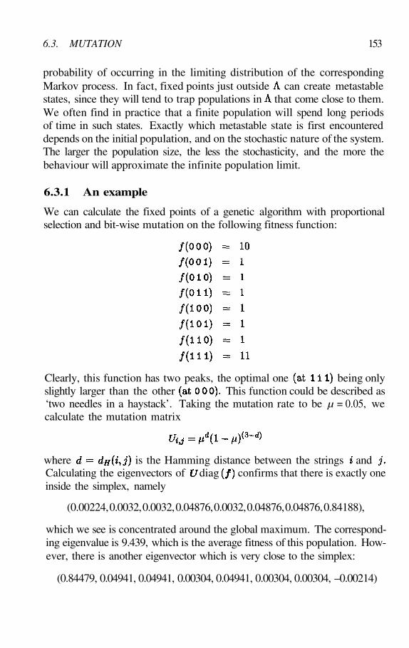
6.3. MUTATION 153
probability of occurring in the limiting distribution of the correspondingMarkov process. In fact, fixed points just outside can create metastablestates, since they will tend to trap populations in that come close to them.We often find in practice that a finite population will spend long periodsof time in such states. Exactly which metastable state is first encountereddepends on the initial population, and on the stochastic nature of the system.The larger the population size, the less the stochasticity, and the more thebehaviour will approximate the infinite population limit.
6.3.1 An example
We can calculate the fixed points of a genetic algorithm with proportionalselection and bit-wise mutation on the following fitness function:
Clearly, this function has two peaks, the optimal one being onlyslightly larger than the other This function could be described as‘two needles in a haystack’. Taking the mutation rate to be µ = 0.05, wecalculate the mutation matrix
where is the Hamming distance between the strings andCalculating the eigenvectors of diag confirms that there is exactly oneinside the simplex, namely
(0.00224, 0.0032, 0.0032, 0.04876, 0.0032, 0.04876, 0.04876, 0.84188),
which we see is concentrated around the global maximum. The correspond-ing eigenvalue is 9.439, which is the average fitness of this population. How-ever, there is another eigenvector which is very close to the simplex:
(0.84479, 0.04941, 0.04941, 0.00304, 0.04941, 0.00304, 0.00304, –0.00214)

154 CHAPTER 6. THE DYNAMICAL SYSTEMS MODEL
This is close to the suboptimal point. The argument above tells us that anyfinite population that is close to either of these fixed points is likely to staythere for a considerable time. In the infinite population limit, of course, allpopulations will converge on the first of these. The existence of the secondone so close to the simplex however has an important influence on finitepopulation behaviour. Running a GA on this problem with a populationsize of 200 illustrates this effect. We start with an initial population closeto the second fixed point by taking 160 copies of and 20 each ofand giving a population vector (0.8,0.1,0.1,0,0,0,0,0). On a singlerun, we plot the distance between the current population and each of thetwo fixed points. We measure the distance between two vectors by
The results of a typical run are show in Figure 6.6. We can see that thepopulation stays close to the metastable region for approximately 200 gener-ations. This result will vary from run to run owing to the stochastic natureof the system.
6.3.2 Diagonalization
The maximum number of eigenvalues that a matrix can have is . Ifhas a full set of distinct eigenvalues, then the corresponding eigenvectors
are linearly independent. If we create a matrix whose columns are theeigenvectors of , then it can be shown that is a diagonal matrix,whose diagonal entries are the corresponding eigenvalues. is said to bediagonalizable. The set of eigenvectors forms a basis for the vector space onwhich operates and, in this basis, becomes a diagonal matrix.

6.3. MUTATION 155
Now suppose that diag is diagonalizable, i.e., we have found all theeigenvalues and they are distinct. It would seem that should be naturallydescribed in the basis of eigenvectors. Let be the matrix containing theeigenvectors as columns, so that where is avector containing all the eigenvalues. Given any vector x, we can expressit in the new eigenvector basis as So transforming the evolutionaryequation into this basis we obtain the following:
To proceed further, we use an alternative expression for Letbe a function of vectors which adds up their component values:
so that implies that Then
The following lemma will be useful:
Lemma 6.4 Let be a matrix whose columns sum to 1. That is1 for each Then for all
Proof
Now the mutation matrix U has the property that its columns sum toone, as does the matrix Z if we have scaled the eigenvectors appropriately.Therefore

156 CHAPTER 6. THE DYNAMICAL SYSTEMS MODEL
Putting everything together, suppose we have a population vector attime so that
Let be the same population expressed in the new basis.Then we have
Clearly, this equation is identical to the one that we derived for proportionalselection only! The only difference is that now we have a ‘fitness’ vectorwhich contains the eigenvalues of diag . This means that the dynamicsof the infinite population genetic algorithm under mutation and fitness-proportional selection with fitness vector is identical, in the new basis, tothe dynamics of proportional selection on its own with fitness vector Butwe already know how to solve the dynamics of proportional selection. Wecan apply the same result now:
remembering that represents the population in the eigenvectorbasis.1.
We can use this result to study the infinite population dynamics for thesystem in the previous example (the ‘two needles in a haystack’ problem).Transforming co-ordinates to the Z basis, we plot the proportion of eachof the two eigenvectors (optimal and metastable) found at each generation,starting with the same initial population as before. The results are shownin Figure 6.7. It can be seen that the population is expected to switch fromone to the other between generations 50 and 100. Remember, though, thatthis is for the infinite population. The effect of having a finite populationsize is to make the population stall in the region of the metastable state fora much longer time, as the experimental results in Figure 6.6 show.
1A form of this result appears in [284]

6.3. MUTATION 157
What exactly does this change of basis mean? We can illustrate what ishappening by returning to an earlier example:
The effect on the dynamics of setting µ = 0.05 and µ = 0.1 are shownin Figure 6.8. We observe that as mutation increases, so one of the fixedpoints moves inside the simplex (this is the leading eigenvector, as predictedby Perron-Frobenius) while the others move out. The extent to which theymove depends on the mutation rate: the higher the rate, the further theymove. Fixed points staying close to the simplex may form metastable stateswithin it. Note that the three fixed points form a triangle. The flow within
We have already seen that with no mutation, the fixed points are the verticesof the simplex. We now add mutation. Suppose there is a probability µ thatan individual will mutate. If it does so, then it becomes one of the otherindividuals with equal probability, generating the mutation matrix

158 CHAPTER 6. THE DYNAMICAL SYSTEMS MODEL
this triangle looks rather like the flow under selection in the simplex, butfor a different fitness function—the function comprising the eigenvalues of
diag . This is what the transformation Z means. It maps each of thefixed points back to the vertices of the simplex, and simultaneously mapsthe flow of the dynamical system inside the fixed point triangle into a flowin the simplex. This flow corresponds to a selection-only flow with the newfitness function.
6.4 Crossover
We now seek to define the action of crossover on a population vector. Thatis, we wish to define an operator such that the th component of
is the probability that individual results from applying crossover
cross to form is as sketched previously in Chapter 3. For example,with uniform crossover defined on bitstrings of length 3,
The probability that is created by applying crossover to a population isthen found by summing over all the possible ways this can happen:
Sometimes crossover is symmetric, so that as with uni-form crossover, for example. However, even if crossover is not symmetric,we can define symmetric matrices having component
It is straightforward then to check that
Each component of is a quadratic form, and itself is a quadratic operator.As an example, consider bitstrings of length 2, and one-point crossover,
where we allow crosspoints before the first and after the last bit2. We2We recognize that this choice of crosspoints is rare in practice, as it leads to cloning,
but we need it for this illustration. Otherwise we would need longer strings and thematrices would be rather large!
to population Suppose and that the probability that these two

6.4. CROSSOVER 159

160 CHAPTER 6. THE DYNAMICAL SYSTEMS MODEL
associate the search space with the integers usingthe standard binary representation. therefore is the probability that
and cross to form The following table gives the different valuesof
It can be seen that one-point crossover is not symmetric since, for example,
However, we can take the matrix to be symmetric and still obtain thecorrect quadratic form for
Doing this for each gives us
where each is symmetric.It should be noticed that this means that different crossovers might lead
to the same operator indicating that they have identical effects on apopulation. For example, suppose we have two different forms of one-pointcrossover. The first one generates a single offspring from the left-hand endof one parent and the right-hand end of the other parent. The second onegenerates both offspring and selects one of them at random. It can bechecked that both of these crossovers have the same corresponding set ofsymmetric matrices and that therefore their effect on populations isidentical. (A similar effect in the case of permutations is demonstrated byWhitley and Yoo [309].)
6.4.1 Mixing
If we combine crossover with mutation we obtain the mixing operator

6.4. CROSSOVER 161
where mutation is applied to parents before crossover. For a large classof independent mutation operators (including all the standard ones on bit-strings), it doesn’t matter whether mutation is applied before crossover orafterwards [293]. The mixing operator also turns out to be a quadraticoperator [243]:
where is the mutation matrix. Some of the properties of that relateto the structure of the search space will be described in the followingsection.
The full sequence of selection, mutation and crossover gives us the com-plete operator for the genetic algorithm:
If selection is proportional to fitness then, as we have seen,
One of the properties of quadratic operators such as is that, for anyvector and scalar
From this it follows that, for proportional selection
and so we obtain
for each which gives us the complete equation for the genetic algo-rithm. Iterating this equation gives us the infinite population trajectory forthe genetic algorithm with proportional selection.
As in the case of selection and mutation, the dynamics of a finite popu-lation genetic algorithm with crossover are strongly influenced by the fixedpoints of the infinite population system [290]. It can be shown empiricallythat in many cases the finite population spends most of its time in the vicin-ity of a fixed point. It eventually escapes and quickly becomes captive toanother. It sometimes happens that whole regions of the simplex can stall

162 CHAPTER 6. THE DYNAMICAL SYSTEMS MODEL
the population. If the force of is small on a connected subset then thepopulation will drift randomly around it until it manages to escape. Suchregions are often referred to as neutral networks, as the average fitness ofthe population does not alter significantly within them, and it appears thatthey may constitute manifolds of the infinite population fixed points. How-ever, there is as yet no known method for analytically determining the fixedpoints of a genetic algorithm with crossover, and so most investigations ofthis phenomenon are either empirical, or relate to carefully constructed fit-ness functions. It should be noted that the fixed points may well containcomplex numbers. These may still be ‘close’ to the simplex, if our notion ofdistance is extended appropriately. They are just as important as real-valuedfixed points in understanding the dynamics of the system.
Analysing the properties of is difficult and there are many open ques-tions. Two important issues concern the convergence of iterates of Weshall say that is focused if it is continuously differentiate and its iteratesalways converge to a fixed point. The differentiability of is not a prob-lem, but little is known about conditions under which the iterates converge(as opposed to forming a periodic orbit, for example). It is known that,when there is no crossover, convergence to a fixed point is assured. Withcrossover, the situation becomes more complicated. When the search spaceis and in the case of linear fitness functions and no mutation, it isknown that is focused [289]. A perturbation argument shows that thiscontinues to be the case for small mutation rates and nearly linear fitnessfunctions. However, it is possible to define pathological forms of mutation(which are not used in practice) for which periodic attractors are found [315].Certain forms of ‘self-adaptive’ mutation schemes can produce periodic oreven chaotic behaviour [317]. Finding precise conditions for to be focusedis thus an important open question.
The second issue concerns whether or not the fixed points are hyperbolic.A fixed point is said to be hyperbolic if the differential of at the pointhas no eigenvalue with modulus equal to 1. Hyperbolicity is an importantconcept in determining the stability of fixed points. It is known that for thesearch space of binary strings, with proportional selection, bitwise mutation(at a positive rate) and any crossover, fixed points are hyperbolic for almostall fitness functions.3 However, it is an important open issue to generalisethis result to other search spaces, and to the operators that act upon them.
3More precisely, the set of functions for which this statement is true is dense in the setof all fitness functions.

6.5. REPRESENTATIONAL SYMMETRY 163
6.5 Representational Symmetry
In this section we shall investigate the relationships that exist between struc-tures within a search space and the operators (crossover and mutation) thatact upon them. These properties of will be analysed from a purely syn-tactic viewpoint, by considering the way in which crossover and mutationact on structural properties of the representations of points in the searchspace. Whether or not these operations make sense semantically (that is, interms of the fitness of the points) is a difficult and fundamental open ques-tion. At present, the best we can say is that if our knowledge of the searchproblem at hand leads us to think that a certain representation is sensible,then crossover and mutation can act on that representation in certain in-teresting ways. Moreover, this can lead to a simplification of the equationsdescribing the dynamics of the infinite population model.
Suppose we have selected a particular representation in order to obtainour search space There may be various structures and symmetries im-plicit in this representation. Indeed, if there is no such structure, searchingthe space will amount to random sampling. An example of such a structureis the notion of a landscape, which we shall consider in greater detail inChapter 9. We might choose a representation so that points of the searchspace correspond to vertices in a graph. Neighbouring vertices (joined byan edge) correspond to points in the search space that are similar in somesense. For example, the set of fixed-length binary strings can be thoughtof as forming a graph in which neighbours are points that are Hammingdistance 1 apart. We can model such structures and their symmetries byconsidering permutations of the search space (i.e., bijections acting on )that preserve the structural properties in which we are interested. In thecase of the landscape graph, such a permutation would have to map ver-tices in such a way that if two vertices were connected by an edge, then sowould be the images of these vertices. The collection of such permutationsrepresent the different ways in which points of the search space could berelabelled, whilst preserving the essential structural properties.
These structural symmetries may be describable mathematically in termsof a group that acts on the search space [244]. We denote this group by
It comprises a set of permutations of which satisfies the followingconditions:
1.
2.
The identity permutation is in L.
If then the inverse permutation is also in L.

164 CHAPTER 6. THE DYNAMICAL SYSTEMS MODEL
3. If and are in L, then so is (where is the group operation).
We shall assume throughout that this group acts transitively on that is,for any there exists some such that
A special case of a group acting on is when itself forms a group.For example, the set of fixed-length binary strings forms a group under theoperation of bitwise addition modulo 2. A second example is when is aset of permutations (as in the travelling salesman problem), for which thegroup operator is composition.
We can identify permutations of with permutation matrices that acton For each we may define a matrix by
It is easy to check that this is equivalent to defining
Note also that the set of matrices forms a group undermatrix multiplication that is isomorphic to
We say that the mixing operator commutes with ifWhen this happens, the definition of simplifies
considerably. Recall that is defined by matrices:
If mixing commutes with then, for each let be apermutation such that Then
In other words, the probabilities in each matrix are exactly those thatare in but shuffled around according to the permutation matrixWe have already touched on the benefits of this property in Chapter 3: therelationship between mixing (crossover and mutation) and the structuralsymmetries of lead to a simplification in the mathematical expression for
All the relevant probabilities are stored in one matrix which iscalled the mixing matrix. We therefore only have to calculate this matrixin order to capture the whole effect of crossover (and mutation).
What kinds of crossover and mutation have this property? From thedefinition of crossover, it is clear that the relation

6.5. REPRESENTATIONAL SYMMETRY 165
will give this result. That is, the action of crossover must be invariant withrespect to the relabellings which preserve the structures of the search space.Similarly, for mutation we require
Firstly, it can be seen that we have used the symmetric versions of thematrices as explained previously. Secondly, note that each matrix has thesame collection of probabilities, shuffled around. The natural group actionon this search space is to consider itself as a group under bitwise additionmodulo 2. The group table for this is
The element is the identity in this group. The correspondingpermutation matrices are
We can now continue with the example of in the case ofWe have already calculated The complete set of matrices for this
crossover operator is

166 CHAPTER 6. THE DYNAMICAL SYSTEMS MODEL
The mixing operator for this crossover commutes with the group, whichmeans that
for each What this means in terms of the effect of crossover on twostrings is as follows. Consider the probability that crossing with willproduce There is only one way to do it: put the crosspoint in the middleand combine the first element of the first parent with the second elementof the second parent. Now consider the probability of crossing withto produce We have an exactly symmetric situation. The two parentstrings are complements and we need to combine the first element of onewith the second element of the other. It is these symmetries that the groupaction is describing. From the group table we can see that to relabel soit becomes we have to ‘add’ the string Applying this action to thewhole example shows that they are symmetric:
It is simple to check that bitwise mutation also commutes with this group.
6.5.1 Schemata
Once we have a group that acts transitively on the search space, and whichcommutes with mixing, it is interesting to consider the relationship betweenthe detailed structure of the group and the genetic operators. In particular,we are interested in the subgroup structure. A subgroup is a subset of thegroup that is also a group in its own right. To simplify matters we shallonly look at the case of fixed-length binary strings, although the resultsgeneralise to other search spaces. Consider binary strings of length 5, withbitwise addition modulo 2. Here is an example of a subgroup of this group:
Adding together any two strings from this set gives us another member ofthe set. The identity element is also in this set. Note alsothat this set corresponds to the schema In general, any subgroupof corresponds to a schema. If we now add the element toeach element in the subgroup, we obtain the following coset of the subgroup
6.5. REPRESENTATIONAL SYMMETRY 167
which corresponds to the schema In general, if we have a sub-group then a schema is any set
for any We are interested in schemata here because of theirintrinsic relationship to the structure of the search space. If these sub-group symmetries are important to us then we might wish to construct acrossover operator that preserves them. Using the terminology introducedby Radcliffe [198], we shall say that crossover respects a set if, when-ever two parents are chosen from S, the offspring is guaranteed to be in Salso. We are therefore particularly interested in crossover operators thatrespect schemata. In the case of binary strings, there is an important classof crossovers that have this property, defined in terms of a binary maskaccording to some probability distribution, as described in Chapter 2. Wethen assemble the offspring from the parents according to that mask. Forexample, if we have parents and the maskindicates that we should take the first three bits of the first parent and thelast two bits from the second parent to produce This string isa member of the schema as were both parents: this schema hasbeen respected by the action of crossover. We obtain different crossover op-erators according to the probability distribution over masks. It is easy to seethat all the usual crossovers on binary strings can be definedin this way. It can be proved that any crossover defined by masks preservesschemata for binary strings. Moreover, this result can be generalised to aclass of search spaces called structural spaces. The corresponding crossoveroperators are called structural crossovers and they can be shown to respectthe schemata given by the underlying subgroup structure [245].
It should be emphasized that schemata correspond to structural proper-ties of the search space, without reference to the fitness function. There istherefore no guarantee that choosing a crossover that respects them will givea useful operator for any specific search problem. At present there is littletheory to relate the structures implicit in a representation to properties ofthe fitness function. Choices of representation and operators must be madeby the practitioner on the basis of whatever is known (or guessed) about theparticular problem to be solved. The theory of genetic algorithms cannot atpresent guide this choice, but simply analyses the connections between thechoices of representation and operators. The problem of analysing struc-tures within a particular fitness landscape is addressed in Chapter 9; it ishoped that, eventually, a theory will be developed to connect the representa-

168 CHAPTER 6. THE DYNAMICAL SYSTEMS MODEL
tion/operator question with fitness issues. This remains perhaps the singlemost important research topic in the study of genetic algorithms.
The most obvious attempt to address this issue is of course the SchemaTheorem. As we have discussed at length in Chapter 3, this attempts totrace what happens to members of a particular schema from one generationto the next [124]. Although we have just seen that schemata arise naturallyin the study of crossover, problems immediately arise in trying to definethe action of selection (the operator related to fitness) on a schema. It isusual to define the fitness of a schema to be the average of all members of apopulation belonging to that schema. However, this gives us a definition thatis a function of the particular population (and therefore implicitly a functionof time). We cannot, therefore, study what is happening to a particularschema without keeping track of what is happening to the entire population.The Schema Theorem does not buy us anything in terms of theoreticalunderstanding and analysis without a great deal of further work [273, 274,297].
6.5.2 Walsh transforms
As we shall see in Chapter 9, one approach to the analysis of a fitnesslandscape is in terms of its Fourier transform. The relationship betweenthe Fourier transform of a fitness function and the ability of operators tosearch on the corresponding landscape is not well understood. However,this technique does simplify the mixing equations in a remarkable way. Inthe case of fixed-length binary strings, the Fourier transform is actually theWalsh transform.
We have already introduced this transform in Chapter 3; here we use aslightly different version of the matrix that represents the Walsh trans-form. We denote this by
where is an inner product.4 Since W is a real symmetric orthogonalmatrix, it is therefore its own inverse, i.e.,
4The use of the factor is for reasons of symmetry in defining the inverse transform.In this form the Walsh coefficients differ from the definition in Chapter 3 by a multiplicativeconstant.

6.6. BIBLIOGRAPHIC NOTES 169
A key property of the Walsh transform is that it simultaneously diagonalizesthe permutations matrices That is is a diagonal matrix for each
This enables the mixing operator to be simplified:
Thus we have the product of the Walsh transform of the mixing matrix withtwo diagonal matrices. This is a rather efficient way to calculate More-over, it also allows results concerning the inverse of and its differentialto be obtained [292].
If our search space comprises fixed-length strings in which each posi-tion has its own finite alphabet, then a more general transform (the Fouriertransform) can be defined which again diagonalizes the associated permu-tation matrix group. However, it turns out that such spaces are essentiallythe only ones for which this can be done. The crucial factor is that theunderlying groups for such spaces are commutative (i.e., for allelements ). Indeed, any commutative group has a representationof this form (although the crossover operator need not be defined by maskswith respect to this structure). However, when the group is not com-mutative (for example, the group of permutations in the travelling salesmanproblem), there is no matrix transform that will diagonalize its matrices.
Given that the Fourier (or Walsh) transform unravels the action of mix-ing in such an elegant way, and, moreover, that the very same transformcan be used to analyse the structure of fitness landscapes, it gives us somehope that this will provide a fruitful avenue for exploring the relationshipbetween particular fitness functions and the genetic operators that act uponthem.
6.6 Bibliographic Notes
The study of GAs as dynamical systems has been primarily developed byMichael Vose. His book The Simple Genetic Algorithm is a comprehensivedescription of this theory, applied to search spaces of fixed-length binarystrings [293]. This book is essential reading for anyone interested in under-standing genetic algorithm theory.
The dynamics of the genetic algorithm with selection and mutation hasbeen extensively analysed by researchers at the Santa Fe Institute, on a

170 CHAPTER 6. THE DYNAMICAL SYSTEMS MODEL
range of fitness functions[284]. Their work emphasizes the view of evolutionmoving along neutral networks in metastable regions and then escaping tonew regions. The Z transformation mapping the flow of a selection plusmutation algorithm to that of a pure selection algorithm is also based ontheir work. Some interesting results for selection and mutation acting onfunctions of unitation can be found in a paper by Jonathan Rowe [242].
This emergent view of population dynamics has also been propoundedby Vose. He has described the long term behaviour of a genetic algorithmas taking place on a graph, in which the vertices correspond to metastablestates, and the edges the transitions which can occur between these states.There is, as yet, no general analytical way of constructing this graph, andthis remains an important open question.
The analysis of mixing (crossover and mutation) is again based on Vose’spresentation. That a mixing matrix might exist for other search spaces wasshown by Vose and Darrell Whitley [296]. The more general investigationof the links between group symmetries of the search space and the actionof mixing has been developed by Jonathan Rowe, Michael Vose and AldenWright [244]. The concept of respect, which this paper builds on, was intro-duced by Nick Radcliffe [198, 202].
The relationship between mixing and the Walsh transform was analysedby Vose and Wright for binary strings [292]. The proof that such a transformdoes not exist for non-commutative groups is in a paper by Rowe, Vose andWright [245]. Further generalisations can be made—for example, to searchspaces with variable-sized structures, as in Genetic Programming (see thework of Riccardo Poli [189] for details). Related work by Chris Stephenshas tried to reconcile the dynamical system view of genetic algorithms withthe Schema Theorem [273, 274].
Exercises
1.
2.
3.
Show that Theorem 6.2 holds for both proportional and rank selection(with ties broken randomly). For arbitrary selection, describe sufficientconditions for this theorem to apply.
Write down the operators and for the genetic algorithm describedin Exercise 5 of Chapter 5. Find the fixed points of the infinite popu-lation system. Compare your findings with the experimental results.
Parameterized uniform crossover is defined in a similar way to uniformcrossover, except the probability of a bit being taken from parent 1 is

6.6. BIBLIOGRAPHIC NOTES 171
4.
5.
6.
and the probability that it should come from the second parent iswhere is a parameter of the operator. (‘Standard’ uniform
crossover corresponds to setting .) Write down the mixingmatrix for this kind of crossover in terms of for binary strings oflength 2. Remember that the mixing matrix should be symmetric.
Write down the mutation matrix for binary strings of length 2, witha bitwise mutation rate of µ . Calculate the Walsh Transform of themutation matrix, What do you notice about this matrix?
Write down the mixing matrix for binary strings of length 2, withuniform crossover. Calculate the Walsh Transform of the mixing ma-trix, What do you notice about this matrix?
Suppose we have a fitness function on fixed-length binary strings.Calculate the Walsh Transform of diag showing that thecomponent of this matrix is
where is the Walsh Transform of the fitness function. Whatdoes this tell you about the problems of handling selection in the Walshbasis?

This page intentionally left blank

Chapter 7
Statistical MechanicsApproximations
The equation that we analysed in the previous chapterdescribes what happens to a population in a single generation of a geneticalgorithm. It tells us exactly what the probability distribution over all possi-ble next populations is. In the infinite population limit, it tells us the exacttrajectory of the population in all subsequent generations. The population
is a vector in space, and so we really have equations, onefor each element of the search space In practice, of course, is extremelylarge and we have a large number of equations to solve if we want to deter-mine the trajectory of This task rapidly becomes impracticable as thesize of the search space grows, so it is natural to investigate methods forobtaining an approximation.
7.1 Approximating GA Dynamics
The situation is analogous to one that is often encountered in physics, inwhich there is a system comprised of many components interacting together.Although we might be able to write down the equation describing eachcomponent, there are so many that it is impossible to calculate what happensto the system as a whole. For example, consider a balloon containing somegas. There are so many molecules moving around inside the balloon that itseems hopeless that we shall ever be able to calculate what happens to theballoon as a whole, even if we were given precise information about the stateof each molecule. The way to proceed, of course, is to look at average valuesof the whole system. While we may not be able to predict which molecules

174 CHAPTER 7. STATISTICAL MECHANICS APPROXIMATIONS
strike the surface of the balloon at any one time, we can work out on averagehow many will do so, and we can summarise this in a single quantity, thepressure of the gas. Similarly, the average velocity of each molecule can besummarised by the temperature of the gas. In this way, we can describe thesystem as a whole with a couple of parameters, instead of the many requiredto describe each individual molecule. The branch of physics that deals withsuch averaging processes is called statistical mechanics.
We might therefore hope to describe a genetic algorithm using a similarapproach [196, 263]. If we can identify certain average properties of the pop-ulation, then we might be able to write down equations for these properties,and use these to find out the trajectory of the system as a whole. Of course,in reducing the system to a few average properties we are throwing awaya lot of information, and strictly speaking we obtain an approximate resultonly. The hope is that deviations from this approximation will be relativelyrare. In the case of the balloon, it is a possibility that all the moleculesin the balloon might all at some time be on one side of the balloon. How-ever, this state of affairs is so unlikely that it seems safe to disregard it. Ifwe assume that our genetic algorithm uses an infinite population, we cansimilarly disregard fluctuations. As we have seen, in the infinite populationlimit, the genetic algorithm behaves deterministically. We shall thereforecontinue to assume that the population is infinite for the moment.
However, if the population is small, then we shall no longer be ableto ignore these effects. If the balloon were to contain only two molecules,the chance of both of them being on one side of the balloon is quite high.Similarly, we shall have to consider fluctuations caused by having a finitepopulation. We shall do this by viewing them as sampling effects, whichcause the population to deviate from the infinite population trajectory.
So how do we go about finding a suitable small set of parameters that(approximately) describe the state of a genetic algorithm? The full system isdescribed by the variables, where is the proportion of thepopulation occupied by element of the search space. We can view thesevariables as describing a probability distribution over the search space. Themapping gives us another such distribution. So we need a good way ofapproximating distributions.
A well-known method for approximating continuous functions of a realvariable is to look at their Fourier series. Any continuous periodic functioncan be expressed as an infinite sum of sine and cosine functions. For example,consider the function on the interval We can calculate

7.1. APPROXIMATING GA DYNAMICS 175
the Fourier series of this function to be
or
Clearly, as the series is expanded, the terms correspond to higher and higherfrequencies, and have smaller and smaller coefficients. We can think of thefirst few terms as providing an approximation to the curve and thelater terms as giving small corrections (see Figure 7.1).
The distributions that we wish to approximate are not continuous, butdiscrete. However, we shall see that a similar approach can be used in thiscase. We shall show that the population equation can be written as aninfinite series with ever decreasing coefficients, and that we can thereforeapproximate the characteristics of the infinite population by truncating thisseries. It may seem a backward step to express a set of variables usingan infinite set of coefficients. The trick is, of course, that we shall truncatethis series to obtain an approximation using far fewer than terms. Theseleading coefficients will be our summary statistics with which we shall trackthe trajectory of the population.

176 CHAPTER 7. STATISTICAL MECHANICS APPROXIMATIONS
7.2 Generating Functions
Suppose we have a random variable that can take non-negative integervalues. For each there is a certain probability that takes the value
The probability distribution for can be described by its probabilitygenerating function
For example, if we have a population vector then thecorresponding probability generating function is
This polynomial contains complete information about the population Wecan therefore work just as well with these functions as with the populationvector itself. It is easy to see that for any probability generating function
and that its derivative is
so that
To proceed to our goal of expressing the population distribution as an infiniteseries, we use the substitution of variables
which gives us the characteristic function of the distribution
If we expand the characteristic function as a Taylor series in we obtain
where the numbers are called the moments of the distribution, beinggiven by
If we are given we can find the moments by differentiating an appro-priate number of times and setting

7.2. GENERATING FUNCTIONS 177
7.2.1 Cumulants
Is this the infinite series we are looking for, by which we can approximateour population Unfortunately not! The problem is that the momentsgrow larger and larger, not smaller and smaller, since Insteadwe look at a related function, called the cumulant generating functionand its Taylor series:
The coefficients are called the cumulants of the distribution. There isa series of formulae for converting between moments and cumulants, whichstarts like this:
We see that the first cumulant is the mean of the distribution, and thesecond is the variance. The Gaussian (or Normal) distribution is com-pletely defined by its mean and variance and all the higher cumulants arezero. Any distribution with very small values for the higher cumulants willlook rather like a Gaussian. This, then, is the infinite series that we shalluse to approximate populations. As long as populations are distributed ap-proximately normally, we shall be able to truncate the series expansion anduse just the first few cumulants.
Although the definition of cumulants looks a lot uglier than that formoments, they are in fact much simpler to use. The main reason for this isthat they have the property of linearity: if we know the for each of twoindependent random variables and , then
so that the cumulants for the random variable can be found simplyas a sum
a property that is true for moments only in the case of This property ofcumulants will prove very useful later.1
1 More information on probability generating functions and cumulants can be found inChapter 8 of [105].

178 CHAPTER 7. STATISTICAL MECHANICS APPROXIMATIONS
The first problem we face in using this approach is to decide what therandom variable should be. In the definition of the probability generatingfunction given above, we took it that the variable was ranging over thesearch space However, when thinking about the effects of selection, itis more convenient to think of as taking on the different possible fitnessvalues. In other words, must range over
Although this choice is convenient for selection, it is not necessarily useful forhandling mutation and crossover. These operators act on the structure of theelements of the search space, independently of the fitness. This dilemma isreally the same problem that we came across in the last chapter. The effectsof mutation and crossover are syntactic (they affect the structure of elementsof ) while the effect of selection is semantic (it depends on the ‘meaning’of an element, as described by the fitness function). To make life simplewe shall concentrate on the one particular case where there is no (or little)distinction between the two: the Onemax problem. Here, our search spaceis the set of binary strings of length and the fitness function is simplythe number of ones in the string. With this function, all we need to beconcerned about is the number of ones within a string: the unitation classof the string. We shall therefore think of our random variable as rangingover the set of possible unitation classes (Further examplesof functions defined over unitation classes can be found in Appendix A.)
Here is an example. Suppose our string length is and we have apopulation of size 20. If we generate an initial population at random, wemight obtain the following:
If we view this population as defining a distribution over the unitationclasses, we obtain

7.3. SELECTION 179
The probability generating function for is the polynomial
Making the substitution gives us the characteristic function
We can expand this as a Taylor series to generate the moments of the dis-tribution
from which we can read off the moments and so on.As can be seen, the moments grow larger and larger. Taking the naturallogarithm of gives us the cumulant generating function
Expanding this as a Taylor series gives us the cumulants
We see immediately that the mean is 2.45 and the variance 0.6475. Asmoothed version of this distribution is nearly Gaussian (see Figure 7.2),so we can approximate the population by truncating this series expansion.We might therefore only use the first three or four cumulants as our ‘macro-scopic’ variables and consider what happens to them under selection, muta-tion and crossover.
7.3 Selection
Suppose we have a population with corresponding characteristic function

180
where our random variable ranges over possible fitness values. That is,we can write
the effect of applying proportional selection to In the infinite populationlimit, this gives us a new population vector The characteristicfunction for the new population is
The probability of a fitness value appearing in the new population is
where is the average fitness in population This is just the equationfor selection that we worked out in the previous chapter. We therefore havea characteristic function
CHAPTER 7. STATISTICAL MECHANICS APPROXIMATIONS
where is the proportion of the population with fitness Wewant to know

7.3. SELECTION 181
Thus, we can find the new characteristic function by differentiating the oldone and dividing by the mean fitness. This makes it particularly easy toobtain the new moments. If we write the Taylor expansion of as
then differentiating with respect to gives us
Dividing through by then gives us the new characteristic function
so we can read off the moments of the new population
and, in general
However, we really need to use cumulants rather than moments. This isa pity in some ways because the moment equations for proportional selec-tion are so straightforward. However, we can use these formulae to convertbetween moments and cumulants, and after a little rearranging we obtain

182 CHAPTER 7. STATISTICAL MECHANICS APPROXIMATIONS
and so on. Clearly, it will become rather ugly for the higher cumulants, butfortunately it is these that we shall truncate!
Note that we have in fact derived these equations for proportional se-lection for any fitness function. Nowhere did we need to restrict ourselvesto functions of unitation. We can immediately gain some qualitative insightinto the effects of selection. The first equation tells us that the mean willincrease by an amount proportional to the variance, and inversely propor-tional to the mean of the fitness. So the greater the spread of values in ourcurrent population, the greater the increase in mean fitness. This relatesquite closely to previously known results in population genetics concerningthe response to selection, as discussed, for example in the context of theBreeder GA [175].
The second equation tells us what happens to the variance. If the thirdcumulant is relatively small, it is clear that the variance decreases by anamount that is roughly the square of the ratio of the mean and the variance.We should expect the variance to drop quickly while is small. Thisthird cumulant is related to the skewness of the distribution. This is ameasure of how much of the distribution is on one side of the mean. Itsexact behaviour is hard to predict however. In particular, as the populationconverges around the maximum the distribution may become very skewed,which will seriously compromise our approximations. If the distributionbecomes one-sided, we shall have a large number of copies of the maximumfitness value and fewer copies of smaller values, but no copies at all of highervalues. The approximation will break down at this point. However, wehope that the transient trajectory of the population up to this point will bemodelled fairly accurately.
Suppose we assume that the cumulants are zero, which givesus an approximation to the dynamics of selection using just three variables.How well does this perform in modelling the transient stage of evolution onthe Onemax problem? Firstly we need some initial values for our variables.If the strings are of length and are generated randomly, the number of onesis given by a binomial distribution of trials with probability 1/2. This givesus the following initial conditions:
We now iterate our equations to obtain predictions for the first few gen-

7.4. MUTATION 183
erations. The graphs in Figure 7.3 illustrates what happens whenThe clear prediction is that the mean should increase, the variance decreaseand the skewness quickly become zero. It is this last prediction which isalmost certainly incorrect as the population approaches the maximum, andthis will create errors in the exact predictions of the other two values. Theaverage over 200 runs of an actual GA is also illustrated in this figure. Ascan be seen, the prediction for the mean fitness is quite good for the firstfew generations (the transient phase). As the population begins to converge,however, the approximation becomes worse and worse. The variance doesdecrease, but much faster than predicted. The real problem is however,where the prediction is frankly a disaster, except that at least its value doesstay relatively small.
We have managed to predict approximately the transient values of themean for the Onemax problem under proportional selection, using threevariables only, but the predictions for the other cumulants are not so good.In particular, the whole approximation breaks down close to convergence.As Figure 7.4 shows, this is due to the population becoming more and morelop-sided as it approaches the maximum value. Happily, this problem willbe alleviated when we introduce mutation and crossover because, amongstother things, these operators have the effect of maintaining the populationdistribution closer to a bell-shaped (Gaussian) curve throughout the evolu-tionary process.
7.4 Mutation
We now add bitwise mutation to our genetic algorithm, following the de-velopment of [196]. As remarked above, this helps to keep the populationcloser to a Gaussian distribution throughout the process. This can be seenin a typical run on Onemax as shown in Figure 7.5. It is evidentthat, even when the process has converged, we still obtain a fairly symmetricpopulation. Thus, the higher cumulants stay small and we should obtain amuch better approximation than we did with selection only.
To incorporate mutation into our model we must calculate the effectsthis operator has on the cumulants of a population, and then combine theseeffects with those we worked out for proportional selection. Restrictingour attention to Onemax makes this task fairly easy. Recall that we areconsidering a random variable that ranges over the possible fitness values.We can think of the value of each bit position as being a random variablethat can take on the values 0 or 1. The fitness is then given by the sum of

184 CHAPTER 7. STATISTICAL MECHANICS APPROXIMATIONS

7.4. MUTATION 185

186 CHAPTER 7. STATISTICAL MECHANICS APPROXIMATIONS

7.4. MUTATION 187
these variables. Denoting the value of bit by our fitness variable is
If we can work out the cumulants for each then we can calculate thecumulants for simply by addition. (This follows from the helpful linearproperty that we have already mentioned.) So if we denote the cumulantsfor by we have
Note that we have to assume that the values of each bit position are indepen-dent of each other. This assumption is satisfied for Onemax, but its validityneeds re-evaluating for any problem with non-linear interactions betweenthe bits (epistasis).
If we consider a single bit position as a random variable we canfirst calculate the moments and then convert them to cumulants as before.Recall that the moments of the distribution are given by
In this case we have a remarkable property: because can only take thevalues 0 or 1 it follows that
for all values of and thus moments of all orders are equal! This simplifiesthings greatly: we only need work out the effect of mutation on the mean of
and we automatically have the result for all moments. Suppose that wehave a randomly distributed population and consider the effect of mutationon the values in a single bit position. There are two ways in which a bit canend up as 1 after mutation: it can start as 0 and then mutate, or it can startas 1 and fail to mutate. Similarly, there are two ways that the bit can endup as 1. If the probability of mutating2 is , we can compute the expectedvalue of the bit after mutation:
2Note that we can’t use our usual notation of µ for mutation rate in this chapter as itconflicts with the conventional notation for moments.

188 CHAPTER 7. STATISTICAL MECHANICS APPROXIMATIONS
(Note how the case disappears from the sum.) Now we want toexpress the mean after mutation in terms of the mean before mutation.This is simply
and so we can write
Since all the moments are equal, we can immediately write down
whereWe now need to convert from moments to cumulants, so that we can
sum them. The first one is easy, since it is just the mean. We therefore have
Thus the mean fitness of the string after mutation is
The second cumulant is, in general, given by the formula
so after mutation, we have

7.4. MUTATION 189
(The last line follows from the fact that Summing overall the bits gives us the variance of the fitness after mutation
We can similarly (if more painfully) derive a formula for the third cumulant
Before we go any further, we should ask what these equations tell us aboutthe effect of mutation. We can rearrange the equation for the mean fitnessas
This indicates that the average imitation of a string will be moved towardsthe value In the case of Onemax, of course, the unitation is the sameas fitness, but this observation holds whatever the fitness function is, if wejust think of mutation acting on the unitation.
Now we can put the mutation equations together with those for fitness-proportional selection. This will give us a three parameter approximatemodel for a more realistic genetic algorithm. Assuming once again that allcumulants higher than the third are zero, we obtain
We can now iterate these equations to obtain predictions for the evo-lution of our GA. Figure 7.6 shows the predicted values for Onemax with
together with experimental results averaged over 200 runs. This timewe see that the prediction for the mean fitness is excellent throughout. Thevariance is also fairly well predicted, although it is slightly over-estimated.The third cumulant is not so good for the first generation, but settles toa value which is again slightly over-estimated. These over-estimates arisefrom the fact that we are using a finite population of size 100. This effect

190 CHAPTER 7. STATISTICAL MECHANICS APPROXIMATIONS
will be accounted for in the following section, but even as it stands, we havea fairly impressive set of predictions considering our model uses just threevariables.
7.5 Finite Population Effects
So far we have been treating the fitness of a population as a random variablewith some probability distribution. We have estimated the cumulants of thatdistribution, and studied the way they change over time. However, in anactual run of a genetic algorithm, we have a finite population, so that weare effectively sampling our fitness probability distribution times, where
is the population size. To account for finite population effects we needto address the following question: given a probability distribution, with acertain mean, variance and higher cumulants, what will be the expectedvalue of the mean, variance and higher cumulants of a finite sample fromthis distribution? Note what we are saying here: given that we are taking afinite sample, the mean of that sample is now itself a random variable! Weare interested in the expected value of that variable, as we are for all thecumulants of a finite sample.
Naively, one might assume that the expected values of the cumulants ofa finite sample will be that same as the cumulants of the distribution fromwhich the sample is taken. However, this is not the case in general; in fact,the size of the sample affects these values. For the first three cumulants,standard results in statistics tell us that the expected values are
where the terms on the left-hand sides represent the expected values of thecumulants of a sample of size N. Evidently, only the mean is unaffectedby sample size. The use of sample statistics to take account of popula-tion size effects is one of the main advantages of the statistical mechanicsapproach [196, 263]
We can now modify our equations for selection and mutation to accountfor population size by multiplying by the appropriate factors. To illustratethe effect of this, we shall consider a GA with a rather small populationsize, N = 20. The predictions, together with some experimental results,

7.5. FINITE POPULATION EFFECTS 191

192 CHAPTER 7. STATISTICAL MECHANICS APPROXIMATIONS
are shown in Figure 7.7 (results are averaged over 200 runs). The originalpredictions from the previous section are shown as dashed lines. The pre-dictions that include finite population corrections are given as solid lines.In the case of the mean and variance, the new predictions work extremelywell. The results are not so good for the third cumulant. This is not entirelysurprising, since the effect of selection on the third cumulant depends on thevalue of the fourth cumulant, which we are ignoring. We would find a betterresult were we to include it as a fourth variable in our model.
It is also clear that the experimental results show a higher level of fluc-tuation from generation to generation than we had with a population sizeof 100. This is a second-order effect of finite populations. In the same waythat we have been considering the expected value of the cumulants for afinite sample, we could also examine the variance of these random variables.This would give us a measure of the amount of fluctuation to expect. Forexample, it is known that the variance of is roughly inversely proportionalto the sample size N.
7.6 Crossover
When it comes to modelling the effects of crossover, we immediately en-counter a problem. The trouble is that two strings with the same fitnesscan have very different effects when crossed over. For example, suppose wehave strings of length 6. The string when crossed with itself willalways remain unchanged (under all ‘normal’ kinds of crossover). However,if we cross it with the string which in the case of Onemax hasthe same fitness, we could end up with a variety of different strings. Infact, for the case of complementary strings like these we could generate anystring in the Universe with This means that we can’t simply ask for theprobability of two strings with a given fitness producing a third with somefitness. We also have to take into account the distribution of ones in thestrings. The effect of this is that the bits can no longer be considered to beindependent variables as they were under mutation, so we can’t proceed byfinding the sum of the cumulant values for the individual bits.
To model crossover properly requires that we keep track of the corre-lations between all the bit variables. We also need to consider how thatcorrelation is itself affected by the genetic operators. Pursuing this courseis possible, but complex (see, for example, the development in [196]). Weshall take the simpler option of making an approximation. Consider whatwould happen to a population if we just kept on applying crossover again

7.6. CROSSOVER 193

194 CHAPTER 7. STATISTICAL MECHANICS APPROXIMATIONS
and again. A well-known result from theoretical biology (Geiringer’s The-orem) tells us that eventually the values in any given bit position becomecompletely scrambled [90]. More precisely, if there are ones in positionthen after repeated application of crossover, the probability that any stringin the population has a one in that position is simply where N isthe population size. Furthermore, this is true for each bit position inde-pendently. This distribution is known as Robbins’ proportions, and whenthe population is distributed like this, we can indeed treat the bit variablesindependently. How does this help us with modelling a single application ofcrossover? Well, it is also known that under repeated crossover, the conver-gence to Robbins’ proportions is very fast, although the rate is different fordifferent forms of crossover. So it seems not unreasonable to use this distri-bution as an approximation even after a single round of crossover. Of course,this can go seriously wrong if we happened to start with a pathological ini-tial population—for example, suppose we always initialized the strings byputting all the ones to the left. But provided that we start with a genuinelyrandom distribution of bits, there is a good chance our approximation won’tbe too bad.3
We can now calculate the effect of crossover on the cumulants of a popula-tion using this approximation. A little thought is enough to convince us thatcrossover does not change the mean fitness at all for Onemax. Crossovernever creates more ones or zeros: it merely shuffles the bits around. If
we can write down at once that
for crossover. For the variance, recall that we are assuming Robbins’ pro-portions after crossover, so that the bit values are independent. Thus theprobability of any one bit in a string being a one is and we can vieweach string as being independent Bernoulli trials; i.e., the fitness of a stringis distributed binomially with trials and probability of having a onein each trial. The variance of such a distribution is given by
3Incidentally, for the type of ‘gene pool’ crossover [176] that works on the whole pop-
ulation, rather than on pairs of strings, this isn’t an approximation—it’s exact!

7.6. CROSSOVER 195
We can similarly find the third cumulant simply by taking the third cumu-lant of the binomial distribution and substituting in our Robbins’ proportion
We can now incorporate all these results into our previous equations for theeffects of mutation and selection and we have a three parameter model forthe full genetic algorithm on Onemax:
where Note that our assumption about crossover means thatits effect on higher cumulants completely dominates the effects of selectionand mutation. The results of iterating these equations is shown in Figure 7.8along with experimental results (averaged over 200 runs). We see a goodlevel of agreement between theory and practice, which indicates that oursimplifying assumption is reasonable. Once again, though, there is a slightover-estimation of the magnitude of the cumulants, which may be due tofinite population effects.
On examining the equations more closely, we see that both andare given solely in terms of Thus, we can reduce our set of equations toa single one, giving us the trajectory of the mean fitness:
This difference equation can be solved to give a closed form equation for themean—although a rather messy one. Of more interest is the fixed point ofthe equation, which can be directly calculated as
which is the limit value of the mean as This value is shown fordifferent mutation rates in Figure 7.9. It is clear that increasing mutationpushes the fixed point away from the optimum. However, we should be waryof drawing general conclusions from these results, based as they are on suchan over-simplification of the effects of crossover for one toy problem!

196 CHAPTER 7. STATISTICAL MECHANICS APPROXIMATIONS

7.7. BIBLIOGRAPHIC NOTES 197
7.7 Bibliographic Notes
The statistical mechanics approach to approximating genetic algorithm be-haviour was developed by Jonathan Shapiro, Magnus Rattray, Adam Prügel-Bennett, and Alex Rogers. One of the advantages of the approach is that itis possible to model a variety of selection methods, including tournament,rank and Boltzmann selection [23, 196, 263]. Adapting the method for fit-ness functions other than Onemax is difficult. Successes to date includeinteracting spin systems [195], in which the fitness contribution of a bitdepends on the value of neighbouring bits, and the ‘basin with a barrier’problem [264]. Spin systems have also been analysed by Bart Naudts [179]from a fitness landscape viewpoint. The ‘basin with a barrier’ problem isillustrated in Figure 7.10. It is like the Onemax problem but with a gap toisolate the optimum.
It can be shown that using crossover enables the population to make thejump across the barrier far more efficiently than mutation alone can manage.A rigorous analysis of running-time complexity on similar fitness functions,by Thomas Jansen and Ingo Wegener [133] has confirmed theoretically theresults of [264]. The perceptron [210] and subset-sum problems [209] havealso been modelled successfully, and a large amount of work has been done inmodelling the effects of crossover rather more accurately than we have donein this chapter. Stefan Bornholdt [27] has applied the same methodology tothe analysis of GA behaviour on NK-landscapes (described in Appendix A).
It should be noted that in a number of the papers describing this ap-proach, statistical mechanics terminology is normally used. This can be a

198 CHAPTER 7. STATISTICAL MECHANICS APPROXIMATIONS
little confusing to readers with no physics background, so a short explanationis called for. In most of these papers, what we have been calling bit valuesare referred to as spins. Moreover, instead of taking the values 0 or 1, spinsare considered to take the values -1 or +1. The analogy is with magneticspin systems in physics, in which we have a number of interacting particles,each with a different spin. Consequently, the sum of the spin values in astring lies in the range This sum (which in our examples is thenumber of ones, or unitation) is called the magnetization of the string. Inphysics, the concern is with how such systems relax into some low energystate. The GA is therefore usually discussed from a fitness minimizationviewpoint. For example, the basin with a barrier function is usually drawnupside down, and is sometimes called ‘two wells’. The notion of the entropyof a fitness (or magnetization) value is also used. This refers to the factthat some magnetization values correspond to a small set of strings (lowentropy) and others to a large set of strings (high entropy). For example,there is only one string with magnetization but there are many stringswith zero magnetization (assuming bits take on the values This mayarise in a discussion of the effect of mutation, say, in which it is said thatmutation tends to drive the population towards high entropy regions of thesearch space.

7.7. BIBLIOGRAPHIC NOTES 199
Exercises
1. Given a probability generating function
we know that Show that the variance is
2. Consider the fixed point equation for Onemax derived at the end ofsection 7.6. Show that if mutation is set to then the averagefitness at the fixed point is approximately two-thirds of the stringlength.
3. Consider the needle-in-a-haystack function on bit strings of length
where gives the height of the needle. Let be the proportionof the population on the needle (i.e. the string of all zeros) at time
(a) Show that the effect of proportional selection is
(b) Given a bitwise mutation rate of , what is the probability that astring of all zeros is not destroyed?
(c) Approximate the effect of mutation by assuming that the proba-bility of creating the string of all zeros is negligible. Write down theevolution equation combining the effects of selection and mutation.
(d) If mutation is assumed to be small, show that the fixed point ofthe evolution equation is approximately
4. (continuation) Analyse the needle-in-a-haystack problem for binarytournament selection. Assuming that mutation is very small and thatthe chance of creating copies of the needle are negligible, show thatat the fixed point the proportion of the population on the needle isapproximately

200 CHAPTER 7. STATISTICAL MECHANICS APPROXIMATIONS
5. Analyse the effect of binary tournament selection for Onemax, byassuming that the fitness distribution is Gaussian.

Chapter 8
Predicting GA Performance
From relatively early in the development of theoretical ideas about geneticalgorithms, an important aspect has been the delineation of classes of prob-lems for which GAs were thought to be especially well (or ill) suited. Wesee this first in Goldberg’s concept of deception [97]. Partly this was drivenby the need to verify the building block hypothesis, at least in a negativeway, as we have seen in Chapter 3. It was about this time that the notionof problems being ‘GA-hard’ or ‘GA-easy’ began to be used. Although theterminology recalls that of computational complexity, there were no precisedefinitions of what was meant by such terms.
Later, deception—as originally conceived—was shown to be neither nec-essary or sufficient [107] to characterise a problem as GA-hard. Other typesof problem were investigated, some involving massive multi-modality or longpaths to a single global optimum. However, the multiple local optima andthe long paths usually related either to continuous space, or to the Hamminglandscape of a discrete optimization problem, while its relevance to how aGA solved such a problem was not entirely clear. (More will be said aboutthis in Chapter 9.) Nevertheless, there is now a considerable literature onthe question of characterizing and predicting GA performance.
8.1 Introduction
In considering this question, there are two related aspects that place theemphasis slightly differently. Firstly, we can ask questions about the generaltendency of GA behaviour, with the idea of being able to identify classesof problems that GAs find either ‘easy’ or ‘hard’. It was these questionsthat were addressed in studies on deception and building blocks. However,

202 CHAPTER 8. PREDICTING GA PERFORMANCE
even should such a categorization be possible, it still leaves open the secondquestion of how we can recognize a priori that the particular instance thatwe wish to solve belongs to one class or the other. In fact, there is a sensein which the second question is more important than the first, in that ifwe could characterize and recognize the difficulty of problem instances insome way, we could use the methodology in defining classes of hard or easyproblems.
8.2 Epistasis Variance
The first serious attempt to answer the second of these questions was byDavidor [45, 46]. The central concept in these and subsequent studies isthe idea of epistasis. This idea has already been defined in general terms inChapter 1—the assumption that fitness is not related to genes in an additiveway. It can be interpreted as expressing non-linearity in the fitness function,and in seeking to measure it, the assumption is that, at least approximately,the more epistatic the problem is, the harder it is to find an optimum.
Exactly what fitness means for real organisms is—as noted in Chap-ter 1—a complex problem, but for the case of GAs it is conceptually a sim-ple matter. The epistatic nature of many familiar functions (such as thosedescribed in Appendix A) can be determined by inspection. For unknownfunctions it is harder, but were we to know the fitness of every phenotypein the Universe of all possible phenotypes, we could in principle calculatethe effect on fitness of any combination of genes. Of course, if we reallydid know the Universe, regarding it as an optimization problem would bepointless anyway, but there is at least a theoretical possibility that we mightbe able to characterize a function using only a sample of points.
If this could be achieved, and the degree of epistasis in a given problemdetermined, we might be able to decide on the most suitable strategy forsolving it. At one end of the spectrum, a problem with very little epistasisshould be easily solved by a suitable linear or quasi-linear numerical method.At the other end, a highly epistatic problem is unlikely to be solvable by anysystematic method, including a GA. Problems with intermediate epistasismight be those worth attempting with a GA. This, at least, appears to bethe assumption that has prompted the investigations that we shall considerin this chapter.
Another aspect of the investigation of epistasis is also intrinsically rel-evant to the study of GAs. As we have seen, GAs tend to place greateremphasis than other techniques on the question of representation, and a

8.3. DAVIDOR’S METHODOLOGY 203
particular choice of coding may render a simple linear function epistatic.Conversely, by choosing a different encoding function, it may be possible toreduce the degree of epistasis in a problem. It would clearly be valuable tobe able to measure and compare the epistasis existing in different codingsof the same problem. Related to this is the question of the choice of opera-tors: as we shall see in Chapter 9, it is not only the fitness function and theproblem encoding that influence its difficulty. However, we shall postponequestions of this nature for the next chapter.
8.3 Davidor’s Methodology
Davidor assumed populations of binary strings of length for which hedefines several quantities. The basic idea is that for a given population of size N, the average fitness value can be determined as
Subtracting this value from the fitness of a given string produces the excessstring fitness value
This simply re-states the fitness of all strings in with respect to thepopulation average.
Now some allele values will occur more frequently than others at eachlocus. We may count the number of occurrences of allele a for each genedenoted by and compute the average allele value
The excess allele value measures the effect of having allele a at gene andis given by
The excess genic value of string is the value obtained by summing theexcess allele values at each gene,
Finally, the epistasis value is the difference between the actual value of stringand the genic value predicted by the above analysis, which reduces to

204 CHAPTER 8. PREDICTING GA PERFORMANCE
Thus, the value measure the discrepancy between the actual fitness anda ‘linear’ model of fitness.1 Davidor went on to define a measure of ‘epistasisvariance’ that unfortunately proved somewhat difficult to interpret. In fact,his methodology has a basic flaw, as we shall see later.
8.4 An Experimental Design Approach
Reeves and Wright [217, 218] pointed out that what Davidor was attemptingwas in fact exactly what statisticians have been doing in the sub-disciplineknown as experimental design (ED).2
Davidor was implicitly assuming a linear model (defined on the genes)for the fitness of a string. We can express this model as
In conventional experimental design, the above model would actually bewritten in parametric form. For example, the model for a string of 3 genescould be written as follows:
where is the fitness of the string and the subscript denotesthe replication number (i.e. the occurrence of the string), and allowsfor stochastic fitness evaluation. If there are no stochastic effects, we can ofcourse drop the subscript .. The parameters on the right-hand side are asfollows:
1Note that we have merely followed Davidor’s original notation here; these valuesdon’t necessarily have anything to do with expectations.
2It is interesting that it was Sir Ronald Fisher who played a major part in the develop-ment of this area of statistics, just as he did in the case of population genetics, and bothhave a place in the analysis of GAs.

8.4. AN EXPERIMENTAL DESIGN APPROACH 205
In many, although not all, applications of GAs random error is not con-sidered relevant, and we merely note that this formulation allows it to betreated if desired, although in what follows we shall assume the problems tobe deterministic.
8.4.1 An example
Suppose we have a string with and that the fitness of every string inthe Universe is known. There are of course strings, and therefore 8fitness values, but the experimental design model above has 27 parameters.It is thus essential to impose some side conditions if these parameters areto be estimated; the usual ones are the obvious idea that the parametersrepresent deviations from a central value. This means that at every orderof interaction, the parameters must sum to zero for each subscript. Thisresults in an additional 19 independent relationships such as
and so on. Imposing these side conditions allows the ‘solution’ of the abovemodel—in the sense that all the parameter values can be determined if wehave observed every one of the 8 possible strings. For example, we find that

206 CHAPTER 8. PREDICTING GA PERFORMANCE
where the notation for instance, means averaging over subscripts andThe effects can be seen to be exactly equivalent to Davidor’s ‘excess allele
values’ as defined above. For instance, his so thatSimilarly, his ‘excess genic values’ are found by summing and
for each possible combination of Finally, his ‘string genic value’ isclearly
The difference between the actual value and the genic value, is thereforesimply the sum of all the interaction terms; in other words, zero epistasis isseen to be equivalent to having no interactions in the model.
8.4.2 Analysis of Variance
The normal procedure in experimental design is to perform an ‘Analysis ofVariance’ (Anova), whereby the variability of the fitness values (measuredby sums of squared deviations from mean fitness, and denoted by SS) is par-titioned into orthogonal components from identifiable sources. In Table 8.1we give a conventional Anova table for our 3-bit example, with Davidor’snotation alongside.

8.5. WALSH REPRESENTATION 207
The degrees of freedom in this table are the number of independent elementsin the associated SS; for example, in the Total SS term, only 7 of the
terms are independent, since they must satisfy the relationship
It is easy to prove (as we shall see in Section 8.5.1) that
Total SS = Main effects SS + Interaction SS.
Since Davidor has simply divided these values by a constant to obtain his‘variances’, it is hardly surprising that he finds that
Total ‘variance’ = ‘Genic variance’ + ‘Epistasis variance’
8.5 Walsh representation
As shown in [217], for the case of binary strings, this way of decomposingthe fitness of all the strings in a Universe is equivalent to the Walsh functiondecomposition described in Chapter 3. For 3-bit strings, we find3
The ‘mapping’ from the Walsh coefficient indices to the appropriate ‘effect’is given by writing the effects in what is known in experimental design asstandard order: in this case
In experimental design it is normal to list the effects from left to right, whereas in mostof the literature on Walsh functions, the convention is to read the bits from right to left.Of course, the labelling is arbitrary, and the necessary adjustment is quite straightforward.
3

208 CHAPTER 8. PREDICTING GA PERFORMANCE
The general pattern is fairly obvious—on adding another factor the next setof effects is obtained by ‘combining’ the new factor with the effects alreadylisted, in the same order. Thus in the case of a 4-bit problem, for example,the next 8 in order will be
Another way of seeing this equivalence is as follows: the ‘interaction level’of a particular Walsh coefficient is given by the number of in the binaryequivalent of its subscript, and the specific factors involved are indicated bythe positions of those For example, consider the coefficient in a 4-bitproblem: the binary equivalent of 13 is so this represents a 3-factorinteraction, and the factors participating in this interaction are numbers1, 3 and 4. Therefore measures the effect of the interaction(using the right-to-left labelling convention). The sign of the coefficient is ofcourse determined by the relevant value of as described in Chapter 3. Forexample, the sign of the component in the value of forwould be found from
(where is the parity function), while that of the corresponding componentfor would be
In what follows, we shall use whichever notation is appropriate for the pointwe are making. While Walsh notation has advantages in terms of com-pactness and general mathematical convenience, the interpretation of thecoefficients as ED effects is perhaps more transparent. The validity of thispoint was demonstrated in [217], where an analysis of Goldberg’s conditionsfor deception from an ED perspective revealed an error in his original speci-fication. (Two inequalities in [98] which should have readand had had their right-hand sides transposed.)
8.5.1 Davidor’s ‘variance’ measure
We can partition the Walsh coefficients into subsets defined by their orderof interaction.

8.5. WALSH REPRESENTATION 209
and so on, with
Thus the linear approximation of is
Davidor’s ‘variance’ measure, as modified by Reeves and Wright [218], canthen be written (suppressing subscripts and arguments for clarity) as follows:
Definition 8.1 The epistasis variance of a function is the fraction ofthe total variation in the values that can attain that is unexplained by itslinear approximation:
where is the mean value of all strings in the Universe and the sum is overall strings.
In fact, Davidor used only the numerator of this quantity; however,it is clearly in need of some form of normalization. One possibility [282]is first to standardize all values by dividing by their maximum value.Another solution [180] is to divide by However, while these wouldguarantee that its value lies in the range [0,1], the interpretation of sucha measure is not clear. Furthermore, the value would not be invariant toa translation (i.e., a change in origin), which is clearly undesirable. Froman ED perspective there is only one sensible normalization—to divide bythe overall sum of squared deviations from the mean. The value as givenabove is then translation-invariant, and has the simple interpretation that itmeasures the fraction of the total ‘variance’ not explained by linear effects.Thus, we might expect that a value near to 0 expresses the fact that thefunction is close to linear, while a value near to 1 indicates a function thatis highly non-linear. For example, for a 3-bit problem, we have
and we see that the numerator reduces to

210 CHAPTER 8. PREDICTING GA PERFORMANCE
In fact, this can be further reduced and indeed generalized. Standard EDtheory (for example, [119] or [172]) shows that sums of squared deviationscan be additively partitioned, as we mentioned above. We can demonstratethe result in this context as follows:
Proposition 8.1 Davidor’s variance measure can be written as the sum ofthe squared interaction effects; i.e.
where the sum is over all strings.
Proof From Equation (8.3) the numerator can be written as
We can expand about the first component of the sum to obtain
Now every term in the cross-product (the second line in the above for-mula) will have a subscript that can be summed over, splitting the cross-product into two parts, one of which is zero because of the side conditions.For instance (suppressing the other subscripts for the sake of clarity),
or again,
Thus the cross-product terms disappear; a procedure that can be repeateduntil all the terms in the numerator are simply squared interaction effects.
Note (1) In the Walsh representation, the epistasis variance measure canbe written as

8.5. WALSH REPRESENTATION 211
Note (2) An immediate corollary of this result is as stated in [218]: to ev-ery function with a given value of there will be many functions whose de-composition differs from only in the sign of the interaction effects. Clearlysuch functions cannot be distinguished by the epistasis variance measure.
Note (3) The idea inherent in the definition of can be extended toepistasis of a particular order. We can define the order approximationof as
where
and the corresponding order epistasis variance as
where In other words, the sequence ofvalues measures the effect of successively better approximations to the
function It is precisely this idea that underlies the Analysis of Variancedescribed in Section 8.1. We could further consider the differencesas measuring the components of variance: the amount of variance due tointeractions of order (For convenience, we may define in orderto extend this formula to all values of )
It might seem therefore that this idea provides an excellent way of dis-tinguishing between functions with different levels of epistasis, but there aresome problems that cannot easily be resolved.
8.5.2 Signs matter
Assuming for the moment that we can obtain a good estimate of the epistasisvariance, its value still does not contain enough information to say whetherthe problem is hard or easy. In [218] the importance of the signs of theinteraction effects is pointed out. If the interaction acts counter to the jointinfluence of its associated main effects, we have essentially what we havepreviously called ‘deception’. On the other hand, no matter how large aninteraction effect is, if its sign reinforces the message of its associated maineffects, there is no deception. Figure 8.1 illustrates this point.

212 CHAPTER 8. PREDICTING GA PERFORMANCE

8.5. WALSH REPRESENTATION 213
In the upper diagram of this figure, each gene should clearly be set tohave allele 1. Epistasis exists, since the joint effect of having A and B set at1 exceeds the sum of the individual main effects, but the interaction merelyreinforces the main effects. In the lower diagram, the interaction has amalign influence: the best allele for genes A and B considered individually is1, but overall it is better to set gene A at 0 and B at 1. This would be shownby an interaction that is negative for the combination (1,1). However, thevalue uses only the square of the interaction effects, so it cannot distinguishbetween cases where epistasis helps and where it harms. A high value ofwould certainly indicate small main effects, but if the interaction effects hadthe ‘right’ signs, it could still be a trivial problem to solve.
8.5.3 Implications of sampling
As if this was not in itself a fatal blow to hopes of using as a practical toolfor measuring epistasis, there is a further problem. The whole analysis sofar has been predicated on knowledge of the complete Universe. In reality,if we knew the Universe, there would be no point in using an optimizationalgorithm, so the value of epistasis variance would be of merely academicimportance. Naturally we don’t really know the Universe, as we are typicallydealing with an enormous search space, so the temptation is clearly simplyto take a random sample and hope that is still in some sense meaningful.
Unfortunately, the meaning of depends not only on the size of thesample, but also on its composition. Reeves and Wright [218] argued that inprinciple it is not possible to estimate the value of the effects independentlyof each other from a sample. All that we can do is to estimate some linearcombination of the effects, a combination that depends upon the compositionof the sample used.
Table 8.2 illustrates the problem in the case where half the Universe isknown. For example, from Equation (8.2) the true value of would be
while the obvious estimates of both and from the half-fraction (wedenote these estimates by the ^ symbol) are
These clearly cannot be distinguished—statisticians talk of these effects be-ing ‘aliased’ or ‘confounded’. Comparing this with the true values, it is easy

214 CHAPTER 8. PREDICTING GA PERFORMANCE
to see that
In other words, all we can really do is estimate linear combinations of someeffects. What these combinations might be will be determined by the par-ticular sample we are using. In practice, we may hope that most of theinteraction effects (especially the higher-order ones) are negligible, so thatthe sample estimates we obtain will reflect the true values fairly well. Ac-tually, this assumption is at the root of most applications in experimentaldesign. However, in ED the sample would not be a random one, ratherit would be constructed on principles of orthogonality so that the task ofestimating the values of the effects that are assumed to be non-negligibleis easier. (That is, we would take care to confound the effects we are in-terested in only with those we assume to be negligible. We will say a littlemore about this in the discussion later.) In the case of experimental design,the Universe is usually rather smaller than is likely in GA applications, andin the latter case, constructing an orthogonal subset is therefore a rathermore difficult task than it generally is for ED. The temptation therefore isjust to rely on large random samples, but the sample size may need to belarge indeed if the baleful effects of confounding are to be eradicated.
8.5.4 Still NP-hard
Merely to obtain a reliable indicator of a function’s degree of epistasis is notusually an end in itself. The purpose (whether expressed or implied) is to use

8.6. OTHER RELATED MEASURES 215
this information to help us find the optimum. Whether we would still wishto use a GA is in itself doubtful. Having obtained (at some computationalcost) a substantial amount of knowledge of the function, it would seembizarre to throw it away and start again with an algorithm that ignoresthis information. The ‘obvious’ thing to do would be to try to use thisinformation directly to determine the optimal solution. But how can we usesuch information?
There is yet another difficulty here. Suppose we eventually achieve re-liable estimates of all the non-negligible effects; if we assume maximizationas the goal, we would like to be able to give + signs to all the positivemain effects, and – signs to thenegative ones. This is trivial if there is noepistasis. Unfortunately, if the function is epistatic, whether it works willdepend on how malign the epistasis is. Giving a + sign to two main effects,for example, might entail a negative influence for their associated interac-tion, so the allocation of signs is not straightforward. Essentially we havea version of the satisfiability problem to solve—an assignment of Booleanvalues has to be found that will maximize some weighted sum of ‘clauses’—and of course such problems are NP-hard [88]. As explained by Heckendornet al. [118], unless P = NP, even an exact Walsh analysis for a problem ofbounded epistasis (i.e. an upper limit on the number of factors that caninteract) is insufficient to guarantee inferring the global optimum in polyno-mially bounded time. Naudts [178] has also pointed this out, showing thatthis is the case even if the interactions are restricted to be no more thansecond-order.
8.6 Other related measures
Rochet [238] suggested the use of a quantity that she called epistasis corre-lation, defined as
where is the linear approximation to given by Equation (8.2) (subscriptshave again been suppressed for clarity). Of course, in practice this entailsfirst making estimates of the relevant Walsh coefficients in order to obtainA family of values for different orders of approximation can be definedanalogously, just as they were for In fact, is closely related to as inthe following (similar results can be proved for ):

216 CHAPTER 8. PREDICTING GA PERFORMANCE
Proposition 8.2
Proof Note, firstly, that Equation (8.3) can be formulated as
and secondly, that the effect of the side conditions on the effects is that
Thus
Equation (8.3) thus becomes
However, because of the additive partitioning of the sums of squared devia-tions
and it follows that
which is of course just another way of writing Equation (8.3). Simple algebranow shows that
and the result follows.
The consequences of this result are clear. Firstly, gives us nothingthat is not already available from Secondly, it suffers from the samebasic problem as —it is equally incapable of distinguishing between casesof benign and malign epistasis, so its value need not be indicative of problemdifficulty. The situation with respect to sampling is also as bad. Indeed, itcould be argued that the need to estimate before can be calculated

8.6. OTHER RELATED MEASURES 217
actually makes the situation worse. Certainly, if there is high epistasis inthe problem, a large sample size will be needed or else there is a high riskof confounding the estimates of the main effects with some combinationof interactions, which would mean the ‘linear model’ is biased, and theepistasis correlation obtained is seriously compromised.
Heckendorn et al. [116, 117] have proposed using Walsh sums as an al-ternative way of specifying the amount of epistasis. These are based onthe absolute values of the Walsh coefficients relating to a given order ofinteraction:
The relative size of these coefficients can be used in an analogous way to thesums of squares for although without their nice decomposition properties.However, it is clear that Walsh sums face exactly the same problem as theepistasis variance approach—they are the same modulo a change in sign ofthe Walsh coefficients, and thus cannot guarantee to tell us anything aboutproblem difficulty. (It is fair to point out that a posteriori identification ofproblem difficulty was not the main focus of the work in [116, 117].)
8.6.1 Static
Heckendorn et al. [116] also proposed a measure related to schema theory,which they called ‘static . The purpose of this measure was to assess theconsistency with which schema fitness information matches string fitnesses.For instance, if the string is optimal, then the order-2 schema fitnessaverages are consistent with this fact if
The static measure relative to a string and order- schematais given by
where is a ‘match’ function, which counts the number of loci whereand agree (e.g., ), and [expr] is the indicator function
notation introduced in Chapter 2. A combined measure of difficulty can beobtained by summing over all partitions (sets of schemata of the same order).Rana [208] shows that this measure can be quite good at predicting the ease

218 CHAPTER 8. PREDICTING GA PERFORMANCE
or difficulty of finding the global optimum. This is fine if we know wherethe global optimum is—but if we did know it, perhaps we would not be veryinterested in the abstract question of how difficult it was to find it. Also,of course, if we wish to measure consistency across all partitions, we needschema averages of all orders, which (again!) means we need to know theUniverse before we can properly compute ø.
8.6.2 Fitness-distance correlation
An obvious criticism of the epistasis variance approach is that it completelyignores the question of the search algorithm, and simply looks at the fitnessfunction. The same is true of the approach of Rosé et al. [239], who focus onthe ‘density of states’—the probability distribution of fitness values. Suchinformation may well be useful, but it says nothing about how those fitnessvalues are topologically related to each other: do they form a smooth con-tinuum4 building towards a solitary peak in the ‘landscape’ (think of MountFuji), or do they form a spiky pattern of many isolated peaks (think of theDolomites)? In fact, this will depend not only on the fitness function, butalso on the search algorithm, as we shall see at length in Chapter 9.
In the light of this, Jones and Forrest [137] suggested measuring thecorrelation between fitness and distance of sets of points on a landscapeinduced by the application of a specified operator. This is given by
where is the distance of each string from its nearest global maximum, andagain the sum is over all strings in the Universe. With some conceptof distance between solutions is now brought into play, and we can moreproperly use the term landscape. However, which distance is appropriate?The most commonly used distance measure to use for binary strings is theHamming distance, as defined in Chapter 2. However, this only defines onelandscape; other distance measures will define different landscapes, and it iscertainly not obvious that the Hamming landscape is the most appropriateone for the analysis of GAs, for example. As is pointed out in [6, 122],mutation is in some sense an approximation to the Hamming landscape,in that the effect of mutation at typically applied rates is that althoughoffspring-parent distance is technically a random variable, in practice it is
4Of course, smoothness and continuity are not really properties of discrete spaces, butas long as we understand this, such metaphors can be helpful.

8.6. OTHER RELATED MEASURES 219
often or (occasionally) 2; only very rarely is it greater than 2.However, the offspring that can be generated by crossover may be a longway from their parents in terms of Hamming distance.
In any case, also suffers from some severe problems. In the first place,the global optimum is usually unknown, so the values of are impossibleto find. In practice, we could use the fittest known string as a surrogatefor the global optimum, but there is no guarantee that the value ofthus obtained will tell us anything very useful, unless the surrogate is closeto the true optimum. On the positive side, examples of this approach inoperational research [25, 163, 224] have shown that correlations obtainedin this way are often significant, even when the distance measure is notexactly based on the operators used. There is thus a pragmatic argumentfor building algorithms that can exploit the underlying landscape structurethat seems to emerge ‘naturally’ for many COPs. But it is still not clear thatGAs necessarily induce such structure, so that measuring may not tell usmuch in general about the difficulty of a problem for a recombinative GA,in spite of the specific evidence in [137]. Indeed, several counter-exampleshave been reported [6, 197, 265].
Secondly, as with very different functions can give the same value.In order to demonstrate this fact, suppose that we create a new functionusing a quantity and a partition of the Universe of strings into two subsets,
and where
These strings subdivide further as follows:
where is the distance from to the global maximum. We use the notation
Proposition 8.3 Given a function with a single globalmaximum at the string and the transformation of as described above,the value of is unaffected by such a transformation provided that it sat-isfies the following conditions:

220 CHAPTER 8. PREDICTING GA PERFORMANCE
Proof In the first place, because we choose to increase its fitness byis still the optimal string (condition 2). It can then easily be verified thatthe value of is unaffected by the transformation. The fact thatis still the maximum, together with condition 3 and the fact that is alsounchanged (condition 4) then ensures that the numerator of Equation (8.7)remains the same. Finally, condition 1 will ensure that the denominator isalso unchanged by the transformation. Thus the value of is the same forthe new function.
An example of such a transformation is given in Table 8.3.
Note (1) Whether there is always a solution that satisfies these conditionsfor all is unknown; however, a solution has always been found for casesexamined so far. These conditions are also stricter than they need to be:even if the status of as the maximum may not change, and theother conditions will still be sufficient.

8.7. REFERENCE CLASSES 221
Note (2) Further relaxations are also possible. For example, it is only alittle more difficult to find conditions for two values and and makesimilar stipulations regarding them. In fact, since one of and canthen be chosen freely, we could find arbitrarily many functions having thesame value of Again, whether the necessary conditions can be satisfiedfor all is not known.
Note (3) This type of change is precisely that produced by a simple changeof sign for one of the coefficients in the Walsh decomposition of providedthe global optimum remains unchanged. However, if the global optimumchanges as well, may also change, whereas it makes no difference toTo this extent, fitness-distance correlation may be a more discriminatingmeasure than epistasis variance.
8.7 Reference classes
Naudts and Kallel [180] have considered the question of problem difficultyfrom a different angle. They discuss several potential measures of difficulty,including some of those mentioned above, and relate each measure to aclass of functions for which the measure attains an extreme value out of allthose possible. The value of epistasis variance, for example, will attain itsminimum (zero) for functions that are first-order or fully separable—thoseof the form
for functions that map string values to If these individual functionsare linear, we often describe as linear, but in [180] this term is givena more restricted meaning— specifically, that the fitness value is a linearfunction of the Hamming distance of the string from the global optimum.Naudts and Kallel also use a different normalization from that we use for
which leads to an ambiguity in assessing constant or flat functions (adegenerate subset of first-order functions). According to their version ofepistasis variance, there is no way to distinguish them. However, usingEquation (8.3), constant functions lead to an indeterminate value ratherthan to zero. Thus for as defined in this chapter, the reference class mustexclude the case of constant functions.
In principle, using the approach of [180] makes it possible to computethe value of a stated measure for a specified function, and compare it tothat of a member of the reference class. However, as [180] makes clear,

222 CHAPTER 8. PREDICTING GA PERFORMANCE
interpreting the resulting ratio as a measure of difficulty should be donewith caution. As well as epistasis variance, epistasis correlation and fitness-distance correlation, they discuss other concepts. Of these, we shall describeone that can be taken as characteristic of their approach.
Definition 8.2 The sitewise optimization algorithm takes an arbitrary stringand searches independently for the best allele for each gene. A sitewise op-timizable function is then one for which this algorithm delivers the globaloptimum for all input strings.
This algorithm was originally developed by Wilson [313] in an attempt todistinguish functions that were ‘GA-easy’ but difficult for hill-climbers. Forbinary strings, it simply means testing a bit-flip at each locus. Such swofunctions generalize the notion of first-order functions, which are clearly aspecial case.
Suppose we wish to use this idea to propose a measure of difficulty that isrelevant for members of the swo class. In order to define such a measure, weuse the Hamming distance metric to describe the topological relationshipsbetween vectors. The width of a set of points is defined to be the averageHamming distance between its members. Now imagine applying the swoalgorithm to a set of points; the swo measure is the ratio of the widths ofthe sets of points obtained ‘before’ and ‘after’ the algorithm is applied. Ifthe function has a unique global optimum, this measure will of course bezero.
It is also shown in [180] that swo functions are a proper subset of ‘GA-easy’ functions (if we define these in terms of schemata and deception),and of a restricted version5 of steepest-ascent (as defined in Chapter 1)optimizable functions, but that neither of these wider classes of functionsincludes the other.
From the ED perspective, first-order functions are those whose Walsh de-composition has interaction terms that are all zero, while GA-easy functionsadmit interactions, but only if they are benign. What makes for benign ormalign interactions is also discussed in [180], along with a number of otherclasses of functions and related measures, and some results concerning theirrelationships.
5The restriction lies in the fact that once the value at a locus has been fixed by thesteepest ascent algorithm, it cannot be modified again. This means that the algorithm isguaranteed to halt in no more than iterations.

8.8. GENERAL DISCUSSION 223
8.8 General Discussion
The previous sections deal with some of the flaws inherent in methods aimedat predicting problem difficulty, and attempts to correct some of the mis-apprehensions that still exist in the literature. The link with statisticalmethods also demonstrates that we need not always try to invent theoreti-cal tools from scratch: other disciplines may have some interesting light tothrow upon our subject.
8.8.1 Implications for schema theory
Turning first to the experimental design connection, it is instructive to com-pare and contrast the processes typically used in ED with Holland’s schema-processing arguments. Firstly, an assumption is made concerning the natureof the function under investigation: in particular, what is believed about themaximum level of interactions. This is then used to design a set of experi-ments that confound higher-order interactions with those of lower order sothat the effects associated with the latter can all be estimated without thealiasing problem. Then these estimates are used in order to determine thosefactors which are the most important, and those levels of each factor whichachieve the best average performance. Finally, these are combined togetherin order to provide the best overall setting of factors and levels. Furtherconfirmatory tests can then be carried out if desired, and new hypothesescan be explored based on the results of these tests.
Does this sound familiar? According to schema-processing theory, manyof these processes are in fact going on implicitly when we run a GA: implicitschema averages play the part of the explicit estimates of the effects, fitness-proportional selection does the job of sorting out which effects are mostimportant, and recombination assembles the fitter building blocks into newchromosomes that implicitly test new hypotheses.
Some experimental work reported in [225] compared several statisticalmethods for effectiveness in finding high-quality solutions to a design prob-lem. At each stage a small population was evaluated and the alleles that ap-peared to produce the worst performance were eliminated. (This was a sortof ‘stripped-down’ GA: the process was explicit and deterministic, ratherthan the implicit, stochastic approach used by a normal GA.) Differentelimination criteria were examined: using mean performance (i.e. schemaaverages) was markedly inferior to using schema maxima as the criterion.Analysis showed that deception did exist in this problem, so we would expectschema averages to provide ambiguous results. A ‘normal’ (steady-state) GA

224 CHAPTER 8. PREDICTING GA PERFORMANCE
was also run on the same problem, and it proved far more robust and lesseasy to deceive—which suggests that there is indeed rather more to GAsthan schema processing.
8.8.2 Can prediction work?
The whole idea of predictive measures raises two questions of a more funda-mental nature, however. Firstly, can we ever know for certain how difficultan optimization problem is, without exploring the whole Universe? The ar-guments of this chapter suggest that simple measures such as or justcannot guarantee to tell us how difficult a problem is on their own, evensupposing we can estimate their values reliably. We should not be surprisedthat different problems have the same values of these measures, but the situ-ation is worse in that, for any given problem, there are many closely-relatedproblems whose Walsh coefficients differ only in their signs, and epistasisvariance cannot distinguish them. In fact, by simply changing the signs ofthe Walsh coefficients [228], we can generate problems with very differentcharacteristics in terms of numbers of local optima (with respect to somespecified operator), sizes of attraction basins etc., and yet their andvalues are identical. In the most general case, therefore, we need to know allabout the Walsh decomposition in order to know how difficult the problemis. So measuring the difficulty of the problem is as hard as solving it.
Secondly (as a corollary to the above), even if we could find out, would itbe worth the effort? The presumed motivation for trying to measure problemdifficulty is to enable us to use an appropriate combination of algorithm,representation and operators. Culberson puts this dilemma neatly:
[We are] placed in the unfortunate position of having to finda representation, operators and parameter settings to make apoorly understood system solve a poorly understood problem....[wemight] be better served concentrating on the problem itself. [42]
Of course, it might be objected, this is something of a worst-case scenario.‘Real-world’ problems need not be so bad: we could focus on problems of‘bounded epistasis’—where we understand this term to mean that there areno interaction effects beyond a pre-defined order. The simplest case is thatof a first-order function, where there are no interactions of any order.
English’s information-theoretic viewpoint is clearly relevant at this point.As discussed in Chapter 4, he has shown that for almost all functions, learn-ing is hard—and it is learning that we are attempting when we aim to predictthe difficulty of solving an optimization problem. Given that optimization

8.8. GENERAL DISCUSSION 225
is relatively easy (in English’s terms), it appears that we have exchangedone problem for a more difficult one. However, we are bound to wonderwhether there is something to be learned for problems that are restricted insome way, and using the Walsh/ED representation provides an obvious wayof defining restricted classes of functions.
Culberson’s adversary argument [42], as discussed in Chapter 4, may alsobe useful here (pace English’s strictures against it [69]). In thegeneral case,Culberson’s adversary is completely unconstrained and can pass back anyvalue whatsoever. It is clear that in such cases it can also defeat any attemptto predict the difficulty of the problem on the basis of previous evaluations.At the other extreme, if the function is first-order, the adversary is highlyconstrained in its ‘evaluation’ function, and cannot report an evaluation thatis inconsistent with its past history.
Suppose then that we have a case of bounded epistasis. What sort ofalgorithm would give us the best performance? Consider an algorithmthat proceeds as follows: it repeatedly chooses a string to pass to the ad-versary, using ED principles and related assumptions about the nature ofthe function. On completing a certain number of trials is confident it hasexact estimates of all the effects so that it can predict the optimum (whichit may not necessarily have seen yet). If is correct in its assumptions,the adversary is ‘boxed in’: any future evaluations have to concur with thealgorithm’s predictions, and it cannot hide the optimum from view. Note,however, that if prediction is based on insufficient data, some at leastof the estimated effects will be incorrect, and the adversary can still falsifyits prediction, even if the assumptions as to the nature of the function arevalid. Is it possible to calculate how many trials needs before its predictioncannot be gainsaid?
In the case of a first-order function, ED theory gives some guidelines.For a string of length a ‘Resolution-III’( -III) design6
can guaranteeto compute all the main effects (i.e., order 1 Walsh coefficients) free ofconfounding. Such a design for a 3-bit problem is shown in Table 8.4.
With the half-fraction specified by the -III design, the logical estimateof is
6A Resolution- design is one in which no -factor interaction is confounded with aninteraction of fewer than factors, where Thus a -III design does notconfound main effects with each other, but main effects are confounded with2-factor interactions. In general, the existence of such designs for all is still an openquestion, and their construction is complicated, depending on group theoretic conceptsand the properties of orthogonal arrays.

226 CHAPTER 8. PREDICTING GA PERFORMANCE
which is really the value of
Thus in this case and are aliased; it is readily checked that asimilar relationship is true for all main effects. By way of comparison, theconfounding seen earlier in Table 8.2 is less neat: what we had there was alinear combination of two main effects and masquerading as simpleestimates of The important point for Table 8.4 is that for a linearfunction, the interaction terms are zero, so is a valid estimate of the truevalue In a similar way, both and can be estimated clear of main-effect aliases from this design, so that we can predict exactly the value ofany string. Of course, we want to locate the optimum without needing toevaluate every possible string, but assigning the best alleles at each locus iseasy in this case, since there are no interactions.
For the case of then, it can be seen that we choose the ‘right’subset of 4 strings to send to the adversary, it has no more room for ma-noeuvre. Furthermore, there is no subset of 3 strings that would allow usto produce valid estimates of all 3 main effects. Algorithm really is thebest algorithm we could use in this case, as it is bound to ‘defeat’ the ad-versary in the minimum number of evaluations. In general, for a string oflength choosing a design entails a maximum of evaluations, where
and finding such a design is fairly easy. Thus the growthin the number of evaluations is essentially linear in the string length. In themore general case, this merely puts a lower bound on the number of evalua-

8.8. GENERAL DISCUSSION 227
tions: if we take random samples instead of orthogonal ones, the adversarywill usually be able to keep fooling the algorithm for longer, although howmuch longer is an open question.
This sounds promising, but as so often, once we move away from thelinear case, things are considerably bleaker. As soon as we consider epistaticorder-2 functions (no interactions above 2 factors), it is already hard. Firstly, needs a design in order to compute the effects, which is rather moredifficult to construct. Secondly, even if the effects have all been computedcorrectly, we still have not solved the initial problem. As we pointed outearlier, in order to predict the optimum, now has to decide how to choosethe correct alleles at each of the appropriate gene loci, and even if we limitthe interactions to second-order, this is effectively a MAXSAT problem,which is NP-hard [118, 178].
It is true that an evolutionary algorithm such as a genetic algorithm isdifferent from our idealized algorithm GAs use random sampling insteadof orthogonal arrays, and don’t calculate the values of the effects explicitly(although schema-processing arguments suggest that it is happening implic-itly). However, it can scarcely be argued that these changes are to theadvantage of a GA, as any such implicit investigation of epistasis is likely tobe subject to greater error in its estimates of the effects.
Finally, in practice the assumption of bounded epistasis might still beincorrect. The above analysis has only asked how much data we need ifthe assumptions hold. In reality, we could use with the prescribed set offunction evaluations and thus compute all the effects up to our (presumed)maximum order, solve the satisfiability problem, and then find out that ourassumptions were all wrong. The adversary could simply make use of thealiased effects—the ones we (falsely) assumed were negligible—in order todefeat us.
8.8.3 Conclusion
The above arguments sound extremely gloomy and may suggest that notmerely the idea of investigating epistasis, but indeed the whole questionof finding near-optimal solutions to optimization problems is inherentlydoomed. From the information-theoretic perspective of English, as reviewedin Chapter 4, predicting the performance of an algorithm is really more likelearning than optimization—which means swapping an ‘easy’ problem for a‘hard’ one.
However, the lessons of years of development and practice of experimen-tal design methods (as well as GAs) suggest that the assumption of bounded

228 CHAPTER 8. PREDICTING GA PERFORMANCE
epistasis may well be a good approximation for real-world problems. Essen-tially, in many practical problems interaction effects seem to ‘die away’ quitequickly as the order of interaction grows. Thus methods based on estimatingthe size of the effects and extrapolation using some assumption about thelevel of epistasis has worked very well in practice. The ‘problem’ may wellbe mainly epistemological and not ontological—that is, although our resultsmay be entirely satisfactory, we nevertheless want to know whether they areor not, and indeed to know that we know!
Essentially, we see that really to know is usually equivalent to completeknowledge of the Universe. The idea that there is a ‘magic bullet’—analgorithm that is the best for our problem—is a nice conceit, but the effortit would need to find it is almost certainly more than we can afford. Perhapswe should drop the search for a magic bullet and use a scatter gun instead—just try to solve the problem by whatever techniques we have available. Afterall, even if we think we have found the magic bullet, in reality we can neverbe sure that we haven’t fooled ourselves!
8.9 Bibliographic Notes
Yuval Davidor [45, 46] was the first to try to characterise the epistasis ofa specific function, but it was not entirely successful. Christine Wrightand Colin Reeves made the connection to statistics and placed these ideason a firmer basis [217, 218]. Various interesting and relevant facts aboutWalsh functions can be found in papers by Rob Heckendorn, Soraya Ranaand Darrell Whitley [114, 118, 115, 117, 116]. The idea of fitness-distancecorrelation was initially introduced to GAs by Bernard Manderick and co-workers [157], and extended by Terry Jones and Stephanie Forrest [137].Further work by these and other workers is summarized in [223]. The reviewpaper by Bart Naudts and Leila Kallel [180] is also a source of much usefulinformation.

8.9. BIBLIOGRAPHIC NOTES 229
Exercises
1. Using Yates’ algorithm (see Exercise 6 of Chapter 3) or otherwise, findthe Walsh coefficients for the functions . as displayed below,and hence determine their epistasis variance.
2. (continuation) Compare the coefficients for and What do youobserve? [Hint: think of Gray codes.] What are the implications ofthis observation?
3. (continuation) Consider the signs of the coefficients for andWhat is the implication of this observation for the difficulty of opti-mizing the two functions?
4. Consider the fraction in the table below:
Verify that the ‘obvious’ estimate

230 CHAPTER 8. PREDICTING GA PERFORMANCE
actually estimates the linear combination
[Hint: Show that the coefficients in the combination satisfy the equa-tion where contains the weights used to find the esti-mate, and is the Walsh transform matrix as defined in Chapter 3.]
5. Calculate the epistasis correlation for function of Exercise 1 andverify the relationship of Proposition 8.2.
6. Calculate the value of for each of the functions of Exer-cise 1, and investigate the existence of a value as defined in Propo-sition 8.3.

Chapter 9
Landscapes
Up to this point, we have nearly always assumed (at least implicitly) thatthe topological relationship between the vectors is best described bythe simple Hamming distance. However, while this seems an obvious choicefor neighbourhood search algorithms, and for aspects of GAs that relateto mutation, it is much less obvious that it is relevant for recombination.In addition, for representations that depend on permutations, for example,whatever the choice of algorithm, Hamming distance may make little sense.This raises the whole question of what we actually mean when we talk abouta ‘fitness landscape’.
9.1 Introduction
Jones [135] was perhaps the first to stress the importance of realising that the‘landscape’ observed for a particular function is an artefact of the algorithmused or, more particularly, the neighbourhood induced by the operators itemploys. It is thus unfortunate that it is still common to find references inthe literature to the fitness landscape when it is simply the fitness functionthat is intended. Sometimes, as in the case of the so-called ‘NK-landscapes’[144], the Hamming neighbourhood is assumed, almost by default, but thisis not prima facie appropriate to GAs, for example, although it is relevantto hill-climbing algorithms based on neighbourhood search.1
With the idea of a fitness landscape comes the idea that there are alsomany local optima or false peaks, in which a search algorithm may becometrapped without finding the global optimum. In continuous optimization,
1For those unfamiliar with the idea, a description of the procedure for implementingan NK-function is given in Appendix A.

232 CHAPTER 9. LANDSCAPES
notions of continuity and concepts associated with the differential calculusenable us to characterize quite precisely what we mean by a landscape,and to define the idea of an optimum. It is also convenient that our ownexperiences of hill-climbing in a 3-dimensional world gives us analogies toridges, valleys, basins, watersheds etc., which help us to build an intuitivepicture of what is needed for a successful search, even though the searchspaces that are of interest often have dimensions many orders of magnitudehigher than 3.
However, in the continuous case, the landscape is determined only bythe fitness function, and the ingenuity needed to find a global optimumconsists in trying to match a technique to this single landscape. There is amajor difference when we come to discrete optimization. Indeed, we reallyshould not even use the term ‘landscape’ until we define the topologicalrelationships of the points in the search space In the continuous case,the detailed topology can be altered by a transformation of the underlyingvariables, which would correspond to a change of representation in discreteproblems. However, independently of the representation, the topology fordiscrete search spaces is also specified by the search algorithm with whichwe choose to search it.
9.1.1 An example
The idea that we can have a ‘fitness landscape’ without reference to thesearch algorithm is surprisingly still believed, and the contrary notion is evenconsidered by some people to be controversial. This is odd, as it is easilydemonstrated that the significant features of a landscape vary with changesin search operators and strategy. In practice, one of the most commonlyused search methods for COPs is neighbourhood search (NS), which we havealready described in Chapter 1. This idea is also at the root of modern‘metaheuristics’ such as simulated annealing (SA) and tabu search (TS)—as well as being much more involved in the methodology of GAs than issometimes realized.
A neighbourhood is generated by using an operator that transforms agiven vector into a new vector . It can be thought of as a function
For example, if the solution is represented by a binary vector (as it often isfor GAs), a simple neighbourhood might consist of all vectors obtainable by‘flipping’ one of the bits. The ‘bit flip’ (BF) neighbourhood of
9.1. INTRODUCTION 233
for example, would be the set
Consider the problem of maximizing a simple cubic function
where the solution is required to be an integer in the range [0,31]. Wehave already met this problem in Chapter 2. Regarding as a continuousvariable, we have a smooth unimodal function with a single maximum at
is easily found by calculus—and since the solution is already aninteger, this is undoubtedly the most efficient way of solving the problem.
However, suppose we chose instead to represent by a binary vectorof length 5 as described in Chapter 2. By decoding this binary vector as aninteger it is possible to evaluate f, and we could then use NS, for example,to search over the binary hypercube for the global optimum using some formof hill-climbing strategy.
This discrete optimization problem turns out to have 4 optima (3 of themlocal) when the BF neighbourhood is used. If a ‘steepest ascent’ strategyis assumed (i.e., the best neighbour of a given vector is identified before amove is made) the local optima and their basins of attraction are as shownin Table 9.1. On the other hand, if a ‘first improvement’ strategy is used(where the first change that leads uphill is accepted without ascertaining ifa still better one exists), the basins of attraction are as shown in Table 9.2.We can think of this as occurring because some points lie in a ‘col’ betweentwo (or possibly more) peaks, and which route the search takes in the caseof first improvement is dictated by the order in which the upward directionsare encountered.
That this order can be rather important is illustrated in Table 9.3, wherethe order of searching the components of the vector is made in the reversedirection (right-to-left) whereas in Table 9.2 it was left-to-right. The optimaare still the same, of course,2 but the basins of attraction are very different.
This simple problem clearly shows two important points. Firstly, byusing BF with this binary representation, we have created local optima thatdid not exist in the integer version of the problem. Secondly, although theoptima are still the same, the chances of reaching a particular optimum canbe seriously affected by a change in hill-climbing strategy. However, we can
2Note that the last cycle of first improvement, after an optimum is attained, is alwaysidentical to that of steepest ascent.

234 CHAPTER 9. LANDSCAPES

9.1. INTRODUCTION 235
also demonstrate very clearly our major contention: that the landscape isaltered by choice of neighbourhood, for the bit flip operator is not the onlymechanism for generating neighbours. An alternative neighbourhood couldbe defined as follows: for flip bits For example, theneighbourhood of would now be
We shall call this the CX operator and its neighbourhood the CX neighbour-hood. It creates a very different landscape: there is now only a single globaloptimum i.e., every vector is in the one basin of attraction. (Andobviously, it no longer matters whether the strategy is steepest ascent orfirst improvement, nor in which order the neighbours are evaluated.) Thuswe have clearly changed the landscape by changing the operator. It is notmerely the choice of a binary representation that generates the landscape—the search operator needs to be specified as well.
Incidentally, there are two interesting facts about the CX operator. Firstly,it is closely related to the one-point crossover operator frequently used ingenetic algorithms. It was for that reason it was named [122] the comple-mentarycrossover or CX operator.Secondly, if the 32 vectors in the search

236 CHAPTER 9. LANDSCAPES

9.2. MATHEMATICAL CHARACTERIZATION 237
space are interpreted as elements of a Gray code, it is easy to show that theneighbours of a point in Gray-coded space under BF are identical to thosein the original binary-coded space under CX. This is illustrated in Table 9.4,and is an example of an isomorphism of landscapes.
In a pioneering paper on this topic, Culberson [41] used something rathersimilar to the CX operator to demonstrate that the ‘GA-easy’ Onemax func-tion (see Appendix A) does not in fact have an easy ‘crossover landscape’.We shall consider this example at greater length later in the chapter.
9.2 Mathematical Characterization
The general idea of a fitness landscape is usually credited to the populationgeneticist Sewall Wright [318], although a similar notion had already beendiscussed by Haldane [110]. The metaphor became extremely popular, beingemployed in many biological texts as a metaphor for Darwinian evolution.However, Wright’s use of this metaphor is actually rather ambiguous, asProvine [194] has pointed out, and its application to evolution is somewhatquestionable. The modern concept in biology commenced with a paper by

238 CHAPTER 9. LANDSCAPES
Eigen [66], and concerns mainly the properties of RNA sequences.3 Never-theless, it is also a helpful metaphor in the area of optimization, although itis only recently that a proper mathematical characterization of the idea hasbeen made. The most comprehensive treatment is that by Stadler [269], andspace allows only a relatively brief discussion of all the ideas that Stadlerand his colleagues have developed.
We can define a landscape for the function as a triplewhere d denotes a distance measure for which it isrequired that
Note that we have not specified the representation explicitly (for example,binary or Gray code): this is assumed to be implied by the descriptions of
and We have also decided, for the sake of simplicity, to ignore ques-tions of search strategy and other matters in the definition of a landscape,unlike some more comprehensive definitions, such as that of Jones [135], forexample, which try to take into account probabilistic effects.
This definition says nothing either about how the distance measurearises. In fact, for many cases a ‘canonical’ distance measure can be de-fined. Often, this is symmetric, i.e. so thatalso defines a metric on This is clearly a nice property, although it isnot essential.
9.2.1 Neighbourhood structure
What we have called a canonical distance measure is typically related to theneighbourhood structure. Every solution can be reached directlyfrom by a move—a single application of an operator to a vector inorder to transform it into a vector t. The canonical distance measure isthat induced by whereby
The distance between non-neighbours is defined as the length of the shortestpath between them (if one exists). As the landscape is fundamentally a
3RNA molecules are made up of long sequences using just 4 bases, commonly denotedby the letters A, C, G and U. The RNA ‘sequence space’ is therefore enormously vast,and the landscape of interest is that induced by point mutations, i.e., substitutions of one‘letter’ by another.

9.2. MATHEMATICAL CHARACTERIZATION 239
graph, standard graph algorithms for finding shortest paths [181, 266] caneasily be applied if required.
For example, if is the binary hypercube the bit flipoperator acting on the binary vector can be defined as
where It is clear that the distance metric induced by is theHamming distance as defined in Chapter 8. Thus we could referto this landscape as a Hamming landscape (with reference to its distancemeasure), or as the landscape (with reference to its operator). Similarly,we can define the operator as
Clearly, it would be quite legitimate to define a landscape asbut the specification with respect to distance is more general, albeit mostdistance measures used in practice are actually induced by an operator.However, there are occasions where operator-independent measures are use-ful. There is a discussion on this point in [224].
9.2.2 Local optima
We can now give a formal statement of a fundamental property of fitnesslandscapes: for a landscape a vector is locally optimalif
In some cases, we might wish to relax the criterion by replacing > byThis would allow for the existence of ‘flat-topped’ peaks (or mesas, as theyare called in [135]). For the sake of simplicity, we shall ignore such questionshere. Landscapes that have only one local (and thus also global) optimumare commonly called unimodal, while landscapes with more than one localoptimum are said to be multimodal.
The number of local optima in a landscape clearly has some bearing onthe difficulty of finding the global optimum. That this is relevant has oftenbeen assumed in research on problem difficulty (for example, in [311]), andthe general intuition is sound. However, it is not the only indicator: thesize of the basins of attraction of the various optima is also an important

240 CHAPTER 9. LANDSCAPES
influence. We could imagine, for example, a problem instance having a largenumber of local optima that were almost ‘needles in a haystack’, while thebasin of attraction of the global optimum occupies a large fraction of thespace. Such a problem would not be difficult.
9.2.3 Graph representation
Neighbourhood structures are clearly just another way of defining a graphwhich can be described by its (n x n) adjacency matrix A. The elements ofA are given by if the indices represent neighbouring vectors,and otherwise. For example, the graph induced by the bit flip onbinary vectors of length 3 has adjacency matrix
where the vectors are indexed in the usual binary-coded integer order (i.e.,etc). By way of contrast, the adjacency matrix for the CX
operator is
where P is the associated permutation matrix of the binary-Gray transfor-mation. It is also follows from standard matrix theory that the eigenvaluesand eigenvectors are the same.

9.2. MATHEMATICAL CHARACTERIZATION 241
9.2.4 Laplacian matrix
The graph Laplacian may be defined as
where is a diagonal matrix such that is the degree of vertex Usually,these matrices are vertex-regular and so that
This notion recalls that of a Laplacian operator in the continuous domain;the effect of this matrix, applied as an operator at the point to the fitnessfunction is
so it functions as a kind of differencing operator. In particular,is the average difference in fitness between the vector and its neighbours.Grover [109] has shown that the landscapes of several COPs satisfy an equa-tion of the form
for all points where is a problem-specific constant and is the size ofthe problem instance. From this it can be deduced that all local optima arebetter than the mean of all points on the landscape. (In other words,all minima are lower, all maxima are higher than the mean.) Furthermore,it can also be shown that under mild conditions on the nature of the fitnessfunction, the time taken by NS to find a local optimum in a maximizationproblem is where is the fitness of a global maximum.(Modifications for minimization problems are straightforward.)
9.2.5 Random Walks
Once we have a notion of adjacency, we can envisage a search algorithmas traversing a path through the landscape. As we have argued, differentheuristics induce different landscapes, but even on the same landscape, per-formance can depend markedly on the strategy that is followed. (Recallthe example discussed in Section 9.1.1, where ‘first improving’ paths ledrather infrequently to the global optimum.) Such strategies can be stochas-tic, deterministic, or they can try to pick up information from their localenvironment. An algorithm that assumes nothing else about the landscape

242 CHAPTER 9. LANDSCAPES
in order to follow such a path would be random search, and the path fol-lowed would be a random walk. In this case, we can describe its progress interms of Markov chains, with a transition matrix
(Of course, for a vertex-regular graph, this simplifies to Wein-berger [300] showed that certain quantities obtained in the course of sucha random walk can be useful indicators of the nature of a landscape. Ifthe fitness of the point visited at time is denoted by we can estimatethe autocorrelation function (usually abbreviated to of the landscapeduring a random walk of length as
Here is of course the mean fitness of the points visited, and is knownas the lag. The concept of autocorrelation is an important one in time seriesanalysis (see, for example, [28]), but its interpretation in the context oflandscapes is interesting.
For ‘smooth’ landscapes, and at small lags (i.e., for points that are closetogether), the is likely to be close to 1 since neighbours are likely tohave similar fitness values. However, as the lag increases the correlationswill diminish. ‘Rugged’ landscapes are informally those where close pointscan nevertheless have completely unrelated fitnesses, and so the willbe close to zero at all lags. Landscapes for which the has significantnegative values are conceptually possible, but they would have to be ratherstrange.
A related quantity is the correlation length of the landscape, usuallydenoted by Classical time series analysis [28] can be used to show thatthe standard error of the estimate is approximately so that there isonly approximately 5% probability that could exceed by chance.Values of less than this value can be assumed to be zero. The correlationlength is then the last for which is non-zero:
9.2.6 Graph eigensystem
In the usual way, we can define eigenvalues and eigenvectors of the matricesassociated with a graph. The set of eigenvalues is called the spectrum of the

9.2. MATHEMATICAL CHARACTERIZATION 243
graph. The spectrum of the Laplacian is
where is the eigenvalue, ranked in (weakly) ascending order. Thereis of course a close relationship between the spectrum of the Laplacian andthe spectrum of if the graph is regular and connected,where is the eigenvalue of ranked in (weakly) descending order.Normally, the graphs in which we are interested are connected, in which casethe smallest eigenvalue with multiplicity 1. From the eigenvectors
corresponding to can be expanded as
Stadler and Wagner [270] call this a ‘Fourier expansion’. Grover’s results(quoted above) showed that some COPs—the TSP, for example—have theform
where is constant and is an eigenvector corresponding to a non-zero eigenvalue. Such landscapes are termed elementary; it is clear that theFourier expansion is a way of decomposing a landscape by a superpositionof elementary landscapes.
Usually, the eigenvalues are not simple, and the expansion can be fur-ther partitioned by the distinct eigenvalues of denoted by Thecorresponding values
form the amplitude spectrum, which expresses the relative importance ofdifferent components of the landscape. In fact, these values are usuallynormalized by dividing by
The eigenvalues can also be related to the It can be shown [269]that
while the correlation length is given by

244 CHAPTER 9. LANDSCAPES
Ideally, such mathematical characterizations could be used to aid our under-standing of the important features of a landscape, and so help us to exploitthem in designing search strategies. But beyond Grover’s rather generalresults above, it is possible to carry out further analytical studies only forsmall graphs, or graphs with a special structure. Angel and Zissimopolous[8] provide an analysis of several well-known COPs in terms of their auto-correlation functions.
In the case of Hamming landscapes it is possible to find analytical re-sults for the graph spectrum, which show that the eigenvectors are thinlydisguised versions of the familiar Walsh functions. For the case of recombi-native operators the problem is rather more complicated, and necessitatesthe use of ‘P-structures’ [270]. The latter are essentially generalizations ofgraphs in which the mapping is from pairs of ‘parents’ to the set ofpossible strings that can be generated by their recombination. However, itcan be shown that for some ‘recombination landscapes’ (such as that aris-ing from the use of uniform crossover) the eigenvectors are once more theWalsh functions. Whether this is generally true in the case of 1X or 2X, forexample, is not known, but Stadler and Wagner show that it is so in somecases, and conjecture that the result is general. In view of the close relation-ship between the BF and CX landscapes as demonstrated above, it wouldnot be surprising if this is a general phenomenon. However, to obtain theseresults, some assumptions have to be made—such as a uniform distributionof parents—that are unlikely to be true in a specific finite realization of agenetic search.
In the case of the BF or Hamming landscape, the distinct eigenvalues cor-respond to sets of Walsh coefficients of different orders, and the (normalised)amplitude spectrum is exactly the set of components used in calculating the‘epistasis variance’ that we have discussed in Chapter 8. For the cubicfunction of Section 9.1.1 above, the components of variance for the differentorders of Walsh coefficients can be shown to be (0.387, 0.512, 0.101, 0, 0) re-spectively, with It is clear that the interactions predominate andin this case indicate the relatively poor performance of the BF hill-climber.
Of course, the eigenvalues and eigenvectors are exactly the same for theCX landscape of this function, and the set of Walsh coefficients in the Fourierdecomposition is also the same. However, the effect of the permutationinherent in the mapping from the BF landscape to the CX landscape is tore-label some of the vertices of the graph, and hence some of the Walshcoefficients. Thus some coefficients that previously referred to linear effectsnow refer to interactions, and vice-versa. Taking the cubic function as anexample again, the components of variance or amplitude spectrum becomes

9.2. MATHEMATICAL CHARACTERIZATION 245
(0.771, 0.174, 0.044, 0.011, 0.000), with We see that the lineareffects now predominate, and this is consistent with the results we obtainedfrom the CX hill-climber.
9.2.7 Recombination landscapes
If we look at the ‘recombination landscapes’ derived from Stadler’s and Wag-ner's P-structures [270], we find that once again the Walsh coefficients areobtained, but labelled in yet another way. The coefficients in the BF and CXlandscapes are grouped according to the number of 1s in their binary- andGray-coded index representations respectively. However, in a recombinationlandscape—such as that generated by 1-point crossover (1X)—it is the sep-aration between the outermost 1-bits that defines the groupings. Table 9.5shows the groupings for a 4-bit problem.
Several things can be seen from this table: firstly, (as already explained),the coefficients in the CX landscape are simply a re-labelling of those in theBF landscape. Secondly, the linear Walsh coefficients (and hence the valuesof are the same in both the BF and the 1X landscapes. Thirdly, the co-efficients in the recombination landscape do not form a natural grouping interms of interactions, and consequently the different components of variancefor the recombination landscape do not have a simple interpretation as dueto interactions of a particular order. However, the fact that the linear com-ponents are the same goes a little way towards assuaging the qualms raised

246 CHAPTER 9. LANDSCAPES
in Chapter 8 concerning the usefulness of epistasis variance as a measure ofthe difficulty of a given problem instance for a GA.
Nevertheless, the amplitude spectrum only gives a rough guide to thedifficulty or otherwise of a given landscape, and how a GA ‘creates’ its land-scape in any particular case is not something that can be stated easily. How-ever, we can use analogy and intuition to gain some sort of understanding,even if it is difficult in the current state of theory to make strong numericalpredictions. In the next two sections, we shall discuss some special cases.
9.3 Onemax Landscapes
It is instructive to work through what happens with a simple function—inthis case, the Onemax function (see Appendix A). Firstly, as it is a separablefunction, the only non-zero Walsh coefficients are the linear ones:
(For those preferring the ED ‘labels’, these non-zero coefficients areetc.) Thus, the components of variance are exactly the same for a hill-climber in the Hamming landscape and for a GA using 1X, so on a simplis-tic reading of the meaning of the amplitude spectrum, Onemax should beequally easy for both.
In practice, it is evident that this is not so: a BF hill-climber will findthe optimal string for Onemax rather quickly: no more than functionevaluations will ever be needed if we use a next ascent strategy. In fact,this somewhat overstates the computational requirements, since the wholefunction does not actually need to be evaluated (merely the effect of a singlebit change), and on average bits will be correct even before the searchstarts. However, a GA without mutation4 finds Onemax relatively hard tosolve.
This might seem an odd statement to make: it is often claimed thatOnemax is ‘GA-easy’—even that it is the easiest function for a GA. Herewe are comparing its relative performance, and that is much worse thana hill-climber in the Hamming landscape. However, a CX hill-climber is
4We ignore mutation here, as this complicates the analysis of the effect of crossover.With mutation only, to a first-order approximation, a GA is essentially exploring theHamming landscape. However, while it proceeds well at first, it slows down as it tries tofix the last few 1-bits and is much less efficient than a deterministic hill-climber.

9.3. ONEMAX LANDSCAPES 247
much worse than either. Figure 9.1 shows some typical performance curvesfor these different approaches, omitting the hill-climber in the Hamminglandscape, since it would be scarcely visible on the same scale as the others.
The number of function evaluations clearly grows somewhat faster thanthe Hamming landscape hill-climber's linear performance—something like
seems a plausible growth rate. So although the amplitude spectraare the same, there is a clear difference in the computational effectiveness of aGA and a hill-climber. This raises an interesting question: how exactly doesthe GA (or more specifically, recombination) solve the Onemax problem?Figure 9.1 also shows that while the GA solves both versions of the Onemaxproblem more easily than a CX hill-climber, it is less efficient on the Gray-encoded version than the standard one. This finding also seem to needexplanation.
9.3.1 How recombination solves Onemax
Firstly, we need to consider the CX landscape of the Onemax function.This can be shown (using an argument first put forward by Culberson [41];see also Exercises 2, 3 and 4 at the end of this chapter) to have a verylarge number of local optima—a number that increases exponentially with
This is reflected by the fact that a CX hill-climber needs an exponentiallyincreasing amount of computation, as shown in Figure 9.1. We can easilycalculate the amplitude spectrum by using the Gray code isomorphism thatwe mentioned above. The Walsh coefficients of the CX landscape are thesame as in the Hamming landscape, but with their labels permuted. In theHamming landscape, the indices of the non-zero coefficients are all powersof 2; in other words, the binary encoding of these indices have a single 1 and
zeros. Their Gray code transformations will be the values
The first corresponds to a main effect, but the rest correspond to indicesof second-order interaction effects. It thus follows from Equation (8.5) thatthe epistasis variance is high even for moderate string lengths, at
while the amplitude spectrum is So the landscapeanalysis would indeed predict the poor performance of a CX hill-climber.
The recombination landscape is clearly identical to the CX landscapein the event that the selected parents are complementary pairs—not that

248 CHAPTER 9. LANDSCAPES

9.3. ONEMAX LANDSCAPES 249
this is likely in practice. However, the recombination landscape describedby Stadler’s and Wagner’s P-structures is essentially based on all possiblepairs of parents, uniformly distributed—again, not what we find in practice.Starting from a random initial population, the first generation parents areon average bits different, and for large the chance of a significant de-viation from this number is small. The P-structure approach is useful inproviding a general picture, but in its basic form it fails to distinguish arecombinative GA from a Hamming landscape hill-climber. Stadler et al.[271] have recently proposed a methodology for dealing with non-uniformlydistributed populations. Their analysis is highly technical, but the basicresult is that the effect of non-uniformly distributed populations is to mod-ify the in a way which suggests that the landscape will appear to be‘smoothed out’. However, while this is demonstrable as a general tendency,what we would like is some idea of what happens at a localized level in aspecific case.
In other words, we need some idea of the realized crossover landscape fora particular population—i.e., the set of points that are actually reachable,and their networks of neighbourhood relations. We can think of the crossoverlandscape as being somewhere ‘between’ the CX landscape and the Hamminglandscape. The first case corresponds to the recombination of parents thatare maximally distant, while the second corresponds to parents that areminimally distant—having only two bits different5. Of course, this is rathervague, and the argument that follows will be qualitative and intuitive innature. Nevertheless, it receives some support from the theoretical approachof [271].
9.3.2 The dual effect of recombination
The impact of recombination on the CX landscape is twofold. For the CXlandscape the distance which means that itis connected. However, the crossover landscape is composed of disconnectedfragments defined, when the parents are and by the vector(where is addition modulo 2). Any element of that is zero correspondsto a common allele in the parents, and so reduces the search space. Forexample, as a result of crossing the binary strings and we
5Having one bit different might seem to be minimal, but in this case recombinationcould not generate a child that was different from one of its parents, and so no move onthe landscape would actually take place.

250 CHAPTER 9. LANDSCAPES
would have so that we would be searching the space 6
Thus the original landscape has been fragmented, and recombinationrestricts the current search to one of the fragments. Elsewhere [122] this hasbeen called the primary effect of recombination. The size of the fragmentsis determined by the Hamming distance between the parents. Since theaverage Hamming distance between parents shrinks during search under theinfluence of selection, the search becomes restricted to smaller and smallerfragments.
But that is not all that recombination can do: it also effects a particulartype of linear transformation of the CX landscape with the property thatneighbourhoods (and therefore potentially local optima) are not preserved.In particular, the neighbourhood of a point in a fragment of (say) the 1Xlandscape is, in general, not a subset of its neighbourhood in the fully con-nected CX landscape, as is illustrated in Figure 9.2. Thus we should notimagine that the fragments are merely disconnected components of the orig-inal landscape as would be the case with bit-flips. If we applied a similarlinear transformation in the Hamming landscape, it is easy to see that theneighbourhoods would be subsets of the original larger one.
This is the secondary effect of recombination, which is important forunderstanding what happens to local optima. By means of this secondaryeffect, the search can escape from local optima that are present in the un-derlying CX landscape. While this is not the only candidate for explaininghow a GA circumvents such traps, Höhn and Reeves [122] described someexperiments to verify that this is a plausible explanation.
Furthermore, we are also entitled to ask if the chosen mechanism ofcrossover is actually important. After all, we could use any vector toaccomplish the primary effect of creating a fragmented CX landscape. Jones[136] was the first to point out the relevance of this question, in slightlydifferent terms from the way we have posed it here—as separating the ‘idea’of crossover from its ‘mechanics’. His concern was to distinguish the effectof crossover from that of large-scale or macro-mutation.
He suggested that in testing the relevance of crossover in any application,we should consider crossover in the context of ‘headless chicken’ selection.For the latter, only one parent is chosen from the current population, whilethe other is a random string. This is obviously the same as choosing a ran-domly generated binary vector in our exposition above, so we can interpretheadless chicken selection and crossover as forming different fragments of the
6Of course, this is also a schema; again we see the close relationship between recombi-nation and schemata that we remarked upon in Chapter 3.

9.3. ONEMAX LANDSCAPES 251
landscape—but different in what way?In the ‘headless chicken’ experiments the distance between the selected
parents is on average about and varies little throughout the search. Inthe traditional parent selection scheme, by contrast, the distance betweenparents is a function of the population composition, and it tends to decreaseas the population converges.
Thus, the distance between parents determines the size of the land-scape fragments, and as this distance decreases, it also changes the natureof the landscape. For example, if the parents are complementary, i.e. if theyare at maximal Hamming distance, the landscape is identical to thelandscape. At the other extreme, when the parents are at Hamming distance2 from each other, the crossover landscape is a fragment of the Hamminglandscape.
Consequently, adjusting the distance between parents makes the crossoverlandscapes ‘look’ more like (fragments of) the landscape, or more like(fragments of) the Hamming landscape. Because selection is directional inits effect, this means that a GA can solve problems that are difficult in the
landscape but easy in the Hamming landscape (such as the Onemaxfunction). Conversely, we would predict that the GA will be less able to

252 CHAPTER 9. LANDSCAPES
solve problems that are difficult in the Hamming landscape.This prediction can easily be tested by trying to solve a Gray-encoded
Onemax function. By Gray-encoded in this case we mean a functionsay, where is interpreted as a Gray-coded string, which must be decodedto its standard binary interpretation before applying Onemax. (In otherwords, is the composition where is the Gray-to-binary encoding as discussed in Chapter 4.) Note that we could generateanother ‘Gray-encoded’ function by interpreting as a standard binarystring, Gray-coding it, and applying Onemax to the result, i.e., a function
The two cases are illustrated in Table 9.6The function corresponds to the isomorphism discussed above in
Section 9.1.1. Therefore, because the landscape of Onemax is difficult,the Gray-encoded version will be hard in the Hamming landscape, havingmany local optima that create severe problems for a hill-climber. (It canalso be shown [122] that the landscape of Gray-encoded Onemax facessimilar difficulties.)
How does a GA fare? The results for this case were also plotted inFigure 9.1. It is clear that the GA does much better than the hill-climber for Gray-encoded Onemax, but less well than it does for standardOnemax—just as predicted. As the population converges the GA generateslandscape fragments that are similar to the Hamming landscape. In contrast,if we use the ‘headless chicken’ GA, all the landscape fragments generatedlie somewhere between the landscape and the Hamming landscape, andso we would expect to find no difference between the two Onemax versions.This is exactly what happens, as can be seen from Figure 9.3, where the two

9.4. LONG PATH LANDSCAPES 253
relevant performance curves are indistinguishable.Thus it is clear that solving the Onemax problem requires both the pri-
mary and the secondary effect of crossover to be working in harmony. Thisis something that is not always appreciated. When research has shown that‘crossover does not work’ for a given problem, we should really ask the fur-ther question: why? Which of the effects is responsible for this observation?Perhaps pairwise mating (which establishes the primary effect) is actually agood idea, but our choice of operator is a poor one. We shall return to thissubject a little later in Section 9.6.
9.4 Long Path Landscapes
From a hill-climbing perspective, multiple optima create a serious prob-lem, but multimodality is not the only cause of difficulties. Horn et al.

254 CHAPTER 9. LANDSCAPES
[130] pointed out that even landscapes with a single global optimum willbe hard for a Hamming hill-climber if the path is excessively long, andsuggested several ways of constructing functions that will exhibit such be-haviour. Moreover, their experiments suggested that long path problemsare cases where GAs are likely to outperform hill-climbers. However, it wasnot clear whether such problems are intrinsically hard or easy for a GA, orhow a GA actually goes about solving such cases.
9.4.1 Paths
We can formally define a path as follows:
Definition 9.1 A path of length in the landscape is a se-quence of points in the search space such thatfor Furthermore, a path is strictly monotonicincreasing if for
9.4.2 The Root2path
The simplest long path is the Root2path in the landscapeIt is constructed recursively, as described in detail in Ap-
pendix A. As an example, the 5-dimensional Root2path is given by the11-point sequence
It can be seen that, apart from the ‘bridge point’ (number 6), the pathsegments (points 1-5 and 7-11) characteristically fold back on themselves,which gives such functions the alternative name of ‘snake-in-a-box’ [280]. Itis simple to make this path a strictly monotonic increasing one, by definingto be a monotonic function of the position of a point on the path. Points noton the path are given values by the Zeromax function,7 so that they leadtowards the initial point on the path, which is 0—although it is possiblethat we encounter a path-point before we reach 0. The resulting compositefunction is called the Extended Root2path. If we choose to add a suitableoffset (such as to path points, they will be fitter than any off-path points,and so each point on the path has just one better Hamming neighbour:the next point on the path. The global optimum is the final point on thepath, but it will take a hill-climber a long time to
7Zeromax is just like Onemax, but we wish to maximize the number of 0s.

9.4. LONG PATH LANDSCAPES 255
arrive. (Note, however, that if we could flip two bits at a time, we couldtake shortcuts that would substantially reduce the path length. In fact, the‘earlier’ we are in the path, the further we could jump by a double bit flip.)
Höhn and Reeves [123] replicated the GA experiments of [130], withtypical results as shown in Table 9.7. In this case, a generational GA wasused with population 200, binary tournament selection and 1X at a crossoverrate As in [130], no mutation was used, and if the optimum was notfound when the population converged, the GA was restarted with a newrandom population.
Although the GA finds the optimum while evaluating only a fractionof the Universe, the number of evaluations needed still appears to growexponentially. Thus, one could hardly call this problem ‘easy’ for a GA,so dashing the hopes of [130] that long paths could serve as a means ofdistinguishing GAs from other search algorithms. However, what the GAactually does in solving the Extended is rather interesting. If weconsider only points on the path, there is some useful structure [123], akinto the ‘Royal Road’ functions of [169]. The schemata
define ‘building blocks’—partial solutions for the optimum of the

256 CHAPTER 9. LANDSCAPES
Further, of the points on the path, only 1/3 (approximately) are bridgepoints; the rest are all members of these schemata, so there should be greatpotential for constructing the optimum according to building block theory.Unfortunately, most of the space is outside the path, but the Zeromax func-tion is supposed to do the job of finding the path, and according to the ideaspresented in Section 9.3, this is not too difficult. So is this a case with a‘royal road’, one where the GA works at least partially by means of build-ing blocks, once some points on the path are discovered? This would benoteworthy, given the current scepticism concerning building block theory,as discussed in Chapter 3.
Sadly the answer seems still to be in the negative. The evidence pre-sented in [123] demonstrates that the GA more often than not simply stum-bles upon the optimum while looking for that of Zeromax. AsTable 9.8 shows, the parents of the optimal string are rarely on the paththemselves. Only for small values of would a ‘building-block’ explanationseem plausible. Since the optimum of the is only Hamming dis-tance 2 from that of Zeromax, it is quite easy to see how it could be found‘by accident’.
9.5 Local Optima and Schemata
The Onemax analysis has suggested that the Hamming landscape may beimportant for successful GAs. Jones [135] laid stress on the fact that the

9.5. LOCAL OPTIMA AND SCHEMATA 257
GA’s landscape is not the same as the Hamming landscape, yet it appearsthat investigating the latter may not be a complete waste of time. Oneof the characteristics of NS methods on a landscape is the occurrence ofmultiple local optima—points to which the search converges. Accordingto the dynamical systems model discussed in Chapter 6, GAs also havepoints to which they converge in the infinite population case. How do thesecompare with NS-optima? At least in the case of mutation, we might wellexpect them to coincide—after all, to first-order, a mutation landscape ‘lookslike’ the Hamming landscape.
Rana [208] argued that the convergence points, or attractors, of a GA forbinary strings must also be local optima of the Hamming landscape. Theargument, based on the statistical law of large numbers, is that eventuallythe effect of selection and mutation will ensure that a Hamming local op-timum is attained. (Of course, with positive mutation rates, perturbationsfrom this point will occur, and in the limit, the fixed points of such a GAwill not be corners of the simplex. Nevertheless, we might reasonably expectthat most of the population will be concentrated at these points.)
Rana only considered mutation effects, although she did also explorethe relationship between local optima and schema processing issues. Shecalculated the ‘static ’ measure (discussed in Chapter 8) for Hamminglandscape local optima, and compared it to their basin sizes for severalNK-landscapes and MAXSAT problems. The rankings obtained from thetwo approaches tended to coincide quite well.
This still leaves open the question—what about crossover? If we restrictourselves to crossover and selection (no mutation), then potentially everypoint is an attractor: just start the process with multiple copies of the samestring (recall from Chapter 6 that we call this a uniform population) andit will stay there. However, not all fixed points are stable—suppose justone copy of a better Hamming neighbour is introduced into an otherwiseuniform population: the only strings that can be generated will be these twoneighbouring strings, so it is clear that (at least for infinite populations) thebetter one will eventually take over. Confining our definition of an attractorto those points that are asymptotically stable, it is clear that any such stringwith a Hamming neighbour of greater fitness cannot be a fixed point for acrossover-only GA. Thus every G A attractor must be a local optimum of theHamming landscape, although the converse is not true. (It is easy to findcounter-examples.) The above argument is intuitive, but it can be maderigorous by taking advantage of the dynamical systems model described inChapter 6. The key theorem is the following:

258 CHAPTER 9. LANDSCAPES
Theorem 9.1 (Vose-Wright [291]) For a crossover-only GA, the spec-trum of is given by:
This needs a little unpacking: is the probability of applying thecrossover mask whose complement is the mask the (bitwise) opera-tors and are and respectively. Also note that for notationalsimplicity the statement of this theorem does not distinguish between vec-tors and indices: for example, is used both as an index (e.g., in andas a vector (e.g., in
The point of this is that the status of a particular uniform populationvector can be determined by looking at the set of eigenvalues—the spec-trum. If we consider masks defining the ‘standard’ types of crossover (
etc.), it is possible to derive fairly straightforward conditions for partic-ular uniform populations to be stable ‘attractors’. It turns out [232, 291]that all the attractors must be Hamming local optima8. Thus, whether wesee the landscape from the point of view of mutation or crossover, it seemsthat the Hamming local optima play an important rôle.
9.5.1 How many attractors/optima?
The problem with analyses such as we have described is that we can oftenonly verify useful results after the event: we need to know the Universe.Moreover, in the case of landscapes, we need to know the status of everypoint: is it a local optimum (for NS landscapes) or an attractor (for GAs)?Clearly, in practice we need some way of assessing landscape properties with-out this exhaustive knowledge. Reeves [229, 230, 231] and (independently)Kallel and Garnier [140] have shown that it is possible to obtain estimatesof the number of attractors by statistical analysis of the results of repeatedrandom restarts using the principle of maximum likelihood. In the case ofisotropic landscapes—those where the attractors are distributed in such away that the basins of attraction are identical in size—the estimates havebeen shown experimentally to be quite good. More recent work by Ere-meev and Reeves [71] has shown that non-parametric statistical methodsgive much better estimates for non-isotropic landscapes.
8Strictly speaking, this is only so if the conjecture that fixed points in the finite popu-lation case are uniform populations is true.

9.6. PATH TRACING GAS 259
The number of attractors is of course not the only factor in problemdifficulty—the relative size of the basins of attraction is also clearly of im-portance. A problem instance might have few optima, but if the global op-timum is effectively a ‘needle-in-a-haystack’, finding it can be very difficultfor any algorithm. Even in cases where there is quasi-gradient informationfor a specific landscape of a problem, effective search is not guaranteed, aswe saw earlier in the case of long path functions. Nevertheless, in practicewe often do find that the number of optima has a significant impact on theefficiency of a search, and it pays to have a landscape with fewer attractors.
9.6 Path Tracing GAs
The detailed ‘topography’ of a landscape may also have an important bear-ing on effective search. If we had a completely isotropic landscape, whereall attractors were identical in fitness and basin size, optimization would beeasy—in the sense that any attractor would do. On the other hand, if thebasins were identical in size, but attractor fitness varied substantially but(in a ‘geographical’ sense) randomly, repeated random restarts of NS wouldmost likely be as good as anything.
The interesting cases would be where attractors have basin sizes thatwere correlated to their fitnesses, and where the location of one attractorprovides information on the locations of others, so that ‘intelligent’ searchmethods have something to work with. In many cases, perhaps a littlesurprisingly, this appears to be very close to what we do see.
There have been several empirical studies of landscapes, starting withLin’s experiments [152] on the travelling salesman problem—although theterm ‘landscape’ was not then defined, or even commonly used. One of therecurring features of these studies has been given the name of the ‘big valley’conjecture. This is seen in the N K-landscapes formulated by Kauffman[144], and it also appears in many examples of COPs, such as the TSP[152, 25], graph partitioning [163], and flowshop scheduling [224].
These studies have repeatedly found that, on average, local optima arevery much closer to the global optimum than are randomly chosen points,and closer to each other than random points would be. That is, the distri-bution of local optima is not isotropic; rather, they appear to be clusteredin a ‘central massif ’, or—if we are minimizing—a ‘big valley’. This can bevisualized by plotting a scatter graph of fitness against distance to the globaloptimum. Moreover, if the basins of attraction of each local optimum areexplored, size is quite highly correlated with quality: the better the local

260 CHAPTER 9. LANDSCAPES
optimum, the larger is its basin of attraction.Of course, there is no guarantee that this property holds in any particular
case, but it provides an explanation for the success of ‘perturbation’ methods[134, 158, 320] which currently appear to be the best available for the TSP.It is also tacitly assumed by such methods as simulated annealing and tabusearch, which would lose a great deal of their potency if local optima werereally distributed isotropically.
It also suggests a starting point for the development of new ways ofimplementing evolutionary algorithms. Reeves and Yamada [222, 226] pro-posed that we could exploit the big valley by interpreting crossover as ‘path-tracing’. If we consider the case of crossover of vectors in it is easilyseen that any ‘child’ produced from two ‘parents’ will lie on a path thatleads from one parent to another. Figure 9.4 illustrates this fact.
In an earlier paper [214] such points were described as ‘intermediatevectors’, in the sense that they are intermediate points on the Hamminglandscape. Thus crossover is re-interpreted as finding a point lying ‘between’2 parents in some landscape for which we hope the big valley conjectureis true. This interpretation is in full agreement with the ‘dual effect’ ofrecombination as discussed earlier in Section 9.3.2. The common elementsare always inherited, but the choice of the remaining ones can perhaps bedone in a more ‘sensible’ way than a random guess. In other landscapesthe distance measure may be more complicated, but the principle remains.This ‘path-tracing crossover’ was implemented for both the makespan and

9.7. BIBLIOGRAPHIC NOTES 261
the flowsum versions of the flowshop sequencing problem; Figure 9.5 showsin a 2-dimensional diagram the idea behind it, while full details can be foundin [222, 226].
The results of this approach (the details can be found in [222]) were farsuperior to those of methods based on simpler crossover operators, such as
and others discussed in Chapter 2, and demonstrate that making useof a theoretical perspective on a problem can be of considerable practicaleffect. This approach has also recently been applied to multi-constrainedknapsack problems by Levenhagen et al. [150], who confirmed the need fora ‘big valley’ structure in order to gain some benefit from this approach.
9.7 Bibliographic Notes
The major contributors to the theory of landscapes have been Peter Stadlerand his co-workers at the University of Vienna and at the Santa Fe Institute.Stadler‘s seminal work [269] is essential (if challenging) reading for a solidmathematical foundation. A more recent review paper [234] discusses someof the latest research in this still flourishing area. The Vienna Universitywebsitehttp://www.tbi.univie.ac.at/~studla/publications.html

262 CHAPTER 9. LANDSCAPES
contains these and many related papers by Stadler and other major con-tributors such as Günter Wagner and Edward Weinberger. The Santa FeInstitute is also an outstanding source for material on this topic:http://www.santafe.edu/sfi/publications/working-papers.html.
The notion of N K-functions, which has become rather popular in GAresearch, can be found in the thought-provoking writings of Stuart Kauff-man [144, 145]. These were generalised to N K P-‘landscapes’ independentlyby Lee Altenberg [7] and Rob Heckendorn [115], and later further gener-alised to by Colin Reeves [228]. The close connection of NK-‘landscapes’ to MAXSAT problems was first pointed out by Heckendorn,Soraya Rana and Darrell Whitley [118]. Alden Wright and co-workers [316]established the nature of the computational complexity of N K -functions.
Another important work is the thesis of Terry Jones[135], which is rathermore accessible to the general reader than Stadler’s magnum opus. Jonesalso has two related papers [136, 137], the latter one with Stephanie Forrest.Christian Höhn and Colin Reeves applied a qualitative reading of the land-scape formulation to some standard problems [122, 123]. Rana’s thesis [208]contains an in-depth study of the properties of local optima.
Empirical work on the nature of landscapes has also been carried out inthe field of operational research [25]; contributions have been made in thecontext of evolutionary algorithms by Peter Merz and Bernd Freisleben [163,164], and by Colin Reeves and Takeshi Yamada [222, 224].
A review covering some of the material in this chapter can be found inthe book edited by Leila Kallel, Bart Naudts and Alex Rogers [142], whichalso includes Kallel’s work [140] on estimating the number of local optima.Independent research by Colin Reeves of a similar nature is reported in [229],and further developments by Reeves and Anton Eremeev can be found in[71].

9.7. BIBLIOGRAPHIC NOTES 263
Exercises
1.
2.
Determine the amplitude spectra of the functions (Exercise1 of Chapter 8) for and . (Refer to Table 9.5 for guidance.)
Show that the conditions for a local optimum in the landscape ofthe Onemax function are
Hence deduce that the last two bits of a local optimum must be ,and that more than half the bits must be Show that there are 3local optima for and 6 for
3. (continuation) Consider the case of an even number, and denote thenumber of local optima by Suppose we prefix the strings with thebits respectively. Hence show that
Starting from the case use this result to derive an expressionfor a lower bound on the growth of the number of optima with
4. For the case an odd number, classify local optima into types A andB according as the first bit is 0 or , and denote the number of suchlocal optima for strings of length by respectively. Use a similarargument to show that
Starting from derive an expression for a lower bound on thegrowth of the number of optima with [Hint: It is the case thatneeds special treatment. Also, finding the lower bound on growth ismost easily handled by using generating functions.]
5. Construct a long path problem where at least 3 bits would have to beflipped to get from one segment of the path to an adjacent one.

This page intentionally left blank

Chapter 10
Summary
10.1 The Demise of the Schema Theorem
The previous chapters have provided considerable detail on the state of GAtheory at the start of the 21st century. We have traced the development ofthe early ideas on schemata and building blocks, on implicit parallelism andthe two-armed bandit; we have described some of the failings of these ideas,and we have discussed several new perspectives that are relevant in attempt-ing to understand better how genetic algorithms really work. However, weare aware that it is not uncommon for readers to read the first and lastchapters of a book before going in deeper, so we shall take the opportunityin this last chapter of summarising the key points of our earlier discussions.This will mean some repetition, but perhaps that is no bad thing.
The theory of genetic algorithms has come a long way since the publicationof Holland’s book [124]. Most of the so-called ‘theoretical’ explanation forGA behaviour based on ideas in that book has been shown to have flaws.In its place, we now have a formal mathematical framework, as describedin Chapter 6, in which properties of GAs can be rigorously proven. In fact,the original schema theorem has its proper place within this framework,but it is now known that one cannot appeal naively to the schema theoremto explain genetic algorithm behaviour. In particular, the building blockhypothesis has had to be substantially revised and the notion of implicitparallelism debunked [297].
The problem comes from a misinterpretation of the effect of selection andmixing on schemata. Holland’s emphasis was on the effects of selection inincreasing the proportion of schemata with above average fitness. Crossover

266 CHAPTER 10. SUMMARY
and mutation were seen as having a modifying destructive effect. There aretwo problems here. Firstly, it has become clear that the constructive effectsof mixing are of fundamental importance. Exact versions of the schematheorem now take this into account—indeed, they amount to re-writing theevolution equation by restricting it to subsets ofchromosomes. Secondly, and more significantly, the effect of selection ona schema is itself a dynamic quantity. This is because the average fitnessof schemata (and of the population as a whole), changes from time-step totime-step. Thus, what might qualify as a ‘building block’ in one generationmight not be one in the next generation. The building blocks change allthe time. It therefore makes no sense to envisage a genetic algorithm asworking with a fixed set of blocks, which it assembles into high qualitysolutions. Such blocks do not exist, unless they are artefacts of a particularfitness function. Instead, we should realise that, after putting together whatare currently perceived to be good schemata, a whole new set of buildingblocks is created. This pool of building blocks changes at each time step.If we want to retain the terminology of the original GA theory, we mighttherefore refer to this picture of how a GA works as a dynamic building blockhypothesis.
The weakness of the original, static view of building blocks can be clearlyseen in the notion of a ‘deceptive’ function. This line of research aimed tocapture one of the reasons why GAs sometimes fail on fitness functions. Theargument was that, since GAs work by putting together good small buildingblocks to make better ones, then the algorithm would be fooled if in factthe optimum was not made up of these building blocks. A function thathad this property was deemed to be deceptive. The term was formally de-fined in terms of schemata fitness averages taken over the Universe. (Recallfrom Chapter 3 that a function is called fully deceptive if the average fitnessof any schema of which it is a member is less than the average fitness ofthat schema’s bitwise complement.) We emphasize again that the averagesare here computed for the Universe and not with respect to a particularpopulation, and it is this that is the Achilles heel of the notion of decep-tion. As explained in Chapter 8, it is highly unlikely that the estimatesof schema fitness from a given population will be reliable indicators of theactual schema fitness at all. Moreover, no account whatsoever is taken ofthe effects of crossover and mutation, except in the vague belief that theyhelp to assemble building blocks.
We have discussed these points at length earlier, but here is one moreexample. Suppose we have strings of length 3 and the function:

It is easy to check that the average fitness of the schema is 3.5whereas the fitness of is 4.5. Similarly the fitness of is less thanthat of The ‘building blocks’ will tend to lead to the constructionof which is not optimal. The problem is therefore ‘deceptive’ andthe prediction is that a GA will perform badly on it. There are two errorshere. Firstly, as we have seen, different parameter settings for a GA (suchas mutation rate, population size) can produce very different behaviour onthe same fitness function. Chapters 8 and 9 have argued extensively thatwe simply cannot predict GA behaviour from the fitness function alone.Secondly, the fact that schemata fitnesses are averaged over the Universemeans that population dynamics have not been taken into account. Considerthe fitness function defined by
Calculating the schema fitnesses for shows that it is not deceptive at all.But the only thing that has changed is the fitness of the optimal solution.Therefore, a GA running on and on will behave identically up to themoment that the optimum is discovered—the fact that one is ‘deceptive’ andone is not has no effect whatsoever on the behaviour of the algorithm up tothat point! The problem, of course, is that deception is defined statically,and GA behaviour is intrinsically dynamic.
Unfortunately, despite what we now know to be the case, appeals tobuilding blocks, and to notions of deception are still made in GA research.The main reason seems to be that these ideas are intuitively very attractive.They are used in the construction of new algorithms and operators intowhich people build a great deal of their intuitions, garnered from many
10.1. THE DEMISE OF THE SCHEMA THEOREM 267

268 CHAPTER 10. SUMMARY
years’ experience with evolutionary systems. There is nothing wrong withusing intuitions to try to improve algorithms, as long as it is realised thatthey require a solid theoretical foundation to make sure that our intuitionsare correct.
10.1.1 Schema theorem redux?
What then is the current status of the schema theorem? The last few yearshas seen something of a revival in interest in schema theorems [187, 188, 272,273]. If what we have said above is valid, it might appear that this workis misguided—but in fact such an assessment would go too far. What hasemerged is a more sophisticated understanding of the place of schemata inour understanding of a GA: schemata exist, but while Holland (and Goldbergfollowing him) characterized them essentially in terms of fitness, it turns outthat they have really little to do with fitness.
The schema theorem exists within the exact dynamical systems model asa way of coarse-graining the equations of evolution. The remarkable thingabout schemata is their intrinsic relationship to mixing (crossover and muta-tion), a fact observed by Lee Altenberg [5], and later proven independentlyby Michael Vose and by Chris Stephens. Schemata are natural subsets onwhich mixing operators work. The fundamental idea is of compatibility: ifwe wish to aggregate strings and ask questions about the behaviour of suchaggregates, it is important that the behaviour should be the same whetherwe aggregate first and apply the operators to the aggregates, or apply theoperators to strings and aggregate afterwards. This can be shown to be trueof Holland’s schemata for binary strings: amazingly, it can be further shown[293] that these are the only aggregates that are compatible with the mixingoperators.
The effects of these operators can thus be projected onto families ofcompeting schemata in an entirely natural way. Unfortunately this cannotbe done for selection, since the fitness of a schema keeps changing. Thisremains one of the fundamental open problems in understanding GA dy-namics. Unless it is solved, the schema theorem cannot be used to explainthe behaviour of the genetic algorithm.
10.2 Exact Models and Approximations
Strictly speaking, the exact dynamical systems model describes what hap-pens in an exact sense only in the case of an infinite population, and it istempting to criticise it on those grounds. A practitioner might well remark

10.2. EXACT MODELS AND APPROXIMATIONS 269
that the global optimum is sure to exist in an infinite population, and no-tions of ‘finding’ it are therefore vacuous. Yet although Cantor’s conceptof the infinite met with much suspicion in its early days, infinity is nowfrequently invoked within mathematics to help us understand the finite.Cantor’s ‘paradise’ is an essential concept for modern mathematics1.
The dynamical systems model gives us the exact evolution equationsfor the genetic algorithm. In the limit as population size increases, theseequations do describe the trajectory that a population will follow. For finitepopulations they tell us the expected next population, and by extension, theprobability distribution (over all populations) for the next generation. Thisenables us in principle (and for small problems, in practice [59]) to constructthe transition matrix for the Markov chain. Qualitatively, the model stilltells us a lot about how we should expect a ‘generic’ GA (using selection,crossover and mutation) to behave, even in the finite case. We expect thepopulation to move quickly to a metastable state close to a fixed point ofthe infinite population system, and stay there for a time. After a while thepopulation will jump to a different metastable region. This phenomenonis often observed, and has been described as the occurrence of punctuatedequilibria.2
It is also possible (depending on the fitness function) that there may bewhole metastable regions within which the population will wander randomly,before eventually escaping. Such regions are sometimes known as neutralnetworks. The location of these metastable states and neutral networkscan be found by examining the dynamics and fixed points of the infinitepopulation equations. However, the length of time a population will stay insuch a state, and the probability of its switching to another are dependenton the population size in a way that is not fully understood. This is one ofthe important open research issues at the moment. Another is the problemof solving for fixed points for a genetic algorithm with crossover. If thereis no crossover, the problem reduces to the comparatively simple one offinding the eigensystem of the selection and mutation matrices. Even inthis case, the effect of having different population sizes can only be describedqualitatively—there is no practical way at present to calculate these effectsexactly.
1It was another great mathematician, David Hilbert, who remarked of the concept ofinfinity that ‘from the paradise created for us by Cantor, no one will drive us out’.
2The term was originally popularized by Eldredge and Gould [67] in their first challengeto the gradualist Darwinian consensus.

270 CHAPTER 10. SUMMARY
10.2.1 Dynamical systems model versus ‘building blocks’
We give here an example that nicely contrasts the power of the dynamicalsystems model with the intuitions of ‘building block’ theory. Suppose ourfitness function is a function of unitation (see Appendix A for more onunitation) on strings of length 50, defined by
where is the number of ones in a string. This function is shown infigure 10.1. It is a unimodal function in the Hamming landscape, and it issimple for a hill-climbing algorithm to solve it.
We shall use a GA with proportional selection and mutation (with arate µ = 0.02). A naive interpretation of the schema theorem would suggestthat we should check whether or not schemata to which the optimum stringbelongs are fitter than their competitors. Since the more zeros a stringcontains, the fitter it is, this is definitely the case. In other words, thefunction is not at all ‘deceptive’. The prediction would be, then, that thebuilding blocks containing zeros would be assembled and the optimum found.Now we shall use the dynamical systems approach to work out what reallyhappens.
Constructing the mutation and selection matrices, we calculate the lead-ing eigenvector. This gives us the infinite population fixed point. It is shownin figure 10.2. It is clear that the population distribution at the fixed pointis approximately binomial—i.e., what we could expect from a population ofstrings chosen uniformly at random. The corresponding eigenvalue tells us

10.2. EXACT MODELS AND APPROXIMATIONS 271
that the average fitness of this population is 1.04.We can run an actual GA on this problem with population 200. To make
things more interesting we shall start with a population that contains exactly200 copies of the optimal string. The average fitness of this population is,of course, 2. As the system evolves, we plot the average fitness at eachgeneration. The results of a typical run are shown in figure 10.3. It is clearthat the population is headed towards the fixed point, and we see that theaverage fitness decreases dramatically from time-step to time-step. We startwith the optimal solution (and only the optimal solution) and finish with arandom population. Evolution appears to be going ‘backwards’! This resultcompletely goes against the naive interpretation of the schema theorem,but is exactly predicted by the dynamical systems model. (Exercise for thereader: what happens when crossover is added?).
10.2.2 Finite population models
There are some things that can be said in general for finite population GAsby appealing to general Markov chain theory. It is known that an élitistselection strategy will allow the GA to converge to the optimal solution.However, it is not known how long this will take. There are also conver-gence theorems for various annealing schedules for mutation and selectionstrength. For the simple GA (that is, with proportional selection and noélitism) the population will not converge: it will visit every possible stateinfinitely often. There is, however, a limiting distribution, which tells us how

272 CHAPTER 10. SUMMARY
frequently each population will be visited. Again, calculating this distribu-tion is difficult, owing to the huge number of possible populations, even forsmall problems. What we really want is some mathematical way of describ-ing the limiting distribution in terms of the underlying infinite populationdynamics and the population size. The finite population can be viewedas sampling the dynamics in a stochastic fashion, and deviations from theexpected behaviour can be thought of as arising from sampling errors.
There are a couple of hopeful lines of investigation here. One is to use acoarse-graining of the variables to reduce the number of degrees of freedom ofthe system. This might be done by aggregating states (as in [268]) or throughthe use of schemata, as described above. A combination of these methodsmight prove fruitful. The second idea is to pursue the statistical mechanicsapproach. Here we describe the population as an infinite series of statisticalmeasures (mean, variance, etc.). Truncating this series will provide what wehope is an accurate approximation in (preferably) few variables. While therehas been some success in applying this approach to certain fitness functions,it is undoubtedly a difficult task in general, since there is no systematic wayof producing these approximations, nor any theory to describe the errorsthat this technique introduces. Formally linking the dynamical systemsmodel with the statistical mechanics approach would be a big step forward.

10.3. LANDSCAPES, OPERATORS AND FREE LUNCHES 273
10.3 Landscapes, Operators and Free Lunches
It should be clear by now that one of the most important and difficult prob-lems in understanding genetic algorithms is to understand the interaction ofthe mixing operators with the structure of the fitness function. Attempts tocharacterise fitness functions on their own, usually by means of a Walsh (ormore generally, a Fourier) decomposition, have led to some very interestingideas on measuring and predicting epistasis, but it is clear (as describedin Chapter 8) that omitting explicit reference to the search algorithm andits operators is to ignore the fundamental determinant of the difficulty ofa problem instance. The ‘simple’ Onemax function, for example, can bemade very difficult for a hill-climber by changing the search operator frombit-flipping to the ‘crossover-like’ CX.
This interaction can be interpreted in general by means of the conceptof a landscape, as described in Chapter 9. While a lot of superb researchhas been done on trying to understand fitness landscapes—in particular,Peter Stadler’s seminal work [269], which has revealed the centrality of theWalsh/Fourier basis—it is not obvious how this information helps with pre-dicting GA behaviour. The spectral decomposition of a landscape can tellus a posteriori why one operator works better than another, but findingaccurate estimates of the Walsh coefficients in order to obtain a satisfactorya priori measure of performance is very hard, even if we make restrictiveassumptions about the nature of the decomposition.
In fact the No Free Lunch theorem tells us (among other things, as dis-cussed in Chapter 4) that, in general, the structure of a fitness landscapecannot be inferred from a sample of points unless some additional knowledgeabout the function is given. A simple version of the NFL theorem illustratesthis point. Suppose we have a set of playing cards face down on the table.The task is to turn over an ace as soon as possible (any ace being an ‘op-timum’). The rules allow us to turn over one card at a time. At a certainstage of the game, several cards are face up, but none of them is an ace.This certainly gives us some information about where the aces are not tobe found! But does it tell us anything that will help us find an ace morequickly? Obviously not. We have roughly the same situation when a GA (orindeed any search algorithm) is trying to optimize a discrete fitness func-tion. At any stage of a run, a certain number of points have been examined.None of them is the optimum3. Can we use the information gathered from
3 Actually, the real situation may be even worse than in this illustration. We do at leastrecognize an ace when we see one, but in optimization, we often don’t even know whatthe optimum looks like, so we can’t be sure that the optimum is still to be found.

274 CHAPTER 10. SUMMARY
these points to tell us where we should look next? No! The optimum couldbe anywhere. Only if we have some prior knowledge of the fitness functioncan we use the information we have to predict something about the unseenpoints. For example, in the card game we might be told that aces tend tobe placed near picture cards. If we have seen some picture cards then thismight guide us as to where to look next.
It is sometimes argued that the NFL theorem does not apply to ‘reallife’ since most fitness functions are completely random, and the ones wenormally encounter are not. More precisely, most fitness functions are notcompressible: they cannot be implemented by short computer programs,only by large look-up tables. (This is the essence of Tom English’s dis-cussion of NFL from the perspective of information theory, as described inChapter 4.) However, the fitness functions we usually meet tend to be im-plemented as short computer programs. We are therefore only dealing witha small subset of all possible functions. The NFL theorem does not apply,then, as long as we can figure out some way of making use of this prior in-formation. That this is a possibility has been demonstrated by Droste et al.in their ‘free appetizer’ paper [63]. However, there is as yet no practical wayof making use of this information, nor of characterising structural propertiesof compressible fitness functions in terms of landscape decomposition.
The argument of Igel and Toussaint [132] goes a little further, by suggest-ing that the sort of properties that a ‘real’ fitness landscape might possess(such as not having the maximum possible number of optima) characteriseprecisely those classes of functions where NFL does not hold. As discussedin Chapter 8, this amounts to an assumption about the world—an ‘articleof faith’, that the real world is not totally arbitrary or capricious, but thatit has sufficient structure and order to be ‘interesting’, but not so much asto be completely incomprehensible4.
10.4 The Impact of Theory on Practice
One of the main ways in which theory can help practitioners is in challengingtheir assumptions and intuitions about what it is they are doing. Evolution-ary algorithms are highly complex. This means that our intuitions often turnout to be wrong or at least misleading. For example, not so long ago genetic
4 As remarked in [223], this assumption is nothing new in science. Hooykaas [129] makesan interesting case that pre-Reformation world views, in effectively deifying Nature, madethe development of modern science almost impossible. It had to await the Protestant (andespecially the Calvinist) faith in a non-capricious God whose world worked according toprovidential ‘law’.

10.4. THE IMPACT OF THEORY ON PRACTICE 275
algorithms were being touted as general purpose black box optimisers thatwere guaranteed to perform better, on average, than random search. Indeed,it was said that the way GAs searched a space was in some sense optimal!We now know, of course, that this is wrong: no search algorithm is betterthan any other on average. However, there may be some class of problemsfor which they are particularly suitable, but characterising that class is anopen problem. We may believe that they do perform better than randomsearch for ‘real-world’ problems, but we cannot make such beliefs rigorousunless we can characterise both GAs and problem classes better than wecan do at the moment.
Practitioners would like us to come up with some simple rules of thumbfor setting parameters, such as population size. But we now know that therelationship between, for example, population size and algorithm behaviouris, in general, very complex. There will not be any magic formulae for settingparameters that will enable us infallibly to solve difficult problems: someproblems are just difficult! Again, though, it is possible that something maybe done for certain restricted classes of problem. Some progress has beenmade on this, but only for toy problems so far.
Some specific things can be said. Here are a few examples:
For a guarantee that an algorithm will eventually converge (in somesense) to the optimum, then some form of élitist strategy or steady-state algorithm should be used. Alternatively, the mutation rate canbe reduced slowly, while increasing the strength of selection (accordingto a schedule that is known).
In order to optimize a function of real-value parameters using a GA,then it is typically better to use a Gray code representation ratherthan a straightforward binary encoding, unless the fitness function ispathological. (Then again, perhaps an Evolution Strategy approachshould be taken at the outset!)
Increasing the population size will cause the GA to follow the infinitepopulation dynamics more closely, which means that the populationwill spend most of its time in the vicinity of fixed points of thosedynamical equations. However, this may or may not be a good thing,as far as search is concerned.
Increasing the mutation rate pushes the fixed points further into thesimplex, so that populations will tend to be a mixture of a large num-ber of individuals. Again, this may or may not be a good thing.
1.
2.
3.
4.

276 CHAPTER 10. SUMMARY
5.
6.
7.
8.
The role of crossover is still not well understood. We know thatcrossover can help the population to jump over certain kinds of gaps inthe search space. We have examples of problems where recombinationgives significant speed-up. Designing good recombination operatorsis problematic, however, unless we happen to know which propertiesought to be preserved during the search process. In this case, there areresults that may help, but they rely on having a good understandingof the nature of the search space.
It is important also to bear in mind the dual effect of crossover: recom-bination is a general way of combining common elements of two (ormore) parents, but it also involves the application of a specific searchoperator. We need to be sure that these two effects are working inharmony.
In the case of variable-sized structures (for example, in genetic pro-gramming) then the choice of crossover and mutation operator canconsiderably bias the search process towards certain sizes. Apparentlysmall changes in the representation of the problem can have similarlydramatic effects (for example, changing the number of possible termi-nals in a GP problem).
In general, the more knowledge of the problem that we can build intothe algorithm, the better. In particular, we should try to make therepresentation and operators as ‘natural’ as possible for the problem.
One of the tasks of the theorist is to critique models of GA behaviour,in order to find out their validity and scope of application. We should beespecially careful about models of GAs that are designed around particularclasses of problems. These are often constructed by researchers trying tocapture certain intuitions about GA behaviour. We might describe them as‘engineering’ models, whose main aim is to describe the intuition in such away that a more efficient algorithm can be written. There is nothing wrongwith this in itself. However, we have already seen how badly wrong ourintuitions can be when it comes to evolutionary algorithms. If a theory isbuilt around one class of problems, then the question must be asked as to theextent to which the model generalizes to other classes. For example, a largequantity of research has concentrated almost exclusively on concatenatedtrap functions. A typical trap function on three bits is:

10.4. THE IMPACT OF THEORY ON PRACTICE 277
This looks rather like the Onemax function, but with a global optimuminserted at string (More details on such problems can be found inAppendix A.) The idea is then to concatenate a number of these togetherto make a problem on a larger set of bits, with many sub-optima. Sucha function seems to have a number of natural ‘building blocks’, namelythe solutions to the individual trap functions. Of course these are purelyproperties of the way these particular functions are defined. The theorythat studies these functions tries to generate rules for parameter settingssuch as mutation rate, population size and so on. While the formulae thatare derived may capture some intuitions about how a GA will behave onthese functions, they are given in terms of such quantities as ‘building blocksize’, a term which is (naturally!) well-defined for the family of functionsunder consideration. Unfortunately, it is not well-defined for any other classof functions. This means that the results cannot be assumed to apply outsidethe classes of concatenated-trap functions. We must be very careful, then,as to how much one reads into the intuitions underlying the models.
Theorists are also concerned with the quality of research produced bypractitioners. Practical experimental results should help to suggest newhypotheses to test and new avenues to explore from a theoretical angle,but this is not often the case. The number of papers devoted to GAs isenormous—and increasing—but sadly, too many of them have titles like‘A New Genetic Algorithm for the Multi-Resource Travelling GravediggerProblem with Variable Coffin Size’, describing a minor variation on the GAtheme that beats the competition by a rather insignificant amount on a fewinstances of a highly specific problem. If a reader wishes to invent a newevolutionary algorithm for a particular problem class, he or she might liketo consider the following guidelines:
1. Results should be compared with other standard algorithms over agood variety of instances of the problem. (As a minimum, we wouldhope that the GA at least beats random search—something that should

278 CHAPTER 10. SUMMARY
2.
3.
4.
5.
6.
be fairly easy to check.)
Observed differences in performance should be checked for statisticalsignificance.
There should be an awareness of the theoretical limitations of findingapproximate solutions to the problem.
The sensitivity of results to changes in parameter settings should betested (preferably by following a principled statistical experimentaldesign).
The nature of the problem class should be characterised so that whatit is that makes the algorithm succeed can at least be conjectured.
The types of problems on which the algorithm will fail should also beinvestigated.
The last two points are particularly important. We know that an al-gorithm cannot be good for every fitness function (because of the No FreeLunch theorem). It is therefore inadequate to design a new variant evolu-tionary algorithm and show that it beats some other algorithm on a smallset of benchmark problem instances. We need to know why it manages tobeat the other algorithm. We would also like to know what its weaknessesare—it must have some! Only when we are truly aware of an algorithm’sstrengths and weaknesses can we begin to say that we understand it.
10.5 Future research directions
Now that a formal mathematical description of genetic algorithms is in place,and we are building on a firm foundation, there are many important and ex-citing research questions that need to be addressed. Some of these are rathertechnical, and would require a detailed knowledge of a particular approach.Others are wide open to anyone who can come up with a good enough setof ideas. We list a few of these areas which we think are significant.
10.5.1 Technical issues
There are several important technical issues in the dynamical systems the-ory that need further study. Some of them may seem fairly obscure, butthere are some which relate to obvious gaps in our understanding of GAs.One such issue is the case of a GA with proportional selection and crossover

10.5. FUTURE RESEARCH DIRECTIONS 279
but no mutation. It is clear that the vertices of the simplex (that is, popu-lations containing copies of just one item) are fixed points. In particular, apopulation containing only the optimum solution is an asymptotically stablefixed point [291]. This means that if we perturb the population slightly, theGA will converge to the fixed point again. For binary strings, Hamminglandscape local optima are also asymptotically stable fixed points (as dis-cussed in Chapter 9). What is not clear is if there are any asymptoticallystable fixed points in the interior of the simplex. That is, we would like toestablish if it is possible (or not) to construct a population that, for a givenfitness function, has the following properties:
1.
2.
3.
It is a fixed point: applying selection and crossover takes us back tothe same population.
It is inside the simplex: it contains a copy of every element of thesearch space, in various proportions.
It is asymptotically stable: on changing the composition of the popu-lation slightly and running the GA, it will converge to the fixed pointonce more.
It is known that if the fitness function is linear, there cannot be such apopulation, but the status of the non-linear case is unknown. This issue hasbeen posed in terms of the infinite population model, but it is has relevancefor the finite population case. The question is simply: what happens whenwe run a GA without mutation? The conjecture is, roughly, that we typicallyalways see the population converging to a uniform population, and that suchstates are absorbing for finite populations.
Another open issue is to try to characterise those types of mutation andcrossover which guarantee that the infinite population GA always convergesto a limit. It is known that there are some mutation schemes (admittedly,fairly weird ones) for which the dynamics of the population becomes peri-odic, or even chaotic. We would like a theorem that says that as long asmutation and crossover are fairly ‘sensible’ (where this term needs to becharacterised formally), then the GA will always converge to a limit point.This question also has practical relevance. If the infinite population dy-namics are periodic or chaotic, then we should expect the finite populationdynamics to be pretty strange too.

280 CHAPTER 10. SUMMARY
10.5.2 Finite populations
The dynamical systems model provides exact equations for the evolution ofGAs in the infinite population limit. And because it also provides us withthe distribution over all possible populations for the next generation of afinite population, we can use the equations to calculate the transition ma-trix. However, working out the stationary distribution of the correspondingMarkov chain is impracticable for any reasonably sized system.
A major open question, then, is to how to relate the stationary distri-bution of a finite population to the infinite population dynamics. At themoment we use a qualitative argument, that the finite population will tendto spend most of its time in regions where the force of is small. We canfind some of these regions if we can analyse the fixed points of However,the amount of time spent in these metastable states and neutral networks,and the probabilities of the transitions to other such states, cannot be cal-culated using current methods. There are some technical theorems whichdescribe the way in which such probabilities converge to the infinite popula-tion dynamics. This means that something can be said about the behaviourof populations that are sufficiently large. However, for small populations,the problem is wide open.
The question of where the population is likely to go is also of fundamentalimportance in the context of optimization. (And as we have been sayingsince Chapter 1, optimization is the context in which most practitioners areinterested, although we are well aware that it is not the only one.) Whilethe dynamical systems model can tell us in general, qualitative, terms howa GA behaves, practitioners are probably more interested in the chances offinding the global optimum (or even a ‘good’ local optimum) and in howlong it will take to get there. These questions can be answered in principleby a Markov chain approach, but in practice it is usually impossible.
10.5.3 Systematic approximations
One source of progress on the question of finite population behaviour comesfrom the statistical mechanics approach. For the systems that have beenanalysed, it is possible to add finite population effects in terms of samplingerrors. However, it is not clear how this approach can be adapted to moregeneral problems. In fact, it would be a major step forward if one couldfind a systematic way of deriving approximate models such as the statisticalmechanics ones from the exact, infinite population equations.
We could start by asking what, in general, is the average fitness of a pop-

10.5. FUTURE RESEARCH DIRECTIONS 281
ulation after applying the operator Suppose that we have proportionalselection and mutation, but no crossover. We know that
where is the mutation matrix, is the mean fitness.Define the linear functional
so that we have Therefore
Now if we suppose that mutation is small, we can write the mutation matrixas where M has very small entries. Substituting gives us
It can be checked that the variance of the fitness satisfiesand so after some rearranging
We see, then, that the mean fitness increases by an amount equal to thevariance divided by the mean, plus a correction term, which should haverelatively small values (since M is small). To continue to develop the sta-tistical mechanics model along these lines we would need to
1.
2.
3.
4.
develop equations for the higher cumulants;
put a bound on the error terms;
work out a scheme for including crossover;
add corrections for finite populations.
If this could be done, we would then have a generic scheme for derivingapproximate equations in a small number of variables.

282 CHAPTER 10. SUMMARY
10.5.4 Landscapes and operators
One of the great ‘missing links’ in GA theory is the connection betweenthe effects of selection and mixing (crossover and mutation). Mixing isunderstood fairly well on its own, but the interactions that take place withselection are difficult to analyse. We have seen that a considerable amountof effort has gone into understanding the structure of fitness landscapes, inthe hope that this will tell us something about the effect of operators on aproblem. A particularly intriguing line of research would be to examine afitness landscape using a discrete Fourier analysis. In the binary string case,this corresponds to taking the Walsh Transform of the search space, whichreveals the interdependencies of the different bits in composing the fitnessfunction. However, as we have seen in Chapter 6, the Walsh transform is alsoof fundamental importance in understanding mixing in a GA. The hope is,then, that the two lines of research might join up and the full GA (selectionplus mixing) be understood more thoroughly.
The problem at the moment seems to lie in the following. Even if we havea Walsh transform of a fitness function, this does not simplify the action ofselection as an operator. Consider, for example, the fitness function on twobits:
The Walsh transform for this case is the matrix
5 As remarked in Chapter 6, these values are a multiple of 2 times the Walsh coefficientsas defined in Chapter 3.
This gives a Walsh transform5 of the fitness landscape of
which indicates that there are no interactions between the bits (the lastentry is zero). However, if we now look at the selection matrix in the Walsh

10.5. FUTURE RESEARCH DIRECTIONS 283
basis we have
and so we have turned a diagonal matrix into a much more complicated one.One possible way forward would be if there was sufficient symmetry withinthe fitness function that the number of variables needed to describe it couldbe reduced to a minimum. This might at least provide a way of building atractable set of evolution equations.
10.5.5 Avoiding No Free Lunch
There are two basic steps required to avoid falling foul of the No Free Lunchtheorem. Firstly, we need to characterise a subset of functions that weintend our algorithms to optimize. Secondly, knowledge derived from thischaracterisation needs to be built into the algorithm so that this structurecan be exploited. By adding domain knowledge to an algorithm we areessentially ‘paying for lunch’.
We have seen that one approach to characterising functions is in termsof their compressibility. A popular method for trying to accomplish thisis to look at the Walsh transform of the fitness function. If all the high-order interactions are zero (or near zero) then the function has low epistasisand might be amenable to easy optimization. Unfortunately, as we saw inChapter 8, this is not a very good criterion. If only the order one Walshcoefficients are non-zero, then the problem is linear and easy to solve (andwe would not need a GA anyway). However, if the order two coefficientsare non-zero then we are, barring a uniformly ‘benign’ form of epistasis (asdiscussed in Chapter 8), in the class of NP-hard functions. It is possiblethat for a given fitness function, some other basis may be found in whichit has a simpler (near linear) structure, but the problem of finding such abasis remains.
The most important lesson of No Free Lunch is that we have to put somedomain knowledge into the algorithm in order to gain some leverage. Therehas been some interesting work done on the design of particular crossoveroperators for certain combinatorial problems [87]. A systematic method fordesigning appropriate mixing operators would be extremely helpful.

284 CHAPTER 10. SUMMARY
10.5.6 Computational complexity
An important aspect of understanding any algorithm is to analyse its run-ning time complexity. For a search algorithm this means either the averagetime until the optimum is found or the time taken to guarantee that wehave a solution that is a good approximation to the optimum. Because ofthe complex nature of genetic algorithms it is very hard to prove such resultsin any generic fashion. Ralf Salomon [251] has discussed the time complexityof GAs for separable functions, where we could in principle use a determinis-tic algorithm that solves for each gene independently. His analysis suggeststhat there is a penalty to pay in terms of computational effort (e.g.,if a deterministic algorithm was a GA for the same function would be
and that this can be attributed to the stochastic nature of anevolutionary algorithm.
However, there has also been some recent success in designing particularfitness functions to demonstrate the utility of certain features of the GA.Thomas Jansen and Ingo Wegener [133] have constructed fitness functionsfor which, provably:
a GA with crossover outperforms a GA with no crossover, in the sensethat the crossover algorithm finds the optimum in polynomial time (asopposed to exponential time required by the selection and mutationonly algorithm);
a GA with a population outperforms a single-individual evolutionaryalgorithm (in the same sense).
6Ingo Wegener [personal communication] has recently pointed out to us that there isan error in one of the theorems in [113]. However, this does not detract from the generalapproach,
Related work by Xin Yao and Jun He has produced a set of criteriaagainst which evolutionary algorithms can be tested to guarantee polynomialrunning time [113]6. An interesting weakness of this work is that it has toassume that the effects of crossover are not too deleterious. Trying to capturethe advantages that crossover might offer is difficult.
In terms of a stochastic process, we are interested in the expected firsthitting time of the Markov chain. That is, we wish to know how long it willtake, on average, before we see the optimum. Part of this calculation mayinvolve looking at order statistics. These are the probability distributionsassociated with the best, second best, and in general the best elementin the population. Some analysis along these lines was done by Günter

10.6. THE DESIGN OF EFFICIENT ALGORITHMS 285
Rudolph [247] but calculations for specific cases quickly become intractable.The development of generic techniques for estimating the running time ofGAs is a very important research topic, and one which will help establishthose classes of functions for which GAs will perform efficiently.
10.6 The Design of Efficient Algorithms
Before we can be in a position to design efficient genetic algorithms tailoredto specific classes of fitness function, we shall have to understand muchmore about the dynamics of populations, and about their relationship tothe structure of the fitness landscape. A rigorous mathematical theory isbeginning to emerge in which our ideas and intuitions can be formally ex-pressed and either proved or refuted, and we have tried to cover this groundas comprehensively as possible.
However, there is still much to be done. Fortunately, the complexities ofthe GA make it a most fascinating subject of research. The development ofa theory of GA behaviour would be worthwhile even if these algorithms werenot to be used in real-world applications. That they are being used in thisway is an indication of their great potential. It also indicates the great needto press ahead and develop a more complete theoretical framework, whichwill be able to guide practitioners, formalise their ideas, and challenge theirassumptions.
Without doubt, the development of this theory is difficult. Trying tocommunicate the results and significance of our theoretical advances to thewider research community is challenging. But such advances must be madeand effectively communicated, if genetic algorithms are to be used effectivelyto their full potential. It is our hope that this book will have aided that com-munication, and will have stimulated researchers with a good mathematicalbackground to become involved.

This page intentionally left blank

Appendix A
Test Problems
One way in which GA researchers have tried to understand how the algo-rithm operates is to investigate the performance of the algorithm on somecommon benchmarks or test problems. This practice was initiated by KenDe Jong in his thesis [55], but his concern there was mostly in how well a bi-nary GA could do in solving real-valued problems. However, if our primaryinterest is in how a GA works, introducing a genotype-phenotype mappinginto the problem just complicates matters further, so most of the test prob-lems that have been devised for theoretical investigations are assumed to bea function of binary strings only. As some of these recur frequently, it issensible to give a brief outline of some of them. Of course, this makes nopretence of being an exhaustive list of all the classes of problems that havebeen investigated.
A.1 Unitation
Many test problems are based on the idea of ‘unitation’. The unitation ofthe vector is
The advantage of unitation functions is that all solutions belong to one of aset of equivalence classes based on the number of bits thattake the value 1, i.e.,
This effectively reduces the dimensionality of the solution space and thusfacilitates analysis. Several examples that illustrate this aspect can be seen

288 APPENDIX A. TEST PROBLEMS
in chapters 6 and 7.Perhaps the simplest function of unitation is the Onemax function.
A.2 Onemax
The Onemax function is also called ‘onesmax’ and ‘ones-counting’ by someauthors. For a vector Onemax is
This is a very easy linear function of the variables very quickly optimizedby a bit-flipping neighbourhood search approach. Although it is claimed bymany to be ‘GA-easy’, it turns out to be harder than might be expected,for reasons that have been explained in chapter 9.
A.3 Trap functions
Trap functions also use the idea of unitation. They were designed by Deband Goldberg [54] to pose greater problems than Onemax can. A localminimum class is selected at and two slope parameters anddefine the function:
This has local maxima at and The relative magnitudesof these maxima can be tuned by choosing and appropriately.
A.4 Royal Road
The Royal Road functions form a class devised by Mitchell et al. [169] in anattempt to demonstrate the BBH. The idea is to construct a function fromdisjoint schemata, so that the conditions for the BBH are fulfilled. Severalvariants have been proposed; the recursive algorithm in Figure A.1 is fairlygeneric.
The idea is that the function’s value depends on the number of completebasic building blocks (BBs) it gets right. The exact form of the functions

A.4. ROYAL ROAD 289

290 APPENDIX A. TEST PROBLEMS
in Figure A.1 depend on the type of Royal Road that is required. Inthe simplest case (this is the ‘Rl’ function of [169]). is the function
and for all other values of In other words, the ‘optimal’ BB ofany size is assumed to be a block of 1s, and the discovery of blocks of 1s ofever-increasing size produces a staircase that leads inevitably to the globaloptimum.
More complicated functions can be devised from the same scheme: the‘R2’ function proposed that constant ‘bonuses’ could be given to con-tiguous blocks in order to encourage their formation; e.g., the contributionof to the fitness would be just in the case of Rl, but it wouldbe for R2.
A.5 Hierarchical-IFF (HIFF)
The trouble with Royal Roads as a test problem is that they are too easyfor hill-climbers, being easily separable; in fact much easier than for a GA.To pose a more severe test, Watson et al. [298] suggested a variation. Their‘Hierarchical-IFF’ (HIFF) functions are constructed in an identical fashion,but the assignment of partial fitnesses is very different. For HIFF functions,blocks of 0s and 1s alike get credit. However, when ‘optimal’ blocks of0s and 1s are combined at the next higher level, they get nothing: onlyhomogeneous blocks will do.
A.6 Deceptive functions
David Goldberg [96, 97] developed the idea of deception from a schema pro-cessing perspective, as explained in chapter 3. Defining a deceptive functionin his terms entails setting up inequalities involving schema averages, andfinding values for the Walsh coefficients that are implied by these inequali-ties. However, there is a simpler approach, as proposed by Darrell Whitley[302].
Goldberg’s function has the property that a value of the function at apoint with is ’always greater than a value at a point with 1s.This suggests the requirement that

A. 7. LONG PATHS 291
Thus in order to generate a deceptive function, distinct values for canbe chosen and ranked in decreasing order, and then assigned in rank orderto points grouped by increasing unitation from toFinally the point 1 is assigned a value higher than that of 0.
Many applications of these functions only use small values of Functionsdefined over a larger search space are then obtained by concatenating manysmaller subfunctions.
A.7 Long paths
The simplest long path described in [130] is the inthe landscape whose construction is as follows. The one-dimensional path is given by the sequence where is the startingpoint and the end point of the path. To construct thepath, take two copies of the path. The bits are affixedto all elements of the first copy, and the bits affixed to those in thesecond, forming two subpaths. (Thus the Hamming distance between thecorresponding points on the subpaths is two.) The order of the elements inthe second subpath is reversed and, finally, the end points of both subpathsare connected through a bridge point, which begins with either orFor example, the 3-dimensional is given by the sequence
It is clear from this construction that the length of the path more thandoubles at every recursion. More precisely, if is the length of thedimensional it obeys the recurrence
If R denotes the set of all binary strings in that belong to thethe function which returns the position of each
element in the path, defines a strictly monotonic increasing function on thepath and will serve as an objective function for those points on the path.However, although the length of the path increases exponentially in it doesso more slowly than the cardinality of Thus, as pointed out in [130], the
becomes a ‘needle-in-a-haystack’ problem for higher values ofand it is unlikely that any hill-climber will actually start on the path at all.
whose solution is

292 APPENDIX A. TEST PROBLEMS
To direct the search towards the path, a slope function is used. A simpleidea is to use unitation again: many functions would do, but the Zeromaxfunction (the converse of Onemax ) is an obvious choice. Since the string
is on the path, a hill-climber will be guided towards the start of the pathfrom any initial point. The resulting objective function of the Extended
is given by
Yet longer paths could be devised by a similar process, simply by affixingmore bits to the sub-paths at each recursion.
A.8 NK landscape functions
Figure A.2 describes Kauffman’s concept of an NK landscape function. Asremarked in chapter 9, the default distance metric assumed when usingthese functions is the Hamming distance, so that the function itself is oftenreferred to as a NK-landscape.
It should be noted that there are two basic versions of the NK-landscapefunctions; the first is the random model, as in Figure A.2, where the bitsin set are chosen randomly. The second is the adjacent model, whereare chosen to be those bits that are in some sense adjacent to This stillleaves room for some ambiguity: for example, if K = 4, the set might be{6,7,8,9}. However, if we wanted them to be nearest neighbours, we couldchoose
A.9 functions
NK-functions have some interesting and possibly unusual properties [115];for instance, the number of non-zero Walsh coefficients of a given order isbounded above by the quantity
which implies that for large N relatively few interaction coefficients con-tribute to the overall fitness. The distribution of the non-zero coefficientvalues has also been investigated empirically [228], and the evidence sug-gests that this distribution weights coefficients of different orders in a way

A.9. FUNCTIONS 293

294 APPENDIX A. TEST PROBLEMS
that is unlikely to be observed in ‘real’ functions. To this extent, we shouldperhaps be cautious in interpreting the behaviour of NK-landscape func-tions as of more general relevance. The functions, on the other hand,distributes these values in a probably more natural way—at any rate, theyprovide greater flexibility. Figure A.3 shows a template for this class offunctions.
The parameter allows interactions at all orders, while is a probabilitydistribution. Yet more flexibility is allowed in the choice of + and – signs: itis shown in [228] that these may have an important effect on the function'sHamming landscape. The only member of this class to be studied so far[228] is
with a scalar and the uniform distribution over Thiswould model a smooth decay , or a smooth increase inthe maximum (and mean) size of the interaction effects. (A smooth decayis usually assumed to be more likely in ‘real’ problems.) The signs in thiscase were chosen using a Bernoulli distribution with This particularfunction also enables an easy calculation of the expected value of epistasisvariance

Bibliography
[1]
[2]
[3]
[4]
[5]
[6]
[7]
[8]
[9]
E.Aarts and J.K.Lenstra (Eds.) (1997) Local Search in CombinatorialOptimization, John Wiley & Sons, Chichester.
A.Agapie (1998) Modeling genetic algorithms: from Markov chainsto dependence with complete connections. In A.E.Eiben, T.Bäck,M.Schoenauer, H.P.Schwefel (Eds.) Parallel Problem-Solving fromNature—PPSN V, Springer-Verlag, Berlin, 3-12.
A.Agapie (2001) Theoretical analysis of mutation-adaptive evolution-ary algorithms. Evolutionary Computation 9, 127-146.
R.K.Ahuja and J.B.Orlin (1997) Developing fitter GAs. INFORMS Jon Computing, 9, 251-253.
L.Altenberg (1995) The schema theorem and Price’s theorem. InD.Whitley and M.Vose (Eds.) (1995) Foundations of Genetic Algo-rithms 3, Morgan Kaufmann, San Mateo, CA, 23-49.
L.Altenberg (1997) Fitness distance correlation analysis: an instruc-tive counter-example. In Th.Bäck (Ed.) (1997) Proceedings of 7th In-ternational Conference on Genetic Algorithms, Morgan Kaufmann,San Francisco, CA, 57-64.
L.Altenberg (1997) NK fitness landscapes. In Th.Bäck, D.B.Fogel andZ.Michalewicz (Eds.) (1997) Handbook of Evolutionary Computation,Oxford University Press, Oxford, UK.
E.Angel and V.Zissimopolous (2000) On the classification of NP-complete problems in terms of their correlation coefficients. DiscreteApplied Mathematics, 99, 261-277.
J.Antonisse (1989) A new interpretation of schema notation that over-turns the binary encoding constraint. In J.D.Schaffer (Ed.) (1989)

296 BIBLIOGRAPHY
[10]
[11]
[12]
[13]
[14]
[15]
[16]
[17]
[18]
[19]
[20]
Proceedings of 3rd International Conference on Genetic Algorithms,Morgan Kaufmann, San Mateo, CA, 86-91.
T.Bäck (1993), Optimal mutation rates in genetic search. In S.Forrest(Ed). Proceedings of the Fifth International Conference on GeneticAlgorithms, Morgan Kaufmann, San Mateo, CA, 2-9.
Th.Bäck (1995) Generalized convergence models for tournament andselection. In L. J.Eshelman (Ed.) (1995) Proceedings of 6th Inter-
national Conference on Genetic Algorithms, Morgan Kaufmann, SanFrancisco, CA, 2-8.
Th.Bäck (1996) Evolutionary Algorithms in Theory and Practice :Evolution Strategies, Evolutionary Programming, Genetic Algorithms,Oxford University Press, Oxford.
Th.Bäck, D.B.Fogel and Z.Michalewicz (Eds.) (1997) Handbook ofEvolutionary Computation, Oxford University Press, Oxford, UK.
Th.Bäck, A.E.Eiben and N.A.J.van der Vaart (2000) An empir-ical study on GAs “without parameters”. M.Schoenauer, K.Deb,G.Rudolph, X.Yao, E.Lutton, J.J.Merelo and H-P.Schwefel (Eds.)(2000) Parallel Problem-Solving from Nature, 6, Springer-Verlag,Berlin, 315-324.
J.E.Baker (1987) Reducing bias and inefficiency in the selection algo-rithm. In J.J.Grefenstette(Ed.) (1987) Proceedings of the 2nd Inter-national Conference on Genetic Algorithms, Lawrence Erlbaum Asso-ciates, Hillsdale, New Jersey, 14-21.
J.M.Baldwin (1896) A new factor in evolution. American Naturalist,30, 441-451, 536-563.
K.G.Beauchamp (1975) Walsh Functions and Their Applications. Aca-demic Press, London.
M.Behe (1996) Darwin’s Black Box: The Biochemical Challenge toEvolution, Free Press, New York, NY.
A.Bertoni and M.Dorigo (1993) Implicit parallelism in genetic algo-rithms. Artificial Intelligence, 61, 307-314.
A.D.Bethke (1981) Genetic algorithms as function optimizers. Doc-toral dissertation, University of Michigan.

BIBLIOGRAPHY 297
[21]
[22]
[23]
[24]
[25]
[26]
[27]
[28]
[29]
[30]
[31]
[32]
H.G.Beyer (1996) Towards a theory of evolution strategies: Self-adaptation. Evolutionary Computation, 3, 311-347.
J.A.Bishop and L.M.Cook (1975) Moths, melanism and clean air. Sci-entific American, 232, 90-99.
T.Blickle and L.Thiele (1995) A mathematical analysis of tournamentselection. In L.J.Eshelman (Ed.) Proceedings of the Sixth InternationalConference on Genetic Algorithms, Morgan Kaufmann, San Francisco,CA, 9-16.
T.Blickle and L.Thiele (1996) A comparison of selection schemes usedin evolutionary algorithms. Evolutionary Computation, 4, 361-394.
K.D.Boese, A.B.Kahng and S.Muddu (1994) A new adaptive multi-start technique for combinatorial global optimizations. Operations Re-search Letters, 16, 101-113.
L.B.Booker (1987) Improving search in genetic algorithms. In L.Davis(Ed.) (1987) Genetic Algorithms and Simulated Annealing. MorganKaufmann, Los Altos, CA, 61-73.
S.Bornholdt (1997) Probing genetic algorithm performance of fitnesslandscapes. In R.K.Belew and M.D.Vose (Eds.) (1997) Foundations ofGenetic Algorithms 4, Morgan Kaufmann, San Francisco, CA, 141-154.
G.E.P.Box and G.M.Jenkins (1970) Time Series Analysis, Forecastingand Control, Holden Day, San Francisco, CA.
H.J.Bremermann (1962) Optimization through Evolution and Recom-bination, Spartan Books, Washington, DC.
H.J.Bremermann, J.Rogson and S.Salaff (1966) Global properties ofevolution processes. In H.H.Pattee (Ed.) (1966) Natural Automata andUseful Simulations, 3-42.
C.L.Bridges and D.E.Goldberg (1987) An analysis of reproduction andcrossover in a binary-coded genetic algorithm. In J. J.Grefenstette(Ed.)(1987) Proceedings of the 2nd International Conference on GeneticAlgorithms. Lawrence Erlbaum Associates, Hillsdale, NJ, 9-13.
A.Brown (1999) The Darwin Wars, Simon and Schuster, London.

298 BIBLIOGRAPHY
[33]
[34]
[35]
[36]
[37]
[38]
[39]
[40]
[41]
[42]
[43]
[44]
R.A.Caruana and J.D.Schaffer (1988) Representation and hidden bias:Gray vs. binary coding for genetic algorithms. Proceedings of the 5thInternational Conference on Machine Learning. Morgan Kaufmann,Los Altos, CA, 153-161.
R.Cerf (1998) Asymptotic convergence of genetic algorithms. Advancesin Applied Probability 30(2), 521-550.
L.Chambers (Ed.) (1995) Practical Handbook of Genetic Algorithms:Applications, Volume I, CRC Press, Boca Raton, FL.
L.Chambers (Ed.) (1995) Practical Handbook of Genetic Algorithms:New Frontiers, Volume II, CRC Press, Boca Raton, FL.
S.Chen and S.Smith (1999) Putting the “genetics” back into geneticalgorithms. In W.Banzhaf and C.R.Reeves (Eds.) (1999) Foundationsof Genetic Algorithms 5, Morgan Kaufmann, San Francisco, CA, 103-116.
P.C.Chu and J.E.Beasley (1998) Constraint handling in genetic algo-rithms: The set partitioning problem. Journal of Heuristics, 4, 323-358.
J.A.Coyne (1998) Not black and white. Nature, 396, 35-36.
G.A.Croes (1958) A method for solving travelling salesman problems.Operations Research, 6, 791.
J.C.Culberson (1995) Mutation-crossover isomorphisms and the con-struction of discriminating functions. Evolutionary Computation, 2,279-311.
J.Culberson (1998) On the futility of blind search: An algorithmicview of “No Free Lunch”. Evolutionary Computation, 6, 109-127.
J.M.Daida, S.P.Yalcin, P.M.Litvak, G.A.Eickhoff and J.A.Polito(1999) Of metaphors and Darwinism: deconstructing genetic program-ming’s chimera. In P.J.Angeline (Ed.) (1999) Proceedings of the 1999Congress on Evolutionary Computation, IEEE Press, Piscataway, NJ,453-462.
C.R.Darwin (1859) On the Origin of Species by Means of Natural Se-lection or the Preservation of Favoured Races in the Struggle for Life,John Murray, London.

BIBLIOGRAPHY 299
[45]
[46]
[47]
[48]
[49]
[50]
[51]
[52]
[53]
[54]
[55]
[56]
[57]
Y.Davidor (1990) Epistasis variance: suitability of a representation togenetic algorithms. Complex Systems, 4, 369-383.
Y.Davidor (1991) Epistasis variance: a viewpoint on GA-hardness. InG.J.E.Rawlins (Ed.) (1991) Foundations of Genetic Algorithms, Mor-gan Kaufmann, San Mateo, CA, 23-35.
L.Davis (Ed.) (1991) Handbook of Genetic Algorithms, Van NostrandReinhold, New York.
L.D.Davis, D.Orvosh, A.Cox and Y.Qiu (1993) A genetic algorithm forsurvivable network design. In S.Forrest (Ed.) (1993) Proceedings of 5thInternational Conference on Genetic Algorithms, Morgan Kaufmann,San Mateo, CA, 408-415.
T.E.Davis and J.C.Principe (1991) A simulated annealing like con-vergence theory for the simple genetic algorithm. In R.K. Belew andL.B. Booker (Eds.) Proceedings of the fourth Int. Conf. on GeneticAlgorithms, Morgan Kauffman, San Mateo, CA, 174-181.
T.E.Davis and J.C.Principe (1993) A Markov chain framework for thesimple genetic algorithm. Evolutionary Computation, 1, 269-288.
R.Dawkins (1982) The Extended Phenotype, Longman, London.
R.Dawkins (1986) The Blind Watchmaker, Longman, London.
R.Dawkins (1996) Climbing Mount Improbable, Viking, London.
K.Deb and D.E.Goldberg (1993) Analyzing deception in trap func-tions. In L.D.Whitley (Ed.) (1993) Foundations of Genetic Algorithms2, Morgan Kaufmann, San Mateo, CA, 93-108.
K.A.De Jong (1975) An analysis of the behavior of a class of geneticadaptive systems, Doctoral dissertation, University of Michigan, AnnArbor, Michigan. [Available as PDF files from
K.A.De Jong (1992) Are genetic algorithms function optimizers? InR.Männer and B.Manderick (Eds.) (1992) Parallel Problem-Solvingfrom Nature, 2, Elsevier Science Publishers, Amsterdam, 3-13.
K.A.De Jong and W.M.Spears (1992) A formal analysis of the role ofmulti-point crossover in genetic algorithms. Annals of Maths. and AI,5, 1-26.
http://cs.gmu.edu/~eclab/kdj_thesis.html.]
K.A.De Jong (1993) Genetic algorithms are NOT function optimiz-ers. In D.Whitley (Ed.) (1993) Foundations of Genetic Algorithms 2,Morgan Kaufmann, San Mateo, CA, 5-18.
K.A.De Jong, W.M.Spears and D.F.Gordon (1995) Using Markovchains to analyze GAFOs. In D.Whitley and M.Vose (Eds.) (1995)Foundations of Genetic Algorithms 3, Morgan Kaufmann, San Mateo,CA, 115-137.
K.A.De Jong (2002) Evolutionary Computation, MIT Press, Cam-bridge, MA.
D.J.Depew and B.H.Weber (1995) Darwinism Evolving: Systems Dy-namics and the Genealogy of Natural Selection, MIT Press, Cam-bridge, MA.
T.Dobzhansky (1962) Mankind Evolving, Yale University Press, NewHaven, CT.
S.Droste, T.Jansen and I.Wegener (1999) Perhaps not a free lunchbut at least a free appetizer. In W.Banzhaf, J.Daida, A.E.Eiben,M.H.Garzon, V.Hanavar, M.Jakiela and R.E.Smith (Eds.) Proceed-ings of the Genetic and Evolutionary Computation Conference, Mor-gan Kaufmann, San Francisco, CA, 833-839.
S.Droste, T.Jansen and I.Wegener (2001) Optimization with random-ized search heuristics: The (A)NFL theorem, realistic scenarios anddifficult functions. J.Theoretical Computer Science, (to appear).
D-Z.Du and P.M.Pardalos (1998) Handbook of Combinatorial Opti-mization: Volumes 1-3, Kluwer Academic Publishers, Dordrecht, NL.
M.Eigen (1971) Self-organization of matter and the evolution of bio-logical macromolecules. Die Naturwissenschaften, 10, 465-523.
N.Eldredge and S.J.Gould (1973) Punctuated equilibria: An alterna-tive to phyletic gradualism. In T.J.M.Schopf (Ed.) (1973) Models inPaleobiology, Freeman Cooper, San Francisco, CA, 82-115.
T.M.English (1999) Some information theoretic results on evolution-ary optimization. In P.J.Angeline (Ed.) (1999) Proceedings of the 1999Congress on Evolutionary Computation, IEEE Press, Piscataway, NJ,788-795.
300 BIBLIOGRAPHY
[58]
[59]
[60]
[61]
[62]
[63]
[64]
[65]
[66]
[67]
[68]

T.M.English (2000) Optimization is easy and learning is hard in thetypical function. In Proceedings of the 2000 Congress on EvolutionaryComputation, IEEE Press, Piscataway, NJ, 924-931.
T.M.English (2000) Practical implications of new results in conserva-tion of optimizer performance. In M.Schoenauer, K.Deb, G.Rudolph,X.Yao, E.Lutton, J.J.Merelo and H-P.Schwefel (Eds.) (2000) ParallelProblem-Solving from Nature, 6, Springer-Verlag, Berlin, 69-78,
A.Eremeev and C.R.Reeves (2002) Non-parametric estimation ofproperties of combinatorial landscapes. To appear in J.Gottlieb andG.Raidl (Eds.) (2002) Proceedings of EvoCOP-2002, Springer-Verlag,Berlin.
L.J.Eshelman, R.A.Caruana and J.D.Schaffer (1989) Biases in thecrossover landscape. In J.D.Schaffer (Ed.) (1989) Proceedings of 3rdInternational Conference on Genetic Algorithms, Morgan Kaufmann,Los Altos, CA, 10-19.
L.J.Eshelman (1991) The CHC adaptive search algorithm: How tohave safe search when engaging in nontraditional genetic recombi-nation. In G.J.E.Rawlins (Ed.) (1991) Foundations of Genetic Algo-rithms, Morgan Kaufmann, San Mateo, CA, 265-283.
L.J.Eshelman and J.D.Schaffer (1993) Crossover’s niche. In S.Forrest(Ed.) (1993) Proceedings of 5th International Conference on GeneticAlgorithms, Morgan Kaufmann, San Mateo, CA, 9-14.
A.Fairley (1991) Comparison of methods of choosing the crossoverpoint in the genetic crossover operation. Technical Report, Dept. ofComputer Science, University of Liverpool, UK.
E.Falkenauer (1998) Genetic Algorithms and Grouping Problems, JohnWiley & Sons, Chichester.
T.C.Fogarty (1989) Varying the probability of mutation in the ge-netic algorithm. In J.D.Schaffer (Ed.) (1989) Proceedings of 3rd Inter-national Conference on Genetic Algorithms, Morgan Kaufmann, LosAltos, CA, 104-109.
D.B.Fogel and J.W.Atmar (1990) Comparing genetic operators withGaussian mutations in simulated evolutionary processes using linearsystems. Biological Cybernetics, 63, 111-114????
BIBLIOGRAPHY 301
[69]
[70]
[71]
[72]
[73]
[74]
[75]
[76]
[77]
[78]

D.B.Fogel (1998) Evolutionary Computation: The Fossil Record, IEEEPress, Piscataway, N J.
D.B.Fogel (1999) An overview of evolutionary programming. InL.D.Davis, K.A.De Jong, M.D.Vose and L.D.Whitley (Eds.) (1999)Evolutionary Algorithms: IMA Volumes in Mathematics and its Ap-plications, Vol 111, Springer-Verlag, New York, 89-109.
L.J.Fogel (1963) Biotechnology: Concepts and Applications, Prentice-Hall, Englewood Cliffs, N J.
L.J.Fogel, A.J.Owens and M.J.Walsh (1966) Artificial Intelligencethrough Simulated Evolution, John Wiley, New York.
C.Fonlupt, D.Robilliard and P.Preux (1998) A bit-wise epistasis mea-sure for binary search spaces. In A.E.Eiben, T.Bäck, M.Schoenauer,H.P.Schwefel (Eds.) Parallel Problem-Solving from Nature—PPSN V,Springer-Verlag, Berlin, 47-56.
C.M.Fonseca and P.J.Fleming (1995) An overview of evolutionary al-gorithms in multiobjective optimization. Evolutionary Computation,3, 1-16.
B.R.Fox and M.B.McMahon (1991) Genetic operators for sequencingproblems. In G.J.E.Rawlins (Ed.) (1991) Foundations of Genetic Al-gorithms, Morgan Kaufmann, San Mateo, CA, 284-300.
A.S.Fraser (1962) Simulation of genetic systems, Journal of Theoreti-cal Biology, 2, 329-346.
P.Galinier and J.Hao (1999) Hybrid evolutionary algorithms for graphcoloring. In Journal of Combinatorial Optimization, 3, 379-397.
M.R.Garey and D.S.Johnson (1979) Computers and Intractability: AGuide to the Theory of NP-Completeness, W.H.Freeman, San Fran-cisco, CA.
L.L.Gatlin (1972) Information Theory and the Living System,Columbia University Press, New York.
H.Geiringer (1944) On the probability theory of linkage in Mendelianheredity. Annals of Mathematical Statistics, 15, 25-57.
F.Glover and M.Laguna (1993) Tabu Search. Chapter 3 in [213].
302 BIBLIOGRAPHY
[79]
[80]
[81]
[82]
[83]
[84]
[85]
[86]
[87]
[88]
[89]
[90]
[91]

F.Glover (1994) Genetic algorithms and scatter search: unsuspectedpotentials. Statistics and Computing, 4, 131-140.
D.E.Goldberg (1985) Optimal initial population size for binary-codedgenetic algorithms. TCGA Report 85001, University of Alabama,Tuscaloosa.
D.E.Goldberg and R.Lingle (1985) Alleles, loci and the traveling sales-man problem. In J.J.Grefenstette(Ed.) (1985) Proceedings of an Inter-national Conference on Genetic Algorithms and Their Applications,Lawrence Erlbaum Associates, Hillsdale, New Jersey, 154-159.
D.E.Goldberg and J.Richardson (1987) Genetic algorithms with shar-ing for multimodal function optimization. In J.J.Grefenstette(Ed.)(1987) Proceedings of the 2nd International Conference on GeneticAlgorithms. Lawrence Erlbaum Associates, Hillsdale, N J, 41-49.
D.E.Goldberg (1989) Genetic Algorithms in Search, Optimization, andMachine Learning, Addison-Wesley, Reading, Massachusetts.
D.E.Goldberg (1989) Sizing populations for serial and parallel geneticalgorithms. In J.D.Schaffer (Ed.) (1989) Proceedings of 3rd Interna-tional Conference on Genetic Algorithms, Morgan Kaufmann, San Ma-teo, CA, 70-79.
D.E.Goldberg (1989) Genetic algorithms and Walsh functions: part I,a gentle introduction. Complex Systems, 3, 129-152.
D.E.Goldberg (1989) Genetic algorithms and Walsh functions: partII, deception and its analysis. Complex Systems, 3, 153-171.
D.E.Goldberg and K.Deb (1991) A comparative analysis of selectionschemes used in genetic algorithms. In G.J.E.Rawlins (Ed.) (1991)Foundations of Genetic Algorithms, Morgan Kaufmann, San Mateo,CA, 69-93.
D.E.Goldberg, K.Deb and J.H.Clark (1992) Genetic algorithms, noise,and the sizing of populations. Complex Systems, 6, 333-362.
B.Goodwin (1995) Neo-Darwinism has failed as an evolutionary the-ory. Times Higher Education Supplement, May 19 1995.
B.Goodwin (1995) How the Leopard Changed Its Spots, Weidenfeldand Nicholson, London.
BIBLIOGRAPHY 303
[92]
[93]
[94]
[95]
[96]
[97]
[98]
[99]
[100]
[101]
[102]
[103]

S.J.Gould and R.Lewontin (1979) The spandrels of San Marco andthe Panglossian paradigm: A critique of the adaptationist programme.Proceedings of the Royal Society, B205.
R.L.Graham, D.E.Knuth and O.Patashnik (1994) Concrete Mathe-matics (2nd Edition), Addison-Wesley.
J. J.Grefenstette (1986) Optimization of control parameters for geneticalgorithms. IEEE-SMC, SMC-16, 122-128.
J.J.Grefenstette (1993) Deception considered harmful. In [346], 75-91.
G.R.Grimmett and D.R.Stirzaker (2001) Probability and Random Pro-cesses, 3rd edition, Oxford University Press, Oxford, UK.
L.K.Grover (1992) Local search and the local structure of NP-complete problems. Operations Research Letters, 12, 235-243.
J.B.S.Haldane (1931) A mathematical theory of natural selection, PartVI: Metastable populations. Proceedings of the Cambridge Philosoph-ical Society, 27, 137-142.
P.J.B.Hancock (1994) An empirical comparison of selection methodsin evolutionary algorithms. In T.C.Fogarty (Ed.) (1994) EvolutionaryComputing: AISB Workshop, Leeds, UK, April 1994; Selected Papers,Springer-Verlag, Berlin, 80-94.
P.J.B.Hancock (1996) Selection methods for evolutionary algorithms.In L.Chambers (Ed.) (1995) Practical Handbook of Genetic Algo-rithms: New Frontiers, Volume II, CRC Press, Boca Raton, FL, 67-92.
J.He and X.Yao (2001) Drift analysis and average time complexity ofevolutionary algorithms. In Artificial Intelligence, 127, 57-85.
R.Heckendorn, S.Ranaand D.Whitley (1997) Nonlinearity, hyperplaneranking and the simple genetic algorithm. In R.K.Belew and M.D.Vose(Eds.) (1997) Foundations of Genetic Algorithms 4, Morgan Kauf-mann, San Francisco, CA, 181-202.
R.B.Heckendorn and D.Whitley (1997) A Walsh analysis of NK-landscapes. In Th.Bäck (Ed.) (1997) Proc. 7th International Confer-ence on Genetic Algorithms, Morgan Kaufmann, San Francisco, CA,41-48.
304 BIBLIOGRAPHY
[104]
[105]
[106]
[107]
[108]
[109]
[110]
[111]
[112]
[113]
[114]
[115]

R.B.Heckendorn, D.Whitley and S.Rana (1997) Nonlinearity, hyper-plane ranking and the simple genetic algorithm. In R.K.Belew andM.D.Vose (Eds.) (1997) Foundations of Genetic Algorithms 4, Mor-gan Kaufmann, San Francisco, CA, 181-201.
R.B.Heckendorn and D.Whitley (1998) Predicting epistasis directlyfrom mathematical models. Technical Report, Dept of Computer Sci-ence, Colorado State University, USA.
R.Heckendorn, S.Rana and D.Whitley (1999) Test function genera-tors as embedded landscapes. In W.Banzhaf and C.R.Reeves (Eds.)(1999) Foundations of Genetic Algorithms 5, Morgan Kaufmann, SanFrancisco, CA.
K.Hinkelmann and O.Kempthorne (1994) The Design and Analysis ofExperiments. John Wiley & Sons, New York.
G.E.Hinton and S.J.Nowlan (1987) How learning can guide evolution.Complex Systems, 1, 495-502.
C.Höhn and C.R.Reeves (1996) Graph partitioning using genetic algo-rithms. In G.R.Sechi (Ed.) (1996) Proceedings of the 2nd Conferenceon Massively Parallel Computing Systems, IEEE Computer Society,Los Alamitos, CA, 23-30.
C.Höhn and C.R.Reeves (1996) The crossover landscape for the One-max problem. In J.Alander (Ed.) (1996) Proceedings of the 2nd NordicWorkshop on Genetic Algorithms and their Applications, University ofVaasa Press, Vaasa, Finland, 27-43.
C.Höhn and C.R.Reeves (1996) Are long path problems hard forgenetic algorithms? In H-M.Voigt, W.Ebeling, I.Rechenberg andH-P.Schwefel (Eds.) (1996) Parallel Problem-Solving from Nature—PPSN IV, Springer-Verlag, Berlin, 134-143.
J.H.Holland (1975) Adaptation in Natural and Artificial Systems, Uni-versity of Michigan Press, Ann Arbor, Michigan.
J.H.Holland (1986) Escaping brittleness: The possibilities of general-purpose learning algorithms applied to parallel rule-based systems.In R.S.Michalski, J.G.Carbonell and T.M.Mitchell (1986) MachineLearning II, Morgan Kaufmann, Los Altos, CA.
BIBLIOGRAPHY 305
[116]
[117]
[118]
[119]
[120]
[121]
[122]
[123]
[124]
[125]

J.H.Holland (1992) Adaptation in Natural and Artificial Systems, 2ndedition, MIT Press, Cambridge, MA.
J.H.Holland (2000) Building blocks, cohort genetic algorithms, andhyperplane-defined functions. Evolutionary Computation, 8, 373-391.
J.Hooker (1995) Testing heuristics: We have it all wrong. J.Heuristics,1, 33-42.
R.Hooykaas (1972) Religion and the Rise of Modern Science.Wm.B.Erdmans, Grand Rapids, Michigan.
J.Horn, D.E. Goldberg, and K. Deb (1994) Long path problems.In Y.Davidor, H-P.Schwefel and R.Männer (Eds.) (1994) ParallelProblem-Solving from Nature, 3, Springer-Verlag, Berlin, 134-143.
J.Horn and D.E.Goldberg (1999) Towards a control map for niching.In W.Banzhaf and C.R.Reeves (Eds.) (1999) Foundations of GeneticAlgorithms 5, Morgan Kaufmann, San Francisco, CA, 287-310.
C.Igel and M.Toussaint (2002) On classes of functions for which no freelunch results hold. Submitted to IEEE Transactions on EvolutionaryComputation.
T.Jansen and I.Wegener (2001) Real royal road functions—wherecrossover provably is essential. In L.Spector, E.D.Goodman, A.Wu,W.B.Langdon, H.-M.Voigt, M.Gen, S.Sen, M.Dorigo, S.Pezeshk,M.H.Garzon, E.Burke (Eds.) (2001) Proceedings of the Genetic andEvolutionary Computation Conference (GECCO 2001), Morgan Kauf-mann, San Francisco, CA, 1034-1041.
D.S.Johnson (1990) Local optimization and the traveling salesmanproblem. In G.Goos and J.Hartmanis (Eds.) (1990) Automata, Lan-guages and Programming, Lecture Notes in Computer Science 443,Springer-Verlag, Berlin, 446-461.
T.C.Jones (1995) Evolutionary Algorithms, Fitness Landscapes andSearch, Doctoral dissertation, University of New Mexico, Albuquerque,N M.
T.C.Jones (1995) Crossover, macromutation and population-basedsearch. In L.J.Eshelman (Ed.) (1995) Proceedings of the 6th Inter-national Conference on Genetic Algorithms, Morgan Kaufmann, SanFrancisco, CA, 73-80.
306 BIBLIOGRAPHY
[126]
[127]
[128]
[129]
[130]
[131]
[132]
[133]
[134]
[135]
[136]

T.Jones and S.Forrest (1995) Fitness distance correlation as a mea-sure of problem difficulty for genetic algorithms. In L.J.Eshelman(Ed.) Proceedings of the 6th International Conference on Genetic Al-gorithms, Morgan Kaufmann, San Mateo, CA, 184-192.
B. Julstrom (1999) It’s all the same to me: Revisiting rank-based prob-abilities and tournaments. In P.J.Angeline (Ed.) (1999) Proceedings ofthe 1999 Congress on Evolutionary Computation, IEEE Press, Piscat-away, NJ, 1501-1505.
L.Kallel and M.Schoenauer (1997) Alternative random initialization ingenetic algorithms. In Th.Bäck (Ed.) (1997) Proceedings of 7th Inter-national Conference on Genetic Algorithms, Morgan Kaufmann, SanFrancisco, CA, 268-275.
L.Kallel and J.Garnier (2001) How to Detect All Maxima of a Func-tion. In L.Kallel, B.Naudts and A.Rogers (2001) Theoretical Aspectsof Evolutionary Computing, Springer-Verlag, Berlin, 343-370.
L.Kallel, B.Naudts and C.R.Reeves (2001) Properties of Fitness Func-tions and Search Landscape. In L.Kallel, B.Naudts and A.Rogers(2001) Theoretical Aspects of Evolutionary Computing, Springer-Verlag, Berlin, 175-206.
L.Kallel, B.Naudts and A.Rogers (2001) Theoretical Aspects of Evolu-tionary Computing, Springer-Verlag, Berlin.
A.Kapsalis, G.D.Smith and V.J.Rayward-Smith (1993) Solving thegraphical Steiner tree problem using genetic algorithms. J. OperationalResearch Society, 44, 397-406.
S.Kauffman (1993) The Origins of Order: Self-Organisation and Se-lection in Evolution. Oxford University Press, Oxford, UK.
S.Kauffman (1995) At Home in the Universe, Penguin, London.
B.Kettlewell (1956) A résumé of investigations on the evolution ofmelanism in the Lepidoptera. Proceedings of the Royal Society, B145,297-303.
W.Khatib and P.J.Fleming (1998) The stud GA: A mini revolution?In A.E.Eiben, T.Bäck, M.Schoenauer, H.P.Schwefel (Eds.) ParallelProblem-Solving from Nature, 5, Springer-Verlag, Berlin, 683-691.
BIBLIOGRAPHY 307
[137]
[138]
[139]
[140]
[141]
[142]
[143]
[144]
[145]
[146]
[147]

E.L.Lawler, J.K.Lenstra, A.H.G.Rinnooy Kan and D.B.Shmoys (Eds.)(1990) The Traveling Salesman Problem : A Guided Tour of Combi-natorial Optimization, John Wiley, Chichester.
P.L’Ecuyer and C.Lemieux (2000) Variance reduction via lattice rules.Management Science, 46, 1214-1235.
J.Levenhagen, A.Bortfeldt and H.Gehring (2001) Path tracing in ge-netic algorithms applied to the multiconstrained knapsack problem.In E.J.W.Boers et al.(Eds.) (2001) Applications of Evolutionary Com-puting, Springer-Verlag, Berlin, 40-49.
D.Levine (1997) GAs: A practitioner’s view. INFORMS J on Com-puting, 9, 256-257.
S.Lin (1965) Computer solutions of the traveling salesman problem.Bell Systems Tech. J. ,44,2245-2269.
S.L.Lohr (1999) Sampling: Design and Analysis, Duxbury Press, Pa-cific Grove, CA.
M.Lundy and A.Mees (1986) Convergence of an annealing algorithm.Mathematical Programming, 34, 111-124.
W.G.Macready and D.H.Wolpert (1998) Bandit problems and the ex-ploration/exploitation tradeoff. IEEE Transactions on EvolutionaryComputation, 2, 2-13.
M.E.N.Majerus (1998) Melanism: Evolution in Action Oxford Uni-versity Press, Oxford, UK.
B.Manderick, M.de Weger and P.Spiessens (1991) The genetic algo-rithm and the structure of the fitness landscape. In R.K.Belew andL.B.Booker (Eds.) (1991) Proceedings of 4th International Conferenceon Genetic Algorithms, Morgan Kaufmann, San Mateo, CA, 143-150.
O.Martin, S.W.Otto and E.W.Felten (1992) Large step Markov chainsfor the TSP incorporating local search heuristics. Operations ResearchLetters, 11, 219-224.
E.Mayr (1970) Populations, Species, and Evolution, Harvard Univer-sity Press, Cambridge, Mass.
308 BIBLIOGRAPHY
[148]
[149]
[150]
[151]
[152]
[153]
[154]
[155]
[156]
[157]
[158]
[159]

E.Mayr (1982) The Growth of Biological Thought: Diversity, Evolu-tion, and Inheritance, The Belknap Press of Harvard University Press,Cambridge, MA.
M.D.McKay, W.J.Conover and R.J.Beckman (1979) A comparison ofthree methods for selecting values of input variables in the analysis ofoutput from a computer code. Technometrics, 21, 239-245.
S.McKee and M.B.Reed (1987) An algorithm for the alignment of gasturbine components in aircraft. IMA J Mathematics in Management,1, 133-144.
P.Merz and B.Freisleben (1998) Memetic algorithms and the fit-ness landscape of the graph bi-partitioning problem. In A.E.Eiben,Th.Back, M.Schoenauer, H-P.Schwefel (Eds.) (1998) Parallel Problem-Solving from Nature—PPSN V, Springer-Verlag, Berlin, 765-774.
P.Merz and B.Preisleben (2000) Fitness landscape analysis andmemetic algorithms for the quadratic assignment problem. IEEETransactions on Evolutionary Computation, 4, 337-352.
M.M.Meysenburg and J.A.Foster (1997) The quality of pseudo-random number generators and simple genetic algorithm performance.In Th.Bäck (Ed.) (1997) Proceedings of 7th International Conferenceon Genetic Algorithms, Morgan Kaufmann, San Francisco, CA, 276-282.
Z.Michalewicz (1996) Genetic Algorithms + Data Structures = Evo-lution Programs (3rd edition), Springer-Verlag, Berlin.
Z.Michalewicz and M.Schoenauer (1996) Evolutionary algorithms forconstrained parameter optimization problems. Evolutionary Compu-tation, 4, 1-32.
M.Midgley (1985) Evolution as a Religion : Strange Hopes andStranger Fears, Methuen, London.
M.Mitchell, J.H.Holland and S.Forrest (1994) When will a geneticalgorithm outperform hill climbing? In J.D.Cowan, G.Tesauro andJ.Alspector (Eds.) (1994) Advances in Neural Information ProcessingSystems 6, Morgan Kaufmann, San Mateo, CA.
M.Mitchell (1996) An Introduction to Genetic Algorithms, MIT Press,Cambridge, MA.
BIBLIOGRAPHY 309
[160]
[161]
[162]
[163]
[164]
[165]
[166]
[167]
[168]
[169]
[170]

J.B.Mitton (1997) Selection in Natural Populations, Oxford UniversityPress, Oxford.
D.C.Montgomery (1997) Design and Analysis of Experiments. Wiley,New York.
H.Mühlenbein (1991) Evolution in time and space—the parallel ge-netic algorithm. In G.J.E.Rawlins (Ed.) (1991) Foundations of GeneticAlgorithms, Morgan Kaufmann, San Mateo, CA, 316-337.
H.Mühlenbein (1992) How genetic algorithms really work: mutationand hill-climbing. In R. Männer and B. Manderick (Eds.), ParallelProblem Solving from Nature, Elsevier Science Publishers, Amster-dam, 15-26.
H.Mühlenbein and D.Schlierkamp-Voosen (1994) The science of breed-ing and its application to the breeder genetic algorithm. EvolutionaryComputation, 1, 335-360.
H.Mülenbein and T.Mahnig (2001) Evolutionary algorithms: fromrecombination to search distributions. In L.Kallel, B.Naudts andA.Rogers (Eds.) Theoretical Aspects of Evolutionary Computing,Springer-Verlag, Berlin, 135-173.
Y.Nagata and S.Kobayashi (1997) Edge assembly crossover: A high-power genetic algorithm for the traveling salesman problem. InTh.Bäck (Ed.) (1997) Proceedings of 7th International Conference onGenetic Algorithms, Morgan Kaufmann, San Francisco, CA, 450-457.
B.Naudts (1998) Measuring GA-Hardness, Doctoral thesis, Universityof Antwerp, RUCA, Belgium.
B.Naudts and J.Naudts (1998) The effect of spin-flip symmetry on theperformance of the simple GA. In A.E.Eiben, Th.Bäck, M.Schoenauer,H-P.Schwefel (Eds.) Parallel Problem-Solving from Nature—PPSN V,Springer-Verlag, Berlin, 67-76.
B.Naudts and L.Kallel (2000) A comparison of predictive measures ofproblem difficulty in evolutionary algorithms. IEEE Transactions onEvolutionary Computation, 4, 1-15.
A.Nijenhuis and H.S.Wilf (1978) Combinatorial Algorithms for Com-puters and Calculators. Academic Press, New York.
310 BIBLIOGRAPHY
[171]
[172]
[173]
[174]
[175]
[176]
[177]
[178]
[179]
[180]
[181]

A.E.Nix and M.D.Vose (1992) Modeling genetic algorithms withMarkov chains. Annals of Mathematics and Artificial Intelligence, 5,79-88.
C.E.Nugent, T.E.Vollman and J.E.Ruml (1968) An experimental com-parison of techniques for the assignment of facilities to locations. Op-erations Research, 16, 150-173.
D.Orvosh and L.D.Davis (1993) Shall we repair? Genetic algorithms,combinatorial optimization and feasibility constraints. In S.Forrest(Ed.) (1993) Proceedings of 5th International Conference on GeneticAlgorithms, Morgan Kaufmann, San Mateo, CA, 650.
C.H.Papadimitriou and K.Steiglitz (1982) Combinatorial Optimiza-tion: Algorithms and Complexity. Prentice-Hall, Englewood Cliffs, NJ.
C.Patterson (1999) Evolution, Comstock Press, Ithaca, NY.
R.Poli (1999) Schema theorems without expectations. In W.Banzhaf,J.Daida, A.E.Eiben, M.H.Garzon, V.Hanavar, M.Jakiela andR.E.Smith (Eds.) Proceedings of the Genetic and Evolutionary Com-putation Conference, Morgan Kaufmann, San Francisco, CA.
R.Poli (2001) Recursive conditional schema theorem, convergenceand population sizing in genetic algorithms. In W.N.Martin andW.M.Spears (Eds.) (2001) Foundations of Genetic Algorithms 6, Mor-gan Kaufmann, San Francisco, CA, 143-163.
R.Poli, J.E.Rowe and N.F.McPhee (2001) Markov chain models forGP and variable-length GAs with homologous crossover. In L.Spector,E.D.Goodman, A.Wu, W.B.Langdon, H.-M.Voigt, M.Gen, S.Sen,M.Dorigo, S.Pezeshk, M.H.Garzon, E.Burke (Eds.) (2001) Proceedingsof the Genetic and Evolutionary Computation Conference (GECCO2001), Morgan Kaufmann, San Francisco, CA, 112-119.
P.W.Poon and J.N.Carter (1995) Genetic algorithm crossover opera-tors for ordering applications. Computers Operations Research, 22,135-147.
W.H.Press, S.A.Teukolsky, W.T.Vetterling and B.P.Flannery (1992)Numerical Recipes in C : The Art of Scientific Computing, CambridgeUniversity Press, Cambridge, UK.
BIBLIOGRAPHY 311
[182]
[183]
[184]
[185]
[186]
[187]
[188]
[189]
[190]
[191]

G.R.Price (1970) Selection and covariance. Nature, 227, 520-521.
W.B.Provine (1971) The Origins of Theoretical Population Genetics,University of Chicago Press, Chicago.
W.B.Provine (1986) Sewall Wright and Evolutionary Biology, Univer-sity of Chicago Press, Chicago, IL.
A.Prügel-Bennett and J.L.Shapiro (1997) The dynamics of a geneticalgorithm for simple Ising systems, Physica D, 104, 75-114.
A.Prügel-Bennett and A.Rogers (2001) Modelling genetic algorithmdynamics. In L.Kallel, B.Naudts and A.Rogers (Eds.) Theoretical As-pects of Evolutionary Computing, Springer-Verlag, Berlin, 59-86.
R-J.Quick, V.J.Ray ward-Smith and G.D.Smith (1998) Fitness dis-tance correlation and ridge functions. In A.E.Eiben, Th.Bäck,M.Schoenauer, H-P.Schwefel (Eds.) Parallel Problem-Solving fromNature—PPSN V, Springer-Verlag, Berlin, 77-86.
N.J.Radcliffe (1991) Forma analysis and random respectful recombi-nation. In R.K.Belew and L.B.Booker (Eds.) (1991) Proceedings of 4th
International Conference on Genetic Algorithms, Morgan Kaufmann,San Mateo, CA, 222-229.
N.J.Radcliffe (1991) Equivalence class analysis of genetic algorithms.Complex Systems, 5, 183-205.
N.J.Radcliffe (1992) Non-linear genetic representations. In R.Männerand B.Manderick (Eds.) (1992) Parallel Problem-Solving from Nature,2, Elsevier Science Publishers, Amsterdam, 259-268.
N.J.Radcliffe and F.A.W.George, 1993. A study in set recombination.In S.Forrest (Ed.) (1993) Proceedings of 5th International Conferenceon Genetic Algorithms, Morgan Kaufmann, San Mateo, CA, 23-30.
N.J.Radcliffe (1994) The algebra of genetic algorithms. Annals ofMaths, and Artificial Intelligence, 10, 339-384.
N.J.Radcliffe and P.D.Surry (1994) Formal memetic algorithms. InT.C.Fogarty (Ed.) (1994) Evolutionary Computing: AISB Workshop,Leeds, UK, April 1994; Selected Papers, Springer-Verlag, Berlin, 1-16.
312 BIBLIOGRAPHY
[192]
[193]
[194]
[195]
[196]
[197]
[198]
[199]
[200]
[201]
[202]
[203]

N.J.Radcliffe and P.D.Surry (1995) Formae and the variance of fit-ness. In D.Whitley and M.Vose (Eds.) (1995) Foundations of GeneticAlgorithms 3, Morgan Kaufmann, San Mateo, CA, 51-72.
N.J.Radcliffe (1997) Schema processing. In Th.Bäck, D.B.Fogel andZ.Michalewicz (Eds.) Handbook of Evolutionary Computation, OxfordUniversity Press, Oxford, UK.
N.J.Radcliffe and P.D.Surry (1997) Fundamental limitations on searchalgorithms: Evolutionary computing in perspective. In J.van Leeuwen(Ed.) (1997) Lecture Notes in Computer Science 1000, Springer-Verlag, Berlin, 275-291.
S.Rana and D.Whitley (1997) Bit representations with a twist. InTh.Back (Ed.) (1997) Proceedings of 7th International Conference onGenetic Algorithms, Morgan Kaufmann, San Francisco, CA, 188-195.
S.Rana (1999) Examining the Role of Local Optima and Schema Pro-cessing in Genetic Search. Doctoral thesis, Colorado State University,Fort Collins, CO.
L.M.Rattray (1995) The dynamics of a genetic algorithm under stabi-lizing selection. Complex Systems, 9, 213-234.
L.M.Rattray and J.L.Shapiro (1996) The dynamics of a genetic algo-rithm for a simple learning problem. Journal of Physics A, 29, 7451-7453.
I.Rechenberg (1973) Evolutionsstrategie: Optimierung technischerSystems nach Prinzipen der biologischen Evolution, Frommmann-Holzboog Verlag, Stuttgart. (2nd edition 1993).
J.Rees and G.J.Koehler (1999) An investigation of GA performanceresults for different cardinality alphabets. In L.D.Davis, K.A.De Jong,M.D.Vose and L.D.Whitley (Eds.) (1999) Evolutionary Algorithms:IMA Volumes in Mathematics and its Applications, Vol 111, Springer-Verlag, New York, 191-206.
C.R.Reeves (Ed.) (1993) Modern Heuristic Techniques for Combinato-rial Problems, Blackwell Scientific Publications, Oxford, UK; re-issuedby McGraw-Hill, London, UK (1995).
BIBLIOGRAPHY 313
[204]
[205]
[206]
[207]
[208]
[209]
[210]
[211]
[212]
[213]

C.R.Reeves (1994) Genetic algorithms and neighbourhood search. InT.C.Fogarty (Ed.) (1994) Evolutionary Computing: AISB Workshop,Leeds, UK, April 1994; Selected Papers, Springer-Verlag, Berlin, 115-130.
C.R.Reeves (1994) Tabu search solves GA-hard problems in polyno-mial time. Presented at 15th International Symposium on Mathemat-ical Programming, Ann Arbor, Michigan.
C.R.Reeves (1995) A genetic algorithm for flowshop sequencing. Com-puters & Operations Research, 22, 5-13.
C.R.Reeves and C.C.Wright (1995) An experimental design perspec-tive on genetic algorithms. In D.Whitley and M.Vose (Eds.) (1995)Foundations of Genetic Algorithms 3, Morgan Kaufmann, San Mateo,CA, 7-22.
C.R.Reeves and C.C.Wright (1995) Epistasis in genetic algorithms: anexperimental design perspective. In L.J.Eshelman (Ed.) (1995) Pro-ceedings of the 6th International Conference on Genetic Algorithms,Morgan Kaufmann, San Mateo, CA, 217-224.
C.R.Reeves (1996) Hybrid genetic algorithms for bin-packing and re-lated problems. Annals of Operations Research, 63, 371-396.
C.R.Reeves (1996) Heuristic search methods: A review. In D.Johnsonand F.O’Brien (1996) Operational Research: Keynote Papers 1996,Operational Research Society, Birmingham, UK, pages 122-149. ISBN0903440164.
C.R.Reeves (1997) Genetic algorithms for the Operations Researcher.INFORMS J on Computing, 9, 231-250.
C.R.Reeves and T.Yamada (1998) Genetic algorithms, path relinkingand the flowshop sequencing problem. Evolutionary Computation, 6,45-60.
C.R.Reeves (1999) Predictive measures for problem difficulty. In Pro-ceedings of 1999 Congress on Evolutionary Computation, IEEE Press,736-743.
C.R.Reeves (1999) Landscapes, operators and heuristic search. Annalsof Operations Research, 86, 473-490.
314 BIBLIOGRAPHY
[214]
[215]
[216]
[217]
[218]
[219]
[220]
[221]
[222]
[223]
[224]

C.R.Reeves and C.C.Wright (1999) Genetic algorithms and the de-sign of experiments. In L.D.Davis, K.A.De Jong, M.D.Vose andL.D.Whitley (Eds.) (1999) Evolutionary Algorithms: IMA Volumesin Mathematics and its Applications, Vol 111, Springer-Verlag, NewYork, 207-226.
C.R.Reeves and T.Yamada (1999) Goal-Oriented Path Tracing Meth-ods. In D.A.Corne, M.Dorigo and F.Glover (Eds.) (1999) New Methodsin Optimization, McGraw-Hill, London.
C.R.Reeves (2000) Fitness landscapes and evolutionary algorithms.In C.Fonlupt, J-K.Hao, E.Lutton, E.Ronald and M.Schoenauer (Eds.)(2000) Artificial Evolution: 4th European Conference; Selected Papers.Springer-Verlag, Berlin, 3-20.
C.R.Reeves (2000) Experiments with tunable fitness landscapes. InM.Schoenauer, K.Deb, G.Rudolph, X.Yao, E.Lutton, J.J.Merelo andH-P.Schwefel (Eds.) (2000) Parallel Problem-Solving from Nature—PPSN VI, Springer-Verlag, Berlin, 139-148.
C.R.Reeves (2001) Direct statistical estimation of GA landscape fea-tures. In W.N.Martin and W.M.Spears (Eds.) (2001) Foundations ofGenetic Algorithms 6, Morgan Kaufmann, San Francisco, CA, 91-107.
C.R.Reeves (2002) Estimating the number of optima in a landscape,Part I: Statistical principles. (In review).
C.R.Reeves (2002) Estimating the number of optima in a landscape,Part II: Experimental investigations. (In review).
C.R.Reeves (2002) The crossover landscape and the Hamming land-scape for binary search spaces. To appear in Foundations of GeneticAlgorithms 7, Morgan Kaufmann, San Francisco, CA.
R.G.B.Reid (1985) Evolutionary Theory: the Unfinished Synthesis,Croom Helm, London.
C.M.Reidys and P.F.Stadler (2002) Combinatorial landscapes. SIAMReview, 44, 3-54.
G.Reinelt (1994) The Travelling Salesman: Computational Solutionsfor TSP Applications, Springer-Verlag, Berlin.
M.Ridley (1993) Evolution, Blackwell Scientific Press, Oxford, UK.
BIBLIOGRAPHY 315
[225]
[226]
[227]
[228]
[229]
[230]
[231]
[232]
[233]
[234]
[235]
[236]

S.M.Roberts and B.Flores (1966) An engineering approach to the trav-elling salesman problem. Management Science, 13, 269-288.
S.Rochet (1997) Epistasis in genetic algorithms revisited. InformationScience.
H.Rosé, W.Ebeling and T.Asselmeyer (1996) The density of states—a measure of the difficulty of optimization problems. In H-M Voigt,W.Ebeling, I.Rechenberg and H-P Schwefel (Eds.) (1996) ParallelProblem-Solving from Nature—PPSN IV, Springer-Verlag, Berlin.
P.Ross (1997) srandom() anomaly. Genetic Algorithms Digest,http://www.www.aic.nrl.navy.mil/galist/ 11:23.
P.Ross (1997) What are GAs good at? INFORMS J on Computing,9, 260-262.
J.E.Rowe (1999) Population fixed-points for functions of unitation.In W.Banzhaf and C.R.Reeves (Eds.) (1999) Foundations of GeneticAlgorithms 5, Morgan Kaufmann, San Francisco, CA, 69-84.
J.E.Rowe (2001) A normed space of genetic operators with applica-tions to scalability issues. Evolutionary Computation, 9, 25-42.
J.E.Rowe, M.D.Vose and A.H.Wright (2001) Group properties ofcrossover and mutation. Evolutionary Computation, 10, 151-184.
J.E.Rowe, M.D.Vose and A.H.Wright (2001) Structural search spacesand genetic operators. In preparation.
G.Rudolph (1997) Reflections on bandit problems and selection meth-ods in uncertain environments. In Th.Bäck (Ed.) (1997) Proceedingsof 7th International Conference on Genetic Algorithms, Morgan Kauf-mann, San Francisco, CA, 166-173.
G.Rudolph (1997) Convergence Properties of Evolutionary Algo-rithms. Verlag Dr. Kovac, Hamburg, Germany.
G.Rudolph (2000) Takeover times and probabilities of non-generational selection rules. In D.Whitley, D.E.Goldberg, E.Cantú-Paz, L.Spector, I.Parmee, and H.-G. Beyer (Eds.) (2000) Proceedingsof the Genetic and Evolutionary Computation Conference (GECCO2000), Morgan Kaufmann, San Francisco, 903-910.
316 BIBLIOGRAPHY
[237]
[238]
[239]
[240]
[241]
[242]
[243]
[244]
[245]
[246]
[247]
[248]

G.Rudolph (2001) Takeover times of noisy non-generational selectionrules that undo extinction. In V.Kurková, N.C.Steele, R.Neruda andM.Kárný (Eds.) (2001) Proceedings of the 5th International Confer-ence on Artificial Neural Networks and Genetic Algorithms, Springer-Verlag, Vienna, 268-271.
E.Saliby (1990) Descriptive sampling: A better approach to MonteCarlo simulation. Journal of Operational Research Society, 41, 1133-1142.
R.Salomon (1999) The deterministic genetic algorithm: implementa-tion details and some results. In P.J.Angeline (Ed.) (1999) Proceedingsof the 1999 Congress on Evolutionary Computation, IEEE Press, Pis-cataway, N J, 695-702.
T.D.Sargent, C.D.Millar and D.M.Lambert (1998) The ‘classical’explanation of industrial melanism: Assessing the evidence. InM.K.Hecht et al.(1998) Evolutionary Biology, 30, 299-322, PlenumPress, New York.
C.Schaffer (1994) A conservation law for generalization performance.In H.Willian and W.Cohen (Eds.) (1994) Proceedings of 11th Inter-national Conference on Machine Learning, Morgan Kaufmann, SanMateo, CA, 259-265.
J.D.Schaffer, R.A.Caruana, L.J.Eshelman and R.Das (1989) A studyof control parameters affecting online performance of genetic algo-rithms for function optimization. In J.D.Schaffer (Ed.) (1989) Proceed-ings of 3rd International Conference on Genetic Algorithms, MorganKaufmann, San Mateo, CA, 51-60.
J.D.Schaffer and L.J.Eshelman (1996) Combinatorial optimization bygenetic algorithms: The value of the genotype/phenotype distinction.In V.J.Rayward-Smith, I.H.Osman, C.R.Reeves and G.D.Smith (Eds.)(1996) Modern Heuristic Search Methods. John Wiley & Sons, Chich-ester, UK, 85-97.
L.Schmitt, C.L.Nehaniv and R.H.Fujii (1998) Linear analysis of ge-netic algorithms. Theoretical Computer Science, 200, 101-134.
L.Schmitt (2001) Theory of genetic algorithms. Theoretical ComputerScience, 259, 1-61.
BIBLIOGRAPHY 317
[249]
[250]
[251]
[252]
[253]
[254]
[255]
[256]
[257]

N.N.Schraudolph and R.K.Belew (1992) Dynamic parameter encodingfor genetic algorithms. Machine Learning, 9, 9-21.
C.Schumacher, M.D.Vose and L.D.Whitley (2001) The no freelunch theorem and description length. In L.Spector, E.Goodman,A.Wu, W.Langdon, H.-M.Voigt, M.Gen, S.Sen, M.Dorigo, S.Pezekh,M.Garzon and E.Burke (Eds.) (2001) Proceedings of the Genetic andEvolutionary Computation Conference, Morgan Kaufmann, San Fran-cisco, CA, 565-570.
H-P.Schwefel (1977) Numerische Optimierung von Computer-modellenmittels der Evolutionsstrategie, Birkhäuser Verlag, Basel. (English edi-tion: Numerical Optimization of Computer Models, John Wiley &Sons, Chichester, 1981.)
J.Shapiro (1997) A third way. Boston Review, 22(1), 32-33.
J.Shapiro (2002) A 21st Century view of evolution, J.Biol.Phys,, toappear.
J.Shapiro (2001) Statistical mechanics theory of genetic algorithms. InL.Kallel, B.Naudts and A.Rogers (Eds.) Theoretical Aspects of Evolu-tionary Computing, Springer-Verlag, Berlin, 87-108.
J.Shapiro and A.Prügel-Bennett (1997) Genetic algorithm dynamics ina two-well potential. In R.K.Belew and M.D.Vose (Eds.) (1997) Foun-dations of Genetic Algorithms 4, Morgan Kaufmann, San Francisco,CA, 101-116.
O.Sharpe (1998) On problem difficulty and further concerns withfitness-distance correlations. In Symposium on Genetic Algorithms1998.
S.S.Skiena (2000) The Stony Brook Algorithm Repository,http://www.cs.sunysb.edu/algorith/index.html
T.Soule and J.A.Foster (1997) Genetic algorithm hardness measuresapplied to the maximum clique problem. In Th.Bäck (Ed.) (1997)Proc. 7th International Conference on Genetic Algorithms, MorganKaufmann, San Francisco, CA, 81-88.
W.M.Spears and K.A.De Jong (1997) Analyzing GAs using Markovmodels with semantically ordered and lumped states. In R.K.Belew
318 BIBLIOGRAPHY
[258]
[259]
[260]
[261]
[262]
[263]
[264]
[265]
[266]
[267]
[268]

and M.D.Vose (Eds.) (1997) Foundations of Genetic Algorithms 4,Morgan Kaufmann, San Francisco, CA, 85-100.
P.F.Stadler (1995) Towards a Theory of Landscapes. In R.Lopéz-Peña,R.Capovilla, H.Waelbroeck and F.Zertuche (Eds.)Complex Systems and Binary Networks, Springer-Verlag, Berlin, 77-163.
P.F.Stadler and G.P.Wagner (1998) Algebraic theory of recombinationspaces. Evolutionary Computation, 5, 241-275.
P.F.Stadler, R.Seitz and G.P.Wagner (2000) Population dependentFourier decomposition of fitness landscapes over recombination spaces:Evolvability of Complex Characters Bulletin of Mathematical Biology,62, 399-428.
C.R.Stephens and H.Waelbroeck (1997) Effective degrees of freedom ingenetic algorithms and the block hypothesis. In Th.Bäck (Ed.) (1997)Proceedings of 7th International Conference on Genetic Algorithms,Morgan Kaufmann, San Francisco, CA, 34-40.
C.R.Stephens and H.Waelbroeck (1999) Schemata evolution and build-ing blocks. Evolutionary Computation, 7, 109-124.
C.R.Stephens, H.Waelbroeck and R.Aguirre (1999) Schemata as build-ing blocks: does size matter? In W.Banzhaf and C.R.Reeves (Eds.)(1999) Foundations of Genetic Algorithms 5, Morgan Kaufmann, SanFrancisco, CA, 117-134.
P.D.Surry and N.J.Radcliffe (1996) Inoculation to initialise evolu-tionary search. In T.C.Fogarty (Ed.) (1996) Evolutionary Computing:AISB Workshop, Brighton, UK, April 1996; Selected Papers, Springer-Verlag, Berlin, 269-285.
J.Suzuki (1997) A further result on the Markov chain model. InR.K.Belew and M.D.Vose (Eds.) (1997) Foundations of Genetic Al-gorithms 4, Morgan Kaufmann, San Francisco, CA, 53-72.
G.Syswerda (1989) Uniform crossover in genetic algorithms. InJ.D.Schaffer (Ed.) (1989) Proceedings of 3rd International Conferenceon Genetic Algorithms, Morgan Kaufmann, Los Altos, CA, 2-9.
BIBLIOGRAPHY 319
[269]
[270]
[271]
[272]
[273]
[274]
[275]
[276]
[277]

D.Thierens (1997) Selection schemes, élitist recombination and se-lection intensity. In Th.Bäck (Ed.) (1997) Proceedings of 7th Inter-national Conference on Genetic Algorithms, Morgan Kaufmann, SanFrancisco, CA, 152-159.
C.Thornton (1995) Why GAs are Hard to Use. Cognitive Science Re-search Paper 399, School of Cognitive and Computing Sciences, Uni-versity of Sussex, UK.
C.A.Tovey (1997) Local improvement on discrete structures. Chapter3 in E.Aarts and J.K.Lenstra (Eds.) (1997) Local Search in Combina-torial Optimization, John Wiley & Sons, Chichester.
P.Turney, D.Whitley and R.Anderson (Eds.) (1997) The Baldwin Ef-fect. Evolutionary Computation, 4.3 (special issue).
H.Van Hove and A.Verschoren (1995) On epistasis. Computers andArtificial Intelligence, 14, 271-277.
P.J.M.Van Laarhoven and E.H.L.Aarts (1988) Simulated Annealing:Theory and Applications. Kluwer, Dordrecht.
E.Van Nimwegen, J.P.Crutchfield and M.Mitchell (1997) Finite pop-ulations induce metastability in evolutionary search. Physics LettersA, 229, 144-150.
M.D.Vose (1991) Generalizing the notion of a schema in genetic algo-rithms. Artificial Intelligence, 50, 385-396.
M.D.Vose and G.E.Liepins (1991) Schema disruption. In R.K.Belewand L.B.Booker (Eds.) (1991) Proceedings of 4th International Con-ference on Genetic Algorithms, Morgan Kaufmann, San Mateo, CA,237-242.
M.D.Vose (1993) Modeling simple genetic algorithms. In D.Whitley(Ed.) (1993) Foundations of Genetic Algorithms 2, Morgan Kaufmann,San Mateo, CA, 63-74.
M.D.Vose (1994) A closer look at mutation in genetic algorithms. An-nals of Maths. and Artificial Intelligence, 10, 423-434.
M.D.Vose and A.H.Wright (1994) Simple genetic algorithms with lin-ear fitness Evolutionary Computation, 2, 347-368.
320 BIBLIOGRAPHY
[278]
[279]
[280]
[281]
[282]
[283]
[284]
[285]
[286]
[287]
[288]
[289]
M.D.Vose (1995) Modeling simple genetic algorithms. EvolutionaryComputation, 3, 453-472.
M.D.Vose and A.H.Wright (1995). Stability of vertex fixed points andapplications. In D.Whitley and M.Vose (Eds.) (1995) Foundations ofGenetic Algorithms 3, Morgan Kaufmann, San Mateo, CA, 103-114.
M.D.Vose and A.H.Wright (1998) The simple genetic algorithm andthe Walsh Transform: Part I, Theory. Evolutionary Computation, 6,253-273.
M.D.Vose (1999) The Simple Genetic Algorithm: Foundations andTheory, MIT Press, Cambridge, MA.
M.D.Vose (1999) What are genetic algorithms? A mathematical per-spective. In L.D.Davis, K.A.De Jong, M.D.Vose and L.D.Whitley(Eds.) (1999) Evolutionary Algorithms: IMA Volumes in Mathematicsand its Applications, Vol 111, Springer-Verlag, New York, 251-276.
M.D.Vose (1999) Random heuristic search. Theoretical Computer Sci-ence,229, 103-142.
M.D.Vose and L.D.Whitley (1999) A formal language for permuta-tion recombination operators. In W.Banzhaf and C.R.Reeves (Eds.)(1999) Foundations of Genetic Algorithms 5, Morgan Kaufmann, SanFrancisco, CA, 135-146.
M.D.Vose and A.H.Wright (2001) Form invariance and implicit paral-lelism. Evolutionary Computation, 9, 355-370.
R.A.Watson, G.S.Hornby and J.B.Pollack (1998) Modeling building-block dependency. In A.E.Eiben, T.Bäck, M.Schoenauer, H.P.Schwefel(Eds.) Parallel Problem-Solving from Nature, 5, Springer-Verlag,Berlin, 97-106.
B.Weber (1999) Irreducible complexity and the problem of biochemicalemergence. Biology and Philosophy, 14, 593-605.
E.D.Weinberger (1990) Correlated and uncorrelated landscapes andhow to tell the difference. Biological Cybernetics, 63, 325-336.
D.Whitley (1989) The GENITOR algorithm and selection pres-sure: Why rank-based allocation of reproductive trials is best. InJ.D.Schaffer (Ed.) (1989) Proceedings of 3rd International Conferenceon Genetic Algorithms, Morgan Kaufmann, Los Altos, CA, 116-121.
BIBLIOGRAPHY 321
[290]
[291]
[292]
[293]
[294]
[295]
[296]
[297]
[298]
[299]
[300]
[301]

D.Whitley (1991) Fundamental principles of deception in geneticsearch. In G.J.E.Rawlins (Ed.) (1991) Foundations of Genetic Algo-rithms, Morgan Kaufmann, San Mateo, CA, 221-241.
D.Whitley, K.Mathias and P.Fitzhorn (1991) Delta coding: An it-erative search strategy for genetic algorithms. In R.K.Belew andL.B.Booker (Eds.) (1991) Proceedings of 4th International Conferenceon Genetic Algorithms, Morgan Kaufmann, San Mateo, GA, 77-84.
D.Whitley, T.Starkweather and D.Shaner (1991) The traveling sales-man and sequence scheduling: Quality solutions using genetic edgerecombination. In L.Davis (Ed.) (1991) Handbook of Genetic Algo-rithms, Van Nostrand Reinhold, New York, 350-372.
D.Whitley(1992) Deception, dominance and implicit parallelism in ge-netic search. Annals of Mathematics and Artificial Intelligence, 5, 49-78.
D.Whitley (1993) An executable model of a simple genetic algorithm.In L.D.Whitley (Ed.) (1993) Foundations of Genetic Algorithms 2,Morgan Kaufmann, San Mateo, CA, 45-62.
D.Whitley (1994) A genetic algorithm tutorial. Statistics and Com-puting, 4, 65-85.
D.Whitley, V.S.Gordon and K.Mathias (1994) Lamarckian evolu-tion, the Baldwin effect and function optimization. In Y.Davidor, H-P.Schwefel and R.Männer (Eds.) (1994) Parallel Problem-Solving fromNature, 3, Springer-Verlag, Berlin, 6-15.
D.Whitley and N-W.Yoo (1995) Modeling permutation encodings inthe simple genetic algorithm. In D.Whitley and M.Vose (Eds.) (1995)Foundations of Genetic Algorithms 3, Morgan Kaufmann, San Mateo,CA, 163-184.
D.Whitley and S.Rana (1997) Representation, search and genetic al-gorithms. In Proceedings of 14th National Conference on Artificial In-telligence (AAAI-97), AAAI Press, Menlo Park, CA, 497-502.
D.Whitley (1999) A free lunch proof for Gray versus binary encod-ings. In W.Banzhaf, J.Daida, A.E.Eiben, M.H.Garzon, V.Hanavar,M.Jakiela and R.E.Smith (Eds.) (1999) Proceedings of the Geneticand Evolutionary Computation Conference, Morgan Kaufmann, SanFrancisco, CA, 726-733.
322 BIBLIOGRAPHY
[302]
[303]
[304]
[305]
[306]
[307]
[308]
[309]
[310]
[311]

D.Whitley, L.Barbulescu and J-P.Watson (2001) Local search andhigh precision Gray codes: Convergence results and neighborhoods.In W.N.Martin and W.M.Spears (Eds.) (2001) Foundations of GeneticAlgorithms 6, Morgan Kaufmann, San Francisco, CA, 295-311.
S.W.Wilson (1991) GA-easy does not imply steepest-ascent optimiz-able. In R.K.Belew and L.B.Booker (Eds.) (1991) Proceedings of 4thInternational Conference on Genetic Algorithms, Morgan Kaufmann,San Mateo, CA, 85-89.
D.H.Wolpert and W.G.Macready (1997) No free lunch theorems foroptimization. IEEE Transactions on Evolutionary Computation, 1, 67-82.
A.H.Wright and G.Bidwell (1997) A search for counterexamples totwo conjectures on the simple genetic algorithm. In R.K.Belew andM.D.Vose (Eds.) (1997) Foundations of Genetic Algorithms 4, MorganKaufmann, San Erancisco, CA, 73-84.
A.H.Wright, R.K.Thompson and J.Zhang (2000) The computationalcomplexity of N – K fitness functions. IEEE Transactions on Evolu-tionary Computation, 4, 373-379.
A.H.Wright and A.Agapie (2001) Cyclic and chaotic behaviour in ge-netic algorithms. In L.Spector, E.D.Goodman, A.Wu, W.B.Langdon,H.-M.Voigt, M.Gen, S.Sen, M.Dorigo, S.Pezeshk, M.H.Garzon,E.Burke (Eds.) (2001) Proceedings of the Genetic and EvolutionaryComputation Conference (GECCO 2001), Morgan Kaufmann, SanFrancisco, CA, 718-724.
S.Wright (1932) The roles of mutation, inbreeding, crossbreeding andselection in evolution. In D.Jones (Ed.) (1932) Proceedings of the 6thInternational Congress on Genetics, 1, 356-366.
F.Yates (1937) Design and Analysis of Factorial Experiments,Tech.Comm. No.35, Imperial Bureau of Soil Sciences, London.
G.Zweig (1995) An effective tour construction and improvement pro-cedure for the traveling salesman problem. Operations Research, 43,1049-1057.
BIBLIOGRAPHY 323
[312]
[313]
[314]
[315]
[316]
[317]
[318]
[319]
[320]

Conference Proceedings
ICGA
J.J.Grefenstette (Ed.) (1985) Proceedings of an International Confer-ence on Genetic Algorithms and their applications. Lawrence ErlbaumAssociates, Hillsdale, N J.
J.J.Grefenstette (Ed.) (1987) Proceedings of the 2nd InternationalConference on Genetic Algorithms. Lawrence Erlbaum Associates,Hillsdale, N J.
J.D.Schaffer (Ed.) (1989) Proceedings of 3rd International Conferenceon Genetic Algorithms, Morgan Kaufmann, San Mateo, CA.
R.K.Belew and L.B.Booker (Eds.) (1991) Proceedings of 4th Inter-national Conference on Genetic Algorithms, Morgan Kaufmann, SanMateo, CA.
S.Forrest (Ed.) (1993) Proceedings of 5th International Conference onGenetic Algorithms, Morgan Kaufmann, San Mateo, CA.
L.J.Eshelman (Ed.) (1995) Proceedings of 6th International Confer-ence on Genetic Algorithms, Morgan Kaufmann, San Mateo, CA.
Th.Bäck (Ed.) (1997) Proceedings of 7th International Conference onGenetic Algorithms, Morgan Kaufmann, San Francisco, CA.
GECCO/CEC
W.Banzhaf, J.Daida, A.E.Eiben, M.H.Garzon, V.Hanavar, M.Jakielaand R.E.Smith (Eds.) (1999) Proceedings of the Genetic and Evolu-tionary Computation Conference (GECCO 1999), Morgan Kaufmann,San Francisco.
D.Whitley, D.E.Goldberg, E.Cantú-Paz, L.Spector, I.Parmee, and H.-G. Beyer (Eds.) (2000) Proceedings of the Genetic and EvolutionaryComputation Conference (GECCO 2000), Morgan Kaufmann, SanFrancisco.
L.Spector, E.D.Goodman, A.Wu, W.B.Langdon, H.-M.Voigt, M.Gen,S.Sen, M.Dorigo, S.Pezeshk, M.H.Garzon, E.Burke (Eds.) (2001) Pro-ceedings of the Genetic and Evolutionary Computation Conference(GECCO 2001), Morgan Kaufmann, San Francisco, CA.
324 BIBLIOGRAPHY
[321]
[322]
[323]
[324]
[325]
[326]
[327]
[328]
[329]
[330]

P.J.Angeline (Ed.) (1999) Proceedings of the 1999 Congress on Evolu-tionary Computation, IEEE Press, Piscataway, N J.
A.Zalzala (Ed.) (2000) Proceedings of the 2000 Congress on Evolution-ary Computation, IEEE Press, Piscataway, N J.
J-H.Kim (Ed.) (2001) Proceedings of the 2001 Congress on Evolution-ary Computation, IEEE Press, Piscataway, N J.
PPSN
H-P.Schwefel and R.Männer (Eds.) (1991) Parallel Problem-Solvingfrom Nature, Springer-Verlag, Berlin.
R.Männer and B.Manderick (Eds.) (1992) Parallel Problem-Solvingfrom Nature, 2, Elsevier Science Publishers, Amsterdam.
Y.Davidor, H-P.Schwefel and R.Männer (Eds.) (1994) ParallelProblem-Solving from Nature, 3, Springer-Verlag, Berlin.
H-M.Voigt, W.Ebeling, I.Rechenberg and H-P.Schwefel (Eds.) (1996)Parallel Problem-Solving from Nature, 4, Springer-Verlag, Berlin.
A.E.Eiben, T.Bäck, M.Schoenauer, H-P.Schwefel (Eds.) (1998) Paral-lel Problem-Solving from Nature, 5, Springer-Verlag, Berlin.
M.Schoenauer, K.Deb, G.Rudolph, X.Yao, E.Lutton, J.J.Merelo andH-P.Schwefel (Eds.) (2000) Parallel Problem-Solving from Nature, 6,Springer-Verlag, Berlin.
ICANNGA
R.F.Albrecht, C.R.Reeves and N.C.Steele (Eds.) (1993) Proceedings ofthe International Conference on Artificial Neural Networks and Ge-netic Algorithms, Springer-Verlag, Vienna.
D.W.Pearson, N.C.Steele and R.F.Albrecht (Eds.) (1995) Proceedingsof the 2nd International Conference on Artificial Neural Networks andGenetic Algorithms, Springer-Verlag, Vienna.
G.D.Smith, N.C.Steele and R.F.Albrecht (Eds.) (1997) Proceedings ofthe 3rd International Conference on Artificial Neural Networks andGenetic Algorithms, Springer-Verlag, Vienna.
BIBLIOGRAPHY 325
[331]
[332]
[333]
[334]
[335]
[336]
[337]
[338]
[339]
[340]
[341]
[342]

A.Dobnikar, N.C.Steele, D.W.Pearson and R.F.Albrecht (Eds.) (1999)Proceedings of the 4th International Conference on Artificial NeuralNetworks and Genetic Algorithms, Springer-Verlag, Vienna.
N.C.Steele, R.Neruda and M.Kárný (Eds.) (2001) Pro-ceedings of the 5th International Conference on Artificial Neural Net-works and Genetic Algorithms, Springer-Verlag, Vienna.
FOGA
G.J.E.Rawlins (Ed.) (1991) Foundations of Genetic Algorithms, Mor-gan Kaufmann, San Mateo, CA.
L.D.Whitley (Ed.) (1993) Foundations of Genetic Algorithms 2, Mor-gan Kaufmann, San Mateo, CA.
D.Whitley and M.Vose (Eds.) (1995) Foundations of Genetic Algo-rithms 3, Morgan Kaufmann, San Mateo, CA.
R.K.Belew and M.D.Vose (Eds.) (1997) Foundations of Genetic Algo-rithms 4, Morgan Kaufmann, San Francisco, CA.
W.Banzhaf and C.R.Reeves (Eds.) (1999) Foundations of Genetic Al-gorithms 5, Morgan Kaufmann, San Francisco, CA.
W.N.Martin and W.M.Spears (Eds.) (2001) Foundations of GeneticAlgorithms 6, Morgan Kaufmann, San Francisco, CA.
326 BIBLIOGRAPHY
[343]
[344]
[345]
[346]
[347]
[348]
[349]
[350]

Index
Author Index
Altenberg, Lee, 91, 262, 268
Bäck, Thomas, 60, 139Behe, Michael, 12, 18Bornholdt, Stefan, 197
Cerf, Raphael, 139Culberson, Joseph, 109
Davidor, Yuval, 202, 228Davis, Lawrence (Dave), 31, 45, 53Davis, Thomas, 121, 138Dawkins, Richard, 3, 11–14, 17De Jong, Kenneth, 4, 5, 7, 39, 45,
46, 60, 131, 139Deb, Kalyanmoy, 288
English, Tom, 109Eremeev, Anton, 262
Falkenauer, Emanuel, 41, 60Fogel, David, 2, 17Fogel, Lawrence, 2, 17Forrest, Stephanie, 228, 262Freisleben, Bernd, 262
Gatlin, Lila, 13Goldberg, David, 16, 17, 60, 91,
288Goodwin, Brian, 13, 18Gould, Stephen Jay, 11, 17
He, Jun, 284Heckendorn, Robert, 228, 262Höhn, Christian, 262Holland, John, 1–4, 7, 10, 11, 16,
17, 60, 91
Jansen, Thomas, 197, 284Jones, Terry, 228, 231, 262
Kallel, Leila, 221, 228, 262Kauffman, Stuart, 13, 18, 262, 292
Macready, Bill, 109Manderick, Bernard, 228Mayr, Ernst, 4, 12, 15, 18Merz, Peter, 262Michalewicz, Zbigniew, 52, 58, 60Midgley, Mary, 18Mitchell, Melanie, 60, 91, 288Mühlenbein, Heinz, 36, 55, 139
Naudts, Bart, 197, 221, 228, 262
Poli, Riccardo, 91, 170Principe, Jose, 121, 138Provine, William, 18Prügel-Bennett, Adam, 197
Radcliffe, Nicholas, 29, 41, 53, 91,109, 170
Rana, Soraya, 228, 262Rattray, Magnus, 197Rechenberg, Ingo, 2, 17Reeves, Colin, 17, 228, 262

328 INDEX
Rogers, Alex, 197, 262Rowe, Jonathan, 170Rudolph, Günter, 124, 138, 285
Schmitt, Lothar, 139Schoenauer, Marc, 52Schwefel, Hans-Paul, 2, 17Shapiro, James, 12, 13Shapiro, Jonathan, 197Spears, William, 39, 131, 139Stadler, Peter, 261Stephens, Christopher, 91, 170, 268Surry, Patrick, 29, 53, 109
Vose, Michael, 91, 138, 144, 169,268
Wagner, Günter, 262Watson, Richard, 290Weber, Bruce, 13, 18Wegener, Ingo, 197, 284Weinberger, Edward, 262Whitley, Darrell, 40, 46, 57, 60,
91, 109, 170, 228, 262Wolpert, David, 109Wright, Alden, 170, 262Wright, Christine, 228Wright, Sewall, 3, 14, 17
Yamada, Takeshi, 262Yao, Xin, 284
Subject Index
allele, 20, 22, 29, 38, 42, 50, 56alphabet, 19, 21, 27, 29, 65, 77
minimal, 72, 91
Baldwin effect, 54basin of attraction, 233binary mask, 167breeder GA, 55building block, 71, 72, 266, 270,
277hypothesis, 57, 71, 78, 83, 265
Chapman-Kolmogorov equation, 112characteristic function, 176CHC algorithm, 57chromosome, 65commonality, 81computational complexity, 284constraints, 51
penalty, 52repair, 52
convergence, 122–130almost surely, 124
convex hull, 146coset, 166crossover, 38
HUX, 57bias, 38mask, 39, 40non-linear, 39one-point, 49operator, 158
crowding, 46cumulants, 179cumulants, 177
finite population corrections,190
proportional selection, 181

INDEX 329
selection and mutation, 189selection, mutation and crossover,
195
Darwin, Charles, 2, 10, 17deception, 78, 86, 88-90, 266, 267deletion, 46delta coding, 24diagonalization, 154, 169distance, 47
Hamming, 47, 218, 222distribution
binomial, 182cumulants, 177Gaussian, 177, 183moments, 176multinomial, 119, 144
diversity, 30, 37, 44, 46, 48, 57dynamic parameter encoding, 24dynamics
selection, 147selection + mutation, 156selection + mutation + crossover,
161
eigenvalue, 114, 151, 242eigenvector, 114, 151, 242élitism, 45, 57, 123
convergence, 124threshold, 130
encoding, 20, 43binary, 21, 24discrete, 22permutation, 23
entropy, 198epistasis, 202–217
correlation, 215variance, 209
epistasis variance, 244evolution strategy, 2, 25, 45, 57
experimental design, 204, 225‘exponential’ growth, 75, 79
first hitting time, 284Fisher, Sir Ronald, 17fitness, 31
in genetics, 14landscape, 14ratio, 68sharing, 46
fitness function, 14, 20, 33, 52NK landscape, 292
292Onemax , 125, 178, 288‘basin with a barrier’, 197deceptive, 290HIFF, 290long path, 291Royal Road, 78, 255, 288trap, 276, 288unitation, 115, 178, 287
fixed point, 257Onemax , 195asymptotically stable, 279hyperbolic, 162selection, 146selection + mutation, 152
focused heuristic, 162force of 152forma, 81Fourier series, 174Fourier transform, 168
Geiringer’s Theorem, 194generation, 34, 49, 50, 53, 54, 58,
73, 76, 80gap, 45
generational GA, 45, 70generational operator 144genetic drift, 147

330 INDEX
genetic programming, 2, 170genetics, 36genotype, 4, 20, 21, 25, 30, 47, 49,
55Gray code, 98group
commutative, 169transitive, 164
group action, 163grouping states, 131
hitchhiking, 83hybrid GAs, 52, 54hyperplane, 65, 71, 74, 77, 83
implicit parallelism, 66, 76, 78, 265incest prevention, 57incremental GA, see steady-state
GAinfinite population model, 144, 268inner product, 88, 145, 168intrinsic parallelism, see implicit
parallelisminversion, 43
knapsack problem, 21
Lamarckian evolution, 54landscape, 163, 231–262
amplitude spectrum, 243graph, 163, 240–245
limiting distribution, 121local optimum, 89, 231, 233–241,
247, 250, 256–259formal definition, 239
local search, see neighbourhood searchlocus, 3, 27, 43, 44, 50, 66
magnetization, 198Markov chain, 111
absorbing state, 116
expected time to absorption,117
inhomogeneous, 127Markov process, 111mating, see crossovermatrix
primitive, 113reducible, 116stochastic, 112transition, 112
metastable state, 154, 159, 172mixing
matrix, 84, 164, 169operator, 160, 164, 166, 169
multi-point crossover, 38mutation, 30, 44–45, 49, 56, 57,
183–190adaptive, 31, 45, 129annealing, 127independent, 161matrix, 151rate, 31, 46, 50, 56, 57
neighbourhood, 105, 107, 232, 235CX, 235, 250bit-flip, 233
neighbourhood search, 7, 30, 54,89, 231, 232
first improvement, 233steepest ascent, 233
neutral networks, 162, 170, 269niching, 46‘no duplicates’, 32, 48No Free Lunch theorem, 95–109,
273NP-hard problems, 6, 214, 227
objective, 5, 21–23, 33, 35, 52,100,104
multiple, 53

INDEX 331
order statistics, 284
permutation, 22, 39, 163matrix, 164
Perron-Frobenius theorem, 114, 152phenotype, 4, 20, 21, 25, 30, 46,
47, 49, 55population, 19, 45, 57
finite, 161, 190initial, 25, 27, 29inoculation, 29size, 25, 27, 56
variable, 58uniform, 119, 146, 257vector, 142, 173
Price’s theorem, 80probability generating function, 176punctuated equilibrium, 269
quadraticform, 158operator, 158, 161
random number generation, 51random search, 102, 104, 107, 108recombination, see crossoverreduced surrogate, 48replacement strategy, 45, 46representation, 19–25, 163respect, 81, 167Robbins’ proportions, 194
Santa Fe Institute, 169, 261scaling, 33schema, 65–72, 166, 267
length, 67order, 67
schema theorem, 68, 70, 71, 168,170
selection, 31–38, 119–120, 145–151,179–183, 250, 265
‘headless chicken’, 250artificial, 15, 36, 55deletion, 53fitness-proportional, 31, 68, 73,
119, 135, 223intensity, 36, 55natural, 2, 11–13, 15population élitist, 57pressure, 33proportional, 145rank, 148ranking, 33, 46roulette wheel, 31, 49stochastic universal (SUS), 31strong, 128tournament, 34truncation, 36, 46, 56
sharing function, 46simplex, 142simulated annealing, 9, 54, 96,127,
232, 260statistical mechanics, 174steady-state GA, 45, 48, 58, 123stochastic process, 111string, 19
binary, 21, 23, 24, 27length, 20, 25, 27
structuralcrossover, 167space, 167
subgroup, 166supermartingale, 124
tabu search, 52, 96, 106–108, 232,260
takeover time, 37termination, 30two-armed bandit, 71–72, 77
Walsh coefficients, 87, 88, 207, 208,

332 INDEX
210, 215, 217, 222, 224,244, 245, 283
Walsh function, 87, 207, 244Walsh transform, 86, 87, 168, 170,
282, 283