LINEAR LIBRARY - - ---- ----- -)

'

C01 0088 2413

I I 111111111 /

ALGORITHMS AND DESIGN ASPECTS

OF AN AUTOMATED VISION BASED

3-D SURFACE MEASUREMENT SYSTEM

Submitted to the University of Cape Town in fulfilment of the requirements for the Degree of

Doctor of Philosophy.

By

Graeme van der Vlugt

Department of Surveying and Geodetic Engineering

March 1995

·~"r.~::r.i,."'.::_'. · ;_ .:

~ ·r·· .. }~ r.,, r."\ l '' : . C' ' ~'t 0 < '<,_.. ,.J • ' • , •· , I

17: tire ri·_:.l ~·:: 1

~ or in f.",r:. C ,-, <~.:.-.. r..:--· .. · ..... ,!. -

----

~ I

The copyright of this thesis vests in the author. No quotation from it or information derived from it is to be published without full acknowledgement of the source. The thesis is to be used for private study or non-commercial research purposes only.

Published by the University of Cape Town (UCT) in terms of the non-exclusive license granted to UCT by the author.

DECLARATION

I hereby declare that this thesis is my original work and has not been submitted in any form to

another university.

Graeme van der Vlugt

ABSTRACT

This thesis reports on the investigation, developtnent and implementation of digital /

photogrammetric algorithms into a compatible system for measuring surfaces. Each of the

important stages of such a measurement are dealt with in the text. Specifically, these include

camera calibration, free network adjustment, location and centering of circular targets, orientation

determination, the matching and measuring process and handling of results. The chosen

algorithms (existing, modified and/or developed in this work) were all incorporated/designed to

form an efficient and usable surface measurement system. Of particular importance was the

investigation of determining conjugate (matching) surface points in the multiple images. In this

respect a novel multi-image correlation search procedure was designed, implemented and tested.

This algorithm provides high accuracy matching methods with suitably close provisional

matching positions. A series of tests was carried out to study the performance of the algorithm

and the results are presented in this work. Most notable was the method's high reliability when

using more than two images, even in image areas with highly repetitive patterns. Multi-image

correlation is considerably more robust than "traditional" stereo-correlation procedures.

Other system tests performed included: tests on the stability of projected light from two off-the­

shelf projection devices; a test on the effect of PLL synchronisation of the camera-framegrabber

combination oh the images; tests on the accuracy performance of different centering techniques

and surface measurements themselves.

It was found that the off-the-shelf slide projector tested did not provide a stable projection,

however an overhead projector which was warmed up for over an hour provided a suitably stable

projection. The PLL synchronisation of the camera-framegrabber system produced a noticeable

line-jitter (between sequential images) reaching over 0.1 pixels in the most badly affected lines.

In a simulated test with artificial targets, template matching obtained the most accurate centre

coordinates, however the much faster weighted centre of gravity with grey value as weight

technique also provides highly accurate results. These two centering techniques agreed to 1/lOOth

of a pixel when centering with real targets. The much faster centroiding technique is thus highly

recommended for any application which requires high processing speeds (such as with on-line

systems).

Surface measurement precisions of 5/1 OOth mm in the plane of the surface and 1511 OOth mm in

depth were achieved in the measurements of the test objects. These objects all had similar

dimensions with a diagonal of about 250mm in length. These accuracies could be substantially

improved with higher resolution cameras and more images.

. I

Together, the algorithms presented in this work formed a surface measilrement software

program. The success of many of these algorithins, such as the target location method, and the

semi-automatic point identification and exterior orientation determination procedure, could not

be gauged with results as such, but by their successful incorporation into the system as properly

functioning units .

11

ACKNOWLEDGEMENTS

I would like to express my sincere gratitude to my supervisor Professor Heinz Ruther for hfs

knowledgeable guidance and friendly approachability throughout my studies. I would not have

discovered the interesting area of digital photogrammetry if it wasn't for his enthusiasm in this

area.

I would also like to thank Sydney, Michael, Sue, Val, Lee and Kari of the Department of

Surveying and Geodetic Engineering for lending me a hand with numerous types of tasks and

problems. To my fellow post-graduates Julian, Mark, Michael and Nick, thanks for all the

discussions and advice.

To my family, thanks for all your encouragement and support throughout my studies. Finally, to

my wife Caroline, thank you very much for putting up with all my strange working hours,

especially in the last months and also for providing me with much encouragement.

111

TABLE OF CONTENTS

ABSTRACT

ACKNOWLEDGEMENTS

LIST OF FIGURES

LIST OF TABLES

1. INTRODUCTION

1.1 THESIS OBJECTIVES

1.2 THESIS OUTLINE

2. THREE-DIMENSIONAL MEASUREMENT SYSTEMS

111

Vll

ix

1

1

2

4

' 2.1 DIGITAL PHOTOGRAMMETRY 4

2.2 SURF ACE MEASUREMENT 6

2.3 DIGITAL PHOTOGRAMMETRIC MEASUREMENT SYSTEMS 8

3. SYSTEM DESIGN

3.1 HARDWARE

3.1.1 Cameras

3 .1.2 Frame grabber

3.1.3 Computer

3 .1. 4 Projectors

3.2 SOFTWARE

3.3 THE MEASUREMENT PROCEDURE

4. SYSTEM CALIBRATION 4.1 GEOMETRIC DISTORTIONS AND RADIOMETRIC PROPERTIES

OF A CAMERA-FRAMEGRABBER SYSTEM

4.1.1 Geometric Distortions

4.1.1.1 Lens distortion

4.1.1.2 Image plane unflatness

4.1.1.3 Regularity of the sensor element spacing

4.1.1.4 Orthogonality of the sensor axes

4.1.1.5 Line jitter and PLL synchronisation

4.1.1.6 Other sources of error

4.1.2 Radiometric Properties

lV

12

12

12

14

14

14

18

18

21

23

23

23

24

26 26 27 29 29

i : .

4.2 FREE NETWORK BUNDLE ADJUSTMENT

4.2.l Partitioning of the Normal Eqm1tion System

4.2.2 Solution of the Partitioned Normal.Equation System

4.3 CONTROL FIELD

4.4 CONCLUSIONS OF CHAPTER

5. EXTRACTING CIRCULAR TARGETS

5.1 GENERATION OF A BINARY IMAGE

5.2 EDGE TRACKING AND ELLIPSE IDENTIFICATION

6. CIRCULAR TARGET CENTERING

6.1 SLOPE INTERSECTIONS

6.2 WEIGHTED CENTRE OF GRAVITY

6.2,1 ... with Grey Value as Weight

6.2.2 ... with Grey Value Squared as Weight

6.3 BEST-FITTING ELLIPSE

6.4 LEAST SQUARES TEMPLATE MATCHING

6.5 TESTING WITH IDEAL TARGETS

30

31

34

37

39

41

42

46

49

49

51

51

52

52

54

55

6.5.1 Automatically Generating an Ideal Ellipse with Direct Fall-Off 55

6.5.2 Fall'-Off Functions 56

6.5.3 Random Generiltion ofldeal Ellipse Parameters 56

6.5.4 Centering Results

6.6 TESTING WITH REAL TARGETS

7. CAMERA ORIENTATIONS

7.1 THE PROBLEM OF POINT IDENTIFICATION AND

CAMERA ORIENTATION

57

60

64

64

7.2 SEMI-AUTOMATIC INTERACTIVE ORIENTATION 64

7.3 AUTOMATIC ORIENTATION 66

7.4 AUTOMATIC ORIENTATION WITH DEDICATED SET-UPS 66

8. IMAGE MATCHING 8.1 GEOMETRIC CORRELATION

8.2 MPGC MATCHING

8.2.1 MPGC Matching Least Squares Formulation

8.2.2 Extracting Patches oflnterest

8.2.2.1 Edge operator

8.2.2.2 Forstner operator

8.2.3 Determining Provisional Values

68

68

70

72

76

77

78

80

8.2.3.l Surface extrapolation for provisional height determination 81

v

8.2.3.2 Multi-image correlation 84

8.2.3.2.l Constrained search space 85

8.2.3.2.2 Correlation functions 86

8.2.3.2.3 Location of correct maximum 88

8.2.3.2.4 Search patch shaping and sampling 89

8.2.3.2.5 Increasing the reliability of the MIC process 90

8 .2.4 Weighting of Observations 100

8.2.5 Oscillations 102

8.2.6 Blunder Detection 102

9. SURFACE ANALYSIS 104

9.1 LOCATING SURFACE PERIMETERS 104

9.2 MATCHING OF SURFACES 108

9.3 INTERACTIVE MATCHING 110

10. SYSTEM MEASUREMENT TESTS 112

10.l PROPELLER SURFACE 112

10.2 PLASTIC LID 114

10.3 ALL-ROUND MEASUREMENT OF A SHOE MOULD 115

11. CONCLUSIONS 119

REFERENCES 122

Vl

' .i

3.1

3.2

3.3

3.4

3.5

4.1

4.2

4.3

5.1

5.2

5.3

LIST OF FIGURES

Surface measurement equipment and configuration.

The measurement procedure for a dedicated set-up.

The once-off measurement procedure.

The various stages required for calibrating and/or orientating the camera(s).

The measurement procedure for a single point on the surface.

Definition of the pixel and image coordinate systems.

The control field used for camera calibration and exterior orientation.

The second control frame used for camera calibration.

The four gradient directions.

Original grey image of plastic lid, projected grid and control targets.

Maximum absolute gradient image of the image in figure 5.2.

5.4 Binary image of the gradient image in figure 5.3. Automatic thresholding with

c = 2.5 was used.

5.5

5.6

6.1

8.1

8.2

8.3

8.4

8.5

8.6

8.7

The eight neighbouring pixels.

The circular search grid.

The ellipse window showing three computed slope lines.

Flowchart of the matching procedure.

A well textured reference patch with edge pixel at centre.

A sub-optimal reference patch with edge pixel at centre.

Interest points detected by the simple edge operator.

Interest points determined with the Forstner Operator.

The Z-coordinate axis defined as the object depth or height coordinate.

Extrapolation problems using simple (s) method of equal height and a more

complex ( c) method employing gradient information from neighbouring points.

The solid circles depict previous successfully matched points and the hollow

circles show the extrapolated heights generated using the two methods.

12

19

19

20

20

21

37

39

43

45

45

45

46

47

53

71

77

77

77

80

81

82

8.8 The DEM image and computation of provisional values for MPGC matching. 83

8.9 The multi-image correlation (MIC) search concept. A search step (sample)

number is shown next to the search patches and their associated object point. 85

8 .10 Computation of the affine shaping parameters. 90

8.11 Plan view of control frame and image positions for the MIC test. 92

8.12 MIC profiles of a test search using the typical image positions 1, 2, 3 and 4. 93

8.13 MIC profiles of a test search using two typical stereo images (1 and 4) and a

close image (5) to the reference image (1). 94

8. l 4a MIC profiles of test search using images 1, 2, 6 and 4 with patch shaping. 96

8.14b MIC profiles oftest search using images 1, 2, 6 and 4 without patch shaping. 96

8.15 MIC profiles of the test search using images 1, 2, 6 and 7. 97

Vll

8.16 Effect of the relative directions of the "epi-polar lines" and grid. 97

8.17a MIC profiles of the test search using images 1 to 4 with sub-pixel sampling

(no patch shaping). 98

8.17b MIC profiles of the test search using images 1 to 4 with integer sampling

(no patch shaping). 98

8.18a MIC profiles using images 1, 2, 3, 4 and 8 (ref. image 1). 100

8.18b MIC profiles using images 8, 1, 2, 3 and 4 (ref. image 8). 100

9.1 The binary edge (gradient) images shown here were both obtained with a a of 4

and the same threshold value. The final gradient vectors were computed ' .,

from the thresholded and maximised component images for the left image,

while the original component images were used for calculation of the final

gradient vectors of the right image. 106

9.2 Edge tracking using the circular search grid method. The tracking is split into

two stages. The digits represent the number of times each pixel is visited during

the tracking. 107

10.1 The propellor and control frame. 112

10.2 A perspective plot of the propellor surface as produced by the surface

presentation package SURFER. 113

10.3 The plastic lid with projected grid. 114

10.4 A perspective plot of the plastic lid surface as produced by the surface

presentation package SURFER. 115

10.5 The wooden shoe mould and control frame as seen from the right side. 116

10.6. Profile plot of the shoe mould surface as represented and interpolated by

AutoCAD. 117

10.7 Perspective plot of the shoe mould surface as represented and interpolated by

AutoCAD. 118

vm

3.1

3.2

LIST OF TABLES

Manufacturer's specifications for the ITC CCD camera.

Results of repeatability test of slide projector pattern starting from switch-on.

13

15

3 .3 Results of repeatability test of overhead projector pattern starting from switch-on. 15

3.4 Results of repeatability test of overhead projector pattern after 1 Yz hours warm up 17

4.1

4.2

4.3

Radial corrections in microns to compensate for unflatness of the image plane.

(distance oh) for various principal distances (r = 3.75mm).

Radial corrections in microns to compensate for unflatness of the image.plane

(distance oh) for various principal distances (r = 5.5mm).

Results of line-jitter test.

4.4 Results of a free network adjustment without additional parameters and with the

6.1

6.2

6.3

seven additional parameters. The improvement factor .is shown.

Centering results using ideal targets (gradient threshold scale= 2).

Centering results using ideal targets (gradient threshold scale = 1 ).

Centering results for methods 1 and 2 using ideal targets (gradient threshold

scale = 2) and three versions of window thresholding.

6.4 Repeatability of target centering methods using 10 images acquired with PLL

25

26

28

38

57

57

59

line-synchronisation. 61

6.5 Average of the ten RMS Vx and RMS VY for each image for the method

compansons. 62

6.6 Maximum x and y residuals for the method comparisons. 62

10.1 Results from the MPGC matching of the propeller surface. 113

10.2 Results from MPGC matching of the plastic lid. 115

10.3 Results of the free network adjustment to coordinate the shoe control frame. 116

10.4 Results from the MPGC matchings of the six sides of the shoe mould. The

average of these six measurements is tabled here. 117

lX

1. INTRODUCTION

1.1 THESIS OBJECTIVES

The research work covered by this thesis is concerned with the design, development and

implementation of algorithms for an automated photogrammetric surface measurement system.

Specific application areas for the system include the manufacturing and medical fields. The

design of the system and its algorithms are based on a number of basic objectives and

constraints:

(1) The applications are close-range (specifically in the order of a few metres or

less).

(2) The surfaces are fairly smooth (but not necessarily continuous) and may or may

not contain sufficient texture I features for matching.

(3) Any type of feature can be used for providing surface detail, including artificial

targets, natural features or projected patterns.

( 4) The system is capable of once-off or dedicated measurements with a minimal

amount of modification.

(5) All measurement stages are fully automatic except for minimal target

identification in calibration and exterior orientation routines in the case of

once-off measurements. This target identification routine must be computer

aided as much as possible. Some menu driven project options are to be expected

for developmental purposes. A dedicated configuration must be capable of full

automation once the project parameters have been selected.

(6) The algorithms used ensure high accuracy measurement of surfaces, however

the resulting precisions are highly dependent on the type of camera used and the

imagi_ng geometry.

This thesis deals with the development of a number of algorithms and their integration to form

a flexible and efficient system for automated surface measurement. In particular certain areas

of a surface measurement system needed to be further investigated. A general reliable method

of circle extraction from images needed to be formulated for the calibration and exterior

orientation portions of the measurement process. A reliable method of orientating images had

1

to be developed. A general matching procedure had to be designed for the measurement of

various surface types . .As part of this matching procedure a robust multi-image correlation

(MIC) search algorithm was developed in this work to determine initial point correspondences.

The thesis also reports.on a number of hardware and algorithm tests performed. One of the

more important aspects of the thesis was to test the efficiency and accuracy of the developed

system on various different surfaces. This part of the thesis provides a useful insight into the

accuracies obtained, the problems encountered and the amount of flexibility that the algorithms

show to various surface measurement projects.

The system is specifically designed for measuring featureless smooth surfaces which often

arise in the manufacturing or medical environments. Smooth surfaces which do contain

sufficient texture are easily measured as well. One of the important features of such a system

should be its independence from expensive specialised equipment. Thus basic low cost

hardware has been used for all the development and testing. This means that using superior

equipment is not necessary but provides the means to improve the performance of the overall

system.

1.2 THESIS OUTLINE

The thesis is divided into a further ten chapters:

Chapter 2 reports on the current status of digital photogrammetry and the areas still requiring

further research. In addition, both photogrammetric and other types of methods/systems for

measuring surfaces are covered.

Chapter 3 describes the system design of both hardware and software. The hardware

equipment and configuration used for the development of this project is discussed and some .

of the hardware possibilities for general digital measurement systems are presented. A test was

carried out on two available projection devices to determine their stability. The software design

and ·the measurement procedures are also covered.

Chapter 4 deals with.the process of camera calibration. Firstly the geometric and radiometric

properties of CCD cameras and framegrabbers are reviewed and thereafter the self-calibrating

free network adjustment is covered. The design and survey of a suitable calibration field is

then described.

Chapter 5 is concerned with the topic of circle extraction from images. This chapter

concentrates on the location of circular targets in an image because of their predominant use

2

as control points in close range applications. The generation of edge images, the tracking of

edges and the acceptance I rejection of features as circular targets are all described in this

section.

Chapter 6 follows on from the last chapter with an investigation into five techniques for

circular target centering. These include three window based routines, a best-fitting ellipse

solution and the method of least squares template matching. Two tests to assess the

performance of the algorithms are described, one using synthetically generated ideal targets

and the other using a grid of real targets. The process of ideal ellipse generation is also

described.

Chapter 7 deals with the problem of camera orientation and shows the different approaches

which can be taken depending on whether a system is dedicated or not. An interactive·

orientation routine which has been developed for the system is also described.

Chapter 8 covers the area of matching. A method for geometric correlation is first described.

The multi-photo geometrically constrained (MPGC) area based matching technique is discussed

and certain areas of the integration of this method into a surface measurement system are dealt

with. The determination of good provisional values for the MPGC algorithm is a prerequisite

for the success of the matching and thus a multi-image correlation (MIC) search algorithm has

been developed and is investigated in this chapter.

Chapter 9 describes some techniques which are used for the display, interpretation and

analysis of surface elevation models. The problems of automatically locating the surface

perimeter as well as the tying or matching of partially or fully overlapping elevation models

measured in different coordinate systems is discussed. An interactive matching environment

for specific surface measurements is also covered here.

Chapter 10 presents the results and analyses of practical tests performed by the system on

three different surfaces. This section of the work was used for appraising the design of the

measurement system.

Chapter 11 draws some conclusions about the system and its capabilities, as well as a few

recommendations for further research and system improvements and refinements.

3

2. THREE-DIMENSIONAL M.EASUREMENT

SYSTEMS

This chapter consists of three sub-sections. The first section briefly touches on the trends in

digital photogrammetry and the areas which have been well documented and those that still

have more research potential. The emphasis of this work with regard to these trends and areas

of interest is also discussed here.

In order to put a digital photogrammetric surface measurement system into perspective, the

second section describes some other measurement techniques used for surface measurements.

The final part of the chapter covers some photogrammetric measurement systems which have

been reported in the literature. In particular, photogrammetric systems which have been

developed for surface measurement are discussed.

2.1 DIGITAL PHOTOGRAMMETRY

The change from analogue to analytical to digital photogrammetry has been brought about

through rapid technological advancement and steady algorithmic improvement. Ackermann

(1991) gives a general overview of these changes and future outlooks. Specifically, the use of

digital images for close-range photogrammetric measurements has been intensely researched

over the last ten years, since the 15th ISPRS Congress in 1984 where two prototype digital

systems were presented by Haggren (1984) and El-Hakim (1984). A useful review of the

developments occurring over these last ten years is given by Gruen (1994). He traces the

emphasis and progress of research in this field since 1984 and gives many references of some

of the more important papers reporting on automated systems and system development during

this period. A number of commercial systems have converted this research into marketable

systems and increasing levels of automation and algorithm refinement (as well as

user-friendliness) will ensure that digital photograillmetric measurement systems become more

common in industrial and medical applications. However, there still remain many untapped

applications and possibilities for these types of systems, especially, as Gruen ( 1994) points out,

in the robotics field. Some photogrammetric' development in the robotics field is proceeding.

Haggren (1991) outlines the tasks involved for robotic vision and also gives examples of four

applications which show the applicability of digital photogrammetry to robotvision. Another

example of the use of photogrammetry with robots is given by Maclean et al. (1990) who

report on a machine vision project developed for application in space. The project described

in Van der Vlugt and Ruther (1992) also contains a form of robot vision in that cameras

4

viewing a patient's head automatically control a mechanical chair to correctly position a patient

in a high energy proton beam. These types of projects, although still very specific and few in

number, could ultimately stimulate much research and development in the real time or on-line

field of digital photogrammetry.

If one looks at some of the components of a full digital photogrammetric procedure it can be

noticed that many of these have been extensively researched and have one or more reliable

associated algorithms or design solutions. For instance, the properties and calibration of solid

state sensors and framegrabbers have been reported on by, amongst others, Amdal et al.

(1990), Beyer (1987, 1992a, 1992b, et al. 1994), Burner et al. (1990), Dahler (1987), Heipke

et al. (1992), Lenz (1989, et al. 1990, et al. 1993, et al. 1994), Luhmann (et al. 1987, 1990a),

Maas (1992a) and Raynor and Seitz (1990). Some other examples of extensively researched

topics are the bundle adjustment, proposed by Brown (1958), used for camera calibration and

orientation, and accurate centre determination of circular targets which can be accomplished

by using one of a number of techniques such as centroiding (Trinder, 1989) or template

matching (Gruen, 1985).

One area which still requires more attention is the automatic identification of targets for

orientation determination. Besides using unique targets (such as binary coded targets) or

unique target layouts there exists no reliable identification method for general measurement

cases. Interactive user assistance is thus needed. However, on-line systems can perform

automatic orientation updates. A semi-automatic interactive approach is described in Chapter

7 of this work.

One of the most keenly researched areas in the last few years has been the topic of matching

features between images, whether these features are targets, image patches or general features.

However, in general the process of fully automatic matching is still largely a problem.

Matching can be broken into two stages, the first being the determination of conjugate

positions. This is the rough matching or the determination of provisional matching positions

for the second stage, which is the fine matching. Due to the powerful multiphoto geometrically

constrained (MPGC) matching proposed by Gruen (1985) and thoroughly investigated by

Baltsavias (1991), high accuracy fine matching is no longer a problem when working with

good interior and exterior orientation parameters and image patches containing suitable texture.

The MPGC method was adopted as the fine matching technique for the surface measurement

system developed as part of this work.

However, finding a general method of determining rough matches (solving the correspondence

problem) is still a big problem in many cases. Feature classification and matching can be used

presently to some success with fairly well defined shapes as shown by Van der Merwe and

Ruther (1994), but the matching of less defined objects is often not successful at an automatic

5

level and becomes impossible when images are composed of numerous similar features, such

as circular retroreflective targets. Epi-polar matching (Dold and Maas, 1994) can be used

successfully for well defined targeted points but it cannot cope with more complex features or

natural texture which cannot be uniquely pre-classified. Other matching techniques (see

Baltsavias, 1991, for more details) also exist, but again no single one is general enough to

work in all cases.

A new search technique combining geometric constraints, area based correlation and multiple

images was initially considered as a promising idea for solving the correspondence or rough

matching problem. The basic concept was outlined in Van der Vlugt and Ruther (1994) and

later fully investigated and implemented as part of the surface measurement system. The

algorithm, called multi-image correlation (MIC),. is a correlation search procedure which

simultaneously samples at geometrically consistent positions within a theoretically unlimited

number of search images, to find the conjugate positions of a reference patch in a reference

image. The MIC algorithm is described in detail in section 8.2.3.2. The strength of the

algorithm, as for the MPGC matching, lies in the simultaneous use of multiple images and

their associated geometric constraints.

In order to implement and test this automatic matching procedure and to obtain a system

capable of measuring various surfaces, a number of additional system tests were carried out

and algorithms developed. The tests included the evaluation of the projector stability, the

relative accuracy and repeatability of various centering techniques, the effects of

synchronisation errors and calibrations of ~e camera. The other algorithms fully implemented

and developed included: flexible calibration software with free network capabilities; edge

enhancement, edge tracking, circle detection and centering; a robust ca~era orientation

routine; extracting patches of interest; location of surface edges and an interactive matching

environment which was very useful for trouble-shooting, for analysing the components of the

matching procedure and for determining 11 spot-heights 11 and other measurements on the surface

(see section 9.3).

2.2 SURF ACE MEASUREMENT

Many techniques other than digital photogrammetry exist for the 3-D measurement of surfaces.

A few examples of optical techniques are given in this section, for more information the reader

is referred to the references given below. An obvious method is conventional photogrammetry

where the CCD chip is replaced by a photographic film or plate. Conventional

photogrammetry has the advantage in that much larger format and higher resolution images

(than current CCD chips) can be acquired thus increasing the accuracy potential. Relative

accuracies as high as one part in a million (Fraser, 1992) have been achieved. The obvious

6

'.i

disadvantage, and the reason for the interest in digital systems, is the long time required for

film development and further manual measurements (unless scanners are subsequently used).

Other optical techniques also exist. Surface contours and information can be obtained by active

laser ranging and image segmentation (Wehr and loannides, 1993). Laser ranging techniques

offer very dense surface sampling but they are usually very slow and also expensive. Wang

et al. (1987), describe a grid coding technique which computes surface orientation and

structure. Two orthogonal grid patterns are projected onto an object from a grid plane. A

camera captures an image of the scene from a different (but pre-calibrated) angle. Surface

orientation and structure is then inferred by observing the deformed grid lines. A parallel

projection assumption is made in this application. The method is of a lower accuracy and is

only successful with surfaces obeying certain smoothness constraints. A similar method,

sometimes called rasterstereography is· referred to in the photogrammetry literature, for

example Frobin and Hierholzer (1985) report on such an example using metric cameras.

Turner-Smith and Harris (1986) describe a projector and single video camera system which

measures surfaces by scanning a projected line at different positions on the surface. A number

of references to other surface reconstruction methods, mostly from the computer vision

community are given by Wang et al. (1987). Magee and Aggarwal (1985) also give a useful

review of combined intensity and range image measurement techniques used by the computer

vision fraternity.

A technique called time-space encoding using the Gray-code principle is reported on by Stahs

and Wahl (1990). One projector, containing a computer controlled transparent LCD mounted

inside, and one camera are positioned in a suitable geometry with respect to the object, similar

in concept to stereo-photogrammetry. The geometry needs to be pre-calibrated before

measurement of surfaces can begin. A sequence of stripe patterns is then projected one at a

time onto the object surface. The first pattern has two stripes, one black, one white, the second

has four stripes of alternating black and white, the third eight stripes, and similarly for the

remaining patterns. All patterns cover the entire width of the projection. The camera captures

a separate image for each of these patterns, with each pixel containing a single bit of 0 or 1.

A resultant image is built up from the individual images with each pixel containing a binary

code. Each binary code describes a unique projection direction, thus the combination of this

code, its position in the image and a knowledge of the relative positions of the camera and

projector results directly in a 3-D coordinate on the surface. This can be efficiently computed

with the aid of pre-initialised look-up-tables from the calibration. This method is very fast and

a surface measurement in under two seconds, with 512x512 images and seven stripe patterns,

was reported. Accuracies were of the order of 1: 100 of the depth working range in this

reported test.

7

Very high accuracies can be obtained using interferometry techniques '(see Tiziani 1989 and

1993) but the equipment is very expensive and the surfaces cannot have sudden changes in

height which might cause ambiguities in the fringe counting. Tiziani (1989) gives a review of

many different optical measurement techniques.

Each of the methods briefly discussed above and other methods such as Moire techniques,

mechanical coordinate measuring machines, reflex metrographs and theodolite systems all have

their advantages and disadvantages. Often hybrid systems combining more than one technique

provide the more robust or accurate solution.

Photogrammetry surface measurement techniques will always have a role to play for certain

applications, espeCially when they are part of a highly automated and efficient system. In this

regard this thesis concentrates on the development, augmentation, integration artd evaluation

of purely digital photogrammetric methods (with some image processing) to accomplish a

surface measurement system design.

2.3 DIGITAL PHOTOGRAMMETRIC MEASUREMENT SYSTEMS

Various digital photogrammetric measurement systems with differing levels of automation have

been reported in the literature over the last few years. Some of these are aimed at the

processing of aerial images such as the MATCH-T system reported by Krzystek (1991) and

Ackermann and Hahn (1991) which uses pyramidical data. structures and procedures to

automatically obtain DEMs (digital elevation models) from digitized aerial photographs. Other

systems for processing aerial images (to obtain DEMs and/or orthophotos) are described in for

example Albertz and Konig (1991), Cogan et al. (1991), Kaiser (1991) and Mayr (1991).

Numerous close-range systems designed for many varying applications have been reported in

recent years. A list is given here of some of the papers concerned before describing some other

systems designed more specifically for measuring surfaces. The by no means complete list

includes Gruen and Beyer (1987), Haggren (1987), Haggren and Leikas (1987), El-Hakim and

Barakat (1989), El-Hakim (1990), Godding (1990), Luhmann (1990b), Schneider and

Sinnreich (1990), Wilson and Leberl (1990), Wong et al. (1990), Gruen and Beyer (1991),

Godding and Luhmann (1992), Gustafson and Handley (1992), Pettersen (1992), Schneider

and Sinnreich (1992), Van der Vlugt and Ruther (1992), Peipe et al. (1993), Van den Heuvel

(1993), Clarke et al. (1994) and Peipe et al. (1994).

There have been many articles presented which give examples of once-off measurements of

surfaces, some of these being called systems, however there seems to have been few specific

digital systems designed for close-range surface measurement. Some of these specific systems

8

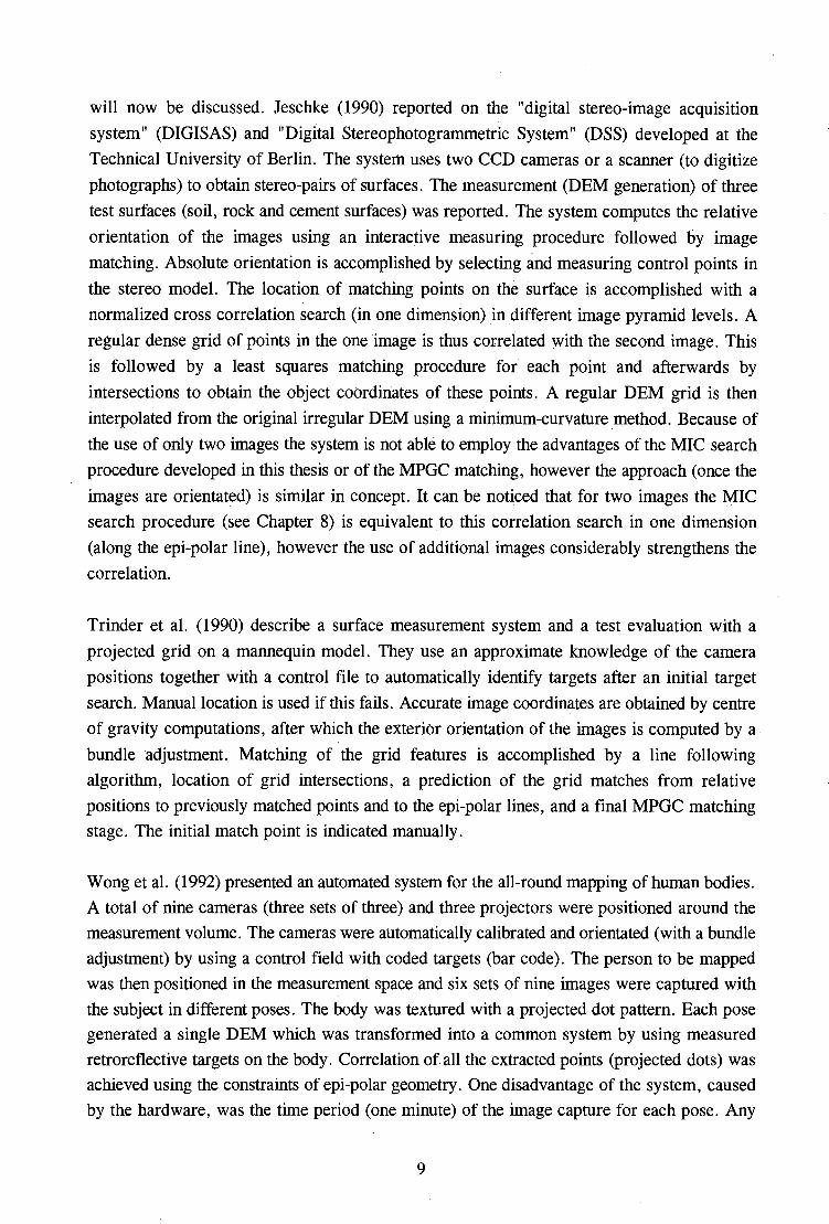
will now be discussed. Jeschke (1990) reported on the "digital stereo-image acquisition

system" (DIGISAS) and "Digital Stereophotogrammetric System" (DSS) developed at the

Technical University of Berlin. The system uses two CCD cameras or a scanner (to digitize

photographs) to obtain stereo-pairs of surfaces. The measurement (DEM generation) of three

test surfaces (soil, rock and cement surfaces) was reported. The system computes the relative

orientation of the images using an interactive measuring procedure followed by image

matching. Absolute orientation is accomplished by selecting and measuring control points in

the stereo model. The location of matching points on the surface is accomplished with a

normalized cross correlation search (in one dimension) in different image pyramid levels. A

regular dense grid of points in the one image is thus correlated with the second image. This

is followed by a least squares matching procedure for each point and afterwards by

intersections to obtain the object coordinates of these points. A regular DEM grid is then

interpolated from the original irregular DEM using a minimum-curvature method. Because of

the use of only two images the system is not able to employ the advantages of the MIC search

procedure developed in this thesis or of the MPGC matching, however the approach (once the

images are orientated) is similar in concept. It can be noticed that for two images the MIC

search procedure (see Chapter 8) is equivalent to this correlation search in one dimension

(along the epi-polar line), however the use of additional images considerably strengthens the

correlation.

Trinder et al. (1990) describe a surface measurement system and a test evaluation with a

projected grid on a mannequin model. They use an approximate knowledge of the camera

positions together with a control file to automatically identify targets after an initial target

search. Manual location is used if this fails. Accurate image coordinates are obtained by centre

of gravity computations, after which the exterior orientation of the images is computed by a

bundle adjustment. Matching of the grid features is accomplished by a line following

algorithm, location of grid intersections, a prediction of the grid matches from relative

positions to previously matched points and to the epi-polar lines, and a final MPGC matching

stage. The initial match point is indicated manually.

Wong et al. (1992) presented an automated system for the all-round mapping of human bodies.

A total of nine cameras (three sets of three) and three projectors were positioned around the

measurement volume. The cameras were automatically calibrated and orientated (with a bundle

adjustment) by using a control field with coded targets (bar code). The person to be mapped

was then positioned in the measurement space and six sets of nine images were captured with

the subject in different poses. The body was textured with a projected dot pattern. Each pose

generated a single DEM which was transformed into a common system by using measured

retroreflective targets on the body. Correlation of all the extracted points (projected dots) was

achieved using the constraints of epi-polar geometry. One disadvantage of the system, caused

by the hardware, was the time period (one minute) of the image capture for each pose. Any

9

small movement by the person during this time would definitely deteriorate the accuracy

achieved.

Another system designed for automated body surface measurements is briefly described by

Mitchell (1994). The system was developed initially for measurement of human backs. Two

cameras and a slide projector (grid pattern) are used, the two images being captured within 0.1

seconds of each other. Detail of the algorithms is not given, except that "least squares image

correlation" is used for reconstructing the surface. However, Mitchell discusses a promising

technique for comparing two surface models which could be used for surface analysis (see

section 9.2).

Test measurements of various surfaces have also been reported by a number of researchers.

These papers often highlight some useful algorithms and techniques which could be

incorporated into a surface measurement system. A few of these will be briefly listed here. For

more information the reader should refer to the quoted papers. Wong and Ho (1986) measured

the one-side of a toy moose without projecting any texture. They gave useful details on

threshold determination for weighted centre of gravity determination, target acceptance

criteria, correlation along epi-polar lines (with some patch shaping) and match point

prediction.

Gruen and Baltsavias (1988) describe the algorithms used for the measurement of a human face

projected with vertical lines. The algorithms include selection of optimal points using an

interest operator, derivation of approximate correspondences and finally MPGC matching. The

correspondence problem is solved by initially finding conjugate lines (determining line pairs

between left and right image) and then determining conjugate points along the lines using the

known camera geometry.

Ruther and Wildschek (1989) report on a projected grid method for reconstructing surfaces.

An initial correspondence for one grid intersection in the images is indicated manually,

whereafter an automatic line tracking procedure and grid intersection detector automatically

and uniquely identifies the remaining grid intersections. This solves the correspondence

problem and thereafter intersections can be performed to determine the 3-D coordinates of the

surface. The algorithm does rely on a continuous grid structure appearing in both images,

which would not be satisfied by all surface types.

Maas (1992b) describes the measurement of a number of different surfaces using projected dots

and an automatic geometric epi-polar matching technique for solving the correspondence

technique. This technique is robust for more than two images and becomes increasingly so as

the number of images increases.

10

Heipke et al. (1994) discuss their algorithms used for measuring a valuable Chinese bronze

vessel. The main technique detailed is the matching procedure. This is accomplished by

"region-growing" matching. An initial known surface match is used as a starting point for

matching close neighbours (With least squares matching), so that the problem of determining

provisional values for conjugate positions of a point is avoided. The process spreads by small

increments until the entire surface is matched. Afterwards the surface coordinates are

computed using intersections. The disadvaptage of this method is that some areas could be left

unmatched if they had big height differences to the surrounding areas, because the provisional

values are being extrapolated as such. However, with many surfaces, the technique can be

expected to work.

Finally, the reader is referred to Wrobel (1991) for a useful review of many surface

reconstruction techniques as well as a description of the "unified least-squares surface

reconstruction" method which matches directly from image space into object surface models.

With many of the systems and techniques described above, the type of projection or targeting

plays an important (if not crucial) part in the design of the algorithms for surface

measurement. Thus, one of the main objectives of this thesis was the development of a suitable

algorithm for determining correspondences between images without any knowledge of the

image structure. This was achieved by the development of the MIC search procedure.

However the algorithm, like most others, does require some surface texture at a point to obtain

a successful result.

11

3. SYSTEM DESIGN

3.1 HARDWARE

The hardware used during the development of the measurement system was comprised of:

(1) commercially available ITC CCD cameras, with specifications as given in table

3.1.

(2) a PIP-512B MATROX framegrabbing card with a 512x512x8-bit frame buffer

size.

(3) a 486 DX-33 personal computer, with an in-built maths co-processor and a

SVGA monitor and graphics card which are needed for image display purposes.

( 4a) an off-the-shelf Enna slide projector for projecting texture onto the surfaces to

be measured. The slides which were used were designed in Harvard Graphics

3. 0 and contained various texture patterns.

(4b) a standard 3M overhead projector for projecting texture. The overheads were

photocopied from Harvard Graphics prints.

A typical hardware configuration is depicted

in figure 3 .1. What could change between

applications is the number and positions of

cameras and the type of texture projected

onto the object surface.

3.1.1 Cameras

The .ITC cameras used are low cost

commercial surveillance cameras. The

limited image format and resolution (see

table 3 .1) determine the relative accuracy

Figure 3.1. Surface measurement equipment and configuration.

that is obtainable. For more precise work, CCD cameras with higher resolution and a larger

image format could be used without altering the system design.

12

\

ITC CCD camera

Sensor type interline transfer

Sensor area 7.95 mm (hz) x 6.45 mm (v)

No. of sensor elements 795 (hz) x 596 (v)

Sensor element spacing 8.6 µm (hz) x 8.3 µm (v)

SIN ratio < 48 dB

Table 3.1. Manufacturer's specifications for the ITC CCD camera.

The relative size of the digitized pixel spacing in the framegrabber of the horizontal and

vertical directions is important to know and this can be computed by including a scale factor

in the one direction as an unknown when calibrating the cameras. The absolute sizes of the two

pixel spacings are not critical because the value . for the principal distance will change

accordingly in order to model the photogrammetric network configuration correctly. It is also

possible to approximately compute their sizes by imaging a plane (containing points of known

coordinates) parallel to the sensor and at a known (fairly large) distance away. In general

however if the manufacturer's specifications for the sensor element spacing and clock

frequency of camera and framegrabber are known then the pixel spacings of the stored image

within the framegrabber can be computed. Due to TV line scanning convention the pixel

spacing in y-direction is identical to the sensor element spacing in y-direction (Lenz and

Fritsch, 1990). The pixel spacing in x-direction can be determined from the sensor element

spacing by using the following equation:

in which:

ps x

~ =SS -Xf

p

picture element (pixel) spacing in x (in framegrabber),

sensor element spacing in x,

pixel clock frequency of the camera and

clock frequency of the framegrabber.

13

(3.1)

3.1.2 Framegrabber

The PIP-512B framegrabber is only capable of capturing one 512x512 image at a time (30

images per second). This is acceptable for static objects. If moving objects are to be measured,

a framegrabber which is capable of simultaneously capturing multiple images is needed. If

higher resolution cameras are incorporated within the system then a suitable framegrabber with

larger storage is required. No framegrabbing card is required in the case of fully digital

cameras where the digitization already occurs in the camera.

3.1.3 Computer

The software has been designed to run under DOS on personal computers with a 386 or higher

processor, but the system design and algorithms would remain the same on other platforms

(such as Unix based workstations). The only changes would occur with the interface and

graphics routines. Currently personal computers are in a stage where their performance is

rapidly improving, thus a measurement system such as this one can significantly increase its

processing speed by replacing the present computer with a later version.

3.1.4 Projectors

Any slide or overhead projector which can guarantee slide and projection stability can be used

for the projection of texture onto the objects surfaces. The Enna slide projector and the

overhead projector used for this work were tested for stability by performing repeatability tests

on a projected dot pattern.

Forty images were captured for both projection devices. The first ten images were captured

in the first ten seconds of projection, the second ten in the next thirty seconds, the third ten

in the following ninety seconds and the last ten in a final ten minutes. The weighted centre of

gravity with grey value squared as weight was used for the centering of all the projected dots

(over one hundred dots for each device) in all the images. The results for both devices are

shown in tables 3.2 and 3.3.

14

.• .•

Repeatability test for slide projector pattern. (units: pixels)

Images compared RMSVX RMS Vy MaxVx MaxVv

1,2, ... ,10 0.044 0.058 0.187 0.194

11,12, ... ,20 0.073 0.074 0.188 0.176

21,22, ... ,30 0.033 0.037 0.116 0.112

31,32, ... ,40 0.046 0.267 0.156 0.632

1,2, ... ,40 0.239 0.353 0.518 0.956

1,10 0.071 0.094 0.142 0.165

11,20 0.114 0.118 0.163 . 0.150

21,30 0.046 0.024 0.077 0.055

31,40 0.074 0.419 0.124 0.479

1,40. 0.361 0.317 0.452 0.416

Table 3.2. Results of repeatability test of slide projector pattern starting from switch-on.

Repeatability test for overhead projector pattern. (units: pixels)

Images compared RMSVX RMS VY MaxVx MaxVv

1,2, ... ,10 0.019 0.020 0.090 0.117

11,12, ... ,20 0.024 0.021 0.094 0.136

21,22, ... ,30 0.023 0.022 0.103 0.112

31,32, ... ,40 0.031 0.034 0.312 0.242

1,2, ... ,40 0.057 0.038 0.483 0.386

1,10 0.022 0.017 0.071 0.059

11,20 0.030 0.018 0.078 0.056

21,30 0.026 0.014 0.060 0.055

31,40 0.036 0.042 0.236 0.181

1,40 0.092 0.066 0.291 0.256

Table 3.3. Results of repeatability test of overhead projector pattern starting from

switch-on.

15

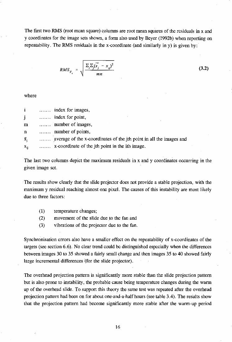
The first two RMS (root mean square) columns are root mean squares of the residuals in x·and

y coordinates for the image sets shown, a form also used by Beyer (1992b) when reporting on

repeatability. The RMS residuals in the x-coordinate (and similarly in y) is given by:

where

J

RMSV r

index for images,

index for point,

number of images,

number of points,

mn

average of the x-coordinates of thejth point in all the images and

x-coordinate of the jth point in the ith image.

(3.2)

The last two columns depict the maximum residuals in x and y coordinates occurring in the

given image set.

The results show clearly that the slide projector does not provide a stable projection, with the

maximum y residual reaching almost one pixel. The causes of this instability are most likely

due to three factors:

( 1) temperature changes;

(2) movement of the slide due to the fan and

(3) vibrations of the projector due to the fan.

Synchronisation.errors also have a smaller effect on the repeatability of x-coordinates of the

targets (see section 6.6). No clear trend could be distinguished especially when the differences

between images 30 to 35 showed a fairly small change and then images 35 to 40 showed fairly

large incremental differences (for the slide projector).

The overhead projection pattern is significantly more stable than the slide projection pattern

but is also prone to instability, the probable cause being temperature changes during the warm

up of the overhead slide. To support this theory the same test was repeated after the overhead

projection pattern had been on for about one-and-a-half hours (see table 3 .4). The results show

that the projection pattern had become significantly more stable after the warm-up period

16

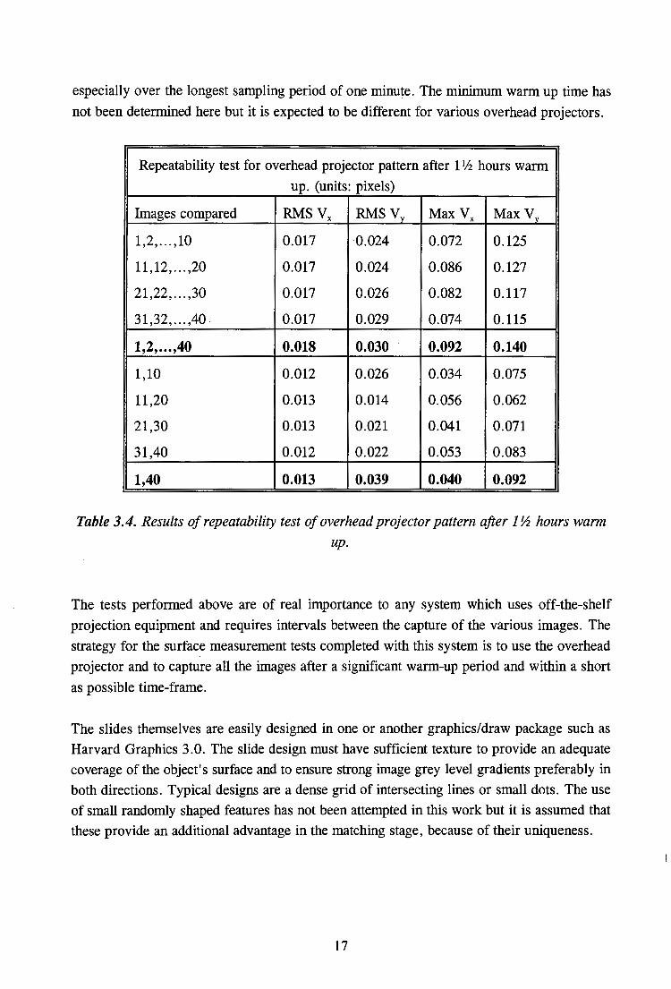
especially over the longest sampling period of one minute. The minimum warm up time has

not been determined here but it is expected to be different for various overhead projectors.

Repeatability test for overhead projector pattern after l 1h hours warm

up. (units: pixels)

Images compared RMSVX RMS VY MaxVx MaxVv

1,2, ... ,10 0.017 0.024 0.072 0.125

11,12,. . .,20 0.017 0.024 0.086 0.127

21,22, ... ,30 0.017 0.026 0.082 0.117

31,32,. . .,40 0.017 0.029 0.074 0.115

1,2, ... ,40 0.018 0.030 0.092 0.140

1,10 0.012 0.026 0.034 0.075

11,20 0.013 0.014 0.056 0.062

21,30 0.013 0.021 0.041 0.071

31,40 0.012 0.022 0.053 0.083

1,40 0.013 0.039 0.040 0.092

Table 3.4. Results of repeatability test of overhead projector pattern after 1 Y2 hours warm up.

The tests performed above are of real importance to any system which uses off-the-shelf

projection equipment and requires intervals between the capture of the various images. The

strategy for the surface measurement tests completed with this system is to use the overhead

projector and to capture all the images after a significant warm-up period and within a short

as possible time-frame.

The slides themselves are easily designed in one or another graphics/draw package such as

Harvard Graphics 3.0. The slide design must have sufficient texture to provide an adequate

coverage of the object's surface and to ensure strong image grey level gradients preferably in

both directions. Typical designs are a dense grid of intersecting lines or small dots. The use

of small randomly shaped features has not been attempted in this work but it is assumed that

these provide an additional advantage in the matching stage, because of their uniqueness.

17

3.2 SOFTWARE

A substantial amount of software was developed as part of the work for this thesis, specifically

for the measurement system and also for additional programs which analysed test results and

performed many other related functions. Various C compilers including Microsoft Quick C

(version 2.0), Borland C (version 3.0) and Gnu C (version 1.11) have been used for compiling

the various programs. However, for the final measurement system program the Gnu C

compiler was utilised because of its 32-bit DOS extender allowing the user to directly allocate

all available extended memory (up to 128 Mbytes of RAM) and' also 128 Mbytes of disk space

(if required). The Gnu C compiled executable is significantly faster than the Microsoft and

Borland compiled versions because of the 32-bit processing. As an example a bundle

adjustment executed with the Gnu C version was approximately 2.5 times faster than the

Borland C executable. The extended memory allocation feature allows multiple images to be

simultaneously resident in memory, as opposed to the 640 Kbytes DOS limit associated with

the other conventional compilers.

The software has a project orientated design, and results, both at intermediate and final stages,

are stored in project files. For example, this allows the user to try different centering

techniques without having to extract and compute provisional image coordinates of the targets

again.

3.3 THE MEASUREMENT PROCEDURE

The measurement procedure can be divided. into two different cases. The first case is adopted

when the exterior orientation of the cameras is unknown and needs to be computed. This

occurs in cases of once-off measurements (see figure 3.3) or with an initial orientation for on­

lihe or dedicated camera set-ups. Ideally the camera calibration is performed before each

surface measurement (in once-off tasks), but this might be unnecessary with more stable

cameras which are carefully handled.

The other case is used with camera configurations of known exterior orientation, such as

occurs with dedicated systems (see figure 3.2). This type of system would theoretically require

one orientation procedure because of the set positions of the cameras, however in practise the

orientations would be automatically updated whenever changes were detected (see Chapter 7).

One could perform a once-off pre-calibration of the cameras in a stable environment, however,

repeated calibrations may become necessary in less stable surroundings, including areas with

vibrations or big temperature changes, which might affect the internal stability of the camera

body, lens and sensor over time.

18

In both cases the main algorithms can remain exactly the same, just the execution sequence

will change and the dedicated set-up would have an additional routine for automatic update

orientation.

Free Network Camera Calibration

,,.

Exterior Orientation , ....

Determination

,.,

. Surface Measurement

No Yes ,.,

Update orientation?

Figure 3.2. The measurem_ent procedure for a dedicated set-up.

Free Network Camera Calibration

,,.

Exterior Orientation Determination

,.,

Surface Measurement

Figure 3.3. The once-off measurement procedure.

For the rest of this thesis a once-off measurement procedure is assumed, except in the

discussions of Chapter 7, which describe these cases in more detail.

The procedures for both the camera calibration and exterior orientation are identical except for

the parameters used in the bundle adjustment. In the calibrati.on stage, all parameters (inner·

orientation, additional and exterior orientation parameters) are included as unknowns while in

. the exterior orientation stage the Inner orientation and additional parameters are held fixed

(known quantities) and. only the exterior orientation parameters are solved for. The process for

these two tasks (calibration and orientation) is described with the flowchart in figure 3.4.

19

Image capture Extract point

1 of interest

Extract control targets '"

1 Locate conjugate

Accurate target point in all images (rough matching).

centering

1 Target .i.

MPGC (fine) identification

1 matching

Calibration or orientation using

bundle adjustment Update DEM

Figure 3.4. The various stages required for Figure 3.5: The measurement procedure for a calibrating and/or orientating the camera(s). single point on the surface.

Figure 3.5 depicts the measurement process for a single point on the surface being measured.

Each extracted point is processed this way until the routine finds no more interest points. Each

of the stages shown in both these figures are described in more detail in the ensuing chapters,

however they have been presented here to demonstrate the system design and the interaction

of the various algorithms.

20

4. SYSTEM CALIBRATION

A thorough system calibration, whether self-calibration or pre-calibration is crucial to

obtaining good, reliable three dimensional coordinates of points in space. Sources of

significant radiometric and geometric errors should be identified and their effects minimised

by careful hardware preparation and adequate modelling of distortions. Before discussing the

properties of cameras and framegrabbers affecting the images, a brief description of the image

coordinate system and of the collinearity equations is given.

Images are stored as arrays of intensity values (0 to 255 for 8-bit images). Thus the pixel

coordinate system is defined by the subscripts of the array as shown in figure 4 .1, with the

centre of the first pixel having pixel coordinates of (0,0).

Pixel coordinate Image coordinate

system system

y

x

Image - . x

Image

y

Figure 4.1. Definition of the pixel and image coordinate systems.

The conventional image coordinate system (from film-based photogrammetry) usually has its

origin at the intersection of the fiducial marks (approximately at the c.entre of the image), the

direction of its positive y-axis opposite to the y-axis of the pixel coordinate system and it has

units of millimetres. The transformation from pixel to image coordinate system can thus be

given by the following two equations:

21

in which

Xpix• Ypix

nx, ny

PSx, psy

x. 1mg

Y;mg

n. - 1 - x

) psx = (x pix

2

n - 1 = (

y

2 - Yp) psy

pixel coordinates of a point,

number of pixels in x and y directions,

pixel spacings in x and y directions and

image coordinates of the point.

(4.1)

(4.2)

The transformations given by equations 4.1 and 4.2 involve a shift of the origin from the top

left pixel in the image to the centre of the image, a reflection of the y-axis and a scale change

in both directions.

The perspective transformation from a point,.in space.(X,Y,Z), through a camera lens system,

to a point on' the image plane (x,y) in the image coordinate system is given by the collinearity

equations:

+ dxd x - x p

y - Yp + dyd

where

x,y

xP, Yp

dxd, dyd

c

rij

Xe, Ye, Ze X, Y,Z

~~~ ___ :__' ----·-----"-------'---

= c

= c

r11

(X-X) +r (Y-Y) 12 c + r (Z-Z) 13. c

r31(X-X) +r (Y-Y) 32 c + r (Z-Z) 33 c

r21(X-X) +r (Y-Y) 22 c + r (Z-Z) 23' c

r3l(X-Xc) +r (Y-Y) 32 c + r (Z-Z) 33 ·, c

image coordinates of a point~

principal point coordinates,

distortion corrections,

principal distance,

elemen.ts of a 3x3 orthogonal rotation matrix, R,

perspective centre coordinates and

space coordinates of the point.

22

(4.3)

(4.4)

Equations 4.3 and 4.4 are modified collinearity equations as the distortion corrections, dxd and

dyd, allow for deviations from the ideal co1linearity and co-planarity assumptions. The

principal distance or camera constant, c, is the perpendicular distance.between the image plane

and the perspective centre (interior). The principal point is defined by the intersection of this

perpendicular line with the image plane. The nine elements of the orthogonal rotation matrix

are functions of the three rotations about the X, Y and Z axes. In analytical photogrammetric

solutions any rotation sequence can be adopted to form the full rotation matrix (Tµompson,

1969).

4.1 GEOMETRIC DISTORTIONS AND RADIOMETRIC PROPERTIES OF A

CAMERA-FRAMEGRABBER SYSTEM

4.1.1 Geometric Distortions

A number of distortion models have been investigated and implemented in photogrammetric

measurement applications over the years to correct for known physical distortions of image

coordinates. The fairly recent use of CCD cameras, which have some different properties and

thus different deformations to film-based cameras, has added to the research into proper

modelling of significant geometric distortions. Some sources of error, such as lens distortion,

have still remained the same. The following sections discuss potential sources of geometric

errors.

4.1.1.1 Lens distortion

Two types of image distortions caused by the lens system in a camera are usually modelled,

namely radial distortion and decentering distortion. Radial distortion is a phenomena apparent

in all lenses. The distortion increases with smaller focal lengths, thus it is extremely important

to model it in dose-range applications. Radial distortion may be slightly asymmetric, but it is

conventionally shown as symmetric about a "principal.point of best symmetry" (Fryer, 1989)

which does not necessarily coincide with the principal point. This point is the intersection of

the optical axis of the lens with the sensor surface. According to Burner et al (1990)

misalignment angles of up to 0.5 degrees have been found for several solid-state cameras. This

misalignment angle is the angle at the perspective centre between the optical axis direction and

the direction.to th~ principal point. However, this "principal point of best symmetry" is usually

considered coincident with the principal point for computations of lens distortion parameters.

23

Decentering distortion·occurs due to the misalignment of the lens components. In a perfect lens

system the centres of curvatures of all the spherical surfaces are collinear with the optical axis.

Decentering distortion is comprised of both a tangential and a radial component.

Lens distortions can be modelled with the following equations (Brown, 1971):

in which

-y

image distortion of a point in the x coordinate direction.

image distortion of a point in the y coordinate direetion.

x image coordinate of a point reduced to the principal point

(equal to x - xp).

y image coordinate of a point reduced to the principal point

(equal toy - yp).

(4.5)

(4.6)

is the radial image distance between the point and the principal point.

radial lens distortion parameters

decentering lens distortion parameters

The distortion parameters are only valid for points on the plane of focus, so if big depths of

field are encountered, the corrections applied to a point should theoretically take the distance

of the point from the camera.into account (see Fryer and Brown, 1986). In this case the lens

distortion parameters need to be calibrated- for two different focus settings to accurately

compute the correct adjustment at a point (Fryer, 1989). It is thus important that a calibrated

camera should be used at approximately the same distance at which it was calibrated, if no

extra modelling of the effect of object distance on the I.ens distortion parameters is employed.

4.1.1.2 Image plane unflatness

The collinearity equations are based on two basic assumptions. The first is that an object point,

its image point and the perspective centre are collinear, and the second is that all image points

lie in a plane. Lens distortions cause non-collinearity and these can be easily modelled.

Unflatness of the image "plane" cause radial distortions of image points.

24

Polynomials describing the deviations of the image surface from a true plane can be computed

(see Brown, 1980) and then corrections applied to any resulting image coordinates. Of

particular importance is the fact that errors induced by unflatness are not significantly revealed

by the standard deviations of the 3-D object coordinates or by the residuals of the image

coordinates, but they tend to cause errors in the resulting 3-D object coordinates (Brown,

1980). Thus it is important to know the flatness of any imaging device. The radial correction

(or) needed to compensate for an unflatness, oh (distance from the ideal image plane), at an

image point is (from Brown, 1980):

Or = Oh--r­c - oh (4.7)

in which c is the principal distance of the camera and r is the radial distance from the principal

point to the image point in question.

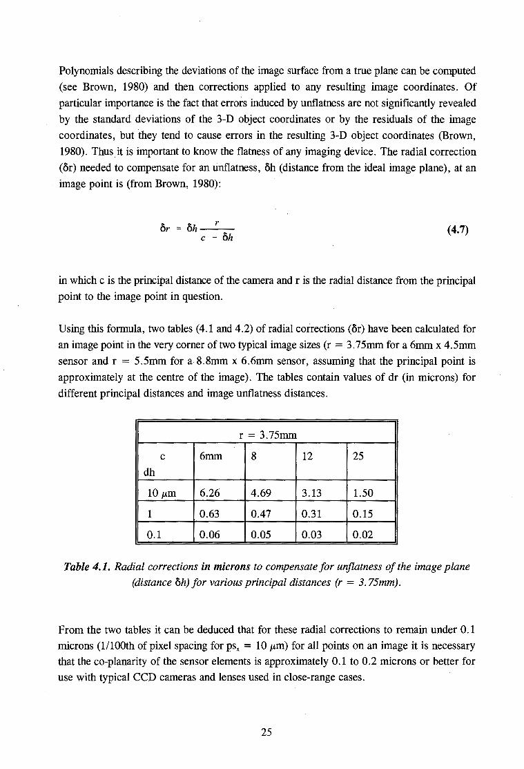
Using this formula, two tables (4.1 and 4.2) of radial corrections (or) have been calculated for

an image point in the very comer of two typical image sizes (r = 3.75mm for a 6mm x 4.5mm

sensor and r = 5.5mm for a 8.8mm x 6.6mm sensor, assuming that the principal point is

approximately at the centre of the image). The tables contain values of dr (in microns) for

different principal distances and image unflatness distances.

r = 3.75mm

c 6mm 8 12 25

dh

10 µm 6.26 4.69 3.13 1.50

1 0.63 0.47 0.31 0.15

0.1 0.06 0.05 0.03 0.02

Table 4.1. Radial corrections in microns to compensate for unflatness of the image plane

(distance oh) for various principal distances (r = 3. 75mm).

From the two tables it can be deduced that for these radial corrections to remain under 0.1

microns (1/lOOth of pixel spacing for psx = 10 µm) for all points on an image it is necessary

that the co-planarity of the sensor elements is approximately 0 .1 to 0. 2 microns or better for

use with typical CCD cameras and lenses used in close-range cases.

25

r = 5.5mm

c 6mm 8 12 25

dh

10 µm 9.18 6.88 4.59 2.20

1 0.92 0.69 0.46 0.22

0.1 0.09 0.07 0.05 0.02

Table 4.2. Radial corrections in microns to compensate for unflatness of the image plane

(distance oh) for various principal distances (r = 5.5mm).

According to Haggren (1989) the deviations in flatness typically remain below· 1/lOOth of the

sensor element spacing, however he does not mention the size of the sensor element spacing.

Assuming a size of less than 20µm this high geometrical consistency would meet the

requirements of most systems. However, Beyer (1992b) writes that the surface topography

variation (from a plane) can reach several microns. Looking at the two tables above, this size

of unflatness would have a significant effect. It seems that further investigations of variations

of the sensor surface need to be carried out to obtain a clearer insight into their size and scope.

If the sensor flatness can be measured, or is known from the manufacturer's specifications,

then equation 4.7 or the tables 4.1 and 4.2 can be used to see whether any significant

distortions caused by image unflatness could arise.

4.1.1.3 Regularity of the sensor element spacing

CCD sensors generally exhibit extremely high regularity df the sensor element spacing. Lenz

(1989) used interferometry to show 'that the regularity was about 0.1 micron which was

equivalent to just less than 1/100 th of the sensor element spacing. This high regularity can be

degraded by the framegrabber if PLL synchronization is used (see section 4.1.1.5).

4.1.1.4 Orthogonality of the sensor axes

In a perfect sensor, the two sensor axes are exactly at 90 degrees to each other. Due to

manufacturing imprecisions the axes can become non-orthogonal. Burner et al (1990)

investigated six CCD cameras and two CID cameras and found that the two CID cameras had

26

significant angles of non-perpendicularity, with differences in the order of 0.1 degrees from

the manufacturer's specifications. Distortion corrections for affinity and lack of orthogonality

of the image coordinate system can be written as:

(4.8)

- -dy d = b21x + b22Y (4.9)

in which the "b" terms are parameters describing the image distortion due to affinity and lack

of orthogonality.

4.1.1.5 Line jitter and PLL synchronization

Line-jitter is a horizontal displacement between lines (rows) in an image and is caused by

imperfect synchronisation between camera and framegrabber. According to Lenz and Fritsch

(1990) most line-jitter erro!s are due to the loss of perfect synchronisation during the vertical

blanking period, while much less occur from the phase-locked-loop (PLL) control oscillations.

Not only does line-jitter occur between lines in an image but it can change with the location

along the line (Beyer, 1987) due to PLL synchronization. Line jitter is eliminated when using

a pixel-clock for synchronization or when using digital cameras.

A simple test was performed to determine the extent of the random line-jitter errors induced

by the PLL synchronisation associated with the ITC camera and the PIP-512B Matrox

framegrabber. A sheet of white paper with a thick black vertical stripe was imaged

sequentially, resulting in ten images captured over approximately 11 seconds. For this purpose

the software selectable offset and gain were adjusted so that the range of grey values fell

between 30 and 230 and the cameras had been warmed up for a number of hours to avoid

warm-up effects (see for example Dahler, 1987). The vertical black and white edge covered

all the rows in the images. No assumption about the edge being a straight line was made, the

objective was to determine the repeatability of each row's sub-pixel edge position in the ten

images. The repeatability of the edge position in x-direction was determined using the same

formula as equation 3. 2 in chapter 3 except that the subscript j refers to the row and not to the

point.

The sub-pixel positions of the edges in each row and each image was computed using the

moment preserving method (Tabatabai and Mitchell, 1984), described in more detail in section

27

6.3. RMSx is the root mean square of the residuals for each row. The result of this test are

depicted in table 4.3 below.

RMS V x (pels) Max. residual (pels)

0.027 0.128

Table 4.3. Results of line-jitter test.

Looking at the maximum residual shows that the random component of line-jitter is significant.

Computing centres of targets which are a number of pixels in extent reduces the effects of

random line-jitter in most cases, as does using image patches when matching, however errors

in the x-direction still remain. Averaging of images can help reduce this phenomena.

Beyer (1992b) lists a number of effects caused by PLL synchronisation, these are:

(1) shear of imagery,

(2) line-jitter of typically larger than 0.1 pixel,

(3) scaling in the x-direction and aliasing effects,

( 4) changing scale within each line and

(5) phase patterns.

To compensate for the shear and the scaling in the x-direction, Beyer uses the following

distortion corrections:

dxd = xsx + ya (4.10)

(4.11)

in which sx is the parameter correcting the scaling in the x-direction and 'a' is the parameter

correcting for shear of the imagery (in the horizontal direction). The scale factor in the x­

direction, sx, will also correct for an imprecise pixel spacing value. To eliminate the other

effects pixel-synchronous sampling or cameras with digital output should be used.

28

4.1.1.6 Other sources of error

Various systematic errors can be accounted for by further modelling using a number of

approaches. Grun (1978) developed a large orthogonal polynomial set of additional parameters

with respect to a 5 x 5 image grid for modelling arbitrary deformations, although sophisticated

statistical testing of the parameters' significances was needed to avoid high correlations and

overparameterization.

Amdal et al (1990) use B-Spline surfaces to model remaining local systematic distortions in.

both x and y directions, after correcting for affinity and lack of orthogonality of the image

coordinate system as well as radial and decentering lens distortfon.

Another error, known as centering error, which is caused by the obliqueness of targets with

respect to the image plane is discussed in chapter 5.

The full distortion model incorporated as part of the bundle adjustment and for all the system

measurement tasks in this work included three radial and two decentering lens distortion

parameters, a scale factor in the x-direction and an image shear, and was given by:

(4.12)

(4.13)

in which the variables have the same meaning as in equations 4.5, 4.6, 4.10 and 4.11. This

parameter set has been used by Beyer (1992a and 1992b) in a 3-D test field network using PLL

synchronisation.

4.1.2 Radiometric Properties

The radiometric properties of cameras and framegrabbers affect the image quality which in

turn can have an effect on the positional accuracy obtainable. However, in all the practical

work carried out for this project no radiometric calibration of the system was performed. Basic

adjustments to the offset and gain were applied and the cameras were always warmed up for

a number of hours. The multiphoto geometrically constrained matching model automatically

does compensate for additive and multiplicative radiometric differences between the images,

but further modelling of other sources of radiometric errors was not performed.

29

Radiometric properties of camera and framegrabber systems have been investigated by Lenz

and Fritsch (1990), Beyer (1994), Raynor and Seitz (1990), Dahler (1987) and others.

Van den Heuvel (1993) gives an account of a radiometric calibration and how it affected the

resulting space precisions. Dark signal non-uniformity and photo-response non-uniformity

were corrected for resulting in a 2 % improvement in the variance factor of the bundle adjustment.

4.2 FREE NETWORK BUNDLE ADJUSTMENT

To obtain the observation equations for a least squares bundle adjustment, the collinearity

equations 4.3 and 4.4 need to be linearised through a Taylor's series expansion. The entire set

of observation equations is in the usual parametric least squares form:

v =Ax - I (4.14)

and the corrections to the parameters can be computed from

(4.15)

in which N is the normal equation matrix given by

(4.16)

and

c =A rpz (4.17)

where P is the weight matrix.

The programmed bundle adjustment has been flexibly designed for various types of networks

and measurement tasks. It can process either resections, intersections or both. The interior

orientation parameters and additional parameters (both referred to here as camera parameters)

can be block invariant or variant or a combination of both; each image can be linked to any

set of camera parameters. In addition the bundle adjustment can be processed as a constrained

30

network or as a free network. Geodetic distance obs~rvations can be input as part of the

adjustment, providing a useful way of scaling a free. network.

There is also an option to input a priori standard deviations and correlations for the

observations (x and y image coordinates). By default the observations are treated as equally

precise and uncorrelated. The observations can either be in the pixel coordinate system or the

image coordinate system or a combination of both. Any mixture of camera parameters or

exterior orientation parameters (referred to here as station parameters) can be held fixed

(known and not solved for) or free {unknown and solved for). A partitioning solution (see

section 4.2.1) allows many images and points to be processed simultaneously, the practical

limit only being imposed by the amount of free RAM on the computer. With the Gnu C

compiled program the processor will automatically swap to disk if required, but this would

considerably slow down the processing time.

The bundle adjustment program also has a comprehensive· result file which includes amongst

other things the:

(1) network information (number of observations, images, cameras, etc.),

(2) degrees of freedom,

(3) a posteriori standard deviations of unit weight, a0 ,

( 4) a chi squar~d test of the a priori and a posteriori standard deviations of unit

weight (if a priori standard deviations and correlations of the observations are

input),

(5) all computed parameter values and their standard deviations,

(6) correlations between the camera parameters for every camera, and between the

camera parameters and the ~tation parameters for every station,

(7) observations (image coordinates), their distortion corrections and their residuals

and

(8) a list of observations which fail an outlier detection test (observations with a

residual greater than three times the a0).

4.2.1 Partitioning of the Normal Equation System

In order to conserve memory space and to speed up the adjustment procedure, the normal

equations can be partitioned to exploit the inherent sparsity of the normal equation matrix.

31

The entire set of norma:I equations is given by:

Nx = c (4.18)

The free network approach of inner constraints is used to implicitly define a datum (Fraser,

1987). This allows the shape of the network to be solved for, while the position, orientation

and scale are defined by the provisional values of the parameters. A free network solution can

be obtained through the inner constraints simply by bordering the singular normal equation

matrix N with a transformation matrix G which satisfies the condition AG = 0 (Fraser, 1982).

It is important to note that there are a number of other mathematically equivalent techniques

to obtain an inner constraint solution. Now, adding the inner constraints to equation 4.18

gives:

(4.19)

in which lambda is a vector of Lagrangian multipliers. If we now partition N with respect to

camera parameters (subscript c), station parameters (subscript s), points involved with

distance observations (subscript d) and other points (subscript p) we can expand equation 4.19

into equation 4.20 below. As before, camera parameters are defined here as inner orientation

parameters and additional parameters while station parameters are defined as the elements of

exterior orientation.

N N Ned N G c cs cp c x cc c

T N Nsd N G Ncs ·s sp s x cs s

T T Nd Ndp Gd (4.20) Ned Nsd xd = Cd

T T T N G x c Ncp Nsp Ndp p p p p

GT GT GT GT 0 A. 0 c s d p

Re-arranging the order of parameters (moving points to the end) gives:

32

N N Ned G N c cs c cp Xe c c

T N Nsd G N Ncs s s sp x c s s

T T Nd Gd Ndp (4.21) Ned Nsd xd = Cd

GT GT GT 0 GT A. 0 c s d p

T T T x c Ncp Nsp Ndp G N

p p p p

Imposing inner constraints on only the point parameters (applying· partial inner constraints)

results in a minimum standard deviation for the point parameters (see Fraser, 1982). Thus, in

this case Ge = 0 and Q = 0. Additionally it can be easily noticed that if there are no

correlations between the points with geodetic distances and the other points then Ndp = 0,

which is the usual assumption in photogrammetric solutions. This same assumption leads to

the matrix NP having a diagonal structure of 3x3 sub-matrices pertaining to each point. The

normal equation system can now be re-written as:

N N Ned 0 N c cs cp x c c c

T N Nsd 0 N Ncs s sp x c s s

T T Nd Gd 0 (4.22) Ned Nsd xd Cd

0 0 GT 0 GT A. 0 d p

T T x c Ncp Nsp 0 G N

p p p p

or

(4.23)

where

(4.24)

33

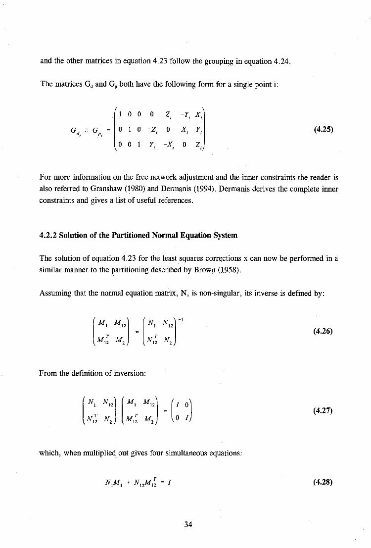
and the other matrices in equation 4.23 follow the grouping in equation 4.24.

The matrices Gd and GP both have the following form for a single point i:

1 0 0 0 Z. -1. x. I I /,

Gd - G = 0 1 0 -Z. 0 x. y (4.25) P; I I I

I

0 0 1 y -X. 0 Z. I I I

For more information on the free network adjustment and the inner constraints the reader is

also referred to Granshaw (1980) and Dermanis (1994). Dermanis derives the complete inner

constraints and gives a list of useful references.

4.2.2 Solution of the Partitioned Normal Equation System

The solution of equation 4.23 for the least squares corrections x can now be performed in a

similar manner to the partitioning described by Brown (1958).

Assuming that the normal equation matrix, N, is non-singular, its inverse is defined by:

(4.26)

From the definition of inversion:

(4.27)

which, when multiplied out gives four simultaneous equations:

(4.28)

34

(4.29)

(4.30)

(4.31)

Solving for M12T in equation 4.30 gives:

(4.32)

Substituting equation 4.32 into equations 4.28 and 4.31 yields:

(4.33)

(4.34)

from which exptessions for M1 and M2 can be obtained:

(4.35)

(4.36)

Equations 4.35, 4.36 and 4.32 can be used to compute the normal equation matrix inverse. . .

The least squares parameter corrections are calculated from:

(4.37)

35

or

(4.38)

(4.39)

Other properties of the normal equation matrix can be used to further increase the efficiency

of this solution. It is possible to determine suitable provisional values for the points without

. associated geodetic distance equations so that the vector c2 reduces to zero. This can be

achieved by assuming the x1 parameters (see equation 4.23) are known and solving the reduced

system:

(4.40)

or

(4.41)

By solving equation 4.41 iteratively for x2 , the c2 reduces to zero. Because of the diagonality

of the matrix N2, given by:

Nz 0 0 I

0 Nz 0 2

Nz (4.42)

0 0 Nz np

in which "np" is the number of points without distance observations, each of the x2i are solved

for using:

(4.43)

36

Thus , every point i (without distance observations) is processed so that it obtains new

coordinates which results in c2i reducing to zero. Once all these points are similarly processed,

Ci is reduced to zero and equations 4.38 and 4.39 become:

(4.44)

(4.45)

Some other properties of the partitioned normal equation matrix were used to further simplify

the solution of the normal equation system, however the reader is referred again to Brown

(1958) for the full solution. The slightly different partitioning employed here for the free

network and the distance observations can be used with the same method.

4.3. CONTROL FIELD

A well designed control field is one of the requirements for accurate camera calibration.

Torlegard (1981) outlines the multi-concept for improving accuracy in all types of

photogrammetric networks . The multi-concept includes the use of multiple stations, multiple

images at a station and multiple control (object) points. Thus a large number of well

distributed points is the basic requirement for a control field. A control field , see figure 4.2,

was designed for the dual purpose of camera

calibration and as control for the

measurement of objects .

The frame's size was 60x60cm of which the

targets covered an area of 50x50cm. To

provide depth in the field eight 1 Ocm high

rods and sixteen 20cm high rods were

symmetrically positioned towards the outside

of the frame leaving a 30x30cm area within

the middle to position objects for

measurement. The rods were bolted onto the

6mm steel plate. The control frame was

stable but also very heavy . Circular Figure 4.2. The control field used for camera calibration and exterior orientation.

37

retroreflective targets of 8m.m diameter were placed on the rods and on the plate giving a total

of 101 control points .

Due to the fact that the free network approach is adopted for camera calibration the control

field was not pre-surveyed as such. However, as a check and to provide scale, thirteen of the

targets on the frame were coordinated using theodolite observations from three fixed pillars .

The X and Z (plane) coordinates were determined by a least squares intersection to precisions

of 0.08m.m in X and 0.30m.m in Z (depth) . The Y coordinates (heights) were then computed

using these X and Z coordinates and the vertical angles from the three pillars. The average of

the three resulting Y coordinates was taken and the RMS of the standard deviations of the

mean was 0 .1 lmm. The longest distance between two of these targets in the X-direction was

used to provide scale for the free network adjustments.

As an example of a camera calibration and to accurately coordinate the targets, a set of

fourteen images of the control field was acquired. Five images were taken with a ninety degree

roll about the camera axis. All ten additional parameters were included as unknowns in the free

network adjustment, and the single distance observation was given a small a priori standard

deviation to provide the scale. An initial adjustment produced 16 observation outliers . These

were investigated on the images and every one of them was found to be a partially occluded

target, thus clearly demonstrating the good inner reliability of the network. Only a further two

partially occluded targets were not identified as outliers, however these were picked up as new

outliers in the next adjustment. A summary of the final results is shown in table 4.4 with and

without the full additional parameter set.

Version df ao RMS (mm)

ax Oy Oz vx Vy

No AP's 2283 0.0020 0.092 0.106 0.315 0.0019 0.0018

7 AP's 2276 0.0003 0.014 0.016 0.046 0.0003 0.0002

Improvement factor 6 .7 6.6 6.6 6.8 6.3 9.0

Table 4.4. Results of a free network adjustment without additional parameters and with the

seven additional parameters. The improvement factor is shown.

The results clearly show the improvements in the precision and size of residuals when

distortions are modelled by additional parameters. As can be seen from the results a

relative accuracy of about 1 :35000 in the X direction and 1 :30000 in the Y direction has

38

been achieved in object space with the 512x512 imaging resolution. In image space the

RMS of the residuals is equivalent to about l/40th of the pixel spacing in x (taken as 11 .83

micron) and l/40th of psy (taken as 8.35 micron).

As a matter of interest the 13 points coordinated by theodolite were transformed by means

of a least squares 3-D transformation into their photogrammetric coordinates. The RMS of

the resulting residuals in X,Y and Z was 0.08mm, 0.09mm and 0.15mm respectively.

These figures show that the two sets of coordinates agree well with each other.

One of the disadvantages of this specific

control field was that the rods tended to

occlude quite a few of the outer targets on

the plate. A second control frame, see

figure 4. 3, more in the shape of a box has

thus been used for the calibration of

cameras. This frame structure was lighter

but no less stable than the previous one.

The frame had 90 targets at two different

depths with a target layout design to

produce fewer occlusions. In addition, the

centering of targets on narrow rods and

bars can be adversely affected by the

proximity of these strong physical edges.

Both these problems can be solved by the

control field design described in Beyer

Figure 4.3. The second control frame used for camera calibration.

(1987) in which a single plane of targets on an aluminium plate is moved by a sledge

system with rotary encoders to a precision of approximately 10 microns. Images are taken

with the plate at different depth positions. The disadvantages of such a system are the

difficulty and expense of production as well as the dependence of the repeatability of the

target positions on the accuracy of the encoders. However, this repeatability is only needed

if a constraint network is required or if some of the target positions are used as check

points.

4.4 CONCLUSIONS OF CHAPTER

Modelling of geometric camera distortions is a prerequisite for medium or high accuracy

measurements. The specific calibration reported on in this chapter showed almost a seven

times improvement in precision when using the chosen additional parameter set over the

version without additional parameters.

39

The free network is a flexible way of solving a photogrammetric network when no accurate

control exists. Scale can be provided by one or more distance observations. Imposing inner

constraints on only the object point parameters results in a minimum variance for the object

coordinates.

Camera pre-calibration to compute the camera parameters is advisable for dedicated set-ups

using different cameras. In other cases the use of a self-calibrating network adjustment is

preferable. Pre-calibration has the disadvantage that the computed camera parameters are

optimised for the existing network configuration and not necessarily for the subsequent

measuring network geometry .

40

5. EXTRACTING CIRCULAR TARGETS

In most cases of close-range photogrammetry, artificial targets are imaged and used as either

control or object points. These targets can be crosses, circles, or some other feature which can

be extracted from an image. For control points the (previously) surveyed coordinates normally

refer to the centre of a cross, the centre of a circle, or some other point on the target which is

easily identifiable in both the survey and photogrammetry stages. Circles have the property of

becoming ellipses under a perspective transformation and thus circular features (circles and

ellipses) can be identified by their elliptical shape on an image. Retro-reflective circular targets,

if properly lit, provide a high contrast with the background, which eases the detection task and

improves the centering precision.

A disadvantage of circular targets is that in order for them to be big enough on the image for a

reliable centre determination, their centres become difficult to observe when being surveyed (by

theodolite). To remedy this one can:

( 1) manufacture accurate circle centre marks on the targets or

(2) targets can be observed on the circle edges and a mean angle taken.

The second method is also subject to centering error due to obliqueness of the target. The centre

determination on the image is subject to a similar centering error as for theodolites. Lenz and

Fritsch (1990) give a formula for evaluating the centering error ( ec) of a target in an image, as a

function of the target radius in the image (r), the principal distance (c), the tilt of the target axis

from the camera axis (ex) and the angle between the camera axis and the imaging ray (B):

e c

r2 - sincx.(coscx. + sincx.tanP) c

(5.1)

Using this formula with the calibration performed in section 4.3 the largest a was approximately

11 degrees and the largest imaged target had a pixel radius of about 7 pixels (0.0828 mm). This

translates into a maximum centering error of about 0.16 micron at the edge of the image (tan B

= 0.346) with the 8.5mm lens, which could account for some of the remaining residual error in

this particular calibration.

The first stage of target centering is the location or detection of the targets, which is described

in this chapter. The input is a digital image and the output is a list of target positions and sizes

41

(describing rectangular windows within the image). The final stage, described in chapter 6, is the

accurate position determination of the targets, using these target window positions. The two

stages can be combined into one where each target is detected and centred before processing the

next target or it can be separated as was done in this work, so that different centering techniques

could be implemented without having to re-detect the targets.

There are many different methods of approximately locating targets. Many measurement systems

or once-off measurement projects use interactive pointing of a graphics cursor with the mouse

or keyboard, such as is done by Adams et al (1990), Heipke at al (1992), Godding (1990). This

method is simple to implement and very reliable especially in difficult cases, but it does have the

disadvantage of requiring the assistance of an operator.

Most semi or fully automated photograrnmetric systems use grey level thresholding to locate the

positions and perimeters of bright control targets. Beyer et al (1989), El-Hakim (1986), Maas

(1990, 1992b), Ruther and Parkyn (1990), Van den Heuvel (1993), Van der Vlugt and Ruther

(1992), Zhou (1990) all use some form of grey level thresholding for locating bright targets. Most

implementations use global thresholding, some use local thresholding (El-Hakim and Zhou) and

still others utilise multiple thresholding (Van den Heuvel).

Another method of locating bright targets is by background subtraction. An initial image is

captured of the background without the targets (or with targets but without directional lighting).

This image is then subtracted from subsequent images. Areas of high difference indicate the

presence of non-background objects, such as the targets. Some form of thresholding is then

applied to get rid of noise and slightly different lighting conditions. Haggren (1987) and

Baltsavias and Stallmann (1990) use background subtraction to extract bright targets from a

known background.

Convolution with different types of filters can also be utilised for locating target areas but some

idea of the size of the target is required in this case. The same applies if using the cross­

correlation function with a target template to search for all the targets in the image. Convolution

with an edge enhancement filter and subsequent thresholding is often successfully used for

locating target edges. This "gradient image" thresholding technique is discussed below together

with grey level thresholding for the generation of binary images.

5.1. GENERATION OF A BINARY IMAGE

This section discusses two methods of determining a binary image which have been investigated

and implemented into the measurement system. The first, grey level thresholding, generates

white blobs on a black background, while the second, grey-level gradient thresholding, generates

42

a binary image consisting of white edges on a black background. Both these forms of binary

image can be used as input in the target perimeter tracking stage described in section 5.2.

With grey level thresholding, bright targets can be isolated from a darker background by finding

the pixels with grey values higher than a certain threshold value, while black targets can be

located by finding areas of low grey values. This grey level thresholding method can be fairly

successful in controlled situations where for example all the background is dark and all the

targets are bright. This can often be achieved when using retroreflective targets combined with

small aperture settings on the camera(s), but it is not guaranteed to work for all imaging

situations. For instance the method in its basic form would not be able to locate white and black

targets at the same time. Also if some targets fell on a fairly reflective background which was

brighter than some targets in other areas then this method could not detect both sets at the same

time. The shortcoming of this thresholding technique is that it is too global, more local

neighbourhood information should be used to detect the targets. Extensions to this technique,

using more local thresholding have been investigated by, for example, El-Hakim (1986) who

divides the image into windows and selects a threshold for each window using histogram

analysis. Zhou (1990) proposed a local maximum-contrast enhancement and thresholding method

using small windows (3x3 to 9x9), in which maximum local contrasts, local and global averages

and variances are all used to obtain a binary image. Van den Heuvel (1993) uses background

determination combined with global thresholding at a number of different grey levels (multiple

thresholding) to detect objects of different intensities in the image. However, for certain

applications the original global method is sufficient, as in Van der Vlugt and Ruther (1992)

where an interactive grey level thresholding routine is successfully used for locating

retroreflective targets in a patient positioning system. This approach should thus be seen as an

option for detecting targets in any general measurement system.

The second way of generating a binary target image is by using edge

enhancement and thresholding to find the prominent grey level

gradients in the image. Generally, in a gradient image the strong edges

'--.,.,..._--,-+--,.---,</

I~ I/ I"-../

--lf-----+-V~I~"'---+--+ g1

are few in number and thus a global threshold becomes easier to

calculate than a grey level threshold for an image which may have ~4 I/ I~

Q3 g2

large amounts of bright pixels. Gradient images or edge enhanced fi Figure 5.1. The our images can be computed in a number of ways. An often used gradient directions.

technique is to convolve the image with some form of edge

enhancement filter, such as the Sobel filter or the first derivative of the Gaussian filter.

The gradient at a pixel can be obtained by either:

( 1) computing the maximum absolute gradient at each pixel. The maximum gradient

can be defined as the largest of the four directional gradients shown in figure 5 .1.

43

(2) calculating the absolute vector gradient from its components gx and gY"

The values of the direction gradients (g1, g2, g 3 and g 4) at a pixel can be computed from the

average of the two neighbouring slopes in the relevant direction:

in which

g(x,y)

= g(x+l,y) - g(x-1,y)

2

= g(x+l,y+l) - g(x-1,y-1) g2

2Vz

= g(x,y+l) - g(x,y-1)

2

= g(x-1,y+l) - g(x+l,y-1) g4

2 /i.

is the grey value of the pixel at position x,y in the image,

is the gradient at x,y in direction i (i = 1 to 4),

are the gradients in the x and y direction

(5.2)

(5.3)

(5.4)

(5.5)

To obtain a useful gradient threshold value the average and standard deviation of the maximum

absolute gradients (or absolute vector gradients) is calculated. The gradient threshold (gi) is then

computed from the gradient mean (gm) and standard deviation of the gradients (ag):

(5.6)

where c is a constant for scaling the standard deviation. The scaling constant c can be chosen

depending on the amount of edge pixels desired. For extracting circular retroreflective targets

values between 2 to 3 for c provide good gradient thresholds with typical image scenes. This

method is automatic once a value for c has been chosen. This value could be kept constant for

a specific type of imagery. Generally, though, the value for c needs to be changed depending on

the amount of strong edges in the image.

44

Figure 5.2. Original grey image of plastic lid, projected grid and control targets.

This approach for the evaluation of g1 does

however, to a certain extent, take the variation

of image content into consideration. Once a

gradient threshold is calculated, a binary edge

image is computed from the gradient image.

Figure 5.3. Maximum absolute gradient image of the image in figure 5. 2.

An example of an image which is processed

by this method is shown in figure 5.2. This

image has a (maximum absolute) gradient

average and standard deviation of 8.66 and

11.75 respectively. Figure 5.3 depicts the

maximum absolute gradient image which is

automatically thresholded with the constant c

equal to 2.5 (resulting in a gradient threshold of 38 in this case) to obtain the binary image Figure 5.4. Binary image of the gradient image

in figure 5.3. Automatic thresholding with c = shown in figure 5.4. 2.5 was used.

Low pass filtering the original grey image reduces high frequency components in the image, such

as random noise. According to Lim (1984) low-pass filtering reduces a large amount of noise at

the expense of reducing a small amount of signal. An option (which was not investigated) is to

45

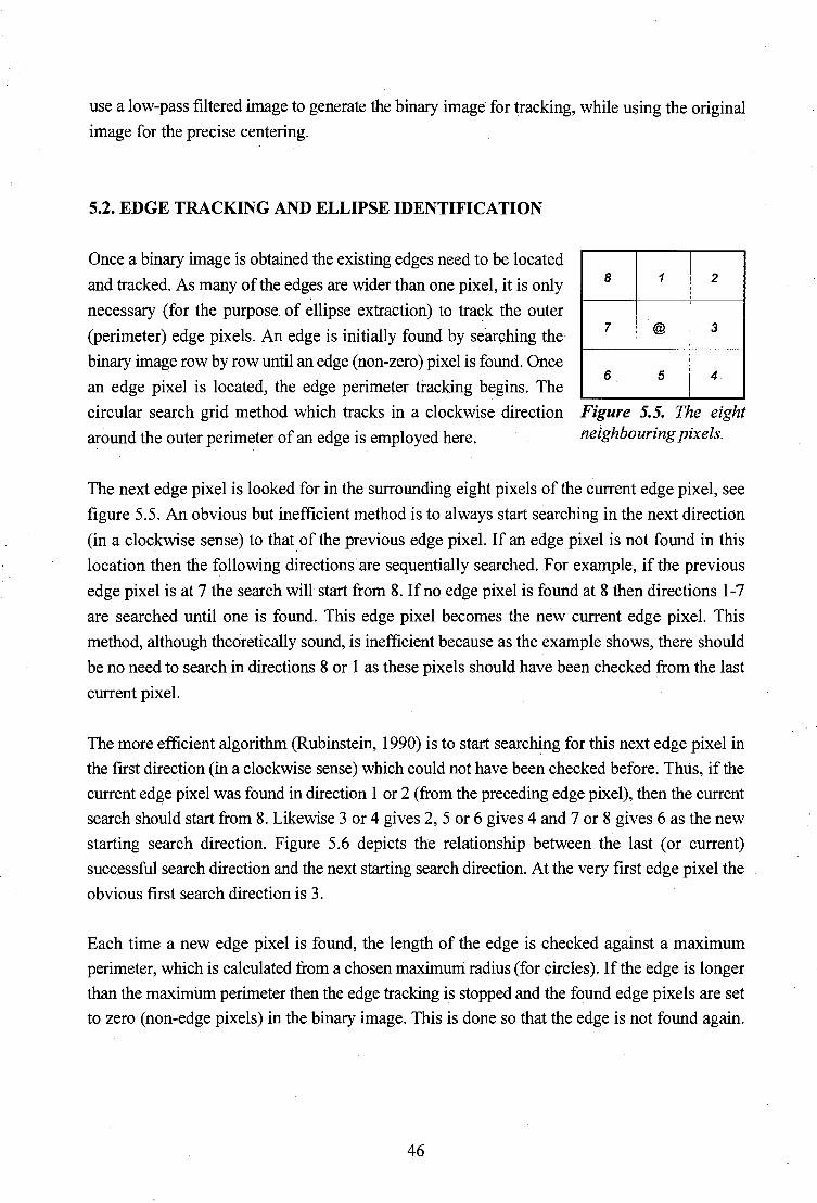
use a low-pass filtered image to generate the binary image for tracking, while using the original

image for the precise centering.

5.2. EDGE TRACKING AND ELLIPSE IDENTIFICATION

Once a binary image is obtained the existing edges need to be located

and tracked. As many of the edges are wider than one pixel, it is only

necessary (for the purpose of ellipse extraction) to track the outer

(perimeter) edge pixels. An edge is initially found by searching the

binary image row by row until an edge (non-zero) pixel is found. Once

an edge pixel is located, the edge perimeter tracking begins. The

8

7

6

1 2

@ 3

5 4

circular search grid method which tracks in a clockwise direction Figure 5.5. The eight

around the outer perimeter of an edge is employed here. neighbouring pixels.

The next edge pixel is looked for in the surrounding eight pixels of the current edge pixel, see

figure 5.5. An obvious but inefficient method is to always start searching in the next direction

(in a clockwise sense) to that. of the previous edge pixel. If an edge pixel is not found in this

location then the following directions are sequentially searched. For example, if the previous

edge pixel is at 7 the search will start from 8. If no edge pixel is found at 8 then directions 1-7

are searched until one is found. This edge pixel becomes the new current edge pixel. This

method, although theoretically sound, is inefficient because as the example shows, there should

be no need to search in directions 8 or 1 as these pixels should have been checked from the last

current pixel.

The more efficient algorithm (Rubinstein, 1990) is to start searching for this next edge pixel in

the first direction (in a clockwise sense) which could not have been checked before. Thus, if the

current edge pixel was found in direction 1 or 2 (from the preceding edge pixel), then the current

search should start from 8. Likewise 3 or 4 gives 2, 5 or 6 gives 4 and 7 or 8 gives 6 as the new

starting search direction. Figure 5.6 depicts the relationship between the last (or current)

successful search direction and the next starting search direction. At the very first edge pixel the

obvious first search direction is 3.

Each time a new edge pixel is found, the length of the edge is checked against a maximum

perimeter, which is calculated from a chosen maximum radius (for circles). If the edge is longer

than the maximum perimeter then the edge tracking is stopped and the found edge pixels are set

to zero (non-edge pixels) in the binary image. This is done so that the edge is not found again.

46

If the edge tracking comes back to the very ·'·

first edge pixel, then the process must decide

whether this edge belongs to a circular feature

or not. If the tracked edge closed before

reaching the maximum perimeter limit, then

the detected edge pixels are used as

observations in a best-fitting ellipse least

squares adjustment. The computed a0 is

applied as one.ofthe test criteria for accepting

or rejecting an edge as a circular feature. The

test criteria are:

(1) the computed a0 is less than a

certain value (this ensures the

edge is elliptical). This value

is usually set at 0.5 pixel to

allow for some noise and

sampling effects along the

(2)

edge,

the computed ellipse centre is

inside the bounding rectangle.

of the tracked edge (which

6

current direction

6

4

8

~

7

5

l

I 4

next starting

direction

/ 2

4

~

Figure 5.6. The circular search grid.

might not happen if an ellipse is fitted to a curved edge for example),

8

2

2

(3) the ratio of semi-major and semi-minor axes of the computed ellipse is within a

certain tolerance. A value of 0.3 has been used here but this could be changed

depending on the application.

(4) the computed radii are within the minimum and maximum radii selected. Values

of 1 pixel and 30 pixels have been used here as the minimum and maximum radii,

but again these can be changed for different image scales and/or made stricter for

specific applications.

If a feature passes all these tests it is accepted and the ellipse centre and its extent (window size)

are recorded for future processing. This ellipse centre.can be used as an approximation for the

centre of the circular feature in later processing stages. Occasionally small rectangular edges are

accepted by this ellipse test, thus an additional test constraint (which has not been tested here)

could be that the edge direction changes gradually. This would require the calculation of the edge

direction, which can be computed from the arctangent of g/gx or approximately from the

direction, 1-4 in figure 5 .1, of the maximum gradient.

47

The edge must be erased from the image so that it is not found again. Various ways of doing this

are possible:

(1) The tracked (perimeter) edge pixels are set to zero. If the edge is thicker than one

pixel, this method will peel the outer layer away and the inside layer will be

detected as another feature. Thus, one feature could be found a number of times

if the edge is fairly thick.

(2) Set all pixels within the bounding rectangle of the tracked edge to zero. This

method is easy to implement, does not have a problem with thick edges as in (a),

but it is possible for this routine to erase portions of other, as yet undetected

features if these features should lie within the bounding rectangle of the current

feature. This method· will also erase any smaller features which are contained

within the current feature.

(3) Find all the edge pixels which are connected to this tracked perimeter edge. All

these edge pixels are then set to zero. This method results in no information loss

of other edge features, however this is the most time consuming of the three

methods described here.

Version (3) should be used when edges are liable to be thick, features are very close together or

when some circles lie within other (closed) features. If edges have been pre-thinned down to one

pixel, then version (1) should be used (version (1) has the same effect as version (3) for edges

with single pixel width). Version (2) could be used if the edges are thick, the features not too

close to one another and circles within features do not exist or can be ignored, as version (2) is

faster than version (3). Version (3) has been implemented in this system.

Once the current feature has been analysed and erased from the edge image, the routine continues

by searching for the next edge pixel from the position of the first edge pixel of the erased feature.

The routine continues until the entire image has been processed.

As mentioned before, the output from this stage is a list of approximate target centre coordinates

and target window sizes which are used by one .of the precise centering techniques described in

chapter 6.

48

One of the most basic procedures in any digital photogrammetric system is determining the

precise location of control points in the digital images. In close range applications, circular

targets are generally favoured for use as control points, hence the precise location becomes a

centering problem. Altogether five techniques have been investigated and programmed as

options in the measurement system. Each of these technigues are formulated, discussed and ~~'·?&~zy~~. f~j}Jf::W:,~~::·.~~I

analysed in this chapter. ·., · , · ·· · ·

6.1 SLOPE INTERSECTIONS

The first target centering algorithm is a least squares intersection of all slope elements

(Forstner and Gulch, 1987). The slope element (slopel) at a pixel is defined as the straight line

passing through the centre of that pixel with an orientation (<I>) equal to the direction of the

maximum grey level gradient at that pixel. The line equation for a single slope element at

(yi,xi) is:

x .cos<I> - y .sin<I> - l = 0 I I I I i (6.1)

where 1 is the distance between the coordinate system origin and the line. Thus the intersection

of all slopels (y0,Xo) (which is an estimate for the centre of a circular feature) can be found by

solving the following linear system:

v(y,x) = x0cos<!>(y,x) - y 0sin<!>(y,x) - l(y,x) (6.2)

with weights equal to the absolute (maximum) gradient squared:

P(y,x) = IY7gl2 (6.3)

Using the conventional matrix notation of v = Ax - 1 and letting gxik and gyik denote the x and

y direction components of the grey level gradient at a pixel in the jth row and kth column of

the window surrounding the circular feature, gives:

49

-gxll gY11

JVg11 J JVg11 J -sin<l>11 cos<l>11 Vil

-gxl2 gY12 -sin<l>12 cos<l>12

JVg12 J JVg12 J v12

v = A = (6.4)

Vmn -sincpmn coscpmn -gxmn ~ gYmn

. JVgmnl j\lgmn I

l· 12

x = ( ::) , I = = (6.5}

1vg11 l2 0 0

0 JVg12J2 0

p = (6.6)

0 0 j\7gmn1 2

50

This results in the normal equation system:

(6.7)

The gradients gx and ~ at each pixel could be computed using equations' 5. 2 and 5 .4 from

chapter 5. The summation is taken over all the pixels in the target window. The solution is

computed in the normal way:

(6.8)

The slope elements of a general ellipse do not all intersect at the centre of the ellipse, but the

solution provides suitable results for near circular target images (see results in 6.5.4), because

of the symmetrical distribution of pixels with large grey value gradients (i.e. large weight).

6.2 WEIGHTED CENTRE OF GRAVITY

The weighted centre of gravity technique using the grey value as a weight is a common area

based centering routine (see for example Trinder (1989), Wong and Ho (1986), Gustafson and

Handley (1992) or Ruther and Parkyn (1990)). This technique and a similar one using the

square of the grey value as weight are covered in this section and have been programmed as

options in the measurement system.

6.2.1 ... with Grey Value as Weight

This routine (and the grey value squared one) is formulated for a white target on a black

background, however if the reverse situation exists then the grey values should be inverted for

the equations to hold. Equations 6.9 and 6.10 are derived using moments:

- ~yg Yo - -­

~g

51

(6.9)

(6.10)

in which g is the grey value.

6.2.2 ... with Grey Value Squared as Weight

The equations for the centre of gravity using the grey value squared as weight are

Yo - ~yg-2 ---

~g2 (6.11)

XO - ~xg2 ---

~g2 (6.12)

Using the grey value squared as weight, as opposed to grey value, reduces the influence of the

window.position on the. computed centre coordinates. However it is also more sensitive to

noisy pixel grey values.

For both methods, improvements in accuracy can be obtained by only including those pixels

with grey values greater than th~ background level as ?bservations. This removes the effects

of window position if the whole target is within this window (compare table 6.1 to table 6.3

later in this section).

6.3 BEST-FITTING ELLIPSE

This method most closely models the actual centering problem for circular targets. Best-fitting

ellipse routines although used fairly often (mentioned in, for example, Schneider and Sinnreich

(1990), Fritsch (1989) and Wiley and Wong (1990)), appear to be not as popular as the

weighted centre of gravity method, prob~bly because of the extra computing time and the more

complex approach. The method is broken into four steps here:

(1) sequentially tracking (finding) all the perimeter edge pixels,

(2) defining each slope line,

(3) computing suh-pixel edge locations along the slope line and

(4) solving a least squares best-fitting ellipse adjustment.

52

The first stage can be accomplished as described in section 5.2. These edge pixels are

approximate indicators of the edge· and can be used together with the provisional target centre

to define a straight line approximately perpendicular to the edge (slope line) along which the

edge operator can be applied. However, in the developed measurement system these slope lines

are calculated differently. As the output from the circle location stage provides an approximate

target centre and bounding target window coordinates, the slope lines are defined by the

window edge points and the centre. This avoids the need to track the edge a second time and

does not adversely. affect the edge location accuracy because the computed slope lines remain

approximately at right angles to the edge for reasonably well defined targets (see figure 6.1).

Sampling at sub-pixel . positions (by

interpolation) at steps of one pixel along this

slope line, from outside the target edge to

the target centre, results in a string of grey

values which are used as input to a sub-pixel

edge location algorithm based on the

moment preserving method (Tabatabai ·and

Mitchell (1984) and Mikhail et al (1984)).

The first three sample moments are:

1 . m. = -I:s 1

' n (6.13)

I""' \ ~~ ~-

""' ~ ~\ ~

"' r-...

ir "'- \ ~ , """

\ ;' ' ""' " I\ ' '"'-\

I'\

' ,

\. /

"' '/ ......_.

........ ...,,,,, , ~- ~ -

Figure 6.1. The ellipse window showing three computed slope lines.

for j = 1, 2, 3. The summation is taken over all the samples (s) from 1 ton (number of

samples). The moments.are then used to find the edge location:

(6.14)

c (6.15)

k = !:c1 - c > 2 J4 + c 2

(6.16)

53

Here k is the number (non-integer) of samples below the edge. Thus the edge location, x,

relative to the first sample (in sample units) is given by:

x = k -1

2 (6.17)

In these investigations five positions outside the edg~ are sampled unless another close edge

is encountered (by looking at the grey value changes).

Once the sub-pixel edge locations have all been found they are used as observations in a least

squares best-fitting ellipse adjustment. The general equation for a rotated ellipse is:

[ cos<!>(x; :-x0) - sin<l>(y; -y0)]2 [sin<l>(x; -x0) + cos<l>(y; -y0)]

2

~~~~~~~~~~- + ~~~~~~~~~~-(6.18)

where

yi,xi ..... coordinates of point on ellipse perimeter

y0,Xo ..... coordinates of ellipse centre

a, b ..... semi-major and minor axes of ellipse

<I> . . . . . rotation of ellipse

The combined adjustment model is used for these observation equations. Precision measures

for (y0,Xo) are obtained in the usual manner. The best-fitting ellipse centering method provides

high accuracy centering for well defined targets except when a target borders on another

unrelated edge which will adversely affect the ellipse edge location.

6.4 LEAST SQUARES TEMPLATE MATCHING

Least squares matching (Ackermann, 1984, Grue~, 1985, Rosenholm, 1987) with a template

can be used for centering circular targets, assuming that a suitable" template can be generated

to closely resemble the general structure of the many targets. High accuracy is obtainable,

however the precision will vary from point to point depending on the resemblance of a

particular point to the template being used for the matching. Radiometric parameters should

be included to minimise this problem. For high speed centering (matching) the grey level

gradients required in this model can be computed from the template patch, thus allowing the

54

formation and inversion of the normal equation matrix before the iterations start. The

formulation of the general least squares matching model is given in chapter 8.

6.5 TESTING WITH IDEAL TARGETS

6.5.1 Generating an Ideal Ellipse with Direct Fall-Off

An ideal target ellipse is one in which the area, within the ellipse has a grey value of 255

(saturation) and the area outside has a grey value equal to the background level. Due to the

discrete nature of pixel grey values (one value for an area of a pixel), the pixels through which

the ellipse border runs will have grey values between the background and saturation levels.

This grey value will depend on the amounts of the pixel area inside and outside the ellipse

boundary.

Each pixel within the ellipse window is processed to obtain a grey value. The ellipse window

can be made. square and its position and size computed from the ellipse centre and the semi­

major axis. A pixel acquires a grey value equal to the background level if completely outside

the ellipse, 255 if completely inside the ellipse or a value obtained using equations 6.20 to 6.22

if on the border.

A point at (yi,x) is considered inside an ellipse if

[cos<f>(x; -x0

) - sin¢(y; -y0)]

2 [sincj>(x -x0

) + cos¢(y; -y0)]

2

---------- + I ~ (6.19)

a2 b2

otherwise the point is outside the ellipse.

The method used to evaluate the grey values of the ellipse border pixels is as follows. The

border pixels are sub-divided into 256 sub-pixels (16x16 sub-pixels per pixel). Each corner

of each sub-pixel is evaluated to see whether it falls inside or outside the ellipse border. The

number (0-4) of enclosed (inside ellipse) corners, 11c, is computed for each sub-pixel. The sub­

pixel is given a grey value, gs, of

(6.20)

55

Each sub-pixel in the current pixel is processed in this way, after which the pixel's unscaled

grey value, g', is computed from the sum of the sub-pixel grey values:

(6.21)

The value of g' will range between 0 and 256, thus to obtain a value between the background

and saturation (255) grey levels we must scale g' using:

g 1(255 - b) g=b+-----

256 (6.22)

in which b is the background grey value and g is the correctly scaled grey value of the pixel.

All grey values are evaluated as floating point numbers up until the windows are written to an

8-bit image file.

6.5.2 Fall-Off Functions

The ellipse generated in section 6.5.1 is an ideal digitization of an ellipse. Fall-off functions

model target blurring caused by de-focusing, over-illumination and electronic effects. There

are a number of methods which could be employed to generate and apply these fall-off

functions. For the series of tests below, the target fall-offs were obtained by convoluting the

image containing the ellipses with a two-dimensional 7x7 discrete normal distribution with a of 1 pixel. Trinder (1989) performs a similar convolution for generating blurred targets.

6.5.3 Random Generation of Ideal Ellipse Parameters

A total of 196 ideal ellipses at regular grid intervals of 30 pixels, shifted by random amounts

of +0.5 to -0.5 pixels in x and y, were generated in a test image. The radius a of each ellipse

was randomly generated between three and eight pixels and the corresponding radius b was

set between +303 to -303 of the value of a. The ellipse rotation angle, <I>. was also randomly

generated between 0 and 360 degrees. A background of grey level 60 was set.

56

6.5.4 Centering Results

The ellipses were located in the test image as described in chapter 5. To test the effects of

choosing. a different scaling factor (for a of image gradients) two cases were processed: the

first with scale = 2 and the second with scale = 1. The scaling factor slightly influences the

size of the target windows computed in the location stage.

The first set of results with scale = 2 is presented in table 6 .1 and the results with scale = 1

are shown in table 6.2 below.

Centering Results (scale = 2), units: pixels

Method RMS ax RMS ay RMS t.X RMS t.y max t.X max t.y

0 - - 0:008 0.008 -0.033 0.027

1 - - 0.031 0.032 0.088 0.089

2. - - 0.087 0.091 0.216 0.211

3 0.003 0.003 0.004 0.004 0.015 0.017

4 0.02 0.02 0.002 0.002 0.007 0.009

Table 6.1. Centering results using ideal targets (gradient threshold scale = 2).

Centering Results (seal~ = 1), units: pixels

Method RMS ax RMS ay RMS t.X . RMS t.y max t.X max t.y

0 - - 0.007 0.005 -0.028 0.022

1 - - 0.031 0.031 0.109 0.081

2 - - 0.085 0.087 0.252 0.208

3 0.003 0.003 0.004 '0.004 0.022 0.019

4 0.02 0.02 0.002 0.002 0.009 0.009

Table 6.2. Centering results using ideal targets (gradient threshold scale = 1).

The methods are numbered as follows:

0: Slope intersections

1: Weighted centre of gravity (WCG) with grey squared as weight

57

2: WCG with grey as weight

3: Best-fitting ellipse

4: Least squares template matching

The RMS ax and ay columns are the root mean squares of the standard deviations of all the

centre coordinates as obtained from the last two methods. The RMS ti.X and ti.y columns are

the root mean squares of the differences between calculated and known coordinates of the

ellipse centres. The max ti.X and ti.y columns are the maximum differences for each method.

The template used for the matching was generated in the same way as described in section

6.5.1, with integer centre coordinates, a = b = 8 pixels and <I> = 0 degrees. A Gaussian fall­

off was also computed for this ellipse. A window of 25x25 pixels centred about the exact

ellipse centre was then used as the template. In the matching, all six affine parameters (see

section 8.2.1) were included in the solution which was iterated until the shift corrections fell

below 0.001 pixels and the other corrections dropped below 0.005. The results of the matching

are for 189 of the 196 ellipses, the remaining seven patches did not converge, because of the

large difference in scale between template and these ellipses.

The results show that the larger windows used resulting from a scale of 1 slightly improve the

centering results. The best-fitting ellipse method faithfully reflects the standard deviations of

the centre coordinates, while the least squares matching is out by a factor of 10, when

comparing to the RMS ti.x and ti.y of the two methods.

As can be clearly seen from the results, the two WCG methods are the least accurate. This can

be attributed to the windows not being exactly centred about the ellipse centre, thus

introducing a bias in the resulting coordinates. This argument is justified by the accuracy

differences between using grey value squared or grey value as weight. The grey value squared

method is less influenced by the window position than the grey value method, because the

relative weight differences between centre and background pixels are considerably larger in

the grey value squared case.

To overcome this window problem, thresholding has traditionally been used to good effect,

as in Trinder (1989) and Van der Vlugt and Ruther (1992). In these techniques, a threshold

value is subtracted from the original grey value. If the resulting grey value is negative it is set

to zero. Thus pixels with original grey levels below or equal to the threshold value do not

contribute to the solution as they have zero weight.

Various techniques can be used for determining a threshold value which separates background

from target. One simple and fairly fast way is to use an interactive approach where the user

changes the threshold value (the graphics palette can be thresholded) until a suitable binary

58

image is found by inspection. Thus one threshold value is chosen for the entire image. In order

to automate the thresholding it is more convenient to use the grey values within the target·

window to make a suitable choice. Wong and Ho (1986) use:

t = (6.23)

with t being the. threshold value, gs the smallestgrey value in the window and gm the mean

grey value in the window. This method will. depend on the size of the window relative to the

target because of the mean pixel value used in the computation. A value more independent of

window size would be:

(6.24)

with gb being the biggest grey value in the window.

Three further tests were carried out for the two WCG methods (1 and 2) using different

thresholding techniques:

a: t = 60 (actual background value)

b: using eqµation 6.24

c: using Wong and Wei-Hsin's formula (equation 6.23)

Centering Results (scale = 2), units:. pixels

Method RMS .c:.x RMS .c:.y max .c:.x max .c:.y

1t (a) 0.003 0:003 -0.008 0.009

2t 0.013 0.014 0.043 0.049

1t (b) 0.006 0.006 0~017 0.015

2t 0.003 0.004 .;0.012 -0.012

1t (c) 0.006 0.006 0.014 0.016

2t 0.003 0.004 -'0.010 0.010

. . Table 6.3. Centering results for methods 1 and 2 using ideal targets (gradient threshold

scale = 2) and three versions of window thresholding.

59

I

:!

The results are shown in table 6.3 for only the case of scale = 2, as the values in scale = 1

are almost identical because of the thresholding.

As can be seen there is a substantial increase in accuracy when any of the three threshold

subtraction techniques is used. The probable reason for the inferior values in case 2t(a) is that

most of the background pixels within the window have values slightly larger than 60 (due to

the convolution applied), thus they still influence the solution but not nearly as much as when

no threshold subtraction is used.

6.6 TESTING WITH REAL TARGETS

A flat wooden surface with a regular 10 by 10 grid of retroreflective targets was made for a

centering repeatability test of targets in real images. These targets which were 8mm in

diameter were spaced at approximately 3cm intervals. The wooden surface was painted with

a mat black paint (blackboard paint) of low reflectance. The test involved the capturing of ten

sequential images (over approximately 11 seconds) of the target field and then performing

centering on all the images for all 100 targets using all of the five techniques above. As

discussed and evaluated in section 4.1.1.5, PLL synchronisation errors cause random line jitter

in the order of 3/lOOth of a pixel (up to 0.13 pixel in the worst case) for the ITC camera used

in this test. The line jitter obviously affects.the repeatability of the centering in the x-direction

and as such is an important factor when analysing the results of this test.

The ITC camera, which had been continuously switched on for a full day,. together with the

PIP-512B MATROX frame-grabber were used for the image capture. The offset and gain were

adjusted so that the centre of the targets had grey values of about 245 and the background had

grey values of approximately 25.

The thresholding used in conjunction with centering algorithms 1 and 2 was equation 6.24.

The convergence criteria for the least squares template matching (method 4) was 0.001 pixel

for the two shifts and 0.005 for the remaining affine parameters. A 17 by 17 template for the

LSM method was generated using the same technique as described in sections 6.5.1and6.5.2

with.both radii equal to 5 and a zero rotation. They-shear parameter was held fixed for all the

targets in this test. Table 6.4 shows the results of the repeatability test.

The RMS V x and RMS '? columns are the root mean squares of the x and y coordinate

residuals of every point in each image for that particular centering method. The max Vx and

max VY columns are the maximum residuals occurring with each method. The RMS values are

computed using equation 3.2 in chapter 3 (with a similar equation for they-coordinate).

60

Repeatability, units: pixels

Method RMSVx RMS VY max vx max Vv

0 0.017 0.011 0.053 0.037

1 0.012 0.008 0.052 0.027

2 0.011 0.007 0.049 0.028

3 0.011 0.008 0.035 0.027

4 0.011 0.008 0.040 0.028

Table 6.4. Repeatability of target centering methods using 10 images acquired with PU

line-.rynchronisation.

The repeatability reaches 11I1 OOOth of a pixel in X and 7I1 OOOth of a pixel in Y, with slightly

poorer results for the first method (intersection of slope elements). The poorer RMS V x values

are due to the line jitter as described earlier. If ~ixel-synchronous sampling or digital

transmission were to be used instead of the PLL synchronisation then the RMS V x can be

expected to be of the. order of the RMS Vy values. An important point which emerges from the

results is that the centering repeatabilities are a factor of about 2.5 times better than the

random line-jitter repeatabilities, thus showing that the centering process can partially

compensate for the random line jitter error if the target covers a number of image lines.

Obviously the larger the target extent on the image, the less influence random line-jitter will

have on the target's coordinates. The average image extent of the target windows in this test

was 17 lines by 14 columns.

The next part of the test was to compare the target coordinates of the different centering

routines. This was done separately for each image so that the line-jitter differences between

the images were avoided (although line-jitter still had an effect within each image). For each

image, the RMS residuals (of x and y) were computed for each method comparison. There

were five methods to compare, thus ten method comparisons were performed for each image.

Thereafter the average RMS residuals (over the ten images) for each comparison were

computed. The individual RMS values are computed using equation 3.2 in chapter 3 except

that the subscript i refers to the method and not to the image. The average RMS Vx and RMS Vy values are depicted in table 6.5 and the corresponding overall maximum residuals in x and

y are shown in table 6. 6.

61

Comparisons (Ave. of RMS of residuals) units: pixels

Methods 1 2 3 4

Ox 0.028 0.025 0.022 0.016

y 0.012 0.013 0.016 0.021

1 x 0.006 0.012 0.014

y 0.008 0.013. 0.018

2x 0.009 0.012

y 0.008 0.011

3x 0.011

y 0.011

Table 6.5. Average of the ten RMS Vx and RMS Yyfor each image for the method

comparisons.

Comparisons (Max. of residuals)

units: pixels

Methods 1 2 3 4

Ox 0.110 0.097 0.087. 0.079

y 0.043 0.064 0.074 0.082

1 x 0.019 0.031 0.037

y 0.029 0.053 0.042

2x 0,028 0.028

y 0.024 0.029

3x 0.035

y 0.033

Table 6. 6. Maximum x and y residuals for the method comparisons.

From these results a few observations and conclusions can be made. The RMS of the residuals

are all less than 3/lOOth of a pixel with especially methods 2,3 and 4 agreeing very well with

each other (the RMS of the residuals is about l/lOOth of a pixel). The maximum residuals

when comparing methods 2 and 3 are especially good (0. 028 pixels in x and 0. 024 pixels in

62

y, equivalent to a maximum coordinate discrepancy of 0.056 pixels in x and 0.048 pixels in

y). The agreement between methods 2 and 4 is also very good and thus one sees that the

weighted centre of gravity (grey weight) agrees extremely well with the LSM technique and

the best-fitting ellipse method even though the WCG method requires far less time to execute.

The WCG method can thus be recommended for systems needing a fast but accurate centering

technique. The good relationship between methods 1 and 2 is to be expected because of there

high similarity. The results associated with method 1 are slightly worse than those for method

2 when these methods-are compared to 3 and 4. This is probably due to the grey value squared

weighting scheme of method 1 amplifying errors caused by noise in the images.

Other strong edge gradients very close to a target can deteriorate the centering, especially the

best-fitting ellipse routine, and thus should be avoided if possible when designing a control

field for calibration or exterior orientation. This phenomenon often occurs with the targets on

the rods and bars in the control fields described in section 4.3 due to regions of shadow close

to these targets.

The best-fitting ellipse routine offers a good method of obtaining reliable precision estimates

for the centering process. This was not the case for the LSM technique when testing on the

ideal targets of section 6.5.

63

7. CAMERA ORIENTATIONS

7.1. THE PROBLEM OF POINT IDENTIFICATION AND CAMERA ORIENTATION

To orientate a camera in space the image points used for the resection need to have known three

dimensional object coordinates. Assuming all these image points have their object coordinates in

a list, the task is to automatically identify the image points in the same naming/numbering scheme

as in this list. This is usually easily done by the human operator who has a good knowledge of

the way the points are numbered and their relative positions in a particular image scene. However

the task is far more difficult to automate on a computer especially when using plain circular

targets. However additional information or constraints can be used to simplify the identification

procedure. A similar problem is posed by the process of relative orientation. Here two lists of

image point positions need to have their relationships established. Additionally, once the relative

orientations have been computed the points need to be identified if an absolute orientation is to

be computed.

Once a set of points has been identified, the system must be able to determine adequate provisional

value.s from which further processing can successfully proceed. A number of semi-automatic and

automatic approaches to identifying points and computing orientations are described below.

7.2. SEMI-AUTOMATIC INTERACTIVE ORIENTATION

The manual identification of all control points on an image can be tedious when many exist. The

following reliable routine has been developed for the semi-automatic identification of control

points in an image. The routine is performed once the image coordinates of all the targets have

been accurately determined. The procedure can be divided into three sections:

(1) interactive identification of eight control points and computation of an initial

orientation,

(2) automatic identification of remaining control points and

(3) update orientation.

1. Eight control points (for redundancy) are manually identified on the displayed image using a

mouse cursor. An initial direct linear transformation (DLT) resection, see Abdel-Aziz and Karara

64

(1971), is then computed from these eight points and the eleven DLT parameters are stored.

Easily identifiable points can be used to make this stage more time efficient, however the points

must be well distributed in space for a reliable DLT resection. Practically it is generally easiest

to identify the same points in all images if they are visible. The computed a0 from the DLT

adjustment is used a:s a criteria for accepting or rejecting the user's input. The a0 is displayed for

the user to view. If the input was rejected the user has to re-identify the eight points. The

advantage of using the DLT formulation is that no approximate values are needed to obtain

convergence, however a minimum of six control points need to be identified to solve for the

eleven DLT parameters. The user is prompted to identify eight points in order to obtain a slight

redundancy, to increase the reliability of the orientation.

2. All the known control points in object space are projected into image space using the

approximate eleven DLT parameters computed in step one. Each observed image point is now

compared (by image distance) to every fictitious (projected) image point. The fictitious point with

the associated smallest distance is chosen as the correct match for that observed image point.

However, if none of the distances are smaller than a certain threshold then that point is considered

as a non-control point. This threshold can be computed by scaling the a0 computed from step one.

A fairly large scale of ten was consistently used to accommodate the unmodelled lens distortions

on points dose to the edge of the image. If two or more observed image points are matched with

one fictitious point then the observed image point with the smallest image distance to this point

is accepted as the true match and the others are marked as non-control points. The average image

distance for all matched points is computed and displayed for the user to view. This parameter

could also be used as a criterion for globally accepting or rejecting the results of this stage or for

testing individual matches.

3. A new DLT resection is computed using all the identified points. In case some control points

were not identified before, step 2 is repeated with the latest DLT parameters. A final DLT

orientation is then processed and the final eleven DLT parameters are used to compute initial

estimates for the interior and exterior orientation parameters to be used in a later bundle

adjustment which takes additional parameters into account.

Other techniques besides the D LT can be used for determining provisional. values from a minimal

amount of points. For example Hinsken (1988) proposed a non-singular method of determining

the photogrammetric resection, by using a different parameterization of the rotation matrix.

65

7.3. AUTOMATIC ORIENTATION

A number of methods have been used for automating the orientation process, almost all of these

using some unique characteristics of the points. For example, in Clarke et al. (1994), an open

planar rectangle (one side missing) is used to automatically identify four points (two intersections

and two endpoints) which are used to compute the camera orientations with a geometric vector

method.

A more direct approach is to uniquely mark each target, usually by means of a binary code. Van

den Heuvel and Kroon (1992) report on using binary coded targets to perform automatic

identification. The binary code ring surrounds the target and is comprised of a unique starting

code and the remaining identification number. The number can be read off by sampling at regular

angular intervals around the code ring.

Huang and Trinder (1993) use a process of different combinations to solve the correspondence

problem between image and object point lists. They compute approximate 3-D coordinates of

seven image points in a local system relative to the camera centre and axis by using the known

size of the targets in image and object space. These computed point positions are used to match

distances with the control file to obtain combination sets. Each viable combination set is tested

by a DLT resection until the correct combination is reached. This method cmild work well if the

coordinate approximations are good, but it is not a very reliable approach, as a partial occlusion

. for example would result in the process performing a huge amount of attempts before finding the

correct combination. Huang and Trinder show that there are 2.4 x 10e+9 possible combinations

when using 7 points out of a control list of 25 points. Working with much larger control lists then

becomes totally impractical with this method.

Completely automatic orientation is thus still a problem unless distinct targets or unique target

layouts are used. Coded targets seem to be the best solution for general purposes if the large target

size (needed for a reliable identification and centering) is acceptable.

7.4. AUTOMATIC ORIENTATION WITH DEDICATED SET-UPS

Camera orientations can be fully automated.when using a dedicated set-up (cameras basically kept

in the same position). A once off interactive resection procedure determines the starting position

and orientation of the cameras. Additional update orientations, and if required calibrations, can

be automated due to the abundance of good a priori knowledge. The known 3-D coordinates of

66

control points can be used with the latest station parameters (orientation elements) to determine

good approximations within the image coordinate system_ to start accurately determining the latest

image coordinates of the control points. Any of the search and centering routines can be used

depending on the implementation requirements. Thresholding, target detection and the centre of

gravity method offers high speed centering and orientation for on-line systems. Least squares

matching although slower can be adopted for some systems especially if a modified approach is

used. As mentioned in section 6.4, this involves using the template patch instead of the search

patch to determine the grey level gradients for the A matrix. This modification results in an

unchanged A 1l> A matrix and hence the normal equation matrix can be set up and inverted before

the iterations start. This normal equation matrix inverse (QxJ can also be used by all other target

matchings when using the same template.

Haggren and Haajanen (1990) use templates of natural features to perform repeated location in

image sequences. The templates are derived from real images in the actual orientation positions

of the cameras in an initial teaching/learning stage. This allows for a pre-calculation of the Qxx

matrix and for the shaping parameters (scales and shears) to be eliminated.

An extension to this idea could be the use of the previous search patches as the current template

patches. This would allow slowly varying factors such as lighting conditions and patch shaping

effects to be more easily accounted for with fewer iterations, however a new Qxx matrix would

need to be computed for the templates after each image sequence.

Heikkila (1990) describes the set-up calibration and automatic update orientation procedure of an

on-line photogrammetric system, in which the approach described in Haggren and Haajanen is

used for locating the control features and the orientation is automatically updated if the image

coordinates reflect a changing geometry after a few image sets. Proper statistical analysis is used

here for deciding whether an update orientation is needed or not.

Automatic update calibrations of a dedicated photogrammetric patient positioning system (Van der

Vlugt and Ruther, 1992) are performed by using the previous calibration parameters and the

known 3-D coordinates of the control points. In this system the user controls the frequency of the

calibrations and decides whether the automatic identification of the control points are correct

before allowing the system to re-calibrate.

67

8. IMAGE MATCHING

8.1 GEOMETRIC CORRELATION

Geometric correlation is the term given here to purely geometric methods of matching point

(feature) sets in different images. ln other words only the constraints imposed by the

collinearity equations are used for the matching. These methods require that all points

(features) have already been accurately located in all the images. Most of these techniques are

very similar in principle, the task being to find conjugate points which most closely satisfy the

collinearity condition. They employ either epi-polar planes, epi-polar lines, 3-D intersections

or combinations of these to define the (same) collinearity criteria. If image distortions are

taken into account, as is done by for example Dold and Maas (1994), the epi-polar line

changes into a slight curve. The effect of distortions should be properly dealt with for best

possible reliability.

In the following steps a geometric correlation method, developed in this work, is described.

The method uses 3-D intersections and back projection to define the collinearity criteria. For

the following description the term reference image refers to only one of the images and the

term search images refer to all the other images (one or more) which are b(!ing used in the

matching. The reference point is a single point from the reference image which is currently

being matched with the points from the search images. A test point refers to a point in one of

the search images which is currently being tested as a match. The basic steps are:

1. For every reference point in the reference image repeat steps 2 and 6.

2. For every test point in all the search images repeat steps 3 to 5.

3. Compute a 3-D coordinate by using the x and y image coordinates of

the current reference point and the x image coordinate of this test point.

4. Back project the 3-D coordinate into the search image containing the

test point correcting for any known image distortions.

5. Calculate a y image coordinate discrepancy (dy) between the back

projected y coordinate and the observed y coordinate of this test point.

The test point is marked as a 11 candidate match 11 if dy is less than a

predefined threshold, Yt· The values of dy and the 3-D coordinates

computed in step 3 are stored with this candidate match.

68

6. This final step involves selecting the "correct match set" from all the candidate

matches for the current reference point. The number of test points within the

correct match set can range from zero to the number of search images.

If within the candidate matches there exist two or more "common" (similar) 3-

D coordinates (stored in step 5), then these candidate matches are chosen as the

correct matching set. This occurs when there are three or more imaging rays

to a point (in object space). Two candidate matches from the same search image

cannot have "common" 3-D coordinates, unless they are virtually the same

image point.

If no "common" 3-D coordinates exist (when the point appears on only two

images) the candidate match with the smallest dy which has a 3-D coordinate

within a defined "bounding volume" is accepted as the (only) correct match.

"Common" 3-D coordinates refer to coordinates that are within a small enough range so as to

be obviously describing the same surface point. This allowed range could be defined in object

space or as is done here in image space, by back projection of the 3-D coordinates of the

candidate matches into the other search images. The advantage of defining the range in image

space is that the range can be defined by a search radius of Yt· Thus, if the back projected

image points are withi~ this search radius in all search images, then the 3-D coordinates of

these candidate matches can be considered cortlmon for this purpose.

The "bounding volume" can be defined by the coordinates of the control (in a simple case) or

by using some known or estimated knowledge about the surface. The definition of even a large

bounding volume (from control) helps in rejecting apparently good (small dy) but incorrect

matches when only two imaging rays exist.

The image threshold, Yt• is chosen by using a multiple of the a0 obtained from the exterior

orientation of the cameras. If the value for Yt is too low some correct matches could be missed,

or if too high some incorrect matches could be.accepted (which will normally only happen if

there are less than three imaging rays for a point).

Two extensions to the basic steps outlined above would improve the matching technique. It is

best to match all points with more than two imaging rays first (by only retaining the found

matches with three or more rays) and then to move on and match the points appearing in only

two images. In addition once the possibilities on the current reference image are exhausted a

different reference image is selected until all possible points have been matched.

69

Geometric correlation works extremely well if conjugate points for matching can be extracted

from all the images to a high precision. This is possible with well defined high contrast

features which have easily extractable forms such as circles. However, it is not always possible

with lower contrast or complex features. Therefore this technique is ideally suited to fast

matching of targeted points but a more general algorithm such as multiphoto geometrically

constrained matching is better suited for matching various types of features.

8.2 MPGC MATCHING

Multiphoto Geometrically Constrained (MPGC) matching, proposed by Gruen (1985) and

thoroughly investigated by Baltsavias (1991), is used as a base for the matching procedure

developed in this thesis. MPGC matching combines area based matching and a modified

collinearity intersection into a single simultaneous least squares solution which solves for

X,Y,Z object coordinates and all image coordinates of a specific point in space. The

intersection formulation is modified in the sense that the image coordinates (except on the

reference image) are no longer fixed but are solved for as part of the overall adjustment

procedure.

The interior and exterior orientations are pre-calculated before the MPGC matching takes

place. The search space of the MPGC algorithm is geometrically constrained and thus an

almost one dimensional search space occurs. The width of the search space is controlled by

the weights of the observations in the MPGC adjustment. With very high weights for the

collinearity observations the search space becomes fully one-dimensional, being forced onto

the epi-polar "lines". Thus, assuming precise orientation parameters, the matching process is

considerably strengthened by these collinearity observation equations or geometric constraints

as they are often called.

Other very important advantages of the geometric constraints arise when more than two images

are used. Using multiple images (defined here as three or more images) not only increases the

reliability of the matching but further decreases the search space by forcing the search patches

to move along the epi-polar lines at specific step ratios (see Baltsavias, 1991). In addition,

Baltsavias showed that multiple images increase the chance of successful matching in cases of

occlusions, multiple solutions, discontinuities, perspective differences, poorish provisional

values and radiometric distortions. Gross error (blunder) detection also becomes easier when

multiple images are used.

Due to the factors outlined above, the MPGC algorithm was chosen as the matching model for

the developed system. Around this model, other supporting algorithms were developed and

70

implemented into a working unit to provide the automated surface measurement capabilities

of the system. Of special importance to the matching procedure are the following three tasks:

(1) extraction ofa suitably .dense distribution of good quality reference patches for

matching;

(2) determination of provisional values for all search image coordinates and the

3-D object coordinates for each reference patch and

(3) run-time blunder detection of the matching results as well as a post­

measuremertt blunder detection process.

Two methods of extracting reference patches of interest are covered in section 8.2.2. To

determine provisional values for the MPGC matching another two algorithms are discussed

in section 8.2.3, namely surface extrapolation from a DEM image and multi-image correlation

(MIC). The first is used as the default method of the system and the MIC is used to solve the

difficult cases as well as for the first surface point. The blunder detection scheme employed

is also outlined in section 8.2'.6. The flowchart in figure 8.1 indicates how these supporting

algorithms are combined with the MPGC matching to form a reliable matching procedure.

1 ~ Locate next reference patch

·1 of interest. Is one found?

Yes ,

Is this the first surface point ~

or did the last MPGC match Yes No - fail?

•• , I Extrapolate height I I MIC I I No

Yes from DEM image I

.I MPGC I Has this point I matching 1· failed MPGC matching

after using MIC? ·~

Is the match successful and does it pass the gross error No

test?

Yes

.. I Update I IDEM image

Figure 8.1. Flowchart of the matching procedure.

71

- - .\

8.2.1 MPGC Matching Least Squares Formulation

Only a brief summary of the least squares model used by the MPGC matching is given here.

For a more detailed description and explanation of the formulation the reader is referred to

Gruen (1985) or Baltsavias (1991). The derivation is given assuming known camera

orientations and for a single surface point.

The reference patch taken from the reference image can be modelled by a function f(x,y) and

the matching search patch taken from the ith search image (with a total of n search images) can

be modelled by gJx,y). Due to noise, perspective distortions, radiometric differences and other

factors the two, functions will not be equal, thus

"" j{x,y) - e.(x,y) = g.(x,y)

I I (8.1)

where ei(x,y) is a true error function associated with search patch i. The position of gJx,y) in

the ith search image needs to be estimated. The final position can be described by x and y

shifts from an initial approximate position. To model the perspective differences and other

systematic image deformations additional shaping parameters are introduced. The parameters

of the affine transformation are used for this patch shaping. The transformation of the grid

points in the ith search patch is given by:

in which:

atti• blli

a12b b21i

a2ti• b12i 0 0 x j, y i

x. I

Y;

0 0 = an.

I + at2 .x;

I + a2t Y;

I (8.2)

= bll. I

+ b12 .x;o I

+ b21 Y;0

I

are the x and y shifts of search patch i;

are the x and y scales of search patch i;

are the x and y shears of search patch i;

(8.3)

are the pixel coordinates of the grid points in the initial position of

search patch i;

are the pixel coordinates of the transformed grid points.

The six affine parameters need to be estimated from equation 8.1 which must first be

linearised. The linearised form of equation 8.1 is:

72

0 ag;0{x,y) ag;

0(x,y)

j(x,y) - e1.(x,y) = g

1. (x,y) + dx + dy ax ay

(8.4)

Also, differentiation of equations 8.2 and 8.3 gives

(8.5)

(8.6)

and to simplify let

(8.7)

(8.8)

Substituting equations 8.5 to 8.8 into equation 8.4 yields

0 0 + g dbll + gy X; db12. + g Yi db21.

Y; i I I Y, I

(8.9)

Note that it is also possible to include radiometric parameters in this formulation, however

these are left out here as they are corrected for separately within the iterations.

Equation 8. 9 represents the observation equations for the matching of the search patch i to the

reference patch. These observation equations can be written in the classical form

v =Ax.-! 11 I I 11

(8.10)

73

in which

(8.11)

(8.12)

A,. = (g x, (8.13)

0 11 = j(x,y) - g; (x,y)

I (8.14)

Equation 8 .10 forms a subset of the grey level observation equations used in the MPGC

matching. There is one of these subsets for every search patch/image used in the matching (i.e there are n such subsets).

There are 2(n + 1) collinearity observation equations describing the perspective projection of

the matching point into the reference image· and into the search images. These take the usual form

x - x + dxd J.

P1 J (8.15)

(8.16)

in which dxdj• dydi are distortion correction terms and j denotes the image (0 ... n), image 0

being the reference image. The shifts of the image patches can be included in these collinearity equations by letting

x = x + dx. j OJ J (8.17)

Y = y + dy. j OJ J (8.18)

74

where (Xoj• y0j) are the initial estimates for the jth image coordinates of the surface point and

(dxj,dyj) are the patch shifts in the image coordinate system. The reference patch shifts are

obviously zero throughout the iterations. Usually the pixel to image transformation for CCD

cameras is defined by equations 4.1 and 4.2 in chapter 4. Differentiation of equations 4.1 and 4.2 gives

(8.19)

dy = -ps dy img y pix (8.20)

or to follow the notation of this section we get

dx. = ps da11 1 xi J (8.21)

(8.22)

Thus, substituting equations 8.21 and 8.22 into 8.17 and 8.18 results in

(8.23)

y. =Yo - ps db 11 1 J Y1 I (8.24)

and equations 8.15 and 8.16 then become

(8.25)

(8.26)

remembering that da11j and db11j remain zero throughout the iterations when j = 0 (reference

patch). Equations 8.25 and 8.26, once linearised take the form of

75

(8.27)

in which x is the total parameter set correction vector of the MPGC matching and includes the

n parameter subsets xi (i = 1, ... ,n) and the three unknown point coordinates X, Y and Z. Thus

x can be written as

(8.28)

Equations 8.10 and 8.27 form a combined system connected by the patch shift parameters da11j

and dbuj· The least squares corrections for the total parameter set .are given by

x = (A Tp A + B Tp B)-1(A Tp l + B Tp l) 1 2 11 22

(8.29)

P 1 and ~ are the weight matrices of the grey level observations and of the collinearity

observations respectively. The weighting scheme employed in this work is discussed further

in section 8.2.4.

8.2.2 Extracting Patches of Interest

The interest patch extraction stage generates the set of reference patches to drive the MPGC

matching routine. The chosen patches must be evenly distributed over the surface (ideally in

object space), at a high enough density to adequately describe the surface and must have

sufficient texture to provide reliable matches with the search images. Good candidates for

matching success are reference'patches with strong gradients, preferably in more than one

direction. This is the primary reason for projecting patterns onto featureless or feature scarce

surfaces. Through the pattern design it is possible to provide distinct illumination edges on the

object surface and thus strong multi-directional grey level gradients in the images. The task

remains to extract reference patches at these positions of interest in the image. Two approaches

have been investigated to extract patches of interest, the first uses a simple edge operator and

the second uses the Forstner Operator. Both methods are discussed below.

76

8.2.2.1 Edge operator

The edge operator is a simple extension to the

generation of a gradient (edge) image as described in

section 5 .1. This edge operator extracts patches

centred about a pixel with a strong gradient.

Figure 8.2. A well textured reference As in section 5 .1, a gradient threshold needs to be patch with edge pixel at centre. computed for finding strong edge pixels from the

gradient image. Equation 5.6 is again used for the

computation of the gradient threshold. The value of

the scaling constant c must be set fairly low (0.5 to

1. 5) to obtain a dense distribution of edge pixels

above the threshold value. The edge pixels (after

thresholding) are thinned-out using a given mask size

(usually 7x7 pixels). This mask size can be altered if

Figure 8.3. A sub-optimal reference a higher or lower density of edge pixels is required. patch with edge pixel at centre. The thin-out method used here is taken from Forstner

and Gulch (1987) as used with the Forstner Operator.

Thin-out is achieved by placing a "mask" over each edge pixel. If another edge pixel within

this mask has a greater edge strength (gradient) than the central edge pixel, then this central

edge pixel is marked as a non-edge pixel.

Assuming that a suitably dense pattern has been projected on the surface, taking an image area

centred about an edge pixel should ensure

strong grey level gradients in the reference

patch. The algorithm stores all these edge

pixels for use as reference patch centres .

This approach generally works well and has

been successfully implemented for the

measurement of the test surface described in

section 10.3 . A typical well textured

reference patch taken from the projection of

a grid onto a surface is shown in figure 8.2.

However, if patterns of lower density are

used, sub-optimal patches will result. These

would generally still be matchable but

problems could result with the convergence of Figure 8.4. Interest points detected by the the shaping parameters . An example of such simple edge operator.

77

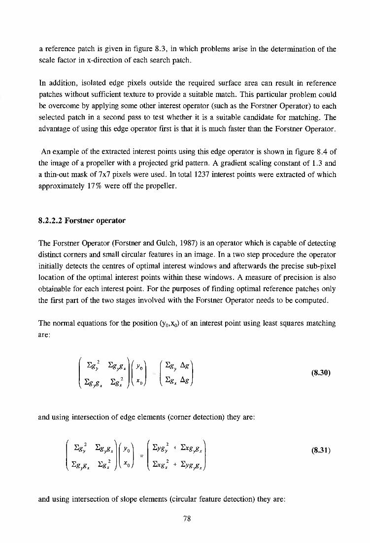
a reference patch is given in figure 8.3, in which problems arise in the determination of the

scale factor in x-direction of each search patch.

In addition, isolated edge pixels outside the required surface area can result in reference

patches without sufficient texture to provide a suitable match. This particular problem could

be overcome by applying some other interest operator (such as the Forstner Operator) to each

selected patch in a second pass to test whether it is a suitable candidate for matching. The

advantage of using this edge operator first is that it is much faster than the Forstner Operator.

An example of the extracted interest points using this edge operator is shown in figure 8.4 of

the image of a propeller with a projected grid pattern. A gradient scaling constant of 1. 3 and

a thin-out mask of 7x7 pixels were used. In total 1237 interest points were extracted of which

approximately 17 3 were off the propeller.

8.2.2.2 Forstner operator

The Forstner Operator (Forstner and Gulch, 1987) is an operator which is capable of detecting

distinct corners and small circular features in an image. In a two step procedure the operator

initially detects the centres of optimal interest windows and afterwards the precise sub-pixel

location of the optimal interest points within these windows. A measure of precision is also

obtainable for each interest point. For the purposes of finding optimal reference patches only

the first part of the two stages involved with the Forstner Operator needs to be computed.

The normal equations for the position (y0,Xo) of an interest point using least squares matching

are:

(8.30)

and using intersection of edge elements (corner detection) they are:

(8.31)

and using intersection of slope elements (circular feature detection) they are:

78

(8.32)

The sums in equation 8.30 to 8.32 are taken over all the pixels in the window.

The operator selects windows whose error ellipses are small and round. Looking at the three

normal equation matrices it can be noticed that the error ellipses will be identical for all three.

Thus the Forstner operator in addition to finding optimal windows for corner and circle

determination also finds optimal windows for least squares matching, therefore it is an

attractive method for locating good reference patches. It must be noticed that the centres of the

located windows do not generally coincide with the position of the optimal points which are

computed by solving either equation 8.31 or 8.32. Two parameters , wand q, are computed

to describe the size and roundness respectively of the error ellipse of a window:

1 detN w = = (8.33)

trN -1 trN

1 -(µ, - µ,) r 4detN (8.34) q (µ, + µ2) tr 2 N

in which µ1 and µ2 are the eigenvalues of the normal equation matrix. From equations 8.33 and

8.34 it can be seen that the normal equation matrix does not have to be inverted for the two

parameters to be computed. The parameter w increases for decreasing error ellipse size. These

two parameters are computed and stored for every window position in the image. A threshold

for w is needed to find windows of high interest. A threshold for q is used to retain windows

with a high roundness of their error ellipses. After thresholding the remaining windows are

thinned out to retain only local maxima of w. The thin-out procedure was described in section

8.2.2.1.

The final list of optimal window positions is used for the reference patch positions during the

MPGC matching. The interest operator, up until the thin-out stage, can be programmed as

described by Forstner and Gulch (1987) so that the time taken is independent of the window

size chosen. The thin-out is relatively fast as the number of pixels left to visit is small in

comparison to the total number of pixels in the image.

79

As a comparison with the simple edge operator already discussed, the same image in figure

8.4 is used as input for the Forstner operator to obtain the interest points shown in figure 8.5.

A mask size of 9x9 is used to generate the images w and q, the thresholds were set at 1.5 times

the average value of w and 0. 75 for q. A thin-out mask of 7x7 pixels (as for the edge operator)

is also used. A total of 1052 interest points were detected of which approximately 10 % were

off the propeller.

Figure 8.5. Interest points determined with the Forstner Operator.

8.2.3 Determining Provisional Values

In theory the Forstner operator is the

preferable method for extracting

patches/windows for matching because of its

design to pick out windows with small round

error ellipses for a matching task. On the

other hand surface features such as straight

lines will be better picked up by the edge

operator and so it is necessary to decide

which approach is more suitable for a given

image. As mentioned earlier, an approach to

consider is using a combination of interest

operators to extract interest points. Note that

it is possible to use the Forstner operator as

an edge operator by looking for windows

with elongated error ellipses.

MPGC matching, like most other non-linear least squares estimations, requires provisional

values for the unknown parameters . Area based matching requires fairly accurate

approximations for the patch positions in the search images. This pull-in range, as it is

normally called, is not fixed but depends on numerous factors including image content, patch

size and frequency of image patterns (such as projected grids). Generally speaking the more

accurate the approximations , the more likely a correct match results, thus the provisional

values should be determined as accurately as possible, without making the whole process

inefficient.

This task of determining all provisional parameter values needed for the MPGC matching can

be seen as the primary matching problem in that it is this task which actually determines the

correspondence between the reference patch and the search patches, as opposed to the MPGC

algorithm which provides the fine matching.

80

The provisional values needed by the MPGC matching for a single match are:

(1) X,Y,Z object coordinates of the surface point;

(2) x,y image coordinates of reference patch and all search patches and

(3) affine parameters for all search patches.

Y object I surface

images {fjJ

The affine parameters are usually set to one

for the two scales and zero for the shifts and

shears. The other parameters can all be

computed from the reference patch position

(obviously known) and only one other

coordinate (image or object), using the

known camera orientations and distortions.

Z (depth or

X ~ ~ /height) It is advantageous to use the depth ....._·=============:: ________ __. coordinate (usually defined by the z object Figure 8.6. The Z-coordinate axis defined as the coordinate axis) from which to calculate all object depth or height coordinate.

the others. The Z-coordinate is thus loosely

defined here as the depth coordinate or height, which is more or less perpendicular to the

general object surface as shown in figure 8.6. The provisional value problem thus reduces to

finding the correct Z-coordinate given the reference patch position, much like adjusting the

height of the floating dot onto the terrain surface in an aerial image stereo-pair.

A novel MIC search procedure, explained in section 8.2.3.1, which is geometrically

constrained has been developed for estimating the correct Z-coordinate. MIC is a reliable

method of determining provisional values when multiple images are used, so it has been

adopted as a back-up method for a less computation intensive (and less reliable) algorithm

using surface extrapolation. An initial surface match is obtained using MIC and all subsequent

surface point provisional Z-coordinates are then computed using the surface extrapolation

technique until an MPGC matching failure occurs (refer to figure 8.1). When a matching

failure occurs, the controlling routine assumes that an incorrect provisional value set was

passed to the MPGC sub-routine. The MIC search is then called and a new set of

approximations generated which are passed to the MPGC algorithm for a second matching

attempt.

8.2.3.1 Surface extrapolation for provisional height determination

Extrapolation can be very unreliable no matter what the task unless a priori information about

the parameter being estimated is known in some form or other. In the specific case of

extrapolating heights from an existing DEM, information concerning the modelled surface can

81

provide some checks and confidence in the extrapolat~d heights. For example if a surface is

smooth and continuous, extrapolation can be successful and reliable if the set of known heights

is dense enough. Many objects fulfill this requirement and those which do not can often be

divided into areas which do. This division is automatically handled by the support from MIC

and thus does not need to be modelled in any way.

Surface extrapolation for provisional height determination, which was also investigated by

Baltsavias (1991), works best with a smooth continuous object surface and a dense point

distribution. Good surface texture is a pre-requisite for ensuring a successfully matched dense

point distribution. Baltsavias decided against using this method as these requirements are often

not met in general. However the special case of projected patterns provides· the necessary

texture and the required density, thus the method can be successfully employed over the

smooth regions of an object's surface.

The height extrapolation. is incorporated into the matching procedure as follows. A "DEM

image" pixel-linked to the reference image is set up. Each pixel in the DEM image would

ideally contain the height of the object point imaged by the corresponding pixel in the

reference image. However as not every pixel in the reference image is matched and as the

DEM image is still growing at any one time, the pixels in the DEM image either contain a

height value indicating a successful match or a value defined as "no height" for a large number

of unmatched pixels. When a reference patch with strong texture is extracted from the

reference image, the z.:coordinate of the centre of this reference patch is calculated by

extrapolating the height at this pixel from the DEM image.

Extrapolation in the DEM image can be performed in a number of ways. One method is to use

both the surface gradients and surface heights of close successfully matched pixels, in

conjunction with a linear extrapolation to determine a "best-fit" estimated height for the

current pixel. A second much simpler method is to set the current pixel's associated height

equal to the closest successfully matched pixel.

Figure 8. 7. Extrapolation problems using simple (s) method of equal height and a more

complex (c) method employing gradient information from neighbouring points. The solid

circles depict previous successfully matched points and the hollow circles show the

extrapolated heights generated using the two methods.

82

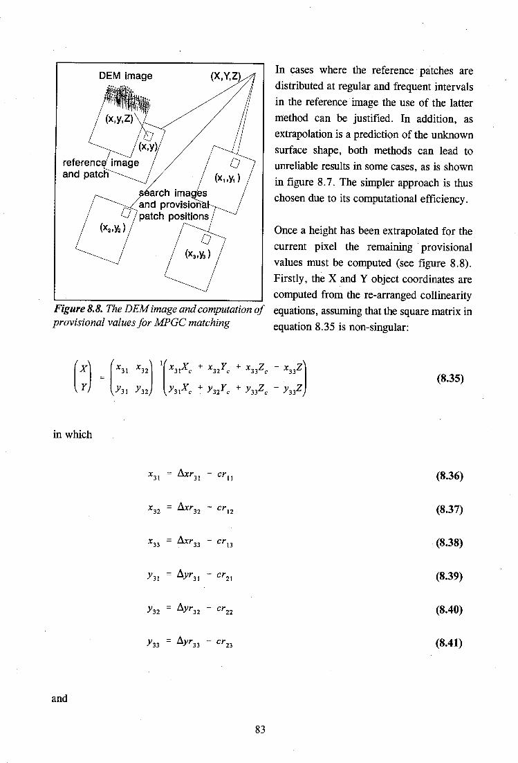
DEM image In cases where the reference patches are

distributed at regular and frequent intervals

in the reference image the use of the latter

method can be justified. In addition, as

extrapolation is a prediction of the unknown

surface shape, both methods can lead to

unreliable results in some cases, as is shown

in figure 8. 7. The simpler approach is thus

chosen due to its computational efficiency.

Once a height has been extrapolated for the

current pixel the remaining provisional

values must be computed (see figure 8.8).

Firstly, the X and Y object coordinates are

computed from the re-arranged collinearity Figure 8.8. The DEM image and computation of equations, assuming that the square matrix in provisional values for MPGC matching equation 8.35 is non-singular:

(8.35)

in which

X31 = Llxr31 - cr11 (8.36)

X32 = Llxr32 - cr12 (8.37)

X33 = Llxr33 - cr13 (8.38)

Y31 = Llyr31 - cr21 (8.39)

Yn = Llyr32 - cr22 (8.40)

Y33 = Llyr33 - cr23 (8.41)

and

83

(8.42)

~y = Y - Yp + dy a (8.43)

In a second stage the computed X, Y ,Z object coordinates are projected into all the search

image coordinate systems. This is achieved using the collinearity equations 8.15 and 8.16,

with initial values of zero for the distortion terms dxd and dy d· Once initial x,y image

coordinates are known the distortion terms can be computed and corrected values for x and y

are obtained. The image coordinates are then transformed into the original pixel coordinate

system using the known transformation parameters. It is very important to take account of

camera distortions in the determination of these provisional image coordinates because

distortions of over 60 microns are common towards the edge of a standard CCD image. The

provisional parameters are used by the MPGC routine and if successful (the matching results

pass a run-time blunder test) the resulting height is stored in the DEM image. If the MPGC

matching failed, the MIC routine is called to compute another estimate for the height of this

current surface point.

8.2.3.2 Multi-image correlation

Multi-image correlation (MIC) is an extension to the. traditional grey level correlation

technique. A correlation value, such as the normalized cross-correlation coefficient, describes

the similarity between two patches, and can be used for solving correspondence problems

between images. The basic steps of most correlation search procedures are:

(1) Extract a reference patch from the reference image. The conjugate position of

this reference patch in the search image must be determined.

(2) Define a search area and specific sampling positions (search patches) for

correlation, within the search image.

(3) Compute the correlation values (with respect to the reference patch) at each of

the defined sample positions.

(4) Find the sample position with the maximum correlation value. This position

indicates the search patch with highest similarity to the reference patch.

When no image orientation data is used, search correlation procedures correlate over an entire

2-D search area within the search image. When relative orientation between two images is

84

known, the search patch centres can be restricted along the epi-polar line in the search image.

This procedure is often used by photogrammetrists (see Wong and Ho, 1986; Claus, 1984 or

Dowman, 1984) to determine correspondences between two images.

The feature which makes the developed MIC

algorithm different and more reliable is the

simultaneous use of more than one search

image. The correlation search patch centres

are not only constrained along the epi-polar

"lines" of the search images but also to

geometrically consistent positions within

these lines. Figure 8.9 shows both these

constraints. A single correlation value

describing the similarity of these search

patches to the reference patch is computed at

each of the search steps (samples). Again,

the maximum correlation value of the

reference image and patch

reference ray with search steps 3

2,.,0 1d

GfH:J 1 2 3

search Images with search patches at geometrlcally consistent positions

along the epl-polar "lines•

Figure 8.9. The multi-image correlation (MIC) search concept. A search step (sample) number is shown next to the search patches and their associated object point.

samples indicates the search patch set with the highest similarity to the reference patch.

This extension is a natural progression from stereo-correlation and shares many of the

advantages of MPGC matching when more than two images are used. Sections 8.2.3.2.1 to

8.2.3.2.4 describe the MlC algorithm in detail, while section 8.2.3.2.5 reports on some tests

to show the characteristics and reliability of the method.

8.2.3.2.1 Constrained search space

As mentioned before, when using the information given by the camera orientations, the search

space is reduced into one dimension for two or more images. If image distortions are

accounted for, a ray in space is transformed into a curve on the image plane. Thus, epi-polar

lines (strictly speaking) should not be used if geometric consistency between the search patches

is required.

In order to create this geometric consistency between the search patches, it is appropriate to

drive the search procedure by generating search patch image coordinates from a varying height

coordinate along the "reference ray". The reference ray is defined here as the imaging ray

passing through the centre of the reference patch. An example, using figure 8.9, is given here

to the describe the search process. The search starts at height (Z-coordinate) 1 at point 1 along

the reference ray. The X and Y coordinates of point 1 can be computed from equation 8. 35. Both the search patch positions numbered 1 are calculated by back projecting point 1 into the

85

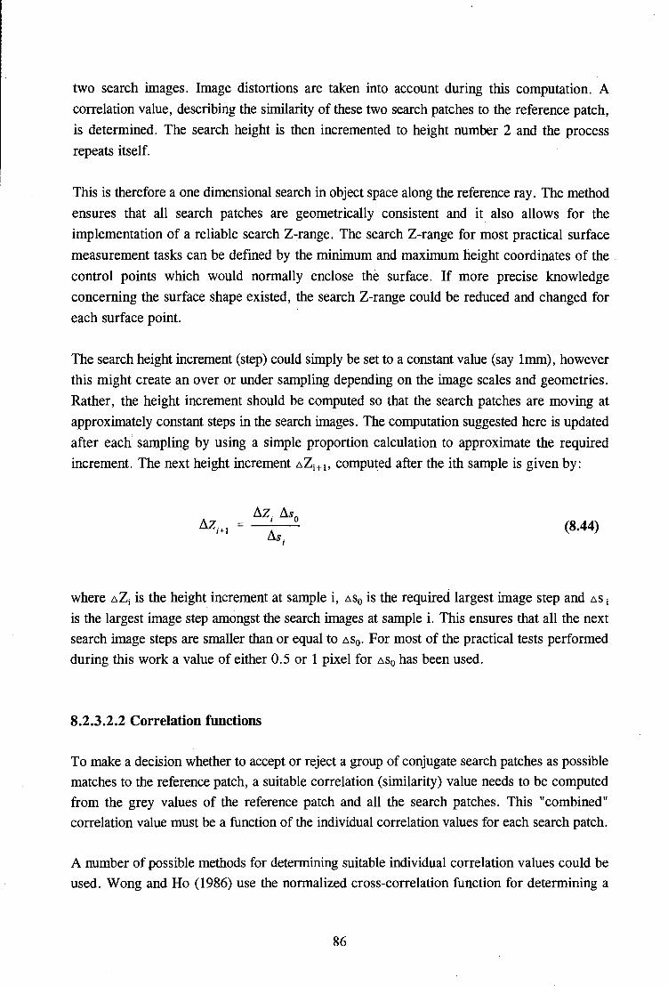
two search images. Image distortions are taken into account during this computation. A

correlation value, describing the similarity of these two search patches to the reference patch,

is determined. The search height is then incremented to height number 2 and the process

repeats itself.

This is therefore a one dimensional search iil object space along the reference ray. The method

ensures that all search patches are geometrically consistent and it also allows for the

implementation of a reliable search Z-range. The search Z-range for most practical surface

measurement tasks can be defined by the minimum and maximum height coordinates of the

control points which would normally enclose the surface. If more precise knowledge

concerning the surface shape existed, the search Z-range could be reduced and changed for

each surface point.

The search height increment (step) could simply be set to a constant value (say lmm), however

this might create an over or under sampling depending on the image scales and geometries.

Rather, the height increment should be computed so that the search patches are moving at

approximately constant steps in the search images. The computation suggested here is updated

after each sampling by using a simple proportion calculation to approximate the required

increment. The next height increment t.Zi+i. computed after the ith sample is given by:

(8.44)

where t.Zi is the height increment at sample i, t.s0 is the required largest image step and t.s i

is the largest image step amongst the search images at sample i. This ensures that all the next

search image steps are smaller than or equal to t.s0 • For most of the practical tests performed

during this work a value of either 0.5 or 1 pixel for Mo has been used.

8.2.3.2.2 Correlation functions

To make a decision whether to accept or reject a group of conjugate search patches as possible

matches to the reference patch, a suitable correlation (similarity) value needs to be computed

from the grey values of the reference patch and all the search patches. This "combined"

correlation value must be a function of the individual correlation values for each search patch.

A number of possible methods for determining suitable individual correlation values could be

used. Wong and Ho (1986) use the normalized cross-correlation function for determining a

86

correlation coefficient (value) between a reference and search patch, which is used in a ' ' '

matching procedure for two images. The normalized cross-correlation function is given by:

p

in which the summations are taken over all the pixels in the two patches and,

p the. correlation coefficient (value),

· a grey value from the reference patch,

a grey value from the search patch,

average of the grey values in the reference patch and

average of the grey values in the search patch.

(8.45)

The correlation coefficient, p, ranges from + 1 to -1; + l. indicates an exact similarity, 0

indicates no similarity and -1 shows that the search patch is a negative of the reference patch.

Equation 8.45 automatically allows for a radiometric equalisation of the mean and standard

deviation of the two patches. This correlation function needs to be maximised to find the most

similar search patch position.

A second method would be to compute the correlation value as the average of the absolute grey

value differences between -reference and search patch. The patches should be radiometrically

equalised to obtain a more reliable correlation value, .ti.g:

!::..g (8.46) m.n

where m and n are the dimensions of the two patches and gsc is a radiometrically corrected

grey value in the search'patch, given by:

a c ( -) g, g = g - g - +gr

s s s' a (8.47) g,

in which agr and ags are the standard deviations of the grey values of the reference and search

patches respectively. In this case the closer the correlation value is to 0 the more similarity

87

between the two patches. Thus, this correlation function needs to be minimised to find the

most similar search patch position. Vollmerhaus (1987) describes the use of this function,

which he calls the cross-difference-modulus-function, in some applications.

A combined correlation value must be computed from the individual correlation values of each

search patch. The average of the individual correlation values has been used in this work as

the combined correlation value. Only this combined (average) correlation value (not the

individual correlation values) is used for determining the correct match.

Both functions 8.45 and 8.46 have been investigated and both show similar results. The

normalised cross· correlation function has the advantage that the patches do not have to be

radiometrically equalised beforehand.

8.2.3.2.3 Location of correct maximum

For the discussion in this section the normalised cross correlation function is used as the

correlation function. However, the same argument would hold if the absolute grey level

difference function was used, except that the minimum correlation value (instead of the

maximum) would be searched for.

As will be seen later in the graphs (correlation profiles) in section 8.2.3.2.5, the correlation

values of patches which fall within areas of repetitive patterns show a fairly regular cyclical

pattern when plotted against the height. A number of local maxima occur .in these correlation

profiles and the problem is to determine the local maximum associated with the actual

matching search patch positions. Ideally the largest correlation value within the search space

identifies the correct match. This criteria for locating the correct match is easy to implement,

but can accept matches when none exist and can reject the correct match when its correlation

value is smaller than the largest value.

A number of factors can influence the correlation profiles to an extent where the correct match

becomes only a local maximum (as opposed to the absolute maximum). These factors can

include:

(1) the use of only two images,

(2) errors in the camera parameters,

(3) unmodelled search patch shaping,

(4) patch size,

(5) image resolution,

(6) search step size and

88

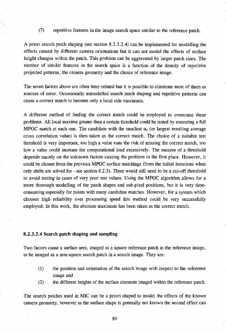
(7) repetitive features in the image search space similar to the reference patch.

A priori search patch shaping (see section 8.2.3.2.4) can be implemented for modelling the

effects caused by different camera orientations but it can not model the effects of surface

height changes within the patch. This problem can be aggravated by larger patch sizes. The

number of similar features in the search space is a function of the density of repetitive

projected patterns, the camera geometry and the choice of reference image.

The seven factors above are often inter-related but it is possible to eliminate most of them as

sources of error. Occasionally unmodelled search patch shaping and repetitive patterns can

cause a correct match to become only a local side maximum.

A different method of finding the correct match could be employed to overcome these

problems. All local maxima greater than a certain threshold could be tested by executing a full

MPGC match at each one. The candidate with the smallest a0 (or largest resulting average

cross correlation value) is then taken as the correct match. The choice of a suitable test

threshold is very important, too high a value runs the risk of missing the correct match, too

low a value could increase the computational load excessively. The success of a threshold

depends mainly on the unknown factors causjng the problem in the first place. However, it

could be chosen from the previous MPGC surface matchings (from the initial iterations when

only shifts are solved for - see section 8.2.5). There would still need to be a cut-off threshold

to avoid testing in cases of very poor test values. Using the MPGC algorithm allows for a

more thorough modelling of the patch shapes and sub-pixel positions, but it is very time­

consuming especially for points with many candidate matches. However, for a system which

chooses high reliability over processing speed this method could be very successfully

employed. In this work, the absolute maximum has been taken as the correct match.

8.2.3.2.4 Search patch shaping and sampling

Two factors cause a surface area, imaged as a.square reference patch in the reference image,

to be imaged as a non-square search patch in a search image. They are:

(1) the position and orientation of the search image with respect to the reference

image and

(2) the different heights of the surface elements imaged within the reference patch.

The search patches used in MIC can be a priori shaped to model the effects of the known

camera geometry, however as the surface shape is generally not known the second effect can

89

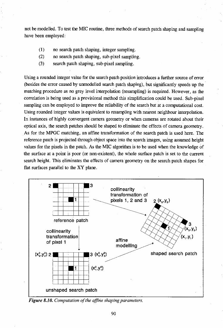
not be modelled. To test the MIC routine, three methods of search patch shaping and sampling

have been employed:

(1) no search patch shaping, integer sampling.

(2) no search patch shaping, sub-pixel sampling.

(3) search patch shaping, sub-pixel sampling.

Using a rounded integer value for the search patch posit1on introduces a further source of error

(besides the error caused by unmodelled search patch shaping), but significantly speeds up the

matching procedure as no grey level interpolation (resampling) is required. However, as the

correlation is being used as a provisional method this simplification could be used. Sub-pixel

sampling can be employed to improve the reliability of the search but at a computational cost.

Using rounded integer values is equivalent to resampling with nearest neighbour interpolation.

In instances of highly convergent camera geometry or when cameras are rotated about their

optical axis, the search patches should be shaped to eliminate the effects of camera geometry.

As for the MPGC matching, an affine transformation of the search patch is used here. The

reference patch is projected through object space into the search images, using assumed height

values for the pixels in the patch. As the MIC algorithm is to be used when the knowledge of

the surface at a point is poor (or non-existent), the whole surface patch is set to the current

search height. This eliminates the effects of camera geometry on the search patch shapes for

flat surfaces parallel to the XY plane.

2

1

reference patch

co Iii n earity transformation of pixel 1

,3

1 (x~ ,y~)

unshaped search patch

collinearity transformation of pixels 1, 2 and 3 2 (x2,y2)

affine modelling

shaped search patch

Figure 8.10. Computation of the affine shaping parameters.

90

Referring to figure 8.10, the image shaping of an individual search patch is achieved by

transforming three of the reference patch pixels (1,2 and 3) into this search image using

common height coordinates for each pixel. These resulting shaped positions of the three points

in the search image are given by (x1,y1), (x2,y2) and (x3,y3). The associated unshaped positions

of the points are (x01,y

01), (x0

2,y02) and (x0

3,y03), where:

(8.48)

(8.49)

(8.50)

r = (psize - 1)/2; (8.51)

in which "psize" is the size of the reference patch. The reference patch is assumed square and .

odd in size for these formula. The affine shaping parameters (as in equations 8.2 and 8.3) are

then computed from the following matrix equation:

0 0 -1 1 X1 Y1 0 0 0

all xt

0 0 0 1 0 0

a12 X1 Y1 Y1

1 0 0

0 0 0 a21 X2 Y2 x2 (8.52)

bll 0 0 0 1 0 0

Y2 X2 Y2

b12 1 0 0

0 0 0 X3 X3 Y3

b21 0 0 0 1

0 0 Y3 X3 Y3

The unshaped search patch pixels are then transformed using these affine parameters and the

search patch is resampled over this transformed grid at the sub-pixel positions. Bi-linear

interpolation is used in this work to compute the grey value at a sub-pixel position.

Deviations of the surface patch from a constant Z-value plane will result in unmodelled patch

shape distortions. If any of the pixels in the reference patch have reliable known heights, for

example from previous matches, then these can be used to improve the affine shaping by

91

assuming a slanted surface patch at this point. This could be used very well for applications

which use very dense sampling, but it has not been attempted during this work as the sampling

has not been dense enough in the surface measurement tests. As a by-product of the MIC

search the computed shaping parameters of the correct match could be used as provisional

values in the MPGC matching.

8.2.3.2.5 Increasing the reliability of the MIC process

The MIC algorithm can be said to be reliable when the correlation value of the correct match

is significantly larger than the other local maxima in the search space. There are a number of

ways of improving the reliability of the MIC search procedure. To show the factors

influencing the reliability a test set-up was designed. A regularly spaced white on black grid

was printed onto a sheet of paper which was fastened onto the back plate of the small control

frame later used for some of the surface measurements. Eight images, all about 60cm away

from the frame, were captured in the positions depicted by the small rectangles in figure 8 .11.

The entire grid and frame was. visible from each image.

0

0

0 0

0 0

0

0

0

0

0

8 H-t-H-H

~ 5

L....l...J.....o J....J.-L..L.1-oJ....J_J_LL_L.L__Lo--'-'-'

0 0 0 0

1 3 o rv

0 0

0 0

7

0 4

0

0

Figure 8.11. Plan view of control frame and image positions for the MIC test.

92

The camera was warmed up for a few hours

before the images were captured. Images 1

to 4 are arranged in a fairly typical camera

configuration. Image 5 is included to show

the effects of a close image to the reference

image (image 1 in this case). Image 6 is

incorporated to demonstrate how patch

shaping works, as well as to show how using

multiple cameras can compensate for

unshaped patches. Image 7 is used to

indicate the effects of camera base direction

(between reference and search image)

relative to the grid (or other pattern)

direction. Finally, image 8 is included to

show the effects of reference image position.

Different combinations of images and

shaping and sampling methods are used in

these tests. A constant reference patch in

image 1 is used for all the tests (except the

last) so that the results can be compared.

Each set of graphs depicts the results of a

complete MIC search (test) for the conjugate

search patches of the reference patch. The

graphs show a plot of the correlation values

at all the "search heights" (samples). The

final graph of each set is a plot of the

combined (average) correlation values,

calculated from the individual correlation

values of the search images plotted in the

preceding graphs. The search image number

is shown in brackets along the vertical axis.

'·' '·'

- 0.2

~ 0

a.-0.2

_,

iii "

...-~

• !J It: \\.. \

c • • ~

--~ •

i. " 'ii ..

uo 960 980 100010201040106010801100112011'0

z

'·' 0.6

- 0.2

:'.!. 0

'- -<l.2 .... -<l.8

_,

l c

ft. :p ~ '"" rm ~ .. -

" l ~

~

~ A n

li1 "'II> P& ~

~ 'Ill '!,

940 950 980 100010201D•0106010BD1100112011'0

z

........ 0.2

;:!, 0

Q.-o.2<---------1

-•+----------~~__, 940 960 980 100010201040106010801\00112011'0

z

-o.a;---------1 _,.,____,_ ______ __, 940 960 980 10001020104010601080110011201\40

z

The term "MIC profile" or just "profile" is Figure 8.12. MIC profiles of a test search using used in this section to describe the data of a the typical image positions 1, 2, 3 and 4.

graph. The arrows indicate the maximum

correlation value in each profile.

93

In all the graphs· which follow, unless

otherwise stated, image 1 is used as the

reference image, the resampling is computed

with patch shaping at sub-pixel positions, the

search step size, Li.S0, is set at 0.5 pixel, the

reference patch size is 9x9, the reference

patch is centred at a constant image position

and the MPGC computed height is

1077.34mm.

Figure 8.12 shows the four MIC profiles of

the first MIC search test .. The first three are

the individual profiles for the search images

2, 3 and 4 and the last one is the resultant

average profile. As can be seen from figure

8 .12 the individual profiles have large side

maxima, in. fact in image 2 there are three

maxima (including the correct one) with the

same value of 0. 98 and in image 4 a side

maximum is larger than the correct

maximum by 0. 01. However, even though

the individual profiles may indicate the

incorrect match (or height), the average

profile shows a clear maximum at the correct

height, larger by 0.23 than the next highest

maximum.

-"'8'j-----,-----------j

-~'!:'"'., -:o:,.,c-:,::::-'° ""'1000::-:-:I0,;::-20 =10•0::-:-:10"-•ot=osocc-:11c:-o01=120:-:-:<1 uo ' z

o.sr-----JJT----j 0,6 ,_---,,.,_.--------.0.--:-:-:<

'" t----///'---11.-------ilY----------- 0.2t---I'/---""'------' ~ at---------_,

0.-0.2+--~-------j

--0,Bt---------<

-·~--~--~____, 940 960 9801000102010•01oso1oao110011201uo

z

o.sr------a<Nhl!r---i 0,6t---,;r;m

;n 0.4j---=-tfl'll'f' .. ; o.2t-;;.-n;-~'-'!!'-------j

§ ot--Hril!J-------1 !. -o.zt---------i a.-0.4'j----------j

--0.Gt---------j

_,,,__,_ __ ~--~-940 gso gee 1000102010•01oso1oao110011201140

z

Figure 8.13. MIC profiles of a test search using two typical stereo images (1 and 4) and a close image (5) to the reference image (1).

This example clearly portrays that a successful method of improving the reliability is to

increase the number of images employed in the MIC search. It also shows the improvement

of MIC over usual stereo-correlation methods especially when encountering repetitive features.

The more images there are, the more unlikely it becomes that a significant local maximum

occurs in all images at the same search step, apart from the correct match point. In essence,

increasing the number of images increases the geometric constraint and hence the reliability.

Adding images also decreases the negative effects ·of unshaped search patches caused by

significant surface deviations from the normal.

As mentioned earlier in section 8.2.3.2.3 the MIC profiles have a cyclical pattern with a

certain frequency for each search image (in the case of repetitive surface patterns). The

individual local maxima which occur at the same height cause the biggest local maximum in

the resulting average profile. Thus an excellent way of significantly improving the dominance

94

of the correct match point is to use an image which ensures a very low frequency profile to

ensure that significant individual local maxima occur only at one search height. This is easily

achieved by employing an image very close to the reference image, such as image 5.

Figure 8.13 shows the individual profiles of search images 4 and 5 and their average profile.

The average profile again shows a clear maximum (0.16 larger than the next highest

maximum) at the correct height. Thus a close image to the reference image can significantly

improve the reliability of the MIC search although this image would not generally improve the

precision of the final MPGC match significantly. In the case of regular surface patterns the

closer a search image is to the reference image the lower the frequency of that MIC profile

becomes.

The profile associated. with search image 4 clearly shows the limitations of performing a

correlation with only one search image at a time, when repetitive surface features exist.

To show the effects of patch shaping the three search images 2, 6 and 4 are employed. Image

6 was in approximately the same position as image 3 except that it had been rotated about its

optical axis by about 45 degrees. The results of this MIC search are shown in the pgures 8.14a

and 8.14b. Figure 8.14a shows the profiles when patch shaping is computed during the MIC

search and figure 8.14b shows exactly the same search except with no shaping of the search

patches. The results without patch shaping show that the profile of search image 6 is very poor

even though in this case the maximum (p = 0 .19) occurred at approximately the right search

height. The patch shaping increases the local maximums significantly (largest p = 0.95) for

image 6. The profiles from images 2 and 4 remain fairly much the same because of the flat

grid and the fairly normal camera orientations of these two images. The average profiles show

a clear improvement for the patch shaping in this example. The patch shaping version has a

difference of 0. 3 7 between the maximum and the next highest local mCI:ximum and the

unshaped version has a difference of only 0.07. Thus the unshaped version, although much

poorer than the shaped version, has still correctly identified the matching point. This example

shows that the use of multiple images significantly improves the reliability when errors caused

by unmodelled shaping parameters e,xist. Surfaces of about 50 degrees from a constant Z plane

have been successfully matched by the MIC method in the shoe project described in chapter

10, even though the correct individual shaping parameters could not be applied in the search.

95

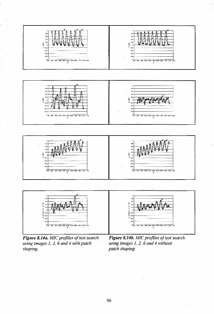
--H ~

~' ~

~ ,.; ill, ~ 11. ~ " "' -~ o+-~~lll--'~~~111'--'~!.li-'!ll;'--'!Ji---l!mr--"ia----I

a.-0.21--------------i

--O.•f--------------i --0.6j--------------i

-•+-----------------< 9.40 980 100010201DA01060\080110[}11201140

O.B 0.6

m,

z

HJ rli\ %

~ 0

"­ --0.2

ll'lll 1111!. '"" x

i,

% !!!I/Ii

(Ji p:i: ,< --O.• --0.6 ~ ·~ 'Ill

-I 940 960 980 100010201040106010801100112011.(0

z

0.2 .:!. 0

a.-0.2+---------------<

--0.B.f--------------i

-•+----------------< 940 980 100010201040106010801100112011'0

z

':;;' 0.4

ul 0.2 ,;

" E -o.2 ::-o.4f--------------i --0.6+---------------<

-•+-----------------< 940 960 980 10001020104010601080110011201140

z

Figure 8.14a. MIC profiles oftest search using images 1, 2, 6 and 4 with patch shaping.

O.B ' 0.6

o.•

~ 0

a.--0.2

--0.• --0.6

--0.B

-•+-----------------< 940 960 980 1000 1020 10•0 1060 1080 1100 1120 llAO

z

980 100010201040\0601080110011201140

z

O.B+------

0.6+----~

o.•

.:!. 0

a.-0.2+--------------l

--0.6+--------------l --O.B+---------------4 _,,__ ___________ __,

940 960 980 100010201040106010801100112011'0

z

0.6 j--------...----ml\-----i

'<t o,, +-~-Nlll--..--.c-Jtt..-Hc-fli'hA---i

.; 0.2 +-imlrttffllf'.!ilWi!IY\11-li;/j!-.i/Jrll~---i ,;

" ~:::f--------------i --0.6+--------------l

-o.B+--------------l

-•+-----------------< 940 960 980 1000102010401060108011001120\140

z

Figure 8.14b. MIC profiles oftest search using images 1, 2, 6 and 4 without patch shaping.

96

Another way of improving the reliability of

the MIC search, although slightly more

difficult to implement, is to position the

search images in such a way that the 11 epi­

polar lines 11 are slightly angled across the

grid in image space. This results in fewer

similar search patch positions as can be seen

from the circles in figure 8.16. To show

this, image 7 (fairly close to image 4) is used

with images 2 and 6 to improve the

reliability as compared. to the profiles of

figure 8.14a. The resulting profiles are

depicted in figure 8 .15. The profile

difference increases from 0. 3 7 to. 0. 50 due to

the 11 movement 11 of the third search image

from position 4 to position 7.

Epl-polar searcn , mage /

search lines, • • denote positions of high correlallon ~. ·

ii\• referimce·lmaQe 1 . search lmaae 4

Figure 8.16. Effect of the relative directions of the "epi-polar lines" and grid

The type of shaping and sampling also

affects the reliability of an MIC profile. As

mentioned before there are three basic types

discussed in this thesis: nearest integer

sampling, sub-pixel sampling and· sub-pixel

sampling with patch shaping. The effects of

these types of sampling can be seen in figure

) ifil ~·

o.• • ........ 0.2

!:', 0

"-

1\1 'Iii ~ ~ Ii.. '!)., - ~ . .. \. ... ---0.2

-0.4

--0.6

-o.s _,

940 960 geo 10001020104010&01oso110011201uo

z

I

0.8

0.6

0.2 ff!. ' '/\)\ ~·

~ 0

,..,, p~ ;

"­ --0.2 t~ ! !/!i//; .. '.I'. u

' ~ 1 .. -I

940 !160 980 10001020104010601080110011201140

z

- 0.2.,----,,-.......----..,--,-~-____,

c. 0

"- --0.2

--O.•

-1.+:-., -,,,,.:-co o=ao-::10'-oo =1020::-:'.10:<::"407.:'.1os::-:01=oao--,.,110~01=120:-:-:'1140 z

-1"".,-:c,.~o o=ao-:-:10"'"00 =1020:-:c10=.,"""1os::-:01=oao-:-c11r:-oo =1120:-:-:'1140 z

Figure 8 .. J 5. MIC profiles of the test search using images 1, 2, 6 and 7.

8 .17. Again, search images 2, 3 and 4 are used with reference image 1. Figure 8. l 7b shows

the MIC profiles using nearest integer sampling and no patch shaping, while figure 8. l 7a

shows the profiles using sub-pixel sampling with no patch shaping. These two sets of profiles

can be compared to figure 8.12 which shows the profiles using sub-pixel sampling and patch

97

shaping. The difference between the correct maximum and t:lle next largest maximum decreases

from 0.23 for patch shaping to 0.21 for unshaped sub-pixel sampling to 0.13 for unshaped

nearest integer sampling.

0.2 t--11\T+r'lrl'-ffi-+'m-P-+.q>...,.._o-1;,---I ~ 0 +--~rJ~"li~li.i'-"'•l,__.OJ,,.___,'f.~1~...,__~L__. a.--0.2+-------------1

--0.8+-------------1 -1+-------------<

9•0 960 980 100010201040106010601100112011'0

z

1 '" O.< . ['ll $. ft. d n

!# 1 :II., !'.!. 0 Q. --0.2

'Hi ~ ·'lll\,

'iii ~ " ; 1 !I ~ Iii • --0 ..

-1 940 950 980 10001020104010601080110011201140

o.e+----­o.o O.<

z

.:!. 0

a.-0.2+-------------1

--0.e+-------------1

-1+----------...,--, 940 960 980 10001020104010601080110011201140

z

-t 0.4 t--'!\rll!o--.ll;-;i;,lc--1'!1\-'1'ilf-J+-ill-1"----I ..,· 0.2+-H~~l.if-~-+4''-\'-JHl'l\\--I

"' a E -o.2 ......... -0.4+-------------1 Q. --0.6+-------------1

-1+-----------,-----; 940 960 980 10001020104010601080110011201140

z

Figure 8.17a. MIC profiles of the test search using images 1 to 4 with sub-pixel sampling (no patch shaping).

0.8 +--,,_.,_..,•,_.._,.,-il-• __,, .. _ .. _ ___, 0 .. t---111'-+r-+t--+t--++-r+-1~ -+-r1f--lfl..,______, 0-' +--++l--H,.-,>!;,-'.IR,.-H-+'+-1'+-i---l

I " ••l ~ or-~-~~w~~w~-~--1~19--'W-~J....--~ a.-0.2+-------------l

--O.e+-------------1

-1+-------------1 940 960 980 1000 1020 1040 1060 1080 1100 1120 11'0

z

0-' t--'!--'J'f--H--.l\-->-t<,......,;e----1

0.2 l-'H+~--±t-~-,H-+-r-iiilll'----1 !'.!. ot-H<>..mtt't++..l.+-l-+f-.l!''-ll!i---l a. -0.2 +---t-Hl.r-"'t-htt-'--"H'~ .... +---i

--0-' ,_.,.,_,..,_.....,_,..__.,... __ _,...__...__. -0.6·+-------~-----1

-1+-----------' 9.tO 960 980 100010201040106010!10110011201140

z

a.a +------i'f-~..._,lf-'!l---l

0.6 +----l'rll---ff-=-l-++++-+-1'LH'>--i , .. i---F',._-.!it-...,.,...,_,......,..._,.. ......... ---1

0.2+--....r-l±-m~f---------l

.:!. o+-;n++--,.__,r-------~

a.-0.2+-.~----------l

-1+-__ ,__ _____ ___, 940 960 980 10001020104010601080110011201140

z

0.6 T-,.--,!1'-=-'i'-..c-'l'l'-l;tr--+----1 ';" 0.4 t--11.-+llr-.ii.---.ltl,-jf!"l'=--</'+.J;-ffi-ilfb---I

!<')" 0.2 f--''j,-!',H,-lf;--ffi-l;-f-'"'!.S--H''-hHli~

"' g --0.:+---«------------1 E ~--0.•+-------------1

--0.6+-------------1

-1<-~--------,----< 940 960 980 10001020104010601080110011201140

z

·Figure 8.17b. ·MIC profiles of the test ·search using images 1 to 4 with integer sampling/no patch shaping).

98

If the surface slope at a point is unknown (as it usually is) and the camera orientations are

fairly normal, then patch shaping holds little if any advantage over the unshaped sub-pixel

sampling method. This is because either one could be superior as both would have errors in

their patch shapes due to unmodelled surface heights. Using nearest integer sampling is the

most time efficient method of the three, but as can be seen from the graphs it is not as reliable.

With higher resolution images at the same image scale and with fairly normal image geometry,

integer sampling could become the more viable alternative.

Another factor influencing the profiles is the choice of which image to use as a reference

image and its position relative to the search images. Using image 8 as the reference image with

search images 1 to 4 gives the average MIC profile shown in figure 8.18b. Using image 1 as

the reference image with search images 2, 3, 4 and 8 gives the average MIC profile shown in

figure 8.18a. Note that the reference patch position in image 8 is at the final MPGC matched

position when reference image 1 is used, but it is unshaped. The central position of image 8

(in relation to the other images) has two effects. The first is thatthe frequency of the profiles

is decreased (hence fewer significant local maximums) and the se.cond is that the number of

search steps decreases in this example from 181 for reference image 1 to 114 for reference

image 8. Both effects are caused by the fact that the search images 1 to 4 are all closer to the

reference image 8 than when image 1 was used as the reference image.

-- ---~ ; ~ ~ 0.8

0,6 •· • • 0,2 a ' ~ "' 111 '& 11 N

D ~

~ . . • .. ~

--0.2

-1.,___~~~~~~-< 94-0 960 980 1000102011l.t010601080110011201U.O

z

D.4 1 ~

- l'ii Ill. D.2

ilia ' fl ~ D

~ 'l' ~ '"'' ""1\1 --0.2 rm ~ ., • 'ff! i Ill ~ Ii ~ •

-1+--.-~~~~~~~ 940 960 980 1000102010401060\080110011201140

z

99

....---D.8 I :ti, J!l J

p D.6

~ D.4

~ 0.2 N

D ~ '

a.-0.2 i! • J,

--O.• %' " ! ~ . 'II \J l;J ... li

- ~

-1~-~~-~~-< 940 960 980 1000 1020 1040 1060 1080 1100 1120

z

....---~ ~ n 9

~ r~ I D.6

l . D.2

% I !'.?, D

% I a.~.2 .. J

--O.• ii,' i '!, ~ l ~ J Ill "U '\') l,J \J --0.6 - ~

-1

'" 960 980 1000 1020 1040 1060 1080 1100 1120

z

0.6

....... 0.2

.:!. 0

a.-0.2+-----------<

-1+---r---~------< 9•0 960 980 1000102010.t0106DIDB0110011201140

z

_ o.2t-~--i;-+---+------4 e o+-~----:i:----.oc'-'l'-~----4 a. --0.2 -l--V111--*--'irll-'llr-+-i--A--I

-1+-------~---< 9-40 960 980 1000102010.t01060108011001l201140

z

-;;; 0.6

.,;0.4+---"!f_,,______,..,.~

ti) o.2+---'!~lo1--t~

N D +---1111-V-lHl---"'---lll g--0.2+----------4 !,-o ... t----------4 a.-o.st----------4 -0.B+-----------<

-1+-----------< 940 960 980 1000 1020 1040 1060 1080 1100 1120 1140

z

Figure 8.1 Ba. M!Cprofiles using images 1, 2, 3, 4 and 8 (ref image 1).

~ 02 j--'i._,,_--,j"-'!r---T--+----1

.:!. ot--;i---.,---F--ll;---.tr---'\'-----1 a. -0.2 t----'l'------'l'--+------+--'l'---.1;---<I!

-O.•t--------1!.l!'----'llc--,lr---4-*-l

-O.Bt------~---1

_,,____.,..,.:--:-'":"---~~----< 940 960 980 1000 1020 1040 1060 1080 1100 1120

z

.::. , ot--±---c,----'1>--r--+--+----4 Q. --0.2-\---i.-4-~-+--A--.!J'--~<'-'f

-0.~ -1---'U---V-____,..,!'--'lo.j~-+-.l'-I

_, . .._ ____ ~ _ ___, 940 !160 980 1000 1020 1040 1060 1080 1100 1120

z

D.B+-------f------1

0.6 +---~Pm-------±-'f------1

-o.s+-----------<

-1"-----~----< 9•0 960 980 1000 1020 10•0 1060 1080 1100 1120

z

Figure B.18b. MIC profiles using images 8, 1, 2, 3 and 4 (ref image 8).

The effects of patch shaping, the sampling method, the relative positions of the images and the

number of images have all been shown in this section. the tests discussed here clearly show

the advantages of using the MIC approach over a standard stereo-correlation algorithm.

The resulting maximum average correlation value· from the MIC search procedure indicates

the height at which all the other provisional values for the MPGC matching can be computed.

8.2.4 Weighting of Observations

The weighting of observations for the MPGC matching plays an.important role in constraining

the solution and in obtaining meaningful standard deviations for the unknown parameters of

the adjustment.

100

·._! ----

The weight matrices P1 and P2 in equation 8.29 become diagonal matrices when using the

common assumption that the observations are uncorrelated. The main diagonal elements of P 1

can be computed using

(8.53)

in which o0 is the a priori standard deviation of unit weight and o1k is the a priori standard

deviation of the kth grey level difference observation. As absolute and relative standard

deviations of the grey level difference observations are difficult to obtain they are usually all

given the value 1, as is o0, thus P1 becomes an identity matrix in this case. The main diagonal

elements of P 2 are computed using

(8.54)

in which o2ic is the a priori standard deviation of the kth collinearity observation. Again these

standard deviations are usually considered as equal (in units of pixels). Their value is

dependent on whether full geometric constraints or partial constraints are being imposed on

the solution. In the former case, Baltsavias (1991) has shown that a standard deviation of 0.001

pixels is an appropriate value to use as it is practically data independent. If full constraints are

not wanted, as would be the case when the orientation parameters of the images are not ideal

but the correct match points in the images must be found, then a lower standard deviation

equivalent to the results obtained from the bundle adjustment can be used. However an

appropriate standard deviation for the grey level· observations then needs to be found, to

properly model the relative weights between the two types of observations.

The choice of a priori standard deviations for both types of observations has a large effect on

the resulting standard deviations of the 3-D coordinates. Fully constraining the solution by

giving a very small value to o2 usually results in too optimistic estimates for Ox, Oy and Oz if

one considers the uncertainties in the camera and station parameters which are not being

modelled. It is thus more appropriate to set o2 to a more realistic value equal to the o0 of the

bundle adjustment which was used for orientating the images. This only makes sense if the a

priori standard deviation of the grey level differences, o1, is given a realistic estimate so that

the relative weights between the two types of observations are correctly modelled. This can

101

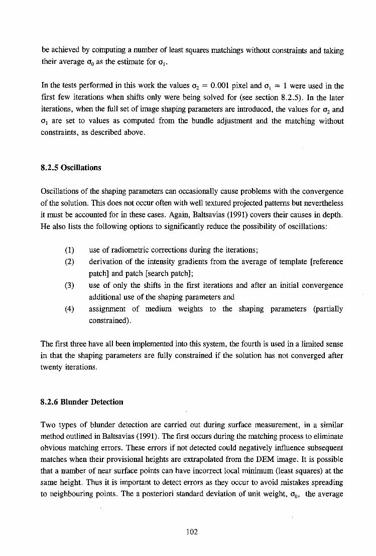
be achieved by computing a number of least squares matchings without constraints and taking

their average 0 0 as the estimate for 0 1•

In the tests performed in this work the values o2 = 0.001 pixel and o1 = 1 were used in the

first few iterations when shifts only were being solved for (see section 8.2.5). In the later

iterations, when the full set of image shaping parameters are introduced, the values for o2 and

0 1 are set to values as computed from the bundle adjustment and the matching without

constraints, as described above.

8.2.5 Oscillations

Oscillations of the shaping parameters can occasionally cause problems with the convergence

of the solution. This does not occur often with well textured projected patterns but nevertheless

it must be accounted for in these cases. Again, Baltsavias (1991) covers their causes in depth.

He also lists the following options to significantly reduce the possibility of oscillations:

(1) use of radiometric corrections during the iterations;

(2) derivation of the intensity gradients from the average of template [reference

patch] and patch [search patch];

(3) use of only the shifts in the first iterations and after an initial convergence

additional use of the shaping parameters and

(4) assignment of medium weights to the shaping parameters (partially

constrained).

The first three have all been implemented into this system, the fourth is used in a limited sense

in that the shaping parameters are fully constrained if the solution has not converged after

twenty iterations.

8.2.6 Blunder Detection

Two types of blunder detection are carried out during surface measurement, in a similar

method outlined in Baltsavias (1991). The first occurs during the matching process to eliminate

obvious matching errors. These errors if not detected could negatively influence subsequent

matches when their provisional heights are extrapolated from the DEM image. It is possible

that a number of near surface points can have incorrect local minimum (least squares) at the

same height. Thus it is important to detect errors as they occur to avoid mistakes spreading

to neighbouring points. The a posteriori standard deviation of unit weight, o0, the average

102

correlation coefficient of the final search patches and the number of iterations are compared

to absolute thr~sholds .after each match to detect gross errors.

Secondly, the results of all the surface point matches are assessed together to detect any

remaining errors. Other parameters besides the three already mentioned which can be used to

detect blunders are the height of a point and the values of its sh~ping parameters (scales and

shears) with respect to its neighbours as well as the values of its radiometric.parameters with

respect to all the surface points. Thresholds can be computed for each of the parameters by

evaluating

(8.55)

in which~ is the threshold of parameter p, p and aP are the average and standard deviation of

parameter p taken over the region (local or total) and c is a constant usually taken between 2 -

3. Many different approaches can be used as a rejection scheme. The one used here considers

a match a blunder if more than one of its parameters fail at the 3a level or if one of its

parameters. fail at the 4a level on a global basis. It must be noted that the values being tested

are not necessarily normally distributed (for a correct application of this test), however

equation 8.55 still provides reasonable threshold values to work with.

103

9. SURFACE ANALYSIS

9.1 LOCATING SURFACE PERIMETERS

In order for display routines, modelling packages or any other form of surface analysis pro~esses to correctly represent the surface, the surface edges/perimeters/borders must be coordinated and

marked as boundaries. For example, the surface display package SURFER, used for generating

perspective views of the test surfaces, requires a so called "XY blanking file" to prevent

interpolation of grid points outside the surface boundaries. In the case of the propeller

measurement described in section 10.1, a blanking file is used to prevent interpolation outside

the propeller blades. The SURFER package allows the blanking of areas (inside or outside) by

defining a list ofX and Y object coordinates. Thus to correctly display the propeller surface the

X and Y coordinates of a series of edge points around the propeller blades need to be computed.

In addition, to blank the centre piece, a series of edge coordinates from the central core need to

be added to the blanking list. Similarly, ifbreaklines are to be correctly modelled by a package,

they must be extracted from the images and coordinated in object space. This is particularly

important if the measured surface is being.'imported into a CAD/CAM package for detailed

measurements or ifthe surface is being used for CNC milling.

Therefore, the task is to extract these physical edges in the images without extracting the edges

caused by the projected pattern. An edge enhancement filter, based on the first derivative of the

Gaussian function, is used for this process. Canny (1986) investigated a computational approach

to determining an optimal filter for step edge detection. The first derivative of the Gaussian

operator closely approximates this filter and was used by Canny for his experiments. Other

researchers such as Sarkar and Boyer (1991) have also shown that the first derivative of the

Gaussian operator is a good edge detection filter, although not necessarily the optimal one. Van

der Merwe and Ruther (1994) use this filter in their combined feature and area based matching

process. The Gaussian or normal distribution curve is given by the function

-x2

G(x) 1 202

---e ffi. a

(9.1)

and the first derivative of the Gaussian is given by

104

-x2

G 1(x) = x 202 ---e (9.2)

A one dimensional filter formed from the Gaussian first derivative is computed by sampling the

function at steps of one pixel, with the centre of the filter coinciding with x = 0 in the function.

The width of the filter depends on the value of o chosen. Huertas and Medioni ( 1986) define their

Laplacian of Gaussian (LoG) filter to have a width of 8.5o, the same reasoning holds for the first

derivative of the Gaussian filter. To enhance edges occurring in areas oflow edge frequency (in

the space domain) a large o value (e.g. o = 3 or 4) should be chosen. Likewise to enhance edges

in areas of high edge frequency a small o value must be used (e.g. o = 1).

Because the projected patterns on the surface have a high edge frequency, a first derivative of the

Gaussian filter with large o is convolved with the imcige. In the case of the propeller surface, this

convolution enhances the physical surface edges because there are no significant radiometric

edges outside these surface edges. In addition the high frequency edges of the projected pattern

are significantly less enhanced. The results of this edge enhancement after thresholding can be

seen in the binary images of figure 9 .1.

The filter is convolved first in the x-direction with the original grey image to obtain _values of gx

(intensity gradient in x-direction) at each pixel. Similarly the same filter is convolved in the y­

direction to obtain values of gr Each of these gradient component images are separately

thresholded and only their local maxima are retained. The threshold is set relatively low at the

average value for gx and gY, but this still cuts out most of the unwanted weak edges. To find the

local maxima of the enhanced edge image in the x-direction a pixel is retained as a local

maximum if its edge strength (gj is greater than the edge strength of the pixel on its right or on

its left. A similar local maxima determination occurs in the vertical gY edge image.

With ideal step edges one can obtain equal edge strength pixels side by side. Therefore, an

expression such as "if the current pixel is greater (in terms of edge strength) than that of the pixel

on the right and if it is greater than or equal to that of the pixel on the left then mark this pixel

as a local maximum" should be used to retain only the one pixel as a local .maximum~ If this

"one-sided" test is not used adjacent pixels of equal edge strength would all disappear, even if

they were local maxima.

After determining the local maxima and applying the initial thresholding, the two gradient

component images are combined into a single gradient vector image, by computing the vector

of gx and ~ at each pixel. It must be noted that the vectors at pixels with only one' non-zero

gradient component are not all correct vectors as the one component may have been suppressed

105

'.·

by the local maximum determination and by the thresholding employed in this approach.

However this method seemed to produce less noisy branches along the strong major edges than

when computing the gradient vectors from the original components, as can be seen from the

binary edge images in figure 9 .1.

0 0 0 0 0 D 0 0 0 a

0 a 0 a 0 0 a 0 0 0

0 0

0 Q

0 0 a a ·.

0 0 ~~- oO 0 0 ~:~ oO . .

I 1 · 0 I 00 a 00 0 0

~ 0 0 0 0 0

0 0 0 a 0 0 0

!- 0 0 /"\! n ..... n ....

Figure 9.1. The binary edge (gradient) images shown here were both obtained with a a of 4

and the same threshold value. The final gradient vectors were computed from the thresholded

and maximised component images for the left image, while the original component images

were used for calculation of the final gradient vectors of the right image.

As can be seen from figure 9 .1 the left image has substantially less noisy branches. This is

especially noticeable along some of the retroreflective target edges.

A second automatic thresholding is performed by using a threshold value computed with

equation 5.6 from the gradient vector image. A good default value for the scaling constant, c, is

1, but this does depend on the image content. The average and standard deviation are computed

from the vectors at every pixel in the image. If the automatic thresholding is not satisfactory then

interactive thresholding of the displayed image can very quickly determine the best threshold

value for the gradient image. The threshold value is then used to generate a binary edge image

which is used for further edge tracking. Histogram analysis or local thresholding within smaller

image regions are two other possibilities for automatically determining a gradient threshold,

however every thresholding method is dependent on the image content and it is not possible to

106

identify a method which works in all cases. It is useful to have a fast interactive thresholding

routine for general purpose measurement. In dedicated set~ups, measuring the same type of object

with the same lighting, the problem disappears and a reliable threshold can easily be computed.

Once the binary edge image is generated, the edges need to be tracked and extracted. Before

tracking begins a thinning algorithm based on 8-connectedness (see Rosenfeld and Davis, 1976).

is used to ease the tracking procedure. Although the determination of local maxima in each of

the directions thins the edges, there are typically some edges in the combined gradient image

which still need thinning to one pixel width. A boundary tracking algorithm using the circular

search grid method, described in chapter 5, tracks around the outside of edges. An initial edge

pixel is searched for from the top and left of the image. Once a first edge pixel is located the edge

is tracked until the tracking returns to the same pixel, as seen in the left-hand box pf figure 9.2.

1st track 2nd track

Figure 9.2. Edge tracking using the circular search grid method The tracking is split into two stages. The digits represent the number of times each pixel.is visited during the tracking.

The number of times each edge pixel is visited during the tracking is recorded. The return to the

starting edge pixel is not counted here as a visit. As can be seen from the left hand side of figure

9.2 remaining edge pixels to the left and below of the starting pixel still need to be found. To find

the rest of the edge the same tracking procedure can restart at any of the edge pixels with one.

visit only (except at the original starting pixel again). This ensures that the whole edge is found

before returning to this new starting pixel (see the right-hand box of figure 9.2). Only once the

107

. "

whole edge, along all its branches, is tracked inthis way, is the edge stored in memory and wiped

from the binary image. Erasing the edge from the binary image is the most efficient way of

ensuring that it can't be found again.

The number of times an edge pixel is visited during the tracking is counted and this number can

actually be used to help categorise the type of feature and identify edge junctions. An edge pixel

with one visit means that this pixel is either an end point or part of a closed loop. End pixels can

be separated from closed loop pixels by counting the number of edge pixel neighbours, because

an end pixel only has one neighbour. Edge pixels with two visits are part of an ordinary branch

or junctions in a closed loop. Edge pixels with three visits are junctions along ordinary branches.

Four visits is not possible if the edges have been thinned to a point where the removal of any

edge pixel destroys the eight-connectedness of that edge.

Tracking the edge in this way is not the fastest way of doing it but it does allow for this useful

categorisation. Once all the edges have been tracked and extracted, end pixels (marked by the

tracking) can be joined to edge pixels of other segments if closer than a specified distance. The

system allows the user to select individual edge segments to write to file at specified steps along

the edge. This file can then be used as input into the MPGC matching routine to generate an XYZ

boundary file. Interactive edge editing is possible if required. The user can delete or add edge

pixels or delete whole segments. This is useful for problem areas where an important surface

edge becomes very weak within the image .

9.2 MATCHING OF SURFACES

Once a surface is measured it normally needs to be compared to a nominal model or a previous

measurement model to compute differences or deformations between the two. This is a fairly

simple task if the surface was measured in the same orientation and position within the 3-D

coordinate system, but it becomes much more difficult if this is not the case and if one adds the

further problem of using different sample/measurement points between the two models. Mitchell

(1994) describes a surface matching method without control points for the comparison of body

surface measurements. Karras and Petsa (1993) evaluated a similar method for matching digital

elevation models based on surface shape and without control points. In an earlier work

Rosenholm and Torlegard (1988) qescribe a similar method for absolute orientation of stereo

models using DEMs. These methods are described below.

Let Z 1 = F(X,Y) and Z = G'(X,Y) be two known elevation models of the same surface. The

elevations Z1 and Z referto the same X,Y coordinate but to different points on the actual surface.

The two models are matched and compared by determining a least squares 3-D transformation

using the surface shapes to determine a best fit, much like the area based least squares matching

108

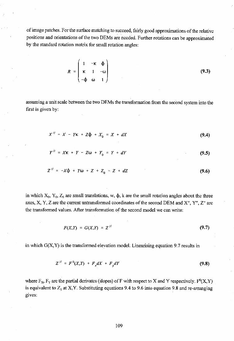
of image patches. For the surface matching.to succeed, fairly good approximations of the relative

positions and orientations of the two DEMs are needed. Further rotations can be approximated

by the standard rotation matrix for small rotation angles:

R = [ ~ -K -~) -cf> w 1

(9.3)

assuming a unit scale between the two DEMs the transformation from the second system into the

first is given by:

X 11 = X - YK + Z<f> + X0

= X + dX

Y 11 = XK + Y - ZW + Y = Y + dY 0

Z 11 = -X<f> + Yw + Z + Z0 = Z + dZ

(9.4)

(9.5)

(9.6)

in which Xo, Y0, Z0 are small translations, w, cf>, k are the small rotation angles about the three

axes, X, Y, Z are the current untransformed coordinates of the second DEM and X", Y", Z" are

the transformed values. After transformation of the secon:d model we can write:

F(X, Y) = G(X, Y) = Z 11 (9.7)

in which G(X, Y) is the transformed elevation model. Linearising equation 9. 7 results in

Z 11 = F 0(X,Y) + F dX + F dY x y (9.8)

where Fx, Fy are the partial derivates (slopes) off with respect to X and Y respectively. F0(X,Y)

is equivalent to Z1 at X,Y. Substituting equations 9.4 to 9.6 into equation 9.8 and re-arranging

gives:

109

Z1 - Z = (F xy - F yK}K + (Y + F yZ>w - (X + F x2)<f> +

- F xKo - F yyo + Zo (9.9)

All the elevation differences Z1 - Z are introduced as observations with associated errors into a

least squares adjustment. The observation equations, in the form v = Ax - 1, are thus given by:

v2 = (FxY -FyK)K + (Y + FyZ)w - (X + Fx2)<f> +

- F xKo - F yYo + Zo - (Zt - Z) (9.10)

After each iteration the second surface is transformed using equations 9.4 to 9.6 and the latest

values X", Y", Z" used in the next iteration. The first DEM is resampled for Zl at each of the

transformed X, Y positions (of second DEM) at the beginning of each iteration. Thus it is easier

to have a regularly spaced grid sampling in the first DEM while the second DEM need not be

regularly sampled. The slopes Fx and F v can be computed in a similar manner to that used for the

least squares matching in images.

A few small tests with simulated data were carried out to test the method. As mentioned by

Karras and Petsa (1993) it was found that even with unperturbed data small residuals remain,

however they did show that approximate orientations between surfaces could be improved upon.

The technique is fairly sensitive to the shapes and spacings of the DEMs as well as to the

provisional values of the transformation parameters, but it still may have potential for the

evaluation of small deformations for some specific surface shapes. As with least squares

matching of images, strong surface gradients in more than one direction and good parameter

approximations are a requirement for reliable and accurate matching.

9.3 INTERACTIVE MATCHING

In many applications only relative positions between a few distinct points on a surface are of

interest. In such cases it becomes unnecessary to measure the whole surface and becomes more

efficient for the operator to interactively measure these points. An option was built into the

system to allow the user to position the reference patch on a point of interest in the one reference

image and the system automatically computes the 3-D coordinates of this point. This is

accomplished by first using the MIC search procedure to compute all provisional conjugate

image positions and space coordinates and then utilising the MPGC matching algorithm to

compute accurate image and object coordinates. The routine then depicts the final image

110

positions of all the patches and also a resampled zoom window of each so that the user can verify

the final results.

Sub-pixel pointing in the reference image is accomplished in a number of ways. The first method

is a manual one which works by displaying an interpolated zoom window of the patch in its sub­

pixel position. A cross hair at the centre of the zoom window allows fine positioning. This

manual method is obviously fairly coarse but does allow for better than one pixel pointing in the

reference image.

The second approach to sub-pixel pointing is as follows. The user positions the patch

approximately, to pixel accuracy. An automatic user selectable function then accurately computes

the sub-pixel position of the reference patch. This function could be template matching (with a

wide variety of template types to choose from, such as circles, corners, edges, crosses, etc.), one

of the centering routines of chapter 6 if the point of interest is circular, intersection of edge

elements for a corner point or any other function that might be needed.

The interactive matching process is considerably strengthened and made more user friendly by

the implementation of the MIC algorithm. Without the MIC procedure, the user would have to

identify the same point in more than one image, which is not always an easy task when the

images are not being viewed as a stereo-pair.

The advantage of having an interactive matching (measuring) capability is that specific

measurements can be quickly made on the surface (or any object) without having to measure the

entire surface. For example the 3-D distance between any two points could be quickly computed,

or a volume, defined by the user selected points, could be easily determined.

111

10. SYSTEM MEASUREMENT TESTS

10.1 PROPELLER SURFACE

The propeller shown in figure 10 .1 provided a complex test surface to measure. It is a good

example of the type of featureless surface that a manufacturer might need to measure, either for

quality control or for reverse engineering.

A special control frame (also seen in figure

10 .'1) was designed for this measurement task.

The frame which was 30x30x10cm in size

was also used for mounting the propeller in an

upright position. The thirty-two 9mm

retroreflective targets were placed in positions

so that all were visible from a camera placed

anywhere between the "extensions" of the

four corners.

The control targets were coordinated by

capturing five images of the frame with one

of the ITC cameras and an 8.5mm lens. A

Figure J 0.1. The propeller and control frame. self-calibrating free network adjustment was

performed to obtain the three dimensional

coordinates of the control points. The first term of radial lens distortion was included in the

adjustment as an unknown additional parameter. The resulting a posteriori standard deviation of

unit weight was 0.0008 and the root mean squares of the object point coordinate standard

deviations were 0.04, 0.04 and 0.09mm for X,Y and Z respectively. The network was scaled by

measuring a single distance between two of the points. The coordinates obtained from this

measurement were used to constrain the exterior orientations for the following surface

measurement stage.

Four images using the same camera were captured of the propeller in the control frame. The

overhead projector and overhead slide with a grid pattern provided the required texture on the

propeller surface. The projector and slide had been switched on for over an hour to warm up. The

projected grid caused a problem with reflected light off the surface, thus the offset, gain and

aperture needed to be carefully fine tuned to obtain useable images. The reflection problem is

caused by the differing angles of the propeller wings and the high reflectance of the metal.

112

A self-calibration adjustment was performed to obtain the interior and exterior orientations of the

images. The resulting a0 from the bundle adjustment was 0.0013 . This value was used as a global

a priori standard deviation for all the collinearity observations in the MPGC matching as

described in section 8.2.4. The a priori standard deviation of all the grey level difference

observations, 01> was obtained from the resulting a 0 from matching a few patches without

constraints (a1 = 3 grey levels was used). The MPGC matching~ blunder level was set to 12

and the maximum iterations to 30. A reference patch size of 9x9 pixels was used for all the

points. A total of 921 points was measured with results as shown in table 10.1.

RMS

Average ax Oy Ox Oy Oz Oo iterations

(pels) (pels) (mm) (mm) (mm)

0.05 0.05 0.04 0.04 0.17 3.8 8.1

Table I 0.1. Results from MPGC matching of propeller surface.

Figure I 0.2. A perspective plot of the propeller surface as produced by the surface

presentation package SURFER.

Of these 921 points, 8 were points extracted outside the surface (but correctly matched) and 50

were marked as outliers of which 34 were inside or on the edge of the central portion, 9 were on

the propeller edge and only 7 on the propeller blade surfaces (as seen from the reference image).

A remaining 13 were not picked up as result outliers but were in fact blunders deduced from their

erroneous heights. Many of the outliers fell in and near the edges of the middle section due to two

reasons, namely the high reflectance of the surface and the steep edges which gave very different

perspective views in the four images. The gross blunders are matched at the wrong local

113

minimum in the images. This happens if the closest point in the DEM image used for the

extrapolation is on a different surface at a height close to an incorrect minimum, as in the case

of the blunders picked up on the propeller. Had the MIC procedure been used before every match

then the chances of this happening would have been greatly reduced, although still possible.

A perspective plot of the cleaned 3-D data is shown in Figure 10.2 with the middle section

blanked out as described in the previous chapter. The display package SURFER used for the

generation of this plot ran out of memory when trying to produce a blanked grid of a higher

density.

10.2 PLASTIC LID

A smooth black plastic lid with a spherical curvature was also measured. A grid was projected

onto the lid using an overhead slide. The control frame used for the propeller measurement was

again used for this measurement project. The projected grid, the lid and the control frame are

depicted in figure 10.3 .

Four images were captured of the surface and

a self-calibrating constrained bundle

adjustment was used for determining the

camera and station parameters. A a0 of 0.0008

was obtained from the bundle adjustment.

The a priori standard deviations of the

observations in the MPGC matching were

globally set to a 1 = 4 grey levels and a 2 = 0.0008mm. The MPGC matching a0 blunder

level was set at 12 and the maximum

iterations to 30. A reference patch size of 9x9

pixels was again used for all the points.

Due to the lid being a smooth and continuous Figure J 0.3. The plastic lid with projected grid. surface the MIC search procedure was only

called for the very first surface point and the extrapolation assumption was adequate for all the

match points on this surface. A much smaller percentage of outliers was detected than for the

propeller. A total of 1252 points was measured with results as shown in table 10.2. Of these

1252 points, 7 were points extracted outside the surface and 29 were outliers of which 26 were

near the edge of the surface. All points, except the seven outside the surface, were used to

generate the perspective grid plot shown in figure 10.4. The majority of outliers fall near the edge

of the surface because the greatest perspective differences occur here.

114

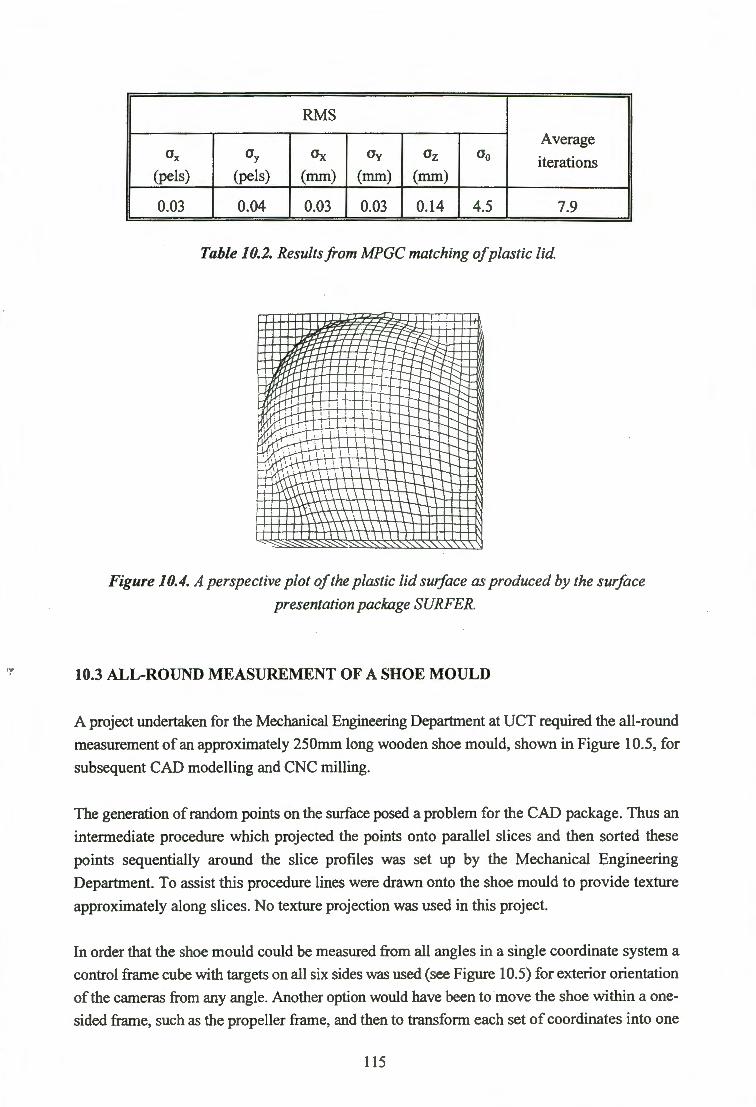
RMS

Average ax Oy Ox Oy Oz Oo iterations

(pels) (pels) (mm) (mm) (mm)

0.03 0.04 0.03 0.03 0.14 4.5 7.9

Table 10.2. Results from MPGC matching of plastic lid

Figure I 0.4. A perspective plot of the plastic lid surface as produced by the surface

presentation package SURFER.

10.3 ALL-ROUND MEASUREMENT OF A SHOE MOULD

A project undertaken for the Mechanical Engineering Department at UCT required the all-round

measurement of an approximately 250mm long wooden shoe mould, shown in Figure 10.5, for

subsequent CAD modelling and CNC milling.

The generation of random points on the surface posed a problem for the CAD package. Thus an

intermediate procedure which projected the points onto parallel slices and then sorted these

points sequentially around the slice profiles was set up by the Mechanical Engineering

Department. To assist this procedure lines were drawn onto the shoe mould to provide texture

approximately along slices. No texture projection was used in this project.

In order that the shoe mould could be measured from all angles in a single coordinate system a

control frame cube with targets on all six sides was used (see Figure 10.5) for exterior orientation

of the cameras from any angle. Another option would have been to move the shoe within a one­

sided frame, such as the propeller frame, and then to transform each set of coordinates into one

115

of the sets using control points on the shoe

surface. The visibility of these control points

from all angles would have posed a difficult

problem so the former option with the all­

round frame was chosen. The frame was

made larger than specified, which resulted in

the image scales being smaller than optimal

for the shoe. A total of 203 retroreflective

targets was attached to the frame. These

targets were coordinated by a self-calibrating

free network adjustment with the scale

provided by a measurement between two of

the targets. Nine images at each face (except

for one face which had eight images) and a Figure 10.5. The wooden shoe mould and

total of32 images to link the faces (total of 85 control frame as seen from the right side.

images) were used in the adjustment. This

resulted in a parameter set of 1129 unknowns which was solvable due to the partitioning scheme

and the DOS extender of Gnu C, although it took about 12 hours to execute on the 486 DX-33

computer. The results of the bundle adjustment are shown in Table 10.3.

df Oo RMS (mm)

ax Oy Oz vx Vy

5660 0.0007 0.039 0.043 0.041 0.0006 0.0006

Table 10.3. Results of the free network adjustment to coordinate the shoe control frame.

As can be seen from the table, the RMS of the standard deviations of the object coordinates

are all of a similar size because the targets as a group have been measured from all sides.

There were quite a few outliers with residuals greater than 3 a0, almost all of which were from

the images used to link the faces. This is due to the oblique view of about 45 degrees to most

of the targets from these image stations. These outliers were left in the data set because of the

high redundancy of the network.

Once the coordinates of the frame had been determined another five images of each side of

the shoe mould were captured. Each side of the mould was measured separately. After

orientating an image set the MPGC matching was performed. After all sets had been

measured in this way their resulting surface coordinates were merged into one result file. Due

116

to the method used by this system for computing provisional values, the coordinate axes of

four of the sides had to be temporarily re-arranged for the processing, to ensure that the Z axis

was always the depth. The algorithms could be modified to allow for this by computing the

general direction of the imaging rays and using the axis with the most depth as the

search/height axis. The average results of all six measurements are shown in table 10.4. Note

that the coordinates given in this table are with respect to the rearranged axes, so that a

comparison can be made (i.e. the Z coordinate is the depth for all six faces).

RMS

Average ox Oy Ox Oy Oz Oo iterations

(pels) (pels) (mm) (mm) (mm)

0.04 0.05 0.04 0.06 0.29 6.0 8.8

Table 10.4. Results from the MPGC matchings of the six sides of the shoe mould. The

average of these six measurements is tabled here.

The results are slightly poorer than for the previous two test surfaces. This can mostly be

attributed to the large perspective differences between the images for the points appearing close

to the surface edge as seen from one or more of the images. The resulting 3-D surface points were

further processed by the Mechanical Engineering Department in AutoCAD. Problems were

encountered with the prioritization of the points, and by the non-uniform spacing and distribution

of the points on the surface. This resulted L.1 a non-uniform mesh which appeared different from

varying angles. Two plots of the interpolated surface grid of the shoe mould are shown in figures

10.6 and 10.7. As can be seen from the profile view, the surface line from the front tip to the high

point is smooth as expected, while from the perspective view this same surface line appears

dented.

Figure 10.6. Profile plot of the shoe mould surface as represented and interpolated by

Auto CAD.

117

Figure 10. 7. Perspective plot of the shoe mould surface as represented and interpolated by

AutoCAD.

This representation and interpolation problem is being further looked at by the Mechanical

Engineering Department. Intermediate software to convert random surface data into evenly

distributed data is needed between the photogrammetric and AutoCAD package.

However, the measurement of the shoe mould showed that all-round surface measurement is

possible with the algorithms described in this thesis. It also showed that different surface texture

(in this case non-projected straightish lines) can be used without any change in the algorithms.

118

11. CONCLUSIONS

The aim of this thesis was to investigate and develop algorithms for an automated surface

measurement system. Some of the characteristics of the system and its algorithms are paraphrased

below. A few recommendations are also given.

The algorithms were integrated specifically for the once-off measurement of general surfaces.

Some additional algorithms for automatic update orientation would be required to make the

system a dedicated measuring device. The algorithms have shown adaptability to the

measurement of different surface types and shapes. In the tests performed in this work, precisions

of less than 5/1 OOth of a millimetre were achieved for the X and Y coordinates of surface points.

Precisions of about 15/lOOth of a millimetre were achieved for the Z (depth) coordinates of

surface points. The measured surfaces were approximately 250mm in the longest dimension, thus

the relative precisions were in the order of 1 :5000 in the plane of the surface and 1: 1700 in the

depth. Obvious improvements in precision would result if more images and higher resolution

cameras (with digital output) were used.

The algorithms are flexible to the type of targeting used. In this work projected grids and hand­

drawn lines have been employed for providing surface detail. Natural texture could also be used.

The only restriction is that the surface detail is fairly dense and of sufficient contrast for

matching. Care has to be taken with the stability of projected targets, unless simultaneous image

capture with multiple cameras is used. It was shown that an off-the-shelf projector and standard

slide did not provide a suitable stability of the projected pattern.

All measurement stages are fully automatic except for the identification of a few control points

for orientation and occasionally some edge editing when determining the surface boundary.

The free network bundle solution offers a flexible method of calibrating cameras without control

points. Thus, time consuming surveys of control point coordinates are not needed and the

network is not constrained to any particular set of points. Good camera calibration is essential

for achieving high accuracies and for reliable matching. Image distortions must be modelled if

significant. In this respect, further research concerning the flatness of sensors is needed.

Extracting artificial targets from images is more reliably accomplished by using a thresholded

gradient (edge) image than by thresholding the grey image. A simple method of finding a

gradient threshold was proposed in this thesis. The best-fitting ellipse routine can be used for the

subsequent identification of circles and ellipses.

119

REFERENCES

Abdel-Aziz, Y.I. and H.M. Karara, 1971. Direct Linear Transformation from Comparator

Coordinates into Object Space Coordinatf!S in Close-Range Photogrammetry,

Proceedings of ASP/UI Symposium ori Close-Range Photogrammetry, Urbana, Illinois,

pp. 1 - 18.

Ackermann, F ., 1984. Digital Image Correlation: Performance and Potential Application in

Photogrammetry, Photogrammetric Record, 11(64), pp. 429 - 439.

Ackermann, F., 1991. Structural Changes in Photogrammetry, Proceedings of the 43rd

Photogrammetric Week, Stuttgart University, September 9 - 14, 1991, pp. 9 - 23.

Ackermann, Fritz and Michael Hahn, 1991. Image Pyramids for Digital Photogrammetry, Digital

Photogrammetric Systems, H. Ebner, D. Fritsch, C. Heipke, Editors, Karlsruhe:

Wichmann, pp. 43 - 58.

Adams, L.P., B. Gutschow, A Tregidga and M. Klein, 1990. Near real time biostereometric

studies of regional body surface motion· in respiration, SPIE Vol. 1395, Close-Range

Photogrammetry Meets Machine Vision, pp. 762 - 767.

Albertz, Jorg and Gerd Konig, 1991. The Advanced Digital Stereophotogrammetric System of

the TU Berlin, Digital Photogrammetric Systems, H. Ebner, D. Fritsch, C. Heipke,

Editors, Karlsruhe: Wichmann, pp. 17 - 27.

Amdal, Knut, Nils Thune and Ole H. Dorum, 1990. Correction of Image Deformations Using

B-Spline Surfaces in Digital Close Range Photogrammetry, SPIE Vol. 1395,

Close-Range Photogrammetry Meets Machine Vision (1990), pp. 845 - 854.

Baltsavias, E.P., 1991. Multiphoto Geometrically Constrained Matching, Dissertation No. 9561,

ETH Zurich.

Baltsavias, Emmanuel P. and Dirk Stallmann,.1990. Trinocular Vision for Automatic and Robust

3-D Determination of the Trajectories of Moving Objects, SPIE Vol. 1395, Close-Range

Photogrammetry Meets Machine Vision, pp. 620 - 629.

122

Beyer, Horst A., 1987. Some Aspects of the Geometric Calibration of CCD-Cameras,

Proceedings of the Intercommision Conference on FastProcessing of Photogramnietric

Data, Interlaken, Switzerland, pp. 68 - 81.

Beyer, Horst A., 1992a. Advances in Characterisation and Calibration of Digital Imaging

Systems, International Archives ofPhotogrammetry and Remote Sensing, Vol. 29, B5,

pp. 545 - 555.

Beyer, Horst A., 1992b.Geometric and Radiometric Analysis of a CCD-Camera Based

Photogrammetric Close-Range System, Dissertation No. 9701, ETH Zurich.

Beyer, Horst A., 1994. Determination of Radiometric and Geometric Characteristics of Frame

Grabbers, International Archives of Photogrammetry and Remote Sensing, Volume 30,

Part 5, pp. 8 - 15.

Beyer, H.A., H.P. Fassler and J. Wen, 1989. Real-Time Photogrammetry in High-Speed Robotics,

Optical 3-D Measurement Techniques, A Gruen, H. Kahmen, Editors, Karlsruhe:

Wichmann, 1989, pp. 271 - 280.

Beyer, H.A. and W. Hoeflinger, 1994. Determination of radiometric and geometric

characteristics of frame grabbers, International Archives of Photogrammetry and Remote

Sensing, Vol. 30, part 5, pp. 8 - 15.

Brown, D.C., 1958. A Solution to the General Problem of Multiple Station Analytical·

Stereotriangulation, RCA Data Reduction Technical Report No. 43.

Brown, D.C., 1971. Close-Range Camera Calibration, Photogrammetric Engineering, 37(8), pp.

855 - 866.

Brown, Duane C., 1980. Application of Close-Range Photogrammetry to Measurements of

Structures in Orbit, Volume 1, GSI Technical Report No. 80-012.

Burner, A.W., W.L. Snow, M.R. Shortis and W.K. Goad, 1990. Laboratory Calibration and

Characterization of Video Cameras, SPIE Vol. 1395, Close-Range Photogrammetry

Meets Machine Vision (1990), pp. 664 - 671.

Canny, John, 1986. A Computational Approach to Edge Detection, IEEE Transactions on Pattern

Analysis and Machine Intelligence, Vol. PAMI-8, No. 6, pp~ 679 - 698.

123

Clarke, T.A., M.A.R. Cooper, J. Chen and S. Robson, 1994. Automated 3-D Measurement Using

Multiple CCD Camera Views, Photogrammetric Record, In Press (presented at Thompson

Symposium, York, England).

Claus, Michael, 1984. Digital Terrain Models Through Digital Stereo Correlation,

Photogrammetria, 39, pp.183-192.

Cogan, Louis, Thomas Luhmann and A. Stewart Walker, 1991. Digital Photogrammetry at

Leica, Aarau, Digital Photogrammetric Systems, H. Ebner, D. Fritsch, C. Heipke,

Editors, Karlsruhe: Wichmann, pp. 155 - 166.

Dahler, J., 1987. Problems in Digital Image Acquisition with CCD Cameras, Proceedings of the

Intercommission Conference on Fast Processing of Photogrammetric Data, Interlaken,

Switzerland, pp. 48 - 59.

Dermanis, Athanasios, 1994. The Photogrammetric Inner Constraints, ISPRS Journal of

Photogrammetry and Remote Sensing, 49(1), pp. 25 - 39.

Dold, Jurgen and Hans-Gerd Maas, 1994. An application of epipolar line intersection in a hybrid

close range photogrammetric system, International Archives of Photogrammetry and

Remote Sensing, Vol. 30, Part 5, pp. 65 - 70.

Dowman, I.J., 1984. Problems and Some Solutions in Digital Correlation for Photogrammetric

Profiling, Photogrammetria, 39, pp.155-167.

El-Hakim, S.F., 1984. A Photogrammetric Vision System for Robots, Internationa! Archives of

Photogrammetry and Remote Sensing, Vol 25, Part AS, pp. 223 - 231.

El-Hakim, S.F., 1986. Real-Time Image Metrology with CCD Cameras, Photogrammetric

Engineering and Remote Sensing, Vol. 52, No. 11, pp. 1757 - 1766.

El-Hakim, Sabry F., 1990. Some Solutions to Vision Dimensional Metrology Problems, SPIE

Vol. 1395, Close-Range Photogrammetry Meets Machine Vision (1990), pp. 480 - 487.

El-Hakim, S.F., and M.A. Barakat, 1989. A Vision-Based Coordinate Measuring Machine

· (VCMM), Optical 3-D Measurement Techniques, A. Gruen, H. Kahmen, Editors,

Karlsruhe: Wichmann, 1989, pp. 216 - 228.

Forstner, W. and E. Gulch, 1987. A Fast Operator for Detection and Precise Location of Distinct

Points, Corners and Centres of Circular Features, Proceedings of the Intercommission

124

Conference on Fast Processing of Photogrammetric Data, Interlaken, Switzerland, June

2 - 4, 1987, pp. 281 - 305.

Fraser, C. S., 1982. Optimization of Precision in Close-Range Photogrammetry,

Photogrammetric Engineering and Remote Sensing, Vol. 48, No. 4, pp. 561-570.

Fraser, Clive S., 1987. Limiting Versus Total Error Propagation, presented at the International

Colloquium on Network Design Optimization in Non-Topographic Photogrammetry,

ISPRS WG V/1, Baltimore, Maryland, 10 pages.

Fraser, Clive, S., 1992. Photogrammetric Measurement to One Part in a Million,

Photogrammetric Engineering and Remote Sensing, 58(3), pp. 305 - 310.

Fritsch, D., 1989. Algorithms in Fast Vision Systems, Optical 3-D Measurement Techniques, A.

Gruen, H. Kahmen, Editors, Karlsruhe: Wichmann, pp. 87 - 102.

Frobin, W. and E. Hierholzer, 1985. Simplified Rasterstereography Using a Metric Camera,

Photogrammetric Engineering and Remote Sensing, Vol. 51, No. 10, pp. 1605 - 1608.

Fryer, John G., 1989. Camera Calibration in Non-Topographic Photogrammetry, NON­

TOPOGRAPHIC PHOTOGRAMMETRY, Second Edition, Editor: H. M. Karara,

American Society for Photogrammetry and Remote Sensing, pp. 59 - 69.

Fryer, John G. and Duane C. Brown, 1986. Lens Distortion for Close-Range Photogrammetry,

Photogrammetric Engineering and Remote Sensing, Vol. 52, No. 1, pp. 51 - 58.

Godding, Robert, 1990. A System for the Photogrammetric Evaluation of Digitized High-Spe,ed

Images in the Automobile Industry, SPIE Vol. 1395, Close-Range Photogrammetry Meets

Machine Vision (1990), pp. 314 - 319.

Godding, Robert and Thomas Luhmann, 1992. Calibration and Accuracy Assessment of a

Multi-Sensor Online-Photogrammetric System, International Archives · of

Photogrammetry and Remote Sensing, Vol. 29, B5, pp. 24 - 29.

Granshaw, S. I., 1980. Bundle Adjustment Methods in Engineering Photogrammetry,

Photogrammetric Record, 10(56), pp.181 - 207.

Grun, Armin, 1978. Accuracy, Reliability and Statistics in Close-Range Photogrammetry,

Presented paper, Inter-Congress Symposium, Commission V, International Society for

Photogrammetry, Stockholm.

125

Gruen, A.W., 1985. Adaptive Least Squares Correlation: A Powerful Image Matching

Technique, South African Journal of Photogrammetry, Remote Sensing and Cartography,

14(3), 1985, pp. 175 -187.

Gruen, Armin, 1994. Digital Close-Range Photogrammetry - Progress Through Automation,

International Archives of Photogrammetry and Remote Sensing, Vol. 30, Part 5, pp. 122

- 135.

Gruen, Armin and Emmanuel Baltsavias, 1988. Automatic 3-D Measurement of Human Faces

with CCD-Cameras, SPIE Vol. 1030, Biostereometrics (1988), pp. 106 - 116.

Gruen, Armin W. and Horst A. Beyer, 1987. Real-Time Photogrammetry at the Digital

Photogrammetric Station (DIPS) of ETH Zurich, The Canadian Surveyor, Vol. 41, No.

2, pp. 181 - 199.

Gruen, Armin and Horst A. Beyer, 1991. DIPS II - Turning a Standard Computer Workstation

into a Digital Photogrammetric Station, ZPF - Zeitschrift fur Photogrammetrie und

Fernerkundung; pp. 2 - 10.

Gustafson, Peter C. and Harry B. Handley, 1992. A Video-Based Industrial Measurement

System, International Archives of Photogrammetry and Remote Sensing, Vol. 29, B5, pp.

501 - 506.

Haggren, Henrik, 1984. New Vistas for Industrial Photogrammetry, International Archives of

Photogrammetry and Remote Sensing, Vol 25, Part A5, pp. 382 - 391.

Haggren, Henrik, 1987. Real-Time Photogrammetry as used for Machine Vision Applications,

The Canadian Surveyor, Vol. 41, No. 2, pp. 201 - 208.

~

Haggren, Henrik, 1989. Photogrammetric Machine Vision, Optics and Lasers in Engineering, 10,

pp. 265 - 286.

Haggren, H., 1991. Real-Time Photogrammetry and Robot Vision, Proceedings of the 43rd

Photogrammetric Week, Stuttgart University, September 9 - 14, 1991, pp. 245 - 251.

Haggren, Henrik and Esa Leikas, 1987. MAP VISION - The Photogrammetric Machine Vision

System, Proceedings of the Intercommission Conference on Fast Processing of

Photogrammetric Data, Interlaken, Switzerland, pp. 350 - 362.

126

Haggren, Henrik and Leif Haajanen, 1990. Target Search Using Template Images, SPIE Vol.

1395, Close-Range Photogrammetry Meets Machine Vision, pp. 572 - 578.

Heikkila, Jan, 1990. Update Calibration of a Photogrammetric Station, SPIE Vol. 1395, Close­

Range Photogrammetry Meets Machine Vision, pp. 1234 - 1241.

Heipke, C., M. Stephani, G. Strunz and R. Lenz, 1992. Photogrammetric Calibration and Point

Determination Using a Digital CCD Camera, International Archives of Photogrammetry

and Remote Sensing, Vol. 29, B5, pp. 556 - 560.

Heipke, C., P. Saisi and M. Stephani, 1994. Art Inventarisation and Preservation by Digital

Photogrammetry, International Archives of Photogrammetry and Remote Sensing, Vol.

30, Part 5, pp. 171 - 177.

Hinsken, Ludger, 1988. A Singularity Free Algorithm for Spatial Orientation of Bundles,

International Archives of Photogrammetry and Remote Sensing, Vol. 27, B5, pp. 262 -

272.

Huang, Y. and J.C. Trinder, 1993. A Procedure for Fully Automatic Orientation of Camera in

Digital Close Range Photogrammetry, Optical 3-D Measurement Techniques, A. Gruen,

H. Kahmen, Editors, Karlsruhe: Wichmann, pp. 339 - 346.

Huertas, Andres and Gerard Medioni, 1986. Detection of Intensity Changes with Subpixel

Accuracy Using Laplacian-Gaussian Masks, IEEE Transactions on Pattern Analysis and

Machine Intelligence, Vol. PAMI-8, No. 5, pp. 651 - 664.

Jeschke, Wolfgang, 1990. Digital Close-Range Photogrammetry for Surface Measurement, SPIE

Vol. 1395, Close-Range Photogrammetry Meets Machine Vision (1990), pp. 1058 - 1065.

Kaiser, Richard, 1991. The Intergraph Digital Photogrammetric Workstation, Proceedings of the

43rd Photogrammetric Week, Stuttgart University, September 9- 14, 1991, pp. 195 - 202.

Karras, George E. and Elli Petsa, 1993. DEM Matching and Detection of Deformation in Close­

Range Photogrammetry without Control, Photogrammetric Engineering and Remote

Sensing, Vol. 59, No. 9, pp. 1419 - 1424.

Krzystek, P ., 1991. Fully Automatic Measurement of Digital Elevation Models with MA TCH-T,

Proceedings of the 43rd Photogrammetric Week, Stuttgart University, September 9 - 14,

1991, pp. 203 - 214.

127

Lenz, Reimar, 1989. Image Data Acquisition with CCD Cameras, Optical 3-D Measurement

Techniques, A. Gruen, H. Kahmen, Editors, Karlsruhe: Wichmann, pp. 23 - 34.

Lenz, Reimar, Roland Beutlhauser and Udo Lenz, 1994. A Microscan I Macroscan 3 x 12 Bit

Digital Color CCD Camera with Programmable Resolution up to 20992 x 20480 Picture

Elements, International Archives of Photogrammetry and Remote Sensing, Vol. 30, Part

5, pp. 225 - 230.

Lenz, Reimar and Dieter Fritsch, 1990. Accuracy of Videometry with CCD Sensors, ISPRS

Journal of Photogrammetry and Remote Sensing, 45, pp. 90 - 110.

Lenz, R. and U. Lenz, 1993. New Developments in High Resolution Image Acquisition with

CCD Area Sensors, Optical 3-D Measurement Techniques, A. Gruen, H. Kahmen,

Editors, Karlsruhe: Wichmann, 1993, pp. 53 - 62.

Lim, Jae S., 1984. Image Enhancement, DIGITAL IMAGE PROCESSING TECHNIQUES,

Editor: Michael P. Ekstrom, Academic Press Inc., Florida, pp. 1 - 51.

Luhmann, Thomas, 1990a. Image Recording Systems for Close-Range Photogrammetry, SPIE

Vol. 1395, Close-Range Photogrammetry Meets Machine Vision (1990), pp. 86 - 95.

Luhmann, Thomas, 1990b. An Integrated System for Real-Time and On-Line Applications in

Industrial Photogrammetry, SPIE Vol. 1395, Close..:Range Photogrammetry Meets

Machine Vision (1990), pp. 488 - 495.

Luhmann, Thomas and Wilfried Wester-Ebbirtghaus, 1987. On Geometric Calibration of

Digitized Video Images ofCCD Arrays, Proceedings of the Intercommission Conference

on Fast Processing of Photogrammetric Data, Interlaken, Switzerland, June 2-4, 1987, pp.

35 - 47.

Maas Hans-Gerd, 1990. Digital Photogrammetry for Determination of Tracer Particle

Coordinates in Turbulent Flow Research, SPIE Vol. 1395, Close-Range Photogrammetzy

Meets Machine Vision, pp. 391 - 398.

Maas, Hans-Gerd, 1992a. High-Speed Solid State Camera Systems for Digital Photogrammetry,

International Archives of Photogrammetry and Remote Sensing, Vol. 29, BS, pp. 482 -

485.

128

Maas, Hans-Gerd, 1992b. Robust Automatic Surface Reconstruction with Structured Light,

International Archives of Photogrammetry and Remote Sensing, Vol. 29, B5, pp. 709 -

713.

Maclean, S.G., M. Rioux, F. Blais, J. Grodski, P. Milgram, H.F.L. Pinkney and B.A. Aikenhead,

1990. Vision System Development in a Space Simulation Laboratory, SPIE Vol. 1395,

Close-Range Photogrammetry Meets Machine Vision (1990), pp. 8 - 15.

Magee, M.J. and J.K. Aggarwal, 1985. Using Multisensory Images to Derive the Structure of

Three-Dimensional Objects - A Review, Computer Vision, Graphics, and Image

Processing, 32, pp 145 - 157.

Mayr, W., 1991. PH/PS -A New Tool for Digital Photogrammetry, Proceedings of the 43rd

Photogrammetric Week, Stuttgart University, September 9 - 14, 1991, pp. 31 - 35.

Mikhail, Edward M., Mark L. Akey and O.R. Mitchell, 1984. Detection and Sub-Pixel Location

of Photogrammetric Targets in Digital Images, Photogrammetria, 39, pp. 63 - 83.

Mitchell, H.L., 1994. A Comprehensive System for Automated Body Surface Measurement,

International Archives of Photogrammetry and Remote Sensing, vol. 30, part 5, pp. 265 -

272.

Peipe, J.,C.-Th. Schneider and K. Sinnreich, 1993. Digital Photogrammetric Station DPA -A

Measurement System for Close-Range Photogrammetry, Optical 3-D Measurement

Techniques, A. Gruen, H. Kahmen, Editors, Karlsruhe: Wichmann, 1993, pp. 292 - 300.

Peipe, Jurgen, Carl-Thomas Schneider and Kurt Sinnreich, 1994. Performance of a PC Based

Digital Photogrammetric Station, International Archives of Photogrammetry and Remote

Sensing, Vol. 30, part 5, pp. 304 - 309.

Pettersen, Alf, 1992. Metrology Norway System - Optimum Accuracy Based on CCD Cameras,

International Archives of Photogrammetry and Remote Sensing, Vol. 29, B5, pp. 230 -

233.

Raynor, J.M. and P. Seitz, 1990. The Technology and Practical Problems of Pixel-Synchronous

CCD Data Acquisition for Optical Metrology Applications, SPIE Vol. 13 95, Close-Range

Photogrammetry Meets Machine Vision, pp. 96 - 103.

Rosenfeld, Azriel and Larry S. Davis, 1976. A Note on Thinning, IEEE Transactions on Systems,

Man, and Cybernetics, March 1976.

129

Rosenholm, D., 1987. Least Squares Matching Method: Some Experimental Results,

Photogramrnetric Record, 12(70), pp. 493 - 512.

Rosenholm, Dan and Kennert Torlegard,\ 1988. Three-Dimensional Absolute Orientation of

Stereo ·Models Using Digital Elevation Models, Photograrnmetric. Engineering and

Remote Sensing, Vol. 54, No. 10, pp. 1385 - 1389.

Rubinstein, M., 1990. Assessing Target Centring Algorithms for use in Near-Real-Time­

Photogrammetry, unpublished MSc thesis, University of Cape Town.

Ruther, H. and N. Parkyn, 1990. Near Real Time Photogrammetry on a Personal Computer,

Photogrammetric Record, 13(75), pp. 413 - 420.

Ruther, H. and R. Wildschek, 1989. Digital Photogrammetryfor the Acquisition of Surface Data

for Automatic Milling Processes, Optical 3-D Measurement Techniques, A. Gruen, H.

Kahmen, Editors, Karlsruhe: Wichmann, 1989, pp. 360 - 369.

Sarkar, Sudeep and Kim L. Boyer, 1991. On Optimal Infinite Impulse Response Edge Detection

Filters, IEEE Transactions on Pattern Analysis and Machine Intelligence, Vol. 13, No.

11, pp. 1154- 1171.

Schneider, Carl-Thomas and Kurt Sinnreich, 1990. Concept of an Optical Coordinate

MeasurementMachine, SPIE Vol. 1395, Close-Range Photograrnmetry Meets Machine

Vision (1990), pp. 816 - 822.

Schneider, Carl-Thomas and Kurt Sinnreich, 1992. Optical 3-D Measurement Systems for

Quality Control in Industry, International Archives of Photograrnmetry and Remote

Sensing, Vol. 29, BS, pp. 56 - 59.

Stahs, T.G. and F.M. Wahl, 1990. Fast and Robust Range Data Acquisition in a Low-Cost . .•· . 11

Environment, SPIE Vol. 1395, Close-Range Photograrnmetry Meets Machine Vision

(1990), pp. 496 - 503. .

Tabatabai, Ali J. and 0. Robert Mitchell, 1984. Edge Location to Subpixel Values in Digital

Imagery, IEEE Transactions on Pattern Analysis and Machine Intelligence, Vol. P AMI-6,

No. 2, pp. 188 - 201.

Thompson, E. H., 1969. AN INTRODUCTION TO THE ALGEBRA OF MATRICES WITM

SOME APPLICATIONS, Adam Hilger LTD London.

130

Tiziani, H., 1989. Optical 3-D Measurement Techniques - a Survey, Optical 3-D Measurement

Techniques, A. Gruen, H. Kahmen, Editors, Karlsruhe: Wichmann, 1989, pp. 3 - 21.

Tiziani, H.J., 1993. High Resolution Optical Surface Topography Measurements, Optical 3-D

Measurement Techniques, A. Gruen, H. Kahmen, Editors, Karlsruhe: Wichmann, 1993,

pp. 23 - 32.

Torlegard, K., 1981. Accuracy Improvements in Close Range Photogrammetry, Schriftenreihe,

HSBw, Studiengang Vermessungswesen, Hochschule der Bundeswehr Munchen.

Trinder, J.C., 1989. Precision of Digital Target Location, Photogrammetric Engineering and

Remote Sensing, Vol. SS, No. 6, pp. 883 - 886.

Trinder, J.C., T. Tjugiarto and B.E. Donnelly, 1990. A Close Range Digital Photogrammetry

System, SPIE Vol. 139S, Close-Range Photogrammetry Meets Machine Vision (1990),

pp. 440 - 447.

Turner-Smith, Alan R. and J. Derek Harris, 1986. Measurement and Analysis of Human Back

Surface Shape, International Archives of Photogrammetry and Remote Sensing, Vol. 26,

S, pp. 3SS - 362.

Van den Heuvel, F.A., 1993. Automated 3-D Measurement with the DCS200 digital camera,

Optical 3-D Measurement Techniques, A Gruen, H. Kahmen, Editors, Karlsruhe:

Wichmann, 1993, pp. 63 - 71.

Van den Heuvel, F.A. and R.J.G.A. Kroon, 1992. Digital Close-Range Photogrammetry Using

Artificial Targets, International Archives of Photogrammetry and Remote Sensing, Vol.

29, BS, pp. 222 - 229.

Van der Merwe, Nick and Heinz Ruther, 1994. Image Matching Through a Combination of

Feature and Area Based Matching, International Archives of Photogrammetry and

Remote Sensing, Vol. 30, part S, pp. 407 - 413.

Van der Vlugt, G. and H. Ruther, 1992. A Real-Time Photogrammetric System for Patient

Positioning in Proton Therapy, International Archives of Photogrammetry and Remote

Sensing, Vol 29, BS, pp. 880 - 884.

VanderVlugt, G. andH. Ruther, 1994. The DevelopmentofanAutomatedSurface Measurement

System, International Archives of Photogrammetry and Remote Sensing, Vol. 30, part S,

pp. 414 - 419.

131

Vollmerhaus, Dieter, 1987. A Fast Algorithm for Local Matching of Patterns in Images,

Proceedings of the Intercomission Conference on Fast Processing of Photogrammetric

Data, Interlaken,, Switzerland, June 2 - 4, 1987, pp. 273 - 280.

Wang, Y.F., A. Mitchie and J.K. Aggarwal, 1987. Computation of Surface Orientation and

Structure of Objects Using Grid Coding, IEEE Transactions on Pattern Analysis and

Macine Intelligence, Vol. PAMI-9, No. 1, pp. 129 - 137.

Wehr, A. and M. Ioannides, 1993. Volume reconstruction by using 4-D object surface data,

Optical 3-D Measurement Techniques, A. Gruen, H. Kahmen, Editors, Karlsruhe:

Wichmann, 1993, pp. 33 - 40.

Wiley, Anthony G. and Kam W. Wong, 1990. Metric Aspects of Zoom Vision, SPIE Vol. 1395,

Close-Range Photogrammetry Meets Machine Vision (1990), pp. 112 - 118.

Wilson, R. and F. Leberl, 1990. Real-Time Close-Range 3-D Non-Contact Volume and Motion

Measurements, SPIE Vol. 1395, Close-Range Photogrammetry Meets Machine Vision

(1990), pp. 24 - 29.

Wong, Kam W. and Wei-Hsin Ho, 1986. Close-Range Mapping with a Solid State Camera,

Photogrammetric Engineering and Remote Sensing, Vol. 52, No. 1, pp. 67 - 74.

Wong, Kam W., Ying Ke, Mary Slaughter and Randall Gretebeck, 1992. A Computer Vision

System for Mapping Human Bodies, International Archives of Photogrammetry and

Remote Sensing, Vol. 29, B5, pp. 850 - 855.

Wong, Kam W., Michael Lew and Ying Ke, 1990. Experience with Two Vision Systems, SPIE

Vol. 1395, Close-Range Photogrammetry Meets Machine Vision (1990), pp. 3 - 7.

Wrobel, Bernard, P., 1991. Least-Squares Methods for Surface Reconstruction.from Images,

ISPRS Journal of Photogrammetry and Remote Sensing, 46, pp. 67 - 84.

Zhou, H.B., 1990. Object Points Detection in a Photogrammetric Test Field, SPIE Vol. 1395,

Close-Range Photogrammetry Meets Machine Vision, pp. 1227 - 1233.

132