7- 1

Design Principles and Algorithms for Automated Air Traffic Management

Heinz Erzberger NASA Ames Research Center

MS 210-9, Moffett Federal Airfield

USA CA 94035-1000

Albstract This paper presents design principles and algorithm for building a real time scheduler. The primary objective of the scheduler is to assign arrival aircraft to a favorable landing runway and schedule them to land at times that minimize delays. A further objective of the scheduler is to allocate delays between high altitude airspace for from the airport and low altitude airspace near the airport. A method of delay allocation is described that minimizes the average operating cost in the presence of errors in controlling - aircraft to a specified landing time.

INTRODUCTION The urgent need for increasing the efficiency of'the air traffic management process has led to intense efforts in designing automation systems for air traffic control. The efforts have been dominated by two major technical c h a1 1 en g e s : a t r a j e c tory synthesizer/estimator and a real time scheduler. The design of the trajectory syn thesizer/es tim ator, though technically complex, can be accomplished by the application of well established methods for navigation, guidance and control of aircraft [l], [2]. In contrast, the design of the real time scheduler has no technical precedence to build upon and has been found to require a unique blend of expert knowledge of air traffic control and analytical procedures. It is therefore an especially appropriate subject for this lecture series.

de si g n i n g

The scheduler described herein is incorporated in the Center TRACON Automation System (CTAS) which is being de.veloped jointly by NASA Ames Research Center and the Federal Aviation Administration. The automation tools in CTAS consist of the Traffic Management Advisor, (TMA) the Descent Advisor (DA) and the Final Approach Spacing Tool (FAST) [3]-[5]. These tools generate advisories that assist controllers in handling aircraft from about 40 minutes of flying time to an airport, until they reach the final approach fix. While the design of CTAS is

not yet complete, several of its tools have undergone extensive real time simulation tests as well as field evaluation at the Denver and DallasEort Worth airports [6]-[8].

ROUTE STRUCTURE AND SCHEDULING CONSTRAINTS The basic objective of the scheduler in air traffic control automation is to match traffic demand and airport capacity while minimizing delays. As we shall see, this concise and straight forward sounding objective gives rise to a surprisingly complex algorithmic design problem when all necessary operational constraints are considered. In this chapter we present an outline of the solution to this problem.

The dynamic nature of air traffic flow requires that the scheduler be designed to operate as a real time process which is defined in the following way. The scheduler must generate an updated schedule for the set of aircraft to be scheduled both periodically and in response to aperiodic events. The length of the periodic cycle is related to the basic radar update rate, which is 10-12 seconds in length. In Center airspace, experience has shown the scheduler update cycle must be a small multiple of the radar update cycle, or in the range of 30-60 seconds. Aperiodic events requiring an immediate update of the -schedule are primarily due to controller inputs such as a

Paper presented at the Mission Systems Panel of AGARD and the Consultant and Exchange Program of AGARD held in Madrid, Spain, on 6-7 November 1995; ChBtillon, France, 9-10 November 1995;

and NASA AMES Research Centre, California, USA, 16-17 November 1995 and published in LS-200.

7-2

change in airport configuration, a change in airport landing capacity, etc. While controllers prefer a nearly instantaneous response of the scheduler to such inputs, in practice a response within 10-15 seconds has been found to be acceptable and qualifies as real time performance.

The objective of minimizing delays implies that mathematical optimization must be performed by the scheduler in real time. However, it is recognized that an algorithmic solution of the full scheduling optimization problem with all important constraints included is infeasible and probably impossible. In light of this situation, numerous studies have been done to synthesize practical algorithms that combine both adequate scheduling efficiency and short computation times, so as to maintain real time performance.

The scheduling principle underlying all practical real time scheduling algorithms that have so far been developed is referred to as first-come-first-served (FCFS) [3], [9]. In general, this principle generates "fair" schedules when delays must be absorbed. It is also known to be an optimum schedule for a simple constraint condition and performance criterion. In the discussions to follow, this principle is therefore the starting point for important aspects of the scheduler design. A precise definition of FCFS in the context of air traffic scheduling will be given later.

In addition to the FCFS principle, the scheduling problem is characterized by numerous constraints. The complexity of the scheduling algorithm that remains true to the FCFS principle is greatly increased by the presence of these constraints, as will be seen when the algorithm is derived.

Nevertheless the scheduling algorithm described herein generates a feasible FCFS schedule without computationally lengthy iterative procedures, thereby achieving the precondition for real time operation.

Airspace and Route Structure In order to serve the changing needs of airlines and air traffic control, the airspace and route structure surrounding a large airport have evolved into increasingly complex forms. Here we describe only those features that relate directly to the design of the scheduler. For the purpose of the scheduler design, the arrival airspace is divided into Center and TRACON regions. Whereas the Center region has an irregular outer boundary, the TRACON region is a roughly circular area about 35 n.ni. in radius and is completely surrounded by the Center airspace. Certain way points located on the boundary between the two regions are referred to as meter gates. During moderate and heavy traffic conditions when delays are expected, traffic is funneled through these gates as a means of controlling or metering the flow rate into the terminal area. In most terminal areas, arrival routes are merged at four gates corresponding to the primary arrival directions. An exception is the terminal area for the new Denver International Airport, where eight primary gates, grouped into four closely spaced pairs, are in use.

Traffic flowing to each gate is often segregated into two independent streams by separating each stream vertically by at least 2000 feet in altitude at the gate crossing point. This is done so as to permit the two primary aircraft types, jets and turboprops, which have significantly different airspeed ranges, to cross the gates independently, thereby avoiding conflicts due to overtakes near the gates.

From each gate, routes are defined in the TRACON airspace that lead to all possible landing runways for each independent stream. For the design of the scheduler, the exact horizontal path of the routes is not important; only the nominal flying times from each gate to all landing runways must be provided as input. Figure 1 illustrates the concepts of airspace structure, arrival routes, meter gates and stream types as has been described above.

7-3

Scheduling Constraints: In-Trail Distance Separations Scheduling constraints can be broadly classified into two types: In trail distance separation constraints and sequence order constraints. Here the former is discussed.

In the design of the scheduling algorithm, the in-trail constraints play an especially important role because they determine the capacity of an airport and hence the maximum landing rate. The scheduling algorithm must be designed to meet in-trail constraints both at the meter gates and on the final approach paths.

At the meter gates in-trail separations may be specified by separate parameters for each independent traffic stream in order to provide flexible control of the total flow rate into the TRACON. However, in the absence of flow rate control at the meter gates, safety considerations require the minimum in-trail distance separations to be not less than 5 n.m. Since scheduling is done in the time domain all distances must be converted into equivalent time separations. In general, the conversion first determines the ground speed from estimates of airspeed and wind speed and then applies the following relation:

(1) Ti, = Di, I Vg

where: Dit = specified in-trail distance separation V g = estimated ground speed of trailing

aircraft Ti, = time separation of trailing aircraft from

leading aircraft when leading aircraft is at time control point

This relation not withstanding, a fixed value of one minute for the minimum time separation has been found to be adequate and is used throughout this paper.

On the final approach path the minimum in- trail distance separations are a function of both aircraft weight class and landing order as determined by the FAA's wake vortex safety rules. Table 1 gives the values in matrix format.

The table also gives examples of aircraft models falling in the different weight categories. A separate classification exists for "small," aircraft having landing weights below 12,500 lbs. Such aircraft do not contribute a large fraction of traffic at hub airports and therefore are not included. They could be included in Table 1 by adding a fourth row and column.

As before, the distance separation in Table 1 must be converted to equivalent time separation for use by the scheduler. The conversion process is complex and is given here only in outline. Generally it involves modeling the airspeed profile of each type of aircraft and the wind speed on final approach and then integrating the equations of motion along the final approach path. The result of this process is the time separation matrix given in Table 2 for the case of zero wind.

Scheduling Constraints: Sequence Order and the Definition of First-Come-First- Served A sequence order constraint specifies the order with respect to time that a group of aircraft must be scheduled to cross a time control point. The runway threshold and the meter gates are the points where sequence constraints are frequently enforced. They provide an essential mechanism for achieving scheduling efficiency, scheduling fairness and controller preference. The sequence order that often meets the requirements of all three of these objectives simultaneously is the First-Come-First- Served (FCFS) order. It therefore plays the role of the standard or canonical sequence order against which all other orders are referenced.

Let (ETA(i))N be the set of estimated times of arrival for the set of N aircraft ( A j ) N at the runway threshold, where the Ai are the aircraft identifiers. Then the FCFS order at this point is the time-ordered list of this set of ETA'S arranged in a vertical column, as shown in Table 3.

By convention and for economy of notation the earliest ETA at the bottom of the list is associated with aircraft AI , while the latest ETA at the top is associated with aircraft AN.

Table 1 : Minimum distance separation matrix for pairs of aircraft simultaneously on final approach path, n.m.

Trailing Heavy Trailing Large Trailing Large Jet Jet Tu r bo p ro p

Lead Aircraft Heavy Jet 4.0 5.0 5.0

Lead Aircraft Large Jet 2.5 2.5 2.5

Lead Aircraft Large 2.5 2.5 2.5

(747, DC-10)

(MD 80,737)

Turboprop (AT 42, King Air) .

Trailing Heavy Trailing Large Trailing Large Jet Jet Turboprop

Leading Heavy 113 135 170 Jet

Jet

Turbo prop

Leading Large 89 89 110

Leading Large a3 83 94

Table 2: Minimum time separation matrix for pairs of aircraft on final approach, seconds

.

Table 3: FCFS Ordered List of ETA'S Table 4: Illustration of Position-Shifted Sequence Order relative to FCFS order

ETA (A,) (latest) FCFS Postiton Shifted Orde r

ETA(A,,,)- A,,,

ETA ( A , ) - AI

A sequence list of aircraft not in FCFS order is said to be position-shifted. A position- shifted order can be displayed graphically by placing the FCFS order list of ETA's and the position-shifted list of aircraft identifiers adjacent to each other and then connecting corresponding ETA's and aircraft identifiers with lines as shown in Table 4.

The crossed lines identify the aircraft that are position-shifted. In Table 4, A2 and A3 are position-shifted by one, meaning that an order reversal of these two adjacent aircraft returns them to FCFS order. Higher order position-shifts would appear as multiple line crossings. If advancing an aircraft by k slots relative to FCFS is defined as a positive position shift of k and delaying it by 1 slots is defined as a negative position-shift of 1, then it can be shown that the algebraic sum of all position shifts of an arbitrarily position- shifted sequence order is zero.

The basic sequence order constraints for which the scheduling algorithm will be derived consist of FCFS order at the runway and FCFS order for each independent stream at each meter gate.

The algorithm can easily be adapted to accommodate position-shifted sequence order at the runway or the meter gates. Position shifting is a technique for reducing delays by optimizing the landing sequence and will be discussed later.

Recently, Brinton developed an algorithm for sequence and runway assignment optimization using a variant of binary enumeration and branch and bound technique [lo].

DESCRIPTION OF THE BASIC ALGORITHM In this section the basic algorithm that generates schedules to the runway threshold while obeying FCFS sequence constraints at both meter gates and runways is described. 'The algorithm builds the schedule by a non- iterative constructive procedure that translates directly into a rapidly executing software program. While the algorithm

packs aircraft as tightly together as the constraints permit, it does not optimize any specific performance functions. If sufficient computing power and time are available, the schedule generated by the basic algorithm, can, however, serve as the initial schedule for iterative algorithms, such as described in [lo], that reduce delays by optimizing the landing sequence and runway allocations. The next chapter describes an optimization approach that works within real time constraints.

It is assumed that the schedulable aircraft are in Center airspace and some distance away from the meter gate. The basic input to the scheduler is the set of estimated times of arrival of all schedulable aircraft, computed to the appropriate meter gates. This set, designated by {ETAFF} i s provided by the trajectory synthesizer algorithm. For the sake of simplicity but without loss of generality, the derivation is given for the case of two meter gates, A and B, and one runway. Aircraft assigned to these gates have associated identifiers {A,},and {B,}N, respectively.

Thus M+N are the total number of aircraft to be scheduled. Let ( T l ( A i ) } , and {T,(13,)}N be the set of TRACON transition times. They specify the nominal time intervals required for aircraft to fly from their respective meter gates, A or B, to the runway threshold. Therefore, the estimated time of arrival of aircraft A i at the threshold can be written as ETA(Ai) =ETAFF(Ai)+Tr(Ai), and similarly for aircraft B,. The set of transition times are input quantities also generated by the trajectory synthesis algorithm.

A series of time lines will be used to illustrate various steps in the development of the scheduling algorithm. Each figure in the series consists of several vertical time lines arranged side by side representing a geographic scheduling point, either a meter gate or a runway. The transformation and procedures described in the various steps are

7-6

represented graphically by lines connecting objects on adjacent time lines. The objects are generally the aircraft to be scheduled. By studying the figures in sequence the reader can follow a specific scheduling problem from beginning to end.

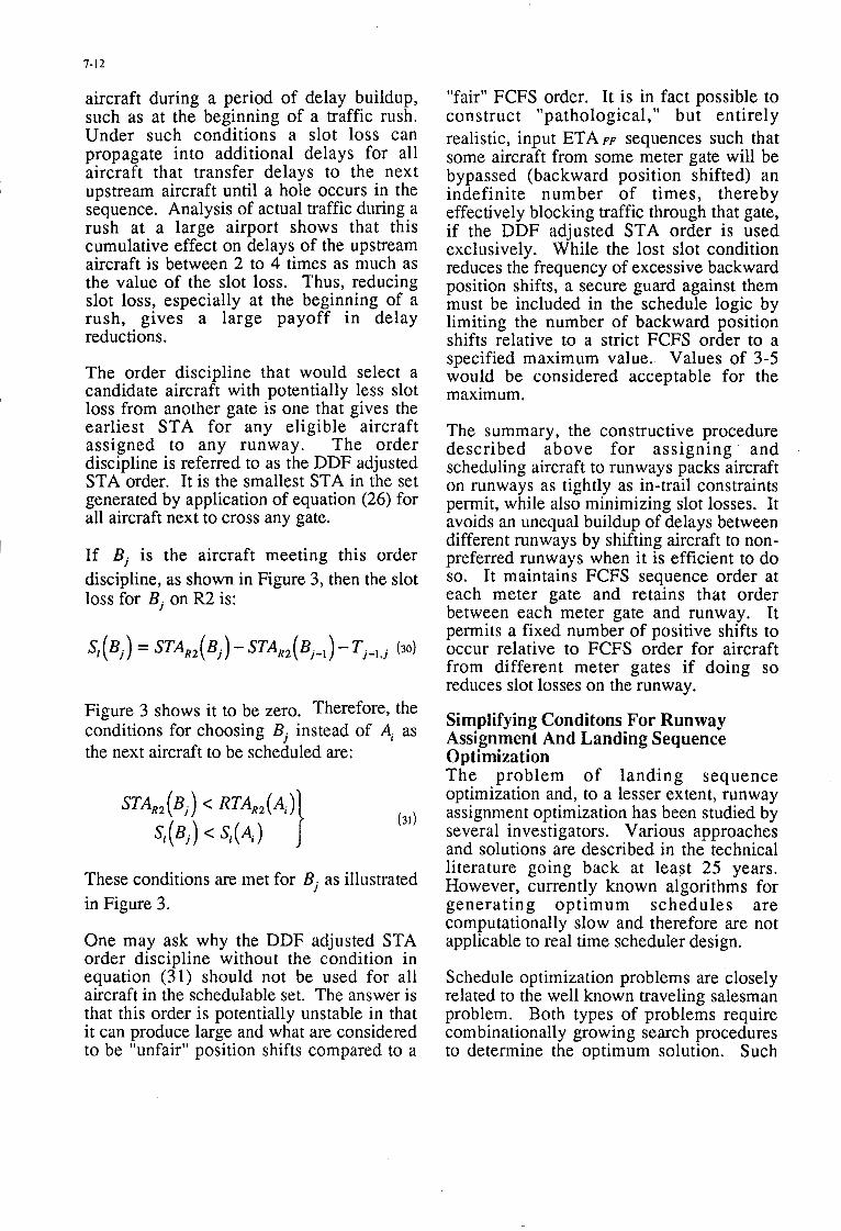
Step 1: Apply in-trail separation constraints at meter gates Let the set of scheduled times of arrival at the meter gates with in-trail constraints Ti, be {STA,,,} . Generate the STA,,'s sequentially at each meter gate starting with the earliest to arrive aircraft A1 and B1 a t gates A and B, respectively:

and similarly for gate B aircraft. For generality the Ti, parameter should be considered a function of the meter gate and stream type. This step is illustrated in Figure 2a.

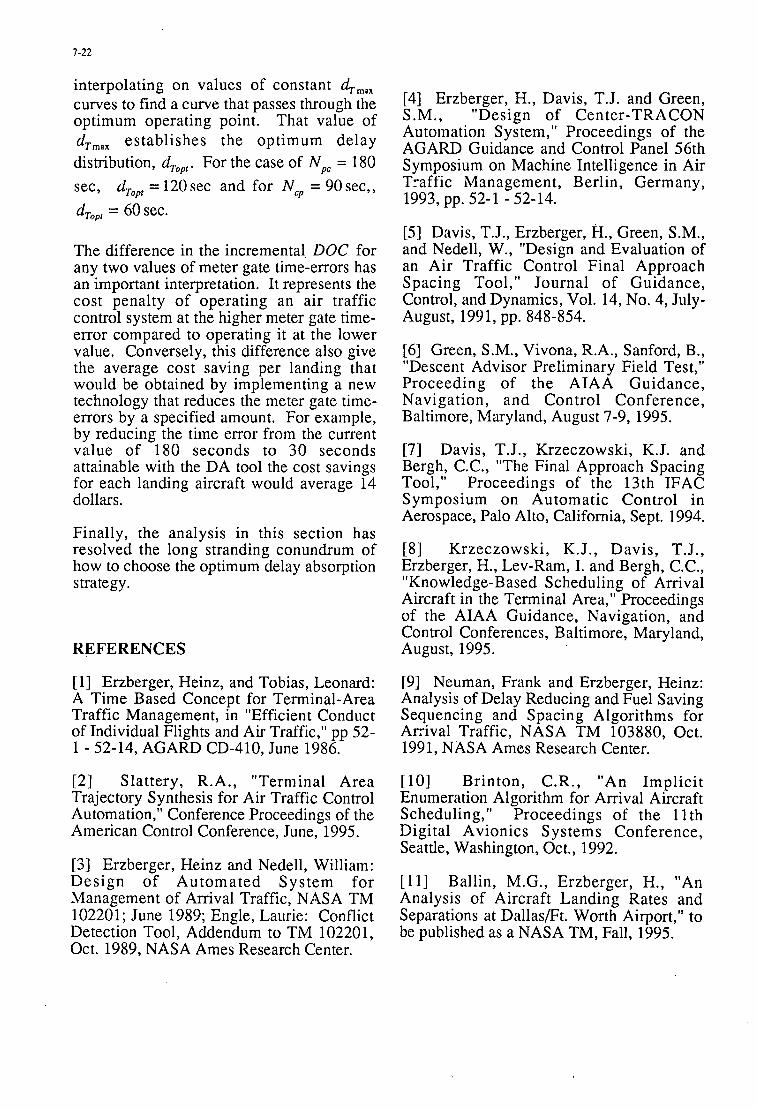
Step 2: Determining the Runway Threshold Landing Order As previously stated, the overall objective is to generate a FCFS order at the runway. However, when in-trail constraints are present at the meter gates, such as those described in step 1, the definition of FCFS at the runway becomes ambiguous. The ambiguity is removed by choosing the STAFFi,'s rather than the ETA,'s when establishing the FCFS order at the runway. Simulation and analysis have shown this choice produces both a fairer schedule overall as well as one that is slightly more efficient than a schedule that ignores the meter gate constraints.

The process begins by propagating the STAFFif's forward in time from the gates to the runway by using the TRACON transition times. If RTA(Ai) and RTA(Bj ) designate

the runway times of arrival of aircraft Ai and Bi, then:

RTA(Ai)=STA,,, (Ai)+T, (A i ) (3)

RTA( B, ) = STAFF, ( B, )+T, ( B, ) (4)

Repeating this for all schedulable aircraft results in the two sets:

( 5 )

The times in these sets represent the earliest possible landing times of the schedulable aircraft when in-trail constraints at the gates are included but in-trail constraints on final approach are ignored.

Before the FCFS landing order is determined from the sets of RTA's, an order rectifying procedure must first be performed, for the following reason. Because different aircraft types can have substantially different TRACON transition times, the RTA's in equation ( 5 ) are not necessarily in FCFS order. That is, the RTA order can become position shifted relative to the STAFFi, order for aircraft passing through the same gate. The occurrence of overtakes between aircraft in the same stream class flying from the same gate to the same runway is generally not acceptable to controllers and must be excluded by the scheduling algorithm. It is necessary to check each set of RTA's for position shifted sequences. If such sequences are found, the T, of each overtaking aircraft is increased by the smallest time increment that modifies the RTA's so as to restore them to FCFS ordered sequences. It is now assumed that the RTA's in equation (3) have already been rectified in this manner and are therefore in FCFS order.

The runway landing order list, {CP}M+N, is now obtained by merging the two sets of RTA's into a FCFS time ordered sequence list:

FCFS landing order list:

where the second indices k,Z indicate the landing order. The indices satisfy the

7-7

STA(Cl) =RTA(C,)

{ :;;{a)+ Ti, (C, , C,) STA (C,) = Greater of (7)

inequalities k k i , Z 2 j over their range of values. Figure 2b illustrates the merging and ordering process. Note that no lines connecting gate sequences and landing sequences cross, as required by the overtake exclusion.

Step (3): Computing scheduled times of arrival at the runway threshold In this step the time separations between the unconstrained runway times, the RTA's, are stretched, when necessary, to conform to the minimum time separation matrix given in Table 2. This yields the scheduled times of arrival, the STA's at the runway threshold.

The process involves inserting the appropriately chosen minimum time separation, Tit , from Table 2, between pairs of aircraft starting with the first aircraft in the known landing order, and terminating with the last. This process can be written symbolically as shown in equation set (7).

If the RTA's are closely bunched, thus requiring the Ti,'s to be inserted for a portion of the schedulable aircraft, the sequential character of equation (7) can propagate a delay ripple for successive aircraft in the landing order. The delay ripple terminates when a sufficiently large time gap occurs between successive RTA's. The delay d(C,)generated by equation (7) for the p f h aircraft in the landing order can be written as:

In addition to the scheduling constraints already described, two other types of scheduling constraints referred to as blocked intervals and reserved time slots on the runway must also be handled by the scheduling algorithm. They are specified time intervals and virtual aircraft landing times that the scheduling algorithm must avoid when generating the STA's for the list of schedulable aircraft. The logic in equation (7) can be extended in a straight forward way to handle these constraints.

The processes described in this step are illustrated by the example in Figure 2c. A blocked time interval has been included as a constraint.

Step 4: Development of Delay Distribution Function Whenever the total flow rate to a runway exceeds a certain maximum rate for a significant period of time, the separation constraints imposed by equation (7) will generate large delays. When that occurs it is said that the rate exceeds the runway capacity. Up to this point in the development of the algorithm, all delays no matter how large, would be absorbed between the meter gates and the runway. However, a group of aircraft in sequence, each with delays of several minutes to absorb in the TRACON airspace, creates excessive workload for TRACON controllers and can produce potentially

STAFF ( B, ) = STA ( B, ) - Tt = ETAFF ( B, ) (B'2 = sTAFFi, (Bz > + DDFC ( ( B2 1)

unsafe operational conditions. Center and TRACON traffic managers work diligently to control this congestion in the TRACON airspace. Analogously, the scheduling algorithm needs a mechanism for controlling congestion of TRACON airspace due to excessive delay buildup.

This step describes an analytical procedure for distributing delay between Center and TRACON airspace. The procedure involves the use of two functions referred to as Center and TRACON delay distribution functions DDF, and DDFT ,respectively, as follows:

DDF,(d ) =

D D F T ( d ) = { dT max 3 ' d'dTmax ' dT max }(IO)

where d+,.,,,is a parameter that specifies the maximum delay an aircraft is permitted to absorb in the TRACON airspace. As required, the sum of the two functions just equals the delay to be absorbed:

DDF, (d )+ DDFT (d)= d , ( 1 1 )

for all values of d . The two functions are plotted in Figure 2d. These functions are evaluated by substituting into them the delay, d , of each scheduled aircraft as computed by equation (8). Furthermore, the parameter dTmaxis itself a function that depends on the meter gate through which an

aircraft passes. The meter gate dependency allows modulation of the delay absorption parameter by the length of the nominal (undelayed) path between meter gate and runway. In general, the shorter the nominal path length (more precisely, the TRACON transition time, T , ) the less must be the maximum delay that can be absorbed along that path. In a later chapter, a method for choosing appropriate values for dTmax will be derived.

Step 5: Computing Scheduled Times of Arrival at the Meter Gates This step describes the procedures for combining the values of the Center delay distribution of step 4, the scheduled times of arrival at the runway of step 3 and the meter gate sequence order of step 2 in order to generate the STAFF' s, the scheduled times of arrival at the meter gates.

In brief, the procedure consists of a push- back of the STAFF,' s, by an amount of time calculated from the Center delay distribution. It may also be thought of as a backward propagation of delays from TRACON to Center airspace. The push-back is done sequentially for aircraft at each meter gate in such a way that the meter gate sequence order is preserved.

The procedure begins with the first aircraft in the landing order. Let that aircraft be B,, which is consistent with the example sequence in Figure 2e. Then, in accordance

7-9

with the definition in equation (6) , B,, = C,. As the first aircraft scheduled to land, it is always free of delay. The STAFF' s for all the aircraft crossing the meter gate B can then be generated sequentially as shown in equations (12), (13) and (14).

The above series of relations are also used for generating the STAFF's of aircraft crossing meter gate A. When aircraft are experiencing large delays, the second of the two quantities in the comparison test of equation (14) will be the greater of the two and thus will determine the STAFF. However, in practice, the parameters T i t a n d D D F , can assume such combinations of values that the first quantity becomes the greater of the two. By choosing the first quantity as the STAFF in that case, the logical condition "greater of" ensures that the FCFS meter gate sequence is preserved

The push-back process described here suggests an alternate method for generating a slightly different landing order and scheduled times. Instead of determining the landing order for all schedulable aircraft first, as in step 2, in the alternate method the landing order is generated during the push- back process and is therefore referred to as the push-back adjusted FCFS order method (PAFCFS).

Figure 2e illustrates the graphical construction of the schedule for the PAFCFS method . The push-back of meter gate time is shown in detail for A , .

In the PAFCFS method, the landing order of the first and second aircraft are generally unchanged.Therefore,the STA' s and STAFF' s for these two aircraft are still determined by equations (12) and (13) and their values remain unchanged. To determine the third aircraft to be scheduled to land, select the next aircraft in the FCFS sequence order at each meter gate. Following the example sequence in Figure 2, the next aircraft at gate A is A1 and at gate B i t is B3. Then compute

the in-tra aircraft:

1 meter gate times for these

Next, compute the earliest unconstrained runway times for this pair:

The next aircraft to be scheduled to land is now chosen to be the one with the earliest RTA, written symbolically as:

Next aircraft to land {A, or B3} = Arg ( lesser of

{ RTA (A, 1 9 RTA (B3 I} 1 (19)

In the example of Figure 2e, the next aircraft is A I , which represents a change in order compared to the original method. The computation of STA, DDF, and STAFFfor the aircraft so selected now parallels the previously described method. Analysis of the PAFCFS order reveals that in comparison to the original order, it tends to advance the landing order of aircraft from gates with lower flow rates relative to those from gates with higher flow rates. While this may be seen as less fair than the original method it also yields on average slightly lower delays.

After these quantities have been computed, they provide the input conditions for equations (15) - (19) to select the next aircraft to be scheduled to land. Thus in contrast to the original method, the landing order here is not known until all aircraft remaining to be scheduled are from a single gate.

EXTENSION TO MULTIPLE RUNWAYS In this chapter the basic algorithm is extended to handle the scheduling of aircraft to an airport with several landing runways. All large airports use at least two and as

7-10

many as four landing runways simultaneously under certain traffic and weather conditions. Similar to the basic algorithm, the objective here is to generate efficient initial schedules for the multiple runway case without time consuming iterative procedures. These schedules and runway assignments can then be used as the starting solution for optimizing procedures if real time computational constraints permit. The guiding principle of the runway assignment process as developed here is to assign and schedule aircraft sequentially to the runway that gives the earliest landing time while minimizing loss of full or

I fractional landing slots.

~ . . First it is necessary to generalize the definition of FCFS at the runway for the multiple runway situation. Begin by completing step 1 for the list of schedulable aircraft. Then compute the unconstrained

equations (3)-(4) of step 2 for each runway.

following development assumes two landing runways, designated as R1 and R 2 .

I runway times of arrival, the RTA's, as in

In order to avoid complex symbology, the ,

Thus, for the gate A aircraft, one can write:

and similarly for the gate B aircraft, where the RTA's and T, 's have been appended with the runway identification, R1 (or R2) . Then, for each aircraft, define the preferred runway, RP, as the one having the lesser of the T,'s:

RP(A,) = Arg { R l , R 2 }

and similarly for aircraft from all other gates. Then, the FCFS order is defined as the merged and time ordered set of the corresponding RTARp' s :

FCFS landing order list =

It would now be possible to generate scheduled landing times by inserting the appropriate minimum time separation, Ti, , between successive aircraft landing on the same runway, similar to step 3 of the single runway case. While such a schedule is feasible it may also be grossly inefficient for the following reason. At hub airports, traffic arrives in rushes from one or at most two directions, causing the one runway with the shortest transition time between the rush traffic meter gate and that runway, to become overloaded. This would occur because the FCFS order procedure defined above leaves all aircraft assigned to their preferred runways. It is, however, possible to improve upon the preferred runway assignment procedure with little additional computation, thereby providing a more efficient starting condition for subsequent runway assignment optimization steps.

The improved procedure can be used either in conjunction with the preferred runway FCFS order defined above or with the delay distribution adjusted order described in step 5. Assume to start with that the FCFS order of equation (23) is being followed. Let the next aircraft to be assigned and scheduled be Ai from Gate A, and let the next aircraft to cross gate B be B j . The preferred runways for these two aircraft are R1 and R 2 , respectively. Then it follows that:

where: Azl ( A i ) = T,, ( A i ) - T,, ( A i ) > 0 is the increment in time for Ai to transition from gate A to the non-preferred runway compared to the preferred runway. Corresponding relationships can also be written for B j . Figure 3 illustrates these concepts for an example sequence.

7-11

The next step is to calculate the S T A s for a11 combinations of aircraft next in sequence to cross any of the meter gates and all possible landing runways. Each of the STA's is calculated using the procedure described in step 3:

The four STA'sfor the example are shown at appropriate locations on the time line in Figure 3. At any step in the scheduling process, the characteristics of the relationships between values of STA and values of RTA influence the strategy for making efficient runway assignments. Two categories of characteristics can be distinguished each of which exposes particular problems in choosing the aircraft ( A, orB,) actually assigned to a runway and scheduled in this step, notwithstanding the assumed preference for FCFS order.

Standard category: Preferred runway STA' s are less than non-preferred runway STA's and/or all non-pyeferred runway S T A s are larger than the corresponding RTA' s.

The runway assignment rule for this category is straightforward. If the FCFS order defined in equation (13) in being followed, then the next aircraft to be scheduled in that order is assigned to the runway giving the earliest STA. If, instead, the pushback adjusted FCFS order is being followed, the RTA's for aircraft yet to be scheduled are updated after an aircraft has been assigned and scheduled. Then the aircraft from the gate yielding the lowest RTA for any eligible runway becomes the next aircraft to be scheduled and is assigned the runway corresponding to the earliest STA. Either scheduling order strategy provides acceptably efficient schedules and runway assignments for this category.

Potential Slot loss category: At least one STA for a non-preferred runway is equal to

the corresponding RTA and is less than the preferred runway STA. This case can be written symbolically as:

and is illustrated in Figure 3.

The potential slot loss referred to here arises from the fact that scheduling an aircraft to a non-preferred runway incurs an unavoidable delay increment of A seconds compared to scheduling i t to the preferred runway. Therefore, the quantity A establishes the maximum potential slot loss for a non- preferred runway assignment. However, the unavoidable delay increment A is not a slot loss if the delay that must be absorbed in assigning an aircraft to a non-preferred runway is larger than A for other reasons, such as meeting in-trail separation constraints with a preceding aircraft. The potential for a slot loss exists only when the earliest possible scheduled times to the two runways satisfy the conditions in equation (27). The actual slot loss, ' / ( A i ) as distinguished from the maximum potential slot loss is computed as follows:

S, ( A i ) = lesser of

A value of SI > 0 represents a fractional, or larger, landing slot opportunity that is wasted unless an aircraft from another meter gate is available and can be scheduled instead of Ai to occupy a greater portion of that slot. If such an aircraft is available, for examplel?, in Figure 3, then one of the FCFS scheduling order disciplines that had selected Ai as the next aircraft to scheduled would have to be relaxed so Bj can be scheduled instead.

The significance of slot loss derives from its cumulative effect on delays for upstream

7-12

aircraft during a period of delay buildup, such as at the beginning of a traffic rush. Under such conditions a slot loss can propagate into additional delays for all aircraft that transfer delays to the next upstream aircraft until a hole occurs in the sequence. Analysis of actual traffic during a rush at a large airport shows that this cumulative effect on delays of the upstream aircraft is between 2 to 4 times as much as the value of the slot loss. Thus, reducing slot loss, especially at the beginning of a rush, gives a large payoff in delay reductions.

The order discipline that would select a candidate aircraft with potentially less slot loss from another gate is one that gives the earliest STA for any eligible aircraft assigned to any runway. The order discipline is referred to as the DDF adjusted STA order. It is the smallest STA in the set generated by application of equation (26) for all aircraft next to cross any gate.

If Bj is the aircraft meeting this order discipline, as shown in Figure 3, then the slot loss for Bj on R2 is:

Figure 3 shows it to be zero. Therefore, the conditions for choosing Bj instead of Ai as the next aircraft to be scheduled are:

These conditions are met for Bj as illustrated in Figure 3 .

One may ask why the DDF adjusted STA order discipline without the condition in equation (31) should not be used for all aircraft in the schedulable set. The answer is that this order is potentially unstable in that it can produce large and what are considered to be "unfair" position shifts compared to a

"fair" FCFS order. It is in fact possible to con s tr u c t It p at ho 1 o g i c a1 , It b ut entire 1 y realistic, input ETA FF sequences such that some aircraft from some meter gate will be bypassed (backward position shifted) an indefinite number of times, thereby effectively blocking traffic through that gate, if the DDF adjusted STA order is used exclusively. While the lost slot condition reduces the frequency of excessive backward position shifts, a secure guard against them must be included in the schedule logic by limiting the number of backward position shifts relative to a strict FCFS order to a specified maximum value. Values of 3-5 would be considered acceptable for the maximum.

The summary, the constructive procedure described above for assigning and scheduling aircraft to runways packs aircraft on runways as tightly as in-trail constraints permit, while also minimizing slot losses. It avoids an unequal buildup of delays between different runways by shifting aircraft to non- preferred runways when it is efficient to do so. It maintains FCFS sequence order at each meter gate and retains that order between each meter gate and runway. It permits a fixed number of positive shifts to occur relative to FCFS order for aircraft from different meter gates if doing so reduces slot losses on the runway.

Simplifying Conditons For Runway Assignment And Landing Sequence 0 p t imiza t ion The problem of landing sequence optimization and, to a lesser extent, runway assignment optimization has been studied by several investigators. Various approaches and solutions are described in the technical literature going back at least 25 years. However, currently known algorithms for generating optimum schedules are computationally slow and therefore are not applicable to real time scheduler design.

Schedule optimization problems are closely related to the well known traveling salesman problem. Both types of problems require combinationally growing search procedures to determine the optimum solution. Such

7-13

procedures become computationally impractical to implement i n real time applications for all but a small number of schedulable aircraft.

To shed further light on the nature of these problems consider a FCFS ordered set of schedulable aircraft as shown in Table 3. The optimization objective of interest in scheduling is the minimization of the sum of delays of all aircraft by position shifting and runway assignment. No algorithms are known and none are thought to exist that can generate the optimum solution by operating sequentially on this time ordered set, starting with the earliest ETA aircraft. Another interpretation of the non-sequential character of the optimum solution procedure says that the choice of position shifts and runway assignments made at the beginning of the set cannot be made in isolation of, and are therefore interdependent with, such choices at the end of the set.

Now assume that the true optimum solution could be obtained for the whole set of schedulable aircraft converging on an airport by some future superfast computer. Such a solution would, however, be of little practical value in a real time air traffic control environment for two reasons. First unavoidable, unknowable and time varying errors in the computation of the ETA's upon which the optimum solution is based, render the solution non-optimum even if it is computable. Since ETA errors grow approximately proportional with the time- to-fly to the airport, the degree of non- optimality grows with increasing time-to-fly to the meter gate, or airport. Second, even if the optimum solution were known it cannot be enforced because of operational constraints inherent in the human centered air traffic control process. For a variety of reasons, sequencing and runway assignment decisions must be made when an aircraft first reaches a specified time to fly to a meter gate or runway. This time-to-fly parameter is known as the Freeze Horizon. A Freeze Horizon must be established in order to provide controllers with sufficient time and airspace to execute sequencing and runway as s i g n m en t adv i so rie s. Further m ore, controllers require the Freeze Horizon to be

held nearly constant, within one or two minutes of a nominal time.

The necessity for a stable Freeze Horizon together with the inevitability of errors in ETA's enable a crucial simplification in the formulation of the scheduling optimization problem. Instead of having to include a large number of aircraft in the combinatorial search as originally thought, thereby creating computational overload, only the few aircraft that, at any time, are within a narrow time range of the Freeze Horizon need to be considered in such a search. In practice, the number of such aircraft can be limited to two or at most three without incurring a significant loss in efficiency.

Thus, in conclusion, a careful examination of the actual operational environment for scheduling and control of arrival traffic permits a simplification of what initially appeared to be an intractable optimization problem to one that is computationally feasible for a real time scheduler.

REAL TIME SCHEDULING ALGORITHM WITH LIMITED SEQUENCE AND RUNWAY ASSIGNMENT OPTIMIZATION The previous chapter explained the need for incorporating a Freeze Horizon in the design of the real time scheduler. The need for a Freeze Horizon together with unavoidable errors in the ETA,'s conspired to permit a significant simplification in the runway assignment and sequence optimization problem. This chapter extends the basic algorithm to include both a Freeze Horizon and a limited degree of schedule optimization that is computational tractable in real time.

In addition to the Freeze Horizon, the Optimization Horizon and the Influence Horizon play crucial roles in the real time algorithm. The three horizons segregate the arrival aircraft into four sets based on the values of the ETA,'s relative to these horizons. The ETA FF time lines in Figure 4 give representative examples of these sets.

7-14

Freeze Horizon and Freeze Time-To-Fly The Freeze Horizon is defined as the sum of current time and a freeze-time-to-fly parameter, which lies in the range of 17-25 minutes. When an aircraft's estimated time- to-fly to the meter gate, as derived from its current ETA, becomes equal to or less than the freeze-time-to-fly, its runway assignment and landing sequence must be frozen at their last computed values.

0 p t imiza t ion Horizon and 0 pt imiza tion Interval The difference in time between the Optimization Horizon and the Freeze Horizon equals the Optimization Interval. Runway assignment and sequence optimization will be performed for the first P aircraft with ETA F F ' s in this interval. After runway assignments and landing sequences have been determined for these P aircraft. they will be frozen simultaneously. The Optimization Interval has a relatively narrow time range of only 2-5 minutes, reflecting; ~

the contr&ler's low tolerance for- variability in the location of the Freeze Horizon. The narrowness of the time range also ensures the maximum number of aircraft with ETA,'s in the Optimization Interval will be small, thus reducing the complexity of the optimization.

Influence Horizon and Influence Interval The Influence Interval is the difference between the Influence Horizon and the Optimization Horizon. Only aircraft with ETA,'s less than the Influence Horizon will be allowed to influence the choice of the runway assignments, and landing sequences for the P aircraft in the optimization set. Aircraft with ETA,'s later than the Influence Horizon are excluded because they are still too far away and, therefore, their ETA,'s are too uncertain to allow these aircraft to influence the runway assignment process at this time. Their influence will be felt later when these aircraft finally penetrate the Influence Horizon. Experience with the current level of ETA, accuracy suggests that the Influence Horizon should be located about 10 minutes above (later than) the Freeze Horizon.

The three horizons divide the set of ETA,'s into four subsets as illustrated in Figure 4. Aircraft below the Freeze Horizon have fixed STA F F t s and runway assignments. In this region controllers handle the aircraft so as to move the ETA,'s toward coincidence with the corresponding STA F F ' s . As aircraft approach the meter gate. Occasionally a controller may invoke commands to unfreeze and then reassign and resequence a particular aircraft or a group of aircraft in the Freeze Interval. Such commands are avoided if possible, because they generally increase workload and create complex control problems.

Three aircraft, A, Bi, andA,+l are located in the Optimization Interval in Figure 4. Runway assignment and sequence optimization is to be performed for the first P of these aircraft. This process is illustrated for P = 2 , a realistic value for a real time scheduler. It is carried out in three steps.

The first step generates the set of all runway assignments and scheduling orders for Ai , and B , producing what shall be called the comparison set. Since AiandBj pass through different meter gates, there are no sequence order constraints to be obeyed at the meter gates and therefore two scheduling orders are possible: A, Bi and Bi,Ai.

For each scheduling order all four pairs of runway assignments must be generated. For order Ai followed by Bi they are:

Ai + R1, Bi -+ R1

A, -+ R1, Bi + R2

Ai + R2, Bi -+ R2

Ai -+ R2, Bi -+ R1

These 4 pairs of runway assignments, when combined with the two possible scheduling orders, produce a total of 8 pairs of runway assignments, which constitute the comparison set.

The second step of the process generates the runway STA's for each pair in the comparison set as well as for all other aircraft below the influence horizon. In Figure 4, these other aircraft are Ai+l, Ai+2 and B j + ] . If should be noted that they inherited their runway assignments from the initialization procedure previously described, or if none is used, they are assigned to their preferred runways. Figure 4 illustrates one of the eight possible scheduling solutions that are generated in this step. Since runway assignments are fixed for each element in the comparison set, the basic algorithm can be applied to the determination of the STA's in a straight forward way.

The third and final step determines the optimum runway assignment and landing order for Ai and Bj by selecting the minimum delay schedule from among the eight trial schedules of the comparison set. The delay equivalent cost, D, of each trial schedule, k, is defined as the sum of the STA's for all aircraft below the Influence Horizon:

~ ( k ) = S T A ~ ( A ; ) + S T A ~ ( B ~ )

+ S T A ~ ( A , + ~ ) + S T A ~ ( B ~ + ] )

Where in this example, k ranges from 1 to 8. The particular value of the index k that corresponds to the minimum of the D(k) establishes the optimum runway assignment and landing order for Ai and B j . When this step is completed, the scheduling status of Ai and Bj is changed to frozen. The real time scheduler is now ready to receive a new set of updated ETA,'s and process them in a similar manner.

Estimating The Number Of Trial Schedules In The Comparison Set The number of distinct combinations of sequence orders and landing assignments for which trial schedules must be computed was shown in the preceding section to be 8 for the example of 2 landing runways and 2 aircraft in the optimization set. In order to

7-15

assess the computational load for other cases of interest, it is useful to estimate the number of such trial schedules in the comparison set. If no limit is placed on the number position shifts allowed, then the number of scheduling orders is P! for P for aircraft in the optimization set. It should be noted that the scheduling order is the same as the landing order.

Let Q be the number of landing runways. Since each aircraft in a scheduling order of P aircraft may be independently assigned to any of the Q runways, the number of possible runway assignments for each scheduling order is Q p . Therefore an estimate of what is essentially an upper limit of the number of trial schedules K, that the scheduler must compute to locate the optimum is:

K = P ! Q P (33)

Clearly, K exhibits an extremely fast growth rate even for small increments in P and Q. For example if P and Q are both increased from 2 to 3, K increases from 8 to 162, which is too large to be handled by a real time scheduler.

Limiting the position shifts to 2 reduces k to 81 for this example, but even this number of trial schedules is too large to be evaluated in real time. A current software implementation of the basic algorithm, which handles assignments to three runways, is designed for the P=l case, and thus needs to generate only three trial schedules.

A modest improvement in scheduling efficiency can be obtained, especially for the P=l case, by following the runway assignment of the freeze aircraft with a single position shift trial involving the freeze aircraft and the last- to-freeze aircraft. However the delay reduction potential of position shifting is somewhat reduced when it follows runway assignment optimization. This occurs because runway assignment optimization tends to assign aircraft with similar weight classes to the same runway, thus obviating the advantage of position

7-16

shifting for some situations. Nevertheless it still yields worthwhile benefits.

Adding A New Aircraft To The Schedule The addition to the basic algorithm that optimizes the schedules of aircraft near the freeze horizon and then transitions them from non-frozen to frozen status, the real time scheduler also contains numerous functions for handling a variety of special scheduling events. Such events can be triggered by commands from controllers or by inputs from other components of the automation system. For example, a controller may issue a command to reschedule an already frozen aircraft or reassign a group of frozen aircraft to a different runway. To handle the more complex events, for example runway configuration changes, the basic algorithm must be modified significantly. The management of these events in real time and the synthesis of algorithms to generate the proper responses increase the complexity of the final software design by an order of magnitude, (measured by lines of computer code) compared to the software design of the basic scheduling algorithm alone. Thus the software implementation of the full function scheduler based on the algorithm described in this paper contains about 45,000 lines of C code.

This section describes a modification to the basic algorithm for handling one of the most important as well frequently occurring special events; the arrival of a new aircraft. This event is signaled to the scheduler by the aircraft tracking and trajectory analysis modules of the automation system. The essential data associated with the events are comprised of the aircraft identifier, the arrival meter gate and the ETA, for the newly born aircraft. The scheduler must respond by adding this aircraft to the list of scheduled aircraft in a fair and efficient manner.

The procedure for adding the newly born aircraft is a variation of the basic algorithm. First, the aircraft is merged with the existing set of active aircraft in FCFS meter gate sequence order. This is illustrated in Figure

5 for Anm. Second, it is scheduled to the meter gate behind its lead aircraft, Ai+l in Figure 5 using the applicable meter gate in- trail constraint Ti, . Third, starting at the meter gate time STAFFi,(Anm) aircraft A , is scheduled to each of the available landing runways at the earliest time that is consistent with applicable meter gate-to-runway sequence constraints a, i n addition, is behind the last frozen aircraft. This creates the two trial STA's shown in Figure 5. Thus, on R1, A,, has to follow Ai+l with the appropriate time separation. On R2 it would have to follow Bj since the status of Bj was changed to frozen after the assignment process described in the preceding section was completed. Fourth, for each of the two trial STA's, the corresponding STA,,,, (A-) and STA,,,,(A,,) are determined I by applying the required delay distribution. Fifth, all old aircraft behind (Anm) in meter gate sequence order and below the influence horizon are rescheduled to their previously assigned runways. The rescheduling must include the appropriate delay feedback. Sixth, the runway assignment for A,, is now determined by evaluating the delay- equivalent cost function, equation (3 l), for the two trial assignments, and choosing the assignment giving the lowest cost.

In summary, during the flight history of an aircraft in Center Airspace beginning with the start of active tracking and ending at the time of meter gate crossing, the scheduler makes runway assignments for each aircraft twice. The first time is a preliminary assignment done at the start of active tracking. It ensures that every aircraft in the current schedulable list has an appropriately assigned runway. This permits the scheduler to generate what might be called pseudo schedules, so named because they are never actually controlled to, but are used only to provide continuously updated estimates of expected delays. Controllers use these estimates, displayed in graphically convenient form, to formulate control strategies. The second time the assignment

7-17

is made takes place just before the freeze and involves the optimization procedure described previously. However, it should be noted that the first assignment also influences the outcome of the optimization procedure because aircraft below the influence horizon retaining their original assignment still contribute to the value of the cost function given in equation (32).

While runway assignments are computed only twice, the STAFF'S are updated every 10-15 seconds prior to freeze. Experience with operating this scheduling algorithm in live traffic has shown that this update strategy achieves an appropriate balance between stability and responsiveness of the schedule to ETA, updates.

When an aircraft crosses a meter gate and enters TRACON airspace, i t comes under the control of TRACON automation-tools, such as the Final Approach Spacing Tool (FAST). At this time the aircraft is unfrozen and the FAST scheduler makes the final runway assignment. If the traffic is being controlled accurately to the meter gates, the final assignment will, more often than not, be the same as the previous assignment. The next chapter will examine the impact of control accuracy on the design of the scheduler in detail.

STRATEGY FOR DELAY ABSORPTION IN THE PRESENCE OF TIME CONTROL ERRORS Whenever arrival traffic demand exceeds aircraft landing capacity over a 15 minute or longer time interval a significant buildup of delay is likely to occur. After years of experience in dealing with such situations at large airports, traffic managers have learned how to anticipate the magnitude of a delay buildup and have ' devised standard procedures for absorbing the delay.

While traffic management procedures in use today generally achieve smooth traffic flow even when delays have built up significantly, controversy lingers over what is the best procedure for delay absorption. The dividing chasm in the controversy is between pilots and airline operators on the one hand

and controllers and traffic manager on the other.

Pilots and airline operators prefer delays to be absorbed close to the airport even to the point where holding is required in the TRACON airspace at low altitude. They fear that early delay absorption far from the airport does not produce sufficient traffic pressure to,achieve a high landing rate.

Traffic managers and controllers, on the other land, contend that, on balance, it is more efficient to absorb most delay in the Center airspace far from the airport so as to maintain traffic flow in the TRACON smooth and orderly. They further contend that delay absorption strategies that lead to frequent holding in the TRACON airspace create high workload for controllers and risk chaotic traffic conditions that actually reduce landing rates.

The structure of the basic scheduling algorithm described in the preceding chapters, when analyzed in combination with models of aircraft fuel consumption and accuracy of time-control at the Center- TRACON boundary can provide a rational solution to the delay absorption controversy. The solution derives from a method of analysis that determines the value of delay distribution between Center and TRACON airspace such that the average direct operating cost of delay absorption for the arrival traffic is minimized.

As indicated above, the two factors that are the key to the analysis are aircraft fuel consumption and accuracy of time control. It is well known that the minimum fuel flow rate (lbs/sec) of turbofan powered aircraft is significantly less at cruise altitude than it is at sea level altitude. Therefore, it is more fuel efficient to absorb delays at or near cruise altitude than it is at sea level. The performance manual of an aircraft contains the basic data needed to derive the relationship between fuel consumption and delay absorption at high and low altitude.

Such a relationship has been derived below for a Boeing 727 aircraft:

7-18

1 60

F = (120dc + 180dT)-

where d, is the Center delay, which is assumed to be absorbed at 30,000 ft and dT is the TRACON delay assumed to be absorbed at 3,000 ft. The quantity F is the additional fuel consumed in Ibs. due to delays d, and dT given in units of seconds. If the total delay to be absorbed is d = dc +dT , then equation (34) shows that choosing d = d, and dT = 0 minimizes the additional fuel consumption for any delay d. It therefore follows that if the total delay to be absorbed can be determined when the aircraft is still at or near cruise altitude and a method for controlling the delay exists, the most fuel efficient and, therefore, cost efficient strategy is to absorb all delay in the high altitude Center airspace and none in the low altitude TRACON airspace.

This result leads directly to the question of how the inevitable limitations in the accuracy with which delays can be absorbed in Center airspace should change the proposed delay absorption strategy.

This question is illuminated by examining the operation of the real time-scheduler. In the scheduling algorithm described in the preceding chapter, the final value of required delay absorption is determined at the time an aircraft's STAFF is frozen. This occurs at the freeze horizon when an aircraft is approximately 19 minutes of flying time from its assigned meter gate. The meter gate, located at the boundary between Center and TR.ACON airspace, therefore provides the dividing point for distributing the total delay between Center and TRACON airspace. And the delay distribution function, DDF, which is imbedded in the architecture of the basic real time algorithm, provides the mechanism for allocating the delay to each airspace on an aircraft by aircraft basis.

Thus the basic information needed to study the question posed above is to determine the expected accuracy of controlling an aircraft

to cross the meter gate at time STAFF assuming the aircraft is initially 19 minutes away from the meter gate when the control process begins.

Accuracy of control for both 19 and 30 minutes of flying time to the meter gates was recently estimated by analyzing over 3000 actual flights that landed at the DallasLFort Worth Airport. The estimates of accuracy were determined both for the metering system currently in use at the Fort Worth Center, and for the Center/TRACON Automation System which is scheduled for field tests at the Fort Worth Center. A NASA report by Mark Ballin and the author describing the accuracy analysis is in preparation [ 111. Of particular interest here are the two standard deviation errors at 19 minutes to the meter gates for the current metering system and for CTAS. They are, respectively, 180 and 90 seconds. Before developing a numerical technique for studying the effects of these errors, it is important to understand qualitatively why these errors will have an adverse effect on system performance. The adverse effect can be summarized succinctly as slot loss. It is most easily visualized when traffic is dense and all delay is being absorbed in the Center airspace. If an aircraft crosses the meter gate later that its prescribed STAFF, all aircraft scheduled behind the late aircraft at the minimum time separation will have this time error also passed on to them, similar to how a falling domino topples the next one. Since the time to fly from the meter gate to the runway is, by assumption equal to the minimum time, it is impossible to recover this slot loss completely by speeding up or short cutting the path. Moreover, similar to the runway assignment problem previously described, the total delay increment due to a fractional slot loss can be a several times the magnitude of the original time error if the error is propagated to several trailing aircraft. Thus, the putative benefits in fuel efficiency of absorbing all delays in Center airspace are being eroded by delay increments and the resulting fuel losses due to those meter gate crossing time errors. While it is true that perceptive pilots and con trollers have anecdotally referred to this

7-19

phenomenon, quantitative studies on it have not been done to the author's knowledge.

Stochastic Simulation Of Meter Gate Crossing Errors 'The effect of meter gate crossing errors was studied quantitatively by stochastic Monte Carlo simulation developed by Frank Neuman et al. and described in several NASA reports [9]. A simplified diagrammatic representation of this simulation is shown in Figure 6. The upper part of the figure represents the basic scheduling algorithm. The diagram draws attention to the two distinguishing characteristics of the algorithm, namely the delay distribution function for allocating delays and the feedback-like effect of this function through the sequential pushback of the STA, 's. The input to the algorithm is a set of ETA, 's representing the simulated traffic scenario. They are generated by a random process that has been carefully designed to match the statistical characteristics of a typical 90 minute long traffic rush at the DallasFort Worth airport. The simulation drives the algorithm with several thousand samples of such traffic rushes, all different from each other, yet statistically identical. The performance of the algorithm is measured by calculating delay and fuel consumption averages for thousands of such rush traffic samples. Although the input traffic is statistically generated , this part of the simulation produces a deterministic set of STA,'s and STA's for each randomly generated set of ETAFF 'S.

The lower part of Figure 6 represents the stochastic simulation of meter gate crossing time errors. The simulation generates an actual time of arrival, ATA,, over a meter gate for each aircraft by adding a randomly generated meter gate crossing time error,

F N,, to each aircraft's STAFF, the latter being provided by the simulation of the basic scheduling algorithm. The statistical properties of N , are chosen to match the empirically determined probability distribution of meter gate crossing errors.

Although the errors were found to be nearly normally distributed, they are approximated here by the convolution sum of three uniformly distributed random variables having the general shape shown in the figure. This approximation eliminates the somewhat unrealistic, for this problem at least, tail values found in the normal distribution. The ATAFF's now provide the input to what is referred to in the figure as the TRACON scheduler. This scheduler is identical to the basic scheduler but with dTmax set to zero. By reassigning and resequencing aircraft at the time they actually cross the meter gates, the TRACON scheduler compensates, to the degree that is possible, for the adverse effects of the meter gate crossing errors. Moreover, the twice repeated application of the sequencing and runway assignment algorithm, first at the Center freeze horizon and than at the TRACON boundary, represents the actual operation of CTAS as i t is being implemented in the field.

The output of the two parts of the simulation, where the output of the first becomes the input to the second, generates runway threshold STA 's whose values accurately reflect both the efficiencies gained by sequencing and runway assignment optimization as well as the penalties imposed by the pilot- controller errors in meter gate crossing times.

Analysis of Results The stochastic Monte Carlo simulation tool briefly described in the preceding section will now be used to investigate the quantitative re1 at i ons hip between del ay distribution strategies, meter gate time control errors and scheduling efficiency.

These relationships will be presented here for the single runway case. This case is not only important in its own right, but it also reveals the essential characteristics of these relationships more clearly than the multi- runway case. The multi-runway case, though qualitatively similar, is somewhat more complex to explain and will be covered in a NASA report.

1-20

The route structure modeled in the simulation consists of four meter gates with two independent traffic streams converging on each gate. One stream contains a mix of large and heavy jets, the other only large turboprops. The streams are independent by virtue of a required large altitude separation between them at the crossing point. Independence implies that there are no in- trail separation restrictions between aircraft in different streams converging on the same gate. The input traffic rate is 36 aircraft/hour, which is slightly above the maximum sustainable traffic level. There will thus be a significant build up of delays at this traffic level. All data points used in plotting of curves represent averages over 1000 randomly generated traffic samples, each of which contains 54 aircraft in a 90 minute rush period, or 36 aircrafthour.

The results, plotted in Figures 7-9, focus exclusively on the effects of meter gate crossing errors. The first of the figures, Figure 7, plot the delay increment Ad as a function of the TRACON delay distribution variable, dTmax , with meter gate crossing errors, N,,, as a parameter. It is seen that the origin of coordinates corresponds to Ad = 0, dTmax = 0 and Npc = 0. T h e average delay obtained for the simulated traffic scenario at these ideal operating conditions was found to be 280 seconds.

For each of the three non-zero values of N,, the delay increment Ad, decreased strongly with increasing values of dTmax. For the highest value of N,, 180 seconds, which corresponds to the crossing errors of the current operational systems, the reduction in the delay increment is especially striking, declining from 80 seconds at dTmax = O to only 1 1 seconds at dTmax = 180 seconds. This result clearly confirms the ability of TRACON delay distribution to compensate almost completely for slot loss due to meter gate time control errors. At the two lower values of N,,, the delay increments are less to start with and decline to correspondingly

lower values as dTmax is increased. The N,, = 30 seconds case establishes the practical lower limit of errors, which would be reached when the CTAS Descent Advisor (DA) becomes operational in Center airspace. The middle value of N,, = 90 seconds can be achieved with the CTAS Traffic Management Advisor. At Npc = 0, delay distribution has no effect on delay increment, as expected.

The asymptotic limits of this family of curves suggest a simple rule of thumb for choosing the optimum delay distribution. It is to choose dTmax equal to N p c . There is, however, a practical upper limit on dTmax of about 100 seconds that prevents the selection of the optimum value for N,,> 100 seconds. The upper limit reflects the limitations on the availability of airspace within the TRACON to perform complex delay maneuvers.

A significant difference in the effect of TRACON delay distribution exists between the single and multi-runway cases. In the multi-runway case, a non-zero dTmax helps to reduce delays even for N,, = 0. Analysis of this case shows that delay distribution in the TRACON mitigates the effects of meter gate in-trail constraints and potential for slot losses and, therefore, delays, when aircraft are assigned to non-preferred runways. This case will be examined in a future NASA report.

Finally, this result does support the opinion of those that believe allocating large delays to the TRACON minimizes slot losses.

A substantially different picture emerges from Figure 8, which plots the increment in fuel consumption A F as a function of the same two variables as in Figure 7. The incremental fuel consumption at dTmax = 0 and N,,=180 seconds is remarkable for its magnitude, which is 230 pounds for the average aircraft in the traffic sample. This represents a significant economic penalty in

7-2 I

fuel consumption resulting directly from time errors at the meter gates. Initially the fuel consumption strongly declines as dTmax increases. However, the distinguishing feature of the curves is that they reach a clearly defined minimum with respect to the variable dTmax. Beyond the minimizing value of dTmax the fuel consumption begins to rise again and becomes asymptotic to the N , = 0 curve. In this case, the rule of thumb for choosing the fuel optimum value of dTmax is dTrnax = 2/3 N,. This result reflects the influence of the fuel consumption trade off relation, equation (34). It shows that high values of TRACON delay distribution exact a fuel cost penalty that weighs against the benefits of incremental delay reduction shown in Figure 7.

This result gives support to the opinion of those who believe that a large amount of delay allocation in the TRACON can have adverse effects. However, the explanation for these adverse effects given here differs in essential ways from the anecdotal arguments that have heretofore been advanced against large TRACON delay distributions.

Introduction To A Unification Principle Of Delay Distribution The conundrum of delay distribution exposed in the preceding section has a rational resolution originating in the definition of direct operating cost, a widely used measure in the economics of airline operations. Direct operating cost, DOC, is commonly defined as the sum of the cost of time and the cost of fuel as follows:

(35) DOC= TCT + FCF

where T is the time to fly a trajectory in seconds, F is the fuel consumption of a trajectory in lbs. and CT and C, are cost factors for converting time and fuel to DOC measured in dollars. Airline operations analysts can provide data for deriving the values of cost factors CTandCF, applicable to the average aircraft in an airline's fleet.

Such data were obtained from a large US airline whose aircraft fleet can be approximated by a Boeing 727. From this data the following relationship was derived:

(36) F = lODOC-2T

The choice of F as the dependent variable anticipates the use of equation (36) in the analysis to follow.

To prepare for the application of equation (36), Figures 7 and 8 have been combined in a two parameter family of curves sometimes referred to as a carpet plot. In this carpet plot, Figure 9, fuel and time increments may both be considered dependent variables plotted along vertical and horizontal axes, respectively. The independent variables are the parameters dTmax and N,.

The unification principle may now be defined as the process by which the carpet plot of fuel and time increments is combined with the time-fuel-DOC relationship given by equation (36) to select the delay distribution strategy that minimizes the increment in direct operating cost for the average aircraft during the rush traffic period. Note that since equation (36) is linear in all variables, incremental variables can directly replace the original variables in equation (36) without changing its form.

The process can be understood by super imposing the DOC increment curves derived from equation (36) on the time-fuel coordinates of Figure 9. Then it can be shown that the unification principle is satisfied at the point of tangency of a linear DOC curve with a specific N,, curve. The value of DOC that produces tangency to the curve of a selected value of N , gives the lowest possible DOC increment corresponding to that value of N,. It therefore defines the optimum operating point for the selected value of N,. The final step is to select the delay distribution parameter, d,,,, , corresponding to the optimum operating point. That is done by

7-22

interpolating on values of constant dTmax curves to find a curve that passes through the optimum operating point. That value of dTmax establishes the optimum delay distribution, dTopr. For the case of N,, = 180 sec, dTopt = 120sec and for Ncp = 90sec,, dTopt = 60 sec.

The difference in the incremental DOC for any two values of meter gate time-errors has an important interpretation. It represents the cost penalty of operating an air traffic control system at the higher meter gate time- error compared to operating it at the lower value. Conversely, this difference also give the average cost saving per landing that would be obtained by implementing a new technology that reduces the meter gate time- errors by a specified amount. For example, by reducing the time error from the current value of 180 seconds to 30 seconds attainable with the DA tool the cost savings for each landing aircraft would average 14 dollars.

Finally, the analysis in this section has resolved the long stranding conundrum of how to choose the optimum delay absorption strategy.

REFERENCES

[ 13 Erzberger, Heinz, and Tobias, Leonard: A Time Based Concept for Terminal-Area Traffic Management, in "Efficient Conduct of Individual Flights and Air Traffic," pp 52- 1 - 52-14, AGARD CD-410, June 1986.

[2] Slattery, R.A., "Terminal Area Trajectory Synthesis for Air Traffic Control Automation," Conference Proceedings of the American Control Conference, June, 1995.

[3] Erzberger, Heinz and Nedell, William: Design of Automated System for Management of Arrival Traffic, NASA TM 102201; June 1989; Engle, Laurie: Conflict Detection Tool, Addendum to TM 102201, Oct. 1989, NASA Ames Research Center.

[4] Erzberger, H., Davis, T.J. and Green, S.M., "Design of Center-TRACON Automation System," Proceedings of the AGARD Guidance and Control Panel 56th Symposium on Machine Intelligence in Air Traffic Management, Berlin, Germany, 1993, pp. 52-1 - 52-14.

[5] Davis, T.J., Erzberger, H., Green, S.M., and Nedell, W., "Design and Evaluation of an Air Traffic Control Final Approach Spacing Tool," Journal of Guidance, Control, and Dynamics, Vol. 14, No. 4, July- August, 1991, pp. 848-854.

[6] Green, S.M., Vivona, R.A., Sanford, B., "Descent Advisor Preliminary Field Test," Proceeding of the AIAA Guidance, Navigation, and Control Conference, Baltimore, Maryland, August 7-9, 1995.

[7] Davis, T.J., Krzeczowski, K.J. and Bergh, C.C., "The Final Approach Spacing Tool," Proceedings of the 13th IFAC Symposium on Automatic Control in Aerospace, Palo Alto, California, Sept. 1994.

[8] Krzeczowski, K.J., Davis, T.J., Erzberger, H., Lev-Ram, I. and Bergh, C.C., "Knowledge-Based Scheduling of Arrival Aircraft in the Terminal Area," Proceedings of the AIAA Guidance, Navigation, and Control Conferences, Baltimore, Maryland, August, 1995.

[9] Neuman, Frank and Erzberger, Heinz: Analysis of Delay Reducing and Fuel Saving Sequencing and Spacing Algorithms for Arrival Traffic, NASA TM 103880, Oct. 1991, NASA Ames Research Center.

[ l o ] Brinton, C.R., "An Implicit Enumeration Algorithm for Arrival Aircraft Scheduling," Proceedings of the 11 th Digital Avionics Systems Conference, Seattle, Washington, Oct., 1992.

[ l l ] Ballin, M.G., Erzberger, H., "An Analysis of Aircraft Landing Rates and Separations at DallasEt. Worth Airport," to be published as a NASA TM, Fall, 1995.

7-23

Figure 1 - Airspace Structure and Arrival Routes

7-24

STAFFit ETA FF RTA

STAFFit ETA

FF Gate A Gate A Runway Gate B Gate B

A 2 I

A 1 - Figure 2. Basic Scheduling Algorithm:

(a) Adding in-trail constraints at the meter gates

STAFFit ETA FF

A A

RTA

Runway Gate B Gate 6 ETA FF STAFFit Gate A Gate A

/ \ Blocked Landing Order: Slot

Figure 2 b. Determining Landing Order

7-25

FF FFit STAFFit ETA FF STA ETA

Gate A Ga

A 2 - A1 -

! A Runway

A Gate B

A Ga

A 2 7r

Figure 2 c. Determining the Runway STAs

delay

Tmax d delay in Center: DDFC /

1

delay in TRACON: DDF,

total delay to be absorbed: d

Figure 2d - Delay distribution function

1-26

ETA FF FFit FFit ETA FF STA

Gate A

A 2 - A1 - -

Gal 1

A Runway Gate B Gate B

A 2

Blocked Slot

/ I 0

0 0

0

I 5

1 T Note: DDF Pushback Adjusted

Order Chooses A before B 3

I I &

Tit - -RTA (B3) \

~

Figure 2 e. Pushback of STA FF's using DDF

7-21

Time I I I I I I t I I

- - -m- I I !

I I I I I

I I I

1--- - - -

I I

I I I I I I

R1 R2

Gate A Aircraft -

I I I I I I I I I I I I I

I - - 1-- I I ::--:/:: I

t 4 - 1 - I I ' I @-- I I

I I I I A21(B j ) I I

?-1- - - - -

I I I I

I TJisJ . - + - - - - - - - _ I

I I I I I I I I

R2 4 Gate B Aircraft

Figure 3 . Choosing a non-FCFS order and runway assignment that minimizes slot loss

7-28

STA STA STA ETA FF FF FF R2 FF R 1

STA ETA

Gate A Gate B Gate B Gate A

T t Time

c

/ /

, ifluence- - - Horizon

Ai+2 / /

lptimization . . .

t t I

Horizon - - - Freeze l/ I

I I

i Influence Horizon =\

Optimiza tior Horizon

Freeze Horizon

Unfilled boxes and dashed lines indicate one of the eight possible trial schedules generated in finding the optimum runway assignments for 4 and E5 .

Figure 4 . Illustration of real time scheduling algorithm

1-29

ETA STA STA STA STA ETA FF FF R1 R2 FF FF

Gate A Gate A Gate B Gate B

Unfilled boxes show the two trial schedules for A,, and affected aircraft below the influence horizon thae must be rescheduled

on R1 and R2

Figure 5. Illustration of real time scheduling algorithm: Adding a new aircraft to the scheduled list

7-30

ETAff's of input

Sequential STAff Pushback

.Runway Allocation .Sequence Optimization

OUTOUT: *Time Over Threshold (STA's .Total Delay: d

Delay Distribution Function

Meter Gate Crossing Times:

total delay to be absorbed, d I

TRACON Scheduler

Reallocate to Runways Resequence to Threshold

STA's

r - - m s 1 1 1 1 1 1 * * * * * IA Figure 6.- Stochastic Monte Carlo Simulation of Scheduler I 4 N p c + I

80

60

40

20

Y

Figure 7.- Average delay increment for 36 aircrawhour for a single runway vs dTmm

7-3 I

.............. ............ ............. .............. ............. ........... ............ I i 1

.? j ! _j.__ ! __: I i i ......... .. t ._ ............ . 1 t t t +

0 100 200 dTmax [sec]

Figure 8.- Incremental fuel vs dTmax

Average incremental delay [sec] Figure 9.- Carpet plot