Atmos. Chem. Phys., 14, 10619–10630, 2014www.atmos-chem-phys.net/14/10619/2014/doi:10.5194/acp-14-10619-2014© Author(s) 2014. CC Attribution 3.0 License.

Air quality in Delhi during the Commonwealth Games

P. Marrapu 1,2, Y. Cheng2,3, G. Beig4, S. Sahu5, R. Srinivas4, and G. R. Carmichael1,2

1Department of Chemical and Biochemical Engineering, University of Iowa, Iowa city, USA2Center for Global and Regional Environmental Research, University of Iowa, Iowa city, USA3Multiphase Chemistry Department, Max Planck Institute Chemistry, Hahn-Meitner-Weg 1, Mainz, Germany4Indian Institute of Tropical Meteorology (Ministry of Earth Sciences, Govt. of India) Dr. Homi Bhabha Road,Pashan, Pune, India5Forschungszentrum Julich Gmbh, IEk-8:Troposphere, 52425 Julich, Germany

Correspondence to:P. Marrapu (pallavi-marrapu@uiowa.edu)

Received: 3 August 2013 – Published in Atmos. Chem. Phys. Discuss.: 17 April 2014Revised: 16 August 2014 – Accepted: 1 September 2014 – Published: 9 October 2014

Abstract. Air quality during the Commonwealth Games(CWG, held in Delhi in October 2010) is analyzed using anew air quality forecasting system established for the games.The CWG stimulated enhanced efforts to monitor and modelair quality in the region. The air quality of Delhi during theCWG had high levels of particles with mean values of PM2.5and PM10 at the venues of 111 and 238 µg m−3, respectively.Black carbon (BC) accounted for∼ 10 % of the PM2.5 mass.It is shown that BC, PM2.5 and PM10 concentrations arewell predicted, but with positive biases of∼ 25 %. The di-urnal variations are also well captured, with both the obser-vations and the modeled values showing nighttime maximaand daytime minima. A new emissions inventory, developedas part of this air quality forecasting initiative, is evaluated bycomparing the observed and predicted species-species corre-lations (i.e., BC : CO; BC : PM2.5; PM2.5 : PM10). Assumingthat the observations at these sites are representative and thatall the model errors are associated with the emissions, thenthe modeled concentrations and slopes can be made consis-tent by scaling the emissions by 0.6 for NOx, 2 for CO, and0.7 for BC, PM2.5, and PM10. The emission estimates for par-ticles are remarkably good considering the uncertainty in theestimates due to the diverse spread of activities and technolo-gies that take place in Delhi and the rapid rates of change.

The contribution of various emission sectors includingtransportation, power, domestic and industry to surface con-centrations are also estimated. Transport, domestic and in-dustrial sectors all make significant contributions to PM lev-els in Delhi, and the sectoral contributions vary spatiallywithin the city. Ozone levels in Delhi are elevated, with

hourly values sometimes exceeding 100 ppb. The continuedgrowth of the transport sector is expected to make ozonepollution a more pressing air pollution problem in Delhi.The sector analysis provides useful inputs into the design ofstrategies to reduce air pollution levels in Delhi. The con-tribution for sources outside of Delhi on Delhi air qualityrange from∼ 25 % for BC and PM to∼ 60 % for day timeozone. The significant contributions from non-Delhi sourcesindicates that in Delhi (as has been show elsewhere) thesestrategies will also need a more regional perspective.

1 Introduction

Rapid industrialization and urbanization over the past fewdecades have led to high levels of outdoor air pollutionthroughout the world. This is particularly true in the megaci-ties of Asia, where high concentrations of aerosols and othercriteria pollutants have large impacts on the health and wel-fare of its citizens (Guttikunda et al., 2005). Small ambientparticles can penetrate deeply into sensitive parts of the lungsand can cause or worsen respiratory disease, such as emphy-sema and bronchitis, and can aggravate existing heart dis-ease, leading to increased hospital admissions and prema-ture death (Drimal et al., 2010). These particles and othershort-lived radiative forcing agents such as ozone also absorband scatter solar radiation and impact weather and climate.The warming effect of all the greenhouse gases together isestimated at 2.5 watt m−2, while the net cooling effect ofaerosols is 0.7 watt m−2 according to the Intergovernmental

Published by Copernicus Publications on behalf of the European Geosciences Union.

10620 P. Marrapu et al.: Air quality in Delhi during the Commonwealth Games

Figure 1. Nested model domains used in the Commonwealth Games forecasts and analysis. Insert shows the locations of the observationssites.

Panel of Climate Change (IPCC, 2007). The high levels ofblack carbon (BC) in Asia are of particular interest, becauseof its dual role in impacting human health and in acting likea greenhouse gas, absorbing solar radiation causing warm-ing of the atmosphere. Ramanathan and Carmichael estimatethat BC is the second most important warming agent (behindCO2) (Ramanathan and Carmichael, 2008). For these rea-sons there is currently mounting interest in developing strate-gies that will both reduce the levels of air pollutants and re-duce global warming. These strategies often develop first inmegacities, where air quality and energy policies respond tothe rapid needs associated with the widespread urbanization.Effective management of air quality requires enhanced un-derstanding of the sources of pollution and their effects onhuman health and climate.

In this paper we analyze BC and other pollutants in Delhi(28◦35′ N, 77◦12′ E, 217 m mean sea level (m.s.l.)), the cap-ital city of India and the largest city by area and the sec-ond largest by population in India. It is the eighth largestmegacity in the world with more than 18 million inhabi-tants. Delhi hosted the Commonwealth Games (CWG), amulti sport event involving 73 countries, in October 2010.This high profile event provided an opportunity to acceler-ate efforts to improve air quality. To support the CWG air

pollution monitoring was enhanced, a new emissions inven-tory was developed (Sahu et al., 2011) and new air qualityforecasting efforts were initiated. In this paper we use theWeather Research Forecast- Chemistry (WRF-Chem model,Grell et al., 2005) to simulate the air quality during the CWGand evaluate its performance by comparing the predicted me-teorology and concentrations of BC and other criteria pollu-tants with observations. We present spatial patterns of BC,PM2.5 and PM10, CO, NOx, and O3 over Delhi and estimatethe contributions from specific source sectors (transportation,power, industrial, and domestic). Such sector information isneeded to help guide the development of effective pollutionreduction measures. We also evaluate the emission estimatesby analyzing observed and predicted species ratios.

2 Approach

2.1 WRF-Chem configuration and domain

The CWG air quality forecast system is based on the WRF-Chem model. Four nested domains were used in the analy-sis and they are shown in Fig. 1. The outer domain coveredSouth Asia from 50 to 120◦ E and 0 to 55◦ N at a horizon-tal resolution of 45 km, with 131× 131 grid cells. The next

Atmos. Chem. Phys., 14, 10619–10630, 2014 www.atmos-chem-phys.net/14/10619/2014/

P. Marrapu et al.: Air quality in Delhi during the Commonwealth Games 10621

Table 1. Important input settings of the WRF-Chem model used in this study.

Feature Option Description

Chemical Mechanism CBMZ Carbon Bond Mechanism v.Z with MOSAIC 4aerosol bins (Zaveri, R. A. et al., 2008)

Microphysics Lin scheme Sophisticated scheme with ice,snow, and graupel processes.

Long-wave Radiation Rapid Radiative Transfer Model (RRTM) Accounts for multiple bands,trace gases, and microphysics

Shortwave Radiation Goddard shortwave Two-stream multi-band scheme with ozonefrom climatology and cloud effects.

Surface Layer MM5 similarity Based on Monin–Obukhov with Carlson–Bolandviscous sublayer and standard similarityfunctions from look-up tables.

Anthropogenic Emissions Delhi Inventory & INTEX-B Delhi inventory at 1.67 km resolution IntercontinentalChemical Transport Experiment B (INTEX-B) data at0.5◦ × 0.5◦ resolution (Zhang et al., 2009).

Biogenic Emissions MEGAN MEGAN Model of Emissions of Gases and Aerosols from Nature,biogenic emissions online based upon the weather, land use data.

Boundary Conditions MACC Monitoring Atmospheric Composition & Climate,a global 3-D chemical transport model driven byoffline meteorological fields.

Table 2.Anthropogenic emissions and % sectoral contribution for Delhi.

Contribution From each Anthropogenic Sector

Species Tonnes/Day Transportation Power Industry Domestic

SO2 81 12.9 % 48.7 % 25.2 % 13.2 %NOx 598.5 69.4 % 13.2 % 4.5 % 12.9 %CO 1320.3 43.7 % 0.2 % 4.0 % 52.0 %PM10 344.8 86.8 % 7.9 % 4.6 % 0.8 %PM2.5 128.6 52.6 % 9.9 % 15.3 % 22.2 %BC 36.9 58.9 % 3.0 % 6.6 % 31.5 %OC 35.1 30.5 % 5.6 % 10.6 % 53.3 %NMOC 852.4 58.4 % 1.2 % 5.2 % 35.3 %

domain focused on the northern regions of India covering theIndo Gangetic plain at a resolution of 15 km with 127× 127grid cells. The two inner domains covered the Delhi region atresolutions of 5 km with 55× 55 grid cells and 1.67 km with75× 75 grid cells. For all domains 27 vertical levels wereused with a maximum height of∼ 20 km. The model config-uration is summarized in Table 1. This configuration enablesdirect, indirect and semi direct aerosol radiative feedbacks tobe included in the analysis. The Carbon Bond Mechanismversion Z (CBMZ) with the MOSAIC aerosol module using4 size bins was employed.

2.2 Emissions

A new detailed emissions inventory was prepared by IndianInstitute of Tropical Meteorology (IITM) Pune, Maharastrafor the Delhi area at a resolution of 1.67 km2. The emis-

sion inventory covered the National Capital Region Delhi(NCR) (∼ 70 km× 65 km) and the surrounding areas (in to-tal covering 115.23 km× 138.6 km). The emission data wasdeveloped for NOx, CO, BC, PM2.5, PM10, OC, VOC andSO2 for four sectors (i.e., power, industrial, transport, resi-dential). This NCR area was extensively studied through afield campaign made during March–May 2010, which col-lected relevant primary and secondary data with high resolu-tion. This data included vehicular along with the type of fuelused, point source locations for manufacturing industries lo-cated within Delhi, and biofuel usage from slums, hotels andstreet vendors (Sahu et al., 2011). For the rest of the areabeyond the NCR region emissions were based on proxies asnew primary data were not generated in this region.

The emission totals by species and sector for Delhi aresummarized in Table 2. The transport sector accounts for the

www.atmos-chem-phys.net/14/10619/2014/ Atmos. Chem. Phys., 14, 10619–10630, 2014

10622 P. Marrapu et al.: Air quality in Delhi during the Commonwealth Games

more than 40 % of the emissions for all species with the ex-ception of SO2 and OC. Delhi is a densely populated city andhas approximately 4 million on road vehicles and the num-ber increases at a rate of∼ 10 percent per year (Mohan et al.,2006). The PM2.5 and PM10 transport sector emissions in-clude windblown road and construction dust sources, whichcomprise∼ 50 % of the total transportation sector emissions.For SO2 power generation and industrial sources are the mostimportant sectors. The domestic sector is large for CO, OC,BC and NMOC (non-methane organic compounds).

The spatial distribution of emissions was based on road-ways, and locations of power plants, slums and major in-dustries using various Delhi data sets (Sahu et al., 2011).The emissions were transferred into the WRF-Chem model-ing system using the Emission Preprocessor Model (EPRES)designed by Dr. M. Lin (Center for Sustainability and theGlobal Environment at University of Wisconsin-Madison)and modified by Dr. Y. F. Cheng (Center for Global and Re-gional Environmental Research at the University of Iowa).EPRES does two things, first it speciates the total VOC emis-sions based on the chemical mechanism (i.e., Carbon BondMechanism version Z, CBM-Z), and second it horizontallyinterpolates the emission inventory onto the model grids.When interpolating the emissions, EPRES reads in the ini-tial grid of the inventory from the WPS/WRF (Weather Pre-processing System) output and then utilizes the Input/OutputApplications Programming Interface (I/O API) mass conser-vative interpolation subroutine to interpolate the emissionsonto the WRF model grids. All the interpolated species wereconverted into WRF-Chem required units. After wards, themapped emissions were distributed into vertical layers, i.e.,70 % was distributed at the surface and 30 % was uniformlydistributed to the grids up to∼ 1000 m (grids 2–6 in thisapplication). Diurnal profiles were also applied. The diur-nal variability of BC emissions is shown in Fig. 7, and ex-hibits two peaks, one in early morning and the second in earlyevening associated with traffic and cooking activities.

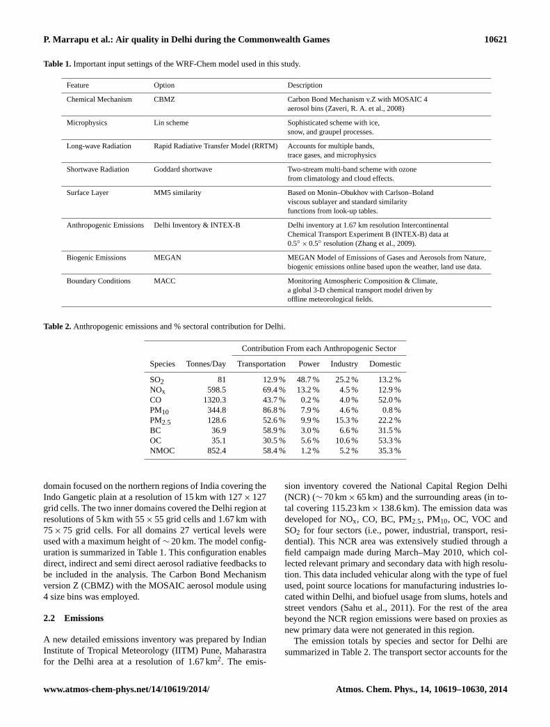
Figure 2 shows the emission distributions of NOx andPM2.5 over Delhi. The emissions of all the primary speciesfor the inner grid are shown in the Supplemental Fig. S1. Thespatial distribution reflects the various activities within andaround the city. The NOx and PM2.5 emissions show intenseemissions within the city and along roadways, with spatialdifferences reflecting different contributions by sector. Ge-ographically Delhi is surrounded by industrially developedcities such as Gurgoan and Noida. Construction is activewithin and around the city and as a result many cement indus-tries and brick kilns are situated in and around Delhi, addingto the increasing particulate emissions associated with roadand construction dust. Extensive usage of wood and charcoalstoves for cooking is prevalent in the slums and in the outskirts of Delhi and high BC emissions (∼ 30 % of total) oc-cur in association with these activities (Sahu et al., 2008).The sectoral distributions of the BC emissions are shown inFig. 3. These show clearly the locations of the power plants,

Figure 2. Emission distributions of NOx (top) and, PM2.5 inTonnes yr−1 over Delhi.

industrial clusters, the distribution of slums and the majortransportation networks. The venues for the CWG were clus-tered in the eastern half of Delhi city denoted by the com-pleted outline in the center of the domain (see Fig. 4). Theseare regions most heavily impacted by domestic and industrialsources.

The INTEX-B (Intercontinental Chemical Transport Ex-periment) emissions (Zhang et al., 2009) were used overthe outer three domains. Biogenic emissions were calculatedhourly online using MEGAN (Emmons et al., 2010). Thedust emissions were turned off during the run time of themodel, since the post monsoon period is a period with in-significant wind-blown soil dust impacts on Delhi. No agri-cultural fire emissions were included, reflecting that in thispost monsoon period no harvesting takes place.

Atmos. Chem. Phys., 14, 10619–10630, 2014 www.atmos-chem-phys.net/14/10619/2014/

P. Marrapu et al.: Air quality in Delhi during the Commonwealth Games 10623

Figure 3. Sector contributions to Black Carbon emissions (%) for Delhi.

Figure 4. Locations of the monitoring stations for the Common-wealth Games.

2.3 Boundary conditions and simulation procedure

To consider the influence of sources outside of the largestdomain, boundary conditions from the European Centrefor Medium-Range Weather Forecasts (ECMWF) MACC(Monitoring Atmospheric Composition and Climate) projectthat operates a data-assimilation and modeling system fora range of atmospheric constituents that are important forclimate, air quality and surface solar radiation (http://www.gmes-atmosphere.eu/) were used. The meteorology was ini-tialized using National Oceanic and Atmospheric Admistra-tion (NOAA) FNL Operational Global Analysis data usingthe WPS subprogram and simulations were done in 5-dayperiods each with two days of spin up time.

2.4 Observations

A total of 10 new automatic air pollution and meteorologymonitoring stations were installed for the CommonwealthGames and were placed at different venues across the city(i.e., Commonwealth Games Village (CWG), IITM Delhi(IITM), Yamuna Sports Complex (YSC), Indira GandhiSports Complex (ISC), M.Dhyan Chand National Stadium(MDS), Jawaharlal Nehru Sports Complex (JSC), Thyagaraj

www.atmos-chem-phys.net/14/10619/2014/ Atmos. Chem. Phys., 14, 10619–10630, 2014

10624 P. Marrapu et al.: Air quality in Delhi during the Commonwealth Games

Figure 5. Spatial distributions of calculated 20-day mean concentrations of surface BC (µg m−3) and daytime (9.30am–6.30pm IST) ozone(ppb) over Delhi. For ozone daytime means are shown.

Sports Complex (TSC), University of Delhi (UD), IGI-Airport (IGI) and finally Talkotaroe Garden (TG)) as shownin Fig. 4. BC, CO, NO, NO2, O3, and PM2.5 and PM10were measured at hourly intervals over the span of 2 weeksfrom 26 September 2010 to 15 October 2010. Similar tothe air quality species, meteorology parameters (i.e., windspeed (m s−1), wind direction (deg), temperature (◦C), andrelative humidity (%)) were also measured. Ozone was mea-sured with a photometric UV analyzer (Thermo-49i) and NOand NO2 with chemiluminescence analyzer (Thermo-41i).BC was measured with the Magee Scientific aethalometer(Model AE31) and, PM2.5 and PM10 using BETA attenua-tion analyzers (Beta Met One BAM 120).

3 Results and discussions

The WRF-Chem model was run for the period 26September–16 October 2010. The analysis in this paper fo-cuses exclusively on the Delhi region (the innermost grid).

3.1 Meteorology

The Commonwealth Games were held during the post mon-soon season, a transition between the summer monsoon andwinter. The general situation in India is that in mid Septem-ber the monsoon shifts from the southwest monsoon to thenortheast monsoon. This brings in air masses from the north-ern parts of the country (Ghude et al., 2008). During theCWG the surface winds were most frequently from the NNWand low (< 3 m s−1). Winds from the ESE were less frequentbut of higher speeds.

The predicted meteorology was compared with surface ob-servations at two monitoring stations (results are typical ofother sites). The statics of the comparison are shown in Ta-ble 3. The model has a dry bias (under predicts RH), slightlyunder predicts peak day time temperatures by 1–2◦ (∼ 5 %),and is biased high in wind speed. The model captures the low

Table 3. Comparison of predicted meteorological parameters withobservations at the surface monitoring sites.

Temp (◦C) Wind speed RH (%)(m s−1)

Mean-Obs 29.0 1.3 53.5Mean-Model 28.7 2.2 45.8Bias Error 7.7 1.3 7.0RMSE 13.6 2.9 33.9R 0.9 0.5 0.7

wind speeds, but the observations often are less than 1 m s−1,which the model estimates at 1–3 m s−1.

3.2 Air pollutants in Delhi

3.2.1 Aerosols

The predicted period mean surface concentrations of BC areshown in Fig. 5 (PM2.5, PM10 and CO show a very sim-ilar spatial distribution). Black carbon concentrations ex-ceed 25 µg m−3 in the center of the domain where emis-sions from the residential and industrial sectors are both high(see Fig. 3). PM2.5 and PM10 levels are very high in thisarea with period mean values of 220–350 µg m−3 and 350–550 µg m−3, respectively, values which greatly exceed theNational Ambient Air Quality standards of 60 µg m−3 and100 µg m−3, respectively.

The hourly surface concentrations from all the observa-tion stations over the entire time period were combined andtheir distributions are presented in Fig. 6. The variability be-tween the stations is shown by the bars that reflect the valuesat the stations that had the highest and lowest values. Themean value for BC from all the sites is 9.5 µg m−3, with min-imum and maximum site values of 4.4 and 13.1 µg m−3. Theoverall mean values for PM2.5 and PM10 (along with maxi-mum and minimum site means) are as follows: 111 µg m−3

Atmos. Chem. Phys., 14, 10619–10630, 2014 www.atmos-chem-phys.net/14/10619/2014/

P. Marrapu et al.: Air quality in Delhi during the Commonwealth Games 10625

Figure 6. Comparison of the distributions of observed and modeledhourly concentrations using data from all sites. Base corresponds tofull emissions whereas control shows results where the NOx emis-sions were reduced by a factor of 3.

Figure 7. Mean diurnal variation in boundary layer height, emis-sions and BC concentrations from model and observations at theDhyan Chand Stadium site.

(77–144 µg m3) and 238 µg m−3 (200–306 µg m−3), respec-tively. The distributions of the calculated values are alsoshown in Fig. 6. In general the predicted values show a simi-lar distribution, but with a positive bias (∼ 30 %).

Further insights into the pollutant distributions in Delhiare found by analyzing the diurnal variations. The 20-dayaverage diurnal cycle of BC observed at Dhyan Chand Sta-

Figure 8. Percent contribution of each species to total PM2.5 atDhyan Chand Stadium.

dium is shown in Fig. 7, along with the diurnal emissionsused in the model and the predicted planetary boundary layer(PBL) height. The BC observations show a strong diurnal cy-cle, with minimum in the mid-afternoon when the PBL is thehighest and maximum in late evening when the PBL height isat a minimum and emissions are at their highest. The eveningand early morning features reflect the cooking and traffic pat-terns and the trapping of these surface emissions by the shal-low night time mixing layer. These diurnal features are wellcaptured by the model, which suggests that the diurnal pat-tern used in the emissions accurately reflect these activities.The daytime values are accurately captured, while the nighttime values are biased high. This suggests that the daytimePBL is reasonably well predicted, but the nighttime valuesmay be too low. The diurnal profiles of PM2.5 and PM10 ex-hibit similar diurnal variations as BC, with minima duringmid-afternoon and peak values at night, but with less asym-metry between mid-night and 6 a.m. IST values, reflectingtheir stronger dependency on traffic patterns.

The predicted mean composition of PM2.5 at DhyanChand stadium is shown in Fig. 8. (There is only very slightvariability in the percent contribution at the different moni-toring stations.) BC accounts for about 8 % of the fine modemass and is greater than that for sulfate. OC accounts for∼ 30 % and other primary PM (from unpaved roads, con-struction etc.) accounts for the largest fraction. Nitrate con-tribution exceeds that of sulfate.

3.2.2 Gaseous pollutants

The hourly surface observations of CO, NO, NO2, NOx andO3 are also shown in Fig. 6. The mean observed CO is1.7 ppm, with station minimum and maximum of 1.1 and2.8 ppm. The mean NOx value is 68 ppb, with minimum and

www.atmos-chem-phys.net/14/10619/2014/ Atmos. Chem. Phys., 14, 10619–10630, 2014

10626 P. Marrapu et al.: Air quality in Delhi during the Commonwealth Games

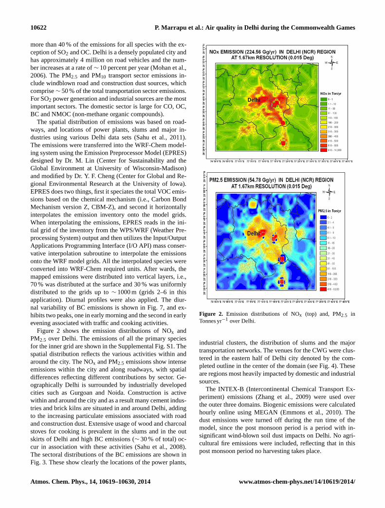
Figure 9. Spatial distributions of sector contributions to period mean surface BC concentrations.

maximum station means of 28 and 139, respectively, whilethe station minima and maxima NO and NO2 are 14 and 93,and 14 and 42, respectively. The mean daytime (9.30 a.m.to 6.30 p.m. IST) ozone value is 54.5 ppb, with station mini-mum and maximum values of 45 and 61 ppb.

The predicted distributions of these gases are also plottedin Fig. 6. Comparison with the observations shows that COis under predicted and NOx is over predicted. Ozone pre-dictions are biased high, and with a much different distribu-tion. The smaller variability among the observation sites isalso captured in the predicted values of ozone and can beexplained by looking at the spatial distribution of predicteddaytime average surface O3 in Delhi (Fig. 5b). The monitor-ing sites are all located in the eastern half of Delhi city (seeFig. 4). The ozone surface concentrations show a broaderdistribution over this domain than PM with weaker gradi-ents. Due to the rapid increase in traffic, ozone is becom-ing a more important problem with hourly observed and pre-dicted values exceeding 100 ppb (the India National AmbientAir Quality Standards (NAAQS) for 8 h average is 50 ppb(100 µg m−3); Central Pollution Control Board (CPCB) Re-port, 2012).

A sensitivity simulation was performed where NOx emis-sions were reduced to 1 / 3rd of the original values in orderto see the effects on the ozone distributions. These results forozone are also plotted in Fig. 6. Under the reduced NOx emis-

sion case the ozone distribution is much closer to that ob-served, as are the distributions of NOx and NO and NO2 (notshown). However the NOx reduction is too large, as the ozonemaximum values are overpredicted and the relative amountsof NO and NO2 are now too low and high, respectively. Theemissions are discussed in more detail in Sect. 3.4.

3.3 Sector contributions

We estimated the emission sector contributions to surfacepollution levels in Delhi. Additional model runs were per-formed to isolate the contribution from specific sectors. Fourdifferent simulations were performed. An initial run was car-ried out to calculate the total pollution from all sources; i.e.,anthropogenic, biogenic and biomass burning. Then individ-ual runs were carried out to estimate the concentrations fromeach anthropogenic sector. The equations below explain theprocess for how the transportation sector results were deter-mined.

Anthropogenic (A) = Transportation (T) + Power (P)+ (1)

Industry (I ) + Domestic (D)

Initialrun = I (A + Biogenic+ Biomass Burning+ Boundary) (2)

Individual run w/o Transport Sector

S = (A−T +Biogenic+Biomass Burning+Boundary) (3)

Atmos. Chem. Phys., 14, 10619–10630, 2014 www.atmos-chem-phys.net/14/10619/2014/

P. Marrapu et al.: Air quality in Delhi during the Commonwealth Games 10627

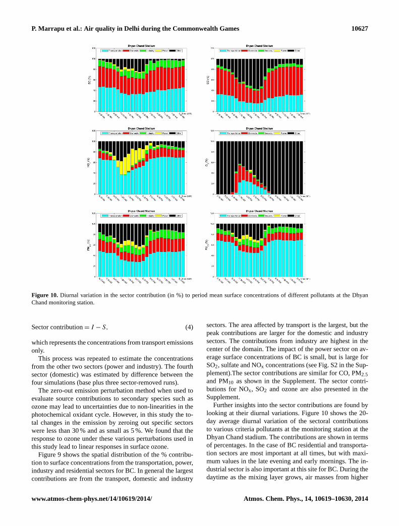
Figure 10. Diurnal variation in the sector contribution (in %) to period mean surface concentrations of different pollutants at the DhyanChand monitoring station.

Sector contribution= I − S, (4)

which represents the concentrations from transport emissionsonly.

This process was repeated to estimate the concentrationsfrom the other two sectors (power and industry). The fourthsector (domestic) was estimated by difference between thefour simulations (base plus three sector-removed runs).

The zero-out emission perturbation method when used toevaluate source contributions to secondary species such asozone may lead to uncertainties due to non-linearities in thephotochemical oxidant cycle. However, in this study the to-tal changes in the emission by zeroing out specific sectorswere less than 30 % and as small as 5 %. We found that theresponse to ozone under these various perturbations used inthis study lead to linear responses in surface ozone.

Figure 9 shows the spatial distribution of the % contribu-tion to surface concentrations from the transportation, power,industry and residential sectors for BC. In general the largestcontributions are from the transport, domestic and industry

sectors. The area affected by transport is the largest, but thepeak contributions are larger for the domestic and industrysectors. The contributions from industry are highest in thecenter of the domain. The impact of the power sector on av-erage surface concentrations of BC is small, but is large forSO2, sulfate and NOx concentrations (see Fig. S2 in the Sup-plement).The sector contributions are similar for CO, PM2.5and PM10 as shown in the Supplement. The sector contri-butions for NOx, SO2 and ozone are also presented in theSupplement.

Further insights into the sector contributions are found bylooking at their diurnal variations. Figure 10 shows the 20-day average diurnal variation of the sectoral contributionsto various criteria pollutants at the monitoring station at theDhyan Chand stadium. The contributions are shown in termsof percentages. In the case of BC residential and transporta-tion sectors are most important at all times, but with maxi-mum values in the late evening and early mornings. The in-dustrial sector is also important at this site for BC. During thedaytime as the mixing layer grows, air masses from higher

www.atmos-chem-phys.net/14/10619/2014/ Atmos. Chem. Phys., 14, 10619–10630, 2014

10628 P. Marrapu et al.: Air quality in Delhi during the Commonwealth Games

Figure 11.20 day mean contributions of pollutants from outside source.

altitudes, which are impacted by sources outside of Delhi,are entrained into the boundary layer, and the contributionfrom this process is shown by the black shading. These othercontributions are from emissions that are outside of the in-nermost grid and are transported into this region through theboundaries. PM2.5 and PM10 sector plots are similar to BC,with PM2.5 showing a larger contribution from the residentialsector than PM10, and PM10 showing a larger contributionfrom transport, which includes the contribution from courseparticles from paved and unpaved roads. CO shows a largercontribution from the domestic sector and much larger day-time contribution from distant sources, which is expected dueto the much longer lifetime of CO in the atmosphere than BC.In the case of NOx, the transport sector dominates; accept forthe daytime periods, where other sources become important.During the daytime, the power sector also contributes to sur-face concentrations as the growing mixed layer entrains theNOx emissions from nearby power plants. During the night-time the power plant plumes are above the mixed layer andare decoupled from the surface. Ozone has the largest con-tributions from sources outside of Delhi. This is shown moreclearly in spatial plots of the contributions of outside the do-main sources to the mean surface concentrations (Fig. 11).

Within Delhi the outside sources are important and contributefrom 20 to 50 % depending on species. This has importantimplications for control strategies and indicates the need forregional perspectives.

3.4 Evaluation of emissions

The comparisons of the observations and predictions for eachspecies were discussed earlier. Comparison of the correla-tions between different species can provide further informa-tion to help evaluate the emissions inventory. Illustrative re-sults are shown in Fig. 12, where plots of hourly surface ob-servations from all the sites combined are presented. The ob-servations show good correlations between BC and CO, NOxand CO, PM10 and BC, and PM2.5 and PM10. Also shown arethe same correlations based on the modeled surface concen-trations. If the model is perfect and the emission estimatesare accurate, then the correlations between the modeled con-centrations should be the same as those for the observed con-centrations. The model values also show strong correlation,with higher species-species correlation coefficients than theobservations. The PM2.5 to PM10 and the PM2.5 to BC slopesare similar for the observations and the model concentra-tions. However absolute concentrations are over predicted.

Atmos. Chem. Phys., 14, 10619–10630, 2014 www.atmos-chem-phys.net/14/10619/2014/

P. Marrapu et al.: Air quality in Delhi during the Commonwealth Games 10629

Figure 12.Comparison of correlations between different species for all the sites combined based on observations and modeled concentrations.

This suggests that the emissions are overestimated. In con-trast, the NOx-to-CO modeled slope is too high, while theconcentrations of NOx and CO are over and under predicted,respectively. This suggests that the NOx emissions are toohigh and the CO emissions too low. Assuming that the ob-servations at these sites are representative and that all themodel errors are associated with the emissions, then to makethe modeled concentrations and slopes consistent with theobserved values the emissions need to be scaled by the fol-lowing: 0.6 for NOx, 2 for CO, and 0.7 for BC, PM2.5 andPM10. The emission estimates for particles are remarkablygood considering the wide spread of activities and technolo-gies taking place in Delhi and the rapid rates of change.

4 Conclusions

Stimulated by the CWG an air quality monitoring and fore-casting system was established for Delhi. The monitoringprogram included 11 sites, which were instrumented to ob-tain continuous measurements of BC, PM2.5, PM10, O3 NOand NO2. The air quality of Delhi during the CWG had highlevels of particles with mean values of PM2.5 and PM10 at thevenues of 111 and 238 µg m−3, respectively. BC accountedfor ∼ 10 % of the PM2.5 mass. The model predictions wereevaluated using the surface observations of meteorological

parameters and the air pollution concentrations. The modelshowed a dry bias (under prediction in RH by∼ 10 %),slightly under predicted peak day time temperatures by 1–2◦

(∼ 5 %), and was biased high in wind speed. The model cap-tured the low wind speeds, but the observations often wereless than 1 m s−1, which the model estimates at 1–3 m s−1.BC, PM2.5 and PM10 were over-predicted by∼ 25 %. Thediurnal variations were well captured, with both the observa-tions and the modeled values showing nighttime maxima anddaytime minima. The daytime values compared well with theobservations, but the nighttime values were over predicted,suggesting that the nighttime mixing height and/or nighttimedispersion were under predicted. Further work is needed toevaluate the mixing heights in Delhi for day and nighttimeperiods.

A new emissions inventory was developed to support thisnew air quality forecasting initiative. The emission inventorywas evaluated by comparing the correlations in the obser-vations (e.g., BC : CO; BC : PM2.5; PM2.5 : PM10). The pre-dicted PM2.5 to PM10 and the PM2.5 to BC slopes were simi-lar to the observation-based slopes. However absolute con-centrations were over predicted, suggesting that the emis-sions are overestimated. In contrast the NOx-to-CO modeledslope was too high, while the concentrations of NOx and COwere over and under predicted, respectively. This suggest thatthe NOx emissions are too high and the CO emissions too

www.atmos-chem-phys.net/14/10619/2014/ Atmos. Chem. Phys., 14, 10619–10630, 2014

10630 P. Marrapu et al.: Air quality in Delhi during the Commonwealth Games

low. Assuming that the observations at these sites are rep-resentative and that all the model errors are associated withthe emissions, then the modeled concentrations and slopescan be made consistent by scaling the emissions by the fol-lowing: 0.6 for NOx, 2 for CO, and 0.7 for BC, PM2.5 andPM10. The emission estimates for particles are remarkablygood considering the uncertainty in the estimates due to thediverse spread of activities and technologies that take place inDelhi and the rapid rates of change. A more complete evalu-ation of the modeling system and the emissions would bene-fit from additional observations including speciated NMOC,which would allow a more thorough evaluation of the photo-chemical oxidant cycle and ozone production.

The contribution of various emission sectors includingtransportation, power, domestic and industry to surface con-centrations were also estimated. Transport, domestic and in-dustrial sectors all make significant contributions to PM lev-els in Delhi, and the sectoral contributions vary spatiallywithin the city. The transport sector is the main sector forozone. Ozone levels in Delhi are already elevated, withhourly values sometimes exceeding 100 ppb. The continuedgrowth of the transport sector is expected to make ozone pol-lution a more pressing air pollution problem in Delhi. Thecontribution for sources outside of Delhi on Delhi air qualitywas also estimated and was shown to vary spatially through-out the domain. The smallest contributions were found inthe center of the domain, where on average the contributionsranged from∼ 25 % for BC and PM to∼ 60 % for day timeozone. The sector analysis provides useful inputs into thedesign of strategies to reduce air pollution levels in Delhi.The significant contributions from non-Delhi sources indi-cates that in Delhi (as has been shown elsewhere) that thesestrategies will also need a more regional perspective.

The air quality activities established to support the CWGhave been made operational, and the monitoring sites havebeen relocated to provide better spatial representation. Anal-ysis of the 2-year time series of these observations will be thesubject of a future paper.

The Supplement related to this article is available onlineat doi:10.5194/acp-14-10619-2014-supplement.

Acknowledgements.This research was supported in part throughthe NSF EaSM program (#1049140) and the USEPA STAR Grantprogram (##y RD-83503701-0). The Indian Institute of Tropicalmeteorology, Pune, is supported by the Ministry of Earth Science,Government of India.

Michael Decker and Martin G. Schultz at The European Centrefor Medium Weather Forecasts (ECMWF), Monitoring Atmo-spheric Composition and Climate (MACC) provided the chemicalboundary conditions.

Edited by: C. H. Song

References

CPCB Report, National Ambient Air Quality Status & Trends inIndia-2010, PR Division, Central Pollution Control Board, 2012.

Drimal, M., Lewis, C., and Abianova, F.: Health Risk Assessmentto Environmental Exposure to Malodorous sulfur Coumpoundsin Central Slovakia, Carpath. J. Earth Env., 15, 119–126, 2010.

Emmons, L. K., Walters, S., Hess, P. G., Lamarque, J.-F., Pfister,G. G., Fillmore, D., Granier, C., Guenther, A., Kinnison, D.,Laepple, T., Orlando, J., Tie, X., Tyndall, G., Wiedinmyer, C.,Baughcum, S. L., and Kloster, S.: Description and evaluation ofthe Model for Ozone and Related chemical Tracers, version 4(MOZART-4), Geosci. Model Dev., 3, 43–67, doi:10.5194/gmd-3-43-2010, 2010.

Ghude, D. S., Jain, L. S., Arya, C. B., Beig, G., Ahammaed, N.Y., Kumar, A., and Tyagi, B.: ozone in ambeint air at a tropi-cal megacity Delhi: Characteristics trends and cumulative ozoneexposure indicies, J. Atmos. Chem., 60, 37–252, 2008.

Grell, A. G., Peckha, E. S., Schmitz, R., McKeen, A. S., Frost, G.,Skamarock, C. W., and Eder B.: Fully coupled online chemistrywithin the WRF model, Atmos. Environ., 39, 6957–6975, 2005.

Guttikunda, S. K., Tang, Y., Carmichael, G. R., Kurata, G., Pan,L., Streets, D. G., Woo, J.-H., Thongboonchoo, N., and Fried,A.: Impacts of Asian Megacity Emissions on Regional AirQuality during Spring 2001, J. Geophys. Res., 110, D20301,doi:10.1029/2004JD004921, 2005.

IPCC, 2007: Climate Change, 2007: The Physical Science Basis,Contribution of Working Group I to the Fourth Assessment Re-port of the Intergovernmental Panel on Climate Change, editedby: Solomon, S., Qin, D., Manning, M., Chen, Z., Marquis, M.,Averyt, B. K., Tignor, M., and Miller, L. H., Cambridge Uni-versity Press, Cambridge, United Kingdom, and New York, NY,USA, 996 pp., 2007.

Mohan, M. and Kandya, A.: An Analysis of the Annual and Sea-sonal Trends of Air Quality Index of Delhi, Environ. Monit. As-sess., 131, 267–277, 2007.

Mohan, M., Dagar, L., and Gurjar, R. B.: Preparation and Valida-tion of Gridded Emission Inventory of Criteria Air Pollutants andIdentification of Emission Hotspots for Megacity Delhi, Environ.Monit. Assess., 130, 323–339, 2006.

Ramanathan, V. and Carmichael, G.: Global and Regional ClimateChange Due to Black Carbon, Nat. Geosi., 1, 221–227, 2008.

Sahu, S. K., Beig, G., and Sharma,C.: Decadal Growth of BlackCarbon Emissions in India, Geophys, Res. Lett., 35, L02807,doi:10.1029/2007GL032333, 2008.

Sahu, S. K., Beig, G., and Parkhi , N .: Emission Inventory of An-thropogenic Pm2.5 and PM10 in Delhi during CommonwealthGames 2010, Atmos. Environ., 45, 6180–6190,2011.

Zaveri, R. A., Easter, R. C., Fast, J. D., and Peters, L. K.: Model forSimulating Aerosol Interactions and Chemistry (MOSAIC), J.Geophys. Res., 113, D13204, doi:10.1029/2007JD008782, 2008.

Zhang, Q., Streets, D. G., Carmichael, G. R., He, K. B., Huo, H.,Kannari, A., Klimont, Z., Park, I. S., Reddy, S., Fu, J. S., Chen,D., Duan, L., Lei, Y., Wang, L. T., and Yao, Z. L.: Asian emis-sions in 2006 for the NASA INTEX-B mission, Atmos. Chem.Phys., 9, 5131–5153, doi:10.5194/acp-9-5131-2009, 2009.

Atmos. Chem. Phys., 14, 10619–10630, 2014 www.atmos-chem-phys.net/14/10619/2014/