Air Pollution lecture notes
68
5R18: Environmental Fluid Mechanics Pollution dispersion in the environment 1 5R18: ENVIRONMENTAL FLUID MECHANICS AND AIR POLLUTION Dispersion of Pollution in the Atmospheric Environment “Air and water, the two essential fluids on which all life depends, have become global garbage cans” “Mankind has probably done more damage to the Earth in the 20th century than in all of previous human history” (Jacques Yves Cousteau, 1910-1997) Prof. E. Mastorakos Hopkinson Lab Tel: 32690 E-mail: [email protected]
Transcript of Air Pollution lecture notes

5R18: Environmental Fluid Mechanics Pollution dispersion in the environment
1
5R18:
ENVIRONMENTAL FLUID MECHANICS AND AIR POLLUTION
Dispersion of Pollution in the Atmospheric Environment
“Air and water, the two essential fluids on which all
life depends, have become global garbage cans”
“Mankind has probably done more damage to the
Earth in the 20th century than in all of previous human
history”
(Jacques Yves Cousteau, 1910-1997)
Prof. E. Mastorakos
Hopkinson Lab
Tel: 32690
E-mail: [email protected]
5R18: Environmental Fluid Mechanics Pollution dispersion in the environment
2

5R18: Environmental Fluid Mechanics Pollution dispersion in the environment
3
Table of Contents
1. Introduction
2. Atmospheric structure, chemistry and pollution
3. Statistical description of turbulent mixing and reaction
4. Air Quality Modelling and Plume Dispersion
5. Turbulent reacting flows and stochastic simulations
6. Summary and main points

5R18: Environmental Fluid Mechanics Pollution dispersion in the environment
4
1. Introduction
1.1 The problem
About 90% of the world’s energy comes from fossil fuels. Energy is needed for transport
(land, sea, air), electricity generation, heating in buildings and industrial processes (e.g. iron, steel,
aluminium, paper, cement manufacture). Combustion occurs in boilers, refineries, glass melters,
drying kilns, incinerators, industrial ovens and is also used to generate energy from biomass (e.g.
from wood, straw, organic waste). Burning fossil fuels, however, may result in environmental
pollution. There are many other sources of air pollution. The chemical industry (e.g. hydrocarbon
vapours, freon, sulphur oxides), metallurgy (particulates), refineries, and even the domestic
environment (e.g. particles from cooking, solvents in paint and varnishes) are just a few. Apart from
emissions in the air, we also have pollution of the aqueous environment (sea, lakes, rivers) from
industrial discharges, municipal waste (e.g. in landfills) and oil spills. The amount of pollutants
emitted from all sources is strictly regulated by legislation in most of the developed world and
forms the topic of political discussion and affects economic decisions. More pollutants are added to
the list every year and their effects on human health come under increasing scrutiny.
In most environmental pollution problems, the pollutant is released to the environment by
the, almost always, turbulent flow of a carrier fluid. The pollutant mixes with the surrounding fluid
(air or water) and undergoes chemical transformations. A proper account of “where the pollutant
went” and “what happened to it” necessitates a theory of turbulent reacting flows, i.e. the
simultaneous treatment of mixing and chemical reactions.
Due to the complexity of this topic, in this course we will discuss a little of turbulent
mixing, a little of atmospheric pollution reactions, and we will just touch on how the two
phenomena may be treated together. In doing so, we will also touch on the extremely important
field of Air Quality Modelling, which is an interdisciplinary fields borrowing elements from Fluid
Mechanics, Atmospheric Chemistry, Meteorology and others.
1.2 Objectives
The objectives of this series of lectures are:
To present the nature of atmospheric pollution.
To present commonly used pollutant dispersion models.
To make the student familiar with the topic of Air Quality Modelling.
To introduce the necessity to study turbulent reacting flows.
To introduce techniques for simulating turbulent reacting flows.
At the end of the lectures, the student should:
Be able to make simple estimates of the amounts of pollutant reaching a given point far
away from a pollution source.
Understand how the local meteorology may affect pollutant dispersion.
Understand some of the physics of turbulent mixing.
Be able to estimate how the turbulence may affect the rate of pollutant transformation.
Be familiar with techniques and software used in practical Air Quality Modelling.
Be able to design a Monte-Carlo simulation for stochastic phenomena.

5R18: Environmental Fluid Mechanics Pollution dispersion in the environment
5
1.3 Structure of this course
These lecture notes are organized as follows: elements of chemical kinetics, the nature of
atmospheric pollutants and a little atmospheric chemistry are discussed in Chapter 2. In Chapter 3, a
description of the fundamentals of turbulent mixing is given. In Chapter 4, the model problem of
dispersion of a chimney plume is discussed in detail. Chapter 5 presents some usual theories for
turbulent reacting flows and emphasizes the use of Monte Carlo techniques to overcome the closure
problems introduced by the turbulence. Although it is not crucial, we will be mostly considering
gaseous flows.
Simple computational codes of the type used in Air Quality Modelling for decision-making
will be demonstrated and the assumptions behind them will be fully discussed.
1.4 Bibliography
Csanady, G. T. (1973) Turbulent Diffusion in the Environment. Reidel Publishing Company.
Chapter 3 is one of the classics in the field of turbulent mixing and goes deep in the physics
involved and describes well the applications. Very useful for our Chapter 4.
De Nevers, N. (1995) Air Pollution Control Engineering. McGraw Hill.
Discusses various features of air pollution engineering (pollution control techniques, NOx
chemistry, plume dispersion). Very useful for Chapters 2 and 4 of this course. Highly
recommended and a very good addition to any engineer’s library.
Jacobson, M. Z. (1999) Fundamentals of Atmospheric Modelling. Cambridge University Press.
Discusses various features of air pollution and the current generation of atmospheric
dispersion codes. Chapter 11 (pp. 298-307) is very useful for the various harmful effects of air
pollution and the species that participate in smog formation and Ch. 2 (pp. 6-20) for the
atmospheric structure. For those who like chemistry and who want to follow Air Quality
Modelling as a profession.
Pope, S.B. (2000) Turbulent Flows. Cambridge University Press.
Not for the faint-hearted! Chapter 3 describes in detail the pdf approach of turbulence, while
Chapter 12 gives the full Monte Carlo treatment for turbulent flows. PhD level.
Tennekes and Lumley (1972) An Introduction to Turbulence. MIT Press.
Chapter 1 from this book is one of the best introductions to turbulence available and you
should read it. Chapter 6 gives the probabilistic description of turbulence. Both chapters are
recommended, but you may avoid the difficult mathematical bits of chapter 6.

5R18: Environmental Fluid Mechanics Pollution dispersion in the environment
6
2. Atmospheric structure, chemistry and pollution
In this Chapter, we will give a quick revision of terms and concepts from chemical kinetics,
which are needed to allow us to use and understand atmospheric chemistry. Some particular
features of pollution chemistry then follow and information on the structure of the atmosphere is
given.
2.1 Fundamental concepts – revision of chemistry
Mole and mass fractions, concentrations
Assume that pollutant A reacts with species B, which could be another pollutant or a
background species (e.g. N2, O2, H2O in the air). The reaction rate depends on the amount of
reactant present. There are many ways to quantify the amount of a species in a mixture:
concentration, mole (or volume) and mass fractions are the most usual. The ratio of the number of
kmols, ni, of a particular species i to the total number of kmols ntot in the mixture is the mole
fraction or volume fraction:
tot
ii
n
nX . (2.1)
The mass fraction Yi is defined as the mass of i divided by the total mass. Using the obvious
111
N
ii
N
ii YX , (2.2)
where N is the total number of species in our mixture, the following can be easily derived for Yi and
the mixture molecular weight MW :
MW
MWXY i
ii , (2.3)
1
11
N
i i
iN
iii
MW
YMWXMW . (2.4)
Virtually always, the mixture molecular weight will be very close to that of air since the pollutant is
dilute (i.e. even if it is heavy, its contribution to the weight of a kmol of mixture is very small).
Equation (2.4) is included here only for completeness.
The concentration (or molar concentration) of species i is defined as the number of kmols
of the species per unit volume. The usual notation used for concentrations is Ci or the chemical
symbol of the species in square brackets, e.g. [NO] for nitric oxide, or [A] for our generic pollutant
A. From this definition and Eq. (2.1),
V
nX
V
nC totii
i , (2.5)
and using the equation of state PV=ntotR0T (R
0 is the universal gas constant), we get:

5R18: Environmental Fluid Mechanics Pollution dispersion in the environment
7
TR
PX
PTRn
nXC i
tot
totii 00 /
(2.6)
This relates the concentration to the mole fraction. In most atmospheric pollution problems, the
concentrations are quoted in molecules/m3 or kmol/m
3 and the volume fractions in parts per billion
(ppb). A very common unit is kg of pollutant per m3 of air, which is the molar concentration times
the molecular weight of the species. We can also relate the concentration to the mass fraction:
i
i
i
ii
MW
Y
TR
P
MW
MWYC
0. (2.7)
where is the mixture density, e.g. the air density for our problems. Usually, the chemical reaction
rate is expressed in terms of molar concentrations, while the conservation laws for mass and energy
are expressed in terms of mass fractions. On the other hand, pollution monitoring equipment
measures usually the volume fractions or the kg/m3 of the pollutant. The above relations are useful
for performing transformations between the various quantities, which is very often needed in
practice.
Global and elementary reactions
Chemical reactions occur when molecules of one species collide with molecules of another
species and, for some of these collisions, one or more new molecules will be created. The chemical
reaction essentially involves a re-distribution of how atoms are bonded together in the molecule. To
achieve this, chemical bonds must be broken during the impact (i.e. the molecules must have
sufficient kinetic energy) and other bonds must be formed. As the energy of these bonds depends on
the nature of the atoms and on geometrical factors, the energy content of the products of the
collision may be different from the energy content of the colliding molecules. This is the origin of
the heat released (or absorbed) in chemical reactions.
We write often that, for example, methane is oxidised according to CH4+2O2CO2+2H2O.
This is an example of a global reaction. What we mean is that the overall process of oxidation uses
1 kmol of CH4 and 2 kmol of O2 to produce, if complete, 1 kmol of CO2 and 2 kmol of H2O. We do
not mean that all this occurs during an actual molecular collision. This would be impossible to
happen because it would involve too many bonds to break and too many bonds to form. However,
the reactions
CH4 + O CH3 + OH
O3 + NO NO2 + O
NO + OH + M HNO2 + M
are possible. For example, the first of these involves breaking one C-H bond and forming a O-H
one. These reactions are examples of elementary reactions, i.e. reactions that can occur during a
molecular collision. The overall chemical transformation follows hundreds or thousands of such
elementary reactions and many species and radicals appear. By the term “radicals” we mean very
reactive unstable molecules like O, H, OH, or CH3. The series of elementary reactions that
describes the overall process is called a reaction mechanism or detailed chemical mechanism. Most
chemical transformations occur following reaction mechanisms, rather than single reactions.
The concept of global reaction helps us visualize the overall process and stoichiometry in an
engineering sense. But when we identify the elementary reactions we can talk in detail about what
really happens.
5R18: Environmental Fluid Mechanics Pollution dispersion in the environment
8
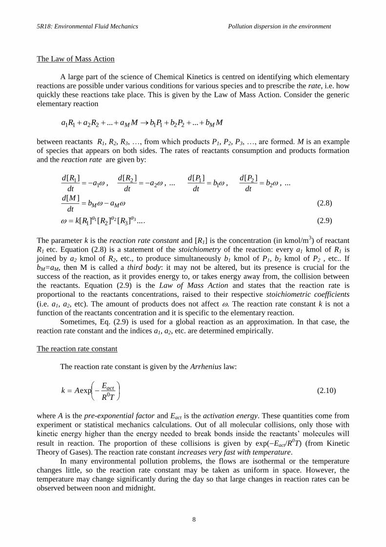
The Law of Mass Action
A large part of the science of Chemical Kinetics is centred on identifying which elementary
reactions are possible under various conditions for various species and to prescribe the rate, i.e. how
quickly these reactions take place. This is given by the Law of Mass Action. Consider the generic
elementary reaction
MbPbPbMaRaRa MM ...... 22112211
between reactants R1, R2, R3, …, from which products P1, P2, P3, …, are formed. M is an example
of species that appears on both sides. The rates of reactants consumption and products formation
and the reaction rate are given by:
... , ][
, ][
22
11 a
dt
Rda
dt
Rd ... ,
][ ,
][2
21
1 bdt
Pdb
dt
Pd
MM abdt
Md
][ (2.8)
...][][][ 321321
aaa RRRk . (2.9)
The parameter k is the reaction rate constant and [R1] is the concentration (in kmol/m3) of reactant
R1 etc. Equation (2.8) is a statement of the stoichiometry of the reaction: every a1 kmol of R1 is
joined by a2 kmol of R2, etc., to produce simultaneously b1 kmol of P1, b2 kmol of P2 , etc.. If
bM=aM, then M is called a third body: it may not be altered, but its presence is crucial for the
success of the reaction, as it provides energy to, or takes energy away from, the collision between
the reactants. Equation (2.9) is the Law of Mass Action and states that the reaction rate is
proportional to the reactants concentrations, raised to their respective stoichiometric coefficients
(i.e. a1, a2, etc). The amount of products does not affect . The reaction rate constant k is not a
function of the reactants concentration and it is specific to the elementary reaction.
Sometimes, Eq. (2.9) is used for a global reaction as an approximation. In that case, the
reaction rate constant and the indices a1, a2, etc. are determined empirically.
The reaction rate constant
The reaction rate constant is given by the Arrhenius law:
TR
EAk act
0exp (2.10)
where A is the pre-exponential factor and Eact is the activation energy. These quantities come from
experiment or statistical mechanics calculations. Out of all molecular collisions, only those with
kinetic energy higher than the energy needed to break bonds inside the reactants’ molecules will
result in reaction. The proportion of these collisions is given by exp(Eact/R0T) (from Kinetic
Theory of Gases). The reaction rate constant increases very fast with temperature.
In many environmental pollution problems, the flows are isothermal or the temperature
changes little, so the reaction rate constant may be taken as uniform in space. However, the
temperature may change significantly during the day so that large changes in reaction rates can be
observed between noon and midnight.
5R18: Environmental Fluid Mechanics Pollution dispersion in the environment
9
2.2 Pollutants and their sources
An overview
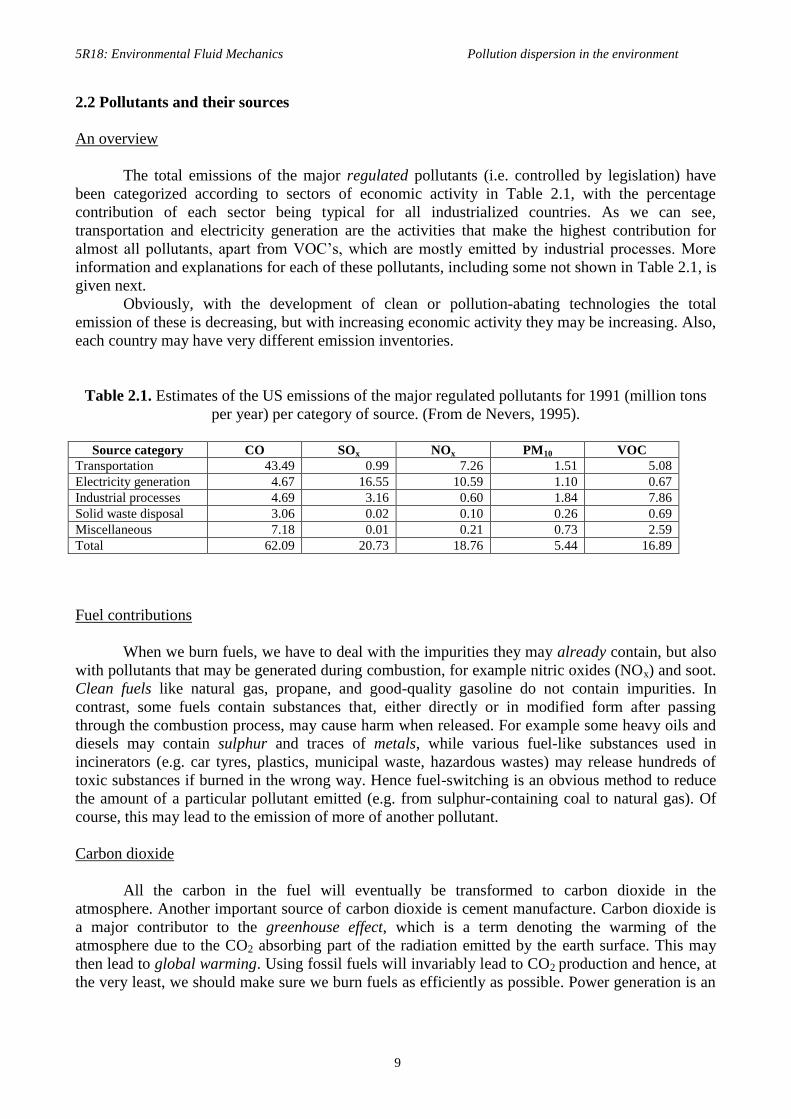
The total emissions of the major regulated pollutants (i.e. controlled by legislation) have
been categorized according to sectors of economic activity in Table 2.1, with the percentage
contribution of each sector being typical for all industrialized countries. As we can see,
transportation and electricity generation are the activities that make the highest contribution for
almost all pollutants, apart from VOC’s, which are mostly emitted by industrial processes. More
information and explanations for each of these pollutants, including some not shown in Table 2.1, is
given next.
Obviously, with the development of clean or pollution-abating technologies the total
emission of these is decreasing, but with increasing economic activity they may be increasing. Also,
each country may have very different emission inventories.
Table 2.1. Estimates of the US emissions of the major regulated pollutants for 1991 (million tons
per year) per category of source. (From de Nevers, 1995).
Source category CO SOx NOx PM10 VOC
Transportation 43.49 0.99 7.26 1.51 5.08
Electricity generation 4.67 16.55 10.59 1.10 0.67
Industrial processes 4.69 3.16 0.60 1.84 7.86
Solid waste disposal 3.06 0.02 0.10 0.26 0.69
Miscellaneous 7.18 0.01 0.21 0.73 2.59
Total 62.09 20.73 18.76 5.44 16.89
Fuel contributions
When we burn fuels, we have to deal with the impurities they may already contain, but also
with pollutants that may be generated during combustion, for example nitric oxides (NOx) and soot.
Clean fuels like natural gas, propane, and good-quality gasoline do not contain impurities. In
contrast, some fuels contain substances that, either directly or in modified form after passing
through the combustion process, may cause harm when released. For example some heavy oils and
diesels may contain sulphur and traces of metals, while various fuel-like substances used in
incinerators (e.g. car tyres, plastics, municipal waste, hazardous wastes) may release hundreds of
toxic substances if burned in the wrong way. Hence fuel-switching is an obvious method to reduce
the amount of a particular pollutant emitted (e.g. from sulphur-containing coal to natural gas). Of
course, this may lead to the emission of more of another pollutant.
Carbon dioxide
All the carbon in the fuel will eventually be transformed to carbon dioxide in the
atmosphere. Another important source of carbon dioxide is cement manufacture. Carbon dioxide is
a major contributor to the greenhouse effect, which is a term denoting the warming of the
atmosphere due to the CO2 absorbing part of the radiation emitted by the earth surface. This may
then lead to global warming. Using fossil fuels will invariably lead to CO2 production and hence, at
the very least, we should make sure we burn fuels as efficiently as possible. Power generation is an
5R18: Environmental Fluid Mechanics Pollution dispersion in the environment
10
important player in the public debate concerning global climate change. Switching to renewable
energies alleviates the danger of global warming.
Carbon monoxide
Incomplete combustion results in CO formation. Carbon monoxide is extremely dangerous
and can cause death if inhaled in large concentrations because it inhibits the acquisition of oxygen
in our blood stream. It is mostly emitted by cars (Table 2.1). The use of catalysts has helped to
reduce the problem considerably by ensuring the oxidation of CO to CO2. The trail of CO behind a
car is of interest to environmental regulation agencies and methods to predict and measure CO are
being developed.
Sulphur oxides
When burning fuels with sulphur, like coal and diesel, all of the sulphur will be oxidised
into SO2 and SO3, collectively called SOx. Other sources are processes like copper smelting.
Sulphur oxides pose serious problems because: (i) SOx dissolves in clouds to form sulphuric acid,
which can then be deposited to the earth by rain. This is called “acid rain” and has caused
deforestation in Europe and North America and serious damage to structures (monuments, steel
buildings). (ii) SOx is a respiratory irritant and in large concentrations can cause death. Sulphur-rich
coal combustion for domestic use (e.g. for cooking or heating) has been responsible for thousands
of deaths in London over the past centuries, notably during the “Great London Smog” in December
1952, in which about 4,000 people died.
Current emission standards on sulphur oxide emissions are very strict and are met by post-
combustion treatment of the exhaust gases. This is based mostly on scrubbing: mixing the exhaust
gases with water droplets that contain limestone, which reacts with the oxide according to CaCO3 +
SO2 + 0.5O2 CaSO4 + CO2. The cost of the scrubbers is a very large percentage of a modern coal
power station.
Nitrogen oxides
Two of the most serious pollutants attributed to fossil fuel usage are nitric oxide (NO) and
nitrogen dioxide (NO2), collectively called NOx. Usually, only NO is emitted, but this will react in
the atmosphere to create NO2 (Section 2.3). Other sources of nitric oxides in the atmosphere include
agriculture (fertilizer production). Nitrogen oxides will form acid rain, by a similar mechanism to
SOx. At ground level and under sunlight, NO2 will release an oxygen atom that can then form ozone
(O3) (more of this later). Ozone is very irritating for the respiratory system and causes impaired
vision. In addition, NO emitted by high-altitude airplanes participates in ozone destruction and
hence contributes to the ozone hole problem. Nitrogen oxides are strictly regulated and lowNOx
combustion equipment (burners, processes, cars, domestic heaters) has become today a huge
business.
Particulate matter and soot
Combustion without excess air may lead to soot formation. By “soot” we mean solid
particles of size less than 1m, which result in the yellow colour of flames and in the smoke emitted
from diesel engines and some older gas turbines. The particulate matter may cause lung diseases
and is hence controlled by legislation. The particulates are usually denoted by PM10, which means
“particulate matter of size less than 10m”. Other anthropogenic sources of PM10 in the atmosphere

5R18: Environmental Fluid Mechanics Pollution dispersion in the environment
11
include ash particles from coal power stations, while natural sources are salt particles from breaking
sea waves, pollen, dust, forest fires, and volcanic eruptions.
VOC
The term VOC refers to “volatile organic compounds”. By VOC we mean evaporated
gasoline from petrol filling stations, vapours from refineries, organic solvents from paint and dry
cleaning, and many others. These organic species are major contributors to smog and may be toxic
or carcinogenic for humans. Their emissions are strictly regulated. Studies have found that glues
and paints in our houses may have serious adverse health effects. There is a large effort today to
switch to water-based paint, so that emissions of VOC’s are decreased.
Heavy metals and dioxins
If metals are contained in the reactants to our process (e.g. burner, kiln, chemical reactor),
they may end up in the atmosphere (in pure form or in oxides) and they could be very dangerous
(particularly Hg, Cd, Pb, As, Be, Cr, and Sb). This is a serious problem for municipal, toxic, and
hospital waste incinerators. If the fuel contains chlorine, for example if it includes plastics (PVC),
then there is a danger that dioxins may be formed not at the flame, but on medium-temperature
metal surfaces in the stack or inside the waste itself. Dioxins are chlorinated aromatic organic
compounds whose chemistry is not very well known. They are extremely dangerous because they
are carcinogenic even in concentrations of part per trillion. Municipal waste incinerators are needed
to decrease the volume of waste going to landfills and to generate some power, but their use is
controversial because of the danger of dioxins. If the plant operates at the design point, the exhaust
is probably free of dangerous substances because a lot of attention has been given to the clean-up
stage. However, open, uncontrolled burning of any waste or plastic material is extremely dangerous.
Other sources of dioxins used to be the paper industry, where chlorine-containing compounds were
used for bleaching the pulp and ended up in the waste stream of the paper mill, but this problem
seems to have improved considerably with the introduction of new chlorine-free techniques.
2.3 Some chemistry of atmospheric pollution
Smog formation
One of the most important environmental problems is smog formation (Smoke + Fog), also
called photochemical pollution. This is the brown colour we sometimes see above polluted cities
and consists of a very large number of chemicals, but the most important are nitric oxide (NO),
nitrogen dioxide (NO2), ozone (O3), and hydrocarbons (VOC). Some of the reactions participating
in smog formation are discussed below.
Oxidation of NO to NO2
Of the two possibilities:
2NO + O2 2NO2 R-I
NO + O3 NO2 + O2 R-II
the second is about four orders of magnitude faster. Therefore, the formation of nitrogen dioxide
from the emitted NO depends on the availability of ozone.
5R18: Environmental Fluid Mechanics Pollution dispersion in the environment
12
Photolytic reactions
A very important characteristic of smog is that it requires sunlight, which causes the
photolysis of various chemicals into smaller fragments (‘photo’ = light; ‘lysis’ = breaking).
Examples of sequences of reactions triggered or followed by photolysis:
NO2 + hv O + NO R-III
O + O2 + M O3 + M R-IV
O + H2O 2OH R-V
and
NO + NO2 + H2O 2HNO2 R-VI
HNO2 + hv NO + OH R-VII
The rate of photolytic reactions is usually given by an expression equivalent to Eq. (2.10), with the
pre-exponential factor taken as a function of incident solar radiation. Hence the photolytic reaction
rates are functions of the cloud cover and latitude in a given location, in addition to the time of the
day and season. Smog is more common in sunny cities and in the summer because R-III (and other
photolytic reactions) proceeds faster.
The photostationary state
Reactions R-II, R-III and R-IV suggest the following “cycle” for ozone: R-III produces an
oxygen atom, which results in ozone formation through R-IV, which then reacts with NO in R-II. It
is a common assumption that these reactions proceed very fast compared to others in smog
chemistry and then the oxygen atom and ozone reach a quasi-steady state, called the
“photostationary state”. If we assume that d[O]/dt =0 and d[O3]/dt=0 and we use the Law of Mass
Action for the three reactions (R-II to R-IV), we get that
]NO[
]NO[]O[ 2
3II
III
k
k (2.11)
where kII and kIII are the reaction rate constants for R-II and R-III respectively. Therefore we
expect ozone (and smog) to be in high concentrations around midday when the photolytic reaction
R-III has its peak. We also expect ozone to decrease to low values at night. Both these observations
are approximately borne out by measurements. Above heavily polluted cities in the mornings, Eq.
(2.11) is not very accurate due to the presence of VOC’s, which also produce NO2, as we shall see
below. In the afternoons, when VOC’s tend to decrease due to their own photolysis, Eq. (2.11) is
not a bad approximation.
The hydrocarbons
A prerequisite for smog is the presence of hydrocarbons, collectively called VOC’s. A
global reaction describing their participation in smog formation is
NO + VOC NO2 + VOC* R-VIII
where VOC* denotes some other organic radical. The NO2 will then follow the cycle in R-II, R-III
and R-IV, which releases ozone. During the VOC chemistry, the major eye irritant CH3COO2NO2
may also appear (called peroxyacetyl nitrate or PAN). We see therefore that a combination of
5R18: Environmental Fluid Mechanics Pollution dispersion in the environment
13
nitrogen oxide emission and hydrocarbons will under the action of sunlight cause serious pollution.
The situation is worse above cities than above rural areas due to the high emissions from cars and
other activities. The chemistry of smog formation is extremely more complex than the above over-
simplified picture and is the subject of intensive research.
Acid rain
Sulphur from oils and coal is usually oxidised during combustion and is then emitted in the
form of SO2, which will react in the atmosphere according to:
SO2 + OH HSO3 R-VIII
HSO3 + O2 SO3 + HO2 R-VIII
SO3 + H2O H2SO4 R-IX
i.e. sulphuric acid is formed. This is absorbed on water droplets and may be deposited on the ground
by rain. This is the notorious “acid rain”, a term that also includes nitric acid that is similarly
formed. The situation has improved the last decade with the use of scrubbers in power stations,
which capture SO2 before it is emitted.
2.4 Some comments on the atmosphere
It is important to realize that the atmosphere at various heights behaves very differently, not
only in terms of the chemistry that takes place, but also in terms of the fluid mechanics we see.
Most pollution problems occur at the lower levels, although the ozone hole and global warming are
issues of the higher levels too. Here, we present briefly the structure of the lower atmosphere, which
will be necessary for understanding the atmospheric dispersion processes in Chapter 4.
Atmospheric structure
Pressure, temperature, “standard atmosphere”
The pressure, density, and temperature of the atmosphere are related with height through
gdz
dp (2.12)
RTp (2.13)
pc
g
dz
dT (2.14)
where R=R0/MWair. Equation (2.14) gives the Dry Adiabatic Lapse Rate (DALR) as 9.3 K/km. We
very often use the “standard atmosphere” lapse rate, an average over all seasons of the year and
across many regions of the globe, which is about 6.5 K/km. This can then be used in Eqs. (2.12) and
(2.13) to find the vertical pressure and density distribution.
The boundary layer and the troposphere, inversions
The troposphere is the first 11 km above sea level and contains 75% of the mass of the
whole atmosphere. It is usually divided into the boundary layer and the free troposphere. The
boundary layer depth ranges between 500 and 3000 m and it is divided into the surface layer (the

5R18: Environmental Fluid Mechanics Pollution dispersion in the environment
14
first 10% closest to the ground) and the neutral convective layer, also called the mixed layer. At the
top of the boundary layer, we have the inversion layer. This structure is shown on Fig. 2.1.
It is important to realize that because the ground changes temperature quicker than the air, it
affects the air immediately above it and hence the temperature locally in the surface layer may have
a different gradient than the DALR. Therefore, the vertical temperature gradient will be different
during the day and at night, which affects the stability of the layer. At night, the surface layer and a
large part of the mixed layer become stable as the temperature increases with height due to radiative
cooling of the ground.
At the top of the boundary layer, the temperature gradient is usually positive (i.e. stable) and
the turbulence dies there. This is the inversion layer. Between the inversion and the neutral layers,
we have the so-called entrainment zone, which is where we see often cloud formation. Because it is
not easy to penetrate the inversion layer, it can be considered as the ceiling of pollution. Therefore,
most of the pollution emitted at ground level will disperse approximately up to the first 3 km of the
atmosphere, with further diffusion to the free troposphere being a slower process.
Daytime Temperature
Bou
ndary
layer
Surface layer
Neutral convective
mixed layer
Free troposphere
Alt
itu
de
Entrainment zone Cloud layer
Inversion layer
3000 m
300 m
Surface layer
Neutral residual layer
Free troposphere
Entrainment zone
Inversion layer
3000 m
Stable boundary layer
Nighttime Temperature
DALR
Figure 2.1 Variation of temperature in the atmospheric boundary layer with height during day and
night (from Jacobson, 1998).
Mixing height
Figure 2.1 also serves to visualize another very important quantity in the field of
atmospheric pollution dispersion: that of the mixing height. With this we simply mean the height
above ground where the inversion occurs, which means that the turbulence dies and hence stops
mixing. So, for Fig. 2.1 during day, the mixing height would be at 3000 m.
For dawn and early morning, the situation is better visualized in Fig. 2.2, where we look at
various times progressively after sunrise. Curve A shows a stable stratification at dawn. The air is

5R18: Environmental Fluid Mechanics Pollution dispersion in the environment
15
still due to the damping effect of the stable atmosphere during the night and hence no mixing can
occur. As the ground heats up due to the sun radiation, the temperature profile becomes like that of
Curve B and the mixing height is small, say 100 m. Therefore, the first 100 m will have turbulence
and mixing can occur. As time goes on, the mixing height increases because the unstable layer close
to the ground becomes thicker. At mid or late afternoon, the mixing height has reached the
inversion layer of the atmospheric boundary layer shown in Fig. 2.1.
The fact that the mixing height changes during the day and that often no significant mixing
may be expected at night, has tremendous implications for local pollution episodes, as we will
discuss more fully in Chapter 4.
Alt
itu
de
Temperature
DALR
A
B
C
D
A: Dawn
B: Dawn + 2h
C: Dawn + 4h
D: Midafternoon
Figure 2.2 Variation of the temperature at various times during a typical morning. The mixing
height increases with time. (Adapted from De Nevers, 1995.)
2.5 Global warming
“Global warming” is a much-used (and abused) phrase. It refers to the increase in the average
temperature of the atmosphere caused by an enhanced greenhouse effect, which in turn is caused by
increased concentrations of some gases in the atmosphere. “Climate change” is a more general term
that refers to changes in the climate (which can include cooling) due to the anthropogenic
emissions. Cooling in one point of the planet may be caused by warming in another point, so a
discussion of the greenhouse effect, and how this is affected by emissions, is necessary for
understanding all these phenomena. For a nice summary, see:
http://en.wikipedia.org/wiki/Global_warming
The key scientific topic is the radiative balance in the atmosphere, which is discussed next.
Consider Fig. 2.3, which shows a planet in the path of radiation. Assume an incoming solar flux of

5R18: Environmental Fluid Mechanics Pollution dispersion in the environment
16
S (W/m2) incident on the outer layers of the atmosphere. This solar radiation is intercepted by the
planet’s projected area (R2), where R is the planet’s radius,
Assume that the surface is uniform (i.e. same radiative properties and temperature everywhere) and
let us neglect at this stage the presence of the atmosphere. Thermodynamic equilibrium implies that
the net heat falling on the surface balances the heat emitted by the surface:
R2(1-)S = 4R
2Ts
4 (2.15)
giving
Ts = [(1-)S / 4 ]1/4
(2.16)
where Ts is the surface temperature, the emissivity of the surface, the albedo (the fraction of
incident radiation that is reflected), the Stefan-Boltzmann constant (equal to 5.67108
W/m2/K
4). For Earth, the emissivity and the albedo are not constant (they depend on the nature of
the surface, whether it is covered by water, ice, vegetation etc), but some average values are 0.61
and 0.3 respectively. These effective values include the presence of the atmosphere, clouds etc.
Given that S 1367 W/m2, we get that Ts = 288 K. This is an estimate of the Earth’s average
surface temperature, in the sense of an effective radiative temperature. Eq. (2.16) also shows the
great sensitivity of the surface temperature in changes of solar radiation, albedo and emissivity; 1 K
change can be brought about by 1-2% change in these parameters. Note that the greenhouse effect
(discussed below) is already included in the effective values of emissivity and albedo.
Figure 2.3 Simplified view of Earth’s receiving radiation from the sun.
In a more detailed view, Fig. 2.4 shows the various heat exchange processes taking place between
the Earth’s surface and the incoming solar radiation (note that in this picture the solar radiation is
expressed in terms of m2 of the total Earth’s surface area). The greenhouse gases (mainly water
vapour, methane, and CO2) absorb some of the radiated heat from the surface and re-radiate it back
S
Area: R2

5R18: Environmental Fluid Mechanics Pollution dispersion in the environment
17
to the surface, which results in a warming of the surface. If there were no greenhouse gases at all,
the surface would be very cold for human life, while if their concentration increases, the re-radiated
fraction increases.
The presence of atmospheric aerosols (natural or man-made) increases the reflection of the sun’s
radiation, and therefore their presence can act so as to reduce the surface temperature. The power
generation and the transport sectors produce significant amounts of aerosols and their effect on
climate change is a very important topic of current research. More on aerosols in a later part of this
course.
Figure 2.4 Energy exchanges in the atmosphere (From the IPCC 4th
Assessment Report; “Climate
Change 2007: The Physical Basis”, CUP, 2007)
5R18: Environmental Fluid Mechanics Pollution dispersion in the environment
18
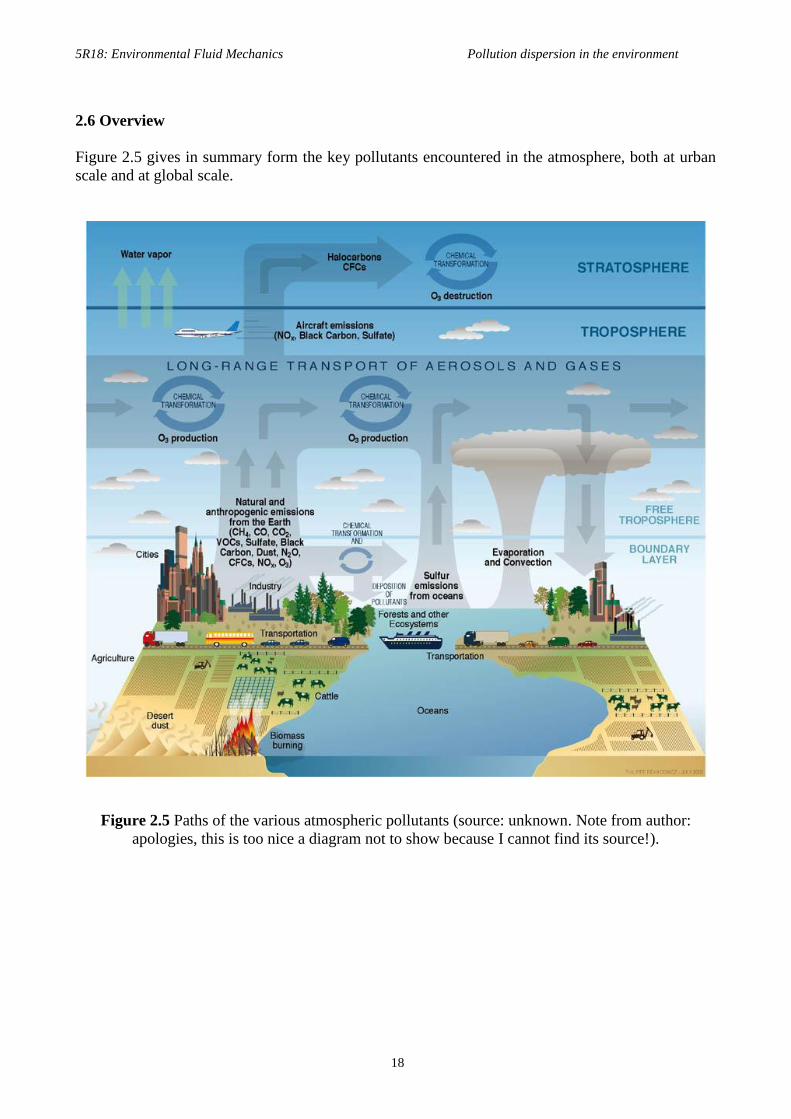
2.6 Overview
Figure 2.5 gives in summary form the key pollutants encountered in the atmosphere, both at urban
scale and at global scale.
Figure 2.5 Paths of the various atmospheric pollutants (source: unknown. Note from author:
apologies, this is too nice a diagram not to show because I cannot find its source!).

5R18: Environmental Fluid Mechanics Pollution dispersion in the environment
19
2.7 Worked Examples
Example 2.1
An air quality monitoring station measured one early morning that the volume fractions of
NO, ozone and NO2 were 30, 40, and 170 ppb respectively. What were the corresponding
concentrations in kmol/m3, in molecules/m
3, and in kg/m
3? The atmospheric conditions at the time
of the measurement were 980 mbar pressure and 10ºC temperature.
Solution
From Eq. (2.6), TRPXC ii0/ , and using P=0.98x10
5 Pa, T=283 K, R
0=8315 J/kmol/K,
we get that NOC 30x109
x 98x103
/ (8315 x 283) = 1.24 x10⁹
kmol/m3. Note that the 30 ppb
becomes a volume fraction of 30x109
. Similarly for the other species. To transform the kmol/m3
into molecules/m3, we need to multiply by Avogadro’s Number, 6.022x10
26 molecules/kmol. To get
the concentration in kg/m3, we multiply the molar concentration by the molecular weight of the
species.
Example 2.2
Estimate the mass of the air in the atmospheric boundary layer, assuming a total height of 3
km and a linear reduction of temperature with height of 6.5 K/km (the “standard atmosphere”) from
a mean ground-level temperature of 288 K.
Solution
The standard atmosphere gives that zTzT 5.6)0()( , where z is measured in km and
T(0)=288K. The total mass of the air M(z) in the atmosphere up to a height z per unit area is given
by z
dzzM
0
)( . Writing adzdT / and using the hydrostatic balance equation gdzdP / ,
differentiation of the equation of state RTp gives:
dzRdTdzRTddzdp /// RagdzRTd /azT
dz
R
gaRd
)0(
)0(
)0(ln
)0(
)(ln
T
azT
aR
aRgz
1
)0(
)0()0()(
aR
g
T
azTz . So at z=3 km, the density of
air is 0.9 kg/m3 and the temperature 268.5 K (4.5 C). The density variation can now be integrated
to give:
1 , )()0()0(
)0(
1
1)( 11
0
aR
gmzTT
aTmdzzM mm
m
z
.
With a=6.5 K/km and z=3 km, the total mass per unit area becomes 3143.7 kg/m2. Note that
if we had used the average value between [(0)+(3km)]/2 we would have obtained a mass per unit
area of 3160.5 kg/m2. The fact that this estimate is so good reflects the fact that inside the boundary
layer the density changes almost linearly with height (but not outside it).
To find the total mass, we must multiply by the surface area of the Earth, which is 4Rearth2,
and this gives a total mass in the boundary layer of 1.6x10¹⁸
kg. This corresponds to about 30% of
the mass of the whole atmosphere.
5R18: Environmental Fluid Mechanics Pollution dispersion in the environment
20
Example 2.3
Assume that the average car emits 0.2 kg CO2 per km driven. The average user drives
10,000 km per year and there are about 450,000,000 cars in the world today. Estimate the yearly
increase of CO2 in the atmosphere in ppb due to car emissions.
Solution
The total CO2 released per year from all cars is 0.2 x 10,000 x 450,000,000=9x10¹¹
kg per
year. From Example 2.2, the total atmospheric mass will be 1.6x10¹⁸
/0.3=5.3x1018
kg. Then the
volume fraction of CO2 will be from Eq. (2.3): XCO2=YCO2 x (29/44) = (9x10¹¹
/5.3x1018
) x (29/44),
i.e. 112 ppb increase per year.
The measured increase in CO2 concentration in the atmosphere is about 1100 ppb per year
(Jacobson, 1998). This includes power generation, industry and land use. Figures including the
whole of the transport sector (e.g. buses, trucks, trains etc.) and with more exact values for the
average mileage and CO2 emitted per vehicle give that the contribution of transport is about 24% of
the CO2 releases, which is estimated to be a total of 6.2x10¹²
kg/year.
5R18: Environmental Fluid Mechanics Pollution dispersion in the environment
21
3. Statistical description of turbulent mixing
In this Chapter, we will derive the governing equation for a reacting scalar in a turbulent
flow and we will demonstrate why the turbulence affects the mean reaction rate. We will also
present concepts from probability theory that are useful for understanding why the concentration
fluctuations are important in environmental pollution and for providing measures to describe these.
The material here is needed background for understanding the practical Air Quality Modelling
techniques introduced in later Chapters.
3.1 Governing equation for a reacting scalar
Conservation of mass
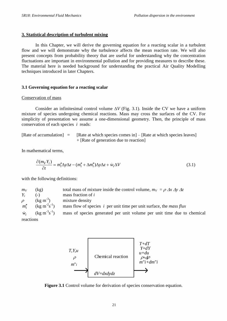
Consider an infinitesimal control volume V (Fig. 3.1). Inside the CV we have a uniform
mixture of species undergoing chemical reactions. Mass may cross the surfaces of the CV. For
simplicity of presentation we assume a one-dimensional geometry. Then, the principle of mass
conservation of each species i reads:
[Rate of accumulation] = [Rate at which species comes in] – [Rate at which species leaves]
+ [Rate of generation due to reaction]
In mathematical terms,
Vwzymmzymt
Ymiiii
iV
)(
)( (3.1)
with the following definitions:
mV (kg) total mass of mixture inside the control volume, mV = x y z
Yi (-) mass fraction of i
(kg m-3
) mixture density
im (kg m-2
s-1
) mass flow of species i per unit time per unit surface, the mass flux
iw (kg m-3
s-1
) mass of species generated per unit volume per unit time due to chemical
reactions
T,Y,u
m"i
dV=dxdydz
Chemical reaction
T+dT Y+dY u+du
m"i+dm"i +d
Figure 3.1 Control volume for derivation of species conservation equation.

5R18: Environmental Fluid Mechanics Pollution dispersion in the environment
22
Letting x go to zero, we obtain the species conservation equation:
iii w
x
m
t
Y
)( (3.2)
Equation (3.2) is a partial differential equation (in time and space) and to be in a position to solve it,
we need expressions for the mass flux and the rate of generation due to chemistry. The latter was
covered in Section 2.1, while the former is discussed next.
Mass flux, mass transfer and Fick’s Law of diffusion
The mass flux im for each species that appears in the species conservation equation is
composed of two parts: an advective and a diffusive part. This result is given here without proof, as
it can be proven from the Kinetic Theory of Gases (4A9, Part IIB).
DIFFiADVii mmm ,, (3.3)
The advective mass flux is due to the bulk fluid motion and is given by:
uYmYm iiADVi , (3.4)
For the purposes of this course, the diffusive mass flux is given by Fick’s Law:
x
YDm i
DIFFi
, (3.5)
Fick’s Law states that the mass flux is proportional to the gradient of the mass fraction of the
species. This is a diffusion process because it tends to make concentration gradients more uniform,
i.e. it mixes the various species together. The coefficient D (m2/s) is the diffusion coefficient and,
in general, depends on the nature of the diffusing species. For gases, it is a common approximation
that the diffusion of heat and mass follow the same rate, i.e. D is related to the conductivity :
pc
D
(3.6)
Equation (3.6) serves us to estimate D because tabulated values of conductivity and heat capacity
are usually available. Throughout this course we assume that the diffusivity will be given by Eq.
(3.6) with , , and cp taken as those of air at atmospheric conditions.
Final instantaneous species conservation equation
With these expressions, the species conservation equation takes the final form:
iiii w
x
YD
xx
uY
t
Y
)()( (3.7)

5R18: Environmental Fluid Mechanics Pollution dispersion in the environment
23
It is important to know the physical mechanisms contributing to this equation: the first term in the
l.h.s. corresponds to accumulation of species i, the second to advection by the bulk fluid motion,
the first term in the r.h.s. corresponds to molecular diffusion and the last to the generation by the
chemical reactions.
In more dimensions and for a generic scalar that is proportional to the mass fraction (e.g.
our usual concentration in atmospheric pollution expressed in kg/m3), the governing transport
conservation equation becomes:
wx
Dx
ut
jjj
2
2 (3.8)
in Cartesian tensor notation, where we have assumed an incompressible flow and a constant
diffusivity, typically excellent assumptions in environmental fluid mechanics. If the scalar is inert,
then simply 0w . Equation (3.8) is our starting point for examining turbulent mixing in the
following Sections.
3.2 The averaged equations for a reactive scalar
Averaged species conservation equation
In a turbulent flow, we can write that the instantaneous mass fraction of a scalar is
and that the velocity is uuu . It is easy to see that, by performing Reynolds
decomposition and performing the averaging procedure (“The average of an average is the
average”; “The average of a fluctuation is zero”; “The average of a product of fluctuations is not
zero”) on Eq. (3.8), we get:
wx
Dx
u
x
u
tjj
j
j
j
2
2)()( (3.9)
The first term in the l.h.s. is the unsteady accumulation of , the second is due to mean advection,
and the third is due to turbulent transport (or turbulent diffusion). The first term in the r.h.s. is due
to molecular diffusion and the second is the mean reaction rate.
Modelling the scalar flux – the eddy diffusivity
It is usual engineering practice to model the turbulent transport term using the eddy
diffusivity concept, also known as the gradient approximation. This model is motivated from the
Kinetic Theory of Gases, where the mass flux is found to be proportional to the gradient of the mass
fraction (Eq. 3.5) and the molecular diffusivity D is found to be proportional to the mean
molecular speed and the mean free path between molecular collisions. By making an analogy
between the random turbulent motions of “fluid particles” and the random molecular motion in a
fluid, the turbulent transport term is written as
j
Tjx
Du
(3.10)

5R18: Environmental Fluid Mechanics Pollution dispersion in the environment
24
with the eddy diffusivity DT given by
turbT LuCD (3.11)
By a trial-and-error procedure and comparison with experimental data, the constant C is found to
be around 0.1, but this depends on how Lturb is defined. There is a lot of criticism behind the use of
the gradient approximation for modelling turbulent transport and indeed sometimes Eqs. (3.10)
and/or (3.11) fail to predict the correct magnitude of ju . Nevertheless, the eddy diffusivity
concept remains a very useful approximation for providing a tractable closure to Eq. (3.9), which
then becomes:
wx
DDxx
ut j
Tjj
j
(3.12)
Note that DT may be a function of space and hence should be kept inside the derivative in the r.h.s.
of Eq. (3.12). The eddy diffusivity concept is usually much better for an inert scalar than for a
reacting scalar, but we use it anyway.
For high Reynolds numbers TDD , which suggests that the molecular diffusion may be
neglected. To illustrate this, consider a wind flow of 5 m/s with a typical turbulence intensity of
10%, so that u = 0.5 m/s. In the atmospheric boundary layer, the lengthscale is proportional to the
height above the ground. Let us take that Lturb=500 m. Then DT = 25 m2/s. At standard temperature
and pressure, the molecular diffusivity of air is 2.2 x10⁵
m2/s (convince yourselves with Eq. 3.6).
Therefore the diffusion caused by molecular motions is negligible compared to the diffusion due to
turbulence, which is a typical feature of turbulent flows at large Reynolds numbers. Molecular
action is always present at the smallest (e.g. Kolmogorov) scales, but these contribute very little to
the overall diffusion of the scalar (the small eddies just don’t “move far enough”). In other words,
“where the smoke goes” is a function of the large scales only and the turbulent diffusivity suffices.
Governing equation for the fluctuations
Starting from the instantaneous equation and performing the Reynolds decomposition, a
series of transport equations for the higher moments may also be derived. Using and
uuu in the instantaneous scalar equation (3.8) we get (before averaging):
wwx
Dx
uut
jjjj
2
2)( (3.13)
Multiplying by , expanding the derivatives and collecting terms gives:
jj
jj
jj
jjj
xu
xu
xu
tw
xD
xu
t
2
2
wx
D
j
2
2
(3.14)

5R18: Environmental Fluid Mechanics Pollution dispersion in the environment
25
We now perform the averaging procedure on Eq. (3.14). The term in the square brackets disappears
because it is already averaged and is multiplied by ( 0 ). Writing 22 , using the fact
that
tttt
22 2/1
2/1
,
and similarly for the spatial derivatives, and using
2
2
22
2
22
2
2 2/1
jjjjjjjxxxxxxx
Eq. (3.14) becomes:
wx
Dx
Dx
ux
ux
ut jjj
jj
jj
j
2222
2
2
2222
(3.15)
This is the governing equation for the variance of the fluctuations of a reactive scalar. It contains
more correlations than the first-moment equation (Eq. 3.9) and the correlation between the
chemistry and the fluctuating scalar. This quantity is particularly difficult to model accurately, and
so Eq. (3.15) has not found yet much direct use. However, for an inert scalar, there is a lot of
theoretical and experimental work that guides the modelling of the unclosed terms in this equation.
In particular, using the gradient approximation for the turbulent transport term (Eq. 3.10) and a
similar gradient approximation for the third-order correlation (the fourth term in the l.h.s. of Eq.
3.15), the modelled transport equation for the variance of the fluctuations of an inert scalar is:
222
2
2222
22
jjT
jT
jjjj
xD
xD
xD
xxD
xu
t
(3.16)
The first term in the l.h.s. is the unsteady accumulation of fluctuations and the second the advection
by the mean flow. The first term in the r.h.s. is the molecular diffusion of the fluctuations
(essentially zero for high Re flows) and the second term is the turbulent diffusion of the
fluctuations. The third term is always positive and is hence called a production term (analogous to
production of turbulent kinetic energy by the mean shear), while the last term always acts like a sink
and hence is called the scalar dissipation, denoted usually as or . The usual model for the
scalar dissipation is motivated by the insight that the rate at which the fluctuating “energy” moves
down the eddy cascade to be dissipated by molecular action is determined by the large-scale
features only. This gives
22
22'
22
turbturbj TL
u
xD
(3.17)

5R18: Environmental Fluid Mechanics Pollution dispersion in the environment
26
Note the eventual disappearance of the molecular diffusivity from Eqs. (3.16) and (3.12) for high
Reynolds numbers. Equation (3.17) is a very useful model and we need it if we want to examine the
decay of the fluctuations.
Practical application
We will use solutions of Eq. (3.12) for the plume dispersion problem in uniform wind in
Chapter 4. In Air Quality Modelling, Eq. (3.12) is solved by complicated computer codes that take
the velocity field ju from a weather prediction program. Then, some assumptions are used for the
chemistry and the solution to Eq. (3.12) gives “where the pollutant goes”, given an initial release.
Such codes, for example, are used to simulate how the pollution above a city is dispersed or how
pollution from one country reaches another.
Equation (3.12) is not only valid for pollution, but also for any other inert or reacting scalar.
It is also valid for temperature. The need to predict heat transfer in engineering has motivated the
development of Computational Fluid Dynamics codes that solve not only Eq. (3.12), but also the
mean velocity field using some turbulence model. CFD is a very large commercial and research
activity today and there are many off-the-shelf codes, aimed at engineering and environmental
flows alike, although most of the development has been done for the former. Some of these codes
also include the equation for the fluctuations (3.16) because this quantity is an ingredient to some
turbulent reacting flows models. To know is important in its own right for environmental
pollution problems, as the range of possible pollutant concentrations may be equally important (or
even equally legislated) as the mean value. We will be returning to this issue often.
The source term problem
We now discuss how the reaction is affected by the turbulence. Assume that there are only
two reactants, A and B, that react according to the elementary reaction A + B C to give species
C. Take the scalar to be the concentration of A, B, or C. Then, the rate of production or
destruction of these species that appears in Eq. (3.8) or (3.9) can be written as
]][[ , ]][[ , ]][[ BAkwBAkwBAkw CBA (3.18)
Writing ][][][ , ][][][ , ][][][ CCCBBBAAA , we obtain that
][][ ][][ ]][[ BBAAkBAkwA
][][][ ][ BABAkwA (3.19)
Equation (3.19) is extremely important. It shows that the mean reaction rate is not equal to the
product of the mean concentrations. A straightforward application of the Law of Mass Action with
the mean concentrations replacing the instantaneous values is wrong. The appearance of the
correlation ][][ BA is the effect of turbulence on the mean reaction rate. It is not clear if this term is
positive, negative, small or large. Its value and contribution to Eq. (3.19) depends on the problem.
Providing models for this correlation is the objective of turbulent reacting flow theories and the
subject of intensive research of engineers, mathematicians and physicists for more than 30 years. In
Chapter 5, we will present a method that helps to partly solve this problem, but we need some
additional background, which is given next.

5R18: Environmental Fluid Mechanics Pollution dispersion in the environment
27
3.3 The probability density function and averages
Concept of pdf
Figure 3.2 shows two possible time traces in a turbulent flow, e.g. of velocity u or of an inert
or reactive scalar . If we measure how long the signal takes values between v and v+v, and
then plot this quantity as a function of v, we get the curves on the right of the time trace. This is the
probability density function of u. (v is called the random space variable of u; it is used, rather than
u, for notational clarity.) In other words:
the probability of finding u in the region between v and v+v is P(v)v.
t
u(t)
P(v)
v
(A)
(B)
Figure 3.2 Typical time series of signals with bimodal (A) or unimodal (B) pdfs. The dashed line
shows the mean value.
Comments on the pdf
Cumulative distribution function:
The probability of finding u<v is called the cumulative distribution function F(v). If the
sample space of v is between a and b (i.e. the physics of the problem dictate that always a<u<b),
then
v
a
tdtPvF )()( (3.20a)
0)( aF (3.20b)
1)( bF (3.20c)
The probability of finding u between v1 and v2 is

5R18: Environmental Fluid Mechanics Pollution dispersion in the environment
28
2
1
)()()( 12
v
v
tdtPvFvF (3.20d)
which implies that
dv
vdFvP
)()( (3.20e)
Normalization condition:
b
a
dvvP 1)( (3.21)
Mean and variance
For any function y = f(u), if u is distributed according to P(u) (for simplicity, we now drop
the difference between the sample space variable v and the real random variable u), we have that
the average of y is given by:
b
a
duuPufufy )()()( (3.22)
The average value of u itself is
b
a
duuuPu )( (3.23)
In turbulence, it is convenient to work in terms of the fluctuation uuu . Then, the mean of the
fluctuation is
0)()()()( uuduuPuduuuPduuPuuuuu
b
a
b
a
b
a
(3.24)
So the mean of the fluctuation does not tell us anything useful. We would particularly like to know
how large is the excursion around the mean (i.e. how “far” the signal in Fig. 3.2 travels away from
the mean). For this we use the variance, which is defined as
b
a
b
a
duuPuuduuPuu )()()( 2222 (3.25)
The variance gives us a measure of how “wide” the pdf is. The quantity (i.e. the square root of
the variance) is called the root mean square (rms) of u. So, the pdf in Fig. 3.2A has a higher rms
than the pdf of Fig. 3.2B, even if the mean is the same. It is clear that the mean alone does not
convey all the information about the signal: the behaviour of Fig. 3.2A is very different from the
behaviour of Fig. 3.2B.

5R18: Environmental Fluid Mechanics Pollution dispersion in the environment
29
The source term problem revisited
(a) Let kwy )( , i.e. a first-order reaction. Then:
.)()()()( kdPkdPwwy
b
a
b
a
(b) Let 2)( kwy , i.e. a second-order reaction. Then:
b
a
b
a
b
a
dPkdPkdPwwy )()()()()()( 22
)()()2( 222222 kkkdPk
b
a
Therefore the mean reaction rate of a second-order reaction depends not only on the mean, but on
the variance of the scalar as well (equivalently, on the width of the pdf). We recovered Eq. (3.19)
for A=B.
Important conclusion for averages
If a function is non-linear, the mean of the function is not equal to the function of the mean.
For the special case of the linear function, the mean of the function is always equal to the function
of the mean. In other words, if )(xfy , then )()( xfxfy .
The importance of the fluctuations
Assume that the trace of Fig. 3.2 corresponds to the concentration of the pollutant SO2 at a
house located downwind of a chemical factory with aged scrubbers. Assume that the “safe” level of
inhaling the pollutant is exactly at the mean value. Would you rather breathe from a plume resulting
in a concentration following the curve of Fig. 3.2A or of Fig. 3.2B? Clearly, when the fluctuations
are large, even if the mean value is deemed “safe”, the receptor is exposed often to high dosages of
the pollutant. If the health effects after exposure are a very non-linear function of the pollutant
concentration, then a regulation expressed only in terms of the mean value of the pollutant is not
safe enough. This highlights the importance of Eq. (3.17), which gives the variance of the pollutant
fluctuations.
Ideally, the whole pdf of pollution concentration should be considered in conjunction to the
“threshold” level for safety. However, this is not done often, not least because there are no easy
tools available to predict the whole pdf for a reacting scalar. A way that this can be achieved is
through a Monte Carlo (stochastic) simulation and this will be presented in Chapter 5.
3.4 Multi-variate probability density functions
Fundamental properties
The concepts above are readily generalised to many variables. Let 1 and 2 be random
variables (e.g. turbulent reacting scalars) with random space variables 1 and 2, (for the sake of

5R18: Environmental Fluid Mechanics Pollution dispersion in the environment
30
simplicity both taken to lie between a and b). Then the probability that 1 <1 <1+1 and
2 < 2 <2+2, is given by P(1,2)12 and P(1,2) is called the joint pdf.
Normalization condition:
1),( 2121 b
a
b
a
ddP (3.26)
Averages:
For any function y of 1 and2,
b
a
b
a
ddPffy 21212121 ),(),(),( (3.27)
Covariance and correlation coefficient
For the product of the two random variables, we have that
b
a
b
a
ddP 21212121 ),(
b
a
b
a
ddP 21212211 ),())((
b
a
b
a
ddP 21212121 ),( 2121 (3.28)
fully consistent with the Reynolds decomposition technique. The quantity 21 is called the
covariance and the quantity
21
21
22
21
2112
(3.29)
is called the correlation coefficient between 1 and2 (1 and 2 are the rms of the respective
variables). There is a fundamental inequality in probability theory called the Cauchy-Schwartz
inequality that states that always –1121.
The concept of correlation coefficient is very important for understanding how the
fluctuations of one scalar are related to the fluctuations of another. If 12=0, then the scalars are
uncorrelated. If 12 = 1, then the scalars are perfectly negatively correlated, while if 12 = 1 the
scalars are perfectly positively correlated. A negative correlation coefficient means that when the
fluctuation of 1 is positive (i.e. 1 is above its mean) the fluctuation of 2 is negative (i.e. 2 is
below its mean) and vice versa. A zero correlation, however, does not imply statistical
independence.
Example
Let 213 kwy (i.e. the generation rate of product from the second-order reaction 1 +2
3). Then:
5R18: Environmental Fluid Mechanics Pollution dispersion in the environment
31
b
a
b
a
b
a
b
a
ddPkddPwwy 2121212121213 ),(),(),(
) () ( 2112212121 kk
We recovered Eq. (3.19). Therefore knowledge of the correlation coefficient and the variances of
the two scalars can provide closure to the mean reaction rate term. All this information is, as we
saw, contained in the joint pdf.
3.5 Typical pdf shapes in turbulent mixing
Gaussian distribution
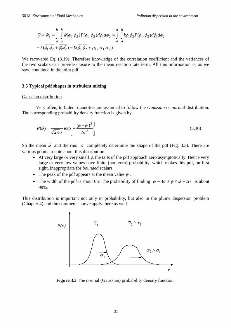
Very often, turbulent quantities are assumed to follow the Gaussian or normal distribution.
The corresponding probability density function is given by
2
2
2
)(exp
2
1)(
P (3.30)
So the mean and the rms completely determine the shape of the pdf (Fig. 3.3). There are
various points to note about this distribution:
At very large or very small , the tails of the pdf approach zero asymptotically. Hence very
large or very low values have finite (non-zero) probability, which makes this pdf, on first
sight, inappropriate for bounded scalars.
The peak of the pdf appears at the mean value .
The width of the pdf is about 6. The probability of finding 33 is about
99%.
This distribution is important not only in probability, but also in the plume dispersion problem
(Chapter 4) and the comments above apply there as well.
v
P(v)
1
2
v1
1
v2> v1
Figure 3.3 The normal (Gaussian) probability density function.

5R18: Environmental Fluid Mechanics Pollution dispersion in the environment
32
Jointly-Gaussian pdf
A usual shape for joint pdf’s in turbulence is the jointly Gaussian or joint normal pdf (Fig.
3.4):
21221
21
12
1),(
P
22
222
21
22111221
211
212 2
)())((
2
)(
)1(
1exp
(3.31)
We will encounter this equation again in Chapter 4 in the case of plume diffusion.
v
v
1
v1
2
v2
2
1
12
v
v
v1
v2
2
1
12 12
Figure 3.4 The joint normal probability density function for uncorrelated, positively and negatively
correlated variables. Equal-probability contours are shown.
Uniform distribution
If is equally probable to take any value between a and b, then P() is called the uniform
distribution and the pdf is simply equal to )/(1)( abP . In two dimensions and for uncorrelated
variables, )(
1
)(
1),(
221121
ababP
. This situation is not very common in turbulence for a
5R18: Environmental Fluid Mechanics Pollution dispersion in the environment
33
scalar or the velocity. However, the uniform distribution is extremely useful as an analytical tool
because other distributions can be related to it.
Bounded pdfs
In many situations of interest, the scalar is bounded. For example, if corresponds to a
concentration of pollutant in air, it cannot be less than zero nor higher than the maximum value it
had at the source. In this case, a=0 and b=max. The pdf should, strictly speaking, be represented by
an expression that reflects this bounded character.
Various techniques to achieve this have been proposed. One is to use a “clipped Gaussian
distribution”, where delta functions of variable strengths are used at the extrema points (a and b).
Another is to use the so-called “beta function pdf”. Both have been used in turbulent reacting flows,
but are analytically complex to represent. Qualitative shapes of pdfs for inert scalars corresponding
to a typical mixing flow are given in Fig. 3.5. For a deeper discussion, see Bilger (1980).
Pdfs of reactive scalars
Unfortunately, the chemical reaction changes the shape of the pdf in an unknown way.
Hence, no simple shape can be provided. The situation is even worse for the joint pdf of two
reactive scalars. However, there are methods by which the joint scalar pdf can be numerically
evaluated. It is evident from Eqs. (3.19) or (3.28) that knowledge of the shape of the joint pdf is
sufficient to close the turbulent reacting flow problem, and hence a lot of research emphasis has
been put in developing such methods (Pope, 2000). We will present a very simplified but still
powerful technique for estimating the statistics of random phenomena in Chapter 5.

5R18: Environmental Fluid Mechanics Pollution dispersion in the environment
34
A B
0 1
A
1
1
2
2
33
1
2
3
0 1
B1
2
3
Figure 3.5 Pdf shapes of a bounded inert scalar for a typical turbulent mixing flow.

5R18: Environmental Fluid Mechanics Pollution dispersion in the environment
35
3.6 Worked examples
Example 3.1
Show that the average of a linear function is equal to the function of the average.
Solution
Let BxAxfy )( . Then:
)()()()()()()()( xfxBAdxxxPBdxxPAdxxPBxAdxxPxfxfy
b
a
b
a
b
a
b
a
Example 3.2
Assume that the concentrations of NO and O3 measured one day are uncorrelated and obey
a joint uniform density function, with both pollutants taking values between 0 and 40 ppb. Calculate
the probability that both pollutants exceed 30 ppb.
Solution
The required probability is 16
1
0)-0)(40-(40
1 21
40
30
40
30
dd . Alternatively, we can solve
this graphically. Since both variables have the same extreme values (same sample space) and are
uncorrelated, the joint uniform distribution will look like a square (see below). The probability that
both pollutants exceed a given value is given by the area of the shaded square, which is equal to
1/4 x 1/4 = 1/16 (since the area of the whole rectangle is unity, by the normalization condition). The
same concept can by used for more relevant pdf shapes (e.g. normal distribution), but then the
calculation of the probability necessitates resort to tables that tabulate values of the integral of the
Gaussian.
NO 30
O3
40 0
30
0
40

5R18: Environmental Fluid Mechanics Pollution dispersion in the environment
36
4. Air Quality Modelling and plume dispersion
In this Chapter, we will discuss in detail some of the tools used currently in predicting the
dispersion of pollutants in the atmospheric environment. We begin from the simplest method, the
box model, and we proceed to the paradigm problem of plume dispersion. We emphasize the
practical applications and future directions of Air Quality Modelling.
4.1 Box models
Basic idea
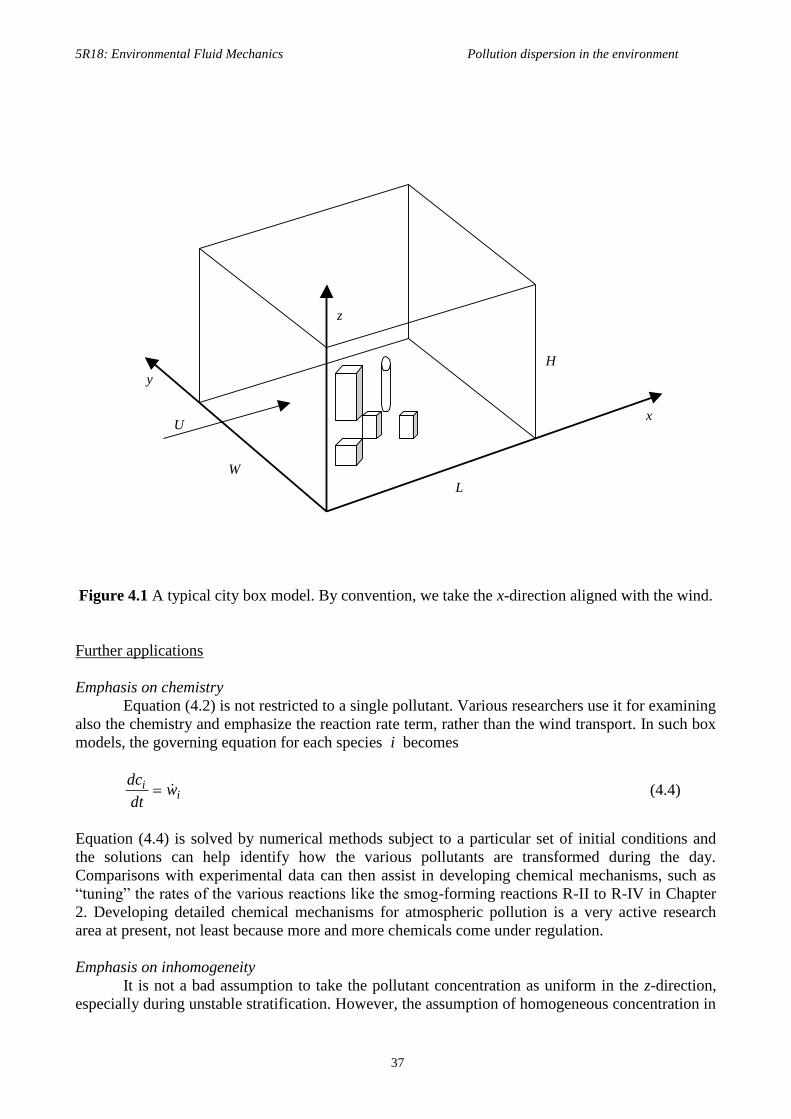
Consider Fig. 4.1, where we have enclosed a whole city in a control volume. Assume that
the air in the box is fully uniform in concentration and that there is uniform wind of velocity U
flowing along the x-direction. Assume that the box extends up to the mixing height H. Assume that
there is background pollution b (a convenient and common unit is in kg of pollutant per m3 of air)
that is being advected towards the city by the wind and that the city itself generates q kg/m2/s of
the pollutant. Then, the conservation of mass for this pollutant gives for its concentration c in the
box (in the same units as b):
cwWHLqWLUWHcUWHbdt
dcWLH (4.1)
cwH
q
L
Ucb
dt
dc )( (4.2)
The l.h.s. of Eq. (4.1) is the unsteady accumulation of the pollutant. The first term on the r.h.s. is the
amount of pollutant advected into the box by the wind; the second term is the amount advected out
of the box (note that what is being advected out has concentration c, the concentration of the well-
mixed box); the third term shows how much c per unit time is released in the city (e.g. by factories
or cars); the last denotes how much c is being generated by chemical reactions (e.g. by
transformations from other pollutants). The reaction rate cw has units kg of pollutant per unit
volume.
Very often we are interested only in the steady state, i.e. dc/dt=0. Let us also neglect
reactions, which is a good approximation if the particular pollutant reacts very slowly compared to
the residence time L/U. Then, Eq. (4.2) gives that the pollutant will be in a concentration cbm above
the city, given by
UH
qLbcbm (4.3)
This is the “standard” box model result used in Air Quality Modelling practice and hence the
subscript bm in Eq. (4.3).
Equation (4.3) involves many assumptions, the most important of which are that the
pollutant is uniformly distributed in the box, that the wind is uniform (despite the boundary layer!),
and that the emission is uniformly distributed across the area of the city. Clearly, none of these
assumptions is really justified. Nevertheless, Eq. (4.3) shows the correct scaling with H and U: low
mixing heights and low winds imply a higher concentration of pollutant. Note also that the local
city meteorology affects the pollution concentration through the wind U and the mixing height H.
Hence we expect a larger concentration of pollutant at night (small H, small U) than at day,
although this may be counterbalanced by the higher emissions during daytime (e.g. from traffic).
5R18: Environmental Fluid Mechanics Pollution dispersion in the environment
37
H
W L
x
y
z
U
Figure 4.1 A typical city box model. By convention, we take the x-direction aligned with the wind.
Further applications
Emphasis on chemistry
Equation (4.2) is not restricted to a single pollutant. Various researchers use it for examining
also the chemistry and emphasize the reaction rate term, rather than the wind transport. In such box
models, the governing equation for each species i becomes
ii w
dt
dc (4.4)
Equation (4.4) is solved by numerical methods subject to a particular set of initial conditions and
the solutions can help identify how the various pollutants are transformed during the day.
Comparisons with experimental data can then assist in developing chemical mechanisms, such as
“tuning” the rates of the various reactions like the smog-forming reactions R-II to R-IV in Chapter
2. Developing detailed chemical mechanisms for atmospheric pollution is a very active research
area at present, not least because more and more chemicals come under regulation.
Emphasis on inhomogeneity
It is not a bad assumption to take the pollutant concentration as uniform in the z-direction,
especially during unstable stratification. However, the assumption of homogeneous concentration in

5R18: Environmental Fluid Mechanics Pollution dispersion in the environment
38
the wind direction is usually much worse because often q is a function of x. This can be partly dealt
with by re-deriving Eq. (4.2) for a thin strip of thickness x and hence obtaining a differential
equation for dc/dx. (The derivation is given as an exercise in the Examples Paper. See also Example
4.2.)
Emphasis on yearly averages
Very common in Air Quality Modelling, Eq. (4.3) is used for a range of wind directions and
speeds and a range of mixing heights, so that various meteorological conditions can be examined to
find the corresponding pollutant concentrations. These are then weighted by the probability of
occurrence of these particular conditions and hence a yearly average pollutant concentration can be
calculated. Such calculations are important, e.g. for planning anti-pollution measures, for
calculating the extra environmental burden of new industrial plants, etc.
4.2 Gaussian dispersion models
Model problem
The paradigm problem concerning pollution relatively close (e.g. a few km) to a source is
the “chimney plume”. This is shown on Fig. 4.2. We are interested in: (a) the width of the plume
downwind; (b) the concentration of the pollutant across the plume and particularly on the ground;
(c) the difference between a steady emission (a “plume”) and an unsteady emission (a “puff”). To
calculate these items is very important from a practical point of view and forms the topic of this
Section. The material in this Section is based mostly on De Nevers (1995) and Csanady (1973).
x
y
z
U 0
z
Figure 4.2 A typical chimney plume, showing the definition of the quantities used in the analysis.

5R18: Environmental Fluid Mechanics Pollution dispersion in the environment
39
Turbulent diffusion of an unsteady puff
Derivation
In many cases, we are interested in the way a pollutant spreads under the action of turbulent
diffusion, when the emission of the pollutant is not continuous, but occurs only for a short time. Our
full governing equation (Eq. 3.12) is our starting point, but to demonstrate how the solution comes
about, let us assume zero mean velocities and finite and spatially-uniform turbulent diffusivity.
Then, Eq. (3.12) becomes:
wx
Kt
j
j
2
2 (4.5)
The overbar denotes the mean concentration of the pollutant and the eddy diffusivity is now
allowed to be a function of the direction. This is usually the case in atmospheric turbulence: the
velocity fluctuations are not really equal in the three directions, and hence the eddy viscosity is
strictly speaking a (diagonal) tensor. Hence the appearance of the subscript j in K in Eq. (4.5). We
have also denoted the turbulent diffusivity by the symbol K (rather than DT) to conform to the
standard notation in atmospheric pollution.
For an inert pollutant, Eq. (4.5) is identical to the unsteady heat conduction equation for an
“instantaneous source” and has a known solution. If Q kg/s of pollutant are released over a (very
short) time t at point (x0,y0,z0), the solution of Eq. (4.5) gives for the mean pollutant
concentration in one, two, and three dimensions (in kg/m, kg/m2, kg/m
3 respectively):
xxK
xx
tKt
tQx
20
2/12/1
)(
4
1exp
)()(2)(
(4.6)
yxyxK
yy
K
xx
tKKt
tQyx
20
20
2/1
)()(
4
1exp
))((4),(
(4.7)
zyxzyxK
zz
K
yy
K
xx
tKKKt
tQzyx
20
20
20
2/12/3
)()()(
4
1exp
)()(8),,(
(4.8)
where t is the time from the release. Note the “symmetry” of the terms in the exponential, but also
note that the behaviour of the maximum concentration at the centre of the cloud (i.e. at x0,y0,z0) has
a different scaling with time depending on the dimensionality of the problem.
In practical atmospheric dispersion of pollutant clouds, the wind has to be taken into
account. The situation is visualized in Fig. 4.3. The governing equation becomes (for an inert
pollutant)
2
2
2
2
2
2
zK
yK
xK
xU
tzyx
(4.9)
The solution of Eq. (4.9) is again Eq. (4.8), but now we must interpret the time t as the downwind
distance X of the centre of the pollutant cloud, divided by the wind speed U, and x,y,z as the
distances from the centre of the cloud. In Eulerian coordinates (more useful!), x should be replaced

5R18: Environmental Fluid Mechanics Pollution dispersion in the environment
40
by (x-X), with X=Ut. Usually, the coordinate system we use has an origin immediately underneath
the release point on the ground (i.e. x0=y0=0) (Fig. 4.3) and so the “standard” form of the solution of
Eq. (4.9) reads:
zyxzyxK
zz
K
y
K
Utx
tKKKt
tQzyx
20
22
2/12/3
)()(
4
1exp
)()(8),,(
(4.10)
Depending on the relative magnitude of the K’s, the cloud may take a spherical or ellipsoidal or
even a disk-like shape.
Final equation
Very often in atmospheric dispersion, we do not use the eddy diffusivities directly, but we
work with the dispersion coefficients, defined by:
xx KU
X22 , yy K
U
X22 , zz K
U
X22 (4.11)
Using the dispersion coefficients (units: m), Eq. (4.10) becomes
2
20
2
2
2
2
2/3 2
)(
22
)(exp
)2(),,,(
zyxzyx
zzyUtxtQtzyx
(4.12)
which is a “standard” Gaussian expression. The dispersion coefficients are usually functions of X
and we will present empirical data for their values in sub-section 4.3. It is important to note that Eq.
(4.12) is valid even if the eddy diffusivities K are not constant. This would be the case for short
times from the release because then the constant eddy diffusivity idea breaks down: for small cloud
widths, the pollutant is being dispersed by the action of only a small range of the turbulent eddies.
This makes the diffusivity a function of time, until the cloud becomes large relative to the
turbulence lengthscale. In atmospheric problems, this is hardly ever achieved and the dispersion
coefficients in the above equations must be provided empirically.
Equation (4.10) (or Eq. 4.12) is called the “Gaussian puff equation” and is very useful in
providing numerical estimates on the average amount of pollutant reaching a given point at a given
time after a release. Such estimates are crucial for assessing the danger after accidents, such as the
Chernobyl nuclear disaster or chemical releases. They are also used to assess the origin of the
pollutant, given a set of measurements of the pollutant concentration at a particular point and the
meteorological conditions prevailing at that time.
Cloud width
Another use of Eq. (4.12) is to find the width of the cloud. This can be defined in various
ways, since the concentration reaches zero asymptotically towards the edge of the cloud. A common
way is to use the length UXK yy /22 2 as a characteristic half-width of the Gaussian cloud
in the y-direction and similarly for the other directions. This length marks the location from the
cloud centre where the concentration falls to 1/e of the centre value.

5R18: Environmental Fluid Mechanics Pollution dispersion in the environment
41
x
y
z
U z
0
X
Figure 4.3 A typical pollution puff, showing the definition of the quantities used in the analysis.
Turbulent diffusion of a steady plume
Derivation
One way to understand the continuous emission from a chimney (Fig. 4.2) is to view it as a
series of “instantaneous puffs”. Based on the linearity of Eq. (4.9), the overall concentration
downwind would be the sum over all such puffs. Assume then that the chimney continuously
releases Q kg/s of pollutant and we use t=x/U. We are interested in the pollutant concentration at a
particular point (x,y,z) at time t. Equation (4.12) can be integrated over time, to give the mean
concentration due to a continuous source:
02
20
2
2
2
2
2/3'
1
2
)(
22
)'(exp
)2(),,( dt
zzyUtxQzyx
zyxzyx
(4.13)
It is important to remember that we are now dealing with diffusion at early times, i.e. we are
interested in the region close (e.g. of the order of 10 to 104 m) to the plume source. There, the
width of the plume is clearly not much greater than the turbulence lengthscale, which is one of the
conditions for validity of the constant eddy diffusivity. For short distances from the source, it turns
out that the dispersion coefficients are proportional to time:
tux , tvy , twz (4.14)

5R18: Environmental Fluid Mechanics Pollution dispersion in the environment
42
where u , v , w are the r.m.s. turbulent velocities in the three directions, assumed constant.
Equation (4.13) can then be integrated (after a very long and difficult procedure) to give:
ru
Uxerfc
ru
xU
ru
Ux
u
U
rwv
uQzyx
2
1
2exp
21
2exp
)2(),,(
22
22
2
2
22/3
(4.15)
with 2
02
22
2
222 )( zz
w
uy
v
uxr
. Usually, the plume is slender, which implies that r x , and
usually 1)1.0(/ oUu . Both these assumptions are used to simplify Eq. (4.15) into:
2
20
2
2
22exp
1
2),,(
zyzy
zzy
U
Qzyx
(4.16)
This is our final result for the plume diffusion problem and is one of the most important
equations in this set of Lectures. It is often called the “Gaussian plume equation”. The x-
dependence comes indirectly through the dependence of the disperion coefficients on x, while the
dependence on y and z comes directly from the exponential.
Diffusion from a point source
The slender plume approximation is equivalent to neglecting the axial diffusion because,
compared to the advection, it causes little spreading. Equation (4.16) is also the solution of the
general governing equation for a statistically-steady inert scalar being injected at a rate Q at point
(0,0,z0), with x-wise diffusion neglected:
2
2
2
2
zK
yK
xU zy
This problem is also known as “diffusion from a point source” and its solution is Eq. (4.16), with
dx
dUK
yy
2
2
and
dx
dUK z
z
2
2
. Experimentally, the K’s are found indirectly by measuring the
concentration across the plume, applying Eq. (4.16) to the measured profiles, and hence evaluating
. This has proven to be a very useful tool to understand atmospheric turbulence and dispersion.
The eddy diffusivities so found are called “apparent eddy diffusivities”.
Short and long time diffusion
For short distances, we have that UxvtvK y /22 , UxwtwKz /22 , while for long
distances from the source we obtain yyLy LvTvK ,2 , zzLz LwTwK ,
2 , where TL,y is the
Lagrangian autocorrelation time in the y-direction, Ly is an equivalent lengthscale, and similarly for
the z-direction. Because in general wv and zLyL TT ,, , in general zy KK . Equation (4.12) for
the cloud and Eq. (4.16) for the plume turn out to be valid for both short and long time mixing, with
the difference that the dispersion coefficients are a different function of x in the two cases. From
Eqs. (4.11) and (4.14), the width of the plume increases linearly with x for short times, while it
increases as x1/2
for long times.

5R18: Environmental Fluid Mechanics Pollution dispersion in the environment
43
The difference between short and long-time diffusion is important for the theoretical study
of turbulent mixing. If the release occurs at a length of the order of the Kolmogorov scale, then
there is an additional, “very early” time regime, where the plume grows by the action of molecular
motions, and there too, it grows as x1/2
, but with a molecular, rather than a turbulent, diffusivity
appearing in the proportionality constant. This is irrelevant to atmospheric pollutant problems, as
the emission lengthscale – the stack diameter – is much larger than the Kolmogorov scale.
The Gaussian
Equation (4.16) is identical to a joint Gaussian expression in Section 3.5, Eq. (3.31), with
12=0. This is no coincidence: in order to derive Eq. (4.16) we have implicitly assumed that the
turbulent motions in the two directions are uncorrelated. This would not be so if there were shear in
the air flow, which would give rise to finite Reynolds stresses. The presence of Reynolds stresses
would make a cross-section of the plume look skewed (c.f. Fig. 3.4) and Eq. (4.16) would need
correction. This is often done for predicting dispersion in the atmospheric boundary layer, but is
beyond the purposes of this course.
Self-similar solutions
There is an alternative way to derive Eq. (4.16). This is based on the concept of self-
similarity, which is presented (for one-dimensional spreading) in the Appendix.
Measurements of the dispersion coefficients
In order to use Eq. (4.16) in practical applications, we need to know the dispersion
coefficients y and z. These will be functions of downwind distance x and will also be unequal,
since the characteristic turbulence velocities are expected to be different in the horizontal and
vertical directions. Finally, we expect them to depend on atmospheric conditions: for stable
conditions, the r.m.s. velocities are very low and hence the dispersion coefficients small; for
unstable conditions, the turbulence is vigorous and we expect much larger dispersion coefficients.
Measurements over a range of stability conditions give the results plotted in Fig. 4.4. Due to the
complexity of atmospheric turbulence, the dispersion coefficients increase with x at a rate between
1 and 1/2, with the vertical dispersion coefficient increasing at a variable rate with x and the
horizontal at about 0.9. The various curves correspond to various stability classifications, described
in Table 4.1. From this Table and Fig. 4.4, the ’s can be estimated at a given downwind distance
and hence Eq. (4.16) can be applied to give the mean pollutant.
Table 4.1 Stability categories of Pasquill (adapted from De Nevers, 1995). A to F refer
progressively from the very unstable to the very stable conditions, with D the neutral.
Wind speed
at 10 m high
(m/s)
Day Night
Solar intensity
Strong Moderate Slight Overcast Clear
0-2 A A-B B - -
2-3 A-B B C E F
3-5 B B-C C D E
5-6 C C-D D D D
> 6 C D D D D

5R18: Environmental Fluid Mechanics Pollution dispersion in the environment
44
(a)
Figure 4.4 Horizontal (a) and vertical (b) dispersion coefficients as a function of downwind
distance from the source for the “standard” stability conditions of Table 4.1 (De Nevers, 1995,
quoting Turner).

5R18: Environmental Fluid Mechanics Pollution dispersion in the environment
45
(b)
Figure 4.4 Cont’d.
Ground concentrations
One of the most important applications of the Gaussian plume equation is to calculate the
pollutant concentration on the ground some distance downstream from the source. If the ground
does not absorb any pollutant, then it “reflects” the pollutant reaching it. This is modelled by putting
a “mirror image” source at z = z0, and then calculating at any point the combined effect of the two
sources. Therefore, the Gaussian plume equation is modified to account for the ground effect as:

5R18: Environmental Fluid Mechanics Pollution dispersion in the environment
46
2
20
2
2
2
20
2
2
22exp
22exp
1
2),,(
zyzyzy
zzyzzy
U
Qzyx
(4.17)
At z=0 (i.e. on the ground), the pollutant concentration is
2
20
2
2
22exp
1)0,,(
zyzy
zy
U
Qyx
(4.18)
and along the x-direction (the axis of the plume) on the ground we get
2
20
2exp
1)0,0,(
zzy
z
U
Qx
(4.19)
Equation (4.19) is very useful for predicting the amount of pollutant (kg/m3) reaching a receptor
downwind from a pollution source emitting Q kg/s. It is used for assessing the environmental
effects of various industrial plants etc. Note that the calculation depends crucially on the magnitude
of the dispersion coefficients, and hence estimates such as those offered by Table 4.1 and Fig. 4.4
are very important for practical Air Quality Modelling.
When the ground is absorbing the pollutant, the image source idea can still be used, but now
the image source must have a negative strength, i.e. the second exponential term in Eq. (4.17)
should appear with a minus sign.
One-dimensional spreading
Diffusion in the vertical direction can occur only up to the mixing height H (Section 2.4). It
happens often that the mixing height is low and then it does not take very long for the pollutant to
become virtually homogeneously mixed in the vertical direction, but still diffusing in the horizontal
direction. The horizontal concentration distribution is such cases will be given by:
2
2
2exp
2
1),(
yy
y
UH
Qyx
(4.20)
which is useful and quite easy to remember. This equation is identical to the standard Gaussian, Eq.
(3.30). From Eq. (4.20), we observe that the maximum concentration occurs at y=0 and is equal to
)2/( yUHQ .
Another problem where we have one-dimensional spreading is in “diffusion from a line
source”. A motorway, for example, can be taken as a line source on the ground (z0=0), emitting
Q/L kg of pollutant per unit time and unit length. We usually take the source aligned with the y-axis
and the wind with the x-axis. The pollution will be advected downwind and diffusion will occur in
the vertical direction. The concentration profile in the vertical direction will be given by:
2
2
2exp
2
12),(
zz
z
UL
Qzx
(4.21)

5R18: Environmental Fluid Mechanics Pollution dispersion in the environment
47
with the x-dependence coming from the x-dependence of the dispersion coefficient (e.g. Fig. 4.4).
Note that we still need an image line source, but now both sources coincide at z0=0 (hence the 2 in
the numerator). Equation (4.20) for the plume with vertical homogeneity is equivalent to diffusion
from a vertical line source of strength Q/H, of course without any reflection since no boundaries
exist normal to the y-direction.
Plume rise
Very often, the exhaust gases from chimneys are hotter than the environment or they have
substantial momentum. This makes them rise and hence the release height z0 that should be used in
the Gaussian puff and plume equations does not correspond truly to the stack height hs. Instead, it
corresponds to the stack height plus the “plume rise” distance hpr, which is the approximate height
above the stack before the plume turns 90 to follow the wind. To predict buoyant plume rise
theoretically would involve a combined examination of momentum and buoyancy in the curved
plume and is a little involved. An empirical relationship used sometimes by engineers designing
stacks is:
s
atmsspr
T
TTPD
U
DVh 68.25.1 (4.22)
with hpr the plume rise (m); Vs the stack exit velocity (m/s); D the stack diameter (m); P the pressure
of the atmosphere (bar); and Ts and Tatm the temperatures of the stack gas and the atmosphere
respectively (K).
4.3 Effects of local meteorology
Effect of inversions
We mentioned in Section 4.2 that the case of one-dimensional diffusion in the horizontal
direction approximately corresponds to the case where the plume is perfectly mixed in the vertical
direction. If the mixing height is higher than the source height, i.e. if H > (hs+hpr), then there is
every possibility that the plume will hit the inversion lid from below, from where it will be reflected
downward etc. This situation is shown in Fig. 4.5, which also demonstrates how the image source
idea can be used to account for the mixing height. It is clear that the vertical direction will
eventually become quite homogeneous.

5R18: Environmental Fluid Mechanics Pollution dispersion in the environment
48
x
z
U
z 0 H
Image source
Real source
Figure 4.5 Effect of inversion lids on diffusion from a source below the inversion.
Equation (4.20) applies in this case for distances far enough from the source. Since vertical
diffusion is eliminated, the ground concentration decays as x1
(since, approximately, y ~ x1; Fig.
4.4), in contrast to a faster decay if the diffusion were two-dimensional (in the 2-D case, from Eq.
4.19 the maximum ground concentration decays by an additional z1
). Therefore, low mixing
heights will result in higher ground concentrations.
Inversions assist in “trapping” pollution above a city, which can be thought as composed of
a very large number of point sources. Cities with serious smog problems like Los Angeles, Athens,
Istanbul and others, are located in sunny regions, bounded by mountains, and are close to the sea. In
addition to more intense photochemistry, these conditions are favourable for the creation of
inversion lids and hence such cities encounter high levels of pollution often.
Plume shapes
Depending on the conditions close to the plume source, the plume may acquire shapes very
different from the “regular” diffusion shape defined by Eqs. (4.16) (without ground effect) and
(4.17) (with ground effect). Various plume shapes and associated phenomena are described next
and shown in Fig. 4.6.
Fumigation
If a plume is emitted into a very stable atmosphere (e.g. during a clear night), the plume
travels downwind with very little dispersion. After dawn, as the sun heats the ground, an unstable
layer is formed and the mixing height associated with the edge of this layer travels upwards as time

5R18: Environmental Fluid Mechanics Pollution dispersion in the environment
49
progresses. When this turbulent layer hits the plume, it causes very quick transport of the pollutant
to the ground. This episode is called fumigation and it can result in very high ground
concentrations, but for relatively short times.
Lofting
If either due to a very high stack or due to very high buoyant plume rise the plume source is
effectively above the inversion, then the plume is dispersing upwards, but not downwards. The
inversion acts like a solid boundary. This situation protects the ground receptor from high pollutant
levels.
Fanning
If the plume source is within an inversion layer, it spreads horizontally but not vertically.
This is called fanning and in such situations, the plume can travel long distances with little dilution.
Trapped plume
If the plume is below the inversion, it cannot penetrate it and the pollutant is not dispersing
upwards. This causes higher ground concentrations than if the inversion were not there and is often
the reason for high pollution levels in cities.
Downwash
Often it may happen that the stack sheds vortices or that the stack is in the wake of a large
building. In both cases large eddies may trap the plume and push it towards the ground. These
situations are called downwash or flagging and downdraught respectively. A rule of thumb by
engineers is to use a stack height at least 2.5 times the height of the nearest building. Good
aerodynamic design of the stack can help in reducing downwash. The same effect appears when the
source is situated near a mountain, where the katabatic winds may not allow normal, Gaussian
dispersion, but cause a bulk movement of the plume towards the ground. Katabatic winds also
favour the creation of inversion lids by bringing cooler air close to the ground.
Looping
In very unstable situations, the eddies causing plume dispersion may be much larger than the
plume width. This results in a “solid-body” motion of the plume, also called the “meandering
plume”. See Section 5.3 for more discussion on this.
Thermalling
If the plume is very buoyant, it may break up in distinct parcels, as the plume itself is
initiating thermals.

5R18: Environmental Fluid Mechanics Pollution dispersion in the environment
50
Fumigation
Lofting
Trapped plume
Downwash
Looping
Thermalling
Fanning
Figure 4.6 Some common plume shapes.

5R18: Environmental Fluid Mechanics Pollution dispersion in the environment
51
4.4 Practical Air Quality Modelling
In Section 4.2, we presented the “Box Model”, which is a very useful tool for estimating the
pollution above a city. Such box models are used in scales of a few km. If one is interested in finer
scales (e.g. a few hundred metres), and this may be imperative for accurate calculations of dosage,
e.g. from a new industrial plant or a planned motorway, then we need to consider the dispersion
very close to the source. For uniform wind conditions and well-defined sources, the Gaussian plume
theory is approximately correct for up to a few tens of km, but eventually our assumption of
constant wind will becomes invalid. For synoptic scales, i.e. longer than 200 km, we need to couple
our pollution dispersion models with proper meteorological (i.e. weather prediction) codes.
Eulerian codes
In current practice, researchers solve Eq. (3.12), with proper attention to the chemistry and
to phenomena such as deposition, aerosol formation, turbulence inhomogeneity and anisotropy,
stratification etc. They do so after discretizing the p.d.e. on a grid of resolution applicable to the
problem at hand. Because of this, they are also called “grid models”. The numerical techniques used
are a very active research area. It is imperative that such codes can predict the evolution of
pollutants from accidents or from a particular set of meteorological conditions in a short period of
time (e.g. a few hours or days of CPU time), in order to be in a position to issue warnings about
pollution episodes.
A serious scientific problem with Eq. (3.12) is how to model the chemical source term. This
is still an unclosed issue and the current generation of codes use simply a mean reaction rate
calculated from the mean species concentrations. We have seen in Section 3.2 and 3.3 that doing so
is wrong, as it involves neglect of the species concentration fluctuations. In some cases, this is
justified, as we will see in Ch. 5, but in many others, it is not.
The representation of the mean source term and of the turbulent diffusivity is the weakest
points of practical AQM codes. In addition, the chemistry is not as well known as required to make
very accurate predictions. AQM practitioners are happy to live with greater uncertainties than in
other engineering fields.
Lagrangian codes
A different approach to track the dispersion and chemical evolution of pollutants is the so-
called Lagrangian approach. Here, a large number of “fluid particles” is tracked in the synoptic
scale weather motions and the chemistry of each of these particles is calculated with Eq. (4.4). Such
calculations have shown, for example, the amount of radioactive material reaching Western Europe
following the Chernobyl nuclear accident in 1986. They are also called “trajectory models”.
This approach has the advantage of having relatively lost cost, but the accuracy of some of
the assumptions used in early versions of this method is not very good, especially the modelling of
the turbulent random walk experienced by the fluid as they disperse in the air. Despite this
reservation, the idea of modelling the fluid as individual particles and then tracking the changes in
each of these is a very useful one and the improvement of the accuracy of such models is a topic of
research now.
The US Environmental Protection Agency Web Site
A series of links to the codes used in practical AQM can be found at the US EPA Web site:
http://www.epa.gov/scram001/tt22.htm#rec

5R18: Environmental Fluid Mechanics Pollution dispersion in the environment
52
4.5 Worked examples
Example 4.1
A box model for a city has W=5 km, L=15 km, the mixing height is H=1 km, and the wind is
blowing along the long dimension of the city with U=5 m/s. The background concentration of CO
coming into the city is b=5x10⁹
kg/m3, and the emission rate is q=4x10
9 kg/sm
2. Find the
concentration of CO above the city.
Solution
This is a straightforward application of Eq. (4.3) and is intended to give an idea on the order
of magnitude of the quantities used in conjunction with city box models. Putting numbers gives
cbm=25x109
kg/m3. Note that the result is independent of the width of the city.
Example 4.2
The worst assumption in the standard box model is that the concentration is uniformly
distributed along the wind direction. By doing a mass balance on infinitesimally thin strips normal
to the wind, the following o.d.e. can be derived for c(x) (the derivation is given as an exercise in the
Examples Paper): wHxqdxUdc /)(/ . Assume now that the pollutant undergoes photolysis, so
that it is being destructed at a rate kcw . Find c(x) if q is constant and if no pollutant enters the
city.
Solution
Since no pollutant enters the city, c(0)=0. Then, solving the o.d.e. gives:
dx
cU
k
UH
q
dcc
U
k
UH
q
dx
dcw
H
xq
dx
dcU
)(
)exp(1)( x
U
k
kH
qxc
Therefore, the concentration of c will become equal to q/kH at x long compared to U/k. If
photolysis were absent (k=0), integrating the o.d.e. would give that c=qx/UH, i.e. the pollutant is
continuously increasing with downwind distance and we recover Eq. (4.3) for x=L. Photolysis
reactions and other removal mechanisms (e.g. deposition to ground by rain) are important in
controlling the levels of atmospheric pollution.
Example 4.3
An accident in a chemical factory releases 1000 kg of SO2 from a chimney. The pollutant
cloud is assumed to rise vertically upwards very quickly and then it is transported horizontally by
the wind blowing with 5 m/s. The three turbulent diffusivities are estimated as 100 m2/s. Estimate
the width of the cloud 5 km downstream and the pollutant concentration at the centre of the cloud.
Solution
This is a straightforward application of Eq. (4.10). The concentration at the centre will be:

5R18: Environmental Fluid Mechanics Pollution dispersion in the environment
53
2/12/30)()/(8
),0,(
zyx KKKUX
qzX
, with q=1000 kg, X=5 km, Kx=Ky=Kz=100 m
2/s, and
U=5 m/s. The width of the cloud is estimated as UKX /4 (since we want the total width). Putting
numbers, we get that 2SO 7.1x10⁷
kg/m3 and the cloud width is 1265 m.
Example 4.4
The effluent stream in a refinery is at 1 bar and 300 K and flows at 10 m/s from a chimney
of diameter of 200 mm. The exhaust gases contain 100 ppm (by mass) of VOC’s and the chimney is
20 m high. Neglecting any plume rise, find the ground concentration 10 km downwind the refinery
for the following conditions: (i) wind of 2.5 m/s at night on a clear night; (ii) wind of 8 m/s on a
sunny day with strong sunlight. Calculate the horizontal width of the plume at this point. If the
atmospheric temperature is 280K, is the assumption of negligible plume rise valid?
Solution
This is a straightforward application of Eq. (4.19). The mass flow rate of the pollutant at the
source is Q=(100x106
) x (/287/300) x (0.2
2/4) x 10 kg/s = 3.65 x10
5 kg/s. The dispersion
coefficients for the given conditions at x=10 km are given from Table 4.1 and Fig. 4.4 as: (i)
category F, so y=280 m and z=50 m; (ii) Category C, so y=800 m and z=530 m. Therefore,
from Eq. (4.19), we obtain that the ground concentration is (i) 3.1x10¹⁰
kg/m3 and (ii) 3.4x10
12
kg/m3.
The horizontal width of the plume at that location can be defined as twice the y-coordinate
where the value of the pollutant is 1/e of its value along the centre. This occurs at 22 2 yy , which
gives the overall width of the plume as 792 m for case (i) and 2263 m for case (ii). To calculate the
plume rise, we use the empirical formula Eq. (4.22) which gives that hpr=1.34 m for case (i) and
0.42 m for case (ii). Hence, we were justified to neglect it, more so for the strong wind case (ii).
This example demonstrates the major alterations to the plume dispersion process expected
from a switch from stable to unstable stratification conditions.
Example 4.5
For the plume of Example 4.4, find the point immediately below the axis of the plume on
the ground (i.e. y=0, z=0) that has the highest pollutant concentration. Assume that my Ax and
nz Bx .
Solution
Differentiating Eq. (4.19) with respect to x and using the given variation of the dispersion
coefficients with x, we get that 0/)0,0,( dxxd when n
mz
z22
1
2 2
20
. It is a reasonable
approximation to assume that m/n is not substantially different from unity. Hence, the maximum
will occur when 2/0zz . Putting numbers, the maximum concentration will occur when z is
14.1 m. So reading from Fig. 4.4, for case (i), this will occur at a downwind distance of 1.5 km,
while for case (ii), the maximum ground concentration will be at about 0.25 km. Note the very
different behaviours between the two atmospheres, which shows the different possibilities between
pollution dispersion during day and night at the same geographic location.

5R18: Environmental Fluid Mechanics Pollution dispersion in the environment
54
Appendix: An alternative derivation of the Gaussian plume equation
For simplicity of presentation, we will consider only one-dimensional spreading. Assume
that Q kg/s are emitted over a line of length H parallel to the y-axis. There are no solid boundaries.
The governing equation for the mean concentration then becomes
2
2
zK
xU
(A4.1)
which is identical to the unsteady heat equation if we recognize that t=x/U. Our initial and boundary
conditions will determine the solution. Many solutions of Eq. (A4.1) are given in advanced heat
transfer books. An alternative way to show the rationale behind the solution we used (Eq. 4.20), is
to seek self-similar solutions. By “self-similar” we mean solutions that depend on one independent
variable only, which is a combination of the two dependent variables t and z. Most slender
turbulent flows are self-similar for the velocity and the scalar fields.
Let us say that we seek a function f(), such that
)(0 f (A4.2)
/z (A4.3)
with 0 and being a function of x only. The quantity 0 is a characteristic scale of the
concentration, while is a characteristic width of the plume, both as yet undetermined. We will use
the following transformation rules:
x
f
x
f
1
z
and from Eq. (A4.3),
xx
Using the above and substituting Eqs. (A4.2) and (A4.3) in (A4.1) gives:
2
2
2000
d
fdK
d
df
dx
dUf
dx
dU
00
0
2
2
2
f
dx
d
K
U
d
df
dx
d
K
U
d
fd
(A4.4)
If we want self-similar solutions, the terms in brackets in Eq. (A4.4) must be independent of x, i.e.
constants. Let us consider the term dx
d
K
U first. Without loss of generality, we could say that this
constant is unity (if it were anything else, could be altered so that it is). This results in:

5R18: Environmental Fluid Mechanics Pollution dispersion in the environment
55
dx
dUK
dx
d
K
U 2
21
(A4.5)
which is discussed in Section 4.3. Before proceeding, we can bring in the model for the eddy
diffusivity to discover how the plume grows with x. For long times, K is constant and Eq. (A4.5)
gives that U
xK22 , i.e. we recovered Eq. (4.11). For short times, the diffusivity is proportional
to u and the characteristic length of eddies inside the plume. This is , i.e. the width of the plume
itself, since the plume cannot be mixed by eddies greater than its size. So for short times, uK ,
which gives xU
u , i.e. we recovered Eq. (4.14). We also determined how the width of the plume
grows with x: for long times, 2/1~ x , while for short times x~ .
The second requirement for self-similar solutions is that the term dx
d
K
U 0
0
2
be independent
of x. We can relate dxd /0 to dxd / by examining the overall conservation of mass of our
(inert) pollutant. Integrating across any section of the plume gives
UHQdfUHQdz /)(/ 0
(A4.6)
Denote the integral above by I. Since it is a function of only, it is independent of x. Therefore,
0 is a constant, which gives that dx
d
dx
d
11 0
0
. Hence, 1
20
0
2
dx
d
K
U
dx
d
K
U
.
Therefore, Eq. (A4.4) becomes
02
2
fd
df
d
fd
(A4.7)
with boundary conditions
1)0( f , 0)0( f (A4.8)
and the solution should obey 0)( f . It is very easy to confirm that a function satisfying all
the above is
)2/exp()( 2 f (A4.9)
(This can also be derived by solving Eq. A4.7 directly). From Eq. (A4.6), we also found that 1
0 ~ , i.e. the characteristic scale of the pollutant concentration decreases as 2/1x for long
times and as 1x for short times.
The problem is almost solved now. The mean concentration is given by

5R18: Environmental Fluid Mechanics Pollution dispersion in the environment
56
)(/1
fU
HQ
I (A4.10)
Using Eq. (A4.9) and the fact that 2/12/2
deI , Eq. (A4.10) gives the final result for
the concentration:
)2
exp(2
/2
2
z
U
HQ (A4.10)
This is identical to Eq. (4.20) for one-dimensional spreading in the z-direction (without ground
effect).
We have shown here how the concept of self-similarity and the overall conservation of
pollutant mass gave us the scaling of characteristic width and centerline concentration with
downwind distance. The approach can be extended to more dimensions. For example, for two
dimensional spreading, put )()(0 gf with zz / and yy / . Repeating the
procedure to seek self-similar solutions will result in Eq. (4.16).

5R18: Environmental Fluid Mechanics Pollution dispersion in the environment
57
5. Turbulent reacting flows and stochastic simulations
5.1 Fast and slow chemistry
Turbulence time and length scales
The turbulence has a wide range of scales. If the rms velocity fluctuation is u and the large
eddy length scale Lturb, the large eddy turnover time, Tturb, is given by
u
LT turb
turb
(5.1)
and the eddies at the Kolmogorov level have a time and length scale of
2/1
Re
tturbK TT (5.2)
4/3
Re
tturbK L (5.3)
where
/
Re turbt
Lu (5.4)
is the Reynolds number of the turbulence. For a typical location low in the atmospheric boundary
layer, we may have that u= 1 m/s, Lturb = 100 m, and for air =1.5x10⁵
m2/s. These values give
Tturb = 100 s, Ret = 6.7x10⁶, and hence TK = 0.04 s and K = 0.8 mm. So there is a very wide range
of time and length scales in typical flows in the environment.
Chemical timescales – the Damköhler number
From the presentation of chemistry in Chapter 2, it is evident that the rate of the reaction is
determined by the amount of reactant and by the reaction rate constant k. The governing equation
for a scalar (Eq. 3.9) has terms due to the fluid mechanics (advection, turbulent diffusion, molecular
diffusion) and due to the chemistry. Therefore the net rate of change of the scalar will depend on
both phenomena. Now, added to this that the various terms in Eq. (3.9) have different scaling even
without chemistry (large-eddy scaling for the mean and turbulent transport, small-eddy scaling for
the molecular diffusion), we see that the relative effect of the turbulence on the reaction will depend
on the ratio of turbulent to chemical timescales, called the Damköhler number. We usually define
two such ratios, one using the large-eddy timescale and another using Kolmogorov timescale:
2/1
121 Re ,
tchem
K
chem
turb DaT
TDa
T
TDa (5.5)
We do this because the chemical reaction occurs at the small scales, where the reactants mix at a
molecular lever, but we are also interested to know how the reactants get together in the first place,
and this is determined by the large scales. These complications are typical of turbulent flows. It is
not just a coincidence that turbulent reacting flows are considered one of the most difficult
problems in the whole of turbulence and fluid mechanics fields!

5R18: Environmental Fluid Mechanics Pollution dispersion in the environment
58
A way to define the chemistry timescale is illustrated by the following example. Take the
reaction NO + O3 NO2 + O2. The consumption rate of [NO] from this reaction is
d[NO]/dt = k[NO][O3]. Treating [O3] to be constant, we obtain d[NO]/dt = A [NO], which gives
an exponential decay with timescale defined as 1/A. Typical concentrations of NO and O3 in a
typical early morning are 3x10⁹
and 1.5x10⁹
kmol/m3 respectively and the rate constant is
k=1x10 m
3/kmol/s. Hence, for this reaction and for these concentrations, Tchem=66.7 s. This is a fast
reaction for atmospheric chemistry; others are many orders of magnitude slower. The definition of
chemistry timescales becomes more complicated if there are many elementary reactions that
consume or produce a particular species, as is almost always the case. This makes matters very
difficult, as far as theoretical predictions go.
Simplifications
Fast chemistry (Da2 1):
If the chemistry is considered to be very fast compared to all fluid mechanics scales, then
the rate of chemical reaction follows the rate at which reactants are being mixed. This is the basis of
many models, such as the “eddy break up”, the “mixed is burned” and the “eddy dissipation
concept” (Peters, 2000). All these have been used extensively in the combustion literature, where
indeed the chemistry is usually fast compared to mixing times, e.g. inside engines.
The situation is less clear concerning environmental flows. There, the large eddy time scales
are longer than in engines, but the Ret is higher, and hence the Kolmogorov time scale may not be
very different. The chemistry, on the other hand, is much slower in the atmosphere than in a flame.
This makes the fast chemistry limit invalid for atmospheric pollutants. Hence, the well-proven
techniques that are embodied in commercial CFD codes, usually tuned to combustion or other
chemical engineering problems, may not be always applicable to environmental reacting flows.
Slow chemistry (Da1 1):
At the other extreme, if the mixing times are much faster than the chemistry, we may
consider that the reactants are well-mixed, i.e. that the pollutants are uniformly distributed in space,
at least over a scale comparable to Lturb. This means that the degree of scalar fluctuation is small,
which enables us to neglect the correlation 21 . This then allows the straightforward application
of Eq. (3.19) without any need to provide closure for the turbulence effects on the reaction, which is
calculated simply using the mean concentrations (an assumption sometimes called “laminar
chemistry”).
This assumption is very often introduced in air quality models that are currently used for
monitoring and certification purposes. However, as these models progressively look into finer and
finer length and time scales (e.g. the NO emitted from cars in street canyons), the assumption of
well-mixed reactants becomes invalid. See Example 5.2 for more discussion on this.
Intermediate (Da2 1 Da1):
This is the most difficult, and the most relevant, situation, which is currently under intensive
research. No simple theory exists for this regime. One very useful and insightful technique is to
calculate the joint pdf of the scalars by numerical means, and this is introduced next.

5R18: Environmental Fluid Mechanics Pollution dispersion in the environment
59
5.2 Monte Carlo simulations
Fundamentals of Monte Carlo techniques
In Monte Carlo techniques, a large number of events are sampled from the possible sample
space and their evolution is tracked. Averages formed over many such “trajectories” give the
behaviour, in a statistical sense, of the whole system. Other, perhaps more accurate, names for this
technique include “stochastic modelling” or “stochastic simulation”. Monte Carlo techniques are
used for an immense variety of topics (e.g. statistical mechanics, molecular dynamics, chemistry,
turbulence, stock market risk analysis). The following examples aim to clarify the technique.
Example 1 of Monte Carlo simulation
Assume we have a die. Each time we roll it, we note the result (1 to 6) which we call x.
Then, we use this number to initiate the following sequence of events: (i) calculate
y(x) = (x/6)2 + sin(x/6) + x exp(x/6) ; (ii) if the result is less than 0.5, it is “YES” ; (iii) if the result
is greater than 0.5, it is “NO”. We want to calculate the probability of “YES”.
Clearly, an analytical approach is extremely difficult (but not impossible for this particular
example). The Monte Carlo approach is the following: (i) sample N random numbers from a
uniform distribution between 1 and 6; (ii) calculate y(x) for each of these N samples; (iii) for each
of the resulting y(x), determine if it gives “YES” or “NO”; (iv) count the number NYES of events
that were “YES”. The probability of getting “YES” is then simply NYES/N.
All that is needed is a computer and a random number generator (and there are plenty of
library codes in Fortran, C, or in Matlab for that).
Example 2 of Monte Carlo simulation
Assume you have £100.00 that you want to invest in 10 different stock market companies,
S1, S2, …, S10, each of which today costs A=£1.00. History suggests that the probability of S1
rising tomorrow by a fraction f1 (i.e. the value tomorrow is equal to (1+ f1)A) is given by a normal
distribution with mean 1=0.01 and rms 1=0.1. So, on average, the price of S1 tomorrow will be
£1.01, but it could be anywhere between (1.013·0.1) and (1.01+3·0.1) (to within 99%). Similar
historical data are assumed to apply to all our equities. There could also be various restrictions, for
example: if it happens that S1 becomes greater than £1.50, then S3 will fall by 10%, etc. We want to
calculate the spread in the possible worth of our investment portfolio after one month.
A Monte Carlo simulation would be to simulate a very large number of possible “scenaria”
and then evaluate the worth of the portfolio at the end of the month. The steps would be: (i) pick
randomly a value for each fi (i.e. for each stock), each according to its own distribution (assumed
known from historical data). Hence you get the new price of each stock Si. (ii) Enforce the various
restrictions (e.g. change the Si’s accordingly). (iii) Continue for the next day. After doing the
simulation for 30 days, you get the value of your investment for this particular realization. (iv)
Repeat steps (i) to (iii) for N (some thousands) of these scenaria.
At the end of the simulation, we have N possibilities, each with a different total worth of
our investment. These define the pdf of our investment value, which helps answer questions like
“what is the probability that we will lose 10% of our money” or “what is the probability that we will
gain 20%” etc.
Warning: this is a hypothetical example: DON’T TRY IT – no responsibility is borne by
the lecturer if you lose your money!

5R18: Environmental Fluid Mechanics Pollution dispersion in the environment
60
Monte Carlo simulation in turbulent reacting flows
These ideas are used to great advantage in turbulent reacting flows. The reason is that since
the chemistry is non-linear, the effect of the scalar fluctuations is not analytically tractable (i.e.
correlations develop, Eq. 3.19) and so keeping track of various “scenaria” of scalar values and
averaging over all of them, allows us to estimate the evolution, in the mean, of our system.
Assume we have a domain with homogeneous isotropic turbulence with K scalars that
participate in chemical reactions. For this spatially uniform system, the governing equation for the
mean scalar becomes:
ii w
t
(5.6)
(we need not specify in more detail the reaction rate at this stage). The mean convection and
diffusion terms disappeared due to spatial uniformity. At time t=0, each scalar i has concentration
i that is distributed according to a probability density function, say a Gaussian with mean i and
rms i and there are no correlations between the species (i.e. 0ji ). We want to calculate the
subsequent evolution of the system. Clearly, we need a model for iw , but no such model is
available and hence the direct solution of Eq. (5.6) is impossible.
Consider, however, the following surrogate to the real system: let the fluid be composed of a
large number of individual “fluid particles”. Each of these fluid particles has a random composition
such that when we average over all particles, we get the right mean and rms of the fluid
composition (i.e. the known, initial i and i). The basic steps in a Monte Carlo simulation are the
following:
(i) For each particle, pick a random composition from a Gaussian with mean i and rms i
(the index i refers to the i-th species).
(ii) Calculate the reaction rates iw for this fluid particle for all scalars i.
(iii) Solve iturb
iii wTt
(5.7)
for each scalar and for each particle from t=t0 until time t=t0+t. Equation (5.7) is a
modeled instantaneous equation for the conservation of the scalar i inside the fluid
particle (i.e. the corresponding Eq. 3.8 for the fluid particle). The first term in the r.h.s. is
a modeled turbulent diffusion term, while the second term is the chemical reaction.
(iv) We now have the new composition for each of the particles. Evaluate the new mean i
(i.e. perform an average over all particles) for all scalars.
(v) Repeat steps (ii) to (iv) until we reach the end of the time domain we are interested in.
This sequence of steps is a very simplified version of the proper Monte Carlo approach to turbulent
reacting flows, but it may serve to illustrate the basic concept. In essence, we do not look at the
fluid as a whole, but as composed of individual stochastic fluid elements. Each of these, undergoes
mixing with its neighbours (the term turbii T/ in Eq. 5.7) and chemical reactions in itself

5R18: Environmental Fluid Mechanics Pollution dispersion in the environment
61
(the term iw ). Hence, by looking at a large number of these stochastic particles, we get a picture of
the whole system. A more rigorous treatment can be found in Pope (2000).
Once the simulation has been performed, the joint pdf of the scalars is known and the final
mean composition has been calculated. Hence, the Monte Carlo simulation replaces the need to
solve Eq. (5.6) by the need to solve the more straightforward Eq. (5.7). Chemistries to any
complexity can be handled, but the computational cost is high because Eq. (5.7) has to be solved for
thousands of particles to be able to get accurate statistics.
Stochastic simulation techniques such as the one outlined above are used in a variety of
other environmental fluid mechanics problems, for example the dispersion of solid particles in the
wind, the diffusion of contaminated water in aquifers, and the propagation of radio waves in the
atmosphere. They also find application in chemical engineering and in combustion inside engines
and burners.
5.3 The meandering plume
Basic idea
A model for the “meandering plume” or “looping plume” (Fig. 4.6) is to consider the
dispersion of a regular plume, but with its axis moving randomly (Fig. 5.1). This could be caused,
for example, by strong short-lived gusts of wind. We assume that the concentration at every point is
given as an average over all possible plume motions. This is called also the “flapping model”
(Csanady, 1973) and is an excellent candidate for a Monte Carlo simulation.
For simplicity of presentation, let us assume that meandering occurs only in the horizontal
direction and that the plume is well mixed in the z-direction. The horizontal profile, relative to the
centre of the plume, is given by Eq. (4.20). Assume now that the centre of the plume moves
horizontally a distance Y, where Y obeys a Gaussian with zero mean and standard deviation YRMS.
A Monte Carlo procedure for describing this plume would be composed of the following steps:
(i) Sample a random number for Y from a Gaussian with zero mean and the given YRMS.
(ii) In Eq. (4.20), use yY instead of y and hence evaluate the concentration (y), i.e.
2
2
2
)(exp
2
1)(
yy
Yy
UH
Qy
(iii) Repeat (i)-(ii) for the N different values sampled for Y, where N is of the order of 1000.
(iv) The required mean concentration is )(1
)( yN
y .
A computer code to achieve the simulation needs only a random number generator, the rest
being very straightforward. The resulting profile of the mean concentration for all y is shown in Fig.
5.2 for different values of the ratio YRMS/y. Note the “broadening effect” caused by the large-scale
motion, which results in lower centreline concentrations, but a larger plume width. The procedure
can be very easily generalized to two-dimensional meandering. If there were no meandering, the
centreline concentration would be )2/()0( yUHQ . With meandering with YRMS/y=5, the
centreline concentration is )2/(2.0 yUHQ (from Fig. 5.2), which shows that meandering
causes a significant reduction in the mean dosage of pollutant received.
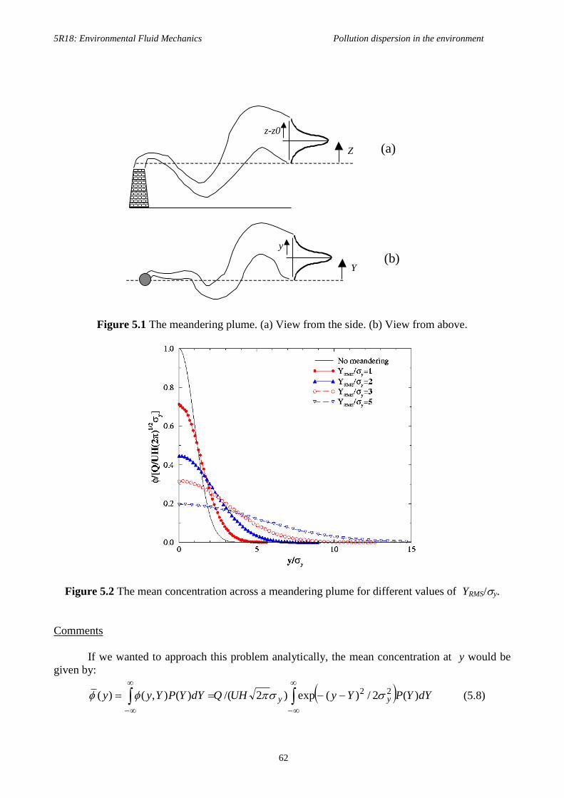
5R18: Environmental Fluid Mechanics Pollution dispersion in the environment
62
z-z0
Z (a)
y
Y (b)
Figure 5.1 The meandering plume. (a) View from the side. (b) View from above.
Figure 5.2 The mean concentration across a meandering plume for different values of YRMS/y.
Comments
If we wanted to approach this problem analytically, the mean concentration at y would be
given by:
dYYPYyUHQdYYPYyy yy )(2/)(exp)2/()(),()( 22
(5.8)

5R18: Environmental Fluid Mechanics Pollution dispersion in the environment
63
This is quite difficult to evaluate in closed form and if at all, it can be done only for simple forms of
the P(Y), the pdf of Y. It can be shown that for a Gaussian P(Y), )(y is given by an expression
identical to Eq. (4.20), but with an effective dispersion coefficient
222
, RMSymeandy Y (5.9)
This is typical of random, uncorrelated motions: the overall variance due to the action of two
phenomena (meandering, smaller-scale turbulent diffusion) is the sum of the variances due to each
phenomenon alone. (This concept is also used in experimental error estimation.) The basic
assumption behind the flapping model presented previously is that the turbulent diffusion motions
resulting in Eq. (4.20) are uncorrelated from the large-scale motions causing the meandering.
However, in real atmospheric turbulence, the scales causing mixing of the plume are not fully
independent from the motions causing the meandering. Hence, the discussion above should be seen
as only an approximation to a real plume exposed to sudden, strong, cross winds.
Equation (5.8) cannot be easily evaluated analytically for other shapes of the pdf of Y.
However, the stochastic simulation does not have this restriction and it also gives access to the full
pdf of , which is very useful for predicting the fluctuations of pollutant at a particular point.
5.4 Worked examples
Example 5.1
On a particular day, the air above a city is completely still. A box model (Section 4.1) is
here extended to account for small-scale turbulent fluctuations in the concentrations that are a
function of time. Assume that there are no emissions and that the pollutant is inert with
homogeneous mean concentrations in all directions, but that there are significant fluctuations at t=0.
Hence, simplify and solve Eq. (3.16). The turbulence lengthscale is Lturb=50 m and the turbulence
velocity is u= 0.1 m/s. Calculate the rms after 5 min as a fraction of the initial rms 0.
Solution
When there are no spatial inhomogeneities, Eq. (3.12) becomes
consttzyxdt
dw
xD
xxu
t jT
jjj
),,,(0
, as expected. The equation
for the variance (Eq. 3.16, using Eq. 3.17) becomes: 2
2 '2
turbL
u
dt
d . Integrating this equation
gives: turbTt /2exp2
02 , with '/ uLT turbturb . This is an exponential decay to zero from
the initial value of 0. This shows that the inert scalar fluctuations will have decayed to 1/e their
initial value over one half turbulence timescale and that they will have essentially disappeared after
three turbulence times. For the conditions given, Tturb=500 s, and hence /0=0.3. Note the quick
disappearance of the fluctuations in atmospheric turbulence, e.g. of the order of minutes. This is
consistent with everyday experience.

5R18: Environmental Fluid Mechanics Pollution dispersion in the environment
64
Example 5.2
Repeat Ex. 5.1, but now assume (a) that the pollutant is photolysed at a rate –Jc, where J is a
constant and c the pollutant concentration; (b) that the pollutant is destroyed at a rate –Jc2.
Solution
In this Example, the mean concentration is changing with time due to the chemistry and we
need to include the fluctuations in the chemical source term.
(a) The governing equation becomes: JtcccJJcdt
cdw
dt
cd exp)0( .
The corresponding equation for the reacting scalar variance is now
J
TccJ
Twc
L
u
dt
d
turbturbturb
122
22
'2 222
2
. The solution is easily
obtained as: )2exp(/2exp2
02 JtTt turb . So now the decay of the fluctuations depends on
the turbulence and on the chemistry. If the initial mean concentration is C, an appropriate chemical
timescale is C/J. We can then define a Damköhler number as Da=JTturb/C. If C/J>>Tturb (i.e.
Da<<1), we have intense turbulence and the fluctuations will have decayed to zero well before the
reaction is felt. On the other hand, if C/J<<Tturb, the fluctuations decay because the reactant is
consumed ( 0c ) according to the chemical timescale and the turbulence plays little role. This
Examples clearly demonstrates the Damköhler number criteria in Section 5.1.
(b) In this case, we have non-linear chemistry and the system of equations becomes:
22 JcJdt
cdccJ
dt
cdw
dt
cd
cccJTdt
dwc
L
u
dt
d
turbturb
222
2'
2 22
22
322
42
cJcJTdt
d
turb
.
( 32222 2)2( cJccJwccccccJwwccJwwJcw ). It
is evident that we cannot proceed unless we supply a model for the third-order correlation.
This example shows how difficult the combined turbulence-reaction system can become
when the chemistry is non-linear. However, it also demonstrates the very useful conclusion that for
fast turbulence relative to the reaction ( 0Da ), we can safely assume that the reactants are well-
mixed ( 0 ). Virtually all Air Quality Models in practice are based on this assumption, which is
used without much thought even if Da is not very small due to the large simplification it offers.
5R18: Environmental Fluid Mechanics Pollution dispersion in the environment
65
6. Summary and main points
The main objectives of these Notes have been:
(i) To describe the nature of some common atmospheric pollutants and their chemical
evolution.
(ii) To introduce techniques to describe the statistical nature of scalars and the mixing
encountered in turbulent flows.
(iii) To present the standard approaches currently in use by environmental regulation
agencies for predicting the concentration of pollutants above cities or downwind of
pollution sources.
(iv) To emphasize that the present status of modelling of turbulent reacting flows in the
environment include significant uncertainties because perfect mixing is usually assumed.
This is sometimes improper for non-linear chemistries, such as that of environmental
pollution, but it is correct if the chemistry is slow relative to the turbulence.
(v) To familiarize the student with Monte Carlo simulations because they are an extremely
powerful tool when dealing with stochastic phenomena like turbulence.
The most important points in these Notes are the following:
(i) Sections 2.2 and 2.3, where common pollutants and their chemistry are presented.
(ii) Equations (3.8) and (3.9) for the instantaneous and mean scalar.
(iii) The eddy diffusivity and Eq. (3.12).
(iv) The equation for the variance (3.16) and the model in Eq. (3.17).
(v) The source term problem (Eq. 3.19).
(vi) The concept of the probability density function.
(vii) Equation (3.22), definitions of the mean, rms and variance (Section 3.3).
(viii) The example in Section 3.3.
(ix) The box model, Section 4.1
(x) The Gaussian plume, Eq. (4.16), and the ground concentration, Eqs. (4.18, 4.19).
(xi) The use of Fig. 4.4 for the dispersion coefficients.
(xii) The difference between fast and slow chemistry (Section 5.1).
(xiii) The concept of the Monte Carlo simulation (Section 5.2).

5R18: Environmental Fluid Mechanics Pollution dispersion in the environment
66
5R18: Environmental Fluid Mechanics
Part II: Dispersion of Pollution in the Atmospheric Environment
DATA CARD
Transport equation for the mean of the reactive scalar :
wx
Kxx
ut jjj
j
Transport equation for the variance of the reactive scalar :
wgTx
Kx
gK
xx
gu
t
g
turbjjjjj
2
22
2
Mean concentration of pollutant after instantaneous release of Q kg at t=0:
zyxzyxK
zz
K
yy
K
xx
tKKKt
Qtzyx
20
20
20
2/12/3
)()()(
4
1exp
)()(8),,,(
Gaussian plume spreading in two dimensions from a source at (0,0,z0) emitting Q kg/s:
2
20
2
2
22exp
1
2),,(
zyzy
zzy
U
Qzyx
One-dimensional spreading from line source emitting Q/L kg/s/m :
2
2
2exp
2
1),(
yy
y
UL
Qyx
Relationship between eddy diffusivity and dispersion coefficient:
KU
x22

5R18: Environmental Fluid Mechanics Pollution dispersion in the environment
67
Stability categories and empirical data on dispersion coefficients:
A to F refer progressively from the very unstable to the very stable conditions, with D the neutral.
Wind speed
at 10 m high
(m/s)
Day Night
Solar intensity
Strong Moderate Slight Overcast Clear
0-2 A A-B B - -
2-3 A-B B C E F
3-5 B B-C C D E
5-6 C C-D D D D
> 6 C D D D D
Horizontal

5R18: Environmental Fluid Mechanics Pollution dispersion in the environment
68
Vertical


![ESD.864 Lecture Notes, Air pollution science and models · #12: Air Pollution Science and Models ESD.864 ... [Interview, 1998] ... assessment modeling done through IIASA,](https://static.fdocuments.in/doc/165x107/5b7b58797f8b9a184a8c758c/esd864-lecture-notes-air-pollution-science-and-models-12-air-pollution-science.jpg)