Aid and Growth at the Regional Level; by Axel Dreher and ... · ADM2 regions from 21 countries....

WP/15/196

IMF Working Papers describe research in progress by the author(s) and are published to elicit comments and to encourage debate. The views expressed in IMF Working Papers are those of the author(s) and do not necessarily represent the views of the IMF, its Executive Board, or IMF management.

Aid and Growth at the Regional Level

by Axel Dreher and Steffen Lohmann

© 2015 International Monetary Fund WP/15/196

IMF Working Paper

Research Department and Strategy, Policy, and Review Department

Aid and Growth at the Regional Level*

Prepared by Axel Dreher and Steffen Lohmann

Authorized for distribution by Andrew Berg and Catherine Pattillo

August 2015

Abstract

This paper brings the aid effectiveness debate to the sub-national level. We hypothesize the non-

robust results regarding the effects of aid on development in the previous literature to arise due to

the effects of aid being insufficiently large to measurably affect aggregate outcomes. Using geo-

coded data for World Bank aid to a maximum of 2,221 first-level administrative regions (ADM1)

and 54,167 second-level administrative regions (ADM2) in 130 countries over the 2000-2011

period, we test whether aid affects development, measured as nighttime light growth. Our

preferred identification strategy exploits variation arising from interacting a variable that indicates

whether or not a country has passed the threshold for receiving IDA's concessional aid with a

recipient region's probability to receive aid, in a sample of 478 ADM1 regions and almost 8,400

ADM2 regions from 21 countries. Controlling for the levels of the interacted variables, the

interaction provides a powerful and excludable instrument. Overall, we find significant

correlations between aid and growth in ADM2 regions, but no causal effects.

JEL Classification Numbers: F35, O19, O47

Keywords: Aid Effectiveness, Geo-coding, World Bank

Author’s E-Mail Address: [email protected], [email protected]

goettingen.de

* This paper is part of a research project on macroeconomic policy in low-income countries supported by the U.K.’s

Department for International Development (DFID). The paper was presented at the IMF/CFD Conference on

“Financing for Development” (Geneva, Switzerland, Jan 15–17, 2017) and is forthcoming in a Oxford Review of

Economic Policy special issue on financing for development. The views expressed herein are those of the authors and

should not be attributed to the IMF, its Executive Board, or its management, or DFID. We thank Andrea Presbitero,

seminar participants at the Development Research Group meeting at the University of Goettingen, the Conference on

Financing for Development (Geneva 2015), and the Centre for the Studies of African Economies Conference (Oxford

2015) for helpful comments, and Jamie Parsons for proofreading.

IMF Working Papers describe research in progress by the authors and are published to

elicit comments and to encourage debate. The views expressed in IMF Working Papers are

those of the authors and do not necessarily represent the views of the IMF, its Executive Board,

IMF management, or DFID.

mailto:[email protected]



Contents Page

1. Introduction ................................................................................................................................3

2. Data and Method ........................................................................................................................5

3. Results ...................................................................................................................................... 17

4. Conclusion ................................................................................................................................ 29

Appendix

Table A.1: Description of key variables .................................................................................... 38

Table A.2: Descriptive Statistics, ADM1, Estimation sample (2000-2012) .............................. 39

Table A.3: Specification at country-level, 2000-2012 ............................................................... 39

Figures

Figure 1. Location-specific World Bank disbursements in Africa ..............................................8

Figure 2. Raw versus intercalibrated nighttime light, 2000-2012 ............................................. 12

Figure 3. Regional growth in Africa, ADM1 regions, 2000-2002 to 2003-2005 ...................... 13

Figure 4. Change in location-specific disbursements after IDA income threshold crossing ..... 16

Tables

Table 1. OLS and Region-Fixed Effects, ADM1, 2000-2012 ................................................... 19

Table 2. OLS and Region-Fixed Effects, ADM2, 2000-2012 ................................................... 20

Table 3. 2SLS estimates using rainfall as IV, 2000-2011 .......................................................... 23

Table 4. 2SLS estimates based on the IDA income threshold crossing, ADM1, 2000-2012 .... 25

Table 5. 2SLS estimates based on the IDA income threshold crossing, ADM2, 2000-2012 .... 26

Table 6. Analysis by continents, 2000-2012 .............................................................................. 27

1 Introduction

Consider Malawi’s recent World Bank-sponsored Rural Land Development Project. In line

with its objectives, the project succeeded in increasing the incomes of about 15,000 poor rural

families in the project districts.1 Overall, the Bank’s Independent Evaluation Group (IEG)

rates around 75 percent of the World Bank’s projects as successful.2 Still, these projects do

not seem to measurably increase economic growth at the country level, as indicated by the lack

of robustness in empirical studies on the effectiveness of foreign aid.3 This striking disparity

between micro-level effectiveness and macro-level ineffectiveness is persistent in the empirical

literature and has been coined the micro-macro paradox in foreign aid (Mosley, 1987).

We argue that the previous literature’s focus on country- rather than regional-level growth in

incomes is one important reason for the lack of a robust effect of aid on growth.4 While Malawi’s

World Bank project may increase the incomes of people in some of the targeted areas, it is

unlikely that the increase in incomes is sufficiently large to be measurable at the country level.

This arguably holds when we consider the total of Malawi’s projects. According to data from

AidData, total geo-coded aid inflows to Malawi amounted to almost 5.3 billion US dollars over

the 2004-11 period (Peratsakis et al., 2012; Rajlakshmi, 2013).5 However, the regional allocation

of this aid is not uniform across Malawi. For instance, the North receives fewer projects than

the South, and aid projects cluster in densely populated areas.6 While these projects may fail

to measurably promote growth in all of Malawi, the effects of aid might well be discernable at

a more disaggregated level.

The lack of evidence on aid effectiveness at the regional level is due to the dearth of available

data and the methodological problems in measuring the causal effect of aid below the country-

level. With data availability increasing as a consequence of AidData’s (and selected recipient

countries’) geo-coding efforts of aid projects,7 some recent studies have looked at the regional

allocation of aid. However, with the exception of two studies focusing on Malawi,8 aid’s effect on

1See http://ieg.worldbankgroup.org/Data/reports/PPAR-75556-P132257-Malawi_Land_Dvlpmt.pdf (ac-cessed March 16, 2014). The project was approved in 2004, and closed in 2011.

2See Dreher et al. (2013).3E.g., Rajan and Subramanian (2008); Doucouliagos and Paldam (2009); Bjørnskov (2013); Roodman (2015).4Another reason, of course, is the lack of a credible identification strategy. We return to this below.5This represents around 80 percent of total World Bank commitments there. It amounts to 16 percent of

Malawi’s GDP over the same period.6See AidData’s blog entry on Malawi of April 19, 2012, http://aiddata.org/blog/where-are-donors-

working-in-malawi-a-new-dataset-sheds-light (accessed March 19, 2014).7See Strandow et al. (2011) and AidData (2015).8See Rajlakshmi (2013) and Dionne et al. (2013).

3

http://ieg.worldbankgroup.org/Data/reports/PPAR-75556-P132257-Malawi_Land_Dvlpmt.pdf

http://aiddata.org/blog/where-are-donors-working-in-malawi-a-new-dataset-sheds-light

http://aiddata.org/blog/where-are-donors-working-in-malawi-a-new-dataset-sheds-light

growth has so far not been analyzed at the sub-national level.9 With geo-coded data on World

Bank aid now being made available, we are able to conduct such an analysis.10

The lack of systematic empirical evidence on the effectiveness of aid below the country-level is

an important gap in the literature. As we explain in detail in section 2, we aim to fill this gap by

making use of geo-coded data for 1,662 World Bank aid projects in 2,221 first-level administrative

regions (ADM1) and 54,167 second-level administrative regions (ADM2) in 130 countries that

were approved over the 2000-2011 period.11 We test whether and to what extent disbursements

of this aid and the number of World Bank projects affect development, measured as nighttime

light growth. Given that we are the first to investigate the regional effectiveness of aid in

promoting growth for a large sample of recipient countries, we start by replicating two prominent

identification strategies from the country-level literature as closely as possible. First, we follow

the recent analysis of Clemens et al. (2012), who address the potential endogeneity of aid by

removing country-specific factors that do not vary over time, allowing for a time lag between

the disbursement of aid and growth, and focusing on aid that they assume is particularly likely

to affect growth in the short-run – so-called early-impact aid. Second, we rely on Bruckner

(2013), who suggests using, inter alia, rainfall growth and its square to purge aid of that part

that is driven by changes in GDP per capita. As we explain below, these approaches cannot

fully address concerns regarding the endogeneity of aid, and thus not necessarily allow us to

identify a causal effect. What is more, rainfall turns out to be weak as an instrument for growth

in our sample in most specifications.

Our own approach to identify the causal effect of aid on growth is closely connected to recent

innovations in the country-level literature on aid effectiveness. We rely on Galiani et al.

(2014), who instrument aid inflows with the income threshold of the International Development

Association (IDA) for eligibility to the World Bank’s concessional aid. This instrument could

arguably be correlated with growth for reasons other than aid (Dreher and Langlotz, 2015). We

overcome this problem by interacting the indicator of whether or not a country has crossed the

IDA’s threshold for receiving concessional aid with a recipient region’s probability to receive

aid, following recent identification strategies in the country-level literature on aid effectiveness

(Werker et al., 2009; Ahmed, 2013; Nunn and Qian, 2014; Chauvet and Ehrhart, 2014; Dreher

9Chauvet and Ehrhart (2014) employ the World Bank’s Enterprise Surveys to examine how aid affects thegrowth of firms in 29 developing countries. While they do not use geo-coded aid, this allows them to combinecountry-level and firm-level characteristics, potentially mitigating reversed causality.

10Of course, we would like to test the effectiveness of aid from a larger sample of donors. Such data are notavailable for a worldwide sample.

11ADM1 regions are the governmental units directly below the nation state; ADM2 regions are those below theADM1 level.

4

and Langlotz, 2015).12 Controlling for the levels of the interacted variables, the interaction

provides a powerful and excludable instrument.

According to our results (shown in section 3), aid and nighttime light growth are significantly

correlated at the second-level administrative areas (ADM2) level, but not at the larger first-level

administrative areas (ADM1) level. Specifically, when we do not employ instruments, lagged

aid shows a positive and significant correlation when region-fixed effects are not included in the

specification, but a negative correlation otherwise. Purging aid of its endogenous component

relying on rainfall growth and its square, we find the instruments to be weak in most specifica-

tions. The exception is at the ADM2 level, where we find a negative effect of aid on growth in

our region-fixed effects specification. However, given the strong identifying assumption that this

result relies on, we advise caution in interpreting it. When we employ our preferred instrument

– the interaction of the probability to receive aid with having passed the IDA income threshold

– in a sample of 478 ADM1 regions and almost 8,400 ADM2 regions in 21 countries, we find no

effect of aid on development.

We conclude that there is no robust evidence showing that aid increases growth and discuss

implications for future research in the final section of the paper.

2 Data and Method

The literature on the allocation and effectiveness of foreign aid below the country-level is scarce,

mainly due to a lack of geo-coded data on aid, relevant outcomes, and adequate control variables.

A number of datasets exist however which allow testing for sub-national determinants and conse-

quences of aid. The dataset covering the largest number of countries has recently been provided

by AidData (2015) in collaboration with the World Bank and consists of 3,534 geo-coded World

Bank projects spread over 141 countries, approved over the 2000-2011 period.13 AidData also

provides geo-coded information on projects from the African Development Bank (AfD) approved

in the 2009-2010 period.14 Dreher et al. (2014) provide geo-coded data on Chinese aid to Africa,

12Werker et al. (2009) rely on an interaction between oil prices and Muslim majority countries to instrumentfor oil-producing donors’ aid, Ahmed (2013) and Dreher and Langlotz (2015) interact donor-level politicalfractionalization (which induces increases in donors’ aid budgets) with the probability of a recipient countryto get aid, while Nunn and Qian (2014) interact the probability to receive aid with US wheat production (toinstrument for food aid from the United States). Chauvet and Ehrhart (2014) interact donor government revenuewith cultural and historic distance between the donor and the recipient.

13See Findley et al. (2011) for a detailed description of an earlier – partial – release of these data.14The World Bank- and AfD-data have been used in a number of aid allocation studies. Ohler and Nunnenkamp

(2014) use an earlier subset of these data to study what determines the allocation of aid across a sample of27 recipient countries over the 2005-2011 period. Variants of these data have also been used to study thedeterminants of aid allocation in Nunnenkamp et al. (2012) for India, Jablonski (2014) for Kenya, and Powell andFindley (2012) for six Sub-Sahara African recipient countries. Zhang (2004) relies on data provided by the WorldBank to investigate the determinants of World Bank project allocation across Chinese provinces.

5

for the 2000-2012 period.15 Cambodia and Malawi share detailed information on the regional

allocation of the aid they receive from a large number of donors.16

For this project, we make use of AidData’s geo-coded data for World Bank projects – the only

data available for a worldwide sample of countries over a reasonably long period of time. The

raw dataset contains the project’s date of approval, the (anticipated) date of termination, and

the amounts committed to and disbursed in the project over its entire duration. To calculate

project-specific annual disbursements, we link the project database to the Bank’s documentation

of project-specific financial flows, including the precise date of project disbursements.17 We

transform these disbursements into constant 2011 US$. A second variable of interest is the

number of active projects per region rather than amounts of aid. This variable is frequently

used in the literature trying to quantify the effects of World Bank involvement, as it might

more adequately measure other components that accompany a project, like technical advice or

program conditions, than do the amounts of aid alone (Boockmann and Dreher, 2003).

AidData covers projects that have been approved over the 2000-2011 period, comprising total

commitments of nearly 370 bn US$. For each project, detailed information on its locations

is recorded, with different degrees of precision: Some projects are implemented in a limited

geographical area, such as a village or city. Others are realized at more aggregate levels, such

as a municipality, a district or greater administrative region. As described in detail in Findley

et al. (2011) and Strandow et al. (2011), the geo-coding is implemented by experienced coders

in a double-blind process. Information on project locations come from various World Bank

sources, most importantly project-specific planning or implementation documents. In a next

step, coordinates of these locations are extracted from geographic online services providing

names and coordinates of administrative divisions, populated areas, and other places of interest.

Obviously, the coding precision reflects the sectoral composition of aid. Projects in sectors such

as “Finance” or “Public Administration, Law, and Justice” are geo-coded predominantly at the

national scale, while projects in sectors like “Transportation” are typically assigned to more

15Their results show that African regions where the current leader of a country was born receive substantialincreases in aid from China, but – controlled for region-fixed effects – not from the World Bank.

16Ohler (2013) uses these data to investigate whether and to what extent donors coordinate at the regional levelin Cambodia; Rajlakshmi (2013) and Dionne et al. (2013) investigate the allocation of projects from 30 donoragencies in Malawi.

17These data are available at the World Bank’s project website (http://www.worldbank.org/projects) perproject, but not in aggregate form. We downloaded these data and aggregated disbursement flows on a yearlybasis, treating negative disbursements as zero. In contrast to Dionne et al. (2013) we therefore do not need toestimate actual disbursements based on commitments or make restrictive assumptions on the spread of financialflows over the duration of a project. We provide our disbursement data at http://aiddata.org/replication/

worldbankdisbursements.

6

http://www.worldbank.org/projects

http://aiddata.org/replication/worldbankdisbursements

http://aiddata.org/replication/worldbankdisbursements

precise locations.18

In total, close to 48 percent of all project locations geo-coded by AidData are assigned to a

distinguishable subnational location. Since this paper focuses on sub-national projects’ effects on

sub-national growth, we exclude projects that are nation-wide in scope, for which no or unclear

information on location is provided, and projects that are directly allocated to a government

entity, as these cannot be attributed to specific regions.19

We use the available project information on longitude and latitude of respective locations to

match the aid projects to the respective country’s first and second Administrative Regions

(ADM1 and ADM2) using data from the Global Administrative Areas (GADM) database.20

ADM1 regions are the governmental units directly below the nation state, such as counties,

regions, provinces, municipalities, or districts, among others, depending on the particular coun-

try (see Figure 1 for the African continent). ADM2 regions are those regions that are directly

below the ADM1 level, like districts, municipalities, and communes. Regarding the matching to

ADM1 regions, 77 percent of the projects were implemented in more than one region, without

information on the share of aid disbursements going to the particular sites. For ADM2 regions,

this concerns 88 percent of the projects. Following the previous literature (e.g., Dionne et al.,

2013), we assume that aid (disbursements and number of projects) is allocated in proportion to

the size of an area’s population.21

Population data are taken from CIESIN/CIAT’s “Gridded Population of the World” (CIESIN,

2005). These data are available for a worldwide grid of 2.5 arc-minutes resolution for the years

2000, 2005, and 2010. We calculate population size per administrative region by taking its

mean population density and multiplying it with the area size provided in the GADM file. We

use linear interpolation for the missing years, given that population changes slowly over time.

Figure 1 shows the sum of aid disbursements per-capita over the whole 2000-2011 period for

ADM1 regions of Africa. The figure illustrates the wide range of aid-receipts at the regional

18The “Tamil Nadu Road Sector Project” in India as one typical infrastructure project, for example, aims topromote the core road network of Tamil Nadu through upgrading existing state highways, maintaining smallerstate roads, and institutional strengthening. In the dataset, twelve geo-coded locations are assigned to the projectof which six correspond to an exact location, such as a village or town, five to ADM2 regions, and one to anADM1 region. Malawi’s “Rural Land Development Project,” introduced above, in turn could only be assignedmore broadly to five smaller administrative divisions.

19In the empirical analysis, any potential country-wide effects of these flows are absorbed through the inclusionof country-period fixed-effects.

20See http://www.gadm.org.2123% (12%) of the projects are located in one ADM1 (ADM2) region exclusively, 37% (25%) have locations

in between 2-5 regions, 21% (19%) in 6-10 regions, and 18% (44%) in at least 10 regions. We test robustness bydividing aid amounts and numbers equally per project location, as in Dreher et al. (2014). Our conclusions arenot affected by this.

7

http://www.gadm.org

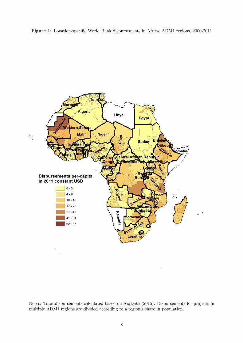
Figure 1: Location-specific World Bank disbursements in Africa, ADM1 regions, 2000-2011

Sudan

Algeria Libya

Mali

Chad

Niger

EgyptAngola

EthiopiaNigeria

South Africa

Namibia

Tanzania

Maurita

nia

Zambia

Kenya

Somalia

Congo (Democratic Republic of the)

Mozambique

Botswana

Morocco

Congo

Cameroon

Zimbabwe

Gabon

GhanaGuinea

Uganda

Tunisia

Côte d'IvoireCentral African Republic

Burkina FasoEritrea

Western Sahara

Malawi

Liberia

Lesotho

BurundiRwanda

DjiboutiBeninTogo

Disbursements per-capita,in 2011 constant USD

0 - 34 - 910 - 1617 - 2627 - 4041 - 6162 - 87

Notes: Total disbursements calculated based on AidData (2015). Disbursements for projects inmultiple ADM1 regions are divided according to a region’s share in population.

8

level within some (but not all) African countries, emphasizing the importance of investigating

the effects of aid at the regional level.22

As is common in the literature on aid effectiveness, we average our data to smooth changes

over the business cycle. We follow Galiani et al. (2014) and build averages over three years.

This is useful for our preferred identification strategy below, as donors commit funds to the

IDA in so-called replenishment rounds that span these three-year periods.23 Our reduced-form

empirical models are at the region-period level:

Growthi,t = α+ βAidi,t−1 + δDEV i,2000 + ζPOP i,t−1 + θPOPGROWTH i,t

+ ρAREAi + µDIST i + ηc,t + εi,t (1)

Growthi,t = α+ βAidi,t−1 + ζPOP i,t−1 + θPOPGROWTH i,t + ηc,t + λi + εi,t, (2)

where i denotes regions and c countries. Growthi,t measures region i’s average annual growth

rate in nighttime light over period t − 1 to t. Aidi,t−1 denotes the natural logarithm of annual

per-capita aid disbursements in constant 2011 US$ or – alternatively – the number of projects

per capita with ongoing disbursements to the region in the previous period.24 All regressions

include fixed effects for each country in each period (ηc,t). Model (1) in addition controls for

DEV i,2000 – the (logged) level of a region’s development (measured in nighttime light) at the

beginning of our sample period, to control for conditional growth convergence. It includes POP

and POPGROWTH, which are the logarithm of a region’s population size and its population

growth rate, AREA, reflecting the size of the administrative region, and DIST , measuring the

(logged) shortest distance from the region’s center to the country’s capital. It is sometimes

argued that population and area size affect growth, either negatively due to less diversified

economies and higher exposure to external risk or positively, due to increases in productivity

(Easterly and Kraay, 2000). Regarding distance to the country’s capital, we hypothesize more

distant regions to experience lower rates of growth.

22For they can be clearly identified as outliers in partial leverage plots, we remove the upper and lower 1th-percentiles of all aid variables from the sample.

23Specifically, we average data over the periods 2000-02, 2003-05, 2006-08, 2009-11, matching the IDA’sreplenishment rounds. We also include light data for the year 2012 to gain an additional “period,” given that aidenters the regressions with a lag.

24We add 0.01 before we take logs to avoid losing observations without disbursements or projects. Note that wealso take the number of projects in per-capita terms. Our conclusions hold, however, when taking the absolutenumber of projects per region. We follow Galiani et al. (2014) and include logged aid rather than the level ofaid along with its square, as do, e.g., Clemens et al. (2012). The reason is that we mostly rely on results frominstrumental variable estimation but only have one instrument for two endogenous variables in case we includeaid squared. Taking the log allows for a decreasing marginal effect of aid (but does not allow its effect to changesign).

9

Model (2) includes fixed effects for regions λi in addition to those for country-periods, and

therefore excludes control variables that do not vary over time at the regional level. Model (1)

consequently identifies the potential effect of aid exploiting variation between regions (and over

time), while Model (2) exploits within-region variation over time exclusively. While being

more conservative than Model (1), this comes with the disadvantage of few three-year-period

observations per region, which makes the identification of significant effects less likely. The error

term is εi,t, and we cluster standard errors at the regional level.

Our measure of development relies on nighttime light data as an approximation of regional

economic activity. Such data have been introduced to the literature in Elvidge et al. (1997)

and Sutton and Costanza (2002), and are frequently used in the recent economics literature

(probably most prominently in Henderson et al., 2012). Nighttime light is a practical source

of data for regional economic activity when official data on GDP are unavailable or where

official statistics might be prone to measurement error or manipulation (Chen and Nordhaus,

2011).25 Particularly in the developing world, uncertainty about official GDP estimates can be

enormous (Henderson et al., 2012; Jerven, 2013).26 A substantial number of studies has show

the correlation between nightlight and GDP to hold at the sub-national level, for regions of

varying size and levels of development.27

Since a large part of economic activity comes in the form of consumption and production using

light in the evenings, nighttime light intensity can be considered a meaningful reflection of human

economic activity. A range of studies have established a strong empirical relationship between

nighttime light intensity and GDP both over time and across regions. Recently, Henderson et al.

(2012) document a high correlation between changes in nighttime light intensity and GDP growth

at the country-level while Doll and Morley (2006) and Hodler and Raschky (2014) provide

similar regional-level evidence. Further research also finds strong positive associations between

nighttime light intensity and public infrastructure indicators (Michalopoulos and Papaioannou,

2014) as well as composite wealth indices from Demographic and Health Surveys (DHSs) (Noor

et al., 2008; Michalopoulos and Papaioannou, 2013), both at the national and the subnational

25Since nighttime light data are not directly relevant to governments, they are less likely to be systematicallytargeted by policy interventions.

26See http://qz.com/139051/nigerias-economy-is-about-to-grow-40-in-one-day/#139051/nigerias-

economy-is-about-to-grow-40-in-one-day for a case from Nigeria (accessed March 19, 2014).27See Doll and Morley (2006); Bhandari and Roychowdhury (2011); Hodler and Raschky (2014); Mveyange

(2015); Olivia and Stichbury (2015). Any structural differences between regions that do not vary over time acrossregions will be captured by region-fixed effects in our preferred estimations.

10

http://qz.com/139051/nigerias-economy-is-about-to-grow-40-in-one-day/#139051/nigerias-economy-is-about-to-grow-40-in-one-day

http://qz.com/139051/nigerias-economy-is-about-to-grow-40-in-one-day/#139051/nigerias-economy-is-about-to-grow-40-in-one-day

level.28

We use satellite images from the National Oceanic and Atmospheric Administration (NOAA,

nd), providing information on nighttime light activity for the 1992-2012 period. Images are taken

in the evenings, for a global grid in 30 arc-minutes resolution, and measured on a 0-63 scale

(with larger values indicating more activity). The data remove background noise and exceptional

events such as fires. They are, however, not directly comparable over time. The reason is that

the data included in our sample are generated with three different satellites and consequently

different sensors. What is more, sensors deteriorate with time, so that images from periods too

far apart might hardly be comparable (Elvidge et al., 2014). We therefore rely on recalibrated

data provided by Elvidge et al. (2014) at the country-year level, and adjust our regional nighttime

light data according to a region’s share in total light.29 Figure 2 compares yearly totals of

nighttime light intensity values for the regions in our sample with the recalibrated data. As can

be seen, the recalibration method smoothes nighttime light substantially, both between satellites

and in the years where data are generated by the same satellite, but where sensor sensitivity

changes over time.

Our proxy for regional development is calculated as the growth rate of (recalibrated) mean

nighttime light intensity in a region and year. We removed the upper and lower 5th-percentiles

from the sample, which can be clearly identified as outliers in partial leverage plots based on our

baseline specification.30 Figure 3 shows the resulting growth in average nighttime light intensity

over the 2000/02-2003/05 period for Africa at the ADM1 level. Table A.1 in the Appendix

shows the sources and definitions of all variables, while Table A.2 reports descriptive statistics.

The scarce literature on the sub-national determinants of aid effectiveness provides interesting

evidence on the correlates of aid projects on the regional level, but fails to convincingly address

28Possibly, certain World Bank projects, particularly those aiming at infrastructure development, affect thismeasure through opening up construction sites lit at night. While such sources of light might be the result ofeconomic activity as in any aid effectiveness study, i.e., that of increasing investment, we also check whether ourresults are robust to the exclusion of those parts of aid. In a sensitivity analysis, we drop projects assigned tothe transportation sector (which, however, accounts for the largest share of projects). With the exception of theOLS regressions for ADM2 regions, where the coefficient loses significance, the results remain similar. For thisreason and since the identification of construction projects is inexact to some extent – the datasets only allowsthe identification of a broader sector – we refrain from overemphasizing this channel.

29The method relies on reference to a base area where nighttime light can be assumed to vary little over time,with the data range of other areas adjusted in accordance.

30Our results depend on this to some extent. When we do not remove outliers the correlation between aid andgrowth tends to be more negative.

11

Figure 2: Raw versus intercalibrated nighttime light, 2000-2012

F15 F16 F18

5010

015

020

0S

um o

f lig

hts

(in m

illio

n)

2000 2001 2002 2003 2004 2005 2006 2007 2008 2009 2010 2011 2012

Intercalibrated Raw

Notes: The vertical axis shows the annual sum of nighttime light pixel values throughoutour sample period for different satellites (F15/F16/F18). Intercalibrated data are based onadjustment factors taken from Elvidge et al. (2014), according to a region’s share in total light.

12

Figure 3: Regional growth in Africa, ADM1 regions, 2000-2002 to 2003-2005

Sudan

Algeria Libya

Mali

Chad

Niger

EgyptAngola

EthiopiaNigeria

South Africa

Namibia

Tanzania

Maurita

nia

Zambia

Kenya

Somalia

Congo (Democratic Republic of the)

Mozambique

Botswana

Morocco

Congo

Cameroon

Zimbabwe

Gabon

GhanaGuinea

Uganda

Tunisia

Côte d'IvoireCentral African Republic

Burkina FasoEritrea

Western Sahara

Malawi

Liberia

Lesotho

BurundiRwanda

DjiboutiBeninTogo

Average annualgrowth rate

-0.32 - -0.07-0.06 - -0.03-0.02 - -0.010.00 - 0.010.02 - 0.040.05 - 0.070.08 - 0.130.14 - 0.62

Notes: Growth in average nighttime light intensity (in percent) based on NOAA Version 4DMSP-OLS Nighttime Lights Time Series. Data have been calibrated based on Elvidge et al.(2014).

13

causality.31 We present results using three different identification strategies.32 First, we broadly

follow Clemens et al. (2012), not using any instrument for aid, but allowing aid to affect growth

with a time lag, and removing influences that do not vary over time (across countries and,

in our case, across regions). Clemens et al. categorize all aid into one of two categories, so-

called early- and late-impact aid.33 Early-impact aid contains those types of aid that can

reasonably be expected to affect growth in the short-term, like budget support and program aid

and certain categories of project aid (e.g., infrastructure investment or support for production in

transportation, agriculture and industry). We use the sector classification included in AidData’s

project database to characterize a project based on the major sector that it is assigned to.34

This identification strategy would be unable to identify a causal effect of aid to the extent that

donors (or recipients) are selective and allocate more aid to the regions they expect will use the

aid more effectively.

Second, we follow the approach of Bruckner (2013). Bruckner addresses the endogeneity of aid

by instrumenting for changes in per capita GDP with data on rainfall growth and its square and

international commodity price shocks in his aid allocation equation. He then uses that part of

aid that is not driven by GDP per capita growth as an instrument to identify the causal effect

of aid on per capita GDP. We broadly follow this approach at the regional level, using data

on rainfall from the Global Precipitation Climatology Centre (GPCC) of the German Weather

Service (Schneider et al., 2011).35 We do not include commodity price shocks because they do

not vary across regions and are therefore absorbed by our country-period fixed effects. The

31Rajlakshmi (2013) is the only study we are aware of that tries to address the endogeneity of aid belowthe sub-national level. Rajlakshmi investigates the allocation and effectiveness of geo-coded aid projects from30 agencies in Malawi over the 2004-2011 period. He identifies his instruments for the aid effectiveness regressionsbased on the significance of the variables included in his aid allocation regressions. The endogeneity of aid for theoutcome variables included in the aid allocation equation is not addressed; what is more, the exclusion restrictionof the instruments used in the aid effectiveness regressions is unlikely to hold (regional dummies and an indicatorfor rural regions are likely to affect disease severity via channels other than aid). His Propensity Score Approachis based on few variables and is thus likely to suffer from unobserved heterogeneity between the treatment andcontrol group.

32Alternative strategies to identify the effect of development aid on economic growth can broadly be groupedalong three lines (see Dreher et al., 2014). The first relies on instruments related to the size of the populationin the recipient country. The second uses internal instruments – the lagged levels and differences of aid – andestimates system GMM regressions. The third relies on insight from the literature on the allocation of aid anduses proxies for political connections between the donors and recipients as instruments. As Bazzi and Clemens(2013) show, the first two strategies are unlikely to allow the identification of causal effects, as both populationand lagged values of aid are likely to have direct effects on growth. While political connection-based instrumentsmight be more likely to be excludable, Dreher et al. (2014) show that political motives influence the effectivenessof aid, so that the effect of politically motivated aid (the Local Average Treatment Effect) cannot be generalizedto represent the effect of aid more broadly.

33This measure has however been shown not to be a robust predictor of growth (Rajan and Subramanian, 2008;Bjørnskov, 2013; Roodman, 2015).

34Early-impact aid includes agriculture/fishing/forestry, energy/mining, access to finance, industry/trade,information/communications, and transportation. Late-impact aid includes education, health and other socialservices, public administration, and water and sanitation.

35See ftp://ftp.dwd.de/pub/data/gpcc/html/fulldata_v6_doi_download.html (accessed March 19, 2014).These data are available over the 2000-2010 period.

14

ftp://ftp.dwd.de/pub/data/gpcc/html/fulldata_v6_doi_download.html

identifying assumption is the absence of a direct effect of rainfall growth on aid, other than via

its impact on incomes. As holds for Clemens et al. (2012), Bruckner’s identifying assumption

might easily be violated.

Our third strategy connects to recent work on aid effectiveness at the country-level, which we

are convinced could most plausibly identify a causal effect of foreign aid at the regional level

(in case there is any). Our approach builds on Galiani et al. (2014), who instrument aid inflows

with passing the IDA’s threshold for receiving concessional aid. As Galiani et al. explain, donors

pledge their contributions for three-year periods. The IDA threshold is updated annually, and

amounts to a GNI per capita of US$1,215 in the Bank’s fiscal year 2015. Countries that pass the

threshold are likely to see a substantial reduction in IDA lending, though they do not become

ineligible for IDA aid immediately (Galiani et al., 2014). Of course, the decrease in IDA aid

might be replaced by increases in other donors’ aid, in our case, those of the International Bank

for Reconstruction and Development (IBRD), in particular. However, Galiani et al. (2014) show

that other donors reduce their aid in line with IDA aid, rather than substituting for it.36 They

also show that after a country crosses the IDA-threshold, IDA aid to GNI drops by 92 percent,

on average. As can be seen in Figure 4, the pattern described in Galiani et al. (2014) is prevalent

in our data as well. On average, IDA-aid per capita decreases by 75 percent between the year

before we assume the threshold effect to materialize (i.e., six years after the threshold has been

passed) and the year thereafter. The figure also shows that the decrease in IDA aid is not

systematically offset by corresponding increases in IBRD funding.

The IDA income-threshold – even if it would be fully exogenous from a recipient country’s

perspective – could arguably be correlated with growth for reasons other than aid (Dreher and

Langlotz, 2015).37 As Galiani et al. (2014) explain, countries could pass the income threshold due

to a large positive shock that is reversed in later years.38 We overcome this potential shortcoming

by interacting the indicator of whether or not a country has passed the IDA threshold with a

recipient region’s probability to receive aid, following recent innovations in the country-level

literature on aid effectiveness (Werker et al., 2009; Ahmed, 2013; Nunn and Qian, 2014; Dreher

and Langlotz, 2015). As Nunn and Qian (2014, pp. 1632, 1638) explain, the resulting regressions

resemble difference-in-difference approaches, where – in our application of the method – we

36For more details on the relation between IDA aid and the income threshold, see Galiani et al. (2014). Knacket al. (2014) provide the years that countries crossed the IDA-threshold. Galiani et al. find that DAC aid decreasesby 59 percent after a country crosses the threshold.

37Of course, to the extent that aid-dependent countries are less likely to cross the threshold – “cooking theirbooks” – it might well be endogenous to aid; see Kerner et al. (2014) and Galiani et al. (2014) who come toopposite conclusions on whether or not manipulation takes place.

38They employ alternative instruments using a smoothed income trajectory to rule out the effect of shocks andfind similar results however.

15

Figure

4:

Ch

an

ge

inlo

cati

on-s

pec

ific

dis

bu

rsem

ents

afte

rID

Ain

com

eth

resh

old

cros

sin

g

-40

-30

-20

-10

010

Aid

dis

burs

emen

ts p

er-c

apita

, in

cons

tant

201

1 U

S$

Uzb

ekis

tan

Ukr

aine

Tur

kmen

ista

n

Sud

an

Sri

Lank

a

Rep

ublic

of C

ongo

Pap

ua N

ew G

uine

a

Nig

eria

Mon

golia

Mol

dova

Indo

nesi

a

Indi

a

Hon

dura

s

Egy

pt

Djib

outi

Chi

na

Cam

eroo

n

Bol

ivia

Bhu

tan

Aze

rbai

jan

Ang

ola

Sou

rce:

ow

n ca

lcul

atio

ns b

ased

on

Aid

Dat

a (2

015)

IDA

IBR

D

Not

es:

Th

egr

aph

show

sth

eco

untr

ies’

aver

age

diff

eren

cein

regi

on-s

pec

ific

aid

dis

bu

rsem

ents

bet

wee

nth

ep

erio

dp

rior

toth

eye

arw

hen

the

IDA

-th

resh

old

effec

tis

ass

um

edto

take

pla

ce(i

.e.,

six

year

saf

ter

the

inco

me

thre

shol

dis

pas

sed

)an

don

eye

ar

late

r.

16

compare regular aid recipients to irregular recipients as the recipient’s IDA status changes.39

While we report results employing the other two identification strategies described above in order

to be comparable with the existing literature at the country-level, we base our conclusions mainly

on this, preferred, approach. This comes at the cost of dismissing a large number of countries

from the sample, as we prefer to implement our identification strategy only for countries that

crossed the IDA-threshold at a point in time that is covered by our sample. The resulting number

of countries included here is 21, referring to 478 ADM1 and almost 8,400 ADM2 regions.40

Our assumed timing broadly follows the previous literature. Countries are considered as IDA gra-

duates after having been above the income threshold for three consecutive years (Galiani et al.,

2014). Galiani et al. therefore expect decreases in aid disbursements to take effect in the next

replenishment period rather than instantaneously and lag the instrument by one three-year

period. We add an additional three-year period lag, given that commitments are on average

disbursed with a delay, broadly in line with the timing suggested in Dreher et al. (2014).41 Note

that ten countries passed the threshold in the last or second-to last period in our sample. We

follow Galiani et al. (2014) and keep them in the sample, even though the instrument will be

zero for these countries throughout the sample period due to using the instruments in lags. We

calculate the probability of receiving aid as the number of years in all years that a region has

received any World Bank aid prior to when we assume the IDA-threshold effect to take place

(i.e., six years after the income threshold is passed).42

The next section reports our results.

3 Results

Table 1 shows the results for our first set of regressions at the ADM1 level, broadly following

Clemens et al. (2012). When region-fixed effects are excluded, nighttime light growth decreases

with the level of nighttime light in 2000 at the one-percent level of significance, indicating

within-country convergence in development. At the five-percent level, growth increases with the

39We tested for differences in growth across regions with a high compared to regions with a low probabilityto receive aid prior to passing the threshold and did not find significant differences. As do Galiani et al. weonly consider countries that crossed the threshold from below for the first time in constructing the instrumentalvariable. In our sample, only Bolivia passed the threshold twice. Our results are robust to using the secondcrossing instead of the first.

40This compares to 35 countries in Galiani et al. (2014).41Results are qualitatively similar when using a one-period lag.42The main analyses in Ahmed (2013) and Nunn and Qian (2014) calculate the probability to receive aid over

the whole sample period. Our second-stage results are similar when we follow this approach. The resulting firststage for ADM1 regions is substantially weaker however.

17

size of the regional population but is unaffected by population growth. More distant and smaller

regions grow less, at the one-percent level of significance.

Note that we have to exclude nighttime light in 2000, region size, and distance to the capital

when we control for region-fixed effects, as they do not vary over time. In these specifications

(Model 2 above), population is no longer significant at conventional levels, arguably due to its

low variation over time within region (aggravated by using linear interpolation to derive the

yearly data).

Columns 1 and 2 of Table 1 report results for (log) aid disbursements. As can be seen, aid has

no significant effect on growth. This holds regardless of whether region-fixed effects are excluded

(column 1) or included (column 2).43 The insignificant effect is easy to explain. To the extent

that aid is fungible, it might simply substitute for government expenditures that would have

flown to the region in the absence of any aid. The true effect of aid on growth in that particular

region would then indeed be zero.44 Another potential reason for the insignificant coefficient of

aid is reversed causality, even in the presence of lags. If crises and aid are persistent, higher aid

might be the effect of lower growth, biasing the coefficient of aid downwards.45 The coefficient

might then turn out to be insignificant, even if the true effect of aid is positive. Third, the low

number of periods and the resulting lack of variation might challenge the identification of aid’s

effect on growth. And finally, of course, the insignificant coefficient could reflect the absence of

an effect of aid on growth, even if the aid is not diverted to other regions.

Columns 3 and 4 of Table 1 replicate the analysis replacing aid disbursements with the number

of aid projects with positive disbursements, while columns 5-8 show regressions that separate

early-impact from late-impact aid, following Clemens et al. (2012). The results show insignificant

coefficients of aid in all specifications.

Table 2 replicates the analysis focusing on the smaller ADM2 regions. If our hypothesis that

more disaggregated analysis facilitates identification of significant effects holds true, we would

expect stronger effects here compared to the results in Table 1 above. To the contrary, focusing

43We separately included aid from the concessional International Development Association (IDA) and the lessconcessional loans from the International Bank for Reconstruction and Development (IBRD). The coefficientsare not significant at conventional levels. We also separated projects that have been successfully evaluated by theBank’s Independent Evaluation Group from those that have been not. Excluding region-fixed effects, growth isnegatively correlated with unsuccessful projects, at the ten-percent level of significance.

44Recipient governments might use their additional budgetary leeway to finance their own pet projects in otherregions – projects that cannot be identified and evaluated, but which potentially increase growth in the regionsthat get them. The same holds to the extent that positive spillovers increase growth in other regions, even absentany growth effects in the region that receives the aid.

45As Roodman (2015) shows, the procedure applied in Clemens et al. (2012) fails to remove contemporaneousendogeneity.

18

Table

1:

OL

San

dR

egio

n-F

ixed

Eff

ects

,A

DM

1,20

00-2

012

(1)

(2)

(3)

(4)

(5)

(6)

(7)

(8)

OL

SF

EO

LS

FE

OL

SF

EO

LS

FE

(Log)

Tota

laid

,t-

10.0

003

0.0

001

(0.0

007)

(0.0

011)

(Log)

No.

of

pro

ject

s,t-

10.0

006

0.0

009

(0.0

011)

(0.0

018)

(Log)

Earl

y-i

mp

act

aid

,t-

1-0

.0006

-0.0

017

(0.0

007)

(0.0

011)

(Log)

Late

-im

pact

aid

,t-

10.0

006

0.0

004

(0.0

008)

(0.0

012)

(Log)

No.

of

earl

y-i

mp

act

pro

ject

s,t-

10.0

001

-0.0

013

(0.0

012)

(0.0

019)

(Log)

No.

of

late

-im

pact

pro

ject

s,t-

10.0

006

0.0

005

(0.0

011)

(0.0

019)

(Log)

Nig

htt

ime

light

in2000

-0.0

142∗∗

∗-0

.0145∗∗

∗-0

.0141∗∗

∗-0

.0147∗∗

∗

(0.0

019)

(0.0

019)

(0.0

020)

(0.0

020)

(Log)

Siz

eof

pop

ula

tion

,t-

10.0

038∗∗

0.0

502

0.0

040∗∗

0.0

569

0.0

041∗∗

0.0

548

0.0

043∗∗

0.0

736

(0.0

019)

(0.0

526)

(0.0

019)

(0.0

529)

(0.0

019)

(0.0

531)

(0.0

019)

(0.0

531)

Pop

ula

tion

Gro

wth

0.0

870

0.9

221

0.0

903

1.0

924

0.0

865

0.9

565

0.1

211

1.2

207

(0.1

085)

(1.0

902)

(0.1

088)

(1.0

960)

(0.1

073)

(1.1

025)

(0.1

083)

(1.1

004)

(Log)

Are

a-0

.0056∗∗

∗-0

.0059∗∗

∗-0

.0058∗∗

∗-0

.0060∗∗

∗

(0.0

020)

(0.0

020)

(0.0

020)

(0.0

020)

(Log)

Dis

tan

ceto

cap

ital

-0.0

052∗∗

∗-0

.0052∗∗

∗-0

.0052∗∗

∗-0

.0053∗∗

∗

(0.0

012)

(0.0

012)

(0.0

012)

(0.0

012)

Reg

ion

-FE

No

Yes

No

Yes

No

Yes

No

Yes

Cou

ntr

y-P

erio

d-F

EY

esY

esY

esY

esY

esY

esY

esY

esN

um

ber

of

cou

ntr

ies

130

130

130

130

130

130

130

130

Nu

mb

erof

regio

ns

2221

2221

2214

2214

2219

2219

2213

2213

R2

0.2

90.4

70.2

90.4

70.2

90.4

70.2

90.4

7O

bse

rvati

on

s8541

8541

8519

8519

8469

8469

8470

8470

Note

s:O

LS

an

dre

gio

n-fi

xed

-eff

ects

regre

ssio

ns

(FE

).D

epen

den

tvari

ab

le:

Gro

wth

inn

ightt

ime

light.

All

vari

ab

les

are

aver

aged

over

3-y

ear-

per

iod

s.S

tan

dard

erro

rs,

clu

ster

edat

the

regio

n-l

evel

,in

pare

nth

eses

:*p<

0.1

,**p<

0.0

5,

***p<

0.0

1.

19

Table

2:

OL

San

dR

egio

n-F

ixed

Eff

ects

,A

DM

2,20

00-2

012

(1)

(2)

(3)

(4)

(5)

(6)

(7)

(8)

OL

SF

EO

LS

FE

OL

SF

EO

LS

FE

(Log)

Tota

laid

,t-

10.0

006∗∗

-0.0

012∗∗

(0.0

003)

(0.0

005)

(Log)

No.

of

pro

ject

s,t-

10.0

016∗∗

∗-0

.0011

(0.0

004)

(0.0

008)

(Log)

Earl

y-i

mp

act

aid

,t-

10.0

011∗∗

∗-0

.0005

(0.0

003)

(0.0

006)

(Log)

Late

-im

pact

aid

,t-

1-0

.0004

-0.0

016∗∗

(0.0

004)

(0.0

007)

(Log)

No.

of

earl

y-i

mp

act

pro

ject

s,t-

10.0

025∗∗

∗-0

.0004

(0.0

006)

(0.0

010)

(Log)

No.

of

late

-im

pact

pro

ject

s,t-

10.0

001

-0.0

023∗∗

(0.0

006)

(0.0

011)

(Log)

Nig

htt

ime

light

in2000

0.0

272∗∗

∗0.0

273∗∗

∗0.0

271∗∗

∗0.0

272∗∗

∗

(0.0

006)

(0.0

006)

(0.0

006)

(0.0

006)

(Log)

Siz

eof

pop

ula

tion

,t-

1-0

.0058∗∗

∗-0

.1234∗∗

∗-0

.0060∗∗

∗-0

.1220∗∗

∗-0

.0057∗∗

∗-0

.1249∗∗

∗-0

.0058∗∗

∗-0

.1207∗∗

∗

(0.0

006)

(0.0

149)

(0.0

006)

(0.0

150)

(0.0

006)

(0.0

150)

(0.0

006)

(0.0

151)

Pop

ula

tion

Gro

wth

0.1

293∗∗

∗-0

.1448

0.1

324∗∗

∗-0

.1707

0.1

326∗∗

∗-0

.2097

0.1

294∗∗

∗-0

.1558

(0.0

404)

(0.2

762)

(0.0

406)

(0.2

777)

(0.0

407)

(0.2

782)

(0.0

405)

(0.2

789)

(Log)

Are

a0.0

227∗∗

∗0.0

228∗∗

∗0.0

226∗∗

∗0.0

227∗∗

∗

(0.0

007)

(0.0

007)

(0.0

007)

(0.0

007)

(Log)

Dis

tan

ceto

cap

ital

-0.0

014∗∗

-0.0

015∗∗

∗-0

.0013∗∗

-0.0

014∗∗

(0.0

005)

(0.0

005)

(0.0

005)

(0.0

005)

Reg

ion

-FE

No

Yes

No

Yes

No

Yes

No

Yes

Cou

ntr

y-P

erio

d-F

EY

esY

esY

esY

esY

esY

esY

esY

esN

um

ber

of

cou

ntr

ies

130

132

130

132

130

132

130

132

Nu

mb

erof

regio

ns

54165

54167

54104

54106

54055

54057

54016

54018

R2

0.1

40.4

70.1

40.4

70.1

40.4

70.1

40.4

8O

bse

rvati

on

s195886

195893

195803

195808

194064

194071

194249

194253

Note

s:O

LS

an

dre

gio

n-fi

xed

-eff

ects

regre

ssio

ns

(FE

).D

epen

den

tvari

ab

le:

Gro

wth

inn

ightt

ime

light.

All

vari

ab

les

are

aver

aged

over

3-y

ear-

per

iod

s.S

tan

dard

erro

rs,

clu

ster

edat

the

regio

n-l

evel

,in

pare

nth

eses

:*p<

0.1

,**p<

0.0

5,

***p<

0.0

1.

20

on smaller regions will make it less likely to identify statistically significant effects if the main

reason for the lack of significant coefficients of aid is fungibility, and aid is more likely to be

diverted to areas close to the intended region. The results are strikingly different compared to

Table 1. First, note that with the exception of the distance to the country’s capital there are

substantial changes for all control variables. Growth increases with the level of nighttime light

in the year 2000, the region’s size and population growth (in the case where the region-fixed

effects are excluded from the regression), but decreases with the size of its population, all at the

one-percent level of significance.

As shown in column 1, when we do not control for region-fixed effects, growth significantly

increases with aid disbursements at the five-percent level. Conversely, when we include them

– in column 2 – growth decreases with aid, also at the five-percent level of significance. The

coefficient of column 1 shows that an increase in per capita aid by ten percent increases nighttime

light growth by 0.006 percentage points. With average disbursements in our sample amounting to

US$ 2.39 and an average population of 2.4 million, this amounts to additional aid in the order

of US$ 0.58 million. The corresponding decrease in growth according to column 2 is almost

twice as high. These numbers compare to an increase of 0.35 percentage points in GDP per

capita growth following a one-percentage point increase in the aid to GNI-ratio according to the

country-level results in Galiani et al. (2014) and an increase of 0.2 percentage points in Clemens

et al. (2012).

The results for aid broadly hold when we replace disbursements with the number of projects in

columns 3 and 4, though the negative coefficient in the fixed effects specification is no longer

significant at conventional levels.

Columns 5-8 separate early-impact aid from late-impact aid, as suggested in Clemens et al.

(2012). The results are indeed substantially more positive for early-impact aid compared to

late-impact aid. When we exclude region-fixed effects, growth increases with early-impact aid

(columns 5 and 7), with a coefficient roughly twice as high as those of total aid disbursements

and 50 percent larger regarding the number of projects, while late-impact aid has no significant

effect.46 When we include the region-fixed effects, however, early-impact aid is insignificant

at conventional levels, while late-impact aid is negatively correlated with growth (columns 6

and 8). Potentially, the negative side effects associated with aid – like Dutch Disease effects,

deteriorating governance etc. – materialize immediately, while the potential positive longer

term growth-effects of late-impact aid are yet to be realized, rendering the short-term net effect

46A Wald test on equality of both coefficients has a p-value of 0.006.

21

negative.

It is instructive to compare these results with regressions at the country level. As reported in

Table A.3 in the Appendix, the results show no significant effect of World Bank aid on nightlight

growth in any specification, in line with the results reported for ADM1 regions in Table 1 above,

but in stark contrast to the results at the ADM2 level. This is contrary to results from similar

country-level specifications in Clemens et al. (2012). Arguably, the reason is that World Bank

aid alone (rather than aid from all donors) is insufficiently large to measurably affect growth

at the country level, while such an effect can more easily be identified at the regional level.

We conclude from this comparison that a sufficiently fine-grained analysis can indeed lead to

significant results where the application of analogous methods at the country level does not.

This leads us to expect that a regional analysis of aid by a larger number of donors, comprising

larger amounts than World Bank aid alone, would produce more robust conclusions than can be

found in the current literature. Of course, the identified coefficients do not necessarily represent

a causal effect of aid, to the extent that the identifying assumptions proposed by Clemens et al.

(2012) are violated.

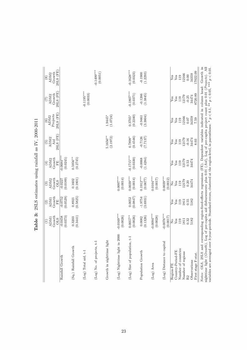
Table 3 turns to our first set of instrumental variables regressions, purging aid of its endogenous

component. In line with Bruckner (2013), we therefore regress nighttime light growth on annual

rainfall growth and its square. Columns 1 and 2 focus on ADM1 regions, excluding and including

region-fixed effects, respectively. As can be seen, the rainfall variables are completely insignif-

icant in both regressions, and therefore unsuitable as instruments in this sample. Columns 3

and 4 turn to the ADM2 level instead. Again, rainfall growth and its square are insignificant

when we do not control for region-fixed effects (in column 3). However, rainfall growth and

its square are jointly significant at the one-percent level once we include region-fixed effects (in

column 4). We find nightlight growth to decrease with rainfall growth at the one-percent level,

but to increase with its square (at the five-percent level).47 In what follows, we apply Bruckner’s

methodology to this specification only, acknowledging that the instruments lack power in our

other specifications.

Columns 5 and 6 show the corresponding second stage regressions for aid disbursements and the

number of World Bank projects, respectively. The coefficient of growth in this second stage is

then used to predict the amount of aid that is due to decreasing growth. The growth-driven part

of aid is subtracted from all aid to a particular region and period, and the resulting variable –

those parts of aid that are not endogenous to nighttime light growth – is used as an instrument

47This is contrary to the results in Bruckner (2013), who finds that growth increases with rainfall growth, butdecreases with its square.

22

Table

3:

2SL

Ses

tim

ates

usi

ng

rain

fall

asIV

,20

00-2

011

(1)

(2)

(3)

(4)

(5)

(6)

(7)

(8)

AD

M1

Gro

wth

OL

S

AD

M1

Gro

wth

FE

AD

M2

Gro

wth

OL

S

AD

M2

Gro

wth

FE

AD

M2

Aid

2S

LS

(FE

)

AD

M2

Pro

ject

s

2S

LS

(FE

)

AD

M2

Gro

wth

2S

LS

(FE

)

AD

M2

Gro

wth

2S

LS

(FE

)R

ain

fall

Gro

wth

-0.0

458

-0.0

752

-0.0

227

-0.0

684∗∗

∗

(0.0

373)

(0.0

529)

(0.0

189)

(0.0

245)

(Sq.)

Rain

fall

Gro

wth

0.3

203

0.8

921

0.1

602

0.5

956∗∗

(0.3

441)

(0.5

825)

(0.1

801)

(0.2

745)

(Log)

Tota

laid

,t-

1-0

.1195∗∗

∗

(0.0

033)

(Log)

No.

of

pro

ject

s,t-

1-0

.1499∗∗

∗

(0.0

051)

Gro

wth

inn

ightt

ime

light

5.1

656∗∗

1.9

445∗

(2.1

972)

(1.0

724)

(Log)

Nig

htt

ime

light

in2000

-0.0

169∗∗

∗0.0

097∗∗

∗

(0.0

026)

(0.0

014)

(Log)

Siz

eof

pop

ula

tion

,t-

10.0

057∗∗

0.0

052

0.0

039∗∗

∗-0

.1715∗∗

∗0.7

898∗

0.3

705∗

-0.1

807∗∗

∗-0

.1628∗∗

∗

(0.0

026)

(0.0

847)

(0.0

014)

(0.0

330)

(0.4

546)

(0.2

240)

(0.0

371)

(0.0

323)

Pop

ula

tion

Gro

wth

0.0

082

-1.9

754

0.1

912∗∗

∗-0

.0068

-0.7

126

-0.9

461

-0.1

266

-0.1

900

(0.1

326)

(3.6

931)

(0.0

677)

(1.4

284)

(7.7

137)

(3.3

804)

(1.3

845)

(1.2

293)

(Log)

Are

a-0

.0094∗∗

∗0.0

104∗∗

∗

(0.0

028)

(0.0

017)

(Log)

Dis

tan

ceto

cap

ital

-0.0

076∗∗

∗0.0

039∗∗

∗

(0.0

017)

(0.0

012)

Reg

ion

-FE

No

Yes

No

Yes

Yes

Yes

Yes

Yes

Cou

ntr

y-P

erio

d-F

EY

esY

esY

esY

esY

esY

esY

esY

esN

um

ber

of

cou

ntr

ies

119

119

119

119

119

119

119

119

Nu

mb

erof

regio

ns

1811

1811

12179

12179

12179

12166

12179

12166

R2

0.3

20.5

50.2

00.5

3-0

.16

0.0

7-0

.25

0.0

0O

bse

rvati

on

s5182

5182

34474

34474

34474

34359

34474

34359

Fir

stst

age

F-s

tat.

8.0

37.5

98720.8

917022.0

9

Notes:

OL

S,

2S

LS

an

dco

rres

pon

din

gre

gio

n-fi

xed

-eff

ects

regre

ssio

ns

(FE

).D

epen

den

tvari

ab

les

ind

icate

din

colu

mn

hea

d:

Gro

wth

inn

ightt

ime

light

(Growth

),L

og

of

per

-cap

ita

aid

dis

bu

rsem

ents

plu

s0.0

1(A

id),

Log

of

per

-cap

ita

pro

ject

cou

nt

plu

s0.0

1(P

rojects).

All

vari

ab

les

are

aver

aged

over

3-y

ear-

per

iod

s.S

tan

dard

erro

rs,

clu

ster

edat

the

regio

n-l

evel

,in

pare

nth

eses

:*p<

0.1

,**p<

0.0

5,***p<

0.0

1.

23

for total aid in the growth regressions reported in columns 7 and 8. The F-statistics on the

excluded instruments are shown at the bottom of the table. As can be seen, they are reasonably

high, but slightly below the rule-of thumb value of 10 in the aid regressions (columns 5 and 6) and

easily exceed 10 in the growth regressions (columns 7 and 8). The results of the aid effectiveness

regressions show a large and highly significant negative effect of aid on growth. The coefficients

imply that an increase in per capita aid by ten percent decreases growth by 1.1 percentage points,

while a corresponding increase in the number of projects decreases growth by 1.4 percentage

points. These effects are an order of magnitude larger compared to those above. However, due

to the strong identifying assumptions we take these results as suggestive rather than definitive.

Tables 4 and 5 turn to our preferred specification, focusing on ADM1 and ADM2 regions

respectively. Columns 1-4 replicate the main specifications of Table 1 for the greatly reduced

sample of countries that crossed the IDA-threshold at any time during our analyzed period. The

OLS results for the resulting 478 regions from 21 countries are very similar compared to Tables 1

and 2. As in the larger sample, there is no significant effect of aid on growth in ADM1 regions

(Table 1). Growth in ADM2 regions increases with aid when we do not control for region-fixed

effects, but decreases with aid otherwise (Table 2). This holds for aid disbursements and the

number of World Bank projects, the only substantive difference to the larger sample above

being that the negative correlation between project numbers and growth is now significant at

the five-percent level in the fixed effects specification.

Columns 5 and 6 show the first-stage regressions of our 2SLS approach. When we explain aid

with the interaction of the probability of receiving aid and the IDA-income threshold indicator,

we find it to be negative and highly significant in all four regressions. When we exclude region-

fixed effects (in column 5), we control for the probability of receiving aid; including region-fixed

effects (column 6), the probability of receiving aid is captured by the regional dummies. In

any case, the IDA-graduation indicator is captured by the country-period fixed effects. The F-

statistic on the excluded instrument indicates strong power. At the ADM1 level, the coefficients

of columns 5 and 6 of Table 4 imply that passing the IDA threshold reduces aid by 70 percent

when comparing a region with a probability of receiving aid of 45 percent (first quartile of the

probability’s distribution) to a region with a probability of 85 percent (third quartile). The

corresponding effect at the ADM2 level is 72 percent (Table 5).

The results for the corresponding second-stage regressions in columns 7 and 8 show that aid is

completely insignificant once its endogeneity is taken account of. This holds for the formerly

positive correlation excluding region-fixed effects for the analysis at the ADM2 level, as well

24

Table

4:

2S

LS

esti

mate

sb

ased

onth

eID

Ain

com

eth

resh

old

cros

sin

g,A

DM

1,20

00-2

012

(1)

(2)

(3)

(4)

(5)

(6)

(7)

(8)

(9)

(10)

(11)

(12)

Gro

wth

OL

SG

row

thF

EG

row

thO

LS

Gro

wth

FE

Aid

OL

SA

idF

EG

row

th2S

LS

Gro

wth

2SL

S(F

E)

Pro

ject

sO

LS

Pro

ject

sF

EG

row

th2S

LS

Gro

wth

2S

LS

(FE

)

Pr(

Aid

)*

Ab

ove

IDA

thre

shol

d-3

.051

0∗∗

∗-3

.177

3∗∗∗

-1.9

108∗∗

∗-1

.9161∗∗

∗

(0.6

232)

(0.7

065)

(0.3

913)

(0.4

268)

(Log

)T

otal

aid

,t-

1-0

.000

7-0

.003

30.

0033

0.00

28(0

.001

7)(0

.003

0)(0

.011

7)(0

.013

3)

(Log

)N

o.of

pro

ject

s,t-

10.

0002

-0.0

040

0.0

075

0.0

040

(0.0

026)

(0.0

049)

(0.0

185)

(0.0

217)

(Log

)N

ightt

ime

ligh

tin

2000

-0.0

156∗

∗∗-0

.015

7∗∗∗

0.01

01-0

.015

8∗∗

∗0.0

096

-0.0

158∗

∗∗

(0.0

036)

(0.0

037)

(0.0

471)

(0.0

036)

(0.0

373)

(0.0

036)

(Log

)S

ize

ofp

opu

lati

on,

t-1

0.00

77∗∗

-0.0

312

0.00

72∗∗

-0.0

364

0.04

421.

2615

0.00

73∗∗

-0.0

411

-0.0

203

-0.2

065

0.0

073∗∗

-0.0

365

(0.0

037)

(0.1

579)

(0.0

037)

(0.1

572)

(0.0

737)

(1.9

264)

(0.0

036)

(0.1

515)

(0.0

499)

(1.0

464)

(0.0

036)

(0.1

497)

Pop

ula

tion

Gro

wth

0.21

32-3

.202

00.

2084

-3.2

889

7.33

3870

.319

4∗∗

∗0.

1899

-3.5

401

7.9

195

22.0

263∗

0.1

485

-3.3

943

(0.3

009)

(2.1

845)

(0.3

003)

(2.1

545)

(7.4

279)

(24.

1650

)(0

.309

5)(2

.255

1)(4

.8184)

(13.0

336)

(0.3

301)

(2.1

344)

(Log

)A

rea

-0.0

055

-0.0

057

-0.0

056

-0.0

059

-0.0

251

-0.0

057

(0.0

036)

(0.0

036)

(0.0

600)

(0.0

036)

(0.0

402)

(0.0

036)

(Log

)D

ista

nce

toca

pit

al-0

.000

7-0

.000

60.

0151

-0.0

007

-0.0

008

-0.0

006

(0.0

024)

(0.0

023)

(0.0

564)

(0.0

023)

(0.0

421)

(0.0

022)

Pr(

Aid

)in

regi

onb

efor

eID

Acr

ossi

ng

5.93

29∗∗

∗-0

.015

24.0

051∗∗

∗-0

.0250

(0.1

908)

(0.0

623

)(0

.1827

)(0

.0666)

Reg

ion

-FE

No

Yes

No

Yes

No

Yes

No

Yes

No

Yes

No

Yes

Cou

ntr

y-P

erio

d-F

EY

esY

esY

esY

esY

esY

esY

esY

esY

esY

esY

esY

esN

um

ber

ofco

untr

ies

2121

2121

2121

2121

21

21

21

21

Nu

mb

erof

regi

ons

478

478

478

478

478

478

478

478

478

478

478

478

R2

0.23

0.20

0.23

0.20

0.71

0.60

0.23

0.19

0.7

70.6

30.2

20.2

0F

irst

stag

eF

-sta

t.23

.97

20.2

323.8

520.1

5O

bse

rvat

ion

s18

5818

5818

7218

7218

5818

5818

5818

5818

72

1872

1872

1872

Not

es:

OL

S,

2SL

San

dco

rres

pon

din

gre

gion

-fixed

-eff

ects

regr

essi

ons

(FE

).D

epen

den

tva

riab

les

ind

icat

edin

colu

mn

hea

d:

Gro

wth

inn

ightt

ime

light

(Gro

wth

),L

og

of

per

-cap

ita

aid

dis

bu

rsem

ents

plu

s0.

01(A

id),

Log

ofp

er-c

apit

ap

roje

ctco

unt

plu

s0.

01(P

roje

cts)

.P

r(A

id)

calc

ula

ted

asm

ean

inci

den

ceof

aid

dis

bu

rsem

ents

toa

regio

nb

efore

six

yea

rsp

ast

the

cross

ing

ofth

eID

Ain

com

eth

resh

old.

All

oth

erva

riab

les

are

aver

aged

over

3-ye

ar-p

erio

ds.

Sta

nd

ard

erro

rs,

clu

ster

edat

the

regi

on-l

evel

,in

par

enth

eses

:*p<

0.1

,**p<

0.05,

***p<

0.0

1.

25

Table

5:

2S

LS

esti

mate

sb

ased

onth

eID

Ain

com

eth

resh

old

cros

sin

g,A

DM

2,20

00-2

012

(1)

(2)

(3)

(4)

(5)

(6)

(7)

(8)

(9)

(10)

(11)

(12)

Gro

wth

OL

SG

row

thF

EG

row

thO

LS

Gro

wth

FE

Aid

OL

SA

idF

EG

row

th2S

LS

Gro

wth

2SL

S(F

E)

Pro

ject

sO

LS

Pro

ject

sF

EG

row

th2SL

SG

row

th2SL

S(F

E)

Pr(

Aid

)*

Ab

ove

IDA

thre

shol

d-0

.954

5∗∗∗

-1.4

332∗

∗∗0.1

930∗

∗-0

.3291∗

∗∗

(0.1

519)

(0.1

455)

(0.0

984

)(0

.0832)

(Log

)T

otal

aid,

t-1

0.00

09∗∗

-0.0

017∗

∗0.

001

10.

0050

(0.0

004)

(0.0

007)

(0.0

097)

(0.0

074)

(Log

)N

o.of

pro

ject

s,t-

10.

0029

∗∗∗

-0.0

032∗

∗0.0

132

0.0

103

(0.0

009)

(0.0

015)

(0.0

474)

(0.0

321)

(Log

)N

ightt

ime

ligh

tin

2000

0.01

24∗∗

∗0.

0122

∗∗∗

0.04

26∗∗

∗0.

0123

∗∗∗

0.0

388∗

∗∗0.0

117∗

∗∗

(0.0

014)

(0.0

014)

(0.0

080)

(0.0

014)

(0.0

062

)(0

.0024)

(Log

)Siz

eof

pop

ula

tion

,t-

1-0

.003

9∗∗

-0.1

039∗

∗∗-0

.003

9∗∗

-0.1

036∗∗

∗0.

0092

-1.0

583∗

∗∗-0

.004

3∗∗

∗-0

.096

5∗∗∗

-0.0

314∗∗

∗-0

.4128∗

∗∗-0

.0038∗

-0.0

979∗

∗∗

(0.0

015)

(0.0

259)

(0.0

015)

(0.0

259)

(0.0

116)

(0.2

752)

(0.0

016)

(0.0

273)

(0.0

083)

(0.1

437)

(0.0

022)

(0.0

296)

Pop

ula

tion

Gro

wth

-0.1

985∗

∗∗-0

.850

1∗∗∗

-0.2

045∗∗

∗-0

.869

8∗∗∗

-1.3

260∗

∗-0

.271

1-0

.194

8∗∗

∗-0

.845

5∗∗∗

0.5

237

0.5

518

-0.2

075∗

∗∗-0

.8759∗

∗∗

(0.0

711)

(0.2

846)

(0.0

714)

(0.2

873)

(0.6

058)

(2.0

456)

(0.0

721)

(0.2

856)

(0.3

998)

(0.9

348)

(0.0

761)

(0.2

892)

(Log

)A

rea

0.01

05∗∗

∗0.

0103

∗∗∗

0.03

69∗∗

∗0.

0102

∗∗∗

0.0

470

∗∗∗

0.0

096∗

∗∗

(0.0

018)

(0.0

018)

(0.0

117)

(0.0

018)

(0.0

088

)(0

.0029)

(Log

)D

ista

nce

toca

pit

al0.

0054

∗∗∗

0.00

54∗∗

∗0.

0739

∗∗∗

0.00

54∗∗

∗0.0

475∗

∗∗0.0

049∗

(0.0

012)

(0.0

012)

(0.0

119)

(0.0

014)

(0.0

088)

(0.0

026)

Pr(

Aid

)in

regi

onb

efor

eID

Acr

ossi

ng

6.19

26∗∗

∗0.

0086

3.0

706

∗∗∗

-0.0

254

(0.0

352)

(0.0

585)

(0.0

366)

(0.1

472)

Reg

ion-F

EN

oY

esN

oY

esN

oY

esN

oY

esN

oY

esN

oY

esC

ountr

y-P

erio

d-F

EY

esY

esY

esY

esY

esY

esY

esY

esY

esY

esY

esY

esN

um

ber

ofco

untr

ies

2121

2121

2121

2121

21

21

21

21

Num

ber

ofre

gion

s83

7583

7583

6683

6683

7583

7583

7583

758366

8366

8366

8366

R2

0.11

0.10

0.11

0.10

0.63

0.24

0.11

0.10

0.6

00.2

80.1

10.1

0F

irst

stag

eF

-sta

t.39

.48

97.0

73.8

415.6

5O

bse

rvat

ions

3197

731

977

3194

231

942

3197

731

977

3197

731

977

319

42

31942

31942

31942

Not

es:

OL

S,

2SL

San

dco

rres

pon

din

gre

gion

-fixed

-eff

ects

regr

essi

ons

(FE

).D

epen

den

tva

riab

les

indic

ated

inco

lum

nhea

d:

Gro

wth

innig

htt

ime

light

(Gro

wth

),L

og

of

per

-capit

aaid

dis

burs

emen

tsplu

s0.

01(A

id),

Log

ofp

er-c

apit

apro

ject

count

plu

s0.

01(P

roje

cts)

.P

r(A

id)

calc

ula

ted

asm

ean

inci

den

ceof

aid

dis

burs

emen

tsto

are

gion

bef

ore

six

years

past

the

cross

ing

of

the

IDA

inco

me

thre

shol

d.

All

other

vari

able

sar

eav

erag

edov

er3-

year

-per

iods.

Sta

ndar

der

rors

,cl

ust

ered

atth

ere

gion

-lev

el,

inpar

enth

eses

:*p<

0.1

,**p<

0.05,

***p<

0.0

1.

26

as the negative correlation including them. The results are very similar when we focus on the

number of World Bank projects rather than aid amounts, as shown in columns 9-12.48

In summary, our results differ tremendously across specifications. Controlling for region-fixed

effects, we do not find any significant effect of aid on growth at the ADM1 level. This holds for

the specification following Clemens et al. (2012) and according to our preferred identification

strategy. Rainfall growth and its square turned out to be weak instruments at this level so that

we did not run an aid-growth regression here. At the smaller ADM2 level, we find that growth

decreases with aid according to the fixed-effects specifications following Clemens et al. (2012) and

Bruckner (2013). Readers that are convinced of the identification strategies suggested there, and

the way we adopt them to suit our purpose of analyzing the effectiveness of aid at the regional

level, might thus conclude that aid reduces growth. However, we remain insufficiently convinced

that these strategies allow deriving causal effects of aid. Instead, we prefer to conclude in line

with the results from the regressions using our preferred identification strategy, the interaction

of the probability of receiving aid with having passed the IDA’s income threshold, that there is

no evidence that aid affects growth.

Putting these results in perspective of our expectation of a stronger link between aid and growth

at the regional level compared to the country level, our estimates are suggestive. Where we were

able to directly compare results for the regional level with results at the country level – the

analysis following Clemens et al. (2012) – we indeed find the coefficients to be significant in the

regional analysis but not at the country level. While our results for the instrumental variables

estimates are not directly comparable to results from the cross-country literature, comparing the

larger ADM1 regions to the smaller ADM2 regions indeed shows stronger correlations between

aid and growth at the ADM2 level. This suggests that analyses at smaller regional levels might

indeed lead to stronger correlations between aid from a larger number of donors than we could

consider here and (nighttime light) growth.

In what follows, we disaggregate our results according to continents and income-status, following

the United Nations’ classification as of 2014.49 Table 6 shows the results for the amount of aid

disbursed and the number of projects, following the specification of Tables 1-3. We show the

48Note however that the instrument is weak at the ADM2 level when we exclude region-fixed effects, andthe correlation of our instrument with the number of projects is positive rather than negative (see column 9 inTable 5).

49We also tested whether aid is more effective in certain policy environments than others. We do not find thisto be the case. Specifically, we interacted aid disbursements with the Polity IV indicator of democracy, the shareof people with secondary education in the population, the Fraser Index of Economic Freedom, as well as threedifferent indicators for the intensity of civil conflict, measured by the number of fatalities within a region andperiod. None of the interactions is robustly significant at conventional levels. Detailed results are available onrequest.

27

Table

6:

An

alysi

sby

conti

nen

ts,

2000

-201

2

SS

AE

CA

EA

PL

AC

ME

NA

SA

SL

DC

s

AD

M1

AD

M2

AD

M1

AD

M2

AD

M1

AD

M2

AD

M1

AD

M2

AD

M1

AD

M2

AD

M1

AD

M2

AD

M1

AD

M2

Tot

alai

dO

LS

-0.0

031

0.00

54∗∗

∗0.

0018

-0.0

012∗

∗-0

.003

4-0

.001

20.

0009

0.00

07∗∗

0.00

17-0

.001

20.0

060

0.0

003

-0.0

000

0.0

038∗

∗∗

FE

0.00

060.

0027

∗-0

.000

7-0

.003

1∗∗

∗-0

.002

1-0

.003

7∗∗

∗0.

0005

-0.0

002

0.00

290.

0031

0.0017

-0.0

020∗∗

-0.0

006

0.0

012

2SL

S0.

0390

∗∗∗

-0.0

034∗∗

∗0.

0312

∗∗∗

0.01

49∗∗

∗-0

.030

2∗∗∗

-0.1

036∗∗

∗0.

0220

∗∗∗

0.07

93∗∗

∗-0

.005

5∗∗∗

0.00

26∗∗

-0.0

281∗

∗∗0.0

501∗

∗∗0.6

077∗

∗∗0.0

500∗

∗∗

F-s

tat.

(0.3

1)(1

.94)

(6.2

7)(1

4.36

)(0

.30)

(3.0

3)(0

.74)

(0.1

7)(1

.38)

(0.9

9)(1

.38)

(2.5

7)

(0.0

0)

(3.4

9)

2SL

S(F

E)

0.01

84∗∗

∗0.

0239

∗∗∗

0.02

08∗∗

∗0.

0015

∗0.

3851

∗∗∗

-0.0

867∗∗

∗0.

0501

∗∗∗

0.14

74∗∗

∗0.

0367

∗∗∗

-0.2

895∗∗

∗0.0

225∗

∗∗-0

.0372∗

∗∗0.0

379∗

∗∗0.2

879∗

∗∗

F-s

tat.

(0.5

2)(1

.25)

(9.7

7)(2

5.36

)(0

.07)

(3.7

7)(0

.25)

(0.6

3)(1

.17)

(0.5

8)(3

.20)

(5.4

2)

(1.4

1)

(0.7

1)

Nu

mb

erof

cou

ntr

ies

4242

2828

1515

2929

1010

88

41

41

Nu

mb

erof

regi

ons

534

6191

594

8184

277

1369

647

117

865

205

3823

142

4408

540

6167

Ob

serv

atio

ns

1998

1957

823

1931

132

1031

4691

018

4567

404

817

1474

6531

16116

1955

18612

SS

AE

CA

EA

PL

AC

ME

NA

SA

SL

DC

s

AD

M1

AD

M2

AD

M1

AD

M2

AD

M1

AD

M2

AD

M1

AD

M2

AD

M1

AD

M2

AD

M1

AD

M2

AD

M1

AD

M2

Pro

ject

sO

LS

-0.0

047

0.00

83∗∗

∗0.

0033

∗-0

.000

9-0

.008

4∗

-0.0

019

0.00

210.

0015

∗∗∗

0.00

22-0

.002

00.0

056

0.0

019

-0.0

001

0.0

075∗

∗∗

FE

0.00

510.

0045

∗-0

.001

7-0

.002

9∗∗

-0.0

025

-0.0

061∗∗

∗0.

0017

-0.0

003

0.00

490.

0049

∗∗-0

.0050

-0.0

028

0.0

022

0.0

063∗

∗∗

2SL

S0.

1033

∗∗∗

-0.0

824∗∗

∗0.

0437

∗∗∗

0.01

12∗∗

∗-0

.130

2∗∗∗

0.07

00∗∗

∗0.

0346

∗∗∗

-0.4

370∗

∗∗-0

.033

8∗∗∗

0.10

34∗∗

∗-0

.0221∗

∗∗0.1

157∗

∗∗1.8

913∗

∗∗0.0

460∗

∗∗

F-s

tat.

(0.3

1)(1

.88)

(6.1

5)(1

4.93

)(0

.30)

(2.7

3)(0

.74)

(0.2

8)(1

.29)

(0.9

2)(1

.38)

(2.3

7)

(0.0

0)

(3.3

1)

2SL

S(F

E)

-0.1

090∗∗

∗0.

1570

∗∗∗

0.01

84∗∗

∗0.

0147

∗∗∗

0.07

62∗∗

∗0.

1119

∗∗∗

-0.1

653∗∗

∗-0

.034

2∗∗∗

0.07

73∗∗

∗-0

.114

1∗∗

∗0.

0008

-0.0

750∗

∗∗-0

.0170∗

∗0.3

892∗

∗∗

F-s

tat.

(0.5

2)(1

.11)

(9.9

8)(2

4.83

)(0

.07)

(3.9

1)(0

.25)

(0.6

2)(1

.19)

(0.4

1)(3

.20)

(4.9

0)

(1.4

1)

(0.8

3)

Nu

mb

erof

cou

ntr

ies

4242

2827

1515

2929

1010

88

41

41

Nu

mb

erof

regi

ons

534

6185

594

8165

276

1368

746

517

846

205

3817

142

4405

540

6146

Ob

serv

atio

ns

1996

1963

923

3830

947

1018

4692

518

1667

507

820

1465

1531

16134

1951

18532

Not

es:

Sh

ows

the

coeffi

cien

tsof

the

resp

ecti

veai

dva

riab

le.

OL

S,

2SL

San

dco

rres

pon

din

gre

gion

-fixed

-eff

ects

regr

essi

ons

(FE

).D

epen

den

tva

riab

le:

Gro

wth

inn

ightt

ime

light.

Th

ere

gre

ssio

ns

incl

ud

eco

untr

y-p

erio

dfi

xed

-eff

ects

and

,if

FE

issp

ecifi

ed,

also

regi

on-fi

xed

effec

ts.

Log

ged

nig

htt

ime

ligh

tin

2000

,lo

gged

pop

ula

tion

size

,p

opu

lati

on

gro

wth

,lo

gged

are

a,

an

dlo

gged

dis

tan

ceto

cap

ital

are

incl

ud

edas

contr

olva

riab

les

inth

eO

LS

and

2SL

Sre

gres

sion

s.A

llva

riab

les

are

aver

aged

over

3-ye

ar-p

erio

ds.

F-s

tati

stic

sre

fer

toth

eco

rres

pond

ing

firs

tst

age.

Sta

nd

ard

erro

rs,

clu

ster

edat

the

regi

on-l

evel

,in

par

enth

eses

:*p<

0.1,

**p<

0.0

5,**

*p<

0.0

1.S

SA

:S

ub

-Sah

aran

Afr

ica;

EC

A:

Eu

rop

ean

dC

entr

alA

sia;

EA

P:

Eas

tA

sia

and

Pac

ific;

LA

C:

Lat

inA

mer

ica

and

Car

rib

ean

;M

EN

A:

Mid

dle

East

an

dN

ort

her

nA

fric

a;

SA

S:

Sou

thA

sia;

LD

Cs:

Lea

st-d

evel

oped

cou

ntr

ies.

28

resulting coefficient of aid disbursements or project numbers and indicate whether the coefficient

is statistically significant. For the 2SLS regressions we include the first-stage F-statistics in

parentheses. We do not separate the sample using our preferred instrument – the interaction of

crossing the IDA-threshold with the probability to receive aid – given that the resulting number

of countries and regions would be too low for meaningful regressions.

The results show some differences across continents. Focusing on the region-fixed effects speci-

fications without using instruments, there is no significant correlation between aid and growth

at the ADM1 level. At the ADM2 level, growth increases with aid in Sub-Saharan Africa, but

decreases with aid in Europe and Central Asia, East Asia and Pacific, and South Asia. If we

focus on the least developed countries only, there is no significant correlation between aid and

growth. Turning to the 2SLS regressions employing rainfall growth and its square as instruments,

the first-stage F-statistic exceeds 10 only in the regressions restricted to Europe and Central

Asia. Contrary to the results with OLS, these regressions show that growth increases with aid.

The lower panel of Table 6 shows results corresponding to the number of projects. Overall,

these results are very similar, with the exception of an insignificant coefficient for South Asia in

the fixed effects regression at the ADM2 level and a significant and positive correlation between

projects and growth in this specification in least developed countries. Overall, while not showing

strong evidence of a positive causal effect of aid and growth, these results imply that the effects

of aid on growth are likely to be heterogeneous across groups of countries. Unfortunately, rainfall

growth and its square turned out to be weak in most specifications, so that these coefficients

hardly show more than interesting correlations however. We thus leave a deeper analysis of

heterogeneous effects of aid for future research.

4 Conclusion

The aim of this paper was to bring the aid effectiveness debate to the regional level. We

hypothesized that the effects of aid might be discernible regionally, even if aid amounts are

too low to be measurable at the country level. The lack of sub-regional analyses might thus

contribute to the lack of robust evidence in the aid effectiveness literature.

Our regressions used geo-coded data for World Bank aid to a maximum of 2,283 regions

in 130 countries over the 2000-2011 period, testing whether and to what extent aid affects

development, measured as nighttime light growth. We presented results using three different

identification strategies. First, we followed Clemens et al. (2012), relying on aid that can

29

reasonably be expected to affect growth in the short run, controlling for country- and region-fixed

effects, and lagging aid appropriately to allow time for it to become effective. Second, we purge

aid of those parts that are endogenous to growth, using data on rainfall growth and its square

in the spirit of Bruckner (2013). However, our instruments are too weak to allow us to draw

any strong conclusions.

Our preferred identification strategy exploited variation arising from interacting a variable that

indicates whether or not a country crossed the IDA’s income threshold for concessional aid

with a recipient region’s probability of receiving aid. This comes with the disadvantage that

the analysis only includes those countries that crossed the IDA threshold during the time our

sample covers. Controlling for the levels of the interacted variables, the interaction provides a

powerful and excludable instrument for a sample of 478 regions from 21 countries.

Overall, our results show significant correlations between aid and (nighttime light) growth.

Our results highlight the importance of measuring aid flows at the regional level, showing

correlations that are markedly stronger at the smaller ADM2 regional level, compared to the

larger ADM1 and the country level. However, once we take account of the endogeneity of aid –

and potential attenuation bias, e.g., through measurement error in the geo-coding process – we

find no significant effect of World Bank aid on growth, neither at the ADM1 nor the ADM2 level.

While the World Bank is one of the world’s largest donors, the amounts of aid we could track here

only represent a share of all World Bank project aid, and are of course comparably small when

put in perspective to aid amounts included in most aid effectiveness studies at the country level

(usually using aid from all major Western donors). One reason for the insignificant result might

thus be that the amounts of (region-specific) World Bank aid alone are too low to measurably

affect growth, even at the regional level. Our failure to detect a significant effect of aid on

growth is likely to be aggravated by the potential fungibility of aid.50 To the extent that aid is

fungible, the aid might have positive growth effects in other regions that we fail to measure with

our analysis. The same might hold if regional spillovers are important. Of course, this would

not threaten our conclusion regarding the effect of aid on growth in the regions that receive the

aid.

It is important to emphasize that these results not necessarily hold for aid more broadly.

First, our analysis is limited to countries that passed the IDA-income threshold at some time

50Fungibility is likely to be partial rather than full (van de Sijpe, 2013). Van de Walle and Mu (2007) findevidence of a “flypaper effect” rather than full fungibility in their study of a road rehabilitation project co-financedby the World Bank in Vietnam.

30

during our sample period, giving rise to the question of external validity. As Galiani et al.

(2014) show, countries crossing the IDA income threshold do not display systematically different

growth patterns than countries below the income threshold, controlled for initial income. They

consequently expect their estimated effect of aid on growth to hold in a broader set of countries

rather than being limited to countries that passed the threshold. The same will arguably be

true for the results of our study. Second, the focus of our study was on project aid that could be

attributed to specific regions with sufficient precision. Other forms of aid – like budget support

to the central government, for example – are not covered here, and might differ in their impact.

And third, the results for the World Bank do not necessarily translate to other donors also.51

Analyzing the effect of aid on growth at the regional level for a broader set of donors is currently

prevented by the unavailability of aid data on the regional level. Other than for the World

Bank, current data availability would allow a similar analysis for Chinese aid in Africa, where

geo-coded data for a similar period of time as we have used here has recently been made available

(Dreher et al., 2014). More broadly, another promising extension includes the analysis of the

effects of aid on broader indicators of social development than growth at the subnational level,

which is equally missing from the current literature. Geo-coding aid flows for a larger number

of donors across the world remains a challenge for future research on the effectiveness of aid.

51Note however that Rajan and Subramanian (2008) do not find differential effects of budget compared toproject aid on growth at the country level. The same holds for bilateral compared to multilateral aid.

31

References

Ahmed, F. Z. (2013). The Impact of US Economic Aid on Political Rights. Working Paper,

Oxford University.

AidData (2015). Geocoded data from the world bank ibrd-ida, version 1.0. http://aiddata.

org.

Bazzi, S. and Clemens, M. A. (2013). Blunt Instruments: Avoiding Common Pitfalls in

Identifying the Causes of Economic Growth. American Economic Journal: Macroeconomics,

5(2):152–186.

Bhandari, L. and Roychowdhury, K. (2011). Night Lights and Economic Activity in India:

A Study Using DMSP-OLS Night Time Images. Proceedings of the Asia-Pacific Advanced

Network, 32:218–236.

Bjørnskov, C. (2013). Types of Foreign Aid. Working Paper, School of Economics and

Management, University of Aarhus.

Boockmann, B. and Dreher, A. (2003). The Contribution of the IMF and the World Bank to

Economic Freedom. European Journal of Political Economy, 19(3):633–649.

Bruckner, M. (2013). On the Simultaneity Problem in the Aid and Growth Debate. Journal of

Applied Econometrics, 28(1):126–150.

Chauvet, L. and Ehrhart, H. (2014). Aid and Growth–Evidence from Firm-level Data. Paper

presented at the German Research Committee Development Economics 2014 Conference.

Chen, X. and Nordhaus, W. D. (2011). Using Luminosity Data as a Proxy for Economic

Statistics. Proceedings of the National Academy of Sciences, 108(21):8589–8594.

CIESIN (2005). Gridded population of the world, version 3, center for international earth science

information network - columbia university, united nations food and agricultural programme,

and centro internactional de agricultura tropical.

Clemens, M. A., Radelet, S., Bhavnani, R. R., and Bazzi, S. (2012). Counting Chickens when

They Hatch: Timing and the Effects of Aid on Growth. Economic Journal, 122(561):590–617.

Dionne, K. Y., Kramon, E., and Roberts, T. (2013). Aid Effectiveness and Allocation: Evidence

from Malawi. Paper Presentation, ASA 2013 Annual Meeting.

32

http://aiddata.org

http://aiddata.org

Doll, C., M. J.-P. and Morley, J. (2006). Mapping Regional Economic Activity From Night-Time

Light Satellite Imagery. Ecological Economics, 57(1):75–92.

Doucouliagos, H. and Paldam, M. (2009). The Aid Effectiveness Literature: The Sad Results

Of 40 Years Of Research. Journal of Economic Surveys, 23(3):433–461.

Dreher, A., Fuchs, A., Hodler, R., Parks, B., Raschky, P. A., and Tierney, M. J. (2014). Aid

on Demand: African Leaders and the Geography of China’s Foreign Assistance. AidData

Working Paper No. 3, AidData.

Dreher, A., Klasen, S., Vreeland, J. R., and Werker, E. (2013). The Costs of Favoritism:

Is Politically Driven Aid Less Effective? Economic Development and Cultural Change,

62(1):157–191.

Dreher, A. and Langlotz, S. (2015). Aid and Growth: New Evidence Using an Excludable

Instrument. Mimeo, University of Heidelberg.

Easterly, W. and Kraay, A. (2000). Small States, Small Problems? Income, Growth, and

Volatility in Small States. World Development, 28(11):2013–2027.

Elvidge, C. D., Baugh, K. E., Kihn, E. A., Kroehl, H. W., and Davis, E. R. (1997). Mapping City

Lights with Nighttime Data from the DMSP Operational Linescan System. Photogrammetric

Engineering and Remote Sensing, 63(6):727–734.

Elvidge, C. D., Hsu, F.-C., Baugh, K. E., and Ghosh, T. (2014). National Trends in Satellite-

Observed Lighting: 1992–2012. In Weng, Q., editor, Global Urban Monitoring and Assessment

Through Earth Observation, pages 97–118. CRC Press.

Findley, M. G., Powell, J., Strandow, D., and Tanner, J. (2011). The Localized Geography of

Foreign Aid: A New Dataset and Application to Violent Armed Conflict. World Development,

39(11):1995–2009.

Galiani, S., Knack, S., Xu, L. C., and Zou, B. (2014). The Effect of Aid on Growth: Evidence

From a Quasi-Experiment. World Bank Policy Research Paper No. 6865, Washington DC.

Henderson, J. V., Storeygard, A., and Weil, D. N. (2012). Measuring Economic Growth from

Outer Space. American Economic Review, 102(2):994–1028.

Hodler, R. and Raschky, P. A. (2014). Regional Favoritism. The Quarterly Journal of Economics,

129(2):995–1033.

33

Jablonski, R. S. (2014). How Aid Targets Votes: The Impact of Electoral Incentives on Foreign

Aid Distribution. World Politics, 66(2):293–330.

Jerven, M. (2013). Poor Numbers: How We Are Misled by African Development Statistics and

What to Do About It. Cornell University Press, New York.

Kerner, A., Beatty, A., and Jerven, M. (2014). Real Money, Fake Data: The Political Economy

of World Bank Data Manipulation. Working Paper, University of Michigan.

Knack, S., Xu, L. C., and Zou, B. (2014). Interactions Among Donors’ Aid Allocations: Evidence

From an Exogenous World Bank Income Threshold. World Bank Policy Research Paper No.

7039, Washington DC.

Michalopoulos, S. and Papaioannou, E. (2013). Pre-Colonial Ethnic Institutions and

Contemporary African Development. Econometrica, 81(1):113–152.

Michalopoulos, S. and Papaioannou, E. (2014). National Institutions and Subnational

Development in Africa. The Quarterly Journal of Economics, 129(1):151–213.

Mosley, P. (1987). Foreign Aid, its Defense and Reform. University Press of Kentucky,

Lexington, KY.

Mveyange, A. (2015). Night Lights and Regional Income Inequality in Africa. Technical report,

University of Southern Denmark.

NOAA (n.d.). Version 4 dmsp-ols nighttime lights time series, national oceanic and atmospheric

administration, boulder: National geophysical data center.

Noor, A. M., Alegana, V. A., Gething, P. W., Tatem, A. J., Snow, R. W., et al. (2008). Using

Remotely Sensed Night-Time Light as a Proxy for Poverty in Africa. Population Health

Metrics, 6(5).

Nunn, N. and Qian, N. (2014). US Food Aid and Civil Conflict. American Economic Review,

104(6):1630–1666.

Nunnenkamp, P., Ohler, H., and Andres, M. S. (2012). Need, Merit, and Politics in Multilateral

Aid Allocation: A District-Level Analysis of World Bank Projects in India. Working Paper

No. 1783, Kiel Institute for the World Economy.

Ohler, H. (2013). Do Aid Donors Coordinate within Recipient Countries? Department of

Economic Discussion Paper No. 539, University of Heidelberg.

34

Ohler, H. and Nunnenkamp, P. (2014). Needs-Based Targeting or Favoritism? The Regional

Allocation of Multilateral Aid within Recipient Countries. Kyklos, 67(3):420–446.

Olivia, S., G. J.-B. L. and Stichbury, G. (2015). Monitoring Economic Activity in Indonesia

using Night Light Detected from Space. Technical report, Monash University.

Peratsakis, C., Powell, J., Findley, M., Baker, J., and Weaver, C. (2012). Geocoded Activity-level

Data from the Government of Malawi’s Aid Management Platform. Working Paper, AidData

and the Robert S. Strauss Center for International Security and Law.

Powell, J. and Findley, M. G. (2012). The Swarm Principle? A Sub-national Spatial Analysis

of Donor Coordination in Sub-Saharan Africa. Mimeo, mimeo.

Rajan, R. G. and Subramanian, A. (2008). Aid and Growth: What Does the Cross-Country

Evidence Really Show? The Review of Economics and Statistics, 90(4):643–665.

Rajlakshmi, D. (2013). Foreign Aid Allocation and Impact: A Sub-National Analysis of Malawi.

Dissertation, Duke University.

Roodman, D. (2015). A Replication of “Counting Chickens when They Hatch” (Economic

Journal 2012). Public Finance Review, 43(2):256–281.

Schneider, U., Becker, A., Finger, P., Meyer-Christoffer, A., Rudolf, B., and Ziese, M. (2011).

GPCC Full Data Reanalysis Version 6.0 at 0.5◦: Monthly Land-Surface Precipitation from

Rain-Gauges built on GTS-based and Historic Data.

Strandow, D., Findley, M., Nielson, D., and Powell, J. (2011). The UCDP-AidData Codebook on

Geo-Referencing Foreign Aid. Version 1.1. Uppsala Conflict Data Program, Uppsala, Sweden.

Sutton, P. C. and Costanza, R. (2002). Global Estimates of Market and Non-market Values

Derived From Nighttime Satellite Imagery, Land Cover, and Ecosystem Service Valuation.

Ecological Economics, 41(3):509–527.

van de Sijpe, N. (2013). Is Foreign Aid Fungible? Evidence from the Education and Health

Sectors. World Bank Economic Review, 27(2):320–356.

van de Walle, D. and Mu, R. (2007). Fungibility and the Flypaper Effect of Project Aid:

Micro-Evidence for Vietnam. Journal of Development Economics, 84(2):667–685.

Werker, E., Ahmed, F. Z., and Cohen, C. (2009). How Is Foreign Aid Spent? Evidence from a

Natural Experiment. American Economic Journal: Macroeconomics, 1(2):225–244.

35

Zhang, G. (2004). The Determinants of Foreign Aid Allocation Across China: The Case of

World Bank Loans. Asian Survey, 44(5):691–710.

36

Appendix

37

Table

A.1:

Des

crip

tion

ofke

yva

riab

les

Variable

Source

Desc

rip

tion

Nig

htt

ime

light

inte

nsi

tyN

OA

AS

um

of

nig

htt

ime

light

inte

nsi

tyvalu

esfa

llin

gw

ith

inth

eb

ord

ers

of

an

ad

min

istr

ati

ve

regio

n

Tota

laid

(p.c

.)A

idD

ata

(2015)

/W

orl

dB

an

kA

ver

age

an

nu

al

dis

bu

rsem

ent

thro

ugh

Worl

dB

an

kp

roje

cts

wit

hin

are

gio

nd

ivid

edby

regio

nal

pop

ula

tion

,2011

US

$

Earl

y-i

mp

act

aid

(p.c

.)A

idD

ata

(2015)

/C

lem

ens

etal.

(2012)

Su

bco

mp

on

ent

of

“T

ota

laid

”fr

om

pro

ject

sin

earl

y-i

mp

act

sect

ors

,cl

ass

ified

on

the

basi

sof

Cle

men

set

al.

(2012)

Late

-im

pact

aid

(p.c

.)A

idD

ata

(2015)

/C

lem

ens

etal.

(2012)

Su

bco

mp

onen

tof

“T

ota

laid

”fr

om

pro

ject

sin

late

-im

pact

sect

ors

,cl

ass

ified

on

the

basi

sof

Cle

men

set

al.

(2012)

No.

of

pro

ject

s(p

.c.)

Aid

Data

(2015)

Aver

age

an

nu

al

nu

mb

erof

pro

ject

wit

hn

on

-zer

od

isb

urs

emen

tsw

ith

ina

regio

nd

ivid

edby

regio

nal

pop

ula

tion

Siz

eof

pop

ula

tion

CIE

SIN

(2005)

Est

imate

dh

ead

cou

nt

of

pop

ula

tion

base

don

sate

llit

eim

age

gau

ges

of

pop

ula

tion

den

sity

Are

aG

lob

al

Ad

min

istr

ati

ve

Are

as

(GA

DM

)S

ize

of

the

ad

min

istr

ati

ve

regio

n,

squ

are

met

res

Dis

tan

ceto

cap

ital

Glo

bal

Ad

min

istr

ati

ve

Are

as

(GA

DM

)S

hort

est

dis

tan

ceb

etw

een

the

centr

eof

an

ad

min

istr

ati

ve

regio

nan

dth

eco

untr

yca

pit

al,

kilom

etre

s

An

nu

al

rain

fall

Sch

nei

der

etal.

(2011)

Aver

age

an

nu

al

rain

fall

esti

mate

dfr

om

the

sum

of

rain

fall

inte

nsi

tyvalu

esfa

llin

gw

ith

inth

eb

ord

ers

of

are

gio

n

Ab

ove

IDA

thre

shold

base

don

Kn

ack

etal.

(2014)

Bin

ary

ind

icato

rta

kin

gvalu

e1

ifa

cou

ntr

yis

six

yea

rsp

ast

the

cross

ing

of

the

IDA

inco

me

thre

shold

Pr(

Aid

)ow

nca

lcu

lati

on

sM

ean

inci

den

ceof

aid

dis

bu

rsem

ents

toa

regio

nb

efore

six

yea

rsp

ast

the

cross

ing

of

the

IDA

inco

me

thre

shold

NO

AA

:N

ati

on

al

Oce

an

ican

dA

tmosp

her

icA

dm

inis

trati

on

.

CIE

SIN

:C

ente

rfo

rIn

tern

ati

on

al

Eart

hS

cien

ceIn

form

ati

on

Net

work

.

38

Table A.2: Descriptive Statistics, ADM1, Estimation sample (2000-2012)

Mean Median SD Min. Max.

Nighttime light intensity 2.45 0.60 5.89 0.00 63.00

Growth in nighttime light 0.06 0.04 0.12 -0.33 0.62

Size of population, t-1 (in 1,000) 2361.73 498.43 9115.85 0.79 189844.11

Area (in million square km) 41037.08 7396.56 122254.88 17.38 3066310.00

Distance to capital (in km) 403.97 227.15 643.78 0.61 11212.19

Total aid, t-1 (per capita) 2.39 0.60 4.43 0.00 37.65

Early-impact aid, t-1 (per capita) 1.20 0.00 2.75 0.00 22.56

Late-impact aid, t-1 (per capita) 0.99 0.07 1.95 0.00 18.02

No. of projects, t-1 (per 1,000 capita) 0.00 0.00 0.00 0.00 0.01

No. of early-impact projects, t-1 (per 1,000 capita) 0.00 0.00 0.00 0.00 0.00

No. of late-impact projects, t-1 (per 1,000 capita) 0.00 0.00 0.00 0.00 0.01

Rainfall Growth 0.01 0.01 0.06 -0.15 0.21

Pr(Aid) in region before IDA crossing 0.62 0.70 0.31 0.00 1.00

Observations 9124

Number of countries 130

Number of regions 2281

Table A.3: Specification at country-level, 2000-2012

(1) (2) (3) (4)

(Log) Total aid, t-1 -0.0006

(0.0022)

(Log) No. of projects, t-1 -0.0010

(0.0024)

(Log) Early-impact aid, t-1 0.0020

(0.0020)

(Log) Late-impact aid, t-1 -0.0003

(0.0020)

(Log) No. of early-impact projects, t-1 0.0010

(0.0019)

(Log) No. of late-impact projects, t-1 0.0003

(0.0027)

(Log) Size of population, t-1 -0.0079 -0.0079 -0.0179 -0.0123

(0.0967) (0.0970) (0.0975) (0.0970)

Country-FE Yes Yes Yes Yes

Period-FE Yes Yes Yes Yes

Number of countries 130 130 130 130

R2 0.22 0.22 0.22 0.22

Observations 1529 1529 1529 1529

Notes: Within-country regressions (FE). Dependent variable: Growth in nighttime light.All variables are averaged over 3-year-periods. Standard errors, clustered at the country-level, in parentheses: * p < 0.1, ** p < 0.05, *** p < 0.01.

39

Aid and Growth at the Regional Level; by Axel Dreher and ... · ADM2 regions from 21 countries....

Documents

Transcript of Aid and Growth at the Regional Level; by Axel Dreher and ... · ADM2 regions from 21 countries....