AGRICULTURE WATER DEMAND MODEL · 2018-03-12 · AGRICULTURE WATER DEMAND MODEL Report for Salt...
46
AGRICULTURE WATER DEMAND MODEL Report for Salt Spring Island December 2017 Photo Credit: Shannon Cowan
Transcript of AGRICULTURE WATER DEMAND MODEL · 2018-03-12 · AGRICULTURE WATER DEMAND MODEL Report for Salt...
AGRICULTURE WATER DEMAND MODEL
Report for Salt Spring Island
December 2017
Photo Credit: Shannon Cowan

AGRICULTURE WATER DEMAND MODEL
Report for Salt Spring Island
December 2017
Authors: Stephanie Tam, P.Eng. Water Management Engineer B.C. Ministry of Agriculture Innovation and Adaption Services Branch Abbotsford, BC
Ted van der Gulik, P.Eng. President Partnership for Water Sustainability in BC Abbotsford, BC
This project is funded in part through Growing Forward 2, a federal-provincial-territorial initiative.
DISCLAIMER The data that is presented in this report provides the best estimates for agriculture water demand that can be generated at this time. While every effort has been made to ensure the accuracy and completeness of the information, the information should not be considered as final. The Governments of Canada and British Columbia are committed to working with industry partners. Opinions expressed in this document are those of the authors and not necessarily those of the Governments of Canada and British Columbia or other funding partners identified above.

Agriculture Water Demand Model – Report for Salt Spring Island December 2017 2
Agriculture Water Demand Model – Report for Salt Spring Island December 2017 3
Table of Contents
Table of Contents .................................................................................................................... 3
Acknowledgements ................................................................................................................. 5
Background .............................................................................................................................. 6
Methodology ............................................................................................................................ 7
Cadastre .......................................................................................................................................................... 8
Land Use Survey ............................................................................................................................................. 8
Soil Information ............................................................................................................................................. 10
Climate Information ....................................................................................................................................... 11
Model Calculations ................................................................................................................ 12
Crop .............................................................................................................................................................. 12
Irrigation ........................................................................................................................................................ 12
Soil ................................................................................................................................................................ 12
Climate .......................................................................................................................................................... 13
Agricultural Water Demand Equation ............................................................................................................ 13
Livestock Water Use .............................................................................................................. 18
Definition and Calculation of Individual Terms Used in the Irrigation Water Demand Equation ................................................................................................................................. 19
Growing Season Boundaries ......................................................................................................................... 19
Evapotranspiration (ETo) ............................................................................................................................... 21
Availability Coefficient (AC) ........................................................................................................................... 21
Rooting Depth (RD) ....................................................................................................................................... 21
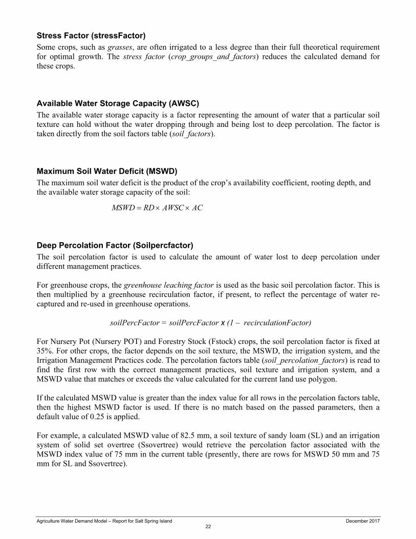
Stress Factor (stressFactor) .......................................................................................................................... 22
Available Water Storage Capacity (AWSC) ................................................................................................... 22
Maximum Soil Water Deficit (MSWD) ............................................................................................................ 22
Deep Percolation Factor (Soilpercfactor) ...................................................................................................... 22
Maximum Evaporation Factor (maxEvaporation) .......................................................................................... 23
Irrigation Efficiency (Ie) .................................................................................................................................. 23
Soil Water Factor (swFactor) ......................................................................................................................... 23
Early Season Evaporation Factor (earlyEvaporationFactor) ......................................................................... 23
Crop Coefficient (Kc) ...................................................................................................................................... 23
Growing Degree Days (GDD) ........................................................................................................................ 24
Frost Indices .................................................................................................................................................. 24
Corn Heat Units (CHU) .................................................................................................................................. 24
Corn Season Start and End ........................................................................................................................... 25
Tsum Indices ................................................................................................................................................. 25
Wet/Dry Climate Assessment ........................................................................................................................ 25
Groundwater Use .......................................................................................................................................... 25
Agriculture Water Demand Model – Report for Salt Spring Island December 2017 4
Land Use Results................................................................................................................... 26
Agricultural Water Demand Results ..................................................................................... 28
Annual Crop Water Demand – Tables A and B ............................................................................................. 28
Annual Water Demand by Irrigation System – Table C ................................................................................. 28
Annual Water Demand by Soil Texture – Table D ......................................................................................... 28
Annual Water Demand by Aquifer – Table E ................................................................................................. 28
Irrigation Management Factors – Table F ..................................................................................................... 28
Deep Percolation – Table G .......................................................................................................................... 30
Improved Irrigation Efficiency and Good Management – Table H ................................................................. 30
Livestock Water Use – Table I ....................................................................................................................... 30
Climate Change Water Demand for 2050 – Table J ...................................................................................... 30
Agricultural Buildout Crop Water Demand Using 2003 Climate Data – Table K ............................................ 32
Agricultural Buildout Crop Water Demand for 2050 – Table L ....................................................................... 33
Irrigation Systems Used for the Buildout Scenario for 2003 – Table M ......................................................... 34
Water Demand for the Buildout Area by Aquifer 2003 Climate Data – Table N............................................. 34
Literature ................................................................................................................................ 35
Appendix Tables .................................................................................................................... 36
List of Figures Figure 1 Map of Salt Spring Island (SSI) .................................................................................................... 6 Figure 2 Map of the Project Area Overlaid with Map Sheets ...................................................................... 7 Figure 3 Land Use Survey .......................................................................................................................... 8 Figure 4 GIS Map Sheet ............................................................................................................................. 9 Figure 5 Cadastre with Polygons ................................................................................................................ 9 Figure 6 GIS Model Graphics ................................................................................................................... 10 Figure 7 Climate Stations in the Project Area ........................................................................................... 11 Figure 8 Water Areas in the Project Area ................................................................................................. 27 Figure 9 Land Parcels in the Project Area ................................................................................................ 27 Figure 10 Annual ET and Effective Precipation in 2050's ........................................................................... 31 Figure 11 Future Irrigation Demand for All Outdoor Uses in the Okanagan in Response to Observed
Climate Data (Actuals) and Future Climate Data Projected from a Range of Global Climate Models ....................................................................................................................................... 32
Figure 12 Irrigation Expansion Potential for the Project Area ..................................................................... 33
List of Tables Table 1 Livestock Water Demand (Litres/day) ........................................................................................ 18 Table 2 Overview of the Land and Inventoried Area .............................................................................. 26 Table 3 Summary of Primary Agricultural Activities within the ALR where Primary Land Use is
agriculture in the Project Area ................................................................................................. 26 Table 4 Irrigation Management Factors .................................................................................................. 29
Agriculture Water Demand Model – Report for Salt Spring Island December 2017 5
Acknowledgements The Ministry of Agriculture acknowledges the work done by:
Ron Fretwell Program Developer RHF Systems Ltd.
Denise Neilsen Research Scientist Summerland Research and Development Centre Agriculture and Agri-Food Canada
in the original development of the model algorithms, climate change scenarios and model development. Without their effort, the development of the model would not have been possible. There are over twenty people that have been involved with the preparation and collection of data for the development of the Agriculture Water Demand Model in the project area. The authors wish to express appreciation to the following individuals for their contribution for the tasks noted. Alex Cannon Environment and Climate Change Canada Climate data downscaling Bill Taylor Environment and Climate Change Canada Climate data layer Corrine Roesler Ministry of Agriculture GIS data coordination Sam Lee Ministry of Agriculture GIS data preparation Derek Masselink Ministry of Agriculture Land Use Inventory Michael Dykes Contractor Land Use Inventory

Agriculture Water Demand Model – Report for Salt Spring Island December 2017 6
Background The Agriculture Water Demand Model (AWDM) was developed in the Okanagan Watershed. It was developed in response to rapid population growth, drought conditions from climate change, and the overall increased demand for water. Many of the watersheds in British Columbia (BC) are fully allocated already or may be in the next 15 to 20 years. The AWDM helps to understand current agricultural water use and helps to fulfil the Province’s commitment under the “Living Water Smart – BC Water Plan” to reserve water for agricultural lands. The Model can be used to establish agricultural water reserves throughout the various watersheds in BC by providing current and future agricultural water use data. Climate change scenarios developed by the University of British Columbia (UBC) and the Summerland Research and Development Centre predict an increase in agricultural water demand due to warmer and longer summers and lower precipitation during summer months in the future. The Model was developed to provide current and future agricultural water demands. The Model calculates water use on a property-by-property basis, and sums each property to obtain a total water demand for the entire basin or each sub-basin. Crop, irrigation system type, soil texture and climate data are used to calculate the water demand. Climate data from 2003 was used to present information on one of the hottest and driest years on record, and 1997 data was used to represent a wet year. Lands within the Agriculture Land Reserve (ALR), depicted in green in Figure 1, were included in the project.
Figure 1 Map of Salt Spring Island (SSI)

Agriculture Water Demand Model – Report for Salt Spring Island December 2017 7
Methodology The Model is based on a Geographic Information System (GIS) database that contains information on cropping, irrigation system type, soil texture and climate. An explanation of how the information was compiled for each is given below. The survey area included all properties within the ALR and areas that were zoned for agriculture by the local governments. The inventory was undertaken by Ministry of Agriculture (AGRI) staff, hired professional contractors and summer students.
Figure 2 Map of the Project Area Overlaid with Map Sheets

Agriculture Water Demand Model – Report for Salt Spring Island December 2017 8
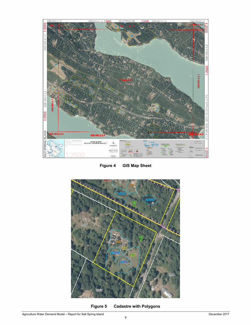
Cadastre Cadastre information was provided by the Integrated Cadastral Information Society (ICIS). A consultant was hired to unify all of the cadastral information into one seamless cover for the entire watershed. This process allows the Model to calculate water demand for each parcel and to report out on sub-basins, local governments, water purveyors or groundwater aquifers by summing the data for those areas. A GIS technician used aerial photographs to conduct an initial review of cropping information by cadastre, and divided the cadastre into polygons that separate farmstead and driveways from cropping areas. Different crops were also separated into different polygons if the difference could be identified on the aerial photographs. This data was entered into a database that was used by the field teams to conduct and complete the land use survey. Land Use Survey The survey maps and database were created by AGRI for the survey crew to enter data about each property. Surveys were done through the summer of 2017. The survey crew drove by each property where the team checked the database for accuracy using visual observation and the aerial photographs on the survey maps. A Professional Agrologist verified what was on the site, and a GIS technician altered the codes in the database as necessary (Figure 3). Corrections were handwritten on the maps during survey. The maps were then brought back to the office to have the hand-drawn lines digitized into the GIS system and have the additional polygons entered into the database. Once acquired through the survey, the land use data was brought into the GIS to facilitate analysis and produce maps. Digital data, in the form of a database and GIS shape files (for maps), is available upon request through a data sharing agreement with the Ministry of Agriculture. Figure 4 provides an example of a map sheet. The project area was divided into 65 map sheets. Each map sheet also had a key map to indicate where it was located. The smallest unit for which water use is calculated are the polygons within each cadastre. A polygon is determined by a change in land use or irrigation system within a cadastre. Polygons are designated as blue lines within each cadastre as shown in Figures 4 and 5. The project area encompasses 8,367 parcels that are in or partially in the ALR. There are a total of 4,239 polygons (land covers) generated for the project area. Figure 5 provides an enhanced view of a cadastre containing three polygons. Each cadastre has a unique identifier as does each polygon. The polygon identifier is acknowledged by PolygonID. This allows the survey team to call up the cadastre in the database, review the number of polygons within the cadastre and ensure the land use is coded accurately for each polygon.
Figure 3 Land Use Survey
Agriculture Water Demand Model – Report for Salt Spring Island December 2017 9
Figure 4 GIS Map Sheet
Figure 5 Cadastre with Polygons

Agriculture Water Demand Model – Report for Salt Spring Island December 2017 10
Soil Information Soil information was obtained digitally from the Ministry of Environment’s Terrain and Soils Information System. The Computer Assisted Planning and Map Production application (CAPAMP) provided detailed (1:20,000 scale) soil surveys that were conducted in the Lower Mainland, on Southeast Vancouver Island, and in the Okanagan-Similkameen areas during the early 1980s. Products developed include soil survey reports, maps, agriculture capability and other related themes. Soil information required for this project was the soil texture (loam, etc.), the available water storage capacity and the peak infiltration rate for each texture type. The intersection of soil boundaries with the cadastre and land use polygons creates additional polygons that the Model uses to calculate water demand. Figure 6 shows how the land use information is divided into additional polygons using the soil boundaries. The Model calculates water demand using every different combination of crop, soil and irrigation system as identified by each polygon.
Figure 6 GIS Model Graphics
LEGEND - - Climate Grid
— Cadastre Boundary
— Soil Boundary
— Crop and Irrigation
Polygon
Agriculture Water Demand Model – Report for Salt Spring Island December 2017 11
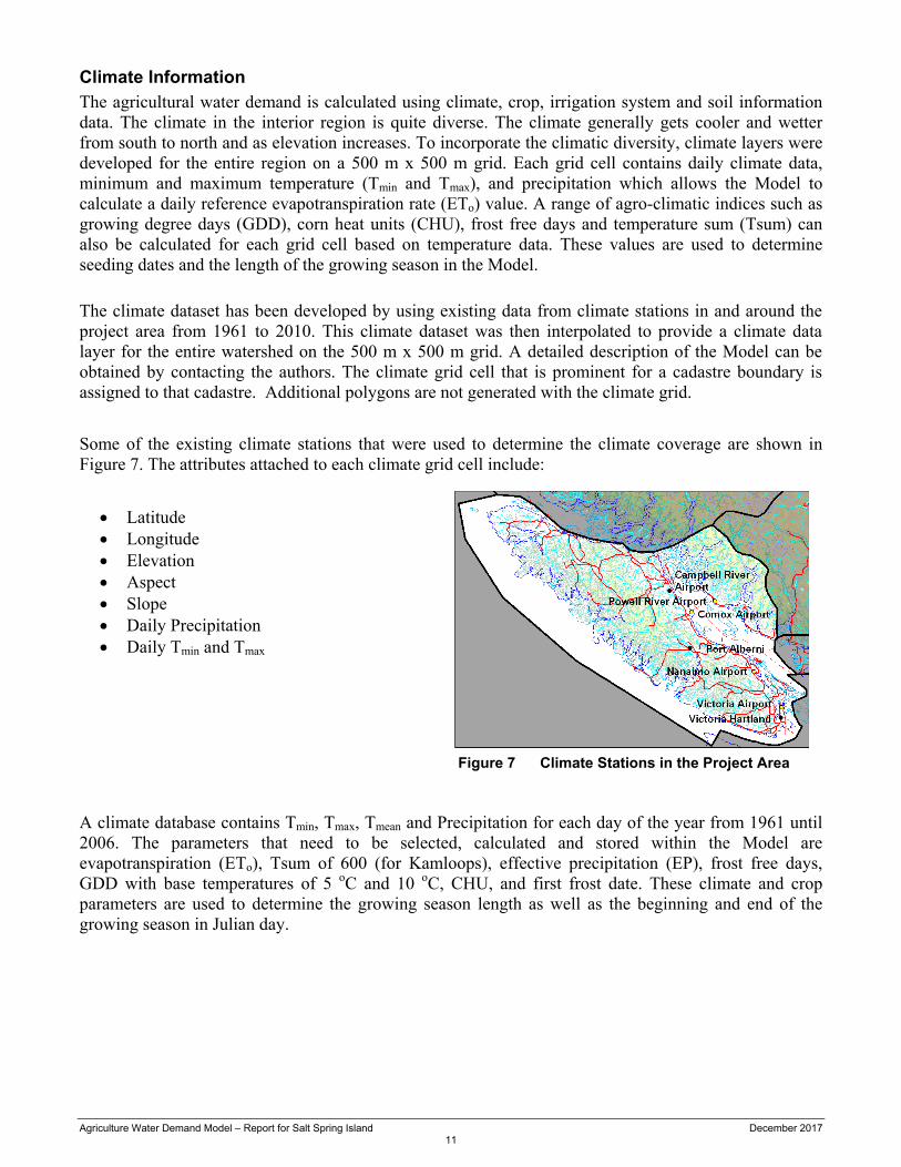
Climate Information The agricultural water demand is calculated using climate, crop, irrigation system and soil information data. The climate in the interior region is quite diverse. The climate generally gets cooler and wetter from south to north and as elevation increases. To incorporate the climatic diversity, climate layers were developed for the entire region on a 500 m x 500 m grid. Each grid cell contains daily climate data, minimum and maximum temperature (Tmin and Tmax), and precipitation which allows the Model to calculate a daily reference evapotranspiration rate (ETo) value. A range of agro-climatic indices such as growing degree days (GDD), corn heat units (CHU), frost free days and temperature sum (Tsum) can also be calculated for each grid cell based on temperature data. These values are used to determine seeding dates and the length of the growing season in the Model.
The climate dataset has been developed by using existing data from climate stations in and around the project area from 1961 to 2010. This climate dataset was then interpolated to provide a climate data layer for the entire watershed on the 500 m x 500 m grid. A detailed description of the Model can be obtained by contacting the authors. The climate grid cell that is prominent for a cadastre boundary is assigned to that cadastre. Additional polygons are not generated with the climate grid.
Some of the existing climate stations that were used to determine the climate coverage are shown in Figure 7. The attributes attached to each climate grid cell include:
Latitude Longitude Elevation Aspect Slope Daily Precipitation Daily Tmin and Tmax
A climate database contains Tmin, Tmax, Tmean and Precipitation for each day of the year from 1961 until 2006. The parameters that need to be selected, calculated and stored within the Model are evapotranspiration (ETo), Tsum of 600 (for Kamloops), effective precipitation (EP), frost free days, GDD with base temperatures of 5 oC and 10 oC, CHU, and first frost date. These climate and crop parameters are used to determine the growing season length as well as the beginning and end of the growing season in Julian day.
Figure 7 Climate Stations in the Project Area
Agriculture Water Demand Model – Report for Salt Spring Island December 2017 12
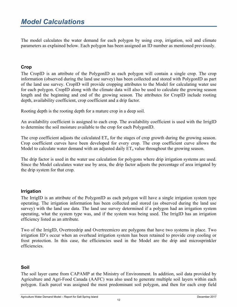
Model Calculations The model calculates the water demand for each polygon by using crop, irrigation, soil and climate parameters as explained below. Each polygon has been assigned an ID number as mentioned previously. Crop The CropID is an attribute of the PolygonID as each polygon will contain a single crop. The crop information (observed during the land use survey) has been collected and stored with PolygonID as part of the land use survey. CropID will provide cropping attributes to the Model for calculating water use for each polygon. CropID along with the climate data will also be used to calculate the growing season length and the beginning and end of the growing season. The attributes for CropID include rooting depth, availability coefficient, crop coefficient and a drip factor. Rooting depth is the rooting depth for a mature crop in a deep soil. An availability coefficient is assigned to each crop. The availability coefficient is used with the IrrigID to determine the soil moisture available to the crop for each PolygonID. The crop coefficient adjusts the calculated ETo for the stages of crop growth during the growing season. Crop coefficient curves have been developed for every crop. The crop coefficient curve allows the Model to calculate water demand with an adjusted daily ETo value throughout the growing season. The drip factor is used in the water use calculation for polygons where drip irrigation systems are used. Since the Model calculates water use by area, the drip factor adjusts the percentage of area irrigated by the drip system for that crop. Irrigation The IrrigID is an attribute of the PolygonID as each polygon will have a single irrigation system type operating. The irrigation information has been collected and stored (as observed during the land use survey) with the land use data. The land use survey determined if a polygon had an irrigation system operating, what the system type was, and if the system was being used. The IrrigID has an irrigation efficiency listed as an attribute. Two of the IrrigID, Overtreedrip and Overtreemicro are polygons that have two systems in place. Two irrigation ID’s occur when an overhead irrigation system has been retained to provide crop cooling or frost protection. In this case, the efficiencies used in the Model are the drip and microsprinkler efficiencies. Soil The soil layer came from CAPAMP at the Ministry of Environment. In addition, soil data provided by Agriculture and Agri-Food Canada (AAFC) was also used to generate multiple soil layers within each polygon. Each parcel was assigned the most predominant soil polygon, and then for each crop field

Agriculture Water Demand Model – Report for Salt Spring Island December 2017 13
within that soil polygon, the most predominant texture within the crop’s rooting depth was determined and assigned to the crop field. Note that textures could repeat at different depths – the combined total of the thicknesses determined the most predominant texture. For example, a layer of 20 cm sand, followed by 40 cm clay and then 30 cm of sand would have sand be designated at the predominant soil texture. The attributes attached to the SoilID is the Available Water Storage Capacity (AWSC) which is calculated using the soil texture and crop rooting depth. The Maximum Soil Water Deficit (MSWD) is calculated to decide the parameters for the algorithm that is used to determine the Irrigation Requirement (IR). The Soil Moisture Deficit at the beginning of the season is calculated using the same terms as the MSWD. Climate The climate data in the Model is used to calculate a daily reference evapotranspiration rate (ETo) for each climate grid cell. The data that is required to calculate this value are:
Elevation, metres (m) Latitude, degrees (o) Minimum Temperature, degree Celsius (oC) Maximum Temperature, degree Celsius (oC) Classification as Coastal or Interior Classification as Arid or Humid Julian Day
Data that is assumed or are constants in this calculation are:
Wind speed 2 m/s Albedo or canopy reflection coefficient, 0.23 Solar constant, Gsc 0.082 MJ-2min-1 Interior and Coastal coefficients, KRs 0.16 for interior locations
0.19 for coastal locations Humid and arid region coefficients, Ko 0 °C for humid/sub-humid climates
2 °C for arid/semi-arid climates Agricultural Water Demand Equation The Model calculates the Agriculture Water Demand (AWD) for each polygon, as a unique crop, irrigation system, soil and climate data is recorded on a polygon basis. The polygons are then summed to determine the AWD for each cadastre. The cadastre water demand values are then summed to determine AWD for the basin, sub-basin, water purveyor or local government. The following steps provide the process used by the Model to calculate Agricultural Water Demand. Detailed information is available on request. 1. Pre-Season Soil Moisture Content
Prior to the start of each crop’s growing season, the soil’s stored moisture content is modelled using the soil and crop evaporation and transpiration characteristics and the daily precipitation values. Precipitation increases the soil moisture content and evaporation (modelled using the
Agriculture Water Demand Model – Report for Salt Spring Island December 2017 14
reference potential evapotranspiration) depletes it. In general, during the pre-season, the soil moisture depth cannot be reduced beyond the maximum evaporation depth; grass crops in wet climates, however, can also remove moisture through crop transpiration. The process used to model the pre-season soil moisture content is:
1. Determine whether the modelling area is considered to be in a wet or dry climate (see Wet/Dry Climate Assessment), and retrieve the early season evaporation factor in the modelling area
2. For each crop type, determine the start of the growing season (see Growing Season Boundaries)
3. For each crop and soil combination, determine the maximum soil water deficit (MSWD) and maximum evaporation factor (maxEvaporation)
4. Start the initial storedMoisture depth on January 1 at the MSWD level 5. For each day between the beginning of the calendar year and the crop’s growing season
start, calculate a new storedMoisture from: a. the potential evapotranspiration (ETo) b. the early season evaporation factor (earlyEvaporationFactor) c. the effective precipitation (EP) = actual precipitation x earlyEvaporationFactor d. daily Climate Moisture Deficit (CMD) = ETo – EP e. storedMoisture = previous day’s storedMoisture – CMD
A negative daily CMD (precipitation in excess of the day’s potential evapotranspiration) adds to the stored moisture level while a positive climate moisture deficit reduces the amount in the stored moisture reservoir. The stored moisture cannot exceed the maximum soil moisture deficit; any precipitation that would take the stored moisture level above the MSWD gets ignored. For all crops and conditions except for grass in wet climates, the stored moisture content cannot drop below the maximum soil water deficit minus the maximum evaporation depth; without any crop transpiration in play, only a certain amount of water can be removed from the soil through evaporative processes alone. Grass in wet climates does grow and remove moisture from the soil prior to the start of the irrigation season however. In those cases, the stored moisture level can drop beyond the maximum evaporation depth, theoretically to 0. Greenhouses and mushroom barns have no stored soil moisture content.
2. In-Season Precipitation
During the growing season, the amount of precipitation considered effective (EP) depends on the overall wetness of the modelling area’s climate (see Wet/Dry Climate Assessment). In dry climates, the first 5 mm of precipitation is ignored, and the EP is calculated as 75% of the remainder: EP = (Precip - 5) x 0.75 In wet climates, the first 5 mm is included in the EP. The EP is 75% of the actual precipitation: EP = Precip x 0.75 Greenhouses and mushroom barns automatically have an EP value of 0.

Agriculture Water Demand Model – Report for Salt Spring Island December 2017 15
3. Crop Cover Coefficient (Kc)
As the crops grow, the amount of water they lose due to transpiration changes. Each crop has a pair of polynomial equations that provide the crop coefficient for any day during the crop’s growing season. It was found that two curves, one for modelling time periods up to the present and one for extending the modelling into the future, provided a better sequence of crop coefficients than using a single curve for all years (currently 1961 to 2100). The application automatically selects the current or future curve as modelling moves across the crop Curve Changeover Year.
For alfalfa crops, there are different sets of equations corresponding to different cuttings
throughout the growing season. 4. Crop Evapotranspiration (ETc)
The evapotranspiration for each crop is calculated as the general ETo multiplied by the crop coefficient (Kc):
ETc = ETo x Kc
5. Climate Moisture Deficit (CMD)
During the growing season, the daily Climate Moisture Deficit (CMD) is calculated as the crop evapotranspiration (ETc) less the Effective Precipitation (EP): CMD = ETc – EP During each crop’s growing season, a stored moisture reservoir methodology is used that is similar to the soil moisture content calculation in the pre-season. On a daily basis, the stored moisture level is used towards satisfying the climate moisture deficit to produce an adjusted Climate Moisture Deficit (CMDa):
CMDa = CMD – storedMoisture If the storedMoisture level exceeds the day’s CMD, then the CMDa is 0 and the stored moisture level is reduced by the CMD amount. If the CMD is greater than the stored moisture, then all of the stored moisture is used (storedMoisture is set to 0) and the adjusted CMD creates an irrigation requirement. The upper limit for the storedMoisture level during the growing season is the maximum soil water deficit (MSWD) setting.
6. Crop Water Requirement (CWR)
The Crop Water Requirement is calculated as the adjusted Climate Moisture Deficit (CMDa) multiplied by the soil water factor (swFactor) and any stress factor (used primarily for grass crops):
CWR = CMDa x swFactor x stressFactor
Agriculture Water Demand Model – Report for Salt Spring Island December 2017 16
7. Irrigation Requirement (IR)
The Irrigation Requirement is the Crop Water Requirement (CWR) after taking into account the irrigation efficiency (Ie) and, for drip systems, the drip factor (Df):
IR = CWR x
Df Ie
For irrigation systems other than drip, the drip factor is 1.
8. The Irrigation Water Demand (IWDperc and IWD)
The portion of the Irrigation Water Demand lost to deep percolation is the Irrigation Requirement (IR) multiplied by the percolation factor (soilPercFactor):
IWDperc = IR x soilPercFactor The final Irrigation Water Demand (IWD) is then the Irrigation Requirement (IR) plus the loss to percolation (IWDperc):
IWD = IR + IWDperc
9. Frost Protection
For some crops (e.g. cranberries), an application of water is often used under certain climatic conditions to provide protection against frost damage. For cranberries, the rule is: when the temperature drops to 0 oC or below between March 16 and May 20 or between October 1 and November 15, a frost event will be calculated. The calculated value is an application of 2.5 mm per hour for 10 hours. In addition, 60% of the water is recirculated and reused, accounting for evaporation and seepage losses.
This amounts to a modelled water demand of 10 mm over the cranberry crop’s area for each day that a frost event occurs between the specified dates.
10. Annual Soil Moisture Deficit
Prior to each crop's growing season, the Model calculates the soil's moisture content by starting it at full (maximum soil water deficit level) on January 1, and adjusting it daily according to precipitation and evaporation. During the growing season, simple evaporation is replaced by the crop's evapotranspiration as it progresses through its growth stages. At the completion of each crop's growing season, an annual soil moisture deficit (SMD) is calculated as the difference between the soil moisture content at that point and the maximum soil water deficit (MSWD):
SMD = MSWD - storedMoisture

Agriculture Water Demand Model – Report for Salt Spring Island December 2017 17
In dry/cold climates, this amount represents water that the farmer would add to the soil in order to prevent it from freezing. Wet climates are assumed to have sufficient precipitation and warm enough temperatures to avoid the risk of freezing without this extra application of water; the SMD demand is therefore recorded only for dry areas. There is no fixed date associated with irrigation to compensate for the annual soil moisture deficit. The farmer may choose to do it any time after the end of the growing season and before the freeze up. In the Model’s summary reports, the water demand associated with the annual soil moisture deficit shows as occurring at time 0 (week 0, month 0, etc.) simply to differentiate it from other demands that do have a date of occurrence during the crop's growing season. Greenhouses and mushroom barns do not have an annual soil moisture deficit.
Agriculture Water Demand Model – Report for Salt Spring Island December 2017 18
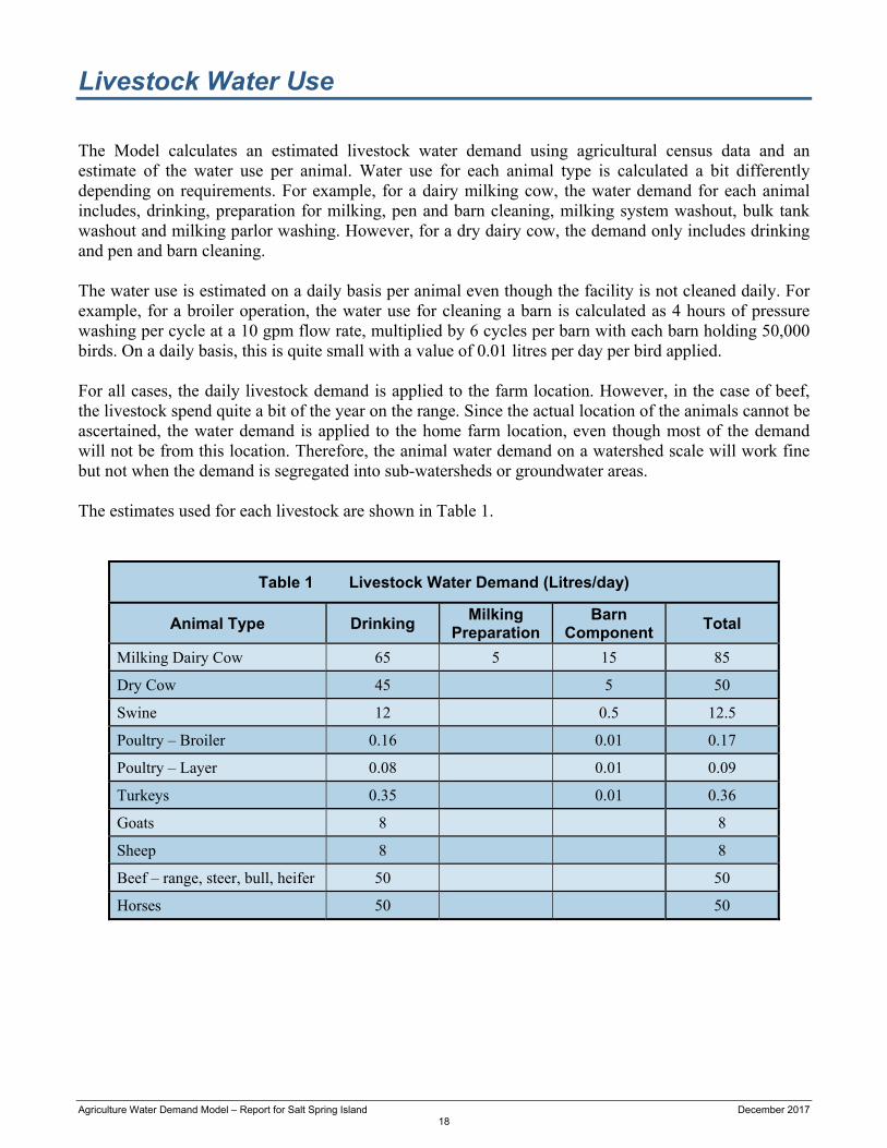
Livestock Water Use The Model calculates an estimated livestock water demand using agricultural census data and an estimate of the water use per animal. Water use for each animal type is calculated a bit differently depending on requirements. For example, for a dairy milking cow, the water demand for each animal includes, drinking, preparation for milking, pen and barn cleaning, milking system washout, bulk tank washout and milking parlor washing. However, for a dry dairy cow, the demand only includes drinking and pen and barn cleaning. The water use is estimated on a daily basis per animal even though the facility is not cleaned daily. For example, for a broiler operation, the water use for cleaning a barn is calculated as 4 hours of pressure washing per cycle at a 10 gpm flow rate, multiplied by 6 cycles per barn with each barn holding 50,000 birds. On a daily basis, this is quite small with a value of 0.01 litres per day per bird applied. For all cases, the daily livestock demand is applied to the farm location. However, in the case of beef, the livestock spend quite a bit of the year on the range. Since the actual location of the animals cannot be ascertained, the water demand is applied to the home farm location, even though most of the demand will not be from this location. Therefore, the animal water demand on a watershed scale will work fine but not when the demand is segregated into sub-watersheds or groundwater areas. The estimates used for each livestock are shown in Table 1.
Table 1 Livestock Water Demand (Litres/day)
Animal Type Drinking Milking
Preparation Barn
Component Total
Milking Dairy Cow 65 5 15 85
Dry Cow 45 5 50
Swine 12 0.5 12.5
Poultry – Broiler 0.16 0.01 0.17
Poultry – Layer 0.08 0.01 0.09
Turkeys 0.35 0.01 0.36
Goats 8 8
Sheep 8 8
Beef – range, steer, bull, heifer 50 50
Horses 50 50

Agriculture Water Demand Model – Report for Salt Spring Island December 2017 19
Definition and Calculation of Individual Terms Used in the Irrigation Water Demand Equation Growing Season Boundaries There are three sets of considerations used in calculating the start and end of the irrigation season for each crop:
temperature-based growing season derivations, generally using Temperature Sum (Tsum) or Growing Degree Day (GDD) accumulations
the growing season overrides table the irrigation season overrides table
These form an order of precedence with later considerations potentially overriding the dates established for the previous rules. For example, the temperature-based rules might yield a growing season start date of day 90 for a given crop in a mild year. To avoid unrealistic irrigation starts, the season overrides table might enforce a minimum start day of 100 for that crop; at that point, the season start would be set to day 100. At the same time, a Water Purveyor might not turn on the water supply until day 105; specifying that as the minimum start day in the irrigation season overrides table would prevent any irrigation water demands until day 105. This section describes the rules used to establish growing season boundaries based on the internal calculations of the Model. The GDD and Tsum Day calculations are described in separate sections. The standard end of season specified for several crops is the earlier of the end date of Growing Degree Day with base temperature of 5 oC (GDD5) or the first frost. 1. Corn (silage corn)
uses the corn_start date for the season start season end: earlier of the killing frost or the day that the CHU2700 (2700 Corn Heat Units)
threshold is reached
2. Sweetcorn, Potato, Tomato, Pepper, Strawberry, Vegetable, Pea corn_start date for the season start corn start plus 110 days for the season end
3. Cereal GDD5 start for the season start GDD5 start plus 130 days for the season end
4. AppleHD, AppleMD, AppleLD, Asparagus, Berry, Blueberry, Ginseng, Nuts, Raspberry, Sourcherry, Treefruit, Vineberry season start: (0.8447 x tsum600_day) + 18.877 standard end of season
5. Pumpkin corn_start date standard end of season

Agriculture Water Demand Model – Report for Salt Spring Island December 2017 20
6. Apricot season start: (0.9153 x tsum400_day) + 5.5809 standard end of season
7. CherryHD, CherryMD, CherryLD
season start: (0.7992 x tsum450_day) + 24.878 standard end of season
8. Grape, Kiwi season start: (0.7992 x tsum450_day) + 24.878 standard end of season
9. Peach, Nectarine season start: (0.8438 x tsum450_day) + 19.68 standard end of season
10. Plum season start: (0.7982 x tsum500_day) + 25.417 standard end of season
11. Pear season start: (0.8249 x tsum600_day) + 17.14 standard end of season
12. Golf, TurfFarm season start: later of the GDD5 start and the tsum300_day standard end of season
13. Domestic, Yard, TurfPark season start: later of the GDD5 start and the tsum400_day standard end of season
14. Greenhouse (interior greenhouses) fixed season of April 1 – October 30
15. GH Tomato, GH Pepper, GH Cucumber fixed season of January 15 – November 30
16. GH Flower fixed season of March 1 – October 30
17. GH Nursery fixed season of April 1 – October 30
18. Mushroom all year: January 1 – December 31
Agriculture Water Demand Model – Report for Salt Spring Island December 2017 21
19. Shrubs/Trees, Fstock, NurseryPOT season start: tsum500_day end: Julian day 275
20. Floriculture season start: tsum500_day end: Julian day 225
21. Cranberry season start: tsum500_day end: Julian day 275
22. Grass, Forage, Alfalfa, Pasture season start: later of the GDD5 and the tsum600_day standard end of season
23. Nursery season start: tsum400_day standard end of season
Evapotranspiration (ETo) The ETo calculation follows the FAO Penman-Montieth equation. Two modifications were made to the equation:
Step 6 – Inverse Relative Distance Earth-Sun (dr) Instead of a fixed 365 days as a divisor, the actual number of days for each year (365 or 366) was used.
Step 19 – Evapotranspiration (ETo)
For consistency, a temperature conversion factor of 273.16 was used instead of the rounded 273 listed.
Availability Coefficient (AC) The availability coefficient is a factor representing the percentage of the soil’s total water storage that the crop can readily extract. The factor is taken directly from the crop factors table (crop_factors) based on the cropId value. Rooting Depth (RD) The rooting depth represents the crop’s maximum rooting depth and thus the depth of soil over which the plant interacts with the soil in terms of moisture extraction. The value is read directly from the crop factors table.
Agriculture Water Demand Model – Report for Salt Spring Island December 2017 22
Stress Factor (stressFactor) Some crops, such as grasses, are often irrigated to a less degree than their full theoretical requirement for optimal growth. The stress factor (crop_groups_and_factors) reduces the calculated demand for these crops. Available Water Storage Capacity (AWSC) The available water storage capacity is a factor representing the amount of water that a particular soil texture can hold without the water dropping through and being lost to deep percolation. The factor is taken directly from the soil factors table (soil_factors). Maximum Soil Water Deficit (MSWD) The maximum soil water deficit is the product of the crop’s availability coefficient, rooting depth, and the available water storage capacity of the soil:
ACAWSCRDMSWD Deep Percolation Factor (Soilpercfactor) The soil percolation factor is used to calculate the amount of water lost to deep percolation under different management practices. For greenhouse crops, the greenhouse leaching factor is used as the basic soil percolation factor. This is then multiplied by a greenhouse recirculation factor, if present, to reflect the percentage of water re-captured and re-used in greenhouse operations. soilPercFactor = soilPercFactor x (1 – recirculationFactor) For Nursery Pot (Nursery POT) and Forestry Stock (Fstock) crops, the soil percolation factor is fixed at 35%. For other crops, the factor depends on the soil texture, the MSWD, the irrigation system, and the Irrigation Management Practices code. The percolation factors table (soil_percolation_factors) is read to find the first row with the correct management practices, soil texture and irrigation system, and a MSWD value that matches or exceeds the value calculated for the current land use polygon. If the calculated MSWD value is greater than the index value for all rows in the percolation factors table, then the highest MSWD factor is used. If there is no match based on the passed parameters, then a default value of 0.25 is applied. For example, a calculated MSWD value of 82.5 mm, a soil texture of sandy loam (SL) and an irrigation system of solid set overtree (Ssovertree) would retrieve the percolation factor associated with the MSWD index value of 75 mm in the current table (presently, there are rows for MSWD 50 mm and 75 mm for SL and Ssovertree).

Agriculture Water Demand Model – Report for Salt Spring Island December 2017 23
Maximum Evaporation Factor (maxEvaporation) Just as different soil textures can hold different amounts of water, they also have different depths that can be affected by evaporation. The factor is taken directly from the soil factors table.
Irrigation Efficiency (Ie) Each irrigation system type has an associated efficiency factor (inefficient systems require the application of more water in order to satisfy the same crop water demand). The factor is read directly from the irrigation factors table (irrigation_factors). Soil Water Factor (swFactor) For the greenhouse “crop”, the soil water factor is set to 1. For other crops, it is interpolated from a table (soil_water_factors) based on the MSWD. For Nurseries, the highest soil water factor (lowest MSWD index) in the table is used; otherwise, the two rows whose MSWD values bound the calculated MSWD are located and a soil water factor interpolated according to where the passed MSDW value lies between those bounds. For example, using the current table with rows giving soil water factors of 0.95 and 0.9 for MSWD index values of 75 mm and 100 mm respectively, a calculated MSWD value of 82.5 mm would return a soil water factor of:
935.0
95.09.075100
755.8295.0
If the calculated MSWD value is higher or lower than the index values for all of the rows in the table, then the factor associated with the highest or lowest MSWD index is used. Early Season Evaporation Factor (earlyEvaporationFactor) The effective precipitation (precipitation that adds to the stored soil moisture content) can be different in the cooler pre-season than in the growing season. The early season evaporation factor is used to determine what percentage of the precipitation is considered effective prior to the growing season. Crop Coefficient (Kc) The crop coefficient is calculated from a set of fourth degree polynomial equations representing the crop’s ground coverage throughout its growing season. The coefficients for each term are read from the crop factors table based on the crop type, with the variable equalling the number of days since the start of the crop’s growing season. For example, the crop coefficient for Grape on day 35 of the growing season would be calculated as: Kc = [0.0000000031 x (35)4] + [-0.0000013775 x (35)3] + (0.0001634536 x (35)2] + (-0.0011179845 x 35) + 0.2399004137 = 0.346593241
Agriculture Water Demand Model – Report for Salt Spring Island December 2017 24
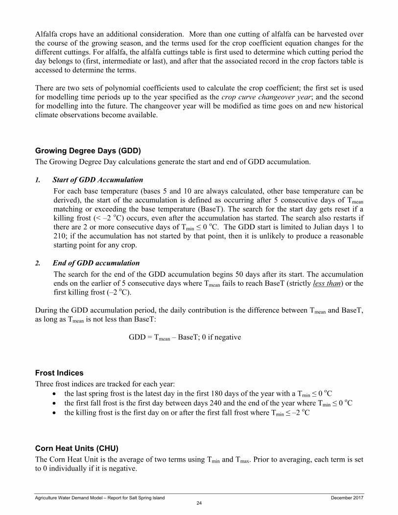
Alfalfa crops have an additional consideration. More than one cutting of alfalfa can be harvested over the course of the growing season, and the terms used for the crop coefficient equation changes for the different cuttings. For alfalfa, the alfalfa cuttings table is first used to determine which cutting period the day belongs to (first, intermediate or last), and after that the associated record in the crop factors table is accessed to determine the terms. There are two sets of polynomial coefficients used to calculate the crop coefficient; the first set is used for modelling time periods up to the year specified as the crop curve changeover year; and the second for modelling into the future. The changeover year will be modified as time goes on and new historical climate observations become available. Growing Degree Days (GDD) The Growing Degree Day calculations generate the start and end of GDD accumulation. 1. Start of GDD Accumulation
For each base temperature (bases 5 and 10 are always calculated, other base temperature can be derived), the start of the accumulation is defined as occurring after 5 consecutive days of Tmean matching or exceeding the base temperature (BaseT). The search for the start day gets reset if a killing frost (< –2 oC) occurs, even after the accumulation has started. The search also restarts if there are 2 or more consecutive days of Tmin ≤ 0 oC. The GDD start is limited to Julian days 1 to 210; if the accumulation has not started by that point, then it is unlikely to produce a reasonable starting point for any crop.
2. End of GDD accumulation
The search for the end of the GDD accumulation begins 50 days after its start. The accumulation ends on the earlier of 5 consecutive days where Tmean fails to reach BaseT (strictly less than) or the first killing frost (–2 oC).
During the GDD accumulation period, the daily contribution is the difference between Tmean and BaseT, as long as Tmean is not less than BaseT: GDD = Tmean – BaseT; 0 if negative Frost Indices Three frost indices are tracked for each year:
the last spring frost is the latest day in the first 180 days of the year with a Tmin ≤ 0 oC the first fall frost is the first day between days 240 and the end of the year where Tmin ≤ 0 oC the killing frost is the first day on or after the first fall frost where Tmin ≤ –2 oC
Corn Heat Units (CHU) The Corn Heat Unit is the average of two terms using Tmin and Tmax. Prior to averaging, each term is set to 0 individually if it is negative.
Agriculture Water Demand Model – Report for Salt Spring Island December 2017 25
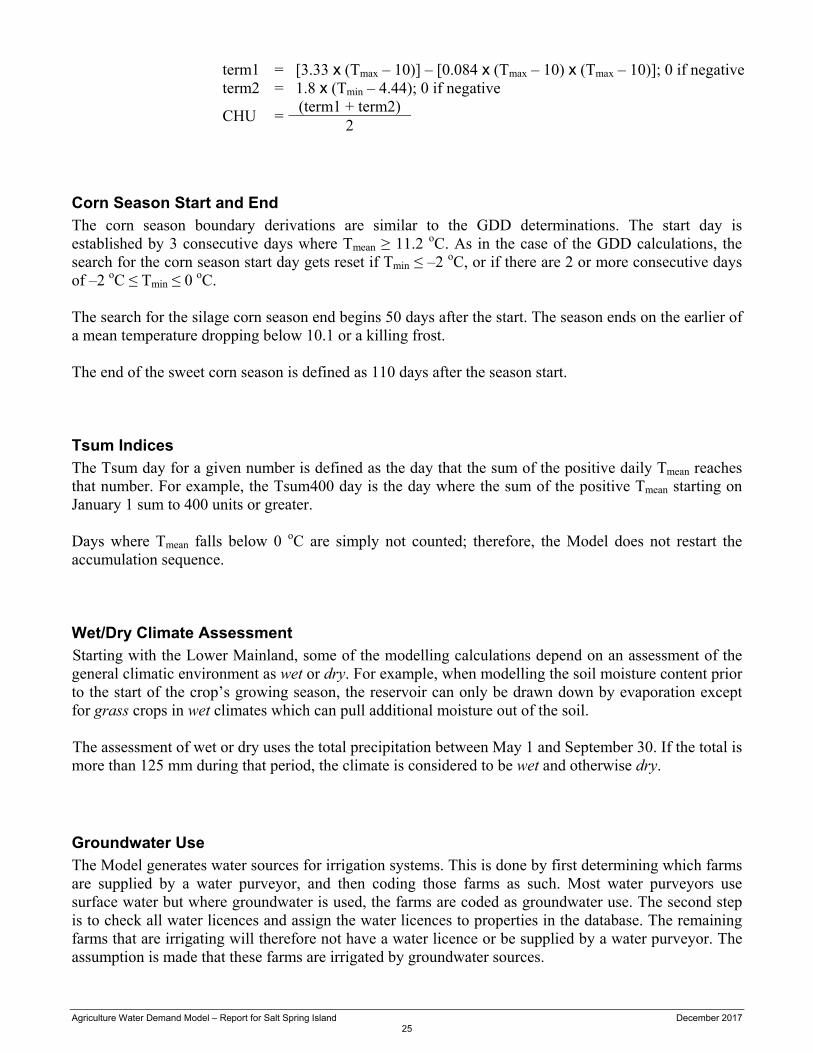
term1 = [3.33 x (Tmax – 10)] – [0.084 x (Tmax – 10) x (Tmax – 10)]; 0 if negative term2 = 1.8 x (Tmin – 4.44); 0 if negative
CHU = (term1 + term2)
2
Corn Season Start and End The corn season boundary derivations are similar to the GDD determinations. The start day is established by 3 consecutive days where Tmean ≥ 11.2 oC. As in the case of the GDD calculations, the search for the corn season start day gets reset if Tmin ≤ –2 oC, or if there are 2 or more consecutive days of –2 oC ≤ Tmin ≤ 0 oC. The search for the silage corn season end begins 50 days after the start. The season ends on the earlier of a mean temperature dropping below 10.1 or a killing frost. The end of the sweet corn season is defined as 110 days after the season start. Tsum Indices The Tsum day for a given number is defined as the day that the sum of the positive daily Tmean reaches that number. For example, the Tsum400 day is the day where the sum of the positive Tmean starting on January 1 sum to 400 units or greater. Days where Tmean falls below 0 oC are simply not counted; therefore, the Model does not restart the accumulation sequence. Wet/Dry Climate Assessment Starting with the Lower Mainland, some of the modelling calculations depend on an assessment of the general climatic environment as wet or dry. For example, when modelling the soil moisture content prior to the start of the crop’s growing season, the reservoir can only be drawn down by evaporation except for grass crops in wet climates which can pull additional moisture out of the soil. The assessment of wet or dry uses the total precipitation between May 1 and September 30. If the total is more than 125 mm during that period, the climate is considered to be wet and otherwise dry.
Groundwater Use The Model generates water sources for irrigation systems. This is done by first determining which farms are supplied by a water purveyor, and then coding those farms as such. Most water purveyors use surface water but where groundwater is used, the farms are coded as groundwater use. The second step is to check all water licences and assign the water licences to properties in the database. The remaining farms that are irrigating will therefore not have a water licence or be supplied by a water purveyor. The assumption is made that these farms are irrigated by groundwater sources.

Agriculture Water Demand Model – Report for Salt Spring Island December 2017 26
Land Use Results A summary of the land area and the inventoried project area are shown in Table 2. The inventoried area includes parcels that are in and partially in the Agricultural Land Reserve (ALR).
Table 2 Overview of the Land and Inventoried Area
Area Type Area (ha)
Salt Spring Island (SSI)
Total Area 486,743
Area of Water Feature 12,153
Area of Land (excluding water features) 18,272
ALR Area 14,074
Inventoried Area
Total Inventoried Area 6,213
Out of the total inventoried area, there are:
1,078 ha of cultivated crops within which only 99 ha are currently being irrigated and 135 are inactively farmed.
over 4,000 ha of land that are natural and semi-natural areas (not being farmed) Over 400 ha that are anthropogenically modified in buildings, roads and landscaped (not being
farmed) The primary agricultural use of the ARL area is shown in Table 3. Refer to the Agricultural Land Use Inventory (ALUI) report for details.
Table 3 Summary of Primary Agricultural Activities within the ALR where Primary Land Use is agriculture in the Project Area
Primary Agriculture Activity Total Land Cover (ha)
Vegetables 34
Forage 29
Grape 13
Tree Fruits 8
Nursery and Tree Plantations 7
Berries 3
Others 5
Total 99
Agriculture Water Demand Model – Report for Salt Spring Island December 2017 27
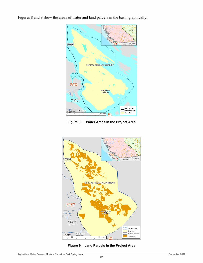
Figures 8 and 9 show the areas of water and land parcels in the basin graphically.
Figure 8 Water Areas in the Project Area
Figure 9 Land Parcels in the Project Area

Agriculture Water Demand Model – Report for Salt Spring Island December 2017 28
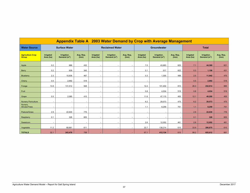
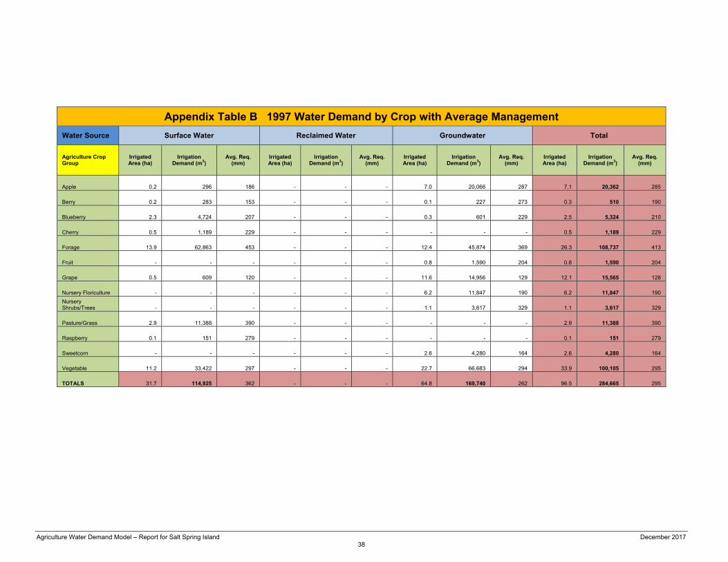
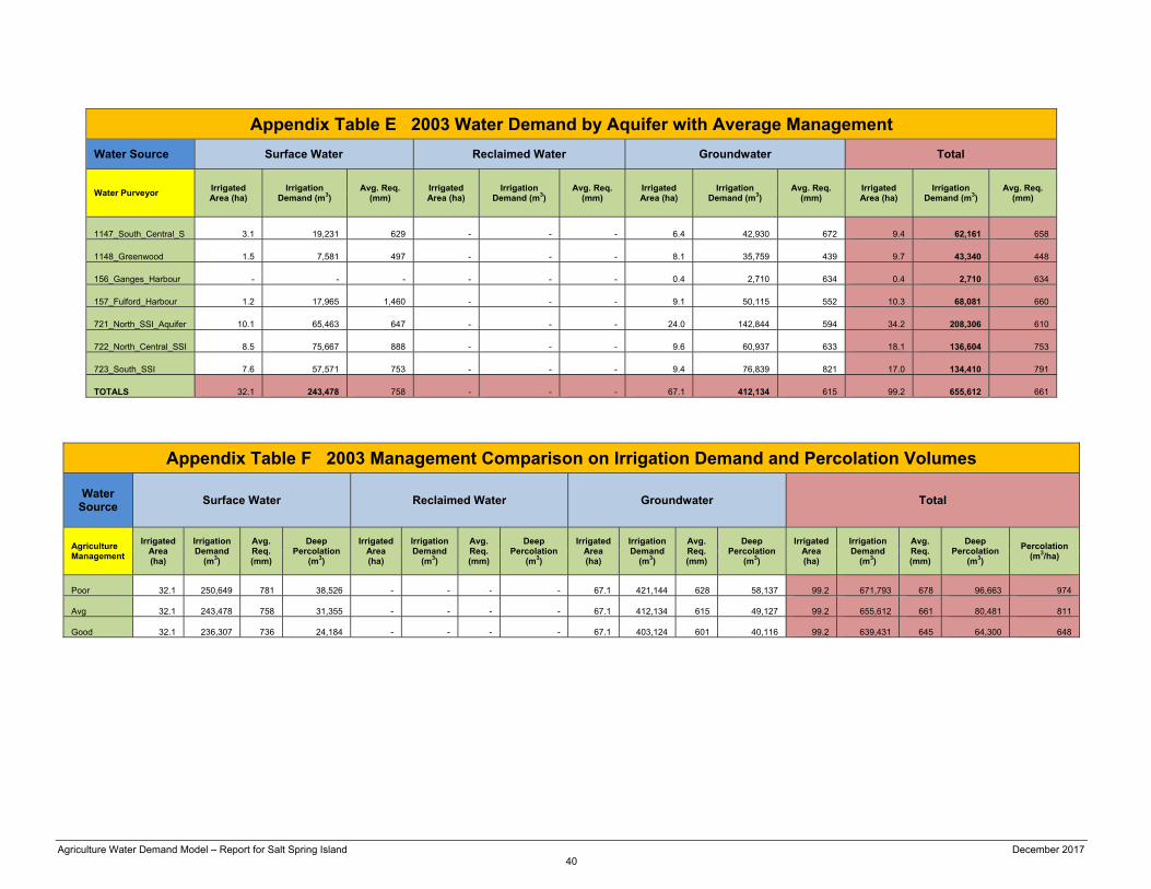
Agricultural Water Demand Results The Model has a reporting feature that can save and generate reports for many different scenarios that have been pre-developed. This report will provide a summary of the reported data in the Appendices. Climate data from 1997 and 2003 were chosen as they represent a relatively wet year and dry year respectively. Most reports are based on the 2003 data since the maximum current demand can then be presented. Scenarios using climate change information in the 2050’s is also presented. Annual Crop Water Demand – Tables A and B The Model can use three different irrigation management factors, good, average and poor. Unless otherwise noted, average management were used in the tables. Appendix Table A provides the annual irrigation water demand for current crop and irrigation systems used for the year 2003 using average irrigation management, and Table B provides the same data for 1997. Where a crop was not established, the acreage was assigned a forage crop so that the Model could determine a water demand. The total irrigated acreage in SSI is 99 hectares (ha), including 34 ha of vegetables and 29 ha of forage crops (alfalfa, forage corn, grass, legume and pasture). In SSI, 32 ha is supplied by licensed surface water sources, and 67 ha is irrigated with groundwater. The total annual irrigation demand was 655,612 m3 in 2003, and dropped to 284,665 m3 in 1997. During a wet year like 1997, the demand was only 43% of a hot dry year like 2003. In addition, the Model also calculates demand based on relatively good practices. As such, actual use may actually be higher or lower than what is calculated by the Model. Annual Water Demand by Irrigation System – Table C The crop irrigation demand can also be reported by irrigation system type as shown in Table C. The more efficient irrigation system for vegetable is drip (including overtreedrip) which irrigates 24 ha in the project area, and for forage is low-pressure pivots which are not being used in this area. There is also a large portion of the vegetables irrigated by sprinkler systems (including travelling guns and solid set guns). Sprinkler, solid set guns, and travelling guns irrigate 70 ha of the agricultural crops. Annual Water Demand by Soil Texture – Table D Table D provides annual water demand by soil texture. Where soil texture data is missing, the soil texture has been defaulted to sandy loam. The defaults are shown in Table D. Annual Water Demand by Aquifer – Table E The model calculates water demand on a property by property basis and can summarize the data for each aquifer in the project area. Table E provides an estimated water demand for each aquifer. Irrigation Management Factors – Table F The Model can estimate water demand based on poor, average and good irrigation management factors. This is accomplished by developing an irrigation management factor for each crop, soil and irrigation
Agriculture Water Demand Model – Report for Salt Spring Island December 2017 29
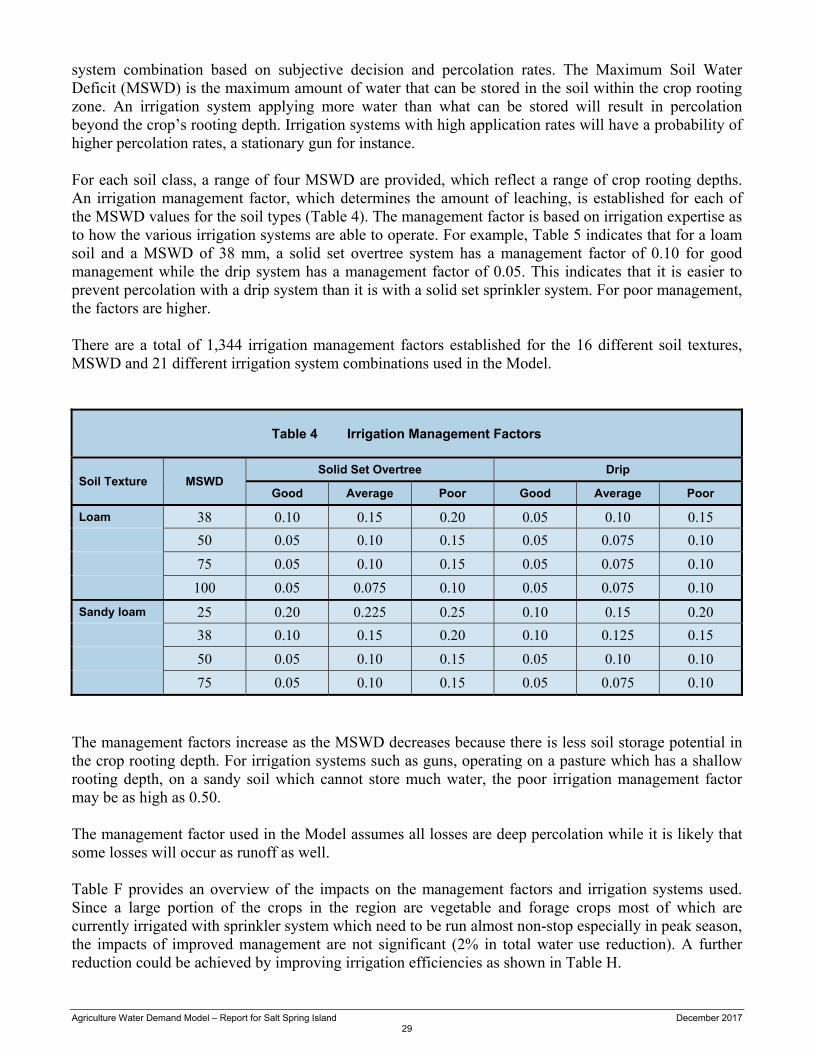
system combination based on subjective decision and percolation rates. The Maximum Soil Water Deficit (MSWD) is the maximum amount of water that can be stored in the soil within the crop rooting zone. An irrigation system applying more water than what can be stored will result in percolation beyond the crop’s rooting depth. Irrigation systems with high application rates will have a probability of higher percolation rates, a stationary gun for instance. For each soil class, a range of four MSWD are provided, which reflect a range of crop rooting depths. An irrigation management factor, which determines the amount of leaching, is established for each of the MSWD values for the soil types (Table 4). The management factor is based on irrigation expertise as to how the various irrigation systems are able to operate. For example, Table 5 indicates that for a loam soil and a MSWD of 38 mm, a solid set overtree system has a management factor of 0.10 for good management while the drip system has a management factor of 0.05. This indicates that it is easier to prevent percolation with a drip system than it is with a solid set sprinkler system. For poor management, the factors are higher. There are a total of 1,344 irrigation management factors established for the 16 different soil textures, MSWD and 21 different irrigation system combinations used in the Model.
Table 4 Irrigation Management Factors
Soil Texture MSWD Solid Set Overtree Drip
Good Average Poor Good Average Poor
Loam 38 0.10 0.15 0.20 0.05 0.10 0.15
50 0.05 0.10 0.15 0.05 0.075 0.10
75 0.05 0.10 0.15 0.05 0.075 0.10
100 0.05 0.075 0.10 0.05 0.075 0.10
Sandy loam 25 0.20 0.225 0.25 0.10 0.15 0.20
38 0.10 0.15 0.20 0.10 0.125 0.15
50 0.05 0.10 0.15 0.05 0.10 0.10
75 0.05 0.10 0.15 0.05 0.075 0.10
The management factors increase as the MSWD decreases because there is less soil storage potential in the crop rooting depth. For irrigation systems such as guns, operating on a pasture which has a shallow rooting depth, on a sandy soil which cannot store much water, the poor irrigation management factor may be as high as 0.50. The management factor used in the Model assumes all losses are deep percolation while it is likely that some losses will occur as runoff as well. Table F provides an overview of the impacts on the management factors and irrigation systems used. Since a large portion of the crops in the region are vegetable and forage crops most of which are currently irrigated with sprinkler system which need to be run almost non-stop especially in peak season, the impacts of improved management are not significant (2% in total water use reduction). A further reduction could be achieved by improving irrigation efficiencies as shown in Table H.
Agriculture Water Demand Model – Report for Salt Spring Island December 2017 30
This table also provides percolation rates based on good, average and poor management using 2003 climate data. In summary, good management is 64,300 m3, average is 80,481 m3and poor management is 96,663 m3. Percolation rates for poor management are 33% higher than for good management. Deep Percolation – Table G The percolation rates vary by crop, irrigation system type, soil and the management factor used. Table G shows the deep percolation amounts by irrigation system type for average management. The last column provides a good indication of the average percolation per hectare for the various irrigation system types. For example, drip irrigation systems have only about 60% of the percolation rates of gun systems.
Improved Irrigation Efficiency and Good Management – Table H There is an opportunity to reduce water use by converting irrigation systems to a higher efficiency for some crops. For example, drip systems could be used for all fruit crops, vegetable crops and some of the other horticultural crops, but not forage crops. In addition, using better management such as irrigation scheduling techniques will also reduce water use, especially for forage where drip conversion is not possible. Table H provides a scenario of water demand if all sprinkler systems are converted to drip systems for horticultural crops in the project area, as well as converting irrigation systems to low-pressure pivot systems for forage fields over 10 ha, using good irrigation management. In this case, the water demand for 2003 would reduce from 655,612 m3 to 516,257 m3 (27% reduction). Livestock Water Use – Table I The Model provides an estimate of water use for livestock. The estimate is based on the number of animals in the project area as determined by the latest census, the drinking water required for each animal per day and the barn or milking parlour wash water. Values used are shown in Table 1. For the project area, the amount of livestock water is estimated at 48,781 m3. Climate Change Water Demand for 2050 – Table J The Model also has access to climate change information until the year 2100. While data can be run for each year, three driest years in the 2050’s were selected to give a representation of climate change. Figure 10 shows the climate data results which indicate that 2053, 2056, and 2059 generate the highest annual ETo and lowest annual precipitation. These three years were used in this report. Table J provides the results of climate change on irrigation demand for the three years selected using current crops and irrigation systems. Current crops and irrigation systems are used to show the increase due to climate change only, with no other changes taking place. Figure 11 shows all of the climate change scenario runs for the Okanagan using 12 climate models from 1960 to 2100. This work was compiled by Denise Neilsen at the Agriculture and Agri-Food Canada – Summerland Research and Development Centre. There is a lot of scatter in this figure, but it is obvious that there is a trend of increasing water demand.

Agriculture Water Demand Model – Report for Salt Spring Island December 2017 31
The three climate change models used in this report are access1 rcp85, canESM2 rcp85 and cnrm-cm5 rcp85. Running only three climate change models on three selected future years in the project area is not sufficient to provide a trend like in Figure 11. What the results do show is that in an extreme climate scenario, it is possible to have an annual water demand that is 20% higher than what was experienced in 2003 based on canESM2 rcp85 climate model in 2053. More runs of the climate change models will be required to better estimate a climate change trend for the region.
Figure 10 Annual ET and Effective Precipation in 2050's

Agriculture Water Demand Model – Report for Salt Spring Island December 2017 32
Agricultural Buildout Crop Water Demand Using 2003 Climate Data – Table K An agricultural irrigated buildout scenario was developed that looked at potential agricultural lands that could be irrigated in the future. The rules used to establish where potential additional agricultural lands were located are as follows:
within 1,000 m of water supply (lake) within 1,000 m of water supply (water course) within 1,000 m of water supply (wetland) within 1,000 m of high productivity aquifer within 1,000 m of water purveyor with Ag Capability class 1-4 only where available must be within the ALR below 750 m average elevation must be private ownership
Physical structure (e.g., farmstead, houses) are not considered to be available for the buildout scenario. For the areas that are determined to be eligible for future buildout, a crop and irrigation system need to be applied. Where a crop already existed in the land use inventory, that crop would remain and an irrigation system assigned. If no crop existed, then a crop and an irrigation system are assigned as per the criteria below:
70% Vegetable – 70% drip, 30% sprinkler 30% Forage – 50% pivot, 30% sprinkler, 20% travelling gun
Figure 11 Future Irrigation Demand for All Outdoor Uses in the Okanagan in Response to Observed Climate Data (Actuals) and Future Climate Data Projected from a Range of Global
Climate Models
Agriculture Water Demand Model – Report for Salt Spring Island December 2017 33
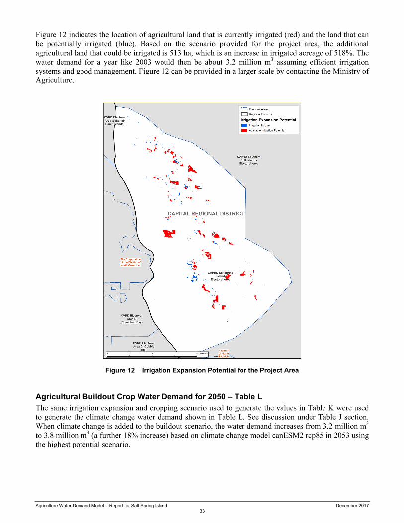
Figure 12 indicates the location of agricultural land that is currently irrigated (red) and the land that can be potentially irrigated (blue). Based on the scenario provided for the project area, the additional agricultural land that could be irrigated is 513 ha, which is an increase in irrigated acreage of 518%. The water demand for a year like 2003 would then be about 3.2 million m3 assuming efficient irrigation systems and good management. Figure 12 can be provided in a larger scale by contacting the Ministry of Agriculture.
Figure 12 Irrigation Expansion Potential for the Project Area Agricultural Buildout Crop Water Demand for 2050 – Table L The same irrigation expansion and cropping scenario used to generate the values in Table K were used to generate the climate change water demand shown in Table L. See discussion under Table J section. When climate change is added to the buildout scenario, the water demand increases from 3.2 million m3 to 3.8 million m3 (a further 18% increase) based on climate change model canESM2 rcp85 in 2053 using the highest potential scenario.
Agriculture Water Demand Model – Report for Salt Spring Island December 2017 34
Irrigation Systems Used for the Buildout Scenario for 2003 – Table M Table M provides an account of the irrigation systems used by area for the buildout scenario in the previous two examples. Note that pivot irrigation (especially low-pressure type) is expected to be used for forage field over 10 ha in size to be economically feasible. Water Demand for the Buildout Area by Aquifer 2003 Climate Data – Table N Table N provides the water demand by water purveyors for the buildout scenario used in this report. Comparing these values with the result in Table E will provide information on the possible increased water demand from groundwater source for the projected irrigated areas. The Model does not determine that there is sufficient groundwater available, only that this would be the potential demand. Note that all the aquifers in this project area have low productivity of groundwater based on the information from BC Ministry of Environment.
Agriculture Water Demand Model – Report for Salt Spring Island December 2017 35
Literature Cannon, A.J., and Whitfield, P.H. (2002), Synoptic map classification using recursive partitioning and principle component analysis. Monthly Weather Rev. 130:1187-1206. Cannon, A.J. (2008), Probabilistic multi-site precipitation downscaling by an expanded Bernoulli-gamma density network. Journal of Hydrometeorology. http://dx.doi.org/10.1175%2F2008JHM960.1 Intergovernmental Panel on Climate Change (IPCC) (2008), Fourth Assessment Report –AR4. http://www.ipcc.ch/ipccreports/ar4-syr.htm Merritt, W, Alila, Y., Barton, M., Taylor, B., Neilsen, D., and Cohen, S. 2006. Hydrologic response to scenarios of climate change in the Okanagan Basin, British Columbia. J. Hydrology. 326: 79-108. Neilsen, D., Smith, S., Frank, G., Koch, W., Alila, Y., Merritt, W., Taylor, B., Barton, M, Hall, J. and Cohen, S. 2006. Potential impacts of climate change on water availability for crops in the Okanagan Basin, British Columbia. Can. J. Soil Sci. 86: 909-924. Neilsen, D., Duke, G., Taylor, W., Byrne, J.M., and Van der Gulik T.W. (2010). Development and Verification of Daily Gridded Climate Surfaces in the Okanagan Basin of British Columbia. Canadian Water Resources Journal 35(2), pp. 131-154. http://www4.agr.gc.ca/abstract-resume/abstract-resume.htm?lang=eng&id=21183000000448 Allen, R. G., Pereira, L. S., Raes, D. and Smith, M. 1998. Crop evapotranspiration Guidelines for computing crop water requirements. FAO Irrigation and Drainage Paper 56. United Nations Food and Agriculture Organization. Rome. 100pp
Agriculture Water Demand Model – Report for Salt Spring Island December 2017 36
Appendix Tables Appendix Table A 2003 Water Demand by Crop with Average Management Appendix Table B 1997 Water Demand by Crop with Average Management Appendix Table C 2003 Water Demand by Irrigation System with Average Management Appendix Table D 2003 Water Demand by Soil Texture with Average Management Appendix Table E 2003 Water Demand by Aquifer with Average Management Appendix Table F 2003 Management Comparison on Irrigation Demand and Percolation Volumes Appendix Table G 2003 Percolation Volumes by Irrigation System with Average Management Appendix Table H 2003 Crop Water Demand for Improved Irrigation System Efficiency and Good Management Appendix Table I 2003 Water Demand by Animal Type with Average Management Appendix Table J Climate Change Water Demand Circa 2050 for a High Demand Year with Good Management using Current Crops and Irrigation Systems Appendix Table K Buildout Crop Water Demand for 2003 Climate Data and Good Management Appendix Table L Buildout Crop Water Demand for Climate Change Circa 2050 and Good Management Appendix Table M Buildout Irrigation System Demand for 2003 Climate Data and Good Management Appendix Table N Buildout Water Demand by Aquifer for 2003 Climate Data and Good Management
Agriculture Water Demand Model – Report for Salt Spring Island December 2017 37
Appendix Table A 2003 Water Demand by Crop with Average Management
Water Source Surface Water Reclaimed Water Groundwater Total
Agriculture Crop Group
Irrigated Area (ha)
Irrigation Demand (m3)
Avg. Req. (mm)
Irrigated Area (ha)
Irrigation Demand (m3)
Avg. Req. (mm)
Irrigated Area (ha)
Irrigation Demand (m3)
Avg. Req. (mm)
Irrigated Area (ha)
Irrigation Demand (m3)
Avg. Req. (mm)
Apple
0.2
686
432
-
-
-
7.0
43,683
625
7.1 44,369
621
Berry
0.2
639
345
-
-
-
0.1
517
622
0.3 1,156
431
Blueberry
2.3
10,636
467
-
-
-
0.3
1,305
498
2.5 11,942
470
Cherry
0.5
2,692
519
-
-
-
-
-
-
0.5 2,692
519
Forage
13.9
131,512
948
-
-
-
12.4
101,402
815
26.3 232,914
885
Fruit
-
-
-
-
-
-
0.8
4,034
519
0.8 4,034
519
Grape
0.5
2,085
410
-
-
-
11.6
47,115
405
12.1 49,200
405
Nursery Floriculture
-
-
-
-
-
-
6.2
29,573
475
6.2 29,573
475
Nursery Shrubs/Trees
-
-
-
-
-
-
1.1
8,259
751
1.1 8,259
751
Pasture/Grass
2.9
22,630
776
-
-
-
-
-
-
2.9 22,630
776
Raspberry
0.1
328
605
-
-
-
-
-
-
0.1 328
605
Sweetcorn
-
-
-
-
-
-
2.6
12,052
461
2.6 12,052
461
Vegetable
11.2
68,661
611
-
-
-
22.7
138,214
610
33.9 206,875
610
TOTALS
32.1 243,478
758
-
-
-
67.1 412,134
615
99.2 655,612
661
Agriculture Water Demand Model – Report for Salt Spring Island December 2017 38
Appendix Table B 1997 Water Demand by Crop with Average Management
Water Source Surface Water Reclaimed Water Groundwater Total
Agriculture Crop Group
Irrigated Area (ha)
Irrigation Demand (m3)
Avg. Req. (mm)
Irrigated Area (ha)
Irrigation Demand (m3)
Avg. Req. (mm)
Irrigated Area (ha)
Irrigation Demand (m3)
Avg. Req. (mm)
Irrigated Area (ha)
Irrigation Demand (m3)
Avg. Req. (mm)
Apple
0.2
296
186
-
-
-
7.0
20,066
287
7.1 20,362
285
Berry
0.2
283
153
-
-
-
0.1
227
273
0.3 510
190
Blueberry
2.3
4,724
207
-
-
-
0.3
601
229
2.5 5,324
210
Cherry
0.5
1,189
229
-
-
-
-
-
-
0.5 1,189
229
Forage
13.9
62,863
453
-
-
-
12.4
45,874
369
26.3 108,737
413
Fruit
-
-
-
-
-
-
0.8
1,590
204
0.8 1,590
204
Grape
0.5
609
120
-
-
-
11.6
14,956
129
12.1 15,565
128
Nursery Floriculture
-
-
-
-
-
-
6.2
11,847
190
6.2 11,847
190
Nursery Shrubs/Trees
-
-
-
-
-
-
1.1
3,617
329
1.1 3,617
329
Pasture/Grass
2.9
11,388
390
-
-
-
-
-
-
2.9 11,388
390
Raspberry
0.1
151
279
-
-
-
-
-
-
0.1 151
279
Sweetcorn
-
-
-
-
-
-
2.6
4,280
164
2.6 4,280
164
Vegetable
11.2
33,422
297
-
-
-
22.7
66,683
294
33.9 100,105
295
TOTALS
31.7 114,925
362
-
-
-
64.8 169,740
262
96.5 284,665
295

Agriculture Water Demand Model – Report for Salt Spring Island December 2017 39
Appendix Table C 2003 Water Demand by Irrigation System with Average Management
Water Source Surface Water Reclaimed Water Groundwater Total
Agriculture Irrigation System
Irrigated Area (ha)
Irrigation Demand (m3)
Avg. Req. (mm)
Irrigated Area (ha)
Irrigation Demand (m3)
Avg. Req. (mm)
Irrigated Area (ha)
Irrigation Demand (m3)
Avg. Req. (mm)
Irrigated Area (ha)
Irrigation Demand (m3)
Avg. Req. (mm)
Drip
1.3
7,269
553
-
-
-
6.3
41,452
662
7.6 48,721
643
Flood
-
-
-
-
-
-
0.6
8,603
1,372
0.6 8,603
1,372
Microspray
-
-
-
-
-
-
3.8
16,409
430
3.8 16,409
430
Microsprinkler
0.1
739
819
-
-
-
0.5
3,348
691
0.6 4,086
711
Overtreedrip
2.2
10,537
486
-
-
-
14.4
66,938
464
16.6 77,475
467
Sprinkler
17.9
115,723
647
-
-
-
27.8
174,017
625
45.7 289,740
633
SSGun
5.6
56,527
1,012
-
-
-
5.9
51,249
862
11.5 107,775
935
Travgun
5.0
52,684
1,044
-
-
-
7.7
50,118
655
12.7 102,802
809
TOTALS
32.1 243,478
758
-
-
-
67.1 412,134
615
99.2 655,612
661
Appendix Table D 2003 Water Demand by Soil Texture with Average Management
Water Source Surface Water Reclaimed Water Groundwater Total
Agriculture Irrigation System
Irrigated Area (ha)
Irrigation Demand (m3)
Avg. Req. (mm)
Irrigated Area (ha)
Irrigation Demand (m3)
Avg. Req. (mm)
Irrigated Area (ha)
Irrigation Demand (m3)
Avg. Req. (mm)
Irrigated Area (ha)
Irrigation Demand (m3)
Avg. Req. (mm)
Loam
6.1
42,852
703
-
-
-
2.0
15,247
773
8.1 58,099
720
Loamy Sand
-
95
941
-
-
-
1.9
9,457
492
1.9 9,553
494
Organic
-
73
402
-
-
-
2.6
11,598
455
2.6 11,671
454
Sand
1.0
10,060
988
-
-
-
1.6
7,893
496
2.6 17,953
688
Sandy Loam
10.6
96,145
903
-
-
-
34.9
221,264
635
45.5 317,408
697
Sandy Loam (defaulted)
0.2
1,250
649
-
-
-
-
224
650
0.2 1,474
649
Silt Loam
3.6
21,740
603
-
-
-
3.3
19,053
578
6.9 40,793
591
Silty Clay Loam
10.5
71,263
678
-
-
-
20.8
127,398
612
31.3 198,661
634
TOTALS
32.1 243,478
758
-
-
-
67.1 412,134
615
99.2 655,612
661
Agriculture Water Demand Model – Report for Salt Spring Island December 2017 40
Appendix Table E 2003 Water Demand by Aquifer with Average Management
Water Source Surface Water Reclaimed Water Groundwater Total
Water Purveyor Irrigated Area (ha)
Irrigation Demand (m3)
Avg. Req. (mm)
Irrigated Area (ha)
Irrigation Demand (m3)
Avg. Req. (mm)
Irrigated Area (ha)
Irrigation Demand (m3)
Avg. Req. (mm)
Irrigated Area (ha)
Irrigation Demand (m3)
Avg. Req. (mm)
1147_South_Central_S
3.1
19,231
629
-
-
-
6.4
42,930
672
9.4 62,161
658
1148_Greenwood
1.5
7,581
497
-
-
-
8.1
35,759
439
9.7 43,340
448
156_Ganges_Harbour
-
-
-
-
-
-
0.4
2,710
634
0.4 2,710
634
157_Fulford_Harbour
1.2
17,965
1,460
-
-
-
9.1
50,115
552
10.3 68,081
660
721_North_SSI_Aquifer
10.1
65,463
647
-
-
-
24.0
142,844
594
34.2 208,306
610
722_North_Central_SSI
8.5
75,667
888
-
-
-
9.6
60,937
633
18.1 136,604
753
723_South_SSI
7.6
57,571
753
-
-
-
9.4
76,839
821
17.0 134,410
791
TOTALS
32.1 243,478
758
-
-
-
67.1 412,134
615
99.2 655,612
661
Appendix Table F 2003 Management Comparison on Irrigation Demand and Percolation Volumes
Water Source
Surface Water Reclaimed Water Groundwater Total
Agriculture Management
Irrigated Area (ha)
Irrigation Demand
(m3)
Avg. Req. (mm)
Deep Percolation
(m3)
Irrigated Area (ha)
Irrigation Demand
(m3)
Avg. Req. (mm)
Deep Percolation
(m3)
Irrigated Area (ha)
Irrigation Demand
(m3)
Avg. Req. (mm)
Deep Percolation
(m3)
Irrigated Area (ha)
Irrigation Demand
(m3)
Avg. Req. (mm)
Deep Percolation
(m3)
Percolation (m3/ha)
Poor
32.1
250,649
781
38,526
-
-
-
-
67.1
421,144
628
58,137
99.2
671,793
678
96,663
974
Avg
32.1
243,478
758
31,355
-
-
-
-
67.1
412,134
615
49,127
99.2
655,612
661
80,481
811
Good
32.1
236,307
736
24,184
-
-
-
-
67.1
403,124
601
40,116
99.2
639,431
645
64,300
648

Agriculture Water Demand Model – Report for Salt Spring Island December 2017 41
Appendix Table G 2003 Percolation Volumes by Irrigation System with Average Management
Water Source Surface Water Reclaimed Water Groundwater Total
Agriculture Irrigation System
Irrigated Area (ha)
Irrigation Demand (m3)
Deep Percolation
(m3)
Irrigated Area (ha)
Irrigation Demand (m3)
Deep Percolation
(m3)
Irrigated Area (ha)
Irrigation Demand (m3)
Deep Percolation
(m3)
Irrigated Area (ha)
Irrigation Demand (m3)
Deep Percolation
(m3)
Percolation (m3/ha)
Drip
1.3
7,269
886
-
-
-
6.3
41,452
6,231
7.6
48,721 7,116
936
Flood
-
-
-
-
-
-
0.6
8,603
1,985
0.6
8,603 1,985
3,308
Microspray
-
-
-
-
-
-
3.8
16,409
1,694
3.8
16,409 1,694
446
Microsprinkler
0.1
739
179
-
-
-
0.5
3,348
644
0.6
4,086 823
1,372
Overtreedrip
2.2
10,537
737
-
-
-
14.4
66,938
5,568
16.6
77,475 6,305
380
Sprinkler
17.9
115,723
12,864
-
-
-
27.8
174,017
21,627
45.7
289,740 34,491
755
SSGun
5.6
56,527
10,595
-
-
-
5.9
51,249
6,595
11.5
107,775 17,189
1,495
Travgun
5.0
52,684
6,094
-
-
-
7.7
50,118
4,783
12.7
102,802 10,877
856
TOTALS
32.1
243,478 31,355
-
-
-
67.1
412,134 49,127
99.2
655,612 80,481
811
Appendix Table H 2003 Crop Water Demand for Improved Irrigation System Efficiency and Good Management Water Source
Surface Water Reclaimed Water Groundwater Total
Agriculture Crop Group
Irrigated Area (ha)
Irrigation Demand (m3)
Avg. Req. (mm)
Irrigated Area (ha)
Irrigation Demand
(m3)
Avg. Req. (mm)
Irrigated Area (ha)
Irrigation Demand (m3)
Avg. Req. (mm)
Irrigated Area (ha)
Irrigation Demand (m3)
Avg. Req. (mm)
Apple
34.4
183,742
534
-
-
-
15.2
79,744
526
49.6 263,486
531
Berry
7.1
34,056
483
-
-
-
11.8
65,709
557
18.9
99,765
529
Cherry
152.4
1,091,653
716
-
-
-
110.4
852,771
772
262.8
1,944,424
740
Forage
677.3
5,590,454
825
-
-
-
2,128.1
16,226,102
762
2,805.5
21,816,556
778
Fruit
10.1
57,466
569
-
-
-
3.6
23,910
666
13.7
81,376
594
Golf
14.9
123,121
825
-
-
-
112.0
989,829
884
127.0
1,112,950
877
Grape
23.8
81,594
343
-
-
-
14.1
62,278
441
37.9
143,872
379
Nursery
2.7
18,385
670
-
-
-
149.8
1,140,174
761
152.5
1,158,559
760
Nursery Floriculture
1.0
5,013
493
-
-
-
-
-
-
1.0
5,013
493
Recreational Turf
-
-
-
-
-
-
3.2
24,341
760
3.2
24,341
760
Turf Farm
-
-
-
-
-
-
24.0
229,999
957
24.0 229,999
957
Vegetable
52.7
206,430
392
-
-
-
79.5
318,301
400
132.2
524,731
397
TOTALS
976.5 7,391,915
757
-
-
-
2,651.7 20,013,157
755
3,628.3
27,405,072
755

Agriculture Water Demand Model – Report for Salt Spring Island December 2017 42
Appendix Table I 2003 Water Demand by Animal Type
Animal Type Demand (m3)
Beef 10,092
Dairy - dry 9
Dairy - milking 24
Goats 1,562
Horses 21,882
Poultry - broiler 589
Poultry - laying 312
Sheep 13,257
Swine 1,054
TOTALS 48,781
Appendix Table J Climate Change Water Demand Circa 2050 for High Demand Year with Good Management Using Current Crops and Irrigation Systems
Climate Change
Access1 rcp85 CanESM2 rcp85 cnrm-cm5 rcp45 Average
Year Irrigated Area (ha)
Irrigation Demand (m3)
Avg. Req. (mm)
Irrigated Area (ha)
Irrigation Demand (m3)
Avg. Req. (mm)
Irrigated Area (ha)
Irrigation Demand (m3)
Avg. Req. (mm)
Irrigated Area (ha)
Irrigation Demand (m3)
Avg. Req. (mm)
2053
99.2
679,792
686
99.2
788,545
795
99.2
457,836
462
99.2
642,058
648
2056
99.2
628,919
634
99.2
485,931
490
99.2
349,613
353
99.2
488,154
492
2059
99.2
611,461
617
99.2
752,632
759
99.2
462,638
467
99.2
608,910
614
Average
99.2
640,057
646
99.2
675,703
681
99.2
423,362
427
99.2
579,707
585

Agriculture Water Demand Model – Report for Salt Spring Island December 2017 43
Appendix Table K Buildout Crop Water Demand for 2003 Climate Data with Good Management
Water Source Surface Water Reclaimed Water Groundwater Total
Agriculture Crop Group
Irrigated Area (ha)
Irrigation Demand (m3)
Avg. Req. (mm)
Irrigated Area (ha)
Irrigation Demand (m3)
Avg. Req. (mm)
Irrigated Area (ha)
Irrigation Demand (m3)
Avg. Req. (mm)
Irrigated Area (ha)
Irrigation Demand (m3)
Avg. Req. (mm)
Apple
0.2
670
422
-
-
-
7.0
42,943
614
7.1 43,612
610
Berry
0.2
631
341
-
-
-
0.1
506
608
0.3 1,137
424
Blueberry
2.3
10,393
456
-
-
-
0.3
1,276
486
2.5 11,668
459
Cherry
0.5
2,630
507
-
-
-
-
-
-
0.5 2,630
507
Forage
97.6
850,295
871
-
-
-
12.4
98,119
789
110.0 948,413
862
Fruit
-
-
-
-
-
-
0.8
4,034
519
0.8 4,034
519
Grape
0.5
2,004
394
-
-
-
12.0
47,617
396
12.5 49,621
396
Nursery Floriculture
-
-
-
-
-
-
6.2
28,989
466
6.2 28,989
466
Nursery Shrubs/Trees
-
-
-
-
-
-
1.1
8,085
735
1.1 8,085
735
Pasture/Grass
2.9
22,309
765
-
-
-
1.0
8,117
822
3.9 30,426
779
Raspberry
0.1
327
604
-
-
-
-
-
-
0.1 327
604
Sweetcorn
-
-
-
-
-
-
2.6
11,898
455
2.6 11,898
455
Vegetable
438.9
1,905,954
434
-
-
-
22.7
135,184
597
461.5 2,041,138
442
TOTALS
543.4 2,798,821
515
-
-
-
68.4 412,745
603
611.9 3,211,566
525
Appendix Table L Buildout Crop Water Demand for Climate Change Data Circa 2050 and Good Management
Climate Change
Access1 rcp85 CanESM2 rcp85 cnrm-cm5 rcp45 Average
Year Irrigated Area (ha)
Irrigation Demand (m3)
Avg. Req. (mm)
Irrigated Area (ha)
Irrigation Demand (m3)
Avg. Req. (mm)
Irrigated Area (ha)
Irrigation Demand (m3)
Avg. Req. (mm)
Irrigated Area (ha)
Irrigation Demand (m3)
Avg. Req. (mm)
2053
611.9
3,005,978
491
611.9
3,810,678
623
611.9
2,108,640
345
611.9 2,975,099
486
2056
611.9
2,589,182
423
611.9
2,320,381
379
611.9
1,712,470
280
611.9 2,207,344
361
2059
611.9
2,884,224
471
611.9
3,580,442
585
611.9
2,268,429
371
611.9 2,911,032
476
Average
611.9 2,826,461
462
611.9 3,237,167
529
611.9 2,029,846
332
611.9 2,697,825
441
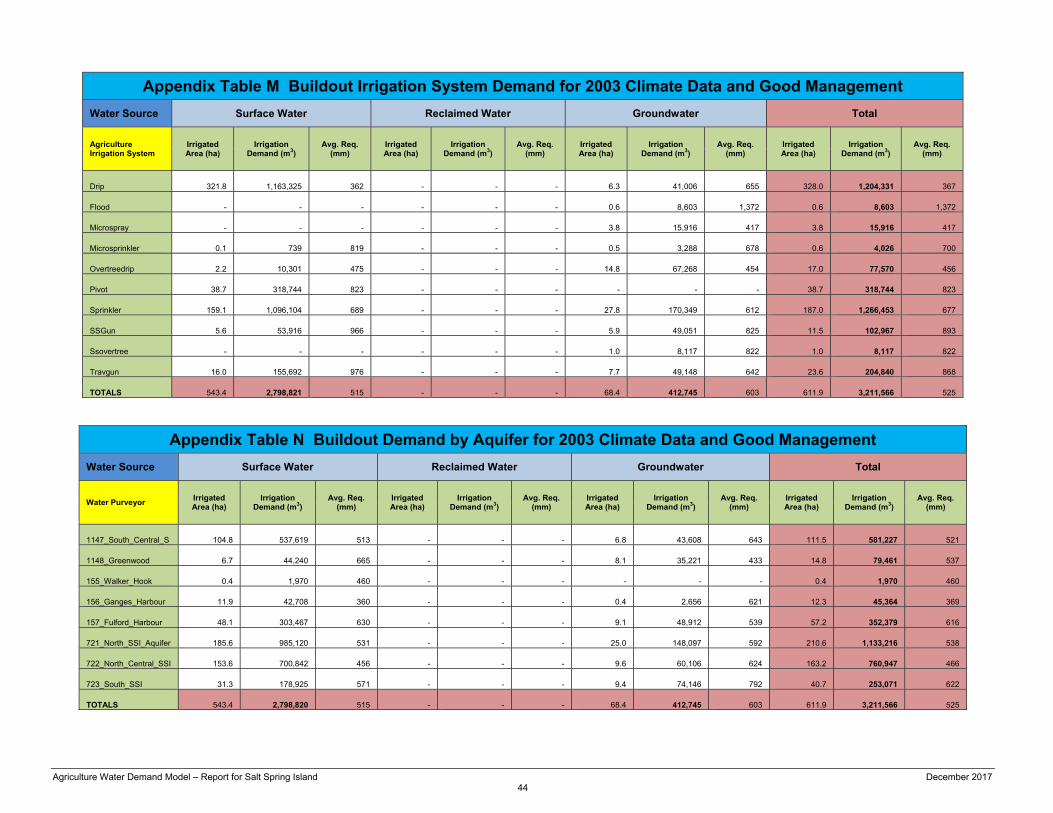
Agriculture Water Demand Model – Report for Salt Spring Island December 2017 44
Appendix Table M Buildout Irrigation System Demand for 2003 Climate Data and Good Management
Water Source Surface Water Reclaimed Water Groundwater Total
Agriculture Irrigation System
Irrigated Area (ha)
Irrigation Demand (m3)
Avg. Req. (mm)
Irrigated Area (ha)
Irrigation Demand (m3)
Avg. Req. (mm)
Irrigated Area (ha)
Irrigation Demand (m3)
Avg. Req. (mm)
Irrigated Area (ha)
Irrigation Demand (m3)
Avg. Req. (mm)
Drip
321.8
1,163,325
362
-
-
-
6.3
41,006
655
328.0 1,204,331
367
Flood
-
-
-
-
-
-
0.6
8,603
1,372
0.6 8,603
1,372
Microspray
-
-
-
-
-
-
3.8
15,916
417
3.8 15,916
417
Microsprinkler
0.1
739
819
-
-
-
0.5
3,288
678
0.6 4,026
700
Overtreedrip
2.2
10,301
475
-
-
-
14.8
67,268
454
17.0 77,570
456
Pivot
38.7
318,744
823
-
-
-
-
-
-
38.7 318,744
823
Sprinkler
159.1
1,096,104
689
-
-
-
27.8
170,349
612
187.0 1,266,453
677
SSGun
5.6
53,916
966
-
-
-
5.9
49,051
825
11.5 102,967
893
Ssovertree
-
-
-
-
-
-
1.0
8,117
822
1.0 8,117
822
Travgun
16.0
155,692
976
-
-
-
7.7
49,148
642
23.6 204,840
868
TOTALS
543.4 2,798,821
515
-
-
-
68.4 412,745
603
611.9 3,211,566
525
Appendix Table N Buildout Demand by Aquifer for 2003 Climate Data and Good Management
Water Source Surface Water Reclaimed Water Groundwater Total
Water Purveyor Irrigated Area (ha)
Irrigation Demand (m3)
Avg. Req. (mm)
Irrigated Area (ha)
Irrigation Demand (m3)
Avg. Req. (mm)
Irrigated Area (ha)
Irrigation Demand (m3)
Avg. Req. (mm)
Irrigated Area (ha)
Irrigation Demand (m3)
Avg. Req. (mm)
1147_South_Central_S
104.8
537,619
513
-
-
-
6.8
43,608
643
111.5 581,227
521
1148_Greenwood
6.7
44,240
665
-
-
-
8.1
35,221
433
14.8 79,461
537
155_Walker_Hook
0.4
1,970
460
-
-
-
-
-
-
0.4 1,970
460
156_Ganges_Harbour
11.9
42,708
360
-
-
-
0.4
2,656
621
12.3 45,364
369
157_Fulford_Harbour
48.1
303,467
630
-
-
-
9.1
48,912
539
57.2 352,379
616
721_North_SSI_Aquifer
185.6
985,120
531
-
-
-
25.0
148,097
592
210.6 1,133,216
538
722_North_Central_SSI
153.6
700,842
456
-
-
-
9.6
60,106
624
163.2 760,947
466
723_South_SSI
31.3
178,925
571
-
-
-
9.4
74,146
792
40.7 253,071
622
TOTALS
543.4 2,798,820
515
-
-
-
68.4 412,745
603
611.9 3,211,566
525