Estimation of Water Demand in Developing … of Water Demand in Developing Countries - An Overview...

Estimation of Water Demand in Developing Countries - An Overview

Céline Nauges National Institute for Research in Agriculture (INRA) and Toulouse School of Economics,

France

Dale Whittington Department of City and Regional Planning, University of North Carolina (USA)

Preliminary draft – Please do not quote

1

2

cussions.

1. Introduction

Water resource planners are facing increasing challenges due to the growing hydrologic

variability brought about by climate change. Also, incomes and populations of megacities are

both growing, placing new pressures on water resources in many places. Hence, water

resource managers need a much better understanding of household demand to manage water

systems and we believe a review of what we know and do not know about household water

demand in developing countries is timely.

On the one hand, household water demand has been extensively analyzed in developed

countries, in particular to provide price and income elasticities measures. In these countries,

almost all households get a connection to the water network and tap water is usually the

unique source of drinking water, in general of satisfactory quality. These characteristics make

the estimation of a water demand function relatively straightforward. The main

methodological issue that has been extensively discussed is the one related to the non-linearity

of the pricing scheme which may cause endogeneity bias at the estimation stage. On the other

hand, estimation of water demand functions in less developed countries (LDCs) remains

scarce. One main reason is that the conditions of water access vary in general across

households, which makes almost impossible an analysis of water demand based on aggregate

data and requires well-designed surveys.1 Households in LDCs usually have the choice

among a set of water sources, including piped and non-piped sources with different

characteristics and levels of services (price, distance to the source, quality, reliability, etc.).

Water is thus a heterogeneous good in these countries, contrary to what is usually the case in

developed countries (Mu et al., 1990). Finally, getting water from non-tap sources outside the

house involves collection costs that need to be taken into account. Carefully designed

household surveys are thus needed, and a significant amount of information on water services

has to be collected in order to allow for consistent water demand analysis. See also Mu et al.

(1990) for related dis

In this paper we discuss empirical issues including data requirement and methodological

problems that empirical researchers may face when estimating water demand in developing

countries.

1 Most analyses made in industrialized countries have been based on aggregate consumption data provided by water utilities (usually from records which the water utility maintains for billing purposes).

2. Estimation of water demand – A brief literature overview

Water demand estimation in developed countries has been at the core of many empirical

papers, starting with the work of Gottlieb (1963) and Howe and Linaweaver (1967). Studies

have been made in a large set of countries including Canada (Kulshreshtha, 1996), Denmark

(Hansen, 1996), France (Nauges and Thomas, 2000), Spain (Martínez-Espiñeira, 2002),

Sweden (Höglund, 1999), and above all the US (Foster and Beattie, 1979; Agthe and Billings,

1980; Chicoine et al., 1986; Nieswiadomy and Molina, 1989; Hewitt and Hanemann, 1995;

Pint, 1999; Renwick and Green, 2000). For comprehensive reviews, see Hanemann (1998),

Arbués-Gracia et al. (2003), or Dalhuisen et al. (2003).

In almost all studies, the water demand function is specified as a single demand equation for

water provided at the tap. Such an approach implicitly assumes that there is no substitute

available for water.2 Water quality as well as quality of the water supply service are not

controlled for, in general (for the main reason that there is not much variation in terms of

service quality across distribution units). The focus instead has been on the estimation of price

elasticity and the measurement of the impact of socioeconomic characteristics (income

mainly) on household water demand. The main methodological issues that have been

discussed all along is the choice of marginal price versus average price and price endogeneity

when households face a non-linear pricing scheme. If theory advocates the use of marginal

price (the price of the last cubic meter), average price (computed as total bill divided by total

consumption) has however often been preferred. Authors considering average price argue that

households are rarely well informed on the price structure and are thus more likely to react to

average price than to marginal price. To control for endogeneity, the instrumental variables

(IV) approach has been commonly used in the water demand as well as in the labor supply

and energy demand literature (Agthe et al. 1986; Deller et al. 1986; Nieswiadomy and Molina

1988, 1989). The use of instruments for the price variable (in a two-stage least squares

framework) allows to get unbiased estimates of the price coefficient in the demand equation.

The main drawback of this approach though, is that the interpretation of the price coefficient

as a price elasticity is conditional on the household remaining within the observed block of

consumption (Olmstead et al., 2007). The (only) theoretically consistent approach so far is the

2 The only exception is Hansen (1996) who considers water and energy prices in the demand function for water.

3

two-step approach describing the choice of the block (first step) and the choice of

consumption inside the block (second step), see Burtless and Hausman (1978) and Hewitt and

Hanemann (1995) for an application to the water sector.3

Household water use in developing countries has also been the focus of numerous articles, but

empirical evidence regarding factors driving water demand in these countries is still scarce.

Most studies on household water use have been under the form of contingent valuation studies

to derive willingness-to-pay for getting a house connection to a piped water network or, more

generally, improved water services (see among others Whittington et al. 1990a and

Whittington et al. 2002); and hedonic price studies to infer the valuation of a piped connection

through observations of house prices (see among others North and Griffin 1993, Daniere

1994, or Komives 2003 for a review). In this article, we will focus our attention on articles

which provide estimates of the water demand function for households in developing countries.

We will not comment on the earliest investigations of water demand that have basically used

the standard approach from the literature on industrialized countries (Inter-American

Development Bank, 1985a, b, c; Katzman, 1977; Hubbell, 1977) but instead on studies that

have tried to account for the specificities of water demand in developing countries. Our

purpose is to discuss the various empirical issues that have been encountered and the way

authors have addressed them. We will then review and compare the most important outcomes

of this set of articles.

3. Discussion of empirical issues

3.1. Underlying theoretical model

The water demand function for households is usually specified as an equation linking water

consumption q (the dependent variable) to water price (p) and a vector of demand shifters (x)

(household characteristics, weather conditions, house equipment) to control for heterogeneity

of preferences and outside variables affecting water demand:

( , )q f p u= x +

. (1)

3 Again, this approach remains theoretically appealing as long as households are aware of the pricing scheme.

4

The error term u is added to this relationship to account for unobservables and/or

measurement errors in variables. In most cases, function f is chosen to be linear in the

parameters.

When working on data from industrialized countries, authors commonly assume that this

demand function derives from the maximisation of household’s utility subject to a budget

constraint, under the assumption that water is a homogeneous good that has no direct

substitute or complement. In LDCs, the underlying theoretical model is described slightly

differently: water demand is usually assumed to be deriving from a model in which the

household is considered a joint production and consumption unit (see Berhman and

Deolalikar 1998 for description of such demand models).4 This is for the main reason that

demand for water can be regarded as a derived demand for an input to produce health (since

water consumption may have health consequences) and, as a consequence, health enters

household’s utility, along with consumption goods, leisure time, and other household’s

characteristics such as education. This preference function is then maximised subject to a

time-income constraint and a set of production functions. For related discussions, see Acharya

and Barbier (2002) or Larson et al. (2006).

3.2. Multiple sources

Households in LDCs may face a choice set of sources. This choice set can include water

sources as diverse as in-house tap connections, public or private wells, public or (someone

else’s) private taps, water vendors or resellers, tank trucks, water provided by neighbours or

water collected from rivers, streams or lakes. The choice set as well as the conditions of

access can vary significantly across households. We distinguish three main cases: (1) rural

areas – where piped distribution networks are often rare; (2) the formal parts of large cities

where piped networks are common, but many people may not be connected for a variety of

reasons, and (3) urban slums, which are very heterogeneous. Quality, reliability and

conditions of access (distance to get to the source, price) usually vary across sources, making

water a heterogeneous good.

4 In this setting, production and consumption are not assumed to be separable (separability condition may not hold if the nature of one’s occupation and one’s productivity directly interact with one health and nutrition).

5

Households may rely on a unique source or combine water from different sources. The fact

that some households utilize more than one source may indicate either that their use of a

particular convenient source is rationed (implying that additional water must be taken from an

alternative source), or that it is relatively cheap to take some water but not all from a

particular source (e.g. the household has limited capacity to haul cheap water from a given

source, and obtain the rest more expensively from another source); or that water from

different sources are used for different purposes (drinking, bathing, cleaning, etc.).

When households rely on a unique source or when water use comes primarily from one

source, a demand equation for water from that particular source can be estimated from data on

the sub-sample of households using that source: among other examples, Rizaiza (1991)

estimates separately demand equations for Saudi Arabian households with a private

connection and for households supplied with tankers; Crane (1994) specifies separate demand

equations for Indonesian households supplied by water vendors and for households relying on

hydrants; David and Inocencio (1998) on data from the Philippines estimate separate demand

equations for households supplied by water vendors and for households owning a private

connection; Rietveld et al. (2000) and Basani et al. (2007) estimate the water demand

equation for households with a piped connection. In some cases (Crane 1994, David and

Inocencio 1998), dummy variables are introduced in single demand equations to control for

possible use of extra sources.

Strand and Walker (2005) and Larson et al. (2006) distinguish only between piped and non-

piped water, i.e. they consider non-piped water as a homogeneous good, whatever the source

it comes from. In Nauges and Strand (2007), a single equation for non-tap water is also

estimated for households in Central American cities, but source-specific coefficients (in

particular for the price elasticity) are allowed in the demand model.

Finally, estimates of a demand function pooling data from piped and non-piped water sources

are reported in Strand and Walker (2005), using data from Central American cities. These

authors reject the null hypothesis of poolability of the data for piped and non-piped

households. The latter suggests that the homogeneity assumption for water from different

sources is likely to be a too strong assumption in most cases, in particular when comparing

piped and non-piped water.

6

The estimation of (single) source-specific demand equations provides insight on variables

driving water use from that particular source, such as its own price, quality and accessibility.

This approach does not allow to measure substituability/complementarity between water from

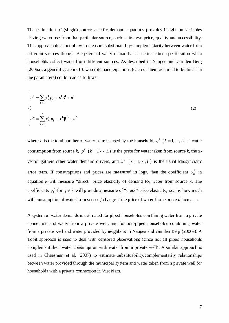
different sources though. A system of water demands is a better suited specification when

households collect water from different sources. As described in Nauges and van den Berg

(2006a), a general system of L water demand equations (each of them assumed to be linear in

the parameters) could read as follows:

1 1 1

1

1

L

k kk

LL L L

k kk

q p

q p

γ

γ

=

=

⎧= + +⎪

⎪⎪⎨⎪⎪ = + +⎪⎩

∑

∑

1 1

L L

x β

x β

u

u

L

(2)

where L is the total number of water sources used by the household, is water

consumption from source k,

kq ( )1, ,k =

kp is the price for water taken from source k, the x-

vector gathers other water demand drivers, and

( 1, ,k = )L

ku ( )1, ,k = L is the usual idiosyncratic

error term. If consumptions and prices are measured in logs, then the coefficient kkγ in

equation k will measure “direct” price elasticity of demand for water from source k. The

coefficients jkγ for j k≠ will provide a measure of “cross”-price elasticity, i.e., by how much

will consumption of water from source j change if the price of water from source k increases.

A system of water demands is estimated for piped households combining water from a private

connection and water from a private well, and for non-piped households combining water

from a private well and water provided by neighbors in Nauges and van den Berg (2006a). A

Tobit approach is used to deal with censored observations (since not all piped households

complement their water consumption with water from a private well). A similar approach is

used in Cheesman et al. (2007) to estimate substituability/complementarity relationships

between water provided through the municipal system and water taken from a private well for

households with a private connection in Viet Nam.

7

All the above discussion has concerned the specification of the demand equation for water

from some source, conditional on that source being chosen.

3.3. Simultaneity of choice between source and quantity

The simultaneity between choice of water source and choice of quantity was first

acknowledged by Whittington et al. (1987). These authors argue that a complete set of water

demand relationships should include models of both water source choice and the quantity of

water demanded. If not taken into account, the simultaneity in both decisions could lead to

biased estimates of the demand parameters. In particular, if some unobserved variables affect

both the choice of water source(s) and the quantity of water used, then estimated parameters

could suffer from selection bias (Heckman, 1979). This issue was acknowledged by several

authors and two-step Heckman procedure for selection bias correction was applied by, among

others, Larson et al. (2006) on data from Madagascar, Nauges and van den Berg (2006a) on

data from Sri Lanka, Basani et al. (2007) on data from Cambodia, Cheesman et al. (2007) on

data from Viet Nam and Nauges and Strand (2007) on data from Central American cities.

In most cases (Larson et al. 2006, Nauges and van den Berg 2006a, Basani et al. 2007), the

first stage involves estimation of a probit model for use of a private connection versus reliance

on non-tap sources. In Cheesman et al. (2007), a probit model is estimated to control for piped

households combining water from their private connection with water from a private well. In

Nauges and Strand (2007), the first stage involves estimation of a multinomial logit model

(MNL) for choice of the primary non-tap water source. Selectivity correction terms are

computed from the estimation of the discrete choice models and added linearly to the demand

equations. Statistical significance of these correction terms indicates presence of selectivity

bias.5

The first-step estimation is also interesting in itself since it indicates the variables that affect

household’s choice of water source. Mu et al. (1990) argue that the discrete choice model

offers a more promising approach for developing predictions of the aggregate number of

households which will choose a new source than the traditional (linear) demand model. Some

other articles have focused only on household’s choice of water source and will be discussed

5 See Heckman (1979) [resp. Lee (1983) and Dubin and McFadden (1984)] for computation of correction terms when a probit [resp. a MNL] is used in the first estimation stage.

8

here as well: this includes Madanat and Humplick (1993) on data from Pakistan, Hindman

Persson (2002) on data from The Philippines and Briand et al. (2006) on data from Senegal.

Authors generally agree that both source attributes (i.e., price, distance to the source, quality,

reliability) and household characteristics (income, education, size and composition) should

enter the choice model. Source attributes account for heterogeneity in water from different

sources while household characteristics account for difference in tastes, opportunity cost of

time, and perception of health benefits from improved water.

The most frequent specifications for source choice models are the probit model and the

multinomial logit (MNL) model. The latter has been used to describe either the primary

source of water chosen by households (Mu et al. 1990, Nauges and Strand 2007) or the water

source which is chosen for a specific use such as drinking, bathing or cooking (Madanat and

Humplick 1993, Hindman Persson 2002).6 The MNL model relies on the assumption that

alternatives are exclusive and rule out the possibility of combination of sources. In Briand et

al. (2006), a bivariate probit model is estimated to describe households’ decision to rely on a

private connection or/and household’s decision to use public standpipes.

A complex issue which has not been really addressed in the above-cited articles, is the

question of the choice set for each household. In peri-urban areas in particular, it may be the

case that all households do not have access to all possible water sources (for example, they

may not have the possibility to get a private connection because their living area is not

supplied by the municipal water network). Hindman Persson (2002) assumes that the choice

of household’s location in the city determines the set of available sources for each household.

3.4. The cost of water

Price

Piped water in the developing world is often charged following an increasing block pricing

scheme, thus leading to the same endogeneity issues as the ones discussed in the water

6 Hindman Persson (2002) estimates a probit model but argues that a nested conditional logit model would be better suited. Madanat and Humplick (1993) estimate a two-level sequential choice model to distinguish between the decision to get a private connection and the choice of non-tap sources.

9

demand literature in industrialized countries. The same techniques are consequently used to

estimate water demand in LDCs under complex pricing: David and Inocencio (1998), Strand

and Walker (2005), and Nauges and van den Berg (2006a) implement an IV approach to

control for endogeneity of price; Rietveld et al. (2000) apply the discrete/continuous model

along the lines of Hewitt and Hanemann (1995). Identification of price elasticity may be

difficult though in some cases (or even impossible), in particular when data come from

households surveys made in a single city or village. In such cases, there is little cross-

sectional variation in the policy-relevant variables such as connection costs, tariff and levels

of service. For example, Larson et al. (2006) exclude the price of water from their analysis of

water demand in Fianarantsoa (Madagascar) due to no cross-sectional variation in this

variable (all surveyed households face the same price schedule).

As for non-piped water, the situation varies across places and across sources: water can be

distributed free of charge, it can be charged at the bucket, etc. When a price for water exists,

then it is usually quite easy to compute a per unit price for each household and each source. If

households surveyed get water from different non-tap sources, or from different locations,

some cross-sectional variation will likely be observed in the data. The price of non-piped

water has been considered exogenous in all studies except in David and Inocencio (1998).

These authors argue that the price of vended water in metro Manila (The Philippines) may be

endogenous because price is determined by demand and supply factors. More precisely, due

to the fragmented nature of the water vending market, household decisions of water demand

are likely to influence its price.

Even if free of charge, the collection of water from non-piped sources usually involves costs

for hauling water from distant sources.

Collection costs

Use of water distributed from non-tap sources usually involves hauling time that comprises

time to go to the source, time to wait at the source, and time to haul water. Surveys often

gather information on distance or time needed to collect the water, more rarely is information

provided on who in the household is in charge of collecting water. The latter is probably the

main reason why time cost is usually not translated into a pecuniary collection cost: among

other examples, Larson et al. (2006) consider roundtrip walking time to water source and

10

waiting time at the source; David and Inocencio (1998) use distance from source in meters as

an explanatory variable in the demand model; Strand and Walker (2005) consider hauling

time per unit of water consumed. In order to convert time cost into monetary cost, one needs

to measure the opportunity cost of time of the person in charge of water collection.

Conceivably, one could convert collection time into collection costs using a proxy for the

unitary cost of time. The latter may be difficult to evaluate though, in particular if one does

not know who is in charge of collecting the water. Whittington et al. (1990b) are among the

only authors to provide some empirical evidence about the pecuniary cost of collecting water

from non-tap sources. These authors develop two approaches based on discrete choice theory

to estimate the value of time spent collecting water and illustrate their application using data

from Ukunda, Kenya. Their results indicate that the value of time for those households relying

on non-tap sources (kiosks, vendors or open wells in this village) is at least 50% of the market

wage rate and likely to be near the market wage rate for unskilled labor.7 Nauges and Strand

(2007) are the only authors to transform hauling time into corresponding pecuniary time cost.

They use the average hourly wage in the household as the shadow cost of time, but

acknowledge that this approximation may overestimate actual costs if the hauling is

performed by a child. Finally, Mu et al. (1990) argue that in places where the queue time

varies significantly over the course of the day, the collection time could be determined

endogeneously.

Capital investments for coping with unreliable supply

In response to deficiencies in the water supply system, households may invest in coping

strategies, i.e., they may incur fixed costs in the form of investments in alternate supply

sources and/or storage facilities. For example, households may buy a storage tank in order to

mitigate the reliability and pressure problems that may be associated with private house

connections, or they may invest in pumping equipment if relying on well water.

The use of a storage tank or capacity of the water reservoir is controlled for in the demand

equation estimated by Crane (1994), Nauges and van den Berg (2006a) and Cheesman et al.

(2007). Crane (1994) argues that use of a storage tank (and its capacity) could be endogenous 7 These figures were much higher than the ones recommended by the Inter-American Development Bank at the time: for the IADB, time savings should be valued at 50% of the market wage rate for unskilled labor (Whittington et al. 1990b).

11

in the demand model as the reservoir investment decision was certainly codetermined with the

expected need for water.

3.5. Quality of water and quality of service

Since water quality and reliability may vary from one source to another, such variables should

be included in the demand models (as well as in models describing source choice). This

includes opinion variables about taste, smell, color of water, hours of water availability and

potential pressure problems (for piped water). Most of the time these variables are provided

by households themselves and may be subject to misreporting. The variables measuring

household’s opinion (or perception) about water quality should also be used with caution

since they may cause endogeneity in the demand model. For example, households who

suffered from water-related diseases in the past may believe that water is less safe than

healthy households and hence have different behaviour regarding water use (Nauges and van

den Berg 2006b). In order to avoid any such endogeneity bias, one could use average opinion

(on water quality) of households living in the same neighbourhood or relying on the same

water source, where the average would be computed without considering the opinion of the

household under consideration (Briand et al. 2006).

3.6. Summary of data and estimation issues

Data problems

a) Data on water use and price for (metered) households with a private connection are

usually recorded from water bills that have to be shown by households. Metered water use

data may be poor in some places though because pressures are intermittent, and meters may

not provide accurate readings. This is because when the water utility does not supply 24-hour

service, air gets into the pipes and the meter can register water passing through when it is

really just air.8 The importance of this basic data problem is often not well-appreciated or is

simply ignored.

8 Also, because water prices are so low in many places, and corruption is high, water utilities have no incentive to keep meters in good working order. So they are not replaced on a timely basis. The end result of all this is that in many cases no one know how much water a household is using – not the utility, not the household, and certainly not the researcher.

12

b) When surveys are made in a single village or town, there is usually not enough

cross-sectional variation in the conditions of access to water (price, quality and reliability of

water). This lack of cross-sectional variation may impede identification of parameters of

interest such as the price elasticity of water demand. One may overcome this problem by

combining revealed and stated preference data, which results in respondents each having

multiple observations (and above all multiple water use observations for different

(hypothetical) levels of prices). For applications of this approach to household water demand,

see Acharya and Barbier (2002) and Cheesman et al. (2007).

c) Data on consumption and price for households relying on non-piped sources are

usually based on self-reported information (households are usually asked to report the number

of buckets that they get every day), so there is likely to be substantial measurement error. If

consumption data are used as dependent variables, random measurement errors leads to

imprecise parameter estimates (the measurement error may however not always be random

and may depend on the education of the household’s head for example). If price data are used

as right-hand-side variables, then this may cause bias in the parameter estimates.

d) Data on consumption, price, service quality are typically recorded over short

reference periods (a month), which may not be representative of household’s normal

behaviour (in the event of a wedding or ceremony, households may store water). Also, service

quality and quality of water may vary across seasons.

e) Information on income may be difficult to gather in some places. Whittington et al.

(1990a) stated “the principal investigators and the enumerators had agreed that it was not

possible to obtain accurate information on household income through interviews […]. As a

substitute, the enumerator recorded a series of observations about the construction of the

house itself, such as whether the house was painted, whether the roof was straw or tin, and

whether the floor of the house was dirt or cement.” Basani et al. (2007) use household

expenditure as a proxy for income, arguing that households surveyed are more likely to

undestate their incomes than overstate their expenditure (Deaton, 1997).

Estimation issues

13

The specificities of water demand in developing countries complicates the estimation of the

water demand function:

f) Households usually face a set of possible choices in terms of water sources but this

set may vary across households. The choice of which water source to rely on and the quantity

of water used are likely to be determined simultaneously. This implies the specification of a

model describing both the choice of the source and quantity of water used. Until now, probit

and multinomial logit models have been used most often. The probit model has been used to

model the decision of households to get or not a tap connection. The multinomial logit has

proven useful to describe household’s choice of primary source of water or household’s

choice of water source for a specific usage. The multinomial logit considers choices between

exclusive alternatives and relies on the assumption of independence from irrelevant

alternatives (IIA). If one wants to model household’s choice of water sources, allowing for

combination of sources, then multivariate probit or nested logit models should be the

preferred alternative. In the multivariate probit setting, households are assumed to make

several decisions, each between two alternatives. In the nested logit setting, alternatives are

grouped into sub-groups, which allows the variance to differ across the groups while

maintaining the IIA assumption within the groups. The nested logit specification can be seen

as a two-(or more) level choice problem. See Greene (2003, Ch. 21) for greater details on

these models.

g) Households may combine water from different sources. Aggregation of water from

different sources and estimation of a single demand equation for water may provide

misleading results. Estimation of a system of demand equations is better suited and allows the

measurement of direct and cross-price elasticities. To control for censoring of observations in

a system of equations, one could refer to the approach developed by Shonkwiler and Yen

(1999).

h) Water from different sources usually have different characteristics in terms of price,

conditions of access, reliability and quality. These characteristics should be controlled for in

the model describing household’s choice of water source and household’s demand for water.

Since data on service quality and reliability are based on household’s opinion, they could

suffer from endogeneity or be measured with some error.

14

i) Piped water is commonly sold through a non-linear pricing scheme and price of

water may be endogenous in the water demand equation. Estimation techniques like

instrumental variables or discrete/continuous choice approaches (Burtless and Hausman 1978,

Hewitt and Hanemann 1995) should be used. Again, the latter is appealing as long as

households are aware of the pricing scheme.

j) The price of non-piped water may be endogenous in some cases, in particular if

water is re-sold by vendors who may change the price depending on demand and supply

conditions.

k) Hauling time may be endogenous if the time to queue at the source varies during the

day.

l) The decision of households to engage in coping strategies such as buying a storage

tank or investing in pumping equipment may be determined simultaneously with the choice of

water source and the quantity of water used, making this variable endogenous.

4. Main results from estimation of water demand equations

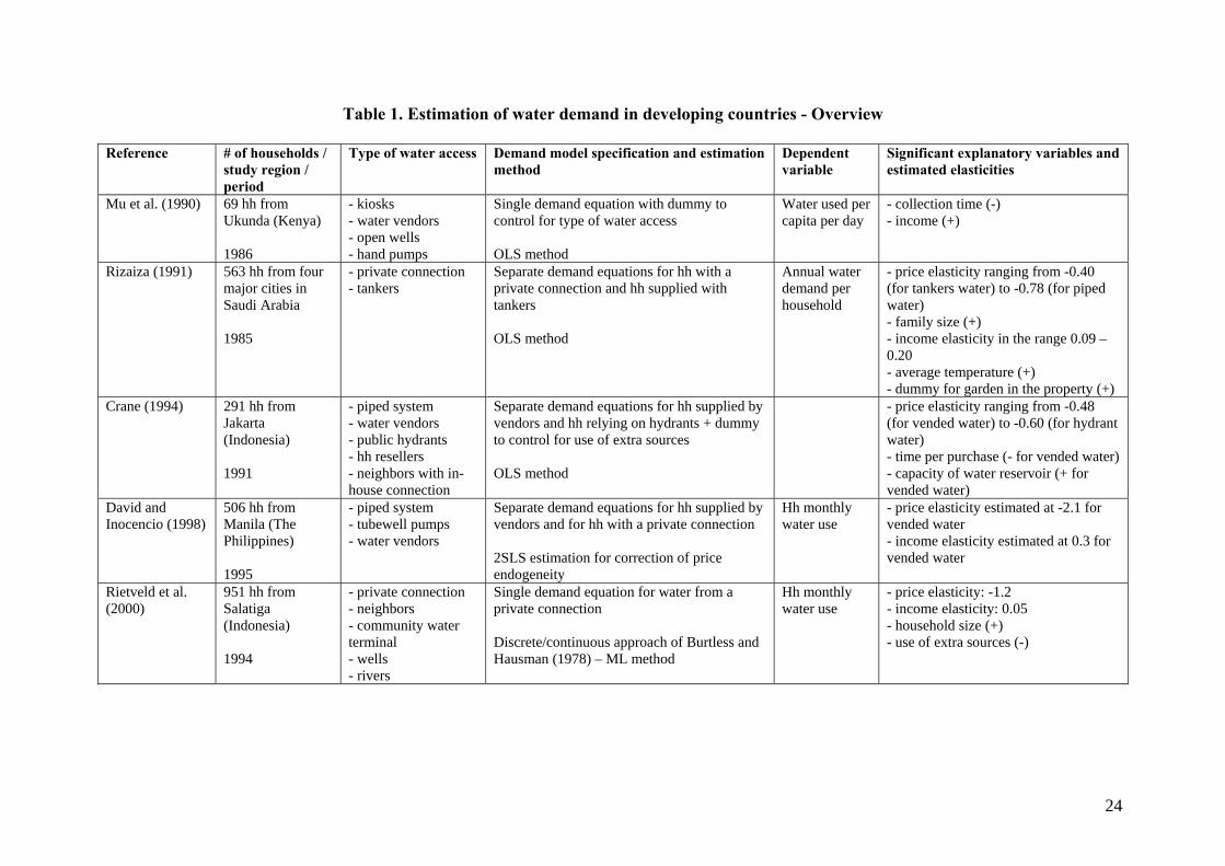
The main characteristics of each above-cited study (number of households, study area, time

period), type of water access of surveyed households, econometric approach used for

estimation of water demand, and main estimation results are shown in Table 1.

The studies recorded in the present article have used data from various regions in the world:

Central America (El Salvador, Guatemala, Honduras, Nicaragua, Panama, Venezuela), Africa

(Kenya, Madagascar) and Asia (Cambodia, Indonesia, The Philippines, Saudi Arabia, Sri

Lanka, Viet Nam), and cover a twenty-year time span (the earliest survey dates back to 1985

while the most recent one has been made in 2006). Despite heterogeneity in places and time

periods, authors seem to agree on the inelasticity of water demand in LDCs, with most

estimates in the range -0.3 to -0.6. Only two studies find evidence of an elastic water demand:

David and Inocencio (1998) using data from The Philippines estimate price elasticity for

vended water at -2.1 and Rietveld et al. (2000) estimate price elasticity for piped water at -1.2

using data from Indonesia. Interestingly, Rietveld et al. (2000) are the only authors to use the

discrete-continuous model first proposed by Burtless and Hausman (1978) and transposed to

15

the water demand literature by Hewitt and Hanemann (1995). These authors had used this

approach to estimate water demand in Texas and price elasticity was estimated at -1.6. This

figure was above (in absolute value) most elasticities that had been estimated in developed

countries (Espey et al. 1997 report an average of -0.51 for industrialized countries). The price

elasticity estimated by David and Inocencio (1998) should be regarded with some caution

since alternative estimation techniques used on the same data (by the same authors) seem to

provide very different price elasticities. All in all, and based on the existing studies for

household water use in LDCs, estimated price elasticity for these households seem to be in the

range of price elasticities estimated in industrialized countries.

Two recent studies (Nauges and van ben Berg 2006a and Cheesman et al. 2007) have shown

new insights regarding price elasticity in LDCs. By choosing to estimate system of water

demands, they have shown that water from different sources may be used as substitutes. More

importantly, these authors report that piped households relying on piped water only are less

sensitive to price changes than piped households who complement their water consumption

from the tap with water from a private well.

For households relying on non-tap water sources, collection time is found to have a significant

negative impact on quantity of water consumed, as expected.

In almost all studies, income elasticity (or expenditure elasticity) is found to be quite low,

most often in the range 0.1 – 0.3.

Household size, as expected, is found to be significant in most studies. When the dependent

variable is total household consumption, larger households are found to have larger water use.

When the dependent variable is per capita consumption, scale effects are confirmed, i.e., per

capita consumption decreases with the number of members in the household.

The presence of a storage tank is found to induce higher consumption in two studies (Nauges

and van den Berg 2006a and Cheesman et al. 2007). Also, piped water being available for

longer hours is found to increase water use by piped households (Nauges and van den Berg

2006). Variables measuring households’ opinion about water quality are not found significant

in general.

16

To account for potential selection bias, authors usually rely on the two-step Heckman

approach involving estimation of a discrete-choice model in the first step.9 As mentioned

before, some articles focus only on household’s choice of water source and will be discussed

here as well. This includes Madanat and Humplick (1993) on data from Pakistan, Hindman

Persson (2002) on data from The Philippines and Briand et al. (2006) on data from Senegal.

The discrete-choice approach has been used to describe household’s choice of primary water

source (Mu et al. 1990, Nauges and Strand 2007), or household’s choice of usage-specific

water sources (Madanat and Humplick 1993, Hindman Persson 2002), or household’s

decision to get or not a private connection (Larson et al. 2006, Nauges and van den Berg

2006a, Basani et al. 2007). Results from these models usually confirm that both source

characteristics and household’s characteristics have significant impact on source choice (see

Table 2). Source characteristics that are found to be significant drivers of household’s choice

are collection time or distance to the source (Mu et al. 1990, Hindman Persson 2002, Briand

et al. 2006), water price (Mu et al. 1990), piped water pressure level (Madanat and Humplick

1993), and opinions about taste and reliability of water (Nauges and van den Berg 2006a,

Briand et al. 2006). As for household characteristics, almost all studies find evidence that

income (or expenditure) and education level (or the ability of household’s head to read and

write) drive household’s choice of water source (Madanat and Humplick 1993, Hindman

Persson 2002, Briand et al. 2006, Larson et al. 2006, Nauges and van den Berg 2006a, Basani

et al. 2007, Nauges and Strand 2007). Mu et al. (1990) and Briand et al. (2006), using data

from Kenya and Senegal respectively, find evidence that household’s composition affects

choice of water source: in Ukunda (Kenya), households with more women are found to be

less likely to use vendors (and more likely to rely on water from wells and kiosks) because

more people are available in the household unit to carry water. In Dakar (Senegal), the

probability that households use water from the piped system increases if the household’s head

is a widow.

5. Conclusion [to be completed]

9 Even if the empirical evidence is rather limited, it is interesting to mention that no evidence for selection bias due to the choice of water sources was found in Nauges and van den Berg (2006a), Basani et al. (2007) and Cheesman et al. (2007).

17

This overview of empirical issues has shown that a careful analysis of households’ water

demand in LDCs requires a high level of information from the household. Things to

remember when designing a survey on water demand are:

a- Surveys should ideally be made in different cities/villages in order to have some cross-

sectional variation in conditions of water services, in particular price, connection fee, quality

and reliability of services.

b- In most cases, only data on sources that are actually used by the surveyed household are

available. Ideally, one should identify the complete set of sources available to the household

and gather information on time to walk to the source and time to wait at the source, price of

the water, possible rationing or constraints (opening hours, limited availability) and quality of

the water from each source (even if not used by the household). This is a prerequisite for

consistent estimation of household’s choice of water sources.

c- The measurement of hauling costs is not easy, in particular when one does not have

information on who is in charge of collecting water in the household. Information of the

persons in charge of collecting the water should be gathered.

d- There is no clear evidence that households who have a piped connection are aware of the

water pricing scheme. Whether or not households know the price of water is likely to depend

on factors such as the share of water bill in overall expenditure, the complexity of the water

pricing scheme, the frequency of billing, and the education level in the household. At the time

of the survey, interviewers should test households’ knowledge about their consumption and

water expenditure of the last period, and the pricing scheme. This issue has usually been

ignored in studies using data from developed countries.10

As a conclusion, we would also like to point out that there are important questions about

household water demand behaviour in developing countries that have not yet been addressed

or simply cannot be addressed with existing data. First, because most data set are cross-

sectional, dynamic analyses of water demand are not doable (by “dynamic” water demand, we

mean a water demand function in which consumption of the last period is included in the list

of covariates). Estimation of water demand in a dynamic framework is useful though, since it

provides measures of households’ responses to a changing environment on the long-run.

10 One exception is Gaudin (2006) which tests, on US data, if differences in the informational content of bills may affect the intensity with which consumers respond to price signals. She finds that price elasticity increases by 30% or more when price information is given on the bill.

18

Using aggregate data from France, Nauges and Thomas (2003) have shown that the “long-

run” price elasticity of water demand (that is the change in consumption following several

years of price increase) was significantly higher in magnitude than the “short-term” price

elasticity (i.e., price elasticity derived from the estimation of the traditional static demand

function). Such analyses have not been performed yet on LDCs.

Second, existing data do not allow us to measure how household water use would respond to

the establishment of dual networks (one for drinking and cooking, and the other for uses that

do not require such high quality water).

Third, welfare analysis following changes in the conditions of water supply for households in

LDCs remains a difficult question, in particular when piped water is charged following a

block-pricing scheme and when scenarios involve the connection to the piped network of

households that are currently without a connection. As discussed earlier, consistent estimation

of water demand under block pricing and the computation of the change in consumption

following a change in price is computationally difficult (for details, see Olmstead et al.,

2007). The other issue arises from the fact that it is difficult for the researcher to assess water

demand for piped water, for households who currently do not have a connection to the piped

network. The assumption that households without a piped connection will behave as

households who currently have one, is likely to be too strong in most cases, since there is

evidence that household’s own characteristics drive both their choice or access to specific

water sources and the quantity of water they use.

19

20

References

Acharya, G. and E. Barbier, 2002. “Using domestic water analysis to value groundwater recharge in the Hadejia-Jama’Are floodplain, northern Nigeria”. American Journal of Agricultural Economics 84: 415–26.

Agthe, D.E., and R.B. Billings, 1980. “Dynamic models of residential water demand.” Water Resources Research 16 (3): 476–480.

Agthe, D.E., R.B. Billings, J.L. Dobra, and K. Raffiee, 1986. “A Simultaneous Equation Demand Model for Block Rates”. Water Resources Research 22(1): 1-4.

Arbués-Gracia, F., García-Valiñas, M. A., and R. Martínez-Espiñeira, 2003. “Estimation of Residential Water Demand: A State of the Art Review”. Journal of Socio-Economics 32(1): 81-102.

Basani, M., J. Isham, and B. Reilly, 2007. “The Determinants of Water Connection and Water Consumption: Empirical Evidence from a Cambodian Household Survey.” World Development, forthcoming.

Behrman, J.R. and A.B. Deolalikar, 1988. Health and nutrition, in: J. Behrman and T. N. Srinivasan (eds) Handbook of Development Economics, Vol. I. pp. 633–711 (Amsterdam: Elsevier Science).

Briand, A., Nauges, C., and M. Travers, 2006. “Choix d’approvisionnement en eau des ménages de Dakar : une étude économétrique à partir de données d’enquête.” Working paper, LERNA-INRA (in French).

Briscoe, J., P. Furtado de Castro, C. Griffin, J. North, and O. Olsen., 1990. “Toward Equitable and Sustainable Rural Water Supplies: A Contingent Valuation Study in Brazil.” The World Bank Economic Review 4(2): 115-134.

Burtless, G., and J. Hausman, 1978. “The Effect of Taxation on Labour Supply: Evaluating the Gary Income Maintenance Experiment”. Journal of Political Economy 86(1): 103–130.

Cheesman, J., T. V. H. Son, et al. (2007). The economic value of household water in Buon Ma Thuot, Viet Nam. Managing groundwater in the Central Highlands of Viet Nam. Research Paper No 3. Canberra, The Australian National University.

Chicoine, D.L., Deller, S.C., and G. Ramamurthy, 1986. “Water demand estimation under block rate pricing: a simultaneous equation approach.” Water Resources Research 22(6): 859-863.

Crane, R., 1994. “Water Markets, Market Reform and the Urban Poor: Results from Jakarta, Indonesia”. World Development 22(1): 71-83.

Dalhuisen, J.M., R. Florax, H. De Groot, and P. Nijkamp, 2003. “Price and Income Elasticities of Residential Water Demand: A Meta-Analysis”. Land Economics 79(2): 292-308.

Daniere, A., 1994. “Estimating Willingness to Pay for Housing Attributes: An Application to Cairo and Manila”. Regional Science and Urban Economics 24:577-599.

David, C.C., and A.B. Inocencio, 1998. Understanding Household Demand for Water: The Metro Manila Case, Research Report, EEPSEA, Economy and Environment Program for South East Asia, available at http://web.idrc.ca/en/ev-8441-201-1-DO_TOPIC.html

Deaton, 1997 Deller, S.C., D.L. Chicoine and G. Ramamurthy, 1986. “Instrumental Variables Approach

to Rural Water Service Demand”. Southern Economic Journal 53(2): 333-346. Diakite, D., Semenov, A., and A. Thomas, 2006. “Social Pricing and Water Provision in

Cote d'Ivoire”. Working paper, LERNA-INRA (Toulouse), France. Dubin, J.A., and D.L. McFadden, 1984. “An econometric analysis of residential electric

appliance holdings and consumption.” Econometrica 52: 345-362.

Espey, M., Espey, J., and W.D. Shaw, 1997. “Price elasticity of residential demand for water: a meta-analysis”. Water Resources Research 33(6): 1369-1374.

Foster, H.S.J., and B.R. Beattie, 1979. “Urban residential demand for water in the United States.” Land Economics, 55(1): 43-58.

Gaudin, S., 2006. “Effect of Price Information on Residential Water Demand". Applied Economics 38(4): 383-93.

Gottlieb, M., 1963. “Urban domestic demand or water in the United States”. Land Economics 39 (2): 204–210.

Hanemann, W.M., 1998. “Determinants of Urban Water Use.” Chapter 2 in Urban Water Demand Management and Planning, edited by Duane Baumann, John Boland, and Michael Hanemann. New York: McGraw Hill, pp. 31–75.

Hansen, L.G., 1996. “Water and energy price impacts on residential water demand in Copenhagen”. Land Economics 72(1), 66–79.

Heckman, J., 1979. “Sample selection bias as a specification error.” Econometrica 47: 153-161.

Hewitt, J.A., and W.M. Hanemann, 1995. “A Discrete/Continuous Approach to Residential Water Demand under Block Rate Pricing”. Land Economics 71: 173-192.

Hindman Persson, T.H., 2002. “Household choice of drinking-water source in the Philippines”. Asian Economic Journal 16(4): 303-316.

Höglund, L., 1999. “Household demand for water in Sweden with implications of a potential tax on water use”. Water Resources Research 35(12): 3853-3863.

Howe, C.W., and F.P. Linaweaver, 1967. “The impact of price on residential water demand and its relationship to system design and price structure.” Water Resources Research 3(1): 13-32.

Hubbell, L. K., 1977. “The residential demand for water and sewerage service in developing countries: A case study of Nairobi”. Urban Reg. Rep. 77-14, Dev. Econ. Dep., World Bank, Washington D.C.

Inter-American Development Bank, Chile: Programa de agua portable rural: IV etapa, project report, Washington D.C., 1985a.

Inter-American Development Bank, Haiti: Second stage of the community health posts and rural drinking water supply program, project report, Washington D.C., 1985b.

Inter-American Development Bank, Honduras: Rural water supply program (III stage), project report, Washington D.C., 1985c.

Katzman, Martin 1977. "Income and Price Elasticities of Demand for Water in Developing Countries." Water Resources Bulletin 13: 47-55.

Komives, K., 2003. Infrastructure, Property Values, and Housing Choice: An Application of Property Value Models in the Developing Country Context. Ph.D. Dissertation, University of North Carolina, Department of City and Regional Planning.

Kulshreshtha, S.N., 1996. “Residential water demand in Saskatchewan communities: role played by block pricing system in water conservation”. Canadian Water Resources Journal 21(2): 139-155.

Larson, B., B. Minten and R. Razafindralambo, 2006. “Unravelling the linkages between the millennium development goals for poverty, education, access to water and household water use in developing countries: Evidence from Madagascar”. Journal of Development Studies 42(1): 22-40.

Lee, L.F., 1983. “Generalized econometric models with selectivity.” Econometrica 51: 507-512.Madanat, S. and F. Humplick, 1993. “A model of household choice of water supply systems in developing countries”, Water Resources Research 29: 1353–58.

Martínez-Espiñeira, R., 2002. « Residential water demand in the Northwest of Spain”. Environmental and Resource Economics 21(2): 161-187.

21

Mu, K., D. Whittington, and J. Briscoe, “Modeling village water demand behavior: A discrete choice approach,” Water Resources Research 26: 521-529.

Nauges, C., and J. Strand, 2007. “Estimation of Non-tap Water Demand in Central American Cities”. Resource and Energy Economics 29: 165-182.

Nauges, C., and A. Thomas, 2000. “Privately-operated water utilities, municipal price negotiation, and estimation of residential water demand: the case of France”. Land Economics 76(1): 68-85.

Nauges, C., and A. Thomas, 2003. “Long Run Study of Residential Water Consumption”, Environmental and Resource Economics 26(1): 25-43.

Nauges, C., and C. van den Berg, 2006a. “Household’s perception of water safety and hygiene practices: Evidence from Sri Lanka”, working paper LERNA.

Nauges, C., and C. van den Berg, 2006b. “Demand for Piped and Non-Piped Water Supply Services: Evidence from Southwest Sri Lanka”, working paper LERNA.

Nieswiadomy, M.L. and D.J. Molina, 1988. “Urban Water Demand Estimates under Increasing Block Rates”. Growth and Change 19(1): 1-12.

Nieswiadomy, M.L. and D.J. Molina, 1989. “Comparing Residential Water Demand Estimates under Decreasing and Increasing Block Rates Using Household Data”. Land Economics 65(3): 280-289.

North, J.H. and C.C. Griffin, 1993. “Water Source as a Housing Characteristic:Hedonic Property Valuation and Willingness to Pay for Water”. Water Resources Research 29: 1923-1929.

Olmstead, S.M., W.M. Hanemann, and R. N. Stavins, 2007. “Water Demand Under Alternative Price Structures”. Journal of Environmental and Economics Management 54: 181–198.

Pattanayak, S. J.C. Yang, D. Whittington, and B. Kumar, 2005. “Coping with Unreliable Public Water Supplies: Averting Expenditures by Households in Kathmandu, Nepal.” Water Resources Research 4(2), W02012, doi:10.1029/2003WR002443.

Pint, E., 1999. “Household responses to increased water rates during the California drought”. Land Economics 75(2): 246-266.

Renwick, M.E., and R. Green, 2000. “Do residential water demand side management policies measure up? An analysis of eight California water agencies”. Journal of Environmental Economics and Management 40(1): 37–55.

Rietveld P., J. Rouwendal and B. Zwart, 2000. “Block Rate Pricing of Water in Indonesia: An Analysis of Welfare Effects”. Bulletin of Indonesian Economic Studies 36(3): 73-92.

Rizaiza, O., 1991. “Residential water usage: A case study of the major cities of the western region of Saudi Arabia”. Water Resources Research 27(5).

Shonkwiler, J.S., and S.Y. Yen, 1999. “Two-Step Estimation of a Censored System of Equations”. American Journal of Agricultural Economics, 81: 972-982.

Strand, J., and I. Walker, 2005. “Water Markets and Demand in Central American Cities”. Environment and Development Economics 10(3): 313-335.

Whittington, D., J. Briscoe, and X. Mu, 1987. “Willingness to pay for water in rural areas: Methodological approaches and an application in Haiti”, Field report, 213, 93 pp., Water and Sanitation for Health Project, U.S. Agency for Int. Dev., Washington, D.C., Sept. 1987.

Whittington, D., Briscoe, J., Mu, X., and W. Barron, 1990a. “Estimating the Willingness to Pay for Water Services in Developing Countries: A Case Study of the Use of Contingent Valuation Surveys in Southern Haiti”. Economic Development and Cultural change 38(2): 293-311.

Whittington, D., and K. Choe, 1992. “Economic benefits available from the provision of improved potable water supplies,” WASH Technical Report No. 77.

22

Whittington, D., and M. Hanemann, 2006. “The Economic Costs and Benefits of Investments in Municipal Water and Sanitation Infrastructure: A Global Perspective”, working paper.

Whittington, D., Mu, X., and R. Roche, 1990b. “Calculating the Value of Time Spent Collecting Water: some Estimates for Ukunda, Kenya”. World Development 18(2): 226-280.

Whittington, D., Pattanayak, S.K., Jui-Chen, Y., and K.C. Bal Kumar, 2002. “Household Demand for Improved Piped Water Services: Evidence from Kathmandu, Nepal”. Water Policy 4(6): 531-556.

World Bank Water Demand Research Team, “The demand for water in rural areas: Determinants and policy implications,” The World Bank Research Observer Vol. 8: 47-70.

23

24

Table 1. Estimation of water demand in developing countries - Overview Reference # of households /

study region / period

Type of water access Demand model specification and estimation method

Dependent variable

Significant explanatory variables and estimated elasticities

Mu et al. (1990) 69 hh from Ukunda (Kenya) 1986

- kiosks - water vendors - open wells - hand pumps

Single demand equation with dummy to control for type of water access OLS method

Water used per capita per day

- collection time (-) - income (+)

Rizaiza (1991) 563 hh from four major cities in Saudi Arabia 1985

- private connection - tankers

Separate demand equations for hh with a private connection and hh supplied with tankers OLS method

Annual water demand per household

- price elasticity ranging from -0.40 (for tankers water) to -0.78 (for piped water) - family size (+) - income elasticity in the range 0.09 – 0.20 - average temperature (+) - dummy for garden in the property (+)

Crane (1994) 291 hh from Jakarta (Indonesia) 1991

- piped system - water vendors - public hydrants - hh resellers - neighbors with in-house connection

Separate demand equations for hh supplied by vendors and hh relying on hydrants + dummy to control for use of extra sources OLS method

- price elasticity ranging from -0.48 (for vended water) to -0.60 (for hydrant water) - time per purchase (- for vended water) - capacity of water reservoir (+ for vended water)

David and Inocencio (1998)

506 hh from Manila (The Philippines) 1995

- piped system - tubewell pumps - water vendors

Separate demand equations for hh supplied by vendors and for hh with a private connection 2SLS estimation for correction of price endogeneity

Hh monthly water use

- price elasticity estimated at -2.1 for vended water - income elasticity estimated at 0.3 for vended water

Rietveld et al. (2000)

951 hh from Salatiga (Indonesia) 1994

- private connection - neighbors - community water terminal - wells - rivers

Single demand equation for water from a private connection Discrete/continuous approach of Burtless and Hausman (1978) – ML method


- price elasticity: -1.2 - income elasticity: 0.05 - household size (+) - use of extra sources (-)

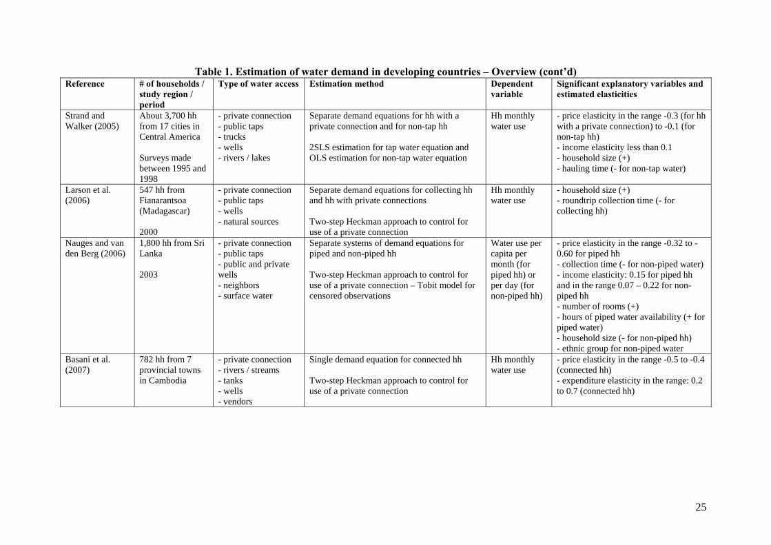
Table 1. Estimation of water demand in developing countries – Overview (cont’d) Reference # of households /


Type of water access Estimation method Dependent variable


Strand and Walker (2005)

About 3,700 hh from 17 cities in Central America Surveys made between 1995 and 1998

- private connection - public taps - trucks - wells - rivers / lakes

Separate demand equations for hh with a private connection and for non-tap hh 2SLS estimation for tap water equation and OLS estimation for non-tap water equation


- price elasticity in the range -0.3 (for hh with a private connection) to -0.1 (for non-tap hh) - income elasticity less than 0.1 - household size (+) - hauling time (- for non-tap water)

Larson et al. (2006)

547 hh from Fianarantsoa (Madagascar) 2000

- private connection - public taps - wells - natural sources

Separate demand equations for collecting hh and hh with private connections Two-step Heckman approach to control for use of a private connection


- household size (+) - roundtrip collection time (- for collecting hh)

Nauges and van den Berg (2006)

1,800 hh from Sri Lanka 2003

- private connection - public taps - public and private wells - neighbors - surface water

Separate systems of demand equations for piped and non-piped hh Two-step Heckman approach to control for use of a private connection – Tobit model for censored observations

Water use per capita per month (for piped hh) or per day (for non-piped hh)

- price elasticity in the range -0.32 to -0.60 for piped hh - collection time (- for non-piped water) - income elasticity: 0.15 for piped hh and in the range 0.07 – 0.22 for non-piped hh - number of rooms (+) - hours of piped water availability (+ for piped water) - household size (- for non-piped hh) - ethnic group for non-piped water

Basani et al. (2007)

782 hh from 7 provincial towns in Cambodia

- private connection - rivers / streams - tanks - wells - vendors

Single demand equation for connected hh Two-step Heckman approach to control for use of a private connection


- price elasticity in the range -0.5 to -0.4 (connected hh) - expenditure elasticity in the range: 0.2 to 0.7 (connected hh)

25

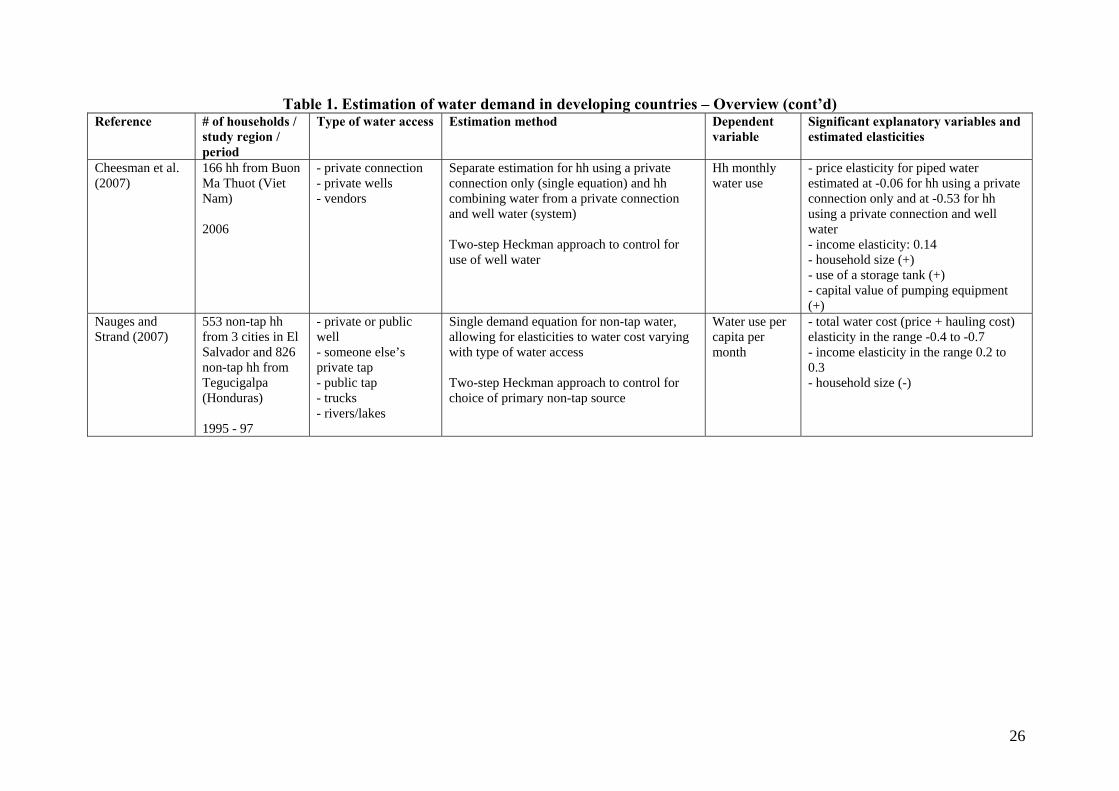
Table 1. Estimation of water demand in developing countries – Overview (cont’d) Reference # of households /


Type of water access Estimation method Dependent variable


Cheesman et al. (2007)

166 hh from Buon Ma Thuot (Viet Nam) 2006

- private connection - private wells - vendors

Separate estimation for hh using a private connection only (single equation) and hh combining water from a private connection and well water (system) Two-step Heckman approach to control for use of well water


- price elasticity for piped water estimated at -0.06 for hh using a private connection only and at -0.53 for hh using a private connection and well water - income elasticity: 0.14 - household size (+) - use of a storage tank (+) - capital value of pumping equipment (+)

Nauges and Strand (2007)

553 non-tap hh from 3 cities in El Salvador and 826 non-tap hh from Tegucigalpa (Honduras) 1995 - 97

- private or public well - someone else’s private tap - public tap - trucks - rivers/lakes

Single demand equation for non-tap water, allowing for elasticities to water cost varying with type of water access Two-step Heckman approach to control for choice of primary non-tap source

Water use per capita per month

- total water cost (price + hauling cost) elasticity in the range -0.4 to -0.7 - income elasticity in the range 0.2 to 0.3 - household size (-)

26

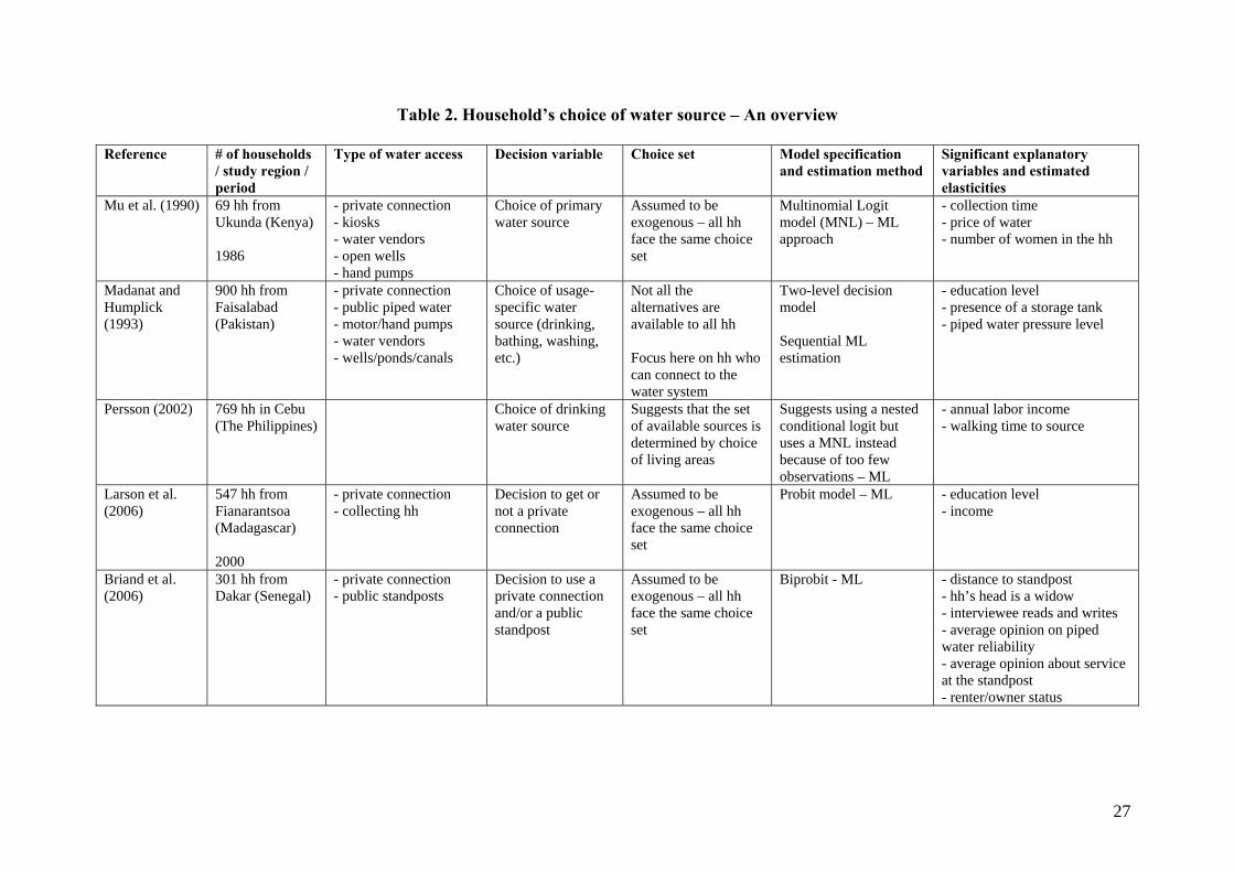
Table 2. Household’s choice of water source – An overview

Reference # of households / study region / period

Type of water access Decision variable Choice set Model specification and estimation method


Mu et al. (1990) 69 hh from Ukunda (Kenya) 1986

- private connection - kiosks - water vendors - open wells - hand pumps

Choice of primary water source

Assumed to be exogenous – all hh face the same choice set

Multinomial Logit model (MNL) – ML approach

- collection time - price of water - number of women in the hh

Madanat and Humplick (1993)

900 hh from Faisalabad (Pakistan)

- private connection - public piped water - motor/hand pumps - water vendors - wells/ponds/canals

Choice of usage-specific water source (drinking, bathing, washing, etc.)

Not all the alternatives are available to all hh Focus here on hh who can connect to the water system

Two-level decision model Sequential ML estimation

- education level - presence of a storage tank - piped water pressure level

Persson (2002) 769 hh in Cebu (The Philippines)

Choice of drinking water source

Suggests that the set of available sources is determined by choice of living areas

Suggests using a nested conditional logit but uses a MNL instead because of too few observations – ML

- annual labor income - walking time to source

Larson et al. (2006)

547 hh from Fianarantsoa (Madagascar) 2000

- private connection - collecting hh

Decision to get or not a private connection


Probit model – ML - education level - income

Briand et al. (2006)

301 hh from Dakar (Senegal)

- private connection - public standposts

Decision to use a private connection and/or a public standpost


Biprobit - ML - distance to standpost - hh’s head is a widow - interviewee reads and writes - average opinion on piped water reliability - average opinion about service at the standpost - renter/owner status

27

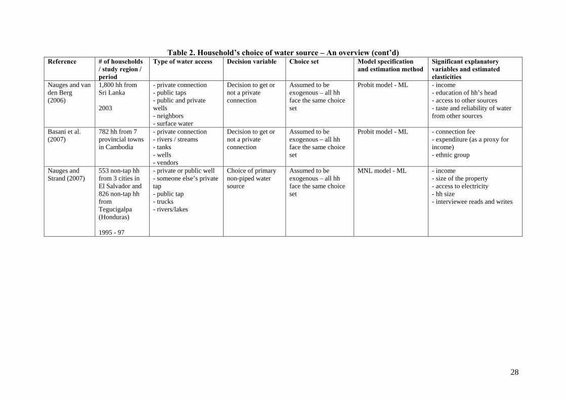
Table 2. Household’s choice of water source – An overview (cont’d) Reference # of households

/ study region / period

Type of water access Decision variable Choice set Model specification and estimation method


Nauges and van den Berg (2006)

1,800 hh from Sri Lanka 2003

- private connection - public taps - public and private wells - neighbors - surface water



Probit model - ML - income - education of hh’s head - access to other sources - taste and reliability of water from other sources

Basani et al. (2007)

782 hh from 7 provincial towns in Cambodia

- private connection - rivers / streams - tanks - wells - vendors



Probit model - ML - connection fee - expenditure (as a proxy for income) - ethnic group

Nauges and Strand (2007)

553 non-tap hh from 3 cities in El Salvador and 826 non-tap hh from Tegucigalpa (Honduras) 1995 - 97

- private or public well - someone else’s private tap - public tap - trucks - rivers/lakes

Choice of primary non-piped water source


MNL model - ML - income - size of the property - access to electricity - hh size - interviewee reads and writes

28

Estimation of Water Demand in Developing … of Water Demand in Developing Countries - An Overview...

Documents

Transcript of Estimation of Water Demand in Developing … of Water Demand in Developing Countries - An Overview...