Aggregate Bank Capital and Credit Dynamics

Nataliya Klimenko∗ Sebastian Pfeil † Jean-Charles Rochet ‡ Gianni De Nicolò §

First draft: December, 2014

This version: March, 2016

Abstract

Central banks need models where the long term impact of macroprudential policies can

be assessed. This paper proposes a model with this feature. In our model commercial banks

�nance their loans with deposits and equity, while facing equity issuance costs. Because of

this �nancial friction, banks build equity bu�ers to absorb negative shocks. Aggregate bank

capital determines the dynamics of credit. Notably, the equilibrium loan rate is a decreasing

function of aggregate capitalization. The competitive equilibrium is constrained ine�cient,

because banks do not internalize the e�ect of their individual lending decisions on the future

loss-absorbing capacity of the banking sector. In particular, we �nd that undercapitalized

banks lend too much. Minimum capital ratios help tame excessive lending, which enhances

stability of the banking system.

Keywords: macro-model with a banking sector, aggregate bank capital, pecuniary externality,

capital requirements

JEL: E21, E32, F44, G21, G28

Acknowledgements: we thank Toni Ahnert, Hengjie Ai, George-Marios Angeletos, Manuel Arellano, Philippe Bac-

chetta, Bruno Biais, Markus Brunnermeier, Catherine Casamatta, Julien Daubanes, Peter DeMarzo, Jean-Paul Décamps,

Sebastian Di Tella, John Geanakoplos, Hans Gersbach, Hendrik Hakenes, Lars Peter Hansen, Zhiguo He, Christian Hellwig,

Florian Ho�mann, Eric Jondeau, Simas Kucinskas, Li (Erica) Xuenan, Michael Magill, Semyon Malamud, Loriano Mancini,

David Martinez-Miera, Erwan Morellec, Alistair Milne, Steven Ongena, Henri Pagès, Bruno Parigi, Greg Phelan, Guillaume

Plantin, Martine Quinzii, Raphael Repullo, Yuliy Sannikov, Enrique Sentana, Amit Seru, Jean Tirole and Stéphane Villeneuve,

and seminar participants at the Banque de France, CEMFI, CICF 2015 conference, Chicago Booth, EPF Lausanne, ETH Zürich,

IMF, MFM Winter 2016 Meeting, Princeton University, Stanford University, Toulouse School of Economics, the University of

Bonn, the University of Nanterre, Yale University.

∗University of Zürich. E-mail: nataliya.klimenko@bf.uzh.ch.†University of Bonn. E-mail: pfeil@uni-bonn.de.‡University of Zürich, SFI and TSE-IDEI. E-mail: jean-charles.rochet@bf.uzh.ch.§International Monetary Fund and CESifo. E-mail: GDeNicolo@imf.org.

1

1 Introduction

In the context of their new macro-prudential responsibilities, central banks have recently been

endowed with powerful regulatory tools. These tools include the setting of capital requirements

for all banks, determining capital add-ons for systemic institutions, and deciding when to activate

counter-cyclical capital bu�ers. The problem is that very little is known about the long term

impact of these regulations on growth and �nancial stability. The DSGE models that central banks

currently have at their disposal have been designed for very di�erent purposes, namely assessing the

short term impact of monetary policy decisions on in�ation and economic activity. Until recently,

DSGE models did not even include banks in their representation of the economy. DSGE models are

very complex and use very special assumptions, because they have been speci�cally calibrated to

reproduce the short term reaction of prices and employment to movements in central banks' policy

rates. It seems therefore clear that complementary models designed to assess the long term impact

of macro-prudential policies on bank credit, GDP growth and �nancial stability are needed. This

paper proposes an example of such a model.

Building on the recent literature on macro models with �nancial frictions, we develop a tractable

dynamic model where aggregate bank capital determines the dynamics of lending. Though highly

stylized, the model is able to generate predictions in line with empirical evidence. Moreover, we

show that our model framework is �exible enough to accommodate the analysis of regulatory policies

by looking at the long-run impact of capital regulation on lending and �nancial stability.

We consider an economy where �rms borrow from banks that are �nanced by deposits, secured

debt and equity. The aggregate supply of bank loans is confronted with the �rms' demand for credit,

which determines the equilibrium loan rate. Aggregate shocks impact the �rms' default probability,

which ultimately translates into pro�ts or losses for banks. Banks can continuously adjust their

volumes of lending to �rms. They also decide when to distribute dividends and when to issue new

equity. Equity issuance is subject to deadweight costs, which constitutes the main �nancial friction

in our economy and creates room for the loss-absorbing role of bank capital.1

In a set-up without the �nancial friction (i.e., no issuance costs for bank equity) and i.i.d.

aggregate shocks, the equilibrium volume of lending and the nominal loan rate would be constant.

Furthermore, dividend payment and equity issuance policies would be trivial in this case: Banks

would immediately distribute all pro�ts as dividends and would issue new shares to o�set losses and

honor obligations to depositors. This implies that, in a frictionless world, there would be no need

to build up capital bu�ers and all loans would be entirely �nanced by debt.

When the �nancial friction is taken into account, banks' dividend and equity issuance strategies

become less trivial. We show that there is a unique competitive equilibrium, where all variables

1Empirical studies report sizable costs of seasoned equity o�erings (see e.g. Lee, Lochhead, Ritter, and Zhao(1996), Hennessy and Whited (2007)). Here we follow the corporate �nance literature (see e.g. Décamps et al. (2011)or Bolton et al. (2011)) and the banking literature (see e.g. De Nicolò et al. (2014)) by assuming that issuing newequity entails a deadweight cost proportional to the size of the issuance.

of interest are deterministic functions of the aggregate book value of bank equity, which follows a

Markov process re�ected at two boundaries. Banks issue new shares at the lower boundary, where

aggregate book equity of the banking system is depleted. When aggregate bank equity reaches its

upper boundary, any further earnings are paid out to shareholders as dividends. Between these

boundaries, the changes in banks' equity are only due to their pro�ts and losses. Banks retain

earnings in order to increase their loss-absorbing equity bu�er that allows them to guarantee the

safety of issued debt claims, while avoiding raising new equity too frequently.2 The target size of

this loss-absorbing bu�er is increasing with the magnitude of the �nancial friction.

We start by exploring the properties of the competitive equilibrium in the �laissez-faire� envi-

ronment, in which banks face no regulation. Even though all agents are risk neutral, our model

generates a positive spread for bank loans. This spread is decreasing in the level of aggregate bank

capital. To get an intuition for this result, note that bank equity is more valuable when it is scarce.

Therefore, the marginal (or market-to-book) value of equity is higher when total bank equity is

lower. Moreover, as pro�ts and losses are positively correlated across banks, each bank anticipates

that aggregate bank equity will be lower (higher) in the states of the world where it makes losses

(pro�ts). Individual losses are thus ampli�ed by a simultaneous increase in the market-to-book

value, whereas individual pro�ts are moderated by a simultaneous decrease in the market-to-book

value. As a result, banks only lend to �rms when the loan rate incorporates an appropriate premium.

To show that the competitive equilibrium is constrained ine�cient, we compare it with the

socially optimal allocation. Our analysis reveals two channels of welfare-reducing pecuniary exter-

nalities. On the one hand, we �nd that competitive banks do not internalize the impact of their

individual lending decisions on i) the banking system's exposure to aggregate shocks and ii) the

pro�t margin on lending. When the banking system is poorly capitalized, banks lend too much as

compared to the socially optimal level, thereby, creating ine�ciently high exposure to aggregate risk.

Furthermore, as excessive lending put downward pressure on banks' pro�t margins, it undermines

the banking system's ability to accumulate loss absorbing capital through retained earnings. On

the other hand, overexposure to aggregate risk in the states with poor capitalization makes banks

e�ectively more risk-averse when the banking system is well capitalized. As a result, well-capitalized

banks lend too little as compared to the social optimum.

As an illustration of the potential of our framework to accommodate the analysis of macropru-

dential policy tools, we use our model to explore the e�ects of minimum capital requirements. A

standard argument against high capital requirements is that they would reduce lending and growth.

By contrast, the proponents of higher capital requirements put emphasis on their positive impact

on �nancial stability. To consider the interplay between the aforementioned e�ects and get some

2The idea that bank equity is needed to guarantee the safety of banks' debt claims is explored in several recentpapers. Stein (2012) shows its implication for the design of monetary policy. Hellwig (2015) develops a static generalequilibrium model where bank equity is necessary to support the provision of safe and liquid investments to consumers.DeAngelo and Stulz (2014) and Gornall and Strebulaev (2015) argue that, due to the banks' ability to diversify risk,the actual size of this equity bu�er may be very small.

2

insights into the long run consequences of capital regulation, we solve the competitive equilibrium

under the regulatory constraint that requires banks to maintain capital ratios above a constant

minimum level.

This analysis yields several results. First, when the minimum capital ratio is not too high, the

regulatory constraint is binding in poorly-capitalized states and is slack in well-capitalized states. In

other words, faced with moderate capital requirements, well-capitalized banks tend to build bu�ers

on top of the required minimum level of capital. By contrast, above some critical level of minimum

capital ratios, the regulatory constraint is always binding, so that banks operate without extra

capital cushions.

Second, a higher capital ratio translates into a higher loan rate and thus reduces lending for

any given level of bank capitalization. Importantly, this e�ect is present even when the regulatory

constraint is slack, because banks anticipate that capital requirements might be binding in the

future and require a higher lending premium for precautionary motives. Thus, provided it is not

too high, a constant capital ratio mitigate ine�ciencies (excessive lending) in poorly capitalized

states, but exacerbates ine�ciencies (insu�cient lending) in well capitalized states. By contrast,

for high minimum capital ratios, lending is ine�ciently low in all states.

Finally, we look at the impact of a constant minimum capital ratio on �nancial stability, by ana-

lyzing the properties of the probability distribution of aggregate capital across states. Surprisingly,

we �nd that imposing mild capital requirements induces the system to spend a lot of time in the

states with low aggregate capitalization. The explanation for this �trap" induced by regulation is

rooted in the interplay between the scale of endogenous volatility in the region where the regulatory

constraint is slack and the region where the regulatory constraint is binding. In fact, even a very

low minimum capital ratio induces a substantial reduction in lending and, thus, in the endogenous

volatility in the constrained region (i.e., in the poorly capitalized states). By contrast, in the un-

constrained region (i.e., in the well capitalized states), the endogenous volatility is almost as high

as in the unregulated set-up. Thus, the system enters the poorly capitalized states almost as often

as in the unregulated set-up, but gets trapped there because of the substantially reduced endoge-

nous volatility. As the minimum capital ratio increases, the di�erences in the endogenous volatility

across states becomes less pronounced. Furthermore, due to higher loan rates, banks bene�t from

higher expected pro�ts, which fosters accumulation of earnings in the banking sector. As a result,

the system enters undercapitalized states less frequently and the "trap" disappears. For very high

levels of capital requirements, the regulated system becomes even more stable than in the social

planner's allocation. However, this �extra� stability comes at the cost of severely reduced lending

and output.

Related literature. Our paper pursues the e�ort of the growing body of the continuous-time

macroeconomic models with �nancial frictions (see e.g. Brunnermeier and Sannikov (2014, 2015),

Di Tella (2015), He and Krishnamurthy (2012, 2013), Phelan (2015)). Seeking for a better un-

3

derstanding of the transmission mechanisms and the consequences of �nancial instability, all these

papers point out to the key role that balance-sheet constraints and net-worth of �nancial interme-

diaries may play in (de)stabilizing the economy in the presence of �nancing frictions and aggregate

shocks. However, the aforementioned works do not explicitly distinguish �nancial intermediaries

from the productive sector (even all of them use "�nancial intermediaries" as a metaphor for the

most productive agents in the economy). We extend this literature by modeling the banking system

explicitly, i.e., by separating the production technology from �nancial intermediation, which enables

us to explore the impact of the bank lending channel on �nancial stability.

A common feature of the above-mentioned papers is the existence of �re-sale externalities in the

spirit of Kiyotaki and Moore (1997) and Lorenzoni (2008) that arise when forced asset sales depress

prices, triggering amplifying feedback e�ects. In our model, welfare-reducing pecuniary externalities

in the credit market emerge in the absence of costly �re-sales, stemming from the di�erence between

the social and private implied risk aversion with respect to the variations of aggregate bank capital.

The main channel of ine�ciencies imposed by individual banks' lending decisions is that each bank

fails to internalize the impact of its lending choice on the banking system's exposure to aggregate

risk, which increases endogenous volatility. An additional channel of ine�ciencies is that individual

banks do not internalize the impact of their lending decisions on the size of the expected pro�t

margins, which is similar to the e�ect described in Malherbe (2015). However, whereas in Malherbe

(2015), this �margin channel� a�ects social welfare via the size of the bankruptcy costs for all

banks in the economy, in our framework it has the dynamic welfare implications. Namely, expected

pro�t margins a�ect the ability of banks to accumulate loss-absorbing capital and thus their future

capacity to lend.

From a technical perspective, our paper is related to the corporate liquidity management litera-

ture (see e.g. Jeanblanc and Shiryaev (1996), Milne and Robertson (1996), Décamps et al. (2011),

Bolton et al. (2011, 2013), Hugonnier et Morellec (2015) among others) that places emphasis on the

loss-absorbing role of corporate liquid reserves in the presence of �nancial frictions. In our model,

the role of book equity is very similar to the role of liquidity bu�ers in those models. However, we

di�erentiate from this literature by allowing for the feedback loop between the individual decisions

and the dynamics of individual book equity via the general equilibrium mechanism that determines

the loan rate and thus a�ects the expected earnings of banks. As a result, the individual bank's

policies are driven by aggregate rather than individual book equity.

Our paper is also linked to the vast literature exploring the welfare e�ects of bank capital

regulation. Most of the literature dealing with this issue is focused on the trade-o� between the

welfare gains from the mitigation of risk-taking incentives on the one hand and welfare losses caused

by lower liquidity provision (e.g., Begenau (2015), Van den Heuvel (2008)), lower lending and output

(e.g., Nguyên (2014), Martinez-Miera and Suarez (2014)) on the other hand.3 In contrast to the

3The only exception is the work by De Nicolò et al. (2014) that conducts the analysis of bank risk choices undercapital and liquidity regulation in a fully dynamic model, where capital plays the role of a shock absorber, and

4

above-mentioned studies, the focus of our model is entirely shifted from the incentive e�ect of bank

capital towards its role of a loss absorbing bu�er - the concept that is often put forward by bank

regulators. Moreover, the main contribution of our paper is qualitative: we seek to identify the long

run e�ects of capital regulation rather than to provide a quantitative guidance on the optimal level

of a minimum capital ratio.

More broadly, this paper relates to the literature on credit cycles that has brought forward a

number of alternative explanations for their occurrence. Fisher (1933) identi�ed the famous debt

de�ation mechanism, that has been further formalized by Bernanke et al. (1996) and Kiyotaki and

Moore (1997). It attributes the origin of credit cycles to the �uctuations of the prices of collateral.

Several studies also emphasize the role of �nancial intermediaries, by pointing out the fact that credit

expansion is often accompanied by a loosening of lending standards and "systemic" risk-taking,

whereas materialization of risk accumulated on the balance sheets of �nancial intermediaries leads to

the contraction of credit (see e.g. Aikman et al. (2014), Dell'Ariccia and Marquez (2006), Jimenez

and Saurina (2006)). In our model, quasi-cyclical lending patterns emerge due to the re�ection

property of aggregate bank capital that follows from the optimality of �barrier� recapitalization and

dividend strategies.

The rest of the paper is organized as follows. Section 2 presents the model. In Section 3 we

characterize the competitive equilibrium. In Section 4, we discuss the long run behavior of the

economy. Section 5 studies the sources of ine�ciencies and compares the competitive equilibrium

with the social planner's allocation. In Section 6 we introduce capital regulation, analyzing its

implications for bank policies and the lending-stability trade-o�. Section 7 concludes. All proofs

and computational details are gathered in the Appendix. The empirical analysis supporting the key

model predictions and additional materials can be found in the Online Appendix.

2 Model

The economy is populated by households, who own and manage banks, and entrepreneurs, who

own and manage �rms (see Figure 1). All agents are risk-neutral and have the same discount

rate ρ. An entity labelled �central bank� serves to equilibrate the interbank lending market, by

o�ering (perfectly elastic) reserve and re�nancing facilities. There is one physical good, taken as a

numeraire, which can be consumed or invested.

2.1 Economy

Firms. We consider an economy where the volume of bank lending determines the volume of

productive investment. Entrepreneurs can consume only positive amounts and cannot save. At

dividends, retained earnings and equity issuance are modeled under a �nancial friction captured by a constraint oncollateralized debt.

5

Figure 1: The structure of the economy

tKLoans

tE

Liabilities

Equity

Banking sector

Loans

RepaymentsHouseholds

Profits

Interests on

deposits

Dividends

Firms

Reserves

Entrepreneurs

any time t each �rm is endowed with a project that requires an investment of 1 unit of good and

produces xh units of good at time t+h. The productivity parameter x is distributed according to a

continuous distribution with density function f(x) de�ned on a bounded support [0, R]. To �nance

the investment project, a �rm can take up a bank loan, for which it has to repay 1 + Rth (to be

determined in equilibrium) at time t+ h.4

For the sake of exposition, we assume that a �rm can always repay the interest, while the

productive capital (principal) is destroyed with probability pt(h).5 Since the return on investment

for a �rm with productivity x is always equal to x− Rt, a �rm asks for a bank loan and invests if

and only if x ≥ Rt. The total demand for bank loans at time t is, thus, given by

L(Rt) ≡∫ R

Rt

f(x)dx. (1)

Firms are subject to aggregate shocks that a�ect the probability of productive capital being

destroyed. More speci�cally, �rms' default probability pt(h) is higher under a negative shock and

is lower under a positive shock, i.e.,

pt(h) =

ph− σ0

√h, with probability 1/2 (positive shock)

ph+ σ0

√h, with probability 1/2 (negative shock)

, (2)

4Firms in our model should be thought of as small and medium-sized enterprises (SMEs), which typically rely onbank �nancing. As is well known, the importance of bank �nancing varies across countries. For example, accordingto the TheCityUK research report (October 2013), in EU area, bank loans account for 81% of the long term debt inthe real sector, whereas in the U.S. the same ratio amounts to 19%.

5The assumption that R is always repaid is, of course, completely inconsequential in the continuous-time limitthat we consider throughout the main analysis.

6

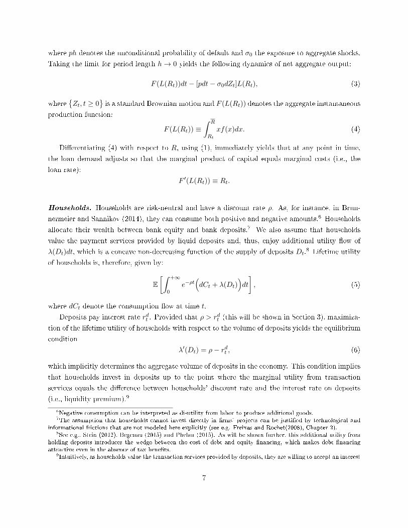
where ph denotes the unconditional probability of default and σ0 the exposure to aggregate shocks.

Taking the limit for period length h→ 0 yields the following dynamics of net aggregate output:

F (L(Rt))dt− [pdt− σ0dZt]L(Rt), (3)

where{Zt, t ≥ 0

}is a standard Brownian motion and F (L(Rt)) denotes the aggregate instantaneous

production function:

F (L(Rt)) ≡∫ R

Rt

xf(x)dx. (4)

Di�erentiating (4) with respect to R, using (1), immediately yields that at any point in time,

the loan demand adjusts so that the marginal product of capital equals marginal costs (i.e., the

loan rate):

F ′(L(Rt)) ≡ Rt.

Households. Households are risk-neutral and have a discount rate ρ. As, for instance, in Brun-

nermeier and Sannikov (2014), they can consume both positive and negative amounts.6 Households

allocate their wealth between bank equity and bank deposits.7 We also assume that households

value the payment services provided by liquid deposits and, thus, enjoy additional utility �ow of

λ(Dt)dt, which is a concave non-decreasing function of the supply of deposits Dt.8 Lifetime utility

of households is, therefore, given by:

E[∫ +∞

0e−ρt

(dCt + λ(Dt)

)dt

], (5)

where dCt denote the consumption �ow at time t.

Deposits pay interest rate rdt . Provided that ρ > rdt (this will be shown in Section 3), maximiza-

tion of the lifetime utility of households with respect to the volume of deposits yields the equilibrium

condition

λ′(Dt) = ρ− rdt , (6)

which implicitly determines the aggregate volume of deposits in the economy. This condition implies

that households invest in deposits up to the point where the marginal utility from transaction

services equals the di�erence between households' discount rate and the interest rate on deposits

(i.e., liquidity premium).9

6Negative consumption can be interpreted as disutility from labor to produce additional goods.7The assumption that households cannot invest directly in �rms' projects can be justi�ed by technological and

informational frictions that are not modeled here explicitly (see e.g. Freixas and Rochet(2008), Chapter 2).8See e.g., Stein (2012), Begenau (2015) and Phelan (2015). As will be shown further, this additional utility from

holding deposits introduces the wedge between the cost of debt and equity �nancing, which makes debt �nancingattractive even in the absence of tax bene�ts.

9Intuitively, as households value the transaction services provided by deposits, they are willing to accept an interest

7

Banks. Each bank has access to central bank reserves and re�nancing facilities (or, equivalently, to

interbank lending) at the exogenously given, constant central bank (or, equivalently, money market)

rate r < ρ. At time t, a given bank with et ≥ 0 units of equity chooses the amount of deposits,

dt ≥ 0, and the volume of lending to �rms, kt ≥ 0. Its net position of reserves in the central

bank (or/and lending on the interbank lending market) is determined by the following accounting

identity:

mt = et + dt − kt. (7)

A bank also chooses the amount of dividends to be distributed to existing shareholders dδt ≥ 0,

and the amount of new equity to be raised, dit ≥ 0. Issuing equity entails a proportional (dead-

weight) cost γ, which constitutes the main �nancial friction in our economy. Note that in the

presence of this �nancial friction and aggregate shocks, bank equity will serve the purpose to bu�er

losses on loans.

Banks supply loans in a perfectly competitive market and, thus, take the loan rate Rt as given.

When a bank grants a loan to �rms, it bears the risk that the principal will be destroyed, implying

that the instantaneous cash �ow generated by 1 unit of loans is given by (1 + Rt − p)dt − σ0dZt.

Thus, book equity of a given bank evolves according to:

et+dt = kt[(1 +Rt − p)dt− σ0dZt]− dδt + dit + (1 + r)mtdt− (1 + rdt )dtdt,

which, given accounting identity (7), can be rewritten as follows:

det = retdt+ kt[(Rt − p− r)dt− σ0dZt]− dδt + dit + dt(r − rdt )dt. (8)

Similarly, aggregate bank equity Et, evolves according to:

dEt = rEtdt+Kt[(Rt − p− r)dt− σ0dZt]− d∆t + dIt +Dt(r − rdt )dt, (9)

where Kt, d∆t, dIt, and Dt denote, respectively, the aggregate volumes of lending, dividends, equity

issuance, and deposits at time t.

Each bank is run in the interest of its shareholders, implying that lending, deposit, dividend,

and recapitalization policies are chosen so as to maximize shareholder value

v(e, E) = maxkt,dt,dδt,dit

E[∫ τ

0e−ρt

(dδt − (1 + γ)dit

)|e0 = e, E0 = E

], (10)

where individual and aggregate equity follow (8) and (9) respectively, and τ := inf{t : et < 0}denotes the �rst time when the book value of bank equity becomes negative, which triggers the

bank's default. If it is optimal to inject new equity instead of defaulting, τ ≡ ∞. We assume

rate below the discount rate.

8

throughout that this is, in fact, the case and provide the appropriate condition in the proof of

Proposition 2.

2.2 One-period example

Before turning to the analysis of the competitive equilibrium of the dynamic model, it is instruc-

tive to brie�y consider a one-period problem to illustrate the basic frictions in our framework. In

t = 0, each bank has an initial endowment of equity e0, deposit d, issues new equity i, distributes

dividends δ, and grants loans k to �rms. Returns are realized, claims are repaid, and consumption

takes place at t = 1. For a period length normalized to one, �rms' default probability is p ≡ p∓σ0.

The accounting identity (7) then becomes

m = e0 − δ + i+ d− k, (11)

and bank pro�ts at date t = 1 can be written as

πB = (1 + r)e+ k(R− p− r) + d(r − rd), (12)

where e ≡ e0 − δ + i denotes an individual bank's equity after recapitalization and dividend distri-

bution. Note that for the deposit market to clear, the deposit rate must coincide with the central

bank rate, rd ≡ r, implying that the last term in (12) vanishes. Conditional on the realization of

the aggregate shock, a given bank's equity in t = 1 is then given by

e+ ≡ (1 + r)e+ k[R− r − (p− σ0)

],

e− ≡ (1 + r)e+ k[R− r − (p+ σ0)

].

To make the non-negativity constraint for equity meaningful in the one-period problem, we

assume that interbank lending is fully collateralized.10 Thus, bank capital must be su�ciently high

to cover the worst possible loss:

e− ≥ 0. (13)

Imposing this collateral constraint generates a role for bank capital as a loss absorbing bu�er in this

static set-up. However, this is merely a short-cut formulation for the endogenous bene�ts of capital

bu�ers that arise in the dynamic setting.

A competitive equilibrium is characterized by a loan rateR which, by market clearing, determines

the aggregate volume of lending K ≡ L(R). Each bank takes the loan rate R as given and chooses

10This condition easily extends to the case when depositors accept some probability of default (Value-at-Riskconstraint similar to Adrian and Shin (2010)). An equivalent interpretation is that banks �nance themselves byrepos, and the lender applies a hair cut equal to the maximum possible value of the asset (the loan portfolio) that isused as collateral.

9

dividend policy δ ≥ 0, recapitalization policy i ≥ 0 and the volume of lending k ≥ 0 so as to

maximize shareholder value,

v = maxδ,i,k

{δ − (1 + γ)i+

(12

)e+ +

(12 + θ

)e−

1 + ρ

},

where θ denotes the Lagrange multiplier associated with the constraint (13).11 Note that this

problem is separable, i.e.,

v = e0u+ maxδ≥0

δ[1− u

]+ max

i≥0i[u− (1 + γ)

]+ max

k≥0k[(R− p− r)(1 + θ)− θσ0

1 + ρ

], (14)

where

u ≡ (1 + r)(1 + θ)

1 + ρ. (15)

Optimizing with respect to the bank's policies yields the following conditions:

1− u ≤ 0 (= if δ > 0), (16)

u− (1 + γ) ≤ 0 (= if i > 0), (17)

− R− r − pR− r − (p+ σ0)

≥ θ (= if k > 0). (18)

Condition (16) shows that θ > 0, which implies that constraint (13) is always binding at both

the individual and aggregate level. This determines the loan rate as a function of aggregate bank

capitalization, i.e. R ≡ R(E). More speci�cally, rewriting the binding constraint (13) for aggregate

equity yields

(1 + r)E + L(R(E))[R(E)− r − (p+ σ0)

]= 0. (19)

Two implications immediately follow from this expression: i) the equilibrium loan rate R ≡ R(E)

is a decreasing function of aggregate capital and ii) the aggregate volume of lending is strictly

positive. Hence, equation (18) must hold with equality and pins down the shadow cost function

θ ≡ θ(E). Substituting (15) through (18) into (14), we �nd that the shareholder value function of

each bank is proportional to its book equity and explicitly given by

v = e0u(E) = e0

(1 + r

1 + ρ

)(−σ0

R(E)− r − (p+ σ0)

), (20)

where u ≡ u(E) is the market-to-book value of equity. Note that u(E) is a decreasing function of

E, implying that bank capital becomes more valuable when it is getting scarce.

Conditions (16) and (17) show that the optimal dividend and recapitalization policies also depend

on aggregate capital via the market-to-book value of bank equity. Let Emax denote the unique level

11In this one-period model, shareholders receive terminal dividends at the end of the period.

10

of aggregate equity such that (16) holds with equality, and Emin the one such that (17) holds with

equality. Then, if E < Emin, shareholders will recapitalize banks by raising in aggregate Emin−E.Similarly, if E > Emax, aggregate dividends E −Emax are distributed to shareholders. As a result,

the market-to-book ratio of the banking sector always belongs to the range [1, 1 + γ]. The following

proposition summarizes our results for this static set-up:

Proposition 1 The one-period model has a unique competitive equilibrium, where

a) The loan rate R ≡ R(E) is a decreasing function of aggregate capital and it is implicitly given

by the binding non-negativity constraint for aggregate capital (19).

b) All banks have the same market-to-book ratio of equity given by (20), which is a decreasing

function of aggregate capital.

c) Banks pay dividends when E ≥ Emax ≡ u−1(1) and recapitalize when E ≤ Emin ≡ u−1(1 + γ).

Despite the simplistic approach, modelling the need for capital bu�ers in such a reduced form

allows us to illustrate several important features that prevail in the continuous-time equilibrium.

First, only the level of aggregate bank capital E matters for banks' policies, whereas the individual

banks' sizes do not play any role. Second, banks' recapitalization and dividend policies are of the

"barrier type" and are driven by the market-to-book value of equity which, in turn, is strictly

decreasing in aggregate bank capital and remains in the interval [1, 1 + γ]. Finally, the loan rate is

decreasing in aggregate bank capital.

3 Competitive Equilibrium

3.1 Solving for the equilibrium

In this section we solve for a Markovian competitive equilibrium, where all aggregate variables

are deterministic functions of the single state variable, namely, aggregate bank equity, Et. In a

competitive equilibrium, i) loan and deposit markets must clear; ii) the dynamic of individual and

aggregate bank capital is given by (8) and (9), respectively; iii)banks maximize (10).

Consider �rst the optimal decision problem of an individual bank that chooses lending kt ≥ 0,

deposit dt ≥ 0, dividend dδt ≥ 0 and recapitalization dit ≥ 0, so as to maximize shareholder value.

Making use of the homotheticity property of the equity market value de�ned in (10), we de�ne the

market-to-book value of bank capital,

u(E) ≡ v(e, E)

e,

which can also be interpreted as the marginal value of an individual bank's book equity, e. Note

that this allows to work with aggregate bank capital, E, as the single state variable and, thus, to

11

focus on the capitalization of the banking sector as a whole, instead of the capitalization of each

individual bank. By standard dynamic programming arguments, the market-to-book value of a

given bank in the economy satis�es the following Bellman equation:

(ρ− r)u(E) = maxdδ≥0

{dδe

[1− u(E)]}−max

di≥0

{die

[1 + γ − u(E)]}

+ maxd≥0

{de

(r − rdt )u(E)}

+ maxk≥0

{ke

[(R(E)− p− r)u(E) + σ2

0K(E)u′(E)]}

+(rE +K(E)[R(E)− p− r]

)u′(E) +

σ20K

2(E)

2u′′(E).

(21)

Maximization with respect to the volume of deposits shows that the deposit market clears only

if the deposit rate coincides with the central bank rate, i.e. rdt ≡ r. This implies that an individual

bank is indi�erent with respect to the volume of deposits. Using (6), it is easy to see that, on

the aggregate level, the volume of deposits is constant and can be pinned down from equation

λ′(D) = ρ − r. Moreover, with rdt ≡ r, the last terms in the equations (8) and (9) describing the

dynamics of individual and aggregate equity vanish.

Since banks are competitive, each bank takes the loan rate R(E) as given. For the loan market to

clear, the aggregate supply of loans has to equal �rms' demand for loans in (1) under the prevailing

loan rate, i.e. K(E) = L(R(E)).12 Maximizing (21) with respect to the loan supply of each

individual bank shows that for lending to be interior, the risk-adjusted loan spread must equal

banks' risk-premium:

R(E)− p− r = −u′(E)

u(E)σ2

0L(R(E)). (22)

The risk-premium required by any given bank is driven by its implied risk aversion with respect

to variation in aggregate capital, −u′(E)/u(E), multiplied by the endogenous volatility of aggregate

capital, σ20L(R(E)). Since an additional unit of loss absorbing capital in the banking sector is more

valuable when it is scarce, the market-to-book ratio u(E) is (weakly) decreasing in aggregate capital

(this is shown formally in the proof of Proposition 2). Intuitively, risk-neutral banks become risk-

averse with respect to variations in aggregate capital and therefore require a positive risk premium

due to the following ampli�cation e�ect: Upon the realization of a negative aggregate shock, the

capitalization of the banking system deteriorates, which drives up the market-to-book value u(E)

and, thus, aggravates the impact of the negative shock on each individual bank's shareholder value

(recall that v(e, E) ≡ eu(E)). Conversely, upon the realization of a positive aggregate shock, the

banking system will be better capitalized, which reduces the market to book ratio u(E) and, thus,

reduces the impact of the positive shock on shareholder value of any individual bank.

Next, optimization with respect to dδ and di shows that the optimal dividend and recapitaliza-

12This speci�cation is analogous to an economy with constant returns to scale, in which the equilibrium price ofany output is only determined by technology (constant marginal cost), whereas the volume of activity is determinedby the demand side.

12

tion policies are of the "barrier" type. That is, each individual bank distributes dividends (dδ > 0)

when the level of aggregate bank capital exceeds a critical level Emax, that satis�es

u(Emax) = 1, (23)

i.e., the marginal value of equity capital equals the shareholders' marginal value of consumption.

Aggregate dividend payments therefore consist of all pro�ts in excess of Emax, which induces the

aggregate capital process to be re�ected at that point.

Moreover, the absence of arbitrage opportunities on the bank equity market implies that, at

Emax, the marginal change in the value of total bank equity claim must equal the marginal value

of consumtion, i.e., [Eu(E)]′ = 1. Together with (23), this condition implies that u′(Emax) = 0. As

a result, at the dividend payout boundary, the required risk-premium in (22) vanishes, i.e.,

R(Emax) = p+ r. (24)

That is, as banks make zero expected pro�ts on the marginal loan, all capital in excess of Emax is

distributed to shareholders rather than invested in the corporate loan market.

Similarly, new equity is issued (di > 0) only when aggregate capital reaches a critical threshold

Emin at which the marginal value of equity equals the total marginal cost of equity issuance, i.e.,

u(Emin) = 1 + γ. (25)

At that point, all banks issue new equity to o�set further losses on their loan portfolios and, thus,

to prevent aggregate equity from falling below Emin. Since the market to book ratio u(E) is (weakly)

decreasing in aggregate capital, banks recapitalize only if all capital is completely exhausted and,

thus, the non-negativity constraint binds on the individual and on the aggregate level.13 Taken

together, aggregate bank equity �uctuates between the re�ecting barriers,

Emin = 0,

where all banks recapitalize, and Emax, where all banks pay dividends. In the interior region

(0, Emax), banks retain all pro�ts to build up capital bu�ers and use these bu�ers to o�set losses.

13In the Online Appendix, we show that, in the discrete-time dynamic version of the model, banks are recapitalizedat a strictly positive level of E. The reason is that, in the discrete-time dynamic set-up, the non-negativity con-straint for capital is binding for low levels of equity both at the individual and at the aggregate level. Acceleratingrecapitalizations allows shareholders to reduce the �shadow costs� of the binding non-negativity constraint. However,when the length of the time period goes to zero, the region on which the non-negativity constraint is binding shrinks(and collapses to a single point, 0, in the continuous-time limit). It is important to stress, however, that the propertyEmin = 0 is not a general feature of the continuous-time set-up. In the Online Appendix we show that the recapital-ization barrier may depend on the state of the business cycle, similar in spirit to the �market timing� result of Boltonet al. (2013).

13

For E ∈ (0, Emax), the market-to-book value u(E) satis�es

(ρ− r)u(E) =[rE + L(R(E))

(R(E)− p− r

)]u′(E) +

σ20L(R(E))2

2u′′(E). (26)

The following proposition characterizes the competitive equilibrium.

Proposition 2 There exists a unique Markovian equilibrium, in which aggregate bank capital evolves

according to:

dEt = rEtdt+ L(R(Et))[(R(Et)− p− r)dt− σ0dZt

]. (27)

The equilibrium loan rate R(E) and market-to-book value u(E) satisfy (22) through (26). Banks

distribute dividends when E reaches the threshold Emax and recapitalize when E reaches 0.

To illustrate the properties of the obtained equilibrium, we use expression (22) to eliminate the

market-to-book value (and its derivatives) in the second order di�erential equation (26). This yields

a relatively simple �rst order di�erential equation in R(E),

R′(E) ≡ H(E,R(E)) := −(

1

σ20

)2(ρ− r)σ2

0 +[R(E)− p− r

]2+ 2rE

[R(E)− p− r

]L(R(E))−1

L(R(E))− L′(R(E))[R(E)− p− r

] .

(28)

From (28) it is immediate, that the loan rate R(E) is strictly decreasing in E. That is, as the

banking system becomes better capitalized, banks' implied risk-aversion −u′(E)/u(E) decreases

which, despite an increase in the endogenous volatility of aggregate capital σ20L(R(E)), results in a

lower risk-premium in expression (22).14

Moreover, solving equation (22) subject to boundary condition (23), yields the quasi-explicit

expression for the market-to-book value:

u(E) = exp(∫ Emax

E

R(s)− p− rσ2

0L(R(s))ds), (29)

where R(E) satis�es (28) with the boundary condition R(Emax) = p+ r.

The free boundary Emax is then pinned down by boundary condition (25), which transforms to:∫ Emax

0

R(s)− p− rσ2

0L(R(s))ds = ln(1 + γ). (30)

The fact thatR(E) is a decreasing function of E that satis�es the boundary conditionR(Emax) =

p + r implies that the loan rate increases with Emax for any level of E. It is then easy to see that

the left-hand side of Expression (30) is increasing in Emax. This immediately leads to the following

result:14Since aggregate output in our economy is completely determined by the volume of bank lending, this gives rise

to pro-cyclical lending patterns in line with empirical evidence reported, for instance, by Becker and Ivashina (2014).

14

Corollary 1 The target level of aggregate bank capital, Emax, is increasing with the magnitude of

�nancial friction γ.

Intuitively, stronger �nancial frictions make bank shareholders e�ectively more risk averse, which

induces them to postpone dividend payments to build larger capital bu�ers. Simultaneously, a higher

e�ective risk aversion implies higher loan rates. Thus, our model suggests that lending and, thereby,

output should exhibit more dispersion in the economies with stronger �nancial frictions.

3.2 Testable implications

Overall, the analysis conducted above delivers two key testable predictions: the equilibrium

loan rate and the banks' market-to-book ratio of equity should be decreasing functions of aggregate

bank capital. To examine whether these predictions are rejected by the data or not, in Appendix

III we conduct statistical tests on a data set covering a large panel of publicly traded banks in 43

advanced and emerging market economies for the period 1992-2012. We �nd that our predictions

�t the data extremely well. Table 4 in Appendix III shows the results of simple regressions of loan

rates and market-to-book ratios of banks equity in four sub-panels: U.S. banks, Japanese banks,

Advanced countries' (excluding U.S. and Japan) banks and Emerging countries' banks. In all cases,

the coe�cients of Total Bank Equity are negative with p-values indistinguishable from zero, which

indicates that two key predictions of our model are consistent with the data.

3.3 Parameter choice

For the rest of the paper, we adopt the particular speci�cation of the demand for loans:

L(R) =( R−RR− p− r

)β, (31)

where β ≥ 0 is the elasticity parameter. In the above speci�cation the volume of credit is normalized

by its frictionless level.

Table 1: Parameter values

Parameter Symbol Feasible values

Discount rate ρ [0.02, 0.05]Money market rate r [0, ρ)Unconditional default probability of �rms p [0.02, 0.04]

Maximum feasible loan rate R [0.2, 0.3]Elasticity parameter β [0, 1.2]Risk exposure σ0 [0.05, 0.1]Financial friction γ [0.01, 0.5]

15

Table 1 summarizes the set of parameter values used in our further numerical analysis. The

admissible range for the discount rate ρ generates the discount factors in the range [0.98, 0.95], which

is consistent with empirical evidence. The range of the maximum feasible loan rate is consistent

with the maximum rates of returns on bank assets observed in our data sample. The range for the

unconditional probabilities of default in the real sector re�ects the average default probabilities in

the industrial sector estimated by Condrad et al. (2013). Elasticity parameter β is restricted to

ensure that the absolute value of the semi-elasticity of the loan demand (i.e., |L′(R)/L(R)| = β

R−R) implied by our model does not exceed 10 percentage points. The range of values of the exposure

to exogenous shocks, σ0, is set so as to generate non-negligible variations in lending. Finally, the

range of admissible values for the �nancial friction is chosen based on the market-to-book values

observed in our data sample. For example, for U.S. sub-sample, the average market-to-book value

is about 1.40 which, according to our model, implies that γ > 0.4. It should be mentioned, however,

that the values of the �nancial friction implied by the data are much higher than the typical values

of the �otation costs of equity issuance used in the recent quantitative models of banking (e.g. 0.06

in De Nicolò et al. (2014)) or documented by the corporate �nance literature (e.g., 0.05 − 0.1 in

Hennessy and Whited (2007)), which suggests that γ might admit a broader interpretation.

4 The long-run behavior of the economy

In this section we show that the endogenous risk is the main driver of the long run behavior of the

economy, so that the "deterministic" steady state approach employed by the traditional marcoeco-

nomic models to analyse the long run macrodynamics would lead to substantial misestimations.

4.1 Loan rate dynamics

To illustrate the long run behavior of our economy we focus on the dynamics of the loan rate

Rt.15 For the special case in which the central bank rate r is set to zero, the dynamics of the

loan rate can be obtained in closed form. Let Rt = R(Et) be some twice continuously di�erentiable

function of aggregate capital. Applying Itô's lemma to R(Et), while using the equilibrium dynamics

of Et ∈ (0, Emax) given in (27), yields:

dRt = L(R(Et))(

(R(Et)− p)R′(Et) +σ2

0L(R(Et))

2R′′(Et)

)︸ ︷︷ ︸

µ(Rt)

dt− σ0L(R(Et))R′(Et)︸ ︷︷ ︸

σ(Rt)

dZt. (32)

Recall that the loan rate satis�es the �rst-order di�erential equation (28), which allows us to

eliminate its derivatives from expression (32). After some algebra, one can thus obtain the drift and

15One could equivalently look at the dynamics of the state variable Et. However, in the simple set-up with noregulation, working with Rt instead of Et enables us to analytically characterize the system's behavior, because thedrift and volatility of Rt are closed-form expressions.

16

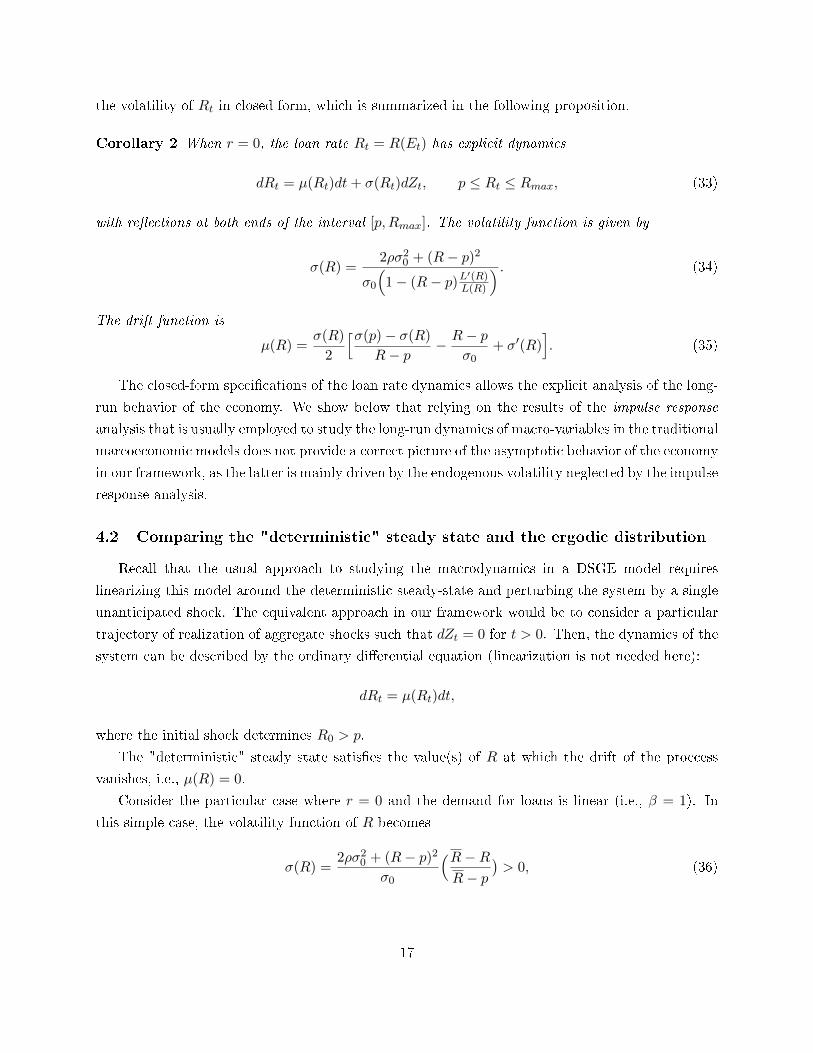
the volatility of Rt in closed form, which is summarized in the following proposition.

Corollary 2 When r = 0, the loan rate Rt = R(Et) has explicit dynamics

dRt = µ(Rt)dt+ σ(Rt)dZt, p ≤ Rt ≤ Rmax, (33)

with re�ections at both ends of the interval [p,Rmax]. The volatility function is given by

σ(R) =2ρσ2

0 + (R− p)2

σ0

(1− (R− p)L

′(R)L(R)

) . (34)

The drift function is

µ(R) =σ(R)

2

[σ(p)− σ(R)

R− p− R− p

σ0+ σ′(R)

]. (35)

The closed-form speci�cations of the loan rate dynamics allows the explicit analysis of the long-

run behavior of the economy. We show below that relying on the results of the impulse response

analysis that is usually employed to study the long-run dynamics of macro-variables in the traditional

marcoeconomic models does not provide a correct picture of the asymptotic behavior of the economy

in our framework, as the latter is mainly driven by the endogenous volatility neglected by the impulse

response analysis.

4.2 Comparing the "deterministic" steady state and the ergodic distribution

Recall that the usual approach to studying the macrodynamics in a DSGE model requires

linearizing this model around the deterministic steady-state and perturbing the system by a single

unanticipated shock. The equivalent approach in our framework would be to consider a particular

trajectory of realization of aggregate shocks such that dZt = 0 for t > 0. Then, the dynamics of the

system can be described by the ordinary di�erential equation (linearization is not needed here):

dRt = µ(Rt)dt,

where the initial shock determines R0 > p.

The "deterministic" steady state satis�es the value(s) of R at which the drift of the proccess

vanishes, i.e., µ(R) = 0.

Consider the particular case where r = 0 and the demand for loans is linear (i.e., β = 1). In

this simple case, the volatility function of R becomes

σ(R) =2ρσ2

0 + (R− p)2

σ0

(R−RR− p

)> 0, (36)

17

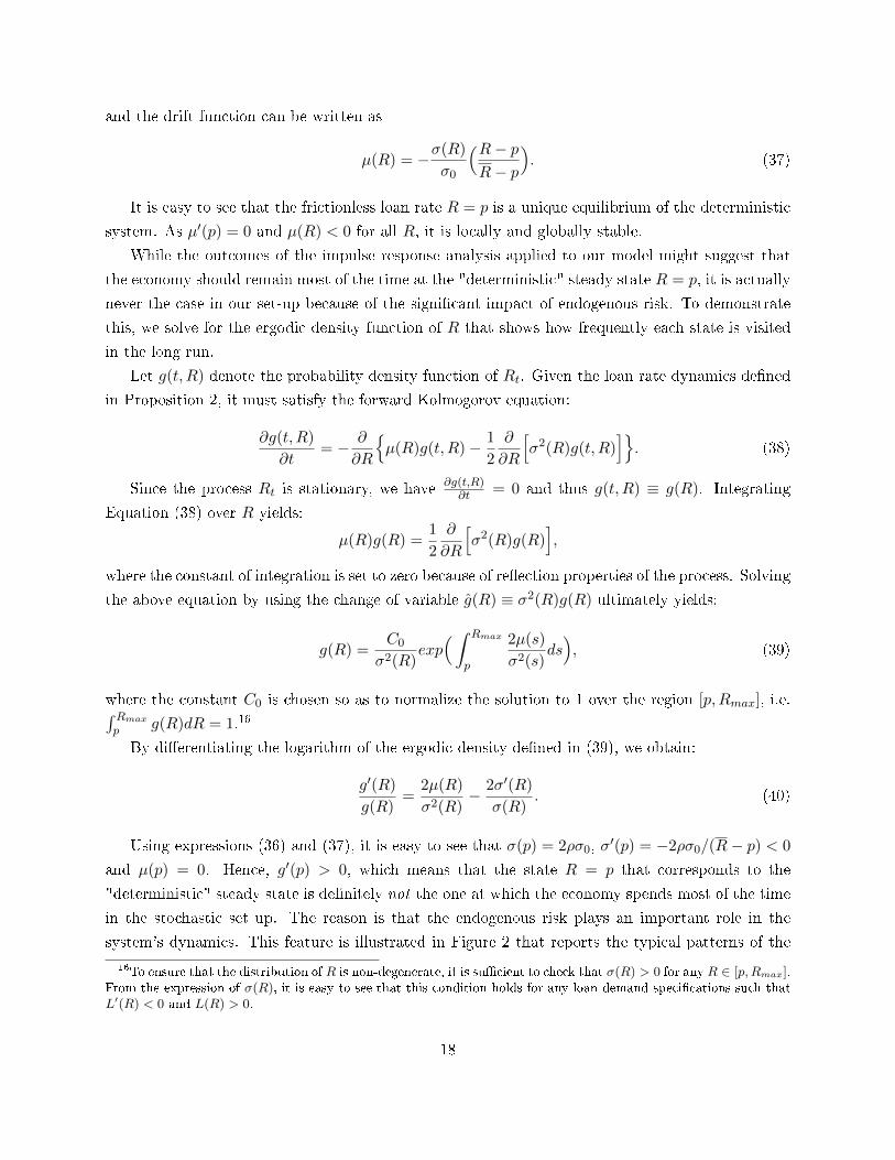
and the drift function can be written as

µ(R) = −σ(R)

σ0

(R− pR− p

). (37)

It is easy to see that the frictionless loan rate R = p is a unique equilibrium of the deterministic

system. As µ′(p) = 0 and µ(R) < 0 for all R, it is locally and globally stable.

While the outcomes of the impulse response analysis applied to our model might suggest that

the economy should remain most of the time at the "deterministic" steady state R = p, it is actually

never the case in our set-up because of the signi�cant impact of endogenous risk. To demonstrate

this, we solve for the ergodic density function of R that shows how frequently each state is visited

in the long run.

Let g(t, R) denote the probability density function of Rt. Given the loan rate dynamics de�ned

in Proposition 2, it must satisfy the forward Kolmogorov equation:

∂g(t, R)

∂t= − ∂

∂R

{µ(R)g(t, R)− 1

2

∂

∂R

[σ2(R)g(t, R)

]}. (38)

Since the process Rt is stationary, we have ∂g(t,R)∂t = 0 and thus g(t, R) ≡ g(R). Integrating

Equation (38) over R yields:

µ(R)g(R) =1

2

∂

∂R

[σ2(R)g(R)

],

where the constant of integration is set to zero because of re�ection properties of the process. Solving

the above equation by using the change of variable g(R) ≡ σ2(R)g(R) ultimately yields:

g(R) =C0

σ2(R)exp(∫ Rmax

p

2µ(s)

σ2(s)ds), (39)

where the constant C0 is chosen so as to normalize the solution to 1 over the region [p,Rmax], i.e.∫ Rmaxp g(R)dR = 1.16

By di�erentiating the logarithm of the ergodic density de�ned in (39), we obtain:

g′(R)

g(R)=

2µ(R)

σ2(R)− 2σ′(R)

σ(R). (40)

Using expressions (36) and (37), it is easy to see that σ(p) = 2ρσ0, σ′(p) = −2ρσ0/(R− p) < 0

and µ(p) = 0. Hence, g′(p) > 0, which means that the state R = p that corresponds to the

"deterministic" steady state is de�nitely not the one at which the economy spends most of the time

in the stochastic set up. The reason is that the endogenous risk plays an important role in the

system's dynamics. This feature is illustrated in Figure 2 that reports the typical patterns of the

16To ensure that the distribution of R is non-degenerate, it is su�cient to check that σ(R) > 0 for any R ∈ [p,Rmax].From the expression of σ(R), it is easy to see that this condition holds for any loan demand speci�cations such thatL′(R) < 0 and L(R) > 0.

18

endogenous volatility σ(R) (the left-hand side panel) and the ergodic density g(R) (the right-hand

side panel) for the speci�cation of the loan demand stated in (31). It shows that the extrema of the

ergodic density mirror those of the volatility function, i.e., the economy spends most of the time in

the states with the lowest loan rate volatility.17

Figure 2: Volatility and ergodic density of R

0.020 0.025 0.030 0.035 0.040 0.045 0.050R

0.005

0.010

0.015

σ(R)

0.020 0.025 0.030 0.035 0.040 0.045 0.050R

10

20

30

40

g(R)

Rmin = p Rmax Rmin = p Rmax

Notes: this �gure reports the typical patterns of the loan rate volatility (left panel) and the ergodic density of the loan rate(right panel). Parameter values: ρ = 0.05, r = 0, σ0 = 0.1, p = 0.02, β = 1, R = 0.3, γ = 0.5.

5 Welfare analysis

In this section we show that the competitive equilibrium is not constrained e�cient due to

the pecuniary externalities that each bank in�icts on its competitors. More precisely, competitive

banks do not take into account the e�ect of their individual lending decisions on the dynamics of

aggregate bank equity. This leads to excessive lending when banks are poorly capitalized, implying

overexposure of the banking system to aggregate shocks and the erosion of its ability to accumulate

earnings. The failure to reduce exposure in bad times in turn aggravates banks' implied risk aversion

with respect to variations in aggregate capital and leads to ine�ciently low lending in good times

(i.e. when the banking system is well capitalized). Thus, our model shows that welfare-reducing

pecuniary externalities can emerge in credit markets even if there are no costly �re sales.18

5.1 Welfare in the CE

Social welfare in our framework can be computed as the expected present value of the en-

trepreneurs' and households' consumption �ows, namely, �rms' pro�ts (which are immediately con-

17Note that the magnitude of �nancial friction γ does not a�ect the shape of the ergodic density function. Thereason is that the �nancial friction a�ects only the support of the loan rate distribution (namely, Rmax), and does nothave any impact on the drift and the volatility of the loan rate. Thus g(.) is just truncated and rescaled on [p,Rmax]when γ varies.

18Examples of macro models with costly �re sales are Brunnermeier and Sannikov (2015), Phelan (2015) and Stein(2012).

19

sumed by entrepreneurs), banks' dividend payments net of capital injections and instantaneous

surplus of depositors:19

E[∫ +∞

0e−ρt

{πF (Kt)dt+ d∆t − (1 + γ) dIt + (rD + λ(D))dt

}|E0 = E

], (41)

where �rms' pro�ts (i.e., instantaneous output net of �rms' costs of credit) are given by:

πF (K) ≡ F (K)−KF ′ (K) .

Since the volumet of deposits is constant (recall that it satis�es λ′(D) = ρ − p), the expected

value of the discounted surplus of depositors is just (rD + λ(D))/ρ. Up to this constant, social

welfare equals

W (E) = E[∫ +∞

0e−ρt

{πF (K)dt+ d∆t − (1 + γ) dIt

}|E0 = E

].

With a slight abuse of terminology, we refer to W (E) as the welfare function. As long as banks

neither distribute dividends nor recapitalize, �rms' pro�ts are the only state-dependent instanta-

neous utility �ow in our economy. Therefore, in the region E ∈ (0, Emax), the welfare function,

W (E), must satisfy the following di�erential equation:20

ρW (E) = πF (K)+(rE +K[F ′(K)− p− r]

)W ′(E) +

σ20

2K2W ′′(E), (42)

subject to the boundary conditions:

W ′(0) = 1 + γ, (43)

W ′(Emax) = 1. (44)

These boundary conditions re�ect the fact that when bank recapitalizations occur, the (social)

marginal value of bank capital has to equal households' total costs of injecting additional equity.

Likewise, when dividend distributions occur, the (social) marginal value of bank capital has to equal

households' marginal utility from consumption.

Before solving for the constrained welfare optimum in the next subsection, we �rst evaluate

the welfare function at the competitive equilibrium in order to get a �rst grasp of the prevailing

distortions. To this end, let L denote the right-hand side of (42). Taking the �rst derivative of L19Note that total depositors surplus generally writes as dDt + rDdt + λ(D)dt. However, as in our economy the

level of debt remains constant, dDt ≡ 0.20For the sake of space, we omit the argument of K(E). When deriving the equation (42), we have used the fact

that R(E) ≡ F ′(K(E)).

20

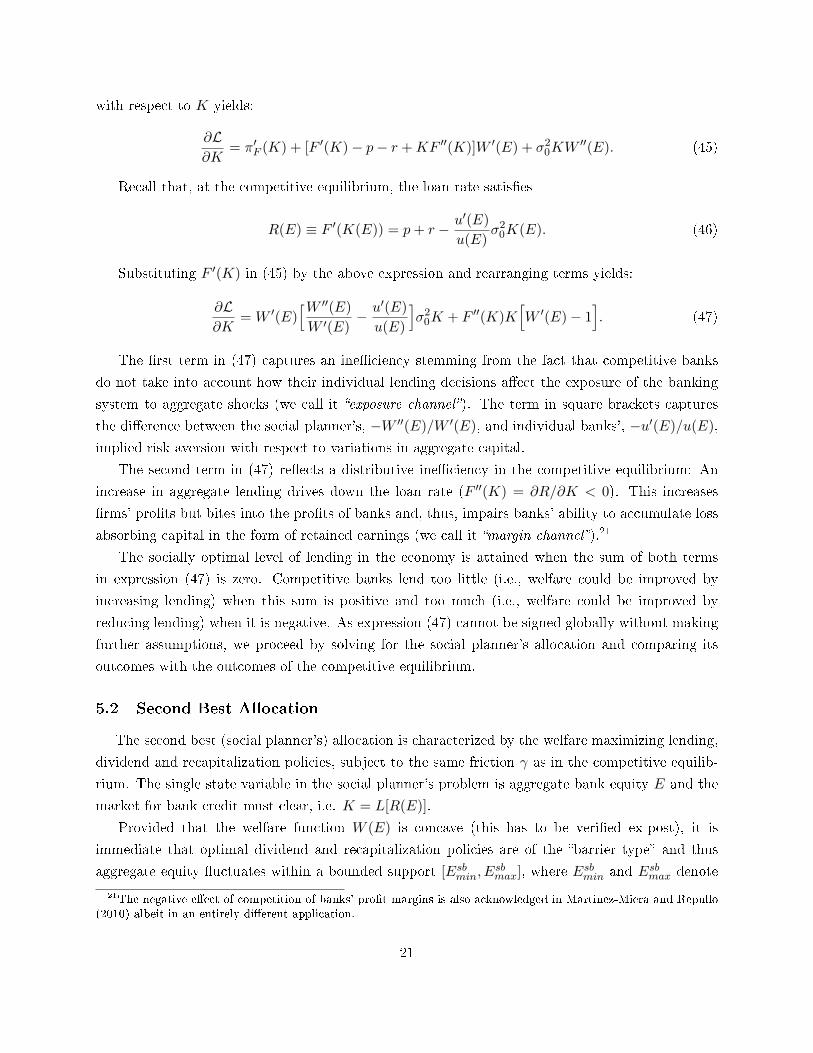
with respect to K yields:

∂L∂K

= π′F (K) + [F ′(K)− p− r +KF ′′(K)]W ′(E) + σ20KW

′′(E). (45)

Recall that, at the competitive equilibrium, the loan rate satis�es

R(E) ≡ F ′(K(E)) = p+ r − u′(E)

u(E)σ2

0K(E). (46)

Substituting F ′(K) in (45) by the above expression and rearranging terms yields:

∂L∂K

= W ′(E)[W ′′(E)

W ′(E)− u′(E)

u(E)

]σ2

0K + F ′′(K)K[W ′(E)− 1

]. (47)

The �rst term in (47) captures an ine�ciency stemming from the fact that competitive banks

do not take into account how their individual lending decisions a�ect the exposure of the banking

system to aggregate shocks (we call it �exposure channel�). The term in square brackets captures

the di�erence between the social planner's, −W ′′(E)/W ′(E), and individual banks', −u′(E)/u(E),

implied risk aversion with respect to variations in aggregate capital.

The second term in (47) re�ects a distributive ine�ciency in the competitive equilibrium: An

increase in aggregate lending drives down the loan rate (F ′′(K) = ∂R/∂K < 0). This increases

�rms' pro�ts but bites into the pro�ts of banks and, thus, impairs banks' ability to accumulate loss

absorbing capital in the form of retained earnings (we call it �margin channel�).21

The socially optimal level of lending in the economy is attained when the sum of both terms

in expression (47) is zero. Competitive banks lend too little (i.e., welfare could be improved by

increasing lending) when this sum is positive and too much (i.e., welfare could be improved by

reducing lending) when it is negative. As expression (47) cannot be signed globally without making

further assumptions, we proceed by solving for the social planner's allocation and comparing its

outcomes with the outcomes of the competitive equilibrium.

5.2 Second Best Allocation

The second best (social planner's) allocation is characterized by the welfare maximizing lending,

dividend and recapitalization policies, subject to the same friction γ as in the competitive equilib-

rium. The single state variable in the social planner's problem is aggregate bank equity E and the

market for bank credit must clear, i.e. K = L[R(E)].

Provided that the welfare function W (E) is concave (this has to be veri�ed ex-post), it is

immediate that optimal dividend and recapitalization policies are of the �barrier type� and thus

aggregate equity �uctuates within a bounded support [Esbmin, Esbmax], where Esbmin and Esbmax denote

21The negative e�ect of competition of banks' pro�t margins is also acknowledged in Martinez-Miera and Repullo(2010) albeit in an entirely di�erent application.

21

the recapitalization and the dividend distribution barriers, respectively. For E ∈ [Esbmin, Esbmax], the

social welfare function satis�es the following HJB equation:

ρW (E) = maxK≥0

F (K)−KF ′(K)+(rE +K[F ′(K)− p− r]

)W ′(E) +

σ20

2K2W ′′(E). (48)

Taking the �rst-order condition of the right-hand side of (48) with respect to K, and rearranging

terms shows that the second-best loan rate, Rsb(E), satis�es:

Rsb(E)− p− r = −W′′(E)

W ′(E)σ2

0Ksb(E)+

( 1

W ′(E)− 1)KsbF ′′(Ksb), (49)

where Ksb = L(Rsb). Given that W ′(Esbmax) = 1 and W ′′(Esbmax) = 0, it is easy to see that

Rsb(Esbmax) = p+ r, like in the competitive equilibrium.

Note that the above expression shares some similarities with the expression (22) in the compet-

itive equilibrium, with the notable distinction that the loan rate depends on the social implied risk

aversion with respect to variation in aggregate equity, −W ′′(E)/W ′(E), whereas in the competitive

equilibrium, it is driven by the private implied risk aversion −u′(E)/u(E). Moreover, there is an

additional term which is always positive or zero, as the (social) marginal value of earnings retained

in banks is weakly higher than the marginal value of instantaneously consumed �rms' pro�ts, i.e.,

W ′(E) ≥ 1.

The following proposition summarizes the characterization of the second best allocation.

Proposition 3 The Second Best allocation is characterized by the aggregate lending functionKsb(E) =

L(Rsb(E)), where Rsb(E) is implicitly given by (49). The welfare function Wsb(E) satis�es the ODE

ρWsb(E) = F (Ksb)−KsbF ′(Ksb)+(rE +Ksb[F ′(Ksb)− p− r]

)W ′sb(E) +

σ20

2[Ksb]2W ′′sb(E),

subject to the boundary conditions W ′sb(0) = W ′sb(Esbmax) − γ = 1. Banks distribute dividends when

Et reaches Esbmax = [W ′′sb]

−1(0) and recapitalize when Et hits zero.

To illustrate credit market ine�ciencies emerging in our model set-up, we resort to the numerical

example using a simple linear speci�cation of the demand for loans that is obtained from the one

introduced in (31) by setting β = 1.22

The left panel in Figure 3 shows that in the competitive equilibrium (CE), a poorly-capitalized

banking system lends more than under the second best (SB) allocation, which re�ects the pecuniary

externality in�icted by each bank on its competitors. The social planner internalizes this externality

and reduces the exposure to macro shocks (σ0K(E)) in the states of the world where the implied risk

aversion with respect to �uctuations in E is most severe (i.e., close to the recapitalization barrier

22Using a simple linear speci�cation of the loan demand allows us to compute the Second Best allocation withoutusing value-iteration algorithms.

22

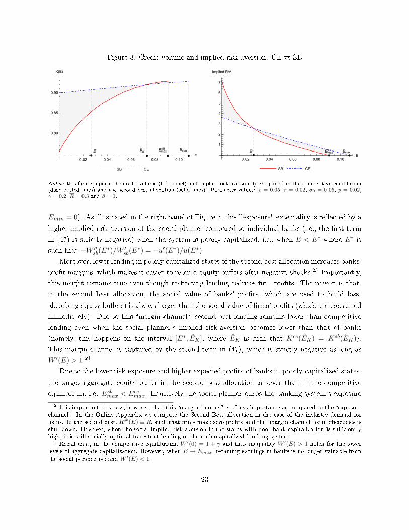
Figure 3: Credit volume and implied risk aversion: CE vs SB

0.02 0.04 0.06 0.08 0.10E

0.80

0.85

0.90

K(E)

SB CE

0.02 0.04 0.06 0.08 0.10E

1

2

3

4

5

6

7

Implied R/A

SB CE

EmaxSB EmaxE

KE* Emax

SB EmaxE*

Notes: this �gure reports the credit volume (left panel) and implied risk-aversion (right panel) in the competitive equilibrium(dash-dotted lines) and the second best allocation (solid lines). Parameter values: ρ = 0.05, r = 0.02, σ0 = 0.05, p = 0.02,γ = 0.2, R = 0.3 and β = 1.

Emin = 0). As illustrated in the right panel of Figure 3, this "exposure" externality is re�ected by a

higher implied risk-aversion of the social planner compared to individual banks (i.e., the �rst term

in (47) is strictly negative) when the system is poorly capitalized, i.e., when E < E∗ where E∗ is

such that −W ′′sb(E∗)/W ′sb(E∗) = −u′(E∗)/u(E∗).

Moreover, lower lending in poorly capitalized states of the second best allocation increases banks'

pro�t margins, which makes it easier to rebuild equity bu�ers after negative shocks.23 Importantly,

this insight remains true even though restricting lending reduces �rm pro�ts. The reason is that,

in the second best allocation, the social value of banks' pro�ts (which are used to build loss-

absorbing equity bu�ers) is always larger than the social value of �rms' pro�ts (which are consumed

immediately). Due to this �margin channel�, second-best lending remains lower than competitive

lending even when the social planner's implied risk-aversion becomes lower than that of banks

(namely, this happens on the interval [E∗, EK ], where EK is such that Kce(EK) = Ksb(EK)).

This margin channel is captured by the second term in (47), which is strictly negative as long as

W ′(E) > 1.24

Due to the lower risk-exposure and higher expected pro�ts of banks in poorly-capitalized states,

the target aggregate equity bu�er in the second best allocation is lower than in the competitive

equilibrium, i.e. Esbmax < Ecemax. Intuitively the social planner curbs the banking system's exposure

23It is important to stress, however, that this �margin channel� is of less importance as compared to the �exposurechannel�. In the Online Appendix we compute the Second Best allocation in the case of the inelastic demand forloans. In the second best, Rsb(E) ≡ R, such that �rms make zero pro�ts and the �margin channel� of ine�ciencies isshut down. However, when the social implied risk aversion in the states with poor bank capitalization is su�cientlyhigh, it is still socially optimal to restrict lending of the undercapitalized banking system.

24Recall that, in the competitive equilibrium, W ′(0) = 1 + γ and thus inequality W ′(E) > 1 holds for the lowerlevels of aggregate capitalization. However, when E → Emax, retaining earnings in banks is no longer valuable fromthe social perspective and W ′(E) < 1.

23

to macro shocks when they are most harmful (i.e. when implied risk-aversion is most severe), while

individual banks fail to e�ciently control aggregate risk. As a result, the critical capital bu�er at

which the social planner no longer requires a lending premium is lower than the one at which this

is the case for individual banks (recall that Rce(Ecemax) = Rsb(Esbmax) = p+ r). Hence, if the target

aggregate equity bu�er Ecemax is su�ciently high in the competitive set-up, banks are e�ectively more

risk-averse than the social planner and, thus, lending is ine�ciently low in the vicinity of Ecemax.25

6 Impact of capital regulation

The evidence of welfare distortions in the competitive equilibrium calls for macroprudential

regulation. Our objective in this section is to investigate the impact of capital regulation on bank

policies and the long run behavior of the economy.

6.1 Regulated equilibrium

We consider a requirement for each bank to �nance at least fraction Λ of its risky loans by equity,

i.e.,

et ≥ Λkt. (50)

Facing a binding capital requirement, banks can either issue new equity or de-lever by reducing

lending and debt. We show below that, compared to the unregulated case, banks on the one hand

recapitalize earlier (i.e., EΛmin > 0) and on the other hand reduce lending when the constraint is

binding but, for precautionary reasons, also when it is slack. As in the unregulated case, individual

banks choose lending, recapitalization and dividend policies subject to the regulatory constraint to

maximize the market value of equity:26

vΛ(e, E) ≡ euΛ(E) = maxkt≤ e

Λ,dδt,dit

E[∫ +∞

0e−ρt (dδt − (1 + γ)dit)|e0 = e, E0 = E

]. (51)

Recall that in the unregulated equilibrium bank lending is always strictly positive and banks

recapitalize only when equity is completely depleted. Capital regulation must therefore bind for

su�ciently low levels of capital. In this case, lending is determined by the binding constraint (50).

If it is slack, the interior level of lending must satisfy an individual rationality condition equivalent

to (22) in the unregulated case. In both cases, the relation between equilibrium lending and loan

rate is pinned down by the market clearing condition.

25Note that the regulatory restrictions on lending changes the marginal value of bank equity. Namely, in the socialplanner's allocation, u(E) spikes above 1 + γ for the low levels of aggregate bank capital. This implies that, if bankshareholders were free to choose the recapitalization barrier, they would recapitalize at a strictly positive level ofaggregate capital.

26Note that homotheticity is not a�ected by the considered form of regulation.

24

Proposition 4 For all Λ ∈ (0, 1], there exists a unique regulated equilibrium, where banks' market

to book value of equity satis�es the HJB equation

(ρ− r)uΛ(E) =[rE + L(R(E))(R(E)− p− r)

]u′Λ(E) +

σ20L(R(E))2

2u′′Λ(E)

+1

Λ

[(R(E)− p− r)uΛ(E) + σ2

0L(R(E))u′Λ(E)],

(52)

for E ∈ [EΛmin, E

Λmax], subject to the boundary conditions uΛ(EΛ

max) = uΛ(EΛmin) − γ = 1 and

u′Λ(EΛmax) = u′Λ(EΛ

min) = 0. Furthermore, there exists a unique threshold EΛc such that

a) for E ∈ [EΛmin, E

Λc ] the regulatory constraint binds, i.e., K(E) = E/Λ. The equilibrium loan rate

is explicitly given by the market clearing condition:

R(E) = L−1(E/Λ), (53)

where L−1 is the inverse function of the loan demand. The evolution of aggregate bank capital is

given by:dEtEt

= rEdt+1

Λ

((R(Et)− p− r)dt− σ0dZt

), E ∈ (EΛ

min, EΛc ).

b) for Et ∈ (EΛc , E

Λmax] the regulatory constraint is slack. The equilibrium loan rate satis�es the

�rst-order di�erential equation (28) subject to the boundary condition R(EΛc ) = L−1[EΛ

c /Λ].

Finally, there exists a unique threshold Λ∗ ∈ (0, 1) such that EΛc = EΛ

max, i.e., the constraint binds

for all E ∈ [EΛmin, E

Λmax], when Λ > Λ∗.

Note that, when the constraint is not binding, the equilibrium loan rate is determined by the

same condition as in the unregulated equilibrium (see condition (22)), so that the term in square

brackets in the second line of HJB (52) vanishes. If the constraint is binding, however, this term is

strictly positive and can be interpreted as the shadow costs associated with the constraint.

We turn to the results of our numerical analysis to illustrate the impact of minimum capital

regulation on bank policies, systemic stability and the distribution of welfare across states.27

6.2 Dividend and recapitalization policies

Figure 4 illustrates the impact of the minimum capital ratio on the optimal recapitalization and

dividend policies of banks. In contrast to the unregulated case, it is no longer optimal to postpone

recapitalizations until equity is fully depleted (EΛmin > 0). This is an immediate consequence of the

fact that banks are allowed to lend at most fraction 1/Λ of their equity, so that a bank with zero

27In Appendix we provide a detailed description of the computational procedure implemented to solve for theregulated equilibrium.

25

equity and, thus, zero loans, would be permanently out of business. Therefore, as illustrated in

Figure 4, the recapitalization boundary EΛmin is strictly increasing in the minimum capital ratio Λ.

When the regulator imposes a higher minimum capital ratio, Λ, the dividend boundary grows

at a higher rate than the recapitalization boundary, such that the maximum loss absorbing capacity

of the banking system, EΛmax − EΛ

min, expands as well. To understand this e�ect, note �rst that,

as long as the constraint does not bind globally (Λ ≤ Λ∗), banks distribute dividends when the

marginal loan is no longer pro�table, i.e. the equilibrium loan rate at the dividend boundary EΛmax

equals the unconditional default rate (RΛmin = p + r). As regulation reduces the supply of bank

loans, banks' pro�t margins increase at any given level of aggregate capital, which in turn drives up

EΛmax. This e�ect is even more pronounced for su�ciently high minimum capital ratios (Λ > Λ∗),

where the constraint binds globally and RΛmin > p+ r.

Figure 4: Minimum capital requirements and bank policies

20 40 60 80 100Λ,%

0.2

0.4

0.6

0.8

E

EminΛ Ec

Λ EmaxΛ

20 40 60 80 100Λ,%

0.05

0.10

0.15

R

RmaxΛ Rmin

Λ

Impact of capital regulationon the maximum loan rate Rmax

Λ* = 44%

Emaxr + p

Notes: this �gure illustrates the impact of minimum capital ratios on the optimal dividend and recapitalization policies. Thedashed line indicates the values of the maximum level of aggregate capital in the absence of regulation (Emax). The shadedarea marks the states of E in which the regulatory constraint is binding. For Λ > Λ∗ (Λ∗ = 44% in this numerical example),the regulatory constraint is binding for any E ∈ [EΛ

min, EΛmax]. Parameter values: ρ = 0.05, r = 0, σ0 = 0.05, p = 0.02, γ = 0.2,

R = 0.3, β = 1.

6.3 Loan rates

Figure 5 illustrates the impact of a minimum capital ratio on the minimum and maximum

levels of the equilibrium loan rate. In particular, it shows that, as long as the constrained and

unconstrained region coexist (in this numerical example this occurs for any Λ < Λ∗) the minimum

loan rate RΛmin remains at its frictionless level p + r. For capital ratios that make the regulatory

constraint binding for any level of aggregate capital, the minimum loan rate is determined by the

binding regulatory constraint and thus stays strictly above its frictionless level.

It is also worthwhile to note that for Λ → 0, the equilibrium loan rate at the recapitalization

boundary RΛmax (indicated by the solid line) does not converge to its unregulated counterpart Rmax

26

(the dashed line). The reason is that the loan rate has to ensure market clearing and, thus, a capital

constraint that binds over a nonempty (albeit small) region drives up the market clearing loan rate

by discrete amount. As a result, even a tiny minimum capital ratio leads to signi�cant increase in

RΛmax.

Figure 5: Minimum capital requirements and loan rates

20 40 60 80 100Λ,%

0.2

0.4

0.6

0.8

E

EminΛ Ec

Λ EmaxΛ

20 40 60 80 100Λ,%

0.05

0.10

0.15

R

RmaxΛ Rmin

Λ

Impact of capital regulationon the maximum loan rate Rmax

Λ* = 44%

Emax p + r

Notes: this �gure illustrates the impact of minimum capital ratios on the equilibrium loan rates. The dashed line indicates thevalues of the maximum loan rate in the absence of regulation (Rmax). For Λ > Λ∗ (Λ∗ = 44% in this numerical example), theregulatory constraint is binding for any level of aggregate capital and thus RΛ

min > p + r. Parameter values: ρ = 0.05, r = 0,

σ0 = 0.05, p = 0.02, γ = 0.2, R = 0.3, β = 1.

6.4 Lending

The direct impact of the minimum capital ratio on lending is illustrated in Figure 6.

Consider �rst a relatively mild minimum capital ratio of, say 3%, which in fact leads to a

signi�cant reduction in exposure when the constrained is binding (i.e., when the system is poorly

capitalized). Interestingly, the e�ect of the minimum capital requirements propagates over the

unconstrained region. This result is driven by the banks' precautionary motive: anticipating a

potentially binding constraint in the future, banks also reduce lending when the constraint is slack,

albeit less severely. Thus, while mitigating ine�ciencies (excessive lending) in poorly capitalized

states, the constant minimum capital ratio exacerbates ine�ciencies (insu�cient lending) in good

states.

Above some critical level of Λ, further increases in capital requirements will lead to ine�ciently

low lending for all feasible levels of aggregate capitalization. Indeed, upon raising the minimum

capital ratio to 10%, the region in which the constraint binds expands (cf. the shaded area in

Figure 4), and lending in the constrained region declines further, falling far below the second best

level.28 Moreover, with a stricter minimum capital ratio also the precautionary motive and, thus,

28Note that banks react to the stricter regulation by increasing EΛmin, yet, not su�ciently to maintain the same

level of lending. Therefore, RΛmax, which is represented by the solid line in Figure 5, is strictly increasing in Λ.

27

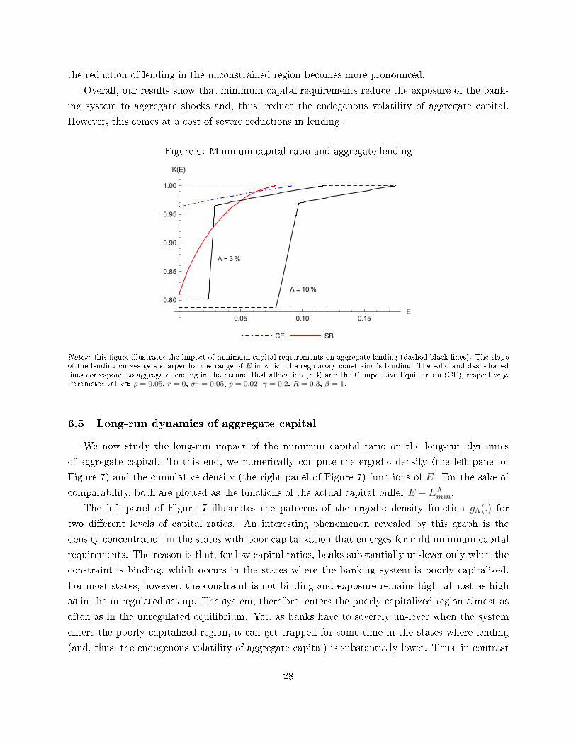
the reduction of lending in the unconstrained region becomes more pronounced.

Overall, our results show that minimum capital requirements reduce the exposure of the bank-

ing system to aggregate shocks and, thus, reduce the endogenous volatility of aggregate capital.

However, this comes at a cost of severe reductions in lending.

Figure 6: Minimum capital ratio and aggregate lending

0.05 0.10 0.15E

0.80

0.85

0.90

0.95

1.00

K(E)

CE SB

Λ = 3%

Λ = 10%

Notes: this �gure illustrates the impact of minimum capital requirements on aggregate lending (dashed black lines). The slopeof the lending curves gets sharper for the range of E in which the regulatory constraint is binding. The solid and dash-dottedlines correspond to aggregate lending in the Second Best allocation (SB) and the Competitive Equilibrium (CE), respectively.Parameter values: ρ = 0.05, r = 0, σ0 = 0.05, p = 0.02, γ = 0.2, R = 0.3, β = 1.

6.5 Long-run dynamics of aggregate capital

We now study the long-run impact of the minimum capital ratio on the long-run dynamics

of aggregate capital. To this end, we numerically compute the ergodic density (the left panel of

Figure 7) and the cumulative density (the right panel of Figure 7) functions of E. For the sake of

comparability, both are plotted as the functions of the actual capital bu�er E − EΛmin.

The left panel of Figure 7 illustrates the patterns of the ergodic density function gΛ(.) for

two di�erent levels of capital ratios. An interesting phenomenon revealed by this graph is the

density concentration in the states with poor capitalization that emerges for mild minimum capital

requirements. The reason is that, for low capital ratios, banks substantially un-lever only when the

constraint is binding, which occurs in the states where the banking system is poorly capitalized.

For most states, however, the constraint is not binding and exposure remains high, almost as high

as in the unregulated set-up. The system, therefore, enters the poorly capitalized region almost as

often as in the unregulated equilibrium. Yet, as banks have to severely un-lever when the system

enters the poorly capitalized region, it can get trapped for some time in the states where lending

(and, thus, the endogenous volatility of aggregate capital) is substantially lower. Thus, in contrast

28

to the models in the similar style (see e.g. Brunnermeier and Sannikov (2014) and Phelan (2015)),

in our model the bimodal density pattern can emerge only due to the impact of regulation, whereas,

in the unregulated framework, the ergodic density is unimodal for the whole range of acceptable

parameter values.

For su�ciently high minimum capital ratios exposure to aggregate shocks (lending) is also sub-

stantially reduced when the system is well capitalized. Furthermore, cutting on lending boosts

banks' expected pro�ts, and, thus, improves the banking system's capacity to accumulate capital.

As a result of these two e�ects, the spike in the density pattern disappears and the density concen-

tration occurs only in highly-capitalized states. Thus, enhancing capital requirements makes the

banking system more stable.

This feature is also illustrated in the right-hand side panel of Figure 7, which reports the banking

system's stability, measured by the average time to recapitalization (T γ(E)) (see Appendix for

the computational details). As stability is strictly increasing in the minimum capital ratio Λ, for

su�ciently high capital ratios the banking system becomes even more stable than in the second best

allocation. This, however, comes at the cost of substantial reductions in lending and, thus, output.

Figure 7: The ergodic density of E and average time to recapitalization

0.02 0.04 0.06 0.08 0.10E - Emin

4

6

8

10

12

14

g(E)

CE SB Λ>0

5 10 15 20Λ

1

2

3

4

5

6

7

Tγ(E)

CE SB Λ>0

Λ = 25%

Λ = 3%

Notes: this �gure illustrates the impact of a constant minimum capital ratio on the ergodic density of E (left panel) and averagetime to recapitalization. Parameter values: ρ = 0.05, r = 0, σ0 = 0.05, p = 0.02, γ = 0.2, R = 0.3, β = 1.

7 Conclusion

This paper develops a general equilibrium model of commercial banking, in which banks satisfy

households' needs for safe deposits and channel funds to the productive sector. Bank capital plays

the role of a loss-absorbing bu�er that insulates banks from the need to undertake costly recapital-

izations too often. In our model, the aggregate level of bank capitalization drives the cost and the

volume of lending. Speci�cally, we establish a negative relation between the equilibrium loan rate

29

and the level of aggregate bank capital that is supported by data. The competitive equilibrium is

not constrained e�cient because of a pecuniary externality which leads to excessive lending in the

states with poor bank capitalization and insu�cient lending in well-capitalized states. Minimum

capital requirements curb lending, which enhances stability of the banking system.

Our model is a �rst step toward the analysis of bank regulation policies in a fully speci�ed

dynamic model. Several extensions appear important. First, in future research, we plan to explore

the welfare e�ects of �countercyclical� capital regulation in the extended version of our model that

explicitly accounts for business cycles. Second, introducing market activities such as investment

in securities in addition to the current focus on commercial banking activities (deposit taking and

lending) might be important to understand the dynamics of endogenous risk. Finally, in this paper

we have focused on the scenario in which private bank recapitalizations prevent systemic crises

from happening. A potential direction of further investigations would be to explore the alternative

scenarios in which shareholders do not have incentives to inject new capital, and public authorities

are forced to intervene.

30

Appendix

I. Proofs

Proof of Proposition 1. Omitted.

Proof of Proposition 2. By the standard dynamic programming arguments, shareholder valuev(e, E) must satisfy the Bellman equation:29

ρv = maxk≥0,dδ≥0,di≥0

{dδ(1− ve)− di(1 + γ − ve)

+[re+ k(R(E)− p− r)

]ve + kK(E)σ2

0veE +k2σ2

0

2vee

+[rE +K(E)(R(E)− p− r)

]vE +

σ20K

2(E)

2vEE

}.

(I.1)

Using the fact that v(e, E) = eu(E), one can rewrite the Bellman equation (I.2) as follows:

(ρ− r)u(E) = maxdδ≥0

{dδe

[1− u(E)]}−max

di≥0

{die

[1 + γ − u(E)]}

+ maxk≥0

{ke

[(R(E)− p− r)u(E) + σ2

0K(E)u′(E)]}

+(rE +K(E)[R(E)− p− r]

)u′(E) +

σ20K

2(E)

2u′′(E).

(I.2)A solution to the maximization problem in k only exists when

u′(E)

u(E)≤ −R(E)− p− r

σ20K(E)

, (I.3)

with equality when k > 0.Assuming that R(E) ≥ p + r (which is veri�ed ex-post), it follows from the above expression

that u(E) is a decreasing function of E. Then, the optimal payout policy maximizing the right-handside of (I.2) is characterized by a critical barrier Emax satisfying

u(Emax) = 1, (I.4)

and the optimal recapitalization policy is characterized by a barrier Emin such that

u(Emin) = 1 + γ. (I.5)

In other words, dividends are only distributed when Et reaches Emax, whereas recapitalizationoccurs only when Et reaches Emin. Given (I.3), (I.4), (I.5) and k > 0, it it easy to see that, in theregion E ∈ (Emin, Emax), market-to-book value u(E) satis�es:

(ρ− r)u(E) =[rE +K(E)(R(E)− p− r)

]u′(E) +

σ20K

2(E)

2u′′(E). (I.6)

29For the sake of space, we omit the arguments of function v(e, E).

31

Note that, at equilibrium, K(E) = L(R(E)). Taking the �rst derivative of (I.3), we can computeu′′(E). Inserting u′′(E) and u′(E) into (I.6) and rearranging terms yields:

R′(E) = − 1

σ20

2(ρ− r)σ20 + (R(E)− p− r)2 + 2(R(E)− p− r)rE/L(R(E))

L(R(E))− (R(E)− p− r)L′(R(E)). (I.7)

Since L′(R(E)) < 0, it is clear that R′(E) < 0 if R(E) > p+ r. To verify that R(E) > p+ r forany E ∈ [Emin, Emax), it is su�cient to show that Rmin ≡ R(Emax) ≥ p+ r.

To obtain Rmin, letV (E) ≡ Eu(E)

denote the market value of the entire banking system. At equilibrium, dividends are distributedwhen the marginal value of bank capital equals the marginal value of dividends, which implies

V ′(Emax) = u(Emax) + Emaxu′(Emax) = 1.

Similarly, recapitalizations take place when the marginal value of bank capital equals themarginal costs of recapitalizing the banks, which implies

V ′(Emin) = u(Emin) + Eminu′(Emin) = 1 + γ.

Given (I.4) and (I.5), it must hold that30

u′(Emax) = 0,

andEmin = 0.

Inserting u′(Emax) = 0 into the binding condition (I.3) immediately shows that Rmin = p + r,so that R(E) > p+ r for any E ∈ [Emin, Emax).

Hence, for any given Emax, the loan rate R(E) can be computed as a solution to the di�erentialequation (I.7) with the boundary condition R(Emax;Emax) = p+ r.

To obtain Emax, we use the fact that individual banks' optimization with respect to the recap-italization policy implies u(0) = 1 + γ. Integrating equation (I.3) in between Emin = 0 and Emax,while taking into account the condition u(Emax) = 1, yields an equation that implicitly determinesEmax:

u(Emax)exp(∫ Emax

0

R(E;Emax)− p− rσ2

0L(R(E;Emax))dE)

︸ ︷︷ ︸u(0)

= 1 + γ. (I.8)

Note that, since R(E;Emax) is increasing with Emax, the right-hand side of Equation (I.8)increases with Emax. When the left-hand side of equation (I.8) is larger than 1+γ when Emax →∞,it has the (unique) solution.31 Q.E.D.

Proof of Proposition 3. For any given barriers Esbmin and Esbmax, solving for the second best

30As we show in Appendix B, these properties can be alternatively established by looking at the limit of thediscrete-time equilibrium characterization for h→ 0.

31Throughout the paper we focus on this case. In the alternative case all banks default simultaneously when Etfalls to zero.

32

allocation requires solving for the functions Rsb(E) andW (E) that simultaneously satisfy equations(49) and (42), subject to the boundary conditions W ′(Esbmin) = W ′(Esbmax) − γ = 1. From theconcavity of the welfare function it immediately follows that Esbmin = 0, whereas the optimal targetlevel of equity Esbmax must satisfy the super-contact condition W ′′(Esbmax) = 0. Q.E.D.Proof of Proposition 4. Consider the shareholders' maximization problem stated in (51). Bythe standard dynamic programming arguments and the fact that vΛ(e, E) = euΛ(E), where uΛ(E)satis�es the following Bellman equation:

(ρ− r)uΛ(E) = maxdδ≥0,di≥0

{dδe

[1− uΛ(E)]− di

e[1 + γ − uΛ(E)]

}+

+ max0<k≤e/Λ

{ke

[(R(E)− p− r)uΛ(E) + σ20K(E)u′Λ(E)]

}+

+(rE +K(E)[R(E)− p− r]

)u′Λ(E) +

σ20K

2(E)

2u′′Λ(E).

(I.9)A solution to (I.9) exists only if K(E) ≤ E/Λ, and

B(E) :=R(E)− p− rσ2

0K(E)≥ −

u′Λ(E)

uΛ(E)≡ y(E), (I.10)

with equality when K(E) < E/Λ.The optimal dividend and recapitalization policies are characterized by barriers EΛ

max and EΛmin

such that uΛ(EΛmax) = 1 and uΛ(EΛ

min) = 1 + γ. Moreover, by the same reason that in theunregulated equilibrium, it must hold that

EΛmaxu

′Λ(EΛ

max) = 0,

andEΛminu

′Λ(EΛ

min) = 0.

From the �rst equation we immediately have u′Λ(EΛmax) = 0. The implication of the second

equation is less trivial. Recall that in the unregulated equilibrium, we had Emin = 0. However,under capital regulation, this is no longer possible, as K(E) = E/Λ on the constrained region andthus equation (I.9) could not hold when E → 0. Therefore, it must be that u′Λ(EΛ

min) = 0.With the conjecture that there exists some critical threshold EΛ

c such that the regulatory con-straint is binding for E ∈ [EΛ

min, EΛc ] and is slack for E ∈ [EΛ

c , EΛmax], equation (I.9) can be rewritten

as the �rst-order di�erential equation:32

ρ− r = −µ(E)y(E) +σ2

0K2(E)

2[y2(E)− y′(E)] +

[R(E)− p− r − σ20K(E)y(E)]

Λ(I.11)

where µ(E) denotes the drift of aggregate capital (banks' expected pro�ts):

µ(E) = rE +K(E)[R(E)− p− r],32Note that the last term in the right-hand side of equation (I.11) vanishes when E ∈ [EΛ

min, EΛc ], because condition

(I.10) holds with equality.

33

the volume of lending K(E) satis�es

K(E) =

{E/Λ, E ∈ [EΛ

min, EΛc ]

L(R(E)), E ∈ (EΛc , E

Λmax],

(I.12)

and the loan rate R(E) is given by

R(E) =

{L−1(E/Λ), E ∈ [EΛ

min, EΛc ]

R′(E) = H(R(E)), R(EΛc ) = L−1(EΛ

c /Λ), E ∈ (EΛc , E

Λmax],

(I.13)

where H(R(E)) is de�ned in (28) and L−1 is the inverse function of the demand for loans.Note that the value-matching condition for the loan rate function at EΛ

c is implied by the fact thefunction u(E) and its �rst derivative are continuous functions of their argument and the constraint(I.10) holds with equality at EΛ

c .The critical threshold EΛ

c must satisfy equation

y(EΛc ) = B(EΛ

c ).

If y(E) < B(E) for any E ∈ [EΛmin, E

Λmax], then the regulatory constraint is always binding and

y(E) satis�es equation (I.11) with EΛc = EΛ

max. The condition u′Λ(EΛmin) = 0 yields the bound-

ary condition y(Emin) = 0. Similarly, the condition u′Λ(EΛmax) = 0 translates into the boundary

condition y(Emax) = 0. Q.E.D.

II. Solving for the regulated equilibrium

a) Numerical procedure

This numerical algorithm solving for the competitive equilibrium with minimum capital regulationcan be implemented with the Mathematica software:33

• Pick a candidate value EΛmin.

• Assume that the regulatory constraint always binds. Solve ODE (I.11) for y(E) under theboundary condition y(Emin) = 0.

• Compute a candidate value EΛmax such that satis�es equation y(EΛ

max) = 0.

• Check whether y(EΛmax) ≤ B(EΛ

max).

• Conditional on the results of the previous step, one of the two scenarios is possible:

a) if y(EΛmax) ≤ B(EΛ

max), then the regulatory constraint is always binding for a given Λ,i.e., there is a single �constrained� region. In this case market-to-book value uΛ(EΛ

min)can be computed according to

uΛ(EΛmin) = uΛ(EΛ

max)exp(∫ EΛ

max

EΛmin

y(E)dE)

= exp(∫ EΛ

max

EΛmin

y(E)dE).

33In all computations Λ is taken as a parameter.

34

b) observing y(EΛmax) > B(EΛ

max) means that, for given EΛmin, the constrained and uncon-

strained regions coexist. To �nd the critical level of aggregate equity EΛc above which

the regulatory constraint is slack, one needs to solve the following equation:

y(EΛc ) = B(EΛ

c ).

� using EΛc and (I.13), de�ne the function R(E) for E > EΛ

c ;

� compute a new candidate for the dividend boundary, EΛmax, such that B(EΛ

max) = 0(note that this is equivalent to solving equation R(EΛ

max) = p);

� compute the market-to-book value uΛ(EΛmin) according to:

uΛ(EΛmin) = exp

(∫ EΛc

EΛmin

y(E)dE)exp(∫ EΛ

max

EΛc

B(E)dE).

• If uΛ(EΛmin) = 1 + γ, then EΛ

min = EΛmin, E

Λmax = EΛ

max (or EΛmax if 2 regions) and EΛ

c = EΛc

(if 2 regions). Otherwise, pick a di�erent EΛmin, repeat the procedure from the beginning.

b) Ergodic density

Since all variables of interest are the deterministic functions of E, we directly use the ergodic densityof aggregate bank capitalization in order to compute their average values. Given the dynamics ofE de�ned in the Proposition 4 , the ergodic density function of E in the regulated competitiveequilibrium can be computed according to:

gΛ(E) =CΛ

σ20K

2(E)exp(∫ EΛ

max

EΛmin

2[rE +K(E)(R(E)− p− r)]σ2

0K2(E)

dE),

where K(E) and R(E) are de�ned in (I.12) and (I.13) respectively, and the constant CΛ is such

that∫ EΛ

max

EΛmin

gΛ(E)dE = 1.

c) Expected time to reach the recapitalization barrier

Let T γ(E) denote the expected time it takes to reach the recapitalization boundary EΛmin starting

from any E ≥ EΛmin. Since t + T γ(Et) is a martingale, function T γ(E) satis�es the following

di�erential equation:

[K(E)σ0]2

2T′′γ(E)+

[rE +K(E)(R(E)− p− r)]T ′γ(E) + 1 = 0, (EΛ

min, EΛmax),

where functions K(E) and R(E) are de�ned in (I.12) and (I.13) respectively.The above equation is subject to the following two boundary conditions: T γ(EΛ

min) = 0 (i.e., it

takes no time to reach EΛmin from EΛ

min), and T′γ(EΛ

max) = 0, which emerges due to the re�ectionproperty of aggregate equity. To measure the impact of minimum capital requirements on �nancialstability in Section 6, for each level of Λ, we compute T γ(E) - the expected time to reach therecapitalization boundary EΛ

min starting from the long-run average level of aggregate equity, E.

35

III. Empirical analysis

This Appendix presents a simple assessment of the consistency of the key predictions of ourmodel with the data. As stated in Section 3.3, our model delivers two key predictions: bank loanrates and the ratio of market-to-book equity are (weakly) decreasing functions of aggregate bankequity. We assess these predictions by estimating panel regressions between measures of bank grossreturns on earning assets, the ratio of market-to-book equity, and aggregate bank equity. We usea large bank-level panel dataset. Its use, and the attendant heterogeneity of the data for banksbelonging to a speci�c country group, place a strong consistency requirement on the predictions ofour model, which is constructed under the simplifying assumption of homogeneous banks.

Our results indicate that the key predictions of our model are not rejected by standard sta-tistical tests, are consistent with a large variety of country circumstances, and are robust to dataheterogeneity owing to our use of a �rm-level panel dataset.

a) Data and statistics

The data consists of consolidated accounts and market data for panels of publicly traded banks in43 advanced and emerging market economies for the period 1992-201234 taken from the Wordscopedatabase retrieved from Datastream.35 The sample is split into four sub-samples: U.S. banks;Japanese banks; banks in advanced economies (excluding the U.S. and Japan); banks in emergingmarket economies. Table 2 summarizes the de�nitions of the variables considered.

Table 2: De�nition of variables

Identi�er Variable Measurement

ret bank gross return on assets total interest income/earning assetsmtb market-to-book equity ratio market equity/book equitylogta bank size Log(assets)loanasset % of loans to assets total loans/total assetsbequity bank book equity bank book equitynpl non-performing loans non-performing loans in % of total assetsTBE total bank equity sum of bequity

Note that bank gross return on assets include revenues accruing from investments other thanloans; however, in the analysis below we will condition our estimates on asset composition usingthe % of loans to assets as a bank control. Furthermore, total bank equity is the sum of the equityof banks belonging to a particular country: this amounts to assuming that the relevant bankingmarket is the country. All other variables are exact empirical counterparts of the variables de�nedin the model.

34We do not include the 80s in our time period because of a low number of observations.35The Standard Industrial Classi�cation (SIC) System is used to identify the types of �nancial institutions included

in the sample, which are: National Commercial Banks (6021), State Commercial Banks (6022), Commercial BanksNot Elsewhere Classi�ed (6029), Savings Institution Federally Chartered (6035), Savings Institutions Not FederallyChartered (6036). In essence, the sample includes all publicly quoted depository institutions in the database. Thispanel dataset is unbalanced due to mergers and acquisitions, but all banks active in each period are included in thesample to avoid survivorship biases.

36

Table 3 reports sample statistics (Panel A) and some (unconditional) correlations (Panel B).Note that the correlations between bank returns, the market-to-book equity ratio, and total bankequity are negative and signi�cant. However, we wish to gauge conditional correlations, to whichwe now turn.

b) Panel regressions

We test whether there exists a negative conditional correlation between bank returns, market-to-book equity and total bank equity by estimating panel regressions with Yit ∈ (ret,mtb) as thedependent variable of the form:

Yit = α+βEt−1 +γ1bequityit−1 +γ2Logtait−1 +γ3loanassetit−1 +γ4nplt−1 +γ5Timedummyit+ εit.(D1)

All variables are lagged to mitigate potential endogenity problems. Model (D1) is used for theUS and Japan samples, while we add to Model (D1) country speci�c e�ects in the estimation forthe advanced economies and emerging market samples. Our focus in on the coe�cient β. Bankspeci�c e�ects are controlled for by the set of four variables (bequity, logta, loanasset, npl), wherenpl proxies risk in the bank's loan portfolio. The variable Timedummy denotes time dummies forthe US and Japan sample, and country-time dummies for the advanced economies and emergingmarkets samples: these dummy variables control for all time-varying country speci�c e�ects.

Table 4 reports the results. The coe�cient β is negative and (strongly) statistically signi�cantin all regressions. The quantitative impact of changes in total bank equity on both bank returnsand the market-to-book ratio is substantial as well. For example, a one standard deviation increasein total book equity (TBE) entails about 1.5 percentage point reduction in the loan rate. Thus, weconclude that the two key predictions of our model are consistent with the data.

Online Appendix

A. Discrete-time dynamic model

A.1. Competitive equilibrium in the dynamic discrete-time model

In this Appendix we develop a discrete-time dynamic model and show that, when the length oftime periods tends to zero, the outcomes of this model converges to the outcomes of the continuous-time model.

Let h denote the length of each time period. We work with the particular speci�cation of the�rms' default probability which allows the convergence to the di�usion process in the continuous

37

Table3:

Sam

plestatistics

andunconditional

correlations

PanelA:Sample

Statistics

US

Japan

Advanced(ex.USandJapan)

Emerging

Variable

Obs.

Mean

Std.Dev.

Obs.

Mean

Std.Dev.

Obs.

Mean

Std.Dev.

Obs.

Mean

Std.Dev.

ret

10213

6.49

1.57

2116

3.18

1.66

4779

7.34

4.09

3015

9.99

5.01

mtb

9542

1.42

0.71

2151

1.19

0.64

4788

1.4

0.85

2914

1.61

0.99

logta

10991

13.54

1.65

2342

17.12

1.22

5148

16.26

2.39

3473

15.65

1.94

loanasset

10812

65.96

13.42

2091

68.25

9.98

4572

70.38

16.53

3074

66.43

15.74

bequity(U

S$billion)

10923

0.98

9.19

2318

2.83

7.61

5133

5.23

14.16

3419

2.87

11.49

npl

10299

1.59

2.68

1770

4.11

2.89

2710

3.37

5.36

1937

5.92

8.78

TBE(U

S$billion)

16742

486.69

352.6

3061

297.38

108.18

7185

59.77

76.73

5696

35.65

108.21

PanelB:Correlations

ret

mtb

logta

ret

mtb

logta

ret

mtb

logta

ret

mtb

logta

mtb

0.23

68∗

10.5

481∗

1−

0.0

179

10.0

581∗

1

logta

−0.

2101

∗0.

2302

∗1

0.1220∗

0.2

694∗

1−

0.2

597∗

0.1992∗

1−

0.3720∗

0.0

909∗

1

TBE

−0.

7703

∗−

0.35

57∗

0.23

00∗

−0.

1764∗−

0.3131∗

0.1456∗

−0.3

283∗−

0.0

938∗

0.3128∗

−0.

1974∗−

0.0535∗

0.3772∗

Notes:∗indicatessigni�cance

at

5%

level.

38

Table4:

Panelregressions

US

Japan

Advanced(ex.USandJapan)

Emerging

(1)

(2)

(3)

(4)

(5)

(6)

(7)

(8)

Explanatory

variables

ret

mtb

ret

mtb

ret

mtb

ret

mtb

TBE

−0.

0041

6∗∗

∗−

0.0

0013

9∗∗

∗−

0.0124∗

∗∗−

0.00466∗∗

∗−

0.0123∗

∗∗−

0.0

0374∗∗

∗−

0.0

0280∗∗

∗−

0.0

0215∗∗

∗

[0.0

0][0.0

0][0.0

0]

[0.0

0]

[0.0

0]

[0.0

0]

[0.0

0]

[0.0

0]

bequity

0.00

232∗∗

−0.

0094

5∗∗∗

0.0

254∗∗

∗−

0.00316∗

0.0117∗∗

∗−

0.0

0113∗

0.0167∗∗

∗−

0.0

0160∗

[0.0

1][0.0

0]

[0.0

0]

[0.0

7]

[0.0

0]

[0.0

8]

[0.0

0]

[0.1

0]

logta

−0.

0454

∗∗∗

0.15

7∗∗

∗0.0

220

0.2

04∗∗

∗−

0.366∗∗

∗−

0.0164∗

∗−

0.370∗∗

∗−

0.0

0726

[0.0

0][0.0

0]

[0.4

5]

[0.0

0]

[0.0

0]

[0.0

1]

[0.0

0]

[0.4

1]

loanasset

0.02

28∗∗

∗−

0.0

00590

0.0

0561∗

∗∗0.0

0388

−0.

0282∗

∗∗−

0.0

0195∗∗

∗−

0.0357∗

∗∗−

0.000738

[0.0

0][0.2

3][0.0

0]

[0.2

9]

[0.0

0]

[0.0

0]

[0.0

0]

[0.4

3]

npl

0.02

74∗∗

∗−

0.04

14∗∗

∗0.

0386∗∗

∗0.

0369∗

∗∗0.

0181∗

−0.0

110∗

∗∗−

0.0103−

0.00892∗∗

∗

[0.0

0][0.0

0][0.0

0]

[0.0

0]

[0.0

9]

[0.0

0]

[0.1

6]

[0.0

0]

Constant

8.1

17∗∗

∗−

0.5

27∗∗

∗6.8

97∗∗

∗−

1.002

16.8

8∗∗

∗2.6

33∗∗

∗24.2

2∗∗

∗1.5

51∗∗

∗

[0.0

0][0.0

0]

[0.0

0]

[0.1

1]

[0.0

0]

[0.0

0]

[0.0

0]

[0.0

0]

Numberof

banks

728

728

128

128

248

248

183

183

Bank/years

9,73

68,8

991,5

34

1,5

98

2,6

00

2,600

1,772

1,7

72

R-squared

0.79

40.

429

0.803

0.385

0.700

0.506

0.7

37

0.3

92

Notes:robust

p-values

inbrackets(∗∗∗

-p<

0.0

1,∗∗-p<

0.0

5,∗-p<

0.1).

39

time limit:36

pt(h) =

{p− σ0√

h, with probability 1/2 (positive shock),

p+ σ0√h, with probability 1/2 (negative shock).

To simplify the presentation of further results, let

At+h(Et) =

{(Rh(Et)− p− r)h+ σ0

√h ≡ A+(Et, h),

(Rh(Et)− p− r)h− σ0

√h ≡ A−(Et, h),

denote the marginal loan return realized in period (t, t+ h].Then, the dynamics of individual equity follows:

et+h = (1 + rh)(et + it + δt) + ktAt+h(Et). (A1)

Similarly, aggregate equity evolves according to

Et+h = (1 + rh)(Et + It + ∆t) + L(Rh(Et))At+h(Et), (A2)

where we have used the equilibrium condition Kt = L(Rh(Et)).The non-default constraint imposed by the interbank borrowing market implies

e−t+h := (1 + rh)(et + it + δt) + ktA−(Et, h) ≥ 0. (A3)

Let θh(Et) denote the Lagrangian multiplier associated with the non-default constraint (A3).Given the dynamics of individual (equation (A1)) and aggregate (equation (A2)) equity, the maxi-mization problem of an individual bank can be stated as follows:

v(et, Et) ≡ etuh(Et) = maxδt≥0,it≥0,kt≥0

δt − (1 + γ)it + E

[et+hu

h(Et+h) + θh(Et)e−t+h

1 + ρh

], t = 0, ...,+∞.

(A4)

Then, the maximization problem (A4) can be rewritten in the following way:

etuht (Et) = et

(1 + rh)(E[u(Et+h)] + θh(Et))

1 + ρh+ max

δt≥0δt

[1− (1 + rh)(E[uh(Et+h)] + θh(Et))

1 + ρh

]+ max

it≥0it

[− (1 + γ) +

(1 + rh)(E[uh(Et+h)] + θh(Et))

1 + ρh

]+ max

kt>0kt

[E[At+huh(Et+h)] + θh(Et)A

−t+h(Et)

1 + ρh

].

(A5)

36Another interesting example could be constructed for the speci�cation of the default probability generating ajump-process in the continuous-time limit:

pt(h) =

{p, with probability 1− φh (positive shock),

p− lh, with probability φh (negative shock),

where φ is the intensity of large losses and l is the size of a (proportional) large loss.

40

Since the value function is linear in all policy variables, optimizing with respect to the bank'spolicies yields:

1− (1 + rh)(E[uh(Et+h)] + θh(Et))

1 + ρh≤ 0 (= if δt > 0), (A6)

− (1 + γ) +(1 + rh)(E[uh(Et+h)] + θh(Et))

1 + ρh≤ 0 (= if it > 0), (A7)

E[At+h(Et)uh(Et+h)] + θh(Et)A

−(Et, h) = 0, (A8)

and thus

u(Et) =(1 + rh)(E[uh(Et+h)] + θh(Et))

1 + ρh. (A9)

Under (A9), condition (A6) transforms to

u(Et) ≥ 1, (= if δt > 0), (A10)

and condition (A7) can be rewritten as

u(Et) ≤ 1 + γ, (= if it > 0). (A11)

Thus, provided that uh(.) is a decreasing function of its argument (this has to be veri�ed ex-post), the optimal dividend and recapitalization policies are of the barrier type. Let Ehmin and E

hmax

denote, respectively, the levels of aggregate capital at which (A10) and (A11) holds with equality.Banks distribute any excess pro�ts as dividends so as to maintain aggregate equity at or belowEhmax. Similarly, recapitalizations are undertaken so as to o�set losses and to maintain aggregateequity at or above Ehmin.

To complete the characterization of the equilibrium, one has to solve for the functions θh(E),uh(E) and Rh(E). Rewriting (A8) and (A9), we obtain the system of equations:

1

2

[A+(E, h)uh(E+) +A−(E, h)uh(E−)

]= −θh(E)A−(E, h), (A12)

1

2

[uh(E+) + uh(E−)

]=

(1 + ρh)

(1 + rh)uh(E)− θh(E), (A13)

Moreover, the fact that the non-default constraint (A3) is binding at the individual level if andonly if it is binding at the aggregate level implies an additional equation:

θ(E){

(1 + rh)E + L(Rh(E))A−(E, h)}

= 0 (A14)

We proceed by conjecturing and verifying the existence of two non-empty regions: [Ehmin, Eh),

where the non-default constraint is binding and θh(E) > 0, and [Eh, Ehmax] where the non-defaultconstraint is slack and θh(E) = 0. The critical barrier Eh is implicitly given by θh(Eh) = 0.

First, consider the constrained region [Ehmin, Eh). The equilibrium interest rate, Rh(E), is

implicitly given by the binding non-default constraint:

L(Rh(E))[σ0

√h− (Rh(E)− p− r)h] = (1 + rh)E.

41

The above equation implies that E− ≡ 0 in the region [Ehmin, Eh). Furthermore, we have

E+ = 2σ0

√hL(Rh(E)) and u(E−) = u(Ehmin) = 1 + γ. Solving the system of equations (A13) and

(A12) with respect to θh(E) and uh(E) yields:

θh(E) =1

2

(1 + βh[Rh(E)]

1− βh[Rh(E)]u(2σ0

√hL(Rh(E)))− 1− γ

), (A15)

uh(E) =(1 + rh

1 + ρh

)u(2σ0

√hL(Rh(E)))

1− βh[Rh(E)], (A16)

where

βh[Rh(E)] =Rh(E)− p− r

σ0

√h.

In the unconstrained region, [Eh, Ehmax], the equilibrium loan rate Rh(E) and the market-to-book ratio uh(E) satisfy the system of equations:(

1 + βh[Rh(E)])uh(E+) =

(1− βh[Rh(E)]

)uh(E−), (A17)

2(1 + ρh)uh(E) = (1 + rh)[uh(E+) + uh(E−]

). (A18)

Rewriting Equation (A17) after taking expectation yields:

Rh(E) = p+ r +σ0√h

[uh(E−)− uh(E+)

uh(E+) + uh(E−)

]︸ ︷︷ ︸

lending premium, > 0

> p+ r.

It remains to check that Ehmax > Eh > Ehmin > 0.First, let us show that Ehmin > 0. Suppose by way of contradiction that Ehmin = 0. Then,

from the binding leverage constraint at the aggregate level it follows that Rh(0) = p+ r + σ0√hand

thus βh[Rh(0)] = 1. The optimal recapitalization policy implies that at Ehmin it must hold thatuh(Ehmin) = 1 + γ. However, evaluating (A16) at Ehmin = 0 yields u(0) ≡ ∞, which is incompatiblewith the previous statement. Therefore, Ehmin > 0, as claimed.

Next, we show that Eh > Ehmin. Combining (A13) and uh(Ehmin) = 1 + γ, it is immediate to seethat θh(Ehmin) > 0. Then, by continuity, it must be that θh(E) > 0 in the vicinity of Ehmin.

Finally, let us show that Ehmax > Eh. Assume by way of contradiction that Ehmax = Eh. Then itmust hold that θh(Ehmax) ≥ 0. The optimal dividend policy implies that u(E+) = 1 for E = Ehmax.Note that θh(Ehmax) ≥ 0 if and only if

ξ(h) := 1 + βh[Rh(Ehmax)]− (1 + γ)(1− βh[R(Ehmax)]) > 0.

Yet, when h→ 0, we have βh[R(Ehmax)]→ 0 and thus ξ(h) < 0, a contradiction. Hence, Ehmax > Eh.

A.2. Convergence to the continuous-time results

We now establish convergence of the properties of the discrete-time version of the competitiveequilibrium studied above to the properties of its continuous-time counterpart studied in Section 3.Namely, we are going to show that, for h→ 0,

42

• Eh → Ehmin and Ehmin → 0;

• R(Ehmax)→ p+ r;

• Equations (A17) and (A18) converge to Equations (22) and (26).

a) First, let us show that Eh → Ehmin when h→ 0. Recall that Eh is implicitly de�ned by Equationθ(Eh) = 0, which holds if and only if

(1 + βh[Rh(Eh)])u(2σ0

√hL(Rh(Eh))) = (1 + γ)(1− βh[Rh(Eh)]).

When h→ 0, we have limh→0

βh[Rh(Eh)]→ 0, so that the above equality transforms to:

u(2σ0

√hL(Rh(Eh))) = 1 + γ. (A19)

At the same time, Ehmin satis�es uh(Ehmin) = 1 + γ, which is equivalent to

(1 + rh

1 + ρh

)u(2σ0

√hL(Rh(Ehmin)))

1− βh[Rh(Ehmin)]= 1 + γ.

When h→ 0, the above equation transforms to

u(2σ0

√hL(Rh(Ehmin))) = 1 + γ. (A20)

Given that uh(.) is a monotonically-decreasing function of its argument, equations (A19) and(A20) simultaneously hold only when Eh = Ehmin.

Second, the property Ehmin → 0 for h → 0 immediately follows from the aggregate marketleverage constraint that holds with equality at E = Ehmin.

b) Next, we demonstrate that R(Ehmax) → p + r when h → 0. To this end, consider the system ofEquations (A17) and (A18) evaluated at Ehmax:(

1 + βh[Rh(Ehmax)])uh(E+) =

(1− βh[Rh(Ehmax)]

)uh(E−), (A21)

2(1 + ρh)uh(Ehmax) = (1 + rh)[uh(E+) + uh(E−)

]. (A22)

The optimal dividend policy implies that E+ ≡ Ehmax and uh(Ehmax) = 1. Then, solving theabove system one obtains:

uh(E−) =1− βh[Rh(Ehmax)]

1 + βh[Rh(Ehmax)],

and

βh[Rh(Ehmax)] =(ρ− r)h1 + ρh

.

Using the de�nition of βh(.), one can show that:

Rh(Ehmax) = p+ r + σ0(ρ− r)

√h

1 + ρh.

43

It is easy to see from the above equation that Rh(Ehmax)→ p+ r when h→ 0.

c) Finally, let us show that Equations (A17) and (A18) converge to Equations (22) and (26) whenh→ 0. To see this, consider �rst a �rst-order Taylor expansion of Equation (A17). Neglecting theterms of order higher than

√h, we get:(

1+βh[Rh(E)])[uh(E)+[uh(E)]′L(Rh(E))σ0

√h]

=(

1−βh[Rh(E)])[u(E)−[uh(E)]′L(Rh(E))σ0

√h],

(A23)which, after simpli�cation, yields

uh(E)(Rh(E)− p− r)h+ σ20[uh(E)]′L(Rh(E))h = 0, (A24)

or,[uh(E)]′

uh(E)= −R

h(E)− p− rσ2

0L(Rh(E)),

which corresponds to (22).Similarly, applying a second-order Taylor expansion to the right-hand side of Equation (A18)

and neglecting terms of order higher than h yields:

(ρ− r)uh(E) = [uh(E)]′(rE + (Rh(E)− p− r)L(Rh(E))

)+σ2

0L(Rh(E))2

2[uh(E)]′′(E), (A25)

which corresponds to (26).

Appendix B. Inelastic demand for loans

Consider the special case where r = 0 and the �rms' demand for loans is constant and equal to 1as long as the loan rate does not exceed some maximum rate R:37

L (R) =

{1 for R ≤ R,0 for R > R.

(B1)

In this Appendix we show that, when the social implied risk aversion in the states with poor bankcapitalization is su�ciently high, it is still socially optimal to restrict lending of the undercapitalizedbanking system, even though the �margin channel� of ine�ciencies is shut down.

The single state variable in the social planner's problem is aggregate bank equity E and themarket for bank credit must clear, i.e., Kt = L(Rt). Over [0, Esbmax], the social welfare functionsatis�es the following ODE:38

37This loan demand speci�cation can be obtained from the demand speci�cation (31) by taking the limit caseβ ≡ 0.

38Note that the social welfare function coincides with the value function of a monopolistic bank. This is incontrast to the case with an elastic demand for loans, where �rms are making pro�ts and, thus, the socially optimalpolicies di�er from the optimal policies of a monopolistic bank. Namely, in the case with an elastic demand forloans, the monopolistic loan rate is always strictly higher than the second best (and also the competitive) loan rate.Furthermore, with an elastic demand, the optimal dividend barrier of a monopolistic bank is strictly lower than theone corresponding to the second best allocation.

44

ρW (E) = maxR≤R,K≤1

K(R−R)︸ ︷︷ ︸�rms' pro�ts

+ K(R− p)︸ ︷︷ ︸expected banks' pro�ts

W ′(E) +σ2

0K2

2W ′′(E), (B2)

subject to the boundary conditions

W ′(0) = 1 + γ, (B3)

W ′(Esbmax) = 1. (B4)

The optimal dividend barrier Esbmax should satisfy the super-contact condition

W ′′(Esbmax) = 0. (B5)

As a consequence, it holds that W ′(E) > 1 for E ∈ [0, Esbmax), implying that social welfare ismaximized at the highest possible ("reservation") loan rate Rsb(E) ≡ R.39 Therefore, with inelasticdemand, �rm pro�ts are equal to zero and the social welfare function coincides with the valuefunction of a monopolistic bank, satisfying ODE

ρW (E) = maxK≤1

K(R− p

)W ′(E) +

σ20K

2

2W ′′(E). (B6)

Maximizing the right-hand side of (B6) with respect to aggregate lending yields:

Ksb(E) = min

{1,−(R− p)

σ20

W ′(E)

W ′′(E)

}. (B7)

Substituting Ksb back into HJB (B6) implies that for interior loan volumes (Ksb < 1), the socialwelfare function has an explicit solution given by

W1(E) = c2

(E

1− η− c1

)1−η, with η ≡ (R− p)2

(R− p)2 + 2ρσ20

, (B8)

where {c1, c2} are constants to be determined.40

Substituting the general solution of the welfare function (B8) into Equation (B7) shows that theoptimal volume of lending, if interior, linearly increases with aggregate capital E:

Ksb(E) = min

{1,

(R− p)ησ2

0

(E − (1− η)c1)

}. (B9)

Next, let EK denote the critical level of aggregate capital for which

Ksb(EK) = 1, (B10)

such that the welfare maximizing loan volume satis�es Ksb(E) < 1 for E < EK and Ksb(E) = 1for E ≥ EK . That is, for low levels of aggregate bank capital, the social planner reduces aggregate

39To see this, note that the partial derivative of (B2) with respect to R is equal to K[W ′(E)− 1] > 0.40We indicate the solution by W1 in order to di�erentiate it from its counterpart W2 in the region where the corner

solution R = 1 applies.

45

lending below the level that is attained in a competitive equilibrium.From (B9), we have41

EK = max

{0,

ησ20

R− p+ c1(1− η)

}.

Combining (B7) and (B3), it is easy to see that EK > 0 when the following condition is satis�ed:

W ′′(0) < −(R− p)σ2

0

(1 + γ).

Thus, when the implied social risk aversion in the undercapitalized states is high enough, the sociallyoptimal level of lending will be lower than the competitive level of lending.

Appendix C. Time-varying �nancing conditions

In the core of the paper we have considered the setting in which the re�nancing cost γ wasconstant over time. In this section we extend the basic model to time-varying �nancing conditions.Assume that the cost of issuing new equity depends on a macroeconomic state that can be Goodor Bad, with the respective costs of recapitalization γG and γB, such that γB > γG. Let ψB denotethe intensity of transition from the Good to the Bad state and ψG denote the intensity of transitionfrom the Bad to the Good state.

Note that the homogeneity property of the individual decision problem is still preserved, so wecan again work directly with the market-to-book value of banks. To ensure that the maximizationproblem of bank shareholders has a non-degenerate solution, the market-to-book value must satisfythe system of simultaneous equations:

ρuG(E) =[KG(E)σ0]2

2u′′G(E) +KG(E) [RG(E)− p]u′G(E)− ψB [uG(E)− uB(E)] , E ∈ (EGmin, E

Gmax)

(B1)

ρuB(E) =[KB(E)σ0]2

2u′′B(E) +KB(E) [RB(E)− p]u′B(E)− ψG [uB(E)− uG(E)] , E ∈ (EBmin, E

Bmax)

(B2)

along the system of the FOCs for the individual choices of lending in each state:

uG(E)[RG(E)− p] = −σ20KG(E)u′G(E), (B3)

uB(E)[RB(E)− p] = −σ20KB(E)u′B(E). (B4)

Thus, the market-to-book value, the loan rate and aggregate lending functions will have di�erentexpressions conditional on �nancing conditions. The di�erential equations characterizing them takeinto account the possibility of transitions between the states. Note that equations (B1)-(B2) aresimilar to equation (22) obtained in the setting with the time-invariant �nancing cost. However,

compared to (22), each equation carries the additional term −ψj[uj(E)− uj(E)

]re�ecting the

41Note that if γ and σ0 are su�ciently low, EK might not be interior, in which case Ksb(E) = 1 for all E ∈[Esbmin, E

sbmax

].

46

possibility that the cost of raising new equity can suddenly change from γj to γj (here j denotesthe state complementary to the state j).

For given recapitalization ( EGmin, EBmin ) and dividend (EGmax, E

Bmax) boundaries, the boundary

conditions can be established by solving for the optimal recapitalization and payout policies, whichyields:

uG(EGmax) = uB(EBmax) = 1, (B5)

uG(EGmin) = 1 + γG, uB(EBmin) = 1 + γB. (B6)

To de�ne the boundaries EGmin, EGmax, E

Bmin, E

Bmax, we follow the same logic that was used in the

setting with the time-invariant cost and consider the marginal value of the entire banking system atthe boundaries. The absence of arbitrage opportunities implies that the following condition musthold at Ejmax, j ∈ {G,B}:

V ′j (Ejmax) = uj(Ejmax) + Ejmaxu

′j(E

jmax) = 1.

Combining the above condition with (B5) and taking into account the fact that Ejmax > 0 yieldsus a couple of equations needed to compute the values of Ejmax, j ∈ {G,B}:

u′j(Ejmax) = 0, j ∈ {G,B}. (B7)

Similarly, at re�nancing boundaries Ejmin, j ∈ {G,B}, it must hold that

V ′j (Ejmin) = uj(Ejmin) + Ejminu

′j(E

jmin) = 1 + γj ,

which impliesEjminu

′j(E

jmin) = 0, j ∈ {G,B}. (B8)

Note that, compared with the setting involving the time-invariant re�nancing cost, two polarcases are possible now: a) u′j(E

jmin) > 0 with Ejmin = 0; or b) u′j(E

jmin) = 0 with Ejmin > 0. As

we discuss below, which of these cases ultimately materializes depends on the magnitude of there�nancing cost in the Bad state, γB.

Finally, before we turn to the numerical illustration of the equilibrium properties, note that theloan rate in state j ∈ {G,B} satis�es the following di�erential equation:42

R′j(E) = − 1

σ20

2ρσ20 + (Rj(E)− p)2 + ψj

(1− uj(E)

uj(E)

)σ2

0

L(Rj(E))− (Rj(E)− p)L′(Rj(E)).

Compared with equation (28) in Section 3, the right-hand side of the above equation contains

an additional term in the numerator, ψj

(1− uj(E)

uj(E)

)σ2

0. This suggests that in the current set-up the

loan rate will carry an extra premium/discount.

Numerical example. To illustrate the numerical solution and properties of the competitive equi-librium in the setting with time-varying re�nancing costs, we resort to the simple linear speci�cation

42This equation can be obtained by combining equations (B1) and (B3) (or, equivalently, (B2) and (B4)).

47

of the demand for loans:Kj(E) = R−Rj(E), j ∈ {G,B}.

We �rst work with the systems of equations (B1)- (B2) and (B3)- (B4). Replacing Kj(E) in(B3)- (B4), one can express Rj(E) as a function of uj(E) and u′j(E). In our simple linear case, thisyields:

Rj(E) =puj(E)−Rσ2

0u′j(E)

uj(E)− σ20u′j(E)

, j ∈ {G,B}. (B9)

Substituting the above expression(s) in the system (B1)- (B2) leaves us with a system of twosimultaneous second-order di�erential equations that can be solved numerically by using the fourboundary conditions stated in (B5)-(B6). To obtain a solution to this system, we conjecture thatEGmax < EBmax (this is veri�ed ex-post) and use the fact that uG(E) ≡ 1 when E ∈ [EGmax, E

Bmax].43

To solve numerically for the equilibrium, we proceed in three steps:

i) �rst, we take the boundaries {EGmax;EBmax} as given and solve for the optimal EGmin and EBminthat satisfy conditions (B8);

ii) second, we search for the couple {EGmax;EBmax} that satis�es conditions (B7);

iii) �nally, we uncover the equilibrium loan rates by substituting the functions uG(E) and uB(E)into equations (B9).

We now turn to the discussion of two possible cases that may arise depending on the magnitudeof the re�nancing cost γB. For this discussion, it is helpful to introduce two benchmarks: in the�rst benchmark, the economy never leaves the Good state, i.e., ψB ≡ 0; in the second benchmark,the economy always remains in the Bad state, i.e., ψG ≡ 0. The �rst benchmark gives us the lowerbound for EGmax that we will further label E∗max, whereas the second benchmark gives the upperbound for EBmax that we will label E

∗∗max. We also denote uψB=0(E) (RψB=0(E)) the market-to-book

value (loan rate) in the set-up with ψB = 0 and uψG=0(E)(RψG=0(E)) the market-to-book value(loan rate) in the set-up with ψG = 0.

Case 1: γBγBγB low. First we consider the case in which the re�nancing cost in the Bad state isrelatively low. The solid lines in Figure 8 depict the typical patterns of the market-to-book ratios(left panel) and the corresponding loan rates (right panel) computed in each state. These outcomesare contrasted with the patterns emerging in the two benchmarks (dashed lines).

Several features of the equilibrium are worth mentioning at this stage. First, one can note thatEGmin = EBmin = 0, so that banks do not change their recapitalization policies as compared to thoseimplemented in the benchmark settings. By contrast, EGmax > E∗max and EBmax < E∗∗max, whichmeans that banks will delay the distribution of dividends as compared to the setting in which theeconomy permanently remains in the Good state and will accelerate dividend payments as comparedto the setting in which the economy is permanently locked in the Bad state. Second, in the Goodstate, the loan rate carries a �discount� (as compared to its benchmark value obtained for ψB ≡ 0)when E is low and an extra �premium� when E is high enough. By contrast, the loan rate in theBad state carries an extra �premium�(as compared to its benchmark value obtained for ψG ≡ 0) for

43To �nd a numerical solution, one can start with a guess for uB(E) and proceed iteratively until the di�erencebetween the solutions on the consequent iterations vanishes. It turns out to be convenient to take as the initial guessfor uB(E) the solution to the ODE (B2) with ψG ≡ 0.

48

lower level of E and a �discount� when E is high. Finally, the fact that RB(E) > RG(E) impliesL(RB(E)) < L(RG(E)), i.e., lending is procyclical.

Figure 8: Competitive equilibrium with time-varying �nancing costs: γB low

0.002 0.004 0.006 0.008 0.010 0.012E

1.0

1.2

1.4

1.6

1.8

2.0

u(E)

uG(E) uB(E)

uψB=0(E) uψG=0(E)

0.002 0.004 0.006 0.008 0.010 0.012E

0.020

0.025

0.030

0.035

0.040

0.045

0.050

R(E)

RG(E) RB(E)

RψB=0(E) RψG=0(E)

Parameter values: ρ = 0.05, σ0 = 0.05, p = 0.02, γG = 0.2, γB = 1, ψG = 0.1, ψB = 0.05; L(R) = R − R with R = 0.1.The benchmark payout barriers are: E∗max ≈ 0.007 and E∗∗max ≈ 0.012. The payout barriers in the Good and Bad regimes are:EGmax ≈ 0.008 and EBmax ≈ 0.011.

Case 2: γBγBγB high. We now turn to the setting involving very high re�nancing costs in the Bad state.The properties of the competitive equilibrium emerging in this case are illustrated in Figure 9. Thekey distinction from the previous case is that, for fear of incurring substantial recapitalization costs ifthe economy slides in the Bad state, in the Good state banks will raise new equity capital at a strictlypositive level of aggregate capitalization, i.e., EGmin > 0. In a dynamic setting, this phenomenon of�market timing� was �rst identi�ed by Bolton et al. (2013) within a partial-equilibrium liquidity-management model with the stochastically changing �xed cost of equity issuance. The main general-equilibrium implication of this feature in our setting is that the loan rate (and, therefore, the volumeof lending) converges to its First-Best level when E → EGmin and �nancing conditions are good (i.e.,j = G).

49

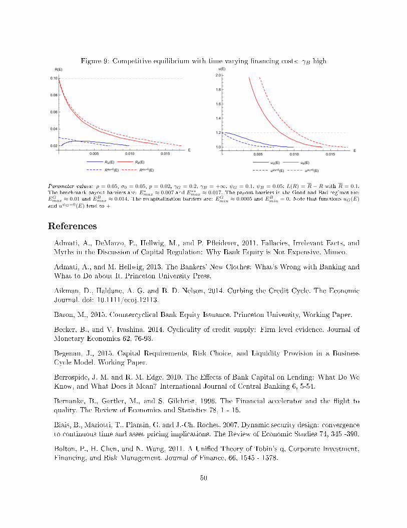
Figure 9: Competitive equilibrium with time-varying �nancing costs: γB high

0.005 0.010 0.015E

0.02

0.04

0.06

0.08

0.10

R(E)

RG(E) RB(E)

RψB=0(E) RψG=0(E)

0.005 0.010 0.015E

1.0

1.2

1.4

1.6

1.8

2.0

u(E)

uG(E) uB(E)

uψB=0(E) uψG=0(E)

Parameter values: ρ = 0.05, σ0 = 0.05, p = 0.02, γG = 0.2, γB = +∞, ψG = 0.1, ψB = 0.05; L(R) = R − R with R = 0.1.The benchmark payout barriers are: E∗max ≈ 0.007 and E∗∗max ≈ 0.017. The payout barriers in the Good and Bad regimes are:EGmax ≈ 0.01 and EBmax ≈ 0.014. The recapitalization barriers are: EGmin ≈ 0.0005 and EBmin = 0. Note that functions uG(E)

and uψG=0(E) tend to +

References

Admati, A., DeMarzo, P., Hellwig, M., and P. P�eiderer, 2011. Fallacies, Irrelevant Facts, andMyths in the Discussion of Capital Regulation: Why Bank Equity is Not Expensive. Mimeo.

Admati, A., and M. Hellwig, 2013. The Bankers' New Clothes: What's Wrong with Banking andWhat to Do about It. Princeton University Press.

Aikman, D., Haldane, A. G. and B. D. Nelson, 2014. Curbing the Credit Cycle. The EconomicJournal. doi: 10.1111/ecoj.12113.

Baron, M., 2015. Countercyclical Bank Equity Issuance. Princeton University, Working Paper.

Becker, B., and V. Ivashina, 2014. Cyclicality of credit supply: Firm level evidence. Journal ofMonetary Economics 62, 76-93.

Begenau, J., 2015. Capital Requirements, Risk Choice, and Liquidity Provision in a BusinessCycle Model. Working Paper.

Berrospide, J. M. and R. M. Edge, 2010. The E�ects of Bank Capital on Lending: What Do WeKnow, and What Does it Mean? International Journal of Central Banking 6, 5-54.

Bernanke, B., Gertler, M., and S. Gilchrist, 1996. The Financial accelerator and the �ight toquality. The Review of Economics and Statistics 78, 1 - 15.

Biais, B., Mariotti, T., Plantin, G. and J.-Ch. Rochet, 2007. Dynamic security design: convergenceto continuous time and asset pricing implications. The Review of Economic Studies 74, 345 -390.

Bolton, P., H. Chen, and N. Wang, 2011. A Uni�ed Theory of Tobin's q, Corporate Investment,Financing, and Risk Management. Journal of Finance, 66, 1545 - 1578.

50

Bolton, P., H. Chen, and N. Wang, 2013. Market Timing, Investment, and Risk Management.Journal of Financial Economics 109, 40 - 62.

Brunnermeier, M. K. and Y. Sannikov, 2014. A Macroeconomic Model with a Financial Sector.American Economic Review 104, 379 - 421.

Conrad, J., Dittmar, R.F., and A. Hameed, 2013. Cross-Market and Cross-Firm E�ects in ImpliedDefault Probabilities and Recovery Values. Working Paper.

DeAngelo, H., and R. M. Stulz, 2014. Why High Leverage is Optimal for Banks. Fisher Collegeof Business WP 2013-03-08.

Décamps, J.P., T. Mariotti, J.C. Rochet, and S. Villeneuve, 2011. Free Cash Flow, Issuance Costs,and Stock Prices. Journal of Finance, 66, 1501-1544.

Dell'Ariccia, G., and R. Marquez, 2006. Lending Booms and Lending Standards. Journal of Fi-nance 61, 2511 - 2546.

De Nicolò, G., A. Gamba, and M. Lucchetta, 2014. Microprudential Regulation in a DynamicModel of Banking. Review of Financial Studies 27, 2097 - 2138.

Diamond, D., and P. Dybvig, 1983. Bank runs, deposit insurance, and liquidity. Journal of PoliticalEconomy 99, 689-721.

Di Tella, S., 2014. Uncertainty Shocks and Balance Sheet Recessions. Working Paper, StanfordGSB.

Freixas, X. and J.-Ch. Rochet, 2008. Microeconomics of Banking, MIT Press.

Gornall, W., and I. A., Strebulaev, 2015. Financing as a Supply Chain: The Capital Structure ofBanks and Borrowers. Working Paper.

He, Z. and A. Krishnamurthy, 2012. A Model of Capital and Crises. Review of Economic Studies79, 735-77.

He, Z. and A. Krishnamurthy, 2013. Intermediary Asset Pricing. American Economic Review 103,732 - 770.

Hellwig, M., 2015. Liquidity provision and Equity Funding of Banks. Discussion Paper, MaxPlanck Institute.

Hennessy, C. A. and T. M. Whited, 2007. How costly is external �nancing: Evidence from astructural estimation. Journal of Finance 62, 1705 - 1745.

Hugonnier, J. N., and E. Morellec, 2015. Bank Capital, Liquid Reserves, and Insolvency Risk.Working Paper, Swiss Finance Institute and EPFL.

Isohätälä, J., Milne A., and D. Robertson, 2014. The net worth trap: investment and outputdynamics in the presence of �nancing constraints. Bank of Finland Research Discussion PaperNo. 26/2014.

51

Jeanblanc, M., and A. N. Shiryaev, 1995. Optimization of the �ow of dividends. Russian Mathe-matical Surveys 50, 257 - 277.

Jiménez, G., and J. Saurina, 2006. Credit Cycles, Credit Risk, and Prudential Regulation. Inter-national Journal of Central Banking 2, 65-98.

Kiyotaki, N. and J. Moore, 1997. Credit Cycles. Journal of Political Economy 105, 211 - 48.

Lee, I., S. Lochhead, J. Ritter, and Q. Zhao, 1996. The Costs of Raising Capital. Journal ofFinancial Research 19 , 59-74.

Lorenzoni,G., 2008. Ine�cient Credit Booms. Review of Economic Studies 75(3), 809 - 833.

Malherbe, F., 2015. Optimal capital requirements over the business and �nancial cycles. ECBWorking Paper 1830.

Martinez-Miera, D., and R. Repullo, 2010. Does Competition Reduce the Risk of Bank Failure?Review of Financial Studies 23, 3638 -3664.

Martinez-Miera, D., and J. Suarez, 2014. A Macroeconomic Model of Endogenous Systemic RiskTaking. Mimeo, CEMFI.

Milne, A., Robertson, D., 1996. Firm behavior under the threat of liquidation. Journal of EconomicDynamics and Control 20, 1427 - 1449.

Nguyên, T., 2014. Bank Capital Requirements: A quantitative Analysis. Working Paper.

Phelan, G., 2015. Financial Intermediation, Leverage, and Macroeconomic Instability. Forthcom-ing in American Economic Journal: Macroeconomics.

Stein, J., 2012. Monetary Policy as Financial Stability Regulation. Quarterly Journal of Economics127, 57-95.

TheCityUK report, October 2013. Alternative �nance for SMEs and mid-market companies.

Van den Heuvel, S. J., 2008. The welfare cost of bank capital requirements. Journal of MonetaryEconomics 55, 298 - 320.

52