Aggregate Bank Capital and Credit Dynamics

Nataliya Klimenko∗ Sebastian Pfeil † Jean-Charles Rochet ‡ Gianni De Nicolò §

First draft: December, 2014

This version: November, 2015

Abstract

Central banks need a new type of quantitative models for guiding their �nancial stability

decisions. The aim of this paper is to propose such a model. In our model commercial

banks �nance their loans by deposits and equity, while facing issuance costs when they raise

new equity. Because of this �nancial friction, banks build equity bu�ers to absorb negative

shocks. Aggregate bank capital determines the dynamics of credit. Notably, the equilibrium

loan rate is a decreasing function of aggregate capitalization. The competitive equilibrium is

constrained ine�cient, because banks do not internalize the e�ect of their individual lending

decisions on the future loss-absorbing capacity of the banking sector. In particular, we �nd

that undercapitalized banks lend too much. We show that introducing a minimum capital

ratio helps taming excessive lending and enhances �nancial stability.

Keywords: macro-model with a banking sector, aggregate bank capital, pecuniary externality,

capital requirements

JEL: E21, E32, F44, G21, G28

Acknowledgements: we thank George-Marios Angeletos, Manuel Arellano, Philippe Bacchetta, Bruno Biais, Markus

Brunnermeier, Catherine Casamatta, Julien Daubanes, Peter DeMarzo, Jean-Paul Décamps, Sebastian Di Tella, John Geanako-

plos, Hans Gersbach, Hendrik Hakenes, Christian Hellwig, Eric Jondeau, Simas Kucinskas, Li (Erica) Xuenan, Michael Magill,

Semyon Malamud, Loriano Mancini, David Martinez-Miera, Erwan Morellec, Alistair Milne, Henri Pagès, Bruno Parigi, Greg

Phelan, Guillaume Plantin, Martine Quinzii, Raphael Repullo, Yuliy Sannikov, Enrique Sentana, Amit Seru, Jean Tirole and

Stéphane Villeneuve, and seminar participants at CEMFI, ETH Zürich, Princeton University, Stanford University, Toulouse

School of Economics, EPF Lausanne, the University of Nanterre, Yale University and Banque de France, University of Bonn,

and the CICF 2015 conference.

∗University of Zürich. E-mail: nataliya.klimenko@bf.uzh.ch.†University of Bonn. E-mail: pfeil@uni-bonn.de.‡University of Zürich, SFI and TSE-IDEI. E-mail: jean-charles.rochet@bf.uzh.ch.§International Monetary Fund and CESifo. E-mail: GDeNicolo@imf.org.

1

1 Introduction

Central banks need quantitative models for guiding their �nancial stability decisions. Indeed,

in the context of their new macro-prudential responsibilities, they have recently been endowed

with powerful regulatory tools. These tools include the setting of capital requirements for all

banks, determining capital add-ons for systemic institutions, and deciding when to activate counter-

cyclical capital bu�ers. The problem is nobody has the slightest idea of the long term impact of

these regulations on growth and �nancial stability. The only quantitative models that central

banks currently have at their disposal, the so-called DSGE models, have been designed for very

di�erent purposes, namely assessing the short term impact of monetary policy decisions on in�ation

and economic activity. Until recently, these DSGE models did not even include banks in their

representation of the economy. DSGE models are very complex and use very special assumptions,

because they have been speci�cally calibrated to reproduce the short term reaction of prices and

employment to movements in central banks' policy rates. It seems therefore clear that a very

di�erent kind of model is needed for analyzing the long term impact of capital regulations (and

other macro-prudential tools) on bank credit, GDP growth and �nancial stability. The aim of this

paper is to propose such a model.

Building on the recent literature on macro models with �nancial frictions, we develop a tractable

dynamic model where aggregate bank capital determines the dynamics of credit. Though highly

stylized, the model is able to generate predictions in line with empirical evidence. We consider an

economy where �rms borrow from banks that are �nanced by deposits and equity. The aggregate

supply of bank loans is confronted with the �rms' demand for credit, which determines the equilib-

rium loan rate. Aggregate shocks impact the �rms' default probability, which ultimately translates

into pro�ts or losses for banks. Banks can continuously adjust their volumes of lending to �rms.

They also decide when to distribute dividends and when to issue new equity. Equity issuance is

subject to deadweight costs, which constitutes the main �nancial friction in our economy and creates

room for the loss-absorbing role of bank capital.1

In a set-up without �nancial frictions (i.e., no issuance costs for bank equity) and i.i.d. ag-

gregate shocks, the equilibrium volume of lending and the nominal loan rate would be constant.

Furthermore, dividend payment and equity issuance policies would be trivial in this case: Banks

would immediately distribute all pro�ts as dividends and would issue new shares to o�set losses and

honor obligations to depositors. This implies that, in a frictionless world, there would be no need

to build up capital bu�ers and all loans would be entirely �nanced by deposits.

When �nancial frictions are taken into account, banks' dividend and equity issuance strategies

become less trivial. We show that there is a unique competitive equilibrium, where all variables of

1Empirical studies report sizable costs of seasoned equity o�erings (see e.g. Lee, Lochhead, Ritter, and Zhao(1996), Hennessy and Whited (2007)). Here we follow the literature (see e.g. Décamps et al. (2011) or Bolton et al.(2011)) by assuming that issuing new equity entails a deadweight cost proportional to the size of the issuance.

interest are deterministic functions of the total book value of bank equity, which follows a Markov

process re�ected at two boundaries. Banks issue new shares at the lower boundary, where total book

equity of the banking sector is depleted. When total bank equity reaches its upper boundary, any

further earnings are paid out to shareholders as dividends. Between these boundaries, the changes

in banks' equity are only due to their pro�ts and losses. Banks retain earnings in order to increase

their loss-absorbing equity bu�er and thereby reduce the frequency of costly recapitalizations. This

bu�er is needed to guarantee the safety of deposits.2

We start by exploring the properties of the competitive equilibrium in the �laissez-faire� environ-

ment, in which banks face no regulation. We �rst set up the model in discrete time to provide the

main economic intuitions. We then present a continuous time version that leads to quasi explicit

solutions. This turns out to be helpful for illustrating the features of the equilibrium, notably the

long run dynamics. Even though all agents are risk neutral, our model generates a positive spread

for bank loans. This spread is decreasing in the level of total bank equity. To get an intuition for

this result, note that bank equity is more valuable when it is scarce because pro�t margins are a

decreasing function of total bank equity. Therefore, the marginal (or market-to-book) value of eq-

uity is higher when total bank equity is lower. Moreover, pro�ts and losses are positively correlated

across banks. Thus each bank anticipates that total bank equity will be lower (higher) in the states

of the world where it makes losses (pro�ts). Individual losses are thus ampli�ed by a simultaneous

increase in the market-to-book value, whereas individual pro�ts are moderated by a simultaneous

decrease in the market-to-book value. As a result, banks only lend to �rms when the loan rate

incorporates an appropriate premium.

In the continuous-time set-up, the equilibrium dynamics of the loan rate can be obtained in

closed form, which enables us to study the long-run behavior of the economy by looking at the

properties of the ergodic density function of total bank equity. Our analysis shows that the long-

run behavior of the economy is mainly driven by the (endogenous) volatility of total bank equity. In

particular, the economy spends most of the time in states with low endogenous volatility. For high

recapitalization costs and a low elasticity of demand for bank loans, this can induce long periods of

persistently low volumes of credit and low levels of bank equity.

We show that the competitive equilibrium is constrained ine�cient. The reason is that com-

petitive banks do not internalize the impact of their individual lending decisions on i) the banking

system's exposure to aggregate shocks and ii) the pro�t margin on credit. As a result, banks typ-

ically lend too much as compared to the socially optimal level, creating ine�ciently high exposure

to macroeconomic shocks when the banking system is poorly capitalized. Furthermore, ine�ciently

low pro�t margins undermine the banking system's ability to accumulate loss absorbing capital

2The idea that bank equity is needed to guarantee the safety of deposits is explored in several recent papers. Stein(2012) shows its implication for the design of monetary policy. Hellwig (2015) develops a static general equilibriummodel where bank equity is necessary to support the provision of safe and liquid investments to consumers. DeAngeloand Stulz (2014) and Gornall and Strebulaev (2015) argue that, due to the banks' ability to diversify risk, the actualsize of this equity bu�er may be very small.

2

through retained earnings.

We use our model to explore the impact of bank capital requirements. A standard argument

against high capital requirements is that they would reduce lending and growth. By contrast,

the proponents of higher capital requirements put emphasis on their positive impact on �nancial

stability. Solving for the competitive equilibrium under imposed minimum capital requirements

enables us to consider the interplay between the aforementioned e�ects and get some insight into

the long run consequences of a substantial increase in minimum capital requirements.

In our framework, imposing a higher capital ratio indeed translates into a higher loan rate and

thus reduces lending for any given level of bank capitalization. Importantly, this e�ect is present even

when the regulatory constraint is not binding, because banks anticipate that capital requirements

might be binding in the future and require a higher lending premium for precautionary motives.

However, reduction in lending also reduces the banks' exposure to aggregate shocks, while higher

loan rates fosters a quicker accumulation of earnings and thus allows for a quicker recovery after

the negative shocks, which ultimately makes the banking sector more stable. As a result, in the

long run, the economy spends more time in the states of the world with abundant bank capital and

cheap credit.

Related literature. From a technical perspective, our paper follows the approach of the new gener-

ation of the continuous-time macroeconomic models with �nancial frictions (see e.g. Brunnermeier

and Sannikov (2014, 2015), Di Tella (2015), He and Krishnamurthy (2012, 2013)). Seeking for a

better understanding of the transmission mechanisms of monetary policy and the consequences of

�nancial instability, all these papers point out to the key role that balance-sheet constraints and

net-worth of �nancial intermediaries may play in (de)stabilizing the economy in the presence of

�nancing frictions and aggregate shocks. We extend this literature by modeling the banking sector

explicitly and relating total bank equity to credit dynamics and �nancial stability. A closely related

paper is Phelan (2015) who explicitly introduces a banking sector in a continuous-time general

equilibrium model. In Phelan's paper also, banks invest in productive capital (land) and depositors

obtain utility from holding safe deposits. The focus of our analysis is di�erent: we explicitly study

the impact of bank capitalization on the dynamics of the loan rate.

A common feature of the above-mentioned papers is the existence of �re-sale externalities in the

spirit of Kiyotaki and Moore (1997) and Lorenzoni (2008) that arise when forced asset sales depress

prices, which in turn creates amplifying feedback e�ects. In our model, ampli�cation and persistent

investment distortions emerge even in the absence of �re sales. The main externality imposed by

individual banks' lending decisions is that each bank fails to internalize the impact of its lending

choice on the banking system's exposure to aggregate risk, which increases endogenous volatility.

Furthermore, the idea that �erce competition can have a destabilizing e�ect as it erodes banks'

pro�t margins and, thus, their ability to accumulate loss absorbing capital is related to Martinez-

Miera and Repullo (2010). A similar externality is present in the overlapping generations model

3

considered by Malherbe (2015): Individual banks neglect the fact that an expansion of lending,

due to diminishing returns to productive capital, leads to a deterioration of the marginal loan and,

thus, higher bankruptcy costs for all banks in the economy. As a result, banks lend in excessively

in booms, which calls for counter-cyclical capital requirements.

The extended version of our model featuring the regulatory leverage constraint contributes to the

ongoing investigations of the welfare e�ects of capital regulation. Most of the literature dealing with

this issue is focused on the trade-o� between the welfare gains from the mitigation of risk-taking

incentives on the one hand3 and welfare losses caused by lower liquidity provision (e.g., Begenau

(2015), Van den Heuvel (2008)), lower lending and output (e.g., Nguyên (2014), Martinez-Miera

and Suarez (2014)) on the other hand.4 In contrast to the above-mentioned studies, the focus of our

model is entirely shifted from the incentive e�ect of bank capital towards its role of a loss absorbing

bu�er - the concept that is often put forward by bank regulators. Moreover, the main contribution

of our paper is qualitative: we seek to identify the long run e�ects of capital regulation rather than

provide a quantitative guidance on the optimal level of a minimum capital ratio.

More broadly, this paper relates to the literature on credit cycles that has brought forward a

number of alternative explanations for their occurrence. Fisher (1933) identi�ed the famous debt

de�ation mechanism, that has been further formalized by Bernanke et al. (1996) and Kiyotaki

and Moore (1997). It attributes the origin of credit cycles to the �uctuations of the prices of

collateral. Several studies also place emphasis on the role of �nancial intermediaries, by pointing

out the fact that credit expansion is often accompanied by a loosening of lending standards and

"systemic" risk-taking, whereas materialization of risk accumulated on the balance sheets of �nancial

intermediaries leads to the contraction of credit (see e.g. Aikman et al. (2014), Dell'Ariccia and

Marquez (2006), Jimenez and Saurina (2006)). In our model, quasi cyclical lending patterns emerge

due to the re�ection property of aggregate bank capital that follows from the optimality of �barrier�

recapitalization and dividend strategies.

The rest of the paper is organized as follows. Section 2 presents a simple one-period model that

conveys the main intuitions concerning the economic forces working in the full-�edged dynamic set-

up. In Section 3 we characterize the competitive equilibrium in the discrete-time in�nite-horizon

dynamic set-up. Section 4 presents the continuous-time version of the model, illustrating its ap-

plication for studying the long-run macrodynamics and discussing ine�ciencies inherent in the

competitive equilibrium framework. In Section 5 we introduce capital regulation, analysing its im-

plications for bank policies and the lending-stability trade-o�. Section 6 concludes. All proofs,

model extensions and computational details are gathered in Appendices A-F. Appendix G reports

3Bank capital is often viewed as �skin in the game� needed to prevent the opportunistic behaviours of banks'insiders.

4The only exception is the work by De Nicolò et al. (2014) that conducts the analysis of bank risk choices undercapital and liquidity regulation in a fully dynamic model, where capital plays the role of a shock absorber, anddividends, retained earnings and equity issuance are modeled under a �nancial friction captured by a constraint oncollateralized debt.

4

the results of the empirical analysis supporting the key model predictions.

2 One-period model

Before setting-up the fully �edged dynamic model, it is useful to convey some key intuitions in a

static benchmark. We start by describing the intermediation and production technologies and then

characterize the competitive equilibrium.

2.1 The model set-up

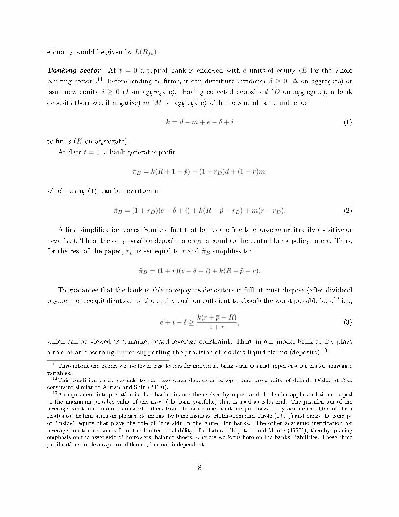
The static model has only two dates t = 0 and t = 1. There is one physical good, taken as a

numeraire, which can be consumed at t = 0 or invested to produce consumption at t = 1. Banks

are needed to channel savings of households to the productive sector.5 Savings take two possible

forms: riskless deposits and risky equity. Banks' assets consist of loans to the productive sector

(see Figure 1) and reserves at the central banks. Banks are competitive: they take both the deposit

interest rate rD ≥ 0 and loan rate R as given. The central bank sets the rate r at which banks can

deposit reserves or re�nance. Households cannot directly invest in the productive sector. Instead, at

t = 0, they invest in deposit and equity claims issued by banks, who then grant loans to �rms. Firms

are run by penniless entrepreneurs that immediately consume all output net of the loan repayments

to banks. Thus, the entire volume of productive investment in the economy is determined by the

volume of bank credit.6 Apart from channelling funding to the productive sector, the major reason

why banks matter in our framework is that bank capital allows to bu�er losses on loans. As will

be shown further, only the aggregate loss absorbing capacity of the banking sector matters for our

analysis, whereas the number of banks and their individual sizes do not play any role.

The main �nancial friction in our model is that issuing new bank equity entails a proportional

cost γ.

Preferences. Households have identical quasi-linear preferences with a discount rate ρ. At t = 0

they receive an endowment w0 of the good that they allocate between consumption C0, deposits D

and investment I in bank equity:

w0 = C0 +D + (1 + γ)I.

Following Stein (2012), we assume that households derive utility both from consumption and

from payment services provided by bank deposits, as long as banks can guarantee perfect safety of

5This standard assumption is usually justi�ed by technological and informational reasons (see e.g. Freixas andRochet(2008), Chapter 2).

6In our model, �rms should be thought of as small and medium-sized enterprises (SMEs), which typically rely onbank �nancing. As is well known, the importance of bank �nancing varies across countries. For example, accordingto the TheCityUK research report (October 2013), in EU area, bank loans account for 81% of the long term debt inthe real sector, whereas in the U.S. the same ratio amounts to 19%.

5

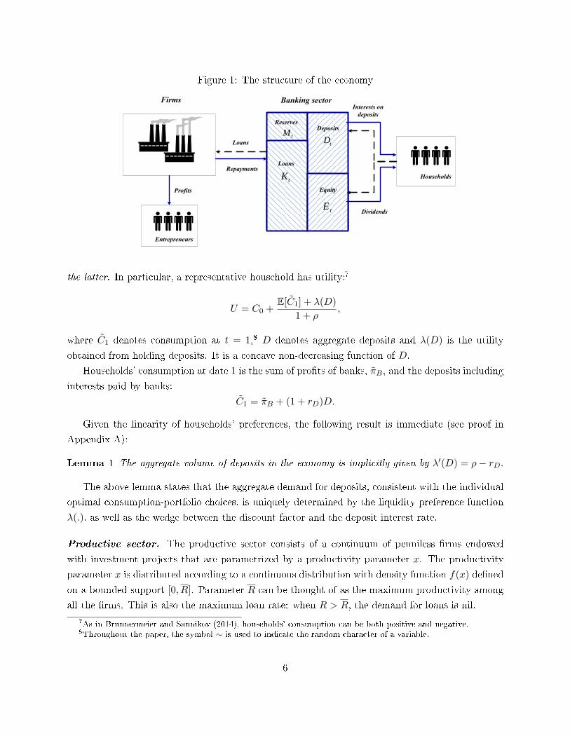
Figure 1: The structure of the economy

tKLoans

tE

Deposits

Equity

Banking sector

Loans

Repayments

Households

Profits

tD

Interests on

deposits

Dividends

Firms

Reserves

tM

Entrepreneurs

the latter. In particular, a representative household has utility:7

U = C0 +E[C1] + λ(D)

1 + ρ,

where C1 denotes consumption at t = 1,8 D denotes aggregate deposits and λ(D) is the utility

obtained from holding deposits. It is a concave non-decreasing function of D.

Households' consumption at date 1 is the sum of pro�ts of banks, πB, and the deposits including

interests paid by banks:

C1 = πB + (1 + rD)D.

Given the linearity of households' preferences, the following result is immediate (see proof in

Appendix A):

Lemma 1 The aggregate volume of deposits in the economy is implicitly given by λ′(D) = ρ− rD.

The above lemma states that the aggregate demand for deposits, consistent with the individual

optimal consumption-portfolio choices, is uniquely determined by the liquidity preference function

λ(.), as well as the wedge between the discount factor and the deposit interest rate.

Productive sector. The productive sector consists of a continuum of penniless �rms endowed

with investment projects that are parametrized by a productivity parameter x. The productivity

parameter x is distributed according to a continuous distribution with density function f(x) de�ned

on a bounded support [0, R]. Parameter R can be thought of as the maximum productivity among

all the �rms. This is also the maximum loan rate: when R > R, the demand for loans is nil.

7As in Brunnermeier and Sannikov (2014), households' consumption can be both positive and negative.8Throughout the paper, the symbol ∼ is used to indicate the random character of a variable.

6

Firms' projects require each an investment of one unit of good at t = 0. A typical project

yields x units of good at t = 1 with certainty. For the sake of simplicity, we assume that the �rm

always repays the interest R on the loan. However, with some probability, productive capital can

be destroyed and the bank only gets R, whereas the �rm always gets (x−R). Firms are protected

by limited liability and default when their projects are not successful. Given a nominal loan rate R,

only the projects such that x > R will demand �nancing. Thus, the total demand for bank loans

in the economy is:

L(R) =

∫ R

Rf(x)dx.

We focus on the simple case where all projects have the same default probability p that depends

on the realization of aggregate shocks. For simplicity, we assume that it can take only two values:9

p =

p, with probability 1− q (positive shock) ,

p, with probability q (negative shock),

where 1 > p > p > 0.

Therefore, the net return per loan for a bank at date t = 1 is

R− rD − p,

and the net aggregate output per period in the economy is

F [L(R)]− pL(R),

where F [L(R)] is the aggregate production function:

F [L(R)] =

∫ R

Rxf(x)dx.

Note that F ′[L(R)] ≡ R,10 so that the total expected surplus per unit of time

F [L(R)]− L(R)(rD + E[p]

)is maximized for Rfb = rD + E[p]. Thus, in the �rst best allocation, the loan rate is the sum of

two components: the riskless rate and the expected probability of default. This implies that, in the

�rst-best allocation, banks would make zero expected pro�t, and the total volume of credit in the

9The extension to heterogeneous default probability is straightforward and would not change our qualitativeresults.

10Di�erentiating F [L(R)] =∫ RRxf(x)dx with respect to R yields F ′[L(R)]L′(R) = −Rf(R). Since L′(R) = −f(R),

this implies F ′[L(R)] ≡ R.

7

economy would be given by L(Rfb).

Banking sector. At t = 0 a typical bank is endowed with e units of equity (E for the whole

banking sector).11 Before lending to �rms, it can distribute dividends δ ≥ 0 (∆ on aggregate) or

issue new equity i ≥ 0 (I on aggregate). Having collected deposits d (D on aggregate), a bank

deposits (borrows, if negative) m (M on aggregate) with the central bank and lends

k = d−m+ e− δ + i (1)

to �rms (K on aggregate).

At date t = 1, a bank generates pro�t

πB = k(R+ 1− p)− (1 + rD)d+ (1 + r)m,

which, using (1), can be rewritten as

πB = (1 + rD)(e− δ + i) + k(R− p− rD) +m(r − rD). (2)

A �rst simpli�cation cones from the fact that banks are free to choose m arbitrarily (positive or

negative). Thus, the only possible deposit rate rD is equal to the central bank policy rate r. Thus,

for the rest of the paper, rD is set equal to r and πB simpli�es to:

πB = (1 + r)(e− δ + i) + k(R− p− r).

To guarantee that the bank is able to repay its depositors in full, it must dispose (after dividend

payment or recapitalization) of the equity cushion su�cient to absorb the worst possible loss,12 i.e.,

e+ i− δ ≥ k(r + p−R)

1 + r, (3)

which can be viewed as a market-based leverage constraint. Thus, in our model bank equity plays

a role of an absorbing bu�er supporting the provision of riskless liquid claims (deposits).13

11Throughout the paper, we use lower case letters for individual bank variables and upper case letters for aggregatevariables.

12This condition easily extends to the case when depositors accept some probability of default (Value-at-Riskconstraint similar to Adrian and Shin (2010)).

13An equivalent interpretation is that banks �nance themselves by repos, and the lender applies a hair cut equalto the maximum possible value of the asset (the loan portfolio) that is used as collateral. The justi�cation of theleverage constraint in our framework di�ers from the other ones that are put forward by academics. One of themrelates to the limitation on pledgeable income by bank insiders (Holmstrom and Tirole (1997)) and backs the conceptof "inside" equity that plays the role of "the skin in the game" for banks. The other academic justi�cation forleverage constraints stems from the limited resalability of collateral (Kiyotaki and Moore (1997)), thereby, placingemphasis on the asset side of borrowers' balance sheets, whereas we focus here on the banks' liabilities. These threejusti�cations for leverage are di�erent, but not independent.

8

2.2 Competitive equilibrium in the one-period model

Our objective now is to solve for the competitive equilibrium in this static framework. The

competitive equilibrium is characterized by a loan rate R, a lending volumeK and aggregate reserves

M that are compatible with the equilibrium conditions on credit, equity and deposit markets, as

well as pro�t maximization by individual banks.

Consider �rst the maximization problem of a typical bank. Each bank takes the loan rate R as

given and chooses dividend policy δ ≥ 0, recapitalization policy i ≥ 0 and the volume of lending

k ≥ 0 so as to maximize shareholder value, while insuring compliance with the market-based leverage

constraint:

v = maxδ≥0,i≥0,k>0

{δ − (1 + γ)i+

(1− q)πB(p) + qπB(p)

1 + ρ+θπB(p)

1 + ρ

},

where πB(p) is the pro�t realization under the positive aggregate shock, πB(p) is the pro�t realization

after the negative aggregate shock and θ denotes the Lagrange multiplier associated with the market-

based leverage constraint.

Note that the above maximization problem is separable, i.e.,

v = e(1 + r)(1 + θ)

1 + ρ+ max

δ≥0δ[1− (1 + r)(1 + θ)

1 + ρ

]+ max

i≥0i[− (1 + γ) +

(1 + r)(1 + θ)

1 + ρ

]+ max

k>0k[R− E[p]− r − θ(r + p−R)

1 + ρ

].

(4)

Optimizing with respect to the bank's policies yields the following conditions:

1− (1 + r)(1 + θ)

1 + ρ≤ 0 (= if δ > 0), (5)

− (1 + γ) +(1 + r)(1 + θ)

1 + ρ≤ 0 (= if i > 0), (6)

R− E[p]− r = θ(r + p−R). (7)

Condition (5) shows that θ > 0, which implies that the market-based leverage constraint is

always binding at both the individual and aggregate levels. This determines completely the loan

rate as a function of aggregate bank capitalization, i.e., R ≡ R(E). More speci�cally, when δ = 0

and i = 0, loan rate R ≡ R(E) is the unique solution of the equation:

L(R)(R− p− r) + (1 + r)E = 0.

Equation (7) then determines the value of θ, which also depends on E. Finally, the shareholder

9

value of each bank is proportional to its book equity, namely:

v ≡ v(e, E) = e(1 + r)(1 + θ(E))

1 + ρ= e

(1 + r)(p− E[p])

(1 + ρ)[r + p−R(E)]≡ eu(E),

where u(E) can be interpreted as the market-to-book ratio of equity. Note that u(E) is a decreasing

function of E: bank capital becomes more valuable when it is getting scarce.

It is easy to see from conditions (5) and (6), that the optimal dividend and recapitalization

policies are driven by the market-to-book ratio of bank equity. In particular, condition (5) transforms

to

u(E) ≥ 1,

and condition (6) can be rewritten as

u(E) ≤ 1 + γ.

Let Emin denote the unique level of aggregate equity such that u(Emin) = 1+γ and Emax be such

that u(Emax) = 1. Then, when E < Emin, banks will recapitalize by raising in aggregate Emin−E.Similarly, when E > Emax, aggregate dividends E − Emax are distributed to shareholders. As a

result, the market-to-book ratio of the banking sector always remains within the range [1, 1 + γ].

As will be shown further, this feature is preserved in both the discrete-time and continuous-time

dynamic versions of our model. The following proposition summarizes our results for the static

set-up:

Proposition 1 The static model has a unique competitive equilibrium. It has the following proper-

ties:

a) The loan rate R ≡ R(E) is a decreasing function of aggregate capital E and is implicitly given

by

L[R(E)][r + p−R(E)] = E(1 + r).

b) All the banks have the same market-to-book ratio of equity that is a decreasing function of E:

u(E) =(1 + r)(p− E[p])

(1 + ρ)(r + p−R(E)).

c) Banks pay dividends when E ≥ Emax ≡ u−1(1) and recapitalize when E ≤ Emin ≡ u−1(1 + γ).

d) The leverage constraint is always binding for all the banks:

k

e=L[R(E)]

E=

1 + r

r + p−R(E).

Our parsimonious static set up emphasizes the important idea that the equilibrium loan rate

10

R(E) is driven by aggregate bank capitalization E. Namely, the loan rate is lower when the banking

sector is better capitalized. Another key testable prediction generated by this simplest form of our

theoretical model is that the banks' market-to-book ratio of equity should be a decreasing function

of aggregate bank capital. Before developing the dynamic version of our theoretical model, it is

useful to examine whether these predictions are rejected by the data or not.

In Appendix G, we conduct statistical tests on a data set covering a large panel of publicly traded

banks in 43 advanced and emerging market economies for the period 1982-2013. We �nd that our

predictions �t the data extremely well. Table 3 in Appendix G shows the results of simple regressions

of loan rates and market-to-book ratios of banks equity in three sub-panels: U.S. banks, Advanced

countries' (excluding U.S.) banks and Emerging countries' banks. In all cases, the coe�cients of

Total Bank Equity are negative with p-values indistinguishable from zero.

3 Discrete-time model with in�nite horizon

We now turn to a stationary version of the static model, which has an in�nite number of periods,

t = 0, ...,∞. Our objective is to characterize Markovian competitive equilibria, where all aggregate

variables are deterministic functions of a single state variable, namely, aggregate bank equity Et.

For the sake of tractability, for the rest of the paper we assume that r = 0. The case r > 0 is

studied in Appendix D in the continuous-time framework.

De�nition 1 A (stationary) Markovian competitive equilibrium consists of an aggregate bank capi-

tal process Et, loan rate R(E) and credit volume K(E) functions that are compatible with individual

banks' pro�t maximization and the credit market clearing condition K(E) = L[R(E)].

Given the volume of lending kt, book equity of any individual bank evolves according to

et+1 − et = kt(Rt − pt)− δt + it, (8)

where δt ≥ 0 and it ≥ 0 are, respectively, individual dividend payments and recapitalizations at

date t. Similarly, aggregate capitalization of the banking sector evolves according to

Et+1 − Et = L(Rt)(Rt − pt)−∆t + It, (9)

where ∆t ≥ 0 and It ≥ 0 are, respectively, aggregate dividend payments and recapitalizations at

date t.

3.1 Markovian competitive equilibrium

To characterize the competitive equilibrium, one needs to determine the optimal recapitalization

and �nancing decisions of individual banks as well as the functional relation between the aggregate

11

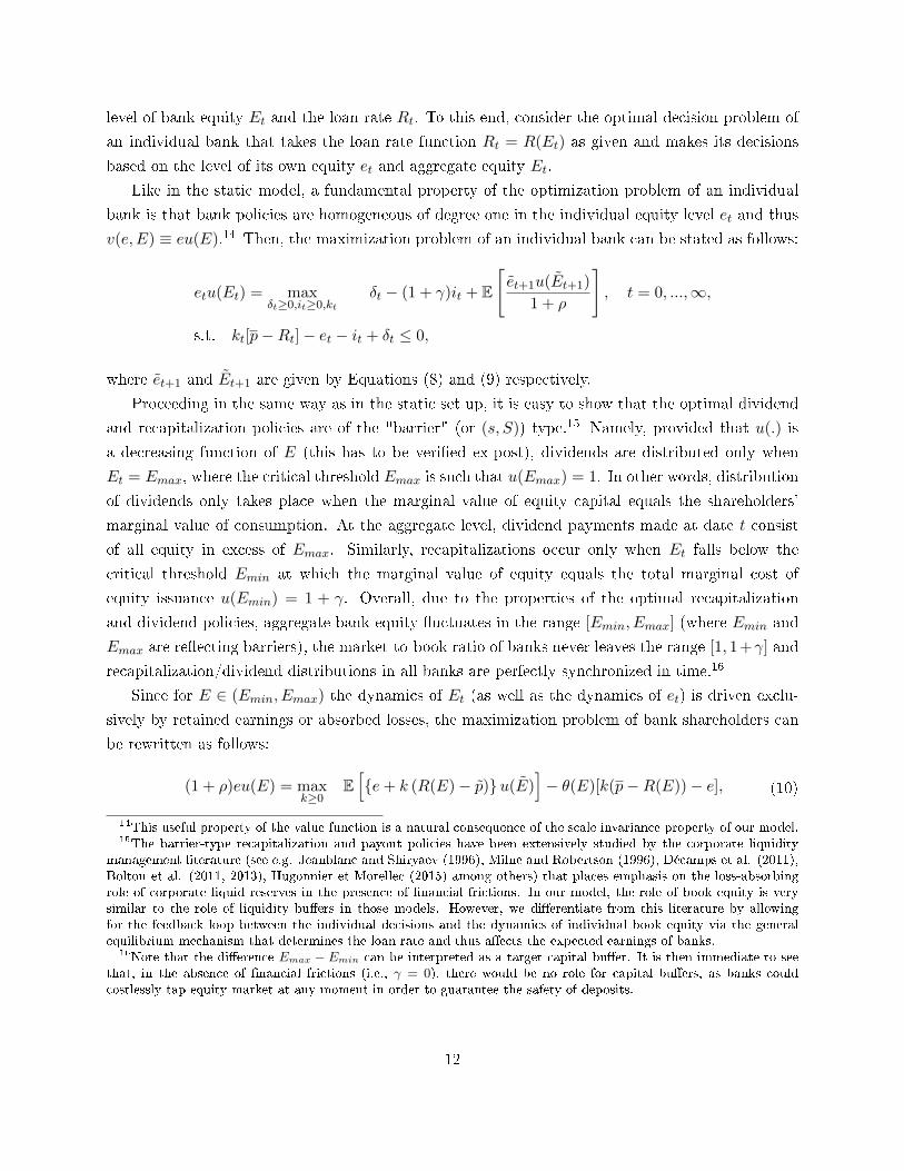
level of bank equity Et and the loan rate Rt. To this end, consider the optimal decision problem of

an individual bank that takes the loan rate function Rt = R(Et) as given and makes its decisions

based on the level of its own equity et and aggregate equity Et.

Like in the static model, a fundamental property of the optimization problem of an individual

bank is that bank policies are homogeneous of degree one in the individual equity level et and thus

v(e, E) ≡ eu(E).14 Then, the maximization problem of an individual bank can be stated as follows:

etu(Et) = maxδt≥0,it≥0,kt

δt − (1 + γ)it + E

[et+1u(Et+1)

1 + ρ

], t = 0, ...,∞,

s.t. kt[p−Rt]− et − it + δt ≤ 0,

where et+1 and Et+1 are given by Equations (8) and (9) respectively.

Proceeding in the same way as in the static set up, it is easy to show that the optimal dividend

and recapitalization policies are of the "barrier" (or (s, S)) type.15 Namely, provided that u(.) is

a decreasing function of E (this has to be veri�ed ex-post), dividends are distributed only when

Et = Emax, where the critical threshold Emax is such that u(Emax) = 1. In other words, distribution

of dividends only takes place when the marginal value of equity capital equals the shareholders'

marginal value of consumption. At the aggregate level, dividend payments made at date t consist

of all equity in excess of Emax. Similarly, recapitalizations occur only when Et falls below the

critical threshold Emin at which the marginal value of equity equals the total marginal cost of

equity issuance u(Emin) = 1 + γ. Overall, due to the properties of the optimal recapitalization

and dividend policies, aggregate bank equity �uctuates in the range [Emin, Emax] (where Emin and

Emax are re�ecting barriers), the market-to-book ratio of banks never leaves the range [1, 1+γ] and

recapitalization/dividend distributions in all banks are perfectly synchronized in time.16

Since for E ∈ (Emin, Emax) the dynamics of Et (as well as the dynamics of et) is driven exclu-

sively by retained earnings or absorbed losses, the maximization problem of bank shareholders can

be rewritten as follows:

(1 + ρ)eu(E) = maxk≥0

E[{e+ k (R(E)− p)}u(E)

]− θ(E)[k(p−R(E))− e], (10)

14This useful property of the value function is a natural consequence of the scale invariance property of our model.15The barrier-type recapitalization and payout policies have been extensively studied by the corporate liquidity

management literature (see e.g. Jeanblanc and Shiryaev (1996), Milne and Robertson (1996), Décamps et al. (2011),Bolton et al. (2011, 2013), Hugonnier et Morellec (2015) among others) that places emphasis on the loss-absorbingrole of corporate liquid reserves in the presence of �nancial frictions. In our model, the role of book equity is verysimilar to the role of liquidity bu�ers in those models. However, we di�erentiate from this literature by allowingfor the feedback loop between the individual decisions and the dynamics of individual book equity via the generalequilibrium mechanism that determines the loan rate and thus a�ects the expected earnings of banks.

16Note that the di�erence Emax − Emin can be interpreted as a target capital bu�er. It is then immediate to seethat, in the absence of �nancial frictions (i.e., γ = 0), there would be no role for capital bu�ers, as banks couldcostlessly tap equity market at any moment in order to guarantee the safety of deposits.

12

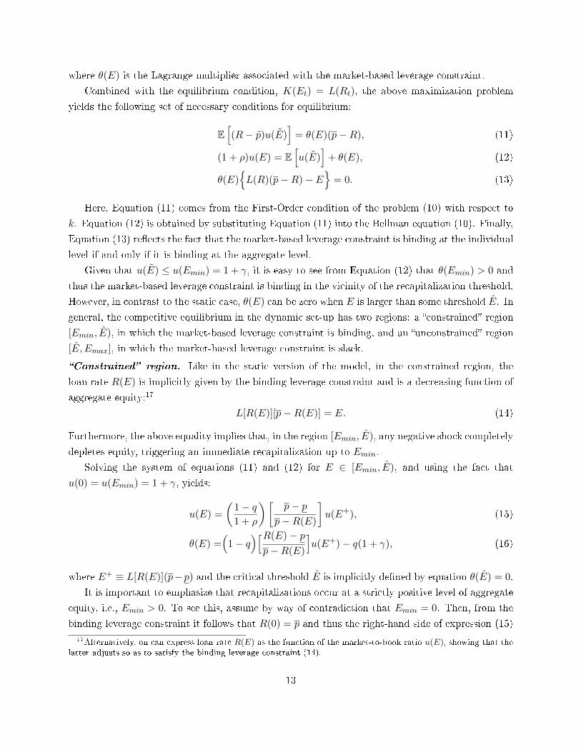
where θ(E) is the Lagrange multiplier associated with the market-based leverage constraint.

Combined with the equilibrium condition, K(Et) = L(Rt), the above maximization problem

yields the following set of necessary conditions for equilibrium:

E[(R− p)u(E)

]= θ(E)(p−R), (11)

(1 + ρ)u(E) = E[u(E)

]+ θ(E), (12)

θ(E){L(R)(p−R)− E

}= 0. (13)

Here, Equation (11) comes from the First-Order condition of the problem (10) with respect to

k. Equation (12) is obtained by substituting Equation (11) into the Bellman equation (10). Finally,

Equation (13) re�ects the fact that the market-based leverage constraint is binding at the individual

level if and only if it is binding at the aggregate level.

Given that u(E) ≤ u(Emin) = 1 + γ, it is easy to see from Equation (12) that θ(Emin) > 0 and

thus the market-based leverage constraint is binding in the vicinity of the recapitalization threshold.

However, in contrast to the static case, θ(E) can be zero when E is larger than some threshold E. In

general, the competitive equilibrium in the dynamic set-up has two regions: a �constrained� region

[Emin, E), in which the market-based leverage constraint is binding, and an �unconstrained� region

[E, Emax], in which the market-based leverage constraint is slack.

�Constrained� region. Like in the static version of the model, in the constrained region, the

loan rate R(E) is implicitly given by the binding leverage constraint and is a decreasing function of

aggregate equity:17

L[R(E)][p−R(E)] = E. (14)

Furthermore, the above equality implies that, in the region [Emin, E), any negative shock completely

depletes equity, triggering an immediate recapitalization up to Emin.

Solving the system of equations (11) and (12) for E ∈ [Emin, E), and using the fact that

u(0) = u(Emin) = 1 + γ, yields:

u(E) =

(1− q1 + ρ

)[p− p

p−R(E)

]u(E+), (15)

θ(E) =(

1− q)[R(E)− pp−R(E)

]u(E+)− q(1 + γ), (16)

where E+ ≡ L[R(E)](p−p) and the critical threshold E is implicitly de�ned by equation θ(E) = 0.

It is important to emphasize that recapitalizations occur at a strictly positive level of aggregate

equity, i.e., Emin > 0. To see this, assume by way of contradiction that Emin = 0. Then, from the

binding leverage constraint it follows that R(0) = p and thus the right-hand side of expression (15)

17Alternatively, on can express loan rate R(E) as the function of the market-to-book ratio u(E), showing that thelatter adjusts so as to satisfy the binding leverage constraint (14).

13

goes to in�nity. Yet, this contradicts the condition u(Emin) = 1 + γ that is implied by the optimal

recapitalization policy. Thus one must have Emin > 0.

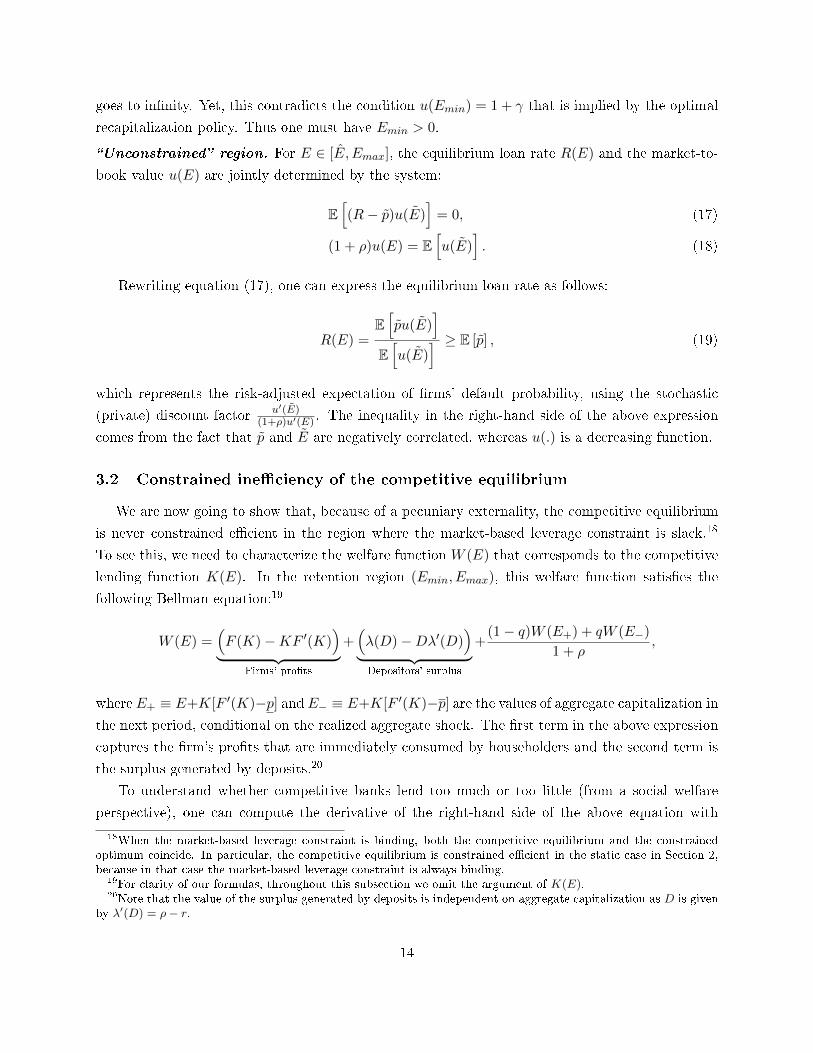
�Unconstrained� region. For E ∈ [E, Emax], the equilibrium loan rate R(E) and the market-to-

book value u(E) are jointly determined by the system:

E[(R− p)u(E)

]= 0, (17)

(1 + ρ)u(E) = E[u(E)

]. (18)

Rewriting equation (17), one can express the equilibrium loan rate as follows:

R(E) =E[pu(E)

]E[u(E)

] ≥ E [p] , (19)

which represents the risk-adjusted expectation of �rms' default probability, using the stochastic

(private) discount factor u′(E)(1+ρ)u′(E) . The inequality in the right-hand side of the above expression

comes from the fact that p and E are negatively correlated, whereas u(.) is a decreasing function.

3.2 Constrained ine�ciency of the competitive equilibrium

We are now going to show that, because of a pecuniary externality, the competitive equilibrium

is never constrained e�cient in the region where the market-based leverage constraint is slack.18

To see this, we need to characterize the welfare function W (E) that corresponds to the competitive

lending function K(E). In the retention region (Emin, Emax), this welfare function satis�es the

following Bellman equation:19

W (E) =(F (K)−KF ′(K)

)︸ ︷︷ ︸

Firms' pro�ts

+(λ(D)−Dλ′(D)

)︸ ︷︷ ︸Depositors' surplus

+(1− q)W (E+) + qW (E−)

1 + ρ,

whereE+ ≡ E+K[F ′(K)−p] andE− ≡ E+K[F ′(K)−p] are the values of aggregate capitalization inthe next period, conditional on the realized aggregate shock. The �rst term in the above expression

captures the �rm's pro�ts that are immediately consumed by householders and the second term is

the surplus generated by deposits.20

To understand whether competitive banks lend too much or too little (from a social welfare

perspective), one can compute the derivative of the right-hand side of the above equation with

18When the market-based leverage constraint is binding, both the competitive equilibrium and the constrainedoptimum coincide. In particular, the competitive equilibrium is constrained e�cient in the static case in Section 2,because in that case the market-based leverage constraint is always binding.

19For clarity of our formulas, throughout this subsection we omit the argument of K(E).20Note that the value of the surplus generated by deposits is independent on aggregate capitalization as D is given

by λ′(D) = ρ− r.

14

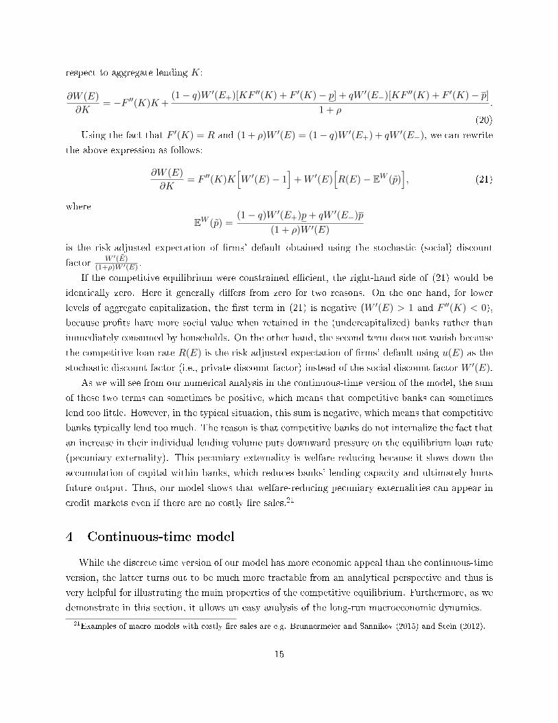
respect to aggregate lending K:

∂W (E)

∂K= −F ′′(K)K+

(1− q)W ′(E+)[KF ′′(K) + F ′(K)− p] + qW ′(E−)[KF ′′(K) + F ′(K)− p]1 + ρ

.

(20)

Using the fact that F ′(K) = R and (1 + ρ)W ′(E) = (1− q)W ′(E+) + qW ′(E−), we can rewrite

the above expression as follows:

∂W (E)

∂K= F ′′(K)K

[W ′(E)− 1

]+W ′(E)

[R(E)− EW (p)

], (21)

where

EW (p) =(1− q)W ′(E+)p+ qW ′(E−)p

(1 + ρ)W ′(E)

is the risk-adjusted expectation of �rms' default obtained using the stochastic (social) discount

factor W ′(E)(1+ρ)W ′(E) .

If the competitive equilibrium were constrained e�cient, the right-hand side of (21) would be

identically zero. Here it generally di�ers from zero for two reasons. On the one hand, for lower

levels of aggregate capitalization, the �rst term in (21) is negative (W ′(E) > 1 and F ′′(K) < 0),

because pro�ts have more social value when retained in the (undercapitalized) banks rather than

immediately consumed by households. On the other hand, the second term does not vanish because

the competitive loan rate R(E) is the risk-adjusted expectation of �rms' default using u(E) as the

stochastic discount factor (i.e., private discount factor) instead of the social discount factor W ′(E).

As we will see from our numerical analysis in the continuous-time version of the model, the sum

of these two terms can sometimes be positive, which means that competitive banks can sometimes

lend too little. However, in the typical situation, this sum is negative, which means that competitive

banks typically lend too much. The reason is that competitive banks do not internalize the fact that

an increase in their individual lending volume puts downward pressure on the equilibrium loan rate

(pecuniary externality). This pecuniary externality is welfare reducing because it slows down the

accumulation of capital within banks, which reduces banks' lending capacity and ultimately hurts

future output. Thus, our model shows that welfare-reducing pecuniary externalities can appear in

credit markets even if there are no costly �re sales.21

4 Continuous-time model

While the discrete time version of our model has more economic appeal than the continuous-time

version, the latter turns out to be much more tractable from an analytical perspective and thus is

very helpful for illustrating the main properties of the competitive equilibrium. Furthermore, as we

demonstrate in this section, it allows an easy analysis of the long-run macroeconomic dynamics.

21Examples of macro models with costly �re sales are e.g. Brunnermeier and Sannikov (2015) and Stein (2012).

15

4.1 The competitive equilibrium in continuous time

In the continuous time set-up, the return on assets for bank follows the process:

(Rt − p)dt− σ0dZt, (22)

where p denotes the unconditional default probability of �rms, σ0 re�ects the exposure to aggregate

shocks and{Zt, t ≥ 0

}is a standard Brownian motion.22

For an individual bank, let kt, δt, it denote, respectively, the volume of lending, cumulative

dividends and cumulative equity injections at time t. Thus, book equity of an individual bank

evolves according to

det = kt[(R(Et)− p)dt − σ0dZt]− dδt + dit. (23)

Similarly, aggregate equity Et evolves according to

dEt = K(Et)[(R(Et)− p)dt− σ0dZt]− d∆t + dIt, (24)

whereK(Et), ∆t and It denote, respectively, the aggregate volumes of lending, cumulative dividends

and cumulative equity injections at time t.23 Note that Equations (23) and (24) are the exact

(continuous-time) analogues of the dynamic Equations (8) and (9) formulated in discrete time.

To characterize the competitive equilibrium in continuous time, consider the optimal decision

problem of an individual bank. Again, bank shareholders choose lending kt ≥ 0, dividend dδt ≥ 0

and recapitalization dit ≥ 0 policies so as to maximize the market value of equity:

v(e, E) = maxkt,dδt,dit

E[∫ τ

0e−ρt (dδt − (1 + γ)dit)|e0 = e, E0 = E

]≡ eu(E), (25)

where τ := inf{t : et < 0},24, and et and Et evolve according to (23) and (24), respectively. Note

that, in continuous time, the market-based leverage constraint boils down to the requirement of

non-negative book equity et ≥ 0 (Et ≥ 0 at the aggregate level).

As before, we use the homotheticity property of the shareholder value function and work directly

with the market-to-book ratio u(E). By the standard dynamic programming arguments, u(E)

22In Appendix B we demonstrate that the results of the discrete-time version of the model converge to the ones ofthe continuous-time version studied in this section.

23The aggregate volume of reserves (or borrowing from the central bank, if negative) is given by the aggregatebalance sheet constraint M(E) = D −K[R(E)] + E.

24If bank recapitalizations are optimal, default never occurs and τ ≡ ∞.

16

satis�es the Bellman equation:

ρu(E) = maxk≥0,dδ≥0,di≥0

{dδe

[1− u(E)]− di

e[1 + γ − u(E)] +

k

e[(R(E)− p)u(E) + σ2

0K(E)u′(E)]}

+K(E)(R(E)− p)u′(E) +σ2

0K2(E)

2u′′(E).

(26)

Maximization with respect to the volume of lending k shows that the optimal lending policy

of the bank is indeterminate, i.e., bank shareholders are indi�erent with respect to the volume of

lending. Instead, the latter is entirely determined by the �rms' demand for credit, so that at the

aggregate level we have K(E) = L[R(E)].25 However, for k > 0, it must hold that

u′(E)

u(E)= − R(E)− p

σ20L[R(E)]

. (27)

Assuming that R(E) ≥ p (which will be veri�ed ex-post), it follows from the above expression

that u(E) is a decreasing function of E. Then, the optimal payout policy maximizing the right-hand

side of (26) is characterized by a critical barrier Emax satisfying

u(Emax) = 1, (28)

and the optimal recapitalization policy is characterized by a barrier Emin such that

u(Emin) = 1 + γ. (29)

Thus, the optimal dividend and recapitalization policies in continuous time are very similar to

the ones de�ned in the discrete-time set-up. Namely, banks distribute any excess pro�ts as dividends

so as to maintain aggregate equity at or below Emax. Similarly, recapitalizations are undertaken so

as to o�set losses and to maintain aggregate equity at or above Emin.

Under the optimal bank policies summarized in Equations (27), (28) and (29), in the region

E ∈ (Emin, Emax), the market-to-book value u(E) satis�es:

ρu(E) = L[R(E)](R(E)− p)u′(E) +σ2

0(L[R(E)])2

2u′′(E). (30)

We demonstrate in Appendix B that Equations (27) and (30) are the continuous-time limits of

Equations (17) and (18) that we have encountered in the unconstrained regime of the discrete-time

version of the model. Combining (27) and (30) shows that the equilibrium loan rate R(E) satis�es

25This situation is analogous to the case of an economy with constant returns to scale, in which the equilibriumprice of any output is only determined by technology (constant marginal cost), whereas the volume of activity isdetermined by the demand side.

17

a �rst-order di�erential equation:

R′(E) = − 1

H[R(E)], with H(R) ≡ σ2

0[L(R)− (R− p)L′(R)]

2ρσ20 + (R− p)2

. (31)

Moreover, considering the limit of the discrete-time version of the model (see Appendix B), it

can be shown that R(Emax) = p, which provides a necessary condition to solve for the equilibrium

loan rate. Given that L′(R) < 0, it is easy to see that R′(E) < 0 and thus R(E) > p for any

E ∈ [Emin, Emax). Thus, the loan rate carries a positive lending premium. Indeed, rewriting (27)

yields:

R(E)− p = σ20K(E)

[− u′(E)

u(E)

]︸ ︷︷ ︸

lending premium

. (32)

The �raison d'être� for this premium is rooted in the joint impact of aggregate shocks and

�nancing frictions. To see this, consider the impact of the marginal unit of lending on shareholder

value v(e, E) ≡ eu(E). A marginal increase in the volume of lending increases the bank's exposure

to aggregate shocks. However, note that the aggregate shock not only a�ects the individual bank's

equity et but also aggregate equity Et and thus the market-to-book ratio u(E). In the presence of

�nancing frictions, i.e., when γ > 0, the latter is monotonically decreasing in E.26 Thus, if there

is a negative aggregate shock that depletes the individual bank's equity, the e�ect of the loss on

shareholder value gets ampli�ed via the market-to-book ratio. Symmetrically, a positive aggregate

shock, while increasing book equity, translates into a reduction of the market-to-book ratio, which

reduces the impact of positive pro�ts on shareholder value. This mechanism gives rise to e�ective

risk aversion with respect to variation in aggregate capital, which explains why risk-neutral bankers

require a positive spread for accepting to lend.

Once the equilibrium loan rate R(E) has been speci�ed, the market-to-book ratio can easily be

computed by solving equation (27) with the boundary condition u(Emax) = 1. This yields:

u(E) = exp(∫ Emax

E

R(s)− pσ2

0L[R(s)]ds). (33)

The typical patterns of the loan rate R(E) and the market-to-book ratio u(E) that emerge in

the competitive equilibrium are illustrated in Figure 2.

The following proposition summarizes the characterization of the continuous-time version of the

competitive equilibrium.

Proposition 2 There exists a unique Markovian equilibrium in continuous time, in which aggregate

26Intuitively, having an additional unit of equity reduces the probability of facing costly recapitalizations in theshort-run, so that the marginal value of equity, u(E), is decreasing with bank capitalization.

18

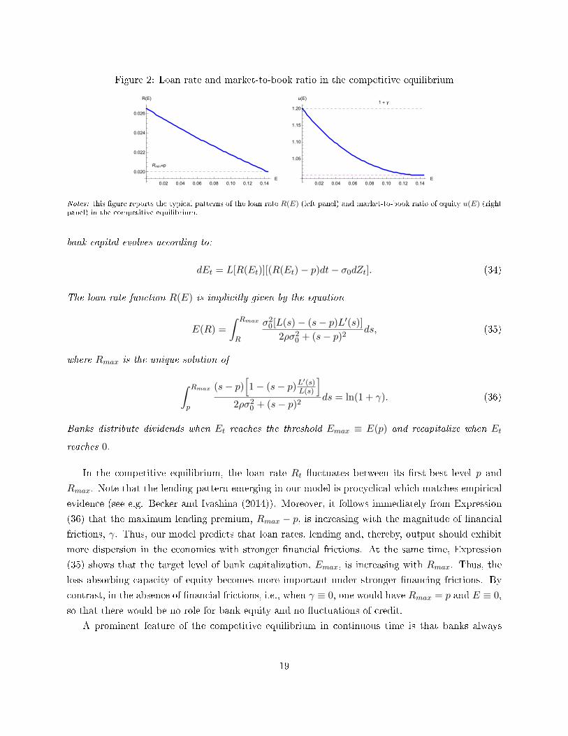
Figure 2: Loan rate and market-to-book ratio in the competitive equilibrium

0.02 0.04 0.06 0.08 0.10 0.12 0.14E

0.020

0.022

0.024

0.026

R(E)

0.02 0.04 0.06 0.08 0.10 0.12 0.14E

1.05

1.10

1.15

1.20

u(E)1 + γ

Rmin=p

Notes: this �gure reports the typical patterns of the loan rate R(E) (left panel) and market-to-book ratio of equity u(E) (rightpanel) in the competitive equilibrium.

bank capital evolves according to:

dEt = L[R(Et)][(R(Et)− p)dt− σ0dZt]. (34)

The loan rate function R(E) is implicitly given by the equation

E(R) =

∫ Rmax

R

σ20[L(s)− (s− p)L′(s)]

2ρσ20 + (s− p)2

ds, (35)

where Rmax is the unique solution of

∫ Rmax

p

(s− p)[1− (s− p)L

′(s)L(s)

]2ρσ2

0 + (s− p)2ds = ln(1 + γ). (36)

Banks distribute dividends when Et reaches the threshold Emax ≡ E(p) and recapitalize when Et

reaches 0.

In the competitive equilibrium, the loan rate Rt �uctuates between its �rst-best level p and

Rmax. Note that the lending pattern emerging in our model is procyclical which matches empirical

evidence (see e.g. Becker and Ivashina (2014)). Moreover, it follows immediately from Expression

(36) that the maximum lending premium, Rmax − p, is increasing with the magnitude of �nancial

frictions, γ. Thus, our model predicts that loan rates, lending and, thereby, output should exhibit

more dispersion in the economies with stronger �nancial frictions. At the same time, Expression

(35) shows that the target level of bank capitalization, Emax, is increasing with Rmax. Thus, the

loss absorbing capacity of equity becomes more important under stronger �nancing frictions. By

contrast, in the absence of �nancial frictions, i.e., when γ ≡ 0, one would have Rmax = p and E ≡ 0,

so that there would be no role for bank equity and no �uctuations of credit.

A prominent feature of the competitive equilibrium in continuous time is that banks always

19

postpone recapitalizations until Emin = 0.27 This marks a sharp di�erence with respect to the

discrete-time version of the model, in which recapitalizations occur at a strictly positive level of ag-

gregate equity. The explanation for this feature is closely linked to the fact that, when banks have a

possibility to instantaneously adjust lending and aggregate losses are small (which is implied by the

di�usion process), the constrained region [Emin, E) identi�ed in the discrete-time set-up shrinks to

a single point, {Emin} (this is proven in Appendix B).28 However, since the bene�t of accelerating

recapitalization disappears in this case (i.e., shareholders no longer bear the �shadow costs� asso-

ciated with the market leverage constraint), it also becomes optimal to postpone recapitalizations

until the last moment.

4.2 Long run behavior of the economy

We now exploit the continuous-time version of the model to study the long-run behavior of

the economy in the competitive equilibrium. To this end, we look at the long-run behavior of the

loan rate.29 Note that the loan rate function R(E) cannot generally be obtained in closed form.

However, it turns out that the dynamics of the loan rate Rt = R(Et) is explicit. Indeed, applying

Itô's lemma to Rt = R(Et) yields:

dRt = L[R(Et)]

((R(Et)− p)R′(Et) +

σ20L[R(Et)]

2R′′(Et)

)︸ ︷︷ ︸

µ(Rt)

dt−σ0L[R(Et)]R′(Et)︸ ︷︷ ︸

σ(Rt)

dZt. (37)

After some computations involving the use of Expression (31), one can obtain the drift and the

volatility of Rt = R(Et) in closed form. This yields the following proposition:

27However, the property Emin = 0 is not a general feature of the continuous-time set-up. In the (unreported)version of our model in which the dynamics of equity follows a jump process, the constrained region (on which themarket-based leverage constraint binds) does not vanish and, as a result, banks recapitalize at a strictly positive levelof aggregate capital. Moreover, even in the di�usion set-up, the property Emin = 0 may not hold if one allows for atime-varying �nancing cost. In Appendix F we allow γ to switch between two values γG (Good state) and γB (Badstate) such that γB > γG. Our numerical analysis reveals that, when γB is very high, in the Good state banks willraise new equity at a strictly positive level of E in order to reduce the probability of incurring larger �nancing costsconditional on a sudden transition to the Bad state. This result is in line with the �market timing� e�ect that was �rstidenti�ed in the dynamic setting by Bolton et al. (2013) in the context of a partial-equilibrium liquidity-managementmodel with the time-varying �xed cost of recapitalization.

28This feature echoes the result obtained in the model by Biais et al. (2007) in the context of a principal-agentmodel. In particular, they show that the region on which the project has to be downsized in discrete time shrinks toa single point in the continuous-time limit.

29One could equivalently look at the dynamics of the state variable Et. However, in this simple set-up with noregulation, working with Rt instead of Et enables us to provide an analytic characterization of the system's behavior,because the drift and volatility of Rt have closed-form expressions. By contrast, the drift and volatility of the processEt cannot in general be obtained in closed form, since R(E) has an explicit expression only for particular speci�cationsof the credit demand function.

20

Proposition 3 The loan rate Rt = R(Et) has explicit dynamics

dRt = µ(Rt)dt+ σ(Rt)dZt, p ≤ Rt ≤ Rmax, (38)

with re�ections at both ends of the support. The volatility function is given by

σ(R) =2ρσ2

0 + (R− p)2

σ0

(1− (R− p)L

′(R)L(R)

) . (39)

The drift function is

µ(R) = σ(R)h(R)

2, (40)

where

h(R) =σ(p)− σ(R)

R− p− R− p

σ0+ σ′(R). (41)

The impulse response methodology that is usually employed to study the long-run dynamics

in the traditional macro models consists in simulating the dynamics of a model after a single

unanticipated shock at t = 0. In our model, this would correspond to the particular trajectory of

the Brownian motion dZt ≡ 0 for t > 0, which yields dRt = µ(Rt)dt. It can be shown that µ(p) = 0,

so that the �rst best rate Rfb = p is a steady state of this deterministic system. In Appendix E

we study the properties of the deterministic steady-state and demonstrate that it is generally not

stable. Moreover, we show below that this "deterministic" steady state does not provide a correct

picture of the asymptotic behavior of the economy, as the latter is mainly driven by the endogenous

risk σ(R) neglected by the impulse response analysis.

Given the loan rate dynamics de�ned in Proposition 3, the assymptotic behavior of the economy

can be described by the ergodic density function which measures the average time spent in the

neighborhood of each possible loan rate R: the states with low R (equivalently, high aggregate

capital E) can be interpreted as "boom" states and the states with high R (equivalently, low

aggregate capital E) can be thought of as "bust" states. This ergodic density function can be

computed by solving the Kolmogorov forward equation (see Appendix A for details).

Proposition 4 The competitive loan rate process Rt is ergodic. Its asymptotic distribution is char-

acterized by the probability density function

g(R) =C0

σ2(R)exp(∫ R

p

2µ(s)

σ2(s)ds), (42)

where the constant C0 is such that∫ Rmaxp g(R)dR = 1.

21

By di�erentiating the logarithm of the ergodic density de�ned in (42), we obtain:

g′(R)

g(R)=

2µ(R)

σ2(R)− 2σ′(R)

σ(R). (43)

Using the general formulas for σ(R) and µ(R), it can be shown that σ(p) = 2ρσ0, σ′(p) =

2ρσ0L′(p)L(p) < 0 and µ(p) = 0. Hence, g′(p) > 0, which means that the state R = p that would

correspond to the "deterministic" steady state is de�nitely not the one at which the economy

spends most of the time in the stochastic set up. To get a deeper understanding of the determinants

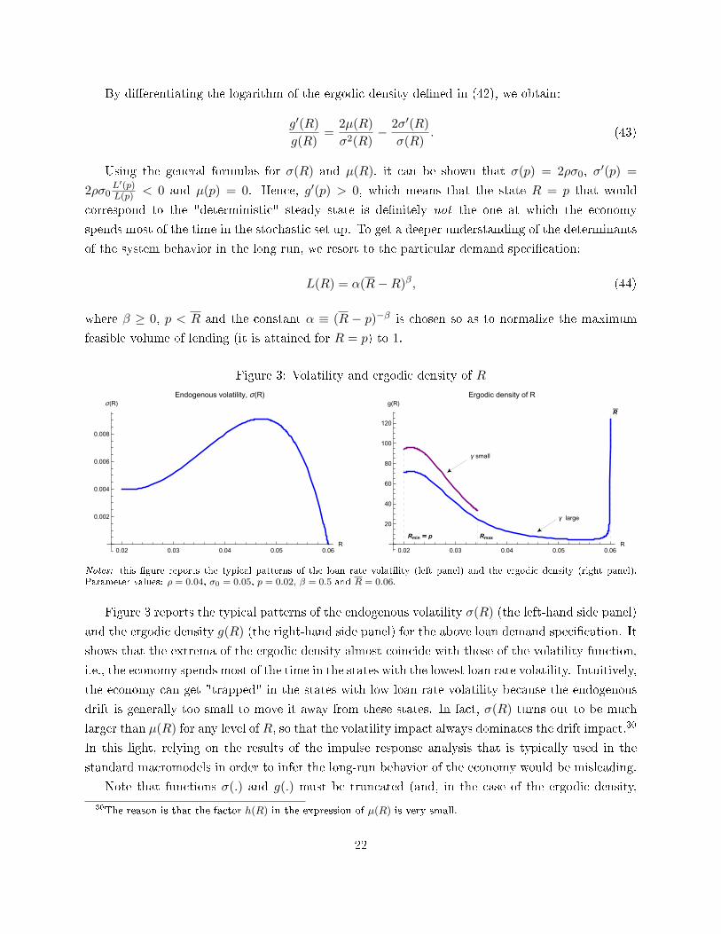
of the system behavior in the long run, we resort to the particular demand speci�cation:

L(R) = α(R−R)β, (44)

where β ≥ 0, p < R and the constant α ≡ (R − p)−β is chosen so as to normalize the maximum

feasible volume of lending (it is attained for R = p) to 1.

Figure 3: Volatility and ergodic density of R

0.02 0.03 0.04 0.05 0.06R

0.002

0.004

0.006

0.008

σ(R)

Endogenous volatility, σ(R)

0.02 0.03 0.04 0.05 0.06R

20

40

60

80

100

120

g(R)

Ergodic density of R

Rmax

R

γ small

γ large

Rmin p

Notes: this �gure reports the typical patterns of the loan rate volatility (left panel) and the ergodic density (right panel).Parameter values: ρ = 0.04, σ0 = 0.05, p = 0.02, β = 0.5 and R = 0.06.

Figure 3 reports the typical patterns of the endogenous volatility σ(R) (the left-hand side panel)

and the ergodic density g(R) (the right-hand side panel) for the above loan demand speci�cation. It

shows that the extrema of the ergodic density almost coincide with those of the volatility function,

i.e., the economy spends most of the time in the states with the lowest loan rate volatility. Intuitively,

the economy can get "trapped" in the states with low loan rate volatility because the endogenous

drift is generally too small to move it away from these states. In fact, σ(R) turns out to be much

larger than µ(R) for any level of R, so that the volatility impact always dominates the drift impact.30

In this light, relying on the results of the impulse response analysis that is typically used in the

standard macromodels in order to infer the long-run behavior of the economy would be misleading.

Note that functions σ(.) and g(.) must be truncated (and, in the case of the ergodic density,

30The reason is that the factor h(R) in the expression of µ(R) is very small.

22

rescaled) on [p,Rmax], where Rmax depends on the magnitude of the maximum level of issuing costs

γ. For the speci�cation of the loan demand function stated in (44) we always have Rmax < R.31

However, Rmax can be arbitrary close to R, which typically happens with very strong �nancial

frictions and low elasticity of credit demand. In that case the economy will spend quite some time

in the region where the loan rate is close to Rmax. We interpret this situation as a persistent "credit

crunch": it manifests itself via scarce bank equity capital, high loan rates, low volumes of lending

and output.

This "credit crunch" scenario is reminiscent to the "net worth trap" documented by Brunner-

meier and Sannikov (2014).32 In their model, the economy may fall into a recession because of the

ine�cient allocation of productive capital between more and less productive agents, which they call

�experts� and �households� respectively. This allocation is driven by the dynamics of the equilibrium

price of capital, which depends on the fraction of the total net worth in the economy that is held by

experts. After experiencing a series of negative shocks on their net worth, experts have to sell capital

to less productive households, so that the average productivity in the economy declines. Under a

reduced scale of operation, experts may struggle for a long time to rebuild net worth, so that the

economy may be stuck in a low output region. In our model, the output in the economy is driven by

the volume of credit that entrepreneurs can get from banks, whereas the cost of credit depends on

the level of aggregate bank capitalization. When the banking sector su�ers from a series of adverse

aggregate shocks, its loss absorbing capacity deteriorates. As a result, the ampli�cation mechanism

working via the market-to-book value becomes more pronounced and bankers thus require a larger

lending premium. The productive sector reacts by reducing its demand for credit and the banks

have to shrink their scale of operations, which makes it even more di�cult to rebuild equity capital.

4.3 Ine�ciencies

In this section we show that the competitive equilibrium is not constrained e�cient due to

a pecuniary externality that each bank imposes on its competitors. More precisely, competitive

banks do not take into account the e�ect of their individual lending decisions on the dynamics of

aggregate bank equity. This leads to excessive lending when banks are poorly capitalized, implying

overexposure of the banking sector to aggregate shocks and the erosion of its ability to accumulate

earnings.

We organize our discussion as follows. First we evaluate social welfare in the competitive equi-

librium. Then we analyze the second best allocation in the set-up with completely inelastic demand

for loans, which allows us to isolate the ine�ciencies caused by excessive exposure of the banking

sector to aggregate shocks. Finally, we turn to the more general case with downward sloping loan

demand where, in addition to overexposure of the banking sector, a second, distributive ine�ciency

31To prove this property, it is su�cient to show that the integral∫ Rp

(R−p)H(R)

σ20L(R)

dR diverges.32In a partial equilibrium set-up, a similar result is found by Isohätälä, Milne and Robertson (2014).

23

comes into play: Allowing banks to make more pro�ts can be socially desirable even though this

reduces �rm pro�ts, in particular, if the banking sector is poorly capitalized.

4.3.1 Welfare in the competitive equilibrium

Social welfare in our framework can be computed as the expected value of households' total dis-

counted consumption, i.e., discounted �rm pro�ts, which are immediately distributed to households,

plus the present value of banks' expected dividend payments net of expected capital injections:33

W (E) = E[∫ +∞

0e−ρt (πF (K) + d∆t − (1 + γ) dIt)|E0 = E

], (45)

where πF (K) ≡ F (K) −KF ′ (K) denotes the aggregate instantaneous production of �rms net of

credit costs.

By using aggregate bank equity E as a state variable, we can apply standard methods to com-

pute the social welfare function. As long as banks neither distribute dividends nor recapitalize,

households' consumption consists only of �rm pro�ts. Therefore, in the region E ∈ (0, Emax),34 the

social welfare function, W (E), must satisfy the following di�erential equation:35

ρW (E) = F (K)−K(E)F ′(K) +K(F ′(K)− p

)W ′(E) +

σ20

2K2W ′′(E), (46)

subject to the boundary conditions:

W ′(0) = 1 + γ, (47)

W ′(Emax) = 1. (48)

The above boundary conditions re�ect the fact that dividend distribution and bank recapitalization

only a�ect the market value of banks, without producing any immediate impact on the �rms' pro�t.

Before solving for the constrained welfare optimum in the next subsection, we �rst evaluate the

social welfare function at the competitive equilibrium in order to get a �rst grasp of the prevailing

distortions. To this end, we take the �rst derivative of the right-hand side of equation (46) with

respect to K. Since we are interested in the impact of a marginal increase in lending on welfare

at the competitive equilibrium, we substitute the competitive loan rate from equilibrium condition

33In our welfare analysis, we neglect the value generated by deposits as it does not depend on aggregate bank

capitalization. It can easily be accounted for by adding a constant term λ(D)−Dλ′(D)ρ

to W (E).34As will be shown below, also when bank policies are dictated by the social planner, the optimal dividend and

recapitalization policies are of the barrier type.35For the sake of space, we omit the argument of K(E).

24

(27) into the derivative to get:

F ′′(K)K[W ′(E)− 1

]+W ′(E)

[W ′′(E)

W ′(E)− u′(E)

u(E)

]σ2

0K. (49)

Note that expression (49) is equivalent to expression (21) that we have encountered in the

discrete-time version of the model. The �rst term in (49) sheds light on the distributive ine�ciency:

An increase in aggregate lending drives down the loan rate (F ′′(K) = ∂R/∂K < 0). This increases

�rms' pro�ts but bites into the pro�ts of banks and, thus, impairs the banks' ability to accumulate

loss absorbing capital in the form of retained earnings.36 As long as the (social) marginal value

of aggregate equity, W ′(E), is larger than one, welfare could be improved by restricting the total

volume of lending below its competitive level. This is true at least when aggregate equity is low

and thus its marginal (social) value is high (recall that W ′(0) = 1 + γ).

The second term in (49) captures the ine�ciency stemming from the fact that competing banks

do not take into account how their individual lending decisions a�ect the exposure of the banking

sector to aggregate shocks. The term in square brackets captures the di�erence between the so-

cial planners and individual banks' e�ective risk aversion with respect to variations in aggregate

capital.37

Yet, without making further assumptions, both terms in (49) cannot be signed globally. We now

turn to the case with inelastic demand (F ′′(K) = 0) in order to isolate the impact of the second

term in (49), thereby, focusing on the ine�cient exposure of the banking sector to aggregate shocks.

4.3.2 Inelastic demand

This subsection assumes that the �rms' demand for loans is constant and equal to 1 as long as

the loan rate does not exceed some maximum rate R:38

L (R) =

1 for R ≤ R,

0 for R > R.(50)

This speci�cation leads to closed-form solutions for the value functions, loan volumes and loan rates

for both the competitive and the second-best allocations.

In the competitive equilibrium, banks always lend at the maximum feasible scale L(R) = 1 as

36This "margin e�ect" of competition is also acknowledged in Martinez-Miera and Repullo (2010) albeit in anentirely di�erent application.

37Recall from (27) that banks' risk-aversion determines the size of "lending premium" for an aggregate level oflending K.

38This loan demand speci�cation can be obtained from the demand speci�cation (44) by taking the limit caseβ ≡ 0.

25

long as R(E) in condition (27) does not exceed R and, thus,39

KCE(E) = 1.

Then, by using the results of Proposition 2, one can obtain the explicit characterization of the

competitive equilibrium. In particular, the equilibrium loan rate can be found in closed-form:

RCE(E) = p+√

2ρσ0 tan[√2ρ

σ0(Emax − E)

].

Moreover, solving Equation (36) yields a closed form for the maximum interest rate that prevails

upon recapitalization,

RCEmax = p+ σ0

√2ρ(2γ + γ2),

and the target level of aggregate equity is given by

ECEmax =σ0√2ρ

arctan√

2γ + γ2.

We now analyze the second best allocation, that is, the welfare maximizing policies subject to

the same constraint as in the competitive equilibrium, i.e., that issuing new capital is costly.

W (E) = maxR,K,d∆,dI

E[∫ +∞

0e−ρt (πF (Kt, Rt) + d∆t − (1 + γ) dIt)|E0 = E

], (51)

where the instantaneous �rms' pro�t is given by πF (Kt, Rt) = Kt(R−Rt). The single state variablein the social planner's problem is aggregate bank equity E and the market for bank credit must

clear, i.e., Kt = L(Rt). Assuming that the welfare function is concave (this is veri�ed ex-post), it

is immediate that optimal dividend and recapitalization policies are of the �barrier type� and thus

aggregate equity �uctuates within a bounded support [ESBmax, ESBmax], over which the social welfare

function satis�es the ODE

ρW (E) = maxR≤R,K≤1

K(R−R) +K(R− p)W ′(E) +σ2

0K2

2W ′′(E). (52)

It can be established that ESBmin = 0 and that the optimal dividend barrier ESBmax is given by the

super-contact condition

W ′′(ESBmax) = 0. (53)

As a consequence, it holds that W ′(E) > 1 for E ∈ [0, ESBmax), implying that social welfare

is maximized at the highest possible ("reservation") loan rate RSB(E) = R. Therefore, �rms'

pro�ts will be equal to zero and the social welfare function coincides with the value function of a

39To ensure that a competitive equilibrium exists we make the implicit assumption that R ≥ RCEmax.

26

monopolistic bank, satisfying the ODE40

ρW (E) = maxK≤1

K(R− p

)W ′(E) +

σ20K

2

2W ′′(E). (54)

Maximizing the right-hand side of the above equation with respect to the aggregate lending

volume K yields:

KSB(E) = min

{1,

(R− p

)σ2

0

(−W

′′(E)

W ′(E)

)−1}. (55)

Note that this condition shares some similarities with condition (27) in the competitive equilib-

rium, with the notable di�erence that loan supply depends on the social implied risk aversion with

respect to variation in aggregate equity, −W ′′(E)/W ′(E), whereas in the competitive equilibrium,

banks' inverse supply R is driven by the private implied risk aversion −u′(E)/u(E). Substituting

KSB back into (54) implies that for interior loan volumes (KSB < 1), the social welfare function

has an explicit solution

W1(E) = c2

(E

a− c1

)η, (56)

where η ≡ 2ρσ20

(R−p)2+2ρσ20

and {c1, c2} are constants to be determined.41

Substituting the general solution of the welfare function (56) into Equation (55) shows that the

optimal volume of lending, if interior, linearly increases with aggregate capital E:

KSB(E) = min

{1,

2ρ

R− p

(E

a− c1

)}. (57)

Let EK denote the critical level of aggregate capital that satis�es

KSB(EK) = 1, (58)

such that the welfare maximizing loan volume satis�es KSB(E) < 1 for E < EK and KSB(E) = 1

for E ≥ EK .42 That is, for low levels of aggregate bank capital, the social planner restricts aggregate

lending below the level that is attained in the competitive equilibrium. The reason for this is that,

in the competitive equilibrium, each bank maximizes its pro�ts, taking the aggregate capitalization

of the banking sector as given. In particular, banks do not take into account how their individual

lending decisions a�ect the banking sector's exposure to common productivity shocks (i.e., the

endogenous volatility of aggregate bank capital).

40In the setting with inelastic demand social welfare coincides with the market value of a monopolistic bank.However, this result does not extend to the more realistic cases where demand for loans is elastic.

41We indicate the solution by W1 in order to di�erentiate it from its counterpart W2 in the region where the cornersolution R = 1 applies.

42Note that EK does not need to be positive, in which case KSB(E) = 1 for all E ∈[ESBmin, E

SBmax

]. This scenario

might materialize for relatively low values of γ and σ0.

27

Consider now the region (EK , ESBmax], in which the social planner would allow the banking sector

to operate at the maximum feasible scale, i.e., KSB(E) = 1. Substituting KSB(E) = 1 into (54)

and solving the obtained ODE under the boundary conditions (48) and (53), yields the explicit

solution of the welfare function for E ∈ (EK , ESBmax],

W2(E) =1

β1 − β2

[β2

β1eβ1(E−ESBmax) +

β1

β2eβ2(E−ESBmax)

], (59)

where β1 > 0 and β2 < 0 are the roots of the characteristic equation ρ = (R− p)β +σ2

02 β

2.43

Piecing two regions together, we require the continuity of the welfare function and its �rst

derivative at the critical threshold EK , i.e.,

W1(EK) = W2(EK), (60)

W ′1(EK) = W ′2(EK). (61)

We are thus left with four conditions (47), (58), (60), and (61), which allows us to determine the

four remaining unknowns c1, c2, EK , and ESBmax.

Figure 4 illustrates the optimal loan rate (the left-hand side panel) and lending (the right-hand

side panel) in the competitive equilibrium (CE) and in the second best (SB). In the second best

allocation, banks lend (weakly) less than in the competitive equilibrium, which re�ects the pecuniary

externality in�icted by each bank on its competitors. The social planner internalizes this externality

and reduces the exposure to macro shocks (σ0K(E)), in the states of the world where the implied

risk aversion with respect to �uctuations in E is most severe (i.e., close to the recapitalization barrier

Emin = 0). Moreover, note that, while in the second best, the optimal loan rate is always equal

to the maximum rate R, in the competitive setting, it is strictly decreasing in aggregate equity.

As a result, the instantaneous pro�t of the banking sector in the second best allocation is larger

than in the competitive equilibrium, which makes it easier for banks to rebuild equity bu�ers after

negative shocks. Thus, the second best allocation implies lower risk exposure and higher margins.

This implies a somewhat counterintuitive result: the optimal target equity bu�ers in the second

best allocation are smaller than in the competitive equilibrium, i.e., ESBmax < ECEmax.

4.3.3 Linear demand

We now turn to the example of a linear demand for loans. To this end, we consider the loan

demand speci�cation introduced in (44) with β = 1, i.e.,

L(R) =R−RR− p

.

43In particular, we have β1,2 = −R−p±√

(R−p)2+2ρσ20

σ20

.

28

Figure 4: Loan rate and credit volume under inelastic loan demand: CE vs SB

0.05 0.10 0.15E

0.04

0.06

0.08

0.10

R(E)

RCE RSB

0.00 0.05 0.10 0.15E

0.7

0.8

0.9

1.0

K(E)

KCE KSB

EmaxSB

EmaxEmaxSB

Emax

Notes: this �gure reports the typical patterns of the loan rates (the left-hand side panel) and credit volumes (the right-handside panel) in the competitive equilibrium (dash-dotted line) and the second best allocation (solid line). Parameter values:ρ = 0.05, σ0 = 0.05, p = 0.02, γ = 2, R = 0.1, β = 0.

The second best lending strategy can be de�ned as the solution to the following Bellman equation

ρW (E) = maxK≥0

(R− p)K2

2+K(1−K)(R− p)W ′(E) +

σ20

2K2W ′′(E), (62)

subject to the boundary conditions W ′(0) = 1 + γ and W ′(ESBmax) = 1. The optimal dividend

barrier ESBmax satis�es W′′(ESBmax) = 0. The �rst-order condition of the above maximization problem

determines the optimal level of lending:44

KSB(E) =(R− p)W ′(E)

(R− p)[2W ′(E)− 1]− σ20W

′′(E).

With elastic demand, social welfare does no longer coincide with the value of a monopolistic bank.

Therefore, let us consider the latter as another benchmark. The value function of a monopolistic

bank, V (E), satis�es the Bellman equation

ρV (E) = maxK≥0

K(1−K)(R− p)V ′(E) +σ2

0

2K2V ′′(E), (63)

which di�ers from (62) only by the fact that the �rms' pro�ts do not show up in the Bellman

equation.

The optimal level of lending chosen by a monopolistic bank is given by

KMonop(E) =(R− p)V ′(E)

2(R− p)V ′(E)− σ20V′′(E)

,

44It is easy to see that, at the target level of aggregate bank equity, ESBmax, that satis�es equations W′(ESBmax) = 1

and W ′′(ESBmax) = 0, we have RSB(ESBmax) = p.

29

and the value function V (E) is a solution of the ODE:

V ′′(E) =(R− p)V ′(E)

[4ρV (E)− (R− p)V ′(E)

]2ρσ2

0V (E),

subject to the usual conditions V ′(0) = 1 + γ and V ′(EMonopmax ) = 1, with EMonop

max satisfying

V ′′(EMonopmax ) = 0.

Figure 5 contrasts the loan rate and lending functions emerging in the competitive, second best

and monopolistic settings. The qualitative insights from the inelastic case framework are still true,

albeit less clear, since now one the social planner takes into account the price depressing e�ect of

an increase in lending and the associated reallocation of pro�ts. This interference of the e�ects no

longer allows us to clearly sign the lending distortions in the competitive equilibrium. However, the

social planner still wants to restrict lending below the competitive level when E is low, even though

this reduces �rm's pro�ts. The reason is that when aggregate capital is low, the social value of bank

pro�ts (which are used to build equity bu�ers) is larger than that the value of the �rms' pro�ts

(which are consumed immediately) and also the implied risk-aversion is high. Yet, the loan rate

(lending) corresponding to the second best allocation is always lower (higher) as compared to the one

chosen in the monopolistic setting, which is a natural consequence of the fact that a monopolistic

bank does not internalize the impact of its lending decisions on the �rms' pro�ts. Moreover, in the

second best allocation, a poorly capitalized banking sector is less (more) exposed to aggregate shocks

which leads to higher (smaller) instantaneous bank pro�ts than in the competitive (monopolistic)

setting. This implies that the optimal dividend barrier under the second best allocation is smaller

(larger) than in the competitive (monopolistic) setting, i.e., EMonopmax < ESBmax < ECEmax.

Figure 5: Loan rate and credit volume under elastic loan demand: CE vs SB

0.02 0.04 0.06 0.08 0.10 0.12 0.14E

0.02

0.04

0.06

0.08

0.10

R(E)

0.02 0.04 0.06 0.08 0.10 0.12 0.14E

0.2

0.4

0.6

0.8

1.0

K(E)

RMonop

RCE

RSB

EmaxSB

EmaxEmaxMonop

KMonop

KSB

KCE

EmaxSB

EmaxEmaxMonopCE CE

Notes: this �gure reports the typical patters of the loan rates (the left-hand side panel) and credit volumes (the right-hand sidepanel) in the competitive equilibrium (dash-dotted lines), the second best allocation (solid lines) and the monopolistic setting(dashed lines). Parameter values: ρ = 0.05, σ0 = 0.05, p = 0.02, γ = 0.2, R = 0.15, β = 1.

30

5 Impact of capital regulation

So far our analysis has been focused on the "laissez-faire" environment in which banks face no

regulation. Our objective in this section is to understand the impact of capital regulation on bank

policies. Let us assume that public authorities enforce a minimum capital requirement, under which

each bank must maintain equity capital above a certain fraction of loans, i.e.,

et ≥ Λkt,

where Λ ∈ (0, 1] is the minimum capital ratio.45

Note that, under such a formulation, banks have two options to comply with minimum capital

requirements. The �rst option is to immediately recapitalize as soon as the regulatory constraint

starts binding. The second option consists in cutting on lending and simultaneously reducing deposit

taking. We show below that, in our model, banks use the �rst option when Et is small and the

second one when Et is large. In other words, a capital ratio does two things: it forces banks to

recapitalize earlier (i.e., Emin > 0) and to reduce lending as compared to the unregulated case.

To solve for the regulated equilibrium, we again start by looking at the maximization problem of

an individual bank. As in the unregulated set-up, bank shareholders maximize the market value of

their claim by choosing their lending, recapitalization and dividend policies subject to the regulatory

restriction on the volume of lending:

vΛ(e, E) ≡ euΛ(E) = maxkt≤ e

Λ,dδt,dit

E[∫ +∞

0e−ρt (dδt − (1 + γ)dit)|e0 = e, E0 = E

]. (64)

To have the intuition of the solution to the above problem, recall that, in the unregulated case,

bank recapitalizations take place only when equity is completely depleted. Thus, it is natural to

expect that the regulatory constraint will be binding for relatively low levels of equity. Indeed, in

the general case, the bank may �nd itself in one of two cases: (i) when its level of equity is relatively

high, the regulatory constraint is not binding and the volume of lending is still determined by the

�rms' demand for credit; (ii) in the states with low equity, the regulatory constraint binds and the

volume of lending is determined by kt = et/Λ. Due to the homotheticity property, at each point

in time, all banks have the same leverage ratio. Thus, it is legitimate to anticipate the existence of

the critical level of bank capital EΛc , such that the regulatory constraint binds (for all banks) for

any E ∈ [EΛmin, E

Λc ] and is slack for any E ∈ (EΛ

c , EΛmax]. This critical threshold EΛ

c must satisfy

K(EΛc )

EΛc

=1

Λ.

45Since our model only considers one type of bank assets (loans), we cannot discuss the issue of risk weights ordistinguish a leverage ratio from a risk-weighted capital ratio.

31

For Λ high enough, EΛc tends to EΛ

max and the unconstrained region disappears entirely. For future

reference, we denote the critical leverage ratio above which the unconstrained region disappears by

Λ∗.

Proposition 5 For all Λ ∈ (0, 1], there exists a unique regulated equilibrium, where the support of

Et is [EΛmin, E

Λmax]. This equilibrium is characterized by one of two regimes:

a) for Λ ≥ Λ∗, the regulatory constraint binds over the entire interval [EΛmin, E

Λmax]. The loan rate

is explicitly given by

R(Et) = L−1[Et/Λ], (65)

where L−1 is the inverse function of the loan demand. The dynamics of aggregate bank capital

is given by:dEtEt

=1

Λ

((L−1[Et/Λ]− p)dt− σ0dZt

), E ∈ (EΛ

min, EΛmax).

b) for Λ < Λ∗, the capital constraint only binds for E ∈ [EΛmin, E

Λc ] and is slack for E ∈ (EΛ

c , EΛmax],

where EΛc is a critical capitalization level. When E ∈ (EΛ

min, EΛc ], the dynamics of aggregate

equity and the loan rate function are de�ned as in the regime a). When E ∈ (EΛc , E

Λmax), the

loan rate satis�es the �rst-order di�erential equation46 R′(E) = −1/H[R(E)] with the boundary

condition R(EΛc ) = L−1[EΛ

c /Λ].

In either regime, banks distribute dividends when Et = EΛmax and recapitalize when Et = EΛ

min.

We show in Appendix A that, in the unconstrained region (EΛc , E

Λmax), the market-to-book value

still simultaneously satis�es Equations (27) and (30), whereas in the constrained region (EΛmin, E

Λc )

it satis�es instead

ρ =E(L−1[E/Λ]− p)

Λ

u′Λ(E)

uΛ(E)+σ2

0E2

2Λ2

u′′Λ(E)

uΛ(E), (66)

under the conditionu′Λ(E)

uΛ(E)≥ −L

−1[E/Λ]− pσ2

0E/Λ, (67)

with equality at E = EΛc .

The optimal recapitalization and payout decisions are characterized by two boundaries, EΛmin

(recapitalizations) and EΛmax (dividend payments), such that uΛ(EΛ

min) = 1 + γ and uΛ(EΛmax) = 1.

In Appendix C.1 we provide the detailed description of the computational procedure that enables

us to numerically solve for the regulated equilibrium.

To get general insight into the impact of capital regulation on the cost of credit and the bank's

policies, we perform a comparative static analysis by computing the equilibrium characteristics of

46The function H(.) is de�ned in (31). Thus, in the region E ∈ (EΛc , E

Λmax), the dynamics of aggregate equity is

described by the same di�erential equation as in the unregulated set-up.

32

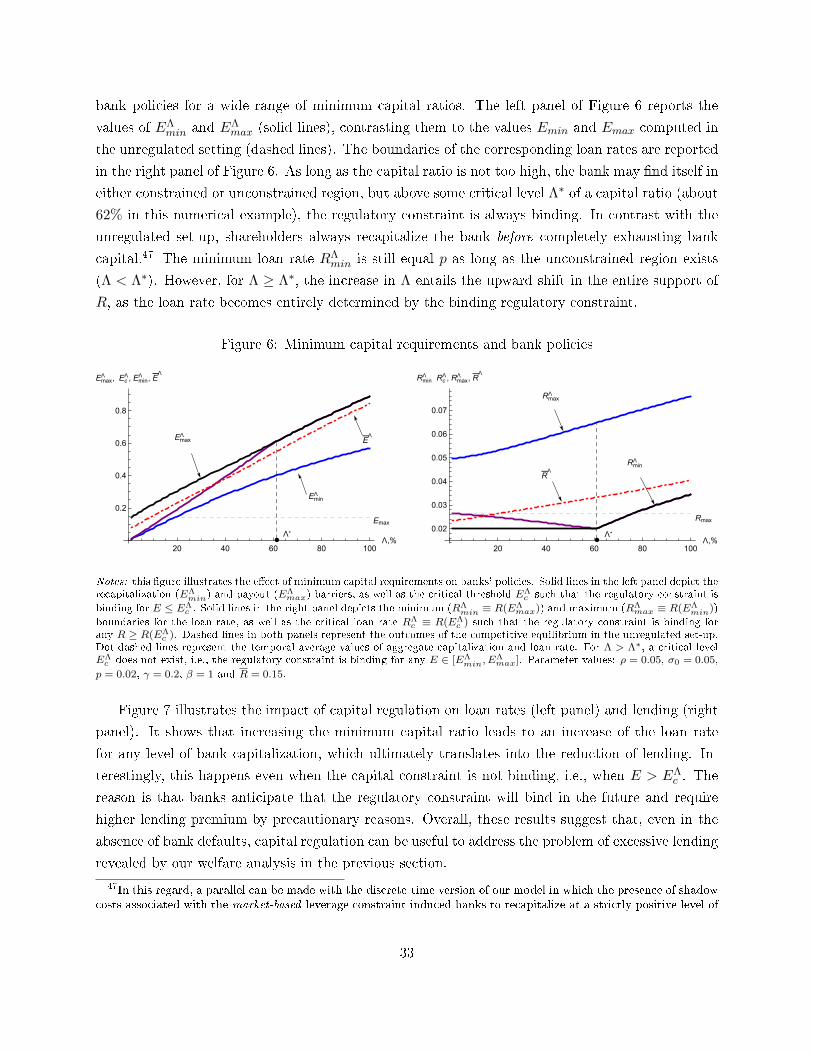
bank policies for a wide range of minimum capital ratios. The left panel of Figure 6 reports the

values of EΛmin and EΛ

max (solid lines), contrasting them to the values Emin and Emax computed in

the unregulated setting (dashed lines). The boundaries of the corresponding loan rates are reported

in the right panel of Figure 6. As long as the capital ratio is not too high, the bank may �nd itself in

either constrained or unconstrained region, but above some critical level Λ∗ of a capital ratio (about

62% in this numerical example), the regulatory constraint is always binding. In contrast with the

unregulated set-up, shareholders always recapitalize the bank before completely exhausting bank

capital.47 The minimum loan rate RΛmin is still equal p as long as the unconstrained region exists

(Λ < Λ∗). However, for Λ ≥ Λ∗, the increase in Λ entails the upward shift in the entire support of

R, as the loan rate becomes entirely determined by the binding regulatory constraint.

Figure 6: Minimum capital requirements and bank policies

20 40 60 80 100Λ,%

0.2

0.4

0.6

0.8

EmaxΛ , Ec

Λ, EminΛ , E

Λ

20 40 60 80 100Λ,%

0.02

0.03

0.04

0.05

0.06

0.07

RminΛ

RcΛ, Rmax

Λ , RΛ

Λ*Λ*

EmaxΛ

EminΛ

Emax

EΛ

RmaxΛ

Rmax

RΛ

RminΛ

Notes: this �gure illustrates the e�ect of minimum capital requirements on banks' policies. Solid lines in the left panel depict therecapitalization (EΛ

min) and payout (EΛmax) barriers, as well as the critical threshold E

Λc such that the regulatory constraint is

binding for E ≤ EΛc . Solid lines in the right panel depicts the minimum (RΛ

min ≡ R(EΛmax)) and maximum (RΛ

max ≡ R(EΛmin))

boundaries for the loan rate, as well as the critical loan rate RΛc ≡ R(EΛ

c ) such that the regulatory constraint is binding forany R ≥ R(EΛ

c ). Dashed lines in both panels represent the outcomes of the competitive equilibrium in the unregulated set-up.Dot-dashed lines represent the temporal average values of aggregate capitalization and loan rate. For Λ > Λ∗, a critical levelEΛc does not exist, i.e., the regulatory constraint is binding for any E ∈ [EΛ

min, EΛmax]. Parameter values: ρ = 0.05, σ0 = 0.05,

p = 0.02, γ = 0.2, β = 1 and R = 0.15.

Figure 7 illustrates the impact of capital regulation on loan rates (left panel) and lending (right

panel). It shows that increasing the minimum capital ratio leads to an increase of the loan rate

for any level of bank capitalization, which ultimately translates into the reduction of lending. In-

terestingly, this happens even when the capital constraint is not binding, i.e., when E > EΛc . The

reason is that banks anticipate that the regulatory constraint will bind in the future and require

higher lending premium by precautionary reasons. Overall, these results suggest that, even in the

absence of bank defaults, capital regulation can be useful to address the problem of excessive lending

revealed by our welfare analysis in the previous section.

47In this regard, a parallel can be made with the discrete-time version of our model in which the presence of shadowcosts associated with the market-based leverage constraint induced banks to recapitalize at a strictly positive level of

33

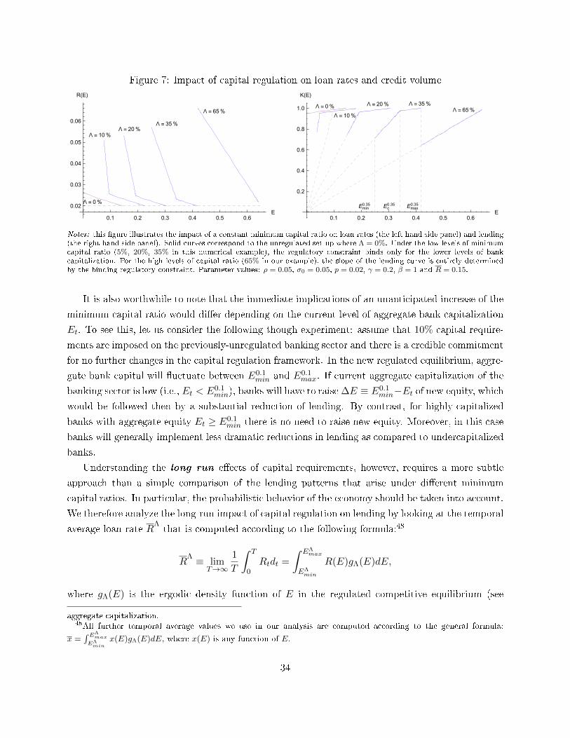
Figure 7: Impact of capital regulation on loan rates and credit volume

0.1 0.2 0.3 0.4 0.5 0.6E

0.02

0.03

0.04

0.05

0.06

R(E)

0.1 0.2 0.3 0.4 0.5 0.6E

0.2

0.4

0.6

0.8

1.0

K(E)

Λ = 0%

Λ = 10%

Λ = 35%Λ = 20%

Λ = 65%Λ = 0%

Λ = 10%

Λ = 35%Λ = 20%Λ = 65%

Ec0.35

Emax0.35

Emin0.35

Notes: this �gure illustrates the impact of a constant minimum capital ratio on loan rates (the left hand side panel) and lending(the right hand side panel). Solid curves correspond to the unregulated set-up where Λ = 0%. Under the low levels of minimumcapital ratio (5%, 20%, 35% in this numerical example), the regulatory constraint binds only for the lower levels of bankcapitalization. For the high levels of capital ratio (65% in our example), the slope of the lending curve is entirely determinedby the binding regulatory constraint. Parameter values: ρ = 0.05, σ0 = 0.05, p = 0.02, γ = 0.2, β = 1 and R = 0.15.

It is also worthwhile to note that the immediate implications of an unanticipated increase of the

minimum capital ratio would di�er depending on the current level of aggregate bank capitalization

Et. To see this, let us consider the following though experiment: assume that 10% capital require-

ments are imposed on the previously-unregulated banking sector and there is a credible commitment

for no further changes in the capital regulation framework. In the new regulated equilibrium, aggre-

gate bank capital will �uctuate between E0.1min and E0.1

max. If current aggregate capitalization of the

banking sector is low (i.e., Et < E0.1min), banks will have to raise ∆E ≡ E0.1

min−Et of new equity, which

would be followed then by a substantial reduction of lending. By contrast, for highly-capitalized

banks with aggregate equity Et ≥ E0.1min there is no need to raise new equity. Moreover, in this case

banks will generally implement less dramatic reductions in lending as compared to undercapitalized

banks.

Understanding the long run e�ects of capital requirements, however, requires a more subtle

approach than a simple comparison of the lending patterns that arise under di�erent minimum

capital ratios. In particular, the probabilistic behavior of the economy should be taken into account.

We therefore analyze the long-run impact of capital regulation on lending by looking at the temporal

average loan rate RΛthat is computed according to the following formula:48

RΛ ≡ lim

T→∞

1

T

∫ T

0Rtdt =

∫ EΛmax

EΛmin

R(E)gΛ(E)dE,

where gΛ(E) is the ergodic density function of E in the regulated competitive equilibrium (see

aggregate capitalization.48All further temporal average values we use in our analysis are computed according to the general formula:

x =∫ EΛ

max

EΛmin

x(E)gΛ(E)dE, where x(E) is any function of E.

34

Appendix C.2 for the computational details).

The dash-dotted line in the right hand side panel of Figure 6 corresponds to the typical pattern

of the temporal average loan rate RΛ. It shows that, as Λ goes up, R

Λincreases but tends to

the lower boundary of feasible loan rates, RΛmin. In other words, even though a higher minimum

capital ratio induces a substantial shift of the feasible range of the loan rates, its long-run impact

on lending is rather moderate. To understand this result, it is instructive to consider the e�ect

of higher minimum capital ratios on the temporal average level of bank capitalization, EΛ, that is

depicted by the dash-dotted line in the left-hand side panel of Figure 6. Its pattern (converging to

the dividend barrier EΛmax when Λ goes up) suggests that, under tighter capital requirements, the

banking sector becomes more stable so as in the long run banks spend more times in the states with

abundant capital.

To properly measure the e�ect of capital requirements on the stability of the banking sector,

we compute the expected time to reach49 the recapitalization barrier starting from the temporal

average level of aggregate capitalization EΛ. Figure 8 depicts the typical pattern of this stability

measure as the function of Λ, suggesting that increasing the minimum capital ratio enhances the

stability of the banking sector.

A substantial body of the existing literature attributes the stability e�ect of higher capital

requirements to the reduction in the moral hazard incentives on the banks' side (see e.g., Martinez-

Miera and Suarez (2014), Nguyên (2014)). To understand why higher minimum capital ratios

help promote �nancial stability in our setting (which completely abstracts from a moral hazard

problem), it is important to emphasize that the primary e�ect of the enhanced capital requirements

on banks' policies in the presence of �nancing frictions manifests itself via the reduction in lending.

In this regard, minimum capital regulation can be seen as a tool addressing the problem of excessive

lending by competitive banks that was discussed in Section 4.3 (i.e., by using the minimum capital

regulation, the social planner can implicitly control the endogenous volatility of aggregate capital).

Under higher minimum capital requirements, banks have lower exposure to aggregate shocks and,

at the same time, charge higher loan rates, which makes it easier for them to recover after the series

of negative shocks. This enables banks to spend more time in the states with higher aggregate

capitalization and thus relatively lower loan rates (within the feasible corridor). By reducing the

temporal average loan rate in the long run, the positive e�ect from enhanced �nancial stability

ultimately mitigates the direct negative impact in�icted by higher capital requirements on lending.

6 Conclusion

This paper develops a general equilibrium model of commercial banking, in which banks satisfy

households' needs for safe deposits and channel funds to the productive sector. Bank capital plays

49See Appendix C.3 for computational details.

35

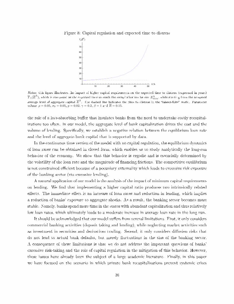
Figure 8: Capital regulation and expected time to distress

10 20 30 40 50Λ,%

10

20

30

40

50

60

70

Tγ(EΛ)

Notes: this �gure illustrates the impact of higher capital requirements on the expected time to distress (expressed in years)

T γ(EΛ

), which is computed as the expected time to reach the recapitalization barrier EΛmin, while starting from the temporal

average level of aggregate capital EΛ. The dashed line indicates the time to distress in the �laissez-faire� world. Parameter

values: ρ = 0.05, σ0 = 0.05, p = 0.02, γ = 0.2, β = 1 and R = 0.15.

the role of a loss-absorbing bu�er that insulates banks from the need to undertake costly recapital-

izations too often. In our model, the aggregate level of bank capitalization drives the cost and the

volume of lending. Speci�cally, we establish a negative relation between the equilibrium loan rate

and the level of aggregate bank capital that is supported by data.

In the continuous-time version of the model with no capital regulation, the equilibrium dynamics

of loan rates can be obtained in closed form, which enables us to study analytically the long-run

behavior of the economy. We show that this behavior is ergodic and is essentially determined by

the volatility of the loan rate and the magnitude of �nancing frictions. The competitive equilibrium

is not constrained e�cient because of a pecuniary externality which leads to excessive risk exposure

of the banking sector (via excessive lending).

A natural application of our model is the analysis of the impact of minimum capital requirements

on lending. We �nd that implementing a higher capital ratio produces two intrinsically related

e�ects. The immediate e�ect is an increase of loan rates and reduction in lending, which implies

a reduction of banks' exposure to aggregate shocks. As a result, the banking sector becomes more

stable. Namely, banks spend more time in the states with abundant capitalization and thus relatively

low loan rates, which ultimately leads to a moderate increase in average loan rate in the long run.

It should be acknowledged that our model su�ers from several limitations. First, it only considers

commercial banking activities (deposit taking and lending), while neglecting market activities such

as investment in securities and derivatives trading. Second, it only considers di�usion risks that

do not lead to actual bank defaults, but merely �uctuations in the size of the banking sector.

A consequence of these limitations is that we do not address the important questions of banks'

excessive risk-taking and the role of capital regulation in the mitigation of this behavior. However,

these issues have already been the subject of a large academic literature. Finally, in this paper

we have focused on the scenario in which private bank recapitalizations prevent systemic crises

36

from happening. A potential direction of further investigations would be to explore the alternative

scenario, where shareholders do not spontaneously inject new capital, and public authorities are

forced to intervene.

37

Appendix A. Proofs

Proof of Lemma 1. The utility of the representative consumer is

U = C0 +E[C1] + λ(D)

1 + ρ,

where the consumptions at t = 0 and t = 1 are given by aggregate budget constraints:

C0 = w0 −D − (1 + γ)I,

C1 = (1 + rD)D + πB,

where πB denotes the aggregate pro�ts of banks. Inserting the expressions of C0 and C1 into Uyields

U = w0 − (1 + γ)I +E[πB]

1 + ρ+

(rD − ρ)D + λ(D)

1 + ρ.

The �rst-order condition with respect to D immediately yields λ′(D) = ρ− rD. Q.E.D.

Proof of Lemma 2. Omitted.

Proof of Proposition 1. Omitted.

Proof of Proposition 2. By the standard dynamic programming arguments, shareholder valuev(e, E) must satisfy the Bellman equation:50

ρv = maxk≥0,dδ≥0,di≥0

{dδ(1− ve)− di(1 + γ − ve)

+ k[(R(E)− p)ve + σ20K(E)veE ] +

k2σ20

2vee

+K(E)(R(E)− p)vE +σ2

0K2(E)

2vEE

}.

(A1)

Using the fact that v(e, E) = eu(E), one can rewrite the Bellman equation (A1) as follows:

ρu(E) = maxk≥0,dδ≥0,di≥0

{dδe

[1− u(E)]− di

e[1 + γ − u(E)]

+k

e[(R(E)− p)u(E) + σ2

0K(E)u′(E)]

+K(E)(R(E)− p)u′(E) +σ2

0K2(E)

2u′′(E)

}.

(A2)

A solution to the maximization problem in k only exists when

u′(E)

u(E)≤ −R(E)− p

σ20K(E)

, (A3)

with equality when k > 0.

50For the sake of space, we omit the arguments of function v(e, E).

38

Under conjecture that R(E) ≥ p (which will be veri�ed ex-post), it follows from the aboveexpression that u(E) is a decreasing function of E. Then, the optimal payout policy maximizingthe right-hand side of (A2) is characterized by a critical barrier Emax satisfying

u(Emax) = 1, (A4)

and the optimal recapitalization policy is characterized by a barrier Emin such that

u(Emin) = 1 + γ. (A5)

In other words, dividends are only distributed when Et reaches Emax, whereas recapitalizationoccurs only when Et reaches Emin. Given (A3), (A4), (A5) and k > 0, it it easy to see that, in theregion E ∈ (Emin, Emax), market-to-book value u(E) satis�es:

ρu(E) = K(E)(R(E)− p)u′(E) +σ2

0K2(E)

2u′′(E). (A6)

Note that, at equilibrium, K(E) = L[R(E)]. Taking the �rst derivative of (A3), we can computeu′′(E). Inserting u′′(E) and u′(E) into (A6) and rearranging terms yields:

R′(E) = − 1

σ20

2ρσ20 + (R(E)− p)2(

L[R(E)]− [R(E)− p]L′[R(E)]) . (A7)

Since L′(R(E)) < 0, it is clear that R′(E) < 0 if R(E) > p. To verify that R(E) > p for anyE ∈ [Emin, Emax), it is su�cient to show that Rmin ≡ R(Emax) ≥ p.

To obtain Rmin, letV (E) ≡ Eu(E)

denote the market value of the entire banking sector. At equilibrium, dividends are distributedwhen the marginal value of bank capital equals the marginal value of dividends, which implies

V ′(Emax) = u(Emax) + Emaxu′(Emax) = 1.

Similarly, recapitalizations take place when the marginal value of bank capital equals themarginal costs of recapitalizing the banks, which implies

V ′(Emin) = u(Emin) + Eminu′(Emin) = 1 + γ.

Given (A4) and (A5), it must hold that51

u′(Emax) = 0,

andEmin = 0.

Inserting u′(Emax) = 0 into the binding condition (A3) immediately shows that Rmin = p, sothat R(E) > p for any E ∈ [Emin, Emax).

51As we show in Appendix B, these properties can be alternatively established by looking at the limit of thediscrete-time equilibrium characterization for h→ 0.

39

Hence, the loan rate R(E) can be computed as a solution to the di�erential equation (A7), whichyields: ∫ E

0R′(s)ds = R(E)−Rmax, (A8)

where Rmax ≡ R(0).To obtain Emax, we use the fact that individual banks' optimization with respect to the recapi-

talization policy implies u(0) = 1 + γ. Integrating equation (A3) in between Emin = 0 and Emax,while taking into account the condition u(Emax) = 1, yields an equation that implicitly determinesEmax:

u(Emax)exp(∫ Emax

0

R(E)− pσ2

0L[R(E)]dE)

︸ ︷︷ ︸u(0)

= 1 + γ. (A9)

Equation (36) immediately follows from the change of variable of integration in equation (A8)and (A9), i.e., dR = R′(E)dE. Q.E.D.

Proof of Proposition 3. Omitted.

Proof of Proposition 4. Consider the process Rt that evolves according to

dRt = µ(Rt)dt+ σ(Rt)dZt, p ≤ Rt ≤ Rmax, (A10)

with re�ections at both ends of the support.Let g(t, R) denote the probability density function of Rt. It must satisfy the forward Kolmogorov

equation:∂g(t, R)

∂t= − ∂

∂R

{µ(R)g(t, R)− 1

2

∂

∂R

[σ2(R)g(t, R)

]}. (A11)

Since the process Rt is stationary, we have ∂g(t,R)∂t = 0 and thus g(t, R) ≡ g(R). Integrating

Equation (A11) over R yields:

µ(R)g(R) =1

2

∂

∂R

[σ2(R)g(R)

],

where the constant of integration is set to zero because of re�ection properties of the process. Solvingthe above equation by using the change of variable g(R) = σ2(R)g(R) ultimately yields:

g(R) =C0

σ2(R)exp(∫ Rmax

p

2µ(s)

σ2(s)ds), (A12)

where the constant C0 is chosen so as to normalize the solution to 1 over the region [p,Rmax], i.e.,∫ Rmaxp g(R)dR = 1.

To ensure that the distribution of R is non-degenerate, it is su�cient to check that σ(R) > 0for any R ∈ [p,Rmax]. From the expression of σ(R), it is easy to see that this condition holds forany loan demand speci�cations such that L′(R) < 0 and L(R) > 0. Q.E.D.

Proof of Proposition 5. Consider the shareholders' maximization problem stated in (64). Bythe standard dynamic programming arguments and the fact that vΛ(e, E) = euΛ(E), where uΛ(E)

40

satis�es the following Bellman equation:

ρuΛ(E) = maxdδ≥0,di≥0

{dδe

[1− uΛ(E)]− di

e[1 + γ − uΛ(E)]

}+

+ max0<k≤e/Λ

{ke

[(R(E)− p)uΛ(E) + σ20K(E)u′Λ(E)]

}+

+K(E)[R(E)− p]u′Λ(E) +σ2

0K2(E)

2u′′Λ(E).

(A13)

A solution to (A13) exists only if K(E) ≤ E/Λ, and

B(E) :=R(E)− pσ2

0K(E)≥ −

u′Λ(E)

uΛ(E)≡ y(E), (A14)

with equality when K(E) < E/Λ.The optimal dividend and recapitalization policies are characterized by barriers EΛ

max and EΛmin

such that uΛ(EΛmax) = 1 and uΛ(EΛ

min) = 1 + γ. Moreover, by the same reason that in theunregulated equilibrium, it must hold that

EΛmaxu

′Λ(EΛ

max) = 0,

andEΛminu

′Λ(EΛ

min) = 0.

From the �rst equation we immediately have u′Λ(EΛmax) = 0. The implication of the second

equation is less trivial. Recall that in the unregulated equilibrium, we had Emin = 0. However,under capital regulation, this is no longer possible, as K(E) = E/Λ on the constrained region andthus equation (A13) could not hold when E → 0. Therefore, it must be that u′Λ(EΛ

min) = 0.With the conjecture that there exists some critical threshold EΛ

c such that the regulatory con-straint is binding for E ∈ [EΛ

min, EΛc ] and is slack for E ∈ [EΛ

c , EΛmax], equation (A13) can be

rewritten as follows:

ρ = −πB(E)y(E) +σ2

0K2(E)

2[y2(E)− y′(E)] + 1{E∈[EΛ

min,EΛc ]}

[R(E)− p− σ20K(E)y(E)]

Λ(A15)

where 1{.} is the indicator function and πB(E) denotes the aggregate expected pro�t of banks:

πB(E) = K(E)[R(E)− p],

the volume of credit K(E) satis�es

K(E) =

{E/Λ, E ∈ [EΛ

min, EΛc ]

L[R(E)], E ∈ (EΛc , E

Λmax],

(A16)

and the loan rate R(E) is given by

R(E) =

{L−1[E/Λ], E ∈ [EΛ

min, EΛc ]

R′(E) = −1/H[R(E)], R(EΛc ) = L−1[EΛ

c /Λ], E ∈ (EΛc , E

Λmax],

(A17)

41

where L−1 is the inverse function of the demand for loans and function H(.) is de�ned in (35). Thecritical threshold EΛ

c must satisfy equation

y(EΛc ) = B(EΛ

c ).

If y(E) < B(E) for any E ∈ [EΛmin, E

Λmax], then the regulatory constraint is always binding and

y(E) satis�es equation (A15) with EΛc = EΛ

max. The condition u′Λ(EΛmin) = 0 yields the bound-

ary condition y(Emin) = 0. Similarly, the condition u′Λ(EΛmax) = 0 translates into the boundary

condition y(Emax) = 0. Q.E.D.

Appendix B. Discrete-time model with in�nite horizon: example

B.1. Illustrative example

In this Appendix we provide the discrete-time characterization of the competitive equilibrium forthe particular speci�cation of the �rms' default probability which allows for convergence to thedi�usion process in the continuous time limit:52

pt(h) =

{p− σ0√

h, with probability 1/2 (positive shock),

p+ σ0√h, with probability 1/2 (negative shock).

The individual bank's optimization problem with respect to the volume of lending becomes:

(1 + ρh)etuh(Et) = max

kht

L(et, Et), t = 0..+∞, (B1)

with

L(et, Et) = E[(et + kht [Rh(Et)− pt(h)]h)uh(Et+h)

]− θh(Et)

{kht [σ0

√h− (Rh(Et)− p)h]− et

},

where E ∈ [Ehmin, Ehmax], with Ehmin = [uh]−1(1 + γ) and Ehmax = [uh]−1(1), and θh(Et) is the

Lagrange multiplier associated with the market leverage constraint.Conditionally on Et = E, the value of Et+h only depends on the realization of the aggregate

risk:

Et+h =

{E+ ≡ E + L[R(E)]A+, with A+ ≡ (Rh(E)− p)h+ σ0

√h,

E− ≡ E + L[R(E)]A−, with A− ≡ (Rh(E)− p)h− σ0

√h.

52Another interesting example would be the speci�cation of the default probability generating a jump-process inthe continuous-time limit:

pt(h) =

{p, with probability 1− φh (positive shock),

p− lh, with probability φh (negative shock),

where φ is the intensity of large losses and l is the size of a (proportional) large loss.

42

Given the above dynamics of aggregate capitalization, necessary conditions for equilibrium are:

1

2

[A+uh(E+) +A−uh(E−)

]= θh(E)[σ0

√h− (Rh(E)− p)h], (B2)

1

2

[uh(E+) + uh(E−)

]= (1 + ρh)uh(E)− θh(E), (B3)

θh(Et){L[Rh(E)][σ0

√h− (Rh(E)− p)h]− E

}= 0. (B4)

We solve the above problem by conjecturing and verifying the existence of two non-empty regions:[Ehmin, E

h), where the market leverage constraint is binding and θh(E) > 0, and [Eh, Ehmax] wherethe market leverage constraint is slack and θh(E) = 0. The critical barrier Eh is implicitly givenby θh(Eh) = 0.

First, consider the constrained region [Ehmin, Eh). The equilibrium interest rate, Rh(E), is

implicitly given by the binding market leverage constraint:

L[Rh(E)][σ0

√h− (Rh(E)− p)h] = E.

The above equation implies that E− ≡ 0 in the region [Ehmin, Eh). Furthermore, we have

E+ = 2σ0

√hL[Rh(E)] and u(E−) = u(Ehmin) = 1 + γ. Solving the system of equations (B3) and

(B2) with respect to θh(E) and uh(E) yields:

θh(E) =1

2

(1 + βh[Rh(E)]

1− βh[Rh(E)]u(2σ0

√hL[Rh(E)])− 1− γ

), (B5)

uh(E) =1

1 + ρh

u(2σ0

√hL[Rh(E)])

1− βh[Rh(E)], (B6)

where

βh[Rh(E)] =Rh(E)− p

σ0

√h.

In the unconstrained region, [Eh, Ehmax], the equilibrium loan rate and the market-to-book valuesatisfy the system of equations:(

1 + βh[Rh(E)])uh(E+) =

(1− βh[Rh(E)]

)uh(E−), (B7)

2(1 + ρh)uh(E) = uh(E+) + uh(E−). (B8)

Rewriting Equation (B7) after taking expectation yields:

Rh(E) = p+σ0√h

[uh(E−)− uh(E+)

uh(E+) + uh(E−)

]︸ ︷︷ ︸

lending premium, > 0

> p.

It remains to check that Ehmax > Eh > Ehmin > 0.First, let us show that Ehmin > 0. Suppose by way of contradiction that Ehmin = 0. Then,

from the binding leverage constraint at the aggregate level it follows that Rh(0) = p + σ0√hand

thus βh[Rh(0)] = 1. The optimal recapitalization policy implies that at Ehmin it must hold that

43

uh(Ehmin) = 1 + γ. However, evaluating (B6) at Ehmin = 0 yields u(0) ≡ ∞, which is incompatiblewith the previous statement. Therefore, Ehmin > 0, as claimed.

Next, we show that Eh > Ehmin. Combining (B3) and uh(Ehmin) = 1 + γ, it is immediate to seethat θh(Ehmin) > 0. Then, by continuity, it must be that θh(E) > 0 in the vicinity of Ehmin.

Finally, let us show that Ehmax > Eh. Assume by way of contradiction that Ehmax = Eh. Then itmust hold that θh(Ehmax) ≥ 0. The optimal dividend policy implies that u(E+) = 1 for E = Ehmax.Note that θh(Ehmax) ≥ 0 if and only if

ξ(h) := 1 + βh[Rh(Ehmax)]− (1 + γ)(1− βh[R(Ehmax)]) > 0.

Yet, when h→ 0, we have βh[R(Ehmax)]→ 0 and thus ξ(h) < 0, a contradiction. Hence, Ehmax > Eh.

B.2. Convergence

We now establish convergence of the discrete-time version of the competitive equilibrium studiedabove to its continuous-time analogue studied in Section 4. Establishing convergence implies provingthe following properties for h→ 0:

• Eh → Ehmin and Ehmin → 0;

• R(Ehmax)→ p;

• Equations (B7) and (B8) converge to Equations (27) and (30) when h→ 0.

a) First, let us show that Eh → Ehmin when h→ 0. Recall that Eh is implicitly de�ned by Equationθ(Eh) = 0, which holds if and only if

(1 + βh[Rh(Eh)])u(2σ0

√hL[Rh(Eh)]) = (1 + γ)(1− βh[Rh(Eh)]).

When h→ 0, we have limh→0

βh[Rh(Eh)]→ 0, so that the above equality transforms to:

u(2σ0

√hL[Rh(Eh)]) = 1 + γ. (B9)

At the same time, Ehmin satis�es uh(Ehmin) = 1 + γ, which is equivalent to

1

1 + ρh

u(2σ0

√hL[Rh(Ehmin)])

1− βh[Rh(Ehmin)]= 1 + γ.

When h→ 0, the above equation transforms to

u(2σ0

√hL[Rh(Ehmin)]) = 1 + γ. (B10)

Equations (B9) and (B10) can simultaneously hold only when Eh = Ehmin.Second, the property Ehmin → 0 for h → 0 immediately follows from the aggregate market

leverage constraint that holds with equality at E = Ehmin.

44

b) Next, we demonstrate that R(Ehmax) → p when h → p. To this end, consider the system ofEquations (B7) and (B8) evaluated at Ehmax:(

1 + βh[Rh(Ehmax)])uh(E+) =

(1− βh[Rh(Ehmax)]

)uh(E−), (B11)

2(1 + ρh)uh(Ehmax) = uh(E+) + uh(E−). (B12)

The optimal dividend policy implies that E+ ≡ Ehmax and uh(Ehmax) = 1. Then, solving theabove system one obtains:

uh(E−) =1− βh[Rh(Ehmax)]

1 + βh[Rh(Ehmax)],

and

βh[Rh(Ehmax)] =ρh

1 + ρh.

Using the de�nition of βh(.), one can show that:

Rh(Ehmax) = p+ σ0ρ√h

1 + ρh.

It is easy to see from the above equation that Rh(Ehmax)→ p when h→ 0.

c) Finally, let us show that Equations (B7) and (B8) converge to Equations (27) and (30) whenh → 0. To see this, consider �rst a �rst-order Taylor expansion of Equation (B7). Neglecting theterms of order higher than h, we get:(

1+βh[Rh(E)])[uh(E)+[uh(E)]′L[Rh(E)]σ0

√h]

=(

1−βh[Rh(E)])[u(E)−[uh(E)]′L[Rh(E)]σ0

√h],

(B13)which, after simpli�cation, yields

−uh(E)(Rh(E)−p)h−σ20[uh(E)]′L[Rh(E)]h = uh(E)(Rh(E)−p)h+σ2

0[uh(E)]′L[Rh(E)]h. (B14)

When h→ 0, this ultimately leads to

u′(E)

u(E)= − R(E)− p

σ20L[R(E)]

,

which is exactly (27).Similarly, applying a second-order Taylor expansion to the right-hand side of Equation (B8) and

letting h go to zero yields:

(1 + ρ)u(E) = u(E) + u′(E)(R(E)− p)L[R(E)] +1

2u′′(E)σ2

0(L[R(E)])2, (B15)

which is exactly (30).

45

Appendix C. Competitive equilibrium with capital regulation

C.1. Numerical procedure

This numerical algorithm solving for the competitive equilibrium with minimum capital regulationcan be implemented with the Mathematica software:53

• Pick a candidate value EΛmin.

• Assume that the regulatory constraint always binds. Solve ODE (A15) for y(E) under theboundary condition y(Emin) = 0.

• Compute a candidate value EΛmax such that satis�es equation y(EΛ

max) = 0.

• Check whether y(EΛmax) ≤ B(EΛ

max).

• Conditional on the results of the previous step, one of the two scenarios is possible:

a) if y(EΛmax) ≤ B(EΛ

max), then the regulatory constraint is always binding for a given Λ,i.e., there is a single �constrained� region. In this case market-to-book value uΛ(EΛ

min)can be computed according to

uΛ(EΛmin) = uΛ(EΛ

max)exp(∫ EΛ

max

EΛmin

y(E)dE)

= exp(∫ EΛ

max

EΛmin

y(E)dE).

b) observing y(EΛmax) > B(EΛ

max) means that, for given EΛmin, the constrained and uncon-

strained regions coexist. To �nd the critical level of aggregate equity EΛc above which

the regulatory constraint is slack, one needs to solve the following equation:

y(EΛc ) = B(EΛ

c ).

� using EΛc and (A17), de�ne the function R(E) for E > EΛ

c ;

� compute a new candidate for the dividend boundary, EΛmax, such that B(EΛ

max) = 0(note that this is equivalent to solving equation R(EΛ

max) = p);

� compute the market-to-book value uΛ(EΛmin) according to:

uΛ(EΛmin) = exp

(∫ EΛc

EΛmin

y(E)dE)exp(∫ EΛ

max

EΛc

B(E)dE).

• If uΛ(EΛmin) = 1 + γ, then EΛ

min = EΛmin, E

Λmax = EΛ

max (or EΛmax if 2 regions) and EΛ

c = EΛc

(if 2 regions). Otherwise, pick a di�erent EΛmin, repeat the procedure from the beginning.

C.2. Ergodic density function of E

Since all variables of interest are the deterministic functions of E, we directly use the ergodic densityof aggregate bank capitalization in order to compute their average values. Given the dynamics of

53In all computations Λ is taken as a parameter.

46

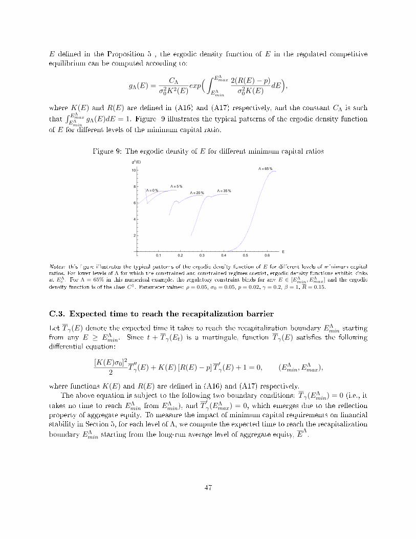
E de�ned in the Proposition 5 , the ergodic density function of E in the regulated competitiveequilibrium can be computed according to:

gΛ(E) =CΛ

σ20K

2(E)exp(∫ EΛ

max

EΛmin

2(R(E)− p)σ2

0K(E)dE),

where K(E) and R(E) are de�ned in (A16) and (A17) respectively, and the constant CΛ is such

that∫ EΛ

max

EΛmin

gΛ(E)dE = 1. Figure 9 illustrates the typical patterns of the ergodic density function

of E for di�erent levels of the minimum capital ratio.

Figure 9: The ergodic density of E for di�erent minimum capital ratios

0.1 0.2 0.3 0.4 0.5 0.6E

2

4

6

8

10

gΛ(E)

Λ = 0%Λ = 5%

Λ = 35%Λ = 20%

Λ = 65%

Notes: this �gure illustrates the typical patterns of the ergodic density function of E for di�erent levels of minimum capitalratios. For lower levels of Λ for which the constrained and constrained regimes coexist, ergodic density functions exhibit kinksat EΛ

c . For Λ = 65% in this numerical example, the regulatory constraint binds for any E ∈ [EΛmin, E

Λmax] and the ergodic

density function is of the class C1. Parameter values: ρ = 0.05, σ0 = 0.05, p = 0.02, γ = 0.2, β = 1, R = 0.15.

C.3. Expected time to reach the recapitalization barrier

Let T γ(E) denote the expected time it takes to reach the recapitalization boundary EΛmin starting

from any E ≥ EΛmin. Since t + T γ(Et) is a martingale, function T γ(E) satis�es the following

di�erential equation:

[K(E)σ0]2

2T′′γ(E) +K(E) [R(E)− p]T ′γ(E) + 1 = 0, (EΛ

min, EΛmax),

where functions K(E) and R(E) are de�ned in (A16) and (A17) respectively.The above equation is subject to the following two boundary conditions: T γ(EΛ

min) = 0 (i.e., it

takes no time to reach EΛmin from EΛ

min), and T′γ(EΛ

max) = 0, which emerges due to the re�ectionproperty of aggregate equity. To measure the impact of minimum capital requirements on �nancialstability in Section 5, for each level of Λ, we compute the expected time to reach the recapitalization

boundary EΛmin starting from the long-run average level of aggregate equity, E

Λ.

47

Appendix D. Competitive equilibrium with r > 0

In the core of the paper we characterized the competitive equilibrium for the particular caser = 0. In this Appendix we solve for the competitive equilibrium for r > 0, focusing on thecontinuous-time framework. When r > 0, the dynamics of equity of an individual bank is given by:

det = retdt+ kt[(R(Et)− p− r)dt − σ0dZt]− dδt + dit. (D1)

The aggregate equity of the banking sector evolves according to:

dEt = [rEt +K(Et)(R(Et)− p− r)]dt− σ0K(Et)dZt − d∆t + dIt. (D2)

Solving the shareholders' maximization problem in the same way as we did in the proof ofProposition 2 and allowing for k > 0 yields us two equations:

u′(E)

u(E)= −R(E)− p− r

σ20K(E)

, (D3)

(ρ− r)u(E) = [rE +K(E)(R(E)− p− r)]u′(E) +σ2

0K2(E)

2u′′(E). (D4)

Using (D3) to compute u′′(E) and substituting it together with u′(E) into (D4) (while takinginto account the equilibrium condition K(E) = L[R(E)]), enables us to express R′(E):

R′(E) = − 1

σ20

2(ρ− r)σ20 + (R(E)− p− r)2 + 2(R(E)− p− r)rE/L[R(E)]

L[R(E)]− (R(E)− p− r)L′[R(E)]. (D5)

Applying the same arguments as in the setting with r = 0, we can show that Emin = 0 andRmin = r + p. The boundary Rmax can be computed numerically by solving equation∫ Rmax

pE′(R)

(R− p− r)σ2

0L(R)dR = log(1 + γ), (D6)

where E′(R) = 1/R′(E).Note that the left-hand side of the above expression is increasing in Rmax. Hence, there exists

a unique solution to (D6), which guarantees the uniqueness of the equilibrium.The typical patterns of the equilibrium loan rate R(E) and net deposits D −M(E) emerging

for di�erent values of r are reported in Figure 10. The following remarks are in order concerningthese numerical results. First, higher r drives up the loan rate, yet, in a non-linear way. Second,as higher R(E) triggers reductions in lending and thus reduces the overall exposure of the bankingsector to aggregate risk, the target level of aggregate capitalization (Emax) declines when r increases.Thus, the interest rate on deposits can be viewed as an additional regulatory instrument of keepingcontrol over aggregate lending and thus �nancial stability. Finally, under assumption that λ(.) is adecreasing function of its argument, condition λ′(D) = ρ − r implies that the aggregate volume ofdeposits increases with r. Thus, aggregate reserves given by M(E) = D −K(E) + E also increasewith r.

48

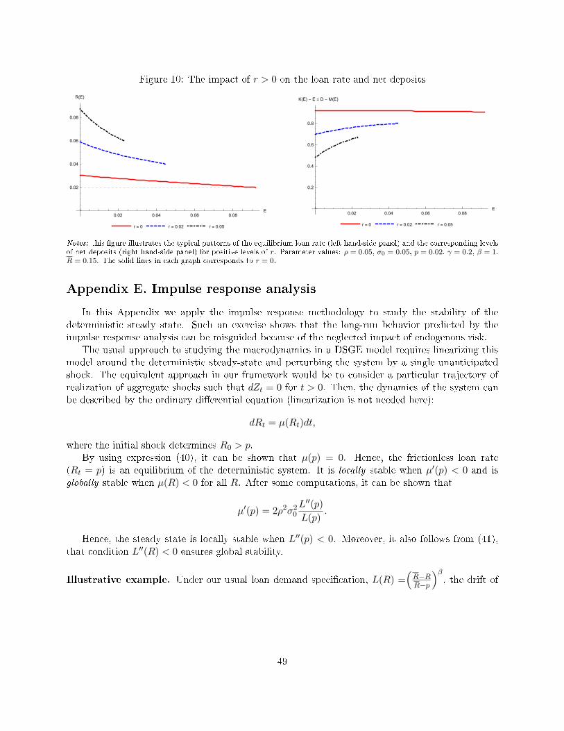
Figure 10: The impact of r > 0 on the loan rate and net deposits

0.02 0.04 0.06 0.08E

0.02

0.04

0.06

0.08

R(E)

r = 0 r = 0.02 r = 0.05

0.02 0.04 0.06 0.08E

0.2

0.4

0.6

0.8

K(E) - E = D - M(E)

r = 0 r = 0.02 r = 0.05

Notes: this �gure illustrates the typical patterns of the equilibrium loan rate (left hand-side panel) and the corresponding levelsof net deposits (right hand-side panel) for positive levels of r. Parameter values: ρ = 0.05, σ0 = 0.05, p = 0.02, γ = 0.2, β = 1,R = 0.15. The solid lines in each graph corresponds to r = 0.

Appendix E. Impulse response analysis

In this Appendix we apply the impulse response methodology to study the stability of thedeterministic steady state. Such an exercise shows that the long-run behavior predicted by theimpulse response analysis can be misguided because of the neglected impact of endogenous risk.

The usual approach to studying the macrodynamics in a DSGE model requires linearizing thismodel around the deterministic steady-state and perturbing the system by a single unanticipatedshock. The equivalent approach in our framework would be to consider a particular trajectory ofrealization of aggregate shocks such that dZt = 0 for t > 0. Then, the dynamics of the system canbe described by the ordinary di�erential equation (linearization is not needed here):

dRt = µ(Rt)dt,

where the initial shock determines R0 > p.By using expression (40), it can be shown that µ(p) = 0. Hence, the frictionless loan rate

(Rt = p) is an equilibrium of the deterministic system. It is locally stable when µ′(p) < 0 and isglobally stable when µ(R) < 0 for all R. After some computations, it can be shown that

µ′(p) = 2ρ2σ20

L′′(p)

L(p).

Hence, the steady state is locally stable when L′′(p) < 0. Moreover, it also follows from (41),that condition L′′(R) < 0 ensures global stability.

Illustrative example. Under our usual loan demand speci�cation, L(R) =(R−RR−p

)β, the drift of

49

the loan rate is given by54

µ(R) = σ(R)β(R− p)Q(R)

2σ0[R+ (β − 1)R− βp]2, (E1)

where Q(R) is a quadratic polynomial:

Q(R) = (1− β)((R− p)2 − 2ρσ20)− 2(R− p)(R− p). (E2)

Given the above speci�cation, it can easily be shown that, when β < 1 (which is equivalent toL′′(R) < 0), µ′(p) < 0 and µ(R) < 0 in the entire interval [p,R]. Thus, the steady state is locallyand globally stable. By contrast, when β > 1 (which is equivalent to L′′(R) > 0), the steady stateis locally unstable, i.e., µ′(p) > 0. Moreover, when the recapitalization cost γ is not too small, thereexists a unique R∗ ∈ (p,R) such that µ(R) is positive in the region (0, R∗) and negative in theregion (R∗, R).

While the outcomes of the impulse response analysis applied to our model might suggest thatthe economy should remain most of the time at the "deterministic" steady state, the analysis of thelong-run behavior of the economy conducted in Section 4.2 shows that it is actually never the casebecause of the signi�cant impact of endogenous risk.

Appendix F. Time-varying �nancing conditions

In the core of the paper we have considered the setting in which the re�nancing cost γ wasconstant over time. In this section we extend the basic model to time-varying �nancing conditions.Assume that the cost of issuing new equity depends on a macroeconomic state that can be Goodor Bad, with the respective costs of recapitalization γG and γB, such that γB > γG. Let ψB denotethe intensity of transition from the Good to the Bad state and ψG denote the intensity of transitionfrom the Bad to the Good state.

Note that the homogeneity property of the individual decision problem is still preserved, so wecan again work directly with the market-to-book value of banks. To ensure that the maximizationproblem of bank shareholders has a non-degenerate solution, the market-to-book value must satisfythe system of simultaneous equations:

ρuG(E) =[KG(E)σ0]2

2u′′G(E) +KG(E) [RG(E)− p]u′G(E)− ψB [uG(E)− uB(E)] , E ∈ (EGmin, E

Gmax)

(F1)

ρuB(E) =[KB(E)σ0]2

2u′′B(E) +KB(E) [RB(E)− p]u′B(E)− ψG [uB(E)− uG(E)] , E ∈ (EBmin, E

Bmax)

(F2)

54Endogenous volatility σ(R) is given by:

σ(R) =

[2ρσ2

0 + (R− p)2]

(R−R)

σ0[R+ (β − 1)R− βp].

50

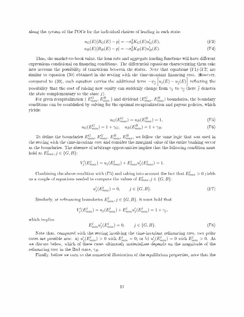
along the system of the FOCs for the individual choices of lending in each state:

uG(E)[RG(E)− p] = −σ20KG(E)u′G(E), (F3)

uB(E)[RB(E)− p] = −σ20KB(E)u′B(E). (F4)

Thus, the market-to-book value, the loan rate and aggregate lending functions will have di�erentexpressions conditional on �nancing conditions. The di�erential equations characterizing them takeinto account the possibility of transitions between the states. Note that equations (F1)-(F2) aresimilar to equation (30) obtained in the setting with the time-invariant �nancing cost. However,

compared to (30), each equation carries the additional term −ψj[uj(E)− uj(E)

]re�ecting the

possibility that the cost of raising new equity can suddenly change from γj to γj (here j denotesthe state complementary to the state j).

For given recapitalization ( EGmin, EBmin ) and dividend (EGmax, E

Bmax) boundaries, the boundary

conditions can be established by solving for the optimal recapitalization and payout policies, whichyields:

uG(EGmax) = uB(EBmax) = 1, (F5)

uG(EGmin) = 1 + γG, uB(EBmin) = 1 + γB. (F6)

To de�ne the boundaries EGmin, EGmax, E

Bmin, E

Bmax, we follow the same logic that was used in

the setting with the time-invariant cost and consider the marginal value of the entire banking sectorat the boundaries. The absence of arbitrage opportunities implies that the following condition musthold at Ejmax, j ∈ {G,B}:

V ′j (Ejmax) = uj(Ejmax) + Ejmaxu

′j(E

jmax) = 1.

Combining the above condition with (F5) and taking into account the fact that Ejmax > 0 yieldsus a couple of equations needed to compute the values of Ejmax, j ∈ {G,B}:

u′j(Ejmax) = 0, j ∈ {G,B}. (F7)

Similarly, at re�nancing boundaries Ejmin, j ∈ {G,B}, it must hold that

V ′j (Ejmin) = uj(Ejmin) + Ejminu

′j(E

jmin) = 1 + γj ,

which impliesEjminu

′j(E

jmin) = 0, j ∈ {G,B}. (F8)

Note that, compared with the setting involving the time-invariant re�nancing cost, two polarcases are possible now: a) u′j(E

jmin) > 0 with Ejmin = 0; or b) u′j(E

jmin) = 0 with Ejmin > 0. As

we discuss below, which of these cases ultimately materializes depends on the magnitude of there�nancing cost in the Bad state, γB.

Finally, before we turn to the numerical illustration of the equilibrium properties, note that the

51

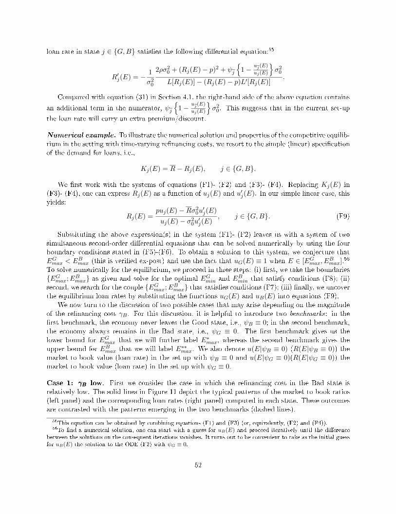
loan rate in state j ∈ {G,B} satis�es the following di�erential equation:55

R′j(E) = − 1

σ20

2ρσ20 + (Rj(E)− p)2 + ψj

{1− uj(E)

uj(E)

}σ2

0

L[Rj(E)]− (Rj(E)− p)L′[Rj(E)].

Compared with equation (31) in Section 4.1, the right-hand side of the above equation contains

an additional term in the numerator, ψj

{1− uj(E)

uj(E)

}σ2

0. This suggests that in the current set-up

the loan rate will carry an extra premium/discount.

Numerical example. To illustrate the numerical solution and properties of the competitive equilib-rium in the setting with time-varying re�nancing costs, we resort to the simple (linear) speci�cationof the demand for loans, i.e.,

Kj(E) = R−Rj(E), j ∈ {G,B}.

We �rst work with the systems of equations (F1)- (F2) and (F3)- (F4). Replacing Kj(E) in(F3)- (F4), one can express Rj(E) as a function of uj(E) and u′j(E). In our simple linear case, thisyields:

Rj(E) =puj(E)−Rσ2

0u′j(E)

uj(E)− σ20u′j(E)

, j ∈ {G,B}. (F9)

Substituting the above expression(s) in the system (F1)- (F2) leaves us with a system of twosimultaneous second-order di�erential equations that can be solved numerically by using the fourboundary conditions stated in (F5)-(F6). To obtain a solution to this system, we conjecture thatEGmax < EBmax (this is veri�ed ex-post) and use the fact that uG(E) ≡ 1 when E ∈ [EGmax, E

Bmax].56

To solve numerically for the equilibrium, we proceed in three steps: (i) �rst, we take the boundaries{EGmax;EBmax} as given and solve for the optimal EGmin and EBmin that satisfy conditions (F8); (ii)second, we search for the couple {EGmax;EBmax} that satis�es conditions (F7); (iii) �nally, we uncoverthe equilibrium loan rates by substituting the functions uG(E) and uB(E) into equations (F9).

We now turn to the discussion of two possible cases that may arise depending on the magnitudeof the re�nancing cost γB. For this discussion, it is helpful to introduce two benchmarks: in the�rst benchmark, the economy never leaves the Good state, i.e., ψB ≡ 0; in the second benchmark,the economy always remains in the Bad state, i.e., ψG ≡ 0. The �rst benchmark gives us thelower bound for EGmax that we will further label E∗max, whereas the second benchmark gives theupper bound for EBmax that we will label E∗∗max. We also denote u(E|ψB ≡ 0) (R(E|ψB ≡ 0)) themarket-to-book value (loan rate) in the set-up with ψB ≡ 0 and u(E|ψG ≡ 0)(R(E|ψG ≡ 0)) themarket-to-book value (loan rate) in the set-up with ψG ≡ 0.

Case 1: γBγBγB low. First we consider the case in which the re�nancing cost in the Bad state isrelatively low. The solid lines in Figure 11 depict the typical patterns of the market-to-book ratios(left panel) and the corresponding loan rates (right panel) computed in each state. These outcomesare contrasted with the patterns emerging in the two benchmarks (dashed lines).

55This equation can be obtained by combining equations (F1) and (F3) (or, equivalently, (F2) and (F4)).56To �nd a numerical solution, one can start with a guess for uB(E) and proceed iteratively until the di�erence

between the solutions on the consequent iterations vanishes. It turns out to be convenient to take as the initial guessfor uB(E) the solution to the ODE (F2) with ψG ≡ 0.

52

Several equilibrium features are worth mentioning at this stage. First, one can note thatEGmin = EBmin = 0, so that banks do not change their recapitalization policies as compared tothose implemented in the benchmark settings. By contrast, EGmax > E∗max and EBmax < E∗∗max,which means that banks will delay the distribution of dividends as compared to the setting in whichthe economy permanently remains in the Good state and will accelerate dividend payments as com-pared to the setting in which the economy is permanently locked in the Bad state. Second, in theGood state, the loan rate carries a �discount� (as compared to its benchmark value obtained forψB ≡ 0) when E is low and an extra �premium� when E is high enough. By contrast, the loanrate in the Bad state carries an extra �premium�(as compared to its benchmark value obtained forψG ≡ 0) for lower level of E and a �discount� when E is high.

Figure 11: Competitive equilibrium with time-varying �nancing costs: γB low

0.002 0.004 0.006 0.008 0.010 0.012E

1.0

1.2

1.4

1.6

1.8

2.0

uG(E), uB(E)

0.002 0.004 0.006 0.008 0.010 0.012E

0.020

0.025

0.030

0.035

0.040

0.045

RG(E), RB(E)

RB(E)

RG(E)

uB(E)uG(E)

u(E|ψG ≡ 0)

u(E|ψB ≡ 0)

R(E|ψB ≡ 0)R(E|ψG ≡ 0)

Parameter values: ρ = 0.05, σ0 = 0.05, p = 0.02, γG = 0.2, γB = 1, ψG = 0.1, ψB = 0.05; L(R) = R − R with R = 0.1.The benchmark payout barriers are: E∗max ≈ 0.007 and E∗∗max ≈ 0.012. The payout barriers in the Good and Bad regimes are:EGmax ≈ 0.008 and EBmax ≈ 0.011.

Case 2: γBγBγB high. We now turn to the setting involving very high re�nancing costs in the Bad state.The properties of the competitive equilibrium emerging in this case are illustrated in Figure 12.The key departure from the previous case pertains to the fact that, for fear of incurring substantialrecapitalization costs if the economy slides in the Bad state, in the Good state banks will raise newequity capital at a strictly positive level of aggregate capitalization, i.e., EGmax > 0. In a dynamicsetting, this phenomenon of �market timing� was �rst identi�ed by Bolton et al. (2013) within apartial-equilibrium liquidity-management model with the stochastically changing �xed cost of equityissuance. The main general-equilibrium implication of this feature in our setting is that the loanrate (and, therefore, the volume of lending) converges to its First-Best level when E → EGmin and�nancing conditions are good (i.e., j = G).

Appendix G. Empirical analysis

This Appendix presents a simple assessment of the consistency of the key predictions of our modelwith the data. As stated in Proposition 1, our model delivers two key predictions: bank loan ratesand the ratio of market-to-book equity are (weakly) decreasing functions of aggregate bank equity.

53

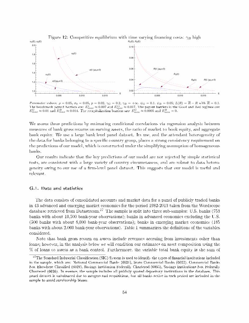
Figure 12: Competitive equilibrium with time-varying �nancing costs: γB high

0.005 0.010 0.015E

1.0

1.2

1.4

1.6

1.8

2.0

uG(E), uB(E)

0.005 0.010 0.015E

0.02

0.04

0.06

0.08

0.10

RG(E), RB(E)

uG(E)

u(E|ψB ≡ 0)

uB(E)

u(E ψG ≡ 0)

RG(E)

R(E ψB ≡ 0)

RB(E) R(E ψG ≡ 0)

Parameter values: ρ = 0.05, σ0 = 0.05, p = 0.02, γG = 0.2, γB = +∞, ψG = 0.1, ψB = 0.05; L(R) = R − R with R = 0.1.The benchmark payout barriers are: E∗max ≈ 0.007 and E∗∗max ≈ 0.017. The payout barriers in the Good and Bad regimes are:EGmax ≈ 0.01 and EBmax ≈ 0.014. The recapitalization barriers are: EGmin ≈ 0.0005 and EBmin = 0.

We assess these predictions by estimating conditional correlations via regression analysis betweenmeasures of bank gross returns on earning assets, the ratio of market-to-book equity, and aggregatebank equity. We use a large bank-level panel dataset. Its use, and the attendant heterogeneity ofthe data for banks belonging to a speci�c country group, places a strong consistency requirement onthe predictions of our model, which is constructed under the simplifying assumption of homogeneousbanks.

Our results indicate that the key predictions of our model are not rejected by simple statisticaltests, are consistent with a large variety of country circumstances, and are robust to data hetero-geneity owing to our use of a �rm-level panel dataset. This suggests that our model is useful andrelevant.

G.1. Data and statistics

The data consists of consolidated accounts and market data for a panel of publicly traded banksin 43 advanced and emerging market economies for the period 1982-2013 taken from the Wordscopedatabase retrieved from Datastream.57 The sample is split into three sub-samples: U.S. banks (753banks with about 10,500 bank-year observations); banks in advanced economies excluding the U.S.(500 banks with about 8,000 bank-year observations); banks in emerging market economies (185banks with about 2,000 bank-year observations). Table 1 summarizes the de�nitions of the variablesconsidered.

Note that bank gross return on assets include revenues accruing from investments other thanloans; however, in the analysis below we will condition our estimates on asset composition using the% of loans to assets as a bank control. Furthermore, the variable total bank equity is the sum of

57The Standard Industrial Classi�cation (SIC) System is used to identify the types of �nancial institutions includedin the sample, which are: National Commercial Banks (6021), State Commercial Banks (6022), Commercial BanksNot Elsewhere Classi�ed (6029), Savings Institution Federally Chartered (6035), Savings Institutions Not FederallyChartered (6036). In essence, the sample includes all publicly quoted depository institutions in the database. Thispanel dataset is unbalanced due to mergers and acquisitions, but all banks active in each period are included in thesample to avoid survivorship biases.

54

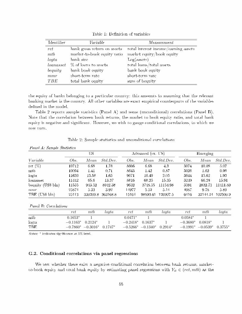
Table 1: De�nition of variables

Identi�er Variable Measurement

ret bank gross return on assets total interest income/earning assetsmtb market-to-book equity ratio market equity/book equitylogta bank size Log(assets)loanasset % of loans to assets total loans/total assetsbequity bank book equity bank book equitymmr short-term rate short-term rateTBE total bank equity sum of bequity

the equity of banks belonging to a particular country: this amounts to assuming that the relevantbanking market is the country. All other variables are exact empirical counterparts of the variablesde�ned in the model.

Table 2 reports sample statistics (Panel A) and some (unconditional) correlations (Panel B).Note that the correlation between bank returns, the market-to-book equity ratio, and total bankequity is negative and signi�cant. However, we wish to gauge conditional correlations, to which wenow turn.

Table 2: Sample statistics and unconditional correlations

Panel A: Sample Statistics

US Advanced (ex. US) Emerging

V ariable Obs. Mean Std.Dev. Obs. Mean Std.Dev. Obs. Mean Std.Dev.

ret (%) 10712 6.68 1.78 8606 6.68 4.3 3074 10.08 5.07mtb 10094 1.41 0.71 8645 1.42 0.87 3028 1.62 0.98logta 11630 13.58 1.65 9671 16.49 2.05 3644 15.62 1.93loanasset 11442 65.6 13.37 8816 68.25 15.35 3240 66.28 15.91bequity (US$ bln) 11555 943.52 8942.38 9632 3748.55 11154.98 3591 2832.71 11411.89mmr 25874 5.33 3.92 14977 5.52 5.14 4987 9.78 5.89TBE (US$ bln) 25113 330209.8 363168.8 15164 98893.61 126907.5 6416 32144.24 102500.9

Panel B: Correlations

ret mtb logta ret mtb logta ret mtb logta

mtb 0.1653∗ 1 0.0471∗ 1 0.0584∗ 1logta −0.1163∗ 0.2124∗ 1 −0.2418∗ 0.1637∗ 1 −0.3680∗ 0.0818∗ 1TBE −0.7860∗ −0.3016∗ 0.1747∗ −0.5266∗ −0.1340∗ 0.2914∗ −0.1991∗ −0.0539∗ 0.3755∗

Notes: ∗ indicates signi�cance at 5% level.

G.2. Conditional correlations via panel regressions

We test whether there exist a negative conditional correlation between bank returns, market-to-book equity and total bank equity by estimating panel regressions with Yit ∈ (ret,mtb) as the

55

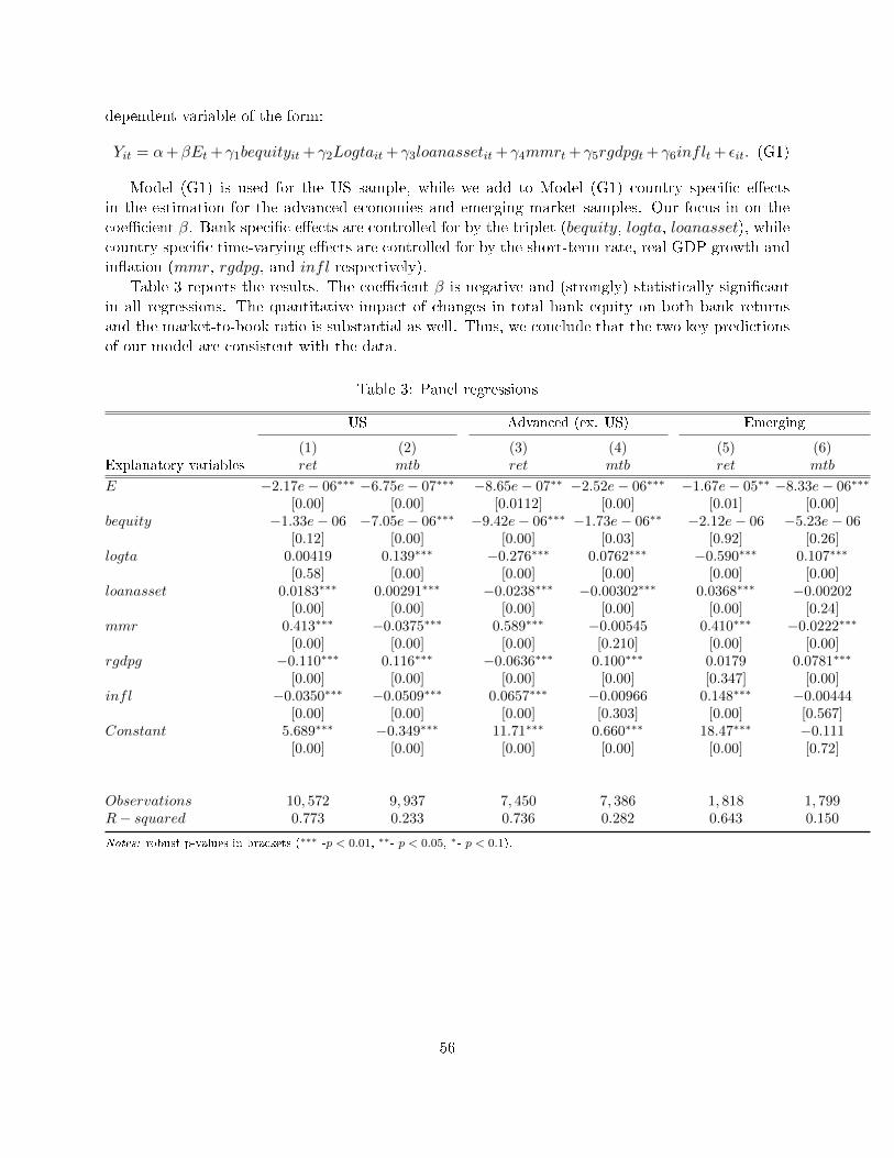
dependent variable of the form:

Yit = α+βEt + γ1bequityit + γ2Logtait + γ3loanassetit + γ4mmrt + γ5rgdpgt + γ6inflt + εit. (G1)

Model (G1) is used for the US sample, while we add to Model (G1) country speci�c e�ectsin the estimation for the advanced economies and emerging market samples. Our focus in on thecoe�cient β. Bank speci�c e�ects are controlled for by the triplet (bequity, logta, loanasset), whilecountry speci�c time-varying e�ects are controlled for by the short-term rate, real GDP growth andin�ation (mmr, rgdpg, and infl respectively).

Table 3 reports the results. The coe�cient β is negative and (strongly) statistically signi�cantin all regressions. The quantitative impact of changes in total bank equity on both bank returnsand the market-to-book ratio is substantial as well. Thus, we conclude that the two key predictionsof our model are consistent with the data.

Table 3: Panel regressions

US Advanced (ex. US) Emerging

(1) (2) (3) (4) (5) (6)Explanatory variables ret mtb ret mtb ret mtb

E −2.17e− 06∗∗∗ −6.75e− 07∗∗∗ −8.65e− 07∗∗ −2.52e− 06∗∗∗ −1.67e− 05∗∗ −8.33e− 06∗∗∗

[0.00] [0.00] [0.0112] [0.00] [0.01] [0.00]bequity −1.33e− 06 −7.05e− 06∗∗∗ −9.42e− 06∗∗∗ −1.73e− 06∗∗ −2.12e− 06 −5.23e− 06

[0.12] [0.00] [0.00] [0.03] [0.92] [0.26]logta 0.00419 0.139∗∗∗ −0.276∗∗∗ 0.0762∗∗∗ −0.590∗∗∗ 0.107∗∗∗

[0.58] [0.00] [0.00] [0.00] [0.00] [0.00]loanasset 0.0183∗∗∗ 0.00291∗∗∗ −0.0238∗∗∗ −0.00302∗∗∗ 0.0368∗∗∗ −0.00202

[0.00] [0.00] [0.00] [0.00] [0.00] [0.24]mmr 0.413∗∗∗ −0.0375∗∗∗ 0.589∗∗∗ −0.00545 0.410∗∗∗ −0.0222∗∗∗

[0.00] [0.00] [0.00] [0.210] [0.00] [0.00]rgdpg −0.110∗∗∗ 0.116∗∗∗ −0.0636∗∗∗ 0.100∗∗∗ 0.0179 0.0781∗∗∗

[0.00] [0.00] [0.00] [0.00] [0.347] [0.00]infl −0.0350∗∗∗ −0.0509∗∗∗ 0.0657∗∗∗ −0.00966 0.148∗∗∗ −0.00444

[0.00] [0.00] [0.00] [0.303] [0.00] [0.567]Constant 5.689∗∗∗ −0.349∗∗∗ 11.71∗∗∗ 0.660∗∗∗ 18.47∗∗∗ −0.111

[0.00] [0.00] [0.00] [0.00] [0.00] [0.72]

Observations 10, 572 9, 937 7, 450 7, 386 1, 818 1, 799R− squared 0.773 0.233 0.736 0.282 0.643 0.150

Notes: robust p-values in brackets (∗∗∗ -p < 0.01, ∗∗- p < 0.05, ∗- p < 0.1).

56

References

Admati, A., DeMarzo, P., Hellwig, M., and P. P�eiderer, 2011. Fallacies, Irrelevant Facts, andMyths in the Discussion of Capital Regulation: Why Bank Equity is Not Expensive. Mimeo.

Admati, A., and M. Hellwig, 2013. The Bankers' New Clothes: What's Wrong with Banking andWhat to Do about It. Princeton University Press.

Adrian, T., and H. Shin, 2010. Liquidity and leverage. Journal of Financial Intermediation 19,418 - 437.

Aikman, D., Haldane, A. G. and B. D. Nelson, 2014. Curbing the Credit Cycle. The EconomicJournal. doi: 10.1111/ecoj.12113.

Baron, M., 2015. Countercyclical Bank Equity Issuance. Princeton University, Working Paper.

Becker, B., and V. Ivashina, 2014. Cyclicality of credit supply: Firm level evidence. Journal ofMonetary Economics 62, 76-93.

Begenau, J., 2015. Capital Requirements, Risk Choice, and Liquidity Provision in a BusinessCycle Model. Working Paper.

Berrospide, J. M. and R. M. Edge, 2010. The E�ects of Bank Capital on Lending: What Do WeKnow, and What Does it Mean? International Journal of Central Banking 6, 5-54.

Bernanke, B., Gertler, M., and S. Gilchrist, 1996. The Financial accelerator and the �ight toquality. The Review of Economics and Statistics 78, 1 - 15.

Biais, B., Mariotti, T., Plantin, G. and J.-Ch. Rochet, 2007. Dynamic security design: convergenceto continuous time and asset pricing implications. The Review of Economic Studies 74, 345 -390.

Bolton, P., H. Chen, and N. Wang, 2011. A Uni�ed Theory of Tobin's q, Corporate Investment,Financing, and Risk Management. Journal of Finance, 66, 1545 - 1578.

Bolton, P., H. Chen, and N. Wang, 2013. Market Timing, Investment, and Risk Management.Journal of Financial Economics 109, 40 - 62.

Bridges, J., Gregory, D., Nielsen, M., Pezzini, S., Radia, A. and M. Spaltro, 2014. The impact ofcapital requirements on bank lending. Bank of England Working Paper n◦486.

Brunnermeier, M. K. and Y. Sannikov, 2014. A Macroeconomic Model with a Financial Sector.American Economic Review 104, 379 - 421.

Brunnermeier, M. K. and Y. Sannikov, 2015. International Credit Flows and Pecuniary External-ities. American Economic Journal: Macroeconomics 7, 297 - 338.

DeAngelo, H., and R. M. Stulz, 2014. Why High Leverage is Optimal for Banks. Fisher Collegeof Business WP 2013-03-08.

Décamps, J.P., T. Mariotti, J.C. Rochet, and S. Villeneuve, 2011. Free Cash Flow, Issuance Costs,and Stock Prices. Journal of Finance, 66, 1501-1544.

57

Dell'Ariccia, G., and R. Marquez, 2006. Lending Booms and Lending Standards. Journal of Fi-nance 61, 2511 - 2546.

De Nicolò, G., A. Gamba, and M. Lucchetta, 2014. Microprudential Regulation in a DynamicModel of Banking. Review of Financial Studies 27, 2097 - 2138.

Diamond, D., and P. Dybvig, 1983. Bank runs, deposit insurance, and liquidity. Journal of PoliticalEconomy 99, 689-721.

Diamond, D., and R. Rajan, 2000. A theory of bank capital. Journal of Finance 55, 2431-2465.

Di Tella, S., 2014. Uncertainty Shocks and Balance Sheet Recessions. Working Paper, StanfordGSB.

Freixas, X. and J.-Ch. Rochet, 2008. Microeconomics of Banking, MIT Press.

Gennaioli, N., Schleifer, A., and R.W. Vishny, 2013. A Model of Shadow Banking. Journal ofFinance 68, 1331 - 1363.

Gornall, W., and I. A., Strebulaev, 2015. Financing as a Supply Chain: The Capital Structure ofBanks and Borrowers. Working Paper.

Gorton, G., 2010. Slapped by the Invisible Hand: The Panic of 2007. Oxford University Press,Oxford, UK.

Gorton, G., Pennacchi, G., 1990. Financial intermediaries and liquidity creation. Journal of Fi-nance 45, 49-72.

He, Z. and A. Krishnamurthy, 2012. A Model of Capital and Crises. Review of Economic Studies79, 735-77.

He, Z. and A. Krishnamurthy, 2013. Intermediary Asset Pricing. American Economic Review 103,732 - 770.

Hellwig, M., 2015. Liquidity provision and Equity Funding of Banks. Discussion Paper, MaxPlanck Institute.

Hennessy, C. A. and T. M. Whited, 2007. How costly is external �nancing: Evidence from astructural estimation. Journal of Finance 62, 1705 - 1745.

Holmström, B., Tirole, J., 1997. Financial intermediation, loanable funds, and the real sector.Quarterly Journal of Economics 112, 663-691.

Holmström, B., Tirole, J., 1998. Private and public supply of liquidity. Journal of Political Econ-omy 196, 1-40.

Hugonnier, J. N., and E. Morellec, 2015. Bank Capital, Liquid Reserves, and Insolvency Risk.Working Paper, Swiss Finance Institute and EPFL.

Institute for International Finance, 2010. Interim Report on the Cumulative Impact on the GlobalEconomy of Proposed Changes in Banking Regulatory Framework, Washington, DC: Institute forInternational Finance.

58

Isohätälä, J., Milne A., and D. Robertson, 2014. The net worth trap: investment and outputdynamics in the presence of �nancing constraints. Bank of Finland Research Discussion PaperNo. 26/2014.

Isohätälä, J., Klimenko, N., and A. Milne, 2015. Post-crisis macro �nancial modelling: contin-uous time approaches. Forthcoming in "Handbook of post crisis nancial modelling", PalgraveMacMillan.

Jeanblanc, M., and A. N. Shiryaev, 1995. Optimization of the �ow of dividends. Russian Mathe-matical Surveys 50, 257 - 277.

Jiménez, G., and J. Saurina, 2006. Credit Cycles, Credit Risk, and Prudential Regulation. Inter-national Journal of Central Banking 2, 65-98.

Klimenko, N., Pfeil, S., and J.-Ch. Rochet, 2015. The Apples of Wrath: A Lucas Model withFinancial Frictions. Working Paper.

Kiyotaki, N. and J. Moore, 1997. Credit Cycles. Journal of Political Economy 105, 211 - 48.

Lee, I., S. Lochhead, J. Ritter, and Q. Zhao, 1996. The Costs of Raising Capital. Journal ofFinancial Research 19 , 59-74.

Lucas, R., 1978. Asset Prices in an Exchange Economy. Econometrica 46, 1429 - 1445.

Martinez-Miera, D., and R. Repullo, 2010. Does Competition Reduce the Risk of Bank Failure?Review of Financial Studies 23, 3638 -3664.

Martinez-Miera, D., and J. Suarez, 2014. A Macroeconomic Model of Endogenous Systemic RiskTaking. Mimeo, CEMFI.

Meh, C., and K. Moran, 2010. The role of bank capital in the propagation of shocks. Journal ofEconomic Dynamics and Control 34, 555 - 576.

Nguyên, T., 2014. Bank Capital Requirements: A quantitative Analysis. Working Paper.

Pandit, V., 2010. We must rethink Basel, or growth will su�er. Financial Times, 10 November.

Phelan, G., 2015. Financial Intermediation, Leverage, and Macroeconomic Instability. Forthcom-ing in American Economic Journal: Macroeconomics.

Stein, J., 2012. Monetary Policy as Financial Stability Regulation. Quarterly Journal of Economics127, 57-95.

TheCityUK report, October 2013. Alternative �nance for SMEs and mid-market companies.

Van den Heuvel, S. J., 2008. The welfare cost of bank capital requirements. Journal of MonetaryEconomics 55, 298 - 320.

59