Heterogeneous Bank Lending Responses to Monetary Policy:

New Evidence from a Real-time Identification

John C. Bluedorn∗ ‡

j.bluedorn@soton.ac.uk

Christopher Bowdler† ‡

christopher.bowdler@economics.ox.ac.uk

Christoffer Koch† ‡

christoffer.koch@economics.ox.ac.uk

August 2009

Abstract: Heterogeneity in bank responses to monetary policy is consistent with an aggregatelending channel. However, estimates of bank responses are typically obtained using realizedfederal funds rate changes, which are endogenous to expected, macroeconomic fundamentals.As such, estimated heterogeneity can arise from expected fundamentals. Using an exogenouspolicy measure identified from narratives on FOMC intentions and real-time forecasts, we findgreater heterogeneity in responses. There is a much stronger monetary policy transmission tosmaller banks. The shielding of lending amongst holding companies is larger using the exogenousmeasure. Unlike previous research, we find that holdings of securities amplify exogenous policytransmission, while equity capital negates it. The results highlight the importance of controllingfor policy endogeneity in future studies of bank lending behavior.

JEL Classification: E44, E50, G21Keywords: monetary transmission, lending channel, monetary policy identification, banking

∗Economics Division, School of Social Sciences, University of Southampton, Southampton SO17 1BJ, UK.†Department of Economics, University of Oxford, Manor Road Building, Manor Road, Oxford OX1 3UQ, UK.‡We thank Adam Ashcraft for providing his bank-level dataset and seminar participants at the University

of Southampton, Magyar Nemzeti Bank (Hungarian Central Bank), Saıd Business School, Oxford, and LehmanBrothers, London, for comments on earlier versions of this paper.

1 Introduction

The role of the banking sector in the transmission of monetary policy has been studied in

great detail in both the theoretical and applied literature. According to the theory of the

lending channel, contractionary open market operations reduce banking sector reserves and

deposits, forcing a reduction in lending volumes because banks are constrained in their ability

to substitute lost deposits with alternative sources of finance. In practice, this mechanism may

be reinforced by a broader credit channel, whereby tight policy reduces borrower collateral and

induces banks to raise the premium on loans relative to the competitive cost of funds (the

external finance premium). Propagation of monetary policy via these loan supply channels is

different from textbook treatments of monetary transmission which emphasize the sensitivity

of aggregate expenditure to interest rate movements.1

Following the work of Kashyap and Stein (2000), a number of empirical studies have explored

the heterogeneity in bank lending responses to monetary policy. To the extent that financing

constraints vary with banks’ access to liquidity and collateral, the existence of a lending channel

implies that loan responses to policy are a function of observable bank characteristics related to

such access. Kashyap and Stein show that banks with relatively large and liquid asset bases are

better able to shield their lending growth during periods of tight monetary policy. The same

phenomenon has been documented for banks with relatively high equity capital-to-assets ratios

(Kishan and Opiela, 2000), banks whose loan books are readily securitized (Loutskina, 2005),

banks affiliated to a holding company (Ashcraft, 2006), and banks that can raise funds from

international operations (Cetorelli and Goldberg, 2008).

A fundamental issue addressed in each of these papers is whether heterogeneity linked to

a specific characteristic can be interpreted as a loan supply effect (as in the narrow and broad

lending channels), rather than an amalgam of possible loan supply and loan demand effects.

A large amount of evidence for homogeneous loan demand conditional upon one or more bank

characteristics has been provided.2 With homogenous loan demands, any heterogeneity in

lending responses across the conditioning bank characteristics is consistent with the existence

of a bank lending channel affecting loan supply.

By contrast, much less attention has been devoted to the question of what measure of

1See Bernanke and Gertler (1995) for a review of the different elements of the transmission mechanism.2See Ashcraft (2006) for a discussion of this evidence.

1

monetary policy is appropriate for the assessment of bank lending behavior. Most papers use

the change in the effective (realized) federal funds rate to capture monetary policy, reflecting

the fact that the Federal Open Market Committee (FOMC) has targeted the federal funds rate

for much of the last 30 years.3 While federal funds rate changes initiated by the FOMC are

surely exogenous to the circumstances facing any single bank, the factors to which policymakers

respond (e.g., expected output growth and inflation) are potential determinants of individual

bank lending, through both loan demand and loan supply effects. This raises the possibility

that lending responses to federal funds rate changes confound the effects of monetary policy

and other lending market drivers. Furthermore, if the strength of any effects from confounding

variables is related to bank characteristics, the heterogeneity in lending responses to monetary

policy will not be correctly estimated.

Motivated by these possibilities, we evaluate the heterogeneity in bank lending responses

to federal funds rate changes that are plausibly exogenous to expected output growth and

inflation. The identification of this policy component builds upon work by Romer and Romer

(2004), who combined narrative evidence on Federal Reserve intentions and the Greenbook

forecasts produced by Federal Reserve staff in order to control for endogenous policy changes.

Bank lending responses to the identified policy measure are compared with lending responses

estimated from realized federal funds rate changes that have been the focus of most previous

research.

Our results indicate five important differences in bank lending responses to exogenous and

endogenous components of monetary policy. First, one year after an exogenous monetary con-

traction, the reduction in lending growth at the average bank which is not part of a holding

company is up to twice that from a rise in the realized federal funds rate. Second, the amount by

which a bank can shield its lending growth from a monetary policy contraction, either through

accessing a large asset base or drawing on funds from affiliates in a holding company, is 1.5 times

larger when estimated purely in response to identified, exogenous monetary policy. Third, the

share of bank assets held as securities mitigates the lending response to a realized federal funds

rate increase, but amplifies the lending contraction to an exogenous federal funds rate increase.

In contrast, the ratio of equity capital-to-assets shields lending growth from an exogenous mon-

3Alternative monetary policy measures which have been used in the literature on bank lending include thosedue to Boschen and Mills (1991, 1995), Strongin (1995), and Bernanke and Mihov (1998). See section 2 forfurther discussion.

2

etary tightening, but is only weakly correlated with lending responses to realized federal funds

rate increases.

We offer explanations for these findings in terms of the endogeneity of monetary policy. They

provide a new perspective on the measurement of balance sheet liquidity and the consequences

of shifts in balance sheet composition for the strength of monetary policy propagation. Our

fourth finding qualifies the results on balance sheet composition. Following the introduction

of the source of strength doctrine for bank holding companies in 1987, the effects of asset

composition on lending responses to monetary policy occur only among banks that are not part

of a holding company. Affiliated banks appear to be able to smooth lending in the face of

monetary policy shocks using the internal capital markets of the holding company, such that

balance sheet composition does not affect lending responses to monetary policy. Fifth and

lastly, banks that do a larger proportion of business in the residential sector contract lending by

a smaller amount following an exogenous policy tightening. This is consistent with better access

to the finance needed to sustain such loans, as might arise with securitization (Loutskina, 2005).

In contrast, following changes in the realized federal funds rate, this effect is much smaller and

only marginally significant.

To place our paper in context, it is important to consider how potential biases from con-

founding monetary policy with other loan demand and loan supply determinants have been

handled in previous research. Each of the papers discussed earlier directly controls for output

growth, inflation, or both, in their empirical models of lending growth. To the extent that

such variables effectively capture the sources of endogenous monetary policy, their inclusion in

a lending growth regression accounts for extraneous loan demand and loan supply shifters, such

that the structural effects of policy can be identified. Under the assumption that loan demand

does not vary with the characteristic, heterogeneity in these structural effects is then measured

via interactions with bank characteristics.

The starting point for our paper is that current output growth and inflation are not the only

sources of endogenous policy – a forward-looking policymaker who desires to minimize cyclical

fluctuations will also respond to forecasts for its objective variables. If these forecasts correlate

with private sector expectations for growth and inflation, loan demand and loan supply may

fluctuate in a manner that is systematically related to observable bank characteristics. Our

3

results highlight instances in which this appears to be the case. In light of these findings, we

argue that future studies of bank lending behavior should take into account the forward-looking

component of endogenous monetary policy.

The remainder of the paper is structured as follows. In section 2, we explain how endogenous

monetary policy movements may induce biased estimates of lending responses to monetary

policy. Motivated by these possibilities, in section 3 we outline an identification strategy for

exogenous monetary policy. We then discuss the bank-level econometric framework and data

that we use to compare lending responses to identified policy changes with lending responses

to realized changes in the federal funds rate. In section 4, we present our core results. We

continue in section 5 with a consideration of their robustness to changes in estimation and data

definitions. Finally, we conclude in section 6 with a summary and a discussion of the importance

of monetary policy identification for future research concerning bank lending behavior.

2 Bank lending and monetary policy

How might endogenous monetary policy contaminate estimates of the lending channel? Here, we

outline the potential biases affecting the estimates in the literature that rely upon the effective

federal funds rate to measure monetary policy. In each of the cases discussed, the underlying

idea is that expectations over output growth and inflation determine both policy and bank

lending choices. These effects are not captured in the standard lending growth regression.

Consequently, there is an omitted variable problem that affects the estimated response of bank

lending to federal funds rate changes. Moreover, our discussion covers lending responses that

are conditional upon bank characteristics, which have received considerable attention in recent

research. We argue that estimates of these cross effects are also affected by the endogeneity of

monetary policy. In light of the possible effects described, we compare bank lending responses

to exogenous monetary policy changes (described in section 3.1) and to the realized monetary

policy changes that have been used in previous research.

Studies of bank lending responses to monetary policy typically estimate regressions of the

form:

∆Li,t

(1×1)

= α + β Mt(1×1)

+ X ′i,t

(1×J)

γ(J×1)

+ X ′i,tMt

(1×J)

δ(J×1)

+ Z ′i,t

(1×K)

φ(K×1)

+ εi,t (1)

4

where i indexes banks, t indexes time, ∆L denotes the change (t minus t − 1) in the natural

logarithm of total loans measured at current prices, M is a monetary policy measure, X is a

vector of J bank-specific characteristics, Z is a vector of K control variables, and ε is a mean-

zero error term. All other Greek letters denote parameters. In practice, bank lending regressions

are much richer than equation 1, typically including autoregressive terms and dynamics in M

and X. In section 3, we describe a more complex version of model 1 that incorporates these

features. It also will provide the basis for our empirical work. However, the present specification

is sufficient to illustrate the arguments that we develop in this section.4

As noted in the introduction, the vector X comprises bank characteristics that capture

access to finance. These might include total bank assets, bank holding company affiliation, an

indicator for whether a bank operates internationally, measures of balance sheet composition

such as equity capital-to-assets and securities-to-assets ratios, and information concerning the

characteristics of the bank loan book (e.g., the ease with which it can be securitized). In the

aftermath of contractionary monetary policy, banks that can access funds from these sources

may shield lending growth from the effects of an erosion of reserves and deposits.

What interpretation can be given to the cross effects (interactions) between monetary policy

and bank characteristics? It is commonly argued that while factors such as bank size and the

bank equity ratio may capture access to funds that matters for loan supply, they also reflect

features of loan demand. For example, large banks may cherry pick customers whose loan

demand is relatively stable, while poorly capitalized banks may be overlooked by safe borrowers

and forced to do business with risky customers whose loan demand is relatively volatile. On

the other hand, Ashcraft (2006) presents evidence that bank holding company affiliation is

less closely linked to the customer mix, and is to be preferred as an indicator for loan supply

conditions. In this paper, we do not add to this debate. Instead, we consider the range of

characteristics that have been studied in the literature. However, throughout our discussion we

are mindful of the interpretations that can be given to cross effects between monetary policy

and individual bank characteristics.

The monetary policy measure M most often employed is the change in the period average

4Alternatives to the single-step regression model have also been considered in the literature. Kashyap andStein (2000) adopt a two-stage procedure, where the cross-sectional sensitivity of lending growth to balancesheet liquidity is estimated in a first stage, and a time series regression relating these cross-sectionally estimatedliquidity constraints to monetary policy is estimated in a second stage. We do not adopt the two-stage approachin this paper.

5

effective federal funds rate, which has been the Federal Reserve’s operating target since at least

1994, and arguably for many episodes since the post-war period.5 Increases in the federal funds

rate target induce leftward shifts of banks’ loan supply schedules via the narrow and broad

lending channels described in the introduction. These raise lending rates and reducing lending

volumes. When the federal funds rate target is increased in response to forecasts of higher

future economic growth and/or inflation, estimation of this relationship is no longer straight-

forward. In such circumstances, any loan supply contraction due to tight monetary policy may

coincide with a rightward shift of loan demand, as consumers borrow against expected future

income and firms invest in response to an improving outlook for profits. The loan demand shift

will attenuate the reduction in lending from a monetary tightening and the β estimated from

equation 1 will not capture the full effect of monetary policy. A similar result may arise via the

effects of expected inflation. In particular, reductions in bank lending from a rise in the federal

funds rate may be muted because the demand for loans in nominal units rises with expected

inflation. As in the example based on expected economic growth, equilibrium lending is subject

to countervailing effects from loan demand and loan supply, such that the β estimated from

equation 1 is attenuated.

The drivers of endogenous monetary policy may also influence equilibrium lending via bank

loan supply curves. The availability of non-deposit finance to banks is likely to vary positively

with expected economic growth. At the start of cyclical upturns, institutional investors (e.g.,

pension funds, sovereign wealth funds) may invest more heavily in equities and loan-backed

securities, at the expense of fixed income assets, given a greater appetite for higher yields and

risk. To the extent that banks use equity issues and the securitization of loans to generate

funding for new lending, loan supply will rise at each level of market interest rates.

Similarly, in models featuring information asymmetries and monitoring costs, loan supply

incorporates an external finance premium that varies positively with lender risk aversion and

5See Meulendyke (1998) for historical evidence on the Federal Reserve’s policy tool choices. Alternative policymeasures due to Boschen and Mills (1991, 1995) and Bernanke and Mihov (1998) have also been employed inthe literature (Kashyap and Stein, 2000). These measures of policy explicitly address possible changes to theinstrument of policy through time, but remain measures of the endogenous stance of policy. As such, we believethat the arguments developed in this section are applicable to them. Loutskina (2005) considers the Strongin(1995) identification of exogenous movements in non-borrowed reserves. While this approach controls for reservedemand shocks, it does not directly control for endogenous policy moves by a forward-looking central bank. Jonasand King (2008) briefly consider the original Romer and Romer (2004) policy measure, which does control forpolicy endogeneity. However, this is used only as a robustness test in a study that focuses on the impact of bankefficiency on lending responses to general federal funds rate movements. The consequences of policy endogeneityfor lending responses are not considered by Jonas and King.

6

negatively with borrower net worth (via a collateral effect) (Bernanke and Gertler, 1989). Ex-

pansion phases of the business cycle are typically associated with increases in lenders’ risk

appetite and agents’ net worth, such that the external finance premium falls and loan supply

expands. We do not emphasize any one of these channels ahead of the others. Instead, we

highlight that when loan supply is affected by any one of them, the response of lending growth

to the federal funds rate will be attenuated – the leftward shift of loan supply from tight policy

is offset by a rightward shift of loan supply via one of the channels described. Furthermore, this

will be the case even when controlling for current economic growth and inflation. The effect

derives from the fact that expected economic conditions may influence monetary policy and loan

supply simultaneously.

2.1 Policy endogeneity and bank characteristics

An important question is whether or not pro-cyclical loan demand and loan supply affect the

cross effects in equation 1 that measure heterogeneity in bank lending responses. As discussed

in the introduction, these are the terms that proxy the bank-level financial constraints that

underpin the aggregate lending channel of monetary policy. Even if loan demands and supplies

are affected identically across banks by expected macroeconomic conditions, the estimates of

any heterogeneity in bank responses to the exogenous component of monetary policy will be

attenuated. In this case, FF would implicitly introduce measurement error for policy through

its inclusion of endogenous policy changes.

Alternatively, suppose that the attenuation of lending responses to monetary policy varies

systematically with bank characteristics. Then, estimates of equation 1 which use the realized

federal funds rate may either obscure or induce systematic heterogeneity in bank responses

to monetary policy. In this sub-section, we describe three examples of potential biases: (i)

expected macroeconomic conditions induce common loan demand shifts and bank responses

depend upon their characteristics; (ii) expected macroeconomic conditions induce loan demand

shifts that vary with bank characteristics; (iii) expected macroeconomic conditions induce loan

supply shifts that depend on bank characteristics.

Asymmetric responses to common loan demand shifts may arise because bank characteristics

capture access to liquidity. Banks that are able to access liquidity may be able to grow their

7

loan portfolio more rapidly following a surge in loan demand. Given that the rise in loan

demand facing each bank occurs against a backdrop of tighter central bank policy (which is

an endogenous response to the underlying drivers of loan demand), the attenuation of bank

lending will be more pronounced amongst the group of banks exhibiting the access-to-liquidity

characteristic. When the realized federal funds rate is used to measure policy, estimates of the

elements of δ from equation 1 will be positively biased and the evidence for heterogeneity in

lending responses to monetary policy will be overstated.

Turning to the second of the three possibilities listed above, Kashyap and Stein (2000)

advocate a rational buffer stocking theory to explain a possible correlation between loan demand

curve shifts and bank characteristics. Under the assumption that some banks concentrate their

lending in regions or industries that are especially sensitive to aggregate demand conditions, it

is rational for such banks to select characteristics that help accommodate volatile loan demand

(e.g., bank holding company affiliation or high balance sheet liquidity). When the federal funds

rate rises during a cyclical expansion, shifts in individual loan demand curves will be largest

amongst banks exhibiting the characteristic in question. The attenuation of lending growth

reversals following rises in the federal funds rate would then be largest amongst that category

of banks. As in the first case discussed, this effect would manifest as positive bias to the

estimate of δ. Evidence that banks with access to liquidity can shield lending growth from

Federal Reserve policy would be overstated.6

The final case described above is that of heterogeneous loan supply responses to expected

macroeconomic conditions. Banks that face financing constraints, either due to a lack of affili-

ates, assets, or liquidity, may draw more heavily on the funds available during cyclical upturns,

because of the fact that their lending was previously constrained. If this is the case, the right-

ward shifts of their loan supply curves (which counteract the leftward shifts from monetary

tightening) will be larger, such that the net reduction in lending during periods of partially

endogenous monetary tightening will be attenuated. This example is significant. It suggests

that the evidence for financing constraints amongst banks will be understated when a measure

of the endogenous stance of monetary policy such as the realized federal funds rate is used.

We close this section by noting that these thought experiments raise the possibility that even

6There is a caveat. Banks trading with cyclically sensitive customers also likely face relatively interest rateelastic loan demand curves, such that cuts in lending from a rise in the federal funds rate will be larger. Thispotentially offsets the lending increase arising from a relatively large shift of the loan demand curve.

8

a purely exogenous monetary policy measure will elicit estimates of δ that measure something

other than banks’ ability to shield lending growth by virtue of their characteristics. For example,

banks that can access liquidity may face a different loan demand elasticity and therefore adjust

their lending differently for that reason. Some characteristics will be more prone to such effects

than others. Ashcraft (2006) contends that the properties of loan demand are similar across

banks, conditional upon bank holding company status (affiliation/non-affiliation). As such, a

comparison of lending responses by bank holding company status is more likely to reflect genuine

differences in banks’ access to alternative finance. We return to this issue when discussing our

empirical results in section 4. The point that we emphasize at this stage is that such effects

impact all measures of monetary policy, both endogenous and exogenous. The main advantage

of considering exogenous policy measures is that their effects on bank lending are less likely to

be affected by the sources of bias discussed in this section.

3 Econometric methodology

In this section, we outline the methods that we use in comparing bank lending responses to

exogenous monetary policy changes with realized federal funds rate changes. We first describe

the identification procedure used to isolate exogenous variation in the monetary policy rate.

Then, we outline the regression models that underlie our core results. Finally, we describe the

data we use in the estimation.

3.1 Monetary policy identification

To identify exogenous variation in the U.S. monetary policy, we follow the two-step procedure

outlined by Romer and Romer (2004), who consider U.S. monetary policy over the period 1969-

1996. In the first step, narrative evidence is used to determine the size of the federal funds rate

change targeted by the Federal Open Market Committee (FOMC) at their scheduled meetings.

The advantage of this measure of monetary policy intentions is that during episodes of reserve

targeting (e.g., under Volcker’s chairmanship of the FOMC), it does not respond to supply and

demand shocks in the reserve market that are unrelated to monetary policy. In contrast, the

effective federal funds rate (the market clearing rate in the reserve market) will respond to such

9

factors.7

We extend the original Romer and Romer (2004) target series by appending the FOMC’s

announced federal funds target rate changes for 1997-2001. Such announcements began in

February 1994, overlapping with the original Romer and Romer series for 2 years. Although

the announced target series does not capture all of the narrative evidence incorporated in the

Romer and Romer (2004) series, we argue that the pooling of the two is defensible, since the

transparency of policy intentions and the public announcement of policy changes are strongly

related. During the overlapping period of 1994-1996, the two series have a correlation that

is essentially 1.8 The extension of the target rate series in this way ensures that we are able

to recover exogenous variation in U.S. monetary policy for a longer sample period than that

covered by Romer and Romer (2004).

In the second step, the targeted federal funds rate change is regressed upon the Federal

Reserve’s Greenbook (in-house) forecasts for real output growth, inflation, and unemployment

over horizons of up to two quarters. These represent the central objective variables of the

Federal Reserve.9 Additionally, we supplement the Greenbook information with measures of

capacity utilization and capacity utilization growth in the month of the FOMC meeting. The

capacity utilization index is constructed by the Federal Reserve. However, it is not available

to policymakers in real-time because the observations for a particular month are inferred by

scaling production indicators with capacity measures interpolated from end-of-year observations

– actual capacity is only benchmarked annually. The empirical relevance of capacity utilization

is emphasized by Giordani (2004), who shows that controlling for such a proxy for production

relative to potential is crucial for accurate policy identification. In the present application, we

treat terms in capacity utilization as proxies for latent policymaker perceptions concerning the

cyclical position of the economy, which may contribute to policy decisions even after controlling

7In previous research, the consequences of changes to the operating procedures have been investigated throughcomparing results from the effective federal funds rate with those from the Bernanke and Mihov measure ofmonetary policy, which accounts for changes to the operating procedure. See Kashyap and Stein (2000) for anapplication. We do not pursue that option in this paper.

8There is one instance in which the series differ. For the meeting on September 28, 1994, Romer and Romer(2004) argue that the language associated with the FOMC transcripts amounted to the intention to tighten by12.5 basis points, even though there was no change in the announced, target federal funds rate.

9See Board of Governors of the Federal Reserve (2005) or the International Banking Act of 1978 (theHumphrey-Hawkins Act).

10

for the Greenbook forecasts. Formally, we estimate the following regression:

∆ff m = α + βff m−1 +

2∑

j=−1

γj∆ym,j +

2∑

j=−1

ηj

(∆ym,j − ∆ym−1,j

)(2)

+2∑

j=−1

θj πm,j +2∑

j=−1

λj (πm,j − πm−1,j)

+2∑

j=−1

µj nm,j +2∑

j=−1

ρj (nm,j − nm−1,j) + τCU m + φCUGm + εm,

where m indexes FOMC meetings, j indexes the forecast quarter relative to the current meeting’s

quarter, ff is the target federal funds rate level, ∆y is real output growth, π is inflation, n is the

unemployment rate, CU is the capacity utilization index, CUG is the current monthly growth

rate of capacity utilization (both capacity terms are measured in percentage points), and ε is a

mean-zero error term. A hat denotes the real-time forecast for a variable. All other lowercase

Greek letters denote population parameters. Notice that the specification employs a larger set

of unemployment forecasts than Romer and Romer (2004).

The results obtained from estimating equation 2 for a sample of 298 FOMC meetings from

the period 1969-2001 are reported in table 1. The sums of the coefficients on forecast levels are

generally of the same signs as those reported by Romer and Romer (2004), indicating tighter

policy in response to stronger economic activity and higher prices. An exception occurs in the

case of the sum of the coefficients on the growth forecasts, which is negative but insignificant.

One explanation is that the capacity utilization terms capture information contained in the

growth forecasts (the coefficient on capacity utilization growth is positive and significant). The

inclusion of the capacity utilization and additional unemployment terms is also reflected in the

regression R2, which is higher than that for the original Romer and Romer (2004) specification

(36% as compared to 28%).10

In order for the regression residuals from equation 2 to capture exogenous monetary policy

that is useful in the estimation of bank lending responses, we require that: (i) the Greenbook

forecasts and capacity utilization are not a function of the change in the federal funds rate

target; and, (ii) the Greenbook forecasts and capacity utilization account for any changes to the

target that are endogenous to factors that may influence bank lending via expected economic

10This may also reflect a reduction in the relative variability of the target federal funds rate over the years1997-2001.

11

conditions. The first assumption rules out reverse causation in equation 2. As remarked upon

by Romer and Romer (2004), the Greenbook forecasts are generally formulated under the as-

sumption that there is no change in policy stance at least until the FOMC meeting after next,

ruling out this possibility. One caveat is that Greenbook forecasts can draw upon forward-

looking variables (e.g., asset prices, industry surveys) that embody market expectations over

the policy change at the current meeting. In that case, our identification requires that output,

inflation, unemployment and capacity utilization respond to policy with a sufficiently long lag

such that the forecasts in equation 2 are not subject to reverse causation.

The second assumption is key in eliminating policy movements that may lead to biased

estimates of lending responses to monetary policy. The Greenbook forecasts are a natural

instrument in achieving this objective because they represent the real-time information available

to policy-makers and are known to perform well relative to alternative forecasts (see Romer and

Romer, 2000, 2008 and Bernanke and Boivin, 2003 for evidence).11 Instances in which the

controls in equation 2 may not eliminate policy movements that are endogenous to lending

determinants occur when the Federal Reserve responds to banking sector conditions directly.

If concerns over bank liquidity prompt the Federal Reserve to keep interest rates on hold even

when Greenbook forecasts point to higher interest rates, a negative monetary policy change

would be recorded. However, this may fail to stimulate lending growth if liquidity concerns

prevent banks from doing new business. In terms of the present application, the banking crisis

that followed the collapse of the sub-prime housing market in 2007 is excluded from the sample.

However, two other relevant episodes are included in the sample: (i) the years surrounding

the Basel I Accord (agreed in 1988 and implemented in 1992), which is often argued to have

prompted bank balance sheet adjustment and a looser monetary policy than would otherwise

have been the case (Ashcraft, 2006); and, (ii) the Federal Reserve Bank of New York’s rescue

of U.S. hedge fund Long-Term Capital Management (LTCM) in 1998, which may have induced

similar effects. In section 5, we provide evidence that our core results are not affected by these

episodes.

11It is of course possible that individual firms, consumers and banks have information concerning their futureprospects (as opposed to general economic prospects) that is not reflected in the Greenbook. However, thiswill not lead to estimation bias provided that FOMC decisions regarding the target federal funds rate are notcorrelated with such information. In essence, it must be the case that any determinant of monetary policydecisions (e.g., the views of an influential FOMC member) does not contain information for loan supply and loandemand beyond that in the Greenbook.

12

For any identification scheme, a natural question is: what are the sources of the policy shocks

estimated from equation 2? An important factor is likely to be that interest rate decisions

depend on factors idiosyncratic to FOMC members. For example, even absent a future cyclical

expansion, interest rates may be increased if FOMC members are concerned with their public

reputation (Bluedorn and Bowdler, 2008 discuss a relevant example), possess a private forecast

that points to an expansion that does not transpire (Romer and Romer, 2008), or hold a

view of the economy that leads them to favor larger interest rate rises than are warranted

given the available forecasts (Romer and Romer, 2004). Alternatively, FOMC membership

may change such that policymaker preferences favor tighter or looser policy irrespective of the

cyclical position. In other situations, policymakers may feel obliged to validate market beliefs

over policy, even when such beliefs are incorrect (Christiano, Eichenbaum, and Evans, 1999).

It is these federal funds rate adjustments, driven by errors and preference shifts, that we use to

obtain estimates of bank lending responses to monetary policy.

The data on bank lending that we use in our empirical work are reported on a quarterly

basis. Thus, monetary policy changes defined at the frequency of FOMC meetings, which

currently take place eight times per annum, must be aggregated to the quarterly frequency.

The appropriate method of aggregation depends critically on whether the data to be studied

are measured on a quarter-average or quarter-end basis (see Bluedorn and Bowdler, 2008 for

relevant discussion). In the present application, bank-level data are drawn from end-of-quarter

reports filed with the Federal Deposit Insurance Corporation (FDIC). Balance sheet data are

reported for the final day of a quarter and banks have up to 30 days in the following quarter

to confirm the figures reported. To parallel this treatment, we construct a quarterly series for

exogenous monetary policy by cumulating the post-meeting identified monetary policy changes

at a daily frequency within a particular quarter, to give a variable that we denote UM.12 This

method is equivalent to defining a daily interest rate level from the cumulated value of all past

identified policy changes and taking the change in the level from the final day of the previous

quarter to the final day of the current quarter. Accordingly, we use precisely that method to

12To see the importance of consistent end-of-period measurement of balance sheet variables and monetarypolicy measures, suppose that lending responds in full to monetary policy within a month. It is then the casethat a monetary policy shock in the third month in a quarter changes lending by the same amount as a shockobserved in the first, even though a period average interest rate change would be smaller in the first scenariothan in the second. The estimated effect of monetary policy on lending growth would then be distorted.

13

obtain analogous quarterly changes in the effective federal funds rate, denoted FF.13 In figure 1,

we present time series plots for UM and FF. During the sample 1976q2 to 1999q2 the variance

of UM is 76 basis points and that of FF is 157 basis points, suggesting that roughly half the

variation in the effective federal funds rate is eliminated from UM as part of the identification

procedure. The correlation of the two series is 0.60.

3.2 Regression specification

To evaluate bank lending responses to monetary policy, we estimate regression models of the

form:

∆Li,t

(1×1)

= α +

4∑

j=1

λj∆Li,t−j +

4∑

j=0

M ′t−j

(1×3)

βj

(3×1)

+ X ′i,t−1

(1×J)

γ(J×1)

+

4∑

j=0

X ′i,t−1M1,t−j

(1×J)

δ1,j

(J×1)

(3)

+

4∑

j=0

X ′i,t−1M2,t−j

(1×J)

δ2,j

(J×1)

+

4∑

j=0

X ′i,t−1M3,t−j

(1×J)

δ3,j

(J×1)

+ µt +

3∑

k=1

Skφk + εi,t

where i indexes banks, t indexes time in quarters, ∆L denotes the change in the natural loga-

rithm of total loans measured at current prices, M is a vector of three macroeconomic variables

(described below), X is a vector of J bank characteristics (described below), Sk is a set of

seasonal dummy variables equal to 1 in quarter k and zero otherwise, and ε is a mean-zero error

term.

The components of vector M are:

1. a monetary policy measure, either UM or FF, as described in section 3.1;

2. the change in the natural log of GDP at current prices;

3. the change in the natural log of the consumer price index (CPI).

The vector of J bank characteristics comprises:

1. the natural log of bank assets in millions of dollars, at current prices;

2. an indicator variable set to unity post−1986 if a bank is part of a bank holding company

and zero otherwise (following Ashcraft, 2006 this characteristic is dated t rather than

13The daily effective federal funds rate data come from the FRED database maintained by the Federal ReserveBank of St.Louis.

14

t − 1)14

3. the ratio of bank securities to assets;

4. the ratio of total equity capital to assets;

5. the ratio of internal cash generation to assets.

For the interaction terms, the components of M are broken out (denoted Mq,t for q ∈ {1, 2, 3}).

We give the exact variable definitions and data sources in section 3.3.

The regression specification in equation 3 is closely related to those employed by Ashcraft

(2006) and Loutskina (2005). Once-lagged bank characteristics are included as controls, to allow

for differences in lending growth conditional upon bank size, holding company affiliation, and

balance sheet composition. The growth and inflation controls in the vector M account for vari-

ations in nominal lending growth arising from contemporaneous changes in prices and economic

activity. Interactions between the macroeconomic variables and bank characteristics capture

heterogeneity in bank lending responses to monetary policy, income growth, and inflation.

There are three points that we highlight in relation to equation 3. First, the interactions

between macroeconomic variables and bank characteristics feature measures of characteristics

dated t− 1, except in the case of the bank holding company dummy which is dated t. As such,

lending decisions in period t are conditional on characteristics that are pre-determined. They

are thus less likely to be influenced by current lending behavior (the bank holding company

indicator is not pre-determined, but it is not derived from the bank balance sheet). This

structure mirrors that in Ashcraft (2006) and Loutskina (2005). A natural alternative would be

to date interacted characteristics t−j−1 such that they are also pre-determined with respect to

the monetary policy measure. We consider this case in our robustness tests in section 5. As we

discuss there, the results change very little due to the fact that the variation in characteristics

across quarters close in time is small relative to the cross-sectional variation in characteristics.15

14The indicator recognizes holding company status only in the post-1986 period, to reflect the inception ofthe Federal Reserve’s source of strength doctrine, which underpins the interpretation of holding companies ascredit networks through requiring that dominant holding company banks support their affiliates during periodsof financial stress. Ashcraft (2008) shows that in practice, the functioning of internal capital markets improvedsignificantly in 1989. However, we focus on the post−1986 period as in Ashcraft (2006).

15While we consider characteristics that are pre-determined for the current lending response to monetary policy,we make no claim to have identified exogenous variation in characteristics. In line with most of the literature, wedo not model bank characteristics. The determinants of characteristics may include the properties of previousmonetary policy regimes, raising the possibility that the effects of policy on bank lending are more complex

15

Second, each of the bank characteristics (excepting the binary variable for bank holding

company status) are demeaned. Thus, the first component of the vector∑4

j=0 βj measures the

percentage change in lending a year after a 100 basis point (b.p.) monetary policy contraction

for an unaffiliated bank at the sample mean of each characteristic (this overlooks contributions

from autoregressive terms, a point to which we return in section 4). The qth component (q ≤ J)

of the vector∑4

j=0 δ1,j measures the increment to the marginal lending response to a monetary

contraction when the qth characteristic is 1 unit above the sample mean (or a bank is affiliated

with a holding company in the case of that characteristic).

Third, in addition to the levels of nominal income growth and inflation, the regression

includes a full set of interactions between those variables and bank characteristics. This ensures

that heterogeneity in bank lending responses to monetary policy is estimated after controlling

for: (i) purely nominal effects on lending growth from inflation; and, (ii) heterogeneity in the

response of real lending growth to macroeconomic factors like output growth and inflation.16

The final elements of the regression specification are a set of seasonal dummies and a time

trend (although macro variables are seasonally adjusted, bank-level variables are not). The

trend is included to deal with the fact that total assets (a bank characteristic) drifts through

time whereas other variables are growth rates or ratios.17. We do not include separate trends

for any drift in the interactions between macroeconomic variables and total assets. In section 5,

we implement a different approach to dealing with the drift in total assets to handle any such

effects.

The maximum lag order in the benchmark regression specification is 4, which is typical of

micro bank lending regressions using quarterly data (see inter alia Kashyap and Stein, 2000,

Ashcraft, 2006 and Loutskina, 2005). Lags in the dependent variable control for serial correlation

in the data that is not eliminated by the control variables. Similar to Ashcraft (2006), we

calculate all regression standard errors through clustering at the bank-level to deal with any

residual heteroscedasticity and autocorrelation of unknown form.18 One source of uncertainty

than our estimates indicate. It could even be the case that past values of a bank characteristic are endogenousto current monetary policy (e.g., via an expectations effect). Any resulting estimation biases are likely to beless important in the case of UM than in the case of FF, because the former is less easily predicted due to itsorthogonality to economic forecasts.

16Inflation may affect real lending volumes if loan contracts are not fully inflation-indexed.17Given the short time series for some panels, we do not undertake a full unit-root analysis.18Wooldridge (2003) notes the importance of clustering in panels that explain micro responses to macro shocks,

as in the present case.

16

that our standard errors do not take into account is the first stage regression used to identify

UM. However, Pagan (1984) demonstrated that this uncertainty only affects inference based on

non-zero null hypotheses – inference based on zero null hypotheses remains valid.

3.3 Data

3.3.1 Bank-level data

Our bank-level data are from the Reports of Condition and Income (“Call Reports”) submitted

to the FDIC at the end of each quarter by all insured banks in the United States.19 The variable

definitions that we outline follow those used in Ashcraft (2006). The Call Report line numbers

used to generate individual series are provided in Kashyap and Stein (2000).

The dependent variable is derived from a series for total loans minus allowances for loan

losses. This definition spans five major categories of loans (residential, consumer, commercial

and industrial, agricultural, and municipal). It includes loans under commitment for some pe-

riod (predominantly lines of credit to firms), as well as loans on flexible terms.20 The correction

for loan losses allows for the fact that a bank may reduce its loan book by writing off bad loans,

as well as through varying the supply of new credit. However, as discussed by Ashcraft (2001)

and Peek and Rosengren (1998), our measure of loans does not control for loans being moved

off bank balance sheets via securitization. In our case, distortions to lending growth via securi-

tization should be limited since our sample ends in 1999. This includes only a few years of the

period of growth in the market for mortgage-backed securities which started in the mid-1990s.

Consistent with this view, we show in section 4.2 that our results change little after controlling

for the commercial and industrial loan share. Any data distortions from securitization should

be minimized for this sub-sample, since relatively few loans from this category are securitized

(Loutskina, 2005).

Total bank assets are reported net of loan loss reserves and form the basis for measuring

balance sheet composition, across securities, equity capital and cash flow (each of these terms

is measured relative to total assets). Bank securities are the sum of Total Investment Securities

19We are grateful to Adam Ashcraft for providing a dataset containing variables constructed from these sourcesusing guidelines proposed by Kashyap and Stein (2000). Some series are dropped from the Call Reports duringthe period considered, while others are added. See Kashyap and Stein (2000) for notes on how such changes werehandled.

20The data include international lending from 1978 onwards.

17

and Assets Held in Trading Accounts. Total Equity Capital is the book value of equity issued

plus the cumulated value of retained earnings. Internal cash flow is the sum of net income

before extraordinary items and loan loss provisions (this definition follows Ashcraft, 2006, who

cites Houston, James, and Marcus, 1997).21 The indicator for bank holding company status is

taken from Ashcraft (2006), who identifies holding companies from sets of banks that have the

same regulatory holder identification number.

In table 2, we report summary statistics for the bank-level variables and measures of loan

composition by customer type. Summary statistics are calculated using data from three years

corresponding to the beginning, middle and end of the sample (1977, 1988 and 1999), for

all banks in the baseline estimation sample (see section 3.3.3 below). An inspection of these

statistics supports our treatment of the series as stationary, with the exception of the total

assets measure (see the discussion in section 3.2).

3.3.2 Macroeconomic data

The series for income growth is constructed from seasonally adjusted current price GDP, and

that for the inflation rate is from the seasonally adjusted CPI. Both series are from the U.S.

Bureau of Economic Analysis (BEA) and were extracted from the Federal Reserve Bank of St.

Louis’s FRED database. The output and price data are period average values. They refer to a

flow of transactions within a particular quarter, whereas our bank-level data are end-of-quarter

values from stock concepts on balance sheet statements. Unlike the interest rate series, for

which we can examine data for the final day from a particular quarter, there are no end-of-

period concepts for output and prices. This measurement mismatch could in theory limit the

extent to which current output and inflation control for the endogeneity of the federal funds

rate. However, in section 5, we show that our results are robust to measuring the realized

federal funds rate on a period average basis that matches the output and inflation concepts.

21Each of the balance sheet characteristics are affected by the fact that prior to 1984, aggregates for certainasset and liability classes are not reported. They are therefore proxied through summing their relevant sub-components. For example, through 1983, Total Investment Securities is proxied by the sum of securities on thebalance sheet from different issuers. See Kashyap and Stein (2000) for a full discussion.

18

3.3.3 Sample description

The dataset used for our baseline estimations is an unbalanced quarterly panel spanning 1976q2

to 1999q2. It features a maximum of 14,026 banks. The average number of observations

per bank is 56.9 quarters. In line with other studies, this sample is obtained after excluding

bank/quarter observations affected by mergers, since they may induce spurious movements in

balance sheet variables (following a merger the merged banks are dropped and a new bank

enters the dataset).22 In order to deal with other exceptional movements in the data, we

follow Ashcraft (2006) in fitting our benchmark regression by OLS for the largest possible

sample and then eliminating outliers. These are defined as observations for which the absolute

DFITS statistic (the scaled difference between the fitted values for the nth observation when

the regression is fitted with and without the nth observation) exceeds the threshold 2√

KN

,

where K is the total number of explanatory variables and N is the overall sample size (Welsch

and Kuh, 1977). The number of observations excluded depends on whether the regression is

fitted using UM or FF. Specifically, from a total sample of 1,079,960 observations we reduce the

sample to 1,053,334 observations when UM is the policy measure and 1,052,453 observations

when FF is the policy measure.23 These differences are minor in the context of the sample size.

We emphasize that our results across UM and FF do not depend on outlier exclusion. The

comparisons presented in the next section are observed when using either the full or trimmed

samples.

4 Empirical results

In table 3, we present∑I

i=0 βi for I = 0, 1, .., 4 and the associated standard errors, for the

two policy measures UM and FF. These statistics measure the percentage change in lending at

various horizons following a 100 b.p. tightening at a bank that has the sample average balance

sheet characteristics and is not affiliated with a holding company (we refer to such a bank as the

representative bank). The full lending response also depends on the autoregressive parameters,

but each of these is small (less than 0.1) and virtually identical across UM and FF versions of

22Due to consolidation of the banking sector, the number of banks falls to roughly 8,000 by the end of thesample – see table 2.

23The outlier exclusion procedure offers some robustness against certain changes to variable definitions thatoccur during the sample which are documented by Kashyap and Stein (2000).

19

the regression. As such, they do not affect our inferences. We follow Kishan and Opiela (2000),

Loutskina (2005) and Ashcraft (2006) in reporting the direct effect of policy on lending.

At each of the horizons considered, the lending reduction estimated from an exogenous

monetary policy contraction exceeds that from a policy contraction measured by the realized

federal funds rate. Furthermore, the precision associated with our estimates is such that 95%

confidence intervals for the two estimates are non-overlapping at all horizons beyond the current

quarter. The difference between lending responses to UM and FF is most stark at the one and

two quarter horizons. This comes from the fact that lending declines after an exogenous policy

tightening are most rapid during this period, before decelerating at horizons closer to one year.

In contrast, quarterly changes in loans following a rise in FF are smoother, reflecting a more

gradual effect on bank lending behavior. The inertia in aggregate lending estimated from FF has

been attributed to factors such as loans under commitment, which may thwart the withdrawal

of bank credit to firms – see Bernanke and Blinder (1992), Morgan (1998) and Kishan and

Opiela (2000). While such a possibility is plausible, our estimates suggest that at least part of

the sluggishness in bank lending behavior is attributable to policy changes that are endogenous

to other macroeconomic fundamentals. Controlling for extraneous loan demand and loan supply

movements that may be linked to these fundamentals reveals a faster and quantitatively more

important monetary transmission mechanism via credit markets.

The effects of bank size and holding company status

In table 4, we report the sums of cross effects between monetary policy and bank characteristics

through horizon 4 (labeled interaction) when characteristics are set at 1 standard deviation

of their sample distribution (except in the case of the holding company indicator which is set

to unity). Sums of coefficients for other horizons are not reported given space constraints.

However, they are consistent with the UM/FF comparisons developed below. To provide some

context for our results, we also reproduce the horizon 4 lending response for the representative

bank, as seen in table 3. We consider the marginal lending response to a 100 b.p. policy

contraction for a bank that is one standard deviation above the sample mean for each of the

characteristics considered. This is the sum of the response at the representative bank and the

20

interaction effect for a particular characteristic.24

We first focus on the results for total assets and the bank holding company indicator. In

both cases, the sums of the interaction terms are positive, indicating that the characteristics

help banks shield their lending growth from policy contractions. These effects are much larger

when monetary policy is measured using UM as opposed to FF. Controlling for the endogene-

ity of monetary policy implies not only more powerful lending responses at the representative

bank, but also a greater dispersion in lending responses across the population of banks. This is

consistent with our argument in section 2 that lending responses to the endogenous drivers of

policy likely correlate with bank characteristics. In the present case, it appears that lending by

small banks and banks not affiliated with holding companies is more responsive to factors like

expected economic growth, such that lending responses to monetary policy are attenuated to a

greater extent amongst banks exhibiting such characteristics. As discussed in section 2, a possi-

ble reason for this is that cyclical upturns provide access to finance that is used more intensively

by banks that cannot access other sources of funds due to credit market imperfections.

The findings have important implications. Ashcraft (2006) argues that the composition of

loan demand by borrower size and creditworthiness varies relatively little with holding company

status, especially when compared with other characteristics such as total assets and leverage.

Therefore, heterogeneity in lending responses associated with holding company status is more

readily interpreted as evidence for differential loan supply responses of the sort predicted by the

theory of the bank lending channel. The more powerful holding company effect estimated from

the exogenous policy measure raises the possibility that the lending channel is quantitatively

more important than previously believed.

As discussed by Ashcraft, an important caveat is that although unaffiliated banks may be

subject to a lending channel, the borrowers turned away from such banks may be accommo-

dated by bank holding company networks, whose funds fill the gap in the market. The aggregate

lending channel of monetary policy could then be weak or non-existent. Our estimates indicate

that after an exogenous policy contraction the representative unaffiliated bank reduces lending

0.94 percentage points in the first year, while the representative affiliated bank raises lending

0.95 percentage points over the same period. This evidence is consistent with a redistribution

24In the case of the bank holding company indicator, the marginal effect is calculated for a bank that belongsto a holding company.

21

of lending in the aftermath of shocks to bank funding.25 To investigate whether the counter-

vailing loan responses offset at the aggregate level, we re-estimated our baseline regression after

excluding all terms from the vector of bank characteristics X, to obtain the marginal effect

of a policy tightening for a bank at the sample average of all characteristics, including hold-

ing company status. The lending reduction from UM (standard error in parentheses) is 0.36

percentage points (0.03) and that from FF is 0.17 percentage points (0.01). Thus, despite the

compensating effect from affiliated banks, it appears that an aggregate transmission mechanism

exists. Furthermore, this mechanism is twice as strong when estimated from UM.

The much sharper heterogeneity in bank lending behavior from UM may help explain two

important features of the aggregate transmission mechanism. These are: (i) the different effects

of policy across regions and industries (Carlino and DeFina, 1998); and, (ii) a possible trend

towards weaker propagation of monetary policy in recent decades (Boivin and Giannoni, 2002).

Ashcraft (2006) presents weak evidence that state level lending responses to federal funds rate

rises depend on the proportion of loans issued by affiliated banks. However, he finds that

similar effects do not carry over to state income responses. The larger cross effects that we

estimate from exogenous monetary policy suggest that much more of the heterogeneity in the

aggregate effects of monetary policy may be attributable to banking sector structure than

previous estimates suggest, particularly in light of the evidence that loan supply reductions by

small banks exert larger effects on economic activity than do reductions by large banks (Hancock

and Wilcox, 1998). Similarly, our results suggest that there is more scope for banking sector

consolidation and the growth of bank holding companies to account for possible trends towards a

weaker aggregate monetary transmission mechanism in recent decades.26 The relevance of these

conjectures depends on the precise configuration of banking sector characteristics. Specifically,

a region or episode associated with a banking sector dominated by holding companies must not

25These estimates are from our baseline regression specification, which contrasts affiliated and non-affiliatedbanks, assuming all other characteristics remain unchanged. It is of course possible that the switch to bank holdingcompany status is associated with changes to other bank characteristics that affect bank lending responses atthe margin. However, if we exclude all bank characteristics other than holding company status, to estimatethe unconditional effect of affiliation, the finding that holding company banks raise lending at the expense ofstand-alone banks remains intact.

26A caveat should be noted in relation to the interaction effect based on bank assets. Our assertions rest oninterpreting the differential effects by bank assets in terms of loan supply. Ashcraft (2006) argues convincinglythat the slope of the loan demand curve varies with bank assets (larger banks trade with customers whose loandemand is less interest rate sensitive). Therefore, part of the interaction between monetary policy and assets thatwe estimate could reflect heterogeneity in loan demand. It is less clear that such a feature of lending marketscould drive heterogeneity in the aggregate transmission mechanism. We implicitly assume that at least part ofthe asset-based interaction arises from loan supply effects.

22

be associated with other characteristics that reverse the impact of holding company affiliation

on lending responses. We hope to address these questions in future research.

The effects of balance sheet composition

The most striking result that we present in table 4 relates to the securities-to-assets ratio.

Following a 100 b.p. increase in the exogenous policy measure, a bank with securities one

standard deviation above the mean reduces lending by a further 0.22 percentage points compared

to the representative bank. In contrast, following a 100 b.p. increase in the realized federal

funds rate, a bank with securities one standard deviation above the mean shields lending by

0.04 percentage points relative to the average bank. The UM interaction is significant at the 1%

level and the FF interaction is significant at the 5% level. In previous work, the shielding effect

from securities has been related to the idea that such holdings are a buffer stock of liquid assets

which can be used to substitute lost reserves during policy contractions (Kashyap and Stein,

2000; Ashcraft, 2006). Our results suggest the empirical support for such an interpretation

comes from a confounding of expected future growth and inflation with the monetary policy

stance.

A possible explanation for the negative effect of monetary policy tightening upon lending

for banks with large securities-to-assets ratios follows. An exogenous rise in interest rates is

likely to raise the long end of the yield curve and depress securities prices, such that banks

suffer a capital loss – see Bernanke and Gertler (1995) for a discussion of this effect. Banks

with greater exposure to capital losses on securities will be forced to contract lending more

aggressively, leading to an amplification effect. In such instances, seemingly liquid assets such

as securities exhibit low ‘market liquidity,’ in the sense that their market value is driven below

their fundamental value. As a result, banks may refrain from liquidating the assets and instead

choose to contract their lending.

The final two rows in table 4 relate to the equity capital and net cash ratios. We consider

these two characteristics together since cash flow contributes to equity capital. However, we

focus upon the equity capital ratio since it is a more comprehensive indicator of the liquid funds

available to banks. Both characteristics play a role in shielding bank lending from exogenous

policy contractions. A bank that is one standard deviation above the mean equity capital

23

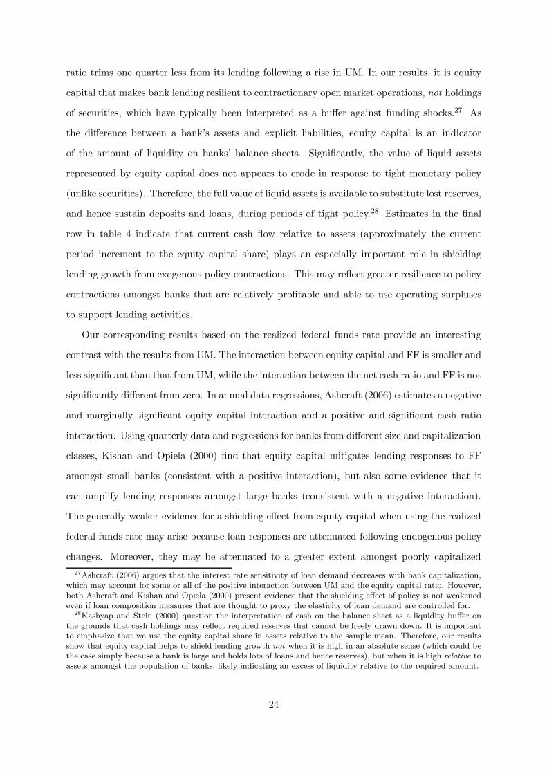
ratio trims one quarter less from its lending following a rise in UM. In our results, it is equity

capital that makes bank lending resilient to contractionary open market operations, not holdings

of securities, which have typically been interpreted as a buffer against funding shocks.27 As

the difference between a bank’s assets and explicit liabilities, equity capital is an indicator

of the amount of liquidity on banks’ balance sheets. Significantly, the value of liquid assets

represented by equity capital does not appears to erode in response to tight monetary policy

(unlike securities). Therefore, the full value of liquid assets is available to substitute lost reserves,

and hence sustain deposits and loans, during periods of tight policy.28 Estimates in the final

row in table 4 indicate that current cash flow relative to assets (approximately the current

period increment to the equity capital share) plays an especially important role in shielding

lending growth from exogenous policy contractions. This may reflect greater resilience to policy

contractions amongst banks that are relatively profitable and able to use operating surpluses

to support lending activities.

Our corresponding results based on the realized federal funds rate provide an interesting

contrast with the results from UM. The interaction between equity capital and FF is smaller and

less significant than that from UM, while the interaction between the net cash ratio and FF is not

significantly different from zero. In annual data regressions, Ashcraft (2006) estimates a negative

and marginally significant equity capital interaction and a positive and significant cash ratio

interaction. Using quarterly data and regressions for banks from different size and capitalization

classes, Kishan and Opiela (2000) find that equity capital mitigates lending responses to FF

amongst small banks (consistent with a positive interaction), but also some evidence that it

can amplify lending responses amongst large banks (consistent with a negative interaction).

The generally weaker evidence for a shielding effect from equity capital when using the realized

federal funds rate may arise because loan responses are attenuated following endogenous policy

changes. Moreover, they may be attenuated to a greater extent amongst poorly capitalized

27Ashcraft (2006) argues that the interest rate sensitivity of loan demand decreases with bank capitalization,which may account for some or all of the positive interaction between UM and the equity capital ratio. However,both Ashcraft and Kishan and Opiela (2000) present evidence that the shielding effect of policy is not weakenedeven if loan composition measures that are thought to proxy the elasticity of loan demand are controlled for.

28Kashyap and Stein (2000) question the interpretation of cash on the balance sheet as a liquidity buffer onthe grounds that cash holdings may reflect required reserves that cannot be freely drawn down. It is importantto emphasize that we use the equity capital share in assets relative to the sample mean. Therefore, our resultsshow that equity capital helps to shield lending growth not when it is high in an absolute sense (which could bethe case simply because a bank is large and holds lots of loans and hence reserves), but when it is high relative toassets amongst the population of banks, likely indicating an excess of liquidity relative to the required amount.

24

banks, since they likely expand loan supply more in response to the factors associated with

endogenous policy tightening (see the discussion in section 2.1).

We draw attention to two implications of our finding that well-capitalized banks are able to

shield their lending from exogenous monetary policy. First, banks that are unable to smooth

their lending using funds from associate networks (e.g., holding companies) may be able to

mitigate any lending contractions through the accumulation of equity capital buffers. At the

end of our sample, the average equity capital ratio for stand-alone banks is 4 percentage points

higher than for holding company banks, which is consistent with this idea (other interpretations

of this observation are possible – e.g., the probability of joining a holding company may be linked

to the equity capital ratio). Second, reductions in banking sector equity capital from loan write-

offs during the recent housing market collapse and credit crunch may leave banks less able to

shield their lending from contractionary monetary policy. This in turn may embed a more

powerful monetary transmission mechanism until banks restore their capitalization ratios to

levels seen prior to the current period of financial market turmoil.

4.1 Stability of the baseline results

An important issue in any study of monetary policy transmission to the banking sector is

the temporal stability of the results – see Bernanke and Blinder (1992), Kashyap and Stein

(2000) and Ashcraft (2006). In our sample, an important structural change may arise from

the introduction of the source of strength doctrine (Ashcraft, 2006).29 The Federal Reserve

Board issued a formal statement in April 1987 indicating that failure by a parent bank to inject

liquidity into a financially distressed subsidiary when funds are available would be considered

an unsafe banking practice.30

In section 3.2, we argued that from 1987 onwards membership in a bank holding company

should affect lending responses to monetary policy. Our baseline results are consistent with this

29Another source of structural change is the abolition of regulation Q, which restricted banks’ ability tovary interest rates in order to attract deposits (a source of funding). The abolition of this restriction waslargely implemented via the Monetary Control Act of 1980, and is therefore likely to induce heterogeneity in ourresults across a much shorter period than the source of strength doctrine. Due to the limitations in estimatingheterogeneity in our results across a period of just three years or so, we do not address the effects of regulationQ. If observations from this period exerted undue influence on the results, the outlier detection procedure weemploy ought to diagnose them.

30As noted in footnote 12, Ashcraft (2008) shows that the Financial Institutions Reform, Recovery, and En-forcement Act of 1989 unexpectedly strengthened the source of strength doctrine. Given that this change occurredjust two years after 1987, we do not allow for a further structural change in 1989.

25

idea. In this sub-section, we take our analysis of the effects of the source of strength of doctrine

one stage further. We interact each of the cross terms in∑4

j=0 X ′i,t−1Mq,t−jδq,j,∀q ∈ {1, 2, 3}

with a binary variable that is set to unity post-1986 for banks that belong to a holding company

(excluding the cross term that already features the holding company indicator). These extra

terms are added to our baseline regression in 3. In table 5, we report interaction coefficients for

policy measures and characteristics (similar to those in table 4), in addition to the changes to

the interaction coefficients associated with the start of the source of strength doctrine.

The key feature of the results is that the post-1986 changes to the interaction coefficients

(amongst holding company banks) are of approximately equal magnitude but opposite sign to

the main interaction effects (the one exception is the interaction of FF with bank assets). As

such, the total effect of balance sheet related characteristics on lending responses to monetary

policy, both exogenous and endogenous, is close to zero during the second half of the sample

for affiliated banks (and recall that affiliated banks represent over two thirds of all banks in

this period). During the late 1980s and the 1990s, the principal source of heterogeneity in

lending responses to monetary policy is affiliation with a holding company, not balance sheet

composition. The roles of security holdings in amplifying and equity capital in mitigating

the effects of exogenous policy on lending growth, are quantitatively smaller from the late

1980s onwards because they are observed only amongst banks that cannot access the financing

networks provided by holding companies. In contrast, when affiliated banks face write-downs in

securities prices or loan values following policy tightenings, they are able to tap loanable funds

within the network, thus shielding their lending growth.

4.2 Loan composition effects

In this sub-section, we consider information on the composition of bank loan books. The Call

Reports provide information on bank loans across five categories: residential loans, commercial

and industrial loans, individual (consumer) loans, agricultural loans and municipal loans – see

table 2 for some summary statistics relevant to our sample. This information is relevant to

lending responses for a number of reasons. First, loans that are at least partially collateralized

are more easily sold via the securitization process. In such instances, banks effectively serve as

warehouses for loans and may liquidate them in response to funding shocks (Strahan, 2008).31

31This has not been the case for sub-prime loans during the financial crisis that started in 2007.

26

Collateral is a more common feature of loans to customers in the residential and consumer

sectors. Banks concentrating in those areas may be more able to shield their lending growth

from monetary policy via securitization.32 Second, it is possible that the interest rate sensitivity

of loan demand varies across sectors of the market. For instance, the shorter maturity of

commercial and industrial loans may render them more responsive to monetary policy (Kishan

and Opiela, 2000). Equally, the pro-cyclicality of loan demand and loan supply, which we

discussed in section 2, may vary across sectors. For instance, consumer loan demand may

respond more strongly to income expectations. If such heterogeneity is a feature of the banking

system, it can be captured using information on loan composition.

We take the total loan shares for residential loans, consumer loans and commercial and

industrial loans, and introduce them as additional bank characteristics in our baseline regression,

equation 3. We consider just three elements of the loan decomposition from the Call Reports,

since municipal lending is typically a small share of total lending. The four remaining loan

categories account for almost 100% of bank lending and as such are nearly collinear. In order

to handle this, we omit the agricultural loan share. In table 6, we report output analogous to

that in table 4. The responsiveness of bank lending to a 100 b.p. tightening is reported for the

representative bank. We also report the increments to the lending response associated with a

loan share measure that is one standard deviation above the mean share for loans of that type.

We do not report results for the bank characteristics discussed previously, but they confirm

those presented in tables 3 and 4 (details available upon request).

Using changes in the realized federal funds rate, a bank whose participation in the residential

loan market is one standard deviation above the mean contracts their lending by roughly twice

as much as a bank that does an average amount of business in that market. A similar result

holds for banks whose business is concentrated in the consumer loans market. In contrast,

commercial lending is only slightly more responsive to federal funds rate rises than the average

loan, and by implication agricultural loans must be less responsive to policy than loans in

general. These results are consistent with those reported by Kishan and Opiela, who show that

residential and consumer lending at small and poorly capitalized banks contracts more rapidly

than commercial lending.

32Loutskina (2005) develops a more precise measure of the securitizability of bank loan books that incorporatesinformation on the extent of securitization of different loan categories at the aggregate level, as well as thecomposition of bank loan portfolios.

27

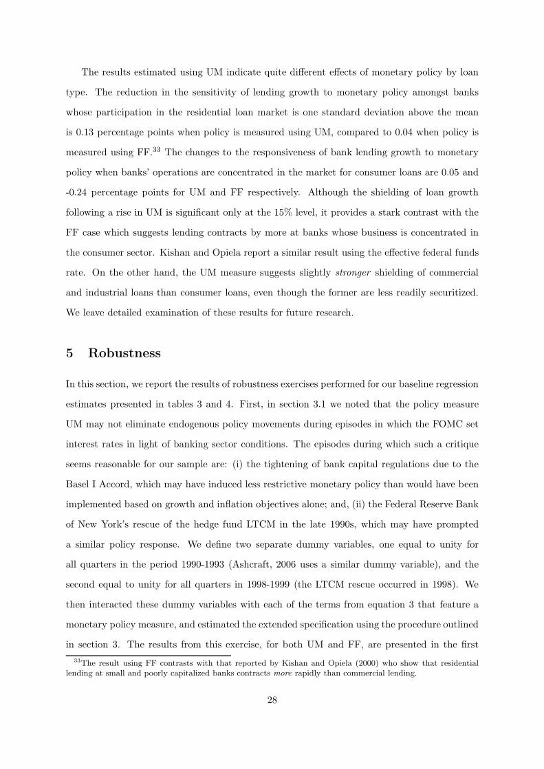
The results estimated using UM indicate quite different effects of monetary policy by loan

type. The reduction in the sensitivity of lending growth to monetary policy amongst banks

whose participation in the residential loan market is one standard deviation above the mean

is 0.13 percentage points when policy is measured using UM, compared to 0.04 when policy is

measured using FF.33 The changes to the responsiveness of bank lending growth to monetary

policy when banks’ operations are concentrated in the market for consumer loans are 0.05 and

-0.24 percentage points for UM and FF respectively. Although the shielding of loan growth

following a rise in UM is significant only at the 15% level, it provides a stark contrast with the

FF case which suggests lending contracts by more at banks whose business is concentrated in

the consumer sector. Kishan and Opiela report a similar result using the effective federal funds

rate. On the other hand, the UM measure suggests slightly stronger shielding of commercial

and industrial loans than consumer loans, even though the former are less readily securitized.

We leave detailed examination of these results for future research.

5 Robustness

In this section, we report the results of robustness exercises performed for our baseline regression

estimates presented in tables 3 and 4. First, in section 3.1 we noted that the policy measure

UM may not eliminate endogenous policy movements during episodes in which the FOMC set

interest rates in light of banking sector conditions. The episodes during which such a critique

seems reasonable for our sample are: (i) the tightening of bank capital regulations due to the

Basel I Accord, which may have induced less restrictive monetary policy than would have been

implemented based on growth and inflation objectives alone; and, (ii) the Federal Reserve Bank

of New York’s rescue of the hedge fund LTCM in the late 1990s, which may have prompted

a similar policy response. We define two separate dummy variables, one equal to unity for

all quarters in the period 1990-1993 (Ashcraft, 2006 uses a similar dummy variable), and the

second equal to unity for all quarters in 1998-1999 (the LTCM rescue occurred in 1998). We

then interacted these dummy variables with each of the terms from equation 3 that feature a

monetary policy measure, and estimated the extended specification using the procedure outlined

in section 3. The results from this exercise, for both UM and FF, are presented in the first

33The result using FF contrasts with that reported by Kishan and Opiela (2000) who show that residentiallending at small and poorly capitalized banks contracts more rapidly than commercial lending.

28

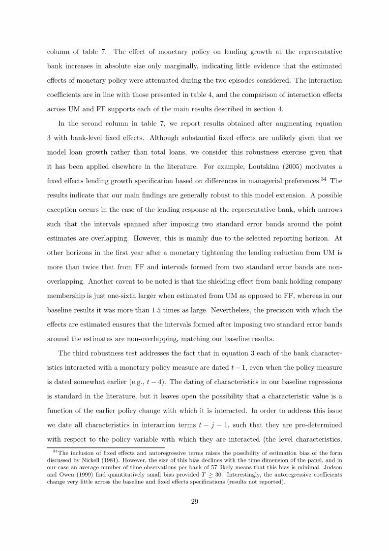
column of table 7. The effect of monetary policy on lending growth at the representative

bank increases in absolute size only marginally, indicating little evidence that the estimated

effects of monetary policy were attenuated during the two episodes considered. The interaction

coefficients are in line with those presented in table 4, and the comparison of interaction effects

across UM and FF supports each of the main results described in section 4.

In the second column in table 7, we report results obtained after augmenting equation

3 with bank-level fixed effects. Although substantial fixed effects are unlikely given that we

model loan growth rather than total loans, we consider this robustness exercise given that

it has been applied elsewhere in the literature. For example, Loutskina (2005) motivates a

fixed effects lending growth specification based on differences in managerial preferences.34 The

results indicate that our main findings are generally robust to this model extension. A possible

exception occurs in the case of the lending response at the representative bank, which narrows

such that the intervals spanned after imposing two standard error bands around the point

estimates are overlapping. However, this is mainly due to the selected reporting horizon. At

other horizons in the first year after a monetary tightening the lending reduction from UM is

more than twice that from FF and intervals formed from two standard error bands are non-

overlapping. Another caveat to be noted is that the shielding effect from bank holding company

membership is just one-sixth larger when estimated from UM as opposed to FF, whereas in our

baseline results it was more than 1.5 times as large. Nevertheless, the precision with which the

effects are estimated ensures that the intervals formed after imposing two standard error bands

around the estimates are non-overlapping, matching our baseline results.

The third robustness test addresses the fact that in equation 3 each of the bank character-

istics interacted with a monetary policy measure are dated t− 1, even when the policy measure

is dated somewhat earlier (e.g., t − 4). The dating of characteristics in our baseline regressions

is standard in the literature, but it leaves open the possibility that a characteristic value is a

function of the earlier policy change with which it is interacted. In order to address this issue

we date all characteristics in interaction terms t − j − 1, such that they are pre-determined

with respect to the policy variable with which they are interacted (the level characteristics,

34The inclusion of fixed effects and autoregressive terms raises the possibility of estimation bias of the formdiscussed by Nickell (1981). However, the size of this bias declines with the time dimension of the panel, and inour case an average number of time observations per bank of 57 likely means that this bias is minimal. Judsonand Owen (1999) find quantitatively small bias provided T ≥ 30. Interestingly, the autoregressive coefficientschange very little across the baseline and fixed effects specifications (results not reported).

29

which enter the regression just once, continue to be dated t− 1). The results from this exercise,

performed for both UM and FF, are reported in the third column in table 7.

Our main findings are robust, except in two cases. First, the amplification of the contrac-

tionary effects of UM associated with large security holdings is absent in the third set of results,

signaling the need for some caution in relation to this finding. Interestingly, the negative in-

teraction between UM and the securities ratio is observed if we cumulate the interaction terms

out to horizon 3 rather than horizon 4, and is present out to horizon 4 if we use the larger

sample that does not exclude outliers. Second, the interactions between the policy measures

and the net cash ratio change sign in column 3 relative to the baseline case. The effect of bank

profitability/cash flow on lending responses to monetary policy is more dependent on the dating

of the characteristic than are the effects of other characteristics. This is unsurprising since the

net cash ratio, closely linked to profits, is less persistent than other components of assets. It

therefore changes more through time (the relatively low persistence of this series is reflected in

its large coefficient of variation, calculable from table 2). One interpretation of our previous

result for the net cash ratio is that policy shocks exert a large and persistent effect on the lend-

ing of a certain group of banks, which then reduces their profitability and net cash ratio. The

relatively large lending reversal for this set of banks then correlates with a low equity capital

ratio, yielding the positively signed interaction from this characteristic in table 4. In table 7,

this positively signed interaction is absent because the characteristics are pre-determined with

respect to monetary policy and cannot respond to policy changes. Given this possible interpre-

tation of the net cash ratio interaction, we do not emphasize our results from this particular

characteristic, focusing instead on those related to total assets, holding company status, and

the balance sheet shares of securities and equity capital.

In the final column in table 7, we present a version of our baseline results that uses an

alternative definition of the total assets variable. This is the demeaned series for ln(

assetsi,t

assetst

)

where assetst is the cross-sectional mean of assets in period t (in the baseline case, we use the

demeaned series for ln (assetsi,t)). Scaling each observation by the cross-sectional mean of bank

assets at each point in time eliminates the drift in assets that occurs as a result of bank balance

sheets growing in nominal terms through time. In the baseline results, this effect was handled

via the inclusion of a time trend, an approach that is standard in the literature (e.g., Loutskina,

30

2005). Such a method will account for a linear trend in the assets of a representative bank, but

it does not deal with changes to the average growth rate for bank assets. We use the alternative

definition in all terms that feature assets (including the interaction terms), so that the new set

of results does not reflect any common, time-varying drift in the data for total assets.

Our core results remain intact using the new measure of assets, except that the interaction

between bank assets turns negative and marginally significant when UM is the policy measure,

and negative and significant when FF is the policy measure. It appears that the evidence

that large banks can shield their lending growth from monetary policy is partly a function

of the upward trend in asset values, which correlates with the trend towards weaker monetary

transmission through time. In the absence of this effect, notice how the impact of UM on lending

growth at the representative bank moderates from -0.94 to -0.74. Crucially however, our other

results are very robust in the final column in table 7. In particular, the lending contraction at

the representative bank is one-third larger when policy is measured using UM rather than FF.

Moreover, the shielding of lending growth amongst holding companies is 1.5 times larger using

the exogenous policy measure. Finally, it is the equity capital ratio, not the securities ratio,

that serves as a buffer to lending growth when monetary policy shocks are measured using UM.

6 Conclusions

The credit market turmoil of 2007 and 2008 has highlighted the critical role played by the bank-

ing system in the transmission of monetary policy to the real economy. Recently, policymakers

have focused on the way in which banking sector conditions have blunted the stabilizing effects

of the large interest rate reductions implemented by the FOMC during the first half of 2008

(Rosengren, 2008). During the last decade, considerable progress has been made in identifying

the features of the banking industry that matter for monetary transmission, especially following

the creation of the large database on the activities of FDIC-insured banks in the United States

in work by Kashyap and Stein (2000). The bulk of this research has used the realized federal

funds rate to measure monetary policy. The key point emphasized in our paper is that such a

policy measure is endogenous to expected future macroeconomic conditions, which are likely to

exert separate effects on both loan demand and loan supply. We have set out examples of such

effects and have argued that they may induce bias in both the estimated direct impact of mone-

31

tary policy on bank lending and in the estimated impact conditional upon bank characteristics.

In the empirics, we provided a comparison of the heterogeneity in bank lending responses to

an explicitly identified monetary policy measure and the realized interest rate which is more

commonly used in the literature.

The results indicated both economically and statistically significant attenuation of lending

responses to monetary contractions, accompanied by the shielding of lending associated with

bank holding company affiliation. We also found sign reversals in the effects conditional upon

some characteristics. Specifically, the share of securities in total assets was shown to amplify

policy transmission from exogenous interest rate changes, while restricting the transmission of

realized interest rate changes. One explanation for this result is that many types of securities

are subject to an adverse valuation effect following exogenous monetary policy contractions,

which limits the scope for lending at banks that hold them in large numbers. In contrast,

endogenous rises in the federal funds rate may be associated with lending increases (due to the

underlying macroeconomic conditions to which policy is endogenous) at banks which choose to

invest heavily in securities. The bank characteristic found to correlate with shielding of lending

growth after policy contractions was the equity capital ratio. This shielding effect was stronger

using the exogenous policy measure.

An important research implication from our work is that future studies of the banking

system and monetary transmission should consider exogenous policy measures, alongside other

measures such as the realized federal funds rate. In particular, the identification of exogenous

monetary policy should take into account the forward-looking drivers of monetary policy such

as growth and inflation forecasts, because these forward-looking variables are likely to impact

lending markets. Interesting avenues for future work include the examination of the impact of

exogenous monetary policy upon regional, industrial, and firm-specific lending. It would then

be possible to compare these impacts with those from the realized federal funds rate, and to

consider their consistency with the banking sector structure relevant to the associated regions,

industries, and firms. One possibility is that heterogeneity in the banking sector may account

for a larger proportion of the differential effects of monetary policy across these units when an

exogenous policy measure is employed (see section 4 discussion). Other interesting areas for

future work include the application of the methodology used here to study heterogeneity in

32

lending rates, as opposed to lending quantities. In addition, it would be useful to investigate

the effects of bank characteristics on responses to policy at a more disaggregated level, such as

the relationship to the particular mixture of securities held as bank assets.

References

Ashcraft, A. B. (2001): “New evidence on the lending channel,” Federal Reserve Bank of

New York Staff Report, (136).

(2006): “New evidence on the lending channel,” Journal of Money, Credit, and Bank-

ing, 38(3), 751–775.

(2008): “Are Bank Holding Companies a Source of Strength to Their Banking Sub-

sidiaries?,” Journal of Money, Credit, and Banking, 40(2-3), 273–294.

Bernanke, B., and M. Gertler (1989): “Agency Costs, Net Worth, and Business Fluctua-

tions,” American Economic Review, 79(1), 14–31.

Bernanke, B. S., and A. S. Blinder (1992): “The Federal Funds Rate and the Channels of

Monetary Transmission,” American Economic Review, 82(4), 901–921.

Bernanke, B. S., and J. Boivin (2003): “Monetary policy in a data-rich environment,”

Journal of Monetary Economics, 50(3), 525–546.

Bernanke, B. S., and M. L. Gertler (1995): “Inside the Black Box: The Credit Channel

of Monetary Policy Transmission,” Journal of Economic Perspectives, 9(4), 27–48.

Bernanke, B. S., and I. Mihov (1998): “Measuring Monetary Policy,” Quarterly Journal of

Economics, 113(3), 869–902.

Bluedorn, J. C., and C. Bowdler (2008): “The Open Economy Consequences of U.S.

Monetary Policy,” Manuscript, Universities of Southampton and Oxford.

Board of Governors of the Federal Reserve (2005): The Federal Reserve System

Purposes and Functions. Publications Fulfillment, Board of Governors of the Federal Reserve,

Washington, DC, USA, ninth edn.

33

Boivin, J., and M. Giannoni (2002): “Assessing changes in the monetary transmission mech-

anism: a VAR approach,” Federal Reserve Bank of New York Economic Policy Review, 8(1),

97–111.

Boschen, J. F., and L. O. Mills (1991): “The effects of countercyclical monetary policy

on money and interest rates: An evaluation of evidence from FOMC documents,” Federal

Reserve Bank of Philadelphia Working Paper, (91-20).

(1995): “The relation between narrative and money market indicators of monetary

policy,” Economic Inquiry, 33(1), 24–44.

Carlino, G., and R. DeFina (1998): “The Differential Regional Effects of Monetary Policy,”

Review of Economics and Statistics, 80(4), 572–587.

Cetorelli, N., and L. S. Goldberg (2008): “Banking Globalization, Monetary Transmis-

sion, and the Lending Channel,” NBER Working Paper, (14101).

Christiano, L. J., M. Eichenbaum, and C. L. Evans (1999): Handbook of Macroeco-

nomicsvol. 1 of Handbooks in Economics, chap. Monetary policy shocks: What have we

learned and to what end?, pp. 65–148. Elsevier B.V., Amsterdam, Netherlands.

Giordani, P. (2004): “An alternative explanation of the price puzzle,” Journal of Monetary

Economics, 51(6), 1271–1296.

Hancock, D., and J. A. Wilcox (1998): “The “credit crunch” and the availability of credit

to small business,” Journal of Banking and Finance, 22(6), 983–1014.

Houston, J., C. James, and D. Marcus (1997): “Capital market frictions and the role of

internal capital markets in banking,” Journal of Financial Economics, 46(2), 135–164.

Jonas, M. R., and S. K. King (2008): “Bank Efficiency and the Effectiveness of Monetary

Policy,” Contemporary Economic Policy, 26(4), 579–589.

Judson, R. A., and A. L. Owen (1999): “Estimating dynamic panel data models: a guide

for macroeconomists,” Economics Letters, 65(1), 9–15.

Kashyap, A. K., and J. C. Stein (2000): “What Do A Million Observations on Banks Say

About the Transmission of Monetary Policy?,” American Economic Review, 90(3), 407–428.

34

Kishan, R. P., and T. P. Opiela (2000): “Bank Size, Bank Capital, and the Bank Lending

Channel,” Journal of Money, Credit, and Banking, 32(1), 121–141.

Loutskina, E. (2005): “Does Securitization Affect Bank Lending? Evidence from Bank Re-

sponses to Funding Shocks,” Web.

Meulendyke, A.-M. (1998): U.S. Monetary Policy and Financial Markets. Federal Reserve

Bank of New York.

Morgan, D. P. (1998): “The Credit Effects of Monetary Policy: Evidence Using Loan Com-

mitments,” Journal of Money, Credit, and Banking, 30(1), 102–118.

Nickell, S. (1981): “Biases in Dynamic Models with Fixed Effects,” Econometrica, 49(6),

1417–1426.

Pagan, A. R. (1984): “Econometric Issues in the Analysis of Regressions with Generated

Regressors,” International Economic Review, 25, 221–248.

Peek, J., and E. S. Rosengren (1998): “Bank consolidation and small business lending: It’s

not just bank size that matters,” Journal of Banking and Finance, 22(6-8), 799–819.

Romer, C. D., and D. H. Romer (2000): “Federal Reserve Information and the Behavior of

Interest Rates,” American Economic Review, 90(3), 429–457.

(2004): “A New Measure of Monetary Shocks: Derivation and Implications,” American

Economic Review, 94(4), 1055–1084.

(2008): “The FOMC versus the Staff: Where Can Monetary Policymakers Add

Value?,” NBER Working Paper, (13751).

Rosengren, E. S. (2008): “Implications of a Credit Crunch,” Web, accessed 10 July 2009,

Speech delivered to the Business and Industry Association of New Hampshire and the Greater

Manchester Chamber of Commerce.

Strahan, P. (2008): “Liquidity Production in 21st Century Banking,” NBER Working Paper,

(13798).

35

Strongin, S. (1995): “The identification of monetary policy disturbances explaining the liq-

uidity puzzle,” Journal of Monetary Economics, 35(3), 463–497.

Welsch, R. E., and E. Kuh (1977): “Linear Regression Diagnostics,” NBER Working Paper,

(173).

Wooldridge, J. M. (2003): “Cluster-Sample Methods in Applied Econometrics,” American

Economic Review, 93(2), 133–138.

36

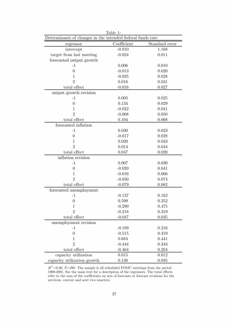
Table 1:Table 1

Determinants of changes in the intended federal funds rate

regressor Coefficient Standard error

intercept -0.910 1.168

target from last meeting -0.024 0.011

forecasted output growth

-1 0.006 0.010

0 -0.013 0.020

1 -0.025 0.028

2 0.016 0.031

total effect -0.016 0.027

output growth revision

-1 0.005 0.025

0 0.134 0.029

1 -0.022 0.041

2 -0.008 0.050

total effect 0.104 0.068

forecasted inflation

-1 0.030 0.023

0 -0.017 0.028

1 0.020 0.043

2 0.014 0.044

total effect 0.047 0.020

inflation revision

-1 0.007 0.030

0 -0.020 0.041

1 -0.016 0.066

2 -0.050 0.074

total effect -0.079 0.082

forecasted unemployment

-1 -0.137 0.162

0 0.599 0.352

1 -0.290 0.475

2 -0.218 0.319

total effect -0.047 0.035

unemployment revision

-1 -0.189 0.216

0 -0.515 0.319

1 0.684 0.441

2 -0.444 0.343

total effect -0.464 0.204

capacity utilization 0.015 0.012

capacity utilization growth 0.136 0.035

R2=0.36, N=298. The sample is all scheduled FOMC meetings from the period

1969-2001. See the main text for a description of the regressors. The total effects

refer to the sum of the coefficients on sets of forecasts or forecast revisions for the

previous, current and next two quarters.

37

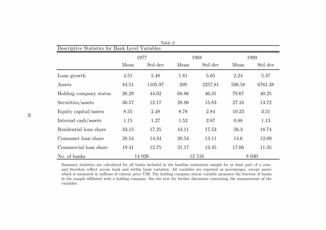
Table 2:Table 2Descriptive Statistics for Bank Level Variables

1977 1988 1999

Mean Std dev Mean Std dev Mean Std dev

Loan growth 4.51 5.48 1.81 5.65 2.24 5.47

Assets 84.51 1105.97 209 2257.81 506.58 6761.38

Holding company status 26.29 44.02 68.86 46.31 79.67 40.25

Securities/assets 30.57 12.17 28.86 15.83 27.16 13.72

Equity capital/assets 8.55 2.48 8.78 2.84 10.23 3.51

Internal cash/assets 1.15 1.27 1.52 2.87 0.88 1.13

Residential loan share 33.15 17.25 44.11 17.53 56.3 18.74

Consumer loan share 28.54 14.34 20.54 13.11 14.6 12.09

Commercial loan share 19.41 12.75 21.17 13.45 17.06 11.35

No. of banks 14 026 12 516 8 030

Summary statistics are calculated for all banks included in the baseline estimation sample for at least part of a year,and therefore reflect across bank and within bank variation. All variables are reported as percentages, except assetswhich is measured in millions of current price US$. The holding company status variable measures the fraction of banksin the sample affiliated with a holding company. See the text for further discussion concerning the measurement of thevariables.

38

Table 3:Table 3Lending Responses at the Representative Bank

Horizon UM FF

0 -0.04* -0.03**(0.02) (0.005)

1 -0.40** -0.18**(0.02) (0.009)

2 -0.75** -0.38**(0.04) (0.014)

3 -0.92** -0.60**(0.05) (0.02)

4 -0.94** -0.73**(0.05) (0.02)

Notes: Cumulative responses to a 100b.p. tightening atthe specified horizon are reported for a bank at thesample average of continuously measuredcharacteristics and not part of a holding company.Standard errors after clustering at the bank level arereported in parentheses. ** and * indicate significanceat the 1% and 5% levels respectively.

39

Table 4:Table 4

Bank Lending Responses to Monetary Policy

UM FF

representative bank

marginal effect -0.94** -0.73**

(0.05) (0.02)

assets

interaction 0.26** 0.08**

(0.03) (0.01)

marginal effect -0.68** -0.66**(0.06) (0.03)

holding company status

interaction 1.88** 1.21**

(0.08) (0.04)

marginal effect 0.95** 0.47**(0.07) (0.03)

securities ratio

interaction -0.22** 0.04*

(0.04) (0.02)

marginal effect -1.16** -0.69**(0.06) (0.03)

equity capital ratio

interaction 0.24** 0.04**

(0.04) (0.016)

marginal effect -0.70** -0.69**(0.06) (0.03)

net cash ratio

interaction 0.97** 0.08

(0.26) (0.14)

marginal effect 0.03 -0.65**(0.30) (0.13)

Observations 1053334 1052453

R 20.16 0.16

Notes: The reported lending responses are the sum ofcontemporaneous and four lagged responses to a 100 b.p. policytightening. Interaction effects are calculated for a bank onestandard deviation above the sample average for a characteristicand marginal effects sum the direct and interacted effects.Standard errors obtained after clustering at the bank level arereported in parentheses. ** and * indicate significance at the 1%and 5% levels respectively.

40

Table 5:Table 5

Holding Company Status and Lending Responses to Monetary Policy

UM FF

representative bank

marginal effect -0.81** -0.70**

(0.06) (0.02)

holding company status

interaction with policy 1.60** 1.09**

(0.10) (0.04)

assets

interaction with policy 0.48** 0.03(0.04) (0.02)

interaction with policy -0.65** 0.09**and holding company (0.07) (0.03)

securities ratio

interaction -0.57** 0.04*

(0.05) (0.02)

interaction with policy 0.76** -0.07and holding company (0.08) (0.03)

equity capital ratio

interaction 0.21** 0.07**

(0.04) (0.02)

interaction with policy -0.14 -0.09**and holding company (0.08) (0.03)

net cash ratio

interaction 1.40** 0.14

(0.27) (0.09)

interaction with policy -1.12** -0.19and holding company (0.40) (0.12)

Observations 1053673 1052665

R 20.16 0.16

Notes: The reported lending responses are the sum of contemporaneous and fourlagged responses to a 100 b.p. policy tightening. Interaction effects are calculatedfor a bank one standard deviation above the sample average for a characteristic.Standard errors obtained after clustering at the bank level are reported inparentheses. ** and * indicate significance at the 1% and 5% levels respectively.

41

Table 6:Table 6

Monetary Policy and the Structure of Bank Lending

UM FF

representative bank

marginal effect -0.80** -0.70**

(0.05) (0.02)

residential

interaction 0.13** 0.04*

(0.04) (0.02)

marginal effect -0.66** -0.66**(0.06) (0.03)

consumer

interaction 0.05 -0.24**

(0.03) (0.02)

marginal effect -0.74** -0.94**(0.05) (0.03)

commercial

interaction 0.08* -0.003

(0.04) (0.02)

marginal effect -0.71** -0.70**(0.06) (0.03)

Observations 1050736 1049694

R 20.17 0.17

Notes: The reported lending responses are the sum ofcontemporaneous and four laggeed responses to a 100 b.p. policytightening. Interaction effects are calculated for a bank onestandard deviation above the sample average for a given loanshare and marginal effects sum the direct and interacted effects.Standard errors obtained after clustering at the bank level arereported in parentheses. ** and * indicate significance at the 1%and 5% levels respectively.

42

Table 7:

Robustness Tests for the Baseline Model

ROBUSTNESS BASEL & LTCM FIXED PRE-DETERMINED SCALE TOTAL

TEST EPISODES EFFECTS CHARACTERISTICS ASSETS

UM FF UM FF UM FF UM FF

representative bank

marginal effect -0.96** -0.77** -0.86** -0.75** -0.88** -0.69** -0.74** -0.55**

(0.06) (0.02) (0.05) (0.02) (0.04) (0.02) (0.06) (0.02)

assets

interaction 0.29** -0.01 0.24** 0.04** 0.43** 0.09** -0.05* -0.09**

(0.03) (0.01) (0.03) (0.01) (0.03) (0.01) (0.03) (0.01)

holding company status

interaction 1.56** 0.96** 1.53** 1.24** 1.69** 1.08** 1.79** 1.19**

(0.10) (0.05) (0.08) (0.04) (0.08) (0.03) (0.08) (0.03)

securities ratio

interaction -0.36** 0.06** -0.15** 0.1** -0.01 0.06** -0.23** 0.04*

(0.04) (0.02) (0.04) (0.02) (0.03) (0.01) (0.04) (0.02)

equity capital ratio

interaction 0.09* 0.01 0.28** 0.04** 0.12** 0.01 0.08* 0.002

(0.04) (0.02) (0.04) (0.02) (0.03) (0.01) (0.04) (0.01)

net cash ratio

interaction 1.60** 0.08 0.98** 0.01 -0.74** -0.05* 1.31** 0.03

(0.22) (0.09) (0.25) (0.10) (0.14) (0.02) (0.29) (0.18)

Observations 1054328 1053721 1053334 1052453 1032780 1031899 1053403 1052489

R 20.16 0.16 0.13 0.13 0.16 0.16 0.16 0.16

Notes: The reported lending responses are the sum of contemporaneous and four laggeed responses to a 100 b.p. policy tightening. Interactioneffects are calculated for a bank one standard deviation above the sample average for a given characteristic. Marginal effects sum the direct andinteracted effects. Standard errors obtained after clustering at the bank level are reported in parentheses. ** and * indicate significance at the1% and 5% levels respectively.

43

Figure 1: Time Series Plots for UM and FF

-10

-50

510

1975q1 1980q1 1985q1 1990q1 1995q1 2000q1date

um ff

Notes: Variables are defined as in the main text. The correlation of UM and FF over the sample in the figure is 0.60. The sample variance of UM is 0.76 percentage points (76 basis points) and the sample variance of FF is 1.57 percentage points (157 basis points).

44