Agent Objectives for Evolving Coordinated Sensor Networks
93
Transcript of Agent Objectives for Evolving Coordinated Sensor Networks


Agent Objectives for Evolving Coordinated Sensor Networks
by
Christian RothElectrical Engineering/Information Technology
170498-EIM
A MASTERS THESIS
submitted to
University of Applied Sciences O�enburg, E+IProf. Dr.-Ing. Peter Hildenbrand
in association withDr. Kagan Tumer, Ph.D.Oregon State University
in partial ful�llment ofthe requirements for the
degree of
Master of Engineering
April 15 - October 1, 2010

c©Copyright by Christian RothOctober 1, 2010
All Rights Reserved

AN ABSTRACT OF THE MASTERS THESIS OF
Christian Roth for the degree of Master of Engineering in
Electrical Engineering/Information Technology presented on October 1, 2010.
Title: Agent Objectives for Evolving Coordinated Sensor Networks
This Master's Thesis discusses intelligent sensor networks considering
autonomous sensor placement strategies and system health management. Sensor
networks for an intelligent system design process have been researched recently.
These networks consist of a distributed collective of sensing units, each with the
abilities of individual sensing and computation. Such systems can be capable of
self-deployment and must be scalable, long-lived and robust. With distributed
sensor networks, intelligent sensor placement for system design and online system
health management are attractive areas of research. Distributed sensor networks
also cause optimization problems, such as decentralized control, system
robustness and maximization of coverage in a distributed system. This also
includes the discovery and analysis of points of interest within an environment.
The purpose of this study was to investigate a method to control sensor
placement in a world with several sources and multiple types of information
autonomously. This includes both controlling the movement of sensor units and
�ltering of the gathered information depending on individual properties to
increase system performance, de�ned as a good coverage. Additionally, online
system health management was examined in this study regarding the case of
agent failures and autonomous policy recon�guration if sensors are added to or

removed from the system. Two di�erent solution strategies were devised, one
where the environment was fully observable, and one with only partial
observability. Both strategies use evolutionary algorithms based on arti�cial
neural networks for developing control policies. For performance measurement
and policy evaluation, di�erent multiagent objective functions were investigated.
The results of the study show that in the case of a world with multiple types of
information, individual control strategies performed best because of their abilities
to control the movement of a sensor entity and to �lter the sensed information.
This also includes system robustness in case of sensor failures where other sensing
units must recover system performance. Additionally, autonomous policy
recon�guration after adding or removing of sensor agents was successful. This
highlights that intelligent sensor agents are able to adapt their individual control
policies considering new circumstances.

EINE KURZFASSUNG DER MASTERS THESIS VON
Christian Roth für den Abschluss Master of Engineering in
Elektrotechnik/Informationstechnik eingereicht am 1. Oktober 2010.
Titel: Agent Objectives for Evolving Coordinated Sensor Networks
Diese Master Thesis betrachtet intelligente Sensornetzwerke unter den Aspekten
der selbständigen Sensorplatzierung und einer aktiven Überwachung des
Systemzustands. Sensornetzwerke für einen intelligenten Systemdesignprozess
werden seit einigen Jahren genauer untersucht. Diese Netzwerke bestehen aus
einer verteilten Ansammlung von Sensoreinheiten, jede mit den Eigenschaften
Informationen individuell aufzunehmen und zu verarbeiten. Solch eine
Anordnung kann die Fähigkeit besitzen, sich selbst zu strukturieren. Des
Weiteren müssen diese Systeme skalierbar, langlebend und widerstandsfähig sein.
Daraus ergeben sich interessante Forschungsaufgaben bezüglich der intelligenten
Anordnung von Sensoren während des Designprozesses oder einer aktive
Überwachung des Systemzustands im laufenden Betrieb. Diese Sensornetzwerke
bringen jedoch auch Optimierungsprobleme mit sich. Dazu zählen dezentralisierte
Regelungen, Gewährleistung der Widerstandsfähigkeit und Maximierung der
Abdeckung von Informationsquellen. Zusätzlich müssen Informationsquellen und
anderen Sensoreinheiten lokalisiert und analysiert werden können. Das Ziel dieser
Arbeit war es, eine Methode zu entwickeln, welche die Anordnung von Sensoren
in einer Umgebung mit Informationsquellen und verschiedenen Informationstypen
selbstständig bewerkstelligt. Dies beinhaltet zum einen die Regelung der

Bewegung dieser Sensoreinheiten und zum anderen die Filterung der
aufgenommen Informationen, entsprechend der Sensoreigenschaften. Dadurch
wird sicher gestellt, dass die Qualität des Systems gesteigert wird, was soviel
bedeutet wie eine gute Abdeckung der Informationsquellen. Zusätzlich wurde in
dieser Arbeit die aktive Systemüberwachung bezüglich Widerstandsfähigkeit im
Falle von Sensorfehlern und die selbstständige Anpassung der Regelstrategie nach
dem Hinzufügen oder Entfernen von Sensoren untersucht. Zwei unterschiedliche
Lösungsansätze wurden in dieser Arbeit ausgearbeitet. Zum einen war die
Umgebung komplett beobachtbar und zum anderen ein Ansatz in dem die
Sensoreinheiten nur über beschränkte Informationen verfügen. Beide
Lösungsansätze verwenden einen evolutionären Algorithmus, basierend auf
künstlichen Neuronalen Netzen. Des Weiteren wurden Multiagent Zielfunktionen
untersucht um die Qualität des Systems zu messen und die Regelstrategien zu
bewerten. Die Ergebnisse dieser Arbeit zeigen, dass im Falle einer Umgebung mit
mehreren Informationstypen, individuelle Regelungsstrategien die besten
Ergebnisse erzielen, weil diese Strategien sowohl in der Lage sind die Bewegung
der Sensoragenten zu kontrollieren, als auch die aufgenommenen Informationen
entsprechend der eigenen Eigenschaften zu �ltern. Zusätzlich zu diesen
Ergebnissen zeigt diese Arbeit eine selbstständige Anpassung der Regelstrategie
wenn Sensoragenten hinzugefügt oder entfernt wurden. Dies macht deutlich, dass
intelligente Sensoragenten in der Lage sind ihre individuellen Regelstrategien
entsprechend neuen Umständen anzupassen.

ACKNOWLEDGEMENTS
It is a pleasure to thank those who made this thesis possible, especially Dr.
Kagan Tumer who gave me the opportunity to write my Master's Thesis at
Oregon State University and helped me a lot with his advice. I also owe my
deepest gratitude to Dr. Matthew Knudson. Without his guidance and support,
this thesis would not be possible. I would like to extend my thanks to Dr.-Ing.
Peter Hildenbrand for all the time he has given toward my education.
Additionally, I would like to thank all my friends and colleagues for their
encouragement and support.

EIDESSTATTLICHE ERKLÄRUNG
Hiermit versichere ich eidesstattlich, dass die vorliegende Thesis von mir
selbstständig und ohne unerlaubte fremde Hilfe angefertigt worden ist,
insbesondere, dass ich alle Stellen, die wörtlich oder annähernd wörtlich oder dem
Gedanken nach aus Verö�entlichungen, unverö�entlichten Unterlagen und
Gesprächen entnommen worden sind, als solche an den entsprechenden Stellen
innerhalb der Arbeit durch Zitate kenntlich gemacht habe, wobei in den Zitaten
jeweils der Umfang der entnommenen Originalzitate kenntlich gemacht wurde.
Ich bin mir bewusst, dass eine falsche Versicherung rechtliche Folgen haben wird.
Datum, Unterschrift
Diese Thesis ist urheberrechtlich geschützt, unbeschadet dessen wird folgenden
Rechtsübertragungen zugestimmt:
• der Übertragung des Rechts zur Vervielfältigung der Thesis für Lehrzwecke
an der Hochschule O�enburg (�16 UrhG),
• der Übertragung des Vortrags-, Au�ührungs- und Vorführungsrechts für
Lehrzwecke durch Professoren der Hochschule O�enburg (�19 UrhG),
• der Übertragung des Rechts auf Wiedergabe durch Bild- oder Tonträger an
die Hochschule O�enburg (�21 UrhG).

DEDICATION
I dedicate this thesis to my parents,
Hildegard and Klaus Peter Roth,
for their love and support in my life.

TABLE OF CONTENTS
Page
1 Introduction 1
1.1 Motivation . . . . . . . . . . . . . . . . . . . . . . . . . . . . . . . . 1
1.2 Thesis Overview . . . . . . . . . . . . . . . . . . . . . . . . . . . . . 3
2 Background 5
2.1 Single Learning Agent . . . . . . . . . . . . . . . . . . . . . . . . . 5
2.2 Multiagent Systems . . . . . . . . . . . . . . . . . . . . . . . . . . . 7
2.3 Objective Functions in a Multiagent System . . . . . . . . . . . . . 8
2.4 Neuro-Evolution . . . . . . . . . . . . . . . . . . . . . . . . . . . . . 102.4.1 Arti�cial Neural Networks . . . . . . . . . . . . . . . . . . . 102.4.2 Evolutionary Algorithms . . . . . . . . . . . . . . . . . . . . 14
3 Problem Domain 17
3.1 Problem Description . . . . . . . . . . . . . . . . . . . . . . . . . . 17
3.2 Modeling the World . . . . . . . . . . . . . . . . . . . . . . . . . . . 19
3.3 Agent De�nition . . . . . . . . . . . . . . . . . . . . . . . . . . . . 20
3.4 Source Coverage . . . . . . . . . . . . . . . . . . . . . . . . . . . . . 21
3.5 Global Objective Function . . . . . . . . . . . . . . . . . . . . . . . 24
4 Fully Observable World 25
4.1 Agent Sensing . . . . . . . . . . . . . . . . . . . . . . . . . . . . . . 25
4.2 Agent Mapping . . . . . . . . . . . . . . . . . . . . . . . . . . . . . 28
4.3 Agent Action . . . . . . . . . . . . . . . . . . . . . . . . . . . . . . 29
4.4 Agent Learning and Objective . . . . . . . . . . . . . . . . . . . . . 29
5 Partially Observable World 30
5.1 Agent Sensing . . . . . . . . . . . . . . . . . . . . . . . . . . . . . . 30
5.2 Agent Mapping . . . . . . . . . . . . . . . . . . . . . . . . . . . . . 335.2.1 Agent Mapping using Deterministic Method . . . . . . . . . 335.2.2 Agent Mapping using Arti�cial Neural Networks . . . . . . . 34
5.3 Agent Action . . . . . . . . . . . . . . . . . . . . . . . . . . . . . . 35

TABLE OF CONTENTS (Continued)
Page
5.4 Agent Learning and Objectives . . . . . . . . . . . . . . . . . . . . 36
6 Experiments 38
6.1 Experiment De�nition . . . . . . . . . . . . . . . . . . . . . . . . . 39
6.2 World with Single Type of Information . . . . . . . . . . . . . . . . 41
6.3 World with Multiple Types of Information . . . . . . . . . . . . . . 51
6.4 System Robustness . . . . . . . . . . . . . . . . . . . . . . . . . . . 58
6.5 Policy Recon�guration . . . . . . . . . . . . . . . . . . . . . . . . . 61
6.6 Discussion . . . . . . . . . . . . . . . . . . . . . . . . . . . . . . . . 64
7 Conclusion 65
7.1 Contributions . . . . . . . . . . . . . . . . . . . . . . . . . . . . . . 65
7.2 Future Work . . . . . . . . . . . . . . . . . . . . . . . . . . . . . . . 66
Bibliography 69
Appendices 72
A List of Symbols . . . . . . . . . . . . . . . . . . . . . . . . . . . . . . 73
B Experiment Parameters . . . . . . . . . . . . . . . . . . . . . . . . . . 74

LIST OF FIGURES
Figure Page
2.1 A single agent framework where an agent observes the state of theenvironment and performs an action depending on its policy. Thereward signal applies to rank the agent's policy. . . . . . . . . . . . 6
2.2 Topology of a two-layer, feed forward network with i input units, jhidden units, o output units and weighted links with weight factorswi,j and wj,o. . . . . . . . . . . . . . . . . . . . . . . . . . . . . . . 11
2.3 Output computation of a processing unit with weighted inputs andbias by an activation function. . . . . . . . . . . . . . . . . . . . . . 12
2.4 Activation functions: (left) threshold function (Equation 2.4), (cen-ter) partial linear function (Equation 2.5), (right) sigmoid function(Equation 2.6) . . . . . . . . . . . . . . . . . . . . . . . . . . . . . . 13
2.5 Agent interacting with the environment by observing the state andperforming an action. An evolutionary algorithm applies to selecta network from the network population. The �tness of the cur-rent network is ranked by an objective function with regard to thepopulation. . . . . . . . . . . . . . . . . . . . . . . . . . . . . . . . 14
3.1 Two dimensional plane area with randomly distributed sources andagents constrained by a border on all edges. . . . . . . . . . . . . . 18
3.2 Drop o� functions: (left) source drop o� function (+1.0|100.0|5.0|0.5)(right) agent drop o� function (−1.0|20.0|5.0|0.5) . . . . . . . . . . 19
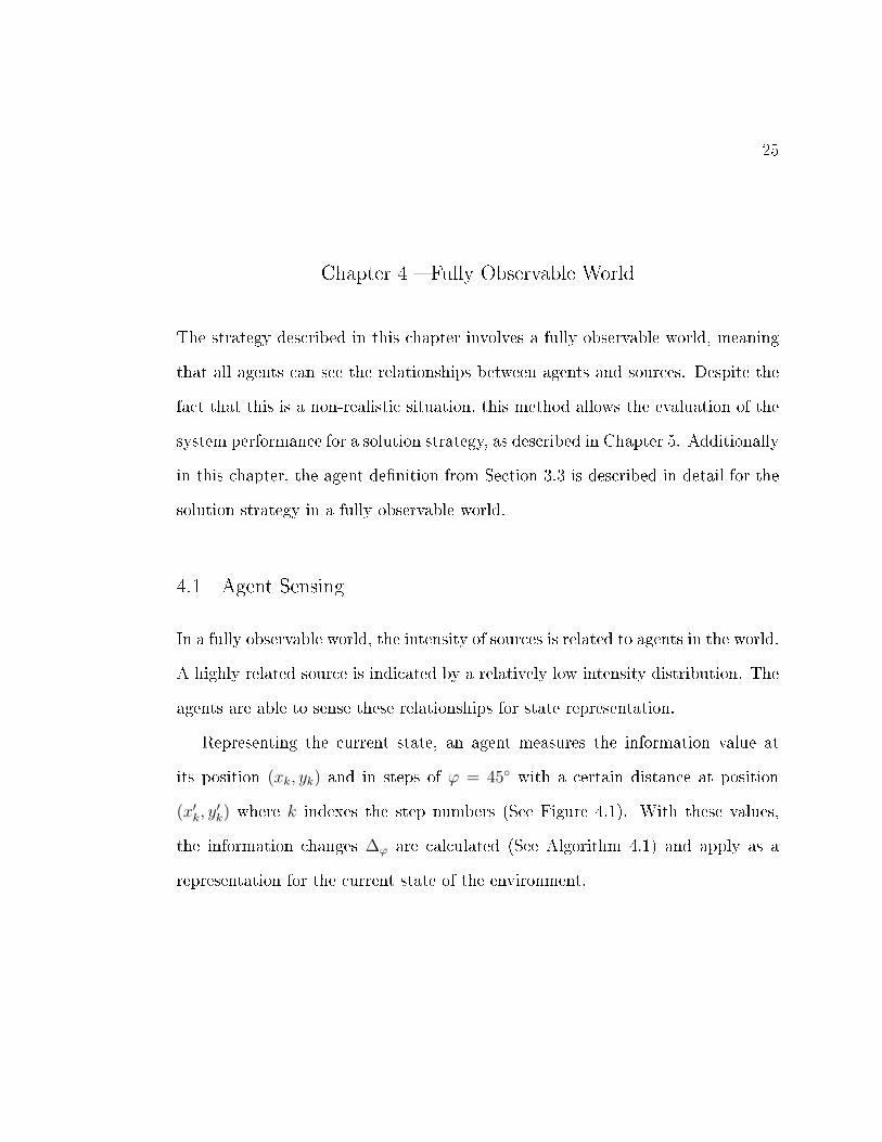
3.3 Example for the relationship of an agent to a source. This relation-ship is indicated by a lower amplitude of the source drop o� functionin the bottom picture. . . . . . . . . . . . . . . . . . . . . . . . . . 23
4.1 Sensing in a fully observable word. The agent senses the informationvalue at its current position (xk, yk) and around its position in stepsof ϕ = 45◦ (x′k, y
′k) to calculate the information change values ∆ϕ. . 26
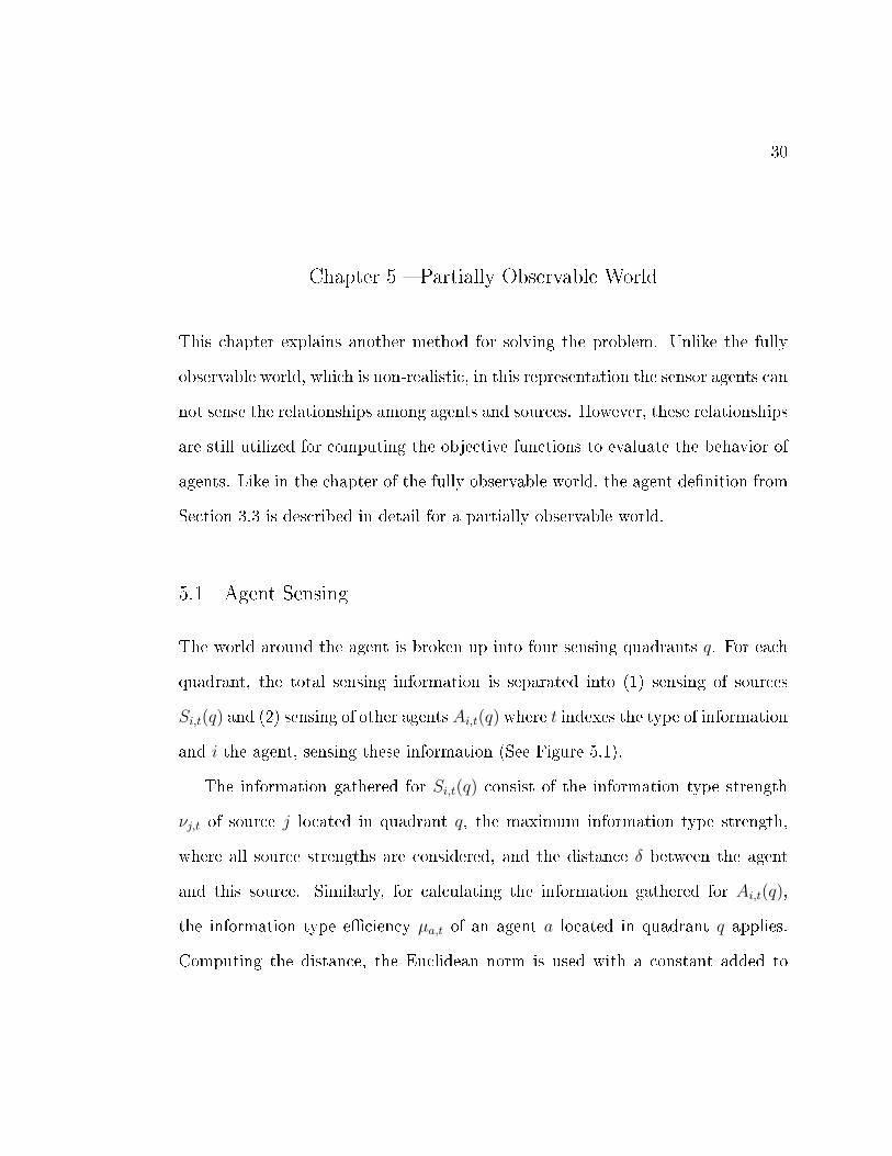
5.1 Sensing structure of agent i in a partially observable world. Theinformation is separated into four quadrants. For each quadrantthere is a sensor for agent-information and source-information. . . . 31
5.2 Linear cut o� functions: (left) for Si,t(q) (right) for Ai,t(q). Theseguarantee that the values are within a range between 0.0 and 1.0 . . 32

LIST OF FIGURES (Continued)
Figure Page
5.3 Linear, deterministic quality assignment for single type of informa-tion. The maximum quality value is assigned if the amount of sourceinformation is maximum and the amount of agent information isminimum. . . . . . . . . . . . . . . . . . . . . . . . . . . . . . . . . 34
6.1 Neural Network surfaces for a shared policy and three individualpolicies trained with the di�erence objective function (5 sources and15 agents): (left-top) shared policy, (right-top) individual policywith low e�ciency, (right-bottom) individual policy with mediume�ciency, (right-bottom) individual policy with high e�ciency . . . 42
6.2 Agents movement within a two dimensional, single information typeworld with 5 sources (S0...S4) and 10 agents (A0...A9) and partialobservability. More agents are located on sources S2 and S3 becauseof their high type strength (See Table B.1). . . . . . . . . . . . . . . 44
6.3 Results in a world with a single type of information for a con�gura-tion of 10 agents and 5 sources. The graphs show the developmentof shared policies compared to a hand coded policy in a partiallyobservable world. After 1000 episodes the ε-greedy network selec-tion is set to 0% meaning that the best ranked network is used allthe time. . . . . . . . . . . . . . . . . . . . . . . . . . . . . . . . . . 45
6.4 Results in a world with a single type of information for a con�gura-tion of 10 agents and 5 sources. The graphs show the developmentof individual policies in a partially observable world. After 1000episodes the ε-greedy network selection is set to 0% meaning thatthe best ranked network is used all the time. . . . . . . . . . . . . . 46
6.5 Results in a world with a single type of information for a con�gura-tion of 20 agents and 5 sources. The graphs show the developmentof shared policies compared to a hand coded policy in a partiallyobservable world. After 1000 episodes the ε-greedy network selec-tion is set to 0% meaning that the best ranked network is used allthe time. . . . . . . . . . . . . . . . . . . . . . . . . . . . . . . . . . 47

LIST OF FIGURES (Continued)
Figure Page
6.6 Results in a world with a single type of information for a con�gura-tion of 20 agents and 5 sources. The graphs show the developmentof individual policies in a partially observable world. After 1000episodes the ε-greedy network selection is set to 0% meaning thatthe best ranked network is used all the time. . . . . . . . . . . . . . 48
6.7 Maximum achieved G(z) for the applied algorithms and �tness func-tions in a world with a single type of information. The number ofagents starts with 5 agents and increases in steps of 5 agents to 30agents . . . . . . . . . . . . . . . . . . . . . . . . . . . . . . . . . . 49
6.8 Agents movement within a two dimensional, multiple informationtypes world with 5 sources (S0...S4) and 10 agents (A0...A9) andpartial observability. The parameters are given in Table B.2. . . . . 51
6.9 Results in a world with multiple types of information for a con�gu-ration of 10 agents and 5 sources. The graphs show the developmentof shared policies compared to a hand coded policy in a partiallyobservable world. After 1000 episodes the ε-greedy network selec-tion is set to 0% meaning that the best ranked network is used allthe time. . . . . . . . . . . . . . . . . . . . . . . . . . . . . . . . . . 53
6.10 Results in a world with multiple types of information for a con�gura-tion of 10 agents and 5 sources. The graphs show the developmentof individual policies in a partially observable world. After 1000episodes the ε-greedy network selection is set to 0% meaning thatthe best ranked network is used all the time. . . . . . . . . . . . . . 54
6.11 Results in a world with multiple types of information for a con�gu-ration of 20 agents and 5 sources. The graphs show the developmentof shared policies compared to a hand coded policy in a partiallyobservable world. After 1000 episodes the ε-greedy network selec-tion is set to 0% meaning that the best ranked network is used allthe time. . . . . . . . . . . . . . . . . . . . . . . . . . . . . . . . . . 55
6.12 Results in a world with multiple types of information for a con�gura-tion of 20 agents and 5 sources. The graphs show the developmentof individual policies in a partially observable world. After 1000episodes the ε-greedy network selection is set to 0% meaning thatthe best ranked network is used all the time. . . . . . . . . . . . . . 56

LIST OF FIGURES (Continued)
Figure Page
6.13 Maximum achieved G(z) for the applied algorithms and �tness func-tions in a world with multiple types of information. The number ofagents starts with 5 agents and increases in steps of 5 agents to 30agents . . . . . . . . . . . . . . . . . . . . . . . . . . . . . . . . . . 57
6.14 Reorganization of agents after 5 agents failed (Step 750) was possi-ble. The system performance could be partially recovered. Individ-ual policies were trained with the di�erence objective in a partiallyobservable world. . . . . . . . . . . . . . . . . . . . . . . . . . . . . 59
6.15 Reorganization of agents after 5 agents failed (Step 750) was notpossible. The system performance could not be recovered. Individ-ual policies were trained with the di�erence objective in a partiallyobservable world. . . . . . . . . . . . . . . . . . . . . . . . . . . . . 60
6.16 Recon�guration after removing agents at episode 500. For compar-ison, the learning graphs for 10 and 15 agents are also displayed. . . 62
6.17 Recon�guration after adding agents at episode 500. For comparison,the learning graphs for 15 and 20 agents are also displayed. . . . . . 63

LIST OF ALGORITHMS
Algorithm Page
2.1 ε-greedy Evolutionary Algorithm to determine Neural Network weights 15
3.1 Calculation of the Information type Coverage for each Source . . . . 22
3.2 Relationship among Agents and Sources for all types of Information . 22
4.1 Fully Observable World: Get Information changes for each Agent . . 27
4.2 Fully Observable World: Information Value for Agent i at a certain
Position weighted with its own E�ciencies. I(x, y, µi,t) . . . . . . . . 27
4.3 Fully Observable World: Dynamic Input Compression for Neural Net-
work . . . . . . . . . . . . . . . . . . . . . . . . . . . . . . . . . . . . 28

Chapter 1 � Introduction
This chapter introduces the motivation of this thesis and provides related work
from the �eld of distributed sensor networks. Additionally, an overview explains
the structure of this thesis.
1.1 Motivation
In large energy systems (e.g. power plants) an increasing number of sensors is
essential to achieve good control behavior and system safety. Sensors in these
energy systems might be temperature or pressure sensors, but it is also possible
that a highly developed sensing entity is able to sense multiple types of information
from the same location.
Distributed sensor groups which communicate with a centralized controller to
increase the system performance have been largely researched. However, this ap-
proach is often ine�cient because a lot of communication among sensors and the
controller is necessary, which a�ects the communication bandwidth. Instead of
using a centralized controller in a large energy system it can be more e�cient to
control the behavior of sensors with individual, non-centralized policies for intelli-
gent sensor units.

2
Related work in this domain addresses the description of sensor networks [1].
This includes a de�nition of the term 'coverage' in such networks [2] [3] [4]. In [5],
methods for an optimal sensor coverage with a minimum number of sensors is
provided. A better strategy may be to have an over-coverage (redundancy), to
recover system performance in case of sensor failures for a better system robustness.
Coordinating mobile sensor networks in an unknown environment, [6] presents a
potential-�eld-based approach to achieve a maximum coverage. A problem in
wireless sensor networks is often a spatial localization of points of interest and
other sensors of the group. To solve this problem, communication among the
sensing entities is often necessary because in most of the cases there is neither an
a priori knowledge of locations in a static environment nor has a sensing entity a
complete observability of the environment [7].
The solutions in this work include ideas from the �eld of multiagent systems.
These ideas provide di�erent techniques for solving problems in distributed sensor
networks [8] [9]. Thus, the term 'agent' will be used as a synonym for a sensing
entity meaning an intelligent sensor unit able to sense multiple types of information
and behave autonomously by using di�erent control strategies.
Simulated tests take place under ideal network conditions where the world
consists of a two dimensional plane area without any obstacles, only surrounded
by a border. In this area, sources of information and sensor agents are distributed.
A successful demonstration of this work will lead to reliable and robust sensor
networks which are able to self-deploy and reorganize their distribution without
the need of a centralized control for system design and system health management.

3
The thesis will focus on sensor placement strategies for o�ine system designing
and online system health management in an operating system. This includes the
following items:
• Establishment of a criteria for system performance measurement as a global
system objective.
• Evolving shared-centralized and individual non-centralized control policies
evaluated with di�erent multiagent objective functions.
• Localization of information sources by applying di�erent control policies to
achieve a high source coverage as a principle for system designing.
• Reorganization of sensor groups if simulated sensor failures take place in a
redundant system, addressed to system health management.
• Adaptation of individual control policies and network recon�guration in case
of removing or adding agents, addressed to system health management.
1.2 Thesis Overview
The rest of the thesis is organized as follows:
Chapter 2 introduces the background knowledge for this thesis. Principles of a
single learning agent and multiagent systems are described. In addition, commonly
used multiagent objective functions for evaluating the agent's performance are
mentioned. Finally, the neuro-evolution policy search algorithm, as it applies in
this work is described.

4
Chapter 3 discusses the problem domain and explains a way to model the
world. This chapter also introduces an agent de�nition and the computation of
the source coverage. Additionally, the calculation of the global objective function,
as it applies as a system performance measurement is given. For this calculation,
the relationship between agents and sources must be computed.
Chapter 4 describes a method for learning in a multiagent system if the world
is fully observable, meaning in this context that the agents have a measurable
relationship to sources depending on their position and properties.
Chapter 5 describes a method in a multiagent system if the world is only
partially observable, meaning in this context that an agent can sense information
of sources and of other agents but not the direct relationships between agents and
sources in the world.
Chapter 6 shows experiments of both solution strategies for a world with a single
and a multiple amount of information types. Additionally, system robustness in
case of simulated agent failures is investigated. Following, an experiment section
focuses on policy recon�guration of agents in case of adding agents to the system
or removing them. The last section in this chapter discusses the results of the
experiments.
Chapter 7 summarizes the results of this thesis and discusses potential future
work. Additionally, possible applications to real world domains are mentioned.
5
Chapter 2 � Background
In this chapter, background knowledge which is necessary for the implemented
problem solutions is provided. The �rst two sections explain the concepts of a
single learning agent and multiagent systems. Next, three types of agent objec-
tive functions are described. The last section delineates the basics of the neuro-
evolution policy search method.
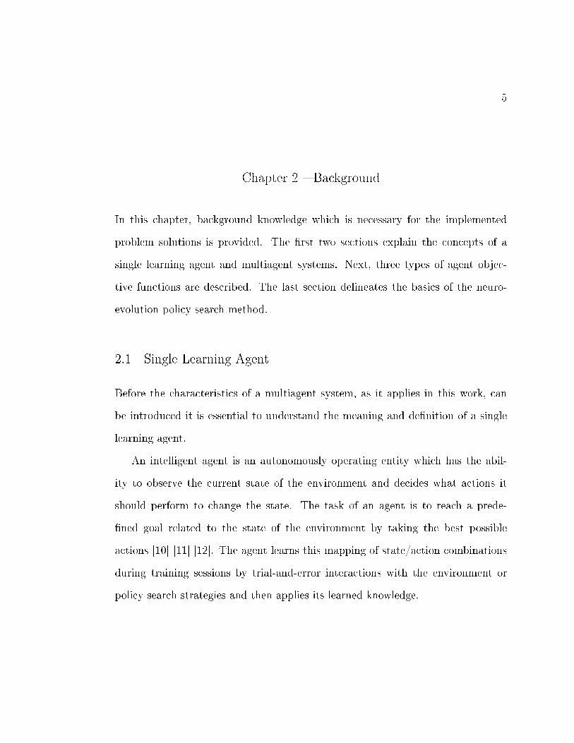
2.1 Single Learning Agent
Before the characteristics of a multiagent system, as it applies in this work, can
be introduced it is essential to understand the meaning and de�nition of a single
learning agent.
An intelligent agent is an autonomously operating entity which has the abil-
ity to observe the current state of the environment and decides what actions it
should perform to change the state. The task of an agent is to reach a prede-
�ned goal related to the state of the environment by taking the best possible
actions [10] [11] [12]. The agent learns this mapping of state/action combinations
during training sessions by trial-and-error interactions with the environment or
policy search strategies and then applies its learned knowledge.

6
Agent Environment
Reward
Action
Sensors
Effectors
Policy
State
Figure 2.1: A single agent framework where an agent observes the state of theenvironment and performs an action depending on its policy. The reward signalapplies to rank the agent's policy.
While the agent learns the mapping of state/action combinations it receives a
reward signal for chosen actions in a certain state depending on the performance
measurement. Di�erent types of performance measurement can be utilized to
compute this reinforcement signal. These objective functions are described later
in this chapter. A general single agent framework is illustrated in Figure 2.1
where the agent receives the state information of the environment via sensors,
chooses an action depending on its current policy and performs this action via its
e�ectors. The reward signal evaluates the policy depending on the current state
of the environment.

7
2.2 Multiagent Systems
In large and complex systems it is reasonable to use a number of individual units to
achieve a globally de�ned goal. This leads to the de�nition of a multiagent system
(MAS) where multiple intelligent agents interact together in the environment. It
is characterized in a way that a collective of agents is self-organized in searching
for the best system solution. However, one single agent in a MAS usually does not
have a view of the total environment [12] [13]. The agents in a MAS can either
learn with a shared policy or learn individual control policies to achieve a globally
de�ned goal. To reach this global goal, communication among agents is sometimes
necessary. However, in this work the agents are not able to communicate with each
other to transfer information about the world.
Large multiagent system where each agent learns an individual control policy
can be more e�cient, more robust and more �exible than a multiagent system with
a shared policy [14] because each agent is able to take actions which are best for
its own characteristics and the overall system performance.
A common example for a multiagent system is the 'predator-prey problem'
where a number of predator agents have the goal to capture a prey agent by
surrounding it [15]. Other examples are mobile sensor networks [16] or 'Rover-
Problems' where a collective of rovers works together and observes the environment
to achieve a globally de�ned goal [17] [18] [19].

8
2.3 Objective Functions in a Multiagent System
Evaluating the system performance in a multiagent system is an important part of
designing learning algorithms. The objective function calculates the quality of the
whole system at a certain time. A system is usually evaluated either at the end of
a learning episode or after a certain number of time steps. In this section, three
types of objective functions based on the theory of collectives [20] are described.
First, the global objective functionG(z) is explained. This function depends
on the state of the full system (e.g. position of all sources and agents and their
in�uence on the system) indicated by z. The goal of the agents is to maximize
G(z) in the system. For performance measurement, the global objective function
indicates the quality of the overall system. Additionally, this objective function
can be used to evaluate the learning of a shared policy or of individual agent
policies. However, the idea of applying the global objective function as a reward
signal is often part of a single agent system or a small multiagent system where a
shared policy is learned [21]. Previous research shows that in the case of evaluating
individual policies, the global objective function does not work as well as the other
objective functions because even non-optimal agent behavior can be rewarded if
other agents in the environment perform well. Also, the opposite case can occur
when an agent performs well but all the other agents do not. The overall reward
in this case will be low [17].

9
To solve this problem, the di�erence objective function can be applied.
This objective function is commonly used in multiagent domains to evaluate the
learning of individual policies. It is abstractly de�ned by the following equation:
Di(z) ≡ G(z)−G(z−i) (2.1)
Where i indexes agents and z−i contains the system state without the in�uence of
agent i. Usually this objective function has a higher sensitivity, meaning that an
agent gets more information about the performance of its behavior in the environ-
ment. In this way the di�erence equation indicates the direct in�uence of agent i
to the global objective G(z) [17] [20].
The third objective function used in this work is the local objective function
Li(z). It is also commonly used for evaluating the learning of individual agent
policies in a multiagent domain. In this work, the local objective depends only on
the in�uence of agent i. All other agents have no impact on the current state of the
environment. The local objective is abstractly de�ned by the following equation
where G(z+i) is the global objective function in which only agent i has an in�uence
on the environment.
Li(z) ≡ G(z+i) (2.2)
These objective functions are utilized in this work to evaluate the performance
of agents in a multiagent system.
10
2.4 Neuro-Evolution
In continuous, non-linear control tasks like pole balancing [22] [23], rocket control
[24] or robot navigation [19] [25], arti�cial neural networks achieve good results.
With arti�cial neural networks, there is the advantage of representing a continuous
state and action space compared to other reinforcement learning methods (e.g. Q-
learning, look-up tables [10]) which are usually used for a discrete state and action
space.
The neuro-evolution method combines these arti�cial neural networks and evo-
lutionary algorithms to learn a policy without explicit targets. This means that no
supervised learning applies. Instead, neuro-evolution explores the space of neural
network weights which leads to a good control policy and maximizes an objective
function. With the algorithm used in this work, the connection weights of the
neural networks are modi�ed to �nd good parameters [19] [26] [27] [28].
2.4.1 Arti�cial Neural Networks
Arti�cial neural networks are able to represent most continuous functions as a
function approximation [11]. They consist of several units (neurons) connected by
links where each link is weighted with a parameter w [29]. Units receiving the
information directly from the environment are named as input units xi. If these
input units are connected directly to the output units yo, the network is called a
single layer network. When there is another layer between the input layer and the
output layer the network is called a multilayer network. In a network like this, the

11
Figure 2.2: Topology of a two-layer, feed forward network with i input units, jhidden units, o output units and weighted links with weight factors wi,j and wj,o.
input units are connected to hidden units hj. These hidden units are either linked
to other hidden units if more layers exist or to output units. In this work a two-
layer feed forward network is used. Such a network has one layer of hidden units
connected to the output layer and all the links between layers are unidirectional
without any recursive cycles (See Figure 2.2).
The following equations explain how to compute the output of a processing
unit with a given input vector, bias and weight factors (See Figure 2.3). Typically,
the input signals xi are real numbers in the range [0.0, 1.0]. If the input signals are
outside of this range, normalization by compression is usually necessary [30].

12
weighted inputs activation function
Figure 2.3: Output computation of a processing unit with weighted inputs andbias by an activation function.
First, a sum over all the weighted inputs of a processing unit plus a weighted
bias value is calculated (See Equation 2.3). The bias b in this equation is used as
an o�set for the activation function. Commonly, it is set to 1.0 and weighted by a
separate weight factor.
sj = wb · b+∑
i
wi,j · xi (2.3)
This sum sj applies as the input of an activation function. Di�erent types of
functions are possible (See Figure 2.4). These activation functions calculate the
output of a processing. In this work, the sigmoid function applies as an activation
function. The output range of most activation functions is bounded between 0.0
(inactive) and 1.0 (active). Either a hard threshold like the threshold function or
a soft threshold like the linear or the sigmoid activation function is possible.

13
Figure 2.4: Activation functions: (left) threshold function (Equation 2.4), (center)partial linear function (Equation 2.5), (right) sigmoid function (Equation 2.6)
f(x) =
1 x ≥ 0
0 x < 0
(2.4)
f(x) =
1 x ≥ 1
2
x+1
2−1
2< x <
1
2
0 x ≤ −1
2
(2.5)
f(x) =1
1 + e−x(2.6)
14
Population of Neural Networks
Agent with current Network
Environment
State
Action
Fitness
Figure 2.5: Agent interacting with the environment by observing the state and per-forming an action. An evolutionary algorithm applies to select a network from thenetwork population. The �tness of the current network is ranked by an objectivefunction with regard to the population.
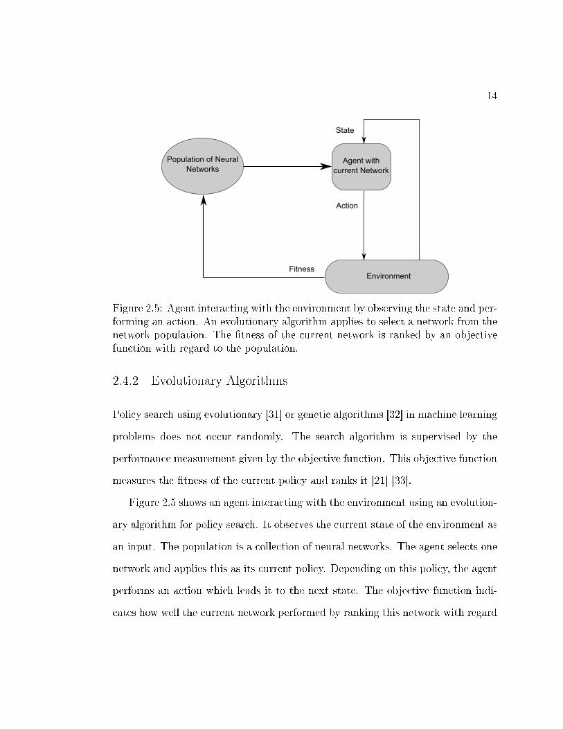
2.4.2 Evolutionary Algorithms
Policy search using evolutionary [31] or genetic algorithms [32] in machine learning
problems does not occur randomly. The search algorithm is supervised by the
performance measurement given by the objective function. This objective function
measures the �tness of the current policy and ranks it [21] [33].
Figure 2.5 shows an agent interacting with the environment using an evolution-
ary algorithm for policy search. It observes the current state of the environment as
an input. The population is a collection of neural networks. The agent selects one
network and applies this as its current policy. Depending on this policy, the agent
performs an action which leads it to the next state. The objective function indi-
cates how well the current network performed by ranking this network with regard

15
to the population of networks. Selecting the current network from the population
occurs with an ε-greedy evolutionary algorithm (See Algorithm 2.1) [19] [34]. Ei-
ther each agent holds its own population of individual neural network parameters
or a commonly shared network population is used. By the process of selecting
the highest ranked network from the population and mutation of the neural net-
work parameters to create new individuals, the evolutionary algorithm leads to a
population of neural networks which better suits the environment than the initial
population in the beginning of the search process.
Algorithm 2.1: ε-greedy Evolutionary Algorithm to determine Neural Net-work weights
1Initialize N networks in the population2for e = 1 to EPISODES do3Select Ncurrent from the population4with probability ε: Ncurrent ← Nrandom
5with probability 1− ε: Ncurrent ← Nbest
6Modify connection weights of Ncurrent
7Use Ncurrent for controlling8Evaluate Ncurrent at the end of an episode based on objective function
(G, D or L)9Replace Nworst with Ncurrent
10end

16
First, all N networks in the population are initialized with random values. In
this work, selection of the current network occurs at the beginning of a learning
episode. For selecting the current network, ε-greedy selection is used meaning that
with a probability of ε = 10% a random network from the network population
is chosen. The remaining 90% of the time, the best ranked network from the
population. In this way, neural networks which performed well previously are likely
to be selected, while still allowing lower ranked policies from the population to be
chosen and mutated to �nd superior policies. After selecting the current network,
the connection weight are modi�ed by mutation. For modifying, a random number
is added to each weight factor. This mutated current network is then used for
extent of the learning episode. After an episode of several time steps, the network
is ranked with an objective function and replaces the worst ranked network in
the network population. This approach leads to a converged population of neural
networks. Instead of ranking the neural network at the end of a learning episode, it
is also possible to rank the network more than one time during a learning episode.
The evolutionary algorithm in this work applies either for learning a full-system
shared policy or individual agent policies [35]. Using a full-system shared policy
implies that the individual actions of each agent are controlled by a common pol-
icy. For performance measurement and evaluation, the global objective function
G(z) is utilized. Learning individual policies means that each agent holds its own
population of neural networks and evolves its own individual policy. In this case,
all the three types of objective functions described in Section 2.3 will be applied
for evaluation. This enables a comparison between these evaluation methods.

17
Chapter 3 � Problem Domain
A description of the problem to solve is provided in this chapter. This conveys a
way of modeling the world with sources of information and sensor agents. Addi-
tionally, a de�nition of an agent in this domain is given. For measuring the full
system performance and for policy evaluation, the global objective function is de-
scribed in detail, including a method to compute the relationships among agents
and sources in the world which leads to the de�nition of the source coverage.
3.1 Problem Description
The world in this problem domain consists of a two dimensional plane area where
sources of information and sensor agents are randomly distributed (See Figure 3.1).
It is also possible to expand this problem to a 3-D world by adding another di-
mension. For a faster calculation of results, only the two dimensional plane area
applies.
The sources of information in the world are de�ned by individual information
type strengths. In a real world application the information types can be for example
temperature or pressure. Sources have the ability to o�er more than one type
of information. The location of these sources in the world is on �xed points,
initialized randomly at the beginning of an experiment. The sensor agents in this

18
source
agent
Figure 3.1: Two dimensional plane area with randomly distributed sources andagents constrained by a border on all edges.
domain are able to sense these di�erent information types and use the information
for computations. How well an agent can sense a certain type of information is
indicated by its individual type e�ciencies. As with sources, it is also possible that
a sensor agent is able to sense more than one type of information with variable
e�ciencies. In contrast to the sources, the agents can move in the world to look for
good locations or in case of sensor failures change their current position to recover
system performance.
19
010
2030
40
0
10
20
30
400
0.2
0.4
0.6
0.8
1
x
Drop off function
y
f(x,
y)
010
2030
40
010
2030
40−1
−0.8
−0.6
−0.4
−0.2
0
x
Drop off function
y
f(x,
y)
Figure 3.2: Drop o� functions: (left) source drop o� function (+1.0|100.0|5.0|0.5)(right) agent drop o� function (−1.0|20.0|5.0|0.5)
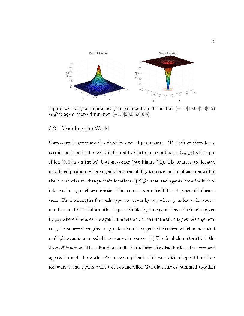
3.2 Modeling the World
Sources and agents are described by several parameters. (1) Each of them has a
certain position in the world indicated by Cartesian coordinates (x0, y0) where po-
sition (0, 0) is on the left bottom corner (See Figure 3.1). The sources are located
on a �xed position, where agents have the ability to move on the plane area within
the boundaries to change their locations. (2) Sources and agents have individual
information type characteristic. The sources can o�er di�erent types of informa-
tion. Their strengths for each type are given by νj,t where j indexes the source
numbers and t the information types. Similarly, the agents have e�ciencies given
by µi,t where i indexes the agent numbers and t the information types. As a general
rule, the source strengths are greater than the agent e�ciencies, which means that
multiple agents are needed to cover each source. (3) The �nal characteristic is the
drop o� function. These functions indicate the intensity distribution of sources and
agents through the world. As an assumption in this work, the drop o� functions
for sources and agents consist of two modi�ed Gaussian curves, summed together

20
(See Equation 3.1). Other types of intensity distributions are also possible but
have not been investigated in this work.
fs(x, y, x0, y0) = a
(η · e−
(x−x0)2+(y−y0)2
λW + (1− η) · e−(x−x0)2+(y−y0)2
λN
)fa(x, y, x0, y0) = a
(η · e−
(x−x0)2+(y−y0)2
λW + (1− η) · e−(x−x0)2+(y−y0)2
λN
)(3.1)
In these equations a is the amplitude. For sources a ∈ R+ and for agents
a ∈ R−. The factor η weights the two terms. One term indicates the wide region
and the other the nearby region of the intensity distribution. It is in a range of
0.0 ≤ η ≤ 1.0. The two range factors λW and λN specify the wide range and
the nearby range. A drop o� function is de�ned by a given quadruple (See Equa-
tion 3.2). As an example, Figure 3.2 shows the drop o� functions for a source and
for an agent.
(a|λW |λN |η) (3.2)
3.3 Agent De�nition
The agents in this domain operate as sensor units for special types of informa-
tion. As mentioned, a sensing unit can sense more than one type of information.
Additionally, each agent is also able to sense the location of sources in the world.
This information applies as a representation of the current state of an agent in the
environment. Two di�erent solution strategies are described further which di�er
in the way of sensing and representing the state.

21
Before an action can be performed, a mapping of state/action is essential. This
mapping occurs with an arti�cial neural network where the state information is
utilized as input of the network and the output represents the action to perform.
As described, an agent is able to move in the world to �nd a good location.
The direction of this movement depends on the chosen action. As with the repre-
sentation of the state, the two solution strategies di�er in the way of representing
the action to perform. These di�erences are described later in this thesis.
Learning the mapping of state/action occurs by training the neural network.
This training of neural networks takes place with an evolutionary algorithm. The
goal is to converge a population of neural networks toward a good solution. In this
way, a neural network can be found which suits best to the environment and the
agent's objective. In a multiagent system it is possible that either all agents share
a control policy for the mapping or each agent has its individual control policy.
3.4 Source Coverage
The coverage of a source for a certain type of information depends on the infor-
mation type strengths νj,t and the relationship among this source and the agents
indicated by ν ′j,t (See Algorithm 3.1). The calculation of this relationship is given in
Algorithm 3.2 and explained by an example. A coverage with a value of 0.0 means
that no agent is related to this type of information the source o�ers, whereas a
value of 100.0 means that an information type of a source is completely covered
by agents in the world.

22
Algorithm 3.1: Calculation of the Information type Coverage for eachSource
1for j = 1 to SOURCES do2for t = 1 to TY PES do
3Cj,t ←νj,t − ν ′j,tνj,t
· 100.0;
4end
5end
The example given in Figure 3.3 shows how the calculation of the relationship
works. In the top picture, a source drop o� function is given. The source has
an information type strength of +1.0 at position (20.0, 20.0). The picture in the
middle shows the drop o� function of an agent. Its information type e�ciency
at position (20.0, 20.0) is at −0.4361. The resultant shape of the source drop o�
function is given in the bottom picture, where the related information type strength
now has the value of +0.5638. This calculation is given in Algorithm 3.2, where
µi,t · fa(xj, yj, xi, yi) computes how agent i is related to the strengths of source j,
depending on relative position and information type e�ciencies.
Algorithm 3.2: Relationship among Agents and Sources for all types ofInformation
1for j = 1 to SOURCES do2for t = 1 to TY PES do3ν ′j,t ← νj,t +
∑i
(µi,t · fa(xj, yj, xi, yi));
4if ν ′j,t < 0 then5ν ′j,t ← 0;6end
7end
8end

23
010
2030
40
0
10
20
30
400
0.2
0.4
0.6
0.8
1
x
Source at postion (20,20)
y
f s(x,y
)
010
2030
40
0
10
20
30
40−1
−0.8
−0.6
−0.4
−0.2
0
x
Agent at position (18,18)
y
f a(x,y
)
010
2030
40
0
10
20
30
400
0.2
0.4
0.6
0.8
x
Related Source Strength
y
f s(x,y
)
Figure 3.3: Example for the relationship of an agent to a source. This relationshipis indicated by a lower amplitude of the source drop o� function in the bottompicture.

24
3.5 Global Objective Function
The global objective function G(z) measures the full system performance. It ap-
plies to both solution strategies used in this work, which are described in Chapters
4 and 5. In this way the results of both strategies can be compared. However, the
solution strategy in a partially observable world is more realistic than the strategy
in a fully observable world. The di�erence between these two solution strategies
will be described further.
The equation for the global objective function is given in Equation 3.3. In this
equation the sum over all coverage values (See Algorithm 3.1) is calculated and
divided by the product of the amount of sources j and types t in the world to make
sure that the values of the global objective are in a range between 0.0 and 100.0
for a better comparison of the results.
G(z) =
∑j
∑t
Cj,t
j · t, {G(z) ∈ R|0.0 ≤ G(z) ≤ 100.0} (3.3)
Additionally, the global objective function applies as one possibility of evalu-
ating the behavior of agents in the world.
25
Chapter 4 � Fully Observable World
The strategy described in this chapter involves a fully observable world, meaning
that all agents can see the relationships between agents and sources. Despite the
fact that this is a non-realistic situation, this method allows the evaluation of the
system performance for a solution strategy, as described in Chapter 5. Additionally
in this chapter, the agent de�nition from Section 3.3 is described in detail for the
solution strategy in a fully observable world.
4.1 Agent Sensing
In a fully observable world, the intensity of sources is related to agents in the world.
A highly related source is indicated by a relatively low intensity distribution. The
agents are able to sense these relationships for state representation.
Representing the current state, an agent measures the information value at
its position (xk, yk) and in steps of ϕ = 45◦ with a certain distance at position
(x′k, y′k) where k indexes the step numbers (See Figure 4.1). With these values,
the information changes ∆ϕ are calculated (See Algorithm 4.1) and apply as a
representation for the current state of the environment.

26
Figure 4.1: Sensing in a fully observable word. The agent senses the informationvalue at its current position (xk, yk) and around its position in steps of ϕ = 45◦
(x′k, y′k) to calculate the information change values ∆ϕ.
To compute these information changes, the agent deactivates itself. In this
way the agent gets only the information of sources related to all other agents.
The algorithm given in Algorithm 4.1 explains the calculation of the information
change values where I(x, y, µi,t) is the function to compute the information value at
a certain position. This calculation is given in Algorithm 4.2, where the intensity
of source j, depending on the drop o� characteristic (See Equation 3.1) is weighted
with the related type strengths ν ′j,t. For computing the amount of information I
an agent can receive at this location, the value is also weighted with its own type
e�ciencies µi,t.

27
Algorithm 4.1: Fully Observable World: Get Information changes for eachAgent
1for i = 1 to AGENTS do2deactivate agent i for in�uence calculation;3compute related source strengths ;4Vk ← I(xk(i), yk(i), µi,t);5for ϕ = 0◦ to 360◦; ϕ+ = 45◦ do
6x′k(i)← xk(i) + 0.25 cos(ϕ · π180◦
);
7y′k(i)← yk(i) + 0.25 sin(ϕ · π180◦
);
8V ← I(x′k(i), y′k(i), µi,t);9∆ϕ ← V − Vk;10end11activate agent i;12∆i,ϕ ← ∆ϕ;13end
Algorithm 4.2: Fully Observable World: Information Value for Agent i ata certain Position weighted with its own E�ciencies. I(x, y, µi,t)
Input: x,y, µi,t
1for t = 1 to TY PES do2Vt ←
∑j
(ν ′j,t · fs(x, y, x0(j), y0(j)));
3end4I ←
∑t
(µi,t · Vt);
Result: I

28
4.2 Agent Mapping
For mapping of state/action combinations, an arti�cial neural network is utilized.
This network consists of 8 input units, 16 hidden units and 2 output units.
With the current state ∆ of an agent, the action to choose is calculated by the
neural network. First, the information changes have to be prepared to be used as
inputs of the neural network. Hence, a dynamic linear compression is conducted
(See Algorithm 4.3). In this way, the information change values are always repre-
sented in a range between 0.0 and 1.0, where 0.0 is the minimal information change
value and 1.0 the maximal information change value in a certain time step.
The output of the neural network applies to represent the action to choose. It
consists of two values, O1 and O2 in a range between 0.0 and 1.0.
Algorithm 4.3: Fully Observable World: Dynamic Input Compression forNeural Network
1for i = 1 to AGENTS do2get information_changes of agent i ;3min← min(∆i,ϕ);4max← max(∆i,ϕ);5for f = 1 to 8 do6ϕ← (1− f)45◦;
7inputi,f ←∆i,ϕ −minmax−min
;
8end
9end

29
4.3 Agent Action
In this solution strategy, the output of the neural network directly indicates the
direction to move (See Equation 4.1) where (xk, yk) is the current position of the
agent and (xk+1, yk+1) the new position after moving. The step_size parameter
in this work is set to 0.25. With this representation of the neural network output
as an action, an agent is able to move in all directions.
xk+1 = xk + step_size (O1 − 0.5)
yk+1 = yk + step_size (O2 − 0.5) (4.1)
4.4 Agent Learning and Objective
The global objective function described in Section 3.5 applies as an objective func-
tion to evaluate the behavior of the agents. In a fully observable world, only a
shared policy for all agents is developed. In this case, the population consists of
N = 50 neural networks. The results of this solution strategy are compared later
in this work with the results of the partially observable world, which is described
in Chapter 5. For this reason, the experiment con�gurations must be equal for
both solution strategies. These con�gurations are explained further in Section 6.1.
30
Chapter 5 � Partially Observable World
This chapter explains another method for solving the problem. Unlike the fully
observable world, which is non-realistic, in this representation the sensor agents can
not sense the relationships among agents and sources. However, these relationships
are still utilized for computing the objective functions to evaluate the behavior of
agents. Like in the chapter of the fully observable world, the agent de�nition from
Section 3.3 is described in detail for a partially observable world.
5.1 Agent Sensing
The world around the agent is broken up into four sensing quadrants q. For each
quadrant, the total sensing information is separated into (1) sensing of sources
Si,t(q) and (2) sensing of other agentsAi,t(q) where t indexes the type of information
and i the agent, sensing these information (See Figure 5.1).
The information gathered for Si,t(q) consist of the information type strength
νj,t of source j located in quadrant q, the maximum information type strength,
where all source strengths are considered, and the distance δ between the agent
and this source. Similarly, for calculating the information gathered for Ai,t(q),
the information type e�ciency µa,t of an agent a located in quadrant q applies.
Computing the distance, the Euclidean norm is used with a constant added to

31
source
agent
agent sensor
source sensor
q1q2
q4q3
Figure 5.1: Sensing structure of agent i in a partially observable world. Theinformation is separated into four quadrants. For each quadrant there is a sensorfor agent-information and source-information.
prevent singularities when an agent is close to a source or another agent. However,
other types of distance metric could also be used but have not been investigated.
The total information of sources and agents in a quadrant is also separated into
the di�erent possible types of information t. Unlike in a fully observable world, the
information type e�ciency of agent i is not included to the calculation. In addition
of controlling the movement of the agent, the agent's goal is to learn which type
of information is interesting for this agent by �ltering the sensed information.
δi,j = ||i− j||+ 1.0
Si,t(q) =∑j∈q
νj,t
max(ν) · δi,j(5.1)
δi,a = ||i− a||+ 1.0
Ai,t(q) =∑a∈q
µa,t
max(µ) · δi,a(5.2)

32
SOURCES AGENTS
Figure 5.2: Linear cut o� functions: (left) for Si,t(q) (right) for Ai,t(q). Theseguarantee that the values are within a range between 0.0 and 1.0
To guarantee that the values of the Si,t(q) and Ai,t(q) are in a range between
0.0 and 1.0, linear cut o� functions are utilized (See Figure 5.2). Unlike in the
fully observable world, the cut o� compression does not occur dynamically. The
slope of these cut o� functions only depends on the total number of sources and
agents in the world.
Si,t(q) =
0.0 Si,t(q) ≤ 0.0
Si,t(q)
SOURCES0.0 < Si,t(q) < SOURCES
1.0 Si,t ≥ 1.0
(5.3)
Ai,t(q) =
0.0 Ai,t(q) ≤ 0.0
Ai,t(q)
AGENTS0.0 < Ai,t(q) < AGENTS
1.0 Ai,t ≥ 1.0
(5.4)

33
5.2 Agent Mapping
With the two parameters Si,t(q) and Ai,t(q), the current state of agent i is com-
pletely described. However, the mapping of state/action combinations takes place
indirectly. First, agent i assigns a quality value for each quadrant q depending on
the state information. After this assignment, these quality values Qi(q) are used
to select a quadrant for the action. Two methods are implemented for this quality
value assignment.
• Deterministic Method without learning
• Arti�cial Neural Networks with learning by Neuro-Evolution
5.2.1 Agent Mapping using Deterministic Method
The mapping with a deterministic quality value assignment without learning can
be calculated using the linear function:
Qi(q) =∑
t
(Si,t(q)− Ai,t(q)) (5.5)
The quality has the highest value if there is a low value of total agent informa-
tion and a high value of total source information in a quadrant. This quadrant is
more important for an agent to move into than a quadrant with a high value of
total agent information and low total source information (See Figure 5.3). In this
way, the agents are forced to move into a direction, where the chance of �nding

34
0
0.2
0.4
0.6
0.8
1
0
0.2
0.4
0.6
0.8
1−1
−0.5
0
0.5
1
S(q)
Deterministic Policy (1 TYPE)
A(q)
Q(q
)
Figure 5.3: Linear, deterministic quality assignment for single type of information.The maximum quality value is assigned if the amount of source information ismaximum and the amount of agent information is minimum.
under-covered sources is highest. The deterministic assignment applies as an hand
coded policy to be compared with the learning policies in this work. The experi-
ments will show the need of learning individual policies instead of a deterministic.
5.2.2 Agent Mapping using Arti�cial Neural Networks
Here, the quality value in a quadrant is assigned by an arti�cial neural network. For
this task, a two-layer, feed forward, sigmoid activated network with (2 · TY PES)
input units, 16 hidden units and 1 output unit is utilized. Former experiments in
this work showed that a number of 16 hidden units is enough if the world consists of
three or less types of information. If there are more types of information available,
the number of hidden units has to be increased.

35
For each quadrant, the neural network simulates the output which is used as
a quality value Qi(q) for this quadrant. The inputs of the neural network are
the total source information Si,t(q) and the total agent information Ai,t(q) in the
current quadrant q under investigation, separated into the information types.
5.3 Agent Action
After the quality assignment for the quadrants, the quadrant with the highest
quality is chosen for the action. The angle of the direction to move is in the middle
of this quadrant. Equation 5.6 calculates this angle depending on the quadrant
with the highest quality. The number of QUADRANTS is set to 4.
ϕ =360◦ · q|max Q(q)
QUADRANTS+
360◦
2 ·QUADRANTS(5.6)
With this angle, the new position of the agent is computed. A step_size
of 0.25 is used in this work. In Equation 5.7, the new coordinates (xk+1, yk+1)
are calculated depending on the current position (xk, yk), the step_size and the
direction to move, indicated by ϕ. The step numbers are indexed by k.
xk+1 = xk + step_size · cos(ϕ · π180◦
)
yk+1 = yk + step_size · sin(ϕ · π180◦
)
(5.7)

36
5.4 Agent Learning and Objectives
Training the neural networks occurs with a neuro-evolution search algorithm (See Al-
gorithm 2.1). In addition to a shared policy, like it applies in a fully observable
world, individual control policies are evolved. In this case, each agent holds its own
population of neural networks and develops its own policy in respective of its char-
acteristic. For the development of a shared policy, a population of N = 50 neural
networks is utilized, whereas for individual policies, each agent holds a population
of N = 20 neural networks.
A performance evaluation of the current used neural network takes only place
once at the end of an learning episode. The shared policy is only evaluated with
the global objective, whereas the individual policies are evaluated in three di�erent
ways. As with the shared policy, the global objective function applies. In addition
to this evaluation method, the di�erence and local objective functions are utilized.
• Global Objective Function
The global objective G(z) given in Equation 3.3 re�ects the overall system
performance regarding the behavior of all sensor agents. The goal of the
agents is to maximize this objective. It is used for ranking the performance of
a shared policy and the performance of individual policies in this multiagent
system.

37
• Di�erence Objective Function
The di�erence objective Di(z) given in Equation 2.1 is only used for ranking
the learning of an individual policy in this multiagent system. For calculating
G(z−i), used in the di�erence objective function, agent i is deactivated when
computing the related type strengths ν ′j,t of the sources (See Algorithm 3.2).
In this way, agent i has no impact on this calculation. After the calculation
agent i is reactivated.
• Local Objective Function
The local objective Li(z) given in Equation 2.2 applies only for ranking the
learning of an individual policy in this multiagent system. For calculating
Li(z) all the agents except agent i are deactivated when calculating ν ′j,t of
the sources (See Algorithm 3.2). In this way, these values depend only on the
relationship of agent i. After this process, all the other agents are reactivated.

38
Chapter 6 � Experiments
First, the experiments chapter gives an overview about experiment de�nition with
all necessary con�gurations. Following, several experiments were designed to es-
timate the behavior of agents under certain circumstances. Finally, the results of
the experiments are discussed.
• World with Single Type of Information: The agents must learn to �nd
a source of information for a good system coverage in a world with one type
of information.
• World with Multiple Types of Information: This experiment builds
on the �rst experiment, requiring that the agents must learn learn to �lter
information depending on their individual con�gurations in a world with
three types of information.
• System Robustness: In a partially observable world with multiple types of
information, agent failures were simulated. Other agents in the world must
recover system performance.
• Policy Recon�guration: In a partially observable world with multiple
types of information, agents were removed from the system or added to the
system. The agents must recon�gure their individual policies to perform well
under the new circumstances.

39
6.1 Experiment De�nition
The con�gurations for the experiments include parameters about the world with
sources and agents, training con�gurations of the neuro-evolution algorithm and
experiment con�gurations.
• Plane Area
The two dimensional plane area had a size of 40.0 × 40.0. In the beginning
of each episode, the location of sources and the start positions of agents were
randomly distributed. However, the minimum distance between sources was
set to 5.0 to make sure that sources do not have an in�uence on each other.
Without this con�nement it can also be possible that an agent �nds a good
location between sources. But in this work, the goal of the agents should be
to stay directly on a certain source.
• Source Parameters
The information type strength values νj,t of sources were randomly initialized
in a range of 3.0 to 6.0. For multi-type experiments it was also possible that
a certain type strength was set to 0.0, meaning that the source does not
o�er this type of information. For computing in a fully observable world the
parameters of the source drop o� function were set to (+1.0|160.0|4.0|0.5).
However, these parameters have no use in the partially observable world.
With this high value for the wide range factor λW , a source has an in�uence
all over the world and the agents are able to sense the e�ect of sources from

40
each position. In a partially observable world this is not necessary because
the Euclidean distance between agents and sources is a criteria for the state
information.
• Agent Parameters Similarly, the information type e�ciency values µi,t of
agents were randomly initialized in a range of 1.0 to 2.0. For multi-type
experiments it was also possible that a certain type e�ciency was set to 0.0,
meaning that an agent is not able to measure this type of information. For
both solution strategies, the parameters of the agent drop o� function were
set to (−1.0|4.0|4.0|0.5). The range of the agent intensity is small compared
to the wide range of the sources, meaning that an agent has to be close to a
source for a good coverage.
• Training Con�gurations
In both strategies, the network population for learning a shared policy con-
sisted of N = 50 neural networks. In the partially observable world, learning
individual policies also applied. For these algorithms, a population of N = 20
was utilized. The neural network for the fully observable strategy consisted
of 8 input units, 16 hidden units and 2 output units. In the partially observ-
able world, the number of input units increases with the amount of possible
information types in the world. 2 · TY PES input units, 16 hidden units and
1 output unit were used. The number of hidden units must be increased if
more types of information are available. Experiments in this work showed
that a number of 16 hidden units with three types of information is su�cient.

41
• Experiment Con�gurations
In each training episode, the number of steps was set to 1500. With this
high number of steps it should be possible for all the agents to move to a
destination where the agent can improve the system performance. Ranking of
the current network occurred once at the end of an episode. The training with
a certain con�guration ended after 1500 episodes and was repeated 30 times
to average the results for analysis. The standard deviation of the results
is indicated by error bars. In the last 500 episodes, the ε-greedy network
selection method was turned o�. This means that training and evaluation
no longer take place and only the best ranked network is selected.
6.2 World with Single Type of Information
In this section the results of the experiments in a world with a single type of
information are shown and discussed. The parameters for source strengths and
agent e�ciencies are given in Table B.1.
As one result in a partially observable world, control surfaces of the neural
networks after training are shown in Figure 6.1. These surfaces are interpreted
as agent's policies. The x-axis and the y-axis are the inputs (Si(q), Ai(q)) of the
neural network and the z-axis is the output Qi(q). For comparison, four di�erent
surfaces are given. The top-left surface shows the shared policy trained with the
global objective function. As an example for individual policies trained with the
di�erence objective as an objective function, three di�erent surfaces are shown.

42
0
0.5
1
00.10.20.30.40.50.60.70.80.91
0
0.1
0.2
0.3
0.4
0.5
0.6
0.7
0.8
0.9
1
S(q)A(q)
Net Surface Shared Policy (1 TYPE)Q
(q)
0
0.5
1
00.10.20.30.40.50.60.70.80.91
0.92
0.93
0.94
0.95
0.96
0.97
0.98
0.99
1
S(q)A(q)
Net Surface Individual Policy of Agent 1 − trained on D (1 TYPE)
Q(q
)
0
0.5
1
00.20.40.60.81
0.85
0.9
0.95
1
S(q)A(q)
Net Surface Individual Policy of Agent 4 − trained on D (1 TYPE)
Q(q
)
0
0.5
1
00.10.20.30.40.50.60.70.80.91
0.7
0.75
0.8
0.85
0.9
0.95
1
S(q)A(q)
Net Surface Individual Policy of Agent 7 − trained on D (1 TYPE)
Q(q
)
Figure 6.1: Neural Network surfaces for a shared policy and three individual poli-cies trained with the di�erence objective function (5 sources and 15 agents): (left-top) shared policy, (right-top) individual policy with low e�ciency, (right-bottom)individual policy with medium e�ciency, (right-bottom) individual policy withhigh e�ciency
The quality value of the shared policy is at a maximum when there is a high
value of source and a low value of agent information in the quadrant. It decreases
if the value for agent information increases or if the value for source informa-
tion decreases. For analyzing the individual policies, it is necessary to look at
the e�ciencies of a certain agent. The three individual policies shown are poli-
cies of agents with a low e�ciency (Agent1;µ1,0 = 1.06629), a medium e�ciency
(Agent4;µ4,0 = 1.75392) and a high e�ciency (Agent7;µ7,0 = 1.96740).

43
The results show policies which di�er from the shared policy. An agent with
a low type e�ciency increases its quality value if the total agent information in a
quadrant increases. However, similar to the shared policy, the quality value also
increases if the total source information increases. Such an agent develops this kind
of policy, because even with a large amount of total agent and source information
in a quadrant this agent is still able to improve the system performance because
of its low e�ciency. Agents with a medium or a high e�ciency develop similar
control policies. For a smaller amount of total agent information in a quadrant,
these policies match with the shared policies. Di�erences appear if the total agent
information increases, whereas the total source information is at a high value. Both
policies then output a relatively high quality value compared to the shared policy.
In Figure 6.2 the movements of agents in a two dimensional world with a
single type of information and partial observability is shown. A con�guration of
10 agents and 5 sources was chosen to explain the behavior. To create a clear
result �gure, only every 20th step was plotted. In addition to the movements, the
�nal locations of agents and the position of sources are given in absolute Cartesian
coordinates. The �gure shows that all agents were able to move to a certain source
of information.
Interesting behavior of Agent3 can be contemplated. First this agent moved
toward Source2. As soon as more agents reach Source2 the source was over cov-
ered. In this case Agent3 decided to move toward Source0 to increase the system
performance.

44
0
5
10
15
20
25
30
35
40
0 5 10 15 20 25 30 35 40
y-A
xis
x-Axis
G(z) = 70.19
A0,(4.189 7.421)A1,(18.201 18.773)A2,(2.974 29.121)
A3,(14.455 26.608)A4,(14.017 14.147)A5,(18.046 18.811)A6,(14.162 26.695)A7,(18.232 18.798)
A8,(3.954 7.380)A9,(4.288 7.238)
S0,(14.317 26.599)S1,(13.909 14.153)S2,(18.134 18.791)
S3,(4.301 7.353)S4,(3.041 29.171)
Figure 6.2: Agents movement within a two dimensional, single information typeworld with 5 sources (S0...S4) and 10 agents (A0...A9) and partial observability.More agents are located on sources S2 and S3 because of their high type strength(See Table B.1).
A conclusion from this �gure is the fact that agents have the intention to move
toward the closest sources as long as this source is not over covered. This makes
sense in a way that the agents are not able to observe the whole world. To �nd
the best possible position an agent needs perfect visibility or should be able to
communicate with other agents to get more information about the world.

45
0 500 1000 15000
10
20
30
40
50
60
Episodes
G(z
)
Partially Observable Shared Policy (G)Partially Observable Shared Policy (HC)Fully Observable Shared Policy (G)
Figure 6.3: Results in a world with a single type of information for a con�gurationof 10 agents and 5 sources. The graphs show the development of shared policiescompared to a hand coded policy in a partially observable world. After 1000episodes the ε-greedy network selection is set to 0% meaning that the best rankednetwork is used all the time.
The training results given in Figures 6.3, 6.4 and Figures 6.5, 6.6 show the
development of the shared and individual policies applied in this work. As a mea-
surement for the system performance, the global objective G(z) as described in
Equation 3.3 is plotted over the number of episodes where error bars indicate the
standard deviation of the data after averaging. As an example, two di�erent con-
�gurations (10 agents/5 sources and 20 agents/5 sources) are used. The e�ciencies
and strengths are the same within each con�guration. In this way a comparison
between the di�erent strategies and objective functions is valid.

46
0 500 1000 15000
10
20
30
40
50
60
Episodes
G(z
)
Partially Observable Individual Policy (D)Partially Observable Individual Policy (L)Partially Observable Individual Policy (G)Random
Figure 6.4: Results in a world with a single type of information for a con�gurationof 10 agents and 5 sources. The graphs show the development of individual policiesin a partially observable world. After 1000 episodes the ε-greedy network selectionis set to 0% meaning that the best ranked network is used all the time.
For the development of a shared policy, the strategy in a partially observable
world was evaluated with the global objective (G) and compared to a deterministic,
hand coded solution (HC) and a learning policy evaluated with the global objective
function (G) in a fully observable world. These results are given in Figure 6.3
and 6.5. The individual policies apply only in the partially observable world.
Evaluation occurred in three di�erent ways; using the global (G), local (L) or
di�erence (D) objective functions. These results are given in Figure 6.4 and 6.6.
As a baseline for the performance, random behavior of individual policies was
included to the results. In this case, no evaluation of the current policies occurred.

47
0 500 1000 15000
10
20
30
40
50
60
70
80
90
100
Episodes
G(z
)
Partially Observable Shared Policy (G)Partially Observable Shared Policy (HC)Fully Observable Shared Policy (G)
Figure 6.5: Results in a world with a single type of information for a con�gurationof 20 agents and 5 sources. The graphs show the development of shared policiescompared to a hand coded policy in a partially observable world. After 1000episodes the ε-greedy network selection is set to 0% meaning that the best rankednetwork is used all the time.
All the applied policies for a di�erent number of agents are compared in Fig-
ure 6.7. In this �gure the maximum achieved values of G(z) are shown. The
number of agents for each con�guration increases with a step size of 5 agents start-
ing with 5 agents. The graph shows that in a partially observable world the shared
policy and the individual policy evaluated with the di�erence objective function
performed best.

48
0 500 1000 15000
10
20
30
40
50
60
70
80
90
100
Episodes
G(z
)
Partially Observable Individual Policy (D)Partially Observable Individual Policy (L)Partially Observable Individual Policy (G)Random
Figure 6.6: Results in a world with a single type of information for a con�gurationof 20 agents and 5 sources. The graphs show the development of individual policiesin a partially observable world. After 1000 episodes the ε-greedy network selectionis set to 0% meaning that the best ranked network is used all the time.
The results show that the learning procedure in a partially observable world
occurred faster than in a fully observable world. After approximately 700 training
episodes, the learning was converged. The reason for this behavior is the fact that
the neural network, applied in a partially observable world, consisted of two inputs,
whereas in a fully observable world eight inputs were used. In this case, it takes
longer to search in the space of weight factors.

49
5 10 15 20 25 300
10
20
30
40
50
60
70
80
90
100
Agents
max
G(z
)
Partially Observable Shared Policy (G)Partially Observable Shared Policy (HC)Partially Observable Individual Policy (D)Partially Observable Individual Policy (L)Partially Observable Individual Policy (G)Fully Observable Shared Policy (G)
Figure 6.7: Maximum achieved G(z) for the applied algorithms and �tness func-tions in a world with a single type of information. The number of agents startswith 5 agents and increases in steps of 5 agents to 30 agents
The best results in a world with a single type of information with partial ob-
servability can be achieved in two di�erent ways; either using a shared policy or
an individual policy evaluated with the di�erence objective function. With both
strategies the agents can learn to �nd a source of information independent of their
own information type e�ciency. These results are equivalent to using a hand coded
solution or a shared policy in a fully observable world meaning that in a world with
a single type of information a learning strategy is not inevitably necessary. The
need of individual policies will be shown in the next section where a world with
multiple types of information exists.

50
For all con�gurations of agents, the individual policies evaluated with the global
objective function performed worst. This conclusion makes sense because it is
possible good behavior of an individual agent was evaluated as being bad if all
the other agents performed suboptimal, or a bad behavior of an individual agent
was evaluated as good if all the other agents performed well. An agent gets little
feedback about the quality of its own behavior if the global objective function is
used for evaluating an individual policy.
The evaluation of individual policies with the local objective function performed
slightly better than the evaluation with the global objective function using indi-
vidual policies.
Figure 6.7 also shows that for a small amount of agents all the strategies per-
formed equally well. The reason for this behavior can be explained in a way that
with all these strategies it is possible for agents to �nd a good location but with a
small number of agents, an over coverage of sources does not often take place.
As a conclusion of these experiments, it is possible to control the agent's be-
havior using evolutionary algorithms based on neural networks. However, there is
no better behavior if individual control policies are applied. Although the agents
have only a partial observability of the world, they are able to perform equivalently
to agents operating in a fully observable world.

51
0
5
10
15
20
25
30
35
40
0 5 10 15 20 25 30 35 40
y-A
xis
x-Axis
G(z) = 63.31
A0,(21.125 33.407)A1,(21.127 33.539)A2,(32.797 17.421)A3,(32.576 17.312)A4,(14.767 23.353)A5,(21.413 33.008)A6,(28.567 2.276)
A7,(21.288 33.262)A8,(1.703 28.766)
A9,(14.957 23.347)S0,(21.257 33.374)S1,(14.852 23.388)S2,(32.718 17.437)S3,(28.438 2.265)S4,(1.680 28.800)
Figure 6.8: Agents movement within a two dimensional, multiple information typesworld with 5 sources (S0...S4) and 10 agents (A0...A9) and partial observability.The parameters are given in Table B.2.
6.3 World with Multiple Types of Information
Similar to the world with a single type information, the results of the experiments
in a world with multiple information types are shown and discussed in this section.
For these experiments a number of three types of information was chosen. The
parameters for source strengths and agent e�ciencies are given in Table B.2.

52
In a world with multiple types of information it is not possible to plot the
control surfaces of the neural networks for the policies in a partially observable
world because there were more than only two network inputs.
As in a world with a single type of information, the movements of the agents in a
partially observable world are given in Figure 6.8. This �gure shows a con�guration
of 5 sources and 10 agents moving in a world of multiple information types. The
individual control policies, as they were used for this result, were evaluated with
the di�erence objective function.
To explain the behavior of a certain agent it is necessary to take into consid-
eration the agents e�ciencies and sources strengths. The �gure shows that all
the agents learned to move toward a source. However, there is a di�erence in the
moving compared to the world with a single type of information. Now, the agents
are not moving straight toward the closest source. They learned to �lter the source
information. For example, Agent5 started close to Source3. It could sense this
source but it was not interested in the information types Source3 o�ered. A similar
behavior occurred when Agent5 was close to Source1. As a conclusion, the agents
are forced to �nd only sources with information types they are interested in. Non-
optimal results occurred if the behavior of Agent3 is examined. This agent moved
directly to Source2 because this source was the closest and it o�ered information
the agent was interested in. The problem with this result is that the system perfor-
mance could be increased if the agent was located at a di�erent source. Like before,
the problem is the partially observable world. To solve problems like this a perfect
visibility of the world or a communication between agents would be necessary.
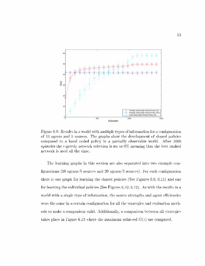
53
0 500 1000 15000
10
20
30
40
50
60
Episodes
G(z
)
Partially Observable Shared Policy (G)Partially Observable Shared Policy (HC)Fully Observable Shared Policy (G)
Figure 6.9: Results in a world with multiple types of information for a con�gurationof 10 agents and 5 sources. The graphs show the development of shared policiescompared to a hand coded policy in a partially observable world. After 1000episodes the ε-greedy network selection is set to 0% meaning that the best rankednetwork is used all the time.
The learning graphs in this section are also separated into two example con-
�gurations (10 agents/5 sources and 20 agents/5 sources). For each con�guration
there is one graph for learning the shared policies (See Figures 6.9, 6.11) and one
for learning the individual policies (See Figures 6.10, 6.12). As with the results in a
world with a single type of information, the source strengths and agent e�ciencies
were the same in a certain con�guration for all the strategies and evaluation meth-
ods to make a comparison valid. Additionally, a comparison between all strategies
takes place in Figure 6.13 where the maximum achieved G(z) are compared.

54
0 500 1000 15000
10
20
30
40
50
60
Episodes
G(z
)
Partially Observable Individual Policy (D)Partially Observable Individual Policy (L)Partially Observable Individual Policy (G)Random
Figure 6.10: Results in a world with multiple types of information for a con�gu-ration of 10 agents and 5 sources. The graphs show the development of individualpolicies in a partially observable world. After 1000 episodes the ε-greedy networkselection is set to 0% meaning that the best ranked network is used all the time.
The results show that in a world with multiple types of information the in-
dividual policies evaluated with the di�erence objective function performed best
for all con�gurations of agents. Individual policies are able to both select a direc-
tion to move and prepare the information which were important for an individual
agent meaning that the network worked like a kind of �lter. It was not possible to
achieve a similar behavior using a shared policy or using the simple, deterministic
hand coded policy. The more types of di�erent information are available the better
would these individual policies perform compared to the other policies.
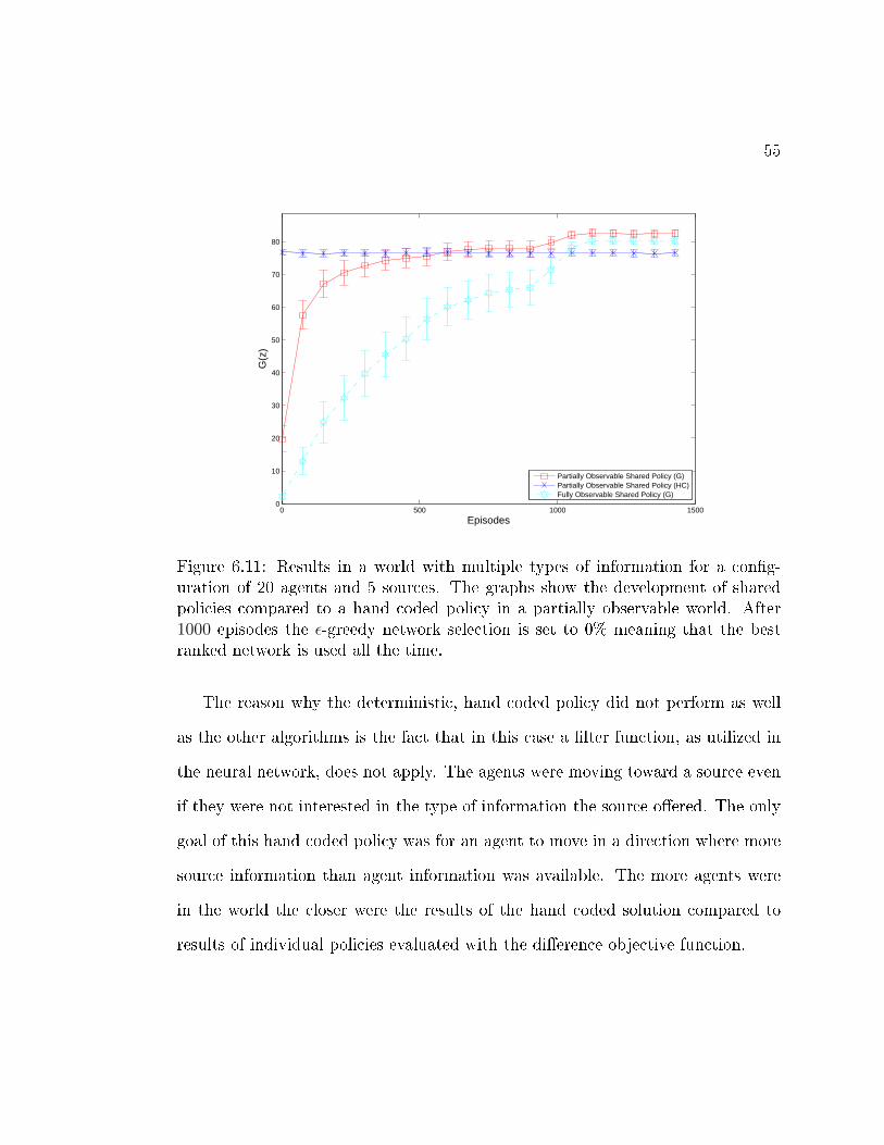
55
0 500 1000 15000
10
20
30
40
50
60
70
80
Episodes
G(z
)
Partially Observable Shared Policy (G)Partially Observable Shared Policy (HC)Fully Observable Shared Policy (G)
Figure 6.11: Results in a world with multiple types of information for a con�g-uration of 20 agents and 5 sources. The graphs show the development of sharedpolicies compared to a hand coded policy in a partially observable world. After1000 episodes the ε-greedy network selection is set to 0% meaning that the bestranked network is used all the time.
The reason why the deterministic, hand coded policy did not perform as well
as the other algorithms is the fact that in this case a �lter function, as utilized in
the neural network, does not apply. The agents were moving toward a source even
if they were not interested in the type of information the source o�ered. The only
goal of this hand coded policy was for an agent to move in a direction where more
source information than agent information was available. The more agents were
in the world the closer were the results of the hand coded solution compared to
results of individual policies evaluated with the di�erence objective function.
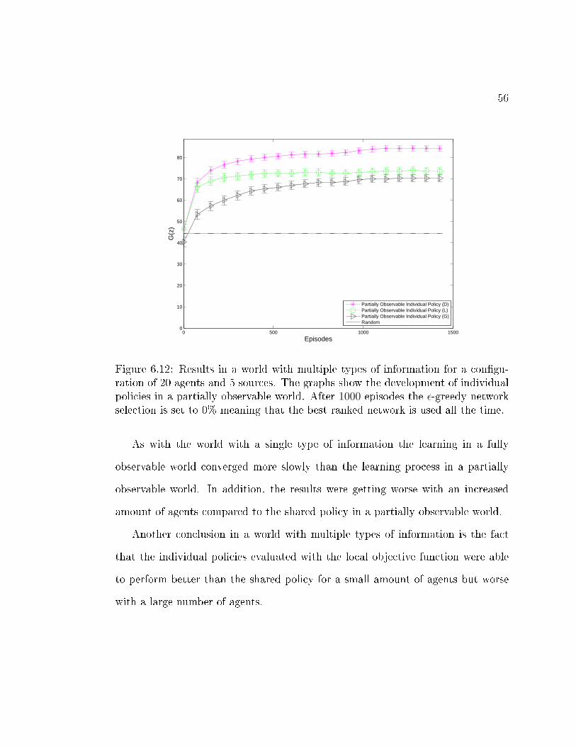
56
0 500 1000 15000
10
20
30
40
50
60
70
80
Episodes
G(z
)
Partially Observable Individual Policy (D)Partially Observable Individual Policy (L)Partially Observable Individual Policy (G)Random
Figure 6.12: Results in a world with multiple types of information for a con�gu-ration of 20 agents and 5 sources. The graphs show the development of individualpolicies in a partially observable world. After 1000 episodes the ε-greedy networkselection is set to 0% meaning that the best ranked network is used all the time.
As with the world with a single type of information the learning in a fully
observable world converged more slowly than the learning process in a partially
observable world. In addition, the results were getting worse with an increased
amount of agents compared to the shared policy in a partially observable world.
Another conclusion in a world with multiple types of information is the fact
that the individual policies evaluated with the local objective function were able
to perform better than the shared policy for a small amount of agents but worse
with a large number of agents.

57
5 10 15 20 25 300
10
20
30
40
50
60
70
80
90
100
Agents
max
G(z
)
Partially Observable Shared Policy (G)Partially Observable Shared Policy (HC)Partially Observable Individual Policy (D)Partially Observable Individual Policy (L)Partially Observable Individual Policy (G)Fully Observable Shared Policy (G)
Figure 6.13: Maximum achieved G(z) for the applied algorithms and �tness func-tions in a world with multiple types of information. The number of agents startswith 5 agents and increases in steps of 5 agents to 30 agents
Similar behavior can be seen for the individual policy evaluated with the global
objective function. For a small number of agents this method could perform better
than a hand coded policy but the more agents were in the system the worse were
its results compared to all the other strategies and evaluation methods.
As these experiments show, evolutionary algorithms based on neural networks
provide two interesting properties in this work. They are able to control the
movement of agents, but they are also able to work as a kind of �lter for the
di�erent information types. It is not necessary that an agent takes care of its own
e�ciencies while calculating the input information.
58
6.4 System Robustness
Redundancy in a sensor network is often necessary because of the possibility of
sensor failures. A system recovery where the agents realize failures of other agents
and are able to recover the system performance autonomously can be applied in
an online system health management.
In this experiment, simulated sensor failures took place to all agents located
around one random source of information. Agents located around other sources or
distributed in the plane area without any in�uence to sources should realize the
agent failures and try to reorganize their locations.
A con�guration of 30 agents and 5 sources with three types of information was
chosen for this type of experiment. First, training individual policies evaluated
with the di�erence objective occurred until the learning was converged. After this
procedure, each agent selected the best ranked network from its network population
and used this network within the next episode as an individual control policy.
During this episode, the agents were moving within the world to �nd a good
location. However, at half of the time, agent failures on a random source were
simulated. The task of the other agents was to recover the system performance by
changing their locations autonomously.
The results show two graphs where the measurement of the system performance
indicated by G(z) is plotted for each moving step. The sensor failures occurred at
step 750. Two di�erent types of behavior are shown where in both cases failures
of 5 agents on the same source were simulated.

59
0 500 1000 15000
10
20
30
40
50
60
70
80
90
100
STEP
G(z
)
Figure 6.14: Reorganization of agents after 5 agents failed (Step 750) was possible.The system performance could be partially recovered. Individual policies weretrained with the di�erence objective in a partially observable world.
First, in Figure 6.14 an autonomous system recovery is given. The graph shows
that after approximately 200 steps the quality of the system performance was at
100.0%. At step 750, agent failures of 5 agents were simulated. After these sensor
failures, the other agents were able to realize these failures of agents on one source
and changed their locations to recover system performance.

60
0 500 1000 15000
10
20
30
40
50
60
70
80
90
100
STEP
G(z
)
Figure 6.15: Reorganization of agents after 5 agents failed (Step 750) was notpossible. The system performance could not be recovered. Individual policies weretrained with the di�erence objective in a partially observable world.
However, it also happened that no recover was possible. This result is shown
in Figure 6.15. There are two reason why no system recover took place.
1. The performance of all other agents was well enough, meaning that these
agents were located on sources and did not have the motivation to change
their location because the source was not over covered.
2. The distances between all other agents and the source where sensor failures
occurred was too high. In this case, the agents could not realize the sensor
failures because of their partial observability. Like described before, such
problems can be solved using communication among agents which leads to a
better observability of the world.

61
6.5 Policy Recon�guration
This experiment di�ers from the experiment where sensor failures were simulated
in a way that after the changes in the system, learning and adaptation of the neural
networks still took place. However, the number of agents in the world was not the
same like in the beginning of the learning procedure.
As an example, a con�guration of 15 agents and 5 sources with three di�erent
types of information in a partially observable world was chosen. The training
of the individual policies was evaluated with the di�erence objective. After 500
learning episodes, when learning was converged, 5 agents were either removed from
or added to the system. Each agent held its own individual network population,
which was already converged. However, the added agents initialized their network
population randomly when added to the system. The goal of this experiment was
to achieve the same results with a new number of agents like in the experiments
shown before. To achieve these results, new agents had to learn their individual
policies and the other agents had to adapt their policies in consideration of the
new circumstances.

62
0 500 1000 15000
10
20
30
40
50
60
70
Episodes
G(z
)
15 AgentsStart with 15 Agents and remove 5 Agents10 Agents
Figure 6.16: Recon�guration after removing agents at episode 500. For compari-son, the learning graphs for 10 and 15 agents are also displayed.
The results in Figure 6.16 show that agents were able to adapt their individual
policies in case of network recon�guration, if agents were removed form the system.
For comparison, the result of a system with 10 agents is also given. Compared with
these results, there is no drop in system performance when the policies were trained
with a higher number of agents.

63
0 500 1000 15000
10
20
30
40
50
60
70
80
Episodes
G(z
)
15 AgentsStart with 15 Agents and add 5 Agents20 Agents
Figure 6.17: Recon�guration after adding agents at episode 500. For comparison,the learning graphs for 15 and 20 agents are also displayed.
In Figure 6.17, the results show that the added agents were able to develop
their individual policies and preexisting agents were able to adapt their individual
policies in case of network recon�guration, if new agents were added to the system.
For comparison, the result of a system with 20 agents is also given. After new
agents were added to the system, it took approximately 250 episodes to reach the
same system performance as the system trained with 20 agents from the beginning.

64
6.6 Discussion
The experiments show that the policy search method with a neuro-evolution algo-
rithm achieves possitive results. In complex worlds with multiple types of informa-
tion, individual policies evaluated with the di�erence objective function perform
best. In this case, the policies work as a �lter of information and they are able
to control the agent's movement to �nd locations of information sources. But
the results also show that in distributed sensor networks, communication among
agents or complete visibility of the world may be necessary to achieve even better
solutions.
Another conclusion is that in a multiagent sensor system with redundancy,
sensor failures can, under certain circumstances, be identi�ed by other agents and
these agents are able to change their position to recover the system overall perfor-
mance. However also in this case, there is the problem with a partial observability
of the environment. It is not always possible to recognize these sensor failures if
they occur out of the agent's observation range.
Interesting behavior is shown in the last experiments. Agents, holding individ-
ual control policies, are able to recon�gure these policies if a change in the system
occurs. This shows that it is possible to vary the number of sensor agents in a
system dynamically. Preexisting agents adapt their policies considering the new
circumstances and new agents develop their individual policies.

65
Chapter 7 � Conclusion
A summary of the contributions of the results is given in this chapter. Additionally,
future work areas are discussed which also include possible applications to real
world systems.
7.1 Contributions
The results presented in this thesis prove the following:
1. With only partial observability of the world, control policies can be developed
to control the movement of sensor agents to good locations in the world. This
also includes redundancy when covering sources of information by sensor
agents.
2. Evolutionary algorithms, as they are applied in this work, are able to search
through the space of arti�cial neural network parameters to �nd a good policy
which better suits the environment than randomly initialized policies. In this
work, the networks are not only used for controlling the movement, but also
for �ltering the sensed information depending on individual properties of the
sensor agents.

66
3. Within complex system tasks like worlds with multiple types of information,
individual control policies evaluated with the di�erence objective function
provide bene�ts over either shared policies or individual policies evaluated
with the system or local objective.
4. In a redundant system, sensor failures can be recognized under certain cir-
cumstances and the system performance can be recovered by other agents
autonomously.
5. Recon�guration and adaptation of individual control policies is possible if
the number of sensor agents in a system changes dynamically. With this
adaptation there is no drop in system performance compared to results where
a �xed number of agents learns individual policies.
7.2 Future Work
There are several possible applications to real world systems. This includes sensor
networks in power plants, where sensor coordination would allow more e�cient
operation of the plants. Sensor networks can also be applied to smart homes,
airports, spacecrafts and highways to allow real-time, responsive distribution of
power and management of tra�c �ow. The work presented in this thesis can cover
two aspects of sensor networks:

67
1. Sensor Placement (O�ine-Design)
Like described in this thesis, intelligent sensors in real world systems will be
able to �nd a good location within an environment to increase the system
performance and provide, among other things, system redundancy. As soon
as this method is matured, it will no longer be necessary that a system
designer has to place sensors at locations manually. With this algorithm,
the placement of sensor units can occur autonomously by intelligent sensors
using an o�ine calculation. It would also be possible that sensors needed in
a hazardous area could move to locations without human in�uence.
2. System Health Management (Online-Operation)
Additionally, these sensors will be able to adapt their individual control poli-
cies if either new sensors are added to the system or existing sensors are
removed from the system. In a case of sensor failures, it is possible that the
agents can autonomously recover the system performance without the need
of a human in�uence.
An application with intelligent sensors, where this work can be applied, needs
several properties to achieve the results described. First, a highly developed sensing
entity should be able to measure more than one type of information from its
location. This can reduce the total number of units operating in a system which
leads to a more manageable system. In addition, communication with a centralized
database or among sensors is essential to get enough information about both the
environment and the properties of other sensor entities in the group. In the case

68
where sensors are dropped by an airplane or where sensor failures occur and a
reorganization is advisable, the units also need the ability to navigate and move
within the world to �nd locations for a good system performance. This can be
done if sensor units are placed on small rovers equipped with navigation sensors
to locate both other sensor units and sources of information. It will be essential
that the position of these sources can be identi�ed.
However, to achieve good solutions, further research is required. Although this
thesis shows that with evolutionary algorithms based on arti�cial neural networks
good control policies can be developed, it also shows that in a distributed sensor
network domain a total visibility of the world is desirable to achieve good results.
Further work should also consider communication among agents. Like in many
multiagent domains, communication among agents can help to increase the overall
system performance by giving agents more information about the environment
when observation capabilities are limited.

69
Bibliography
[1] I. F. Akyildiz, W. Su, Y. Sankarasubramaniam, and E. Cayirci. A survey onsensor networks. IEEE Communications Magazine 40, 8, 2002.
[2] Seapahn Meguerdichian, Farinaz Koushanfar, Miodrag Potkonjak, andMani B. Srivastava. Coverage Problems in Wireless Ad-hoc Sensor Networks.In IEEE INFOCOM, pages 1380�1387, 2001.
[3] Benyuan Liu and Don Towsley. A Study of the Coverage of Large-scale SensorNetworks. In Proceedings of the IEEE International Conference on MobileAd-hoc and Sensor Systems (MASS04), Fort Lauderdale, FL, pages 475�483,2004.
[4] Chi-Fu Huang and Yu-Chee Tseng. The Coverage Problem in a WirelessSensor Network. Mobile Networks and Applications, v.10, n.4, 2005.
[5] Santpal Singh Dhillon and Krishnendu Chakrabarty. Sensor Placement forE�ective Coverage and Surveillance in Distributed Sensor Networks. In Proc.of IEEE Wireless Communications and Networking Conference, pages 1609�1614, 2003.
[6] Andrew Howard, Maja J. Matari¢, and Gaurav S. Sukhatme. Mobile SensorNetwork Deployment using Potential Fields: A Distributed, Scalable Solutionto the Area Coverage Problem. In Proc. Int. Conf. Distributed AutonomousRobotic Systems, 2002.
[7] Nirupama Bulusu, Deborah Estrin, Lewis Girod, and John Heidemann. Scal-able Coordination for Wireless Sensor Networks: Self-Con�guring LocalizationSystems. In Proceedings of the Sixth International Symposium on Communi-cation Theory and Applications ISCTA01, 2001.
[8] Victor Lesser, Charles L. Ortiz Jr., and Milind Tambe. Distributed SensorNetworks - A Multiagent Perspective. Kluwer Academic Publishers, 2003.
[9] Lang Tong, Qing Zhao, and Srihari Adireddy. Sensor Networks with MobileAgents. In Proc. 2003 Military Communications Intl Symp, pages 688�693,2003.

70
[10] Richard S. Sutton and Andrew G. Barto. Reinforcement Learning: An Intro-duction. MIT Press, Cambridge, MA, 1998.
[11] Stuart J. Russel and Peter Norvig. Arti�cial Intelligence: A Modern Approach.Prentice-Hall, Inc., 1995.
[12] Michael Wooldridge. An Introduction to Multiagent Systems. JOHN WILEY& SONS, LT, 2009.
[13] Katia P. Sycara. Multiagent Systems. AI Magazine, 19:79�92, 1998.
[14] Chern Han Yong and Risto Miikkulainen. Cooperative Coevolution of Multi-Agent Systems. Technical Report AI01-287, 2001.
[15] Kam chuen Jim and C. Lee Giles. Talking Helps: Evolving CommunicatingAgents for the Predator-Prey Pursuit Problem. ARTIFICIAL LIFE, 6(3):237�254, 2000.
[16] Andrew Howard, Maja J. Matari¢, and Gaurav S. Sukhatme. An IncrementalSelf-Deployment Algorithm for Mobile Sensor Networks. Autonomous Robots,2002.
[17] Adrian Agogino and Kagan Tumer. E�cient Evaluation Functions for Multi-Rover Systems. In The Genetic and Evolutionary Computation Conference,pages 1�12, 2004.
[18] Adrian Agogino. Design and Control of Large Collections of Learning Agents.PhD thesis, The University of Texas at Austin, 2003.
[19] Matthew D. Knudson. Applying Hierarchical and Adaptive Control to Coor-dinating Simple Robots. Master's thesis, Oregon State University, 2008.
[20] David Wolpert and Kagan Tumer. Optimal payo� functions for members ofcollectives. In Advances in Complex Systems, page 2001, 2001.
[21] HAN Jing. Local Evaluation Functions and Global Evaluation Functions forComputational Evolution. Complex Systems Publications, Inc., 2005.
[22] Faustino J. Gomez and Risto Miikkulainen. Proceedings of the internationaljoint conference on arti�cial intelligence (ijcai99, stockholm, sweden). In Pro-ceedings of the 16th International Joint Conference on Arti�cial Intelligence,pages 1356�1361. Morgan Kaufmann, 1999.

71
[23] Faustino Gomez, Jürgen Schmidhuber, and Risto Miikkulainen. E�cient Non-Linear Control through Neuroevolution. Proceedings of the European Confer-ence on Machine Learning, 2006.
[24] Faustino J. Gomez and Risto Miikkulainen. Active Guidance for a FinlessRocket Using Neuroevolution. Proceedings of the Genetic and EvolutionaryComputation Conference, 2003.
[25] John Grefenstette and Alan Schultz. An Evolutionary Approach to Learningin Robots. In In Proceedings of the Machine Learning Workshop on RobotLearning, Eleventh International Conference on Machine Learning, 1994.
[26] Faustino John Gomez. Robust Non-linear Control through Neuroevolution.PhD thesis, The University of Texas at Austin, 2003.
[27] Risto Miikkulainen. Neuroevolution. Encyclopedia of Machine Learning, 2010.
[28] Xin Yao. Evolutionary Arti�cal Neural Networks. International Journal ofIntelligent Systems, 4:539�567, 1993.
[29] Ji°í �íma and Pekka Orponen. General-Purpose Computation with NeuralNetworks: A Survey of Complexity Theoretic Results. Neural Computation,15:2727-2778, 2003.
[30] Ben Kröse and Patrick van der Smagt. An Introduction to Neural Networks.The University of Amsterdam, 1996.
[31] Carlos M. Fonseca and Peter J. Fleming. An overview of evolutionary algo-rithms in multiobjective optimization. Evolutionary Computation, 3, 1995.
[32] Randy L. Haupt and Sue Ellen Haupt. Practical Genetic Algorithms. JohnWiley & Sons, Inc., 2004.
[33] Andrew L. Nelson, Gregory J. Barlow, and Lefteris Doitsidis. Fitness functionsin evolutionary robotics: A survey and analysis. Robotics and AutonomousSystems, vol. 57, 2009.
[34] David Moriarty and Risto Miikkulainen. Forming Neural Networks throughE�cient and Adaptive Coevolution. Evolutionary Computation, 5, 1998.
[35] Adrian Agogino and Kagan Tumer. E�cient Evaluation Functions for Evolv-ing Coordination. Evolutionary Computation, 2008.

72
APPENDICES

73
Appendix A � List of Symbols
i agent numberj source numberk step numberG(z) global objective functionDi(z) di�erence objective functionLi(z) local objective functiona amplitude of drop o� functionλW wide range of drop o� functionλN nearby range of drop o� functionη weight factor of drop o� functionµi,t type e�ciency t of agent iνj,t type strength t of source jν ′j,t related type strength t of source jCj,t information type coverage of source j with type tV information value∆i,ϕ information change of agent i at angle ϕq quadrant numberSi,t(q) source information in q of type tAi,t(q) agent information in q of type tQi(q) quality value of qδ distanceϕ angle for sensing/moving directionN number of networks in a populationw neural network weight factorε ε-greedy parameter for selecting the current network

74
Appendix B � Experiment Parameters
Table B.1: Randomly generated source strengths and agent e�ciencies in a singletype world with 5 sources and a maximum of 30 agents.
Type S0 S1 S2 S3 S40 3.98133 3.42941 3.90944 4.40118 5.91758
Type A0 A1 A2 A3 A40 1.47754 1.06629 1.58665 1.66342 1.75392
Type A5 A6 A7 A8 A90 1.22874 1.26939 1.96740 1.30942 1.91756
Type A10 A11 A12 A13 A140 1.91018 1.23829 1.90445 1.18378 1.08647
Type A15 A16 A17 A18 A190 1.62326 1.01242 1.45124 1.92135 1.24513
Type A20 A21 A22 A23 A240 1.15124 1.84569 1.04124 1.95674 1.53236
Type A25 A26 A27 A28 A290 1.32174 1.73426 1.14125 1.11241 1.42453
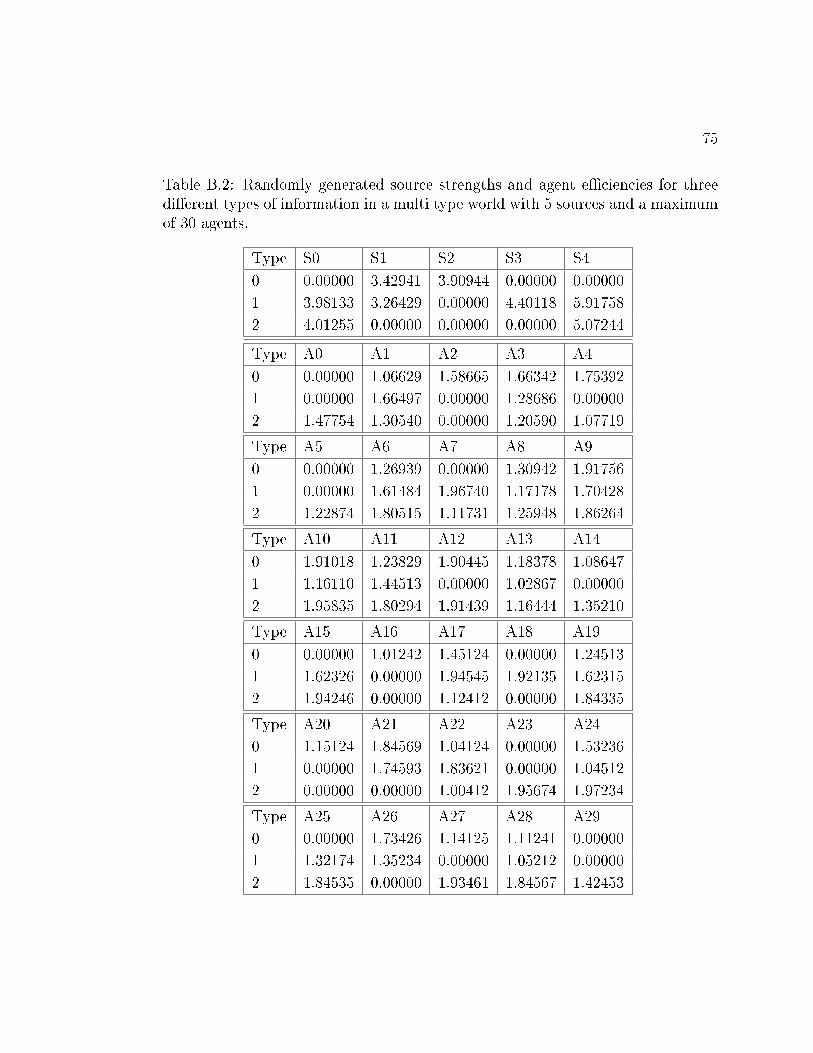
75
Table B.2: Randomly generated source strengths and agent e�ciencies for threedi�erent types of information in a multi type world with 5 sources and a maximumof 30 agents.
Type S0 S1 S2 S3 S40 0.00000 3.42941 3.90944 0.00000 0.000001 3.98133 3.26429 0.00000 4.40118 5.917582 4.01255 0.00000 0.00000 0.00000 5.07244
Type A0 A1 A2 A3 A40 0.00000 1.06629 1.58665 1.66342 1.753921 0.00000 1.66497 0.00000 1.28686 0.000002 1.47754 1.30540 0.00000 1.20590 1.07719
Type A5 A6 A7 A8 A90 0.00000 1.26939 0.00000 1.30942 1.917561 0.00000 1.61484 1.96740 1.17178 1.704282 1.22874 1.80515 1.11731 1.25948 1.86264
Type A10 A11 A12 A13 A140 1.91018 1.23829 1.90445 1.18378 1.086471 1.16110 1.44513 0.00000 1.02867 0.000002 1.95835 1.80294 1.91439 1.16444 1.35210
Type A15 A16 A17 A18 A190 0.00000 1.01242 1.45124 0.00000 1.245131 1.62326 0.00000 1.94545 1.92135 1.623152 1.94246 0.00000 1.12412 0.00000 1.84335
Type A20 A21 A22 A23 A240 1.15124 1.84569 1.04124 0.00000 1.532361 0.00000 1.74593 1.83621 0.00000 1.045122 0.00000 0.00000 1.00412 1.95674 1.97234
Type A25 A26 A27 A28 A290 0.00000 1.73426 1.14125 1.11241 0.000001 1.32174 1.35234 0.00000 1.05212 0.000002 1.84535 0.00000 1.93461 1.84567 1.42453