APPROVED:

Kamesh Namuduri, Major Professor Murali Varanasi, Committee Member Bill Buckles, Committee Member Shengli Fu, Chair of the Department of

Electrical Engineering Costas Tsatsoulis, Dean of the College of

Engineering Victor Prybutok, Dean of the Toulouse

Graduate School

FORMATION CONTROL OF MULTI-AGENT SYSTEMS

Srijita Mukherjee

Thesis Prepared for the Degree of

MASTER OF SCIENCE

UNIVERSITY OF NORTH TEXAS

August 2017

Mukherjee, Srijita. Formation Control of Multi-Agent Systems. Master of Science

(Electrical Engineering), August 2017, 43 pp., 1 table, 21 figures, 14 numbered references.

Formation control is a classical problem and has been a prime topic of interest among the

scientific community in the past few years. Although a vast amount of literature exists in this

field, there are still many open questions that require an in-depth understanding and a new

perspective. This thesis contributes towards exploring the wide dimensions of formation control

and implementing a formation control scheme for a group of multi-agent systems. These systems

are autonomous in nature and are represented by double integrated dynamics. It is assumed that

the agents are connected in an undirected graph and use a leader-follower architecture to reach

formation when the leading agent is given a velocity that is piecewise constant. A MATLAB code

is written for the implementation of formation and the consensus-based control laws are verified.

Understanding the effects on formation due to a fixed formation geometry is also observed and

reported. Also, a link that describes the functional similarity between desired formation

geometry and the Laplacian matrix has been observed. The use of Laplacian matrix in stability

analysis of the formation is of special interest.

ii

Copyright 2017

By

Srijita Mukherjee

iii

ACKNOWLEDGEMENTS

The fruits of success are always supported and nourished by its roots. I take this

opportunity to thank God for providing me with an extremely tranquil atmosphere at work and

cooperative people during the journey of my Masters at UNT. I express my immense gratitude to

my thesis advisor and mentor, Dr. Kamesh Namuduri. It was his knack of discussing innovative

ideas that motivated me to select the topic of my thesis. One of his greatest virtue was the belief

in giving me freedom to think.

I am grateful to Dr. Murali Varanasi and Dr. Bill Buckles who offered me their insights and

encouraged me to look beyond the thesis. I would like to thank all the faculty members and staff

from Department of Electrical Engineering, University of North Texas for being constant pillars of

support.

I find myself fortunate to have such loving and understanding parents who stood by me

through thick and thin during the last four semesters at UNT. My sincere thanks to them for their

continuous encouragement. Finally, I would like to thank Neha Kharate for being and working

with me prior to deadlines and all my other friends for being a source of great help.

iv

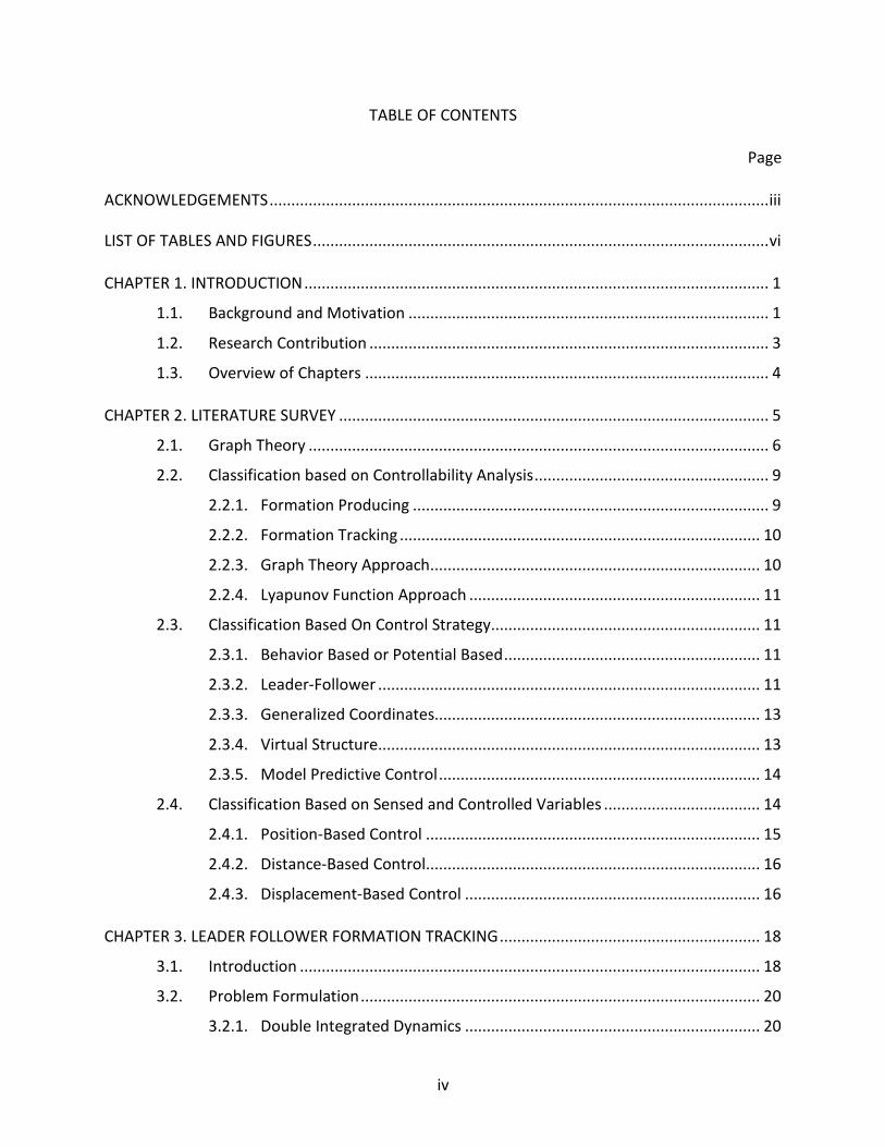
TABLE OF CONTENTS

Page

ACKNOWLEDGEMENTS ................................................................................................................... iii LIST OF TABLES AND FIGURES ......................................................................................................... vi CHAPTER 1. INTRODUCTION ........................................................................................................... 1

1.1. Background and Motivation ................................................................................... 1

1.2. Research Contribution ............................................................................................ 3

1.3. Overview of Chapters ............................................................................................. 4 CHAPTER 2. LITERATURE SURVEY ................................................................................................... 5

2.1. Graph Theory .......................................................................................................... 6

2.2. Classification based on Controllability Analysis ...................................................... 9

2.2.1. Formation Producing .................................................................................. 9

2.2.2. Formation Tracking ................................................................................... 10

2.2.3. Graph Theory Approach ............................................................................ 10

2.2.4. Lyapunov Function Approach ................................................................... 11

2.3. Classification Based On Control Strategy .............................................................. 11

2.3.1. Behavior Based or Potential Based ........................................................... 11

2.3.2. Leader-Follower ........................................................................................ 11

2.3.3. Generalized Coordinates........................................................................... 13

2.3.4. Virtual Structure ........................................................................................ 13

2.3.5. Model Predictive Control .......................................................................... 14

2.4. Classification Based on Sensed and Controlled Variables .................................... 14

2.4.1. Position-Based Control ............................................................................. 15

2.4.2. Distance-Based Control ............................................................................. 16

2.4.3. Displacement-Based Control .................................................................... 16 CHAPTER 3. LEADER FOLLOWER FORMATION TRACKING ............................................................ 18

3.1. Introduction .......................................................................................................... 18

3.2. Problem Formulation ............................................................................................ 20

3.2.1. Double Integrated Dynamics .................................................................... 20

v

3.2.2. Graph Topology ......................................................................................... 21

3.2.3. Formation Geometry ................................................................................ 23

3.3. Control Theory ...................................................................................................... 24

3.3.1. Centralized Control ................................................................................... 24

3.3.2. Distributed Control Approach ................................................................... 25

3.4. Consensus Control Law ......................................................................................... 27 CHAPTER 4. CONTROL DESIGN AND ALGORITHM ........................................................................ 29

4.1. Control Design ....................................................................................................... 29

4.1.1. Inputs ........................................................................................................ 29

4.1.2. Controller .................................................................................................. 30

4.1.3. Plant/System ............................................................................................. 31

4.2. Algorithm .............................................................................................................. 31 CHAPTER 5. RESULTS ..................................................................................................................... 33

5.1. Introduction .......................................................................................................... 33

5.2. Experiments .......................................................................................................... 33 CHAPTER 6. CONCLUSIONS AND FUTURE WORK ......................................................................... 42 REFERENCES .................................................................................................................................. 43

vi

LIST OF TABLES AND FIGURES

Page

Table 2.1: Differences between positon, displacement and distance-based formation control [3]. ................................................................................................................................................. 15

Figure 2.1: Example of Formation Control of UAVs with group reference [11] ............................. 6

Figure 2.2: Example of a simple graph. ........................................................................................... 8

Figure 2.3: 𝑙𝑙 − 𝜓𝜓 controller [6] ..................................................................................................... 12

Figure 2.4: 𝑙𝑙 − 𝑙𝑙 controller [6] ..................................................................................................... 13

Figure 2.5. Sensing capability vs interaction topology [3] ............................................................ 17

Figure 2.6: A sample architecture for formation [3] ..................................................................... 17

Figure 3.1: Vic formation .............................................................................................................. 18

Figure 3.2: Four Finger Formation [13] ......................................................................................... 19

Figure 3.3: Fly-past Formation [14] .............................................................................................. 19

Figure 3.4: MAS in undirected graph ............................................................................................ 21

Figure 3.5: Centralized control system ......................................................................................... 25

Figure 3.6: Distributed control System ......................................................................................... 26

Figure 3.7: A graphical comparison of centralized and distributed approach ............................. 26

Figure 4.1: Control design ............................................................................................................. 29

Figure 5.1: Agent trajectories for Vd = (1,-2) ................................................................................ 34

Figure 5.2: Agent trajectories in first quadrant ............................................................................ 35

Figure 5.3: Agent trajectories in second quadrant ....................................................................... 36

Figure 5.4: Agent trajectories for third quadrant ......................................................................... 37

vii

Figure 5.5: Agent Trajectories with sign reversal ......................................................................... 38

Figure 5.6: Agent trajectories with sign reversal in fourth quadrant ........................................... 39

Figure 5.7: Agent trajectories for higher desired velocity ............................................................ 40

1

CHAPTER 1

INTRODUCTION

1.1. Background and Motivation

Autonomous multi-agent systems (MAS) and their coordinated movement have been a

broad topic of research in the past few years. These systems are controlled by cooperative

control laws and are designed to act in a way that serves the group’s common purpose. Examples

of coordinated control (or collective behavior) can be found in the flocking of birds [5], consensus

problems, formation control of multiple agents and clustering as mentioned in [1]. The

abovementioned research problems are both independent and mutually overlapping. The prime

idea behind all these areas of study is “reaching a common agreement” or attaining “consensus”.

Consensus is a distributed estimation technique that is used for various cooperative

control capabilities applied to multi agent systems. When all the nodes in a sensor network or

agents in an MAS seem to arrive at a common value based on some algorithm, the network or

the MAS is said to reach consensus. A detailed review on application of consensus in MAS can be

found in [13]. Although it is an efficient technique, study of consensus on systems with multiple

physical parameters requires a different approach. This idea does not consider the group

formation, thus making it impractical for application in areas where agents need to form a pre-

defined group. In such applications, the moving of system of agents in formation is more

advantageous than a conventional system. A result of this re-calibration of an already existing

consensus problem is the “formation control.”

Formation control is an example of a cooperative control problem, where the goal is

stabilization of relative distances between agents and their neighbors based on some pre-defined

2

relative distance (or geometry). Unmanned air vehicles (UAV’s), civilian aircrafts and space

vehicles are thus controlled frequently. Also, with the influx of aircrafts and further increase in

the future, proper utilization of airspace is crucial. This would reduce drag on the aircrafts and

thus increase their fuel efficiency as stated in [2]. Formation flying is also practiced by military

pilots for aerial combat and is more advantageous than the conventional method. In fact, there

are a few established types of formation such as Vic formation, finger-four and fly-past.

Formation control is a classical problem that can be categorized in different levels. Every

aspect of a practical multi agent system has opened scope for deeper studies. Surveys on existing

research shows that classification has been done based on controllability analysis, control

strategies, sensed and controlled variables, group reference, and system dynamics. These are

detailed in the later chapters [3][4].

A single formation is the result of a control scheme applied on agents that are defined by

certain dynamics. The complexity of system dynamics of an agent increases manifold when an

MAS is considered. In the process, the system dynamics represents the behavior of the vehicles

that includes parameters like velocity, acceleration, position, etc. For instance, studies have been

done on agents with single integrator kinematics and double integrated dynamics [3]. Agents

modeled by these dynamics differ in their final states. The single integrator kinematic systems

have a constant final state, whereas the latter normally have dynamic final states. This varying

nature of final states propels the study of the network topology of the same.

The network topology is another deciding factor in the field of formation control.

Presence of an edge between nodes (modeled as agents) ensures required information

exchange, in the absence of which, reaching the desired formation can be seriously hampered. A

3

profound knowledge of Graph theory and applying its principles can be useful in the stability

analysis of a formation. The resultant Laplacian matrix and its eigenvalues also provide deep

insights about the network. In terms of sensed and controlled variables, position-based control

and distance-based control has been a topic of study among researchers [3]. In the position-

based approach, the agents actively control themselves and position themselves in formation

without the need of interaction. This requires a high sensing capability for the agents. On the

other hand, distance- based control allows the agents to interact among themselves and form

the desired pattern by controlling the inter-agent distance. Both the methods have their own

pros and cons in terms of high reliability on sensors and on the higher number of interactions.

This thesis intends to implement the formation of the system of agents using a distance-based

control law and study the mechanism of defining the desired formation geometry.

1.2. Research Contribution

The objective of this thesis is to obtain formation control of multi-agent systems using

control laws for a leader-follower architecture. It also contributes to the development of a

MATLAB based software for implementing the formation. A detailed review of the research done

in the field of formation control from recent years is also provided. This would aid the

identification of future work.

To study the applicability of the formation control laws with varying conditions, my

contribution towards this thesis was to:

• Develop software for implementation and verification of formation.

• Perform experiments with desired velocities in different quadrants.

4

• Observe the effects of a fixed formation geometry.

• Introduce solutions to correct the “lagging” of the leader.

• Understand the linkage between Laplacian matrix and set of neighbors in control laws.

• Observe the functional similarity in the usage of the relative position set and Laplacian matrix.

1.3. Overview of Chapters

Formation control is a classical problem that has been practiced since the advent of

aircraft and has been widely applied in various practical applications. This thesis presents the

tools and a detailed classification of the formation of agents.

Chapter 2 provides information about graph theory and matrices that are used in

modeling the topology of the multi-agent system. The concept of formation producing and

formation tracking is introduced. It also gives a detailed classification of formation control based

on controllability analysis, control strategies, sensed and controlled variables.

Chapter 3 delves deep inside the problem formulation and discusses about the distance-

based control problem. The agent dynamics, graph topology and formation geometry used for

the proposed problem is defined. Chapter 4 introduces the control flow of the discussed problem

and provides an algorithm for the developed system. Chapter 5 includes all the experiments done

and the results of agent trajectories subject to varying conditions. Finally, conclusion and future

works for this thesis are discussed in Chapter 6.

5

CHAPTER 2

LITERATURE SURVEY

One of the age-old procedures followed in engineering is applying principles of nature to

create innovative structures. The invention of the aero plane by the Wright Brothers is a living

example. Recently, the phenomenon of bird flocking, schooling of fishes and swarming of

bacteria has captured the interest of scientists. These can be viewed as a collective movement of

agents and can be applied to autonomous systems for different applications. Studies have been

done on defining the flocking behavior. The famous rules of flocking model proposed by Reynolds

[3] are i) cohesion, ii) separation and iii) alignment. The formation control problem has been

inspired from the flocking model. Generally, two broad categories have been defined in

formation control.

• Formation producing: This encompasses formation control design that enables the

agents to reach formation without any group reference.

• Formation tracking: This includes algorithm design that requires agents to reach

formation by following or by keeping track of a group reference.

Usually formation tracking is more challenging than formation producing because of the

group reference used. Also, the design algorithms for the former cannot be applied to the latter.

By definition, formation is attainment of a desired geometric order by agents. Resemblance of

the agents with nodes of a graph prompted researchers to use graph theory as a tool for analyzing

the formation problem.

6

Figure 2.1: Example of Formation Control of UAVs with group reference [11]

2.1. Graph Theory

The stability analysis of a formation often deals with multiple agents and therefore

multiple parameters. Graph theory plays an important role in defining the interconnection

between the agents and by expressing them in a matrix form. The topology of the graph can be

studied for stability analysis of the formation.

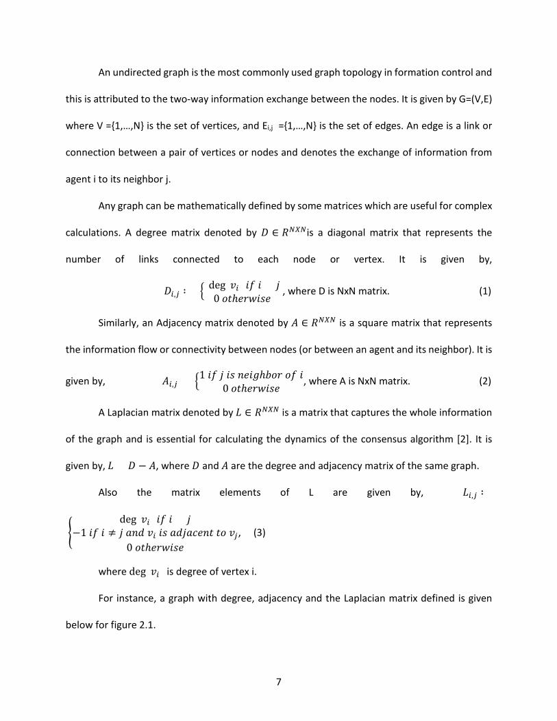
7

An undirected graph is the most commonly used graph topology in formation control and

this is attributed to the two-way information exchange between the nodes. It is given by G=(V,E)

where V ={1,…,N} is the set of vertices, and Ei,j ={1,…,N} is the set of edges. An edge is a link or

connection between a pair of vertices or nodes and denotes the exchange of information from

agent i to its neighbor j.

Any graph can be mathematically defined by some matrices which are useful for complex

calculations. A degree matrix denoted by 𝐷𝐷 ∈ 𝑅𝑅𝑁𝑁𝑁𝑁𝑁𝑁is a diagonal matrix that represents the

number of links connected to each node or vertex. It is given by,

𝐷𝐷𝑖𝑖,𝑗𝑗 ∶= �{deg(𝑣𝑣𝑖𝑖) 𝑖𝑖𝑖𝑖 𝑖𝑖 = 𝑗𝑗0 𝑜𝑜𝑜𝑜ℎ𝑒𝑒𝑒𝑒𝑒𝑒𝑖𝑖𝑒𝑒𝑒𝑒

, where D is NxN matrix. (1)

Similarly, an Adjacency matrix denoted by 𝐴𝐴 ∈ 𝑅𝑅𝑁𝑁𝑁𝑁𝑁𝑁 is a square matrix that represents

the information flow or connectivity between nodes (or between an agent and its neighbor). It is

given by, 𝐴𝐴𝑖𝑖,𝑗𝑗 = �1 𝑖𝑖𝑖𝑖 𝑗𝑗 𝑖𝑖𝑒𝑒 𝑛𝑛𝑒𝑒𝑖𝑖𝑛𝑛ℎ𝑏𝑏𝑜𝑜𝑒𝑒 𝑜𝑜𝑖𝑖 𝑖𝑖0 𝑜𝑜𝑜𝑜ℎ𝑒𝑒𝑒𝑒𝑒𝑒𝑖𝑖𝑒𝑒𝑒𝑒

, where A is NxN matrix. (2)

A Laplacian matrix denoted by 𝐿𝐿 ∈ 𝑅𝑅𝑁𝑁𝑁𝑁𝑁𝑁 is a matrix that captures the whole information

of the graph and is essential for calculating the dynamics of the consensus algorithm [2]. It is

given by, 𝐿𝐿 = 𝐷𝐷 − 𝐴𝐴, where 𝐷𝐷 and 𝐴𝐴 are the degree and adjacency matrix of the same graph.

Also the matrix elements of L are given by, 𝐿𝐿𝑖𝑖,𝑗𝑗 ∶=

�deg(𝑣𝑣𝑖𝑖) 𝑖𝑖𝑖𝑖 𝑖𝑖 = 𝑗𝑗

−1 𝑖𝑖𝑖𝑖 𝑖𝑖 ≠ 𝑗𝑗 𝑎𝑎𝑛𝑛𝑎𝑎 𝑣𝑣𝑖𝑖 𝑖𝑖𝑒𝑒 𝑎𝑎𝑎𝑎𝑗𝑗𝑎𝑎𝑎𝑎𝑒𝑒𝑛𝑛𝑜𝑜 𝑜𝑜𝑜𝑜 𝑣𝑣𝑗𝑗0 𝑜𝑜𝑜𝑜ℎ𝑒𝑒𝑒𝑒𝑒𝑒𝑖𝑖𝑒𝑒𝑒𝑒

, (3)

where deg(𝑣𝑣𝑖𝑖) is degree of vertex i.

For instance, a graph with degree, adjacency and the Laplacian matrix defined is given

below for figure 2.1.

8

Figure 2.2: Example of a simple graph.

The degree matrix is written as:

=

1000002000002000004000002

D ,

Adjacency matrix as:

=

0101010010000111110100110

A

Laplacian matrix, L=D-A as

−−−−

−−−−−−

−−

=

2101012010

0021111141

00112

L

9

Some properties of the Laplacian matrix are given below:

• It is a symmetric matrix

• The eigenvalues of L matrix provide a great deal of information about the network. For example, the second smallest eigenvalue (Fiedler value) represents the algebraic connectivity of a network.

• It is a singular matrix, i.e. the determinant of L matrix is zero.

• The diagonal elements are positive and the off-diagonal elements are negative.

2.2. Classification based on Controllability Analysis

Formation Producing

2.2.1.1. Graph Theory Approach

The principles of graph theory are frequently used for the stability and controllability analysis

of formation. The degree matrix, adjacency matrix and Laplacian matrix serve as tools for the

same as stated in [12]. The Eigen values of L matrix reveal much information about the stability

of the network.

Formation control of a fixed network topology displays the following two important

properties:

• Existence of at least one zero eigenvalue.

• At least one pair of eigenvalue on the imaginary axis in the system matrix of a linear closed loop system.

However, the complex analysis and working of switching network topology makes the

applicability of these properties very difficult and thus an open research problem [4]. Research

on formation stabilization where topology is represented by an undirected graph has been clearly

discussed in [6]. It states that spectral analysis of a graph plays a vital role in the control of multi

10

agent formation. It is also required that the graph is well connected for the usage of a linear

stabilizing feedback law. The smallest positive eigenvalue of the Laplacian matrix decides the time

taken to reach formation by the agents.

2.2.1.2. Lyapunov Function Approach

Lyapunov function approach is the most favored method used for stability analysis of

complex dynamical systems and control theory because the analysis of nonlinear systems is done

easily with the Lyapunov function than the graph theory approach (or matrix theory approach).

The types of formation producing that have been studied with this approach are the Inverse

agreement problem, the Leaderless flocking and stabilization, and the circular formation

problem. A brief review of these problems can be found in [4].

Formation Tracking

Graph Theory Approach

The formation tracking problem has also been studied by the graph theory or matrix

theory approach. The design of a control system that allows the agent to keep track of the

reference to reach a desired positon is interesting and has been discussed in detail in [4]. The

difference between the state of the agent and the reference is taken as an error. The goal of the

system would be to minimize the error and reduce it to zero. However, this method can only be

applied to the formation tracking system. This makes it easy for the formation tracking system to

be solved under a switching network topology.

11

Lyapunov Function Approach

The Lyapunov function is widely used for the stability analysis of systems. An example of

flocking with dynamic group reference has been discussed in [4] where the agents need to move

cohesively along the group reference. This study of a system with dynamic group reference is

more challenging than an unchanging group reference. This makes a leader follower problem

more complicated than leaderless flocking. The Lyapunov function has also been applied to

systems with variable structure-based control law to get better results.

2.3. Classification Based On Control Strategy

Behavior Based or Potential Based

Behavior based control strategy is used in MAS to fulfill navigational goals such as obstacle

avoidance, collision avoidance and maintaining the formation, as well. It is always combined with

the potential field approach. This control strategy enables individual agents or robotic vehicles

to concentrate on the inputs received by their sensors and act on it. Thus, all the agents in the

formation respond to information obtained from their surrounding areas and ensure full

coverage of formation. This kind of control action can be observed in air force fighter pilots who

restrict their visual and radar range to an area of terrain based on their current positions.

Applications of these methods in formation can be seen in search and rescue operations and

security patrol as mentioned in [7].

Leader-Follower

The formation of MAS using the Leader-follower control method has at least one leader

12

with the rest of the agents as followers. The control design is such that followers track the

position of the leader and the leader tracks its prescribed trajectory. This method is an example

of formation tracking with a reference. In [6], formation control with two types of feedback

controllers are discussed.

𝑙𝑙 − 𝜓𝜓 Controller: A desired length of 𝑙𝑙12𝑑𝑑 and a desired relative angle of 𝜓𝜓12𝑑𝑑 is maintained

between the leader and the follower, as shown below in Figure 2.2. Two-wheeled ground mobile

robots are examples where input/output feedback linearization can be used to design a

controller where 𝑙𝑙12𝑑𝑑 and 𝜓𝜓12𝑑𝑑 can achieve convergence.

Figure 2.3: 𝑙𝑙 − 𝜓𝜓 controller [6]

𝑙𝑙 − 𝑙𝑙 Controller: In the example mentioned in [6], the formation contains two leaders and

one follower. The follower robot is controlled to track and follow the leaders. The desired length

𝑙𝑙13𝑑𝑑 and 𝑙𝑙23𝑑𝑑 between the follower and leaders is maintained. The input/output feedback

linearization can be used in 𝑙𝑙 − 𝑙𝑙 controllers as well.

Mostly, nonlinear systems can be controlled by the feedback linearization method. The

conversion of a nonlinear system into a linear system is done by changing some of the variables

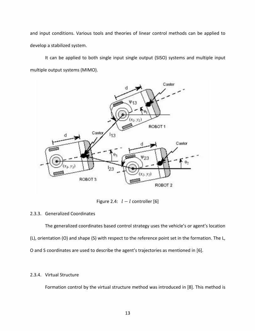
13

and input conditions. Various tools and theories of linear control methods can be applied to

develop a stabilized system.

It can be applied to both single input single output (SISO) systems and multiple input

multiple output systems (MIMO).

Figure 2.4: 𝑙𝑙 − 𝑙𝑙 controller [6]

Generalized Coordinates

The generalized coordinates based control strategy uses the vehicle’s or agent’s location

(L), orientation (O) and shape (S) with respect to the reference point set in the formation. The L,

O and S coordinates are used to describe the agent’s trajectories as mentioned in [6].

Virtual Structure

Formation control by the virtual structure method was introduced in [8]. This method is

14

used in applications where a fixed formation geometry is required. Spacecraft application in deep

space is an example. Also, in laser interferometry, the instruments are required to fixed

kilometers apart in space to get proper reading. The idea for this concept was derived from the

behavior of a rigid body. Particles in a rigid body are in a fixed geometry and any force or

disturbance made to one particle will propagate to all other particles comprising the body. Any

robotic system build using this concept was thought to be highly desirable as discussed in [8].

The controller of the virtual structure method follows three steps. Firstly, the desired

dynamics of the robotic structure to be built is defined. Secondly, each robot or agent is made to

follow the desired motion of the whole virtual structure. Thirdly, controllers to track each agent

are designed. Further details are discussed in [6].

Model Predictive Control

One of the recent coordinated control laws is the model predictive control (MPC). Agents

or robots are controlled locally by defining a local control law. Presence of inter vehicle

communication and the distributed nature of the control design takes care of the total formation.

This is desirable because a single agent cannot have access to a large-scale formation of agents.

This kind of control mechanism has been used in [9] on simple 1D vehicles.

2.4. Classification Based on Sensed and Controlled Variables

Any formation control scheme consists of variables that are sensed by agents and the

variables that are actively controlled. This is defined in terms of sensing capability and interaction

topology of the agents. The sensing capability of the formation is dependent on the types of

15

variables that are sensed. Also, the topology formed by the agents describes the type of

controlled variables needed. A detailed review is presented in [3].

There are ways in which the sensed and the controlled variables can be alternatively used

to decide the different types of controllers.

For instance, when the distances between the agents are controlled, then the agents

need to communicate with each other. Thus, the system would act like a rigid body. On the other

hand, when the positions of the agents are controlled directly, then the agents need not

communicate with each other. These kinds of variations are used to decide on the classifications.

Characterization Position-based Displacement-based Distance-based

Sensed Variables Position of agents Relative positions of neighbors

Relative positions of neighbors

Controlled Variables Position of agents Relative positions of neighbors Inter-agent distances

Coordinate Systems A global coordinate system

Orientation aligned local coordinate

systems

Local coordinate systems

Interaction Topology Usually not required Connectedness or

existence of a spanning tree

Rigidity or persistence

Table 2.1: Differences between positon, displacement and distance-based formation control [3].

Position-Based Control

A formation control scheme that has position-based control causes its agents to actively

control their positions with respect to the global coordinate system. The two components of this

method are sensing capability and interaction topology. Interaction among agents and feedback

16

taken from agents by a global coordinator are the two important steps in position-based

formation control.

Distance-Based Control

Distances between agents are actively controlled to reach formation. Each agent figures

out relative positions with respect to their neighbors based on the local coordinate system.

Sensing capability requires that agents know the local coordinate system. Since the desired

distances between agents (or desired formation) are fixed, the interaction topology should be

rigid. The agents use translational and rotational motions to reach formation.

Displacement-Based Control

Displacement between agents and their neighbors are actively controlled to reach

formation. The input is in the form of desired displacement-based on the global coordinate

system. The agents need to have knowledge of the orientation of the global coordinate system.

The choice of a control method is based on many different criteria that can be varied as

per application. Distance-based and displacement-based control using single and double

integrated dynamics have been given in detail in [3]. A review on the analysis comparing sensing

capability and interaction topology has also been mentioned.

17

Figure 2.5. Sensing capability vs interaction topology [3]

Figure 2.6: A sample architecture for formation [3]

Displacement -Based

Distance-Based

Position-Based

More advanced sensing

capability

More

18

CHAPTER 3

LEADER FOLLOWER FORMATION TRACKING

3.1. Introduction

Formation control of multi-agent systems has been a prime topic of interest over the

recent years. This kind of cooperative control mechanism has wide scale application. Formation

flying follows different patterns as shown below.

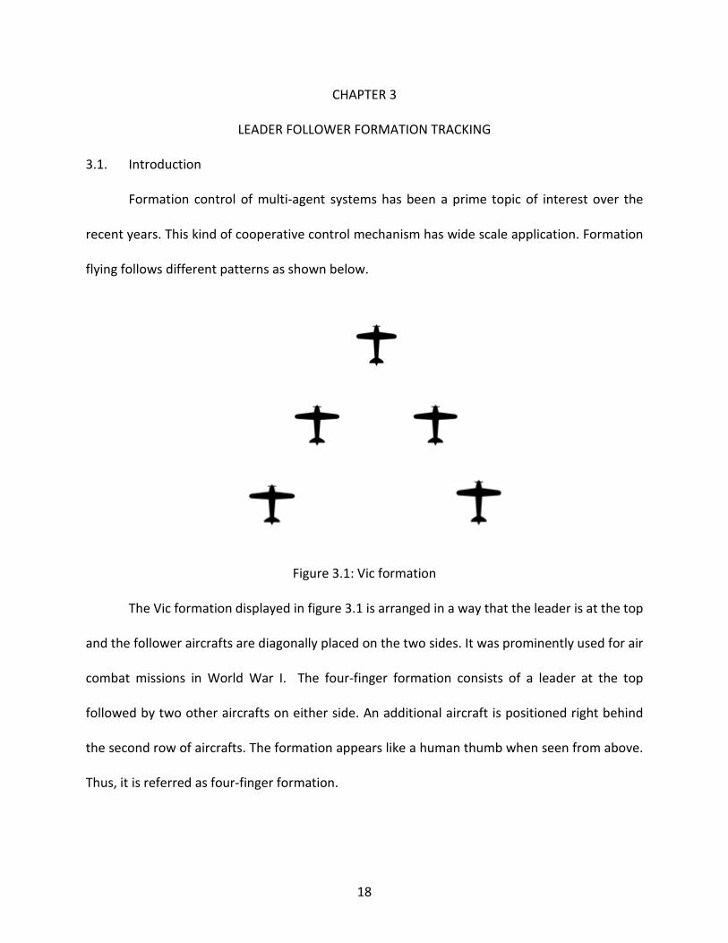
Figure 3.1: Vic formation

The Vic formation displayed in figure 3.1 is arranged in a way that the leader is at the top

and the follower aircrafts are diagonally placed on the two sides. It was prominently used for air

combat missions in World War I. The four-finger formation consists of a leader at the top

followed by two other aircrafts on either side. An additional aircraft is positioned right behind

the second row of aircrafts. The formation appears like a human thumb when seen from above.

Thus, it is referred as four-finger formation.

19

Figure 3.2: Four Finger Formation [13]

Figure 3.3: Fly-past Formation [14]

One of the most prominent and widely used patterns is the Vic or V formation. It is

basically a leader-follower architecture where at least one agent acts as leader and other agents

act as followers. This type of formation flying will be useful in the future when more aircraft

crowd the airspace. A single formation problem is built of various components. The whole control

design consists of agent dynamics, information topology, the pattern of formation and control

algorithms. This chapter begins with the definition of agent dynamics. It is followed by a

discussion about the information topology of the multi-agent system and modeling of matrices.

At the end, the consensus control laws are introduced.

20

3.2. Problem Formulation

The multi-agent systems considered for the formation problem follows a distance-based

control and is defined by double integrator dynamics. The agents in a distance-based formation

control sense the relative positions of their neighbors and actively control the inter-agent

distances. The interaction topology of the MAS is rigid or time-invariant. The objective of the

system is to track the leader’s position while maintaining a cohesive movement until the inter-

agent distances match the desired formation geometry. The working of the MAS is further

discussed in the following subsections.

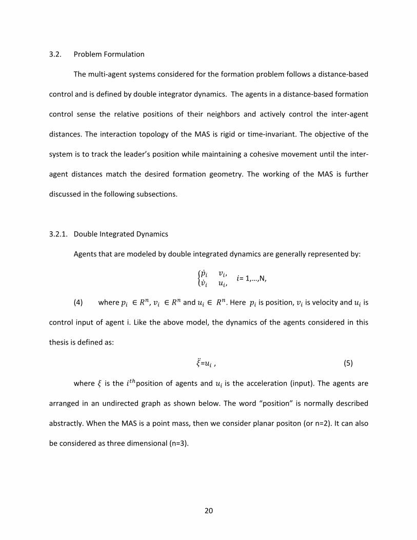
Double Integrated Dynamics

Agents that are modeled by double integrated dynamics are generally represented by:

��̇�𝑝𝑖𝑖 = 𝑣𝑣𝑖𝑖 ,�̇�𝑣𝑖𝑖 = 𝑢𝑢𝑖𝑖,

𝑖𝑖= 1,…,N,

(4) where 𝑝𝑝𝑖𝑖 ∈ 𝑅𝑅𝑛𝑛, 𝑣𝑣𝑖𝑖 ∈ 𝑅𝑅𝑛𝑛 and 𝑢𝑢𝑖𝑖 ∈ 𝑅𝑅𝑛𝑛. Here 𝑝𝑝𝑖𝑖 is position, 𝑣𝑣𝑖𝑖 is velocity and 𝑢𝑢𝑖𝑖 is

control input of agent i. Like the above model, the dynamics of the agents considered in this

thesis is defined as:

�̈�𝜉=𝑢𝑢𝑖𝑖 , (5)

where 𝜉𝜉 is the 𝑖𝑖𝑡𝑡ℎposition of agents and 𝑢𝑢𝑖𝑖 is the acceleration (input). The agents are

arranged in an undirected graph as shown below. The word “position” is normally described

abstractly. When the MAS is a point mass, then we consider planar positon (or n=2). It can also

be considered as three dimensional (n=3).

21

Graph Topology

The mathematical representation of an MAS-using graph topology has opened new doors

for analyzing the system. It is a simpler yet effective approach where information sent and

received from each vertex or node can be observed. The nodes in a graph can be imagined to

depict any type of system from the field of engineering, economics, human sciences, biology, etc.

This is the motivation behind using graph theory to form and analyze the MAS in this thesis.

Figure 3.4: MAS in undirected graph

The topology of the MAS offers much vital information about the system. The

representation of the multi-agent system in an undirected graph facilitates a two-directional

information exchange.

At least one link or edge exists between each pair of agents. Thus, all the agents can

communicate with one another and ensure that formation is achieved. The control strategy used

in this thesis is the leader-follower approach. One agent is designated as the leader and the other

agents as followers. Since it is also a formation tracking problem, where the agents track a group

reference to reach formation, a piecewise constant velocity command is given to the leader. This

constant velocity acts as the group reference.

22

Deciphering the graph topology into system matrices is useful for mathematical

calculations. It helps in understanding the connectivity of the nodes or agents and provides scope

for better analysis of the graphs. Various matrices have been used for such purposes. The

matrices for the undirected graph shown in Figure 8 can be written as:

Degree matrix,

=

1000002000002000003000002

D

The degree matrix is an n x n diagonal matrix where elements of the diagonal represent

the number of neighboring nodes of each vertex. Or, it gives the number of links attached to each

vertex. From the above degree matrix, it is deduced that agent 1 or the leader has two neighbors

(Agent 2 and Agent 3). Similarly, Agent 2 has 3 neighbors (Agent 1, 3 and 4). Similarly, such

information can be directly captured from the undirected graph shown in Figure 8.

Adjacency matrix,

=

0100010010000110110100110

A

The adjacency matrix is an n x n square matrix whose elements represent the neighboring

nodes connected to each vertex. As per definition, if a vertex is linked to a node, then

corresponding 𝐴𝐴𝑖𝑖𝑗𝑗 = 1. Here 𝑖𝑖 is the agent and 𝑗𝑗 is the neighbor of agent 𝑖𝑖. For an undirected

graph, the adjacency matrix is symmetric. The eigenvalues and eigenvectors are also used for

spectral analysis of the graph. Together, the degree and adjacency matrix capture the entire

23

information of a graph. The degree matrix shows the degree of each agent and the adjacency

matrix displays the connectivity of each agent.

Another important matrix in the graph theory is the Laplacian matrix. It is also addressed

differently as per application, namely, admittance matrix, Kirchhoff’s matrix or discrete Laplacian.

It is a representation of the entire graph. It can be written as L=D-A (i.e. difference of Degree and

Adjacency matrix).

−−−

−−−−−

−−

=

1100012010

002110113100112

L

The eigenvalues of L matrix are useful in many ways. L is also symmetric for an undirected

graph. Another important property of L states that it is positive-semidefinite. That is, L has an

eigenvalue of zero and 𝛿𝛿1 as its eigenvector.

Formation Geometry

One of the most important inputs in any formation control problem is the desired

Formation geometry. In the case of a distance-based control, the desired formation is fixed or

time-invariant irrespective of any translational or rotational motion. When the inter-agent

distances become equal to the distances specified by the desired geometry, then formation is

reached. There are many types of formation geometry such as triangle formation, line formation,

etc. Each of these types specifies the exact distance the agents should maintain to attain

formation.

24

The formation geometry in this problem is given by the relative position set, D. It is

defined as D = {𝑎𝑎𝑖𝑖𝑗𝑗 := ξ𝑖𝑖𝑖𝑖-ξ𝑗𝑗𝑖𝑖}, (6)

where ξ𝑖𝑖𝑖𝑖 is the desired position of the 𝑖𝑖𝑡𝑡ℎ agent and ξ𝑗𝑗𝑖𝑖 is the desired position of 𝑗𝑗𝑡𝑡ℎ.

Also, agent 𝑖𝑖 and 𝑗𝑗 are neighbors of each other.

3.3. Control Theory

Over the last few decades, control theory has attained immense popularity resulting in a

wide range of applications. It started with the first flight of the Wright Brothers. Since then, it has

been used in electronic devices, automation systems, missile navigation systems, fire control

systems, etc. A rising use was seen during World War II. The field of control theory has seen a lot

of developments so far. Some of them are PID controllers, fuzzy logic controllers, adaptive

controllers, nonlinear controllers, etc. A detailed review can be found in [4].

Control of vehicles has gained increased interest from researchers and it was deemed that

replacing a single complicated vehicle with multiple simpler vehicles was beneficial. Because of

this conclusion, two broad subdivisions came into being. Today modern control theory has two

approaches for controlling multiple vehicles. They centralized control and decentralized control

(or distributed approach).

Centralized Control

In a centralized control system, the controller exerts direct control over the all the middle

and lower level systems using a power hierarchy. It is a complicated process and is used in many

practical applications.

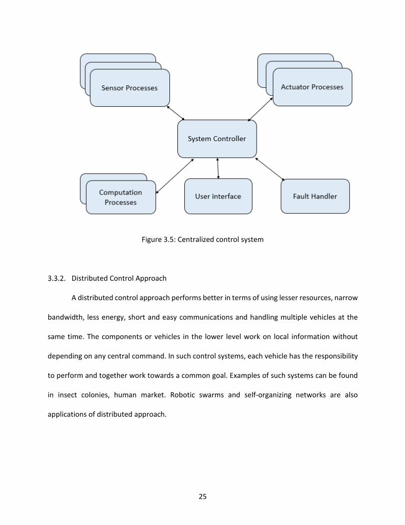
25

Figure 3.5: Centralized control system

Distributed Control Approach

A distributed control approach performs better in terms of using lesser resources, narrow

bandwidth, less energy, short and easy communications and handling multiple vehicles at the

same time. The components or vehicles in the lower level work on local information without

depending on any central command. In such control systems, each vehicle has the responsibility

to perform and together work towards a common goal. Examples of such systems can be found

in insect colonies, human market. Robotic swarms and self-organizing networks are also

applications of distributed approach.

26

Figure 3.6: Distributed control System

Figure 3.7: A graphical comparison of centralized and distributed approach

27

3.4. Consensus Control Law

Consensus is a cooperative control method that is based on distributed approach.

Application of consensus laws to any multiple agent system results in fixed and agreed final state

of the system. When consensus is applied to an MAS with single integrator kinematics, a constant

final value is obtained. In the case of application to an MAS with double integrator dynamics (as

found in this thesis) a dynamic final value is obtained.

In the present problem, consensus control laws are applied to MAS where the group

formation is taken into consideration. This results in the problem to be termed as Formation

Control using Consensus control laws.

The graph topology of the MAS presented in Figure 3.4 is considered for the problem.

Each agent is denoted by 𝑖𝑖 and 𝑁𝑁𝑖𝑖 is the set of neighbors of agent 𝑖𝑖. There are five agents in the

system. The set of neighbors is given by:𝑁𝑁1 = {2,3}, 𝑁𝑁2 = {1,3,4}, 𝑁𝑁3 = {1,2}, 𝑁𝑁4 = {2,5} and

𝑁𝑁5 = {4}.

The Agent 1 is assigned as leader and rest of the agents as followers. The leader is given

a velocity command that is piecewise constant. That is the velocity is locally constant in

connected regions separated by some low dimensional boundaries as detailed in [10].

ξ̇1𝑖𝑖 = 𝑣𝑣𝑖𝑖 (7)

The goal of the MAS is to track the leader’s position, maintain and reach the desired

formation starting from any initial position or velocity.

The consensus control law for follower is given by:

𝑢𝑢𝑖𝑖 = −[𝑘𝑘𝑝𝑝𝑦𝑦𝑝𝑝𝑖𝑖 + 𝑘𝑘𝑒𝑒𝑦𝑦𝑟𝑟𝑖𝑖] + 𝑘𝑘𝑝𝑝∑ 𝑎𝑎1𝑗𝑗𝑗𝑗∈𝑁𝑁1 , (8)

28

where, i = 2,….,N, 𝑦𝑦𝑝𝑝𝑖𝑖 = ∑ (ξ i − ξ j)𝑗𝑗∈𝑁𝑁1 (9)

and 𝑦𝑦𝑟𝑟𝑖𝑖 = � ��̇�𝜉𝑖𝑖 − �̇�𝜉𝑗𝑗�𝑗𝑗∈𝑁𝑁1 (10)

Here �̇�𝜉𝑖𝑖 represents the velocity of the follower agent and �̇�𝜉𝑗𝑗 is the velocity of its

neighboring agents. Therefore, relative velocity and relative positions between the agents are

used to calculate the 𝑢𝑢𝑖𝑖 (i.e. input).

Similarly, the control law for the leader is given by:

u1 = utr - � 𝑘𝑘𝑝𝑝(ξ 1 − ξ j) + 𝑘𝑘𝑒𝑒��̇�𝜉1 − �̇�𝜉𝑗𝑗� − 𝑘𝑘𝑝𝑝𝑎𝑎1𝑗𝑗𝑗𝑗∈𝑁𝑁1 , (11)

where utr = −[𝑘𝑘𝑝𝑝(ξ1 − ξ1D) + 𝑘𝑘𝑒𝑒(�̇�𝜉1 − 𝑣𝑣𝑖𝑖)] (12)

is the tracking component of the leader.

Here, 𝑣𝑣𝑖𝑖 is the desired velocity. Agents i and j are neighbors to each other. ξi is the initial

position of the ith agents and ξj is the initial position of j neighboring agents.

29

CHAPTER 4

CONTROL DESIGN AND ALGORITHM

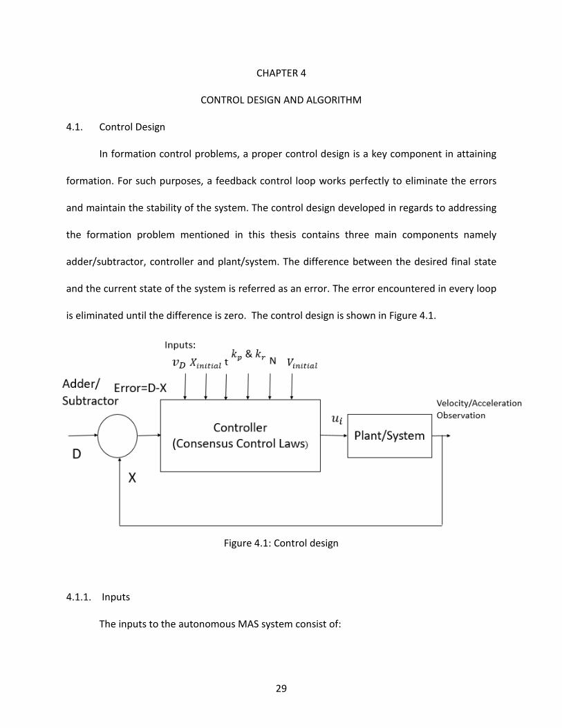
4.1. Control Design

In formation control problems, a proper control design is a key component in attaining

formation. For such purposes, a feedback control loop works perfectly to eliminate the errors

and maintain the stability of the system. The control design developed in regards to addressing

the formation problem mentioned in this thesis contains three main components namely

adder/subtractor, controller and plant/system. The difference between the desired final state

and the current state of the system is referred as an error. The error encountered in every loop

is eliminated until the difference is zero. The control design is shown in Figure 4.1.

Figure 4.1: Control design

Inputs

The inputs to the autonomous MAS system consist of:

30

• The desired formation geometry (D) as given by Eq (6): D is the summation of

desired relative distances between the agents and their neighbors. Varying the desired relative

distances yields in different formation shapes. Examples of other formation include Line

formation, triangular formation, finger four formation and V formation.

• Desired velocity (𝑣𝑣𝑖𝑖): The desired velocity is given is terms of X and Y coordinates

and can refer to four different quadrants of the graph. This helps in deciding the direction of

the agent trajectories. For example, 𝑣𝑣𝑖𝑖= (1,2).

• Time constant (t): The time constant is used to determine the time required to reach

formation. It is multiplied with the iteration number to identify the location of an agent in its

trajectory.

• Initial position: The system is designed such that formation can be achieved starting

from any initial position.

• Initial velocity: The agents or vehicles can be at any initial velocity to reach

formation. Different experimental cases are shown in Chapter 5.

• Scalar constants (𝑘𝑘𝑝𝑝 and 𝑘𝑘𝑟𝑟): These constants basically refer to the forces acting on

the aircraft or UAV.

• Number of vehicles: The number of agents or vehicles assumed for this problem is

five. However, formation for multiple agents can also be obtained using the same procedure.

Controller

The Consensus control laws explained by eq (8) and (11) in Chapter 3 form the controller

for the formation problem. The control law for the leader given by eq (11) is a combination of

31

tracking component 𝑢𝑢𝑡𝑡𝑟𝑟 and a summation component. The desired position of the leader ξ1𝑖𝑖 and

the desired velocity 𝑣𝑣𝑖𝑖 are inputs to the tracking component. The desired velocity act as the

group reference in the context of formation tracking.

The follower’s control law is also a sum of some important physical parameters. It consists

of aggregated relative position (𝑦𝑦𝑝𝑝𝑖𝑖) and velocity (𝑦𝑦𝑟𝑟𝑖𝑖) and formation geometry.

The controller performs calculations on both the leader’s and follower’s control equations

simultaneously and provides the acceleration, 𝑢𝑢𝑖𝑖 as the output. 𝑢𝑢𝑖𝑖 acts as the control input for

the Plant/System.

Plant/System

The output of the controller acts as the control input to the plant/system. In real time

applications, the navigation unit of a vehicle or robot can be referred as the plant/system. Such

systems enable in course correction of the vehicle. GPS (Global Positioning System) is also a

navigation unit that is broadly used. In a similar fashion, the control input is observed and the

decision to continue the feedback loop is taken based on the new position values calculated.

4.2. Algorithm

The formation control problem implemented and studied in this thesis is written in the

MATLAB software. The procedure followed is clearly represented by an algorithm given below.

STEP 1: START

STEP 2: Get the inputs

𝑘𝑘𝑝𝑝 and 𝑘𝑘𝑟𝑟

32

t,

N (Number of agents),

Initial positions of agents,

Initial velocities of agents,

Desired velocity (𝑣𝑣𝑖𝑖)

Desired formation of agents (D).

STEP 3: Initialize For loop

STEP 4: Calculate 𝑦𝑦𝑝𝑝𝑖𝑖 and 𝑦𝑦𝑟𝑟𝑖𝑖

STEP 5: Calculate 𝑢𝑢1 for leader and 𝑢𝑢𝑖𝑖 for followers

STEP 6: Obtain new position of agents

STEP 7: Check for error (E = D - X)

STEP 8: If E ≠ 0, Repeat For Loop

STEP 9: Otherwise, END For Loop

STEP 10: Plot the X and Y positions.

STEP 11: END

The parameter that decides the subsequent positions of all the agents is ξ1𝑖𝑖. It is the

desired position of agent 1 (the leader). This is due to fact that a piecewise constant velocity

command is given to the leader as given by eq (7). Thus, it can be concluded that ξ1𝑖𝑖 is time

varying. The cohesive movement of the agents is observed because ξ1𝑖𝑖 keeps changing in every

iteration and thus the parameters of follower agents also keep updating. In a way, desired

velocity 𝑣𝑣𝑖𝑖 (which is fixed or time-invariant) is the group reference for the formation problem

and ξ1𝑖𝑖 is the only variable that decides the values of the agent parameters in every iteration.

33

CHAPTER 5

RESULTS

5.1. Introduction

This chapter discusses the experiment and results obtained for different cases and inputs

that affect formation of a multi-agent system. The formation of five agents has been

implemented using MATLAB. There are some parameters that affect the system such as time

constant, desired velocity and desired geometry. Different aspects of the experiment conducted

have been displayed in the following few results.

5.2. Experiments

The first experiment is done for a system of five agents with initial position as:

% initial X and Y position

X(1,:)=[-5 3];

X(2,:)=[6.5 -3];

X(3,:)=[-7 7.5];

X(4,:)=[-3 7];

X(5,:)=[6.2 3.5];

The scalar constants are: Kp=10, Kr=5

Time constant: 0.008 sec

Number of iterations required: 1500

Desired velocity: 𝑣𝑣𝑖𝑖 = (1,-2)

Desired Formation Geometry for V formation:

34

D(1,:)=[1.3 -2.8]; D(2,:)=[-1.7 -0.3]; D(3,:)=[1.9 2.6]; D(4,:)=[-4.7 -1.5]; D(5,:)=[3.2 2]; The same formation geometry is used for all the following results.

1. The system of agents showed in Figure 5.1 attains formation by t = 12 seconds.

Locations of agents in intermediate position are also shown. The formation is almost

obtained by t = 8 seconds. At 12 seconds, the error calculated between current

positions and desired position reduces to zero.

Figure 5.1: Agent trajectories for Vd = (1,-2)

35

2. The formation shown in Figure 5.2 is based on the same input conditions except for

the desired velocity. In this case 𝑣𝑣𝑖𝑖 = (1, 2), i.e. velocity is in first quadrant. Thus, the

agent trajectories also move in the first quadrant. However, the desired formation

geometry remains the same as in Figure 5.1. This is because D is fixed (or time

invariant).

Figure 5.2: Agent trajectories in first quadrant

3. The result displayed in Figure 5.3 is also based on similar input conditions. The desired

velocity is given in second quadrant, i.e. 𝑣𝑣𝑖𝑖= (-1, 2).

36

Figure 5.3: Agent trajectories in second quadrant

4. The agent trajectories displayed in Figure 5.4 has the desired velocity in the third

quadrant, i.e. 𝑣𝑣𝑖𝑖= (-1,-2). In all these cases, the D remains fixed and the leader

appears to be lagging from the followers.

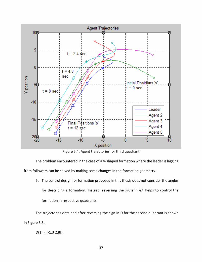
37

Figure 5.4: Agent trajectories for third quadrant

The problem encountered in the case of a V-shaped formation where the leader is lagging

from followers can be solved by making some changes in the formation geometry.

5. The control design for formation proposed in this thesis does not consider the angles

for describing a formation. Instead, reversing the signs in D helps to control the

formation in respective quadrants.

The trajectories obtained after reversing the sign in D for the second quadrant is shown

in Figure 5.5.

D(1,:)=[-1.3 2.8];

38

D(2,:)=[1.7 0.3]; D(3,:)=[-1.9 -2.6]; D(4,:)=[4.7 1.5]; D(5,:)=[-3.2 -2];

Figure 5.5: Agent Trajectories with sign reversal

6. Using the reversed desired formation in the fourth quadrant, the trajectory for the

leader appears to be lagging from other follower agents in Figure 5.6.

39

Figure 5.6: Agent trajectories with sign reversal in fourth quadrant

7. Agent trajectories are obtained for a higher velocity, 𝑣𝑣𝑖𝑖 = (10,6) and for t=0.007 sec.

Also the initial velocities of the five agents are:

V(1,:)=[10 20];

V(2,:)=[2 1];

V(3,:)=[5 4];

V(4,:)=[3 -5];

V(5,:)=[7 6];

40

The time taken to reach formation in this case is 6.65 sec. So, it is inferred that

formation is achieved faster when the velocity of the leader is increased.

Figure 5.7: Agent trajectories for higher desired velocity

8. Inferences from the control laws show that the set of neighbors, 𝑁𝑁𝑖𝑖 match with the

diagonal elements of the L matrix. They are given by: 𝑁𝑁1 = {2,3}, 𝑁𝑁2 = {1,3,4}, 𝑁𝑁3 =

{1,2}, 𝑁𝑁4 = {2,5} and 𝑁𝑁5 = {4}. The diagonal elements of L matrix represent the

number of neighbors of an agent 𝑖𝑖 and a ‘1’ or ‘0’ in off-diagonal elements indicate

links to the neighbors. This is due to the definition of L matrix, i.e. L=D-A. Thus, the

information from L matrix can be related to that used in the control laws.

9. An interesting observation is also made that links the desired formation geometry D and

the Laplacian matrix. This can aid in better understanding of the relative position of

41

agents. The formation geometry can be written as a system of five linear equations with

five unknowns.

2𝑎𝑎1 − 𝑎𝑎2 − 𝑎𝑎3 = (1.3,−2.8) (13)

3𝑎𝑎2 − 𝑎𝑎1 − 𝑎𝑎3 − 𝑎𝑎4 = (−1.7,−0.3) (14)

2𝑎𝑎3 − 𝑎𝑎1 − 𝑎𝑎2 = (1.9, 2.6) (15)

2𝑎𝑎4 − 𝑎𝑎2 − 𝑎𝑎5 = (−4.7,−1.5) (16)

𝑎𝑎5 − 𝑎𝑎4 = (3.2, 2) (17)

Here 𝑎𝑎1, 𝑎𝑎2, 𝑎𝑎3, 𝑎𝑎4 and 𝑎𝑎5 represent ξ1𝑖𝑖, ξ2𝑖𝑖, ξ3𝑖𝑖, ξ4𝑖𝑖 and ξ5𝑖𝑖 respectively.

Laplacian matrix can also be used to derive the system of equations (13 - 17) directly.

Therefore, usage of both the relative position set D and Laplacian matrix have a striking

similarity.

42

CHAPTER 6

CONCLUSIONS AND FUTURE WORK

The formation control of autonomous multi-agent system has been presented. Also,

MATLAB based simulation technique has been developed to experimentally verify the consensus

control laws. An undirected graph was used as the information topology of the multiple agents

and a leader-follower approach was chosen. The piecewise constant velocity command given to

the leader acts as the group reference. Formation for velocities given in different quadrants is

obtained. An observed problem with the present control design is the fixed nature of desired

formation geometry. It can be solved by reversing the signs in given formation geometry. A

functional similarity between the relative position set D and Laplacian matrix has also been

observed and reported. Also, the information found in L matrix has been found to be related to

control laws. Thus, Laplacian matrix can be used to summarize a system very well.

Works done on coordinated control of vehicles or robots and the various landmarks

achieved in the past few years have been researched. There is a lot of scope in this field and other

techniques for formation control can be explored. Optimization of network topology is a topic

that can be studied to find a perfect information topology. Stability analysis of the formation

obtained is another future work that would enable to test a broad range of input conditions.

Stabilization of formation using Lyapunov functions are briefly mentioned in [14]. Developing a

collision avoidance system using the current consensus control laws can also be another possible

future work.

43

REFERENCES

[1] Bai, He, Murat Arcak, and John Wen. Cooperative control design: a systematic, passivity-based approach. Springer Science & Business Media, 2011, pp.1-2

[2] Joshi, Suresh, and Oscar R. Gonzalez. "Consensus-Based Formation Control of a Class of Multi-Agent Systems." (2014)

[3] Oh, Kwang-Kyo, Myoung-Chul Park, and Hyo-Sung Ahn. "A survey of multi-agent formation control." Automatica 53 (2015): 424-440

[4] Cao, Yongcan, et al. "An overview of recent progress in the study of distributed multi-agent coordination." IEEE Transactions on Industrial informatics 9.1 (2013): 427-438.

[5] Pettit, Benjamin, et al. "Speed determines leadership and leadership determines learning during pigeon flocking." Current Biology 25.23 (2015): 3132-3137.

[6] Chen, Yang Quan, and Zhongmin Wang. "Formation control: a review and a new consideration." Intelligent Robots and Systems, 2005.(IROS 2005). 2005 IEEE/RSJ International Conference on. IEEE, 2005.

[7] Balch, Tucker, and Ronald C. Arkin. "Behavior-based formation control for multirobot teams." IEEE transactions on robotics and automation 14.6 (1998): 926-939.

[8] Tan, Kar-Han, and M. Anthony Lewis. "Virtual structures for high-precision cooperative mobile robotic control." Intelligent Robots and Systems' 96, IROS 96, Proceedings of the 1996 IEEE/RSJ International Conference on. Vol. 1. IEEE, 1996.

[9] Yan, Jun, and Robert R. Bitmead. "Coordinated control and information architecture." Decision and control, 2003. proceedings. 42nd ieee conference on. Vol. 4. IEEE, 2003.

[10] Lafferriere, Gerardo, et al. "Decentralized control of vehicle formations." Systems & control letters 54.9 (2005): 899-910.

[11] Chao, Zhou, et al. "UAV formation flight based on nonlinear model predictive control." Mathematical Problems in Engineering 2012 (2012).

[12] Olfati-Saber, Reza, J. Alex Fax, and Richard M. Murray. "Consensus and cooperation in networked multi-agent systems." Proceedings of the IEEE 95.1 (2007): 215-233.

[13] Chen, Yao, et al. "Multi-agent systems with dynamical topologies: Consensus and applications." IEEE circuits and systems magazine 13.3 (2013): 21-34.

[14] Ren, Wei, Randal W. Beard, and Ella M. Atkins. "Information consensus in multivehicle cooperative control." IEEE Control Systems 27.2 (2007): 71-82.