Aerodynamics of Track Cycling of Track Cycling ... model showed that the drag area and air density...
298
Aerodynamics of Track Cycling By Lindsey Underwood A thesis presented for the Degree of Doctor of Philosophy at The University of Canterbury Department of Mechanical Engineering Christchurch, New Zealand June 2012
Transcript of Aerodynamics of Track Cycling of Track Cycling ... model showed that the drag area and air density...

Aerodynamics of Track Cycling
By Lindsey Underwood
A thesis presented for the Degree of
Doctor of Philosophy
at
The University of Canterbury
Department of Mechanical Engineering
Christchurch, New Zealand
June 2012

i
Abstract
The aim of this thesis was to identify ways in which the velocity of a track cyclist could be increased, primarilythrough the reduction of aerodynamic drag, and to determine which factors had the most significant impacton athlete performance. An appropriate test method was set up in the wind tunnel at the University ofCanterbury to measure the aerodynamic drag of di!erent cycling positions and equipment, including helmets,skinsuits, frames and wheels, in order to measure the impact of specific changes on athlete performance.Rather than comparing standard cycling positions, such as the Obree, dropped, upright and aero positions,a number of individual and multiple changes were made to the height, width and length of the handlebars,seat height, head and helmet position, and hand position to provide a rank of importance in terms of whichchanges had the greatest impact (gain or loss) on the aerodynamic drag.
A mathematical model of the Individual Pursuit (IP) event was also created to calculate the velocity profileand finishing time for athletes competing under di!erent race conditions. The model was created in MicrosoftExcel and used first principles to analyse the forces acting on a cyclist, which lead to the development ofequations for power supply and demand. The model included the e!ects of leaning in the bends, and usedSRM power data to determine the actual position of the rider on the track. The mathematical model wasvalidated using SRM data for eleven, elite track cyclists, and was found to be accurate to 0.31s (0.16%).An analysis of changes made to the bike, athlete, and environmental conditions using the mathematicalmodel showed that the drag area and air density had the greatest impact on the finishing time. As the airdensity is fixed for all athletes competing in the same race, these results suggest that athletes should focuson minimising their drag area in order to maximise performance. The model was then used to predict thefinishing times for di!erent pacing strategies by generating di!erent power profiles for a given athlete with afixed stock of energy (the work done remained the same for all generated power profiles) in order to identifythe optimal pacing strategy for the IP. A comparison of the predicted finishing times for the di!erent pacingstrategies showed that an all-out and even or all-out and variable strategy with an initial acceleration phaseof 12s resulted in the fastest finishing time for a male, IP athlete with a fixed stock of energy whose e"ciencyis not a function of power output or speed. The length of time spent in the initial acceleration phase wasfound to have a significant impact on the results, although all strategies simulated with an initial accelerationphase resulted in a faster finishing time than all other strategies simulated.
Results from the wind tunnel tests also showed that, in general, changes made to the position of the cyclisthad the greatest impact on the aerodynamic drag compared to changes made to the equipment. Multiplechanges in position had a greater impact on drag than individual changes in position, but the changes werenot additive; the total gain or loss in drag for multiple changes in position was not the sum of individualgains or losses in drag. Actual gains and losses also varied significantly between athletes, primarily due todi!erences in body size and shape, riding experience, and reference position from which changes were madefrom. However, certain changes in position or equipment had a significant impact (>±1%) on the drag of allathletes tested compared to the reference position. For example, by wearing a shoe cover all athletes showeda reduction in drag of >1% regardless of shoe, cleat or pedal worn. Changes in position that resulted in areduction of the frontal area, such as lowering the handlebars and head, were the most successful at reducingthe aerodynamic drag, and a change in skinsuit was found to have the greatest impact on drag out of allequipment changes, primarily due to the choice of material and seam placement. The mathematical modelwas used to quantify the impact of changes in position and equipment made in the wind tunnel on the overallfinishing time for a given athlete competing in an IP event. Time savings of up to 8 seconds were seen for

ii
multiple changes in position, and up to 5 seconds for changes to the equipment.
Overall this thesis highlights the significance of aerodynamics on athlete performance in track cycling, sug-gesting that it is worthwhile spending time and money on research and technology to find new ways to reducethe aerodynamic drag and maximise the speed of cyclists. Although this thesis primarily concentrates on theIndividual Pursuit event in track cycling, the same principles can be applied to other cycling disciplines, aswell as to other sports.

iii
Acknowledgements
I would like to thank Dr Mark Jermy for giving me the opportunity to carry out this research and providingme with support and encouragement throughout my time at the University of Canterbury. My thanks alsoextend to the technicians Graeme Harris and Eric Cox for assisting me with all the testing and procedurescarried out in the wind tunnel, and also to my co-supervisor Stephanie Gutschmidt for her general support.
Thanh, Laura and Lisa, I could not have got through the past few years without having such great o"cemates. Those morning chats are invaluable, and you have provided great friendship and support that I hopewill continue when we go our separate ways.
Thanks to BikeNZ, SPARC, the REC centre, and all the athletes and coaches who provided data for mythesis, gave me the opportunity to get involved in the High Performance Programme, and helped me attendconferences and competitions to develop my knowledge in sports engineering and track cycling. I must alsothank Stuart McIntyre for his outstanding knowledge on apparel design, and for his enthusiam throughoutthe skinsuit project - you have been a pleasure to work with, and I hope that we can work together again inthe future.
I would like to show my appreciation to all the international students who have worked with me in the windtunnel and on projects related to my thesis. Particular thanks must go to Jana, Julien, and Amaury for theirhard work and also the entertainment they provided.
I am grateful to my flatmates, my friends, and of course my boyfriend, who have all made my time inNew Zealand so enjoyable. You have provided me with a home away from home, and a friendship andcompanionship that I am sure will last a lifetime. Finally my thanks must go to my parents and my brother.Without your continuous love and support, even when I am the other side of the world, I would not be whereI am today.

iv
List of Publications
1. L. Underwood and M.C. Jermy, Mathematical model of track cycling: the individual pursuit, TheEngineering of Sport 8, 2 (2): 3217–3222, 2010.
2. L. Underwood and M.C. Jermy, Optimal hand position for individual pursuit athletes, The Engineeringof Sport 8, 2 (2): 2425–2429, 2010.
3. L. Underwood and M.C. Jermy, Fabric testing for cycling skinsuits, 5th Asia-Pacific Congress on SportsTechnology (APCST), 13: 350-356, 2011.
4. L. Underwood, J. Schumacher, J. Burette-Pommay and M. Jermy, Aerodynamic drag and biomechanicalpower of a track cyclist as a function of shoulder and torso angles, Sports Engineering, 14 (2-4): 147-154,2011.
5. L. Underwood and M.C. Jermy, Determining the optimal pacing strategy for the track cycling individualpursuit event with a fixed energy mathematical model, Submitted to Sports Engineering - in review,May 2012.
6. L. Underwood and M.C. Jermy, Optimal handlebar position for individual pursuit athletes, Submittedto Sports Engineering - in review, May 2012.

Contents
1 Introduction 1
1.1 Motivation for research . . . . . . . . . . . . . . . . . . . . . . . . . . . . . . . . . . . . . . . . 1
1.2 Aims and Objectives . . . . . . . . . . . . . . . . . . . . . . . . . . . . . . . . . . . . . . . . . 1
1.3 Thesis Structure . . . . . . . . . . . . . . . . . . . . . . . . . . . . . . . . . . . . . . . . . . . 2
2 Background 3
2.1 Factors A!ecting Power Supply . . . . . . . . . . . . . . . . . . . . . . . . . . . . . . . . . . . 7
2.2 Factors A!ecting Power Demand . . . . . . . . . . . . . . . . . . . . . . . . . . . . . . . . . . 11
3 Literature Review 13
3.1 Literature Review: Mathematical Model . . . . . . . . . . . . . . . . . . . . . . . . . . . . . . 13
3.1.1 Types of Models . . . . . . . . . . . . . . . . . . . . . . . . . . . . . . . . . . . . . . . 14
3.1.1.1 Supply, Demand, and Supply-Demand Models . . . . . . . . . . . . . . . . . 14
3.1.1.2 Goodness of Fit and First Principle Models . . . . . . . . . . . . . . . . . . . 15
3.1.2 Existing Models for Cycling . . . . . . . . . . . . . . . . . . . . . . . . . . . . . . . . . 15
3.1.2.1 Aerodynamic Drag . . . . . . . . . . . . . . . . . . . . . . . . . . . . . . . . . 16
3.1.2.2 Rolling Resistance . . . . . . . . . . . . . . . . . . . . . . . . . . . . . . . . . 21
3.1.2.3 Grade Angle / Potential Energy . . . . . . . . . . . . . . . . . . . . . . . . . 23
3.1.2.4 Kinetic Energy . . . . . . . . . . . . . . . . . . . . . . . . . . . . . . . . . . . 23
3.1.2.5 Assumptions existing models use . . . . . . . . . . . . . . . . . . . . . . . . . 24
3.1.2.6 Accuracy of existing models . . . . . . . . . . . . . . . . . . . . . . . . . . . . 27
3.1.3 Team Pursuit Models . . . . . . . . . . . . . . . . . . . . . . . . . . . . . . . . . . . . 27
3.1.4 Pacing Strategy . . . . . . . . . . . . . . . . . . . . . . . . . . . . . . . . . . . . . . . . 29
3.2 Literature Review: Aerodynamics . . . . . . . . . . . . . . . . . . . . . . . . . . . . . . . . . . 34
3.2.1 Background . . . . . . . . . . . . . . . . . . . . . . . . . . . . . . . . . . . . . . . . . . 34
v

CONTENTS vi
3.2.1.1 Pressure Drag, Skin Friction Drag and Base Drag . . . . . . . . . . . . . . . 34
3.2.1.2 Separation . . . . . . . . . . . . . . . . . . . . . . . . . . . . . . . . . . . . . 37
3.2.1.3 Boundary Layer Theory . . . . . . . . . . . . . . . . . . . . . . . . . . . . . . 39
3.2.1.4 Tripping the Boundary Layer and the Significance of Surface Roughness . . . 41
3.2.2 Factors A!ecting Aerodynamic Drag of Cycling . . . . . . . . . . . . . . . . . . . . . . 48
3.2.2.1 Athlete Position . . . . . . . . . . . . . . . . . . . . . . . . . . . . . . . . . . 48
3.2.2.2 Drafting . . . . . . . . . . . . . . . . . . . . . . . . . . . . . . . . . . . . . . 55
3.2.2.3 Helmets . . . . . . . . . . . . . . . . . . . . . . . . . . . . . . . . . . . . . . . 56
3.2.2.4 Clothing . . . . . . . . . . . . . . . . . . . . . . . . . . . . . . . . . . . . . . 58
3.2.2.5 Pedals and Footwear . . . . . . . . . . . . . . . . . . . . . . . . . . . . . . . . 67
3.2.2.6 Bike Frame . . . . . . . . . . . . . . . . . . . . . . . . . . . . . . . . . . . . . 68
3.2.2.7 Wheels . . . . . . . . . . . . . . . . . . . . . . . . . . . . . . . . . . . . . . . 68
3.2.2.8 Air density and Altitude . . . . . . . . . . . . . . . . . . . . . . . . . . . . . 71
3.2.2.9 Summary . . . . . . . . . . . . . . . . . . . . . . . . . . . . . . . . . . . . . . 72
4 Mathematical Model of the Individual Pursuit 73
4.1 Fundamental Equations . . . . . . . . . . . . . . . . . . . . . . . . . . . . . . . . . . . . . . . 74
4.1.1 Power . . . . . . . . . . . . . . . . . . . . . . . . . . . . . . . . . . . . . . . . . . . . . 75
4.1.2 Demand Side Equations . . . . . . . . . . . . . . . . . . . . . . . . . . . . . . . . . . . 75
4.1.2.1 Power to Overcome Aerodynamic Drag Force (FD) . . . . . . . . . . . . . . . 75
4.1.2.2 Power to Overcome Tyre Rolling Resistance (FR) . . . . . . . . . . . . . . . 75
4.1.2.3 Power to Overcome Bearing Rolling Resistance . . . . . . . . . . . . . . . . . 76
4.1.2.4 Power to Overcome Weight Resistance . . . . . . . . . . . . . . . . . . . . . . 77
4.1.2.5 Power to Overcome Wheel Aerodynamic Resistance . . . . . . . . . . . . . . 77
4.1.3 Supply Side Equations . . . . . . . . . . . . . . . . . . . . . . . . . . . . . . . . . . . . 77
4.1.3.1 Power Produced by the Athlete (Transmitted Force (FT )) . . . . . . . . . . . 77
4.1.4 Power Associated with Acceleration or Deceleration of the Bike (FA) . . . . . . . . . . 78
4.1.5 Governing Equation . . . . . . . . . . . . . . . . . . . . . . . . . . . . . . . . . . . . . 82
4.1.6 Additional Parameters . . . . . . . . . . . . . . . . . . . . . . . . . . . . . . . . . . . . 82
4.1.6.1 Motion in the Bends and Straights . . . . . . . . . . . . . . . . . . . . . . . . 82
4.1.6.2 Normal Force Acting on the Wheels and Bearings . . . . . . . . . . . . . . . 84
4.1.6.3 Air Density . . . . . . . . . . . . . . . . . . . . . . . . . . . . . . . . . . . . . 85

CONTENTS vii
4.1.6.4 Frontal Area . . . . . . . . . . . . . . . . . . . . . . . . . . . . . . . . . . . . 85
4.1.6.5 Initial Velocity . . . . . . . . . . . . . . . . . . . . . . . . . . . . . . . . . . . 86
4.1.6.6 Time Step . . . . . . . . . . . . . . . . . . . . . . . . . . . . . . . . . . . . . 87
4.1.6.7 Accounting for SRM Delay . . . . . . . . . . . . . . . . . . . . . . . . . . . . 87
4.1.7 Assumptions . . . . . . . . . . . . . . . . . . . . . . . . . . . . . . . . . . . . . . . . . 88
4.1.8 Calculation Procedure . . . . . . . . . . . . . . . . . . . . . . . . . . . . . . . . . . . . 88
4.1.9 Validation . . . . . . . . . . . . . . . . . . . . . . . . . . . . . . . . . . . . . . . . . . . 89
4.1.9.1 Input Parameters . . . . . . . . . . . . . . . . . . . . . . . . . . . . . . . . . 89
4.1.9.2 Results . . . . . . . . . . . . . . . . . . . . . . . . . . . . . . . . . . . . . . . 91
4.1.10 Relative Contribution of resistive forces . . . . . . . . . . . . . . . . . . . . . . . . . . 94
4.1.11 Errors and Improvements . . . . . . . . . . . . . . . . . . . . . . . . . . . . . . . . . . 95
4.1.12 E!ect of Changes on Finishing Time . . . . . . . . . . . . . . . . . . . . . . . . . . . . 96
4.1.13 Conclusion . . . . . . . . . . . . . . . . . . . . . . . . . . . . . . . . . . . . . . . . . . 97
4.2 Optimal Pacing Strategy . . . . . . . . . . . . . . . . . . . . . . . . . . . . . . . . . . . . . . . 98
4.2.1 Negative Pacing Strategy . . . . . . . . . . . . . . . . . . . . . . . . . . . . . . . . . . 99
4.2.2 All-Out Pacing Strategy . . . . . . . . . . . . . . . . . . . . . . . . . . . . . . . . . . . 100
4.2.3 Positive Pacing Strategy . . . . . . . . . . . . . . . . . . . . . . . . . . . . . . . . . . . 102
4.2.4 Even Pacing Strategy . . . . . . . . . . . . . . . . . . . . . . . . . . . . . . . . . . . . 103
4.2.5 Parabolic Pacing Strategy . . . . . . . . . . . . . . . . . . . . . . . . . . . . . . . . . . 104
4.2.5.1 U-Shaped Parabolic Pacing Strategy . . . . . . . . . . . . . . . . . . . . . . . 104
4.2.5.2 J-Shaped Parabolic Pacing Strategy . . . . . . . . . . . . . . . . . . . . . . . 105
4.2.5.3 Reversed J-Shaped Parabolic Pacing Strategy . . . . . . . . . . . . . . . . . 105
4.2.6 Variable Pacing Strategy . . . . . . . . . . . . . . . . . . . . . . . . . . . . . . . . . . 106
4.2.7 All Out and Variable Pacing Strategy . . . . . . . . . . . . . . . . . . . . . . . . . . . 107
4.2.8 Summary of Predicted Finishing Times . . . . . . . . . . . . . . . . . . . . . . . . . . 108
4.2.9 Comparison to Video Analysis of a Team Pursuit . . . . . . . . . . . . . . . . . . . . . 112
4.3 Analysis of Team Pursuit Data . . . . . . . . . . . . . . . . . . . . . . . . . . . . . . . . . . . 112
4.4 Summary . . . . . . . . . . . . . . . . . . . . . . . . . . . . . . . . . . . . . . . . . . . . . . . 121

CONTENTS viii
5 Wind Tunnel and Testing Procedure 122
5.1 Description of Wind Tunnels . . . . . . . . . . . . . . . . . . . . . . . . . . . . . . . . . . . . 122
5.1.1 Existing Wind Tunnels used for Bike Testing . . . . . . . . . . . . . . . . . . . . . . . 122
5.1.2 Wind Tunnel and Cycle Rig at the University of Canterbury . . . . . . . . . . . . . . 123
5.1.2.1 Velocity Profile at Tunnel Mouth . . . . . . . . . . . . . . . . . . . . . . . . . 125
5.1.2.2 Cycle Platform . . . . . . . . . . . . . . . . . . . . . . . . . . . . . . . . . . . 126
5.1.2.3 Errors and Uncertainties . . . . . . . . . . . . . . . . . . . . . . . . . . . . . 132
5.1.2.4 Athlete and Mannequin Tests . . . . . . . . . . . . . . . . . . . . . . . . . . . 135
5.1.2.5 Boundary Layer Thickness of Cycle Rig . . . . . . . . . . . . . . . . . . . . . 135
5.2 Summary . . . . . . . . . . . . . . . . . . . . . . . . . . . . . . . . . . . . . . . . . . . . . . . 137
6 Flow Analysis over a Cyclist 138
6.1 Introduction . . . . . . . . . . . . . . . . . . . . . . . . . . . . . . . . . . . . . . . . . . . . . . 138
6.2 Experimental Set Up . . . . . . . . . . . . . . . . . . . . . . . . . . . . . . . . . . . . . . . . . 138
6.2.1 Flow Velocity Comparison of Di!erent Skinsuits . . . . . . . . . . . . . . . . . . . . . 139
6.2.2 Flow Velocity Comparison of Helmet and No Helmet . . . . . . . . . . . . . . . . . . . 140
6.2.3 Flow Velocity Comparison of Helmet Holes Taped and Not Taped . . . . . . . . . . . 143
6.2.4 Flow Velocity Comparison of Middle and Side of the Back . . . . . . . . . . . . . . . . 144
6.2.5 Contribution of Skin Friction and Pressure Drag . . . . . . . . . . . . . . . . . . . . . 144
6.3 Summary . . . . . . . . . . . . . . . . . . . . . . . . . . . . . . . . . . . . . . . . . . . . . . . 146
7 Optimal Equipment and Attire 147
7.1 Frames and Wheels . . . . . . . . . . . . . . . . . . . . . . . . . . . . . . . . . . . . . . . . . . 147
7.2 Helmets . . . . . . . . . . . . . . . . . . . . . . . . . . . . . . . . . . . . . . . . . . . . . . . . 149
7.3 Pedals and Straps . . . . . . . . . . . . . . . . . . . . . . . . . . . . . . . . . . . . . . . . . . 152
7.4 Gloves . . . . . . . . . . . . . . . . . . . . . . . . . . . . . . . . . . . . . . . . . . . . . . . . . 154
7.5 Optimal Skinsuit Design . . . . . . . . . . . . . . . . . . . . . . . . . . . . . . . . . . . . . . . 156
7.5.1 Initial Skinsuit Analysis . . . . . . . . . . . . . . . . . . . . . . . . . . . . . . . . . . . 156
7.5.2 Material and Seam Placement Analysis . . . . . . . . . . . . . . . . . . . . . . . . . . 158
7.5.2.1 Repeatability and Relative Uncertainty . . . . . . . . . . . . . . . . . . . . . 161
7.5.2.2 Material Samples . . . . . . . . . . . . . . . . . . . . . . . . . . . . . . . . . 162
7.5.2.3 Aerodynamic Drag of Material Samples . . . . . . . . . . . . . . . . . . . . . 176
7.5.2.4 Most Significant Factor on Aerodynamic Drag . . . . . . . . . . . . . . . . . 187

CONTENTS ix
7.5.2.5 Summary . . . . . . . . . . . . . . . . . . . . . . . . . . . . . . . . . . . . . . 188
7.5.2.6 Prototype Testing . . . . . . . . . . . . . . . . . . . . . . . . . . . . . . . . . 189
7.6 Shoe Covers . . . . . . . . . . . . . . . . . . . . . . . . . . . . . . . . . . . . . . . . . . . . . . 191
7.6.1 Athlete Tests . . . . . . . . . . . . . . . . . . . . . . . . . . . . . . . . . . . . . . . . . 191
7.6.2 Leg Model Tests . . . . . . . . . . . . . . . . . . . . . . . . . . . . . . . . . . . . . . . 194
7.6.3 Comparison between Athlete Tests and Leg Model with the Cleat and Pedal . . . . . 199
8 Optimal Athlete Position 203
8.1 Handlebar Width and Height . . . . . . . . . . . . . . . . . . . . . . . . . . . . . . . . . . . . 203
8.2 Hand Position . . . . . . . . . . . . . . . . . . . . . . . . . . . . . . . . . . . . . . . . . . . . . 209
8.3 Torso and Shoulder Angle . . . . . . . . . . . . . . . . . . . . . . . . . . . . . . . . . . . . . . 213
9 Overall Gains and Losses 224
9.1 Calculation of Time Saving . . . . . . . . . . . . . . . . . . . . . . . . . . . . . . . . . . . . . 226
9.2 Rank of Changes in Terms of Impact on Drag . . . . . . . . . . . . . . . . . . . . . . . . . . . 227
9.3 Significant Trends . . . . . . . . . . . . . . . . . . . . . . . . . . . . . . . . . . . . . . . . . . 239
10 Conclusions 249
10.1 Summary of Research . . . . . . . . . . . . . . . . . . . . . . . . . . . . . . . . . . . . . . . . 249
10.1.1 Objective 1: Appropriate Test Methods . . . . . . . . . . . . . . . . . . . . . . . . . . 249
10.1.2 Objective 2: Mathematical Model . . . . . . . . . . . . . . . . . . . . . . . . . . . . . 250
10.1.3 Objective 3: Most Significant Factors on Athlete Performance . . . . . . . . . . . . . . 251
10.2 Conclusions . . . . . . . . . . . . . . . . . . . . . . . . . . . . . . . . . . . . . . . . . . . . . . 252
10.3 Future Work . . . . . . . . . . . . . . . . . . . . . . . . . . . . . . . . . . . . . . . . . . . . . 253
A UCI Rules and Regulations 263
B Existing Mathematical Models for Cycling 267
C Details of Simulated Pacing Strategies 271
D Wind Tunnel Testing Procedure 272
E Changes for Overall Gains 276

List of Figures
2.1 Schematic of an indoor veldrome . . . . . . . . . . . . . . . . . . . . . . . . . . . . . . . . . . 3
2.2 Common Cycling Positions . . . . . . . . . . . . . . . . . . . . . . . . . . . . . . . . . . . . . 5
2.3 Crank Cycle . . . . . . . . . . . . . . . . . . . . . . . . . . . . . . . . . . . . . . . . . . . . . . 8
2.4 Power Transmitted to the Pedals throughout the Pedal Stroke . . . . . . . . . . . . . . . . . . 8
3.1 Base Drag Coe"cient as a Function of Forebody Drag Coe"cient [Hoerner, 1965] . . . . . . . 34
3.2 Skin Friction Coe"cient; (a) in viscous flow, (b) with laminar, (c) with turbulent boundarylayer flow, (d) cylinder in axial flow [Hoerner, 1965, p2-1] . . . . . . . . . . . . . . . . . . . . 35
3.3 Drag Coe"cient as a Function of Reynolds Number . . . . . . . . . . . . . . . . . . . . . . . 36
3.4 Drag Coe"cient of Rectangular Plates and Circular Cylinders as a Function of Height (orDiameter) to Span Ratio [Hoerner, 1965, p2-1] . . . . . . . . . . . . . . . . . . . . . . . . . . 36
3.5 Drag Coe"cients of Cylindrical Bodies in Axial Flow as a Function of Fineness Ratio . . . . 37
3.6 Flow Pattern over Di!erent Shapes [Hoerner, 1965, p3-2] . . . . . . . . . . . . . . . . . . . . . 38
3.7 Boundary Layer Thickness and Critical Reynolds Number over a Plate and Cylinder . . . . . 40
3.8 The Transition of Plane Surfaces for Single Protuberances placed in the Forward Part of theSurface [Hoerner, 1965] . . . . . . . . . . . . . . . . . . . . . . . . . . . . . . . . . . . . . . . 42
3.9 Transition Reynolds Number as a Function of Overall Surface Roughness [Hoerner, 1965] . . 43
3.10 Distance between Point of Transition and the Position of the Tripping Wire for Fully E!ectiveOperation [Schlichting, 1979] . . . . . . . . . . . . . . . . . . . . . . . . . . . . . . . . . . . . 44
3.11 Ratio of Critical Reynolds Number on a Flat Plate at Zero Incidence with a Single RoughnessElement to that of a Smooth Plate [Schlichting, 1979] . . . . . . . . . . . . . . . . . . . . . . 45
3.12 Drag Coe"cient of Cylinders with Varying Degrees of Surface Roughness [Hoerner, 1965] . . 45
3.13 Influence of Surface Roughness on Sand-Covered Walls on the Position of the Point of Transi-tion for Incompressible Flow . . . . . . . . . . . . . . . . . . . . . . . . . . . . . . . . . . . . . 46
3.14 Drag coe"cient of a 150mm diameter cylinder covered with di!erent surface roughness (cor-rected for blockage e!ects) [Achenbach, 1971] . . . . . . . . . . . . . . . . . . . . . . . . . . . 47
x

LIST OF FIGURES xi
3.15 Angular position of transition from laminar to turbulent flow for circular cylinders of di!erentsurface roughness [Achenbach, 1971] . . . . . . . . . . . . . . . . . . . . . . . . . . . . . . . . 47
3.16 Contribution of friction force to overall drag for circular cylinders [Achenbach, 1971] . . . . . 48
3.17 Standard Cycling Positions . . . . . . . . . . . . . . . . . . . . . . . . . . . . . . . . . . . . . 49
3.18 Drag coe"cient of Cylinders with Varying Degrees of Surface Roughness [Hoerner, 1965] . . . 59
3.19 Surface pressure distribution around cylinders in axial flow . . . . . . . . . . . . . . . . . . . 61
3.20 Di!erent configurations of trip wires tested on an airfoil [Torres, 1999] . . . . . . . . . . . . . 65
4.1 Free body diagram of the forces acting on a bike and rider system . . . . . . . . . . . . . . . 74
4.2 Increase in rolling resistance due to steering angle . . . . . . . . . . . . . . . . . . . . . . . . . 76
4.3 Location of markers on the foot, calf and thigh . . . . . . . . . . . . . . . . . . . . . . . . . . 80
4.4 Motion of the Foot, Calf and Thigh for the Male Athlete . . . . . . . . . . . . . . . . . . . . . 80
4.5 Motion of the Foot, Calf and Thigh for the Female Athlete . . . . . . . . . . . . . . . . . . . 81
4.6 Motion in the bends . . . . . . . . . . . . . . . . . . . . . . . . . . . . . . . . . . . . . . . . . 83
4.7 Leaning angle . . . . . . . . . . . . . . . . . . . . . . . . . . . . . . . . . . . . . . . . . . . . . 83
4.8 The dependence of the finishing time on the iterative procedure for the leaning angle andradius of curvature of the centre of mass . . . . . . . . . . . . . . . . . . . . . . . . . . . . . . 84
4.9 Comparison of the predicted velocity of the wheels to the actual velocity recorded by the SRMdata . . . . . . . . . . . . . . . . . . . . . . . . . . . . . . . . . . . . . . . . . . . . . . . . . . 93
4.10 Contribution of resistive forces . . . . . . . . . . . . . . . . . . . . . . . . . . . . . . . . . . . 94
4.11 Actual SRM power profile . . . . . . . . . . . . . . . . . . . . . . . . . . . . . . . . . . . . . . 99
4.12 Negative Pacing Strategy . . . . . . . . . . . . . . . . . . . . . . . . . . . . . . . . . . . . . . 100
4.13 Modelling a negative pacing strategy . . . . . . . . . . . . . . . . . . . . . . . . . . . . . . . . 100
4.14 All-Out Pacing Strategy . . . . . . . . . . . . . . . . . . . . . . . . . . . . . . . . . . . . . . . 101
4.15 Modelling an all-out pacing strategy . . . . . . . . . . . . . . . . . . . . . . . . . . . . . . . . 101
4.16 Modelling an all-out and even strategy . . . . . . . . . . . . . . . . . . . . . . . . . . . . . . . 102
4.17 Positive Pacing Strategy [Abbiss and Laursen, 2008] . . . . . . . . . . . . . . . . . . . . . . . 102
4.18 Modelling a positive pacing strategy . . . . . . . . . . . . . . . . . . . . . . . . . . . . . . . . 103
4.19 Even Pacing Strategy [Abbiss and Laursen, 2008] . . . . . . . . . . . . . . . . . . . . . . . . . 103
4.20 Modelling an even pacing strategy . . . . . . . . . . . . . . . . . . . . . . . . . . . . . . . . . 104
4.21 Parabolic Pacing Strategies . . . . . . . . . . . . . . . . . . . . . . . . . . . . . . . . . . . . . 104
4.22 Modelling a U-shaped parabolic pacing strategy . . . . . . . . . . . . . . . . . . . . . . . . . . 105
4.23 Modelling a J-shaped parabolic pacing strategy . . . . . . . . . . . . . . . . . . . . . . . . . . 105
LIST OF FIGURES xii
4.24 Modelling a reverse J-shaped parabolic pacing strategy . . . . . . . . . . . . . . . . . . . . . . 106
4.25 Modelling a Variable Pacing Strategy . . . . . . . . . . . . . . . . . . . . . . . . . . . . . . . . 107
4.26 All out and variable strategy with a 14s initial acceleration phase and a higher power in thestraights . . . . . . . . . . . . . . . . . . . . . . . . . . . . . . . . . . . . . . . . . . . . . . . . 107
4.27 Comparison between actual SRM power data and a simulated all-out and variable pacing strategy109
4.28 Predicted wheel velocity for an all-out and even and all-out and variable pacing strategy witha higher power in the bends (12s initial acceleration phase) . . . . . . . . . . . . . . . . . . . 111
4.29 Reduction in power output when drafting for male athletes . . . . . . . . . . . . . . . . . . . 114
4.30 Reduction in power output when drafting for female athletes . . . . . . . . . . . . . . . . . . 115
4.31 Reduction in drag area when drafting for male athletes . . . . . . . . . . . . . . . . . . . . . . 116
4.32 Reduction in drag area when drafting for female athletes . . . . . . . . . . . . . . . . . . . . . 117
4.33 Reduction in power for small and large drafting cyclists compared to when in lead position . 119
4.34 Reduction in drag area for small and large drafting cyclists compared to when in lead position 120
5.1 Open Circuit Wind Tunnel . . . . . . . . . . . . . . . . . . . . . . . . . . . . . . . . . . . . . 124
5.2 Flow Uniformity . . . . . . . . . . . . . . . . . . . . . . . . . . . . . . . . . . . . . . . . . . . 125
5.3 Outline of Athlete in the Velocity Contour . . . . . . . . . . . . . . . . . . . . . . . . . . . . . 126
5.4 Cycle Rig Platform . . . . . . . . . . . . . . . . . . . . . . . . . . . . . . . . . . . . . . . . . . 127
5.5 Rig Deflection . . . . . . . . . . . . . . . . . . . . . . . . . . . . . . . . . . . . . . . . . . . . . 128
5.6 Steel frame built to reduce the floor deflection . . . . . . . . . . . . . . . . . . . . . . . . . . . 129
5.7 Outline of Rider . . . . . . . . . . . . . . . . . . . . . . . . . . . . . . . . . . . . . . . . . . . 130
5.8 Calibration System . . . . . . . . . . . . . . . . . . . . . . . . . . . . . . . . . . . . . . . . . . 130
5.9 Digitizing Method of Frontal Area Calculation . . . . . . . . . . . . . . . . . . . . . . . . . . 131
5.10 LabVIEW display for dynamic testing without wind . . . . . . . . . . . . . . . . . . . . . . . 133
5.11 Comparison between the results for percentage di!erence in drag on the mannequin and athlete135
5.12 Boundary Layer Thickness of Cycle Rig . . . . . . . . . . . . . . . . . . . . . . . . . . . . . . 136
6.1 Experimental Setup . . . . . . . . . . . . . . . . . . . . . . . . . . . . . . . . . . . . . . . . . 139
6.2 Velocity Profile Comparison of Skinsuits . . . . . . . . . . . . . . . . . . . . . . . . . . . . . . 140
6.3 Velocity Profile Comparison of Helmet and No Helmet . . . . . . . . . . . . . . . . . . . . . . 141
6.4 Comparison between shape of helmet and head and velocity profiles behind the helmet tip . . 142
6.5 CFD Images of Cyclists (www.sportsnscience.utah.edu) . . . . . . . . . . . . . . . . . . . . . 142
6.6 Velocity Profile Comparison of Helmet Holes Taped and Not Taped . . . . . . . . . . . . . . . 143

LIST OF FIGURES xiii
6.7 Velocity Profile Comparison down the Middle and Side of the Back . . . . . . . . . . . . . . . 144
7.1 Modifications to a track bike frame . . . . . . . . . . . . . . . . . . . . . . . . . . . . . . . . . 148
7.2 Helmets Tested . . . . . . . . . . . . . . . . . . . . . . . . . . . . . . . . . . . . . . . . . . . . 150
7.3 Comparison between helmets for di!erent athletes, where the number indicates the athleteidentity . . . . . . . . . . . . . . . . . . . . . . . . . . . . . . . . . . . . . . . . . . . . . . . . 151
7.4 Images of pedals and straps . . . . . . . . . . . . . . . . . . . . . . . . . . . . . . . . . . . . . 153
7.5 Pedal and Strap Combinations . . . . . . . . . . . . . . . . . . . . . . . . . . . . . . . . . . . 154
7.6 Type of Gloves Tested . . . . . . . . . . . . . . . . . . . . . . . . . . . . . . . . . . . . . . . . 155
7.7 Existing New Zealand Skinsuits . . . . . . . . . . . . . . . . . . . . . . . . . . . . . . . . . . . 157
7.8 Regions of Separation . . . . . . . . . . . . . . . . . . . . . . . . . . . . . . . . . . . . . . . . 158
7.9 Measuring the Drag of the Rod . . . . . . . . . . . . . . . . . . . . . . . . . . . . . . . . . . . 159
7.10 Dimenstions of Circular Cylinders . . . . . . . . . . . . . . . . . . . . . . . . . . . . . . . . . 160
7.11 Position of the Material Samples on the Cylinders . . . . . . . . . . . . . . . . . . . . . . . . 160
7.12 Micro-Surface (outer) of the Material Samples . . . . . . . . . . . . . . . . . . . . . . . . . . . 163
7.13 Micro-surface (inner) of the Material Samples . . . . . . . . . . . . . . . . . . . . . . . . . . . 164
7.14 Calculating the Cover Factor using Image Processing . . . . . . . . . . . . . . . . . . . . . . . 164
7.15 Thickness of Materials . . . . . . . . . . . . . . . . . . . . . . . . . . . . . . . . . . . . . . . . 166
7.16 Clamped Area and Area where Direct Extension Occurred for each Material Sample . . . . . 167
7.17 Stress-Strain Curve . . . . . . . . . . . . . . . . . . . . . . . . . . . . . . . . . . . . . . . . . . 168
7.18 Force at Maximum Displacement (95mm) or Failure . . . . . . . . . . . . . . . . . . . . . . . 168
7.19 Stress-Strain Curves to 0.6 Strain and Polynomial Trend . . . . . . . . . . . . . . . . . . . . . 170
7.20 Drag coe"cient for material samples at 0.2 and 0.6 strain on the 69.9mm diameter cylinder inthe streamwise orientation . . . . . . . . . . . . . . . . . . . . . . . . . . . . . . . . . . . . . . 172
7.21 Depth of excrescences for Material 4 . . . . . . . . . . . . . . . . . . . . . . . . . . . . . . . . 173
7.22 Calculating the length, L, and width, W, of excrescences and the distance, A, between them . 174
7.23 E!ect of surface roughness on drag coe"cient . . . . . . . . . . . . . . . . . . . . . . . . . . . 175
7.24 Drag coe"cient against Reynolds number for the circular cylinders in the streamwise orienta-tion with the seam underneath . . . . . . . . . . . . . . . . . . . . . . . . . . . . . . . . . . . 177
7.25 Comparison between drag coe"cient results for cylinders and the results by Hoerner [1965] . 178
7.26 Drag coe"cient against Reynolds number for the circular cylinders in the spanwise orientationwith the seam at the rear . . . . . . . . . . . . . . . . . . . . . . . . . . . . . . . . . . . . . . 179
7.27 Comparison of seam placement for each material on the medium spanwise cylinder . . . . . . 181

LIST OF FIGURES xiv
7.28 Comparison of seam placement for each material on the large spanwise cylinder* . . . . . . . 182
7.29 Simple, stitched seam . . . . . . . . . . . . . . . . . . . . . . . . . . . . . . . . . . . . . . . . 183
7.30 Comparison of material and seam placement for the Reynolds number of the upper arm andthigh of a cyclist . . . . . . . . . . . . . . . . . . . . . . . . . . . . . . . . . . . . . . . . . . . 184
7.31 Relationship between the roughness coe"cient on Cdmin . . . . . . . . . . . . . . . . . . . . 186
7.32 Relationship between Cdmin and the cylinder diameter . . . . . . . . . . . . . . . . . . . . . 187
7.33 Prototype Skinsuit Testing . . . . . . . . . . . . . . . . . . . . . . . . . . . . . . . . . . . . . 190
7.34 Shoe Covers used for Athlete Testing . . . . . . . . . . . . . . . . . . . . . . . . . . . . . . . . 192
7.35 Drag results of shoe cover testing on an athlete . . . . . . . . . . . . . . . . . . . . . . . . . . 193
7.36 Seam Placement Comparison . . . . . . . . . . . . . . . . . . . . . . . . . . . . . . . . . . . . 194
7.37 Set up of Lower Leg Model in the High Speed Wind Tunnel . . . . . . . . . . . . . . . . . . . 195
7.38 Shoe Covers used for Leg Model Testing . . . . . . . . . . . . . . . . . . . . . . . . . . . . . . 196
7.39 Drag Results without the Cleat and Pedal . . . . . . . . . . . . . . . . . . . . . . . . . . . . . 197
7.40 Drag Results with the Cleat and Pedal . . . . . . . . . . . . . . . . . . . . . . . . . . . . . . . 197
7.41 Percentage Reduction in Drag for all Shoe Covers Compared to No Shoe Cover . . . . . . . . 198
7.42 Definition of pedal/foot angles [Gibertini et al., 2010] . . . . . . . . . . . . . . . . . . . . . . . 200
8.1 Optimal Handlebar Position for Male Athletes . . . . . . . . . . . . . . . . . . . . . . . . . . . 204
8.2 Optimal Handlebar Position for Female Athletes . . . . . . . . . . . . . . . . . . . . . . . . . 205
8.3 Measuring the distance between the highest point on the helmet to the top of the handlebarextensions from side images . . . . . . . . . . . . . . . . . . . . . . . . . . . . . . . . . . . . . 207
8.4 Relationship between drag area and head position . . . . . . . . . . . . . . . . . . . . . . . . 208
8.5 Hand positions (a) Normal (b) Thumbs inside (c) Fist grip (d) Arrow grip . . . . . . . . . . . 210
8.6 Video analysis of hand positions using cotton tufts . . . . . . . . . . . . . . . . . . . . . . . . 212
8.7 Definition of angles of a cyclist . . . . . . . . . . . . . . . . . . . . . . . . . . . . . . . . . . . 213
8.8 Changes in shoulder and torso angles . . . . . . . . . . . . . . . . . . . . . . . . . . . . . . . . 214
8.9 Modified handlebar setup . . . . . . . . . . . . . . . . . . . . . . . . . . . . . . . . . . . . . . 215
8.10 Test setup . . . . . . . . . . . . . . . . . . . . . . . . . . . . . . . . . . . . . . . . . . . . . . . 216
8.11 Side photo imported into Catia to determine the changes in shoulder and torso angles . . . . 216
8.12 Drag area results . . . . . . . . . . . . . . . . . . . . . . . . . . . . . . . . . . . . . . . . . . . 218
8.13 Results for Surplus Power . . . . . . . . . . . . . . . . . . . . . . . . . . . . . . . . . . . . . . 219
8.14 Relationship between the minimum drag area and drag area to body mass ratio for each athlete221
8.15 Drag area as a function of torso angle . . . . . . . . . . . . . . . . . . . . . . . . . . . . . . . 221
LIST OF FIGURES xv
8.16 Drag area to body mass ratio as a function of torso angle . . . . . . . . . . . . . . . . . . . . 222
9.1 Comparison of average change in drag for male and female athletes . . . . . . . . . . . . . . . 241
9.2 Comparison of average change in drag for elite and competitive athletes . . . . . . . . . . . . 241
9.3 Comparison of average change in drag for road and track cyclists . . . . . . . . . . . . . . . . 242
9.4 Total percentage increase and decrease in drag for all athletes . . . . . . . . . . . . . . . . . . 243
A.1 Bike Measurements . . . . . . . . . . . . . . . . . . . . . . . . . . . . . . . . . . . . . . . . . . 263
A.2 Shape of frame elements . . . . . . . . . . . . . . . . . . . . . . . . . . . . . . . . . . . . . . . 264
A.3 Length to diameter ratio . . . . . . . . . . . . . . . . . . . . . . . . . . . . . . . . . . . . . . . 265
A.4 Handlebar extensions . . . . . . . . . . . . . . . . . . . . . . . . . . . . . . . . . . . . . . . . . 266
D.1 LabVIEW front panel display . . . . . . . . . . . . . . . . . . . . . . . . . . . . . . . . . . . . 272
D.2 LabVIEW graph of data collection . . . . . . . . . . . . . . . . . . . . . . . . . . . . . . . . . 273
D.3 LabVIEW display for analysing data . . . . . . . . . . . . . . . . . . . . . . . . . . . . . . . . 273
D.4 Calculation of Time Gain for Wind Tunnel Tests . . . . . . . . . . . . . . . . . . . . . . . . . 275

List of Tables
2.1 Specifications for velodromes . . . . . . . . . . . . . . . . . . . . . . . . . . . . . . . . . . . . 4
2.2 Track Cycling Events . . . . . . . . . . . . . . . . . . . . . . . . . . . . . . . . . . . . . . . . . 6
2.3 Factors a!ecting power supply and power demand . . . . . . . . . . . . . . . . . . . . . . . . 6
2.4 World Record Times and Estimations of the Contribution of Energy Systems [Craig and Nor-ton, 2001] . . . . . . . . . . . . . . . . . . . . . . . . . . . . . . . . . . . . . . . . . . . . . . . 7
2.5 Muscle Activiation Pattern in Cycling [Neptune et al., 2009] . . . . . . . . . . . . . . . . . . . 9
2.6 Contribution of hip, knee and ankle to power delivered to the cranks during submaximal andmaximal cycling at 120rpm . . . . . . . . . . . . . . . . . . . . . . . . . . . . . . . . . . . . . 9
3.1 Reported values for the projected frontal area of cyclists [Olds and Olive, 1999] . . . . . . . . 19
3.2 Comparison of three methods to calculate the frontal area of a cyclist (m2) [Debraux et al.,2009] . . . . . . . . . . . . . . . . . . . . . . . . . . . . . . . . . . . . . . . . . . . . . . . . . . 19
3.3 Percentage reduction in drag area from stated reference position . . . . . . . . . . . . . . . . 21
3.4 Values for Crr for low-drag tyres [Wilson, 2004, p230] . . . . . . . . . . . . . . . . . . . . . . 22
3.5 Accuracy of existing high performance cycling models . . . . . . . . . . . . . . . . . . . . . . 27
3.6 Summary of reported optimal pacing strategies for cycling [Abbiss and Laursen, 2008] . . . . 32
3.7 Calculated Reynolds numbers for body parts of a cyclist . . . . . . . . . . . . . . . . . . . . . 37
3.8 Separation Angles for a Circular Cylinder in Axial Flow Hyun Paul and Kwang [1988] . . . . 39
3.9 Summary of drag area, CdA, values reported in the literature . . . . . . . . . . . . . . . . . . 53
3.10 Summary of best position reported in the literature or from experimental results . . . . . . . 54
3.11 Reynolds numbers of di!erent parts of the body of an average, male cyclist at di!erent speeds 58
3.12 Summary of published results of successful trip heights on flat plates . . . . . . . . . . . . . 65
3.13 Critical height of a 2D element to induce turbulence according to White [1991] . . . . . . . . 65
4.1 Interpolation of SRM power data . . . . . . . . . . . . . . . . . . . . . . . . . . . . . . . . . . 78
xvi

LIST OF TABLES xvii
4.2 Average mass, radius of gyration, and moment of inertia data for a 75kg human [Drillis et al.,1964] . . . . . . . . . . . . . . . . . . . . . . . . . . . . . . . . . . . . . . . . . . . . . . . . . 82
4.3 E!ect of initial velocity on the finishing time . . . . . . . . . . . . . . . . . . . . . . . . . . . 86
4.4 Parameters used to determine the optimal initial velocity . . . . . . . . . . . . . . . . . . . . 87
4.5 Interpolation of initial power recorded by SRM . . . . . . . . . . . . . . . . . . . . . . . . . . 87
4.6 Range of variables used in the mathematical model . . . . . . . . . . . . . . . . . . . . . . . . 90
4.7 Calculated drag area for each athlete . . . . . . . . . . . . . . . . . . . . . . . . . . . . . . . . 90
4.8 Input parameters recorded prior to the event . . . . . . . . . . . . . . . . . . . . . . . . . . . 91
4.9 Results of actual and predicted finishing times . . . . . . . . . . . . . . . . . . . . . . . . . . 91
4.10 Comparison between actual and predicted lap times for Athlete 10 . . . . . . . . . . . . . . . 92
4.11 Contribution of resistive forces as a percentage of instant power . . . . . . . . . . . . . . . . . 95
4.12 E!ect of changes in model parameters on cycling performance . . . . . . . . . . . . . . . . . . 96
4.13 E!ect of temperature and drag on cycling performance . . . . . . . . . . . . . . . . . . . . . . 97
4.14 Rider and bike characteristics used for generating pacing strategies . . . . . . . . . . . . . . . 99
4.15 Predicted finishing time and calculated work done for all pacing strategies modelled . . . . . 108
4.16 Video Analysis of Race Data . . . . . . . . . . . . . . . . . . . . . . . . . . . . . . . . . . . . 112
4.17 Details of the riders used for analysis of TP data . . . . . . . . . . . . . . . . . . . . . . . . . 112
4.18 Details of the tracks used for analysis of TP data . . . . . . . . . . . . . . . . . . . . . . . . . 113
4.19 Average percentage reduction in power and drag area when drafting . . . . . . . . . . . . . . 118
4.20 Weight, height and body surface area measurements for small and large riders in a TP . . . . 119
5.1 Inputs for Solid Blockage calculation . . . . . . . . . . . . . . . . . . . . . . . . . . . . . . . . 124
5.2 Calculation of Frontal Area of a cyclist . . . . . . . . . . . . . . . . . . . . . . . . . . . . . . . 131
5.3 Drag for a stationary bike with 41kph wind speed . . . . . . . . . . . . . . . . . . . . . . . . . 132
5.4 Comparison of drag readings for athletes in the same position . . . . . . . . . . . . . . . . . . 132
5.5 Drift for static tests . . . . . . . . . . . . . . . . . . . . . . . . . . . . . . . . . . . . . . . . . 133
5.6 Drift for dynamic tests . . . . . . . . . . . . . . . . . . . . . . . . . . . . . . . . . . . . . . . . 134
6.1 Details of the skinsuits . . . . . . . . . . . . . . . . . . . . . . . . . . . . . . . . . . . . . . . . 139
6.2 Data used to calculate the contribution of skin friction and pressure drag . . . . . . . . . . . 145
6.3 Contribution of skin friction and pressure drag for a mannequin and athlete wearing Skinsuit 1 145
7.1 Drag results for di!erent frame and disc wheel combinations* . . . . . . . . . . . . . . . . . . 148

LIST OF TABLES xviii
7.2 Results for modifications made to the frame . . . . . . . . . . . . . . . . . . . . . . . . . . . . 149
7.3 Athlete Details . . . . . . . . . . . . . . . . . . . . . . . . . . . . . . . . . . . . . . . . . . . . 150
7.4 E!ect of a visor on the aerodynamic drag . . . . . . . . . . . . . . . . . . . . . . . . . . . . . 152
7.5 Drag results for di!erent pedal and strap combinations . . . . . . . . . . . . . . . . . . . . . . 154
7.6 Drag results for di!erent gloves . . . . . . . . . . . . . . . . . . . . . . . . . . . . . . . . . . . 155
7.7 Description of Skinsuits . . . . . . . . . . . . . . . . . . . . . . . . . . . . . . . . . . . . . . . 156
7.8 Drag results for skinsuits . . . . . . . . . . . . . . . . . . . . . . . . . . . . . . . . . . . . . . . 158
7.9 Percentage error for each cylinder in the spanwise and streamwise orientations at all windspeeds tested . . . . . . . . . . . . . . . . . . . . . . . . . . . . . . . . . . . . . . . . . . . . . 162
7.10 Properties of the Material Samples . . . . . . . . . . . . . . . . . . . . . . . . . . . . . . . . . 165
7.11 Calculated Cover Factor Values for all Material Samples . . . . . . . . . . . . . . . . . . . . . 165
7.12 Thickness of Material Samples . . . . . . . . . . . . . . . . . . . . . . . . . . . . . . . . . . . 165
7.13 Elastic Modulus of each Material Sample in each Orientation . . . . . . . . . . . . . . . . . . 171
7.14 Height of Peaks and Troughs of the Material Samples . . . . . . . . . . . . . . . . . . . . . . 173
7.15 Parameters of Material Samples . . . . . . . . . . . . . . . . . . . . . . . . . . . . . . . . . . . 174
7.16 Roughness Factor and Roughness Coe"cient of Material Samples . . . . . . . . . . . . . . . . 174
7.17 Rank of Materials: Rough to Smooth . . . . . . . . . . . . . . . . . . . . . . . . . . . . . . . . 175
7.18 Reynolds Number for the Three Cylinders in the Spanwise Orientation . . . . . . . . . . . . . 175
7.19 Optimal Surface Roughness for Cylinders in the Spanwise Orientation according to Hoerner[1965] . . . . . . . . . . . . . . . . . . . . . . . . . . . . . . . . . . . . . . . . . . . . . . . . . 176
7.20 Optimal material for the forearm of a cyclist . . . . . . . . . . . . . . . . . . . . . . . . . . . 178
7.21 Optimal material for the upper arms and thighs of a cyclist . . . . . . . . . . . . . . . . . . . 180
7.22 Optimal material for the upper arm and thigh of a cyclist . . . . . . . . . . . . . . . . . . . . 185
7.23 Most significant factors for parts of the body for cycling at 50kph . . . . . . . . . . . . . . . . 188
7.24 Most significant factors for parts of the body for cycling at 60kph . . . . . . . . . . . . . . . . 188
7.25 Drag Results of Prototype Skinsuit Testing . . . . . . . . . . . . . . . . . . . . . . . . . . . . 190
7.26 Shoe Covers . . . . . . . . . . . . . . . . . . . . . . . . . . . . . . . . . . . . . . . . . . . . . . 191
7.27 Description of Shoe Covers . . . . . . . . . . . . . . . . . . . . . . . . . . . . . . . . . . . . . 195
7.28 Calculated frontal area for the shoe and shoe covers . . . . . . . . . . . . . . . . . . . . . . . 199
7.29 Comparison between reduction in drag when wearing shoe covers for a pedalling athlete andleg model . . . . . . . . . . . . . . . . . . . . . . . . . . . . . . . . . . . . . . . . . . . . . . . 200
7.30 Comparison between pitch angles (rads) of the leg model to athlete data . . . . . . . . . . . . 201

LIST OF TABLES xix
8.1 Handlebar Position with the Lowest Drag for Male Athletes . . . . . . . . . . . . . . . . . . . 206
8.2 Handlebar Position with the Lowest Drag for Female Athletes . . . . . . . . . . . . . . . . . . 206
8.3 Maximum percentage di!erence in drag from reference position . . . . . . . . . . . . . . . . . 209
8.4 Relationship between the time gain, drag and power output for changes in hand position from 211
8.5 Athlete Details . . . . . . . . . . . . . . . . . . . . . . . . . . . . . . . . . . . . . . . . . . . . 215
8.6 Drift and drag results for each athlete . . . . . . . . . . . . . . . . . . . . . . . . . . . . . . . 218
8.7 Torso angle (degrees) at which the minimum drag area and drag coe"cient, and maximumpower output and surplus power was found for each athlete . . . . . . . . . . . . . . . . . . . 219
8.8 Shoulder angle (degrees) at which the minimum drag area and drag coe"cient, and maximumpower output and surplus power was found for each athlete . . . . . . . . . . . . . . . . . . . 219
9.1 Comparison between pedalling and stationary tests for the same changes in position and equip-ment . . . . . . . . . . . . . . . . . . . . . . . . . . . . . . . . . . . . . . . . . . . . . . . . . . 225
9.2 Data for Athlete 11 used to calculate the approximate time saving for each change in positionand/or equipment . . . . . . . . . . . . . . . . . . . . . . . . . . . . . . . . . . . . . . . . . . 227
9.3 Rank of Gains or Losses in Drag for each Individual Change in Position per athlete . . . . . . 229
9.4 Rank of Gains or Losses in Drag for each Multiple Change in Position per Athlete . . . . . . 230
9.5 Rank of Gains or Losses in Drag for each Equipment Change per Athlete . . . . . . . . . . . 231
9.6 Calculated Time Savings for Each Individual Change in Position from the Reference Position 232
9.7 Calculated time savings for Multiple Changes in Position from the Reference Position . . . . 232
9.8 Calculated time savings for Equipment Changes . . . . . . . . . . . . . . . . . . . . . . . . . . 233
9.9 Range of drag values for individual changes in position . . . . . . . . . . . . . . . . . . . . . . 235
9.10 Range of drag values for multiple changes in position . . . . . . . . . . . . . . . . . . . . . . . 235
9.11 Range of drag values for equipment changes . . . . . . . . . . . . . . . . . . . . . . . . . . . . 236
9.12 Changes in position and equipment considered to be significant on the performance of all athletes237
9.13 Best position for each athlete . . . . . . . . . . . . . . . . . . . . . . . . . . . . . . . . . . . . 238
9.14 Number of athletes who used each change to obtain the lowest possible aerodynamic drag . . 238
9.15 Biometric data for all athletes used as subjects for testing . . . . . . . . . . . . . . . . . . . . 240
9.16 Increases and Decreases in Drag from the Reference Position for each Athlete for IndividualChanges in Position . . . . . . . . . . . . . . . . . . . . . . . . . . . . . . . . . . . . . . . . . 244
9.17 Increases and Decreases in Drag from the Reference Position for each Athlete for MultipleChanges in Position . . . . . . . . . . . . . . . . . . . . . . . . . . . . . . . . . . . . . . . . . 245
9.18 Increases and Decreases in Drag from the Reference Position for each Athlete for EquipmentChanges . . . . . . . . . . . . . . . . . . . . . . . . . . . . . . . . . . . . . . . . . . . . . . . . 246

LIST OF TABLES xx
9.19 Rank of factors in order of most influential on aerodynamic drag . . . . . . . . . . . . . . . . 247
A.1 Bike Measurements . . . . . . . . . . . . . . . . . . . . . . . . . . . . . . . . . . . . . . . . . . 264
C.1 Details of Simulated Pacing Strategies . . . . . . . . . . . . . . . . . . . . . . . . . . . . . . . 271

Chapter 1
Introduction
1.1 Motivation for research
The significance of cycling aerodynamics became well known when Graeme Obree broke the hour record andindividual pursuit record in the Obree position in 1993, and was the individual pursuit champion in 1995 inthe superman position. The aerodynamics of cycling can be controlled, and the performance gains that canbe made through research in this area are highly advantageous, leading to a signficant competitive advantage.
Wind tunnel testing of cyclists has become a popular method of measuring the aerodynamic drag of a cyclist,as this is the most realistic way to reproduce actual racing conditions without needing the athlete to performcontinually at race pace for the duration of an event. Although wind tunnel testing of athlete position andcycling equipment has been carried out in the past, the testing is very generalised and primarily carried outfor road cycling. The reason for concentrating on track cycling is that the aerodynamics of track cyclists isnot as well established as road cycling, and track cycling races are won within milliseconds; every small gainthat can be made through changes in position and/or equipment is significant. The equipment used for trackcycling can be designed and manufactured specifically for the athletes, and the methods applied to othersports and cycling events. However, the main motivation for carrying out this research was to try to answerthe question ’How can we maximise the speed of all track cyclists, and which method results in the biggestgain?’
1.2 Aims and Objectives
The aim of this thesis is to identify ways in which the velocity of a track cyclist can be increased, and todetermine which of these factors has the greatest impact on the performance of all athletes through gaininga greater understanding of the aerodynamics of cycling and the flow around a cyclist. This thesis willconcentrate on those factors which can be modified and controlled for individual athletes, and not factorswhich are considered ’fixed’, such as the track surface and geometry.
The main objectives which will enable the aim to be achieved are:
1

CHAPTER 1. INTRODUCTION 2
• To develop appropriate testing methods using the wind tunnel to measure the aerodynamic drag anddrag area of a cyclist, so that comparisons can be made between changes in position and equipment;
• To develop a mathematical model for track, pursuit events to calculate the velocity profile and thetime savings for changes to the input variables, and to identify the optimal pacing strategy for pursuitcyclists;
• To compare changes made in the wind tunnel to athlete position and equipment to identify those factorswith the greatest impact on drag, to provide a rank of importance, and to identify the most significantways in which the drag can be reduced. E!ects of training, nutrition and drugs have been declared outof scope for this thesis, however, biomechanical e"ciency is within the scope.
1.3 Thesis Structure
This thesis is divided into ten chapters, starting with some background into track cycling to provide thereader with an understanding of track cycling, aerodynamics, and the factors that a!ect athlete performance.Chapter 3 consists of a review of the research that has been carried out on mathematical modelling of cyclingand cycling aerodynamics, concentrating on those factors which a!ect the aerodynamic drag the most andthe ways in which drag has been reduced successfully. A description of a mathematical model for trackcycling is provided in Chapter 4, which can be used to predict the finishing time for pursuit cyclists and tosimulate di!erent pacing strategies to determine the optimal strategy for pursuit cyclists. Chapter 5 explainsthe wind tunnel, cycle rig, and testing procedure for measuring the aerodynamic drag of cyclists, followed byan experiment looking into the boundary layer of a cyclist in Chapter 6 to provide a more detailed analysisof the flow over a cyclist. Chapters 7 and 8 consist of experimental work using the wind tunnel, cycle rig,and testing procedures to compare cycling equipment, athlete attire, and athlete position. Chapter 9 bringstogether all experimental data and the mathematical model to identify how gains and losses can be madethrough changes in position and equipment, and to identify which factors have the greatest impact on drag.The mathematical model is used to provide quantitative information on time savings and time losses for eachchange in position and equipment, specifically for the pursuit event. Finally a summary of the work and finalconclusion are provided in Chapter 10, along with recommendations for future work in this area.

Chapter 2
Background
Track cycling has been around since 1870 and is a bicycle racing sport held on either an indoor or outdoorvelodrome. A velodrome is a banked, hard surface track made from concrete, wood or grass, and has twostraight sections and two bends. An image of a typical indoor velodrome is shown in Figure 2.1.
Figure 2.1: Schematic of an indoor veldrome
The length and width of the track, and the radius of the bends vary, although indoor velodromes used forWorld Championship and Olympic events must lie within the specifications outlined by the InternationalCycling Union (UCI), shown in Table 2.1, where the length is measured 20cm from the inner edge of thetrack (the upper edge of the blue band and inner edge of the black band). The three major track cyclingcompetitive events are:
1. Olympic Games, held every four years and in 2012 there will five events for both men and women (teamsprint, sprint, team pursuit, keirin and omnium).
3

CHAPTER 2. BACKGROUND 4
2. UCI Track Cycling World Championships, held every year with 10 events for men and 9 events forwomen.
3. UCI Track Cycling World Cup Classics, held four times a year over a period of three days. Points arescored for winning an event, which count towards qualification places individually and for their nationin the World Championships at the end of the season.
Length (m) 250 285.714 333.33 400Radius (m) 19-25 22-28 25-35 28-50Width (m) 7-8 7-8 7-9 7-10
Table 2.1: Specifications for velodromes
The UCI is the regulating body for technical and ethical aspects of cycling on an international level, who setthe rules and regulations for all major cycling disciplines around the world [Regulations, 2009]. These rulesand regulations limit the influence of technology in sport, and therefore define the limit to which changes canbe made to help increase the velocity of a cyclist. A summary of the rules and regulations outlined by the UCIis given in Appendix A. These rules limit the changes in position and equipment that can be made. Witha minimum weight of 6.8 kg, most marketed bikes used for competitions are already as light as possible. Asmany of the components of the bike frame must be constructed in a certain way, and because it is prohibitedto add any device to the bike to reduce aerodynamic drag, the shape of the frame and handlebar elementsmay be the only modification which can be made to the bike. However, the 3:1 ratio restricts the numberof possible aerodynamic shapes which could be allowed. The bike itself accounts for only 30% of the overalldrag on a cyclist [Oggiano et al., 2008], so the gains which could be made from very small modificationsto the frame would be minimal compared to those which could be made through changes in position. Themost common cycling positions are the dropped, aero, Obree and Superman positions, as shown in Figure 2.2.However, the rules brought in by the UCI have now banned the Obree and Superman positions, mainly due totheir extreme aerodynamic advantage and the issue with safety when riding in such extreme positions. Whenusing handlebar extensions, the forearms must be horizontal. This limits the potential to reduce aerodynamicdrag through changes in arm position, as only the e!ect of tapered bars, the width of the extensions, the handposition, and the extension of the arms may be altered. The extension of the handlebars and movement of thesaddle are also limited to +75cm and -5cm from the bottom bracket respectively, to prevent athletes adoptinga position similar to the superman position. Although there is no rule for the height of the handlebars, therestrictions on the frame dimensions will limit how low the handlebars can be. Therefore there are only somany modifications which can be made to alter the position of the athlete on the bike in order to reducetheir aerodynamic drag. At present, the only limitations to skinsuits for track cyclists are that they must beabove the knee and must not be sleeveless. Therefore there is potential for reductions in aerodynamic dragto be made through the choice of material and cut of skinsuits, which would benefit all athletes.

CHAPTER 2. BACKGROUND 5
(a) Dropped Position (b) Aero Position
(c) Obree Position (d) Superman Position
Figure 2.2: Common Cycling Positions
Track bikes are single speed bikes, with no brakes, gears or freewheel. Early bikes were made from woodreinforced with metals, until 1869 when steel became more widely available leading to the production oftension wheels, rubber (solid) tyres, and tubular steel construction [Wilson, 2004]. Continued refinementof materials and improved design has resulted in bikes weighing one third of what they used to, with alu-minium, titanium and now resin reinforced carbon fibre being the most popular light-weight materials forframe construction [Wilson, 2004]. Not only have bikes become lighter, but the increased knowledge of thesignificance of aerodynamics, when Graham Obree broke the hour record in the Obree position and the IPrecord in the Superman position, has resulted in manufacturers concentrating on making frames and wheelsmore aerodynamic and athletes focusing on optimising their position in terms of aerodynamics rather thancomfort. A more detailed discussion of the aerodynamics of cycling will be given in the Literature Review(Section 3.2).
Track cycling events require the athlete to generate power output both anaerobically and aerobically, and

CHAPTER 2. BACKGROUND 6
through e!ective training elite riders develop key physiological and physical attributes, which match therequirements of the events. Track cycling events are split into two categories: sprint and endurance, themain ones of which are shown in Table 2.2. Professional athletes compete in one or other of these events, asthe strategy and power requirements di!er between the two categories. However, no significant correlationbetween the anthropometric characteristics of the athletes and individual performance has been seen [McLeanand Parker, 1989]. In general, sprint races consist of two riders competing against each other over a totaldistance up to 1000m. The small number of laps involved in sprint races means athletes must use both tacticsand sprinting power to defeat their opponents. Endurance races last much longer (>1000m) with athletescompeting in either one-on-one or group races lasting from 3000m to 4000m for pursuit events, up to 50kmfor a full length points race. Although endurance races primarily test a rider’s endurance ability, the madison,points and scratch races also test the rider’s ability to sprint.
Sprint EnduranceSprint Individual Pursuit
Team Sprint Team PursuitKeirin Scratch
Time Trial PointsMadisonOmnium
Table 2.2: Track Cycling Events
Performance in track cycling is dependent only on factors that a!ect power demand and supply. In general,it is only physiological factors which influence the power supplied, and mechanical and environmental factorswhich a!ect power demand, as shown in Table 2.3 [Craig and Norton, 2001, Jeukendrup et al., 2000, Olds,2001].
Factors A!ecting Power Demand Factors A!ecting Power SupplyAthlete position Aerobic energy sources
Mass of rider, bike and components Anaerobic energy sourcesBike and component geometry Nutrition
Type of wheels and tyres TrainingRolling resistance Pacing strategy
Gradient Body positionClothing and helmet
Air temperatureRelative humidity
Barometric air pressureBody Shape
Air resistance
Table 2.3: Factors a!ecting power supply and power demand
The overall aim of competitive track cycling is to minimise the demand of power so that less power outputis needed to match this demand and as little energy as possible is wasted. The contribution of each factor

CHAPTER 2. BACKGROUND 7
of supply and demand to athlete performance varies, and some of these factors cannot be controlled, mainlythe atmospheric conditions, track geometry, and athlete body shape. However, it is possible for an athlete totrain in specific conditions in order to acclimatise to extreme temperatures and/or altitudes. As the factorsa!ecting power supply are mainly determined by the athlete, these factors will not be analysed in detailin this thesis, but a short summary will be provided. This thesis will concentrate on those factors mostinfluential on power demand.
2.1 Factors A!ecting Power Supply
The contribution of anaerobic and aerobic energy systems of athletes varies depending on the event, withendurance riders in general having a higher aerobic contribution than sprint riders [Craig et al., 1993]. Asummary of the contribution of energy from power sources, taken from Craig and Norton [2001], is shownin Table 2.4. Specific training can help athletes improve their energy contributions to increase their powersupply. According to Craig et al. [1993] a 15% improvement in VO2max can reduce the finishing time by15.5s, and a 10% increase in Maximum Accumulated Oxygen Deficit (MAOD) can reduce the finishing timeby 1s.
Event World Record Contribution from Power Systems (%) Estimated Competition(min:sec) Alactic Anaerobic glycolytic Aerobic Work Rate (%VO2max)
200m Sprintmale 0:09.865 40 55 5 280
female 0:10.831 40 55 5 235Olympic Sprint
1st position 0:44.233 40 55 5 3552nd position 30 60 10 2903rd position 20 40 40 245Time Trialmale (1000m) 1:00.148 10 40 50 180female (500m) 0:34.010 20 45 35 245
Individual Pursuitmale (4000m) 4:11.114 1 14 85 105
female (3000m) 3:30.816 1 24 75 110Team Pursuitmale (4000m) 4:00.958 1 24 75 125-135
1-hr Record (km)male 56.375 <1 4 >95 85-90
female 48.159 <1 4 >95 85-90
Table 2.4: World Record Times and Estimations of the Contribution of Energy Systems [Craig and Norton,2001]
Cycling power mainly depends on pedalling rate, muscle size, muscle fibre-type distribution, cycling position,and fatigue [Martin et al., 2007]. The transfer of energy from the rider to the bike is carried out in a complexbut coordinated way. Lower extremity muscles provide the force and torque required to rotate the crank andaccelerate the bike, while the upper body provides stability during this motion. A muscle can produce its

CHAPTER 2. BACKGROUND 8
greatest force at its resting length or at a low shortening velocity [Raasch et al., 1997, Too and Landwer, 2004,Neptune et al., 2009]. According to Too and Landwer [2004] and Neptune et al. [2009], maximal power occursat 30% of the muscle shortening velocity. It should be noted that there is a delay from when the muscle fiberis excited and when the muscle becomes activated; muscles cannot be turned on and o! instantly [Neptuneet al., 2009].
The study of the pedal cycle is important from the musculary point of view. E"ciency isn’t constantthroughout the entire, 360 degree cycle; pedalling e"ciency depends on the subject and the ability of thecyclist to synchronise muscle action [Belluye and Cid, 2001]. The muscle recruitment pattern is related to thecrank cycle, which can be broken down into the three phases shown in Figure 2.3 of (1) downstroke/propulsivephase, (2) upstroke/recovery phase, and (3) foot pushed forwards at the Top Dead Centre (TDC).
Figure 2.3: Crank Cycle
Belluye and Cid [2001] studied the power transmitted by a cyclist to the pedals throughout the pedal stroke,Figure 2.4, and found that most power was produced between 36º and 162º.
Figure 2.4: Power Transmitted to the Pedals throughout the Pedal Stroke

CHAPTER 2. BACKGROUND 9
Cycling power is produced by muscles that span the hip, knee and ankle, all of which simultaneously extendduring the downstroke and flex during the upstroke [Martin et al., 2007]. According to Neptune et al. [2009],the hip and knee flexors work to drive the pedal rearward at the 180 degree point in the cycle (BottomDead Centre) and lift the pedal during a large proportion of the recovery phase. A summary of the muscleactivation pattern during cycling is given in Table 2.5.
Muscles Function Approx Range Approx Peakof Action (°) Activity Angle (°)
Gluteus maximum Hip extension 340-130 80Vastus lateralis Knee extension 300-130 30Vastus medialis Knee extension 300-130 30Rectus femoris Knee extension/Hip flexion 200-110 20
Soleus Ankle stabilizer 340-270 90Gastrocnemius Ankle stabilizer/Knee flexion 350-270 110Tibialis anterior Ankle stabilizer/Ankle flexion All the range 280
Hamstrings (without biceps femoris) Knee flexion 10-230 100Biceps femoris Knee flexion/Hip extension 350-230 110
Table 2.5: Muscle Activiation Pattern in Cycling [Neptune et al., 2009]
The contribution of the hip, knee and ankle muscles during submaximal and maximal cycling was studied byMartin et al. [2007] and Martin and Brown [2009], who found that although the knee contributes the most tothe power delivered to the cranks for both submaximal and maximal cycling, there is some variation betweenthe actual percentage contribution of all muscles involved, as summarised in Table 2.6.
Submaximal Cycling Maximal CyclingMartin, Davidson & Pardyjak (2007) Martin & Brown (2009)
Knee 49% 71.2%Hip 32% 8.7%
Ankle 9% 12.3%Transferred across the hip 9% -
Table 2.6: Contribution of hip, knee and ankle to power delivered to the cranks during submaximal andmaximal cycling at 120rpm
Muscle recruitment pattern changes with fatigue, cadence, posture, seat height, and crank arm length.Fatigue is the failure of muscles to maintain the target force, and an increase in fatigue will slow the speed atwhich muscle activation occurs and reduce the force output from a particular muscle group [So et al., 2005].Standing or seating postures use di!erent muscle recruitment patterns, but athletes in similar seated positionswill have similar hip, knee and ankle angles, resulting in similar muscle recruitment patterns. Only when oneor more of these angles changes will the muscle recruitment pattern change. A change in the seat height will

CHAPTER 2. BACKGROUND 10
alter the maximum and minimum angles of the hip and knee, as well as the range of muscle length [So et al.,2005]. Changes in the crank arm length also a!ect the muscle lengthening and shortening; an increase in thecrank arm length results in a greater torque produced at the crank with the same force [Too and Landwer,2004]. The external mechanical variables, including the crank arm length, seat tube angle, and seat-to-pedaldistance, should all be set to correspond to the proportion of the force-length curve closest to the restinglength to produce the force that will maximise the torque and power production [Too and Landwer, 2004].The most important external factor on muscle recruitment pattern appears to be the cadence. Baum andLi [2003] analysed the e!ect of frequency and inertia on lower extremity muscle activity and found that formore than 45% of the lower extremity muscles tested, the muscle activity pattern changed significantly withpedalling frequency, mainly due to the alteration of the timing of muscular activity with a change in thespeed of movement. A cyclist’s ability to accelerate the crank with the working muscles decreases at higherpedalling rates due to increased negative muscle work; negative muscle work would need to be overcome byadditional positive work to maintain a given power output [Neptune et al., 2009]. There is still some debateas to what the optimal cadence for cycling should be, mainly because the pedalling frequency a!ects themuscle fibre-type recruitment pattern (type I and type II muscle fibre types), but the percentage of type Imuscle fibres is strongly a!ected by the length of training [Faria et al., 2005]. For professional cyclists thegross e"ciency was found to be higher at 100rpm compared to 60rpm (24.2% compared to 22.4% respectively)suggesting that higher cadences are more beneficial for professional cyclists [Faria et al., 2005].
Theoretical models to predict the power or velocity of a cyclist have become a useful alternative to systemsthat collect power data, and are often used to assist coaches and athletes for analysing di!erent conditions,pacing strategies or even equipment without the need for the athlete to actually perform such scenarios.More detail about mathematical models will be discussed later in the thesis.
The e!ects of nutrition on athlete performance is another important factor that a!ects power supply. Athletesneed to ensure they select the approriate foods and fluids to maintain their body weight, replenish glycogenstores, and provide adequate protein to build and repair tissue, as well as ensure they are well hydrated beforean event and drink enough during and after an event [Rodriguez et al., 2009]. According to Jeukendrup andMartin [2001] water and carbohydrate beverages can improve athlete performance by 2.3% over 40km, andhigh ca"ne doses (5mg/L ca"ne concentration in urine) can increase power output by 5%. It should be notedthat ca"ne concentration is monitored for track cycling events, but not considered prohibited [Regulations,2009, World Anti Doping Code Jan 2011].
Training is considered one of the main modifiers of athlete performance, with a 5% improvement in VO2max
and 8.4% improvement in finishing time for athletes with a relatively low starting level who train 40-55minutes, 5 times a week for 8 weeks [Jeukendrup and Martin, 2001]. Research into the influence of trainingon athlete performance suggests that greater gains can be made for untrained individuals and the elderly,as their initial VO2max levels are very low [Jeukendrup and Martin, 2001]. There is limited informationabout the e!ect of training on the performance of elite athletes who are already well trained, althoughJeukendrup and Martin [2001] suggest elite cyclists will only see a 1 to 3% improvement in performance withtraining compared to a 5 to 10% improvement in performance for novice cyclists. The di!erent types oftraining techniques and their e!ect on performance will not be discussed in this thesis, but it is important torecognise that training can improve athlete performance regardless of athlete position and equipment used.

CHAPTER 2. BACKGROUND 11
2.2 Factors A!ecting Power Demand
The most significant factor a!ecting the power demand of cycling at speeds above 15kph on flat terrain isthe air resistance, accounting for over 90% of the resistive forces at speeds over 50kph [Grappe et al., 1997,Broker, 2003, Lukes et al., 2005, Oggiano et al., 2008, Zdravkovich et al., 1996]. Drag is a!ected by athleteposition, the shape of the equipment and body of the athlete, and the surface friction of the equipmentand clothing. The remaining 10% of resistive forces comes from tyre and bearing rolling resistance, and thee"ciency of the drivechain. When cycling on a steep gradient (>10%) the weight resistance of the athlete andequipment becomes increasingly more significant compared to drag, but this only comes into e!ect on hillyterrain and not in a velodrome. Aerodynamic drag is the focus of this thesis, as it accounts for the highestcontribution of resistance in elite, track cycling, and is therefore the most significant factor for increasingthe speed of a cyclist. Aerodynamic drag will therefore be discussed in more detail, but a summary of thecontribution of all other resistive forces in cycling is given below.
Rolling Resistance
On flat terrain at cycling speeds less than 13kph (8mph) rolling resistance is the dominant resistive force [Kyle,2003a]. Rolling resistance depends on the surface of the track or ground, tyre pressure, tyre surface, tyregeometry, weight on the tyres, ambient temperature, velocity, and steering angle. According to Kyle [2003a],surface roughness, tyre material and construction, tyre pressure, and total load on the wheel are consideredto be the most influencial on rolling resistance. The rolling resistance on the rear wheel is greater than on thefront wheel because 60% of the total weight is located on the rear wheel [Kyle, 2003a, Oggiano et al., 2008].In order to reduce rolling resistance, the weight of the frame, wheels and tyres should be as low as possible,and the tyres should be thin with a thin, smooth tread. The other factors which a!ect rolling resistance(temperature, steering angle, velocity and track surface) cannot be improved and will vary depending on theathlete, race conditions, and the velodrome used. Technology has enabled bike frames, wheels, and tyres tobe extremely light and aerodynamic and it has reached a stage where the development of new equipment,in particular of tyres, has slowed. Time and money is now better spent concentrating on trying to improveathlete position, where gains can be much greater due to the individuality of athlete position. The bike frameand components only account for 30% of the total drag, compared to the athlete’s position, which accountfor 70% of the total resistance to forward motion [Oggiano et al., 2008]. Typical values for the coe"cient ofrolling resistance have been determined by Grappe et al. [1997] and Groot et al. [1995]. Grappe et al. [1997]calculated the rolling resistance for four di!erent positions (upright, dropped, aero, and Obree) by fittinglinear and V2 functions to the data for a cyclist performing trials on a velodrome. The results showed thatthe rolling resistance was 2.79N, 1.25N, 2.51N and 1.24N for the upright, dropped, aero and Obree positionsrespectively, which gave an average coe"cient of rolling resistance of Crr = RT
mg = 0.003. Groot et al. [1995]obtained data for seven cyclists in the dropped position using coast down tests on a flat, asphalt surface.The deceleration due to rolling resistance, ar, was found to be between 0.035 < ar < 0.040, and assumingar = Crrg, the coe"cient of rolling resistance found to be between 0.0036 < Crr < 0.0041.
Drive Chain E"ciency
Drive chain e"ciency is the power output at the wheels divided by the power input at the cranks, and isusually 95-98% e"cient between 100-400W power inputs [Kyle, 2003a]. The e"ciency is dependent on load,gear ratio, chain tension, chain bend, crank rpm, gear combination, chain type, chain position, and lubrication[Kyle, 2003a]. As racing track bikes have no gears, will be well lubricated, will be correctly aligned and the

CHAPTER 2. BACKGROUND 12
athletes will pedal fast, the e"ciency of these drive chain systems will be as high as possible (around 98%e"cient).
Gravity and Weight
Gravity e!ects only become significant when a cyclist is travelling uphill, slowing the rate of ascent, ordownhill, increasing the rate of decent. Accoring to Kyle [2003a] the speed of a cyclist downhill will nevercompensate for the time lost uphill. Reducing the weight of the bike and/or rider will increase the climbingrate, and therefore reduce the overall finishing time over a hilly course. For velodrome races where the riderdoes not go up or down the banking, such as the Individual Pursuit (IP), the e!ects of gravity can be ignoredbecause of the symmetry of the velodrome. An increase in weight of the bike and/or athlete will cause anincrease in tyre deformation and load on the bearings, resulting in a higher rolling resistance [Kyle, 2003a].However, the e!ects of weight on the overall resistance of a cyclist is minimal compared to aerodynamice!ects; a 10g reduction in drag is equivalent to a reduction in weight by 1kg [Kyle, 2003a]. The UCI hasactually limited the weight of track bikes and wheels to 6.8kg, excluding any additional accessories such asan SRM Power Meter, to prevent any unfair advantages. Although a decrease in body weight may benefitathletes climbing hills or going up the banking, it has been suggested that oxygen uptake is a!ected by bodymass [Jensen et al., 2001]. However, no significant relationship between body mass and drag area has beenfound [Garcia-Lopez et al., 2008].
Ambient Conditions, Cross Wind and Altitude
The e!ect of temperature, pressure, relative humidity and altitude on the aerodynamics of cycling will bediscussed in the Literature Review (Section 3.2.2.8). The e!ect of external wind is significant in road cycling,where it has been suggested that athletes should increase their power in a headwind rather than maintain aconstant power output in order to reduce their finishing time [Swain, 1997]. However, in an indoor velodromeexternal wind e!ects are negligible due to the controlled conditions and track symmetry, so can be ignored.

Chapter 3
Literature Review
Introduction
This chapter provides a discussion on the previous research carried out on mathematical models for cycling,and of the aerodynamics of cycling. The review of existing mathematical models used for cycling providesa brief discussion of the most common expressions used to calculate the performance variables (speed, timeor power) followed by a discussion of each significant resistive factor, highlighting which models include orexclude these factors. A summary of the assumptions used by the most common existing mathematicalmodels for cycling and of their reported accuracy is also provided. This is followed by a review on previousresearch carried out on team pursuit and drafting mathematical models, and of di!erent pacing strategiesused for di!erent cycling events. The discussion on the aerodynamics of cycling includes some background ondi!erent types of drag, the boundary layer, and separation, followed by a more detailed discussion on factorsthat a!ect the aerodynamic drag of cycling and how the drag can be reduced for each factor involved.
3.1 Literature Review: Mathematical Model
Mathematical models have become popular tools for assisting athletes and coaches with training techniques,racing strategies, and what equipment to use for high performance sports in order to gain a competitiveadvantage. They are useful for analysing how, and to what extent, di!erent variables influence performancesystematically, without the need for athletes to consistently perform at race pace. This enables comparisonsto be made between athletes for the same race, and for the same athlete for di!erent race conditions; bymodifying the variables in a mathematical model, ’what if?’ scenarios can be answered. The use of mathe-matical models for track cycling has increased over the last fifteen years, primarily due to the introductionof the SRM, which has allowed power, velocity and cadence data to be collected during training and racing.Although accurate models were available before the introduction of the SRM [Olds et al., 1993, 1995] theSRM has made it easier for data to be collected, increasing the accuracy of cycling models and the amountof data that is now available for the power supply, which cannot be modelled to the same accuracy as powerdemand.
13

CHAPTER 3. LITERATURE REVIEW 14
3.1.1 Types of Models
As mentioned in the Chapter 2 (Background) performance in track cycling is e!ectively only dependent onfactors associated with power supply and demand, and according to Olds [2001] mathematical models can beclassified as either supply, demand, or supply-demand models, which are then categorised into either goodnessof fit or first principle models depending on how supply and demand are connected.
3.1.1.1 Supply, Demand, and Supply-Demand Models
One of the simplist types of high performance models uses chronological year to predict performance; byplotting velocity as a function of year, the improvement in performance can be identified [Olds, 2001]. How-ever, very few models like this exist, as they have a tendancy to combine variables of interest together. Thisnot only makes the accuracy of the models questionable, but makes it almost impossible to assess ’what if?’scenarios. More rational models include those where all factors a!ecting supply and demand are separatedand can be altered individually to analyse ’what if?’ scenarios. These include supply side models, demandside models, and supply-demand models.
Supply side models focus on the aerobic and anaerobic energy supply of the athlete, and relate supply sidevariables to performance. The demand side variables are either not present, or are represented as a constantdemand [Olds, 2001]. Such models are also known as physiological models, as they focus on the mechanical,physical and biochemical functions of the body. Examples of models, which use solely supply side variablesare those by Olds et al. [1993, 1995] and Di Prampero et al. [1979]. In these models equations are formedfor the supply side as a function of velocity and distance to determine the energy which can be produced bythe cyclist, and for the demand side as a function of time to determine the energy required during cycling.These equations are then evaluated for a fixed distance by iteratively adjusting time (and hence velocity)until supply is equal to demand. These models are fairly complex as they include all factors associatedwith energy supply (internal energy, oxygen uptake, rate at which energy can be supplied, ine"ciency ofthe human-machine system) and energy demand (rolling resistance, air resistance, gradient, acceleration) ofcycling. Only those models created by Di Prampero et al. [1979] and Olds et al. [1993, 1995] consider factorsfor the energy available to perform work during cycling, derived from anaerobic and aerobic energy sources.These parameters are di"cult and time consuming to measure, and although literature does exist for valuesassociated with anaerobic and aerobic energy expenditure for high performance athletes, Martin et al. [1998]and Bassett Jr et al. [1999] argue that maximal oxygen consumption, V O2max, is not always a good indicatorof performance due to the high variability between individuals. Accurate mathematical models have beencreated without the inclusion of anaerobic and aerobic data (demand side models), so it is a valid assumptionthat supply side variables can be considered a constant.
Demand side models focus on what e!ect frictional and inertial resistances have on forward motion of thesystem and the factors that modify them, and generally assume power supplied is constant or unitary [Olds,2001]. Such models are also known as biophysical models, as they focus on the application of physics tounderstand the e!ect on the biological system. The power produced by an athlete can then be calculatedby determining the amount of power required to overcome the resistance to forward motion, assuming theathlete can produce the same power for each scenario.
The most sophisticated and accurate models are those which incorporate both supply and demand sidevariables by generating a physiological model for the supply side and a biophysical model for the demand

CHAPTER 3. LITERATURE REVIEW 15
side [Olds, 2001]. However, there are very few models which incorporate all of these factors. Existing modelsdemonstrate that high accuracy can be achieved by considering either the supply side or demand side, andthat finishing times can be accurately predicted from measured power if it is assumed that the supply side isconstant [Bassett Jr et al., 1999, Candau et al., 1999, Lukes et al., 2006, Martin et al., 1998, 2006].
3.1.1.2 Goodness of Fit and First Principle Models
Goodness of fit models establish correlations between input variables and performance indices [Olds, 2001].Although useful when linear regression can be applied, such models are of no benefit for modelling trackcycling, as aerodynamic drag accounts for the majority of cycling demand and is a function of the thirdpower of velocity. Although goodness of fit models may be beneficial to highlighting trends, using statisticalrelationships to generate model parameters does not necessarily produce the most accurate results.
On the other hand, first principle models are generated from the ground up, and use accepted descriptions ofexercise responses and experimental data rather than statistical methods to create model parameters [Olds,2001]. The majority of mathematical models created for high performance sports are first principle models,which use physical laws to determine a relationship between the inputs and performance indices [Candauet al., 1999, Di Prampero et al., 1979, Bassett Jr et al., 1999, Lukes et al., 2006, Martin et al., 1998, Oldset al., 1993, 1995, Martin et al., 2006].
3.1.2 Existing Models for Cycling
The majority of literature related to mathematical modelling of cycling focuses on only eight expressionsrelating supply and demand (see Appendix B for a description of these models). These models either calculatethe power output from a known velocity, time and/or distance [Martin et al., 1998, Bassett Jr et al., 1999,Di Prampero, 1999, Candau et al., 1999], or calculate the velocity from a known power output or power profile[Lukes et al., 2006, Olds et al., 1993, 1995, Martin et al., 2006]. All models are formed from first principlesand equate supply and demand, either in terms of energy, power, or velocity, so that ’what if?’ scenarios canbe analysed rationally. Most of these models only predict an average power output for a constant velocity orspecific race time and distance [Candau et al., 1999, Di Prampero et al., 1979, Bassett Jr et al., 1999, Martinet al., 1998]. Although these models may be fairly accurate for predicting what average power an athleterequires in order to complete a specific race in a certain finishing time, they do not represent what is reallyhappening throughout a race; although an athlete may find that they need to produce an average power of450W to match previous world hour records [Bassett Jr et al., 1999], these models do not show what pacingstrategy the athlete should be using throughout the race. Olds et al. [1993] expanded on the mathematicalmodel by Di Prampero et al. [1979], which only calculates the average evergy expenditure during cycling,and created a new model with one equation for the energy required by an athlete and one equation for theenergy produced by an athlete. These equations are then solved iteratively by initialising the elapsed time,tn, at zero and then iteratively adjusting the instantaneous velocity until supply equals demand. A smallvalue, !t, is then added to tn and the whole iteration procedure starts again. This process continues untilthe race distance has been reached. This type of model allows the velocity profile to be calculated, which ismore beneficial than just a predicted average power or velocity value for an entire race. Lukes et al. [2006]also created a model to calculate the velocity profile during a race, but used a time stepping technique todetermine the acceleration, and therefore change in velocity, over a finite number of time steps from known

CHAPTER 3. LITERATURE REVIEW 16
SRM power data. The advantage of the model created by Lukes et al. [2006] is that actual race power datais used to predict the velocity, rather than modifying the velocity in order to equate supply and demandwithout actual race data. Martin et al. [2006] also improved their previous model [Martin et al., 1998] byusing forward integration and actual power-time data recorded by an SRM to predict the velocity profile ofthe cyclist. Although this model assumed a circular track of 250m rather than an oval track, the model stillpredicted the velocity profile to high accuracy.
The accuracy of mathematical models highly depends on the number of input variables and what assumptionshave been made. In track cycling, both human and environmental factors influence power and speed. Thisincludes rider position, rider size, the bike, clothing, helmet, wheels, tyres and components used, the trackgeometry and surface, temperature, pressure, humidity and wind [Broker et al., 1999]. According to González-Haro et al. [2007], the most important variables that a!ect power output are displacement speed, overallweight of the rider, bike and wheels, and the aerodynamic variables. Therefore models which exclude someof these factors may be argued to be too simplistic.
All mathematical models for cycling include factors for aerodynamic drag and rolling resistance, as these arethe most significant resistive forces to forward motion on flat terrain at a cycling speed greater than 15kph[Martin et al., 2006, Atkinson et al., 2003, Olds, 1998, Martin et al., 2007, Brownlie et al., 2010]. All modelsalso account for the e"ciency of the drive chain, as it is common knowledge than no mechanical system is100% e"cient. According to Kyle [2003a] load and gear size are the main contributors to derailleur e"ciency.Values for drive chain friction vary from 1.9% for a new, clean chain at 100W power output, to 3.9% at 300Wpower output for a used chain [Atkinson et al., 2003] and there is currently no agreement of an exact valuefor drive chain e"ciency. However, the discrepancy between values for drive chain friction do not alter thefinal results for power, velocity or time significantly. It can therefore be assumed that drive chain frictionremains constant throughout a race, and would be at the lower end of the scale for elite cyclists, who are morelikely to be using a new, clean chain. Reasonably accurate models have been created just using variables foraerodynamic drag, rolling resistance and drive chain e"ciency [Bassett Jr et al., 1999, Candau et al., 1999,Lukes et al., 2006]. However, these models are not very useful for making informed recommendations aboutmodifications to equipment, pacing strategy and other factors relating to supply and demand. More detailedmodels also include terms for the change in potential energy of the system [Di Prampero et al., 1979, Martinet al., 1998, Olds et al., 1993, 1995, Martin et al., 2006], change in kinetic energy of the system [Martin et al.,1998, Olds et al., 1995, Martin et al., 2006], and bearing friction [Martin et al., 1998, 2006]. Although thesemodels can be used to study the e!ect of the power-time profile on finishing time, they tell us nothing aboutphysical fatigue.
3.1.2.1 Aerodynamic Drag
Aerodynamic drag is by far the most significant variable for track cycling, accounting for 90% of totalresistance over 50kph, and is dependent on the air density, ", drag coe"cient, Cd, frontal area, A, andvelocity, V (D = 1
2"CdAV 2).
Air density is dependent on the temperature, pressure and relative humidity, all of which should be accountedfor and be as close as possible to actual race conditions in order for the highest accuracy to be achieved.Di Prampero et al. [1979] and Olds et al. [1993] did not take into account the relative humidity when creatingan expresion for the air density for simplicity, and lumped CdA" as a single parameter (CdA"=0.404). These

CHAPTER 3. LITERATURE REVIEW 17
models would therefore only be useful for analysing athletes at the same atmospheric conditions as were usedwhen generating the models. Olds et al. [1995] did update the model to include a correction term for therelative humidity, CFH , as shown in Equation 3.1, where 1.225 is the density of air at sea level at an ambienttemperature of 288.15K, PB is the absolute pressure (Pa) and T is the temperature (K) at race conditions.
" = 1.225PB
760
288.15
TCFH (3.1)
Another common method of calculating air density is by using partial pressures of wet/dry air and thesaturation vapour pressure of water, as shown in Equation 3.2, where Pd is the partial pressure of dry air(Pa), Pv is the partial pressure of wet air (Pa), Rd is the specific gas constant for dry air (JK!1kg!1), Rv isthe specific gas constant for wet air (JK!1kg!1), T is the temperature (K), # is the relative humidity, andPsat is the saturation vapour pressure of water (Pa).
" =Pd
RdT+
Pv
RvT(3.2)
Pd = P ! Pv
Pv = #Psat
Psat = 610.78" 10(7.5T!2048.625/T!35.85)
Although this empirical correlation is good for estimating the air density, it does not quite agree withmeasured data. An alternative method for calculating the air density for moist air is described by Davis[1992], shown in Equation 3.3, where P is the pressure (Pa), Ma is the molar mass of dry air, xv is the molefraction of water vapour, T is the temperature (K), R is the molar gas constant, Mv is the molar mass ofwater, and Z is the compressibility factor. This method calculates the saturation vapour pressure at ambienttemperature, an enhancement factor at ambient temperature and pressure, the mole fraction of water vapour,the compressibility factor of air, and finally the air density, using known temperature, pressure and relativehumidity data.
" =PMa
ZRT
!1! xv
"1! Mv
Ma
#$(3.3)
Temperature also a!ects air density, which in turn a!ects the aerodynamic drag. Di Prampero et al. [1979]suggests that a change in temperature by 3°C will cause a change in drag by 1%. Atkinson et al. [2003]suggests that an increase in temperature by 3°C and a decrease in pressure by 2KPa will cause a reduction inair density, and therefore drag, by 4%. These results highlight the importance of ensuring the temperatureand pressure used for modelling are as close as possible to race conditions in order for the results to be asaccurate as possible.

CHAPTER 3. LITERATURE REVIEW 18
Air density changes with altitude, and at a lower air density (higher altitude) the aerodynamic drag decreases,enabling athletes to pedal faster for the same amount of power output. However, there is also a decline inmaximal oxygen uptake, VO2max, when the air density is lower, and although athletes can acclimatise tosuch conditions, a decrease in VO2max will lead to a decrease in power output. The decline in power outputcan be assumed to be equivalent to the decline in VO2max [Di Prampero et al., 1979, Olds et al., 1995,Bassett Jr et al., 1999] and for a trained, acclimatised subjects this can be described by Equation 3.4 [Davis,1992, Bassett Jr et al., 1999], where z is the altitude (m) (r2 = 0.9729) . Equation 3.4 is useful for estimatingpower profiles and finishing times for athletes competing on di!erent indoor velodromes around the world,even when only one set of power or velocity data is available at one known altitude.
P = (!1.122)z2 ! (1.8991)z + 99.921 (3.4)
An alternative method for comparing race data on similar terms is described by Bassett Jr et al. [1999],who used Equation 3.5 to adjust all hour records to sea level in order to compare past outcomes on equalterms, where " is the air density (kgm!3), g is the acceleration due to gravity (ms!2), n is a polytropic gascoe"cient (1.235), z is the altitude above sea level (m), R is the specific gas constant for air (287.1Nm) and Tis the temperature (K). Bassett Jr et al. [1999] used this equation to generate a correction factor to accountfor changes in altitude, where sea level = 1.0.
"2"1
= [1! g(n! 1)(z2 ! z1)/(nRT1)](1/(n!1)) (3.5)
Olds et al. [1995] corrects for altitude by using default values for temperature and pressure as described by aniterative appoximation method; using an initial pressure, PB , of 101325Pa the pressure at a specific altitude,z, is calculated by firstly finding an approximation for the acceleration due to gravity, g, then finding thetemperature at this altitude, T, and finally finding the pressure for the ith+1 iteration, PBi+1:
g = 9.80665( 63786378+ z
1000)2
T=288.15-0.0065Z
PBi+1 = PBT
288.15!0.0065Z " g287"0.0065
Depending on the available data and aim of the mathematical model, any of the above equations are validfor analysing the e!ects of altitude on cycling performance. The model by Bassett Jr et al. [1999] is moreuseful for making comparisons between two results at di!erent elevations on equal terms, where as the modelby Olds et al. [1995] is more useful for determining the pressure from a known temperature and elevation.
The equation for aerodynamic drag is D = 12"CdAV 2. The drag coe"cient, Cd, varies significantly with
position and size of riders, ranging from Cd = 0.35 for riders on the drops to Cd = 1.1 for riders standingon the pedals [Martin et al., 2007]. This results in a wide variety of values for drag coe"cient reported inthe literature. Estimates of the frontal area of the rider, rider and bike, or rider, bike and wheels also varywidely throughout the literature, as shown in Table 3.1. The frontal area can be determined by photographicweighing, manual planimetry, computerised planimetry or using Computer Aided Software (CAD). Debrauxet al. [2009] compared the methods of using CAD, photographic weighing and computerised planimetry tocalculate the frontal area of a cyclist and found no significant di!erence between the three methods, as shownin Table 3.2. It should be noted that the drag coe"cient and frontal area will vary between riders, due todi!erences in body size and shape.

CHAPTER 3. LITERATURE REVIEW 19
n Projected Frontal Area (m2)Hoods Drops Aero
Capelli et al. (1993) 2 0.394Davies (1980) 15 0.5
Faria & Cavanagu (1979) - 0.5 0.35Gross et al. (1983) - 0.399 0.362
McLean (1994) 10 0.38710 0.465
Neumann (1992) - 0.6 0.5 0.4Nonweiler (1956) 3 0.396 0.326
Olive (1996) 17 0.605 0.563 0.493Pugh (1974) 6 0.47 0.46 0.42
Swain et al. (1987) 5 0.3185 0.378
Wright et al. (1993) 10 0.332
Table 3.1: Reported values for the projected frontal area of cyclists [Olds and Olive, 1999]
Photographic Weighing CAD Computerised PlanimetryUpright Position 0.432 0.430 0.533
Aero Position 0.341 0.338 0.426
Table 3.2: Comparison of three methods to calculate the frontal area of a cyclist (m2) [Debraux et al., 2009]
Olds and Olive [1999] also carried out a study to compare these three methods and found that all methodsshowed high precision and reliability, and were similar to within 3.3% of each other. They found thatthe di!erences between reported values was most likely due to the perspective and distortion e!ects ofphotography; the frontal area changed with displacement of the reference dimension, the distance betweenthe camera and the cyclist, and the focal length of the camera. Therefore it is di"cult to compare reportedvalues of frontal area with each other unless these factors are also reported in the literature. Although Oldsand Olive [1999] found a valid explanation for the di!erences in calculated frontal areas for cyclists, it isunlikely that the test subjects in each study adopted exactly the same position as each other, nor had thesame equipment or set up. Although two athletes may both adopt a “drops” position it is unlikely that bothwill be in exactly the same position, resulting in a di!erence in frontal area. More reliable models are thosewhich allow the frontal area and drag coe"cient for the specific athlete, set up and equipment to be inputinto the model, rather than relying on previously reported values in the literature or even correction factors,such as the model by Bassett Jr et al. [1999].
Olds et al. [1993], Di Prampero et al. [1979] and Bassett Jr et al. [1999] have created expressions to calculatethe frontal area from the body surface area (BSA) of the rider and shape of the bike, rather than usingphotographic weighing, manual planimetry or computerised planimetry. Previous data has shown that thereis a linear relationship between body surface area, BSA, and frontal area, A, although the accuracy of thisrelationship varies from r2=0.401 to r2=0.757 [Bassett Jr et al., 1999]. A possible reason for this discrepancy

CHAPTER 3. LITERATURE REVIEW 20
is explained by Bassett Jr et al. [1999], who state that the slope of the linear regression curve is similar forall studies, but the ratio of BSA to A favours larger subjects and unless this is taken into account the powerrequired for larger subjects to overcome aerodynamic drag will be overestimated. However, a significantchange in rider position will have a huge impact on the frontal area regardless of the height and weight of theathlete. Martin et al. [2006] found a 68% di!erence in drag area for subjects whose body mass and predictedbody surface area di!ered by only 10% and 4% respectively, showing that a di!erence in drag area is notsimply caused by body mass or surface area. Therefore, the method of calculating the frontal area from bodysurface area should not be used unless no other data is available, and even then this method should take intoaccount di!erences in body size and only be used as an approximation. The equation by Bassett Jr et al.[1999] used to calculate the frontal area based on body surface area, which does accounts for body size, isshown in Equation 3.6.
A = 0.0293m0.425H0.725 + 0.0604 (3.6)
Barelle et al. [2010] carried out a study to determine the relationship between the frontal area and the bodyheight and mass, and the frontal area and the inclination and length of the helmet. Using nine professional,male cyclists, five di!erent helmets, and three helmet angles (low, usual and high) Barelle et al. [2010]measured the frontal area by computerised planimetry with a reference board located at 0.15m from thecrank set; the optimal location of the reference board was determined as a ratio of proportions and distancesbetween body parts. The results showed that the frontal area was sensitive to both body height (H) and mass(m), as shown by Equation 3.7, and related to the helmet inclination ($) and length (L) by a polynomialregression when the helmet was in the usual position, as shown by Equation 3.8.
A = Acb +Ach
Acb = 0.045"H1.15 "m0.2794 (3.7)
Ach = 0.329" (Lsin$)2 ! 0.137" Lsin$ (3.8)
Martin et al. [1998] recommended using drag area, CdA, instead of separating the variables of drag coe"cientand frontal area, as drag area is dominated by the separation associated with rider position, shape, size, andsurface roughness; as the frontal area changes, the flow over the rider and bike will also change. However, thereare still large variations is the percentage reduction in drag area from changes in position in the literature,most likely due to the di!erence in stature between individual riders. Table 3.3 shows a summary of reportedvalues of the reduction in drag area from the stated reference position. Comparing these results for athletesgoing from a dropped position to a time trial position, an athlete may reduce their drag by anything between2.2% and 31% depending on their stature. Models which allow actual values for drag coe"cient, frontal area,or drag area to be changed for individual riders are more realistic than those which use a correction factor fordi!erent riding positions, such as the model by Bassett Jr et al. [1999], or those based on a drag coe"cientfor a specific riding position, such as the model by Di Prampero et al. [1979] which is only applicable to riderson a racing bike in a fully dropped position.

CHAPTER 3. LITERATURE REVIEW 21
Kyle & Kyle Kyle Richardson & Zdravkovich GrappeBurke (1984) (1991b) (1989) Johnson (1994) (1996) et al. (1997)
Reference Position Dropped Dropped Cowhorn Dropped Dropped Upright
Dropped-crouch 20% 5%-13% 8%
Speed-skating 12%
Time-trial 14%-16% 2.2% 24%-31% 12%
Hill descent 28% 24%-31%
Obree 28%
Table 3.3: Percentage reduction in drag area from stated reference position
Values for drag area can be measured from wind tunnel tests, coast down tests or towing tests. Each of thesemethods has their own advantages and disadvantages. Martin et al. [2006] used linear regression to calculatethe drag area based on field tests using a power meter and compared the results to wind tunnel tests. Therewas no significant di!erence between the field derived drag area and the drag area recorded from wind tunneltesting. However, regression analysis precision is limited by the e!ects of changes in the ambient conditions,especially wind [Candau et al., 1999]. Candau et al. [1999] used coast down tests to determine the drag areaof cyclists, the results of which lay within the same range as wind tunnel tests. However, Candau et al.[1999] also suggested that coast down tests have a tendency to overestimate drag because there is no draginteraction between the cyclist and the floor, as there is in wind tunnel testing, and that wind tunnel testshave a higher reproducability even compared to coast down tests carried out in a hallway where there are noe!ects of wind or changes in temperature or grade.
3.1.2.2 Rolling Resistance
Tyre rolling resistance is the second highest contributor of resistance to motion, and decreases as a functionof cycling speed, tyre material, tyre pressure, tyre diameter, tyre width, surface roughness, steering angle,temperature and total load. At 40kph, rolling resistance accounts for 10% of total resistance to forwardmotion [Atkinson et al., 2003]. Rolling resistance is usually expressed in terms of the coe"cient of rollingresistance, Crr, which is equal to the friction force divided by the load on the tyre. Reported values of thecoe"cient of tyre rolling resistance vary from Crr = 0.002 for tyres on a smooth, hard surface to Crr = 0.010
for tyres on an uneven, soft surface [Wilson, 2004, p211]. For track cycling the coe"cient of rolling resistancewill be on the lower end of this scale, as the surface of velodromes used for major competitions is often madefrom timber, the bikes are lighter than road bikes, and the bicycle tyres are narrower and inflated to a highpressure; an increase in tyre pressure reduces the coe"cient of rolling resistance regardless of the size of thewheel [Kyle, 2003a]. Martin et al. [2006] measured the global coe"cient of friction on a velodrome, whichincluded tyre and bearing resistance, and found the mean value to be Crr = 0.0025. As expected, this valuewas slightly higher than previously reported values for the friction coe"cient on a velodrome due to theinclusion of bearing resistance. Most mathematical models generate equations, albeit di!erent, which includea term for the coe"cient of rolling resistance, and then use reported values in the literature close to raceconditions or valid assumptions from previous tests to determine the coe"cient of rolling resistance to validatethe models [Martin et al., 1998, Olds et al., 1993, 1995, Candau et al., 1999, Lukes et al., 2006]. Grappe et al.[1997] calculated the rolling resistance for four di!erent positions (upright, dropped, aero, and Obree) from

CHAPTER 3. LITERATURE REVIEW 22
plots of total resistance, RT , against velocity squared for a cyclist performing trials on a velodrome. Theresults showed that the rolling resistance was 2.79N, 1.25N, 2.51N and 1.24N for the upright, dropped, aeroand Obree positions respectively, which gave an average coe"cient of rolling resistance of Crr = RT
mg = 0.003.Groot et al. [1995] obtained data for seven cyclists in the dropped position using coast down tests on a flat,asphalt surface. The deceleration due to rolling resistance, ar, was found to be between 0.035 < ar < 0.040,and assuming ar = Crrg, the coe"cient of rolling resistance found to be between 0.0036 < Crr < 0.0041.A summary of values of the coe"cient of rolling resistance for low-drag tyres typically used for modellingcycling at an elite level is shown in Table 3.4. Table 3.4 shows that the values for the coe"cient of rollingresistance in the literature varies between 0.0016 and 0.00563.
Crr Description0.0016 - 0.0032 sew-ups on linoleum0.0023 - 0.0029 clinchers on linoleum
0.0017 track sew-up on concrete0.0016 - 0.0026 track sew-up
0.0028 Moulton clincher0.0033 - 0.0037 road sew-up
0.0039 road clincher0.0039 - 0.0049 road tyres (120psi)0.0016 - 0.0042 road tyres (120psi)
0.0043 top 700C clincher, 100psi0.00563 linoleum flooring [Candau et al., 1999]0.0025 on velodrome (includes bearing resistance) [Martin et al., 2006]
0.0036 - 0.0041 asphalt surface [Groot et al., 1995]0.003 on velodrome [Grappe et al., 1997]
Table 3.4: Values for Crr for low-drag tyres [Wilson, 2004, p230]
Few models take into account the increase in rolling resistance due to the steering angle. This is significantfor track cycling as the track is always banked, even on the straights, so the rider must steer in order tokeep the bike straight. Kyle [2003a] measured the steering angle of a bike on a 250m velodrome track duringconstant pedalling at 48kph. The results showed a variation in steering angle by 2.5° with every pedal stroke,and that on the straights a steering angle of 1° was required to keep the bike straight, and on the bends thesteering angle increased to 4°. This corresponds to an increase in rolling resistance of 4.1% in the straightsand 28.6% in the bends. Wilson [2004, p211] states that a slope of even 0.001 can increase the tyre coe"cientof rolling resistance by 10-50% due to scrubbing. Only those models created by Bassett Jr et al. [1999] andLukes et al. [2006] include a factor for the increase in rolling resistance due to steering, using those resultspublished by Kyle [2003a].
In addition to tyre rolling resistance, bearings also resist forward motion. According to Martin et al. [2007]bearing resistance accounts for only 2-5% of power, but Wilson [2004, p215] states that bearing resistance isnegligible compared to 1-3N tyre rolling resistance. Martin et al. [1998] states that the total power lost dueto bearing friction can be calculated from Equation 3.9, where V is the velocity (m/s).
Pbearings = V (91 + 8.7V )10!3 (3.9)

CHAPTER 3. LITERATURE REVIEW 23
Wilson [2004, p214] states that the coe"cient of bearing resistance is close to 0.001, and this value can beused to determine an expression for the bearing friction in a similar way to tyre rolling resistance. Bassett Jret al. [1999] included all losses due to bearing friction in a constant value for dynamic rolling resistance(0.00775W.kg!2h!2) which also included losses due to dynamic tyre deformation and windage of the spinningwheel. Although this model allows a correction factor to be applied for di!erent external conditions, it is notpossible to change actual values for tyre diameter, pressure etc.
3.1.2.3 Grade Angle / Potential Energy
Although air resistance and rolling resistance are the greatest opposing forces to forward motion on flatterrain, gravity becomes the greatest resistive force on hilly terrain [Olds et al., 1993]. Most mathematicalmodels for cycling are developed for road cycling, where hills and wind (headwind, tailwind or crosswind)are inevitable. Atkinson et al. [2003, 2007] state that grade and wind greatly a!ect the relationship betweenpower and velocity, which complicates the pacing strategy. However, a velodrome is oval and symmetrical,and the e!ect of wind is often negligible [Kyle and Bassett Jr, 2003b]. It can therefore be assumed that thee!ects of wind can be ignored when calculating the average power or velocity required to complete a trackrace. However, grade angle should not be ignored; the grade angle di!ers in the bends compared to thestraights, which will in turn a!ect the power output and velocity. Although the track is symmetrical, thegrade angle should be included in order to determine the power/velocity profile throughout the race. Thegrade angle becomes even more important for races where riders go up the banking, such as the Team Pursuit(TP), as there is a greater variation in grade angle. The calculation of work performed against the grade isrelated to the total mass of the rider and bike, vertical distance to the contact point, and the grade angle,as shown in Equation 3.10 [Olds et al., 1993, 1995, Martin et al., 1998], where V is the velocity (m/s), mT
is the total mass of the rider and bike (kg), g is the acceleration due to gravity (m/s2), and G is the gradeangle (rise/run). For grades of up to 10%, sin[tan!1(G)] is approximately equal to G [Martin et al., 1998],and so Equation 3.10 can be simplified.
Pgrade = V mT gsin[tan!1(G)] (3.10)
3.1.2.4 Kinetic Energy
A separate expression must be created for the acceleration of the bike, as most cycling events are froma standing start and the athlete will not necessarily be travelling at a constant velocity throughout therace. Bassett Jr et al. [1999] generated a model for a flying start rather than taking into account an initialacceleration phase, and only assumed that the power output increased by 10% when accelerating from astanding start. However, this will still exclude any e!ects of acceleration or deceleration which may occurduring the race. A more reliable method would be to calculate the acceleration in terms of changes in kineticenergy. Olds et al. [1993] used first principles to develop an expression for the change in kinetic energyduring the acceleration phase; Ek = 1
2mT (V 2f ! V 2
i )/(ti ! tf ), where f and i relate to the final and initialvelocity or time respectively. However, this expression only accounts for the linear kinetic energy and notthe rotational kinetic energy of rotating components or the athlete’s legs. Olds et al. [1995] updated thismodel to account for changes in rotational kinetic energy in terms of bike mass, rider mass, rider height,velocity, tyre diameter, cadence and a time constant for acceleration. By using data for the masses and radii

CHAPTER 3. LITERATURE REVIEW 24
of gyration of the leg segments, leg segment lengths, the kinematics of the relevant joints, measured masses,and estimates of radii of gyration of bicycle components, Olds et al. [1995] was able to estimate the totalrotational kinetic energy of the system. The model by Martin et al. [1998] also included expressions for thetranslational and rotational changes in kinetic energy, where the translational kinetic energy was the sameas that by Olds et al. [1993], but the rotational kinetic energy only considered the rotating wheels and notthe legs or other components (Ek = 1
2IV2/r2, where I is the moment of inertia and r is the outside radius
of the tyre). Although the model Martin et al. [1998] does not exclude the e!ects of changes in translationaland rotational kinetic energy completely, the model by Olds et al. [1993] has the advantage of including thee!ects of rotating legs and additional bike components.
In order to accurately model the power or velocity profile for track cycling the lean angle must be calculated,as the e!ects of a banked track and changing radius of curvature will introduce an angular acceleration andcentripetal force. The rider must move their centre of mass inwards in order to balance the bike, which willreduce the overall distance travelled by the centre of mass compared to the base of the wheels and result inthe centre of mass travelling at a slower velocity than the wheels. Very few models take into account the leanangle of the rider and bike around the bend, most likely because there are very few models which have beencreated solely for track cycling; most mathematical models are created for road cycling, and although theremay be bends on a road, the e!ects of lean angle are not as important as they are on the track, where a longerproportion of overall time is spent in the bends. The models created by Martin et al. [2006] and Lukes et al.[2006] are the only ones which even mention the importance of lean angle during cycling. Martin et al. [2006]assumed the track was circular, with a length of 250m, rather than oval. Assuming the centre of mass waslocated at the top of the seat, and that the rider and bike leaned together, the lean angle could be calculatedusing Equation 3.11. Although this result would not provide accurate results at a specific point because ofthe assumption of a constant radius of curvature for the straights and bends, a realistic approximation shouldbe achieved.
Lean = tan!1(acccentripetal
g) (3.11)
Lukes et al. [2006] used a similar formula to calculate the lean angle, and also assumed that the centre ofmass was located at the seat height. Lukes et al. [2006] separated the straights and the bends, and assumedthat in the straights the lean angle was equal to 90º relative to the horizontal, therefore only calculating thelean angle in the bends. The resulting calculated velocity profile clearly showed the di!erence in velocity ofthe centre of mass between the bends and the straights, and is therefore a good representation of what isreally happening throughout a race on an indoor velodrome.
3.1.2.5 Assumptions existing models use
Di Prampero et al. [1979]
The mathematical model by Di Prampero et al. [1979] assumes that the total energy required by the athleteis that which overcomes rolling resistance and aerodynamic drag, and assumes that all other factors arenegligible. The equation for total resistance is determined by plotting the total resistance against velocitysquared for the results from towing tests. Straight line regression is then used to calculate the values forrolling resistance (3.2N) and drag (0.19N) (RT = 3.2+ 0.19V 2). This model assumes a mechanical e"ciency

CHAPTER 3. LITERATURE REVIEW 25
of 0.25, which has been taken from previous literature results. It is assumed that the lateral component ofair velocity has no substantial e!ects on mechanical power output, and when cycling on the level, V̇ O2 isessentially proportional to body surface area. All equations formed by Di Prampero et al. [1979] are onlyvalid for level ground, for athletes of average size in the fully dropped posture (CdA" = 0.404), and for theweight of the subjects and bikes, and for the same rolling resistance conditions used to generate the equations.
Bassett Jr et al. [1999]
Bassett Jr et al. [1999] measured the power during cycling and compared the results of the mathematicalmodel to these field derived values. The reduction in power at altitude was estimated by measuring thepower at five di!erent altitudes and finding the relationship between these to create correction factors forthe change in power with altitude. The general equation for power output given by Bassett Jr et al. [1999]is P=A1V + A2V 2 + A3V 3. The static rolling resistance, A1, is assumed to be equal to 0.35% of thedown force applied to the tyre, found to be A1=0.00953M from experimental data, where M is the totalmass of the system. The dynamic rolling resistance, A2, is assumed to be proportional to the increasein rolling resistance, where measured data by Richard Moore of General Motors found A2=0.00775. Thedrag, A3, is solved based on experimental data for power and velocity and the given values for static anddynamic rolling resistance, resulting in A3 = 0.002582. The general equation for power output is thereforeP=K(0.00953MV +0.00775V 2 +K1(Af )0.007551V 3, where K is the correction factor for surface roughness,and K1is the correction factor based on position, bike used, clothing, helmet and altitude. The values for Kand K1 are given for a range of scenarios based on previous literature results. Bassett Jr et al. [1999] assumethe frontal area is related to body surface area by A = 0.0293H0.725M0.425 + 0.0604, and this equationincludes the e!ect of di!erent body sizes. It is also assumed that the drag coe"cient is constant as long asposition, equipment, and environmental conditions are constant. Therefore, air drag increases linearly withfrontal area, so it can be assumed that drag is proportional to the frontal area. The mathematical modelassumed a flying start and a steady speed during the entire race, which excludes the initial accelerationphase. However, Bassett Jr et al. [1999] state that the power can be increased by 10% to take into accountthe initial acceleration for a standing start.
Lukes et al. [2006]
Lukes et al. [2006] used their model to analyse the power output for Chris Boardman, who had an averagepower of 520W and power at constant speed of 474W (taken from Broker et al. [1999]). The assumed valuefor drag area, CdA, was taken from previous literature results of wind tunnel testing with an earlier versionof the bike, and the frontal area was calculated using the equation based on body surface area by Bassett Jret al. [1999], resulting in a drag coe"cient of Cd=0.52. Although Lukes et al. [2006] state that the valuesfor rolling resistance, bike e"ciency, and climate conditions were selected to be as close as possible to actualrace conditions, no actual values are given.
Martin et al. [1998]
The mathematical model by Martin et al. [1998] mainly uses measured variables to generate equations forsupply and demand. It is assumed that the coe"cient of rolling resistance does not vary with velocity, and

CHAPTER 3. LITERATURE REVIEW 26
is taken to be the average of the results for 10 high-pressure clincher bike tyres on smooth asphalt previouslyrecorded in the literature (Crr=0.0032). It is also assumed that for road grades of up to 10%, the equation forpotential energy can be simplified from Pgrade = V mT gcos[tan!1(G)] to Pgrade = V mT gG (as cos[tan!1(G)]
is approximately 1 at grade angles less than 10%). The moment of inertia for both wheels was taken to be0.14kgm2 and e"ciency was assumed to be constant at 97.698% across the range of powers measured.
Martin et al. [2006]
This updated model by Martin et al. used multiple linear regression to determine the drag area, CdA,and global coe"cient of friction (tyres and bearings), µ, from measured results and compared these to theliterature. The e"ciency of the drive chain was assumed to be 97.9%, as determined from previous findings,and the authors assumed a circular track of 250m with constant radius of curvature in the straights and bendsto model the power profile around the track. A 1s moving average of the sine of the lean angle was generatedto account for the transistions between the bends and straights to provide continuous wheel speed. It wasassumed that the velocity predicted by the model was the velocity of the centre of mass, which was assumedto be located at the height of the seat measured vertically from the ground up. Any excess power/speed/masswas assumed to go to accelerating the system.
Olds et al. [1993]
The model created by Olds et al. [1993] used mainly measured variables, except for the coe"cient of rollingresistance and drag coe"cient, which were both assumed to be similar to those found by Di Prampero et al.[1979]. For the demand side, it was assumed that the frontal area was a constant fraction (25%) of the bodysurface area, there was no drafting involved, acceleration was constant up to steady velocity, steady velocitywas maintained once achieved, and the friction from moving bike parts was negligible. On the supply side,it was assumed that the sustainable fraction of maximum oxygen consumption V O2max=1 for less than tenminutes, that the mechanical e"ciency was similar at submaximal and supramaximal levels, that mechanicale"ciency measured on the ergometer was similar to that seen on the track, and that the mechanical e"ciencyduring the acceleration phase was similar to the steady state phase.
Olds et al. [1995]
The updated model by Olds et al. assumed that the acceleration pattern was monoexponential rather thanconstant up to steady state velocity. This results in a high power demand during the acceleration phase, andthe rate of increase in aerobic energy supply may not necessarily mirror the rate of decrease in anaerobicenergy supply. Although this is unimportant for long races, it should be accounted for in shorter races suchas the individual pursuit. For this model it was assumed that Cd=0.592, that the time constant for oxygenconsumption was 0.667 minutes, that the time constant for deficit kinetics was 0.417 minutes, and that thetime constant for acceleration was 10 seconds. It was also assumed that the cadence was 100rpm, and thecorrection factor for an asphalt and concrete surface was 1 and 0.87 respectively.

CHAPTER 3. LITERATURE REVIEW 27
3.1.2.6 Accuracy of existing models
Out of all the main mathematical models used for high performance cycling, the model by Lukes et al. [2006],with a time error of only 0.5s (0.2%), is reported to be the most accurate. However, this model was onlyvalidated using one set of data, so the reliability could be questioned. The model by Martin et al. [1998] wasvalidated using six subjects, and showed an average of 2.7W di!erence in power between actual and predictedaverage power outputs. This is equivalent to an average di!erence of 3.3%. This model was updated in 2006to generate a velocity profile rather than an average power output value [Martin et al., 2006]. Not only is thisupdated model more useful in terms of identifying modifications in set up and equipment, but the accuracyalso improved; the predicted velocity profile generated by Martin et al. [2006] had a standard error of only0.25m/s and a high correlation (r2 = 0.989). The model created by Bassett Jr et al. [1999] was also fairlyaccurate, with an estimated 4% absolute error and 1.6% time error between actual and predicted values.This model used correction factors for di!erences in altitude, position, bikes and components, clothing, andhelmets, to compare hour record performances under similar conditions. The two models created by Oldset al. [1993, 1995] predicted the finishing time of athletes based on aerobic and anaerobic energy. The 1993model was validated using 18 elite, male track cyclists, and showed an accuracy of 4.6s (1.3%) mean di!erencewith a high correlation (r=0.809). The 1995 model was validated using 41 subjects, made up of a mixture ofrecreational, club, state, national, male and female cyclists. The overall accuracy of this model was 1.65min(1.73%) mean di!erence with a high correlation (r=0.89). However, when the di!erence between actual andpredicted times was predicted for the sub-groups (recreational, club, state and national) a significant variationamong groups was seen; the recreational mean di!erence was 1.9min, the state mean di!erence was 0.09min,the club mean di!erence was 0.38min, and the national mean di!erence was 0.01min. These results suggestthat there is more consistency in position or power output between tests where input variables are measuredfor high end cyclists. A summary of the accuracy of the existing high performance cycling models is shownin Table 3.5.
Model Accuracy Number of Cases Tested for ValidationMartin et al. (1998) 3.3% power di!erence 6Martin et al. (2006) 0.25m/s velocity di!erence 3Lukes et al. (2006) 0.2% time di!erence 1
Bassett Jr et al. (1999) 1.6% time di!erence 1Olds et al. (1993) 1.3% time di!erence 18Olds et al. (1995) 1.73% time di!erence 41
Table 3.5: Accuracy of existing high performance cycling models
3.1.3 Team Pursuit Models
There are very few mathematical models for Team Pursuits (TP) that currently exist in the literature. Thereis an added complexity to TP models, as there are more riders, the e!ects of drafting and changeovers comein to play, and there are many unknown variables for which assumptions have to be made, such as the exacttrajectory of the riders. Some authors have attempted to generate a mathematical model for drafting events,based on previous models created for individual races [Broker et al., 1999, Olds et al., 1995, Olds, 1998].

CHAPTER 3. LITERATURE REVIEW 28
Broker et al. [1999] states that the e!ectiveness of drafting depends on the rider size, position, and the orderof the paceline. Drafting is more e!ective when a smaller rider is drafting a larger rider, although duringTP races each rider spends approximately the same amount of time in the lead position as they do drafting.However, it is worth considering if there may be an optimal paceline order, which allows for smaller riders todraft larger riders as much as possible throughout the race. There is currently no literature which addressesthis factor, most likely due to the complexity of modelling TP events. The average power output of fourTP riders is 75% of that of an IP rider, with riders in second, third and fourth position saving 30%, 36%,and 36% of power compared to the lead rider respectively [Atkinson et al., 2003, Broker et al., 1999, Martinet al., 2007]. This is equivalent to an overall reduction in aerodynamic drag of 38% [Martin et al., 2007, Olds,1998]. However, the actual reduction in power and drag is also dependent on wheel spacing between riderswhen in a paceline, with no benefit for any rider who is more than 3m away from the wheel in front [Oldset al., 1995, Olds, 1998]. It has been found to be more beneficial for riders to draft directly behind ratherthan laterally, with a reduction in drag of 0-30% for laterally displaced riders, and 44% for riders directlybehind [Olds, 1998]. More specifically, Olds et al. [1995] reported that riders who were 0.2m, 0.5m, 1m and2m directly behind the wheel in front showed a reduction in finishing time of 14.1%, 13.6%, 11.9%, and 6.8%respectively. Zdravkovich et al. [1996] carried out a wind tunnel study to determine the optimal position ofdrafting cyclists by testing twenty di!erent positions in staggered and tandem arrangements. The maximumreduction in drag was found to be 49% in the closest tandem arrangement, but Zdravkovich et al. [1996]suggest that riding so close is too dangerous and that safer positions are at 10cm apart in either a staggeredor tandem arrangement, yielding a reduction in drag by 37% and 35% respectively. These results highlightthe importance of e"cient drafting for all members of a Team Pursuit.
Olds et al. [1995] adapted the model for individual road cycling performance to include a drafting factor,CFdraft. This factor was based on a quadratic fit of empirical data from previous literature results for thereduction in time depending on wheel spacing, as shown in Equation 3.12, where x is the wheel spacing (m).
CFdraft = 1! 0.3835 + 0.0104x+ 0.0405x2 (3.12)
This model for drafting was updated to allow the speed that a group of riders maintain for any remainingdistance to be calculated, as well as the maximum time any one rider is able to spend at the front of thepaceline. A description of the model process is described in Olds [1998], but the model uses the supplyequations for time to exhaustion and demand equations for mean power output respectively. The supplyside variables for this model take into account the relationship between the metabollic power production asa fraction of maximum oxygen consumption, fV O2max, and time to exhaustion, Tlim; a strong relationshipbetween the log of time to exhaustion and log of sustainable fraction of maximum oxygen consumption wasseen, with the line of best fit described by Equation 3.13 [Olds, 1998].
ln(Tlim) = !6.351ln(fV O2max) + 2.478 (3.13)
The demand side for this model was solely based on aerodynamic drag, tyre rolling resistance, and gradeangle. It was assumed that each rider took equal turns at the front of the paceline, that all riders were identicaland that they rode close enough for the e!ects of drafting to be significant, that the riders maintained thesame power output as if they were riding alone, and that there were negligible e!ects of acceleration ordeceleration, or mechanical and bearing friction. For a specific time, t, if riders spend an equal amount of

CHAPTER 3. LITERATURE REVIEW 29
time in lead position each rider will spend tn!1 at the front and t(n-1)n!1 either dropping back or drafting.The mean power output at any velocity can then be calculated using Equation 3.14 [Olds, 1998], where Pair
is the power to overcome air resistance, Proll is the power to overcome rolling resistance, Pgrade is the powerto overcome gradient, and n is the number of riders in the group.
Pmean = Pair{[CFdraft(n! 1) + 1]n!1}+ Proll + Pgrade (3.14)
This model serves as a fairly accurate tool for analysing scenarios during breaking away and chasing incycling. However, this model does rely on a number of assumptions, which although may not yet have shownto violate the predictive power of the model significantly, they restrict the use of this model considerably.
Broker et al. [1999] also created a mathematical model for drafting, based on the model for single trackendurance cycling by Bassett Jr et al. [1999]. Assuming all four cyclists in a TP produce the same amount ofpower that they would in an IP, and using the results for the percentage reduction in power output dependingon the position in the paceline, the model for the individual pursuit can be multiplied by the average powerfactor in the four positions ((1+0.708+0.641+0.640)/4=0.743) to give an expression for the average powerproduced by each member of the team [Broker et al., 1999]. However, Broker et al. [1999] state that thisprediction would be lower than the actual power produced because, even for experienced riders, two riderswill be exposed to the wind during a changeover and the energy required for TP riders to accelerate is 1.6%higher than for IP riders. To account for the additional exposure to wind, Broker et al. [1999] estimatesa changeover lasts for one-fifth of a lap (15.625s) and that the riders would be completely unsheltered for8 seconds of this time; this would increase the energy consumption by 1.4% and the acceleration by 3%,resulting in an average power factor of 0.7697 (1.03 " 0.743 = 0.7697). Therefore the average team pursuitpower calculated by Broker et al. [1999] can be shown by Equation 3.15, where V is the velocity (kph), M isthe total mass of the rider and bike (kg), A is the frontal area (m2), K is an adjustment factor for track andexternal conditions, and K1 is a factor accounting for all aerodynamic variables.
Pav = 0.7697K(0.00953MV + 0.00775V 2 +K1(A)0.007551V 3) (3.15)
Both drafting models created by Broker et al. [1999] and Olds [1998] are valid yet simplified models, whichcan be used to analyse the e!ects of drafting, and chasing and breaking away in cycling. The model byBroker et al. [1999] is more applicable to track cycling, but still lacks the ability to determine the e!ects ofdi!erent rider stature in a team, or even analyse the power or velocity profile throughout a TP.
3.1.4 Pacing Strategy
The existing literature on pacing strategies for cycling is also limited. Pacing strategy is related to the energyexpenditure of an athlete, and is described as the optimal allocation of physiological resources for a physicaltask of known or unknown duration [Atkinson et al., 2007]. By regulating the rate of energy expenditureathletes can vary their velocity over a race [Hettinga et al., 2006]. Therefore, mathematical models can beuseful for identifying the optimal pacing strategy for an event of any distance.
High performance athletes can vary their power output in a number of ways, the choice of which dependson the race distance and terrain on which the race takes place. Abbiss and Laursen [2008] classify pacingstrategies as follows:

CHAPTER 3. LITERATURE REVIEW 30
1. Negative - an increase in speed and power output towards the end of a race.
2. Positive - a reduction in power output towards the end of a race.
3. All-out - maximum power output during the initial acceleration phase, followed by a gradual decline inpower for the remainder of the race.
4. Variable - an increase in power during uphill sections and when riding into a headwind, and a decreasein power during downhill sections and when riding with a tailwind. The power output is varied tocounteract external conditions, which a!ect performance.
5. Even - an initial acceleration to an average velocity and power output, which is then maintained forthe remainder of the race.
6. U Shaped Parabolic - instant acceleration to 130% of the average power output, followed by a decreasein power in a parabolic fashion to 80% of the average power output at 50% of the race distance, followedby an increase in power output in the same parabolic fashion to 130% of the average power output atthe end of the race.
7. J-Shaped Parabolic - instant acceleration to 95% of the average power output, followed by a decreasein power output in a parabolic fashion to 90% of the average power output at 30% of the completedrace distance, followed by an increase in power output in the same parabolic fashion to 130% of theaverage power output at the end of the race.
8. Reverse-J-Shaped Parabolic - instant acceleration to 130% of the average power output, followed bya decrease in power output in a parabolic fashion to 90% of the average power output at 70% of thecompleted race distance, followed by an increase in power output in the same parabolic fashion to 100%of the average power output.
In road cycling, the terrain on which the race takes place is the most important factor for analysing pacingstrategies, as hills and wind create variations in speed when power output is constant [Swain, 1997]. Manyauthors have shown that by varying power output on hills and in the wind, specifically increasing poweroutput in uphill and headwind sections and reducing power in downhill and tailwind sections, the time tofinish a race can be reduced [Atkinson et al., 2003, 2007, Abbiss and Laursen, 2008, Swain, 1997]. Swain[1997] used the mathematical model developed by Di Prampero et al. [1979] to model a time trial coursewith equal uphill/downhill segments and equal headwind/tailwind segments. The results showed that thefinishing time could be reduced by varying the power output in the hills and wind so that velocity remainedas constant as possible; by increasing the power on uphill sections and in headwind, and reducing power onthe downhill and tailwind sections to keep mean power constant, athletes completed the race in a faster timecompared to a constant power output throughout the whole race.
For flat terrain with no wind, a variable pacing strategy is not necessarily the most optimal. The choice ofpacing strategy under such conditions is dependent on the length of the race. By classifying short distanceas those less than 1km or 2 minutes, medium races as those greater than 2 minutes or 1km but less than10 minutes or 10km, and long distances as those greater than 10 minutes or 10km, literature results for theoptimal pacing strategy can be grouped more easily. In general, an all-out strategy is best for short raceswhen the kinetic energy loss is less than the aerodynamic resistance, an even strategy is best for mediumraces where there is a lower percentage of overall time spent in the initial acceleration phase, and an even or

CHAPTER 3. LITERATURE REVIEW 31
negative pacing strategy is best for longer races, as shown in Table 3.6 [Abbiss and Laursen, 2008, Atkinsonet al., 2003, 2007, De Koning et al., 1999]. For short events, a high proportion of the overall time is spent inthe initial acceleration phase, so any gains made during this time will outweigh any losses towards the endof the race, even if the athlete begins to fatigue and power production decreases. De Koning et al. [1999]investigated the pacing strategy for 1km and 4km events using the mathematical model created by van Ingenand Cavanagh [1990], which was based on the flow of energy. The results from this study showed that forthe 1km event an all-out strategy was optimal, regardless of peak power output, with an optimal time toconstant aerobic power being less than 60 seconds. For the 4km event, the optimal pacing strategy was anall-out strategy for 12 seconds followed by an even strategy, where the time to constant aerobic power was12 seconds, as this resulted in an evenly paced race. De Koning et al. [1999] found that the time to constantaerobic power was critical for the 4km event, and that small variations in pacing strategy had substantiale!ects on performance.
It has also been observed that athletes tend to reserve some anaerobic energy, and pace themselves so thatnear zero values are reached at the very end of the race [Foster et al., 2003, Atkinson et al., 2007]. This willonly be true for high performance athletes, who are aware of their own boundaries and who are familiar withtheir race.

CHAPTER 3. LITERATURE REVIEW 32
Stud
yD
urat
ion
Dis
tanc
e(m
)A
thle
te/M
odel
Pac
ing
Stra
tegy
Obs
erve
dor
(min
)O
ptim
alFo
ster
etal
(200
4)0.
6750
0sh
ort
Trai
ned
cycl
ists
Neg
ativ
eO
bser
ved
1.45
1,00
0sh
ort
Trai
ned
cycl
ists
All-
out
Obs
erve
d2.
231,
500
med
ium
Trai
ned
cycl
ists
Posi
tive
Obs
erve
d4.
933,
000
med
ium
Trai
ned
cycl
ists
Eve
nO
bser
ved
-4,
000
shor
t/m
ediu
mTr
aine
dcy
clis
tsE
ven
Obs
erve
dva
nIn
gen
Sche
nau
etal
.0.
971,
000
shor
tM
odel
Neg
ativ
e(a
ll-ou
t)O
ptim
al(1
992)
4.27
4,00
0sh
ort/
med
ium
Mod
elA
ll-ou
t(<
0.14
min
)th
enev
enO
ptim
alde
Kon
ing
etal
.(1
999)
0.97
1,00
0sh
ort
Mod
elA
ll-ou
tO
ptim
al-
4,00
0sh
ort/
med
ium
Mod
elA
ll-ou
t(0
.2m
in)
then
even
Opt
imal
Atk
inso
n&
Bru
nski
ll(2
000)
27.6
816
,100
long
Elit
ecy
clis
tsE
ven
Atk
inso
net
al.
(200
3)-
>4k
mm
ediu
mSu
mm
ary
Eve
n-
<1k
msh
ort
Sum
mar
yA
ll-ou
t-
10-6
0km
long
Sum
mar
yE
ven
orN
egat
ive
Opt
imal
Atk
inso
net
al.
(200
7)>
10-
long
Mod
elE
ven
Opt
imal
<10
-m
ediu
mM
odel
Posi
tive
Opt
imal
<2
-sh
ort
Mod
elA
ll-ou
tO
ptim
alSw
ain
(199
7)2-
4-
med
ium
Mod
elE
ven
Opt
imal
Abb
iss
&La
urse
n(2
008)
>2
-m
ediu
mE
ven
Perr
yet
al.
(200
3)30
-lo
ngTr
aine
dtr
iath
lete
sE
ven
Obs
erve
dPa
dilla
etal
.(2
000)
6053
,000
long
Elit
ecy
clis
tE
ven
Obs
erve
dN
eum
ayr
etal
.(2
004)
1645
525,
000
long
Elit
ecy
clis
tPo
siti
veO
bser
ved
Tabl
e3.
6:Su
mm
ary
ofre
port
edop
tim
alpa
cing
stra
tegi
esfo
rcy
clin
g[A
bbis
san
dLa
urse
n,20
08]

CHAPTER 3. LITERATURE REVIEW 33
Summary
The first part of this chapter has shown that accurate models for cycling do exist, each with their own uniqueway of predicting performance variables. The most significant variables, which are included in all, currentmathematical models for cycling, include the drag area (frontal area and drag coe"cient), rolling resistance,and power or velocity output. The more accurate models however, are those which involve additional variablesfor grade angle, kinetic energy, bearing resistance, air density, and altitude. Models which predict the poweror velocity profile throughout the entire race are more useful than those models which only predict anaverage power, speed or time. There is limited current research on mathematical models for the teampursuit, primarily due to the complexity of additional riders, wheel spacing, and changeovers. Althoughsome research has been carried out on optimal pacing strategies for cycling, this research is also limited andthe results vary between studies.

CHAPTER 3. LITERATURE REVIEW 34
3.2 Literature Review: Aerodynamics
Aerodynamic drag is the resistive force to motion of an object travelling through the air. Aerodynamicdrag consists of pressure drag and skin friction drag, and is the most significant resistive force in cycling.Air resistance increases as the squared function of velocity, so as speed increases the importance of windresistance compared to rolling resistance increases [Atkinson et al., 2003, Lukes et al., 2005, Oggiano et al.,2008]. At 50kph, aerodynamic resistance accounts for 90% of the total resistance [Grappe et al., 1997, Broker,2003, Lukes et al., 2005, Oggiano et al., 2008, Zdravkovich et al., 1996]. Of this aerodynamic resistance, therider accounts for 75-80% and the bike and components the rest [Broker, 2003, Defraeye et al., 2010, Oggianoet al., 2008, Zdravkovich et al., 1996]. This highlights that body position is the most important factor whenit comes to reducing overall resistance at race speeds.
3.2.1 Background
3.2.1.1 Pressure Drag, Skin Friction Drag and Base Drag
Pressure drag is caused by the di!erence in pressure at the front of the object compared to the rear of theobject and is strongly correlated to the object’s shape. The pressure drag is proportional to the frontal areaof the object, so is therefore large for blunt bodies, small for streamlined bodies, and zero for thin, flat platesparallel to the flow.
Base drag is part of the pressure drag and occurs at the base of projectile shaped objects. Base drag largelydepends on the the length of the forebody, its surface conditions, and the ratio of base-to-body diameter[Hoerner, 1965, p3-19]. For bodies with a base diameter smaller than that of the forebody, the drag may beconsidered similar to that of a parallel-sided shape. For three-dimensional bodies the base drag coe"cient isa function of the forebody drag coe"cient, as shown in Figure 3.1.
Figure 3.1: Base Drag Coe"cient as a Function of Forebody Drag Coe"cient [Hoerner, 1965]
Skin friction drag is caused by shear stress on the wall of the object as the air molecules collide with thesurface of the object. Friction drag depends on the orientation of the object as well as the surface roughness,

CHAPTER 3. LITERATURE REVIEW 35
and the friction drag is nearly zero for flat surfaces normal to the flow and maximum for flat surfaces parallelto the flow. Skin friction drag is also dependent on the viscosity of the fluid, and increases with increasingviscosity. For laminar flow over flat plates the skin friction coe"cient can be calculated using Equation 3.16,where Re is the Reynolds number and x is the distance from the leading edge at which the Reynolds numberis taken.
(Cf )laminar =0.664#Rex
(3.16)
For the transition-to-turbulence region the skin friction drag, DSF , for a flat plate of length 1m can bedetermined using Equation 3.17:
DSF = qAs
%0.074
Re15L
! 1740
ReL
&(3.17)
where q is the dynamic pressure, q = 12"V
2, and As is the surface area. Equations 3.16 and 3.17 can be usedto calculate the skin friction drag for an athlete, where As = 0.2025H0.725m0.425 [Pendergast et al., 2006].
At low speeds or high viscosity (low Reynolds number) viscous stress is the predominant parameter deter-mining the drag of a body so skin friction drag will contribute to a higher proportion of overall drag, as canbe seen in Figure 3.2 [Hoerner, 1965, p2-1].
Figure 3.2: Skin Friction Coe"cient; (a) in viscous flow, (b) with laminar, (c) with turbulent boundary layerflow, (d) cylinder in axial flow [Hoerner, 1965, p2-1]
In general, for a flat plate parallel to the flow drag is due almost entirely to skin friction drag; for a flat platenormal to the flow drag is due entirely to pressure drag; and for a cylinder normal to the flow drag is due toa combination of skin friction and pressure drag, although pressure drag dominates.
The total drag coe"cient, Cd, is a dimensionless quantity that is used to quantify the total drag of an object,comprising of pressure drag and skin friction drag, and is calculated by Cd = D
12!AV 2 , where D is the drag (N),
" is the air density (kg/m3), A is the frontal area (m2) and V is the velocity (m/s). The total drag coe"cientis lowest for a parallel plate normal to the flow, highest for a plate normal to the flow, and in between for a

CHAPTER 3. LITERATURE REVIEW 36
cylinder (although closer to the drag coe"cient of a flat plate normal to the flow). The drag coe"cient is alsorelated to the Reynolds number, as shown in Figure 3.3, where the minimum drag coe"cient for both thelong, flat plate parallel to the flow and circular cylinder in the spanwise orientation occurs of order Re = 105.
(a) Flat Plate [Roymech, 2011]
(b) Circular Cylinder in the Spanwise Orientation [Propeller-Guard, 2011]
Figure 3.3: Drag Coe"cient as a Function of Reynolds Number
For spanwise cylinders of finite length, the relationship between drag coe"cient, Cd, and diameter to spanratio, d
l , can be seen in Figure 3.4 [Hoerner, 1965, p3-16].
Figure 3.4: Drag Coe"cient of Rectangular Plates and Circular Cylinders as a Function of Height (orDiameter) to Span Ratio [Hoerner, 1965, p2-1]

CHAPTER 3. LITERATURE REVIEW 37
For parallel sided shapes, such as those shown in Figure 3.5, the total drag consists of frictional drag onthe surface of the body and base drag [Hoerner, 1965, p3-12]. Figure 3.5 shows the relationship betweendrag coe"cient, Cd, and fineness ratio, l
d , for cylindrical bodies in axial flow. It is clear that as the ratio ld
increases, the total drag comprises of a greater proportion of friction drag than base drag.
Figure 3.5: Drag Coe"cients of Cylindrical Bodies in Axial Flow as a Function of Fineness Ratio
The Reynolds number of the parts of the body of a cyclist can be calculated using Re = UD" , where U is the
cycling speed (m/s), D is the characteristic linear dimension (m), and % is the kinematic viscosity (m2s!1).The calculated Reynolds numbers for each body part at cycling speeds between 40kph and 70kph are shownin Table 3.7. A comparison between the calculated Reynolds numbers for the body parts of a cyclist (Table3.7) and the drag coe"cient as a function of Reynolds number for flat plates and cylinders (Figure 3.3) showsthat all body parts of a cyclist at cycling speeds between 40kph and 70kph lie within the drag crisis region.Using Table 3.7 and Figures 3.3, 3.4 and 3.5, a drag coe"cient of Cd = 0.0012 would be expected for thetorso, where as for the upper arms, thighs and calves a drag coe"cient of Cd = 0.6! 1.2 would be expected,depending on the surface roughness, diameter and cycling speed.
Re (x105)Body Part Shape Length (m) Diameter (m) l/d d/l 40kph 50kph 60kph 70kph
Head Sphere NA 0.28 NA NA 2.05 2.57 3.08 3.59Torso Flat plate 0.8 NA NA NA 5.86 7.33 8.8 10.26
Forearm Streamwise cylinder 0.37 0.076 4.9 0.2 2.71 3.39 4.07 4.75Upper Arm Spanwise cylinder 0.25 0.09 2.8 0.4 0.66 0.82 0.99 1.15
Thigh Spanwise cylinder 0.4 0.16 2.5 0.4 1.17 1.47 1.76 2.05Calf Spanwise cylinder 0.4 0.1 4.0 0.3 0.73 0.92 1.1 1.28
Table 3.7: Calculated Reynolds numbers for body parts of a cyclist
3.2.1.2 Separation
The pressure drag becomes most significant when separation of the fluid becomes too high for the flow tobe able to stay attached to the body. At this point the fluid separates from the body, creating a large,

CHAPTER 3. LITERATURE REVIEW 38
low pressure region at the rear of the object. The point of separation depends on the Reynolds number,surface roughness, fluctuations in the free stream, and the shape of the object, as shown in Figure 3.6. Inthe low pressure region the flow begins to recirculate, and the greater this region of separation the greaterthe pressure drag. The separation of air creates turbulence and results in pockets of low and high pressurethat leave a wake behind the object. It is the pressure on the surface that retards the body. Flow separationis primarily caused by an adverse pressure gradient. Therefore, flow separation primarily occurs on bluntbodies, such as cyinders and spheres, due to the steep pressure curve, although complete separation can alsooccur on streamlined bodies such as airfoils at high angles of attack. For flow past a blunt body separationwill occur at low speeds because the boundary layer particles lose so much kinetic energy that they cannotovercome the increasing pressure near the rear of the blunt body. When separation occurs a wake forms, theflow becomes reversed, and the aerodynamic drag increases. At higher speeds the boundary layer becomesturbulent, so the boundary layer particles have more energy to stay attached to the body and the point ofseparation is delayed, reducing the aerodynamic drag. Separation does not occur on flat plates parallel tothe flow because no backflow takes place; the flow becomes turbulent without separation occurring.
Figure 3.6: Flow Pattern over Di!erent Shapes [Hoerner, 1965, p3-2]
Hyun Paul and Kwang [1988] collated experimental and theoretical data for the separation angle for circularcylinders in axial flow, the results of which are shown in Table 3.8. They state that separation occurs atapproximately 80º from the point of stagnation for a laminar boundary layer between Re=103to 106. However,a much larger separation angle of 108.8º has been computed by Schlichting [1979, p215], who carried outnumerical calculations on a digital computer programmed to solve the di!erential equations directly with aBlasius series containing eleven terms rather than just first three terms, as was the case for Heimenz’s solution.Schlichting [1979, p215] argues that a Blasius series containing only the first three terms is inadequate torepresent the solution of the point of separation.

CHAPTER 3. LITERATURE REVIEW 39
Table 3.8: Separation Angles for a Circular Cylinder in Axial Flow Hyun Paul and Kwang [1988]
A more recent study by Miau et al. [2011] concluded that di!erences in reported separation angles for flowaround circular cylinders in the spanwise orientation may actually be a result of unsteady flow, particularlyin the one-bubble state, as well as the di!erence in surface roughness of the cylinders. Miau et al. [2011]conducted experiments on acrylic and stainless steel cylinders of similar diameter, with a relative surfaceroughness of 2.43x10!6 and 3.88x10!5 respectively, and used pressure taps, pressure transducers, and hot-wire probes to analyse the flow around the cylinders in the critical regime (1.73x10⁵<Re<5.68x10⁵). Ingeneral, Miau et al. [2011] found that initial transition from the subcritical to critical regime took place atRe=2x10⁵ for both cylinders, and at Re=4x10⁵ the flow had reached the two-bubble regime where reattach-ment downstream of a separation bubble had occurred. In the initial transition from the subcritical to criticalregimes (Re=3.1x10⁵) the acrylic cylinder showed flow separation at & = +60° and & = !52.5° (+ is one sideof the cylinder and - is the other side, with 0° being the stagnation point), where as the stainless steel cylindershowed flow separation at & = ±75-85°, suggesting that flow separation would occur further upstream onthe acrylic cylinder compared to the stainless steel cylinder. For both cylinders the flow was found to beunsteady in this region (upstream of & = 90°) with the development of a separation bubble, and Miau et al.[2011] suggest that this unsteadiness contributes to the di!erences in separation angles for circular cylindersreported in the literature. In the one-bubble regime (Re=3.5x10⁵) the results for the stainless steel cylindersuggested that a separation bubble developed on one side of the cylinder at & = !110° to -130°, and thenswitched to the other side at & = 110° to 130°. However, for the acrylic cylinder the results suggested that aseparation bubble only formed on one side of the cylinder, at & = 90°. In the two-bubble regime (3.9x10⁵)where reattachment occurs, the results suggested that reattachment regions were not uniform along the spanof the cylinders, and that the three dimensionality of the flow reattachment was very pronounced and wouldconceivably a!ect the wake flow development downstream.
Boundary layer separation is undesirable for cycling purposes because of the large increase in pressure drag.A number of methods can be used to delay flow separation and keep the boundary layer flow attached to theobject for as long as possible, which will in turn lower the overall drag on a cyclist. These methods will bedescribed after a brief description of the boundary layer.
3.2.1.3 Boundary Layer Theory
The boundary layer is the region in which the velocity of the fluid increases from zero at the wall (no-slipcondition) to free stream velocity, and where the viscous e!ects of the fluid are confined. Outside the boundarylayer the viscosity does not have a noticable e!ect on the motion of the fluid particles. The boundary layer

CHAPTER 3. LITERATURE REVIEW 40
thickness is the point at which the free stream velocity of the fluid reaches 99% of the actual free streamvelocity. The thickness of the boundary layer decreases with decreasing viscosity, and at large Reynoldsnumbers a thin boundary layer exists where the e!ects of viscosity become confined to narrow regions nearthe solid walls [White, 1991, p218]. For flat plates with zero pressure gradient the boundary layer thicknesscan be calculated using Equation 3.18 for laminar flow [Hoerner, 1965, p2-2] and Equation 3.19 for turbulentflow [Hoerner, 1965, p2-3], where x is the distance from stagnation to the point at which the boundary layeris to be determined (m), and Rex is the Reynolds number at the distance x.
!laminar =5.5x#Rex
(3.18)
!turbulent =0.154x
Re17x
(3.19)
The boundary layer thickness for a thin, flat plate at zero incidence is the most simple case because thevelocity profiles at various distances from the leading edge of the plate can be assumed to be similar to eachother. The boundary layer thickness for a cylinder in axial flow is not so simple because the velocity profileschange with the angle from the leading edge. The boundary layer thickness over a flat plate and displacementthickness around a circular cylinder in axial flow (!1) are shown in Figure 3.7.
(a) Boundary Layer over a Flat Plate (b) Displacement Thickness over a Cylinder in Ax-ial Flow
Figure 3.7: Boundary Layer Thickness and Critical Reynolds Number over a Plate and Cylinder
The displacement thickness is a measure of how far the undisturbed flow is removed from the wall due toreduced velocities within the boundary layer, and can be determined using Equation 3.20 for a laminarboundary layer and Equation 3.21 for a turbulent layer [Çengel and Cimbala, 2006], where x is the distancefrom stagnation to the point at which the boundary layer is to be determined (m), and Rex is the Reynoldsnumber at the distance x.

CHAPTER 3. LITERATURE REVIEW 41
!$laminar =1.72x#Rex
(3.20)
!$turbulent =0.02x
Re17x
(3.21)
For a boundary layer originating on a smooth, plane, constant-pressure wall, the inertial flow forces becomepredominant over the viscous forces at a critical Reynolds number of Recrit = 106 and the laminar boundarylayer shows signs of a wave motion. This motion then breaks up into turbulent oscillations and is the point oftransition from laminar to turbulent flow within the boundary layer [Hoerner, 1965, p2-8]. The actual point oftransition is dependent on the amplitude of the disturbing influence, which can be caused by surface roughness,sound waves, or by the turbulent oscillations in the artificial stream of a wind tunnel [Hoerner, 1965, p2-8]. However, for blu! bodies, such as spheres and cylinders, eddies begin to form at moderate Reynoldsnumbers and separated regions occur at the rear of the body. The flow past smooth spheres was analysedby Achenbach [1972] who measured the total drag, local static pressure and local skin friction distributionof a 200mm diameter sphere in a wind tunnel. In the subcritical region (Re=1.62x10⁵) Achenbach [1972]observed that the boundary layer separated linearly at 82° from the stagnation point, and that recirculationoccurred downstream of this point of separation. An increase in the Reynolds number to Re=2x10⁵ causedthe boundary layer to shift downstream, and at Re=2.8x10⁵ separation occured at 95° from the stagnationpoint. A further increase in the Reynolds number to Recrit=3x10⁵ resulted in the formation of a separationbubble, with immediate laminar separation and the turbulent shear layer reattaching to the wall furtherdownstream, which is typical for the critical flow regime. At Reynolds numbers greater than the criticalflow regime but less than the transcritical regime (3x10⁵<Re<1.5x10⁶) immediate transition from laminarto turbulent flow occurred at 95° from the stagnation point without the formation of a separation bubble,and in the transcritical regime (Re>1.5x10⁶) immidiate transition occurred in the front part of the sphere.Although thin boundary layer theory does not apply for separated regions, it is useful for understanding theboundary layer up to the point of separation.
3.2.1.4 Tripping the Boundary Layer and the Significance of Surface Roughness
Separation occurs earlier for laminar flow than turbulent flow because the turbulent boundary layer transportsmore momentum towards the surface at a greater rate, so the flow is able to reattach itself to the surface ofthe body. Therefore by inducing turbulence before the laminar boundary layer separates, separation can bedelayed. Transition occurs at a lower Reynolds number on a rough surface compared to a smooth surface, soincreasing surface roughness is one way of delaying separation and reducing the wake behind an object. Asthe height of the roughness element is increased, the point of transition moves continuously upstream untilit reaches the position of the roughness element itself [Schlichting, 1979, p536]. However, if the degree ofroughness is too small then there will be no e!ect on transition. It can be concluded that there must be acritical height of roughness element below which no influence on transition is seen, and that there is also alimiting height of the roughness elements which causes transition to occur at the element itself.

CHAPTER 3. LITERATURE REVIEW 42
Surface Roughness on a Flat Plate
Roberts and Yaras [2005] carried out experiments on flat plates of di!erent surface roughness to determinethe e!ects of surface roughness, skewness, and spacing of the roughness elements on the transition of theboundary layer. They found that increased surface roughness, increased spacing between the roughnesselements, and negative skewness all caused transition to move upstream, although spacing and skewness hada secondary e!ect on the location of transition inception compared to the height of the roughness elements.
For single, 2D roughness elements in incompressible flow, such as a trip wire, the critical height of theroughness element is a function of the height ratio !/!$, where ! is the boundary layer thickness and !$ is theboundary layer displacement thickness. As the height of the roughness element, k, or free stream velocity, U,is increased until k/!$ > 0.3, the point of transition moves closer to the roughness element until they meet,at which point xtr = xk. The value of Re##,tr drops along a hyperbolic curve, as shown in Figure 3.8, andthe criterion for a wire to ’trip’ a flow into turbulence is given by Equation 3.22 [White, 1991, p386], whereU is the free stream velocity (m/s), k is the height of the roughness element (m), and % is the kinematicviscosity of the fluid (m2/s).
Re##,tr =Uk
%% 850 (3.22)
Figure 3.8: The Transition of Plane Surfaces for Single Protuberances placed in the Forward Part of theSurface [Hoerner, 1965]
A similar trend is seen for uniform roughness on a flat plate, where the critical Reynolds number decreasesas the roughness grain size, k
x , increases, as shown in Figure 3.9.

CHAPTER 3. LITERATURE REVIEW 43
Figure 3.9: Transition Reynolds Number as a Function of Overall Surface Roughness [Hoerner, 1965]
For single, 2D roughness elements the minimum distance between the point of transition, xtr, and locationof the wire itself, xk, can be determined using Equation 3.23 (Figure 3.10) [Schlichting, 1979, p539].
U(xtr ! xk)
%= 2" 104 (3.23)

CHAPTER 3. LITERATURE REVIEW 44
Figure 3.10: Distance between Point of Transition and the Position of the Tripping Wire for Fully E!ectiveOperation [Schlichting, 1979]
It is also possible to determine the height of the roughness element with di!erent intensities of turbulence, asthe ratio (Rextr)rough
(Rextr)smoothis a function of k
#k# , as shown in Figure 3.11 [Schlichting, 1979, p541], where (Rextr)rough
is the Reynolds number of the rough element, (Rextr)smooth is the Reynolds number of the flat plate at theroughness element, k is the height of the roughness element, and !k$ is the displacement thickness of theboundary layer at the roughness element.

CHAPTER 3. LITERATURE REVIEW 45
Figure 3.11: Ratio of Critical Reynolds Number on a Flat Plate at Zero Incidence with a Single RoughnessElement to that of a Smooth Plate [Schlichting, 1979]
Surface Roughness on a Circular Cylinder
The influence of surface roughness on circular cylinders in the spanwise orientation is shown in Figure 3.12[Hoerner, 1965, p3-10], where k is the sand grain size and d is the diameter of the cylinder (m). It is clearthat the reduction in drag coe"cient using surface roughness is dependent on the Reynolds number between5x104<Re<4x10⁵, either side of which surface roughness has no e!ect on the drag coe"cient. An increase ingrain size or a reduction in cylinder diameter causes a drop in drag coe"cient (the drag crisis) to occur at alower Reynolds number, but the drag coe"cient post-crisis is greater. A similar trend has been observed forspheres [Achenbach, 1972].
Figure 3.12: Drag Coe"cient of Cylinders with Varying Degrees of Surface Roughness [Hoerner, 1965]

CHAPTER 3. LITERATURE REVIEW 46
Experimental results for a cylinder covered in sand placed axially in a convergent and divergent channel arereported in Schlichting [1979, p542], which show that the critical Reynolds number decreases steeply afterUksv = 120, where ks is the roughness, concluding this value as the critical roughness for distributed rough
surfaces (Figure 3.13). These results also show that an increase in roughness causes transition at a lowerReynolds number.
Figure 3.13: Influence of Surface Roughness on Sand-Covered Walls on the Position of the Point of Transitionfor Incompressible Flow
Analysis of non-random surface roughness of circular cylinders is limited in the literature. Achenbach [1971]observed the influence of surface roughness on the cross-flow around circular cyinders in a wind tunnel at4x104<Re&3x10⁶ by measuring the local pressure and skin friction distributions. The test cylinder was150mm in diameter and 500mm in length, and was covered with emery paper to simulate di!erent surfaceroughnesses, as well as with 2.5mm spheres using glue. Achenbach [1971] found similar results to thosepublished by [Hoerner, 1965, p3-10], the results of which can be seen in Figure 3.14. The surface roughnessdid not appear to have any influence on the subcritical flow regime, and in a large range of Reynolds numbersthe drag coe"cient appeared nearly constant. An increase in the Reynolds number to the critical flowregime caused a sudden drop in the drag coe"cient, the lower limit of which was dependent on the surfaceroughness. An further increase in the Reynolds number past the drag crisis and to the supercritical regioncaused an increase in the drag coe"cient to a constant value. The post crisis drag coe"cient increased withincreasing surface roughness. Achenbach [1971] also observed the behaviour of the boundary layer from thelocal pressure and skin friction distribution results. The results showed that in the drag crisis region, wherethere was a sudden drop in drag coe"cient due to the formation of a separation bubble, an increase in the

CHAPTER 3. LITERATURE REVIEW 47
surface roughness reduced the range in Reynolds number at which this drag crisis occurred. In addition,an increase in surface roughness caused strong disturbances, leading to earlier transition of the flow fromlaminar to turbulent. These results can be seen in Figure 3.15. In terms of the percentage of friction forceto the overall drag on a circular cylinder, Achenbach [1971] found that friction forces contributed to only afew percent to overall resistance, but in the transcritical range (Re>1.5x10⁶) the percentage of friction forcesto overall drag diminishes for smooth cylinders with increasing Reynolds number, but remains relativelyconstant for rough cylinders. This can be seen in Figure 3.16.
Figure 3.14: Drag coe"cient of a 150mm diameter cylinder covered with di!erent surface roughness (correctedfor blockage e!ects) [Achenbach, 1971]
Figure 3.15: Angular position of transition from laminar to turbulent flow for circular cylinders of di!erentsurface roughness [Achenbach, 1971]

CHAPTER 3. LITERATURE REVIEW 48
Figure 3.16: Contribution of friction force to overall drag for circular cylinders [Achenbach, 1971]
3.2.2 Factors A!ecting Aerodynamic Drag of Cycling
A brief discussion on the background of drag, the boundary layer, and separation has been provided above,and so the remaining part of this chapter will concentrate on the main factors that a!ect aerodynamic dragand ways in which drag can be reduced.
In order to reduce the aerodynamic drag for a cyclist travelling at constant speed in the same conditions, areduction in drag coe"cient, Cd, and/or frontal area, A, is required. These two variables can be combinedinto one single variable for drag area, CdA, as changes in the frontal area will also a!ect the flow over the bikeand rider. A reduction in drag area can be achieved through changes in athlete position, helmet choice andposition, clothing, and equipment. The influence of and ways in which these factors can reduce drag will bediscussed individually, followed by a discussion of the e!ect of environmental conditions on the aerodynamicdrag.
3.2.2.1 Athlete Position
Kyle [2003a] states that body position is the single factor in achieving low aerodynamic drag, and that a lowcrouch with the torso as close to the horizontal as possible and a front arm profile narrower than the rest ofthe body is important. Body position a!ects pressure drag, which dominates on a cyclist, so a reduction infrontal area and pressure drag is more beneficial than a reduction in skin friction drag. Many authors statethat a low position with a flat back, forearms parallel to the horizontal, and a tucked head help streamlinethe shape of the rider on the bike, resulting in a reduction in aerodynamic drag [Burke and Pruitt, 2003,Broker, 2003, Mestdagh, 1998]. Burke and Pruitt [2003] also state that narrow arms, particularly the elbows,help direct the wind around the body and reduce the aerodynamic drag. The significance of body positionon aerodynamic drag became well known when Graham Obree broke the hour record in 1993 and 1994 inthe Obree position (arms tucked into the chest) and the individual pursuit record in 1995 in the Superman

CHAPTER 3. LITERATURE REVIEW 49
position (arms straight out in front). By flipping the handlebars and folding the arms into the chest, Obreewas able to shield these factors from the influence of aerodynamic resistance. Since then, many studies havebeen carried out to quantify the reduction in drag with di!erent body positions using either wind tunneltests, field tests, or through CFD analysis.
Most studies have focused on comparing ’standard’ cycling positions, such as the dropped, upright, aero andObree positions (see Figure 3.17).
(a) Dropped (b) Upright
(c) Aero (d) Obree
Figure 3.17: Standard Cycling Positions
Defraeye et al. [2010] carried out wind tunnel tests on three static cycling positions (upright position, droppedposition with arms straight, and time trial position) and determined that a reduction in frontal area resultsin a reduction in drag. Garcia-Lopez et al. [2008] found a trend in optimal position for athletes tested in awind tunnel, where the drag was reduced by lowering the handlebars and moving the elbow pads forwards.This study also found a significant correlation (r=0.42) between the torso angle and drag area, where dragarea was reduced with a reduction in the angle of the torso to the horizontal. Grappe et al. [1997] studiedfour di!erent positions (upright, dropped, aero, and Obree) using one athlete who performed 12 laps on avelodrome at speeds from 5.5m/s to 11m/s, increasing by 0.5m/s every lap for each position. The athlete

CHAPTER 3. LITERATURE REVIEW 50
changed position at each velocity before increasing the velocity by 0.5m/s. The total resistance was measured,and the results plotted against velocity squared. A line of best fit was then drawn for each position, and theequation of the line calculated to determine the drag area, CdA, for each position using RT = $V 2+', where$ = CdA
0.5! . The results showed that the Obree position had the lowest drag area of CdA=0.216, followed bythe aero position, dropped position and then the upright position. This is in agreement with other windtunnel tests, as bringing the arms closer together and dropping the body (from an upright position to anaero position) helps to streamline the body, and tucking the forearms in and bringing the torso horizontal(Obree position) reduces the drag even further. However, it is likely the athlete fatigued towards the endof the testing, as each position was tested for 12 laps consecutively. This may have a!ected the athlete’sability to hold each position, particularly towards the higher velocities. Zdravkovich et al. [1996] used dummymodels to determine the drag coe"cient for six di!erent riding positions tested in a wind tunnel. AlthoughZdravkovich et al. [1996] state that the di!erence in drag results for a cyclist would be greater than for adummy due to the inadequate posture of the dummy, the results showed that the lowest, crouched positionreduced the drag the most (17% drag reduction) compared to an upright position.
Oggiano et al. [2008] compared six di!erent positions on eleven, elite cyclists using wind tunnel tests at speedsbetween 0.5m/s and 30m/s, by changing only the seat and handlebar positions. The advantage of this studywas that quantitative changes were made to the bike set up rather than using ’standard’ cycling positions.The results showed that changes in handlebar position had a greater reduction in drag than changes in seatposition, and by moving the handlebars both down and forwards by 20mm reduced the average drag by 5.8%,which is in agreement with statements that a forward, low position is best. However, although this positionresulted in the greatest reduction in drag for all athletes, the benefit of adopting this position was not thesame for all athletes as there was a scatter in the results. This highlights that although a trend may be seen,results do di!er between athletes for each position tested.
Lukes et al. [2005] summarised some of the existing literature on cycling aerodynamics, and highlighted theimportance of body position, with a horizontal torso and horizontal forearms being the optimal position.However, having the handlebars tilted up by 30 degrees and 45 degrees, and lowering the head and extendingthe handlebars also showed to reduce the drag, which suggests that there is not necessarily one single optimalposition for all athletes. It should be noted that the UCI rules now state that the forearms must be horizontal,so tilting the handlebars upwards is now illegal. Lukes et al. [2005] also state that di!erences in body sizea!ect the aerodynamic drag, with larger cyclists having more absolute air resistance but a lower air resistancerelative to body mass. Oggiano et al. [2008] agree that a cyclist’s position is related to anthropometriccharacteristics, with body mass and body size having an e!ect on athlete position. Craig and Norton [2001]estimated that an increase in body mass by 2kg without any corresponding increase in power would increasethe finishing time for a 4000m individual pursuit event by 1.5 seconds, which shows how significant bodymass can be. In addition, the frontal area of smaller athletes is less than that of bigger athletes. Faria et al.[2005] state that a cyclist’s frontal area represents 18% of their body surface area, so a smaller frontal areawould result in smaller cyclists having a larger body surface area to frontal area ratio, which means they areat a disadvantage in flat time trials where air resistance is the dominant force. However, Garcia-Lopez et al.[2008] state that frontal area is not necessarily a fixed proportion of body surface area, because the bodysurface area to body mass ratio is lower for heavier cyclists.
Defraeye et al. [2011] carried out a CFD study to compare the drag of a cyclist in an upright position,dropped position with straight arms, and TT position. The bike was excluded in the study, but instead ofjust considering the cyclist as a whole, the cyclist’s body surface was subdivided into 19 body segments so

CHAPTER 3. LITERATURE REVIEW 51
that the contribution of each body segment to the overall drag could be analysed. A standard k ! ( modelwas used with a low turbulence intensity and uniform velocity profile to simulate velodrome conditions, andthe free stream wind speed varied from 10-100kph in 10kph increments. The drag area of the individualbody segments to the overall drag area of the cyclist was compared for the three di!erent positions at 60kph,where the drag areas for the upright, dropped and TT positions for the overall cyclist were calculated tobe CdA = 0.239, 0.193 and 0.149m2 respectively at 60kph. The highest drag area values were found to befor the head, legs and arms, as these areas contribute the most to the frontal area of the cyclist and havea relatively large surface area. The drag area of the head in the TT position was higher than for the otherpositions because the head was the most protruding body segment in this position, consequently contributingsignificantly to the total frontal area. The upright position showed a higher drag area for the back and chest,due to their greater contribution to the frontal area in this position. This study highlights that the optimalposition of a cyclist can be achieved by considering body segments as opposed to the entire body. Thisstudy also included an analysis of convective heat transfer, the results of which indicated that drag area andconvective heat loss are not necessarily correlated. This finding is useful for knowing that changes made toan athlete’s position will not a!ect heat loss; heat loss is more likely dependent on the thermal properties ofthe clothing and not the athlete’s position.
Although many studies have concluded that a low, crouched position where the frontal area is reduced alsoreduces the aerodynamic drag, there is limited literature on the optimal angles of the major joints usedin track cycling, such as the hip, torso, shoulder, elbow, knee and wrist angles. Savelberg et al. [2003]looked at the e!ect of trunk angle on muscle recruitment pattern and found that trunk angle is a factor inproducing power output and not just an aerodynamic factor. Their study revealed that trunk angle a!ectsthe kinematics of leg movement and the activity of the muscle, not only at the hip, but at the knee, ankle, andmuscles spanning these joints. Too and Landwer [2004] also attempted to determine the optimal trunk anglein terms of power production, by varying the trunk angle from 90˚ to 60˚ and 120˚ whilst maintaininga constant hip orientation and seat-to-pedal distance to control joint kinematics. However, the results ofthis study provided limited information on the optimal trunk angle, joint kinematics, or hip orientationneeded to optimise cycling performance. Garcia-Lopez et al. [2008] tested five professional, male cyclists indi!erent positions in a wind tunnel, pedalling at 90% VO2max for 10 minutes. Although this study did notdetermine optimal joint angles either, a significant correlation was found between the torso angle and dragarea (r=0.42), and between the torso angle and drag area to body mass ratio (r=0.4). However, they foundthat the minimum drag area did not coincide with the minimum drag area to body mass ratio. Minimumdrag area values were between CdA=0.255 and 0.299m2.
Some athletes may find it more di"cult to adopt certain positions due to their build, which in turn a!ectstheir aerodynamics and power output. Although many studies have been carried out on di!erent positions ofathletes, not all athletes will be able to adopt exactly the same position. This suggests that although trendscan be seen by comparing di!erent general positions, individual testing is needed in order to identify theoptimal position for a specific athlete.
When watching track cycling races, it is clear that athletes adopt di!erent hand and forearm positions on theaerobars. This could be due to the type of aerobar used, perhaps for individual reasons relating to stabilityand comfort. An investigation into the relationship between power output and grip style was carried out byBaker et al. [2001], but this study did not consider the grip style in terms of aerodynamics. Similarly, Bresseland Cronin [2005] looked at the relationship between the position of the hands on the tops and drops of thehandlebars in terms of how this a!ects the pressure on the seat, but there is no mention of how these positions

CHAPTER 3. LITERATURE REVIEW 52
a!ect the aerodynamic drag of a cyclist. There is also limited data on the position of the elbow pads onaerobars or the influence of the shape of the handlebars and/or handlebar extensions on aerodynamic drag.Although some authors mention that narrow, parallel forearms, or forearms tilted upwards by 30 degreesreduces aerodynamic drag [Kyle, 2003a, Burke and Pruitt, 2003, Broker, 2003, Lukes et al., 2005] there is noquantifiable data to back up these statements.
A summary of the reported values of drag area, CdA, and best positition from the literature are shown inTables 3.9 and Table 3.10. The di!erence in drag area values is likely to be a result of athletes using di!erentequipment during tests, adopting a slightly di!erent posture even though the general position may be thesame, and individual di!erences between body size and shape.

CHAPTER 3. LITERATURE REVIEW 53
Auth
orPos
itio
nT
TO
bre
eD
rops
Upri
ght
Aer
oTou
ring
Gib
ertini
etal
.[2
008]
0.22
30.
275
Gar
cia-
Lop
ezet
al.[2
008]
0.26
0
(sta
tic)
0.34
1
(dyn
amic
)
0.29
3
(low
bars
,ad
vanc
edpa
ds)
Gra
ppe
etal
.[1
997]
0.21
60.
276
0.27
70.
262
0.25
1to
0.37
00.
299
to0.
390
0.19
1to
0.26
2
Gro
otet
al.[1
995]
0.26
2to
0.36
5
(sta
tic)
Zdr
avko
vich
etal
.[1
996]
0.17
2to
0.23
40.
227
to0.
338
0.25
8to
0.38
3
(arm
sst
raig
ht)
(arm
sst
raig
ht)
0.19
8to
0.32
2
(arm
sbe
nt,bo
dycr
ouch
ed)
Edw
ards
and
Byr
nes
[200
7]0.
246
to0.
379
Non
wei
ller
(195
6)0.
283
to0.
325
0.36
2to
0.37
4
Can
dau
etal
.[1
999]
0.35
50.
262
to0.
304
(with
back
pack
)(t
runk
angl
e10
°)
0.33
3
(tru
nkan
gle
35°)
Tabl
e3.
9:Su
mm
ary
ofdr
agar
ea,C
dA
,val
ues
repo
rted
inth
elit
erat
ure

CHAPTER 3. LITERATURE REVIEW 54
Aut
hor
Bes
tPos
itio
nSo
urce
Kyl
e[2
003a
]Fl
atba
ck,e
lbow
sna
rrow
erth
anre
stof
body
,for
earm
sho
rizo
ntal
Com
men
tsIf
ondr
ops,
hold
inde
scen
tpo
siti
on,t
uck
inel
bow
s,lo
wcr
ouch
,kne
esto
top
tube
Bur
kean
dP
ruit
t[2
003]
Ifon
drop
s,pu
tha
nds
arou
ndto
pof
brak
ele
velh
ood,
wid
thof
bars
sam
eas
shou
lder
sC
omm
ents
Aer
obar
she
lpto
narr
owth
ear
ms
Low
erth
ech
inan
dbr
ing
knee
sin
Bro
ker
[200
3]Fl
atba
ck,t
ucke
dhe
ad,f
orea
rms
para
llelt
obi
keC
omm
ents
Def
raey
eet
al.[
2010
]T
Tpo
siti
onW
ind
tunn
elte
sts
Gib
erti
niet
al.[
2008
]T
Tpo
siti
onW
ind
tunn
elte
sts
Mes
tdag
h[1
998]
Kne
ean
gle
<15
0°w
hen
inB
DC
and
>65
°w
hen
inT
DC
,sad
dle
heig
ht10
7°E
xtre
me
forw
ard,
stee
ppo
stur
ean
dlo
wer
the
trun
kLu
kes
etal
.[20
05]
Trib
ars
bett
erth
anco
who
rnba
rs,e
lbow
scl
ose
toge
ther
,low
erth
ehe
ad,e
xten
dth
eba
rsLi
tera
ture
revi
ewH
ands
and
fore
arm
sle
velo
rti
lted
upby
30°,
arm
san
dto
rso
para
llelt
ogr
ound
Ogg
iano
etal
.[20
08]
Han
dleb
ars
dow
nan
dfo
rwar
dby
20m
mW
ind
tunn
elte
sts
Gar
cia-
Lope
zet
al.[
2008
]Lo
wer
hand
leba
rsan
dad
vanc
epa
dsW
ind
tunn
elte
sts
Gra
ppe
etal
.[19
97]
Obr
eepo
siti
onV
elod
rom
eZd
ravk
ovic
het
al.[
1996
]T
Tpo
siti
on,h
ands
onae
roba
rsW
ind
tunn
elte
sts
Non
wei
ler
(195
6)R
acin
gpo
siti
onbe
tter
than
tour
ing
Win
dtu
nnel
test
sC
anda
uet
al.[
1999
]R
acin
gae
ropo
siti
onbe
tter
than
stan
dard
aero
posi
tion
Coa
stdo
wn
test
s
Tabl
e3.
10:
Sum
mar
yof
best
posi
tion
repo
rted
inth
elit
erat
ure
orfr
omex
peri
men
talr
esul
ts

CHAPTER 3. LITERATURE REVIEW 55
3.2.2.2 Drafting
The benefits of drafting in terms of aerodynamics and oxygen consumption are well known. More research isbeing carried out to quantify the savings when drafting another cyclist, although few of these studies involvewind tunnel tests. The aerodynamics of drafting is complex, due to the position and equipment of boththe lead cyclist and the drafter. Changes made by the lead cyclist will inevitably a!ect the drafter, but theoptimal position and equipment for both the lead cyclist and drafter is yet to be determined. Accordingto Broker [2003], who summarised data from field trials and wind tunnel tests, a drafting rider produces61-66% of the lead power in second position, and 57-62% of the lead power in third or fourth position. Lukeset al. [2005] report power savings of 33% for a drafting rider at 40kph during coast down tests, with littledi!erence between the drafter in second position and last in line. Lukes et al. [2005] also state that thereduction in drag is greatest when the drafting rider is as close to the wheel as possible, with a 47% reductionin drag with no gap between the leader and drafter, but a significant reduction in e"ciency when the draftingrider is 20-30cm from the lead rider. Olds et al. [1995] and Olds [1998] used a mathematical model, whichincorporated a drafting factor dependent on the spacing between the wheels, and concluded that when thedrafting rider is 3m from the wheel in front there is no benefit from drafting.
Zdravkovich et al. [1996] compared the position of a drafting cyclist in di!erent tandem and staggeredarrangements in a wind tunnel. The results showed that the best position in terms of aerodynamics wasfor the drafter to be directly behind the lead rider in the closest tandem arrangement (49% reduction indrag). However, Zdravkovich et al. [1996] suggests this position may be too dangerous and a safer position,which has nearly the same aerodynamic benefits, is for the drafting rider to position themselves 10cm awayin a staggered arrangement (37% reduction in drag). Zdravkovich et al. [1996] also found that the e!ect ofshielding is reduced abruptly when the drafting cyclist is 20-30cm away.
Edwards and Byrnes [2007] also compared the position of a drafting cyclist, but used 13 trained cyclistsperforming 4 trials at 45kph on a velodrome. Of the thirteen cyclists, the lead riders were selected as thosewho had the maximum, medium and minimum drag areas during individual trials so that the e!ect of dragarea of the lead rider on the drafting cyclists could be analysed. The remaining riders drafted each of thelead riders, and the lead riders also performed a trial where they drafted another lead cyclist. The riders wereasked to maintain a wheen spacing of 0.5m and minimise lateral movement. The results showed an averageof 33.25% reduction in power when drafting, and an average reduction in drag coe"cient of 42.44%. Thedrafting e!ect was found to be the least when drafting the lead cyclist with the minimum drag area, and themost when drafting the lead rider with the maximum drag area. However, not all drafting riders experienceda significant reduction in drag when drafting the lead rider with the maximum drag area compared to the leadrider with the minimum drag area. The results showed that the characteristics of the drafter were importantwhen drafting a less aerodynamic leader, and that the e!ect of changing the leader was specific to the drafter.The frontal area of the lead cyclists was found to be significant, but the frontal area of the drafting riderwas not. This study highlights the complexity between drafters and leaders, as a high variability was seendepending on the frontal area of the lead rider, the drag area of the lead rider, and the drafter’s characteristicswhen drafting a less aerodynamic leader. In order for the greatest gains to be made for a drafting cyclist, thelead cyclist should have a large frontal area, high power output, but a low drag coe"cient. This study did nottake into account the lateral displacement of the drafting cyclists, nor their ability to maintain wheel spacingor alignment, all of which influence the aerodynamic e!ect of drafting. Contradictory results were found byGardner et al. [2009], who also carried out a study to determine the reduction in drag area while drafting

CHAPTER 3. LITERATURE REVIEW 56
behind riders with di!erent frontal areas on a velodrome. The drag area was determined by regression ofpower-speed data collected from the SRM during the trials, and the riders were paired so that the threesmallest and three largest riders led during fourteen trials each. Although the results found that individualdrag areas reduced by 36% when drafting, there was no di!erence in the reduction of drag area for smallerriders following a large leader compared to larger riders following a small leader. Therefore, Gardner et al.[2009] suggest that although drag can be reduced by drafting, the rider size does not have any e!ect on thisreduction in drag.
Iniguez-de-la Torre and Iniguez [2009] carried out a two dimensional fluid dynamics simulation of elliptical’cyclists’ composed of 5 riders at 15m/s in a paceline with a 20cm gap between them. The simulation showedthat the lead rider also gains an aerodynamic benefit when being drafted, with the average power of the leadrider dropping to 95-96% in a team of 2 riders or more. The simulation also showed that the average poweroutput of the team reduced as more riders joined the team; for 2 riders in a team the average power outputwas found to be 85% and with 9 riders in a team the average power output was found to be 70%. Althoughthis study highlights the benefits of drafting, the simulation does not take into account individual di!erencesbetween riders, as the riders are assumed to be elliptical, and the 20cm gap chosen for the simulation hasbeen shown to be the point at which the e!ect of shielding abruptly reduces [Zdravkovich et al., 1996].
Although a number of studies have shown that drafting provides benefits for both the drafting cyclists andthe lead cyclist, there are very few studies which have considered the position and equipment of both thedrafter and leader to draw sound conclusions. For events where the lead rider changes, such as the TeamPursuit, the e!ect of drafting becomes even more complex and the e!ects of rider position, drag area andchangeovers are still not completely understood.
3.2.2.3 Helmets
For endurance athletes cycling in a velodrome, where there is no external wind and the athletes maintainone head position, a teardrop shaped ’aero’ helmet has been found to have a 7% lower drag than a roundedhelmet, due to the elimination of the void between the head and upper back, which delays separation andprevents recirculation [Lukes et al., 2005]. Kyle [2003a] states than an aero helmet with no ventilation holes isthe most aerodynamic, but also that each helmet has an optimal position at which the drag is minimal. Thismay also vary depending on the shape and position of the athlete wearing the helmet and how the helmetsits on the rider’s head. Kyle [2003a] suggests that having the bottom of the helmet parallel to the upperback so that there is a gap between the back and the helmet, or by having a helmet with a tail which fits theback, are the best helmet positions. However, it is almost impossible to design a standard aero helmet thatwill fit all cyclists, due to the large di!erence in body shape of individual riders.
Alam et al. [2008a] states that vents in a helmet increase the aerodynamic drag, and that the helmet provides2-8% of the overall drag of a cyclist travelling at 30kph. Alam et al. [2008b] carried out a study to comparea number of di!erent helmets fixed to a dummy head at speeds between 20kph and 60kph and at di!erentyaw and pitch angles in a wind tunnel. All helmets tested were standard, rounded road helmets; no aerohelmets were tested. One helmet was selected to compare the e!ect of open vents to having the vents blankedo!. The geometry, orientation and surface protrusion (helmet surface roughness) of the vents were classified,and the results showed that helmets with high protruded vents and/or large channelled vents increased theaerodynamic drag, and that by blanking o! vents the aerodynamic drag was reduced.

CHAPTER 3. LITERATURE REVIEW 57
Blair and Sidelko [2008] also carried out wind tunnel tests on three di!erent helmets, all of which were aerohelmets, using an upper body mannequin in the time trial position at 48kph, and at four di!erent yaw angles(0°, 5°, 10° and 15°). All helmets were tested with and without the visor, and were tipped up from havingthe tip on the back to having the tip upwards in the air. The results showed that for all three helmets thedrag was greater when the tip was up in the air compared to having no helmet on at all. The drag reductionresulting from the helmet that performed in the median in each test condition was 7.2%, 5.8%, 5.7%, and4.5% at yaw angles of 0°, 5°, 10° and 15° respectively, which shows the benefit of wearing an aero helmetcompared to a standard road helmet. However, no helmet showed a consistantly high performance in all headpositions or yaw angles, as the rank of the helmets varied depending on the test condition. These resultshighlight that the aerodynamic drag of an aero helmet is dependent on the position and angle at which therider wears it, and if a rider cannot maintain the position which results in the lowest drag for one helmet,they may need to change the helmet they are wearing. These results may also have varied with di!erentriders; the helmet which had the lowest drag in one test condition on the mannequin may not have had thelowest drag for the same test condition on an athlete. Although Blair and Sidelko [2008] tested helmet visors,there is no mention the e!ect of the visor on the aerodynamic drag.
Chabroux et al. [2010] analysed the wake at seven distances from the tip of three very di!erent aero helmetson a mannequin fixed to a bike in a wind tunnel at 50kph. The helmets were placed on the head so that theywere 140mm from the back of the mannequin, which Chabroux et al. [2010] states is the ’natural orientationof the head when cycling’. The helmets di!ered in length, height and width; Helmet 1 had two recesses onthe rear, Helmet 2 was similar to a tear drop, and Helmet 3 had a single kink. Di!erent flow features wereobserved, as the helmet geometry generated a specific wake. The results showed that Helmet 2, shaped likea tear drop, had the lowest aerodynamic drag because the number of kinks and recesses were minimised,limiting the height of the wake. In addition, the helmets with a smaller width and a non-rounded trailingedge resulted in a wake that was not as wide.
Further studies have been carried out on the e!ect of vents for ventilation purposes rather than aerodynamicpurposes. Sznitman et al. [2005] used colour dyes for visualising the flow over four bicycle helmets attachedto a glass head replica in a closed-circuit water tunnel. The helmets tested represented the best availablein terms of ventilation at the time or had little angle dependence. Therefore none were aero helmets. Theequivalent air speed was only 6.8kph, which is only representative of uphill riding situations. Although theaim of this study was to analyse the ventilation characteristics of the helmets, the testing procedure alsoprovided an insight into the flow characteristics around the helmets at di!erent tilt angles. When the surfaceof the helmet was normal to the incoming streamline, the flow deviated towards the rider’s face. These resultshighlight the significant influence of the front profile of a helmet on the rest of the flow. The results alsoshowed that the presence of a visor can alter the front profile; providing there are no gaps between the visorand helmet the incoming streamline entered one of the vents, preventing the flow from being deflected towardsthe rider’s face. The size of the vents and tilt angle of the helmet also a!ected the streamline, with larger,longitudinal vents which were exposed to the flow resulting in the flow entering the vents. Helmets with thesetype of vents would therefore have a greater aerodynamic drag compared to helmets with horizontal ventslocated at the side or rear of the helmet, where they are hidden from the flow. Sznitman et al. [2005] statethat the size, location, orientation, and complex shape of the vents, as well as the inter-vent connections andthe presence of hair all a!ect the flow over a helmet.

CHAPTER 3. LITERATURE REVIEW 58
3.2.2.4 Clothing
The design, fit and aerodynamic attributes of athlete clothing can all contribute to an improved athleteperformance, with a reduction in drag of 10% seen for athletes wearing appropriate clothing [Oggiano et al.,2009, Kyle, 2003a]. The design of an aerodynamic skinsuit should have seams parallel to the flow or inseparated flow zones where they will not increase the drag, be close fitting to minimise wrinkles, be made ofsmooth, rubberised material, cover body hair, and have any graphics out of the airflow [Oggiano et al., 2009,Kyle and Weaver, 2004, Brownlie et al., 1991]. A cyclist is a blu! body for which pressure drag dominates.Separation at low speeds can be delayed by inducing turbulence in order to minimise the aerodynamic drag.This can be achieved by introducing trip wires, surface roughness, or dimples slightly upstream of the pointof separation. As the torso of a cyclist is nearly horizontal, smooth fabric should be applied in this areawhere the flow is parallel as skin friction dominates [Brownlie et al., 2009]. However, on the upper arms andlegs, which are similar to circular cylinders in the spanwise orientation, the introduction of surface roughness,trips or dimples can induce turbulence and delay laminar separation. The use of zoned fabric, with smoothand rough materials being placed strategically on di!erent parts of the body, has shown to reduce the dragby 5-8% [Kyle and Weaver, 2004, Oggiano et al., 2009]. The critical Reynolds number for a circular cylinderwhere the boundary layer undergoes transition from laminar to turbulent flow is 3x10⁵<Re<5x10⁵, at whichpoint there is a decrease in the size of the wake and the drag coe"cient, Cd, decreases from 1.2 to 0.3[Brownlie et al., 1991, Hoerner, 1965]. However, by inducing turbulence through surface roughness, dimples,or trips, turbulence will be induced at a lower Reynolds number and the same reduction in drag coe"cientwill be seen.
The Reynolds number of parts of the body of a cyclist can be determined using Equation 3.24, where D isthe length for streamwise elements and diameter for cylindrical, spanwise elements (m), ) is the kinematicviscosity (m2/s) and U is the cycling speed (m/s). A table of the Reynolds number of body parts for anaverage, male cyclist at cycling speeds between 40kph and 70kph is shown in Table 3.11.
Re =UD
)(3.24)
Body Part Shape ’D’ (m) Reynolds Number (x105)40kph 50kph 60kph 70kph
Head Sphere Diameter = 0.28 2.05 2.57 3.08 3.59Torso Flat Plate Length = 0.80 5.86 7.33 8.80 10.26
Forearm Streamwise Cylinder Length = 0.37 2.71 3.39 4.07 4.75Upper Arm Spanwise Cylinder Diameter = 0.09 0.66 0.82 0.99 1.15
Thigh Spanwise Cylinder Diameter = 0.16 1.17 1.47 1.76 2.05Calf Spanwise Cylinder Diameter = 0.10 0.73 0.92 1.10 1.28
Table 3.11: Reynolds numbers of di!erent parts of the body of an average, male cyclist at di!erent speeds
A number of studies have been carried out to identify the best way to reduce the aerodynamic drag throughthe use of surface roughness, trips or dimples, all of which can be applied to cycling apparel. These will eachbe discussed separately.

CHAPTER 3. LITERATURE REVIEW 59
Surface Roughness
The use of surface roughness is the most popular method of inducing turbulence on cylindrical elements interms of sports aerodynamics. The legs and arms of an athlete are approximately cylindrical elements, somany studies have been carried out on circular cylinders placed in a wind tunnel covered in a number ofdi!erent fabrics [Oggiano et al., 2006, 2009, Brownlie et al., 2009, Oggiano and Sætran, 2010, Brownlie et al.,1991, Chowdhury et al., 2010]. Some studies have used a complete mannequin in a racing position [Seatranand Oggiano, 2008, Oggiano and Sætran, 2010, Brownlie et al., 1991, Auteuil et al., 2010], or used a numberof cylinders placed in a sequence to represent the actual location of the arms and legs during a race [Oggianoand Sætran, 2010].
The e!ect of surface roughness on the critical Reynolds number and drag crisis for circular cylinders in thespanwise orientation can be seen in Figure 3.18. This shows that the minimum drag coe"cient depends onboth the Reynolds number and surface roughness, and that an increase in grain size or reduction in cylinderdiameter causes the drag crisis to occur at a lower Reynolds number. Once the minimum drag coe"cienthas been reached, an increase in Reynolds number causes the drag coe"cient to increase again for a specificcylinder and surface roughness combination. In this post-crisis region, the drag coe"cient is greater forrougher surfaces.
Figure 3.18: Drag coe"cient of Cylinders with Varying Degrees of Surface Roughness [Hoerner, 1965]
Oggiano et al. [2006] tested a number of textiles with di!erent surface roughness on three cylinders, 11cm,20cm and 31cm in diameter and 120cm long, in a wind tunnel placed in the spanwise orientation. A roughnessfactor was defined as k =
#w.d, where w and d were the width and depth of the roughness elements, and a
dimensionless roughness coe"cient defined as r = kD , where D was the diameter of the cylinder. The results
showed that by increasing the roughness, transition to turbulence occurred at a lower Reynolds number, andthe drag coe"cient was reduced by 40% on the 11cm and 20cm diameter cylinders and 10-20% on the 31cmdiameter cylinder. These results are in agreement with those published by Hoerner [1965] (Figure 3.18).Oggiano et al. [2009] also analysed the e!ect of knitted fabric roughness on a circular cylinder and leg modelin a wind tunnel at 20-80kph and found that all fabrics tested acted like rough cylinders, with rougher fabricsshifting to the turbulent regime at a lower speed compared to the smoother fabrics. The minimum dragcoe"cient for all fabrics tested was Cd=0.592 to 0.692, showing a drag reduction of 22-36% compared tosmooth cylinders at speeds between 37kph and 70kph. A higher reduction in drag was seen at speeds up to50kph, but the drop in drag coe"cient for the rougher samples was less than that for the smooth samples.

CHAPTER 3. LITERATURE REVIEW 60
Brownlie et al. [2009] states that there is a limited range of velocities for which rougher surfaces provide anaerodynamic advantage to separated flow, and tested 200 stretch fabrics on spanwise cylinders of diameter8.9cm, 10cm and 20.3cm, as well as on a leg model in a wind tunnel at 48-52kph. The friction of the fabricswere also measured by placing the 10cm diameter cylinder in the streamwise orientation in the wind tunnel.Brownlie et al. [2009] also found that the rougher fabrics caused boundary layer transition earlier at lowerReynolds numbers compared to the smoother fabrics, but found that the smoother fabrics caused boundarylayer transition earlier at higher Reynolds numbers compared to the rougher fabrics. An increase in thediameter of the cylinders caused the minimum drag coe"cient to shift to a higher Reynolds number. Theseresults agree with those published by Hoerner [1965] (Figure 3.18) who found that for 3x10⁴<Re<1x10⁵
a larger grain size or smaller cylinder diameter caused earlier transition because the roughness to diameterratio is greater on smaller cylinders; rougher fabrics cause boundary layer transition earlier at lower Reynoldsnumbers. Brownlie et al. [2009] also found that a stretch knit fabric with a dimpled surface caused earlytransition with a minimum drag coe"cient of Cd=0.62 at Re=1.2x10², but the drag coe"cient then increasedto Cd=0.72 at a higher Reynolds number. The smoother fabrics provided the least frictional drag, and similartrends were found when a comparison of seams was made; low-profile, flat, bonded or taped seams had a lowerdrag than exposed seams. These results suggest that a smooth fabric should be used for the horizontal bodyparts, and rougher fabrics should be used for narrow diameter limbs, such as the upper arms, rather thanwider limbs, such as the thigh, due to the di!erence in results for the di!erent diameter cylinders. Brownlieet al. [2009] highlights that the human body is a complex combination of cylinders, where the flow of eachcylinder will a!ect others and where transition is initiated on larger diameter cylinders first. The complexityof the moving legs will also reduce the e!ectiveness of surface roughness induced transition on the leg region.
Seatran and Oggiano [2008] used a doll in a speed skating position to analyse suits of di!erent surfaceroughness at speeds between 28.8kph and 64.8kph. The suits were made of di!erent material on the lowerleg, upper leg, trunk, head and arms. They found that the suit that was moderately rough on the legs andsmooth on the trunk and head had the lowest drag, and the suit that was totally smooth had the highestdrag. The smooth material on the worst suit did not allow transition to take place, causing separation ofthe boundary layer and an increase in drag. A di!erent behaviour was seen for the suit that was made fromtotally rough material for men and women because the shift to transition for such a rough material was atlower speeds compared to all the other suits tested; women race at slower speeds than men, so this suit wouldbe more beneficial for women speed skaters. These results again show that an increase in surface roughnesscauses transition to occur at a lower speed and lower Reynolds number, but the drag then increases again athigher speeds.
A comprehensive study by Brownlie et al. [1991] included testing a number of di!erent types of surfaceroughness elements, including stretch fabrics, sandpaper (grit 30 to 600), fibreglass window screen, 0.1cmdiameter plastic tubing, polyurethane surgical dressing, and 3M ribbed tape. These were applied to smalland large spanwise cylinders and a mannequin in various postures in order to analyse the e!ect of surfaceroughness on boundary layer transition. Drag was measured in both a small and large wind tunnel, witha wind speed between 28.8 and 113kph in the small wind tunnel and between 18 and 75.6kph in the largewind tunnel. The drag coe"cient of the bare cylinder was similar to other results published in the literature(Cd = 0.95 to 1.06) and transition did not occur. Sandpaper, 3M ribbed tape, polyurethane surgical dressing,fibreglass window screen and 0.1cm diameter plastic tubing did not cause flow transition to take place in therange of Reynolds numbers tested, as the drag coe"cient did not reduce. However, various types of stretchmaterials did cause transition to occur, all of which showed a unique critical Reynolds number at which

CHAPTER 3. LITERATURE REVIEW 61
the drag coe"cient was minimised. When the stretch fabrics were applied to three cylinders placed in anorientation as to represent two arms and a torso, a reduction in drag was seen but it was not as great as fora single cylinder. However, when the three cylinder model was placed in the large wind tunnel no reductionin drag coe"cient was seen. This implies that turbulence induced changes are more important than surfaceroughness induced changes when analysing the aerodyanmics of a human model. Brownlie et al. [1991] alsocarried out tests on a mannequin and found that certain fabrics did provide a reduction in drag coe"cient,although these reductions were not as great compared to a single cylinder model.
Auteuil et al. [2010] also used a mannequin to analyse the e!ect of di!erent materials on di!erent parts ofthe body on the drag coe"cient, specifically looking at the formation of separation bubbles. In general, forflow around cylinders of the same diameter in axial flow, the surface pressure distribution depends on theReynolds number, as shown in Figure 3.19; at low Reynolds numbers transition occurs in the wake thenmoves forwards to the shear layer. As the Reynolds number increases to 1x10⁵ transition takes place inthe boundary layer and there is a reduction in drag coe"cient, which is associated with an asymmetricalpressure distribution caused by a laminar separation bubble on one side of the cylinder. With a slightlyhigher Reynolds number the minimum drag coe"cient is achieved because of the formation of a separationbubble of either side of the cylinder.
Figure 3.19: Surface pressure distribution around cylinders in axial flow
When the naked mannequin was placed in a speed skating position in the wind tunnel at wind speeds between30-65kph Auteuil et al. [2010] found that the surface pressure distribution di!ered at the calf and knee at58.7kph, with the calf entering the one bubble regime but not the knee, even though the diameters were thesame. This suggests the flow around the knee was influenced by the calf, delaying transition of the boundarylayer from laminar to turbulent flow at the knee. When smooth fabric was placed on the mannequin inlaminar flow a reduction in drag occurred between 50-60kph, which was consistent with the presence of theasymmetrical separation bubble on the calf. However, the thigh did not enter the one bubble regime until

CHAPTER 3. LITERATURE REVIEW 62
75kph, which suggests that the flow around the thigh was a!ected by other near by parts of the body anddid not undergo transition at a lower velocity, as would be expected for a bigger diameter cylinder whentested on its own. When rough fabric was placed on the mannequin in laminar flow the whole leg was in thesingle bubble regime at 48.8-58.6kph and not just the calf. This suggests that a greater surface roughnesspromoted transition at a lower velocity. When a combination of rough and smooth fabric was applied tothe mannequin in laminar flow, with rough material on the lower legs and arms and smooth material on therest of the body, transition occurred on the arms due to the surface roughness, which then a!ected the flowseen by the thigh. At 64.5kph the calf and knee reached the end of the two bubble regime, with the calfcontributing significantly to the reduction in drag compared to the knee even though both went through flowtransition. The results di!ered significantly when the naked mannequin was placed in turbulent flow, with allcylindrical elements (calf, thigh, knee and arm) entering the two bubble regime. When smooth material wasplaced on the mannequin in turbulent flow the minimum drag coe"cient was reached at 60kph, compared to80kph in laminar flow. When rough fabric was placed on the mannequin in turbulent flow there was actuallyan increase in drag at 64.1kph because the right leg had already gone through the two bubble regime and thebase pressure was beginning to increase again. This study by Auteuil et al. [2010] highlights the importanceof simulating the correct flow and using the correct model in order to identify how drag can be reducedthrough the use of di!erent types of material on di!erent parts of the body. For velodrome conditions thereis no external wind, resulting in a low turbulence intensity (laminar) flow. However, many road races involvea side wind, head wind or tail wind to some extent, in which case a turbulent flow should be created for windtunnel experiments in order for the correct flow to be simulated.
Chowdhury et al. [2010] also analysed the e!ect of surface roughness on cylinders by placing a cylinder110mm in diameter and 300 long at di!erent angles in a wind tunnel to simulate the e!ects of di!erentmaterials on di!erent parts of the body. The wind speed was set at 20-120kph in 10kph increments, and thecylinder placed at 30°, 60° and 90° from the horizontal. Four di!erent fabrics, two rough and two smooth,were placed on the cylinder at each orientation. The results showed that for the bare cylinder at 90°, 60°and 30° the boundary layer flow was laminar at 90kph, 80kph and 30kph respectively. When the roughfabrics were placed on the cylinder at 90° and 60° the boundary layer underwent transition earlier at 40kphand 30kph respectively. These results are slightly lower than those recorded by Auteuil et al. [2010], whofound transition of the whole leg occurred at 48.8-58.6kph for rough fabric in laminar flow. The di!erenceis most likely due to the influence of other body parts on the flow for the mannequin model compared tothe cylinder model. When the smooth fabrics were placed on the cylinder at 90°, 60° and 30° the boundarylayer underwent transition later at 70kph, 60kph and 30kph respectively. These results are similar to thosereported by Auteuil et al. [2010], who found that the calf of the mannequin, which was of similar diameterto the cylinder, went through transition at 50-60kph when covered in smooth material.
Although cyclists are predominantly made up of a combination of cylinders, many studies have been carriedout on flat plates and spheres to analyse the e!ect of surface roughness on boundary layer transition. Robertsand Yaras [2005] analysed the e!ects of surface roughness and free stream turbulence on boundary layertransition by performing experiments in a closed circuit wind tunnel on a flat test surface parallel to the flowand covered with di!erent surface roughness, upon which streawise pressure gradients were imposed usinga countoured wall to form the ceiling of the test section. A perforated plate at the inlet to the test sectionin the flow path was used to control the level of free stream turbulence. The flat plate was covered withcountertop laminate, tar paper, fine asphalt shingle and coarse asphalt shingle with surface roughnesses of31µm, 53µm, 107µm and 185µm respectively. For 3.5x10⁵<Re<4.7x10⁵ they found that at less than 0.5m

CHAPTER 3. LITERATURE REVIEW 63
from the leading edge (laminar boundary layer) the surface roughness or Reynolds number had no influence onthe boundary layer displacement thickness or boundary layer shape factor. At 0.5-0.6m from the leading edgeof the flat plate there was a rapid growth in boundary layer displacement thickness, indicating the presenceof a separation bubble, at which point the boundary layer displacement thickness was maximum (0.55m). Anincrease in surface roughness caused the thickness of the separation bubble to reduce, indicating that surfaceroughness is an important parameter in flow transition; the 53µm tar paper was more e!ective at suppressingthe separation bubble compared to the 107µm fine asphalt shingle. In addition, Roberts and Yaras [2005]found that the larger spacing of the 31µm countertop laminate was more e!ective at initiating transitionthat the more densely packed 53µm tar paper, where transition occurred further upstream. A further studyconcluded that the increase in surface roughness was more successful at causing earlier transition than thespacing e!ect [Roberts and Yaras, 2006].
Haake et al. [2007] found that a slightly roughened surface on a sphere, with the ratio of roughness diameterto sphere diameter k/D=0.025% caused transition of the boundary layer from laminar to turbulent to occurearlier at Re=2.7x10⁵ compared to Re=4x10⁵, while maintaining the minimum drag coe"cient. Whenk/D=1.25% transition occured even earlier at Re=8x10⁴, but the drag coe"cient significantly increased.Therefore only a small amount of surface roughness is required in order for transition to occur at a lowervelocity, and this relationship is roughly exponential; an increase in size of the roughness elements has lessand less of an e!ect. This study indicated that there is a critical level of roughness which will cause theboundary layer to become turbulent, and although some studies have been carried out to try and identifythat critical size, the majority of these studies have been carried out on trips rather than complete surfaceroughnesses.
Trips
An alternative method for inducing turbulence is to use one or more trip slightly upstream of the point ofseparation. Trips have been used on speed skating and skiing suits for a number of years, with zigzag tripson the legs and even the head proving to be successful at reducing the drag [Kuper and Sterken, 2008].Thompson et al. [2001] compared di!erent trips including simple wire, sandpaper tape, dimples, tape ridgesup to 15mm thick, and saw-tooth sandpaper strips, and mounted them on the back and inner thigh of skiersin a wind tunnel. An 8% reduction in drag was seen when a 6mm diameter wire or cloth ridge was sewn intothe suit, delaying the point of separation, but the location of the trip was dependent on the athlete and thehelmet. However, a simple, straight wire placed 75mm behind the trailing edge of the helmet was shown toreduce the drag of all athletes tested. With the right combination of trip wires placed on the shoulders, onthe back upstream of the buttocks, and on the inside of the thighs, a drag reduction as big as 11% was seen.
Similar applications of trips have been used for swimsuits, where vortex generators and riblets covering thetorso has shown to reduce the energy demand of male swimmers [Pendergast et al., 2006]. Vortex generators10-20% of the height of the boundary layer have shown to be the most e!ective, although trips wires with awire diameter to body diameter ratio of 0.013 to 0.02 have also shown to be successful at reducing the drag[Pendergast et al., 2006]. Using the results for wire diameter to body diameter for a body width of 24cm,a trip wire should be 3-5mm thick. Using 10-20% of the boundary layer thickness, Pendergast et al. [2006]calculated the vortex generator height to be 0.9-1.9mm on the upper back, and 1.7-3.3mm on the buttocks.These results di!er from each other and as vortex generators that are larger than required will actuallyincrease the drag, the size and location of the trips is crucial. Pendergast et al. [2006] analysed the e!ect

CHAPTER 3. LITERATURE REVIEW 64
of placing 3.4mm turbulators on the upper back, chest and buttocks and found that the drag was reducedon both men and women. A significant drag reduction of 19-41% was seen regardless of gender, weight orheight, but the placement of the turbulator was scaled according to the variable height of the subjects withdi!erently sized suits. These results tend to imply that the location of the trip is more significant thanthe height of the trip wire, as the trip used for this study was greater than 10-20% of the boundary layerthickness. However, Huber II and Mueller [1987] found that both the height and location of a trip wire a!ectthe drag on an airfoil. Trips at a length to chord ratio, x/c, of 1% caused a higher minimum drag coe"cient,but when placed further downstream the minimum drag coe"cient actually reduced. The lowest recordeddrag coe"cient was found when the trip with the smallest roughness height was placed at the location ofmaximum airfoil thickness.
Other types of trips include low-profile vortex generators, which have a height greater than 10% but lessthan 50% of the boundary layer thickness. Lin [2002] found that low-profile vortex generators can actuallybe more beneficial than convential vortex generators, which are designed to produce an array of streamwisetrailing vortices, because low-profile vortex generators have a lower device drag and do not create strongvortices that cause pockets of recirculating flow. However, Lin [2002] found that the reduction in drag rangedfrom 24-38% and was dependent on the shape, height, location, separation, angle of inclination, and vortexheight to boundary layer thickness ratio (h/!) of the low-profile vortex generators, as well as the Reynoldsnumber. A rectangular low-profile vortex generator with h/! = 0.2 reduced separation by 90% when placedat 10h upstream of the baseline separation. Vane-type low-profile vortex generators were found to be morefavourable than wishbone or doublet types, as these were more e!ective in separation control and had a lowerdevice drag. However, the forwards wedge shape had 40% of the drag of counter-rotating vane types at zeropressure gradient. The device drag of the counter-rotating vanes could be reduced by increasing the spacing,and Lin [2002] found that each type of low-profile vortex generator had its own favourable spacing. Alllow-profile vortex generators tested were found to reduce the drag at an angle of inclination of 4°, althoughthe smaller height wishbone and ramp cone types with h/! = 0.3 and 0.4 respectively were more e!ectivethan the larger wishbone with h/! = 0.8 because of their lower device drag and larger spacing. However, atRe>3.75x10⁵ a grit strip of glass beads of 0.31mm diameter was found to be the most e!ective at reducingthe drag (d/! = 0.2), which according to Lin [2002] is the optimum bead diameter to cause induce transition,and any increase in diameter would make the bead’s performance unacceptable.
Torres [1999] also found that the shape of trips was important for drag reduction, and analysed the e!ec-tiveness of six di!erent turbulator geometries on an airfoil with chord length 152.4mm and span of 609.6mmplaced in a wind tunnel, with the objective of assessing di!erent turbulators at a fixed, free stream condition.The patterns tested included circular arcs, wedges, and waves, as shown in Figure 3.20. All trips were madefrom 3M scotch tape, 0.076mm thick. For Re=0.35x10⁶ transition to turbulent flow would occur at dis-tance/chord length, x/c=0.63-0.67. Therefore, each trip was placed at x/c=0.43 so that they were upstreamof the point at which transition would occur. The results showed that an inwards arc shape on the leadingedge with a straight trailing edge (configuration #5) was the optimal shape for a trip at this location on anairfoil. Even though configuration 4 had the same leading edge, it was thought that the wavy trailing edgeof this trip counteracted the benefits of the leading edge.

CHAPTER 3. LITERATURE REVIEW 65
Figure 3.20: Di!erent configurations of trip wires tested on an airfoil [Torres, 1999]
Similar studies have been carried out on spheres to identify the point of separation and how the drag can bereduced by the use of trips. For a sphere at Re<2x10⁵ the boundary layer flow is laminar, separation occursat 80° and the drag coe"cient is almost constant at Cd = 0.5 [Jeon et al., 2004]. At 2x10⁵<Re<3.7x10⁵
the drag coe"cient reduces rapidly to Cd = 0.07 and a separation bubble exists above the surface, and atRe>3.7x10⁵ the drag coe"cient increases again slowly [Jeon et al., 2004]. Jeon et al. [2004] attached a tripof 2 wires, 0.5mm in diameter and 60° from the front of a sphere, and found that drag could be reducedby 30%. The presence of the trip induced turbulent flow and delayed separation until 110-120°. Jeon et al.[2004] also found that dimples can reduce the drag coe"cient of a sphere even further to Cd = 0.25, whereit remains almost constant.
A summary of the published results for trip heights that have successfully reduced the aerodynamic drag ona flat plate can be seen in Table 3.12. However, the critical height of a 2D element to satisfy the criterion byWhite [1991], where Red#tr = Uk
" ! 850, for cycling speeds between 40-70kph is shown in Table 3.13. Theseresults show that a 2D element need only be around 1mm thick in order to induce turbulence on a flat plateat typical cycling speeds.
Published trip height (m) Author0.0030 Pendergast et al. [2006]0.0050 Pendergast et al. [2006]0.0009 Pendergast et al. [2006]0.0033 Pendergast et al. [2006]0.0060 Thompson et al. [2001]0.0031 Lin [2002]
Table 3.12: Summary of published results of successful trip heights on flat plates
40kph 50kph 60kph 70kphCritical height of trip (mm) 1.2 0.9 0.8 0.6
Table 3.13: Critical height of a 2D element to induce turbulence according to White [1991]

CHAPTER 3. LITERATURE REVIEW 66
Dimples
The majority of research carried out on the e!ect of dimples on the aerodynamic drag has been carried outon spheres. The presence of dimples on a golf ball has been known to cause the boundary layer to transitionfrom laminar to turbulent flow, causing a reduction in pressure drag and enabling the ball to travel further.The reduction in drag due to dimples is caused by the generation of separation bubbles inside the dimples,which delays separation of the boundary layer. Choi et al. [2006] found that drag could be reduced by 50% byplacing dimples on a sphere at Re=0.9x10⁵ (dimples 0.6mm deep, 13mm surface diameter and 392 dimplesdistributed uniformly on the surface of a sphere 150mm in diameter). Unlike surface roughness, dimples fixthe transition point further upstream, keeping a constant separation angle regardless of the Reynolds number,resulting in a constant drag coe"cient. Choi et al. [2006] found that the Reynolds number range for whichthe drag coe"cient would be constant was dependent on the depth, surface area and shape of the dimples,and at Re=0.5x10⁵ the reattached flow did not have enough momentum near the wall to overcome the strongadverse pressure gradient. Haake et al. [2007] found that increasing the number of dimples decreased thecritical Reynolds number while retaining the minimum drag coe"cient. Deepening the dimples caused afurther decrease in the critical Reynolds number while retaining the minimum drag coe"cient, but as theReynolds number increased the drag coe"cient also increased, probably due to a thickening of the turbulentboundary layer and earlier separation. Transition was found to occur earlier through either an increase thenumber of dimples or an increase in their depth. However, by increasing the number and the depth of dimplesat the same time there would be no net gain, as the benefits of each cancel each other out. In terms of drag,an increase in the number of dimples from 104 to 184 actually increased the drag by 0.05, probably becausemore densely packed dimples causes thickening of the boundary layer, inducing earlier separation and a largerdrag coe"cient.
Other studies have been carried out on dimples on circular cylinders, which is more applicable to cyclingapplications as the legs and arms can be treated as cylindrical elements. Yamagishi and Oki [2004] comparedtriangular and arc grooves placed at the same intervals in the vertical direction on a circular cylinder usingexperiments, numerical analysis and visualisation. The cylinder was 420mm long and 48mm in diameter,and the triangular and arc grooves were 3.6mm wide, 0.5mm deep and attached to the surface at intervals of11.25° in the vertical direction. Tests were carried out between 1x10⁴<Re<1x10⁵ and the velocity measuredusing a hot-wire anemometer and the drag coe"cient recorded from the output signals. The results showedthat the drag coe"cient dropped abruptly to Cd = 0.59 at Re=4x10⁴ with the triangular grooves, thenincreased slightly to a constant value of Cd = 0.8. This was a 15% greater reduction in drag coe"cientcompared to the cylinder with arc grooves. It was also found that the pressure in the concave grooves wasgreater than in the convex grooves, and that separation occurred at & =100 to 103° for the cylinder withtriangular grooves, but at & = 82 to 90° for the cylinder with arc grooves. The later separation for thecylinder with triangular grooves was as a result of a larger convex part of the velocity in the boundary layerbeyond & = 90°, and a more upstream location of reattachment. Owen and Bearman [2001] also studied thee!ect of dimples on a spanwise circular cylinder at 10<Re<3.4x10⁵ through drag measurements and foundthat the drag was reduced by attaching hemispherical bumps to the forward face of a straight cylinder inthe spanwise orientation with endplates at each end. By applying the bumps in a spiral pattern around thecylinder with constant longitudinal spacing and at an angular separation of 45°, the drag was reduced by25%. Owen and Bearman [2001] also compared the height of di!erent bumps, 25%, 33% and 50% of thecylinder diameter, but found that the small bumps were just as e!ective at reducing the drag as the larger

CHAPTER 3. LITERATURE REVIEW 67
bumps. These results suggest that by creating a dimpled pattern in a spiral formation the drag can bereduced significantly, regardless of the height of the dimples. Bearman and Harvey [1993] studied the e!ectof dimples on a horizontal cylinder using 12 equally spaced dimples with a depth of 0.91mm, which appearedas ellipses due to machining them with a spherical cutter. The dimples were spaced 11.15mm in the majoraxis and 9.65mm in the minor axis, and this pattern was repeated along the cylinder in steps of 6.35mm. Incomparison to a golf ball, the density of dimples was about half. The minimum drag coe"cient was foundat Re=1x10⁵, which increased to a constant value of Cd = 0.7 with an increase in Reynolds number.
Summary of Reducing Drag through the use of Clothing
The literature has highlighted a number of ways to reduce the aerodynamic drag of athlete’s attire, includingplacing surface roughness, trips, or dimples upstream of the point of separation. Dimples appear to bethe most e!ective at reducing the drag coe"cient, particularly on spheres where there is a sudden drop indrag coe"cient at a particular Reynolds number, after which point the drag coe"cient remains relativelyconstant. However, the literature does highlight the importance of choosing the right material, trip, or dimpleaccording to the velocity and conditions at which the athlete is racing. An increase in surface roughness causestransition to occur at a lower Reynolds number, but after the critical Reynolds number the drag coe"cientthen increases. The distribution of surface pressure coe"cient has been shown to di!er for smooth flowcompared to turbulent flow, and the results from single cylinder tests do not always agree with full scalemannequin tests because body parts influence the flow around other near by body parts. Only a smallamount of surface roughness is required to induce transition, although the location of surface roughness isdependent on the roughness particles, speed and individual athlete. Height, location, spacing and shape oftrip wires are all important parameters, and these may di!er between athletes and helmet types. Similar tosurface roughness, only a small trip height of 10-20% of the boundary layer thickeness is su"cient to inducetubulence. The height of bumps has not shown to be an important parameter, as bumbs of di!erent heightshave shown to have the same e!ect on drag. However, the shape, number and depth of dimples seems to bemore significant, with an increase in the number or depth of dimples causing transition to occur at a lowerReynolds number. For all methods of reducing aerodynamic drag on skinsuits the Reynolds number is thecritical factor; the correct choice of trip, surface roughness or dimpled surface applied at the point at whichthe critical Reynolds number occurs will result in a significant reduction in drag coe"cient. The extent ofreduction in drag coe"cient will depend on the location, shape, spacing and size of the surface roughness,trip or dimpled surface.
3.2.2.5 Pedals and Footwear
Most cyclists wear a shoe that is comfortable and appropriate for their event, rather than one that is aero-dynamic. Kyle [2003a] suggests that a shoe with a smooth upper surface will help reduce the drag, but thataerodynamic shoes are not necessary because shoe covers made from smooth fabric are more beneficial; shoecovers help streamline the flow over straps, seams, ridges and thick soles. Gibertini et al. [2010] carried outa study to compare two di!erent types of bike shoe, one laced and one strap fastened, and also comparedthe drag for the strapped shoe with and without a shoe cover. The test setup consisted of putting each shoeon a clipless pedal, which was mounted on a foot hinged to a beam with the top extremity shaped like ashank. The clipless pedal extended 33mm below the sole of the shoes. The forces and moment obtained

CHAPTER 3. LITERATURE REVIEW 68
at four di!erent crank arm angles (0, $2 , * and 3$
2 ) were recorded and the power to overcome aerodynamice!ects over the shoes calculated from P = FxVB +My &̇. The results showed that the power to overcome airresistance over the two shoes was approximately 8% of the total air resistance. The required power increasedby 2.5W per foot (1% of the total power) for the strap shoe with the shoe cover on compared to withoutthe shoe cover. Gibertini et al. [2010] suggests this increase in power is due to an increase in frontal area,as the laced shoe was a tighter fit and resulted in the lowest power required to overcome air resistance. Thelimited number of tests of shoe and shoe cover combinations carried out by Gibertini et al. [2010] is not arepresentative sample, and the results contradict the statements by Kyle [2003a], who suggests that shoecovers are beneficial for reducing aerodynamic drag. It should be noted that since this thesis was submitted,the UCI have changed the rules so that shoe covers are no longer allowed to be worn in competitions, placinga greater importance on the development of cycling shoes in the future.
Hamill and Hardin [2001] state that proper cycling shoes are important for optimising cycling performance,as the interface between shoe and pedal are important for transmitting forces from the cyclist to the pedal.However, the aerodynamics of the shoe and pedal combination is something that is not often published inthe literature.
3.2.2.6 Bike Frame
The UCI rules state that the bike frame must be a traditional double triangle frame, but the elements can bestreamlined providing they have a maximum length and width of 8cm and 2.5cm respectively for the mainframe, or 8cm and 1cm respectively for the forks, seat and chain stays, and maximum length to diameterratio of 3 [Regulations, 2009, Edition July 2009]. A full description of the UCI rules can be seen in AppendixA. Lukes et al. [2005] state that an aerodynamic frame is 3% faster than a normal frame, and by shieldingthe components the drag can be reduced. Kyle and Weaver [2004] also state that by hiding the screws, bolts,fastenings and other external components, covering the under saddle, smoothing the cranks and sprockets,and having long, thin aero elements for the frame, the drag can be reduced by as much as 14%. Accordingto Lukes et al. [2005] the handlebars contribute to 10% of the total drag on the frame and components(excluding the wheels, saddle and seat post) which is equivalent to approximately 3% of the total drag on acyclist (the frame, wheels and components account for only 30% of the total drag on a cyclist). Althoughthe contribution of the handlebars to overall drag may be small, handlebars are important for helping theathlete to obtain the best possible position on the bike. Handlebar extensions allow athletes to get into a low,crouched, streamlined position and the elbow pads help riders maintain this position throughout an event[Kyle and Weaver, 2004].
3.2.2.7 Wheels
Although many bike wheels are sti!, strong, and durable, not all wheels are necessarily light or have a lowaerodynamic drag. The wheels influence the flow around the rest of the bike and rider, so it is importantfor athletes to use the most aerodynamic wheels as possible. According to Jermy et al. [2008] the wheeldrag accounts for approximately 10% of the total aerodynamic drag on a cyclist at speeds between 30kphand 50kph, and the rear wheel dissipates only 60% of the drag of the front wheel due to shielding from thefront wheel Kyle [2003a]. The UCI rules state that wheels for track cycling must be of the same diameter,eliminating the possiblity of athletes using a smaller wheel at the front to try and reduce aerodynamic drag.

CHAPTER 3. LITERATURE REVIEW 69
Kyle [2003a] states that small wheels are lighter and stronger, but have a higher rolling resistance thanlarger wheels. Results of wind tunnel tests of a number of di!erent bike wheels of di!erent size, weight, andstructure are reported in Kyle [2003a], where results showed that the di!erence in drag between wheels of 24inch diameter and 27 inch diameter was only 29g at 30kph (approximately 1.5% of the total drag). Bicyclewheels can be either spoked or disc wheels. Spoked wheels experience pressure drag from separation on therear facing surfaces of the rim, the hub, and the spokes themselves, which causes spoked wheels to have ahigher drag than disc wheels at zero yaw [Lukes et al., 2005, Kyle, 2003a, Kyle and Weaver, 2004, Tew andSayers, 1999, Jermy et al., 2008]. Disc wheels have been shown to reduce the drag by 4-26% compared tospoked wheels, and Kyle [2003a] showed that composite aero wheels had a lower drag than the best oval,bladed, or round spoked wheel by 35-50g per wheel (approximately 1.75-2.5% of the total drag per wheel).However, front disc wheels become unstable in crosswinds. The yaw angle at which disc wheels becomeunstable varies in the literature between 8 degrees to 25 degrees [Kyle, 2003a, Lukes et al., 2005]. Spokedwheels, especially 3 or 4 spokes, can actually reduce the drag in crosswind because the spokes provide lift[Lukes et al., 2005]. Advanced carbon fibre composite constuction has allowed ultra lightweight wheels witha low spoke count to evolve, and by tapering the rims to delay separation, streamlining the non-cylindricalspokes, reducing the number of spokes, and creating a smaller hub, the aerodynamic drag on spoked wheelscan be reduced [Jermy et al., 2008].
In order to minimise the drag the width of the tyres should be equal to the width of the rim, otherwiseseparation will occur [Lukes et al., 2005, Kyle, 2003a]. Lukes et al. [2005] also state that the ratio of wheeldiameter to tyre tube cross sectional diameter, known as the shape factor, influences the drag on the wheel,where a higher shape factor (large wheel with narrow tyre) increases the drag. However, Kyle [2003a] statesthat wider tyres increase the drag.
Tew and Sayers [1999] carried out wind tunnel tests on six di!erent wheels (5 spoked and 1 disc) at speedsbetween 30-60kph and yaw angles of 0-30 degrees. The wheels tested were a standard 36 spoke wheel,Campagnolo Shamal wheel, Mavic Cosmic wheel, Spinergy wheel, Specialized Trispoke wheel, and a discwheel. The Mavic, Spinergy and Specialized wheels were streamlined with solid material behind the rimforming an aerofoil profile section, where as the Campagnolo was built up behind the rim but with a triangularcross section. The projected area of the wheels was 0.38m2, based on a wheel diam of 695mm with the tyrefitted. Both the e!ect of the wind speed with the wheel rotating at a constant speed, and the e!ect of wheelspeed with constant wind speed were analysed. The results showed that the disc wheel had the lowest dragwith no side wind, but not with high crosswinds at low axial velocities, and that the aero wheels had a loweraxial drag force than the Standard 36 spoke wheel. The aerodynamic forces were only weakly a!ected by therotational speed of the wheel.
Jermy et al. [2008] tested disc, composite compression spoked, and wire spoked wheels in a closed sectionwind tunnel at 50kph. The drag was measured on a custom built 2-axis force balance, where each wheel wassuspended by rigid forks housed in streamlined fairings and spaced 100mm or 120mm apart for front or rearwheels respectively. The wheels were driven by a drive belt running on toothed pulleys, and the whole set upcould be rotated to analyse the e!ect of yaw angle. The spoked wheels tested were front wheels and the discwheels tested were rear wheels, and the same tyre was used on all wheels. The power required to translateand rotate the wheels was analysed at all yaw angles. The results showed that at zero yaw the disc wheelsrequire more power to translate than rotate; rotational power for disc wheels was 25-50% of total power.The Zen disc wheels required the least amount of power overall and the flat disc wheels required the mostamount of power overall at all wind speeds. However, di!erent wheels had the lowest/highest translational
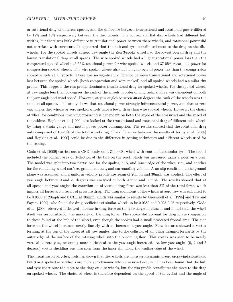
CHAPTER 3. LITERATURE REVIEW 70
or rotational drag at di!erent speeds, and the di!erence between translational and rotational power di!eredby 12% and 40% respectively between the disc wheels. The convex and flat disc wheels had di!erent hubwidths, but there was little di!erence in translational power between these wheels, and rotational power didnot correlate with curvature. It appearred that the hub and tyre contributed most to the drag on the discwheels. For the spoked wheels at zero yaw angle the Zen 3-spoke wheel had the lowest overall drag and thelowest translational drag at all speeds. The wire spoked wheels had a higher rotational power loss than thecompressed spoked wheels; 45-55% rotational power for wire spoked wheels and 37-55% rotational power forcompression spoked wheels. The wire spoked wheels also had a higher overall power loss than the compressionspoked wheels at all speeds. There was no significant di!erence between translational and rotational powerloss between the spoked wheels (both compression and wire spoked) and all spoked wheels had a similar rimprofile. This suggests the rim profile dominates translational drag for spoked wheels. For the spoked wheelsat yaw angles less than 30 degrees the rank of the wheels in order of longitudinal force was dependent on boththe yaw angle and wind speed. However, at yaw angles between 40-50 degrees the rank of the wheels was thesame at all speeds. This study shows that rotational power strongly influences total power, and that at zeroyaw angles disc wheels or aero spoked wheels have a lower drag than wire spoked wheels. However, the choiceof wheel for conditions involving crosswind is dependent on both the angle of the crosswind and the speed ofthe athlete. Hopkins et al. [1990] also looked at the translational and rotational drag of di!erent bike wheelsby using a strain gauge and motor power power consumption. The results showed that the rotational dragonly comprised of 10-20% of the total wheel drag. The di!erences between the results of Jermy et al. [2008]and Hopkins et al. [1990] could be due to the di!erence in testing techniques and di!erent wheels used forthe testing.
Godo et al. [2009] carried out a CFD study on a Zipp 404 wheel with continental tubular tyre. The modelincluded the contact area of deflection of the tyre on the road, which was measured using a rider on a bike.The model was split into two parts: one for the spokes, hub, and inner edge of the wheel rim, and anotherfor the remaining wheel surface, ground contact, and surrounding volume. A no slip condition at the groundplane was assumed, and a uniform velocity profile upstream of 20mph and 30mph was applied. The e!ect ofyaw angle between 0 and 20 degrees was analysed at both 20mph and 30mph. The results showed that atall speeds and yaw angles the contribution of viscous drag force was less than 3% of the total force, whichimplies all forces are a result of pressure drag. The drag coe"cient of the wheels at zero yaw was calculted tobe 0.0308 at 20mph and 0.0311 at 30mph, which was similar to results by Greenwell et al. [1995] and Tew andSayers [1999], who found the drag coe"cient of similar wheels to be 0.0389 and 0.028-0.03 respectively. Godoet al. [2009] observed a delayed increase in drag force as the yaw angle increased, and found that the wheelitself was responsible for the majority of the drag force. The spokes did account for drag forces comparibleto those found at the hub of the wheel, even though the spokes had a small projected frontal area. The sideforce on the wheel increased nearly linearly with an increase in yaw angle. Flow features showed a vortexforming at the top of the wheel at all yaw angles, due to the collision of air being dragged forwards by theouter edge of the surface of the rotating wheel into the oncoming flow. This vortex was seen to be nearlyvertical at zero yaw, becoming more horizontal as the yaw angle increased. At low yaw angles (0, 2 and 5degrees) vortex shedding was also seen from the inner rim along the leading edge of the wheel.
The literature on bicycle wheels has shown that disc wheels are more aerodynamic in zero crosswind situations,but 3 or 4 spoked aero wheels are more aerodynamic when crosswind occurs. It has been found that the huband tyre contribute the most to the drag on disc wheels, but the rim profile contributes the most to the dragon spoked wheels. The choice of wheel is therefore dependent on the speed of the cyclist and the angle of

CHAPTER 3. LITERATURE REVIEW 71
the crosswind. Although there is some variability between the contribution of rotational drag to the overalldrag on bicycle wheels, it is clear that pressure drag is the dominant force.
3.2.2.8 Air density and Altitude
A reduction in air density causes a reduction in aerodynamic drag due to the fewer air particles per squaremeter. Air density is calculated by using the ambient temperature, pressure, and relative humidity, as shownby Equation 3.25, where Pd is the partial pressure of dry air (Pa), Pv is the partial pressure of wet air (Pa),Rd is the specific gas constant for dry air (JK!1kg!1), Rv is the specific gas constant for wet air (JK!1kg!1),T is the temperature (K), # is the relative humidity, and Psat is the saturation vapour pressure of water (Pa).
" =Pd
RdT+
Pv
RvT(3.25)
Pd = P ! Pv (3.26)
Pv = #Psat (3.27)
Psat = 610.78" 10(7.5T!2048.625/T!35.85) (3.28)
Equation 3.25 can be used to show that:
• An increase or decrease in temperature by 3°C causes a decrease or increase in air density by 2%respectively.
• An increase or decrease in relative humidity by 5% causes a decrease or increase in air density by 0.5%respectively.
• An increase or decrease in pressure by 1KPa causes an increase or decrease in air density by 1%respectively.
• An increase in temperature by 3°C and a decrease in pressure by 2KPa causes the air density to bereduced by 4%.
• It should be noted that a 2% reduction in air density is equivalent to a 0.57s reduction in finishing time.
These results are similar to those reported by Di Prampero et al. [1979] and Atkinson et al. [2003], who suggestthat a change in temperature by 3°C will cause a change in drag by 1%, and an increase in temperature by3°C and a decrease in pressure by 2KPa will cause a reduction in air density, and therefore drag, by 4%.These results show that temperature and pressure have a significant e!ect on air density, and therefore drag,but relative humidity has a much smaller e!ect. However, it should be noted that relative humidity canchange by a much greater amount (>50%) than absolute temperature (<10%) from race to race.
The air density, and therefore drag, also reduces with an increase in altitude, enabling athletes to pedal fasterfor the same amount of power output. According to Wilber [2003] the optimal altitude for cycling between

CHAPTER 3. LITERATURE REVIEW 72
2km and 40km time trials is 3200m to 3500m, resulting in a reduction in finishing time by approximately 4%compared to sea level. Although at such high altitudes VO2max is significantly reduced, the improvement incycling aerodynamics exceeds the reduction in VO2max, resulting in faster cycling speeds at altitude [Wilber,2003].
Di Prampero [2000] suggests the relative gain in speed for a cyclist riding at altitude can be predicted byEquation 3.29, where Va is the velocity at altitude (m/s), V1 is the cycling speed at measured conditions(m/s), A is the fractional decrease of VO2max, and k is the fractional decrease of energy expenditure per unitdistance due to altitude. However, Equation 3.29 assumes that athletes can maintain the same VO2max ataltitude as they can at sea level, which is not strictly true.
Va
V1= 3
'A/k (3.29)
3.2.2.9 Summary
The review of literature on the factors that a!ect the aerodynamic drag of cycling has shown that athleteposition is by far the most significant factor, with a low, crouched position that reduces the frontal area beingthe most advantageous for individual riders. When multiple riders are considered, drafting can significantlyreduce the aerodynamic drag of both leading and drafting riders, although this benefit is lost once the spacingbetween riders exceed about 3m. The priority for athletes and coaches looking to gain a competitive advantageshould therefore be optimising athlete position in order to reduce the aerodynamic drag and maximise cyclingspeed. Once position has been optimised, the focus can then turn to improvements in the frame and wheeldesign, the choice of helmet, pedals, footwear, and clothing, and then to making improvements to the designof clothing to consider surface roughness, trips, dimples, and zoned fabric. It is impossible to have anyexternal influence on the air density and altitude at which races take place, and although athletes can trainin extreme conditions to maintain the same VO2max at altitude as they can at sea level, altitude and airdensity can be considered dependent variables.
The literature has shown that the drag of bike frames and wheels has already reached a point where onlyminimal gains can be made through further changes in their design. Therefore the focus of this thesis willconcentrate primarily on individual athlete position, followed by an analysis of helmets, pedals, skinsuitdesign, and fabric choice.

Chapter 4
Mathematical Model of the IndividualPursuit
Introduction
Presented in this section is a mathematical model for the Individual Pursuit (IP) event for track cycling onan indoor velodrome. This model takes into account leaning in the bends and the actual position of the rideron the track by using data collected by the SRM training system. As mentioned in Chapter 2 (Background)performance in track cycling is e!ectively only dependent on factors which a!ect power supply and powerdemand, and the overall aim of competitive track cycling is to minimise the demand of power so that lesspower output is needed to match this demand and as little energy as possible is wasted. As the interactionbetween the power supplied by the rider and the bike is direct, any excess power produced by the athlete willresult in acceleration of the system; the larger the excess power the greater the acceleration and the faster thefinishing time. This mathematical model uses supply and demand equations to determine the surplus powerof an IP athlete for a particular race, and assumes this surplus power leads to acceleration of the centre ofmass of the rider.
The optimal path for the IP is to follow the black line, as this is the shortest distance around the track.However, it is almost impossible for athletes to follow this path exactly, so the actual distanced travelled bythe athlete is likely to be slightly greater than the race distance. Although there is a small discrepency betweenthe actual distanced travelled and the race distance, the mathematical model is based on the assumptionthat athletes follow the black line, as this value is known.
The mathematical model will be used to analyse the e!ect of changing a number of variables on the predictedfinishing time, and for generating theoretical pacing strategies in order to identify the optimal pacing strategyfor IP athletes.
Although the model is similar to those created by Lukes et al. [2005] and Martin et al. [2006], it is uniquein the way that it is designed specifically for track cycling, uses actual SRM power data rather than averagepower or generated power profiles, uses actual velodrome data and does not assume a circular track, includesseparate losses for tyres and bearings, and the equations used to form the mathematical model are describedin terms of power rather than force, as this is more appropriate measure of cycling intensity.
73

CHAPTER 4. MATHEMATICAL MODEL OF THE INDIVIDUAL PURSUIT 74
4.1 Fundamental Equations
Assuming that the bike and rider are one system, the Free Body Diagram (FBD) of the forces acting on thesystem on a banked velodrome track can be shown by Figure 4.1, where FD is the aerodynamic drag force(N), FA is the force to overcome acceleration or deceleration of the bike (N), FT is the transmitted forceas a result of the power supplied by the athlete (N), FR is the rolling resistance (N) where r denotes therear wheel and f denotes the front wheel, FN is the normal force at the point of contact between the wheeland track (N) where r denotes the rear wheel and f denotes the front wheel, FF is the lateral friction forcebetween the wheels and track (N), FC is the centripetal force (N), m is the mass of the bike and rider system(kg), g is the acceleration due to gravity (m/s2), COM is the centre of mass of the system, ! is the leaningangle (rads), + is the gradient of the track (rad), and & is the banking angle of the track (rad). H is theheight of the seat (m).
(a) Side view (b) Rear view
Figure 4.1: Free body diagram of the forces acting on a bike and rider system
Resolving forces in Figure 4.1a in the horizontal direction gives:
FA = mgsin+ + FT ! FD ! FNsin+ ! FRcos+ (4.1)
and in the vertical direction gives:
FNcos+ = mg + FRsin+ (4.2)
Resolving forces in Figure 4.1b in the horizontal direction gives:
FF cos& + FNsin& = FC (4.3)
and in the vertical direction gives:

CHAPTER 4. MATHEMATICAL MODEL OF THE INDIVIDUAL PURSUIT 75
FNcos& = mg + FF sin& (4.4)
Although it is possible that there is a very slight grade angle (+) on the track when riding on the blackline, it will be assumed that + = 0 for simplicity, and also because the velodrome is a symmetrical trackand any slight incline will be o!set by a decline at the same angle. This will simplify Equation 4.1 toFA = FR ! FD ! FR, and Equation 4.2 to FN = mg.
4.1.1 Power
Power is a more appropriate measure of cycling intensity than velocity because power takes into account theamount of work delivered per unit of time. Knowing that Force = Power" V elocity, the power required byan athlete to produce a force to overcome resistance for a given velocity, V, can be determined. Thereforethe following equations used to form a mathematical model of the IP will be described in terms of power.
4.1.2 Demand Side Equations
4.1.2.1 Power to Overcome Aerodynamic Drag Force (FD)
The aerodynamic drag accounts for the majority of the resistance acting on the bike and rider system.Assuming still air inside a velodrome (i.e. zero wind speed) the velocity of the air over the bike and ridersystem is equal to the velocity of the bike. The power required to overcome the aerodynamic drag force, FD
can therefore be written as:
PD =1
2"CdAV 3 (4.5)
where " is the air density (kg/m3), Cd is the drag coe"cient, A is the frontal area of the system (m2), andV is the velocity of the system (m/s).
4.1.2.2 Power to Overcome Tyre Rolling Resistance (FR)
Rolling resistance is the resistance to a wheel’s steady motion, caused by power absorption in the surfacesof the wheel and surface on which it rolls [Wilson, 2004, p208]. Typical values of the coe"cient of rollingresistance, Crr, range from 0.002 to 0.010 for bicycle tyres, depending on track surface, cycling velocity,tyre inflation pressure, wheel diameter, tyre thickness, tyre material, inner tube material, tyre-rim interface,steering angle, temperature, and lean of bike [Wilson, 2004, p211]. A value of Crr = 0.002 was used for thecoe"cient of tyre rolling resistance in the mathematical model because the model was created primarily forelite, track cyclists who would be at the most e"cient end of the scale due to their narrow, smooth tyresinflated to high pressures, and the hard, wooden surface of indoor velodromes on which they race.
According to Kyle [2003a] tyre rolling resistance increases when cornering, primarily because the tyre deformslaterally to set up an elastic stress which provides the centripetal acceleration. Tyre rolling resistance increasesfurther if steering (scrubbing) occurs. As the track is always banked on a velodrome, Kyle [2003a] foundathletes adjust the steering angle by 1° in the straights and 4° in the bends. This corresponds to a 4.1%

CHAPTER 4. MATHEMATICAL MODEL OF THE INDIVIDUAL PURSUIT 76
and 28.6% increase in tyre rolling resistance in the straights and bends respectively, as shown in Figure 4.2.A scrubbing factor, Cs, should therefore be included in the calculation of power to overcome tyre rollingresistance, where Cs=1.04 in the straights and Cs=1.28 in the bends.
Figure 4.2: Increase in rolling resistance due to steering angle
The power required to overcome tyre rolling resistance can be written as:
Prr = (FNCrrV Cs) cos&cos+ (4.6)
where FN is the normal force acting on the wheel (N), Crr is the coe"cient of rolling resistance, V is thevelocity of the system (m/s), & is the banking angle (rad), and + is the gradient of the track (rad).
As it is assumed that + = 0, the power required to overcome tyre rolling resistance can be simplified toPrr = (FNCrrV Cs) cos&.
4.1.2.3 Power to Overcome Bearing Rolling Resistance
There is a small resistance from the bearing seals around the axle of a bike caused by the scrubbing motionof the rolling elements, which should not be ignored. Typical values for the coe"cient of bearing rollingresistance, Cbr, are less than 0.001 [Wilson, 2004, p214], so Cbr = 0.001 was used in the model for eachbearing. The power required to overcome bearing rolling resistance can be written as:
Pbr = FNCbrrb(cos&cos+ (4.7)

CHAPTER 4. MATHEMATICAL MODEL OF THE INDIVIDUAL PURSUIT 77
where Cbr is the coe"cient of bearing rolling resistance, rb is the bearing radius (m), ( is the wheel rotationalspeed (rad/s), & is the banking angle (rad), and + is the gradient of the track (rad).
As it is assumed that + = 0, the power to overcome bearing rolling resistance can be simplified to Pbr =
FNCbrrb(cos&.
4.1.2.4 Power to Overcome Weight Resistance
The power to overcome resistance from the weight of rider, bike frame and the wheels, assuming + = 0, canbe expressed as:
Pg = mgV (4.8)
where m is the mass of the whole system (kg), g is the acceleration due to gravity (m/s2), and V is thevelocity of the system (m/s).
4.1.2.5 Power to Overcome Wheel Aerodynamic Resistance
The aerodynamic drag of bike wheels has been studied since the early 20th Century [Jermy et al., 2008].Wind tunnel tests are often used to determine the drag area of cyclists, but it is not always the case that cyclerigs for wind tunnel testing enable both the front and rear wheels to be rotating. For cases when the frontwheel is stationary, the aerodynamic power term associated with rotating wheels is not measured. Thereforeby calculating the power required to overcome wheel resistance separately from the aerodynamic resistanceof the bike frame and rider (excluding both wheels) a more accurate model can be created. Jermy et al.[2008] describe the method by which they determine the aerodynamic drag on both spoked and disc wheels,leading to the following equation for the power required to overcome this resistance depending on the typeof wheel used, where $ , ' and , are the coe"cients used to fit a quadratic to the power absorbed by thedrag of the wheel ($ = 0.2118, ' = !0.7388, , = 0 [Jermy et al., 2008]). Wheel drag is assumed to be zeroat low velocities, as wheel drag cannot be negative.
Pw = $V 2 + 'V + , (4.9)
For cases where wind tunnel tests of cyclists include both the front and rear wheel rotating, the power termassociated with rotating wheels is measured so Equation 4.9 can be eliminated, providing that the calculateddrag area, CdA, includes the rider, frame and both wheels.
4.1.3 Supply Side Equations
4.1.3.1 Power Produced by the Athlete (Transmitted Force (FT ))
Some of the power supplied by the athlete will be lost due to ine"ciencies of the bike. These include drivechain losses, sti!ness losses, and bearing losses. These losses are minimal compared to aerodynamic resistance,however, they should not be ignored. Therefore, the total power transmitted by the athlete can be expressedas:

CHAPTER 4. MATHEMATICAL MODEL OF THE INDIVIDUAL PURSUIT 78
PT = -Pinput (4.10)
where Pinput is the instantaneous power supplied by the athlete (W), and - is the e"ciency of the bike.
Drive chain e"ciency has been shown to be 95-98% e"cient [Kyle, 2003a], and for elite, track racing cycliststhe e"ciency will be at the higher end of the scale as there are no gears, the chain will be well lubricatedand aligned, and the athletes will pedal fast. Therefore the drive chain e"ciency for the mathematical modelwas chosen to be 98% e"cient.
The instantaneous power supplied was input into the model by using SRM data taken for a specific race foran individual athlete. This allows the actual position of the rider on the track to be accounted for, as thepower output will vary depending on whether the rider is in the bends or straights. The SRM training systemlogs power output every 0.5 seconds. The instantaneous power is determined by a linear interpolation of twoSRM power readings taken 0.5 seconds apart, as shown in Equation 4.11 and Table 4.1, where P i
athlete is theinstantaneous power produced by the athlete (W), ti is the instantaneous time (s), P p
i and tpi are the poweroutput (W) and time (s) at the previous SRM reading, and P s
i and tsi are the power output (W) and time(s) at the subsequent SRM reading.
P iathlete = P p
i +ti ! tpitsi ! tpi
(P si ! P p
i ) (4.11)
ti tpi P pi tsi P s
i P iathlete
0 0 0.00001 0.5 657 0.000010.005 0 0.00001 0.5 657 6.570.01 0 0.00001 0.5 657 13.150.015 0 0.00001 0.5 657 19.730.02 0 0.00001 0.5 657 26.30
Table 4.1: Interpolation of SRM power data
4.1.4 Power Associated with Acceleration or Deceleration of the Bike (FA)
The power required to overcome acceleration or deceleration of the bike can be split into separate terms; onefor the wheels of the bike, and another for the legs of the athlete. The power to overcome the acceleration ofthe wheels arises from translational motion based on the translational velocity (Equation 4.12) and rotationalmotion based on moments of inertia and wheel radius (Equation 4.13), where Pt is the power to overcometranslational acceleration of the wheels (W), m is the mass of the whole system (kg), V is the velocity ofthe system (m/s), Pr is the power to overcome rotational acceleration of the wheels (W), ( is the angularvelocity (rad/s), I is the moment of inertia of the wheels (kg/m2), and rw is the radius of the wheel (m).
Pt = mV (4.12)

CHAPTER 4. MATHEMATICAL MODEL OF THE INDIVIDUAL PURSUIT 79
Pr = I(
rw(4.13)
The legs can be subdivided into thighs, calves and feet, each of which has its own mass, radius of gyration,and moment of inertia. Therefore the total power required to overcome acceleration from the legs can bewritten as PL = PTh + PCa + PF , where:
PTh = IThC
rgTh(4.14)
PCa = ICaC
rgCa(4.15)
PF = IFC
rgF(4.16)
where PL, PTh, PCa, and PF are the powers required to overcome acceleration of the legs, thighs, calves andfeet respectively (W), I is the moment of inertia (kg/m2) where Th, Ca and F represent the thighs, calvesand feet respectively, C is the pedalling cadence (rpm), and rg is the radius of gyration (rad/s) where Th,Ca and F represent the thighs, calves and feet respectively.
The pedalling cadence, C, is the ratio of the rear wheel rotational speed, (, to the gear ratio:
C =(
gearing(4.17)
In order to determine the moment of inertia and radius of gyration of the legs, two athletes (one male 1.93min height and 82kg in weight, and one female 1.68m in height and 59kg in weight) were asked to pedal on abike fixed to the cycle rig so that their pedal strokes could be captured by high speed video. Markers wereplaced on the foot, calf and thigh, as shown in Figure 4.3, and the athletes told to pedal at 100rpm for 1minute. The location of the markers was then tracked using Matlab to locate the x and y coordinates ofeach marker in each frame. The coordinates were then plotted for the foot, calf and thigh for each athlete toillustrate the motion of each part of the leg throughout one revolution, as shown in Figures 4.4 and 4.5.

CHAPTER 4. MATHEMATICAL MODEL OF THE INDIVIDUAL PURSUIT 80
Figure 4.3: Location of markers on the foot, calf and thigh
(a) Foot (b) Calf
(c) Thigh
Figure 4.4: Motion of the Foot, Calf and Thigh for the Male Athlete

CHAPTER 4. MATHEMATICAL MODEL OF THE INDIVIDUAL PURSUIT 81
(a) Foot (b) Calf
(c) Thigh
Figure 4.5: Motion of the Foot, Calf and Thigh for the Female Athlete
The motion of the foot and calf is similar to that of an ellipsoid, where the radius of gyration can be expressedby Equation 4.18, where a and b are the distances from the centre of the ellipsoid in the horizontal and verticaldirections respectively. The motion of the thigh is similar to a pendulum, where the radius of gyration isequal to the length of the thigh.
rofoot =1
2
'(a2 + b2) (4.18)
The moment of inertia for both ellipsoids and pendulums can be expressed by Equation 4.19.
I = mr2o (4.19)
The lengths of the leg segments for the two athletes were measured, and the mass of each segment calculatedby multiplying the total body mass by the average ratio of segment mass to total body mass [Drillis et al.,1964]. The radius of gyration and moment of inertia for the two athletes were calcluated using Figure 4.4and Equations 4.18 and 4.19, and the average values calculated for a rider of 75kg body mass. These averagevalues (Table 4.2) were inserted into the mathematical model to calculate the power required to overcomeacceleration of the legs.

CHAPTER 4. MATHEMATICAL MODEL OF THE INDIVIDUAL PURSUIT 82
Segment Mass to Total Mass (%) Mass (kg) Radius of Gyration (m) Moment of Inertia (kgm2)Foot 2.75 2.0625 0.107 0.0238Calf 9.49 7.1175 0.083 0.0484
Thigh 25.11 18.83 0.366 2.5227
Table 4.2: Average mass, radius of gyration, and moment of inertia data for a 75kg human [Drillis et al.,1964]
4.1.5 Governing Equation
The mathematical model is generated by calculating the surplus power from total power supplied minustotal power demand, and then equating acceleration to surplus power; in other words it is assumed that anyadditional power supplied results in acceleration of the centre of mass. The power equation is initially solvedto determine acceleration in terms of current velocity (a = dV
dt ) and once the initial acceleration has beencalculated it is possible to calculate the new velocity for a small increment, which in turn updates the powerequation to yield a new value for dV/dt. A description of the complete calculation process can be seen inSection 4.1.8.
4.1.6 Additional Parameters
4.1.6.1 Motion in the Bends and Straights
In order to prevent a bike from tipping, the FBD must be balanced. For steady, horizontal motion this willbe when the COM is vertically above the seat of the bike. However, when travelling around a bend or duringan acceleration phase, the combination of the vertical, gravitational force and horizontal, centripetal force(the elastic force in the laterally deformed tyre) results in a tipping angle, as shown in Figure 4.6a. Thisresults in the centre of mass travelling a shorter distance than the wheels when in the bends, as shown inFigure 4.6b.

CHAPTER 4. MATHEMATICAL MODEL OF THE INDIVIDUAL PURSUIT 83
(a) Tipping of the bike when travellingaround a bend or during an accelerationphase
(b) Path of the wheels and COM
Figure 4.6: Motion in the bends
The radius of curvature of the COM, rcom, can be expressed in terms of the radius of curvature of the wheels,rw, as shown in Equation 4.20, where H is the distance of the COM from the contact point between thewheels and track surface (m), and ! is the leaning angle (rad).
rcom = rw !Hsin! (4.20)
The leaning angle, !, can be determined by resolving forces acting on the COM, as shown in Figure 4.7 andEquation 4.21, where m is the mass of the system (kg), Vw is the velocity of the wheels (m/s), rCOM is theradius of curvature of the centre of mass (m), and g is the gravitational acceleration (m/s2).
Figure 4.7: Leaning angle
tan! =mV 2
w
rcommg
! = tan!1
"V 2w
rcomg
#(4.21)

CHAPTER 4. MATHEMATICAL MODEL OF THE INDIVIDUAL PURSUIT 84
As both equations 4.20 and 4.21 include terms for the lean angle and radius of curvature of the COM, aniterative procedure is used to determine appropriate values for the lean angle and radius of curvature of thecentre of mass; assuming initially that rcom = rw, an initial approximation of the lean angle, !, can be foundusing Equation 4.21, which is then used to give an improved value for rcom. This process is repeated threetimes in order to find suitable values for rcom and !; trial and error identified that any more than threeiterations did not reduce the finishing time any more, as shown in Figure 4.8.
Figure 4.8: The dependence of the finishing time on the iterative procedure for the leaning angle and radiusof curvature of the centre of mass
4.1.6.2 Normal Force Acting on the Wheels and Bearings
By taking moments about the COM from Figure 4.1b, the normal force, FN , can be determined:
FNHsin! = FFHsin(*2! ! ! 2&
)(4.22)
orFF =
FNsin!
sin*$2 ! ! ! 2&
+
and from Equation 4.22, FF can be eliminated:
FN =mgsin
*$2 ! ! ! 2&
+
cos&sin*$2 ! ! ! 2&
+! sin!sin&
(4.23)

CHAPTER 4. MATHEMATICAL MODEL OF THE INDIVIDUAL PURSUIT 85
4.1.6.3 Air Density
The air density was calculated using Equation 4.24 for air density for moist air described by Davis [1992],where p is the pressure (Pa), Ma is the molar mass of dry air, xv is the mole fraction of water vapour, T isthe temperature (K), R is the molar gas constant, Mv is the molar mass of water, and Z is the compressibilityfactor.
" =pMa
ZRT
!1! xv
"1! Mv
Ma
#$(4.24)
At a lower air density the aerodynamic drag decreases, and therefore athletes can pedal faster for the sameamount of power output. However, there is also a decline in maximal oxygen uptake, VO2max, when the airdensity is lower (at higher altitudes) and although athletes can acclimatise to such conditions, a decreasein VO2max will lead to a decrease in power output. The decline in power output can be assumed to beequivalent to the decline in VO2max, and for an acclimatised subject this can be described by Equation 4.25[Davis, 1992].
P = (!1.122)x2 ! (1.8991)x+ 99.921 (4.25)
Equation 4.25 is useful for estimating finishing times for an athlete on di!erent indoor velodromes, especiallywhen the only available instantaneous power output data is from one specific velodrome.
The temperature was taken from SRM data, and the atmospheric pressure and relative humidity taken fromrecorded data for the closest airport to the velodrome on which the race was taking place [Underground,2009]. Although climatic conditions are often controlled in velodromes, this was the most consistent methodof obtaining atmospheric data for each athlete without actually being present at the race.
4.1.6.4 Frontal Area
The drag coe"cient and frontal area of the system both depend on the shape of the body involved, so can becombined as a single variable for drag area. The overall drag area, CdA, was determined from wind tunnel dataand the frontal area of the rider, bike and wheels was determined using the digitizing method, as describedin Section 5.1.2.2, during the wind tunnel tests. As the wind tunnel tests carried out at the University ofCanterbury do not allow rotation of the front wheel, it is necessary to include the term for power to overcomewheel resistance, which has already been described in Section 4.1.2.5. In order to avoid accounting for thewheel drag twice, the drag area for the athlete and bike, excluding the wheels, was determined and this valueused in Equation 4.5 to determine the power required to overcome aerodynamic drag.
CdArider+bike = CdArider+bike+wheelsArider+bike+wheels !Awheels
Arider+bike+wheels(4.26)
Equation 4.26 and the separate contribution for wheel drag could be omitted, but this would mean all theinformation on wheel and rider drag comes from one drag area measurement in the wind tunnel. Althoughthis is more simple, wheel rotational aerodynamic resistance would not be accounted for those wind tunneltests carried out at the University of Canterbury.

CHAPTER 4. MATHEMATICAL MODEL OF THE INDIVIDUAL PURSUIT 86
For athletes not tested in a wind tunnel, the drag area, CdA, can be determined by calculating the quantitiesfor the left and right sides of Equation 4.27 using SRM data, and using linear regression to determine thedrag area for a constant coe"cient of friction [Martin et al., 2006]. This equation includes wheel drag, so itis not necessary to include the extra term for power to overcome wheel resistance (Equation 4.9) in this case.
CdA1
2"V 3 + µFNV = Pav " Efficiency ! 'KE
't! 'PE
't!mgCrrV (4.27)
where Pav is the average power from SRM data (W), $KE$t is the change in kinetic energy of the system over
the total finishing time (J/s), $PE$t is the change in potential energy of the system over the total finishing
time (J/s), " is the air density (kg/m3), V is the average velocity (m/s), µ is the coe"cient of friction, FN
is the normal force (N), m is the total mass of the system (kg), g is the acceleration due to gravity (m/s2),and Crr is the coe"cient of rolling resistance.
4.1.6.5 Initial Velocity
Although in reality the initial velocity is zero, the mathematical model requires a positive initial velocityto be stated to prevent the governing equation from tending to infinity as the velocity tends to zero. Aninitial velocity that is too high will generate an artificial surge at the start of the mathematical model, so inorder to determine the optimal initial velocity the dependence of the initial velocity on the finishing time wasexplored. It was found that an initial velocity of 0.0003kph provided the smallest starting velocity withoutgenerating an artifical surge, and also resulted in the most accurate predicted finishing time, as shown inTable 4.3. Details of all other parameters used to identify the optimal initial velocity are given in Table 4.4.
Predicted Finishing Time (s)Initial Velocity (kph) Athlete 11 (Actual T=265.023s) Athlete 6 (Actual T=267.566s)
0.0002 223.038 224.8450.0003 264.887 267.6120.0004 266.859 269.5970.0005 267.597 270.3020.0006 267.937 270.6250.0007 268.122 270.7960.0008 268.230 270.9000.0009 268.301 270.9650.0010 268.349 271.010
Table 4.3: E!ect of initial velocity on the finishing time

CHAPTER 4. MATHEMATICAL MODEL OF THE INDIVIDUAL PURSUIT 87
Athlete Data Wheel Data (each wheel)Height (m) 1.85 Power coe"cient ! 0.2118Weight (kg) 75 Power coe"cient " -0.7388CdA (m2) 0.198 Power coe"cient # 0
Race distance (m) 4000 Crr tyre 0.001Crrbearing 0.001
Track Data Environmental DataLap distance (m) 250 Temperature (˚C) 24
Banking angle straights (rad) 0.22 Pressure (mbar) 1016.86Banking angle bends (rad) 0.733 Relative humidity (%) 56
Radius of curvature straights (m) 1x10²¹Radius of curvature bends (m) 26.101
Table 4.4: Parameters used to determine the optimal initial velocity
4.1.6.6 Time Step
A first order Euler time integration technique was used to determine the finishing time, where the equationsdescribed above were solved at every time step starting from t=0s. The time step should be small enough sothe results don’t change, but a time step which is too small will take longer for the equations to be solved.The mathematical model was generated in Microsoft Excel, which has a limit to the number of iterationsthat can be performed. Therefore, the smallest possible timestep which could be used for the model in Excelwas dt=0.005s.
4.1.6.7 Accounting for SRM Delay
The SRM Training System does not start recording data until one complete revolution, causing a delay atthe start of approximately 3 seconds. In order to account for this delay, a linear interpolation was appliedbetween zero and the first recorded power output, so that the first recorded power output was input into themodel at 3 seconds, as shown in Table 4.5.
Time (s) Power (W)0 0.0001
0.5 1081 216
1.5 3252 433
2.5 5413 649*
Table 4.5: Interpolation of initial power recorded by SRM* This is the first recorded power output by the SRM.

CHAPTER 4. MATHEMATICAL MODEL OF THE INDIVIDUAL PURSUIT 88
4.1.7 Assumptions
1. Sti!ness losses are combined with drive train losses, which have been approximated as a reduction ininstantaneous power output by 2%, and drive train losses do not vary with power output.
2. All types of bearing losses are incorporated into losses due to bearing rolling resistance.
3. Tyre rolling resistance increases by 4.1% in the straights and 28.6% in the bends.
4. Grade angle is assumed to be zero.
5. About 40% of the weight of the frame acts on the front wheel and bearings; the remaining 60% actson the rear wheel and bearings. Therefore, the normal force acting on the front and rear wheels andbearings will be 40% and 60% of Equation 4.23 respectively.
6. The rear wheel dissipates only 60% of the power of the isolated front wheel due to shielding by theframe [Jermy et al., 2008].
7. The centre of mass is taken to be equal to the height of the seat, measured vertically from the ground.The mathematical model is relatively insensitive to the centre of mass position, and a method toestimate the centre of mass of a seated bike and rider was developed by Moore et al. (2009), givingthe location of the centre of mass for a 75kg rider to be 1.06m vertically from the ground, which iscomparable to seat heights of 1-1.2m used for the mathematical model.
8. There is negligible e!ect of wind on an indoor velodrome, as on a circular, symmetrical track any headand tail winds cancel each other out. This eliminates any equations for sidewind, which would beapplicable in a mathematical model for road cycling.
9. The coe"cient of rolling resistance does not vary with velocity, tyre or track surface.
10. The athlete travels on the black line throughout the event.
4.1.8 Calculation Procedure
The model was compiled in a Microsoft Excel Spreadsheet, and the calculation procedure used a time-steppingtechnique where by the equations were solved in a certain order at every time-step starting from t=0s. Thecalculations were performed in the following order:
1. Calculate the initial acceleration
For an initial velocity of 0.0003kph, the power to overcome losses, Plosses , the instant power produced bythe athlete, P i
athlete, and the power to overcome acceleration, P acceleration, can be determined at t=0s. Theinitial acceleration can then be determined by:
a =Psurplus
Pacceleration(4.28)
where P surplus = P iathlete ! Plosses.
2. Calculate the change in velocity, the velocity of the centre of mass and velocity of the wheels

CHAPTER 4. MATHEMATICAL MODEL OF THE INDIVIDUAL PURSUIT 89
Once the initial acceleration has been determined, the change in velocity can be calculated by dV = a!t.It is assumed that the surplus power leads to acceleration of the centre of mass, so the calculated changein velocity is the change in velocity of the centre of mass. The velocity of the centre of mass at the nexttime-step can then be determined using the velocity at the the previous time-step plus the calculated changein velocity:
Vi+1 = Vi + dV (4.29)
The velocity of the wheels can be determined by:
Vw =Vcom
rcom" rw (4.30)
where V is the velocity (ms!1), r is the radius of curvature (m), w represents the wheels and com representsthe centre of mass.
3. Calculate the distance of the centre of mass and distance of the wheels
The distance travelled by the centre of mass over each time-step is calculated using a discrete version of thekinematic formula d = ut+ 1
2at2, where u = Vi and a(ti+1 ! ti) = dV . The cumulative distance can then be
found by adding the distance travelled over the previous time-step to the total distance travelled until thatpoint, as shown in Equation 4.31.
di+1 = di + Vi(ti+1 ! ti) +dV
2(ti+1 ! ti) (4.31)
The distance of the wheels can then be determined by:
dw =dcomrcom
" rw (4.32)
4. Calculate the finishing time
The finishing time is taken to be the time at which the overall racing distance is reached (3000m for womenIP and 4000m for men IP).
4.1.9 Validation
The accuracy of the mathematical model was determined by comparing finishing times for eleven, IP athletesfor specific World Championship events (five 4000m male races and six 3000m female races). The powerprofile for each athlete was taken from SRM training systems, which were placed on the bike during theevent.
4.1.9.1 Input Parameters
The temperature (°C), pressure (Pa), body weight (kg), athlete height (m), seat height (m) and gear ra-tio were determined for each athlete at the time of the race. The frame, wheel and bearing masses andradii were obtained from the manufacturer, and the velodrome data obtained from the velodrome database

CHAPTER 4. MATHEMATICAL MODEL OF THE INDIVIDUAL PURSUIT 90
(www.fixedgearfever.com). The range of these variables are shown in Table 4.6. The drag area for eachathlete was calculated using Equation 4.27, as not all athletes were able to be tested in the wind tunnel. Thecalculated drag areas are shown in Table 4.7.
Variable Maximum Minimum RangeTemperature (˚C) 28 22 6Pressure (mbar) 1021 1005 16
Relative humidity (%) 60 45 15Body weight (kg) 78.0 54.5 23.5Athlete height (m) 1.90 1.64 0.26
Seat height (m) 1.1 1.0 0.1Gear ratio 3.8 3.2 0.6
Frame mass (kg) 8.0 8.0 0Wheel mass (kg) 1.255 1.145 0.11Wheel radius (m) 0.3315 0.3315 0Bearing radius (m) 0.012 0.012 0
Track banking angle in bends (rad) 0.750 0.733 0.017Track radius of curvature in bends (m) 26.101 26.101 0Track banking angle in straights (rad) 0.22 0.22 0
Track radius of curvature in straights (m) 1x10²¹ 1x10²¹ 0
Table 4.6: Range of variables used in the mathematical model
Athlete1 2 3 4 5 6 7 8 9 10 11
CdA 0.194 0.201 0.195 0.192 0.210 0.174 0.172 0.174 0.209 0.203 0.195
Table 4.7: Calculated drag area for each athlete
The following parameters remained the same for all athletes because all velodromes on which the races tookplace had a lap length of 250m and it was assumed that the grade angle was zero, and the foot, calf and thighparameters were averages determined from video analysis of pedal strokes, as described in Section 4.1.4:

CHAPTER 4. MATHEMATICAL MODEL OF THE INDIVIDUAL PURSUIT 91
ParameterLap length (m) 250
Grade angle (rad) 0Foot mass (kg) 1.0875
Foot radius of gyration (m) 0.10745Foot moment of inertia (kgm2) 0.01256
Calf mass (kg) 3.4875Calf radius of gyration (m) 0.0825
Calf moment of inertia (kgm2) 0.09489Thigh mass (kg) 7.5
Thigh radius of gyration (m) 0.366Thigh moment of inertia (kgm2) 1.00467Wheel moment of inertia (kgm2) 0.065
Coe"cient of tyre rolling resistance (both tyres) 0.002Coe"cient of bearing rolling resistance 0.002
Power coe"cient $ 0.2118Power coe"cient ' -0.7388Power coe"cient , 0
Table 4.8: Input parameters recorded prior to the event
4.1.9.2 Results
A comparison between the predicted finishing time and actual finishing time for each athlete is shown inTable 4.9. These results show that the average di!erence between actual and predicted finishing times is 0.31seconds (0.16%). As the mathematical model under-predicted the finishing time for 6 of the athletes butover-predicted the finishing time for 5 of the athletes there is no clear indication as to whether the model islikely to under or over predict the finishing time for any given athlete.
Athlete Actual finishing time (s) Predicted finishing time (s) Di!erence (s) Di!erence (%)1 222.080 220.583 -1.497 -0.672 221.597 222.064 0.467 0.213 222.990 222.634 -0.356 -0.164 222.819 220.228 -2.591 -1.165 276.640 277.263 0.623 0.236 267.566 267.612 0.046 0.027 233.255 232.695 -0.560 -0.248 267.789 269.747 2.181 0.819 268.118 268.476 0.358 0.1310 215.212 213.306 -1.906 -0.8911 265.023 264.887 -0.136 0.05
RMS 1.30 0.56
Table 4.9: Results of actual and predicted finishing times
A comparison of actual and predicted lap times for Athlete 10 (3000m female race) is shown in Table 4.10.These results show that the greatest error is seen during the first lap, where the model underpredicts the

CHAPTER 4. MATHEMATICAL MODEL OF THE INDIVIDUAL PURSUIT 92
lap time by 3.214 seconds. This could be due to the increased drag area during the standing start in reality,which is not accounted for in the model. It also takes one complete revolution before the SRM TrainingSystem begins to store the data, and although this was accounted for using a linear interpolation betweenzero and the first recorded power output, which was assumed to be at 3 seconds, it would be more realisticto have power data that recorded more frequently than 0.5s intervals. It was also assumed that the riderswould travel exactly 3000m or 4000m during their race, which as previously mentioned would not be exactlytrue, as athletes are not able to stay on the black line throughout the entire race.
Distance (m) Actual Lap Time (s) Predicted Lap Time (s) Di!erence (s)Lap 1 250 23.299 20.085 -3.214Lap 2 500 17.115 17.032 -0.083Lap 3 750 17.615 17.101 -0.514Lap 4 1000 17.873 17.327 -0.546Lap 5 1250 17.796 17.646 -0.150Lap 6 1500 17.674 17.540 -0.134Lap 7 1750 17.726 17.580 -0.146Lap 8 2000 17.831 17.535 -0.296Lap 9 2250 17.958 17.652 -0.306Lap 10 2500 18.191 17.820 -0.371Lap 11 2750 18.209 17.939 -0.270Lap 12 3000 18.239 18.049 -0.190
Table 4.10: Comparison between actual and predicted lap times for Athlete 10
A comparison of the velocity profiles for the predicted velocity of the wheels and the actual velocity recordedby the SRM data for one male and one female athlete (Athlete 11 and Athlete 7) is shown in Figure 4.9. Thisclearly shows the increase in velocity throughout the bends compared to the straights. In general, the modelpredicts a slightly lower velocity in both the bends and straights compared to the SRM data, a di!erence ofapproximately 0.2m/s. The mathematical model tends to underpredict the time to complete the first lap byapproximately 3-4s for each athlete, which is probably due to the increase in aerodynamic drag when athletesstand during the standing start, which is not accounted for in the mathematical model. After the initialacceleration phase, the mathematical model either under-predicts or over-predicts lap times by anythingfrom 0.003s to 0.5s. However, there is no clear trend as to when the model may under or over-predict laptimes, as it appears to vary between athletes.

CHAPTER 4. MATHEMATICAL MODEL OF THE INDIVIDUAL PURSUIT 93
(a) Athlete 11
(b) Athlete 7
Figure 4.9: Comparison of the predicted velocity of the wheels to the actual velocity recorded by the SRMdata
These results show that the mathematical model can be used to predict the finishing time for IP athletes toa high degree of accuracy. Although improvements can be made, such as better atmospheric data and morefrequent power and velocity data, the model is more than capable of being used to predict ’what if’ scenarios

CHAPTER 4. MATHEMATICAL MODEL OF THE INDIVIDUAL PURSUIT 94
without the need for athletes to simulate such conditions on the track.
4.1.10 Relative Contribution of resistive forces
The mathematical model can also be used to identify the relative contribution of the resistive forces to theinstantaneous power output, as shown in Figure 4.10. From Figure 4.10 it is clear to see that the aerodynamicdrag contributes the most to the overall resistive force, with bearing resistance being the minimal resistance.It is also clear that the contribution of all resistive forces varies between the bends and the straights, andthere is a significant increase in resistive forces in the first 20s, which is most likely due to the standingposition of the rider during the standing start. A comparison between the contribution of the resistive forcescalculated from the model and compared to the literature can be seen in Table 4.11. Table 4.11 shows thatthe results are similar between the model and the literature, although the e!ect of scrubbing appears to beslightly greater in the literature. The contribution of bearing rolling resistance calculated in the model tendsto agree with Wilson [2004], who states that the e!ect of bearing rolling resistance is thought to be negligiblecompared to the other resistive forces in cycling. The contribution of aerodynamic drag to overall resistanceis lower in the bends due to the increase in the contribution of rolling resistance and scrubbing, but drag isstill the highest contributor to resistance in both the bends and straights.
Figure 4.10: Contribution of resistive forces

CHAPTER 4. MATHEMATICAL MODEL OF THE INDIVIDUAL PURSUIT 95
Drag Tyre RR Scrubbing Bearing RRStraights 94% 2.5% 0.02% 0.08%Bends 80% 8% 0.7% 0.3%
Literature 90% <10% 0.4% straights [Kyle, 2003a]! negligible [Wilson, 2004](at V>40kph) [Oggiano et al., 2008] [Atkinson et al., 2003] 2.9% bends [Kyle, 2003a]! 2-5% [Martin et al., 2007]
1 to 5% [Wilson, 2004]!
Table 4.11: Contribution of resistive forces as a percentage of instant power* According to Kyle (2003a) scrubbing increases the tyre rolling resistance by 4.1% in the straights and 28.6% in the bends,which is equivalent to 0.4% and 2.9% of the 10% contribution of tyre rolling resistance. Similarly, Wilson (2004) states thatscrubbing can increase the tyre rolling resistance by 10-50%, which is equivalent to 1-5% of the 10% contribution of tyre rollingresistance.
4.1.11 Errors and Improvements
The main source of error is the low frequency of data collection by the SRM system. The SRM only recordsdata every 0.5 seconds, limiting the frequency of the input power for the athlete. In addition, the SRM doesnot start recording data until one complete revolution has been completed, which in turn will cause a delayat the start of the race. Although a linear interpolation was applied for the first three seconds to accountfor this error, it cannot be guaranteed that this represents the actual power output of the athlete for thefirst three seconds. It would be more useful to be able to gather power and data from t=0s and at a highersampling rate.
As mentioned previously, the time-step size and the initial velocity both a!ect the stability and accuracyof the mathematical model. The chosen values were those which produced realistic and stable finishingtimes. Also, the Euler time integration scheme has an inherent error which is related to the timestep. Afuture recommendation would be to trial more accurate time integration schemes, such as the 4th orderRunge-Kutta method, to see if the accuracy of the mathematical model can be improved further.
The pressure and relative humidity data was taken from online weather for the airport closest to the velodromeon which the race was taking place. Climatic conditions are often controlled in velodromes, so althoughthis method of collecting atmospheric data is consistent, it is not as reliable as obtaining real time data.The temperature was taken from SRM data, and it would also be useful to have a similar system thatlogged pressure and relative humidity with the SRM data for future analysis. In addition, more accuratemeasurements of rolling and scrubbing resistance for the tyres used would lead to an improved accuracy forthe mathematical model.
One of the assumptions of the mathematical model was that the overall distance travelled by the athlete wasequal to the race length. However, in reality the athlete is not able to keep to the black line throughout therace, which will cause the cumulative distance travelled to be slightly greater than the race length.
The results shown for the model used a calculated drag area, CdA, rather than a drag area recorded in thewind tunnel. This was because not all athletes had been involved in wind tunnel testing close to the timeof their race, and the drag area has a significant a!ect on the results; if the athlete adopts a very di!erentposition on the day of the race compared to when they were in the wind tunnel, the mathematical modelwould not be as accurate. All IP events have a standing start, where the athlete adopts a standing position

CHAPTER 4. MATHEMATICAL MODEL OF THE INDIVIDUAL PURSUIT 96
for approximately three-quarters of the first lap. This would increase the drag area during this time, whichhas not been included in the model. This is a likely cause of the large di!erence between predicted andactual lap time for the first lap. An improvement on the drag area calculation would be to use the digitizingmethod to calculate the frontal area of an athlete during the race for which the SRM data is collected for.This would ensure the most recent and accurate drag area would be calculated for each athlete, which wouldthen be used for the model. In some cases the bike wheels used for racing were not tested in the wind tunnel,and so only available data for similar wheels could be used in the model. It would be beneficial to build upa database of data for di!erent bike frames and wheels so that users of the model can select the type of bikeand wheels used by the athlete, which would automatically input the relevant data into the model.
4.1.12 E!ect of Changes on Finishing Time
The mathematical model can be used to predict what e!ect changes to model parameters have on cyclingperformance. A number of parameters were reduced by 2% and the finishing time calculated and comparedto the original predicted finishing time. Table 4.12 shows the e!ect of these changes on the finishing time forAthlete 10 (female, 3000m IP athlete, original predicted finishing time 213.306s), categorised into athlete,bike, and environment or track parameters. Note that the seat height changes the position of the centre ofmass but not the drag area in the model, but in reality a change in seat height would also change the dragarea.
Decrease by 2%Input Parameter Predicted Di!erence from
Finishing Time (s) Original Finishing TimeCdA 212.130 -1.176s -0.55%
Seat height 213.306 0.000s 0.00%Athlete Body mass 213.053 -0.253s -0.12%
Athlete height 213.306 0.000s 0.00%Body mass and CdA 211.881 -1.425s -0.67%
Gear ratio 213.318 0.012s 0.01%Tyre rolling resistance 213.243 -0.063s -0.03%
Bike Bearing rolling resistance 213.305 -0.001s 0.00%Wheel radius 213.327 0.021s 0.01%Frame weight 213.274 -0.032s -0.02%Wheel weight 213.296 -0.010s 0.00%Air density 212.092 -1.214s -0.57%
Temperature 213.416 0.110s 0.05%Environment/Track Pressure 212.106 -1.200s -0.57%
Relative humidity 213.320 0.014s 0.01%Banking angle 212.291 -1.015s -0.48%Grade angle* 213.262 -0.044s -0.02%
Table 4.12: E!ect of changes in model parameters on cycling performance* The grade angle was changed to -0.006 for half of a straight section of the track and 0.006 for the otherhalf of a straight section to represent a ’dip’ in the straight sections of the track, which is what may actuallybe experienced by athletes [Palmer, 2009]. This only a!ected the predicted finishing time by 0.044s, so it istherefore acceptable to assume a grade angle of zero throughout the track.

CHAPTER 4. MATHEMATICAL MODEL OF THE INDIVIDUAL PURSUIT 97
The results in Table 4.12 show that a change in drag area, CdA, and body mass together had the mostsignificant e!ect on cycling performance, reducing the finishing time by 0.67%. The reduction in finishingtime from combining these changes was similar to, but slightly greater than the reduction seen from makingthese changes individually. Therefore it should not be assumed that the gains or losses from multiple changesin position are a summation of the individual gains or losses, which would be in agreement with resultspublished by Martin et al. [2006]. Out of all individual changes, air density, drag area, and banking anglehad significant a!ects on the predicted finishing time, with reductions in finishing time of 0.57%, 0.55% and0.48% respectively. However, it should be noted that a 2% reduction in air density is a significant changecompared to a 2% reduction in tyre or bearing rolling resistance. Table 4.12 also shows that changes madeto the athlete and environment/track parameters have a greater e!ect on cycling performance than changesto the bike and components, though of course changes to the environment and track will a!ect all ridersin a given race. This highlights the importance of optimising athlete position in order to maximise cyclingvelocity and performance.
A comparison between a decrease in temperature, pressure and relative humidity shows that changes intemperature have the greatest influence on the air density, with a 1°C decrease in temperature causing theair density to rise by 0.005kgm!3, and therefore increasing the finishing time by 0.248s.
• Decrease in temperature by 1°C = rise in air density by 0.005kgm!3
• Decrease in pressure by 1kPa = reduction in air density by 0.001kgm!3
• Decrease in relative humidity by 1% = rise in air density by 0.001kgm!3
• Decrease in temperature by 1°C and increase in pressure by 1kPa = rise in air density by 0.006kgm!3
Di Prampero et al. [1979] and Atkinson et al. [2003] state that a change in temperature by 3°C is equivalentto a change in drag of 1%. When the mathematical model was used to simulate both an increase and decreasein temperature and drag area by 3°C and 1% respectively (Table 4.13) the results suggested that a changein temperature by 3˚C had a slightly greater e!ect than a change in drag area by 1%.
Change Predicted Finishing Time (s) Di!erence from Original Finishing Time (s)Increase temperature by 3˚C 212.645 -0.661Decrease temperature by 3˚C 213.981 0.675
Increase CdA by 1% 213.915 0.609Decrease CdA by 1% 212.705 -0.601
Table 4.13: E!ect of temperature and drag on cycling performance
4.1.13 Conclusion
The ability to simulate changes to di!erent parameters both individually and together using the mathematicalmodel is a useful tool for both athletes and coaches to help analyse the e!ect of these changes on performance,without the need for these changes to actually be made in reality. The model is also useful for predicting the

CHAPTER 4. MATHEMATICAL MODEL OF THE INDIVIDUAL PURSUIT 98
finishing time for di!erent athletes competing in the same race and conditions; for example a comparison caneasily be made between riders racing on the same velodrome on the same day, but who have di!erent dragareas and masses.
In addition to changes made to the athlete, bike, and environment or track, it is possible to modify thepower output whilst maintaining all other parameters to simulate di!erent strategies and the e!ect of pacingstrategy on performance.
4.2 Optimal Pacing Strategy
The Individual Pursuit (IP) is a closed-loop event, in which athletes must complete a certain distance inthe shortest possible time. The regulation of power output is a clear indication of performance, and pacingprofiles can be analysed to determine the optimal strategy which should be used for a particular race. Highperformance athletes can vary their power output in a number of ways, the choice of which depends on therace distance and the terrain on which the race takes place. According to Abbiss and Laursen [2008] themain types of pacing profiles that have been observed for di!erent forms of exercise in a variety of conditionsare negative, all-out, positive, even, parabolic and variable. A description of these models can be found inthe literature review and in Abbiss and Laursen [2008].
The mathematical model described above was used to simulate di!erent pacing strategies by generatingspecific power profiles that related to those pacing strategies described by Abbiss and Laursen [2008]. Thedata for one of the eleven athletes used for validating the model was used for all other inputs into the model,details of which can be seen in Table 4.14. Each power profile was modified slightly to ensure the overallwork done was the same as that produced during the actual race, so that all generated pacing strategieswere realistic and comparable. Anaerobic reserves are fixed for a given athlete (and deplete to zero in a goodpacing strategy for elite athletes) but whether the aerobic work done increases, decreases, or remains constantfor di!erent pacing strategies is not yet clear. Although it may not necessarily be true that athletes can onlyproduce a certain amount of energy regardless of the pacing strategy used (it is possible that athletes couldincrease their total work done when adopting a specific pacing strategy by increasing the e"ciency with whichanaerobic capacity is used during the race) the assumption that athletes produce the same work done forall pacing strategies enables fair comparions to be made with the information available. The mathematicalmodel also excluded psychological (motivation) e!ects, which may increase the total work output of a riderwhen optimised. A better understanding of athlete fatigue and total work done for di!erent strategies isrequired before being able to included these changes in the model.
The actual finishing time for the race was 265.023s and the predicted finishing time using the mathematicalmodel with actual SRM power data was 264.887s (-0.136s). The maximum power output was 1044W, reachedat 11s into the race, the average power was 466W, and the calculated work done for the entire race was 128.3KJ(work done = sum over all SRM sample of instantaneous power x time interval). An analysis of the powerprofile for the SRM data suggests that the athlete used an all-out strategy for the first 14s of the race, followedby a variable strategy with a higher power output in the bends compared to the straights. The actual SRMpower profile can be seen in Figure 4.11.
According to Abbiss and Laursen [2008] if an athlete’s power or velocity drops below their critical fatiguethreshold or critical power, then performance will be compromised regardless of whether the athlete increasestheir power or velocity during other sections of the race in order to make up for lost time.

CHAPTER 4. MATHEMATICAL MODEL OF THE INDIVIDUAL PURSUIT 99
Athlete Data Environmental DataHeight (m) 1.85 Temperature (°C) 28Weight (kg) 75 Pressure (mbar) 1021CdA (m2) 0.195 Relative humidity (%) 60
Race distance (m) 4000Track Data Frame and Wheel Data (each wheel)
Lap distance (m) 250 Power coe"cient ! 0.2118Grade angle (rad) 0 Power coe"cient " -0.7388
Banking angle straights (rad) 0.22 Power coe"cient # 0Banking angle bends (rad) 0.733 Crr tyre 0.001
Radius of curvature straights (m) 1x10²¹ Crr bearing 0.001Radius of curvature bends (m) 26.101 Wheel radius (m) 0.3315
Front wheel mass (kg) 1.145Rear wheel mass (kg) 1.255
Frame mass (kg) 8
Table 4.14: Rider and bike characteristics used for generating pacing strategies
Figure 4.11: Actual SRM power profile
4.2.1 Negative Pacing Strategy
A negative pacing strategy is one in which athletes show a significant increase in the speed and power towardsthe end of a race (Figure 4.12). It is believed that athletes adopting this strategy use all their anaerobicenergy reserves, as they are aware of the remaining distance for completing the race [Abbiss and Laursen,2008].

CHAPTER 4. MATHEMATICAL MODEL OF THE INDIVIDUAL PURSUIT 100
Figure 4.12: Negative Pacing Strategy
A negative strategy was simulated using the mathematical model by increasing the power to 466W instantlyand maintaining this power until 3500m, at which point the power was increased in a linear fashion from466W to 695W at 4000m (P=0.458d-1137). The simulated negative strategy can be seen in Figure 4.13.
Figure 4.13: Modelling a negative pacing strategy
4.2.2 All-Out Pacing Strategy
For events where the majority of time is spent in the initial acceleration phase it is important for an athleteto maximise their power output during this phase. This is the understanding behind all-out pacing strategies,where a high initial power output is followed by a gradual decline (Figure 4.14).

CHAPTER 4. MATHEMATICAL MODEL OF THE INDIVIDUAL PURSUIT 101
Figure 4.14: All-Out Pacing Strategy
According to Abbiss and Laursen [2008] the initial acceleration phase lasts for approximately 10-20% of thetotal time to complete the race. However, De Koning et al. [1999] state that time at which the change betweenan all-out strategy to an even strategy takes place is critical and depends on anaerobic energy kinetics ofthe athlete. De Koning et al. [1999] suggest that a 12s initial acceleration phase is optimal for the 4000mevent. In order to analyse the length of the initial acceleration phase on the predicted finishing time, aninitial acceleration phase lasting 10s, 12s, 14s, 16s and 18s with a maximum power of 1044W, followed by alinear decrease in power to a final power that resulted in a total work done of 128.3kJ was simulated usingthe mathematical model. A parabolic profile was used for the all-out phase, where the maximum power of1044W was reached in the middle of the all-out phase and the power output at the end of the all-out phasewas 600W, as this was similar to the actual SRM power data and would therefore be realistic. The simulatedall-out strategy with an 14s initial acceleration phase is shown in Figure 4.15.
Figure 4.15: Modelling an all-out pacing strategy
An all-out strategy with a parabolic initial acceleration phase of 10s, 12s, 14s, 16s, and 18s followed by aneven strategy, where the power output during the even phase was such that the total work done was 128.3KJ,was simulated using the mathematical model to identify the e!ect of a linear decrease in power output forthe remainder of the race. The simulated all-out and even strategy is shown in Figure 4.16.

CHAPTER 4. MATHEMATICAL MODEL OF THE INDIVIDUAL PURSUIT 102
Figure 4.16: Modelling an all-out and even strategy
4.2.3 Positive Pacing Strategy
Abbiss and Laursen [2008] describe positive pacing strategies as those with a reduction in speed and heartrate throughout an event, as shown in Figure 4.17. They suggest positive pacing strategies are often adoptedfor races where fatigue is likely to kick in, such as an ironman.
Figure 4.17: Positive Pacing Strategy [Abbiss and Laursen, 2008]
Abbiss and Laursen [2008] suggest a positive pacing strategy is one in which athletes accelerate to 110% ofthe average power for the first 25% of the race, reduces to 98% of the average power for the next 50% of therace, and reduces to 97% of the average power for the remaining 25% of a race (there is a rounding error of<1% which is corrected for by scaling the power to achieve the same work done to within 0.1%. This powerprofile was simulated for the male athlete using the mathematical model, as shown in Figure 4.18, but thepower profile was modified slightly to ensure the total work done was 128.3kJ by setting the power outputto 527W (113% of the average power) for the first 1000m, 471W (101% of the average power) for the next2000m, and 466W (100% of the average power) for the final 1000m.

CHAPTER 4. MATHEMATICAL MODEL OF THE INDIVIDUAL PURSUIT 103
Figure 4.18: Modelling a positive pacing strategy
4.2.4 Even Pacing Strategy
Even pacing strategies are often adopted when the starting strategy has less of an e!ect on performance,due to the smaller percentage of overall time spent in the initial acceleration phase [Abbiss and Laursen,2008]. Such strategies show an initial acceleration to an average velocity and power output, which is thenmaintained for the remainder of the race (Figure 4.19).
Figure 4.19: Even Pacing Strategy [Abbiss and Laursen, 2008]
In order to maintain the total work done at 128.3KJ, an even strategy with a power output of 482.5W wassimulated using the mathematical model. The simulated even strategy is shown in Figure 4.20.

CHAPTER 4. MATHEMATICAL MODEL OF THE INDIVIDUAL PURSUIT 104
Figure 4.20: Modelling an even pacing strategy
4.2.5 Parabolic Pacing Strategy
Parabolic pacing strategies show a di!erence in power and velocity between the first and second half of anevent, and can be described as U-shaped, J-shaped or reverse J-shaped (Figure 4.21) [Abbiss and Laursen,2008]. As can be seen by Figure 4.21 the velocity, and hence power output, is dependent on the distancetravelled. Parabolic pacing strategies were simulated using the model by creating parabolic equations forpower output to represent the curve pattern required whilst ensuring the total work done was 128.3kJ.
Figure 4.21: Parabolic Pacing Strategies
4.2.5.1 U-Shaped Parabolic Pacing Strategy
The U-shaped strategy defined by Abbiss and Laursen [2008] requires the power output to be increased to130% of the average power at the start of the race, followed by a decrease in power in a parabolic fashion to80% of the average power at 50% of the total race distance, followed by an increase in power in a parabolicfashion to 130% of the average power at the end of the race. In order to maintain the total work done at128.3kJ the power profile simulated for this strategy involved a power output of 631W at the beginning ofthe race (135.5% of the averager power) and 398W in the middle of the race (85.5% of the average power),as shown Figure 4.22 (P = 0.00006dt2 ! 0.233d+ 631).

CHAPTER 4. MATHEMATICAL MODEL OF THE INDIVIDUAL PURSUIT 105
Figure 4.22: Modelling a U-shaped parabolic pacing strategy
4.2.5.2 J-Shaped Parabolic Pacing Strategy
The J-shaped strategy defined byAbbiss and Laursen [2008] requires the power output to be increased to95% of the average power at the start of the race, followed by a decrease in power in a parabolic fashion to90% of the average power at 30% of the completed distance, followed by an increase in power in a parabolicfashion to 130% of the average power at the end of the race. Again, in order to maintain the total work doneat 128.3kJ the power profile simulated for this strategy involved a power output of 466W at the start of therace (100% of the average power), 443W at 1200m into the race (95% of the average power) and 629W atthe end of the race (135% of the average power), as shown in Figure 4.23 (P = 0.00002d2 ! 0.046d+ 466).
Figure 4.23: Modelling a J-shaped parabolic pacing strategy
4.2.5.3 Reversed J-Shaped Parabolic Pacing Strategy
The reverse J-shaped strategy defined byAbbiss and Laursen [2008] requires the power output to be increasedto 130% of the average power at the start of the race, followed by a parabolic decrease in power to 90% of

CHAPTER 4. MATHEMATICAL MODEL OF THE INDIVIDUAL PURSUIT 106
the average power at 70% of the total race distance, followed by a parabolic increase in power to 100% of theaverage power at the end of the race. Again, in order to maintain the total work done at 128.3kJ the powerprofile simulated for this strategy involved a power output of 607W at the start of the race (130.3% of theaverage power), 421W at 2800m into the race (90.5% of the average power) and 467W at the end of the race(100.3% of the average power), as shown in Figure 4.24 (P = 0.0003d2 ! 0.14d+ 607).
Figure 4.24: Modelling a reverse J-shaped parabolic pacing strategy
4.2.6 Variable Pacing Strategy
According to Abbiss and Laursen [2008] a variable pacing strategy is usually adopted in order to counteractexternal conditions which have an a!ect on performance. It is not always possible for an athlete to maintaina constant power output during an event, although it is not yet clear where power should be increased orreduced in order to maximise e"ciency. For IP races the e!ects of external conditions are minimal; it can beassumed that the e!ects of wind are negligible in controlled conditions and gradient e!ects cancel out on anoval, symmetrical track where athletes remain on the black line throughout the event. However, IP athletescan vary their power output in the bends compared to the straights.
Therefore, a variable strategy was simulated using the mathematical model by generating a power profilewith 415W in the straights and 515W in the bends, and also generating a power profile with 549.5W inthe straights and 449.5W in the bends, to compare the di!erence between a high power in the bends orstraights whilst maintaining a total work done of 128.3kJ. A di!erence in power of 100W between the bendsand straights was chosen as this was similar to the actual variation in power recorded by the SRM, and sowas assumed to be a realistic power variation. The simulated variable pacing strategy, with a higher poweroutput in the bends, is shown in Figure 4.25.

CHAPTER 4. MATHEMATICAL MODEL OF THE INDIVIDUAL PURSUIT 107
Figure 4.25: Modelling a Variable Pacing Strategy
4.2.7 All Out and Variable Pacing Strategy
The actual SRM data is similar to an all-out and variable strategy, with an initial acceleration phase of 14sand a higher power output in the bends compared to the straights. An all-out strategy for 10s, 12s,14s, 16sand 18s followed by a variable power output with a higher power in the bends and also with a higher powerin the straights (again with a 100W di!erence in power between the bends and straights) was simulated usingthe mathematical model. A parabolic power profile was used for the all-out phase, the same as described inSection 4.2.2 for the all-out strategy, and it was ensured that the selected variable power output resulted in atotal work done of 128.3kJ. The simulated all-out and variable strategy with a 14s initial acceleration phaseand a power output of 531.5W in the straights and 431.5W in the bends is shown in Figure 4.26.
Figure 4.26: All out and variable strategy with a 14s initial acceleration phase and a higher power in thestraights

CHAPTER 4. MATHEMATICAL MODEL OF THE INDIVIDUAL PURSUIT 108
4.2.8 Summary of Predicted Finishing Times
The predicted finishing times for all pacing strategies simulated using the mathematical model are shown inTable 4.15. The results are ranked from fastest finishing time to slowest finishing time. A summary of all thepower profiles generated and their corresponding power outputs and equations can be seen in Appendix C.
Strategy Predicted Finishing Time (s)SRM data 264.887
All-out 12s even 265.336All-out 12s variable higher bends 265.358All-out 14s variable higher bends 265.387All-out 10s variable higher bends 265.406
All-out 10s even 265.421All-out 14s even 265.460
All-out 12s variable higher straights 265.464All-out 14s variable higher straights 265.481All-out 10s variable higher straights 265.516
All-out 16s even 265.582All-out 16s variable higher bends 265.606
All-out 16s variable higher straights 265.642All-out 10s linear decline 265.750All-out 12s linear decline 265.765
All-out 18s variable higher bends 265.814All-out 18s even 265.830
All-out 14s linear decline 265.844All-out 18s variable higher straights 265.858
All-out 16s linear decline 266.192All-out 18s linear decline 266.379
Reverse J-Shaped 266.697Positive 267.731
Variable higher straights 268.037Even 268.889
Variable higher bends 269.807Negative 270.627J-shaped 270.767U-shaped 271.929
Table 4.15: Predicted finishing time and calculated work done for all pacing strategies modelled
A comparison between the actual SRM data and the simulated all-out strategy for 14s followed by a variablestrategy, with a higher power output in the bends, is shown in Figure 4.27.

CHAPTER 4. MATHEMATICAL MODEL OF THE INDIVIDUAL PURSUIT 109
Figure 4.27: Comparison between actual SRM power data and a simulated all-out and variable pacing strategy
The comparison between the actual SRM power data and the simulated all-out and variable strategy shownin Figure 4.27 indicates that there is some variation in the actual power produced by athletes during a raceand the theoretical power output for the simulated pacing strategy which, of those tested here, most closelyrepresents the actual SRM power. Although this variation will depend on athlete ability, with elite ridersbeing more likely to reproduce theoretical pacing strategies compared to recreational riders because of greaterriding experience and training, it is unlikely that any athlete will be able to reproduce theoretical pacingstrategies exactly. This should be kept in mind when analysing di!erent pacing strategies, because it maybe possible that one pacing strategy is more easily achieved than another. The actual SRM data will beexcluded for the following comparison of pacing strategies for the IP.
Assuming that an athlete has a given quantity of total work to expend, the best strategy is the one whichdelivers the quickest finishing time for the given work. Of the strategies simulated, this is the all-out andeven or all-out and variable strategy (with a higher power output in the bends) with an initial accelerationphase of 12s. The initial acceleration phase is of course a period of time in which the rider is travelling belowthe average speed for the race, and it is expected that a long acceleration phase will result in a slow finishingtime. However, the results show that for an all-out and variable or all-out and even strategy with an initialacceleration phase of 10s to 14s resulted in a slower finishing time than a longer acceleration phase. It ispossible that a long initial acceleration phase will result in athletes reducing their power output significantlyfor the rest of the race for the same total work done. On the other hand an initial acceleration phase thatis too short (<12s) may not provide a large enough speed gain to overcome any losses towards the end ofthe race. De Koning et al. [1999] state that for short races a high proportion of time is spent in the initialacceleration phase, so any gains made during this time will outweigh any losses towards the end of the race,even if the athlete begins to fatigue. This may be true in very short races (<1000m), but the results fromthis study have shown that for slightly longer races (4000m) the longest initial acceleration phase did notresult in the fastest finishing time. It is possible that athletes exceed the mean velocity during this time,and therefore use extra energy to overcome a higher aerodynamic drag, which would result in a lower poweroutput for the remainder of the race. The significance of the initial acceleration phase on finishing time shownin this study is in agreement with De Koning et al. [1999], who found that that the time to constant aerobicpower was critical for the 4km event and that small variations in pacing strategy had substantial e!ects onperformance.

CHAPTER 4. MATHEMATICAL MODEL OF THE INDIVIDUAL PURSUIT 110
The very small di!erence in finishing time between the all-out and even and all-out and variable (with ahigher power output in the bends) strategies with an initial acceleration phase of 12s (only 0.022s di!erencein finishing time between these two strategies) suggests that either one of these strategies are suitable for a4000m IP, and that it is the length of the initial acceleration phase that has the greatest influence on finishingtime rather than which out of the even or variable strategies are used for the remainder of the race.
De Koning et al. [1999] and van Ingen and Cavanagh [1990] found that for a 4000m race an all-out and evenstrategy with an initial acceleration phase of 12s resulted in the fastest finishing time, which is in agreementwith the present results, even though the models, assumptions, athlete and track data used do di!er betweenthe studies; the model used by De Koning et al. [1999] was based on the flow of energy, including expressionsfor power production and dissipation, used a drag coe"cient of 0.202m2, used a coe"cient of rolling resistanceof 0.004, and was solved by calculating the rate of change of kinetic energy (Equation 4.33) by using a variablestep size second-order predictor, third-order corrector integration algorithm using the Runge-Kutta method.
d( 12mV 2)
dt= P0(t)! Pair(v)! Proll(v) (4.33)
As aerodynamic drag is the dominant resistive force in cycling, and the power required is proportional tovelocity cubed, it would be expected that for a rider with a fixed stock of energy whose e"ciency is nota function of speed or power output, that the strategy that results in the most even speed would result inthe fastest finishing time; an even velocity strategy or variable power strategy. Any other strategy wouldrequire the athlete to go faster than the mean speed at some point and use extra energy to overcome a higheraerodynamic drag. However, the results from this study have shown that an even power (variable speed)after a 12s initial acceleration phase results in a slightly faster finishing time compared to a variable powerstrategy with the same amount of time spend in the initial acceleration phase. A comparison of the wheelvelocity for these two strategies can be seen in Figure 4.28, which shows there is only a slight di!erencein wheel velocity between these two strategies, and this may not be a great enough di!erence to a!ect thefinishing time significantly. Comparing the strategies with an all-out acceleration phase of 12s followed byeither an even or variable power, these di!er from each other by no more than 0.5s in 265s or less than 0.25%in finishing time. The total energy expended may vary from strategy to strategy by more than this.

CHAPTER 4. MATHEMATICAL MODEL OF THE INDIVIDUAL PURSUIT 111
Figure 4.28: Predicted wheel velocity for an all-out and even and all-out and variable pacing strategy witha higher power in the bends (12s initial acceleration phase)
The results in Table 4.15 show that an all-out strategy followed by a linear decline in power resulted in asignificantly slower finishing time (+0.4s) compared to an all-out and even or all-out and variable strategywith the same length of time spent in the initial acceleration phase. This suggests that although an initialacceleration phase is important, the power output for the remainder of an IP race is also significant andathlete should maintain a relatively high power output in order to complete the race in the fastest possibletime.
The results from this study show that by adopting an all-out strategy IP athletes will gain a significantadvantage at the beginning of the race compared to athletes adopting any other strategy, providing theirpower output does not decline significantly (so that the velocity does not fall below the mean velocity) oncethe initial acceleration phase is complete. This implies that not only are all-out and even or all-out andvariable strategies optimal for the IP in terms of fastest finishing time, but also that these strategies arethe ones that are least likely to cause a competitor to catch the rider. For two competing IP athletes bothadopting an all-out and even or all-out and variable strategy, the only way for one rider to be caught is ifthe other rider produces a higher power output in either the initial acceleration phase, the remainder of therace, or throughout the whole event, providing the riders have similar bikes, body masses and drag area.
The results in this study clearly show that an all-out and even or all-out and variable pacing strategy resultsin a significantly faster finishing time compared to other pacing strategies for IP athletes with a fixed stockof energy whose e"ciency is not a function of power output or speed. It would be useful to identify if thesame trend in finishing times for di!erent pacing strategies applies to female, IP athletes, as the length of therace is shorter (3000m). It would also be beneficial to generate di!erent scenarios for two di!erent athletesadopting the same pacing strategy, as well as for di!erent combinations of pacing strategies to identify theoutcome when two athletes compete against each other. An analysis of the e!ect of other parameters whichwere kept constant for this study, such as air density, body position, and body weight, on the predictedfinishing time for di!erent pacing strategies would also be useful.

CHAPTER 4. MATHEMATICAL MODEL OF THE INDIVIDUAL PURSUIT 112
4.2.9 Comparison to Video Analysis of a Team Pursuit
An additional analysis of the e!ect of the acceleration phase on finishing times can be made by analysing realtime video of race data, as shown in Table 4.16 [Phillips, 2011]. Table 4.16 shows that athletes with a fasterinitial acceleration phase are more likely to have a faster finishing time compared to athletes with a higheraverage velocity; although the USA had the fastest average speed over the entire race their finishing time wasslower than than GBR, who had a faster start and finish split (Table 4.16). These results are in agreementwith the results for the optimal pacing strategy for an IP, which showed that the initial acceleration phasehas a significant influence on finishing time.
NationAv. Speed over Time over
Start Split (s) Finish Split (s)Finishing Time
2.875 (kph) 2.875km (s) (min)GBR 54.70 3:09.210 8.64 4.40 3:23.642USA 54.71 3:09.180 8.98 4.50 3:23.965NZL 54.42 3:10.180 8.76 4.56 3:24.701AUS 54.51 3:09.870 9.10 4.72 3:25.253
Table 4.16: Video Analysis of Race Data
4.3 Analysis of Team Pursuit Data
Using actual SRM data for a Team Pursuit it is possible to determine the reduction in drag area and poweroutput for drafting cyclists compared to lead cyclists. Power and velocity data for both men and womencompeting in two World Championship TP events was collected (4 elite male athletes and 3 elite femaleathletes competing in 2 separate TP events on 2 di!erent tracks) details of which can be seen in Tables 4.17and 4.18. All athletes maintained a drafting distance that was as close as possible to the rider in front, butthe actual distance was not measured. All athletes were elite, TP track cyclists, and so their drafting abilitywas assumed to be of the highest standard; elite athletes are better at maintaining a close distance from therider in front when drafting, and also at riding directly behind without deviating from the line of the TP.
Rider Weight (kg) Height (m) BSA (m2)* Bike Changeover every1 80 1.90 0.90 Avanti Lap or half lap
Male Athletes 2 75 1.73 0.88 Zen Lap4000m 3 74 1.80 0.88 Zen Lap
4 78 1.85 0.90 Zen LapFemale Athletes 1 64 1.77 0.86 Zen Lap
3000m 2 55 1.68 0.84 Zen Lap3 62 1.71 0.85 Zen Lap
Table 4.17: Details of the riders used for analysis of TP data*BSA is the Body Surface Area, calculated using using BSA = 0.0293M0.425H0.725+0.604 [Bassett Jr et al.,1999], where M is the weight (kg) and H is the height (m).

CHAPTER 4. MATHEMATICAL MODEL OF THE INDIVIDUAL PURSUIT 113
Track 1 Track 2Grade angle (˚) 0 0
Banking angle bends (˚) 43 42Banking angle straights (˚) 12.6 12.6
Radius of curvature bends (m) 26.101 26.101Radius of curvature straights (m) 1x10²¹ 1x10²¹
Lap length (m) 250 250
Table 4.18: Details of the tracks used for analysis of TP data
Using Equation 4.34 the drag area, CdA, of each competing cyclist when in the lead position, when draftingin each position during a team pursuit (2nd, 3rd or 4th), and when drafting in general can be calculated vialinear regression for a given global coe"cient of friction, µ (including rolling resistance and bearing friction)[Martin et al., 2006].
P " E ! 'PE
't! 'KE
't! µV Fn =
1
2"CdAV 3 (4.34)
The power, P, and wheel velocity, V, were taken from SRM data recorded during the race, and the averagescalculated for drafting and leading sections. The mechanical e"ciancy, E, was estimated to be 98%, andthe global coe"cient of friction taken to be µ = 0.0025 as a typical value for riding on an indoor velodrometrack [Martin et al., 2006]. The normal force, Fn, is the force exerted by the tyres on the track surface,
which is essentially the weight of the rider and the bike, given by Fn = mT
,g2 + (V
2comr )2, where mT is the
total mass of the system (kg), g is the acceleration due to gravity (ms!2), Vcom is the velocity of the centreof mass (ms!1), and r is the radius of curvature of the track (m) [Martin et al., 2006]. The velocity of thecentre of mass was calculated by Vcom = r !Hsin!, where H is the seat height (assumed to be 1.1m), and! is the lean angle (rad) calculated as ! = tan!1(V
2
rg ). The air density, ", was calculated from temperaturedata recorded by the SRM and pressure and relative humidity data taken from online data for the airportclosest to the velodrome on the day of the race [Underground, 2009]. The change in kinetic energy, 'KE,was calculated by 'KE = 1
2mT (V 2f ! V 2
i ), where the subscribts f and i represent the final and initial wheelvelocity respectively over the timestep. The change in potential energy was calculated by 'PE = V GmT g,where G is the gradient of the track (rad). However, it can be assumed that for TP athletes not making achangeover that the grade angle, and therefore change in potential energy, is zero.
The di!erence in drag area and power output when in lead position and when drafting (in each position andwhen drafting overall) was calculated. Power and drag area data during the initial acceleration phase andduring changeovers was excluded because during changeovers both the lead rider and the rider in secondposition are fully exposed to the wind. However, the selection of data for when in lead position and whendrafting, as well as when in the bends and straights, was in equal proportion.
The results for the reduction in power output when drafting in each position and when drafting in generalfor male and female athletes are shown in Figures 4.29 and 4.30 respectively. The results for the reductionin drag area when drafting in each position and when drafting in general for male and female athletes areshown in Figures 4.31 and 4.32 respectively.

CHAPTER 4. MATHEMATICAL MODEL OF THE INDIVIDUAL PURSUIT 114
(a) Athlete 1 Race 1 (b) Athlete 2 Race 1
(c) Athlete 3 Race 1 (d) Athlete 4 Race 1
(e) Athlete 1 Race 2 (f) Athlete 2 Race 2
(g) Athlete 3 Race 2 (h) Athlete 4 Race 2
Figure 4.29: Reduction in power output when drafting for male athletes

CHAPTER 4. MATHEMATICAL MODEL OF THE INDIVIDUAL PURSUIT 115
(a) Athlete 1 Race 1 (b) Athlete 2 Race 1
(c) Athlete 3 Race 1 (d) Athlete 1 Race 2
(e) Athlete 2 Race 2 (f) Athlete 3 Race 2
Figure 4.30: Reduction in power output when drafting for female athletes

CHAPTER 4. MATHEMATICAL MODEL OF THE INDIVIDUAL PURSUIT 116
(a) Athlete 1 Race 1 (b) Athlete 2 Race 1
(c) Athlete 3 Race 1 (d) Athlete 4 Race 1
(e) Athlete 1 Race 2 (f) Athlete 2 Race 2
(g) Athlete 3 Race 2 (h) Athlete 4 Race 2
Figure 4.31: Reduction in drag area when drafting for male athletes

CHAPTER 4. MATHEMATICAL MODEL OF THE INDIVIDUAL PURSUIT 117
(a) Athlete 1 Race 1 (b) Athlete 2 Race 1
(c) Athlete 3 Race 1 (d) Athlete 1 Race 2
(e) Athlete 2 Race 2 (f) Athlete 3 Race 2
Figure 4.32: Reduction in drag area when drafting for female athletes
These results show that on average, the percentage reduction in both power and drag area for male andfemale TP riders increases with increasing distance from the lead rider, but not for every rider. The averagepercentage reduction in both power and drag area for male and female riders in each position and whendrafting in general is shown in Table 4.19. These results are slightly higher than results published in theliterature, which states that the reduction in drag for drafting riders directly behind the lead rider is 42% to

CHAPTER 4. MATHEMATICAL MODEL OF THE INDIVIDUAL PURSUIT 118
48% [Lukes et al., 2005, Edwards and Byrnes, 2007, Zdravkovich et al., 1996, Olds, 1998] and the reductionin power when in 2nd, 3rd and 4th position is 29.2%, 35.9% and 36% respectively [Broker et al., 1999]. Thediscrepancy between these values could be due to the di!erence in the overall number of drafting riders,di!erences in body size and shape of riders within a team, di!erence in distance between riders, or thedi!erence in the drafting ability of riders.
Male riders Female riders2nd 3rd 4th Overall 2nd 3rd Overall
Power 40% 44% 50% 40% 38% 43% 43%Drag Area 39% 44% 51% 51% 45% 50% 54%
Table 4.19: Average percentage reduction in power and drag area when drafting
The results in Table 4.19 show that the average reduction in drag area is slightly greater than the averagereduction in power output for female riders, but not necessarily for male riders. The results in Figures 4.29,4.30, 4.31 and 4.32 show that on average, riders in 2nd position do not reduce their power output or dragarea as much as riders in 3rd or 4th positions. The di!erence in the actual reduction in drag and poweroutput for individual riders may be due to di!erences in wheel spacing between riders, di!erences betweenthe actual line taken by the drafting rider compared to the rider in front, or due to di!erences in body shapeand size of both the leading and drafting riders. Although TP riders aim to follow the wheel in front asclosely as possible, athletes are not able to maintain the same distance or follow the line of the wheel in frontexactly while drafting continuously. Some riders are better at drafting than other riders, which may explainthe greater reductions in power and drag area of some riders compared to others. Edwards and Byrnes[2007] states that interindividual variability is more dependent on the rider’s drafting ability at positioningthemselves in the wake of the lead rider rather than the aerodynamic or anthropometric characteristics ofthe drafter.
On average, the overall reduction in power and drag area for male and female athletes while drafting ingeneral was greater than the reduction in power and drag area experienced by individual riders in 2ndposition, but not necessarily greater than riders in 3rd or 4th position. These results show the wide variationin power output and drag area of riders in di!erent positions in a team pursuit, highlighting the importanceof analysing each position individually rather than looking at the overall power output and drag area whendrafting in general.
According to Edwards and Byrnes [2007] the drag area of the lead rider a!ects the magnitude of the draftinge!ect, because much of the drafting e!ect is attributable to the projected frontal area of both riders. Inorder to determine whether the size of the leading and drafting riders has an influence on the percentagereduction in drag area or power output, the reduction in drag area and power for a small rider drafting alarger leader and for a large rider drafting a smaller leader was compared using the same data as describedabove. Large and small riders were determined from weight, height and body surface area measurements, asshown in Table 4.20, where the body surface area was calculated using BSA = 0.0293M0.425H0.725 + 0.604
[Bassett Jr et al., 1999], where M is the weight (kg) and H is the height (m).

CHAPTER 4. MATHEMATICAL MODEL OF THE INDIVIDUAL PURSUIT 119
Male Athletes Female AthletesHeight (m) Weight (kg) BSA (m2) Height (m) Weight (kg) BSA (m2)
Smaller Rider 1.73 75 0.88 1.68 55 0.84Larger Rider 1.90 80 0.90 1.77 64 0.86
Table 4.20: Weight, height and body surface area measurements for small and large riders in a TP
The reduction in power output and drag area of the small drafting riders (in 2nd position) behind largerlead riders was compared to the power output and drag area of the smaller rider in lead position, and thereduction in power output and drag area of the large drafting riders behind small lead riders was comparedto the power output and drag area of the larger rider when in lead position. These results are shown inFigures 4.33 and 4.34.
Figure 4.33: Reduction in power for small and large drafting cyclists compared to when in lead position

CHAPTER 4. MATHEMATICAL MODEL OF THE INDIVIDUAL PURSUIT 120
Figure 4.34: Reduction in drag area for small and large drafting cyclists compared to when in lead position
It may be expected that a greater variation in power or drag area would be seen for larger drafters behindsmaller leaders due to the reduction in drag area or power being more sensitive to the lateral position of thedrafting rider. However, Figure 4.33 shows that larger drafting riders appear to obtain a similar reductionin power, in the region of 30-37%, when drafting a smaller rider, where as the reduction in power for smallerdrafters behind large leaders seems to vary significantly, from 14% for some athletes to 68% for others. Theseresults also show that for all but one result there was a slightly greater reduction in power for larger draftingriders compared to smaller drafting riders. It is possible that larger riders produce a greater power outputcompared to smaller riders in general, and once the drafter has experienced a reduction in drag area theymay increase their speed rather than rest and reduce their power. This would result in a greater reduction inpower for a large rider when drafting compared to leading, where as smaller riders may still need to maintaina relatively high power output when drafting a large leader so they are not dropped during a TP. It wouldbe useful to collect more data for TP riders of comparable size and also of di!erent sizes in order to validatethis hypothesis for future work.
Figure 4.34 shows that the reduction in drag area when drafting compared to leading was greater for mostof the smaller riders behind a large leader compared to larger riders behind a small leader. It is possible thefrontal area of smaller riders is lower compared to larger riders; smaller riders may be completely out of thewind when drafting a large rider, where as larger drafting riders may actually increase the projected frontalarea of that of a smaller rider. This is in agreement with Edwards and Byrnes [2007] who stated that muchof the drafting e!ect is attributable to the projected frontal area of both riders, which is strongly a!ected bythe drag area of the lead rider.

CHAPTER 4. MATHEMATICAL MODEL OF THE INDIVIDUAL PURSUIT 121
4.4 Summary
In this chapter a mathematical model for the IP race on an indoor velodrome has been described. Thismodel considers the leaning in the bends, and uses actual SRM power data to predict the velocity profile ofthe athlete and the finishing time for specific conditions. It has been shown that the model is accurate toapproximately 0.85% of the actual finishing time, with the greatest error occurring at the start of the race.This could be due to the increase in drag area during the initial acceleration phase, as the IP event is astanding start race, or due to the limited frequency of data collected by the SRM, which also does not startrecording data until one complete revolution.
The model has been used to analyse the e!ect of reducing a number of input parameters by 2% to identifythose factors which have the most influence on cycling performance. It was found that changes made tothe athlete and environment have a greater influence on the finishing time than changes to the bike, withchanges made to the drag area and air density having the greatest individual impact on the finishing time.The model was also used to simulate di!erent pacing strategies to identify the optimal pacing strategy forIP athletes. The power profiles generated for a comparison of pacing strategies ensured the total work doneand the position of the athlete was the same as for the actual SRM data because the pattern of energyexpenditure during di!erent strategies cannot be modelled using a demand side mathematical model, andbecause more information is needed before the e!ects of fatigue and motivation on drag and power output canbe modelled accurately. It would be useful for future work to identify an athlete’s ability to hold particularpower strategies and their aerodynamics position when they are fatigued. It was found that all-out and evenor all-out and variable strategy produced faster finishing times for an athlete with a fixed stock of energywhose e"ciency is not a function of power output or speed, and that the length of the initial accelerationphase does have an e!ect the finishing time, although it was not necessarily clear exactly which of these typesof strategies was best. A comparison of the actual SRM power profile and the theoretical power profile for thesame strategy (all-out and variable) showed a slight di!erence between the power profiles and finishing times.This was because athletes are never able to reproduce theoretical pacing strategies on the track exactly, buttheir power output varies more than the idealised theoretical strategies. However, mathematical models arestill useful for identifying which pacing strategy athletes should be using without the need for athletes toactually trial these strategies on the track, within the limitations set by the lack of a model of anaerobicpower.
An analysis of Team Pursuit data has shown that on average, reductions in both power and drag area increasewith distance from the lead rider compared to when in lead position, and that larger drafting riders tend toexperience a greater reduction in power when drafting a smaller rider compared to smaller drafters behinda large leader, probably due to the higher power output of larger riders in general. However, it was shownthat smaller drafting riders tend to experience a greater reduction in drag area when drafting a larger ridercompared to larger drafters behind a small leader, mainly due to the fact that smaller riders are more likelyto be completely shielded from the wind when behind a larger rider.

Chapter 5
Wind Tunnel and Testing Procedure
Introduction
This chapter will give a brief summary of the properties of existing wind tunnels and cycle rigs currently usedfor testing the aerodynamics of cycling, followed by a more detailed description of the wind tunnel and cyclerig at the University of Canterbury that was used for a number experiments to analyse the e!ect of athleteposition on aerodynamic drag. Although in real life track cycling the speed of a cyclist does vary during arace, causing the drag generation to vary, all wind tunnel tests at the University of Canterbury were carriedout at at one speed. This was because this thesis was primarily focused around the Individual Pursuit, forwhich once the initial acceleration phase has been completed the athletes tend to cycle at a fairly constantspeed. This chaper will also include a calculation of the boundary layer thickness on the floor of the cyclerig at di!erent distances from the wind tunnel exit.
5.1 Description of Wind Tunnels
5.1.1 Existing Wind Tunnels used for Bike Testing
Wind tunnel testing began in 1870, when Francis Wenham built the first wind tunnel in England to measurethe drag and lift forces of various shapes. Wind tunnel designs have become more sophisticated and usefulsince then due to the growth in the aviation industry, and are now common methods of analysing the aero-dynamics for the aerospace industry as well as for a number of sports under controlled laboratory conditions.Although nowadays Computational Fluid Dynamics (CFD) can also be used to analyse airflow and drag,wind tunnel tests are the most common method for obtaining drag data for cycling because although ped-alling may introduce noise in the system, the experimental set up is the most realistic to racing conditions.Although Candau et al. [1999] argue that athletes are not able to adopt the same position in a wind tunnelas they would in a race situation, there are many ways in which athlete position can be monitored in a windtunnel and elite athletes have been shown to reproduce drag values to within a few grams di!erence whenreturning to nominally the same position. Experimental testing remains vital for fluid dynamics due to theuncertainties associated with CFD. The complexity of a bike and rider system makes it nearly impossible for
122

CHAPTER 5. WIND TUNNEL AND TESTING PROCEDURE 123
an accurate geometry of the system to be created for CFD studies without the use of a laser scanner. Laserscanners are expensive, and in order to reproduce an accurate bike and rider model the scanning process isvery time consuming. The choice of CFD model for simulations also a!ects the results, with some modelsfailing to provide a converged solution or su!ering from instability at steady state. Many CFD models ei-ther consistently under predict or over predict results, so experimental testing is still needed to determine acorrection factor for CFD results which allow comparisons to be made.
Wind tunnels are either open-circuit, where the air is taken from and expelled back into to environment, orclosed-circuit, where the air is repeatedly recirculated in continuous ducts. Some of the well known facilitiesused for cycle testing are the San Diego Air and Space Technology Center, the Royal Melbourne Institute ofTechnology (RMIT) wind tunnel, and the A2 wind tunnel in Charlotte, North Carolina.
The San Diego Air & Space Technology Center (http://www.multisports.com/windtunnel_camp.shtml) hasa low speed wind tunnel and bike rig set up to measure the aerodynamic drag of cyclists. The bike platformis raised to eliminate ground drag, and can rotate to measure the e!ects of yaw. Both the front and rearwheel rotate, and are driven by either the cyclist through pedalling, or by a motor if comparisons betweenbike frames themselves are required. Drag, power, speed, heart rate, and cadence are measured, and front,rear and birds eye images are taken throughout the testing. The wind tunnel is a closed return flow windtunnel, 2.4m x 3.7m x 4.6m, with a maximum speed of 435kph. The tunnel is powered by a 6m diameter,1678kW fan. The same trend in drag readings has been seen for both pedalling and static tests at the SanDiego Wind Tunnel [Palmer, 2009, Personal Communication], which suggests that both static and pedallingtests are valid ways to compare the aerodynamic drag of cyclists.
The Royal Melbourne Institute of Technology (RMIT) wind tunnel (http://www.rmit.edu.au) has a testsection of 3m x 2m x 9m and also has a customised rig for testing the aerodynamic drag of cyclists. Thewind speed can reach a maximum of 140kph, and the bikes are fixed to a wooden platform 1.8m x 0.85m x0.3m by rear stands. A 6-axis force balance (JR3) on a 100mm diameter strut is used to measure drag, lift,force and their corresponding moments.
The A2 wind tunnel in Charlotte (http://www.a2wt.com/Contact.htm) also has a bicycle rig, where the bikeis supported by struts attached to the front and rear wheels. The rig is a raised platform, with a turntableto allow yaw e!ects up to +/-25 degrees to be considered, and both wheels are able to rotate, either withor without a rider. The accuracy of the system is ±0.5% [Salazar, 2011, Personal Communication], and thedrag, power, heart rate, wheel speed and cadence are recorded. There is also a smoke testing facility for flowvisualisation.
5.1.2 Wind Tunnel and Cycle Rig at the University of Canterbury
The University of Canterbury has a closed-circuit wind tunnel, 1.25m x 0.91m with a 2.5m long workingsection and maximum air speed of 55m/s (198kph), and an open-circuit, boundary-layer wind tunnel, 1.52mx 1.52m with a 13.2m long working section and maximum air speed of 14m/s (50kph) with low noise workingsection. The open-section wind tunnel is powered by a 1.2m diameter 50kW Woods two stage contra-rotatingfan unit with pneumatic blade pitch control, and this wind tunnel was used for all tests with athletes andmannequins as the closed-circuit wind tunnel is too small. The open circuit wind tunnel facility is shown inFigure 5.1, and consists of a settling chamber, di!user, fan, contraction, and the cycle rig fixed at the tunnel

CHAPTER 5. WIND TUNNEL AND TESTING PROCEDURE 124
exit. The closed-circuit wind tunnel was only used for the material testing described in Section 7.5.2 and thetesting of shoe covers on a leg model described in Section 7.6.
Figure 5.1: Open Circuit Wind Tunnel
The blockage ratio of the open-circuit wind tunnel for cycle testing was calculated using the correctionmethod described by Cooper et al. [1999]. In general, total blockage is a result of (1) solid blockage duevelocity increments induced by the displacement e!ect of the model volume and its separation bubble; (2)wake blockage due to velocity increments induced by the displacement e!ect of the wake; and (3) incrementalforces due to the velocity gradients induced by the wake [Cooper et al., 1999]. As the wake produces novelocity increment in an open wind tunnel, the classical view is that the total blockage for an open windtunnel only consists of solid blockage [Cooper et al., 1999]. The 3D solid blockage correction for an opensection wind tunnel can be calculated using Equation 5.1 [Cooper et al., 1999], where k3s = !0.032 andn=2.94 for an open wind tunnel, ' is the Mach number correction % 1 for low-speed, boundary layer tunnelstudies, B is the tunnel height (m), H is the tunnel width (m), Lm is the model length (m), V is the modelvolume (m3), S is the model frontal area (m2), and C is the tunnel cross sectional area (m2).
.s =k3s'3
"B
H+
H
B
#n " V
2Lm
# 12"
S
C32
#(5.1)
For an average cyclist in the open circuit wind tunnel at the University of Canterbury, the input values forEquation 5.1 are shown in Table 5.1.
Input Description Value*B Wind tunnel height (m) 1.52H Wind tunnel width (m) 1.52V Model volume (m3) 0.24Lm Model length (m) 0.80S Model frontal area (m2) 0.30C Wind tunnel cross sectional area (m2) 2.31
Table 5.1: Inputs for Solid Blockage calculation*for an average cyclist in the open-section wind tunnel at the University of Canterbury

CHAPTER 5. WIND TUNNEL AND TESTING PROCEDURE 125
Using Equation 5.1, the solid blockage for a cyclist in the open section wind tunnel at the University ofCanterbury is therefore .s = !0.013. Since it is the aerodynamic drag force that is being measured in theopen section wind tunnel, the uncorrected drag coe"cient, CFT , is determined by CFT = F
12!V
2TA
, where F isthe measured drag force (N), " is the air density (kgm!3), VT is the wind velocity (ms!1), and A is the frontalarea of the cyclist (m2). The actual drag coe"cient should be based on the velocity at the position of thecyclist, which is where the solid blockage correction is used to determine the corrected drag coe"cient in anopen circuit wind tunnel. The uncorrected drag coe"cient, CFT , is related to the corrected drag coe"cient,CFF , by CFF
CFT=
(VTVF
)2= 1
(1+%)2 = (1 ! 2.) [Pankhurst and Holder, 1952, p348]. Therefore, the blockagecorrection for a cyclist in the open section wind tunnel at the University of Canterbury, calculated using themethod by Cooper et al. [1999], can be calculated as:
CFFCFT
= (1! 2.) = 1.026 = 2.6%
The calculated blockage correction is only significant in cases where the actual values of drag coe"cient needto be determined, and not for cases where only trends are analysed. In cases where actual drag coe"cientvalues are calculated, these should all be reduced by 2.6% to account for solid blockage correction.
5.1.2.1 Velocity Profile at Tunnel Mouth
The uniformity of the airflow of the open-section wind tunnel was determined at the exit by using a pitottube to measure the velocity at di!erent locations around the mouth while the wind speed was set at 42kph.Figure 5.2 shows a contour plot of the flow uniformity over the mouth of the wind tunnel, from which it isclear that the flow was slightly faster in the middle of the tunnel exit compared to the outer edges. Thevelocity of the wind should therefore be taken at the centre of the wind tunnel exit in order to identify theactual wind speed over all objects placed in the boundary layer wind tunnel. An outline of where the athleteslie within this velocity contour plot is shown in Figure 5.3.
Figure 5.2: Flow Uniformity

CHAPTER 5. WIND TUNNEL AND TESTING PROCEDURE 126
Figure 5.3: Outline of Athlete in the Velocity Contour
The turbulence intensity of the wind tunnel at 42kph was also calculated at the same locations around themouth of the wind tunnel as the velocity profile using hot wire measurements, and the mean turbulenceintensity was found to be 4%.
5.1.2.2 Cycle Platform
Hardware
A platform was built to mount a bike at the exit of the open-circuit wind tunnel to measure the aerodynamicdrag of cyclists. The cycle rig consists of a fixed and floating platform, both made from welded, steel RHS.The floating platform is suspended by four, aluminium flexures, 1mm thick, one positioned in each cornerof the rig to allow fore-and-aft movement. A single axis, shear beam load cell (50N maximum force, PTTransducers Ltd.) is bolted at the rear centre of the fixed platform to measure the drag as the force fromthe floating platform is applied. The load cell is aligned with the exit of the tunnel geometrically using alaser level and T-square. A magentic resistance indoor cycle trainer supplies the resistive load to a torquetransducer, which measures the torque and angular velocity of a shaft driven by the rear roller so that thepower output of the cyclist can be calculated. The rear roller rotates as the cyclist pedals, but the frontroller is stationary and only used for stability. Two stands support the rear wheel of the bike on the rearroller. Four springs are located between the fixed and floating platform at the front of the cycle rig to applya constant compressive force on the load cell to prevent any separation from the contact point, which causesincorrect measurements. A top plate made from MDF is screwed on to the floating platform so that only thetwo rollers are visible during testing. The cycle rig platform and the key components are shown in Figure5.4.

CHAPTER 5. WIND TUNNEL AND TESTING PROCEDURE 127
(a) Fixed and Floating Platforms (b) Springs (c) S-Type Load Cell
(d) Torque Transducer and Wind Trainer
Figure 5.4: Cycle Rig Platform
The signal from the load cell (mV) is related to the aerodynamic drag on the rider (N) by a calibrationconstant, which is measured before and after each test. This calibration constant depends on the proportionof the drag force which is resisted by the load cell, which depends on the angle of the rig to the horizontal, theexact shape of the rig, and the alignment of the flexures, frame and cell. Thus deflection of the rig alters thecalibration constant. In order to determine the sti!ness of the rig, a flexion test was carried out by placingweights ranging from 0kg to 120kg in 20kg increments on the middle of the floating rig. A dial gauge wasplaced on the side of the rig and then on the middle of the rig to measure the flexion at the side and middlerespectively. The deflection results, shown in Figure 5.5, indicate a linear relationship between applied weight

CHAPTER 5. WIND TUNNEL AND TESTING PROCEDURE 128
and deflection, and that deflection is greatest in the middle of the rig. The maximum deflection at the sidewas 1.05mm and in the middle was 1.37mm, both when 120kg was applied.
Figure 5.5: Rig Deflection
In order to determine the force needed to move the floating rig, a stiction test was carried out. A dial gaugewas used to determine exactly when the floating rig was moving, and a spring balance was used to measurethe force required to move the floating rig at this point. This was carried out with no load, as well as when120kg was placed on the middle of the floating rig. The results showed that 3g was needed to move thefloating rig without any weight applied, and 5g was needed to move the floating rig with 120kg placed in themiddle.
In early tests, deflection of the mezzanine floor caused high drift and it was necessary for all persons observingthe athlete being tested to be seated and as still as possible in order to minimise the drift. However, thefloor deflection was reduced by building a sti!, steel frame from the concrete, ground floor up through themezzanine floor, on which the cycle platform was fixed. This steel frame is shown in Figure 5.6.

CHAPTER 5. WIND TUNNEL AND TESTING PROCEDURE 129
Figure 5.6: Steel frame built to reduce the floor deflection
Software
LabVIEW software was used to capture the signals from the load cell and torque transducer, and a dis-play was created to show real-time data of atmospheric temperature and pressure, wind tunnel speed,drag, torque, power, and the overall length of each test. A separate LabVIEW programme was writtento read back the data for analysis, so that comparisons could be made between di!erent positions andequipment for selected intervals. Images of the LabVIEW displays and a description of the testing pro-cedure can be seen in Appendix D. Some of the key points of the testing procedure are described below:
Testing Procedure Key Points
Tracing the Athlete’s Outline
The athlete’s shadow is projected onto a white board by using a single, bright lamp on the opposite side ofthe athlete to the board. The outline of the rider or mannequin is then traced around to ensure only thespecified changes in position are made and not unintentional position changes, and also to compare athleteposition for consecutive tests; for example to compare a low, crouch position to an upright position. Anexample of this outline is shown in Figure 5.7.

CHAPTER 5. WIND TUNNEL AND TESTING PROCEDURE 130
Figure 5.7: Outline of Rider
Force Balance Calibration
The force balance is calibrated before and after each test by using a 2kg weight suspended by fishing wirepassing over a pulley on low friction bearings, the other end of which is attached to the floating platformclose to the rear roller. A hydraulic system constructed from a pair of disposable syringes is used to load andunload the 2kg weight to ensure the loading and unloading is as smooth as possible. The calibration systemcan be seen in Figure 5.8.
Figure 5.8: Calibration System
Frontal Area Calculation
A rod with a 0.5m white stripe was placed vertically next to the rear of the rider or mannequin and an imagetaken from the rear and converted into a JPEG format. By selecting the 0.5m white stripe on the rod inthe JPEG image, the number of pixels for this 0.5m section can be used to determine the number of pixels

CHAPTER 5. WIND TUNNEL AND TESTING PROCEDURE 131
per square meter. The digitizing method was then used to determine the frontal area of the cyclist, bike andwheels. This method involved importing the JPEG image into a computer-based imaging software (CorelPhoto-Paint X3) and using the cutout lab to manually select the area of the cyclist, bike and wheels. Thisimage was then converted into black and white and imported into a free image processing tool (ImageTool)for analysis. The image was converted into greyscale in the ImageTool software for binary formatting, andthen the thresholding tool used to darken the area. The number of black pixels was then counted. The actualfrontal area of the rider, bike and wheels was determined by comparing the number of black pixels to theknown number of pixels of the 0.5m white stripe on the rod. The digitizing method is shown in Figure 5.9and the calculation procedure shown in Table 5.2.
(a) Original FA photo (b) Selecting theFA using cutoutlab
(c) Selected FAarea for analysis
Figure 5.9: Digitizing Method of Frontal Area Calculation
RodLength (m) 0.5
Number of Pixels 572Pixels per m 2288Pixels per m2 5234944
AthleteNumber of Black Pixels 882901
Frontal Area (m2) 0.169
Table 5.2: Calculation of Frontal Area of a cyclist

CHAPTER 5. WIND TUNNEL AND TESTING PROCEDURE 132
5.1.2.3 Errors and Uncertainties
The greatest error during testing comes from the precision of the force balance system and ensuring theathletes adopt a consistent position during testing. It is important to wait for the wind to die down completelybefore the second calibration, which was monitored using a cotton tuft attached to the wind tunnel exit usingclear, mylar tape. The use of the white board for tracing around the shadow side-on minimises the errorassociated with a consistent position, but it will be impossible for athletes to hold the exact same positionduring tests. Therefore comparisons were made for a number of both static and dynamic tests to determinethe consistency of drag readings for an athlete or equipment in the same position. Static tests were carriedout using a bike placed on the rig at a wind speed of 41kph, and the bike was removed and then replaced inthe same position for a total of 7 tests. The results, shown in Table 5.3, indicate that the maximum di!erencein drag was 9.1g (1.36%).
Test Drag (kg) Di!erence from Lowest Drag (%)1 0.6595 02 0.6614 0.293 0.6617 0.334 0.6686 1.365 0.6632 0.566 0.6644 0.747 0.6679 1.26
Mean 0.6638SD 0.0034
Table 5.3: Drag for a stationary bike with 41kph wind speed
Dynamic tests were carried out using three di!erent athletes, each adopting their own reference position forthree, pedalling tests. After each test the athlete got o! their bike and then back on again, and the whiteboard was used to ensure athletes adopted the same position each time. The results, shown in Table 5.4,indicate that the maximum di!erence in drag for the same position for these three athletes is between 0.4and 0.8%.
Measured Drag (kg)Test Athlete 1 Athlete 2 Athlete 3
1 2.061 2.187 2.0602 2.078 2.177 2.0743 2.062 2.178 2.072
Max Di!erence in Drag (kg) 0.017 (0.8%) 0.009 (0.4%) 0.014 (0.7%)Mean 2.067 2.181 2.069SD 0.010 0.006 0.008
Table 5.4: Comparison of drag readings for athletes in the same position

CHAPTER 5. WIND TUNNEL AND TESTING PROCEDURE 133
The precision of the force balance system was calculated by measuring the di!erence between the calibrationreadings before and after both static and dynamic tests for a total of six tests each. For the static tests thecalibration was applied before and after placing and removing a 20kg weight to the middle of the rig. Forthe dynamic tests, a cyclist adopted their reference position on a road bike fixed to the cycle rig and thecalibration was applied, after which point the cyclist began to pedal for 30 seconds and when they stoppedthe calibration factor was measured again, as shown in Figure 5.10.
Figure 5.10: LabVIEW display for dynamic testing without wind
For the static tests the maximum drift was 0.015kg and the average drift was 0.0058kg (Table 5.5). An elitecyclist has an approximate overall drag of 2kg, so a drift of 15g is less than 1% error.
Test Maximum Drift (kg)1 0.01002 0.01503 0.00064 0.00095 0.00506 0.0030
Mean 0.0058SD 0.0057
Table 5.5: Drift for static tests
For the dynamic tests the maximum drift was 0.016kg and the average drift was 0.015kg (Table 5.6). Thiserror is slightly higher than for the static tests due to the increased impact on the load cell with every pedalstroke, which would not be present during static tests. However, this error is still less than 1% for a cyclistwith an overall drag of 2kg. The drift was not a systematic error, as sometimes the drift would be positivebut other times negative. There was no indication as to when a positive or negative drift would be recorded.

CHAPTER 5. WIND TUNNEL AND TESTING PROCEDURE 134
Test Maximum Drift (kg)1 0.0122 0.0163 0.0094 0.0235 0.0166 0.011
Mean 0.015SD 0.005
Table 5.6: Drift for dynamic tests
The total error associated with athlete position and the force balance is therefore in the region of 2 to 2.5%.
Additional errors are associated with the wind speed, air density, frontal area calculation and human error.The wind speed (in kph) is determined from the change in pressure between the pitot tube and atmospheticpressure and can be calculated using Equation 5.2, where 'p is the manometer reading (mmH2O), t is theambient temperature (°C) and P is the ambient pressure (Pa).
V = 3.6" 7.5034" ('p (273 + t))
(P " 0.997)
0.5
(5.2)
The manometer has an accuracy of ±0.5mm, the temperature an accuracy of 0.1°C, and the pressure anaccuracy of 0.005Pa. Therefore the accuracy of the wind speed is 0.06kph (0.13% at 45kph) for an averagetemperature and pressure of 20°C and 1000mbar respectively, and manometer reading of 8mmH2O (typical
manometer reading for wind tunnel tests at the University of Canterbury)
%#VV =
-(#pp
)2+*#tt
+2+*#PP
+2&.
The air density is calculated by " = PRT , where P is the ambient pressure (Pa), R is the universal gas constant
(Jkg!1K!1) and T is the ambient temperature (K). The accuracy of the temperature and pressure is 0.1°C(1.365K) and 0.005Pa respectively, giving an air density accuracy of 0.004kgm!3 (0.4%) at a temperature of
20°C, pressure of 1000Pa, and air density of 1.188kgm!3
!#!! =
,*#TT
+2+*#PP
+2$.
The random error associated with the calculation of the frontal area was determined by using the digitizingmethod to calculate the frontal area for the same athlete in the same position three times. The maximumdi!erence in frontal area calculation was 0.008m2 (2.5%). There is also a systematic error with the calculationof the frontal area using the digitizing method due to perpective; the image is calibrated in the middle of thedepth of field, typically at the hips or ribs of the rider, but for some riders their outline is nearer or fartherfrom the camera. However, this systematic error is not significant for calculations or comparisons that usethe drag area, CdA, calculated from drag measurements, rather than just the frontal area.
The uncertainty of the force balance, wind speed, air density, and frontal area then propagate to the calcula-tion of drag coe"cient, as Cd = F
12!AV 2 , where F is the measured drag force (N), " is the air density (kgm!3
), A is the frontal area (m2) and V is the wind speed (ms!1). The total error for the drag coe"cient cantherefore be calculated by:
#CdCd
=
-*2 #V
V
+2+*#FF
+2+(
#!!
)2+*#AA
+2

CHAPTER 5. WIND TUNNEL AND TESTING PROCEDURE 135
#CdCd
=,(2" 0.0013)2 + (0.025)2 + (0.004)2 + (0.025)2 = 2.6%
It should be noted that this analysis does not include the systematic error in the determination of the frontalarea, the variation of wind speed over the tunnel, or the blockage correction. These factors are not importantif only trends are to be sought.
5.1.2.4 Athlete and Mannequin Tests
In order to determine whether the trend in drag readings was the same for an athlete compared to a mannequina comparison was made between four di!erent skinsuits, each worn by a mannequin (FLEXMALE-1 suppliedby Artform Mannequins) and a competitve cyclist, both wearing an aero helmet (BELL Meteor II) and shoecovers (Champion Systems). The mannequin was fixed in a racing position to a track bike with handlebarextensions and clip pedals and shoes, with the cranks set at 90º and 270º to the vertical. The athlete adoptedtheir reference racing position on the same track bike and handlebar extensions and was pedalling at 90rpm.The results, shown in Figure 5.11, show that although the actual percentage di!erences do di!er betweenthe athlete and mannequin and are significantly lower for the athlete, the trend between the four di!erentskinsuits was the same. The majority of this di!erence is likely to be a result of the e!ect of pedalling,which causes the actual drag values to increase by approximately 3-4% compared to stationary tests for thesame athlete, and so the percentage di!erences in drag will be smaller. Therefore both methods are validways of comparing position and/or equipment changes, providing it is understood that the readings for thepercentage di!erence in drag for a pedalling athlete will be much lower than those for a stationary mannequinused.
Figure 5.11: Comparison between the results for percentage di!erence in drag on the mannequin and athlete
5.1.2.5 Boundary Layer Thickness of Cycle Rig
The boundary layer on the cycle rig was determined by measuring the velocity of the wind at di!erent heightsabove the ground plane using an adjustable height pitot tube connected to a water manometer. The boundary

CHAPTER 5. WIND TUNNEL AND TESTING PROCEDURE 136
layer was measured at the front of the rig (15cm from the tunnel exit), at the front roller (60cm from thetunnel exit), in the middle of the rig (115cm from the tunnel exit) and at the rear of the rig (223.5cm fromtunnel exit). Equation 5.3 was used to convert the velocity from mmH2O, read from the manaometer, intokph. The boundary layer thickness is taken to be the vertical distance above the ground plane at which thewind speed reachies 99% of the free stream velocity; when the velocity becomes constant.
V = 3.6" 7.5034" ('p (273 + t))
(P " 0.997)
0.5
(5.3)
The velocity profiles at the di!erent points on the cycle rig are shown in Figure 5.12. The boundary layerthicknesses at the front, front roller, middle, and rear of the rig were calculated to be 44.8mm, 68mm, 46mm,and 51mm respectively. These results suggest the boundary layer thickness is no greater than 70mm anywherealong the length of the bike, so any changes in position made will lie in the core flow away from the boundarylayer of the cycle rig. It is possible that the raised roller and the gap around it may cause a wake in the flow,which probably dies away further downstream This would explain the higher boundary layer thickness at thefront roller compared to the middle of the rig.
(a) Front of Cycle Rig (b) At the Front Roller
(c) Boundary layer thickness at the middle of the rig (d) Boundary layer thickness at the rear of the rig
Figure 5.12: Boundary Layer Thickness of Cycle Rig

CHAPTER 5. WIND TUNNEL AND TESTING PROCEDURE 137
5.2 Summary
In this Chapter a description of the wind tunnel and cycle rig used at the University of Canterbury forathlete and mannequin testing has been given. The accuracy of this system is mainly influenced by the forcebalance accuracy, which has been shown to have an error of around 2 - 2.5%. The calculated drag coe"cientis dependent on the accuracy of the force balance, as well as the air density, frontal area of the objectinvolved, and wind speed. The calculated accuracy of the drag coe"cient was 2.6%. The wind speed of theboundary layer wind tunnel at the University of Canterbury is lower than the that of other facilities wherethe aerodynamics of cycling has been investigated. However, as the aerodynamic drag is directly proportionalto the velocity squared, it is easy to determine the drag for actual cycling speeds using the data collected atthe University of Canterbury; the air flow at the wind speeds simulated in the boundary layer wind tunnelat the University of Canterbury will be at Reynolds numbers similar to those at which racing occurs. Forexample, for a wind speed of 42kph and a cyclist of length L=1m, the Reynolds number is Re=7.7x10⁵. Forthe same cyclist at a racing speed of 55kph, the Reynolds number is Re=1x10⁶. The boundary layer thicknessof the cycle rig was found to be less than 70mm, and any changes made to the position of the athlete and/orequipment will occur within the core flow and away from the boundary layer so that the influence of theboundary layer thickness can be ignored.
A comparison between athlete and mannequin tests has shown that the trends in terms of results for aerody-namic drag are similar between the two, but the actual values for drag are lower for a stationary mannequincompared to a pedalling athlete. However, as the trends are the same, both methods are useful for analysingthe relative drag for track cycling.

Chapter 6
Flow Analysis over a Cyclist
6.1 Introduction
Aerodynamic drag consists of both pressure and skin friction drag, each of which should be minimised in orderto maximise the velocity of a cyclist. The aims of this chapter were to observe the di!erences in flow overa cyclist due to changes in equipment by measuring the flow velocity at di!erent locations over a stationarymannequin, and to estimate the contribution of skin friction and pressure drag to the overall drag of a cyclist.
6.2 Experimental Set Up
A mannequin (FLEXMALE-1 supplied by Artform Mannequins) was used to determine the flow velocityover a cyclist. The mannequin was fixed to a stationary bike in the aero position in the boundary layer windtunnel at the University of Canterbury, with the wind speed set at 46kph. The position of the mannequin wasmonitored by projecting a shadow from side on onto a whiteboard, and although the position of the hands ofthe mannequin may not truly represent the position of an elite cyclist and may have some e!ect on the flow,all measurements were made outside of this region and the trends will be una!ected. An adjustable heightPitot tube was used to measure the flow velocity at 5mm increments from the surface of the mannequin’sback at the helmet tip, shoulders, mid-back and lower-back. It was ensured that the pitot tube was parallelto the back on all occasions. The flow velocity was measured for (a) two di!erent skinsuits; (b) with andwithout a helmet on (BELL Meteor II); (c) with the helmet holes taped and untaped; and (d) down themiddle and down the side of the back of the mannequin. Velocity profiles were plotted for each comparisonat the four selected locations. The experimental set up is shown in Figure 6.1, where the numbers 1 to 4represent the locations of (1) behind the helmet, (2) on the shoulders, (3) in the middle of the back, and(4) on the lower back. The repeatability of changing the skinsuit or helmet was determined by re-measuringthe velocity profile once the skinsuit or helmet had been taken o! and put back on the mannequin. Therepeatability was found to be between 2 to 4mm. Although the hand position of the mannequin may notbe truly representative of an elite cyclist and may have some e!ect on the flow around the hands, the handposition was consistent from test to test and will not a!ect the flow in the regions where the velocity profilewas measured.
138

CHAPTER 6. FLOW ANALYSIS OVER A CYCLIST 139
s
Figure 6.1: Experimental Setup
6.2.1 Flow Velocity Comparison of Di!erent Skinsuits
Details of the two di!erent skinsuits used in this study are shown in Table 6.1. The velocity profiles for thetwo di!erent skinsuits are shown in Figure 6.2. These profiles show that there is a di!erence in flow over thetwo skinsuits, in particular in the region behind the helmet tip. There appears to be a high speed streamthat penetrates the flow, caused by the helmet or the gap between the helmet and shoulders. This e!ect ismore significant behind the helmet for Skinsuit 1, but more significant on the shoulders and mid-back forSkinsuit 2. For both skinsuits the e!ect of this high speed penetration of the flow is not as great the furtherdown the back away from the leading edge.
Skinsuit DescriptionSkinsuit 1 - Mainly rubberised lycra (nylon laminated)
- Small patches of lycra on the rear legs, outside of arm, and by the zip- Most seams bonded
Skinsuit 2 - 74% polyester, 24% lycra- Elastic at the end of the arms and legs
Table 6.1: Details of the skinsuits

CHAPTER 6. FLOW ANALYSIS OVER A CYCLIST 140
(a) Behind Helmet Tip (b) On Shoulders
(c) Mid-Back (d) Lower Back
Figure 6.2: Velocity Profile Comparison of Skinsuits
The main di!erence between the skinsuits was the type of material used. In general, the flow velocity forskinsuit 2 was lower than for skinsuit 1 at the same locations, which suggests that the drag would be greaterfor skinsuit 2.
6.2.2 Flow Velocity Comparison of Helmet and No Helmet
A comparison between the flow velocity for the mannequin with and without an aero helmet on was madewhen the mannequin was wearing skinsuit 1. The velocity profiles are shown in Figure 6.3.

CHAPTER 6. FLOW ANALYSIS OVER A CYCLIST 141
(a) Behind Helmet Tip (b) On Shoulders
(c) Mid Back (d) Lower Back
Figure 6.3: Velocity Profile Comparison of Helmet and No Helmet
These results show that the velocity is greater when the mannequin is not wearing a helmet, but the shapeof the helmet and head causes the formation of a high speed stream. The head and helmet have a significantinfluence on the velocity profiles behind the helmet tip and on the shoulders, but their influence becomes lessfurther downstream. The recess shape of the helmet, ventilation holes, and where the neck joins the head ofthe mannequin when no helmet is worn causes the velocity to decrease. This influence is clearer in Figure6.4, which shows the location of the recesses and helmet holes on the velocity profiles behind the helmet tip,and is in agreement with results published by Chabroux et al. [2010] who identified a velocity deficit due tohelmet recesses using the PIV technique.

CHAPTER 6. FLOW ANALYSIS OVER A CYCLIST 142
Figure 6.4: Comparison between shape of helmet and head and velocity profiles behind the helmet tip
Although the results show that the flow velocity was lower for when a helmet was worn compared to no helmet,it is likely that the flow velocity was measured in the wake of the helmet and shoulders. Computational FluidDynamic (CFD) contour plots of cyclists, shown in Figure 6.5 (www.sportsnscience.utah.edu) clearly showthis wake behind the helmet and shoulders, which would have been in the same location as where the velocityprofile was measured. However, it is likely that di!erent types of helmets will show di!erent velocity profilesdue to their di!erences in shape and ventilation design. Although the lowest drag helmet can be chosen froman array of ready-made helmets just by measuring the aerodynamics drag, measuring the flow velocity wouldhelp understand why one helmet may have less drag than another, and therefore help to design new helmetsin the future.
Figure 6.5: CFD Images of Cyclists (www.sportsnscience.utah.edu)

CHAPTER 6. FLOW ANALYSIS OVER A CYCLIST 143
6.2.3 Flow Velocity Comparison of Helmet Holes Taped and Not Taped
The e!ect of taping the vents of the BELL aero helmet on the flow velocity was analysed using the mannequinwearing skinsuit 1. The velocity profiles are shown in Figure 6.6.
(a) Behind Helmet Tip (b) On Shoulders
(c) Mid Back (d) Lower Back
Figure 6.6: Velocity Profile Comparison of Helmet Holes Taped and Not Taped
The results show that the velocity is greater at the same distance above the skinsuit when the helmet holesare taped in all regions, except for on the shoulders. This is probably because by taping the holes the flowcan only be directed over the helmet and not through it. When the helmet holes are not taped it is likelythat the flow over the top of the helmet mixes with the flow passing through the helmet holes in the shoulderregion, causing a greater velocity deficit. The influence of the helmet holes becomes less further downstream.A greater flow velocity observed when the helmet holes are taped suggests that the drag will be lower, whichis in agreement with the study by Alam et al. (2008b) who found that drag could be reduced by covering upthe vents of road helmets.

CHAPTER 6. FLOW ANALYSIS OVER A CYCLIST 144
6.2.4 Flow Velocity Comparison of Middle and Side of the Back
The flow velocity was measured at the side of the mannequin’s back to compare the flow velocity down theside to that down the middle, again using the mannequin wearing skinsuit 1. The velocity profiles are shownin Figure 6.7.
(a) Behind Helmet Tip (b) On Shoulders
(c) Mid Back (d) Lower Back
Figure 6.7: Velocity Profile Comparison down the Middle and Side of the Back
These results clearly show the influence of the helmet (and head) on the flow in the regions behind the helmetand on the shoulders; the head and helmet penetrate the flow, causing a significant reduction in the flowvelocity in comparison to the flow at the side. However, there appears to be a region of recirculation at theside in the mid-back region, which is probably due to the mixing of the flow from under the armpits with theflow from over the back. This is likely to increase the drag, and should be an area to concentrate on whentrying to reduce the aerodynamic drag of a cyclist (by reducing this recirculation).
6.2.5 Contribution of Skin Friction and Pressure Drag
The torso of a cyclist can be thought of as a flat plate to help identify the contribution of skin friction andpressure drag to the overall drag of a cyclist. The skin friction drag can be calculated for a flat plate using

CHAPTER 6. FLOW ANALYSIS OVER A CYCLIST 145
Equation 6.1, where q = 12"V
2, As = 0.2025H0.725M0.425, " is the air density (kg/m3), V is the velcoity(m/s), As is the surface area of the athlete (m2), H is the height of the athlete (m), and M is the mass of theathlete (kg) [Pendergast et al., 2006].
DSF = qAs
%0.074
Re15x
! 1740
Rex
&(6.1)
Assuming the torso of a cyclist can be thought of as a flat plate, a comparison was be made between thecontribution of skin friction drag to the overall drag of a cyclist while wearing Skinsuit 1.
The aerodynamic drag was measured in the boundary layer wind tunnel at the University of Canterbury at awind speed of 41kph using a stationary mannequin on a track bike, as well as for a pedalling athlete on theirown track bike in their current racing position. The results were then used to calculate the contribution ofskin friction and pressure drag at the shoulders, mid-back, lower back, and rear regions, located at 0.165m,0.415m, 0.615m, and 0.8m from the leading edge (top of the helmet) respectively. The data used to calculatethe contribution of skin friction and pressure drag for the mannequin and athlete are shown in Table 6.2,and the actual results are shown in Table 6.3.
q Height (m) Weight (kg) As (m2) Shoulder Width (m)Athlete 75.88 1.80 80 2.00 0.42
Mannequin 75.88 1.83 20 1.12 0.51
Table 6.2: Data used to calculate the contribution of skin friction and pressure drag
Location Overall Measured Drag (N) Re (x105) DSF % DSF % DPD
Shoulders 1.24 -1.05 0 100*
Athlete Mid-back 20.10 3.12 0.05 0.25 99.75
Lower-back 4.62 0.26 1.29 98.71
Rear 6.01 0.35 1.74 98.26
Shoulders 1.24 -0.59 0 100*
Mannequin Mid-back 16.88 3.12 0.03 0.18 99.82
Lower-back 4.62 0.15 0.89 99.11
Rear 6.01 0.19 1.13 98.87
Table 6.3: Contribution of skin friction and pressure drag for a mannequin and athlete wearing Skinsuit 1* Assumed to be 100% pressure drag
It is clear to see from Table 6.3 that skin friction drag contributes to less than 2% of the overall drag atall locations. Although this seems like an insignificant percentage, a reduction in skin friction that causes areduction in total drag by as little as 1% would have a significant e!ect on athlete performance and finishingtime, and therefore should not be ignored.

CHAPTER 6. FLOW ANALYSIS OVER A CYCLIST 146
6.3 Summary
Clear di!erences were observed between the flow velocities for di!erent skinsuits, helmet holes taped comparedto untaped, and down the side compared to the middle of the back. It appears that a high speed streamwas formed by the head and helmet in the regions behind the helmet tip and at the shoulders, which wasgreater when wearing a helmet compared to no helmet, and with the helmet holes taped compared to nottaped. Recirculation began to occur down the side in the mid-back region, most likely due to the mixing ofthe flow from under the armpits with the flow down the back of the mannequin. The flow then became noisyin the lower back region down the side, and this would therefore increase the drag. A particular observationwas the influence of the shape of the helmet and the location and roughness of the helmet holes on the flowvelocity. It would be useful to carry out a similar study to compare di!erent helmets in order to identify howthe shape and ventilation design (location, orientation and roughness) a!ects the flow velocity.

Chapter 7
Optimal Equipment and Attire
Introduction
The focus of this thesis was to analyse methods of increasing the speed of track cyclists through changes inposition rather than equipment. Therefore, only some simple, initial wind tunnel tests were carried out oncycling equipment in order to identify the contribution of changes to equipment on the overall drag of cyclistscompared to the significance of changes in body position. No detailed tests were carried out on di!erenttypes of wheels used for track cycling, as a full study had already been carried out by Jermy et al. [2008].However, I was approached to help design a new skinsuit for the London Olympics 2012, which lead to anadditional study on materials and patterns for skinsuit design. The focus of this chapter will therefore be onthe material selection, design, and identification of the most significant factors for the development of a newskinsuit for track cycling.
7.1 Frames and Wheels
The majority of track cyclists use front and rear disc wheels rather than spoke wheels, due to their loweraerodynamic drag when no external wind is present [Jermy et al., 2008, Lukes et al., 2005]. As previouslymentioned, no detailed study was carried out on the aerodynamics of the frame or wheels of a track bike.However, a comparison was made between di!erent track bike frame and disc wheel combinations already usedfor elite track cycling events to identify their contribution to the overall drag of a cyclist. These comparisonswere made both with and without a female rider at a wind speed of 53kph, and the same handlebars andextensions used for all tests (typical Individual Pursuit handlebars). The results, including the contributionof the frame and wheel combinations to the overall drag of a cyclist, are shown in Table 7.1.
147

CHAPTER 7. OPTIMAL EQUIPMENT AND ATTIRE 148
Frame Wheel Without Rider With Rider Contribution of frame and(Track bike) (Disc) Drag (kg) Di!erence in drag Drag (kg) Di!erence in drag wheels to overall drag (%)
Zen Mavic 0.584 0kg 0% 2.488 0kg 0% 25.3
Avanti Mavic 0.592 0.008kg 1.4% 2.537 0.049kg 1.9% 25.1
Zen Zen 0.664 0.080kg 12.0% 2.552 0.064kg 2.5% 26.0
Avanti Zen 0.671 0.087kg 13.0% 2.564 0.076kg 3.0% 26.2
Table 7.1: Drag results for di!erent frame and disc wheel combinations**All wheels were disc wheels
The results in Table 7.1 indicate that the trend in di!erence in drag between the frame and wheel combinationsis the same for both with and without a rider, although the absolute di!erence in drag is slightly greaterwithout a rider than with a rider. For the results with a rider the di!erence between the frame and wheelcombinations is a maximum of 3%. The results also show that the rider contributes to approximately 75%of the overall drag; significantly more than the contribution of the frame and wheels.
An additional analysis of simple modifications made to a current, racing track bike (Zen TK8 frame) wascarried out to determine whether some simple improvements could be made to the shape of the frame in orderto reduce the aerodynamic drag. This included attaching shaped pieces of polestyrene, covered in electricaltape, to the regions by the stem, fork, and seat tube, as shown in Figure 7.1.
(a) Stem modification (b) Fork modification
(c) Seat tube modification
Figure 7.1: Modifications to a track bike frame

CHAPTER 7. OPTIMAL EQUIPMENT AND ATTIRE 149
The frame was placed on the cycle rig in the boundary layer wind tunnel at the University of Canterburyand the wind speed set at 41kph. The drag was measured for the frame without any modifications, andthen for each modification made to the stem, fork, and seat tube individually whilst a competitive cyclistwas pedalling at 90rpm. The results, shown in Table 7.2, indicate that any modifications made to the frameresulted in a change in drag of less than 0.3%, which is less than the repeatability of the cycle rig.
Modification Measured Drag (kg) !drag from normal frame (%)Normal frame 2.0257 0
Fork 2.0221 -0.2Stem 2.0271 +0.1
Seat tube 2.0204 -0.3
Table 7.2: Results for modifications made to the frame
The results shown in Tables 7.1 and 7.2 clearly indicate that the cyclist contributes significantly more to theoverall drag on a cyclist than the frame and wheel combination, and that in order to increase the velocityof a track cyclist the focus should be on improving athlete position rather than the design of the frame orwheels.
7.2 Helmets
Although no specific helmet analysis was carried out, six athletes compared the drag of di!erent helmets inthe wind tunnel in order to identify the significance of a change in helmet on the aerodynamic drag. Thesehelmets were a combination of aero helmets (Giro, Spiuk, Uvex, Rocket and Bell) and non-aero helmets(Casco and MET Road), images of which can be seen in Figure 7.2. Details of each athlete can be seen inTable 7.3.

CHAPTER 7. OPTIMAL EQUIPMENT AND ATTIRE 150
(a) Giro (b) Spiuk (c) Uvex
(d) Rocket (e) Bell (f) Casco
(g) MET Road
Figure 7.2: Helmets Tested
Athlete Road/Track Experience Gender1 Track Elite Male2 Track Elite Male3 Road Elite Female4 Road Competitive Male5 Road Competitive Male6 Road Competitve Male
Table 7.3: Athlete Details
The number of helmets tested by each athlete was dependent on the fit of the helmet, and the presence of avisor was dependent on athlete preference. Athletes were wearing sunglasses if no visor was worn. All testswere carried out in the boundary layer wind tunnel at the University of Canterbury at a wind speed of 42kph.The athletes adopted the same position and used the same equipment for each helmet comparison, whichconsisted of their current racing position on their current racing bike. The results are shown in Figure 7.3.

CHAPTER 7. OPTIMAL EQUIPMENT AND ATTIRE 151
Figure 7.3: Comparison between helmets for di!erent athletes, where the number indicates the athlete identity
These results show that there is a wide variation in percentage di!erence in drag between helmets for di!erentathletes. The greatest di!erence in drag was seen between the Giro and Casco helmets for Athlete 5. However,this same comparison was made with three other athletes, for which a smaller di!erence in drag was seen.Although it was expected that the greatest di!erence in drag for all athletes would be seen between an aeroand non-aero helmet, this was not the case for Athlete 3; the greatest di!erence in drag for Athlete 3 wasseen between the Uvex and Spiuk helmets, both of which are aero helmets. The most aerodynamic helmetfor each athlete di!ered between them, most likely due to the di!erence in body shape and size, and in theway athletes held their heads during testing. This highlights the importance of individual testing in order toidentify the most aerodynamic helmet for a specific athlete.
The presence of a visor or sunglasses will also a!ect the flow around the face and helmet, so a comparisonwas made between the presence of a visor or no visor on eleven athletes, all wearing their own helmet andadopting their current racing position on their own racing bike. The aerodynamic drag was measured inthe wind tunnel at a speed of 42kph while the athletes were pedalling at 90rpm. The aim of this test wasto determine if, in general, a visor has any significant e!ect on the aerodynamic drag and not to comparedi!erent helmets with or without visors. The results are shown in Table 7.4.

CHAPTER 7. OPTIMAL EQUIPMENT AND ATTIRE 152
Athlete Drag with visor (kg) Drag without visor (kg) 'Drag (%)1 2.178 2.130 -2.22 2.208 2.169 -1.83 2.147 2.213 +3.04 2.528 2.524 -0.25 2.093 2.191 +4.56 2.204 2.267 +2.87 3.314 3.354 +1.28 3.106 3.000 -3.49 2.943 3.014 +2.410 2.115 2.119 +0.211 2.464 2.533 +2.7
Table 7.4: E!ect of a visor on the aerodynamic drag
The results show that the presence of a visor a!ects each athlete di!erently, with some athletes finding anincrease in drag with a visor, but some athletes finding a decrease in drag. There is also no noticable trendbetween the degree to which a visor may or may not a!ect the aerodynamic drag; the di!erence in dragbetween a visor and no visor varies from an insignificant 0.2% to a significant 3.4% between the athletes.These results indicate that the presence of a visor should be tested along with the type of helmet for eachathlete individually in order to find the best possible combination.
The majority of aero helmets have vents to allow heat to tranfer from the body to the air in order to keepthe athlete cool. All aero helmets used in this study had vents, but the size and shape of these vents variedbetween the helmets. Alam et al. [2008b] showed that protruded and/or large chanelled vents in a helmetincreased the aerodynamic drag, and that the drag could be reduced by covering up the vents. However, thestudy by Alam et al. [2008b] was only carried out on road helmets, where there are a large number of ventscompared to aero helmets. The analysis of the boundary layer thickness over a cyclist described in Chapter6 also suggested that the drag could be reduced by taping over helmet vents, as in general a lower boundarylayer thickness was observed when the helmet holes were taped compared to untaped. Two of the athletesin the helmet comparison study described above also compared the Bell helmet with and without the ventstaped over with electrical tape. Both athletes found that the drag was lower when the vents were untaped(0.7% and 1% lower drag), which di!ers from those results published by Alam et al. [2008b]. It is di"cult todraw any sound conclusions about the e!ect of vent size, shape or location using the results from 2 athletesbecause it is not known whether the di!erence in drag is due to the helmet shape, the vents, or a combinationof both the helmet and vents. Therefore a more detailed study would be needed to compare the presence,size, shape, and location of vents on helmets of a similar size and shape. Due to limited time constraints andthe fact that this was not the main aim for this thesis, the e!ect on helmet vents on the aerodynamic dragwas not carried out, but is recommended as a future study.
7.3 Pedals and Straps
Wind tunnel tests were carried out on di!erent combinations of pedals and straps used by track sprinters toidentify the most aerodynamic combination. The tests were carried out using a sprinter on a track, sprint

CHAPTER 7. OPTIMAL EQUIPMENT AND ATTIRE 153
bike in their reference position, but the tests were stationary; previous tests showed that the trends betweenpedalling and stationary tests were the same, and that a greater percentage di!erence in drag could be seenwith stationary tests due to the absence of pedalling, which increases the drag readings by 3-4%. To ensurethe feet were in the same position for each test a silhouette was drawn on a white board and photos weretaken from the side and analysed prior to each test. The straps were covered by a shoe cover during testing,and electrical tape was placed over the bottom of all the pedals, as is commonly done in racing. The windspeed was set at 46kph. Images of the pedals and straps are shown in Figure 7.4, images of the pedal/strapcombinations during testing are shown in Figure 7.5, and the results are shown in Table 7.5.
(a) Shimano Pedal (b) Keywin Pedal (c) Look Pedal
(d) G-race Straps (e) Double Leather Straps
Figure 7.4: Images of pedals and straps

CHAPTER 7. OPTIMAL EQUIPMENT AND ATTIRE 154
(a) Shimano Pedals with G-Race Straps
(b) Keywin Prototype Pedalswith G-Race Straps
(c) Look Pedals with G-RaceStraps
(d) Shimano Pedals with Dou-ble Leather Straps
(e) Look Pedals with DoubleLeather Straps
Figure 7.5: Pedal and Strap Combinations
Pedal Strap Drag (kg) Di!erence in Drag (g) Di!erence in Drag (%)Shimano G-race 2.6002 0 0
Keywin prototype G-race 2.6073 7 0.3Look G-race 2.6075 7 0.3
Shimano Double Leather 2.6215 21 0.8Look Double Leather 2.6559 56 2.1
Table 7.5: Drag results for di!erent pedal and strap combinations
The results show that the drag is significantly higher when using chunky, double leather straps compared tosmoother, G-race, velcro straps under the booties. Out of the pedals tested, the smoother, Shimano pedalswere the most aerodynamic. The di!erence in drag between pedals (same straps) was 1.3% and the di!erencein drag between the straps (same pedals) was 1.8%. These results suggest that it is more beneficial to haveaerodynamic straps compared to pedals, although the right combination of pedals and straps could reducethe drag by as much as 2.1%.
7.4 Gloves
Di!erent types of gloves used for road and/or sprint racing were tested in the wind tunnel to identify whetherthere was any significant di!erence in drag between no gloves, smooth, lycra gloves, and larger Kieran gloves.

CHAPTER 7. OPTIMAL EQUIPMENT AND ATTIRE 155
Images of the typical hand and forearm position on drop bars, and of the di!erent gloves tested are shownin Figure 7.6. The gloves were worn by a road, sprint cyclist, who adopted their current racing positionand same hand position for all tests, and all tests were stationary; previous tests showed that the trendsbetween pedalling and stationary tests were the same, and that a greater percentage di!erence in drag couldbe seen with stationary tests due to the absence of pedalling, which increases the drag readings by 3-4%.The wind speed was set at 46kph and the uncertainty of the measurements for stationary tests was ±5g.The results, shown in Table 7.6, show that the drag was lowest when no gloves were worn. Out of the threetypes of gloves tested, the golf type gloves had the lowest drag. These gloves were the closest fitting and didnot crease around the wrists like the lycra, Champion System gloves. They were also not as chunky as theCarbon Kieran gloves. Although it would be more aerodynamic for riders not to wear gloves, sprint ridersoften find that gloves assist with gripping the handlebars during a race. If gloves must be worn, these resultssuggest they should be as tightly fitting as possible with minimal wrinkles and seams positioned out of theoncoming airflow.
(a) Typical Hand Position
(b) Easton Gloves (c) Carbon KieranGloves
(d) Champion SystemsGloves
Figure 7.6: Type of Gloves Tested
Glove Drag (kg) Di!erence in Drag (g) Di!erence in Drag (%)No Glove 2.6073 0 0Easton 2.6188 11 0.4
Carbon Kieran 2.6340 27 1.0Champion Systems 2.6409 34 1.3
Table 7.6: Drag results for di!erent gloves

CHAPTER 7. OPTIMAL EQUIPMENT AND ATTIRE 156
7.5 Optimal Skinsuit Design
As previously mentioned, the focus of this thesis was to determine the optimal position of a track cyclist inorder to maximise their speed. However, I was also approached to help design a new skinsuit for the NewZealand Track Cycling Team, primarily for the endurance athletes, for the London 2012 Olympics. Thereforethe remaining part of this Chapter will focus on material selection, seams, and patterns for a skinsuit andshoe covers. Although track cyclists are allowed to wear a two piece garment, consisting of shorts and ajersey, the reduction in aerodynamic drag from wearing a one-piece, long sleeved skinsuit can be as much as8.4% [Kyle, 2003a, p39]. Therefore, the aim was to develop a new design for a one-piece skinsuit and not atwo-piece garment.
In order to create an aerodynamic skinsuit it is necessary to understand the significance of the material type,seam placement, seam type, fit, and comfort. It is also necessary to ensure skinsuits obey the UCI CyclingRegulations, who state that all racing skinsuits for track cycling must have sleeves, and the shorts mustcome above the knee [UCI Regulations, 2009, version 1.07.2011]. Non essential items of clothing, or itemsdesigned to primarily influence the performance (reduce air resistance, compression, stretching, support) areforbidden.
7.5.1 Initial Skinsuit Analysis
An initial visual analysis of the flow around a cyclist was carried out on four, current New Zealand racingskinsuits by taping cotton tufts, 30mm in length, all over the skinsuits. The same athlete wore all skinsuitsand adopted their current racing position on their current racing bike for all tests. A description of theskinsuits and images during testing are shown in Table 7.7 and Figure 7.7 repectively. The four skinsuitsvaried by material type, seam type, seam placement, and use of elastic, although the fit of each skinsuit wastight on the athlete used as the subject for testing. The aerodynamic drag of the skinsuits was also comparedfor a pedalling athlete in the wind tunnel, at a wind speed of 46kph and pedalling speed of 90rpm.
Skinsuit DescriptionSkinsuit 1 - Mainly rubberised lycra (nylon laminated)
- Small patches of lycra on the rear legs, outside of arm and by the zip- Most seams bonded
Skinsuit 2 - 80% polyester, 20% lycra (dyed black)- Mesh panels under the armpits and on the rear outside of the legs- Most seams on the inside
Skinsuit 3 - 74% polyester, 26% lycra- Elastic at the end of the arms and legs
Skinsuit 4 - 80% nylon (dimpled) and 20% lycra (smooth) (Figure 7.7e)- Elastic on the arms and legs- Dimpled sections on the arms, back and bottom of legs
Table 7.7: Description of Skinsuits

CHAPTER 7. OPTIMAL EQUIPMENT AND ATTIRE 157
(a) Skinsuit 1 (b) Skinsuit 2
(c) Skinsuit 3 (d) Skinsuit 4
(e) Regions of rough and smooth material forSkinsuit 4
Figure 7.7: Existing New Zealand Skinsuits
Regions of separation were identified on both the outside and inside of the upper arms, under the armpits,on the underside of the torso to the side, and on the lower back and rear of the legs for all skinsuits (Figure7.8). This analysis quickly identified areas of improvement on these skinsuits in terms of aerodynamic drag.

CHAPTER 7. OPTIMAL EQUIPMENT AND ATTIRE 158
Figure 7.8: Regions of Separation
The results for the measured aerodynamic drag of the skinsuits are shown in Table 7.8. These results showthat there is a 3.8% di!erence in drag between the best and worst skinsuit, with the nylon laminated,rubberised lycra skinsuit having the lowest drag. Most of the seams on skinsuit 1 were bonded, which mayhave helped reduce the drag compared to the other skinsuits. However, it is also likely that the type ofmaterial had a strong influence on the drag, as the material used for skinsuit 1 was very di!erent from theother skinsuits. The skinsuit with the highest drag was made from two di!erent materials, one of whichwas dimpled. Although it has been suggested that skinsuits with zoned fabric have a lower drag [Kyle andWeaver, 2004, Oggiano et al., 2009] it is possible that the type of material or location of the dimpled fabricon skinsuit 4 was not placed strategically. Alternatively, the influence of the elastic on the arms and legsof skinsuit 4 may have had a negative e!ect on drag. Although this initial test has shown that there is asignificant di!erence in drag between skinsuits, it is impossible to determine which factor out of the materialtype, seam type, seam placement, or use of elastic has the greatest influence on drag. It is therefore necessaryto analyse the e!ect of each of these factors on the aerodynamic drag in isolation.
Skinsuit Drag ± 0.02 (kg) Di!erence in Drag (%)1 2.049 02 2.060 0.53 2.092 2.04 2.129 3.8
Table 7.8: Drag results for skinsuits
7.5.2 Material and Seam Placement Analysis
A cyclist can be thought of as a combination of roughly cylindrical arms, thighs, and calves, a roughlyspherical head, and a torso with characteristics similar to that of a flat plate. A simple model like this isuseful for analysing di!erent types of materials that could be used to make up a skinsuit. Three circularcylinders with diameters of 56mm, 69.6mm, and 111mm, and rounded heads at the leading edge with an axial

CHAPTER 7. OPTIMAL EQUIPMENT AND ATTIRE 159
extent of 1.5, 1.6, and 1.7 respectively were manufactured to represent a forearm, upper arm and thigh of acyclist. Each cylinder was placed in the high speed wind tunnel at the University of Canterbury in both astreamwise and spanwise orientation and the drag measured for the cylinders covered with di!erent materialsheath samples, as well as without any material on, at wind speeds between 50kph and 80kph; elite enduranceriders travel at 53-65kph and elite sprinters can reach speeds of 75-80kph when racing. Each material samplehad only one simple, stitched seam in the longitudinal direction to join the sheath together, with no finish(seam, elastic or fold) at the ends; the ends were raw. When in the spanwise orientation the seam was placedat the rear of the cylinder out of the flow, and in the streamwise orientation the seam was placed underneaththe cylinder. The location of the seam on all material samples in the spanwise orientation was then comparedusing the 69.6mm and 111mm diameter cylinders in 30° increments. It was not deemed necessary to analysethe seam placement on the streamwise cylinders, as the flow would be the same regardless of the location ofthe seam when in this orientation. The drag of the rods without the cylinders attached was also measuredby suspending the cylinders in front of, but not connected to the rod, as shown in Figure 7.9, so that onlythe drag of the cylinders was used to determine the drag coe"cient, Cd = D
12!AV 2 , where D is the measured
drag of the cylinder (N), " is the air density (kgm!3), A is the frontal area (m2), and V is the wind speed(ms!1). The dimensions of the three cylinders used for material testing are shown in Figure 7.10, and theposition of the material samples on the cylinders are shown in Figure 7.11.
Figure 7.9: Measuring the Drag of the Rod

CHAPTER 7. OPTIMAL EQUIPMENT AND ATTIRE 160
(a) Small Cylinder
(b) Medium Cylinder
(c) Large Cylinder
Figure 7.10: Dimenstions of Circular Cylinders
Figure 7.11: Position of the Material Samples on the Cylinders

CHAPTER 7. OPTIMAL EQUIPMENT AND ATTIRE 161
7.5.2.1 Repeatability and Relative Uncertainty
The greatest error comes from the force balance measurements and ensuring the cylinders and sheaths arerepositioned in the same position for each test. For each cylinder/material combination the tests were re-peated at 53.8kph and 64.3kph by recovering the cylinder again after all the initial tests had been carriedout. This enabled the accuracy of removing and recovering the cylinder with the di!erent material samples tobe analysed. The maximum di!erence between repeat material/cylinder combinations and the correspond-ing initial material/cylinder combination was ±0.002kg, implying all drag measurements were accurate to0.002kg. Drag readings in the streamwise orientation ranged from 0.018kg to 0.087kg on the small and largecylinders respectively, and in the spanwise orientation from 0.11kg to 0.61kg for the small and large cylindersrespectively. This corresponds to an accuracy of ±2% and ±11% on the large and small cylinders respectivelyin the streamwise orientation, and only ±0.3% and ±2% on the large and small cylinders respectively in thespanwise orientation.
Additional errors are associated with the wind speed, air density, frontal area calculation, and human error.The wind speed was determined in the same way as for the boundary layer wind tunnel, for which theuncertainty was calculated to be ±0.06kph (±0.075% at 80kph and ±0.1% at 50kph). The air density wasalso calculated to be accurate to ±0.4% at a temperature of 20°C and pressure of 1000mbar. The frontal areaof the cylinders was calculated using the digitizing method when in the spanwise orientation, and assumedto be equivalent to the diameter of the cylinder when in the streamwise orientation. To determine the errorassociated with the digitizing method the frontal area was calculated for the small and large cylinder threetimes each, and the maximum di!erence between frontal area calculations found to be ±0.001m2 for the largecylinder and ±0.0001m2 for the small cylinder. This is equivalent to an accuracy of ±3% on the large cylinderand ±0.8% on the small cylinder. The error associated with calculating the diameter of the cylinders (forcalculating the frontal area in the streamwise orientation) was accurate to ±0.05mm (±0.09% on the largecylinder and ±0.045% on the small cylinder).
The uncertainties mentioned above are all propagated to the calculation of drag area, Cd = F12!AV 2 , so the
total error for the drag area can be calculated by:
#CdCd
=,(2 #V
V )2 + ( #FF )2 + ( #!! )2 + ( #AA )2
As the errors associated with the di!erent cylinder diameters, orientations, and wind speeds di!ers, it isnecessary to calculate the maximum and minimum error in both the spanwise and streamwise orientations:
#CdCd StreamwiseMax
='(2" 0.001)2 + (0.11) + (0.004)2 + (0.0009)2 = 12%
#CdCd StreamwiseMin
='(2" 0.00075)2 + (0.02)2 + (0.004)2 + (0.00045)2 = 2%
#CdCd SpanwiseMax
='(2" 0.0001)2 + (0.018)2 + (0.004)2 + (0.03)2 = 3.5%
#CdCd SpanwiseMin
='(2" 0.0001)2 + (0.003)2 + (0.004)2 + (0.008)2 = 0.9%
The results above show that the maximum error of 12% is associated with the small cylinder at 50kph inthe streamwise orientation. Although this appears to be a large error, it is primarily due to the accuracyof the force balance, of only ±0.002kg, on such small drag readings on the small cylinder in the streamwiseorientation at low speeds. A summary of the error associated with each cylinder in both the spanwise andstreamwise orientations at all wind speeds is shown in Table 7.9.

CHAPTER 7. OPTIMAL EQUIPMENT AND ATTIRE 162
Cylinder Wind Speed (kph)Orientation Diameter (m) 49.5 53.8 57.6 61 64.3 71.5 78.8
0.0560 11.6 10.0 8.8 7.8 7.1 5.8 4.9Streamwise 0.0696 10.5 8.9 7.9 6.9 6.3 5.1 4.3
0.1108 5.8 4.9 4.4 3.9 3.6 2.9 2.40.0560 3.5 3.4 3.3 3.2 3.2 3.1 -
Spanwise 0.0696 2.4 2.3 2.2 2.1 2.1 2.1 2.00.1108 1.2 1.1 1.0 1.0 1.0 0.9 -
Table 7.9: Percentage error for each cylinder in the spanwise and streamwise orientations at all wind speedstested
7.5.2.2 Material Samples
Cycling skinsuits need to be elastic, have good recovery properties, have good breathability and temperatureregulation, be resistant to mechanical wear, be able to wick sweat away from the body to keep the bodydry, and also be comfortable. The most common materials used for making skinsuits are lycra (spandex,polyeurothane), polyamides (nylon) and polyester, as these materials satisfy the textile parameters for a highperforming cycling skinsuit. Lycra is a particularly popular skinsuit material because of its built-in, lastingelasticity that allows the garment to fit like a second skin without being uncomfortable and binding [Apparel,2012]. Polyester is durable, elastic, and lightweight with a comfortable, smooth feel, but is often chemicallytreated so that the material is able to wick moisture away from the skin [Chaudhari et al., 2004]. Nylon islightweight, has a high strength and softness with good durability, and has a much higher moisture regainthan polyester [Chaudhari et al., 2004]. It is most often used in tightly woven outerwear, which can trapheat because of low air permeability [Chaudhari et al., 2004].
One of the most popular technical fabric manufacturers are Eschler, a Swiss company who have developedfunctional fabrics for a number of applications, including sports apparel. The majority of the materialsdeveloped by Eschler for sports apparel are knitted fabrics, with unique polyamide/elastane constructionswith di!erent levels of elasticity and di!erent layers for sweat absorption, climate regulation, and protectionfrom wind and water [Eschler, 2012]. Knitted fabrics are also often prefered over woven fabrics for tight-fittinggarments [Oggiano et al., 2009]. It is not always possible to obtain all the desirable attributes of functionalsportswear using a simple structure of any single fibre or blend, so often a two-layer structure is used tocreate a layer close to the skin using a material that wicks moisture away from the skin, such as fine, densepolyester fibres, and an outer layer that absorbs and evaporates the moisture [Chaudhari et al., 2004].
The tightness of knitted and woven fabrics is often defined by the ratio between the area covered by yarns tothe total area of the web, known as the Cover Factor (CF) [Tapias et al., 2010]. Methods of determining theCover Factor for di!erent fabrics include using image processing of a microscope image of a fabric sample andtallying the pixels in binarized images produced by thresholding [Tapias et al., 2010] or using the informationof yarn count (Tex) and length of a stitch provided by the manufacturer, where CF 2 = Tex
L2 (g/(km mm2))0.5
[Oggiano et al., 2009]. In general, the Cover Factor gives an indication of the extent to which the area ofa fabric is covered by the yarn, and of the relative looseness or tightness of the knitted structure [Oggianoet al., 2009]. Typical Cover Factor values obtained from image processing of a microscope image of a wovenfabric sample range from 0.4 to 0.9 [Tapias et al., 2010].
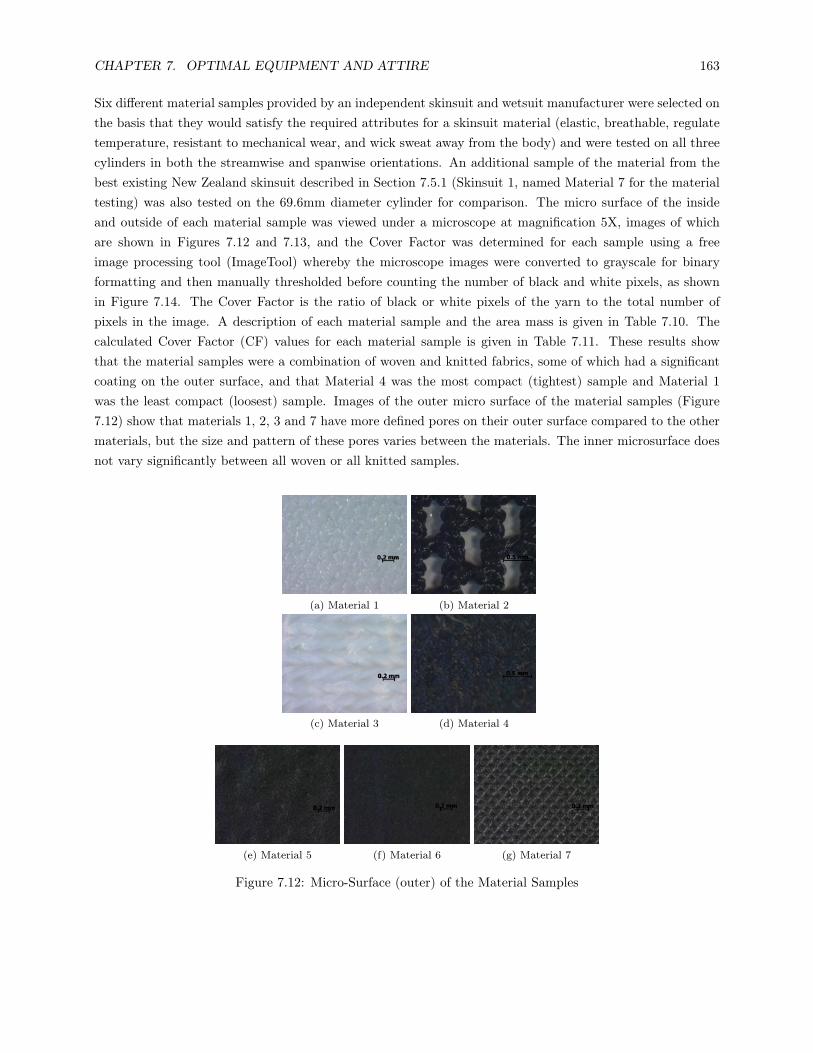
CHAPTER 7. OPTIMAL EQUIPMENT AND ATTIRE 163
Six di!erent material samples provided by an independent skinsuit and wetsuit manufacturer were selected onthe basis that they would satisfy the required attributes for a skinsuit material (elastic, breathable, regulatetemperature, resistant to mechanical wear, and wick sweat away from the body) and were tested on all threecylinders in both the streamwise and spanwise orientations. An additional sample of the material from thebest existing New Zealand skinsuit described in Section 7.5.1 (Skinsuit 1, named Material 7 for the materialtesting) was also tested on the 69.6mm diameter cylinder for comparison. The micro surface of the insideand outside of each material sample was viewed under a microscope at magnification 5X, images of whichare shown in Figures 7.12 and 7.13, and the Cover Factor was determined for each sample using a freeimage processing tool (ImageTool) whereby the microscope images were converted to grayscale for binaryformatting and then manually thresholded before counting the number of black and white pixels, as shownin Figure 7.14. The Cover Factor is the ratio of black or white pixels of the yarn to the total number ofpixels in the image. A description of each material sample and the area mass is given in Table 7.10. Thecalculated Cover Factor (CF) values for each material sample is given in Table 7.11. These results showthat the material samples were a combination of woven and knitted fabrics, some of which had a significantcoating on the outer surface, and that Material 4 was the most compact (tightest) sample and Material 1was the least compact (loosest) sample. Images of the outer micro surface of the material samples (Figure7.12) show that materials 1, 2, 3 and 7 have more defined pores on their outer surface compared to the othermaterials, but the size and pattern of these pores varies between the materials. The inner microsurface doesnot vary significantly between all woven or all knitted samples.
(a) Material 1 (b) Material 2
(c) Material 3 (d) Material 4
(e) Material 5 (f) Material 6 (g) Material 7
Figure 7.12: Micro-Surface (outer) of the Material Samples

CHAPTER 7. OPTIMAL EQUIPMENT AND ATTIRE 164
(a) Material 1 (b) Material 2
(c) Material 3 (d) Material 4
(e) Material 5 (f) Material 6 (g) Material 7
Figure 7.13: Micro-surface (inner) of the Material Samples
Figure 7.14: Calculating the Cover Factor using Image Processing

CHAPTER 7. OPTIMAL EQUIPMENT AND ATTIRE 165
Material Coating Area Mass (gm!2)
1 78% polyamide, 22% elastane, woven Lightweight polyurethane membrane 187
2 78% polyamide, 22% elastane, woven Polyurethane in ’honey-comb’ texture 293
3 80% polyamide, 20% elastane, knitted Dimpled polyurethane 213
4 80% polyamide, 20% elastane, knitted Dimpled polyurethane with 267
heavy all-over polyurethene induction
5 70% polyamide, 30% elastane, woven Waterproof membrane 213
6 76% polyamide, 24% polyeurothane elastane, knitted unknown coating 187
7 rubberised lycra with bonded seams, knitted unknown coating 213
Table 7.10: Properties of the Material Samples
Material # Black # White % Black % White Total # Cover Yarn Colour in ImagePixels Pixels Pixels Pixels Pixels Factor (Black or White)
1 726373 612627 54.25 45.75 1339000 0.46 White2 888515 450485 66.36 33.64 1339000 0.66 Black3 357050 981950 26.67 73.33 1339000 0.73 White4 1171141 167859 87.46 12.54 1339000 0.87 Black5 467845 871155 34.94 65.06 1339000 0.65 White6 529708 809292 39.56 60.44 1339000 0.60 White7 932651 406349 69.65 30.35 1339000 0.70 Black
Table 7.11: Calculated Cover Factor Values for all Material Samples
The thickness of each material sample was determined by placing each sample under the microscope at amagnification of 5X and measuring the height of the peaks and troughs, including the coating, as shown inFigure 7.15. The results are shown in Table 7.12, and clearly show that Material 5 is by far the thinnest(0.274mm), and Material 2 is the thickest (0.660mm); the thickness varied by only 0.386mm between samples.By placing the materials on the cylinders, the diameter of the cylinders would only increase by a minimumof 0.548mm and a maximum of 1.32mm. Figure 7.15 also clearly shows the di!erence in structure betweenthe woven and knitted fabrics, and between the di!erent coatings.
Material Thickness (±0.005mm)1 0.410mm2 0.660mm3 0.555mm4 0.630mm5 0.274mm6 0.480mm7 0.422mm
Table 7.12: Thickness of Material Samples

CHAPTER 7. OPTIMAL EQUIPMENT AND ATTIRE 166
(a) Material 1 (b) Material 2
(c) Material 3 (d) Material 4
(e) Material 5 (f) Material 6
(g) Material 7
Figure 7.15: Thickness of Materials

CHAPTER 7. OPTIMAL EQUIPMENT AND ATTIRE 167
The elastic modulus of the materials was determined by placing a 150mm by 25mm sample of each materialin an Instron machine (MTS 858 Desktop load frame with 10 kN load cell) and applying load to a maximumdisplacement of 95mm at a test speed of 300±10mm/min. In order to determine whether the orientation ofthe weave had any e!ect on the elasticity of the materials, samples of each material in the warp, weft and biasorientations were cut to size. Each material sample was then clamped in the instron machine at a pressure of15±2psi and stretched to maximum displacement or until failure. The clamped area of the material samplesand the area where direct extension occurred can be seen in Figure 7.16. Each material sample was onlystretched for one cycle, as during elite track cycling competitions athletes wear a new skinsuit when racing.Therefore it was deemed unneccesary to analyse the elastic properties of each material sample under cyclicloading, although it would be expected that there would be some loss in elastic modulus during repeat cycles.It was also expected that the materials would be strongest in the bias orientation, due to the no-slip condition.
Figure 7.16: Clamped Area and Area where Direct Extension Occurred for each Material Sample
The force-displacement and stress-strain curves were generated for each sample, and the force at maximumdisplacement (95mm displacement, 1.26 strain) or at failure was determined for each material. The stress-strain curves are shown in Figure 7.17, and a bar chat of the force at maximum displacement or at failurefor each sample shown in Figure 7.18.

CHAPTER 7. OPTIMAL EQUIPMENT AND ATTIRE 168
Figure 7.17: Stress-Strain Curve
Figure 7.18: Force at Maximum Displacement (95mm) or Failure
The results for the elasticity of the materials show that the relationship between stress and strain is almostlinear for most materials when stretched to maximum displacement. Only Material 2 in the weft orientation

CHAPTER 7. OPTIMAL EQUIPMENT AND ATTIRE 169
failed, at a stress of 11.64MPa and strain of 1.19, which suggests that all other samples are strong and havegood stretchability. All materials had a low stress up to 0.4 strain, with Material 5 showing a slightly higherstress up to 0.4 strain in all orientations compared to the other materials tested. At 0.4 strain Material 2 inthe warp orientation showed a large increase in stress. Materials 4 and 7 appeared to have the lowest force atmaximum deformation, suggesting these two materials were the most elastic out of all samples tested. Theresults show that all materials except for Material 2 in the weft orientation would be suitable for skinsuitmaterial, as no permanent deformation was observed, although materials 4 and 7 provide a more gentle andlinear stretching force. The results also show that the stress-strain curve did not di!er significantly for mostmaterials regardless of the orientation. This information is useful for the manufacturers of skinsuits, as theywould not need to take into account the orientation of the material when cutting the patterns for a skinsuitmade out of any of these materials, except perhaps for Material 2.
A calculation of the elastic modulus was performed for each material sample in all orientations to a strain of0.6. This strain value was chosen as it represented the actual strain of a skinsuit on a swimmer’s thigh [Searle,2012], which was thought to be similar to the actual strain of a skinsuit on a cyclist. In order to calculate theelastic modulus a second order polynomial trend line was fitted to the stress strain curve for each materialsample in each orientation up to a strain of 0.6, and the equation of the trend line di!erentiated. Thisdi!erential is equivalent to the elastic modulus, which was calculated for a strain of 0.6. The stress-straincurves and polynomial trends for each material sample are shown in Figure 7.19, and the calculated elasticmodulus for each sample in each orientation shown in Table 7.13.

CHAPTER 7. OPTIMAL EQUIPMENT AND ATTIRE 170
(a) Material 1 (b) Material 2
(c) Material 3 (d) Material 4
(e) Material 5 (f) Material 6
(g) Material 7
Figure 7.19: Stress-Strain Curves to 0.6 Strain and Polynomial Trend

CHAPTER 7. OPTIMAL EQUIPMENT AND ATTIRE 171
Material Orientation Elastic Modulus at 0.6 strain (MPa)Bias 1.00
Material 1 Warp 1.79Weft 2.22Bias 2.07
Material 2 Warp 2.63Weft 10.02Bias 0.65
Material 3 Warp 0.86Weft 0.55Bias 0.26
Material 4 Warp 0.05Weft 0.12Bias 1.14
Material 5 Warp 1.87Weft 3.30Bias 0.33
Material 6 Warp 0.41Weft 0.88Bias 0.18
Material 7 Warp 0.23Weft 0.14
Table 7.13: Elastic Modulus of each Material Sample in each Orientation
The results in Table 7.13 show that the elastic modulus for Material 2 is significantly greater in the weftorientation compared to the bias and warp orientations (a 74-79% increase in elastic modulus). Materials 1and 5 also showed a relatively large increase in elastic modulus in the weft orientation compared to the bias orwarp orientations, but for all other materials the elastic modulus did not di!er significantly with orientation.The orientation which resulted in the lowest elastic modulus di!ered between materials; the elastic moduluswas lowest in the bias orientation for Materials 1, 2, 5 and 6, the warp orientation for Material 4, and theweft orientation for Materials 3 and 7. The results also show that Materail 7 had a relatively low elasticmodulus in all orientations, which could have been due to the rubberised lycra material.
Although the results show that the stress-strain curves did not di!er significantly between the orientations,except for Material 2, it is possible that these materials will have di!erent aerodynamic properties dependingon the strain. Therefore the aerodynamic drag of all the materials in the warp orientation at 0.2 and 0.6 strainwas measured by placing sheaths on the 69.6mm diameter cylinder in the streamwise orientation with thesimple, stitched seam underneath, and placing the cylinder in the high speed wind tunnel at wind speeds of50kph, 60kph and 70kph. The drag of the supporting rods for the cylinder was subtracted from the measureddrag so that only the drag of the cylinder was used to calculate the drag coe"cient. The results are shownin Figure 7.20.

CHAPTER 7. OPTIMAL EQUIPMENT AND ATTIRE 172
Figure 7.20: Drag coe"cient for material samples at 0.2 and 0.6 strain on the 69.9mm diameter cylinder inthe streamwise orientation
It appears that only Material 7 shows a significant decrease in drag coe"cient with increase in strain, andthat for all other materials there are no consistent trends between the drag coe"cient at 0.2 and 0.6 strainoutside the error bars. These results suggest that the degree to which the material is stretched when on anathlete in their racing position would only be important if Material 7 was used as the material to make theskinsuit.
Another factor which must be considered when analysing di!erent materials for skinsuits is the surfaceroughness. The roughness of the material samples could not be analysed using the Talysurf 10 (TaylorHobson Inc.) because some samples were too rough to be detected. Therefore the thickness of the peaksand troughs of the samples were estimated using a microscope with a magnification factor of 5X to providea value for the depth, d, of the excrescences, as can be seen in Table Figure 7.21 and 7.14. In addition, theaverage length, L, and width, W, of the excrescences (average of 5 measurements at random locations) andthe distance between the centres of excrescences, A, were estimated for each material, as shown in Figure 7.22and Table 7.15. A roughness factor, k, and dimensionless roughness coe"cient, r, could then be calculatedusing Equations 7.1 and 7.2 respectively to provide a roughness scale for the samples [Oggiano et al., 2006],where r is the dimensionless roughness coe"cient, k is the roughness factor (mm), W is the width of theexcrescences (mm), d is the depth of the excrescences (mm), and D is the diameter of the cylinder (m). Theresults for the roughness factor and roughness coe"cient can be seen in Table 7.16. It was assumed that theheight of the coating for the coated materials was equal to the maximum depth of the protrusions, and thatthe coated materials were smoother than the uncoated materials, because the length, width and distancebetween excrescences could not be measured for the coated samples. The rank of the material samples fromrough to smooth can be seen in Table 7.17.

CHAPTER 7. OPTIMAL EQUIPMENT AND ATTIRE 173
k =#W.d (7.1)
r =k
D(7.2)
Figure 7.21: Depth of excrescences for Material 4
Material Peak Height Trough Height Height of Peaks Above Troughs Rank of Materials(mm) (mm) (Depth) (mm) Rough to Smooth
1 0.410mm 0.300mm 0.110mm Material 22 0.660mm 0.355mm 0.305mm Material 33 0.555mm 0.470mm 0.085mm Material 14 0.630mm 0.600mm 0.030mm Material 45 0.274mm 0.250mm 0.024mm Material 76 0.480mm 0.415mm 0.065mm Material 67 0.422mm 0.378mm 0.044mm Material 5
Table 7.14: Height of Peaks and Troughs of the Material Samples

CHAPTER 7. OPTIMAL EQUIPMENT AND ATTIRE 174
Figure 7.22: Calculating the length, L, and width, W, of excrescences and the distance, A, between them
Material Depth, d Width, W Length, L Distance, A k(µm) (µm) (µm) (µm) (µm)
1 110 203 220 234 1492 305 630 246 948 4383 85 642 573 1066 854 30 N/A N/A N/A N/A5 24 N/A N/A N/A N/A6 68 N/A N/A N/A N/A7 26 51 51 67 36
Table 7.15: Parameters of Material Samples
Material k r(mm) (D=56mm) (D=69.6mm) (D=111mm)
1 0.149 2.7x10!3 2.1x10!3 1.3x10!3
2 0.438 7.8x10!3 6.3x10!3 3.9x10!3
3 0.085 1.5x10!3 1.2x10!3 0.7x10!3
4 N/A N/A N/A N/A5 N/A N/A N/A N/A6 N/A N/A N/A N/A7 0.036 0.7x10!3 0.5x10!3 0.3x10!3
Table 7.16: Roughness Factor and Roughness Coe"cient of Material Samples

CHAPTER 7. OPTIMAL EQUIPMENT AND ATTIRE 175
Rank According to Peaks and Troughs According to Roughness FactorRoughest 2 2
| 3 3| 1 1| 4 7| 7
\|/ 6Smoothest 5
Table 7.17: Rank of Materials: Rough to Smooth
These results show that Material 2 was the roughest sample tested, and Materials 5, 6 and 7 were thesmoothest. The influence of surface roughness on circular cylinders in the spanwise orientation has beenanalysed by Hoerner [1965] who showed that the critical surface roughness is dependent on Reynolds number,and that the drag coe"cient can be reduced between 5x10⁴<Re<4x10⁵ by using varying degrees of surfaceroughness (Figure 7.23).
Figure 7.23: E!ect of surface roughness on drag coe"cient
Using the information from Figure 7.23 [Hoerner, 1965] it is possible to predict which material sample willhave the lowest drag coe"cient on each of the circular cylinders in the spanwise orientation. Firstly, theReynolds number for the circular cylinders in the spanwise orientation between 50kph and 80kph must becalculated (Table 7.18):
Speed (kph)Cylinder 49.5 53.8 57.6 61 64.3 71.5 78.8
Small (Ø=0.056m) 0.51 0.55 0.59 0.63 0.66 0.73 0.81Re (x105) Medium (Ø=0.0696m) 0.63 0.69 0.74 0.78 0.82 0.91 1.00
Large (Ø=0.111m) 1.01 1.09 1.17 1.24 1.31 1.45 1.60
Table 7.18: Reynolds Number for the Three Cylinders in the Spanwise Orientation

CHAPTER 7. OPTIMAL EQUIPMENT AND ATTIRE 176
It is then possible to determine the roughness coe"cient, k, that would result in the lowest drag coe"cientfor each cylinder at the relevant speeds. For example, the small cylinder, with a diameter of 0.056m, at 61kphhas a Reynolds number of 0.63x10⁵, which from Figure 7.23 shows that the lowest drag coe"cient occurs atkd = 2
102 = 0.02, so k=1.1mm. The calculated optimal roughness coe"cients for all cylinders at all speedsare shown in Table 7.19:
Speed (kph)Cylinder 49.5 53.8 57.6 61 64.3 71.5 78.8Small (Ø=0.056m) 1.1 1.1 1.1 1.1 1.1 0.5 0.4
k (mm) Medium (Ø=0.0696m) 1.4 1.4 0.6 0.6 0.5 0.3 0.1Large (Ø=0.111m) 0.4 0.4 0.4 0.4 0.4 0.4 0.2
Table 7.19: Optimal Surface Roughness for Cylinders in the Spanwise Orientation according to Hoerner[1965]
Tables 7.18 and 7.19 show that according to Hoerner [1965] the material samples should have a roughnessbetween k =0.1mm and 1.4mm, depending on the diameter of the cylinder and wind speed, in order to obtainthe lowest possible drag coe"cient. This would suggest that for wind speeds between 50kph and 80kph onlyMaterials 1 and 2 are rough enough to cause the drag coe"cient to drop when on the circular cylinders in thespanwise orientation. As the materials are stretched over the circular cylinders it would be expected that theroughess coe"cient would be reduced slightly. However, the results for the aerodynamic drag when stretched(Figure 7.20) suggests that there is no significant change to the surface roughness for the degree to which thematerials are stretched over the cylinders, as there was no significant gain or loss in drag coe"cient for therougher materials (Material 2).
7.5.2.3 Aerodynamic Drag of Material Samples
Once the thickness, elasticity, and roughness of all the material samples had been analysed it was possibleto compare the aerodynamic drag of all the materials in both the streamwise and spanwise orientations. Allmaterial samples were stretched to 0.6 strain and cut in the bias orientation, as all material samples showeda relatively low elastic modulus in this orientation, and the material would remain in the bias orientationwhen on both the streamwise and spanwise cylinders.
Streamwise Orientation: seam underneath cylinder
The drag coe"cient was calculated for each material sample when placed on each cylinder in the streamwiseorientation, and the results plotted against the Reynolds number, as shown in Figure 7.24.

CHAPTER 7. OPTIMAL EQUIPMENT AND ATTIRE 177
(a) Small Cylinder (56mm diameter) (b) Medium Cylinder (69.6mm diameter)
(c) Large Cylinder (110mm diameter cylinder)
Figure 7.24: Drag coe"cient against Reynolds number for the circular cylinders in the streamwise orientationwith the seam underneath
The results in Figure 7.24 show that there is virtually no di!erence in the drag coe"cient for the di!erentmaterials on the medium and large cylinders, but on the small cylinder Materials 5 and 6 appeared to havea lower drag coe"cient than Materials 2 and 4 in particular. No material showed a significant drop in dragcoe"cient within the range of Reynolds numbers tested, which was as expected as there is no drag crisisat these Reynolds numbers for this particular geometry. It is possible that base drag, on which noise issuperimposed, dominates all other e!ects on the cylinders in the streamwise orientation, which would explainthe similar drag coe"cient values between di!erent material samples on all cylinders tested.
According to Hoerner [1965] the drag coe"cient for circular cylinders in axial flow is dependent on the lengthto diameter ratio, L/D, and at L/D=0.5 a significant reduction in drag coe"cient is seen, Figure 7.25. Thelength to diameter ratios for the small, medium and large cylinders are 2.68, 2.16 and 1.35 respectively,which is significantly higher than the length to diameter ratio for which a reduction in drag coe"cient wouldbe expected from Figure 7.25. The actual drag coe"cient values for the small, medium and large cylindershowever, are within the same range as the drag coe"cient values reported by Hoerner [1965] for circular

CHAPTER 7. OPTIMAL EQUIPMENT AND ATTIRE 178
cylinders in axial flow with similar length to diameter ratios (represented by the red markers on Figure 7.25).
Figure 7.25: Comparison between drag coe"cient results for cylinders and the results by Hoerner [1965]
A comparison of the Reynolds number of the streamwise parts of the body of a cyclist (forearm) to theReynolds number of the cylinders in the streamwise orientation will enable the material with the lowest dragto be identified, as shown in Table 7.20. These results show that Material 5, one of the smoothest materials,appears to have a consistently low, although not necessarily always the lowest, drag coe"cient for parts ofthe body in the streamwise orientation (forearms) at cycling speeds between 40kph and 70kph. Material 5would therefore be the best choice of material to use for these parts of the body at speeds between 40 and70kph. These results agree with Brownlie et al. [2009] who also found that smooth materials had a lowerdrag on streamwise parts of the body as they provided the least frictional drag.
Cycling Speed (kph) Recyclist (x105) Corresponding Cylinder Material with the Lowest Cd
40 2.7 Small 64kph 5 or 650 3.4 Medium 71kph 1, 5 or 760 4.1 Large 65kph Any70 4.7 Large 76kph Any
Table 7.20: Optimal material for the forearm of a cyclist
Spanwise Orientation: seam behind cylinder
The drag coe"cient was calculated for each material sample when placed on each cylinder in the spanwiseorientation, and the results plotted against the Reynolds number (Figure 7.26).
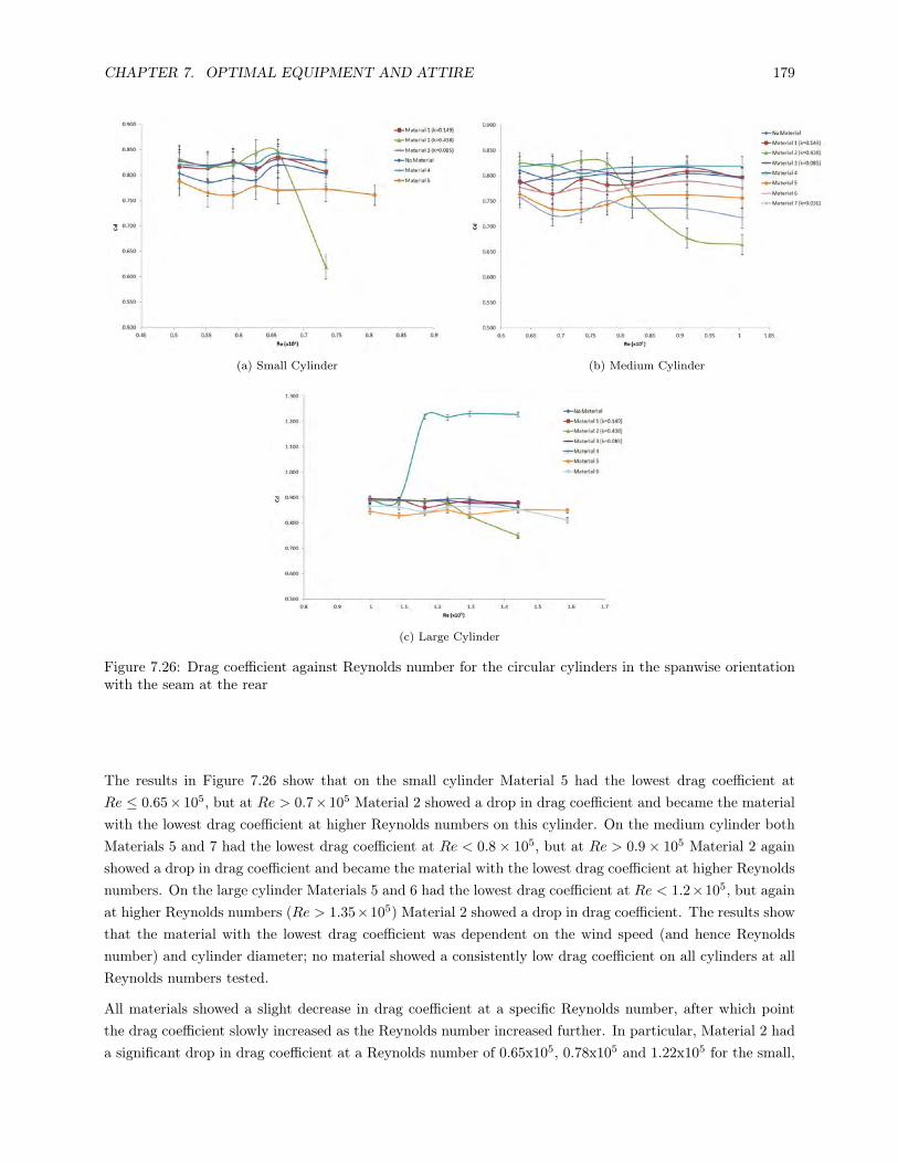
CHAPTER 7. OPTIMAL EQUIPMENT AND ATTIRE 179
(a) Small Cylinder (b) Medium Cylinder
(c) Large Cylinder
Figure 7.26: Drag coe"cient against Reynolds number for the circular cylinders in the spanwise orientationwith the seam at the rear
The results in Figure 7.26 show that on the small cylinder Material 5 had the lowest drag coe"cient atRe & 0.65" 105, but at Re > 0.7" 105 Material 2 showed a drop in drag coe"cient and became the materialwith the lowest drag coe"cient at higher Reynolds numbers on this cylinder. On the medium cylinder bothMaterials 5 and 7 had the lowest drag coe"cient at Re < 0.8" 105, but at Re > 0.9" 105 Material 2 againshowed a drop in drag coe"cient and became the material with the lowest drag coe"cient at higher Reynoldsnumbers. On the large cylinder Materials 5 and 6 had the lowest drag coe"cient at Re < 1.2"105, but againat higher Reynolds numbers (Re > 1.35"105) Material 2 showed a drop in drag coe"cient. The results showthat the material with the lowest drag coe"cient was dependent on the wind speed (and hence Reynoldsnumber) and cylinder diameter; no material showed a consistently low drag coe"cient on all cylinders at allReynolds numbers tested.
All materials showed a slight decrease in drag coe"cient at a specific Reynolds number, after which pointthe drag coe"cient slowly increased as the Reynolds number increased further. In particular, Material 2 hada significant drop in drag coe"cient at a Reynolds number of 0.65x10⁵, 0.78x10⁵ and 1.22x10⁵ for the small,

CHAPTER 7. OPTIMAL EQUIPMENT AND ATTIRE 180
medium and large cylinders respectively, which corresponds to the critical Reynolds number region for roughcylinders in axial flow (6.4x10⁴ < Re <1.4x10⁵). This trend is typical for rough cylinders in axial flow, aswas shown in Figure 7.23, where the reduction in drag coe"cient and the Reynolds number at which thisdrop in drag coe"cient takes place is dependent on the surface roughness and diameter of the cylinder, afterwhich point the drag coe"cient begins to increase again due to an increase in surface friction.
It was expected that only Materials 1 and 2 would be rough enough to cause the drag coe"cient to drop whenon the circular cylinders in the spanwise orientation, but the results in Figure 7.26 suggest that only Material2 was actually rough enough to trip the boundary layer from laminar to turbulent flow. The reduction in dragceo"cient for Material 2 on the three cylinders in axial flow was slightly lower than the empircal reductionin drag coe"cient for similar roughness coe"cients to diameter ratios shown in Figure 7.23 [Hoerner, 1965].This discrepancy is most likely due to the fact that the cylinders used for this study had rounded ends ratherthan blunt ends, and the materials also had a seam which may have a!ected the flow. As Material 2 failed inthe weft orientation it would be unwise to make a skinsuit out of Material 2 cut in this orientation. However,cutting Material 2 in the bias orientation would be suitable and would also provide the lowest drag coe"cientat higher Reynolds numbers. Material 4 showed an unexpected increase in drag coe"cient with Reynoldsnumber on the large cylinder, which could be due to delamination of the coating on Material 4 when it wasstretched over the cylinder.
A comparison of the Reynolds number of the spanwise parts of the body of a cyclist (upper arms and thighs) tothe Reynolds number of the cylinders in the spanwise orientation will enable the most aerodynamic materialto be identified, as shown in Table 7.21 (where the seam is located at the rear of the cylinder for all cases).These results show that a smooth material (Material 5, 6 or 7) is optimal for the forearms, as the Reynoldsnumber has not yet reached the point at which turbulence should be induced, but for the thighs at cyclingspeeds (50kph the roughness of Material 2 trips the flow from laminar to turbulent and reduces the dragcoe"cient. As most elite cyclists spend the majority of their race at speeds greater than 50kph it wouldrecommended for the thighs to be made out of Material 2.
Cycling Speed (kph) Recyclist (x105) Corresponding Cylinder Tested Most Aerodynamic Material
40 0.66 Medium 49.5kph (Re=0.63x10⁵) 5 or 7Upper Arm 50 0.82 Medium 64.3kph (Re=0.82x10⁵) 5 or 7
60 0.99 Large 49.5kph (Re=1.00x10⁵) 5 or 670 1.15 Large 57.6kph (Re=1.15x10⁵) 5 or 640 1.17 Large 57.6kph (Re=1.15x10⁵) 5 or 6
Thigh 50 1.47 Large 71.5kph (Re=1.44x10⁵) 260 1.76 Large 78.8kph (Re=1.59x10⁵) Not tested - 2?70 2.05 Large 102kph Not tested - 2?
Table 7.21: Optimal material for the upper arms and thighs of a cyclist
Spanwise Orientation: comparison of seam placement
As previous studies have shown that trips are a successful method of reducing the drag coe"cient as well assurface roughness (see Section 3.2.1.4) it was necessary to analyse the e!ect of the seam placement as wellas material roughness on the drag coe"cient. A comparison of seam placement was made by measuring the

CHAPTER 7. OPTIMAL EQUIPMENT AND ATTIRE 181
drag of each material on the medium and large cylinders in the spanwise orientation and rotating the seamfrom 0° (stagnation point) to 180° (rear) in 30° increments. Plots of the drag coe"cient against Reynoldsnumber were made for each material to compare the seam placement, as shown in Figure 7.27.
(a) Material 1 (b) Material 2
(c) Material 3 (d) Material 4
(e) Material 5 (f) Material 6
Figure 7.27: Comparison of seam placement for each material on the medium spanwise cylinder

CHAPTER 7. OPTIMAL EQUIPMENT AND ATTIRE 182
(a) Material 1 (b) Material 2
(c) Material 3 (d) Material 5
(e) Material 6
Figure 7.28: Comparison of seam placement for each material on the large spanwise cylinder*

CHAPTER 7. OPTIMAL EQUIPMENT AND ATTIRE 183
* The coating of the sheath of Material 4 for the large cylinder began to peel away from the surface, so wasnot tested.
The results in Figures 7.27 and 7.28 show that the drag coe"cient varies for each material depending on theReynolds number and seam placement. Material 2 was the only material that showed a significant drop indrag coe"cient, although this drop in drag coe"cient occured at di!erent Reynolds numbers depending onthe placement of the seam. By placing the seam at 60° on the large cylinder the drag coe"cient was reducedfor all materials at all Reynolds numbers tested, with the exception of Material 2 which showed a drop indrag coe"cient at a di!erent Reynolds number depending on the seam placement. However, a di!erent trendwas seen on the medium cylinder where the drag coe"cient was higher for Materials 1 and 6 with the seamat 60°, but significantly lower for Materials 4 and 5 with the seam at 60°. Again Material 2 showed a drop indrag coe"cient at a di!erent Reynolds number depending on the seam placement on the medium cylinder.These results highlight the importance of selecting the material and seam placement depending on the speedof the cyclist and the size of the upper arm and thigh. It should be noted that the seam was formed in thesame way for all material samples, created by sewing a simple stitch to join the material when inside-out,and then turning the material sample the right-way so that the two un-joined ends were sitting on the insideof they cylinder, as shown in Figure 7.29.
Figure 7.29: Simple, stitched seam
In order to identify the optimal material and seam placement for the body parts of a cyclist in the spanwiseorientation it is necessary to compare the Reynolds number of the upper arm and thigh to the Reynoldsnumber of the cylinders in the spanwise orientation, as shown in Figure 7.30 and Table 7.22. By analysingboth the material and seam placement the best possible combination in terms of aerodynamic drag can bedetermined.

CHAPTER 7. OPTIMAL EQUIPMENT AND ATTIRE 184
(a) Re=0.63x10⁵ (b) Re=0.82x10⁵
(c) Re=1x10⁵ (d) Re=1.15x10⁵
(e) Re=1.44x10⁵ (f) Re=1.59x10⁵
Figure 7.30: Comparison of material and seam placement for the Reynolds number of the upper arm andthigh of a cyclist

CHAPTER 7. OPTIMAL EQUIPMENT AND ATTIRE 185
Cycling Speed(kph)
Recyclist
(x105)Corresponding Cylinder Tested Most Aerodynamic Material
40 0.66 Medium 49.5kph (Re=0.63x10⁵) 4 or 5 seam 60°
Upper Arm 50 0.82 Medium 64.3kph (Re=0.82x10⁵) 4 or 5 seam 60°, or 2 seam 30°
60 0.99 Medium 78.8kph (Re=1.00x10⁵) 2 seam any location except 120°, or 4 or 5 seam 60°
70 1.15 Large 57.6kph (Re=1.15x10⁵) 1, 3, 5 or 6 seam 60°
40 1.17 Large 57.6kph (Re=1.15x10⁵) 1, 3, 5 or 6 seam 60°
Thigh 50 1.47 Large 71.5kph (Re=1.44x10⁵) 2 seam 0°, 30°, 150° or 180°
60 1.76 Large 78.8kph (Re=1.59x10⁵) 2 seam 0°, 30°, 150° or 180°
70 2.05 Large 102kph not tested (2 seam 0°, 30°, 150° or 180°?)
Table 7.22: Optimal material for the upper arm and thigh of a cyclist
The results in Table 7.22 show that the lowest drag coe"cient does not necessarily occur with a smoothmaterial, as was found when the seam location was not taken into account. The optimal material and seamplacement when the location of the seam is considered is dependent on the cylinder size and wind speed. Atlower Reynolds numbers (Re & 0.63"105) a smoother material (Material 4 or 5) with the seam at 60° had thelowest drag coe"cient. As the Reynolds number increased (0.63"105 < Re < 1.15"105), although smoothermaterials (Material 4 or 5) with the seam at 60° still had a low drag coe"cient, rougher materials (Material2) showed a drop in drag coe"cient when the seam was is in a specific location, resulting in a similar valueof drag coe"cient to the smoother materials. At Re = 1.15 " 105 all materials except for Material 2 (theroughest material) had a low drag coe"cient when the seam was at 60°, but a further increase in Reynoldsnumber (Re > 1.15"105) resulted in the roughest material (Material 2) having the lowest drag coe"cient at0°, 30°, 150° or 180°. Therefore, these results highlight the importantance of determining the average speedof each individual cyclist before selecting the material and seam placement for a skinsuit design.
The primary objective for analysing materials and seam placement for cycling skinsuits was to develop a newskinsuit design for endurance track cyclists, whose cycling speed tends to be relatively constant at 53kph forfemale athletes and 56kph for male athletes. Considering the fact that the coating on Material 4 showed signsof delamination, it would be recommended to use Material 5 with the seam at 60° for the upper arms, andto use Material 2 with the seam at 0°, 30°, 150° or 180° for the thighs. The selection of the seam placementof Material 2 on the thighs could therefore be dependent on ease of manufacture of the skinsuit.
By comparing the roughness coe"cient with the minimum drag coe"cient for the materials on the cylindersin the spanwise orientation, Figure 7.31, it is clear to see that the aerodynamic drag can be reduced bymanipulating both the surface roughness and seam placement. Figure 7.31 shows that an increase in surfaceroughness reduces the drag coe"cient for when the seam is both at the rear of the cylinder and when inthe most aerodynamic position. This suggests that surface roughness is more significant at reducing theaerodynamic drag than using a seam to trip the flow, but an analysis of both material roughness and seamplacement will provide the best results.

CHAPTER 7. OPTIMAL EQUIPMENT AND ATTIRE 186
Figure 7.31: Relationship between the roughness coe"cient on Cdmin
The influence of the cylinder diameter on the aerodynamic properties of the cylinder can be determined bycomparing the relationship between the diameter of the cylinders and the minimum value of drag coe"cient,Cdmin, when the seam for each material was placed at the rear of the cylinder (180°) and in the locationyielding the lowest drag. This relationship is shown in Figure 7.32, which highlights that in general anincrease in diameter causes an increase in the minimum drag coe"cient, with the exception of most materialson the small cylinder. It is possible that the ratio of the seam size relative to the cylinder diameter has somea!ect on the drag coe"cient, which must also be taken into account, and this could be a possible explanationfor the higher Cdmin values observed on the small cylinder compared to the medium cylinder.

CHAPTER 7. OPTIMAL EQUIPMENT AND ATTIRE 187
Figure 7.32: Relationship between Cdmin and the cylinder diameter
These results from these studies on material roughness, seam location and cylinder diameter have shown thatthe roughness of the fabric, the diameter of the cylinder, and also the location and size of the seam relativeto the diameter of the cylinder all have an influence on the aerodynamic properties of the cylinder.
7.5.2.4 Most Significant Factor on Aerodynamic Drag
In order to determine the most significant factor on the drag coe"cient for di!erent parts of the body atracing speeds the greatest di!erence in drag coe"cient was determined for each material factor at 50kph and60kph, as shown in Tables 7.23 and 7.24 respectively. The results indicate that the type of material usedhas the most influence on the aerodynamic drag for parts of the body in the streamwise orientation, but inthe spanwise orientation the seam placement or the material type both have a significant influence on dragcompared to all other factors.

CHAPTER 7. OPTIMAL EQUIPMENT AND ATTIRE 188
!Cd Forearm !Cd Upper Arm !Cd ThighMedium Cylinder 71kph Medium Cylinder 64.3kph Large Cylinder 71.5kph
Factor Re=3.4x10⁵ Re=0.82x10⁵ Re=1.5x10⁵
Roughness 0.038 0.056 0.093Thickness 0.038 0.056 0.093Material 0.045 0.059 0.125Stretch 0.038 n/a n/a
Seam placement n/a 0.150 0.081Knit vs weave 0.045 0.059 0.125
Maximum Di!erence in Cd 0.045 0.150 0.125Most Significant Factor Material Seam Placement Material
Table 7.23: Most significant factors for parts of the body for cycling at 50kph
!Cd Forearm !Cd Upper Arm !Cd ThighLarge Cylinder 65kph Medium Cylinder 78.8kph Large Cylinder 78.8kph
Factor Re=4.1x10⁵ Re=0.99x10⁵ Re=1.76x10⁵
Roughness 0.008 0.076 0.097Thickness 0.008 0.076 0.097Material 0.019 0.134 0.109Stretch not tested on large cylinder n/a n/a
Seam placement n/a 0.190 0.110Knit vs weave 0.019 0.134 0.109
Maximum Di!erence in Cd 0.019 0.190 0.110Most Significant Factor Material Seam Placement Seam Placement
Table 7.24: Most significant factors for parts of the body for cycling at 60kph
7.5.2.5 Summary
The results from analysing material type, seam location, cycling speed, cylinder diameter and cylinder ori-entation have identified the best possible material and seam placement for di!erent parts of the body fortrack cyclists, particularly for endurance athletes. The results have shown that for parts of the body in thestreamwise orientation (forearms) a smooth material is the best in terms of aerodynamics at 50-60kph, whichwas Material 5 for this study. For parts of the body in the spanwise orientation (upper arms and thighs) thebest material and seam placement in terms of aerodynamics was dependent on both the cycling speed andcylinder diameter. It was found that Material 5 with the seam at 60° would be the best combination for theupper arms at 50kph-60kph, and Material 2 with the seam at 0°, 30°, 150° or 180° would be the best combi-nation for the thighs at 50-60kph. The results from the stress-strain analysis showed that Material 2 failedin the weft orientation, so it would be unwise to use this material in this orientation for a skinsuit. However,in the bias or warp orientations Material 2 did not fail up to maximum load (95mm) and would thereforebe suitable as a skinsuit material. Material 5 did not fail to maximum load in any orientation and showeda relatively low elastic modulus, suggesting the orientation of the weave was not important for Material 5.

CHAPTER 7. OPTIMAL EQUIPMENT AND ATTIRE 189
However, when in the bias orientation Material 5 showed more gentle and linear stretching force compared tothe warp or weft orientations, which would be beneficial for cyclists when putting on the skinsuit. Material2 showed a slight increase in drag coe"cient with increase in strain, where as Material 5 showed a slightdecrease in drag coe"cient with strain at 50-70kph. This suggests that Material 2 should not be stretchedabove a strain of 0.2, where as Material 5 should be at a strain of 0.6 when the cyclist is in their racingposition.
7.5.2.6 Prototype Testing
Once an analysis had been carried out on di!erent materials and seam locations, a prototype skinsuit wasmade using the results from the circular cylinder tests. Although Material 2 was identified as a materialthat would provide a lower aerodynamic drag on the thighs, it was not possible to get hold of enough ofthis material within the required time frame, and the elastic modulus of this material was relatively highcompared to the other material samples. Therefore a decision was made to use only Material 5 to createa prototype skinsuit, as this material had been identified as being the best in terms of aerodynamics forthe forearms and upper arms, and was the second best in terms of aerodynamics for the thighs at speedsbetween 50 and 60kph. The results from the circular cylinder tests showed that for Material 5 the best seamplacement in terms of aerodynamics on the upper arms and thighs was at 60°. Therefore the skinsuit patternwas designed so that the seams would lie in this location when the athlete was in their racing position. Theseams for the forearms were designed to be underneath the forearms when the athlete was in their racingposition, and all other seams were designed for ease of manufacture of the skinsuit. The prototypes did notinclude a chamois during this early stage of development.
The prototype was made to fit a specific athlete so that it was tight fitting, and was compared to the mostaerodynamic, existing New Zealand skinsuit (Skinsuit 1 in Section 7.5.1, made from Material 7) to determinewhether the aerodynamic drag had been reduced through the new skinsuit design and choice of material.The athlete for which the prototype skinsuit was made for tested both skinsuits in the boundary layer windtunnel at 45kph, using their own equipment and adopting their current racing position, which was monitoredfrom side on by projecting their shadow on to the white board. The athlete was pedalling at 90rpm for alltests. The drag was measured three times consecutively for each skinsuit, as well as once for removing andputting back on each skinsuit to determine the repeatability of putting the skinsuit back on in the sameplace. Images of both the prototype and best existing New Zealand skinsuit (Skinsuit 1) on the athlete canbe seen in Figure 7.33 and the results for the measured aerodynamic drag are shown in Table 7.25.

CHAPTER 7. OPTIMAL EQUIPMENT AND ATTIRE 190
(a) Prototype Skinsuit (Material 5) (b) Existing New Zealand Skinsuit (Material 7)
Figure 7.33: Prototype Skinsuit Testing
Test # Prototype Skinsuit (Material 5) Existing NZ Skinsuit (Material 7)1 2.104 kg 2.108 kg2 2.102 kg 2.110 kg3 2.106 kg 2.111 kg
Average 2.104 kg 2.110 kgRepeat once removed 2.109 kg 2.107 kg
Repeatability 0.005 kg (0.24%) 0.003 kg (0.14%)
Table 7.25: Drag Results of Prototype Skinsuit Testing
The results in Table 7.25 show that the di!erence in measured aerodynamic drag between the two skinsuitswas only 0.006kg (0.28%), which is less than the 1% calculated repeatability of the cycle rig. These resultssuggest that although significant di!erences in drag were identified between Material 5 and Material 7 onthe circular cylinder models, especially in the spanwise orientation, the gains were not nearly as great whentransferred to a complete skinsuit. This could be due to the influence of the cycling equipment, the di!erencein seam type between the skinsuits, the moving legs of the athlete, and because the flow further downstream(towards the thighs) would be a!ected by the flow further upstream, which was not taken into account onthe cylinder models. Nevertheless, the initial prototype skinsuit has shown the potential for skinsuit design,and to be able to create an initial prototype that has the same aerodynamic drag as the best existing NewZealand skinsuit, which can now only be improved on, is a significant first step. Further development of theprototype skinsuit would include getting hold of Material 2 to use on the thighs, looking into di!erent typesof seams to identify the significance of bonded or raised seams on di!erent parts of the body, and to developthe design around the torso in a similar way to the circular cylinder body parts.

CHAPTER 7. OPTIMAL EQUIPMENT AND ATTIRE 191
7.6 Shoe Covers
In order to determine the influence of shoe covers on the aerodynamics of cyclists, wind tunnel tests werecarried out on an athlete in the boundary layer wind tunnel and also on a leg model in the high speed windtunnel. It was believed that the di!erence in drag between di!erent types of shoe covers would be small, andthat greater di!erences would be seen on a leg model compared to an athlete due to the greater contributionof the shoe cover to the overall drag on the leg model.
7.6.1 Athlete Tests
A male, elite track cyclist was used as the subject for analysing the influence of shoe covers on the aerodynamicdrag of a cyclist. Both stationary and pedalling tests were carried out, with the drag readings being accurateto ±1% (as calculated in Section 5.1.2.3). The cyclist used their own equipment and adopted their currentracing position for all tests. The cyclist wore Sidi Hi-Tech bike shoes with Shimano SPD SL cleats andpedals, but no socks were worn as this represented actual race conditions. The athlete pedalled at 90rpm forall dynamic tests, and maintained the same foot position for all stationary tests with the right foot at 270°and the left foot at 90° from the TDC (a horizontal foot position). In order to ensure the athlete maintainedthe same position for each test the shadow of the athlete from side on was projected onto a white boardand the shadow drawn around, and a camera was placed to the side of the athlete so that photos could becompared between tests. The frontal area of the athlete was calculated using the digitising method, and theambient temperature and pressure recorded for each test. A comparison was made between three di!erentshoe covers, as well as when no shoe cover was worn. Details of the shoe covers can be seen in Table 7.26 andFigure 7.34. The wind speed was set at 45kph and the aerodynamic drag measured. All tests were repeatedand the average drag was recorded.
Shoe Cover DescriptionPrototype 1 78%PES / 22% elastane, seam down front-middle,
zip at rear, one hole for cleat, 250mm highPrototype 2 78%PES / 22% elastane, seam around ankle,
zip at rear, one hole for cleat, 250mm highChampion Systems 80%PES / 20% elastane, seam down front-middle,
zip at rear, two holes for cleat, 200mm high
Table 7.26: Shoe Covers

CHAPTER 7. OPTIMAL EQUIPMENT AND ATTIRE 192
(a) Prototype 1 (b) Prototype 2
(c) Champion Systems
Figure 7.34: Shoe Covers used for Athlete Testing
The results of the measured aerodynamic drag for stationary and pedalling tests for all shoe covers and forthe shoe without any cover are shown in Figure 7.35.

CHAPTER 7. OPTIMAL EQUIPMENT AND ATTIRE 193
Figure 7.35: Drag results of shoe cover testing on an athlete
The results in Figure 7.35 show that a similar trend was observed for the stationary and pedalling tests, witha lower drag measured for all tests where a shoe cover was worn compared to no shoe cover. The Prototype 1shoe cover had the lowest drag, with a 2.5% reduction in drag compared to no shoe cover for pedalling tests.Both the Prototype 1 and Prototype 2 shoe covers were higher on the leg than the Champion System shoecovers (250mm compared to 200mm in height) and the aerodynamic drag was lower for these shoe covers.This suggests that the material used for shoe covers has a lower skin friction or lower pressure drag thanhuman skin, and that it is more beneficial to cover as much of the skin as possible in order to minimise thedrag of a cyclist. It should be noted that the UCI states that shoe covers must not exceed the mid-distancebetween the ankle and the knee [Reid, 2012]. The Prototype 1 and Champion Systems shoe covers both hada seam down the front-middle of the shoe cover, but the e!ect of the seam on the drag did not appear tobe as significant as the height of the shoe covers; the Prototype 1 shoe covers had the lowest drag and theChampion Systems shoe covers had the highest drag. However, a comparison between the Prototype 1 andPrototype 2 shoe covers suggests that it is more aerodynamic to have the seam down the front of the shoecover than across the ankle, probably because the seam down the front runs with the airflow, where as theseam around the ankle runs across the flow; the seam position was the only di!erence between the Prototype1 and Prototype 2 shoe covers, with the seam down the front on Prototype 1 and the seam across the ankleon Prototype 2 (Figure 7.36) and the Prototype 1 shoe covers had a lower drag.

CHAPTER 7. OPTIMAL EQUIPMENT AND ATTIRE 194
(a) Prototype 1: Seam downthe front
(b) Prototype 2: Seam acrossankle
Figure 7.36: Seam Placement Comparison
7.6.2 Leg Model Tests
A prosthetic lower leg used for paralympic road cycling was used to measure the aerodynamic drag of di!erentshoe covers and no shoe cover in the closed-section, high speed wind tunnel. The same shoe, cleat and pedalas used for the athlete tests (Sidi Hi-Tech shoe and Shimano SPD SL cleat and pedal) were used for the legmodel tests, but no crank was used. The maximum extended distance of the pedal and cleat from the sole ofthe shoe was 37.5mm. Tests were also carried out with shoe covers on the leg model with the cleat and pedalremoved to identify their influence on the aerodynamic drag. The lower leg was attached to a rod, which waspassed through the wind tunnel floor and then connected to a load cell so that the aerodynamic drag couldbe measured. The leg was placed upside down in the wind tunnel, with the shoe towards the ceiling, so thatthe shoe covers could be taken o! and put on easily without the need to dismantle the leg after each test.The set up is shown in Figure 7.37.

CHAPTER 7. OPTIMAL EQUIPMENT AND ATTIRE 195
Figure 7.37: Set up of Lower Leg Model in the High Speed Wind Tunnel
The aerodynamic drag was measured for the leg and shoe without a shoe cover on, as well as for six di!erentshoe covers, details of which are shown in Table 7.27 and Figure 7.38. The wind speed was varied from 50kphto 75kph to analyse the e!ect of speed on the aerodynamic drag of the shoe covers. Once all measurementshad been recorded, the tests were repeated a further three times for one shoe cover, each time fitting and thenremoving the shoe cover, to identify the repeatabilty of taking the shoe covers on and o!. The results werefound to be repeatable to ±3%. The frontal areas of (a) the shoe, (b) shoe and shoe cover, (c) the shoe, cleatand pedal, and (d) the shoe, cleat, pedal and shoe cover, were all calculated using the digitising method. Theerror associated with calculating the frontal area was determined by using the digitizing method to calculatethe frontal area of the shoe from the same image three times. The maximum di!erence in the frontal areacalculation was ±0.005m2.
Shoe Cover DescriptionPrototype 1 78% polyamid / 22% elastane, seam down front-middle,
zip at rear, one hole for cleat 250mm highPrototype 2 78% polyamid / 22% elastane, seam around ankle,
zip at rear, one hole for cleat 250mm highChampion Systems 80% polyamid / 20% elastane, seam down front-middle,
zip at rear, two holes for cleat, 200mm highBase 84% polyamid / 16% elastane, seam down front-middle,
no zip, two holes for cleat, 180mm highNike 80% polyamid / 20% elastane, coated, seam down front-middle,
zip at rear, two holes for cleat, 200mm highPearl Izumi 80% polyamid / 20% elastane, coated, seam down front-middle,
zip at rear, one hole for cleat, 180mm high
Table 7.27: Description of Shoe Covers

CHAPTER 7. OPTIMAL EQUIPMENT AND ATTIRE 196
(a) Prototype 1 (b) Prototype 2 (c) Champion Systems
(d) Base (e) Nike (f) Pearl Izumi
Figure 7.38: Shoe Covers used for Leg Model Testing
The measured drag results for the leg model tests without and with the cleat and pedal are shown in Figures7.39 and 7.40 respectively. The results show that there was a greater di!erence in drag between the shoecovers at faster wind speeds for tests both with and without the cleat and pedal. However, the trend betweenthe most and least aerodynamic shoe cover di!ered between the results without the cleat and pedal comparedto the results with the cleat and pedal. For example, the Base shoe cover was significantly less aerodynamicthan all other shoe covers when there was no cleat or pedal, but when a cleat and pedal were attached to theshoe the Base shoe cover was more aerodynamic than the Prototype 2 and Champion Systems shoe covers.This suggests that the cleat and pedal influence the flow around the shoe and should therefore be presentwhen analysing the aerodynamic drag of shoe covers in order to represent racing conditions more accurately.For this reason, only the results for the shoe covers with the cleat and pedal will be discussed further.

CHAPTER 7. OPTIMAL EQUIPMENT AND ATTIRE 197
Figure 7.39: Drag Results without the Cleat and Pedal
Figure 7.40: Drag Results with the Cleat and Pedal
For tests carried out with the cleat and pedal, the only significant di!erence identified was that the PearlIzumi shoe covers appeared to have a slightly lower drag compared to no shoe cover at all speeds tested;

CHAPTER 7. OPTIMAL EQUIPMENT AND ATTIRE 198
any other shoe cover showed a similar drag to no shoe cover at all speeds tested when a cleat and pedalwere present. Unlike the results in Section 7.6.1 for athlete tests where the Prototype 1, Prototype 2 andChampion Systems shoe covers had a lower drag compared to no shoe cover, these shoe covers all had asimilar or greater drag compared to no shoe cover when on the leg model. This suggests that the artificialleg has a lower drag compared to human skin.
The percentage reduction in drag for all shoe covers compared to no shoe cover for the tests on the leg modelwith the cleat and pedal are shown in Figure 7.41. The dotted lines represent the ±3% repeatability ofthe drag measurements, and a positive percentage relates to a reduction in drag and a negative percentagerelates to a gain in drag. These results show that although some shoe covers did reduce the drag at certainspeeds, only the Pearl Izumi shoe covers reduced the aerodynamic drag by more than the 3% repeatability atall speeds tested. The Champion Systems and Prototype 2 shoe covers appear to be the least aerodynamic,showing either a minimal reduction in drag or an increase in drag compared to no shoe covers.
Figure 7.41: Percentage Reduction in Drag for all Shoe Covers Compared to No Shoe Cover
The presence of a zip at the rear of the shoe covers did not appear to a!ect the aerodynamic drag, as theaerodynamic drag of the Base shoe cover (no zip) was neither significantly lower nor higher than the othershoe covers, all of which had a zip down the back. If the zip had been placed directly in the flow ratherthan at the rear of the shoe cover, out of the flow, it is likely that an increase in drag would have been seen.The number of holes for the cleat did not appear to influence the drag results either, as the Prototype 1,Prototype 2 and Pearl Izumi shoe covers only had one hole compared to the other shoe covers which hadtwo holes, but the aerodynamic drag was not significantly lower nor higher for these shoe covers within therange of speeds tested.

CHAPTER 7. OPTIMAL EQUIPMENT AND ATTIRE 199
Unlike the athlete tests, the length of the shoe covers did not appear to have a significant influence on thedrag on the leg model; the Pearl Izumi shoe covers were one of the shortest tested (180mm) but were moreaerodynamic than the Prototype 1 and Prototype 2 shoe covers which were the longest (250mm). It is possiblethat the leg model had a lower skin friction drag than human skin, and was in fact more aerodynamic thansome of the materials used for the shoe covers.
In terms of seam placement the results tend to suggest that it is more beneficial for shoe covers to have aseam down the front-middle rather than around the ankle, probably due to the fact that the seam would bein line with the flow when in this position; the Prototype 1 shoe cover successfully reduced the drag comparedto no shoe cover (1.4% to 5.8% reduction in drag depending on the wind speed) where as the Prototype 2shoe cover only showed a reduction in drag of 5.4% and 5.8% at 54kph and 58kph respectively, but at allother wind speeds tested the Prototype 2 shoe cover was no di!erent from no shoe cover at all. These resultsare in agreement with the results from the athlete tests.
The fit of the shoe covers over the shoe also has a significant influence on the aerodynamic drag; the PearlIzumi shoe cover had a very tight fit over the shoe, stretching the material so that it did not wrinkle and waspulled away from the shoe to create a more streamlined shape for the flow to pass over, particularly awayfrom the straps to eliminate recesses. This shoe cover also had a very tight and neat fit around the front ofthe shoe (see Figure 7.38) with no wrinkles or dimples where the seams were joined, which would also helpreduce the drag.
A comparison of the calculated frontal area for the shoe and shoe covers is shown in Table 7.28. These resultsshow that the presence of a shoe cover increases the frontal area by only 0.004-0.005m2 (within the inaccuracyof the frontal area calculation) but the presence of a pedal increases the frontal area by 0.009-0.01m2 comparedto just a shoe. The presence of a pedal and shoe cover increases the frontal area by 0.014m2 compared tojust a shoe, but the majority of this increase is due to the cleat and pedal. Although the presence of a shoecover may increase the frontal area slightly, the results shown above indicate that the aerodynamic drag canactually be reduced by using a shoe cover, which implies that a reduction in the skin friction coe"cient ofthe material of shoe covers compared to human skin outweighs the small increase in frontal area.
Frontal Area (m2) ±0.005m2
Shoe 0.028Shoe + Cover 0.032Shoe + Pedal 0.037
Shoe + Pedal + Cover 0.042
Table 7.28: Calculated frontal area for the shoe and shoe covers
7.6.3 Comparison between Athlete Tests and Leg Model with the Cleat andPedal
A comparison between the reduction in drag for shoe covers versus no shoe covers for a pedalling athlete andthe leg model (with cleat and pedal) is shown in Table 7.29. A positive number represents a drag reductionand a negative number represents a drag increase. These results show that for similar cycling speeds, the

CHAPTER 7. OPTIMAL EQUIPMENT AND ATTIRE 200
e!ect of wearing a shoe cover for a pedalling cyclist is significantly di!erent from a stationary leg model, interms of both actual values and trends. However, the Prototype 1 shoe cover did show a reduction in draggreater than the measurement accuracy on both the athlete and the leg model, although the reduction indrag was significantly less on the athlete. This is probably due to the greater contribution of the drag of theshoe cover on the leg model compared to on the athlete, the changing angle of orientation of the shin to theflow, and the unsteadiness of the foot position of an athlete compared to a stationary leg model.
Reduction in Drag from No Shoe Cover (%)Shoe Cover Pedalling Athlete Leg Model with Cleat and Pedal
(45kph/100rpm) ±1% (50kph) ±3%Prototype 1 2.5 4.5Prototype 2 1.7 -1.6
Champion Systems 0.4 -3.2
Table 7.29: Comparison between reduction in drag when wearing shoe covers for a pedalling athlete and legmodel
As previously mentioned, the skin friction drag of the leg model may have been lower than human skinand even lower than some of the materials used to make the shoe covers. This would have resulted in anincrease in drag for shoe covers made out of material with a higher skin friction on the leg model, where asall materials probably had a lower skin friction compared to human skin. The results on the leg model arestill valid, but actual values would di!er if the set up had involved a leg model made from material moreclosely related to human skin.
Using the definition of pedal/foot angles shown in Figure 7.42 [Gibertini et al., 2010], where .F is the pitchangle of the foot, .S is the pitch angle of the shank, and & is the crankarm angle, the pitch angles for the legmodel and athlete tests can be calculated and compared to results by Gibertini et al. [2010] for actual cyclistpitch angles determined from photographs taken during wind tunnel tests at the four di!erent crankarmpositions (0, $
2 , *, and 3$2 ). This comparison is shown in Table 7.30.
Figure 7.42: Definition of pedal/foot angles [Gibertini et al., 2010]
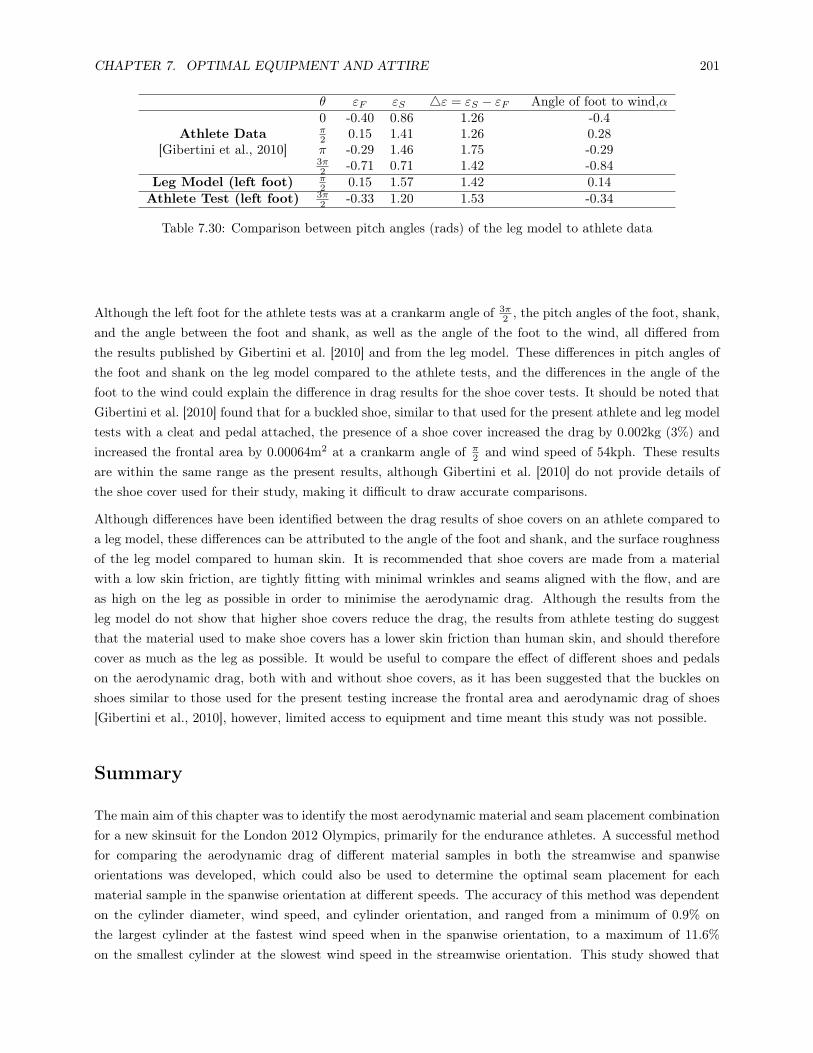
CHAPTER 7. OPTIMAL EQUIPMENT AND ATTIRE 201
& .F .S '. = .S ! .F Angle of foot to wind,$0 -0.40 0.86 1.26 -0.4
Athlete Data $2 0.15 1.41 1.26 0.28
[Gibertini et al., 2010] * -0.29 1.46 1.75 -0.293$2 -0.71 0.71 1.42 -0.84
Leg Model (left foot) $2 0.15 1.57 1.42 0.14
Athlete Test (left foot) 3$2 -0.33 1.20 1.53 -0.34
Table 7.30: Comparison between pitch angles (rads) of the leg model to athlete data
Although the left foot for the athlete tests was at a crankarm angle of 3$2 , the pitch angles of the foot, shank,
and the angle between the foot and shank, as well as the angle of the foot to the wind, all di!ered fromthe results published by Gibertini et al. [2010] and from the leg model. These di!erences in pitch angles ofthe foot and shank on the leg model compared to the athlete tests, and the di!erences in the angle of thefoot to the wind could explain the di!erence in drag results for the shoe cover tests. It should be noted thatGibertini et al. [2010] found that for a buckled shoe, similar to that used for the present athlete and leg modeltests with a cleat and pedal attached, the presence of a shoe cover increased the drag by 0.002kg (3%) andincreased the frontal area by 0.00064m2 at a crankarm angle of $
2 and wind speed of 54kph. These resultsare within the same range as the present results, although Gibertini et al. [2010] do not provide details ofthe shoe cover used for their study, making it di"cult to draw accurate comparisons.
Although di!erences have been identified between the drag results of shoe covers on an athlete compared toa leg model, these di!erences can be attributed to the angle of the foot and shank, and the surface roughnessof the leg model compared to human skin. It is recommended that shoe covers are made from a materialwith a low skin friction, are tightly fitting with minimal wrinkles and seams aligned with the flow, and areas high on the leg as possible in order to minimise the aerodynamic drag. Although the results from theleg model do not show that higher shoe covers reduce the drag, the results from athlete testing do suggestthat the material used to make shoe covers has a lower skin friction than human skin, and should thereforecover as much as the leg as possible. It would be useful to compare the e!ect of di!erent shoes and pedalson the aerodynamic drag, both with and without shoe covers, as it has been suggested that the buckles onshoes similar to those used for the present testing increase the frontal area and aerodynamic drag of shoes[Gibertini et al., 2010], however, limited access to equipment and time meant this study was not possible.
Summary
The main aim of this chapter was to identify the most aerodynamic material and seam placement combinationfor a new skinsuit for the London 2012 Olympics, primarily for the endurance athletes. A successful methodfor comparing the aerodynamic drag of di!erent material samples in both the streamwise and spanwiseorientations was developed, which could also be used to determine the optimal seam placement for eachmaterial sample in the spanwise orientation at di!erent speeds. The accuracy of this method was dependenton the cylinder diameter, wind speed, and cylinder orientation, and ranged from a minimum of 0.9% onthe largest cylinder at the fastest wind speed when in the spanwise orientation, to a maximum of 11.6%on the smallest cylinder at the slowest wind speed in the streamwise orientation. This study showed that

CHAPTER 7. OPTIMAL EQUIPMENT AND ATTIRE 202
the optimal material selection and seam placement was dependent on the orientation and diameter of thecylinders as well as the wind speed, the results of which could be related to di!erent parts of the body of acyclist. The surface roughness and seam placement appeared to have a greater impact on the aerodynamicdrag compared to the thickness, stretch or weave of the material samples, and Material 2 appeared to be theonly material rough enough to cause a significant decrease in the drag coe"cient within the critical Reynoldsnumber range. An analysis of the stress-strain relationship for the di!erent material samples in the weft, warpand bias orientations showed that Material 2 failed in the weft orientation before maximum displacement.No other material failed, and Material 5 in the bias orientation showed a more gentle and linear stretchingforce, which would be beneficial when getting the skinsuit over the shoulders of a cyclist. The best choiceof material for the forearms of a cyclist travelling at 50-60kph in terms of aerodynamics was found to beMaterial 5, the best material on the upper arms was found to be Material 5 with the seam at 60° from thepoint of stagnation, and the best material for the thighs was found to be Material 2 with the seam at 0°, 30°,150° or 180° from the point of stagnation.
Once the best material and seam placement had been identified for the forearms, upper arms and thighs aprototype skinsuit was made, but only using Material 5 due to di"culties obtaining Material 2 (Material 5was the second best material in terms of aerodynamics on the upper arms and thighs). Although significantdi!erences were identified between materials on the circular cylinder models, these di!erences were nottransferred to a complete skinsuit design to the same extent; using the results from the cylinder tests aprototype skinsuit was developed and compared to the best, existing New Zealand skinsuit, for which theaerodynamic drag results did not di!er significantly. Nevertheless, for an initial prototype design it waspromising to see that the same aerodynamic drag could be achieved using the results from the cylinder tests,from which point only improvements can be made. Further development on the type of seam used, andthe use of zoned fabric may lead to an improvement in the prototype design, and a greater gain in athleteperformance.
Although no indepth study was carried out on the aerodynamic drag of cycling equipment, some simple,initial tests showed that frame modifications contributed to only 0.3% of the total aerodynamic drag of acyclist, pedal and strap combinations contributed to only 2.1% of the overall drag, and frame and wheelcombinations contributed to only 3% of the overall drag. Previous research has shown that disc wheels havea lower drag than spoked wheels at zero yaw, but the improvements that can be made to bicycle frames andwheels is small compared to gains that can be made from modifications to athlete position. Although aerohelmets have also been shown to have a lower drag than non-aero helmets at zero yaw, the high variabilitybetween athlete body shapes and sizes results in di!erences between the helmet with the lowest drag forindividual riders.
A comparison of shoe covers used by elite, track cyclists was carried out on athletes and on a leg model, butdi!erences in the actual drag results and in the trends was observed between these two methods, primarilydue to the di!erence in skin friction drag of the artificial leg compared to human skin. Nevertheless, theresults showed that shoe covers that are higher on the leg and that minimise wrinkles and recesses help toreduce the aerodynamic drag, and shoe covers where the seam was placed down the front-centre had a lowerdrag compared to similar shoe covers with the seam across the ankles. The influence of a zip at the rearof the shoe cover or the number of holes on the bottom of the shoe cover (for the cleat) did not appear toa!ect the aerodynamic drag. The typical degree of di!erence between di!erent shoe covers on an athlete andbetween shoe covers and no shoe covers was found to be & 2.5%.

Chapter 8
Optimal Athlete Position
Introduction
Although it has been suggested that a low, crouched position is the most aerodynamic cycling position [Kyle,2003a, Burke and Pruitt, 2003, Broker, 2003] there is limited information on the actual optimal set up for atrack cyclist that results in this aerodynamic position. This chapter aims to identify some of these factors,in particular the optimal handlebar width and height, hand position, and torso and shoulder angles, in orderto provide a more quantitative analysis of the optimal position for a track cyclist compared to the generalcomparisons already described in the literature.
8.1 Handlebar Width and Height
An analysis of the e!ect of the width and height of the handlebar extensions was made by measuring theaerodynamic drag of seven elite male cyclists and seven elite female cyclists in their current, favoured racingposition, and then independently adjusting the separation of the elbow pads and the height of the handlebarsfrom their current favoured position. The degree to which the adjustments were made were dependent onthe athlete, their current racing position, and the equipment used; not all handlebars had the same amountof adjustment to the pad separation and/or height. The handlebars were raised or lowered using spacers onthe stem, and the elbow pads were placed wider apart or closer together using the adjustment slots on thepads. Each athlete was asked to pedal at a cadence of 100rpm, and all tests were carried out at a wind speedof 42kph and the drag results converted for an actual cycling speed of 60kph for the male cyclists and 50kphfor the female cyclists using Equation 8.1. The athletes were told to maintain a position that they couldcomfortably ride in for each handlebar change, which may have also resulted in a change in head position inorder to maintain their line of vision. The drag area was calculated for each athlete in each position usingEquation 8.2, where D is the measured drag (N), " is the air density (kgm3) and V is the velocity (ms!1).The drag readings were accurate to ±1%, the air density accurate to ±0.4%, and the velocity accurate to±0.13%. This gives a drag area accuracy of ±1.1%
($CdACdA
='(0.01)2 + (0.004)2 + (2" 0.013)2
).
The results for drag area were plotted to identify the optimal handlebar position for each athlete. Theseresults are shown in Figure 8.1 for the male athletes and Figure 8.2 for the female athletes.
203
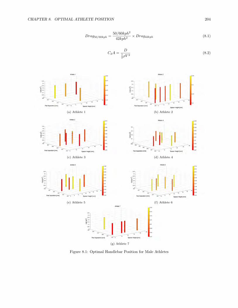
CHAPTER 8. OPTIMAL ATHLETE POSITION 204
Drag50/60kph =50/60kph2
42kph2"Drag42kph (8.1)
CdA =D
12"V
2(8.2)
(a) Athlete 1 (b) Athlete 2
(c) Athlete 3 (d) Athlete 4
(e) Athlete 5 (f) Athlete 6
(g) Athlete 7
Figure 8.1: Optimal Handlebar Position for Male Athletes

CHAPTER 8. OPTIMAL ATHLETE POSITION 205
(a) Athlete 1 (b) Athlete 2
(c) Athlete 3 (d) Athlete 4
(e) Athlete 5 (f) Athlete 6
(g) Athlete 7
Figure 8.2: Optimal Handlebar Position for Female Athletes
The results in Figures 8.1 and 8.2 show that the optimal handlebar position varies between all athletes, andthat there is no noticeable trend between the position with the lowest drag for all male or all female athletes.However, these results do show the influence of the handlebar separation and height individually on the drag,and that there is one specific handlebar position that produces the lowest drag area for each athlete. Tables8.1 and 8.2 show a summary of the position with the lowest drag (best position) and highest drag (worstposition) for each male and female athlete respectively, and also whether the greatest change in drag was froma change in bar height or pad separation. The handlebar separation was classified into narrow (<230mm formale athletes, <210mm for female athlete), mid (230-260mm for male athletes, 210-250 for female athletes)and wide (>260mm for male athletes, >250mm for female athletes) for each athlete in order to help identify

CHAPTER 8. OPTIMAL ATHLETE POSITION 206
if there were any trends. The di!erence in classification between male and female athletes was due to thedi!erence in handlebars used.
Male Athletes
Best Position Worst PositionAthlete Spacer Pad Spacer Pad !dragmax
Height (mm) Width Height (mm) Width due to
1 40 wide 0 wide bar height
2 5 narrow 35 narrow bar height
3 15 mid 25 mid bar height
4 0-10 mid 20 narrow/mid both
5 5 mid 20 mid bar height
6 10 mid 0 or 50 mid/wide bar height
7 5-25 narrow 15 wide bar width
Table 8.1: Handlebar Position with the Lowest Drag for Male Athletes
Female Athletes
Best Position Worst PositionAthlete Spacer Pad Spacer Pad !dragmax
Height (mm) Width Height (mm) Width due to
1 10 wide 30 wide bar height
2 0 narrow 0 wide bar width
3 30 wide 20 mid both
4 5-20 narrow 20 mid/wide bar width
5 0 or 30 narrow or wide 5 or 25 narrow or wide both
6 5 mid 25 mid bar height
7 10 narrow 10 mid bar width
Table 8.2: Handlebar Position with the Lowest Drag for Female Athletes
It was expected that the lowest drag would be seen for the lowest and narrowest handlebar setup, as thiswould relate to a low, crouched position which has been described as being the optimal cycling position inthe literature. However, the results show that although a relatively low handlebar position (between 0-20mmspacer height) resulted in the lowest drag for most of the athletes tested (71%) the handlebar separation forwhich the lowest drag was identified varied signficantly between the athletes. In general, a low handlebarposition results in a lower aerodynamic drag due to the reduction in frontal area as the athlete gets lower.However, for some athletes it is likely that a handlebar height that is too low causes the athlete to raiserather than lower their head, as they cannot maintain their line of vision. This could be a reason why thelowest handlebar height did not result in the lowest drag for all athletes. A handlebar height with spacersof 20mm or more appeared to result in the highest aerodynamic drag for just more than half of the athletes(57%) again indicating that a relatively low handlebar position is optimal in terms of aerodynamics. Thereis no clear indication of the optimal pad separation for the athletes used as subjects for this study; althougheach athlete had a pad separation that yielded a minimum drag, this separation varied between the athletes.

CHAPTER 8. OPTIMAL ATHLETE POSITION 207
This variability between optimal pad separation is most likely due to the di!erence in body sizes of athletes,as well as the athlete’s ability to maintain a low head position when the handlebars are narrow; athletes withwider shoulders may find it easier to maintain a low head position with wider handlebars, and handlebarsthat are too narrow for these athletes may in fact cause the athlete to raise their head and shoulders, causingan increase in frontal area. With narrow extensions a large proportion of the flow is directed around the body,but with wider extensions the flow passes over the handlebars, beneath the chest, between the legs, and acrossthe seat tube towards the rear wheel [Broker, 2003]. This suggests it is better to have narrow extensionsthan wide extensions, but the results in Table 9.3 indicate that some athletes actually benefit from havingslightly wider extensions. It is likely that the separation of the extensions should be set in proportion to theshoulder width in order to direct the flow around the body; for athletes with wide shoulders the extensionsshould be slightly wider than for athletes with narrow shoulders. In addition, narrow extensions may limitthe lung expansion and steering control, and may also a!ect the athlete’s ability to lower the head whilstmaintaining their line of vision.
In order to determine whether or not there was a correlation between aerodynamic drag and head position,the distance from the highest point on the helmet to the top of the extensions was measured from side imagestaken during testing for each athlete in each position, as shown in Figure 8.3. The camera was placed in thesame position for each test for each athlete, with no zoom, and the number of pixels determined for a knownheight of the bike stands in each image. This enabled the distance from the highest point on the helmet tothe top of the handlebar extensions to be calculated from pixels to millimetres. The results were then plottedagainst percentage change in drag area from the reference position for each athlete, to determine whether anincrease in head height resulted in a greater aerodynamic drag, as shown in Figure 8.4.
Figure 8.3: Measuring the distance between the highest point on the helmet to the top of the handlebarextensions from side images

CHAPTER 8. OPTIMAL ATHLETE POSITION 208
Figure 8.4: Relationship between drag area and head position
Figure 8.4 shows that there is no significant correlation between head position and drag area, i.e. head positionalone is not a good indicator of drag. It is likely that athletes adopt a head position that is comfortable,and this will vary between athletes due to di!erences in body size and shape. The choice of head position inrelation to handlebar position appears to be athlete specific, and may have been made in conjunction withother body position changes during their career. These other body position changes may mitigate the e!ectof head position on drag.
Although no correlation between aerodynamic drag and head position has been identified, by analysing boththe pad height and separation independently it is possible to determine the optimal handlebar setting foreach athlete. These results indicate that it is more important to optimise the handlebar height, after whichthe athlete can adopt a handlebar separation that is most comfortable and which allows them to maintain alower head position whilst still being able to maintain their line of vision. As there is no universal, optimalhandlebar setting due to di!erences in body sizes of athletes, it is important to assess each athlete individuallyin order to minimise their drag.
Table 8.3 shows the maximum percentage di!erence in drag from the reference position for each athlete whenchanging the height of the handlebars and separation of the elbow pads. These results again show the highvariability between the optimal handlebar position for athletes, as well as the variability between actual gainsand losses for athletes when making the same handlebar change. It is therefore important to recognise thatalthough trends may be seen, for example that the handlebar height has a slightly greater impact on dragthan the handlebar separation, the actual gains or losses made by individual athletes will vary. For futurestudies it would be useful to determine whether there is a trend between anthropometric characteristics, suchas shoulder width, and the optimal handlebar position for cyclists.

CHAPTER 8. OPTIMAL ATHLETE POSITION 209
Male Athletes Female AthletesHeight Separation Height Separation
Athlete Up Down Narrow Wide Athlete Up Down Narrow Wide1 2.4 4.1 3.7 baseline 1 2.0 0.7 1.0 baseline2 -3.4 -5.7 baseline -2.5 2 baseline 1.2 0.1 0.73 0.4 -1.6 -1.2 0.8 3 -1.4 baseline -1.9 baseline4 2.0 0.4 1.2 -1.2 4 1.8 0.5 -4.2 baseline5 1.2 0 -0.4 0 5 1.4 baseline 1.0 baseline6 0 -4.1 0.4 2.4 6 baseline -1.0 baseline -1.07 -0.1 -0.9 baseline 1.8 7 0.1 baseline 0.9 baseline
Table 8.3: Maximum percentage di!erence in drag from reference position
8.2 Hand Position
The position of the hands and forearms when riding with aerobars has an important e!ect on the aerodynamicdrag of cyclists, as this is the first point of contact for the flow of air around the athlete. However, competitiveand elite track cyclists do not all adopt the same hand position when racing in similar events. It appears thatriders tend to adopt a hand and forearm position depending on the type of aerobars used, and perhaps forindividual reasons relating to comfort and stability. Baker et al. [2001] researched the relationship betweenpower output and grip style, and Bressel and Cronin [2005] studied the relationship between the position ofthe hands on top and drops of handlebars and the pressure on the seat. However, there is limited informationin the literature about hand positions which reduce the aerodynamic drag on aerobars without compromisingpower output or stability. The aim of this study was to determine those hand positions which reduceaerodynamic drag and increase or maintain power output, therefore resulting in a significant time saving fortrack cyclists.
Eight healthy, elite, New Zealand track cyclists (5 male and 3 female) between 20 and 26 years of age, wereused as subjects for this study. All athletes used their own equipment, including track bike, handlebars,skinsuit and helmet, and adopted their own racing position on the bike apart from their hand position. Theathletes were placed on the cycle rig in the boundary layer wind tunnel at the University of Canterbury andthe wind speed set at 41kph. The athletes were asked to pedal at a cadence of 90rpm for each test, and wereinstructed to adopt each of the four di!erent hand positions shown in Figure 8.5. The aerodynamic dragand power output were recorded for each athlete in all hand positions. For each athlete, the di!erences indrag and average power output between (a) the normal hand position, and the other three hand positions (b)thumbs inside, (c) fist grip, and (d) arrow grip, were determined and the drag values extrapolated to 56kphor 53kph for male or female athletes respectively using Equation 8.3. An estimation of the time to complete a250m lap on an indoor velodrome, with zero wind and zero gradient, was determined using Equations 8.3, 8.4and 8.5, assuming an average pedalling speed of 56kph for male athletes and 53kph for female athletes. Thetime gain for hand positions (b), (c) and (d) relative to the normal hand position (a) was then determinedusing Equations 8.6 and 8.7, where Dwind is the drag force measured at wind speed (N), Dactual is the drag atthe average pedalling speed of the cyclist (N), Vwind is the velocity of the wind (m/s), Vactual is the averagepedalling speed of the cyclist (m/s), CdA is the product of drag coe"cient and frontal area of the rider (m2),

CHAPTER 8. OPTIMAL ATHLETE POSITION 210
CdAbaseline is the product of drag coe"cient and frontal area (m2) in the normal hand position (a), $ is theair density (kg/m3), g is the acceleration due to gravity (m/s2), T is the estimated finishing time (s), d isthe event distance (m), and P is the power output of the cyclist measured at the torque transducer at windspeed (W). A positive value for the time gain represents a time saving, whereas a negative number representsa time loss.
Figure 8.5: Hand positions (a) Normal (b) Thumbs inside (c) Fist grip (d) Arrow grip
Dactual =V 2actual
V 2wind
"Dwind (8.3)
CdA =Dwind12"V
2wind
(8.4)
T =d
3
,P
12!CdA
(8.5)
TimeGain(%) = 1!"
CdA
CdAbaseline
# 13
(8.6)
TimeGain(sec/min) = %" 3600
60(8.7)
Changes in position that resulted in increases or decreases in aerodynamic drag or power output were onlyconsidered relevant if the magnitude of the change was greater than 0.1N or 5W respectively. Smaller changeslie within the ±1% uncertainty of the drag and power measurement protocols and may mislead. The resultsfor aerodynamic drag, power output and time gain for all athletes in all hand positions tested are shown inTable 8.4.

CHAPTER 8. OPTIMAL ATHLETE POSITION 211
Hand Position (b) Thumbs Inside Hand Position (c) Fist Grip Hand Position (d) Arrow Grip
Athlete Time Gain Drag Power Athlete Time Gain Drag Power Athlete Time Gain Drag Power(sec/min) (N) (W) (sec/min) (N) (W) (sec/min) (N) (W)
7 1.14 -1.09 26 2 0.22 -0.186 -3 5 1.23 -1.17 3
2 0.25 -0.22 -2 3 0.16 -1.373 -23 2 0.79 -0.69 -15
6 0.09 -0.09 89 1 0.03 -0.029 -18 1 0.35 -0.34 -31
5 0.01 -0.01 -10 3 0.35 -0.30 -31
3 -0.01 0.01 -11
1 -0.11 0.11 3
8 -0.20 0.21 -149
4 -0.68 0.65 99
Table 8.4: Relationship between the time gain, drag and power output for changes in hand position from
Results in terms of aerodynamic drag
The fist grip (c) and arrow grip (d) hand positions both decreased the aerodynamic drag for all athletescompared to the normal hand position (a). Although the drag decreased significantly for athlete 7 whenadopting the thumbs inside hand position (b), the drag increased for all other athletes in this position. Thearrow hand position (d) was the most e!ective at reducing aerodynamic drag in general; the drag was reducedby 0.30-1.2N when athletes adopted the arrow grip hand position.
Results in terms of power output
Out of all the hand positions tested, only the thumbs inside hand position (b) resulted in an increase in poweroutput, but for only three of the athletes involved. The same hand position also resulted in a reduction inpower output for three other athletes, significantly so for athlete 8. Both the fist grip (c) and arrow grip (d)hand positions reduced the power output for all the athletes. The results show that a reduction in drag andcorresponding increase in power was seen for only athletes 6 and 7, and this was when the thumbs insidehand position (b) was adopted.
Results in terms of time gain
A positive value for time gain represents time saved and a negative value represents time lost. The fist grip(c) and arrow grip (d) hand positions both resulted in a time saving for all athletes tested. The arrow griphand position (d) resulted in the greatest time saving in general, of over 0.35sec/min for all athletes. Theonly noticable time loss was seen for the thumbs inside hand position (b), however, this same hand positionalso showed a significant time saving for athlete 7.
Relationship between drag, power and time gain
The greatest time saving (1.23 sec/min) was found when athlete 5 adopted an arrow hand position (d). Thiswas also the same athlete with the same hand position (d) where the lowest reduction in drag was observed(-1.167N). Although there was no noticeable increase in power output for athlete 5 in this hand position, thepower output did not decrease. The second greatest time saving (1.14 sec/min) was found when athlete 7adopted the thumbs inside hand position (b). This was also the same athlete and hand position with thesecond lowest drag reduction (-1.09N). For this athlete with this hand position there was also an increase of26W in power output. Similarly the athlete and hand position with the greatest time loss (-0.68sec/min) also

CHAPTER 8. OPTIMAL ATHLETE POSITION 212
had the highest increase in aerodynamic drag (0.647N). However, this athlete showed an increase in poweroutput by nearly 100W in this hand position (b). The results clearly show that for all hand positions (b),(c) and (d) there is a negative relationship between time gain and aerodynamic drag; the athlete with thegreatest time saving is also the athlete with the greatest reduction in drag for all hand positions. However,the results do not show a distinct relationship between power output and time gain or drag; the power outputincreases or decreases depending on the athlete and hand position adopted.
A visual analysis of the flow around the hands and forearms for each position tested was carried out byapplying cotton tufts, 30mm in length, to the hands and forearms of the skinsuit using ultra thin, clear,mylar tape. The flow pattern was captured for each hand position using a high speed video camera and thenanalysed. Images of the cotton tufts for each hand position can be seen in Figure 8.6.
(a) Normal hand position (b) Thumbs inside
(c) Fist grip (d) Arrow grip
Figure 8.6: Video analysis of hand positions using cotton tufts
For the normal (a) thumbs inside (b) and fist grip (c) hand positions the cotton tufts showed a smooth,steady flow pattern around all areas of the hands and forearms except for the region behind the thumbs,where the tufts showed separated flow. However, when the athletes adopted the arrow grip hand position (d)the cotton tufts in the region behind the thumbs were completely inverted, suggesting smooth recirculationoccurs. For all other areas of the hands and forearms in the arrow grip hand position (d) the flow remainedlaminar, similar to all other hand positions (a), (b) and (c).
This study has shown that there is a strong relationship between the hand position and time savings for acyclist through reduction in aerodynamic drag; optimal time savings are achieved when drag is reduced andpower is maximised. Aerodynamic drag can be reduced significantly by adopting an arrow style hand positionwhen riding with aerobars. Although there was no clear relationship between power output and drag or timegain, power output was reduced by less than 30W with the arrow style hand position. When adopting anarrow style hand position, a region of smooth recirculation developed in the area behind the thumbs. Thismay be more favorable than a region of turbulent separation, which was seen for all other hand positionstested. Although an arrow style hand position does not compromise the power output of athletes, the e!ectsof riding stability in this position needs further investigation before it can be concluded that this is a morebeneficial position for athletes. Baker et al. [2001] showed that when riding in unstable conditions power is

CHAPTER 8. OPTIMAL ATHLETE POSITION 213
used for changing the centre of mass rather than being applied directly to the cranks, which results in anoverall reduction in power output. There is a possibility that riders can train in a new hand position in orderto increase stability and power output for a hand position that has aerodynamic benefits. However, it can beconcluded that athletes should focus on minimising their aerodynamic drag together with maximising theirpower output in order to gain the most benefit in terms of time savings.
8.3 Torso and Shoulder Angle
The significance of body position on aerodynamic drag has been widely known for a number of years. Althoughmany studies have concluded that a low, crouched position where the frontal area is reduced also reducesthe aerodynamic drag, there is limited literature on the optimal angles of the hip, torso and shoulder fora track cyclist. Oggiano et al. [2008] found that drag was more sensitive to handlebar position than seatposition. Therefore the aim of this study was to determine the optimal position of a pursuit cyclist interms of aerodynamic drag and power output through changes in the elbow, shoulder and torso angles, asthese are the only angles a!ected by changes in handlebar position. The knee and hip angles are thereforekept constant, due to a constant seat position for each athlete. The UCI state that the forearms must behorizontal, the tip of the saddle behind the bottom bracket (BBB) must be 5cm maximum, and the distancefrom the bottom bracket to the end of the handlebars must be no more than 75cm [Regulations, 2009, version1.02.11]. These contraints limit the adjustability of the handlebars and saddle, which in turn a!ects the rangeof elbow, shoulder and torso angles. As the elbow angle is a function of the torso and shoulder angles, dueto the constraint that the forearms must be horizontal, it is only possible to analyse the e!ect of changes intorso and shoulder angles (together with changes in elbow angle) on the aerodynamic drag and power outputthrough adjustments made to the handlebars.
The angles which define the position of a cyclist are shown in Figure 8.7, where the knee angle, !, is the anglebetween the thigh and the lower leg, the hip angle, ", is the angle between the thigh and the horizontal, thetorso angle, #, is the angle between the torso and the horizontal, the shoulder angle, %, is the angle betweenthe torso and upper arm, and the elbow angle, &, is the angle between the upper arm and forearm.
Figure 8.7: Definition of angles of a cyclist

CHAPTER 8. OPTIMAL ATHLETE POSITION 214
In order to change the shoulder angle, a circle with the centre located at the shoulder point and which passedthrough the elbow joint was drawn, as shown in Figure 8.8a. The torso angle will remain the same for allpoints at which the elbow joint crosses this circle. In order to change the torso angle, a circle with the centrelocated at the hip point and which passed through the elbow joint was drawn, as shown in Figure 8.8b.The shoulder angle will remain the same for all points at which the elbow joint crosses this circle. Theserelationships are fixed because it is not possible to change the length of the upper body or forearms of acyclist.
(a) Shoulder angles (b) Torso angles
Figure 8.8: Changes in shoulder and torso angles
The e!ect of torso and shoulder angles on the aerodynamic drag and power output was analysed by using amodified handlebar setup, shown in Figure 8.9, consisting of an aluminium cylindrical rod of diameter 31.8mmand length 400mm, with Profile Design T1+ aerobars attached. Three athletes were used as subjects forthis study, each with their own equipment, except for the handlebar setup which was connected to eachbike using an Oval R710 adjustable stem of length 110mm, with 1mm spacers between the frame and stemfor adjustment. This setup allowed a complete range of torso and shoulder angles to be tested for thethree athletes. The shape of the handlebar extensions only allowed one wrist angle, which did not changethroughout the testing. The wind speed was set at 40kph (±0.03kph) for all tests. All tests were static(no pedalling) with the cranks in the horizontal orientation, although each athlete was told to pedal first toensure their position would be equivalent to how they would ride on a track. Details of each athlete can beseen in Table 8.5.

CHAPTER 8. OPTIMAL ATHLETE POSITION 215
Figure 8.9: Modified handlebar setup
Athlete1 2 3
Height (m) 173 178 177Weight (kg) 65 74 76
BMI 21.7 23.4 25Age (years) 16 27 45
Event Road and track 3-4km Road criterium 30-100km,track endurance 15-50km
Road cycling, time trial25-40km
Years in Discipline 2.5 9 20
Table 8.5: Athlete Details
White adhesive tape was placed on the athlete’s elbow, shoulder, hip, and wrist joints for identification ofthe di!erent angles. To locate the placement of the adhesive tape, the rider was asked to sit in their referenceposition and flex and extend each joint. The adhesive tape was placed at the point which moved the least.An additional marker was placed on the head tube of the bike to monitor adjustments of the handlebar. Alaser with a horizontal and vertical beam was used to ensure the handlebars were horizontal at this point.Each rider was asked to adopt their current racing position, and changes to the shoulder and torso angleswere made from this reference position. For each position, a side and rear photo was taken to record thestarting position and for measurement of the frontal area using a calibration stick with a 0.5m marked length.In addition, a shadow of the rider’s position from the side was projected on to a white board so that eachposition was controlled during testing, and so that the angle of the helmet to the horizontal remained thesame for each athlete. The distance between the handlebar extensions, the position of the hands on theextensions, and the location of the elbow pads were measured using the laser and a ruler for each test toensure these did not change and that the handlebars were always pointing forwards and were not tapered.An example of the test setup can be seen in Figure 8.10.

CHAPTER 8. OPTIMAL ATHLETE POSITION 216
Figure 8.10: Test setup
The side photos were imported into a CAD programme (Catia) and calibrated. Lines were then drawn toconnect the adjacent joint markers to display the current angles, as shown in Figure 8.11. To calculate thenecessary adjustment for the next testing position a sketch with changeable angles was drawn, which displayedthe distances to the previous elbow position. This method allowed not only the angles to be measured, butalso the necessary adjustments to the handlebar to be determined in order to obtain specific shoulder andtorso angles.
Figure 8.11: Side photo imported into Catia to determine the changes in shoulder and torso angles

CHAPTER 8. OPTIMAL ATHLETE POSITION 217
Each test was repeated, and the ambient air temperature and pressure was recorded before each test. Thereference position of each athlete was also repeated at the very end to verify the results. An SRM PowerMeter was fixed to each bike and the power data was collected without the wind while each rider pedalledat a cadence comfortable for themselves for 30 seconds. Although the riders were not able to hold the exactcadence for 30 seconds, a linear relationship could be assumed between power and cadence to determine theaverage power output at an average cadence. The wind trainer resistance could be adjusted in five incrementsand the same resistance was used for all riders. By calculating the power required by each rider to overcomethe measured drag in each position (Equation 8.8) assuming their gearing would allow them to achieve thisvelocity at the cadence they used in the wind tunnel tests, the surplus power was determined by subtractingthis value from the power output measured by the SRM in each position (Equation 8.9), where Crr is thecoe"cient of rolling resistance (0.002 for track cycling [Wilson, 2004]), g is the acceleration due to gravity(m/s2) and m is the total mass of the rider and bike (kg). The optimal position in terms of power output istherefore the position which results in the greatest surplus power. Surplus power is the power available foracceleration, gradient climbing etc.
Pd =1
2"CdAV 3 + CrrV (8.8)
Psurplus = Pmeasured ! Pd (8.9)
The drag area, CdA, and drag coe"cient, Cd, were calculated using Equations 8.10 and 8.11 respectively,where D is the measured drag force (N), " is the air density (kg/m3), V is the wind speed (m/s) and A isthe calculated frontal area of the rider and bike (m2).
CdA =2D
"V 2(8.10)
Cd =CdA
A(8.11)
Finally the relationship between the drag area and torso angle, and between the drag area to body mass ratioand torso angle was determined, for comparison to the results published by Garcia-Lopez et al. [2008].
Plots of the drag area against shoulder and torso angles were created to determine the optimal position interms of aerodynamic drag, where the lowest drag area is the optimum. These plots can be seen in Figure8.12 for each athlete tested. Table 8.6 shows the average drift between the recorded drag at the beginningand end of each test for each athlete, the maximum di!erence in drag between tests in the same position foreach athlete, and the greatest di!erence in drag between the best and worst position out of those tested foreach athlete.

CHAPTER 8. OPTIMAL ATHLETE POSITION 218
(a) Athlete 1 (b) Athlete 2
(c) Athlete 3
Figure 8.12: Drag area results
Average Drift Max Di!erence in Drag Di!erence between highest and lowest(g) for Same Position (g) drag in di!erent positions (g)
Athlete 1 6.1 20 200Athlete 2 14.7 52 270Athlete 3 6.0 40 180
Table 8.6: Drift and drag results for each athlete
Plots of the calculated surplus power against shoulder and torso angles were created to determine the optimalposition in terms of power output, where the highest surplus power is the optimum. Note that the poweroutput was taken at a cadence which was comfortable for each athlete. The results are shown in Figure 8.13.

CHAPTER 8. OPTIMAL ATHLETE POSITION 219
(a) Athlete 1 (Cadence 110rpm, Speed 12m/s) (b) Athlete 2 (Cadence 90rpm, speed 10m/s)
(c) Athlete 3 (Cadence 82rpm, speed 10m/s)
Figure 8.13: Results for Surplus Power
A summary of the torso and shoulder angles at which the minimum drag area and drag coe"cient, andmaximum power output and surplus power was found for each athlete are shown in Tables 8.7 and 8.8.
Torso Angle (°) ±1°Min Angle Tested Max Angle Tested CdAmin Cdmin Max Pout Max Psurplus
Athlete 1 5.0 13.3 8.6 8.6 7.3 8.6Athlete 2 6.8 19.3 6.8 7.4 6.8 6.8Athlete 3 1.6 16.2 1.6 9.0 4.5 4.5
Table 8.7: Torso angle (degrees) at which the minimum drag area and drag coe"cient, and maximum poweroutput and surplus power was found for each athlete
Shoulder Angle (°) ±3°Min Angle Tested Max Angle Tested CdAmin Cdmin Max Pout Max Psurplus
Athlete 1 93.3 108.6 105.3 105.3 93.3 105.3Athlete 2 84.3 99.3 90.7 84.9 90.7 90.7Athlete 3 85.0 92.9 92.9 90.8 88.9 88.9
Table 8.8: Shoulder angle (degrees) at which the minimum drag area and drag coe"cient, and maximumpower output and surplus power was found for each athlete
For athlete 1, the minimum drag area (CdA=0.260) occurred at a torso angle of 8.6˚ and shoulder angleof 105.3˚. However, the greatest power output (329.04W) occurred at a torso angle of 6.8˚ and shoulder
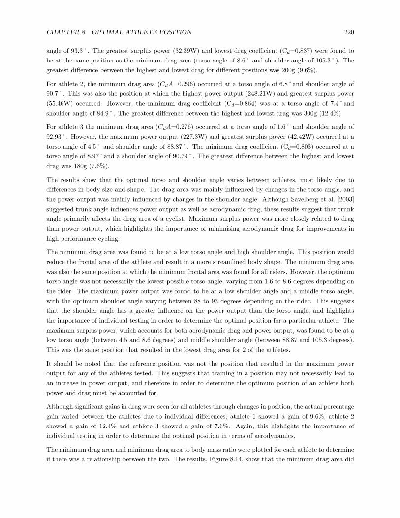
CHAPTER 8. OPTIMAL ATHLETE POSITION 220
angle of 93.3˚. The greatest surplus power (32.39W) and lowest drag coe"cient (Cd=0.837) were found tobe at the same position as the minimum drag area (torso angle of 8.6˚ and shoulder angle of 105.3˚). Thegreatest di!erence between the highest and lowest drag for di!erent positions was 200g (9.6%).
For athlete 2, the minimum drag area (CdA=0.296) occurred at a torso angle of 6.8˚and shoulder angle of90.7˚. This was also the position at which the highest power output (248.21W) and greatest surplus power(55.46W) occurred. However, the minimum drag coe"cient (Cd=0.864) was at a torso angle of 7.4˚andshoulder angle of 84.9˚. The greatest di!erence between the highest and lowest drag was 300g (12.4%).
For athlete 3 the minimum drag area (CdA=0.276) occurred at a torso angle of 1.6˚ and shoulder angle of92.93˚. However, the maximum power output (227.3W) and greatest surplus power (42.42W) occurred at atorso angle of 4.5˚ and shoulder angle of 88.87˚. The minimum drag coe"cient (Cd=0.803) occurred at atorso angle of 8.97˚and a shoulder angle of 90.79˚. The greatest di!erence between the highest and lowestdrag was 180g (7.6%).
The results show that the optimal torso and shoulder angle varies between athletes, most likely due todi!erences in body size and shape. The drag area was mainly influenced by changes in the torso angle, andthe power output was mainly influenced by changes in the shoulder angle. Although Savelberg et al. [2003]suggested trunk angle influences power output as well as aerodynamic drag, these results suggest that trunkangle primarily a!ects the drag area of a cyclist. Maximum surplus power was more closely related to dragthan power output, which highlights the importance of minimising aerodynamic drag for improvements inhigh performance cycling.
The minimum drag area was found to be at a low torso angle and high shoulder angle. This position wouldreduce the frontal area of the athlete and result in a more streamlined body shape. The minimum drag areawas also the same position at which the minimum frontal area was found for all riders. However, the optimumtorso angle was not necessarily the lowest possible torso angle, varying from 1.6 to 8.6 degrees depending onthe rider. The maximum power output was found to be at a low shoulder angle and a middle torso angle,with the optimum shoulder angle varying between 88 to 93 degrees depending on the rider. This suggeststhat the shoulder angle has a greater influence on the power output than the torso angle, and highlightsthe importance of individual testing in order to determine the optimal position for a particular athlete. Themaximum surplus power, which accounts for both aerodynamic drag and power output, was found to be at alow torso angle (between 4.5 and 8.6 degrees) and middle shoulder angle (between 88.87 and 105.3 degrees).This was the same position that resulted in the lowest drag area for 2 of the athletes.
It should be noted that the reference position was not the position that resulted in the maximum poweroutput for any of the athletes tested. This suggests that training in a position may not necessarily lead toan increase in power output, and therefore in order to determine the optimum position of an athlete bothpower and drag must be accounted for.
Although significant gains in drag were seen for all athletes through changes in position, the actual percentagegain varied between the athletes due to individual di!erences; athlete 1 showed a gain of 9.6%, athlete 2showed a gain of 12.4% and athlete 3 showed a gain of 7.6%. Again, this highlights the importance ofindividual testing in order to determine the optimal position in terms of aerodynamics.
The minimum drag area and minimum drag area to body mass ratio were plotted for each athlete to determineif there was a relationship between the two. The results, Figure 8.14, show that the minimum drag area did

CHAPTER 8. OPTIMAL ATHLETE POSITION 221
not coincide with the minimum drag area to body mass ratio, which is in agreement with the study byGarcia-Lopez et al. [2008] and suggests that body mass is not a significant factor in terms of drag reduction.
Figure 8.14: Relationship between the minimum drag area and drag area to body mass ratio for each athlete
Plots of drag area with change in torso angle, and drag area to body mass ratio with change in torso anglewere also generated to determine if there was any significant correlation. The results, shown in Figures 8.15and 8.16 respectively, indicate that there was a significant correlation between torso angle and drag area(r=0.6604) and a significant correlation between torso angle and drag area to body mass ratio (r=0.5973),which is also in agreement with the results published by Garcia-Lopez et al. [2008]. These results suggestthat a low torso angle reduces the drag area for riders of di!erent all body masses tested, but that body massis not a significant factor in terms of drag reduction.
Figure 8.15: Drag area as a function of torso angle

CHAPTER 8. OPTIMAL ATHLETE POSITION 222
Figure 8.16: Drag area to body mass ratio as a function of torso angle
It should be noted that drag was measured at a single speed. During a race the speed will vary, as will theReynolds number and drag coe"cient. The cyclists’ Reynolds number, taking the length scale as 1m, is oforder one million, and the drag coe"cient is not expected to vary much as the boundary layer over muchof the cyclist will be fully turbulent. However the drag contribution of individual elements exposed to theundisturbed wind, such as the helmet, arms and front wheel, may vary to a greater degree. Future studiesshould attempt to match the resistance applied to the wheels to the drag and rolling resistance experiencedat the speed simulated, and considering the gearing, ensure the cadence is appropriate to this speed. Higherspeeds should also be tested.
Summary
The aim of this chapter was to provide a more quantitative analysis of the optimal athlete position, inparticular for the handlebar width and height, hand position, and torso and shoulder angles. It has beenshown that the optimal position for an athlete is very individual, due to di!erences in body size and shape,although some trends do exists even though actual percentage gains and losses di!er between athletes. Theheight of the handlebars showed to have a slightly greater influence on the aerodynamic drag than thehandlebar height, with a low handlebar height (<20mm spacing under the stem) resulting in a lower drag forthe majority of athletes tested. A strong relationship was identified between hand position and time saving,with an arrow style hand position reducing the drag without compromising the power output. However,the stability of an arrow style hand position was questioned, suggesting that a further study was needed toidentify if athletes could train in this position and hold it for the duration of a race without feeling unstable.In terms of the torso and shoulder angle, the minimum drag area was identified at a low torso angle, but notnecessarily the lowest angle tested, and a high shoulder angle. The maximum power output was identified ata mid torso angle and low shoulder angle, suggesting that the shoulder angle has a greater influence on thepower output and the torso angle has a greater influence on the drag. The concept of surplus power was usedto identify the optimal torso and shoulder angle in terms of both drag and power output, and the results

CHAPTER 8. OPTIMAL ATHLETE POSITION 223
showed that the maximum surplus power for the athletes tested was at a low torso angle (4.5° to 8.6°) andmid shoulder angle (88.9° to 105.3°). The actual percentage gain varied between athletes, again highlightingthe importance of individual testing to identify the exact set up that results in the lowest drag and highestpower output for each athlete. For future studies it would be beneficial to identify whether any trends existbetween anthropometric data and the optimal position of individual athletes in terms of handlebar positionand torso and shoulder angles.

Chapter 9
Overall Gains and Losses
Introduction
The experimental results for all positional and equipment changes described in Chapters 7 and 8 werecombined so that the potential gains to be had from optimising equipment and/or position could be ranked.As not all tests included pedalling athletes as subjects, a comparison was made between stationary andpedalling tests for the same changes in position and equipment (using the same athletes) to determinewhether there was a significant di!erence between the percentage gains or losses in drag for changes madeusing pedalling athletes compared to stationary athletes. Two athletes compared stationary and pedallingtests for changes made to athlete position, one athlete compared stationary and pedalling tests for di!erentskinsuits, and one athlete compared stationary and pedalling tests for di!erent shoe covers. The wind tunnelwas set at 42kph for all tests and the results can be seen in Table 9.1.
224

CHAPTER 9. OVERALL GAINS AND LOSSES 225
Drag Static % Di!erence Drag Pedalling % Di!erence % Di!erenceAthlete Test (kg) from (kg) from Pedalling
Baseline Baseline vs Stationary
Baseline 1.831 - 2.012 - -
Bars down 10mm 1.974 7.2 2.155 6.6 -0.6
1 Longer extensions 1.957 6.4 2.135 5.8 -0.7
Wider bars 2.054 10.9 2.262 11.1 0.2
Narrower bars 2.034 10.0 2.254 10.7 0.8
Baseline 2.001 - 2.055 - -
Bars lower 1.942 -3.0 1.978 -3.9 -0.9
2 Extensions 20mm higher 1.981 -1.0 2.022 -1.6 -0.6
Bars 10mm lower 1.952 -2.5 2.001 -2.7 -0.2
Helmet change 1.986 -0.8 2.037 -0.9 -0.1
Skinsuit 1 1.972 - 2.102 - -
3 Skinsuit 2 1.988 0.8 2.106 0.2 -0.6
Skinsuit 3 2.030 2.9 2.153 2.4 -0.5
Skinsuit 4 1.965 -0.4 2.079 -1.1 -0.8
No Shoe Covers 2.134 2.209
4 Prototype 1 2.083 -2.4 2.154 -2.6 -0.1
Prototype 2 2.089 -2.2 2.172 -1.7 0.5
Champion Systems 2.130 -0.2 2.200 -0.4 -0.2
Table 9.1: Comparison between pedalling and stationary tests for the same changes in position and equipment
The results from Table 9.1 show that the di!erence in the percentage gains and losses between pedalling testscompared to stationary tests was <±1%, which is the same as the uncertainty of the cycle rig. Therefore itcan be assumed that the percentage gains and losses for stationary tests are the same as for pedalling tests,and so all experimental results for changes in position and equipment described in Chapters 7 and 8, whetherstationary or pedalling, will be included in the overall ranking of potential gains to be had from optimisingequipment and/or position. The only experimental results that will be omitted are those where no athletewas used for testing (shoe covers on a leg model and material testing for skinsuits).
In addition to the detailed wind tunnel tests described in Chapters 7 and 8, a number of individual andmultiple changes in position and equipment were carried out on elite athletes in the wind tunnel with theoverall aim of identifying the optimal set up for individual track cyclists. All athletes were pedalling atapproximately 90rpm for each change made, and the wind tunnel speed was set at 42kph. Individual changesin position included changes to the bar height, bar width, bar length, seat height, seat lateral position, helmettip position, degree of tapering to the bars, and lowering the head into a more crouched position. Multiplechanges in position were made by combining one or more of the individual changes mentioned. Equipmentchanges included testing di!erent skinsuits, di!erent helmets, taping helmet holes, comparing shoe covers tono shoe covers, and tucking long hair into the helmet or in a bun to eliminate the hair from the oncoming flow.All changes were made from the reference position of each athlete, and the di!erence in drag recorded. Notevery athlete compared all changes in position and/or equipment due to di!erences in equipment, referenceposition, and time constraints. Also, as the position of the seat is related to the athlete’s leg length, a changein seat height was only considered worthwhile if the athlete believed that they could produce the same orgreater power output. No athlete believed that they could produce the same or greater power with a lowerseat, so therefore this change in position was not carried out.

CHAPTER 9. OVERALL GAINS AND LOSSES 226
In order to determine the impact of each change on the aerodynamic drag, the greatest di!erence in drag fromthe reference position (gain or loss) was recorded for each change for each athlete. The reference position waschosen to be the current racing position for each individual athlete, including their own bike, wheels, helmetand skinsuit. Although the actual setup varied between athletes, most athletes adopted a relatively low, aeroposition using handlebar extensions and wearing an aero helmet. The average impact of each change on theaerodynamic drag could then be calculated. For this analysis the degree to which changes were made, forexample the actual angle of the helmet tip to the horizontal or the actual degree of tapering of the bars,was not important, as the aim was to determine the impact of each change on the drag and not to comparethe actual position or equipment used between athletes. The average impact on drag was separated intoindividual, multiple, and equipment changes because it cannot be assumed that gains and losses are additive;the flow field around an athlete is not a linear superposition of component flow fields. The approximatetime saving for each change in position and/or equipment was then calculated using the mathematical modeland the data for one of the male athletes used to validate the model (Athlete 11) described in Chaper 4;percentage changes in drag area, CdA, made on other athletes were applied to the drag area of Athlete 11in the model. Any trends between changes in position and/or equipment with gender, competitive level, orbetween road and track cyclists were identified by categorising the data and generating plots to compare theaverage change in drag from the reference position for each category. This chapter aims to identify the mostsignificant factors in terms of aerodynamic drag, to help athletes and coaches quickly identify those areaswhere performance gains can be made and to quantify these gains in terms of an approximate time saving.
9.1 Calculation of Time Saving
The mathematical model described in Chapter 4 was used to calculate the finishing time for each change inposition and/or equipment using the data for one of the athletes used to validate the model (Athlete 11). Asummary of the data for Athlete 11 can be seen in Table 9.2.

CHAPTER 9. OVERALL GAINS AND LOSSES 227
Data for Athlete 11 (male, elite, track cyclist)Measured Dragwindtunnel (at 42kph) (N) 29.07
Temperature (°C) 28Pressure (mbar) 1021
Relative Humidity (%) 60Air density (kg/m3) 1.1806
Average velocity (kph) 55Height (m) 1.85Weight (kg) 75
Seat height (m) 1.2Drag area, CdA (m2) 0.195
Gear Ratio 3.8Drive chain e"ciency (%) 98
Frame Mass (kg) 8Wheel Mass (kg) 1.255Wheel Radius (m) 0.3315Bearing Radius (m) 0.012
Tyre Coe"cient of Rolling Resistance (Crr) 0.002Bearing Coe"cient of Rolling Resistance (Crr) 0.002
Increase in Rolling Resistance in Bends (scrubbing) (%) 28Increase in Rolling Resistance in Straights (scrubbing) (%) 4
Percentage Weight on Rear Wheel (%) 60Track Grade Angle (rad) 0
Track Banking Angle in Straights (rad) 0.733Track Banking Angle in Bends (rad) 0.22
Track Radius of Curvature in Bends (m) 26.101Track Radius of Curvature in Straights (m) 1x10²¹
Race distance (m) 4000Actual finishing time (s) 265.023
Predicted finishing time (s) 268.370
Table 9.2: Data for Athlete 11 used to calculate the approximate time saving for each change in positionand/or equipment
For each change made to the position or equipment the change in drag area, CdA, from the reference positionwas calculated from the measured drag results using Equation 9.1, where 'D is the change in measured dragfrom there reference position (N), " is the air density (kgm!3) and V is the wind speed (ms!1). This enableda new drag area to be inserted into the mathematical model, while all other inputs remained the same, inorder to calculate the time di!erence between each change and the reference position for a 4000m IndividualPursuit event.
'CdA ='D12"V
2(9.1)
9.2 Rank of Changes in Terms of Impact on Drag
The maximum change in drag from the reference position (increase or decrease) for each variable tested (e.g.stem height) for each athlete was averaged and these results were then ranked in terms of impact, i.e. from

CHAPTER 9. OVERALL GAINS AND LOSSES 228
highest to lowest gains or losses. These results for individual, multiple, and equipment changes can be seen inTables 9.3, 9.4 and 9.5 respectively. The time savings for each individual change in position, multiple changein position, and equipment change for a 4000m IP athlete are shown in Tables 9.6, 9.7 and 9.8 respectively.Change in drag means the di!erence in drag force from the reference position (N). A more detailed descriptionof each change can be seen in Appendix E.

CHAPTER 9. OVERALL GAINS AND LOSSES 229
Maxim
um
per
centa
ge
change
indra
g(+
or
-)
from
the
refe
rence
posi
tion
for
each
,in
div
idualath
lete
(1to
25)*
Av.!
dra
g
Change
12
34
56
78
910
11
12
13
14
15
16
17
18
19
20
21
22
23
24
25
(%)
Hea
dlo
w/cr
ouch
3.8
0.7
5.1
3.7
0.7
4.2
6.5
2.2
2.3
4.4
2.6
5.4
3.5
Hel
met
tip
up
4.1
2.3
2.4
1.9
2.7
Exte
nsi
ons
short
ened
1.7
3.2
2.5
Hand
change
0.5
3.3
0.4
1.6
3.5
3.0
4.1
0.9
2.1
1.6
2.1
Tip
dow
n4.3
2.5
2.4
2.1
1.9
0.5
1.4
1.1
2.0
2.0
Ste
mdow
n0.5
0.4
0.7
2.8
1.3
2.3
1.0
1.6
3.9
4.1
5.7
0.5
1.2
2.0
Sea
tback
1.8
1.8
Hair
tuck
edin
2.5
1.0
1.8
Sea
tfo
rward
s1.7
1.7
Exte
nsi
ons
wid
er0.6
1.2
0.2
1.4
1.2
1.0
5.4
0.8
2.4
2.5
0.7
1.6
Ste
mup
2.0
2.0
1.9
0.1
1.4
2.0
1.9
1.4
0.4
1.2
0.8
1.2
3.4
1.2
1.8
1.5
Taper
edbars
0.3
2.6
1.7
1.6
1.3
2.4
3.0
0.4
0.2
1.5
Exte
nsi
ons
narr
ower
1.2
15.4
0.9
0.1
1.0
1.9
1.2
0.4
0.4
4.2
0.1
1.5
Exte
nsi
ons
length
ened
1.3
1.2
1.7
1.6
1.5
Rais
ese
at
0.1
1.3
1.5
1.0
Tabl
e9.
3:R
ank
ofG
ains
orLo
sses
inD
rag
for
each
Indi
vidu
alC
hang
ein
Posi
tion
per
athl
ete
*The
sear
eth
em
axim
umch
ange
sin
drag
(inc
reas
eor
decr
ease
)fr
omth
ere
fere
nce
posi
tion
for
each
athl
ete
for
each
vari
able
test
ed.

CHAPTER 9. OVERALL GAINS AND LOSSES 230
Maxim
um
change
indra
g(%
)fr
om
refe
rence
posi
tion
for
each
ath
lete
Av!
dra
g
Change
12
34
56
78
910
11
12
13
14
15
16
17
18
19
20
21
22
23
(%)
Exte
nsi
on
hei
ght
and
length
9.6
11.1
7.6
9.4
Hel
met
tip
up
&st
emdow
n4.6
4.6
Ste
mdow
n&
hand
change
6.1
1.8
4.0
Exte
nsi
ons
forw
ard
&hea
dlo
w5.1
3.5
0.7
6.2
3.9
Exte
nsi
on
hei
ght
and
wid
thw
ith
hea
dlo
w2.4
4.6
4.8
3.9
Ste
mdow
n&
hea
dlo
w2.2
4.7
3.5
Exte
nsi
ons
wid
er&
hea
dlo
w4.1
1.0
2.6
Exte
nsi
ons
forw
ard
&narr
ow1.0
3.4
2.2
Sea
tra
ised
&st
emdow
n1.7
1.7
Exte
nsi
on
hei
ght
and
wid
th0.5
1.9
3.8
0.6
1.7
Bars
taper
ed&
hand
change
2.7
0.5
1.6
1.6
Exte
nsi
ons
forw
ard
&hand
change
2.3
0.9
1.6
Tabl
e9.
4:R
ank
ofG
ains
orLo
sses
inD
rag
for
each
Mul
tipl
eC
hang
ein
Posi
tion
per
Ath
lete

CHAPTER 9. OVERALL GAINS AND LOSSES 231
Maxim
um
change
indra
g(%
)fr
om
refe
rence
posi
tion
for
each
ath
lete
Av!
dra
g
Change
12
34
56
78
910
11
12
13
14
15
16
17
18
19
20
21
22
23
24
25
(%)
Di!
eren
tsk
insu
it2.3
4.5
7.6
2.0
8.0
8.9
7.6
7.7
7.7
6.3
Di!
eren
tfr
am
e&
whee
ls*
3.0
3.0
Di!
eren
thel
met
3.7
3.2
1.8
3.3
2.8
6.2
1.2
1.2
2.9
Sam
ew
hee
lsdi!
eren
tfr
am
e*2.8
2.8
Sam
efr
am
edi!
eren
tw
hee
ls*
2.5
2.5
Vis
or
vs
no
vis
or
2.2
1.8
3.0
0.2
4.7
2.8
1.7
3.4
2.4
0.2
2.7
1.5
2.2
Ped
al/
stra
pco
mbin
ati
on
2.1
2.1
Shoe
cover
svs
no
shoe
cover
s2.4
1.5
1.7
1.7
1.8
1.8
Sam
eped
aldi!
eren
tst
rap
1.8
1.8
Glo
ves
vs
no
glo
ves
1.3
1.3
Hel
met
hole
sta
ped
vs
unta
ped
1.0
0.7
0.9
Sam
est
rap
di!
eren
tped
al
0.3
0.3
Modifi
edse
at
tube
shape
0.3
0.3
Modifi
edfo
rksh
ape
0.2
0.2
Modifi
edSte
msh
ape
0.1
0.1
Tabl
e9.
5:R
ank
ofG
ains
orLo
sses
inD
rag
for
each
Equ
ipm
ent
Cha
nge
per
Ath
lete
*W
heel
sw
ere
disc
whe
els.

CHAPTER 9. OVERALL GAINS AND LOSSES 232
Change Average ! Drag (%). ! CdA ! Time
Tucked head/crouch/head low 3.5 0.0068 2.940
Helmet tip up 2.7 0.0053 2.520
Extensions shortened 2.5 0.0049 2.105
Hand change 2.1 0.0041 1.690
Tip down 2.0 0.0039 1.690
Stem down 2.0 0.0039 1.690
Seat back 1.8 0.0035 1.690
Hair tucked in 1.8 0.0035 1.690
Seat forwards 1.7 0.0033 1.690
Extensions wider 1.6 0.0031 1.270
Stem up 1.5 0.0029 1.270
Tapered bars 1.5 0.0029 1.270
Extensions narrower 1.5 0.0029 1.690
Extensions lengthened 1.5 0.0029 1.270
Raise seat 1.0 0.0020 0.850
Table 9.6: Calculated Time Savings for Each Individual Change in Position from the Reference Position
Change Average ! Drag (%). ! CdA ! Time
Extension height and length 9.4 0.0183 8.180
Helmet tip up & stem down 4.6 0.0090 4.170
Stem down & hand change 4.0 0.0078 3.350
Extensions forward & head low 3.9 0.0076 3.350
Extension height and width with head low 3.9 0.0076 3.350
Stem down & head low 3.5 0.0068 2.940
Extensions wider & head low 2.6 0.0051 2.105
Extensions forward & narrow 2.2 0.0043 2.105
Seat raised & stem down 1.7 0.0033 1.690
Extension height and width 1.7 0.0033 1.690
Bars tapered & hand change 1.6 0.0031 1.270
Extensions forward & hand change 1.6 0.0031 1.270
Table 9.7: Calculated time savings for Multiple Changes in Position from the Reference Position

CHAPTER 9. OVERALL GAINS AND LOSSES 233
Change Average ! Drag (%). ! CdA ! Time
Di!erent skinsuit 6.3 0.0123 5.370
Di!erent frame & wheels 3.0 0.0059 2.520
Di!erent helmet 2.9 0.0057 2.520
Same wheels di!erent frame 2.8 0.0055 2.520
Same frame di!erent wheels 2.5 0.0049 2.105
Visor vs no visor 2.2 0.0043 2.105
Pedal/strap combination 2.1 0.0035 1.690
Shoe covers vs no shoe covers 1.8 0.0035 1.690
Same pedal di!erent strap 1.8 0.0035 1.690
Gloves vs no gloves 1.3 0.0031 1.270
Helmet holes taped/untaped 0.9 0.0018 0.850
Same strap di!erent pedal 0.3 0.0006 0.425
Modified seat tube shape 0.3 0.0006 0.425
Modified fork shape 0.2 0.0004 0.000
Modified Stem shape 0.1 0.0002 0.000
Table 9.8: Calculated time savings for Equipment Changes
The individual change in position that had the greatest impact on drag came from adopting a crouch position,where the head was lowered into the shoulders while ensuring the cyclists continue to look forwards andmaintain their line of vision, with an average of a 3.5% change in drag from the reference position and atime saving of 2.94s over 4000m. The multiple change in position that had the greatest impact on drag camefrom changing the extension height and length, with an average of a 9.4% change in drag from the referenceposition and a time saving of 8.18s over 4000m. The equipment change that had the greatest impact ondrag was a change in skinsuit, with an average of a 6.3% change in drag from the reference position and atime saving of 5.37s over 4000m. By adopting a crouch position athletes are able to reduce their frontal areasignificantly, and previous published results have shown that there is a strong correlation between frontalarea and aerodynamic drag [Defraeye et al., 2010]. A change to the height and length of the extensions hasan influence on the torso and shoulder angle of a cyclist, and by lengthening the extensions and loweringthe handlebars it is possible to bring the torso closer to the horizontal, which has also been shown to helpreduce the aerodynamic drag significantly [Kyle, 2003a] and reduce the frontal area. A change in skinsuitcan a!ect both skin friction drag and pressure drag through the use of a di!erent material, seam placement,and fit (number of wrinkles). By strategically placing material and seams on di!erent parts of the body itis possible to induce turbulence and delay separation, which consequently reduces the drag. Minimising thenumber of wrinkles and ensuring the skinsuit is a tight fit will also help reduce the drag, and the results inthis study have shown how great an impact a skinsuit can have in terms of athlete performance.
The results from this study show that in general, multiple changes result in a greater gain or loss in dragcompared to individual changes, probably because multiple changes in position reduce the frontal area morethan individual changes in position. However, that the gains and losses are not additive; a combination ofthe individual changes which result in the greatest di!erence from the reference position will not necessarilyresult in the greatest di!erence for multiple changes, nor will the total gain or loss be an addition of theindividual gains or losses. For example individual changes made by moving the stem down and lowering headresulted in an average change in drag from the reference position of 2.0% and 3.5% respectively, but whencombined as a multiple change in position the average change in drag from the reference position was 5.5%.

CHAPTER 9. OVERALL GAINS AND LOSSES 234
A change in skinsuit had a significantly greater impact on the aerodynamic drag compared to all other changesmade to the equipment, and a change to the shape of the bike frame had no significant impact on the drag(<0.3%). This low change in drag for the bike frame is likely to be due to the fact that all bikes used in thisstudy were already optimised in terms of aerodynamics with an aerodynamic frame; a comparison between anon-aerodynamic and aerodynamic frame would likely lead to a greater change in drag. In general, changes inposition had a greater impact on drag compared to changes in equipment, which is in agreement with previousstudies that state that athlete position is the most influential factor on aerodynamic drag when cycling onthe flat at speeds greater than 13kph [Kyle, 2003a]. However, certain changes made to the equipment alsohad a significant impact on the drag, which should not be ignored in order to maximise athlete performance.Specifically, by changing both the bike frame and wheels, or changing the type of helmet used, a di!erencein drag of 3% and 2.9% from the reference position respectively was observed. This equates to a time savingof 2.52s over 4000m. A relatively large impact on drag was also found by changing either the frame (2.8%)or the wheels (2.5%) individually. A change in the frame includes a change in the type of handlebars used,which in turn a!ects the position of the forearms and hands, and alters the frontal area and direction of theflow over the rest of the body. According to Lukes et al. [2005] the handlebars can influence the overall dragby 3%, which is a similar result to the 2.8% average di!erence in drag for a change in bike frame. Theseresults highlight the importance of selecting the best possible equipment for each rider, in particular thehandlebars, so that the aerodynamic drag is reduced as much as possible.
The best type of helmet used depends on the shape of the athelte’s body and the way in which the helmetsits on the athlete’s head. The aim is to get the helmet to sit so that the curvature of the streamlines arelower and separation is delayed. Due to the big di!erences in body shapes and head sizes, the optimal helmetfor each athlete in terms of aerodynamics is likely to be di!erent. However, a change in helmet did show asignificant impact on the drag of 2.9%, highlighting the importance of selecting the best possible helmet foreach, individual athlete. It is hypothesised that the influence of a helmet visor on aerodynamic drag dependson the type of helmet used, the shape of the athlete’s face, the length of the athlete’s neck and width of theirshoulders. Ideally, the profile of the helmet and visor should smooth the flow around the face, so that the restof the flow over the body is as streamlined as possible. The impact of wearing a visor on the aerodynamicdrag was also relatively significant (2.2% change in drag) but not as significant as a change in helmet. Theinfluence of the helmet holes on the aerodynamic drag was only compared for two athletes (one helmet each)and although the results showed a slight increase in drag when the holes were taped compared to untaped,a more detailed study would be needed to determine whether helmet holes in general do have a significante!ect on the drag of a cyclist, or whether the e!ect of taping the helmet holes is dependent on the type ofhelmet, and/or the size, shape and location of the holes themselves.
A summary of the range of change in drag values for each individual change in position, multiple changein position, and equipment change for all athletes is shown in Tables 9.9, 9.10 and 9.11 respectively. Theseresults show that there is a significant range of the actual impact on the aerodynamic drag between athletes fornearly all changes where more than one athlete was tested. Exceptions include lengthening the extensions,wearing shoe covers, and taping the helmet holes, where the range of the change in drag values betweenathletes was only 0.5%, 0.9% and 0.3% respectively; for all other changes in position and equipment thechange in drag ranged from 1% to 6.9%. This highlights that although trends may be seen, the actual gainor loss in drag from the reference position can vary significantly between athletes and not all athletes willobtain the same benefit from making the same changes. This is probably due to di!erences in body shape andsize, athlete experience at holding a specific position, how easy athletes find it to adopt a new position, and

CHAPTER 9. OVERALL GAINS AND LOSSES 235
how aerodynamic an athlete’s reference position is already; if an athlete already has a relatively aerodynamicreference position then they are less likely to see big reductions in drag from changes in position.
Change Average Lower Upper Range Number of! drag (%) ! drag (%) ! drag (%) Athletes Tested
Tucked head/crouch/head low 3.5 0.7 6.5 5.8 12
Helmet tip up 2.7 1.9 4.1 2.2 4
Extensions shortened 2.5 1.7 3.2 1.5 2
Hand change 2.1 0.4 4.1 3.7 10
Stem down 2.0 0.4 5.7 5.3 13
Tip down 2.0 0.5 4.3 3.8 9
Hair tucked in 1.8 1.0 2.5 1.5 2
Seat back 1.8 1.8 1.8 0.0 1
Seat forwards 1.7 1.7 1.7 0.0 1
Extensions wider 1.6 0.2 5.4 5.2 11
Extensions narrower 1.5 0.1 5.4 5.3 12
Stem up 1.5 0.1 3.4 3.3 15
Tapered bars 1.5 0.2 3.0 2.8 9
Extensions lengthened 1.5 1.2 1.7 0.5 4
Raise seat 1.0 0.1 1.5 1.4 3
Table 9.9: Range of drag values for individual changes in position
Change Average Lower Upper Range Number of! drag (%) ! drag (%) ! drag (%) Athletes Tested
Extension height and length 9.4 7.6 11.1 3.5 3
Helmet tip up & stem down 4.6 4.6 4.6 0.0 1
Stem down & hand change 4.0 1.8 6.1 4.3 2
Extensions forward & head low 3.9 0.7 6.2 5.5 4
Extension height and width, head low 3.9 2.4 4.8 2.4 3
Stem down & head low 3.5 2.2 4.7 2.5 2
Extensions wider & head low 2.6 1.0 4.1 3.1 2
Extensions forward & narrow 2.2 1.0 3.4 2.4 2
Extension height and width 1.7 0.5 3.8 3.3 4
Seat raised & stem down 1.7 1.7 1.7 0.0 1
Bars tapered & hand change 1.6 0.5 2.7 2.2 3
Extensions forward & hand change 1.6 0.9 2.3 1.4 2
Table 9.10: Range of drag values for multiple changes in position

CHAPTER 9. OVERALL GAINS AND LOSSES 236
Change Average Lower Upper Range Number of! drag (%) ! drag (%) ! drag (%) Athletes Tested
Di!erent skinsuit 6.3 2.0 8.9 6.9 9
Di!erent frame & wheels 3.0 3.0 3.0 0.0 1
Di!erent helmet 2.9 1.2 6.2 5.0 8
Same wheels di!erent frame 2.8 2.8 2.8 0.0 1
Same frame di!erent wheels 2.5 2.5 2.5 0.0 1
Visor vs no visor 2.2 0.2 4.7 4.5 12
Pedal/strap combination 2.1 2.1 2.1 0.0 1
Shoe covers vs no shoe covers 1.8 1.5 2.4 0.9 5
Same pedal di!erent strap 1.8 1.8 1.8 0.0 1
Gloves vs no gloves 1.3 1.3 1.3 0.0 1
Helmet holes taped vs untaped 0.9 0.7 1.0 0.3 2
Same strap di!erent pedal 0.3 0.3 0.3 0.0 1
Modified seat tube shape 0.3 0.3 0.3 0.0 1
Modified fork shape 0.2 0.2 0.2 0.0 1
Modified Stem shape 0.1 0.1 0.1 0.0 1
Table 9.11: Range of drag values for equipment changes
The athletes used for this study were a combination of elite, competitive, male, female, adult and juniorriders. Therefore, the reference position of the elite, adult riders may have been more aerodynamic thanthe reference position of the competitive, junior riders. In this case, the change in drag from the referenceposition of the elite, adult riders is likely to be less than that of the competitive, junior riders. This mayexplain some of the low change in drag values in this study when it would be expected that the change inposition and/or equipment would result in a significant gain or loss. Also the UCI rules limit the degree towhich changes can be made, especially to the extension length and seat height. If the reference position ofone athlete is already at this limit, the number of changes that could be made to improve their position wouldbe minimal, and the overall aim of wind tunnel testing is to reduce, not increase, the drag. Although allriders selected were at least at a competitive level (not recreational riders) there would still have been somevariability in riding experience. This would a!ect the athlete’s ability of adopting a new position and holdingthis position for the length of the test. Each rider used their own equipment for the testing, which wouldhave di!ered between athletes. The type of equipment used will have an e!ect on the degree of changes thatcan take place; some athletes may have only been able to adjust their handlebars or stem by a small degreecompared to other athletes, limiting the range of testing. The hand and forearm position will depend on thetype of extensions used, as well as how stable and comfortable the rider feels. The type of helmet used andshape of the body of the rider, in particular how flat or curved the back is, will a!ect the head position atwhich the rider can reduce their drag the most. The gains or losses from either wearing or not wearing avisor will also depend on the type of helmet used and the shape of the athlete’s face; the more streamlinedthe leading elements the lower the aerodynamic drag.
Although a wide range of change in drag values was seen between athletes, and although there may appearto be a number of influences on the extent to which changes can be made for di!erent athletes, being ableto identify where significant changes can be made regardless of body size and shape or equipment used isbeneficial to athletes and coaches in order to prioritise areas for spending time and money. Therefore changesin position and/or equipment where more than 1 athlete was involved and where the lowest change in drag

CHAPTER 9. OVERALL GAINS AND LOSSES 237
from the reference position was greater than 1% was considered to have a significant e!ect on the performanceof all athletes. These changes are highlighted in Table 9.12. It should be noted that these changes indicatesignificant losses as well as gains in drag, as the aim of this study was to determine those changes that hada significant impact on drag, and not to identify the change that resulted in the lowest drag.
Change Average) Lower Upper Range Number of! drag (%) ! drag (%) ! drag (%) Athletes Tested
Helmet tip up 2.7 1.9 4.1 2.2 4
Individual Extensions shortened 2.5 1.7 3.2 1.5 2
Hair tucked in 1.8 1.0 2.5 1.5 2
Extensions lengthened 1.5 1.2 1.7 0.5 4
Extension height and length 9.4 7.6 11.1 3.5 3
Stem down & hand change 4.0 1.8 6.1 4.3 2
Multiple Extension height and width, head low 3.9 2.4 4.8 2.4 3
Stem down & head low 3.5 2.2 4.7 2.5 2
Extensions wider & head low 2.6 1.0 4.1 3.1 2
Extensions forward & narrow 2.2 1.0 3.4 2.4 2
Di!erent skinsuit 6.3 2.0 8.9 6.9 9
Equipment Di!erent helmet 2.9 1.2 6.2 5.0 8
Shoe covers vs no shoe covers 1.8 1.5 2.4 0.9 5
Table 9.12: Changes in position and equipment considered to be significant on the performance of all athletes
The results in Table 9.12 show that there are a number of individual, multiple, and equipment changes thatcan be made that are likely to have a significant impact on the drag of all cyclists. Particular changes includethose that result in getting the head and body low to reduce the frontal area, and ensuring the helmet tip isin the right position. In addition, the type of skinsuit and helmet worn, and wearing shoe covers also a!ectedthe drag significantly for all athletes tested. Athletes and coaches should therefore concentrate on optimisingthese factors first through wind tunnel testing, as these changes are likely to result in the greatest gains interms of drag, time and speed for all athletes involved. These results however, do not identify the best overallposition for athletes in general, due to high variability between the size and shape of the body, experience,equipment used by each athlete, and the ability of the athlete to adopt and hold a di!erent position fromtheir reference position.
In order to see if there was a certain position which resulted in the lowest aerodynamic drag for a largeproportion of the athletes tested in the wind tunnel, regardless of body size and shape, a summary of thebest overall position for each athlete was created, as shown in Table 9.13. Table 9.14 shows a tally of thosechanges which contribued to the position with the lowest drag for all the athletes.

CHAPTER 9. OVERALL GAINS AND LOSSES 238
Athlete Best Position CdAWindTunnel
1 Stem down, helmet tip up 0.2372 Extensions lengthened, head low crouch 0.2323 Stem down 5mm 0.2114 Stem down, hand change 0.2585 Hand change 0.2406 Seat up & extensions down 0.2577 Tucked head/crouch 0.2428 Head low 0.2489 Hand change 0.27510 Head low 0.24411 Stem down 6mm 0.26212 Extensions lengthened 1cm 0.28013 Stem down, extensions wider, crouch 0.24714 Equipment -15 Stem down 15mm 0.28716 Equipment -17 Helmet tip down 0.23618 Hand change 0.25119 Equipment -20 Stem down 0.22921 Stem up 20mm 0.26822 Equipment -23 Head down 0.25824 Stem 20mm higher and narrow extensions 0.20125 Stem down and narrow extensions 0.198
Table 9.13: Best position for each athlete
Change Number of athletes who used this change Total number of athletes whoto obtain the most aerodynamic position tested this position
Stem down 8 13Head/helmet low or crouch 6 12
Hand change 4 10Extensions narrower 2 12
Extensions lengthened 2 4Stem up 2 15Seat up 1 3
Extensions wider 1 11Helmet tip down 1 9Helmet tip up 1 4
Table 9.14: Number of athletes who used each change to obtain the lowest possible aerodynamic drag
Table 9.14 shows that by lowering the head and/or helmet, and moving the stem down were the most commonchanges for obtaining the lowest aerodynamic drag, where more than half of the athletes who tested thosechanges found a reduction in drag. Moving the stem down and lowering the head/helmet reduces the frontal

CHAPTER 9. OVERALL GAINS AND LOSSES 239
area of the athlete and helps to obtain a more horizontal torso and streamlined position. These results agreewith the literature, which suggests that a horizontal torso, chin down, low position, and tucked head are themost e!ective ways of reducing the aerodynamic drag because these changes reduce the frontal area of therider [Broker, 2003, Burke and Pruitt, 2003, Garcia-Lopez et al., 2008, Kyle, 2003a, Oggiano et al., 2008,Zdravkovich et al., 1996]. These results also show that it is important to lower both the head and helmet,and not just the helmet tip in order to obtain the most aerodynamic position. Interestingly, making a handchange was also a beneficial way of obtaining a low aerodynamic drag. The hands are the first point of contactof the airflow, so these results suggest that by adopting a certain hand position the athlete can actually directthe flow around the rest of the body so that it is more streamlined.
The results in Tables 9.12 and 9.14 indicate that the handlebar position, in particular the bar height, andgetting the head low are the two most significant factors that a!ect the aerodynamic drag of a cyclist, andthat by getting low to reduce the frontal area leads to a significant reduction in drag, and therefore an increasein cycling speed and athlete performance.
9.3 Significant Trends
In order to identify any trends between changes in position and/or equipment with gender, competitive level,or between road and track cyclists the data was sorted into male and female categories, elite and competitivecategories, and then track and road cyclists, and the average change in drag from the reference positiondetermined for each. Table 9.15 shows a summary of the biometric data for all the athletes used in thisstudy. As there were only three junior riders used for testing, a valid comparison between adults and juniorriders could not be made. Plots were created to compare the average change in drag for di!erent changesin position and equipment for male and female athletes, elite and competitive riders, and road and trackcyclists, as shown in Figures 9.1, 9.2 and 9.3 respectively.

CHAPTER 9. OVERALL GAINS AND LOSSES 240
Athlete Gender Competitive Level Road/Track Adult/Junior1 Male Competitive Road Adult2 Male Elite Track Adult3 Female Elite Track Adult4 Male Competitive Track Adult5 Female Elite Road Adult6 Female Competitive Track Junior7 Male Competitive Track Junior8 Male Competitive Track Junior9 Female Elite Track Adult10 Male Elite Track Adult11 Female Elite Track Adult12 Female Elite Track Adult13 Male Elite Track Adult14 Male Elite Track Adult15 Male Elite Track Adult16 Male Competitive Road Adult17 Male Elite Track Adult18 Male Competitive Road Adult19 Male Elite Track Adult20 Male Elite Road Adult21 Male Competitive Track Adult22 Male Competitive Road Adult23 Male Elite Track Adult24 Female Elite Track Adult25 Female Elite Track Adult
Table 9.15: Biometric data for all athletes used as subjects for testing

CHAPTER 9. OVERALL GAINS AND LOSSES 241
Figure 9.1: Comparison of average change in drag for male and female athletes* No females tested these changes** No males tested these changes
Figure 9.2: Comparison of average change in drag for elite and competitive athletes* No competitive riders tested these changes** No elite riders tested these changes

CHAPTER 9. OVERALL GAINS AND LOSSES 242
Figure 9.3: Comparison of average change in drag for road and track cyclists* No road riders tested these changes** No track riders tested these changes
The impact of changes in position and equipment on the drag was similar for both male and female athletes,with changes to the extension length and height (multiple change) having the greatest impact on drag forboth categories. A slightly greater impact on drag was seen for male athletes with changes made to theextension length and lowering the head, raising the seat, and for a change in skinsuit, but there is no obviousexplanation for this. It is possible these di!erences solely arise from di!erences in the body shape of maleathletes compared to female athletes.
The impact of changes in position and equipment on the drag was mostly similar for elite and competitiveathletes, although changes to the extension width and lowering the head had a slightly greater impact ondrag for elite athletes, and changes to the handlebar height and width had a slightly greater impact on dragfor competitive athletes. It is possible that elite athletes already adopt a reference position that they believeto be aerodynamic, with a relatively horizontal torso and narrow forearms. Although no big gains may beseen when changing the handlebar height and width for these athletes, by actually widening the forearms sothat they can lower their head without losing their line of vision may actually reduce their drag significantly.On the contrary, competitive athletes are less likely to have an aerodynamic reference position, so theseathletes will see bigger gains from trying to adopt a more horizontal torso position by making changes to thehandlebar height and width. Again, changes made to the extension length and height (multiple change) andto the skinsuit had the greatest impact on both elite and competitive athletes.
The impact of changes in position and equipment on the drag was similar for both road and track cyclists,with changes to the extension length and height (multiple change) and to the skinsuit having the greatestimpact on drag for both categories. The only significant di!erence was seen for lowering the helmet tip,where a greater impact on drag was seen for road riders. It is unclear why this di!erence occurred between

CHAPTER 9. OVERALL GAINS AND LOSSES 243
road and track riders, but it could be due to a more aerodynamic reference position of the helmet tip fortrack riders compared to road riders. The results from this study show that changes made to the extensionlength and height, and changing the skinsuit have the most significant impact on aerodynamic drag for allathletes regardless of gender, competitive level, and field.
The results from this study have shown that significant changes in drag from the reference position can befound through changes in position and/or equipment. However, in order to identify which changes are likelyto be the most successful at reducing drag and which are most likely to increase drag, the maximum changein drag for each variable for each athlete (shown in Tables 9.3, 9.4 and 9.5) were sorted into gains and losses,and then the total percentage increase and total percentage decrease in drag for all the athletes for eachvariable was calculated, as shown in Figure 9.4 and Tables 9.16, 9.17, and 9.18 for individual changes inposition, multiple changes in position, and equipment changes, respectively.
Figure 9.4: Total percentage increase and decrease in drag for all athletes
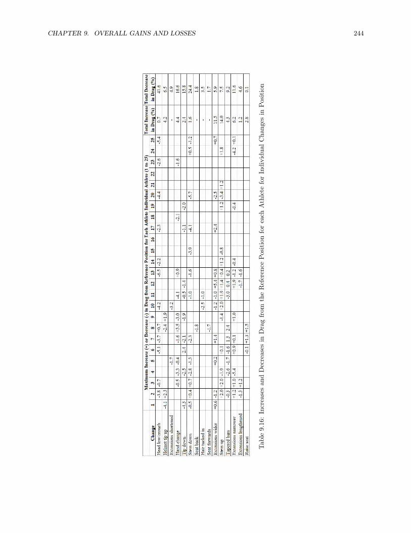
CHAPTER 9. OVERALL GAINS AND LOSSES 244
Tabl
e9.
16:
Incr
ease
san
dD
ecre
ases
inD
rag
from
the
Ref
eren
cePo
siti
onfo
rea
chA
thle
tefo
rIn
divi
dual
Cha
nges
inPo
siti
on

CHAPTER 9. OVERALL GAINS AND LOSSES 245
Tabl
e9.
17:
Incr
ease
san
dD
ecre
ases
inD
rag
from
the
Ref
eren
cePo
siti
onfo
rea
chA
thle
tefo
rM
ulti
ple
Cha
nges
inPo
siti
on

CHAPTER 9. OVERALL GAINS AND LOSSES 246
Tabl
e9.
18:
Incr
ease
san
dD
ecre
ases
inD
rag
from
the
Ref
eren
cePo
siti
onfo
rea
chA
thle
tefo
rE
quip
men
tC
hang
es*A
llw
heel
sw
ere
disc
whe
els.

CHAPTER 9. OVERALL GAINS AND LOSSES 247
The results in Figure 9.4 show that the majority of changes in position and equipment made during this studyreduced the aerodynamic drag, although this is not surprising as the overall aim of wind tunnel testing ofathletes is to optimise their position and reduce the drag. However, certain changes resulted in a significantincrease in drag, namely wearing a visor, raising the handlebar height, and widening the extensions. Byraising the handlebars and widening the extensions the frontal area will increase, and the trend betweenfrontal area and drag has already been identified as being significant. It is unclear why the addition of a visorhas shown to increase the drag, but a poor fit of the visor on the helmet and around the face of the athletemay be possible reasons for this increase. A further analysis of di!erent helmet and visor combinations ona number of athletes would be needed in order to validate this hypothesis. For changes to equipment, anincrease in drag was seen when modifications were made to the seat tube and stem, which suggests that thedesign of the competitive bike frame is already very aerodynamic. The greatest overall reductions in dragwere seen for a change in skinsuit, a change to the height and length of the extensions, and by adopting acrouch position. These changes in position help reduce the frontal area, and the material and seam placementof one of the skinsuits used for testing is likely to have been specifically designed to induce turbulence, delayseparation and reduce the skin friction drag in comparison to a standard, road skinsuit.
Another noticeable result from this study is the reduction in drag for all athletes when wearing shoe coverscompared to not wearing shoe covers. Although the influence of the actual shoe on the aerodynamic dragwas not tested in this study, all athletes wore their own shoes, which di!ered in shape, size and design. Asthe presence of a shoe cover reduced the drag for all athletes tested, this implies that the design of the shoeitself is not as important in terms of athlete performance as ensuring the athlete wears a shoe cover thateliminates seams, buckles and recesses from the oncoming flow.
The changes made to athlete position and to equipment can be ranked in order of their impact on aerodynamicdrag using the results described in this chapter, as shown in Table 9.19. These results show that multiplechanges in position have the most impact on aerodynamic drag, and therefore coaches should ensure thatathletes are in the most aerodynamic position as possible, specifically concentrating on lowering the stem andhead position to reduce the frontal area, before making changes to equipment in order to maximise athleteperformance.
Rank Change Average change in dragfrom reference position (%)
1 Multiple change in position 9.42 Skinsuit 6.33 Individual change in position 3.54 Frame and wheel combination 3.05 Helmet type 2.96 Visor vs no visor 2.27 Pedal/strap combination 2.18 Shoe Covers 1.89 Gloves vs no gloves 1.3
Table 9.19: Rank of factors in order of most influential on aerodynamic drag

CHAPTER 9. OVERALL GAINS AND LOSSES 248
Summary
This chapter has provided an insight into the overall gains and losses from changes in position and/orequipment, and attempted to rank these gains and losses in terms of their impact on the aerodynamic dragof a cyclist. The results have shown that the greatest reductions in drag came from obtaining a crouchedposition, wearing a di!erent skinsuit, and changing the extension height and length, but there was a widerange between the smallest and greatest di!erence in drag from the reference position between athletes, mainlydue to di!erences in body size and shape, riding experience, and reference position from which the changeswere made. However, certain changes in position and equipment resulted in having a significant impact onthe drag of all athletes tested (>1% gain or loss). Changes to the position of a cyclist a!ect the frontalarea and the flow over the rest of the body, which has shown to have a strong influence on the aerodynamicdrag. By bringing the handlebars down and lowering the head the aerodynamic drag was reduced for themajority of athletes, although actual percentage gains and the actual optimal set up varied between athletes.In general, multiple changes in position resulted in a greater impact on drag compared to individual changes,but changes were not additive. The reduction in drag by wearing shoe covers for all athletes tested, regardlessof shoe, pedal or cleat used, suggests that the design of the shoe itself is not as important as ensuring athleteswear a shoe cover that eliminates seams, buckles and recesses from the oncoming flow. The results suggestedthat elite riders were already in a fairly aerodynamic reference position, so smaller gains were identified forsome changes in position than were expected. Nevertheless this chapter has shown that changes to positionand equipment can be ranked in order of their influence on the aerodynamic drag, which can assist athletesand coaches with identifying those areas to focus on in order to maximise the speed of a cyclist and improveathlete performance.

Chapter 10
Conclusions
Introduction
A summary of the work and final conclusions are provided in this chapter. The original aims and objectivesare referred back to, and at the end of this chapter possible future research in this area is discussed.
10.1 Summary of Research
The aim of this research was to identify ways in which the velocity of a track cyclist could be maximised,and which factors had the greatest impact on the performance of all athletes involved by gaining a greaterunderstanding of the aerodynamics of cycling and the flow around a cyclist. As elite races are often won bymilliseconds, even small gains are significant and can result in a di!erence between an Olympic medal andno medal.
10.1.1 Objective 1: Appropriate Test Methods
The primary objective of this thesis was to develop appropriate test methods using the wind tunnel to measurethe aerodynamic drag and drag area of a cyclist, in order to make comparisons between changes in positionand/or equipment.
This aim was achieved by developing a cycle rig with a fixed and floating platform and a 50kg load cell tomeasure the drag for pedalling cyclists in the boundary layer wind tunnel at a wind speed of up to 46kph. Thefrontal area of the cyclist was measured using the digitising method, and a white board was used to projectthe shadow of the cyclist from side, which proved to be a successful method for monitoring athlete positionduring tests. The uncertainty of the force balance (±2.5%), wind speed (±0.13%), air density (±0.4%) andfrontal area (±2.5%) all propagate to the calculation of the drag coe"cient, resulting in a total error forthe drag coe"cient of ±2.6%. The boundary layer of the cycle rig was calculated to increase from 45mm to70mm, but all changes to position and/or equipment were made above the boundary layer and within thecore flow, so any e!ects of the boundary layer on the aerodynamic drag could be ignored.
249

CHAPTER 10. CONCLUSIONS 250
The simple model of a cyclist consisting of cylindrical arms, thighs and calves enabled an analysis to becarried out on the drag of material samples for the development of a new skinsuit for track cycling. Three,circular cylinders with rounded heads at the leading edge and diameters similar to the forearm, upper armand thigh of a cyclist were manufactured, and the aerodynamic drag measured for di!erent material samplesin the spanwise and streamwise orientations at 50kph to 80kph. The influence of the seam placement on thedrag was also measured for the spanwise cylinders. The accuracy of the material tests was dependent on thespeed, orientation and diameter of the cylinders; the smallest inaccuracy of 0.9% was for the large cylinderin the spanwise orientation at the highest speed, but the largest inaccuracy of 13% was for the small cylinderin the streamwise orientation at the lowest speed. However, the actual error of the drag readings was only±0.002kg. The results from the comparison of di!erent material samples and seam placement on the circularcylinders in di!erent orientations lead to the development of a prototype skinsuit, which was then comparedto the best existing New Zealand skinsuit by using a pedalling athlete on the cycle rig in the wind tunnel.Although the overall aerodynamic drag was similar for these two skinsuits, the results were promising for aninitial prototype.
10.1.2 Objective 2: Mathematical Model
The secondary objective of this thesis was to generate a mathematical model for track cycling that could beused to predict the velocity profile and finishing time for pursuit athletes, as well as to identify the optimalpacing strategy for pursuit cyclists.
This objective was achieved by using first principles to analyse the forces acting on a cyclist, leading tothe formation of equations for the power demand and power supply of cycling. The demand side equationsincluded the power to overcome drag, tyre and bearing rolling resistance, and weight, and the supply sideequations included the power produced by the athlete taken from actual SRM power data collected during aspecific race. It was assumed that any surplus power lead to acceleration of the system. This mathematicalmodel included the e!ect of leaning in the bends, something that most previous models had excluded. Thecalculation was performed in Microsoft Excel, firstly by calculating the initial acceleration and then usingthis result to determine the change in velocity over a specific timestep. The change in velocity was thenused to calculate the initial velocity for the next timestep, as well as the distance of the centre of mass andwheels over that timestep. This process was continued until the final distance was reached, at which pointthe finishing time could be identified. This method also allowed the velocity profile to be determined, whichclearly indicated the di!erence between the speed of the centre of mass of a cyclist in the bends comparedto the straights. The model was validated using SRM power data for eleven, pursuit, track cyclists, and theaverage accuracy of the model was shown to be 0.31s (0.16%). The greatest di!erence between the actualSRM data and the mathematical model was found to occur during the first lap, where the model wouldunderpredict the lap time. This was probably due to the increased drag area during the standing start inreality, which was not accounted for in the model. The model also underpredicted the velocity profile in boththe bends and straights by approximately 0.2ms!1, but nevertheless the model clearly proved to be able topredict the finishing time of IP athletes to a high degree of accuracy.
The model was successfully used to predict the di!erence in finishing times and velocity profiles for changesmade to the athlete, bike, and environmental conditions, the results of which indicated that the drag area,CdA, and the air density had the greatest influence on the finishing time. The model was also used tocompare the finishing times for di!erent pacing strategies whilst maintaining the same overall work done.

CHAPTER 10. CONCLUSIONS 251
The results suggested that an all-out strategy for 12s followed by an even or variable power output resultedin the fastest finishing time for a male, IP athlete (height of 1.85m, weight of 75kg, drag area of 0.195m2,and coe"cient of rolling resistance of 0.002) completing 4000m with a fixed stock of energy whose e"ciencyis not a function of power output or speed. An all-out and even or all-out and variable strategy resulted ina significantly faster finishing time than any other pacing strategy simulated for the 4000m IP, and lengthof time spent in the initial acceleration phase appeared to have a significant e!ect on the predicted finishingtime.
10.1.3 Objective 3: Most Significant Factors on Athlete Performance
The final objective of this thesis was to compare changes made in the wind tunnel to athlete position andequipment to identify those factors with the greatest impact on drag, to provide a rank of importance, andto identify the most significant ways in which the drag can be reduced.
This objective was achieved by using elite and competitive cyclists to compare changes in equipment, attireand position in the wind tunnel, and measuring the change in drag from the reference position for all changesmade. The reference position was chosen as the starting point from which changes were made because allathletes use di!erent equipment and adopt di!erent reference positions when riding to begin with, and thiswas agreed to be the most repeatable method to gain relative data for all athletes. By limiting the athletesto being at competitive or elite level, it was assumed that their reference position would already be fairlyaerodynamic and the results could therefore be comparable; recreational riders are likely to have a lessaerodynamic reference position, from which great gains would be seen by just changing to a position whichis similar to the reference position of an elite rider.
The changes made included frame and wheel combinations, modifications to the frame, di!erent types ofhelmets, helmets with and without a visor, pedal and strap combinations, gloves and no gloves, di!erentskinsuits, hand position, handlebar width and height, athlete torso and shoulder angle, and some generalchanges such as crouching, helmet tip position, seat position, and tucking the hair into the helmet or ina bun. The impact on drag was determined for each change made to the position and equipment, whichincluded both gains and losses from the reference position of each athlete. The average di!erence in drag foreach change was determined, which allowed the results to be ranked in order of greatest to least impact onthe overall drag of a cyclist. The mathematical model was also used to provide an estimate of time savingsor time gains for each change in position and equipment for a pursuit cyclist.
It was found that multiple positional changes had a greater impact on drag compared to individual postionalchanges, but changes were not additive, and a change in skinsuit had the greatest impact on drag out ofall equipment changes. A low handlebar position and a crouched or low head position resulted in a lowerdrag for most athletes, but it was not always the case that the lowest position was the best. Most positionalchanges were athlete dependent; not all athletes experienced the same gain or loss in drag for the samepositional change due to di!erences in body size and shape, riding experience, and reference position fromwhich the changes were made. However, the results did indicate that some changes in position had an impactof ±1% in drag for all athletes tested, which was considered to be a significant change for all track cyclists.A comparison of di!erent shoe covers concluded that the aerodynamic drag can be reduced by wearing shoecovers regardless of shoe, strap, pedal and cleat, which indicates that the design of the shoe itself may notbe as important as ensuring athletes wear a shoe cover. Although smaller gains in drag were seen for elite

CHAPTER 10. CONCLUSIONS 252
riders in general, probably due to their more aerodynamic reference position compared to competitive riders,the method of ranking changes from an athlete’s reference position showed to be a useful way to highlightwhere significant gains or losses can be made to the majority of athletes, which is beneficial to both coachesand athletes when deciding where to focus time, e!ort and money.
10.2 Conclusions
• Wind tunnel testing is an accurate method for measuring the aerodynamic drag of a cyclist, and canbe used successfully to compare changes in position and/or equipment;
• Mathematical models for track cycling should incorporate a factor for leaning in the bends in order toaccount for the di!erence in velocity of the centre of mass in the bends compared to the straights. Bygenerating supply and demand equations using first principles, an accurate model for track cycling canbe produced;
• Assuming a fixed work output of 128.3kJ, an all-out strategy for 12s followed by even or variable poweroutput (with a higher power in the bends compared to the straights) resulted in the fastest finishingtime for a male, IP athlete (height of 1.85m, weight of 75kg, drag area of 0.195m2, and coe"cientof rolling resistance of 0.002) completing 4000m with a fixed stock of energy whose e"ciency is not afunction of power output or speed. The time spent in the initial acceleration phase also had a significantinfluence on the finishing time;
• The drag area and air density have the greatest impact on the finishing time for pursuit cyclists;
• Multiple changes in athlete position have the greatest impact on the aerodynamic drag of a cyclist, butthe actual gains and losses seen by individual athletes will di!er due to di!erences in body size andshape, riding experience, and reference position from which changes were made;
• A low handlebar position and low head position reduces the frontal area of a cyclist, reducing the overalldrag by an average of 2% and 3.5% respectively. However, the lowest position is not necessarily themost aerodynamic position for all athletes;
• Changes to the skinsuit have the greatest impact on drag out of all equipment changes (an averagechange in drag of 6.3%), primarily due to the choice of material and seam placement, but the optimalmaterial and seam placement is dependent on the diameter and orientation of the cylindrical limbs, aswell as the cycling speed.
• Time savings of as much as 8 seconds over 4000m can be achieved through changes in position, and asmuch as 5 seconds over 4000m achieved through changes to the skinsuit (+/- 2%);
• In order to maximise the velocity of a cyclist athletes and coaches should concentrate on optimisingathlete position, primarily by lowering the handlebars and bringing the head into a more crouchedposition, followed by optimising equipment, in particular the skinsuit. However, individual testing isneeded in order to identify the optimal position for each athlete, due to the wide variablility betweenathlete body shapes and sizes, riding experience, and available equipment.

CHAPTER 10. CONCLUSIONS 253
10.3 Future Work
This study has highlighted the benefits of using wind tunnel tests to help reduce the aerodynamic drag ofcyclists through changes in position and equipment. At present there is limited research on the aerodynamicsof drafting cyclists using wind tunnel tests, especially for track cyclists. Although it is well known thatdrafting cyclists do not need to produce as much power as leading cyclists in order to maintain the samespeed, it is unclear of the true e!ects of spacing between athletes, the optimal order of team pursuit cyclists,the optimal position of each team pursuit rider, or the optimal changeover path. The e!ect of body size andshape on leading and drafting cyclists is not well understood, and these factors may have a significant e!ecton the performance of a team pursuit. A mathematical model of a team pursuit would also be a useful toolto identify the best order of team pursuit cyclists and how the position and spacing of each athlete a!ectsthe performance of the whole team. Although a few mathematical models do exist for drafting riders, thesemodels use only average power and velocity data for the entire team and it is not possible to analyse thee!ects of individual athletes on team performance.
In terms of optimal pacing strategy, it would be beneficial to generate di!erent scenarios for two di!erentathletes adopting the same pacing strategy, as well as for di!erent combinations of pacing strategies toidentify the outcome when two athletes compete against each other. A better understanding and preferablya quantitative model of the e!ects of fatigue and athlete psychology on the total work output of the rider isnecessary in order to model di!erent pacing strategies for conditions where the energy supplied by the athleteis not necessarily fixed, as it may be the case that athlete e"ciency is a function of power output or speed.
This thesis has concentrated on pursuit events for track cycling, but the principles of aerodynamics usedfor this study are applicable to all other cycling events as well as to other sports. Track cycling however,does exclude the e!ects of yaw angle, as it is assumed that there is no external wind present on an indoorvelodrome. For road cycling the e!ects of wind cannot be ignored.
A further study on the optimal position and type of aero helmet used for track cycling for di!erent athleteswould be very beneficial, in particular to understand the e!ect of vent location, size and shape on theaerodynamic drag. This thesis did not include a specific study on helmets, but only explored the di!erencein drag for riders comparing di!erent types of helmets. It would be useful to understand if there is a specifichelmet tip location that results in a low drag for all athletes wearing any type of helmet, or whether theposition of the helmet tip is dependent on the type of helmet as well as the size and shape of the athlete.
The e!ect of training was not part of this thesis, but experimental studies showed that certain positions, inparticular the arrow style hand position, caused riders to feel unstable. Therefore it would be beneficial toanalyse the e!ect of training on power output and stability of elite cyclists to determine whether athletesare able to train in a specific position in order to maximise their power output whilst minimising their drag.The experimental results for the optimal torso and shoulder angle for track cyclists indicated that maximumpower and minimum drag occurred at di!erent torso and shoulder angles, and that the shoulder angle hada greater influence on the power output of cyclists whereas the torso angle had a greater influence on theaerodyanmic drag. However, if athletes are able to train in a position that results in a lower drag in orderto maximise their power output, then it would not matter that their power output would initially be low inthis position.
As a closing remark, the significance of aerodynamics in gaining a competitive advantage in cycling is clear,

CHAPTER 10. CONCLUSIONS 254
and it is worth investing time and money in research and technology to find new ways to reduce the aerody-namic drag and maximise the speed of a cyclist.

Bibliography
C. R. Abbiss and P. B. Laursen. Describing and understanding pacing strategies during athletic competition.Sports Medicine, 38(3):239, 2008.
E. Achenbach. Influence of surface roughness on the cross-flow around a circular cylinder. Journal of FluidMechanics, 46(2):321–335, 1971.
E. Achenbach. Experiments on the flow past spheres at very high reynolds numbers. Journal of FluidMechanics, 54:565–575, 1972.
F. Alam, R. Brooy, A. Subic, and S. Watkins. Aerodynamics of cricket ball-an e!ect of seams (p70). TheEngineering of Sport 7, pages 345–352, 2008a.
F. Alam, A. Subic, A. Akbarzadeh, M. Estivalet, and P. Brisson. Aerodynamics of bicycle helmets. TheEngineering of Sport 7, pages 337–344, 2008b.
Bicycle Apparel. http://bicycleapparel.com/fabric.html, 2012.
G. Atkinson, R. Davison, A. Jeukendrup, and L. Passfield. Science and cycling: current knowledge and futuredirections for research. Journal of Sports Sciences, 21(9):767–787, 2003.
G. Atkinson, O. Peacock, and L. Passfield. Variable versus constant power strategies during cycling time-trials: Prediction of time savings using an up-to-date mathematical model. Journal of Sports Sciences, 25(9):1001–1009, 2007.
A.D. Auteuil, G.L. Larose, and S.J. Zan. Relevance of similitude parameters for drag reduction in sportaerodynamics. The Engineering of Sport 8, 2(2):2393–2398, 2010.
J. Baker, J. Gal, B. Davies, D. Bailey, and R. Morgan. Power output of legs during high intensity cycleergometry: influence of hand grip. Journal of Science and Medicine in Sport, 4(1):10–18, 2001.
C. Barelle, V. Chabroux, and D. Favier. Modeling of the time trial cyclist projected frontal area incorporatinganthropometric, postural and helmet characteristics. Sports Engineering, pages 1–8, 2010.
D. R. Bassett Jr, C. R. Kyle, L. Passfield, J. P. Broker, and E. R. Burke. Comparing cycling world hourrecords, 1967-1996: modeling with empirical data. Medicine and Science in Sports and Exercise, 31(11):1665, 1999.
B. S. Baum and L. Li. Lower extremity muscle activities during cycling are influenced by load and frequency.Journal of Electromyography and Kinesiology, 13(2):181–190, 2003.
255

BIBLIOGRAPHY 256
P. W. Bearman and J. K. Harvey. Control of circular cylinder flow by the use of dimples. AIAA journal, 31(10):1753–1756, 1993.
N. Belluye and M. Cid. Approche biomécanique du cyclisme moderne, données de la littérature: Biomechanicsapproach to modern cycling, literature data’s. Science and Sports, 16(2):71–87, 2001.
K. B. Blair and S. Sidelko. Aerodynamic performance of cycling time trial helmets (p76). The Engineeringof Sport 7, pages 371–377, 2008.
E. Bressel and J. Cronin. Bicycle seat interface pressure: reliability, validity, and influence of hand positionand workload. Journal of biomechanics, 38(6):1325–1331, 2005.
J. P. Broker. Cycling Power: Road and Mountain, chapter 6, pages 147–174. Human Kinetics, 2 edition,2003.
J. P. Broker, C. R. Kyle, and E. R. Burke. Racing cyclist power requirements in the 4000-m individual andteam pursuits. Medicine and Science in Sports and Exercise, 31(11):1677, 1999.
L. Brownlie, C. Kyle, J. Carbo, N. Demarest, E. Harber, R. MacDonald, and M. Nordstrom. Streamliningthe time trial apparel of cyclists: the nike swift spin project. Sports Technology, 2, 2009.
L. Brownlie, P. Ostafichuk, E. Tews, H. Muller, E. Briggs, and K. Franks. The wind averaged aerodynamicdrag of competitive cycling time trial helmets. 8th Conference of the International Sports EngineeringAssociation, 2(1):2419–2424, 2010.
L. W. Brownlie, I. Gartshore, A. Chapman, and E. W. Banister. The aerodynamics of cycling apparel.Cycling Science, 3(3-4):44–50, 1991.
E.R. Burke and A.L. Pruitt. Body Positioning for Cycling, chapter 3, pages 69–92. Human Kinetics, 2edition, 2003.
R. B. Candau, F. Grappe, M. MÉNard, B. Barbier, G. Y. Millet, M. D. Ho!man, A. R. Belli, and J. D.Rouillon. Simplified deceleration method for assessment of resistive forces in cycling. Medicine and Sciencein Sports and Exercise, 31(10):1441, 1999.
V. Chabroux, M. N. Mba, P. Sainton, and D. Favier. Wake characteristics of time trial helmets using piv-3ctechnique. In 15th International Symposium to Laser Techniques to Fluid Mechanics, 2010.
S. S. Chaudhari, R. S. Chitnis, and R. Ramkrishnan. Waterproof breathable active sports wear fabrics.Man-made Textiles in India, 5:166–171, 2004.
J Choi, WP Jeon, and H Choi. Mechanism of drag reduction by dimples on a sphere. Physics of Fluids, 18(4), 2006.
H. Chowdhury, F. Alam, and A. Subic. Aerodynamic performance evaluation of sports textile. The Engi-neering of Sport 8, 2(2):2517–2522, 2010.
K. R. Cooper, E. Mercker, and J. Wiedemann. Improved blockage corrections for blu! bodies in closed andopen wind tunnels, pages 1627–1634. Balkema, Rotterdam, 1999.
N. P. Craig and K. I. Norton. Characteristics of track cycling. Sports Medicine, 31(7):457, 2001.

BIBLIOGRAPHY 257
N. P. Craig, K. I. Norton, P. C. Bourdon, S. M. Woolford, T. Stanef, B. Squires, T. S. Olds, R. A. J. Conyers,and C. B. V. Walsh. Aerobic and anaerobic indices contributing to track endurance cycling performance.European Journal of Applied Physiology, 67(1):150–158, 1993.
R. S. Davis. Equation for the determination of the density of moist air(1981/91). Metrologia, 29(1):67–70,1992.
J. J. De Koning, M. F. Bobbert, and C. Foster. Determination of optimal pacing strategy in track cyclingwith an energy flow model. Journal of Science and Medicine in Sport, 2(3):266–277, 1999.
P. Debraux, W. Bertucci, A. V. Manolova, S. Rogier, and A. Lodini. New method to estimate the cyclingfrontal area. International journal of sports medicine, 2009.
T. Defraeye, B. Blocken, E. Koninckx, P. Hespel, and J. Carmeliet. Aerodynamic study of di!erent cyclistpositions: Cfd analysis and full-scale wind-tunnel tests. Journal of biomechanics, 43(7):1262–1268, 2010.
T. Defraeye, B. Blocken, E. Koninckx, P. Hespel, and J. Carmeliet. Computational fluid dynamics analysisof drag and convective heat transfer of individual body segments for di!erent cyclist positions. Journal ofbiomechanics, 44(1):1695–1701, 2011.
P. E. Di Prampero. The concept of critical velocity: a brief analysis. European journal of applied physiologyand occupational physiology, 80(2):162–164, 1999.
P. E. Di Prampero. Cycling on earth, in space, on the moon. European Journal of Applied Physiology, 82(5):345–360, 2000.
P. E. Di Prampero, G. Cortili, P. Mognoni, and F. Saibene. Equation of motion of a cyclist. Journal ofApplied Physiology, 47(1):201, 1979.
R. Drillis, R. Contini, and M. Bluestein. Body segment parameters: A survey of measurement techniques.In Selected articles from artificial limbs, Huntington, NY: Rovert E. Krieger Publishing Co. Inc.:329–351,1964.
A. G. Edwards and W. C. Byrnes. Aerodynamic characteristics as determinants of the drafting e!ect incycling. Medicine and Science in Sports and Exercise, 39(1):170, 2007.
Eschler. http://www.eschler.com/english/ecs/ecs.html, 2012.
E. W. Faria, D. L. Parker, and I. E. Faria. The science of cycling: Factors a!ecting performance-part 2.Sports Medicine, 35(4):313, 2005.
C. Foster, J. J. De Koning, F. Hettinga, J. Lampen, K. L. La Clair, C. Dodge, M. Bobbert, and J. P. Porcari.Pattern of energy expenditure during simulated competition. Medicine and Science in Sports and Exercise,35(5):826, 2003.
J. Garcia-Lopez, J. A. Rodriguez-Marroyo, C. E. Juneau, J. Peleteiro, A. C. Martinez, and J. G. Villa.Reference values and improvement of aerodynamic drag in professional cyclists. J Sports Sci, 1:10, 2008.
A.S. Gardner, P. Barratt, A. Wylie, C. White, D. Locke, M. Hughes, and J. Martin. Relative rider size doesnot influence drag reductions during velodrome cycling: 948: May 29. Medicine and Science in Sport andExercise, 41(5):129, 2009.

BIBLIOGRAPHY 258
G. Gibertini, G. Campanardi, D. Grassi, and C. Macchi. Aerodynamics of biker position. In BBAA VIInternational Colloquium on: Blu! Bodies Aerodynamics and Applications, 2008. Proceedings of theBBAA VI International Colloquium on: Blu! Bodies Aerodynamics and Applications.
G. Gibertini, D. Grassi, C. Macchi, and G. De Bortoli. Cycling shoe aerodynamics. Sports Engineering, 12(3):155–161, 2010.
M.N. Godo, D. Corson, and S.M. Legensky. An aerodynamic study of bicycle wheel performance usingcfd. American Institute of Aeronautics and Astronautics, 47th AIAA Aerospace Sciences Meeting(1):1–18,2009.
C. González-Haro, P. A. Galilea Ballarini, M. Soria, F. Drobnic, and J. F. Escanero. Comparison of nine the-oretical models for estimating the mechanical power output in cycling. British Journal of Sports Medicine,41:506–509, 2007.
F. Grappe, R. Candau, A. Belli, and J. D. Rouillon. Aerodynamic drag in field cycling with special referenceto the obree s position. Ergonomics, 40(12):1299–1311, 1997.
D. Greenwell, N. Wood, E. Bridge, and R. Addy. Aerodynamic characteristics of low-drag bicycle wheels.Aeronautical Journal, 99(983):109–120, 1995.
G. D. E. Groot, A. Sargeant, and J. O. S. Geysel. Air friction and rolling resistance during cycling. Medicineand Science in Sports and Exercise, 27(7):1090, 1995.
S.J Haake, S.R Goodwill, and M.J Carre. A new measure of roughness for defining the aerodynamics of sportsballs. Proceedings of the Institution of Mechanical Engineers Part C - Journal of Mechanical EngineeringScience, 221(7):789–806, 2007.
J. Hamill and E.C. Hardin. Special topics in biomechanics. In Foundations of Exercise Science, Ed. Kaman,G., 1st Ed.(Lippincott Williams and Wilkins):187, 2001.
F. J. Hettinga, Josj De Koning, F. T. Broersen, P. Van Ge!en, and C. Foster. Pacing strategy and theoccurrence of fatigue in 4000-m cycling time trials. Medicine and Science in Sports and Exercise, 38(8):1484, 2006.
S.F. Hoerner. Fluid-Dynamic Drag. 1965.
M. Hopkins, F. Principe, and K. Kelleher. Beyond materials: Du pont’s aerodynamic bicycle wheel. AdvancedMaterials: the Challenge for the Next Decade, 1(170):947–959, 1990.
A.F Huber II and T.J Mueller. The e!ect of trip wire roughtness on the performance of the wortmann fx63-137 aurfoil at low reynolds numbers. Experiments in Fluids, 5:263–272, 1987.
K Hyun Paul and S Kwang. The criterion of separation of incompressible laminar boundary layer flow overan axially symmetric body. Journal of the Franklin Institute, 325(4):419–433, 1988.
A Iniguez-de-la Torre and J Iniguez. Aerodynamics of a cycling team in a time trial: does the cyclist at thefront benefit? European Journal of Physics, pages 1365–1369, 2009.
K Jensen, L Johansen, and NH Secher. Influence of body mass on maximal oxygen uptake: e!ect of samplesize. European Journal of Applied Physiology, 84:201–205, 2001.

BIBLIOGRAPHY 259
S Jeon, J Choi, WP Jeon, H Choi, and J Park. Active control of flow over a sphere for drag reduction atsubcritical reynolds number. Journal of Fluid Mechanics, 517:113–129, 2004.
M. Jermy, J. Moore, and M. Bloomfield. Translational and rotational aerodynamic drag of composite con-struction bicycle wheels. Proceedings of the Institution of Mechanical Engineers, Part P: Journal of SportsEngineering and Technology, 222(2):91–102, 2008.
A. E. Jeukendrup and J. Martin. Improving cycling performance: how should we spend our time and money.Sports Medicine, 31(7):559, 2001.
A. E. Jeukendrup, N. P. Craig, and J. A. Hawley. The bioenergetics of world class cycling. Journal of Scienceand Medicine in Sport, 3(4):414–433, 2000.
G. H. Kuper and E. Sterken. Do skin suits a!ect the average skating speed? Sports Technology, 1, 2008.
C. R. Kyle and D. R. Bassett Jr. The Cycling World Hour Record, chapter 7, pages 175–196. Human Kinetics,2 edition, 2003b.
C. R. Kyle and M. D. Weaver. Aerodynamics of human-powered vehicles. Proceedings of the Institution ofMechanical Engineers, Part A: Journal of Power and Energy, 218(3):141–154, 2004.
C.R. Kyle. Selecting Cycling Equipment, chapter 1, pages 1–48. Human Kinetics, 2 edition, 2003a.
J.C Lin. Review of research on low-profile vortex generators to control boundary-layer separation. Progressin Aerospace Sciences, 38:389–420, 2002.
R Lukes, M Carre, and S Haake. Track Cycling: An Analytical Model, volume 1, pages 115–120. Springer,2006.
R. A. Lukes, S. B. Chin, and S. J. Haake. The understanding and development of cycling aerodynamics.Sports Engineering, 8(2):59–74, 2005.
J. C. Martin and N. A. T. Brown. Joint-specific power production and fatigue during maximal cycling.Journal of biomechanics, 42(4):474–479, 2009.
J. C. Martin, D. L. Milliken, J. E. Cobb, K. L. McFadden, and A. R. Coggan. Validation of a mathematicalmodel for road cycling power. Journal of Applied Biomechanics, 14:276–291, 1998.
J. C. Martin, A. S. Gardner, M. Barras, and D. T. Martin. Modeling sprint cycling using field-derivedparameters and forward integration. Medicine and Science in Sports and Exercise, 38(3):592, 2006.
J. C. Martin, C. J. Davidson, and E. R. Pardyjak. Understanding sprint-cycling performance: the integrationof muscle power, resistance, and modeling. International journal of sports physiology and performance, 2(1):5, 2007.
B. D. McLean and A. W. Parker. An anthropometric analysis of elite australian track cyclists. Journal ofSports Science, 7:247–255, 1989.
K. de Vey Mestdagh. Personal perspective: in search of an optimum cycling posture. Journal of AppliedErgonomics, 29(5):325–334, 1998.

BIBLIOGRAPHY 260
J.J. Miau, H.W. Tsai, Y.J. Lin, J.K. Tu, C.H. Fang, and M.C. Chen. Experiment on smooth, circularcylinders in cross-flow in the critical reynolds number regime. Exp Fluids, 51:949–967, 2011.
R. R. Neptune, C. P. McGowan, and J. M. Fiandt. The influence of muscle physiology and advancedtechnology on sports performance. Annual Review of Biomedical Engineering, 11:81–107, 2009.
L. Oggiano and L. Sætran. A low deag skinsuit for ski-cross competitions. The Engineering of Sport 8, 2(2):2387–2392, 2010.
L. Oggiano, L. Sætran, S. Løset, and R. Winther. Reducing the athletes aerodynamical resistance. Journalof Computational and Applied Mechanics, 5(2):1–8, 2006.
L. Oggiano, S. Leirdal, L. Sætran, and G. Ettema. Aerodynamic optimization and energy saving of cyclingpostures for international elite level cyclists (p114). The Engineering of Sport 7, pages 597–604, 2008.
L. Oggiano, O. Troynikov, I. Konopov, A. Subic, and F. Alam. Aerodynamic behaviour of single sport jerseyfabrics with di!erent roughness and cover factors. Sports Engineering, 12(1):1–12, 2009.
T Olds. The mathematics of breaking away and chasing in cycling. European journal of applied physiologyand occupational physiology, 77(6):492–497, 1998.
T. Olds. Modelling human locomotion. Sports Med, 31(7):497–509, 2001.
T. Olds and S. Olive. Methodological considerations in the determination of projected frontal area in cyclists.Journal of sports sciences, 17(4):335–345, 1999.
T. S. Olds, K. I. Norton, and N. P. Craig. Mathematical model of cycling performance. Journal of AppliedPhysiology, 75(2):730–737, 1993.
T. S. Olds, K. I. Norton, E. L. Lowe, S. Olive, F. Reay, and S. Ly. Modeling road-cycling performance.Journal of Applied Physiology, 78(4):1596, 1995.
J.C. Owen and P.W Bearman. Passive control of viv with drag reduction. Journal of Fluids and Structures,15:597–605, 2001.
Craig Palmer. Bikenz personal communication, 2009.
R. C. Pankhurst and D. W. Holder. Wind-tunnel technique: an account of experimental methods in low-andhigh-speed wind tunnels. Sir Isaac Pitman and Sons Ltd, 1952.
D. R. Pendergast, J. C. Mollendorf, R. Cuviello, and A. C. Termin. Application of theoretical principles toswimsuit drag reduction. Sports Engineering, 9(2):65–76, 2006.
Kathryn Phillips. Bikenz personal communication, 2011.
PropellerGuard. www.propellersafety.com/propeller-guard-reduced-drag/, 2011.
C. C. Raasch, F. E. Zajac, B. Ma, and W. S. Levine. Muscle coordination of maximum-speed pedaling.Journal of biomechanics, 30(6):595–602, 1997.
UCI Cycling Regulations. www.uci.ch„ 2009.
Andy Reid. Bikenz personal communication, 2012.

BIBLIOGRAPHY 261
S.K Roberts and M.I Yaras. Boundary-layer transition a!ected by surface roughness and free-stream turbu-lence. Journal of Fluids Engineering, 127:449–457, 2005.
S.K Roberts and M.I Yaras. E!ects of surface-roughness geometry on separation-bubble transition. Journalof Turbomachinery, 128:349–356, 2006.
N.R Rodriguez, N.M DiMarco, and S Langley. Nutrition and athletic performance. Med Sci Sports Exerc,41(3):709–731, 2009.
Roymech. www.roymech.co.uk, 2011.
David Salazar. A2 wind tunnel charlotte personal communication, 2011.
Hhcm Savelberg, I. G. L. Van de Port, and P. J. B. Willems. Body configuration in cycling a!ects musclerecruitment and movement pattern. JAB, 19:4, 2003.
H Schlichting. Boundary layer theory. McGraw-Hill Series in Mechanical Engineering, 7th edition, 1979.
Helen Searle. University of canterbury personal communication, 2012.
L. Seatran and L. Oggiano. Skin suit aerodynamics in speed skating. Sport Aerodynamics: CISM Coursesand Lectures, 506, 2008.
R. C. H. So, J. K. F. Ng, and G. Y. F. Ng. Muscle recruitment pattern in cycling: a review. Physical Therapyin Sport, 6(2):89–96, 2005.
D.P. Swain. A model for optimizing cycling performance by varying power on hills and in wind. Medicineand Science in Sports and Exercise, 29(8):1104, 1997.
J. Sznitman, F. Kritter, and T. Rosgen. Flow visualization of bicycle helmets for optimal ventilation design.Summer Heat Transfer Conference. San Francisco, 1(1):HT2005–72751, 2005.
M. Tapias, M. Rallo, J. Escofet, I. Algaba, and A. Riva. Objective measure of woven fabric’s cover factor byimage processing. Textile Research Journal, 80(1):35–44, 2010.
G. S. Tew and A. T. Sayers. Aerodynamics of yawed racing cycle wheels. Journal of Wind Engineering andIndustrial Aerodynamics, 82(1-3):209–222, 1999.
B. E. Thompson, W. A. Friess, and K. N. Knapp. Aerodynamics of speed skiers. Sports Engineering, 4(2):103–112, 2001.
D Too and G.E Landwer. The biomechanics of force and power production in human powered vehicles.Human Power, 55:3–6, 2004.
M Torres. Technical soaring. The Soaring Society of America, 1999.
Weather Underground. www.wunderground.com, 2009.
S. G. J. van Ingen and P. R. Cavanagh. Power equations in endurance sports. Journal of biomechanics, 23(9):865, 1990.
F.M. White. Viscous Fluid Flow. McGraw-Hill, Inc., 2nd edition, 1991.

BIBLIOGRAPHY 262
R.L. Wilber. Altitude Training in Preparation for Competition at Sea Level, chapter 8, pages 197–240. HumanKinetics, 2 edition, 2003.
D.G. Wilson. Bicycling Science. The MIT Press, London, 3 edition, 2004.
Y. Yamagishi and M. Oki. E!ect of groove shape on flow characteristics around a circular cylinder withgrooves. Journal of Visualization, 7(3):209–216, 2004.
M. Zdravkovich, M. Ashcroft, S. Chisholm, and N. Hicks. E!ect of cyclist’s posture and vicinity of anothercyclist on aerodynamic drag. The Engineering of Sport 6, 1(1):21–28, 1996.
C Çengel and JM Cimbala. Fluid mechanics, fundamentals and applications. McGraw-Hill, 2006.

Appendix A
UCI Rules and Regulations
All equipment used on the track for world events must be approved by the UCI and must comply with thespecifications described in the Approval Protocols [Regulations, 2009]. These rules and regulations ensure allathletes compete on an equal level, but they also limit the options for changes to position and equipment.
Frames and Forks
A bicycle is defined as a vehicle which has two wheels of the same diameter: the front wheel steerable andthe rear wheel driven through a system comprising of chains and pedals (Rule 1.3.006). The bike must beavailable to all participants, and therefore must be marketed or for sale by the manufacturer. The bike mustcomply with all safety regulations and allow the rider to adopt the necessary position without di"culty orrisk. The bike must weigh a minimum of 6.8kg, excluding any additional accessories, such as an SRM PowerMeter. The minimum and maximum measurements for which the bike must comply with are shown in FigureA.1 and Table A.1.
Figure A.1: Bike Measurements
263

APPENDIX A. UCI RULES AND REGULATIONS 264
Measurement Minimum Maximum1.3.012 Bike overall dimensions - 185cm in length and 50cm in width1.3.013 Distance between the centre of the 5cm
bottom bracket axle and tip of the saddle1.3.014 Saddle length 24cm 30cm1.3.015 Distance between bottom bracket spindle and ground 24cm 30cm1.3.016 Distance between vertical passing through 54cm 65cm
bottom bracket spindle and front wheel spindle1.3.016 Distance between vertical passing through 35cm 50cm
bottom bracket spindle and rear wheel spindle1.3.017 Distance between internal extremities of front forks - 10.5cm1.3.017 Distance between internal extremities of rear triangle - 13.5cm1.3.018 Wheel diameter including tyres (for non mass start races) 55cm 70cm1.3.023 Distance between bottom bracket spindle and end of extensions* - 75cm
Table A.1: Bike Measurements*+5cm tolerance
The frame must be built around a main triangle and constucted from straight or tapered tubular elements.The cross section of the tubular elements may be round, oval, flattened, teardrop shaped or otherwise, so thatthe form of each element encloses a straight line, and they must be connected in a specific way [Regulations,2009, 1.3.020c]. The stem, handlebar, handlebar extension, and seat post elements must be a maximumheight of 8cm and minimum thickness of 2.5cm, as shown in Figure A.2, and must conform to a 3:1 ratio.Moving parts, pedals, front/rear derailleur mechanisms, wheel brake mechanisms and the saddle are exemptfrom this rule. The pedal crank is also exempt from this rule, but its transverse dimension is restricted to8cm. The minimum thickness may be reduced to 1cm for the chain stays and the seat stays. The minimumthickness of the front fork must be 1cm, and these may be straight or curved. For track competitions, theelements of the frame may be solid or tubular, assembled or cast in a single piece in any form. These elementsmust fit within the triangular form template.
Figure A.2: Shape of frame elements

APPENDIX A. UCI RULES AND REGULATIONS 265
It is prohibited to have any device to decrease air resistance or artificially accelerate propulsion, such asprotective screening, windscreens, or fuselage form fairing. A fuselage form shall be tolerated provided thatthe ratio between the length, L, and diameter, D, does not exceed 3 (see Figure A.3). Therefore the shape ofthe frame elements may similar to a tear drop, provided the length to diameter ratio is less than 3. Fairingsare also prohibited, and it should be possible to pass a rigid card, such as a credit card, between the fixedstructure and moving part.
Figure A.3: Length to diameter ratio
Only traditional handlebars are permitted for track races, with the exception of the IP, TP, and 500m TT,where the bike may be fitted with a handlebar extension upon which the forearm or elbow rests. The rider’sforearms must be in a horizontal plane and the extension designed so that the rider can adopt and maintaina regulatory position for the entire duration of the event. The profile of the extensions must also conform tothe 3:1 ratio, and the extensions must be fixed so that changes in length or angle are not possible during therace. The extensions only permit extension in the horizontal plane, and must be fitted with hand grips. Thehand grips may be horizontal, inclined or vertical, as shown in Figure A.4, but must be recognisable and onlybe used for hand contact. Extensions that are raised or arc-shaped are not permitted. Riders must have atleast one hand on the handlebars at all times.

APPENDIX A. UCI RULES AND REGULATIONS 266
Figure A.4: Handlebar extensions
Rider Position
The rider position for the pursuit races is defined by two measurements: (1) the position of the tip of thesaddle behind the bottom bracket (-5cm minimum), and (2) the advanced position using the extensions(+75cm maximum). Riders who consider that they cannot respect these regulations due to morphologicalreasons may request for an exemption from the regulations. This request only applies to either the saddleposition or the advanced handlebar position, not both.
Apparel
The rules state that when competing, athletes must wear a jersey with sleeves and shorts, possibly in theform of a skinsuit, where the shorts must come above the knee and sleeveless jerseys are not allowed. Inaddition, one must be able to distiguish between riders in the same team wearing the same clothing. For theIP, TP, 500m TT and 1km TT events the rider must wear one race number, but for all other events the ridermust wear two race numbers.

Appendix B
Existing Mathematical Models forCycling
DiPrampero et al. (1979)
P = (0.045MV ) + (0.041BSAPBT V 3)
where P is the power output (W), M is the mass of the cyclist (kg), V is the velocity of the system(m/s), PB is the barometric pressure (Torr), T is the temperature (K), BSA is the body surface area (m2).(BSA = 0.007184BM0.425Ht0.725),
/, BM is the mass of the cyclist (kg), Ht is the height of the cyclist (m).
Bassett Jr et al. (1999)
P = K(0.00953MtV + 0.00775V 2 +K1(Af )0.007551V 3)
where K is a factor which allows for adjustment for track roughness or other external conditions, K1 is anaerodynamic factor which incorporates a correction for altitude, rider position, bicycle type, components,clothing, helmets etc. (but not wind because the model is used for track cycling in a velodrome where thee!ect of wind is unpredictable), V is the cycling speed (ms!1), and Af is the frontal area of the system (m2)(Af = 0.0293H0.725M0.425 + 0.0604).
Candau et al. (1999)
P = CR ·M · g · (DRTR
) + !2 ·ACd · (DR
TR)3
where P is the mechanical power output (W), CR is the coe"cient of rolling resistance (0.00563), M is themass of the bike and rider (kg), g is the acceleration due to gravity (9.81ms!1), DR is the race distance (m),TR is the race time (s), " is the air density (1.22 kgm!3 at sea level), and ACd is the e!ective frontal area(0.333m2).
267

APPENDIX B. EXISTING MATHEMATICAL MODELS FOR CYCLING 268
Lukes et al. (2006)
ma = (- PrV )! (CdA
12"V
2)! ((mV 2
rmcos$+mgsin$)µRCs)
where m is the total mass of the system (kg), a is the acceleration (ms!2), - is the e"ciency factor, Pr
is the rider’s power, V is the bike velocity (ms!1), Cd is the drag coe"cient, A is the frontal area of thesystem (m2), " is the air density (kgm!3), rm is the radius of curvature of the centre of mass (m), g is theacceleration due to gravity (ms!2),$ is the tipping angle relative to the horizontal (°), µR is the coe"cientof rolling resistance, and Cs is the scrubbing correction coe"cient.
Martin et al. (1998)
PTOT =[V 2
a VG12!(CdA+FW )+VGCRRmT g+VG(91+8.7VG)10!3+VGmT gGR+ 1
2 (mT+ Ir2
)(V 2
Gf!V 2Gi)
(ti!tf ) ]
Ec
where Ec is the chain e"ciency factor (97.698%), Va is the air velocity (ms!1), VG is the ground velocity ofthe bike and rider (ms!1), Cd is the drag coe"cient, A is the frontal area of the system (m2), CRR is thecoe"cient of rolling resistance, mT is the total mass of the bike and rider (kg), g is the acceleration due togravity (ms!2), GR is the grade (rise/run), I is the moment of inertia of the 2 wheels (0.14kgm2), ti is theinitial time (s) and tf is the final time (s), and VGi is the initial ground velocity (ms!1) and VGf is the finalground velcity (ms!1).
Martin et al. (2006)
Power = (CdA" ( 12"V2a VG) + µ" (VgFN ) + $PE
!t + !KE$t )E
where Cd is the drag coe"cient, A is the frontal area of the rider, bike and wheel spokes, µ is the globalcoe"cient of friction (including Crr and bearing friction), E is the e"ciency of the drive system (assumedto be 97.7%), PE is potential energy, KE is kinetic energy, " is the air density, and FN is the normal forceexcerted by the bike on the rolling surface (essentially the weight of the bike and rider). CdA and µ are foundby regression analysis.
Olds et al. (1993)
ETOT = ERr + ERa + EG + Eacc
where ETOT is the total energy (J), ERr is the energy required to overcome rolling resistance (J), ERa is theenergy required to overcome air resistance (J), EG is the energy required to ride on a grade (J), and Eacc isthe energy required for acceleration (J).
ERr = CRrcos(arctanS)(M +Mb)d
where CRr = constant (coe"cient of rolling resistance = 0.0457), S is the slope (%), M is the mass of thecyclist (kg), Mb is the mass of the bike (kg), and d is the race distance (m).
ERa = 0.19 · CF! · CFA · (Vss + Vw)2 · (d! dacc)

APPENDIX B. EXISTING MATHEMATICAL MODELS FOR CYCLING 269
where CF! is the correction factor for air density, CFA is the correction factor for body surface area, Vss isthe steady state bike speed (m/s), Vw is the head wind speed (m/s), dacc is the distance required to achievethe final Vss (m).
CF! = (PB ·288)(755·T )
CFA = BSA1.77
BSA = M0.425Ht0.725 · 0.007184
where PB is the barametric pressure (mmHg), T is the ambient temperature (K), BSA is the body surfacearea (m2), M is the mass of the cyclist (kg), and Ht is the height of the cyclist (m).
EG = (M +Mb) · g · sin(arctanS) · d
Eacc = 0.5 · (M +Mb) · V 2ss + 0.19 · CF" · CFA · (V 2
w + (Vss + Vw)2) · (dacc2 )
Olds et al. (1995)
Demand = ERr + Eair + Egrade + EKE
where Demand is the energy demand of cycling (J), ERr is the energy required to overcome rolling resistance(J), Eair is the energy required to overcome air resistance (J), Egrade is the energy to move system vertically(J), EKE is the energy required to impart kinetic energy to the system (J).
ERr = d · µR · cos(arctanS) · CFgrav · 9.80665 · (M +Mb)
µR =(a+ b
P )Diam · CFsurface
CFgrav = ( 6.378(6.378+( Alt
1000 )))2
Egrade = d · (M +Mb) · CFgrav · 9.80665 · sin(arctanS)
where d is the race distance (m), µR is the coe"cient of rolling resistance, S is the slope (%), CFgrav is thefactor correcting the acceleration due to gravity for altitute, M is the nude mass of the rider (kg), Mb is themass of the bike and accessories, including clothing (kg), a=-0.00051, b=9.73744, P is the tyre pressure (psi),Diam is the diameter of the wheels (inches), CFsurface is the factor correcting µR for road surface (asphalt= 1, concrete = 0.87), and Alt is the altitude above sea level (m).
Eair = 0.5 · CFD · Cd ·Ap · " · CFxwind · Vss · (t+ 3k(!t/k) ! 1.5k(!2t/k) + (k3 )(!3t/k) ! 11k
6 ) +KEang
CFD = 1! 0.3835 + 1.25 · Spacing2
Ap = 0.4147 · ( Ab1.771 ) + 0.1159
Ab = Ht0.725·M0.425 · 0.007184
" = 1.225 · ( PB260 ) · (
288.15T ) · CFhumidity
CFhumidity = ( PO2·32+PN2·28+PH2O·180.2093·32·PB ·+0.7904·28·PB
)
PH2O = 15.573(0.0606·(T!291)) · (RH100 )
PO2 = 0.2093 · (PB ! PH2O)
PN2 = 0.7904 · (PB ! PH2O)

APPENDIX B. EXISTING MATHEMATICAL MODELS FOR CYCLING 270
CFxwind =,(V 2
ss + V 2w + 2 · Vss · VwcosXwind) · (Vss +
VwcosXwindV 2ss
)
where CFdraft is the factor correcting Eair for drafting, Cd is the drag coe"cient of the system (0.592), Ap
is the projected frontal area of the system (m2) (Ap = 0.3176 · 0.007184 · BM0.425 ·Ht0.725 ! 0.1478 whereBM is the mass of the cyclist (kg) and Ht is the height of the cyclist (m)), " is the air density (kg.m!3),CFXwind is the factor correcting air resistance for cross winds, Spacing is the distance between cyclist andpack/paceling/vehicle (m), Ab is the body surface area (m2), Ht is the height of the cyclist (cm), PB isthe barometric pressure (mmHg), T is the ambient temperature (K), CFhumidity is the factor correcting airdensity for humidity, PH2O is the partial pressure of water vapour (Torr), RH is the relative humidity (%),PO2 is the partial pressure of oxygen (Torr), PN2 is the partial pressure of nitrogen (Torr), Vss is the steadystate bike speed (ms!1), Vw is the wind speed (ms!1), Xwind is the angle of the wind relative to directionof travel of system (rad), t is the time (s), k is the time constant for acceleration (10) (s), and KEang is theangular kinetic energy.
EKE = 0.5 · (M +Mb) · (Vss · (1! exp(!t/k)))2 +KEang
where KEang= hip joint + knee joint + ankle joint + cranks/pedal + pedal + cluster + wheels + chainwheels
Hip joint = 0.3536 ·M · (0.39 · Ht170.18 · 0.785 · cad
60
Knee joint = 0.1286 ·M · (0.27 · Ht170.18 · 1.309 · cad
60
Ankle joint = 0.0276 ·M · (0.18 · Ht170.18 · 0.349 · cad
60
Cranks/pedal = 1.2 · 0.14 · cad · $30
Pedals = 0.45 · 0.03 · cad · $30
Cluster = 0.46 · 0.02 · Vss " (1!(!t/k))(Diam·0.0127)
Wheels = 3.16 · 0.23 · Vss " (1!(!t/k))(Diam·0.0127)
Chainwheels = 0.25 · 0.08 · cad · $30
where cad is the cadence (rpm)

Appendix C
Details of Simulated Pacing Strategies
Strategy Equation Parabolic Equation Linear Pbends Pstraights
All-out Phase Phase (W) (W)
All-out 10s & variable higher bends P = !17.76t2 + 177.6t + 600 507.5 407.5
All-out 12s & variable higher bends P = !12.33t2 + 148t + 600 504 404
All-out 14s & variable higher bends P = !9.0612t2 + 126.86t + 600 501 401
All-out 16s & variable higher bends P = !6.9375t2 + 111t + 600 497 397
All-out 18s & variable higher bends P = !5.48t2 + 98.67t + 600 493 393
All-out 10s & variable higher straights P = !17.76t2 + 177.6t + 600 438 538
All-out 12s & variable higher straights P = !12.33t2 + 148t + 600 435 535
All-out 14s & variable higher straights P = !9.0612t2 + 126.86t + 600 431.5 531.5
All-out 16s & variable higher straights P = !6.9375t2 + 111t + 600 427.5 527.5
All-out 18s & variable higher straights P = !5.48t2 + 98.67t + 600 424 524
All-out 10s even P = !17.76t2 + 177.6t + 600 473 even
All-out 12s even P = !12.33t2 + 148t + 600 470 even
All-out 14s even P = !9.0612t2 + 126.86t + 600 466 even
All-out 16s even P = !6.9375t2 + 111t + 600 452.5 even
All-out 18s even P = !5.48t2 + 98.67t + 600 458.5 even
Variable higher bends 515 415
Variable higher straights 449.5 549.5
All-out 10s linear decline P = !17.76t2 + 177.6t + 600 P = !0.93t ! 600 363 end
All-out 12s linear decline P = !12.33t2 + 148t + 600 P = !0.945t ! 601 360 end
All-out 14s linear decline P = !9.0612t2 + 126.86t + 600 P = !0.96t ! 602 358 end
All-out 16s linear decline P = !6.9375t2 + 111t + 600 P = !0.986t ! 603 354 end
All-out 18s linear decline P = !5.48t2 + 98.67t + 600 P = !t ! 604 353 end
Even 482.5 even
Positive 113% (527W) 101% (471W) 100% (466W)
Negative P = 0.458t ! 1137 466 even 695 end
U-shaped P = 0.00006d2 ! 0.233d + 631 135.5% (631W) 85.5% (398W) 135.5% (631W)
J-shaped P = 0.00002d2 ! 0.46d + 466 100% (466W) 95% (443W) 135% (629W)
Reverse J-shaped P = 0.00003d2 ! 0.141d + 607 130.3% (607W) 90.3% (421W) 100.3% (467W)
Table C.1: Details of Simulated Pacing Strategies
271

Appendix D
Wind Tunnel Testing Procedure
Images of LabVIEW displays
Figure D.1: LabVIEW front panel display
272

APPENDIX D. WIND TUNNEL TESTING PROCEDURE 273
Figure D.2: LabVIEW graph of data collection
Figure D.3: LabVIEW display for analysing data
Description of Testing Procedure
1. The floating platform is locked to prevent movement while the bike is placed in position on the rig andthe athlete gets on to the bike.

APPENDIX D. WIND TUNNEL TESTING PROCEDURE 274
2. The atmospheric temperature and pressure are recorded.
3. A camera is placed to the side of the athlete and behind the athlete to video athlete position duringeach test and to take still images.
4. After ensuring the rider is in their correct racing position, an outline of the rider is drawn on a whiteboard placed to the side of the athlete.
5. The system is calibrated by loading and unloading the 2kg weight using a syringe system.
6. The wind is turned on.
7. Once the wind is up to speed the athlete begins pedalling at a comfortable cadence for 30 seconds andthe data recorded. At the same time the cameras are turned on to take video and still images, and theathlete position with respect to the white board monitored.
8. After 30 seconds the athlete stops pedalling but remains in their racing position. It is possible for theathlete to pedal for longer than 30 seconds in order to gather data for a number of position changesduring the same test if this is desired. Labels can be made in the software to identify changes in positionduring the same test.
9. Once the wind has stopped completely the system is calibrated again by loading and unloading the 2kgweight using the syringe system, and the overall drift calculated by subtracting the initial calibrationvalue from the final calibration value.
10. The platform is then locked again so the athlete can get o! the bike, and the data then reloaded intoanother LabVIEW programme for analysis.
11. Moveable cursors on a graphical display of the drag data allow the average drag to be calculated foreach test. For tests where the athlete has changed position during the run, the average drag for eachposition can be determined in the same way, by selecting the corresponding regions on the graph withthe moveable cursors.
12. The data is imported into the Microsoft Excel spreadsheet shown in Figure D.4 to calculate the timegains for di!erent changes in position.

APPENDIX D. WIND TUNNEL TESTING PROCEDURE 275
Figure D.4: Calculation of Time Gain for Wind Tunnel Tests
13. The images taken from the rear of the rider during each test can be used to calculate the frontal areaof the rider in that position using the digitising method.

Appendix E
Changes for Overall Gains
Changes in Position
• Tucked head/crouch/head low - moving the head down, tucking the head in, but ensuring the cyclistscontinue to look forwards.
• Helmet tip up - lifting the tip of the helmet only, but ensuring the athletes can still look forwards.
• Extensions shortened - bringing the extensions closer to the body, but keeping them parallel.
• Hand change - changing the position of the hands on the extensions.
• Tip down - lowering the tip of the helmet so it is lower than the reference position, but not necessarilytouching the back of the rider.
• Stem down - moving the stem down to lower the front of the body.
• Seat backwards - moving the seat backwards, but maintaining the same height (this will also alter theleg extension of the rider).
• Hair tucked in - only for athletes with hair long enough to tie into a bun or secure under the helmet.
• Seat forwards - moving the seat forwards, but maintaining the same height (this will also alter the legextension of the rider).
• Extensions wider - keeping the extensions parallel, but moving them wider.
• Stem up - raising the stem to lift the handlebars.
• Tapered bars - maintaining the same hand position, but moving the elbows out by either widening theelbow pads or tilting the extensions.
• Extensions narrower - maintaining parallel extensions, but bringing them closer together.
• Extensions lengthened - moving the extensions further away from the body to lengthen the athlete.
• Raise seat - making the seat higher without changing the fore-aft position of the seat (this will alsoalter the leg extension).
276

APPENDIX E. CHANGES FOR OVERALL GAINS 277
Equipment Changes
• Di!erent skinsuit - comparison between road and track, competitive and recreational skinsuits.
• Di!erent frame and wheels - all wheels were disc wheels, but the frames were a combination of roadand track racing frames.
• Di!erent helmet - comparison between di!erent racing helmets, including aero helmets and non-aerohelmets.
• Same frame, di!erent wheels - changing the front and rear wheels (all disc wheels).
• No visor vs visor - removing the visor from the helmet.
• Pedal/strap combination - changing the type of pedals and straps used in sprint cycling.
• Shoe covers vs no shoe covers - covering the shoes and ankle socks with a shoe cover.
• Same pedal di!erent strap - changing the type of strap used in sprint cycling, but with the same pedalas the reference position.
• Gloves vs no gloves - wearing di!erent types of gloves while holding the same hand position on dropbars (cowhorn bars).
• Helmet holes taped vs untaped - taping over the vents of the helmet with electrical tape.
• Same strap di!erent pedal - changing the type of pedal used in sprint cycling, but with the same strapas the reference position.
• Modified seat tube - changing the shape of the seat tube by using polestyrene covered in electrical tapeto try and make a more streamlined shape.
• Modified fork shape - changing the shape of the front forks by using polestyrene covered in electricaltape to try and make a more streamlined shape.
• Modified stem shape - changing the shape of the stem by using polestyrene covered in electrical tapeto try and make a more streamlined shape.