AERODYNAMIC HEATING OF A SWEPT BACK WEDGE AIRFOIL

By

R • .. Pall1.0lgyi . .

Thesis submitted in partial fulfillment

of the requirements for the degree of

Master of Engineering

Department of Mechanical Engineering

McGill University

Montreal

Apri l 1961

- i -

SUMMARY

Aerodynamic heating of a swept

wedge airfoil was investigated i~ a Mach Number 2.58

flow for various sweep angles. The 2 in. x 1 1/4 in.

surface size airfoil was made of stainless steel with

a sharp leading edge and a wedge angle of 22. Q,,:qegrees.

The angle of attack in a plane normal to the leading edge

was constant at 5 degrees, the sweep angle varied from

0 to 35 degrees in five degree increments. Forty

chromel-alumel thermocouples were welded to one surface

of the wedge, in order to measure the temperature

distribution of the surface.

For every sweep angle the equilibrium

wedge surface temperature was calculated theoretically

and measured experimentally. Theoretical and experi­

mental results were found to be within a +lü% agreement.

Theoretical investigation indicated that sweep angle

had only negligible effect on aerodynamic heating.

- ii -

ACKNOWLEDGEMENTS

The author wishes to express appreciation

and thanks for the help and cooperation obtained with.

this work.

To Sannu Molder for his help in finding

reference works. To Bela Takats for doing the precise

and complicated welding work. To Jack Kelly for

controlling the operation of the main test facility.

To Seymour Epstein for taking charge of the electrical

equipment. To Miss Janine Lacroix for the typing of

the manuscript. Finally to the Canadian Defence

Research Board whose financial support made the work

possible.

,..

- iii -

CONTENTS

SUIVIIVIARY •••••••••••••••••••••••••••• o • • • • • • • • • • • i

ACKNOWLEDGEMENTS 0 0 0 0 0 0 0 0 0 0 0 G 0 0 0 0 0 0 0 0 0 0 0 0 0 0 0 0 0 0 0 ii

CONTENTS • • • • • • • • • • • • • • • • • • • • 0 0 • • • • • • • • 0 • • • • • • • • iii

LIST OF SYMBOLS • • • • • • • • • • • • • • • • • • • • • 0 • • • • • • • • 0 • v

INTRODUCTION ••••••••••••••••••••••••••••••••••• 1

HISTORICAL REVIEW

A. Historical Introduction •••••••••••••••• 3

B. Review on Boundary Layer Research Concerning Heat Transfer •••••.••••••••• 4

THEORETICA~ DISCUSSION

A. Basic Assumptions . . . . . . . . . . . . . . . . . . . . . . 8

B. Review of Oblique Shock Cbaracteristics. 8

I. Two dimensional oblique shock waves •••••••••••••••••••••••••••• 9

II. Effect of sweep on flow characteristics ••••••••••••••••• 11

c. Heat Transfer Between Air Stream and Surface . . . . . . . . . . . . . . . . . . . . . . . . . . . . . . . . 13

D. Effect of Sweep Angle on Aerodynamic Heating •••••••••••••••••••••••••••••••• 15

EXPERIMENTAL APPARATUS

A. The Main Test Facility . . . . . . . . . . . . . . . . . 19

B. Nozzle and Wedge • • • • • • • • • • • • • • • • • • • • • • • 19

c. Instrumentation • • • • • • • • 0 • • • • • • • • • • • • • 0 • 20

TEST PROCEDURE

A. Operation Technique . . . . . . . . . . . . . . . . . . . . 22

B. Calibration of the Nozzle . . . . . . . . . . . . . . 22

C. Measurements . . . . . . . . . . . . . . . . . . . . . . . . . . . 23

- iv -

RESIJLTS

A. Flow Characteristics • • • • • • • • • • • 0 • • • • • • • 26

B. Theoretical Equilibrium Wall Temperature and Heat Transfer to the Wedge ••••••••• 27

C. Measured Surface Temperature Distribution ..•......•............••... 29

D. Correction for Heat Conduction Effects 30

E. Measured Heat Transfer to the Wedge 32

DISCUSSION

A. Evaluation of Theoretical and Experi-mental Results ••••••••••••••••••••••••• 35

B. Sources of Errors and Instability •••••• 38

CONCLUSIONS . . . . . . . . . . . . . . . . . . . . . . . . . . . . . . . . . . . . APPENDIX I . . . . . . . . . . . . . . . . . . . . . . . . . . . . . . . . . . . . . APPENDIX II . . . . . . . . . . . . . . . . . . . . . . . . . . . . . . . . . . . . GR A PHS . . . . . . . . . . . . . . . . . . . . . . . . . . . . . . . . . . . . . . . . . PHOTOGRAPHS . . . . . . . . . . . . . . . . . . . . . . . . . . . . . . . . . . . .

·REFERENCES . . . . . . . . . . . . . . . . . . . . . . . . . . . . . . . . . . . . .

42

43

46

50

61

- v -

LIST OF SYfv'IBOLS

a

a.

B

Speed of sound

Streamwise angle of attack

Stephan-Boltzman constant

cf Skin friction coefficient

Specifie heat of air

~ Specifie heat ratio

ô Flow deflection angle = angle of attack in plane normal to leading

edge. e Emissivity factor

Shock angle

kH Heat transfer coefficient

M Mach Number

Viscosity

Nu Nusselt Number

p Static pressure

p Stagnation ·pressur e

Pr Prandtl Number

p

Q

Density

Heat f l ow

r Recovery factor

Re Reynolds Number

St Stanton Number

t Static temperature

tw Wall temperature

Taw Adiabatic wal l temperat ure

ft/sec

degrees

BTU/ft2hr 0 R4

BTU/lb° F

degrees

degrees

lb/fiï~sec

psi a

psi a

- vi -

T0

Stagnation temperature

u Velocity component normal to shock wave

U Total velocity

v Velocity component parallel to shock wave and normal to leading edge

V Projection of total velocity in plane normal to leading edge

W Velocity component parallel to leading edge

Sweep angle

Subscripts

oo Free stream conditions

1 Conditionsupstream of shock wave

2 Conditions QQWrH5t.~eam of shock wave

w Conditions at wall

ft/sec

ft/sec

ft/sec

ft/sec

ft/sec

degrees

- 1 -

INTRODUCTION

This work is part of the research program

which is being carried out in the Hypersonic Propulsion

Laboratory at McGill University.

A main test facility suitable to provide

the basic requirements for various experimenta is available

in the Laboratory. The main test facility is only

briefly described in this report. The apparatus and

instrumentation for individual experimenta are designed

by the student involved in the particular research.

The manufacturing of the apparatus and fitting it to

the main test facility is also done by the student with

occasional help from the Laboratory staff.

The present report concentrates on the

problem of aerodynamic heating. At the beginning of this

work the purpose was to find the effect of transient

heating on boundary layer thickness and hence hypersonic

intake flow area. Only after the work was started did

the complexity of the problem of heat transfer across

boundary layers in supersonic flow fully appear and

changed the plans.

Na.break resulted from this change in

theoretical work, but a different apparatus than the one

originally planned had to be designed. A wedge airfoil

with flat surfaces was considered to be a. suitable obj$ct

for heat transfer measurements. A wedge with a sharp

- 2 -

leading edge was designed in order to keep the flow

characteristics outside of the boundary layer free from

the effect of a detached oblique shock. A stainless

steel nozzle mounted on the main test facility supplied

the supersonic free stream. Designing the experimental

apparatus so that not only the angle of attack but also

the sweep angle was adjustable made it possible to

investigate also the effect of sweep angle on aerodynamic

heating.

As the geometrie relations indicate the

sweep angle will influence the flow characteristics down-

stream of the shock wave. The question arises: will

the sweep angle significantly effect the amount of heat

transferred to the surface of a wedge airfoil? In other

words can the temperature of a surface in supersonic

flight be influenced by providing a swept back leading

edge?

- 3 -

HISTORICAL REVIEW

a) Historical Introduction

Aerodynamic heating has acquired increased

importance with high speed flight. The need for evaluating

heat transfer vehaviour was apparent when it was observed

that aerodynamic heating can cause the surface temperature

to rise high above that of the ambient air.

Convective heat transfer like skin friction

is a boundary layer phenomenon. The basis of boundary

layer theory was laid down by Prandtl in 1904. Lanchaster

in his book on aerodynamics in 1907 was also aware of

the concept that in the case of flow around a body there

is a thin layer of retarded flow ~n the vicinity of the

wall which causes skin friction. Blasius began the

analytical investigation of the laminar boundary layer

in 1908. Based on the results of Blasius in 1921

Pohlhausen continued the investigation of laminar

boundary layer on a flat plate. Since then numerous

works have been published. The reference material thus

has grown to such an extent that it can hardly be

summarised by a single person. These works present

different assumptions used in the analysis, mathematical

techniques for reduction of the partial differential

equations, and methods for numerical calculations.

- 4 -

b) Review of Boundary Layer Research Concerning Heat Trans fer

The review in the present report will

concentrate on the results of investigations concerning

friction coefficients, recovery factors, and heat transfer

coefficients in laminar boundary layers on a flat plate

with zero pressure gradient.

Skin Friction Coefficient

The calculated values of local skin friction

coefficient for flow over an insulated flat plate are

compared in Graph no. 1 (Ref. 1). Here all air pro-

perties are evaluated at the free stream temperature.

Since the viscous and heat conduction

effects occur immediately adjacent to the wall, many

authors find it more appropriate to base the fluid

properties on the wall temperature rather than on the

free stream temperature.

The effect of evaluating the air pro-

perties at the wall temperature is shown by the curve

marked cr~ in Graph no. 2. (Ref. 2). The effect of

heat transfer on the mean skin friction coefficient is

shown in terms of the wall temperature to free stream

temperature ratio.

It appears that the laminar skin friction

coefficient depends only weakly on the free stream Mach

Number.

- 5 -

The formula expressing the relation between

skin friction coefficient based on wall temperature and

on free stream temperature according to Ref. 3 is: l-n

tw -2-Cfw ~ = Cf00 vReoe (too)

Where n is the exponent in the viscosity-

temperature relationship.

Reference 3 states that the skin friction

coefficient can be considered as lndependent of Mach Number

up to M = 5 if all fluid properties in the dimensionless

parameters are evaluated at the wall temperature.

By empirical fitting of theoretica1 resu1ts

it has been found in Ref. 4 that the skin friction coeffi-

cient is for a11 practica1 purposes independent of Mach

Number up to very high values of M if the fluid properties 1 are eva1uated at a temperature t defined by:

t' M2 + 8(tw ) +- = 1 + 0. 032 oO 0. 5 - - 1 '"- too

Recovery Factors

The vari ous theoretica l analyses have shown

that for 1aminar boundary 1ayers the recovery factor

varies almost exactly as the square root of the Prandtl

Number, and is a1most independent of Mach NUffiber.

The s i mp l e approxi mate r ule :

r = vPr

- 6 -

agrees within l per cent of the more complicated function

if the Prandtl Number is between 0.7 and 1.2 and for

Mach Numbers less than about 8 (Ref. 5).

According to Ref. l, at high Mach Numbers

where dissociation occurs, the Prandtl Number varies

strongly with the degree of dissociation and the above

rule does not hold.

Heat Transfer Coefficient

There exists a remarkable relationship

between heat transfer and skin friction for laminar

boundary layer flow.

Following the theoretical consideration of

Ref. 6 the heat flux from the body to the fluid is

This equation is analogous to the one for

local skin friction which is defined as

In the case of Prandtl Number· un1ty, after

integration, introduction of the Nusselt Number and exact

value of skin friction we obtain:

Nu(x) = 0.332 v'Rë': x

According to Ref. 3, if the Prandtl Number

is different from unity the theoretical results follow

closely the empirical rule that

- '7 -

Cfoo. ~

2

The exact value for local skin friction in

incompressible flow is given by Blasius:

cfoo ~ = 0.664

Accepting the rule stated in Ref. 3 that

the incompressible flow formulae are approximately correct

for compressible flow if, in the latter case the fluid

properties are based on the wall temperature, then

numerical heat transfer calculations are possible.

- 8 -

THEORETICAL DISCUSSION

A) Basic Assumptions

The purpose of the present experiment is

to investigate the heat transfer across the boundary

layer on a swept back wedge having flat surfaces. The

boundary layer is assumed to be laminar. The Reynolds

Numbers in the present experiment are of the order of 105.

Accepting the transition Reynolds Number to be in the

range of 1 to 8 x 106 for laminar boundary layera

(Refs. 6 and 13) the above assumption is justified.

The Prandtl Number is taken to be constant

at 0.72.

The first step is to define the properties

of the airstream outside the boundary layer. All free

stream conditions upstream of the shock wave are khown,

thus all conditions downstream of the shock wave can

be determined. This requires a short review on oblique

shock characteristics.

B) Review of Oblique Shock Characteristics

Methods for calculating oblique shock

1 · a· characteristics have been developed ___ n Refs. 7 and ~ .

The following discussion summarises the existing

methods, includes sweep effects and explains the

assumptions used.

- 9 -

I. Two Dimensional Oblique Shock Waves

Basic assumptions:

1. The oblique shock is attached to the leading edge.

2. The properties downstream of the shock are the air

stream properties outside of the boundary layer and

are unaffected by interaction with the boundary layer.

The velocity component parallel to the shock

wave remains unchanged in passing through the shock and

therefore has no effect on the properties downstream of

the shock wave.

The following diagram illustrates the

geometry of a two dimensional attached shock.

The fundamental relations are: (Developed

in Ref. 8)

a. Conservation of Momentum.

b. Conservation of Energy.

.. 10 -

c. Continuity.

d. Equation of State.

tan ( 9 - 5 ) = u2 tan 9 u1 e. Oblique Shock Wave

Geometry.

l.

2.

3.

4.

5.

6.

7.

The calculation process is,

Assume 9 = 1.2ô

Assume u2 = 0

ul

Find p2 and t 2 from equations a and b.

Find p2 from equation d.

Find u2 from equation c. ul

Fi nd u2 ul

from equation e.

Fi nd a new value of 9 from equation e,

value of tan9 with u2 f'ound in step 5. ul

briefly:

using the old

8. Using u2 found in step 5, repeat steps 3 through 6, u

l .. u2 u2 un til ' ·_._ found in step e, differs from _ in step c, ul ul

by less than 0.0001.

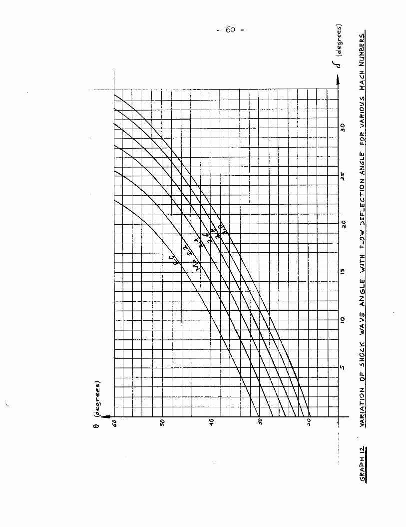
The variation of shock wave angle with flow

deflection angle for various upstream Mach Numbers is

given in chart No. 2 of Ref. 9, Graph 12.

Because an oblique shock wave acts as a

normal shock to the component of flow perpendicular to it,

the f ollowi ng relations f or nor ma l shocks apply t o

oblique shocks if M1 and M2 are replaced by their normal

components M1sin9 and M2sin(9-5 ).

- 11 -

The relations are:

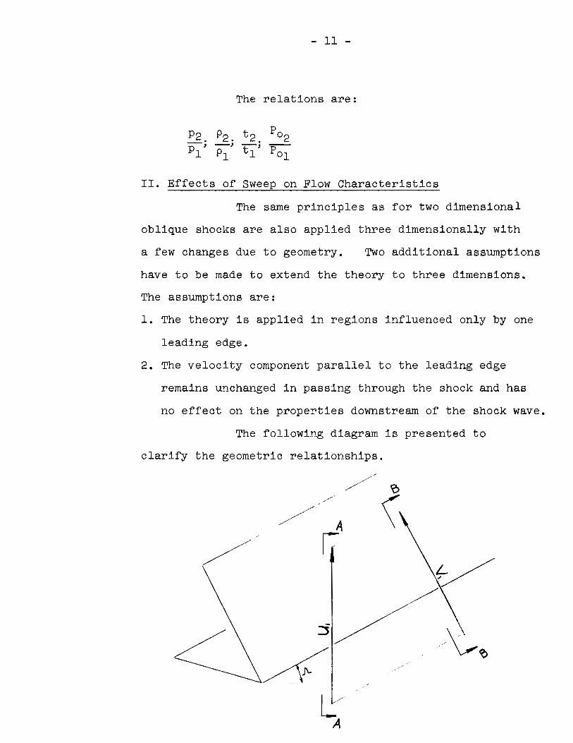
II. Effects of Sweep on Flow Characteristics

The same principles as for two dimensional

oblique shocks are also applied three dimensionally with

a few changes due to geometry. Two additional assumptions

have to be made to extend the theory to three dimensions.

The assumptions are:

1. The theory is applied in regions influenced only by one

leading edge.

2. The velocity component parallel to the leading edge

remains unchanged in passlng through the shock and has

no effect on the properties downstream of the shock wave.

The following diagram is presented to

clarify the geometrie relationships.

A r;-

- 12 -

SECTION A-A .SEC.TIO~ B-S

where ul = Free stream velocity.

a = Streamwise angle of attack.

vl = Total velocity component in plane normal

to leading edge.

A = Sweep angle.

5 = Deflection angle. Angle of attack in plane

normal to leading edge.

As seen from the diagram only two equations

are needed to project the streamwise velocity into a

plane normal to the leading edge and to define the

relation of the three angles a, ...IL and 5.

The equations are:

tana = tan5. cosJL

After transforming Ul; a and JL into V 1 and 5

the process applied is identical to that for two dimensional

oblique shocks.

- 13 -

The total velocity downstream of the

shock wave (u2 ) is composed of the velocity in plane

normal to the leading edge and the velocity parallel

to the leading edge.

View in plane of free stream velocity and leading edge.

From the geometry

2 2 == v2 + w

View in plane of flat ,. surface.

Thus the air stream characteristics outside

of the boundary layer are defined.

C) Heat Transfer Between Air Stream and Surface

Incompressible formulae are valid for

compressible flow at the wall. The theoretical

dimensionless heat transfer coefficient between air

stream and surface may be calculated as follows.

For compressi ble flow the mean friction

coefficient is

- 14 -

This, according to the relation between skin friction

coefficient based on wall temperature and on free

stream temperature, can be written

having taken the exponent in the viscosity temperature

relationship to be equal to 0.8.

From this

( too) 0.1

Croo ~ == 1.328 tw

The heat transfer coefficient

KH~= Nu - 1 cr~~ .........

Pr2/3 Pr vRe" 2

Substituting for Cfoo~oo

For Pr = 0.72 this gives

The amount of heat transferred to the surface by

convection is then given by

This result indicates that t the equilibrium wall w

temperature must be known before the heat transferred

to the surface by convection can be obtained theoretically.

- 15 -

The equilibrium temperature can be calculated assuming

there are no internal heat conduction effects. Then,

for equilibrium, heat gained by convection equals heat

lost by radiation. _1

3600 Cpw p2u2 0.827 Re2

The solution of this equation gives the theoretical

equilibrium wall temperature.

D) Effect of Sweep Angle on Aerodynamic Heating

To determine the effect of sweep angle

on aerodynamic heating, the following theoretical

example was worked out:

Steady free stream conditions were assumed.

Varying only the sweep angle the flow characteristics

outside the boundary layer were calculated.

Graphical solution of equation (a) gave both the

equil1br1um surface t emperature and the heat transferred

to the surface.

The numerical example was:

Wedge airfoil- made of stainless steel. Wedge angle 22°.

Surface size 2 ins. x 1 1/4 in.

Length of sharp leading edge 2 ins.

Free stream conditions - Mœ = 2 .6

Stagnation pressure P0

= 80 psia

Stagnation temperature T0 = 600°C = 1572°R.

- 16 -

Angle of attack in plane normal to leading edge

constant at 5°.

The sweep angle was varied from 0° to 35° in five

degree increments.

The flow characteristics outside the boundary layer were

calculated from isentropic and oblique shock relations

and are presented in the following table: (page 17)

Solving equation (a) graphically, the

equilibrium wall temperature tw and the heat transferred

to the surface Qc were found to be the following

_A_ tw Qc ( 0) (OR) (BTU/ft2 hr)

0 1413.8 3453

5 1413.8 3453

10 1413.4 3449

15 1413.0 3440

20 1411.8 3432

25 1410.9 3425

30 1410.4 3420

35 1408.3 3400

Sample calculations are presented in Appendix I and

Appendix 2.

The results indicate that although equili-

brium wall temperature and heat transferred to the

surface decrease with sweep angle, the effect is

Jl M2 u2 t2 p2 P2U2 Taw 112 Re ( 0 ) (-) (ft/sec) (OR) (lb/ft3) 'lb (OR) l b (-)

ft2sec (ft.sec)

0 2.38 3169.7 737.245 2. 0616xl0-2 65. 3094 1447.173 1 .. 5636xlo5 2.175xl05

5 2.3819 3170 737.111 -2

2.0502xl0 64.9931 1448.06 1.5632x105 2.178xl05

10 2.3834 3171 736.68 2.0453xl0-2 64.8582 1448.09 1. 5630x1o5 2. 20xlo5 1

-2 1--'

15 2.3869 3173.4 735.64 2.038x10 64.6861 1448 .136 1. 5609xlo-5 2. 23xlo5 -..;}

20 2. 3965 3177.8 732.041 2. 0259xl0-2 64. 3799 1446.784 1. 5559xlo-5 2. 29xlo5.

25 2.398 3180 731.663 2. Ol68xlo-2 64 .1358 1446.913 1. 5549xlo-5 2. 43xlo5

30 2.4034 3183.8 730.306 2.0Cl3xlo-2 63.7194 1447.445 1. 553lxlo-5 2. 50xl05

2.4125 3188.67 -2 1446. 528 1. 548lxlo-5 2. 65xlo5 35 727.120 1.9860xl0 63.3278

- 18 -

negligible even at large sweep angles. In fact, the

effect of sweep angle .. is so small that it lies within

the accuracy limits of the experiment.

can be shawn theoretically only.

Thus the effect

In the above example the calculation of

flow characteristics was carried out on a desk calculator

to eight figures ,- acc.uracy.

- 19 -

EXPERIMENTAL APPARATUS

A) The Main Test Facility

The experiment was carried out on the test

facility of the Hypersonic Research Laboratory of McGill

University. The test facility consists of a zirconia

bed heat exchanger operating at temperatures up to 2200°C

and pressures up to 100 psia. The pebble bed is heated

with propane burning in preheated air. The vacuum system

which consists of two stages of steam ejectors followed

by a mechanical pumping stage can provide a test section

pressure of 0.5 psia. at full mass flow.

air mass flow is 0.1 lb/sec.

B) Nozzle and Wedge

The maximum

A Mach Number 2.58 stainless steel nozzle

mounted on the exit of the pebble bed heat exchanger

produced a uniform parallel flow.

nozz1e was 1 in. x 1/2 in.

The exit area of the

The 2 in. wide, 1 1/4 in. high surface

size wedge was made of one 1/16 in. and one 1/32 in.

thick stainless steel plate ( See pD,~t~ no~) J-) • The two

plates were welded together along the leading edge

forming a wedge angle of 22°. Forty, equally spaced

holes, (1/4 in. apart) were drilled into the 1/16 in.

thick side. 28 gauge fiberglass insulated chromel-

alumel thermocouples were lead through the holes from

- 20 -

inside of .the wedge and were welded to the outside

surface. After the welds had been completed the surfaces

were ground and polished to a smooth finish. The final

thickness of the side holding the thermocouples was 3/64 in.

The leading edge was sharpened to a radius of 0.0006 in.

(See wedge on photo No. 1). The thinner surface of the

wedge served simply to protect the thermocouples.

The inside surface of the instrumented

plate was covered with heat resistant cement, providing

both insulated plate and solid support for the thermocouples.

Finally the wedge was placed just outside the exit plane

of the nozzle so, that both the angle of attack and

sweep angle were adjustable (See photo No. 2).

C) Instrumentation

The instrumentation of the main test

facility is given in Ref. 11.

A Honeywell Brown Heiland Direct Recording

Visicorder recorded the following readings of the present

experiment.

Stagnation Pressure.

Stagnation Temperature.

Manifold Pressure. (Test section pressure)

Wedge Surface Temperatures.

Visicorder data: Recording speed 1 in./sec.

14 channels

Sensitivity 0.414 mv/in. with Mll0-350

galvanometers.

- 21 -

6 in. Full scale

Overall system accuracy 1%.

Two channels recorded the readings of the

40 wedge surface thermocouples through two uniselector

switches. In this way all 40 readings were recorded

every 4 seconds.

The air stagnation temperature was measured

upstream of the nozzle by an 18 ga chromel-alumel thermo­

couple.

The stagnation pressure upstream of the

nozzle and the test section pressure were measured by

means of Statham strain gauge pressure transducers

connected to the Visicorder through bridge circuits.

- 22 -

TEST PROCEDURE

A) Operation Technique

The operation process of the main test

facility is summarised in the following steps.

1. Heating of the pebble bed by air from a heat

exchanger, until equilibrium is obtained at the

maximum heat exchanger rating.

2. Ignition of the propane burner. The propane-air

ratio controls the heat in the bed.

3. Closing of propane, heat exchanger and exhaust

valves.

4. Turning on the vacuum pumps and steam ejector in

order to obtain maximum vacuum in test section.

5. Increase of the air supply pressure by the flow control

valve. The air flow is controlled manually to obtain

the required nozzle pressure as indicated by a gauge.

B) Calibrat~on of the Nozzle

Actual dimensions of the supersonic stainless

steel nozzle were

Exit area

Throat area

0.991 in. x 0.508 in ..

0.991 in. x 0.166 in.

These give an area ratio of 3.06.

According to the isentropic relation the

Mach Number of the nozzle should be 2.66.

- 23 -

The actual operating Mach Number of the

nozzle was found by calibration. By the use of pitot

pressure and total pressure tubes the upstream static

and downstream total pressures were measured at 9 points

of the exit plane of the nozzle. Mach N1oobers then were

ca1culated by Rayleigh's supersonic pitot formula

P2 = ( 'Y+l M 2)\~~( 2'Y M 2 _ 'Y-1)'Y~ 1 pl 2 1 ~ \ 'Y+1 1 'Y+1

The average of the obtained Mach Numbers

was taken as the operating Mach Number of the nozz1e.

The results were

( 1.,5 .. r .,s··t

+ t

+ + f + '

8 +

7 +

9 +

S~ALë 2. 11 .. 1"

Points

l

2

3

4

5

6

7

8

9

37.4

37.1

37.7

35.9

35.3

35.7

37.7

37.4

37.7

P_l

4.22 8.86

4.10 9.05

4.20 8.98

3.90 9.20

3.75 9.40

3.90 9.15

4.25 8.86

4.15 9.0

4.20 8.98

Average Mach Number 2.58.

C) Measurements

2.55

2. 58

2.57

2.60

2.63

2.60

2.55

2.58

2.57

The aim of the experiment was to find the

temperature distribution on a wedge having flat surfaces

in the presence of angle of attack and sweep angle.

- 24 -

Efforts were made to maintain constant stagnation

pressure, stagnation temperature and test section pressure

during the whole experiment. The experiment consisted

of eight separate tests. The sweep angle varied from

0 to 35 degrees with 5 degrees increment for each test.

First a simpler wedge than the one described

in section titled Nozzle and Wedge was designed for the

experiment. The shortcomings of the first model made

necessary a new design. The first wedge was made of

mild steel. Although the stagnation temperature of the

air never exceeded 800 degrees centigrade, surface

oxidation and damages on the leading edge were apparent

already after the first few tests. Furthermore there

were only five thermocouples measuring the surface

temperature. The thermocouples were located in the

approximate direction. of the air flow. The results

indicated that the readings of only five thermocouples

give very little information about the actual surface

temperature distribution. So the conclusions drawn

from the first test led to the design of an other wedge.

The second wedge was made of stainless steel with forty

thermocouples reading the surface temperature distribution.

This second wedge performed very well

during the whole experiment. The leading edge remained

sharp ànd;str~i~ht ~ The surfaces needed re-polishing

from time to time, this was done by fine sand paper, to

ensure that the radiation emissivity factor of the surface

- 25 -

would remain constant. Steady state conditions were

reached approximately two minutes after starting a test.

- 26 -

RESULTS

A) Flow Characteristics

The characteristics of the supersonic

free stream were the following.

Mach Number 2.58.

Sweep angle Stagnation Manifold Stagnation pressure pressure temperature

...À.(o) P (psia) p (psia) To (oc) 0 rn

0 80.67 9.05 768

5 82.4 9.75 606

10 81.85 7-5 768

15 81.85 9.4 683

20 82.6 9.48 675

25 82.6 10.0 784

30 81.2 9.44 635

35 81.0 9.15 800

5 the angle of attack in a plane normal to the leading

edge was kept constant at 5 degrees in all cases.

From the above data, using the relations

of isentropic flow and of oblique shock waves, the

required flow characteristics downstream of oblique

shocks were calculated.

A detailed sample calculation is presented

in Appendix 1.

- 27 -

The flow characteristics outside the

boundary layer were:

..A. M2 u2 t2 P2 Taw

( 0) (-) (ft/sec) (OR) (lb/ft3) (OR)

0 2.359 3445 884.2 1.770X.l0""2 1708

5 2.36 3170 750 2.145xlo-2 1462

10 2.361 3450 887 1.805xlo-2 1730

15 2.37 3305 811 1 .. 955xlo-2 1586

20 2.376 3298 802 1.973x10-2 1572

25 2.38 3475 893 1. 76:0.xlo ':2 1752

30 2.385 3240 765 -2 2 .OOOxlO"- 1502

35 g/L!-2 3535 890 1.668xlo-2 1775

As it can be seen the stagnation tempera-

ture of the air varied considerably during the experiment.

The stagnation and manifold pressures could be kept

near constant values.

B) Theoretical Equilibrium Wall Temperature and Heat Transfer to the Wedge

It was developed in the Theoretical Discussion

of the present report that the theoretical equilibrium

surface temperature may be calculated solving the

equation:

where the left hand side of the euqation represents the

heat transferred to the surface by convection, the

- 28 -

right hand side is the heat radiated away from the

surface.

For solving this equation, in addition to

the previously calculated flow characteristics, the

Reynolds Number has to be calculated for each case.

The values of the Reynolds Numbers are:

..A. Re ( 0) (-)

0 1.796xlo-5

5 2.220xlo-5

10 l.84oxlo-5

15 2.090xlo-5

20 2.185xlo-5

25 1.970xlo-5

30 2.43lxlo-5

35 2.155xlo-5

Sample calculation is given in Appendix 2.

The mixed order equation expressing the

theoretical heat balance was then solved graphically for

each case. The intersection points of the convective

heat curves with the radiation curve give both the

theoretical equilibrium wall temperatures and the heat

transferred to the wedge surface by convection (Graph 11).

- 29 -

The final theoretical results are:

...IL tw Qc ( 0) (OR) (BTU/ft2hr)

0 1652 6375

5 1427 3600

10 1672 6690

15 1540 4830

20 1527 4680

25 1687 6970

30 1461 3940

35 1704 7250

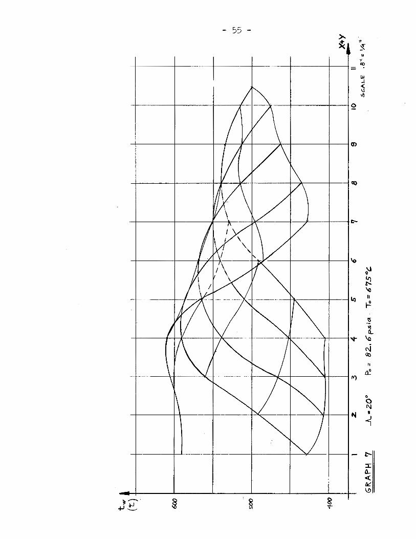
C) Measured Surface Temperature Distribution

The steady state surface temperature

distribution~obtained in the experiment are shown in

graphs 3 to lO .. The method of carpet plotting was

applied in order to obtain a perspective view of tempe-

rature distribution over the whole surface.

Diagram ·l shows the arrangement of wedge

and nozzle in the case of zero sweep angle.

The X and Y axes were taken as indicated.

On the graphs the X+ Y values are indicated along the

abscissa, the measured surface temperatures along the

ordinate. The X = constant and Y = constant points

are connected by continuous curves.

- 30 -

AIR sri?EAH

+ -t +

+ + + -t + t " ~ -t + + -+ + + x

..... ~

DIAGRAM

D) Correction for Heat Conduction Effects

As indicated on the diagram above, only

a relatively small part of the wedge was in the air stream.

The large and irregular variation of heat conduction

effects, made it impossible to evaluate results for

each 1/4 in. square surface separately. After a thorough

investigation of these effects it has been found that

an overall average surface temperature must be taken

as equilibrium wal l temperature. This means average

surface temperature within the air stream.

The surface element so representing the

wedge is the 1/4 in. wide strip in the centre of the

stream, the length of which varied with sweep angle .

This central strip is bounded on the two sides by also

- 31 -

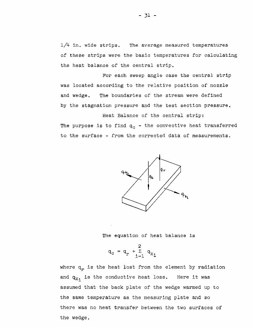
1/4 in. wide strips. The average measured temperatures

of these strips were the basic temperatures for calculating

the heat balance of the central strip.

For each sweep angle case the central strip

was located according to the relative position of nozzle

and wedge. The boundaries of the stream were defined

by the stagnation pressure and the test section pressure.

Heat Balance of the central strip:

The purpose is to find qc - the convective heat transferred

to the surface - from the corrected data of measurements.

The equation of heat balance is

2 qc = q + ~ q

r i=l ki

where qr is the heat lost from the element by radiation

and qki is the conductive heat loss. Here it was

assumed that the back plate of the wedge warmed up to

the same temperature as the measuring plate and so

there was no heat transfer between the two surfaces of

the wedge.

- 32 -

The material constants are:

coefficient of heat conductivity k = 19 (BTU/hr.ft°F)

radiation emissivity e = 0.5.

With these values

where A = ( 1/4 y( length of strip )x( l/144) ( ft2 ).

where Al = A2 = (3/64)x(length of strip)x(l/144) ( ft 2 ).

t = average temperature of centre strip. w

tsi= average temperature of side stri p.

x = distance between centerlines of strips=l/4 in.

E~ Measured Hea t Transfer t o t he Wedge

The average values of the measured strip

temperatures are ..A_ tS _l tw ts2

( 0 ) ( OR) (OR) ( OR)

0 1533 1500 1509

5 1382 1414 1404

10 1594 1613 1577

15 1480 1496 1474

20 1493 1517 1496

25 1525 1530 1522

30 1372 1385 1364

35 1540 1564 1554

- 33 -

With these values the components of the

heat balance equation of the central strip are

0

5

10

15

20

25

30

35

qr

(BTU/hr)

10.81

7.55

12.88

9.71

10.6

11.45

8.01

13.73

qkl

(BTU/hr)

0.5165

0.976

0.587

0.5

0.726

0.199

0.166

0.93

qk2

(BTU/hr)

1.242

0.3054

1.113

0.687

0.6792

0.24

0.744

0.3

qc = =qr+qkl+qk2

(BTU/hr)

11.535

8.831 -

14.58

10.897

12.00

11.959

8.92

14.96

Qce the convective heat in BTU/ft2hr units

is equal to qc.(l/A). The corrected equilibrium wall

temperatures corresponding to Qce were read from graph 11.

Comparing the theoretical and the corrected

experimental results: (twt-twe)lOO A twt twe ( 0) (trieoretical) (experimental) (~Jt (OR) (OR) 0 1652 1578 4.89

5 1427 1470 3.02

10 1672 1667 0.298

15 1540 1542 0.13

20 1527 1568 2.68

25 1687 1548 8.23

30 1461 1420 2.8

35 1704 1595 6.28

- 34 -

À Qct Qce (Qct- Qce)lOO ( 0 ) (theoret~cal) (experimental)

~~~ (BTU/ft hr) (BTU/ft2hr)

0 6375 5320 16.5

5 3600 4050 12.5

10 6690 6610 1.195

15 4830 4840 0.207

20 4680 5190 10.9

25 6920 4960 28.5

30 3940 3520 10.65

35 7250 5560 20.6

- 35 -

DISCUSSION

A) Evaluation of Theoretical and Experimental Results

Before evaluating theoretical and experi­

mental results, the methods by which these results

were obtained have to be evaluated.

Heat transferred to the wall is controlled

by complex phenomena in the boundary layer. Up to the

present time there is no unique method for theoretical

calculation of heat transfer in compressible flow.

Many attempts have been made in the last

fifty years- since Blasius started the analytical

investigation of laminar boundary layer - to solve the

fundamental partial differentiai equations of compressible

flow, the continuity, momentum, and energy equations.

The differences between the assumptions used in the

analyses and between the various mathematical transforma­

tions of variables - in order to reduce the differentiai

equations - result in different solutions. Factors

which can only be obtained experimentally, like Prandtl

Number and Recovery Factor, have always to be included

in the theoretical investigations. Blasius' reliable

formulae for incompressible flow are still the bases

to which modifications are applied to obtain formulae

applicable for compressible flow. The sa obtained

theoretical results are then tested by experiments which

often prove that further modifications are needed.

- 36 -

The theoretical method in the present work

was adopted mostly from Ref. 3 which in itself is a

conclusion of various works, as it was discussed in this

report under the title Review on Boundary Layer Research

Concerning Heat Transfer.

The method of determining heat :transfer

to the surface of the wedge experimentally was based on

the consideration that in steady state the heat transferred

to the surface by convection had to be equal to the heat

radiated away from the surface plus the heat conducted

away within the plate. Therefore the steady state

readings of the surface thermocouples and the. material

constants provided all the necessary information.

The original plan was to evaluate the

heat transferred to every 1/4 square inch of the surface

separately. In this way more refined observations

could have been made concerning the aerodynamic heating

as a function of also the distance from the leading edge.

It was not possible to evaluate results in this way

because the small supersonic air jet, provided by the

nozzle, covered little more than one quarter of the

wedge surface. Temperature gradients due to heat

conduction were present even in the section of the

surface covered by the flow. At sorne places the

effect of conductive heat flow was so large - due to

the comparable sizes of the surface and cross sectional

areas- that the~heat balance equation gave negative

conductive heat.

- 37 -

These effects were eliminated by taking

the average temperature of the surface covered by the

flow as reference temperature rather than the readings

of individual thermocouples. Even so the main purpose

of the experiment - to determine convective heat transfer

experimentally and to compare i t to· theoretically obtained

results - could be carried out fully.

Thus the 1/4 in. wide strip running along

the centerline of the part of the wedge covered by the

flow represented the wedge surface. Evaluation of the

heat balance of this strip under steady conditions in­

dicated that the conductive terms were of the order of

lü% of the radiation term. This approaches the assumption

made in the theoretical investigation where the conductive

heat flow was assumed to be negligible compared to the

radiation term.

Comparing the theoretical and the experi­

mental results we find very good agreement between

equilibrium wall temperatures. Although, as was

mentioned before, the theoretical method itself contains

empirical factors it is considered to hold and to be

applicable as the foundation of the investigations.

The per cent deviation between the theoretical and the

experimental equilibrium wall temperatures lay within

the accuracy limits of the experiment. The accuracy

limits can be approximated to be in the order of 10

per cent.

- 38 -

The exponential radiation curve explains

the increase of per cent deviation when the aerodynamic

heating is expressed in terms of convective heat

transferred to the surface.

A minor but interesting point would have

been to see how well experiment follows the conclusion

of the strictly theoretical investigation that sweep

angle has only negligible effect on aerodynamic heating.

For this the free stream characteristics should have

been the same for every sweep angle. In the present

experiment there were no means to fulfill these

requirements.

A remark is needed concerning the curves

of experimental temperature distribution on the wedge

surface. As the curves indicate, fairly regular tempera­

ture distributions were observed over the plate except

for the readings of the thermocouple row closest to the

leading edge. To explain the meaning and significance

of these unregularities a detailed investigation of

stagnation point heating would be necessary. An

investigation like this could be the subject of a separate

thesis work.

B) Sources of Errors and Instability

Errors arose from two major sources and

their combined effect may have caused errors in the

results. The two main sources were the shortcomings

of the experimental facilities, and the possible

- 39 -

inaccuracies in the approximated factors in the

calculations.

The first type, the experimental errors

are the more significant ones. No steady free stream

conditions could be maintained during the experimenta.

The main facility had no stagnation temperature control

and the stagnation pressure was controlled manually.

The vacuum system was not able to provide constant

vacuum in the test section. To assure that the air

jet would remain supersonic even after sorne pressure

had built up in the test section maximum possible

stagnation pressure was needed. The visicorder readings

indicated that steady state conditions were reached

after about one and a half to two minutes of "running" .

and by that time gradual decrease in stagnation pressure

and temperature could often be observed. These variations

were in the order of two to three per cent. To this

there may be added the measuring accuracy of the

visicorder, the effect of possible error in the calibration

of the visicorder, possible error in reading the baro­

metric pressure, and also the error in reading the

visicorder curves.

Larger errors than the above ones were

included in the readings of the wedge surface thermo­

couples . To test the thermocouples they were placed

into an oven and kept there on constant 600°C tempera-

ture. Their readings on a voltmeter indicated a

- 40 -

maximum +6% deflection from the average reading. This

test was made before the thermocouples were welded to

the surface. The same test was repeated also after the

thermocouples were welded into place and the surface of

the wedge was polished. In this second case an increase

in the deflection of the thermocouple readings was

observed, this time the maximum deflection was +8%. In

the actual experiment added errors may have resulted

from the imperfection of the wire connections between the

wedge surface thermocouples and the visicorder. Here

again the effect of visicorder inaccuracy may have

contributed to the errors. The tnstability of jet

boundaries due to the gradual increase of pressure in

the test section also effected the readings of the

surface thermocouples.

Errors may have been made in the calculations

by assuming that the radiation emissivity factor of the

wedge surface did not change during the experiment.

Efforts were made to keep the wedge surface in uniform

condition, but because the emissivity factor varies

sensitively wi th surface conditions its va lue may have

changed during t he time i nterval of a tes t .

Possible sources of small errors in

calcula tions ar e the empiri ca l factors e. g . Prandtl

Number and fl ow viscosi ty. The se errors may be as sumed

to be the smallest in order of magnitude compared to

the others, be cause the extensive experimental wor k of

- 41 -

noted researchers provide good approximations for these

factors as functions of temperature.

The shock angle of the oblique shock

attached to the leading edge of the wedge was read from

a chart. This may include other small errors, but

because mathematical computation of shock angles is

extremely laborious, large scale charts are generally

used to define them.

Summing up the effects of errors and

~nstabilities the overall accuracy of the experiment

can be estimated to be in the order of +lü%.

- 42 -

CONCLUSIONS

Concluding this work it may be stated

that a theoretical and experimental investigation of

aerodynamic heating of a swept back airfoil was carried

out successfully.

The deviations between theoretical and

experimental results did not exceed the accuracy limits

of the experiment. It has been found that, in the case

of constant 5 degrees angle of attack in a plane normal

to leading edge, the effect of sweep angle on aerodynamic

heating could be considered negligible.

It is suggested that further work concerning

aerodynamic heating of wedge airfoils could be extended

into two separate directions.

One direction should be the investigation

of stagnation point heating, including the vicinity

of the leading edge. This would be necessary because

supersonic heat transfer relations do not hold for

regions of small Reynolds Numbers.

The second direction could be the extension

of the present work, to investigate the effect of

varying angle of attack in plane normal to leading edge.

In this way more general conclusions could be made

concerning the effect of sweep angle on aerodynamic

heating.

- 43 -

APPENDIX I

Sample Calculation of Flow Characteristics Downstream of Shock Wave

Data of experiment:

Sweep angle = 5° = Jl

Angle of attack in plane normal to leading edge = 5o = 5.

Stagnation temperature T0 = 606°C = 1583 °R

Stagnation pressure P0=P1 = 82.4 psia.

Free stream Mach Number Moo = 2.58

According to isentropic relations for M~ = 2.58

Static temperature t 1 = 0.42894

Static pressure p1 = 0.05169

Velocity of sound in free stream

T0 = 679°R

P0

= 4.26 psia.

8.oo =yi''Y.R.g.t1 =v'l.4x53.3x32.2x679 = 1278 ft/sec

Free stream velocity

U00 = aoo. M00 = l278x2. 58 = 3295 ft/sec

The relation of streamwise angle of attack a, with

angle of attack in plane normal to leading edge 5,

and with sweep angle JL is

tana = tan5 • cosJl

from this

Projection of free stream velocity into plane normal to

leading edge

V 1 = U00 /1- co sa sin2 _A_ =3295 J1- 0. 99245x0. 007604 =

= 3280 ft/sec.

- 44 -

Mach Number in plane normal to leading edge

M1 = v1 = ~ = 2.566 aoo ..LC. 1 u

For M1=2.566 and 5 = 5° the shock angle from chart No. 2

of Ref. 9: ..

Velocity component normal to shock wave, upstream of

shock

u1 = V1sin9 = 3280 x 0.4524 c 1484 ft/sec.

Velocity component parallel to shock wave

v = V 1 cos9 = 3280 x 0. 8918 = 2925 ft/sec

Velocity component normal to shock wave, downstream of

shock

u2 = u tan(9-5) = 1484 o.4020 = 1177 ft/sec 1 tan9 0.5073

Velocity in plane normal to leading edge, downstream of

shock

Total velocity downstream of shock

u.2

= ~:} + w2 = /9,_.9-6-.-2-x-l o__,4_ +_l_0_85_x_l_o-:-4---1-0-7 5_x_l_o--,-4 = 3170

ft./sec.

where W - V { = veloci ty component parallel to

leading edge .

I n or de r to u se the simple nor mal shock r elations for

finding flow characteristics downstream of shock, the

Mach Number normal to shock wave has to be defined

Mn= M1sin9 = 2 . 566x0.4524 = 1.162

- 45 -

Now according to normal shock relation for Mn = 1.162

static temperature downstream of shock

Velocity of sound downstream of shock

Mach Number downstream of shock

M2 = u2 = 3170 - 2 36 a2 1343 - •

For the heat transfer calculation, the density of flow

downstream of the shock is also needed.

P = 1.2756 p = 0.02145 lb 2 1 ~

where p1 P1 = 4.26xl44

R t 1 =5=-3 --=. 3=-x_,.6...,..7"""'"9 = 0.0167 lb ft3

Mass velocity

= 67 lb ft2sec

The adiabatic wall temperature

For ~ = 1.162

( 'Y-1 2) ( 8) 46 0 Taw = t 2 l+r~ M2 = 750 1+0.17x5.5 = 1 2 R

where r = recovery factor = y'Pr = ,;o:r2 = 0. 85

The development of this last relation is given in Ref. 10.

- 46 -

APPENDIX II

Sample Calculation of Theoretical Equilibrium Wall Temperature and Heat Transfer

The heat balance equation of the surface

in supersonic air flow

has to be solved.

Where e the radiation emissivity factor of the surface

is 0.5

~ the Stephan Boltzman coefficient is O.l73xlo-8 BTU ·

(ft2hr 0 R4)

The previously calculated flow characteristics

in the case of 5 degrees sweep angle were

t2 = 750 OR

Taw = 1462 OR

u2 = 3170 ft/sec

p2 = 2.145xlo-2 lb/ft3

P2·u2 = 67.0 lb/ft2sec

Re = u2 _.x

1-L

P2

where x, the characteristic length is the distance

from leading edge to the centre of .:f1ow '.' Cove.red

length measured in the direction of main stream

veloci ty (u2 ).

- 47 -

The velocity components of the flow outside

the boundary layer are

where W = velocity parallel to

leading edge

v 2 = velocity normal to

leading edge

Therefore the angle of deviation of the main velocity u2 from the direction normal to the leading edge is given by

~=arc cosv2 = arc cos3156 = arc cos 0.995 = 5.7° u 2 3170

And xJ the distance from leading edge to the centre of

flow covered length of the wedge is

x = 1.25 2x0.995 = 0.6155 in.

The viscosity is calculated from the relation

given in Ref. 9 l. 5 1.5 -8

4 t2 1 -8_ 4 750 x 10 ~ = 73 · 09 t2+198.6 ° - 73 · 09 750+198.6 =

And so the Reynolds Number is

u2.x 3170 o. 6155 Re = ~ = 1.575xlo-5

P2 2.145xlo-2 12

= 2.22xlo5

Substi tut i on i nto t he heat balance

equation gives

1.575xlo-5

lb ) (ft.sec

- 48 -

Substituting chosen values for tw, and

the corresponding specifie heats, the left hand side

of the equation gives at

tw (oR) BTU ) Qconvective ( 2· . ft hr

1410 5390

1420 4380

1430 2350

1440 2310

1450 1240

The right hand side of the equation is

the same for all cases. Calculating the curve for the

whole required range gives

tw( oR) Qradiative( B~ ) ft hr

1100 1250

1200 1780

1300 2460

1400 3320

1500 4360

1600 5660

1700 7190

1800 9050

These curves and the ones representing

convective heat transfer, calculated similarly for the

other values of sweep angle , are presented in graph No •. Yl~

- 49 -

The equilibrium wall temperature and

convective heat transfer can be read from the graph

corresponding to the intersections of the curves Qc and

Qr· In the case of 5 degrees sweep angle these readings

are

t = 1~27 °R w .

0,6

o.s

0.1

.0

§'JSAPH

~~

1,2

1,0

0,

O.l

o. 0

G~APM 2.

- 50 -

Kf'T" Vo11 I<'•I'M.;III'I 4. -r_.lel'l

Il• E 8ra1~~ ,..,/ 4- ev..II\Oo~s

c é:_.,-oc.c. o

1-l l,'v/ H..."'t.~sc.he ~ we..,..,~

c f li Copc .f !4c;o~ .. ~ .. ~e

VD Vc;o~>'l D.-icst:

10

Vl ... 8 P~ al (t-t 4 W)

{K 'T) \

\ OI.UO~I.4riON eQ~H.f81tiUM

n • f,(T) p,. • fa.(r} 1;.•4oo•t

n= . sos

IZ. ,, 18 20

.St<IN Fltl~TIOIIJ ON AN !N.SULATEb FLAT PLATE \VITH NO 1\ADIAT tON

10 12.. If 16 18 20

t-fEAN .SKIN f~IC::TION C::OfFFIC::IENT FO~ L.At-IINAR BOI..lND"-IIt.Y L.A"tE ~

01= A '-Ot-1PitE.SSIBL!' FLUID f::LO'WIN<:; AL.ONt# A Fl..AT PLATE; P..~.?S

n ... sos

- 51 .:.

----------~------~------~------+-------,_-r----1-~

"'

li)

'or

....

~

..J <

· \) \Il

~ ~ \o ~

h

1-0

~ lA Q..

t-\0 cs ao Il

~

0

0 • ~

::r a. < lk:' \!)

- 52 - li

"' ~

+ -= )( tl)

• _., -...1

~

\.) • \Q c \Q

.,. " ~ Ji Ill

.... ~ v

"' o;)

Il

rtl tf

0 tl) Il

~ <{

- 53 -

-w j "( \) . V)

'o

Ill

'If"

IV)

N

~ ~

~ H

f!

-~ .., CL Ill ~

~

" tf

0 c • ~

- 54 -

------L-------+--------t-------t~~r---jj-------, =~ ~

0

'-}J CV) 'X)

\0 Ill ,,

~

G' YI

V" o... Û\ ~ -QC)

Il

~ ~

0

Il\

~ Il

~

\o

.:1: (L

< ~ I,D

~ c 0 ~u- c 0 -+) 0 Ill ~

- 55 -

Il

CIO

==

\o

lq

l'lit'

IV)

~

Ul ..J < \) Ill

~ ~ 'a Il

t-! IS Ill IL

\a

c-.J Q:)

•• &

0

0 1\l 1

~

- 56 - :>-.. +' )(

= ~ Il .. ~ .

-w -..~

<( \J Ill

'4)

li)

·or.

~

4i

~ ~ ~ 1::--

Il

~

~

Ill ~

"' ci \'0 If

~

0 ln N Il

~

- 57 ~

Il

~ . lù __ J_ ____ -4---.~4------1------i-----~=~

0 0 li)

0 Q rtl

~

\D

Il)

,..

tf1

f\j

~ LI) dl ... •

Jo!

G ~ Q..

Cil . co

" ~

0 c tf) Il

~

- 58 -

~----~--~~----~----~----~----T--1=

-4------~----~+-----~------~------+-----~r-~9

~

~

T

~

~

-~

~ ~ c ~

H

~

G ~ L

0

~

" ~

0 ~ ~

• ~

0

x ~

< ~

--~----~----~------L-----~----~------~-T--~

- 59 -

Q

(t~~~) t--------t--1-t--~1.----+--' - t--

Il 1 ! \

1

! 1

1 L_~ M00~------4---------+---~~~~-~~~~.~~~~~--~~~~--~--Q <o"v0~v~:=--, - G'

?OOOr-----+i ----1-1~'---~+-j-+--l\ __ : --+--1----*/-H------+--

! 1 i 1 1 1 j //

il 1 l' 1 ! 6000~------~-+~----++~-----+-+--~+-~~-----4--

1.1 1 !

1 '

1 sooo ··------;-! -4---...._---+, --+---+-:./!----, -----+--+-++---+--------11--

i 1

4!000t------...__ 1 +---t-Tj:__i --+-~---4-: - ·----'t--t+l--t--t-r.tt ____ -t---i / : ? ~ i ~ 1 IJ

1 i ~ tv J/ ! i ~ ~ 1~ 1

V o,.

JOOO ----·-· --o;--+--+--,----t---~ -7---_;--i ---+---~-'-~'----+--

~ ~ ' : 1 M ~ ! ' Il

1 j

~ i !

: ' : 1° ! i 2000!---------~-41~~------~----~-------~

! ! 1

!

i 1

; 1

1000~~-------' ------~~----------------~·--------~---t-, I.SOO 1'\00 ISOO 140'00 1700 1800 -

tR.) GRAPH Il THEO!tE'TICAL E:QUILIBRIUM \x/ALL TEMPERATURE5 4.

HtAT TR.AN.S FE'!<:. TO THE 'WALL

-Ill \1

" !... Ul

" ~ -

['.

" ~ !'.. l'

""' f".-

' !'...

!"'-

<:)

"

1

! .......

"' " ["-. '\

" " " "\ r\. r\.

"' '\ '\, 1'\ \ \

•"'- f\. 1\

"' r\ ' "\~ 1\ \

"\ \

"'" \ \ ~ 1'\.

'\ 1\ '\ ~~

cP\_ l''

1\ \

~

- 60 -

' '

+ - f-·-- f-·-· ·- ·· ··- · f-- ·--- - ·- --·· -··· -· .. -1

t -

!

1

[\ i\ 1\

\ \ f\ 1\ 1\

' \

Î\ \ ~( ~ J(\, -.

c ~~ 1\ r-...

i~ \ \ \ t~ ~ 1\ 1\

1~ 1\ \ \, \ \ \ 1\ [\ 1\

\ 1\ \ \ \ \ ' \ 1\ f\ 1\ 1\

\ 1\ \ \ \ \ \ 1\ 1\ 1\

\ [\ \ \ \ 1\ \ 1\ 1\'

\ 1\ \ \ \1\ \ t\' \ 1\ \ 1\ \~

\ \ \ ' ' \ 1\ ~ 1\ \ \ \ \ \1\

1\ \ 1\ \ \ \ 1\ \ \1\

0 ~ () 'l"' ('j

- ·-. -

VI QI

" 1.. \'n QI \J -~

-- ·

1---··

\Il ~ tu 4) :z: ::3 .2 :z. \J <{

r \1)

:::s a & <

0 > IYI

Ill 1'4

0 rot

Il\

0

lt}

lu ...1 ~ z "'(

z 0 1-\) UJ ..J IL

"' a ) 0 .J u..

x 1-)

2 a 1-< oc ~

- 61 -

PHOTO NO. 1

WEDGE INSTRUMENTED WITH THERMOCOUPLES FOR HEAT TRANSFER MEASUREMENTS

- 62

PHOTO NO. 2 WEDGE MOUNTED ON MACH 2.58 NOZZLE

- 63 -

REFERENCES

1. L.L. Moore A Solution of the Laminar Boundary Layer Equations for a Compressible Fluid with Variable Properties, Including Dissociation. Journal of the Aeronautical Sciences. Vol. 19, No. 8, 1952.

2. E.R. VanDriest Investigation of Laminar Boundary Layer in Compressible Fluids Using the Crocco Method. N.A.C.A. T.N. 2597, 1952.

A.H. Shapiro The Dynamics Fluid Flow. Ronald Press

and Thermodynamics of Compressible Vol. 2.

Company, New York, 1954.

4. H.S. Johnson and M.V. Rubesin Aerodynamic Heating and Convective Heat Transfer. A.S.M.E. Vol. 71, p. 447, 1949.

5. J. Kaye Survey on Friction Coefficients, Recovery Factors, and Heat Transfer Coefficients for Supersonic Flow. Journal of the Aero. Sei. Vol. 21, No. 2, 1954.

6. Dr. H. Schlichting Boundary Layer Theory Pergamon Press Ltd., London, 1955.

7. Douglas Aircraft Company, Inc., Normal and Oblique Shock Characteristics at Hypersonic Speeds. Engineering Report No. L.B.-25599, 1957.

8. W.E. Moeckel Oblique Shock Relations at Hypersonic Speeds for Air in Chemical Equilibrium. N.A.C.A. T.N. 3895, 1957.

- 64 -

9. Ames Research Staff Equations, Tables and Charts for Compressible Flow. N.A.C.A. Rept. 1135, 1953.

10. D.R. Chapman and M.V. Rubesin Temperature and Velocity Profiles in the Compressible Laminar Boundary Layer with Arbitrary Distribution of Surface Temperature. Journal of the Aeronautical Sciences Vol. 16, No. 9. 1949.

11. J. Swithenbank Hypersonic Propulsion Research Programme Hypersonic Propulsion Research Laboratory Report No. SCS 8 McGill University, Montreal 1959.

12. F.V. Davies and R.J. Monaghan The Determination of Skin Temperatures Attained in High Speed Flight. Royal Aircraft Establishment. Report No. Aero 2454, 1952.