Aerial Multi-hop Sensor Networks - cister.isep.ipp.pt · Aerial Multi-hop Sensor Networks Luis...
178
Aerial Multi-hop Sensor Networks PhD Thesis CISTER-TR-181003 Luis Ramos Pinto
Transcript of Aerial Multi-hop Sensor Networks - cister.isep.ipp.pt · Aerial Multi-hop Sensor Networks Luis...

Aerial Multi-hop Sensor Networks
PhD Thesis
CISTER-TR-181003
Luis Ramos Pinto

PhD Thesis CISTER-TR-181003 Aerial Multi-hop Sensor Networks
© CISTER Research Center www.cister.isep.ipp.pt
1
Aerial Multi-hop Sensor Networks
Luis Ramos Pinto
*CISTER Research Centre
Polytechnic Institute of Porto (ISEP-IPP)
Rua Dr. António Bernardino de Almeida, 431
4200-072 Porto
Portugal
Tel.: +351.22.8340509, Fax: +351.22.8321159
E-mail:
http://www.cister.isep.ipp.pt
Abstract
Unmanned Aerial Vehicles (UAVs) recently enabled a myriad of new applications spanningdomains from personal entertainment and industrial inspection, to criminal surveillanceand forest monitoring. A combination of sensor collection, wireless communicationand path planning between multiple distributed agents is the natural way tosupport applications. Several small UAVs working collaboratively can rapidly provideextended reach, at low cost, and efficiently stream sensor information to operators ona ground station. A significant amount of previous work has addressed each of thesetopics independently, but in this dissertation we propose a holistic approach for joint coordinationof networking and topology (placement of mobile nodes). Our thesis is thatthis approach improves user-interactive control of UAVs for live-streaming applicationsin terms of throughput, delay and reliability.In order to defend these claims, this dissertation begins by experimentally evaluatingand modeling the wireless link between two UAVs, under different conditions. Dueto limited link range, and the need for wide-area operation, the model is extended toencompass a multi-hop topology. We show that the performance of such networks usingCOTS devices is typically poor, and solutions must rely on coordination of networkprotocol and topology, simultaneously.At the network layer, we introduce a novel Time-division Multiple Access (TDMA)scheme called Distributed Variable Slot Protocol that relies on adaptive slot-length. Weprove its convergence as well as its meliorated performance experimentally validated,namely 50% higher packet delivery. In terms of network topology, we show that withoutnode placement control overall performance of the network is severely penalized, dueto natural link asymmetries. We propose a novel protocol, named Dynamic Relay Placement, that is able to do both online link quality model-estimation and in a distributedfashion decide the best location for each network node, increasing throughput by 300%.Finally, we demonstrate the end-to-end system in a multi-vehicle monitoring mission.We show that coordination of multiple UAVs increases the sensor sampling rateup to 7 times in wide areas when compared to a naive approach. This work considersenvironmental constraints such as wind, as well as the intrinsic limitations of the vehiclessuch as maximum acceleration.

FACULDADE DE ENGENHARIA DA UNIVERSIDADE DO PORTO
Aerial Multi-hop Sensor Networks
Luis Ramos Pinto
Programa Doutoral em Engenharia Electrotécnica e de Computadores
Co-advisor: Prof. Doutor Luís Miguel Pinho de Almeida
Co-advisor: Prof. Doutor Anthony Rowe
May, 2018
The thesis was also submitted to Carnegie Mellon University, Pittsburgh, USA, in partial fulfillment of the requirements
for the Doctoral degree in Electrical and Computer Engineering. The work was supported through the CMU|Portugal
dual-degree doctoral program.

c© Luis Ramos Pinto, 2018

Aerial Multi-hop Sensor Networks
Luis Ramos Pinto
Programa Doutoral em Engenharia Electrotécnica e de Computadores
Dissertation submitted in partial fulfilment of the requirements for the
degree of Doctor of Philosophy in Electrical and Computer Engineering at
the Faculty of Engineering, University of Porto
Approved by:
Co-advisor: Prof. Anthony Rowe, PhD
Referee: Prof. Pedro Ferreira do Souto, PhD
Referee: Prof. Mário Jorge Rodrigues de Sousa, PhD
Referee: Prof. Bruno Sinopoli, PhD
Referee: Prof. Patrick Tague, PhD
April 10, 2018


To my family,
Mafalda
and my daughters
À minha família,
à Mafalda
e às minhas filhas
v


Acknowledgements
I would like to thank my advisors, Luis Almeida and Anthony Rowe, for their sup-
port. Their guidance and knowledge allowed me to pursue my degree of Doctorate in
Philosophy revolving along a topic I truly enjoyed. They have supported, encouraged
and motivated me to work hard along these last years and allowed me to meet other
researchers and their work.
I would like to thank the co-authors of my main publications for their ideas and hard
work namely Luís Oliveira, André Moreira, Sidney Carvalho and Hassan Alizadeh. I
would like to thank the defense committee members for their time and input, namely
professors Patrick Tague and Bruno Sinopoli from CMU, and professors Mario Sousa
and Pedro Souto from FEUP. I cannot express enough gratitude towards the CMU Portu-
gal PhD program, namely the staff for their kindness, and the financial support provided
by the Fundação para a Ciência e a Tecnologia (Portuguese Foundation of Science and
Technology) under grant SFRH/BD/51630/2011.
I would like to extend my gratitude to my colleagues and friends that I met both at
CMU and at FEUP; they have provided me such good times and made my time during
the PhD absolutely great. Lastly, I would like to thank my family, specially my beloved
wife that motivated me 100% to start the PhD. Along with my daughters, they inspire
me and make me the happiest person alive.
vii


Abstract
Unmanned Aerial Vehicles (UAVs) recently enabled a myriad of new applications span-
ning domains from personal entertainment and industrial inspection, to criminal surveil-
lance and forest monitoring. A combination of sensor collection, wireless communi-
cation and path planning between multiple distributed agents is the natural way to
support applications. Several small UAVs working collaboratively can rapidly provide
extended reach, at low cost, and efficiently stream sensor information to operators on
a ground station. A significant amount of previous work has addressed each of these
topics independently, but in this dissertation we propose a holistic approach for joint co-
ordination of networking and topology (placement of mobile nodes). Our thesis is that
this approach improves user-interactive control of UAVs for live-streaming applications
in terms of throughput, delay and reliability.
In order to defend these claims, this dissertation begins by experimentally evaluating
and modeling the wireless link between two UAVs, under different conditions. Due
to limited link range, and the need for wide-area operation, the model is extended to
encompass a multi-hop topology. We show that the performance of such networks using
COTS devices is typically poor, and solutions must rely on coordination of network
protocol and topology, simultaneously.
At the network layer, we introduce a novel Time-division Multiple Access (TDMA)
scheme called Distributed Variable Slot Protocol that relies on adaptive slot-length. We
prove its convergence as well as its meliorated performance experimentally validated,
namely 50% higher packet delivery. In terms of network topology, we show that without
node placement control overall performance of the network is severely penalized, due
to natural link asymmetries. We propose a novel protocol, named Dynamic Relay Place-
ix

x ABSTRACT
ment, that is able to do both online link quality model-estimation and in a distributed
fashion decide the best location for each network node, increasing throughput by 300%.
Finally, we demonstrate the end-to-end system in a multi-vehicle monitoring mis-
sion. We show that coordination of multiple UAVs increases the sensor sampling rate
up to 7 times in wide areas when compared to a naive approach. This work considers
environmental constraints such as wind, as well as the intrinsic limitations of the vehi-
cles such as maximum acceleration.
Keywords: 802.11, ad hoc networks, channel models, monitoring, relay placement, relay
networks, time division multiple access, unmanned aerial vehicle, wireless communica-
tion.

Resumo
Avanços recentes em veículos aéreos não tripulados (UAVs) têm vindo a permitir uma
miríade de novas aplicações, espalhando-se por domínios do entretenimento pessoal à
inspeção industrial, da vigilância criminal à monitorização florestal. Uma combinação
de sensores, comunicação sem fios e planeamento de rotas entre múltiplos agentes dis-
tribuídos é a forma natural de realizar tais aplicações. Vários UAVs trabalhando colabo-
rativamente podem rapidamente fornecer maior alcance, a baixo custo, e eficientemente
transmitir ao vivo informação sensorial para operadores numa estação base, no solo.
Uma parte significativa do estado-de-arte relacionado visa cada um destes tópicos in-
dependentemente, por isso nós nesta dissertação propomos uma abordagem holística
para uma coordenação conjunta do protocolo da rede e da topologia (colocação de nós).
A nossa tese é que esta abordagem melhora a interactividade do utilizador no controlo
de UAVs em aplicações de transmissão ao vivo em termos de velocidade, latência e
confiabilidade.
De forma a defender esta tese, esta dissertação começa por experimentalmente avaliar
e modelar o canal sem fio entre dois UAVs, sob diferentes condições. Devido ao limitado
alcance da ligação, e à necessidade de operação a larga escala, o modelo é completado
considerando para isso topologias multi-salto. Mostramos que o desempenho destas
redes usando dispositivos COTS é tipicamente pobre, e que pode ser melhorado com
uma coordenação simultânea da rede e da topologia.
A nível da rede, propomos um novo sistema de melhoria da comunicação baseado
em TDMA (Acesso Múltiplo por Divisão de Tempo). Este novo protocolo chamado
Distributed Variable Slots Protocol funciona com base na adaptação do tamanho das
slots atribuídas a cada transmissor. A sua convergência é provada, assim como validada
experimentalmente no desempenho melhorado do sistema, nomeadamente 50% mais
xi

xii RESUMO
entrega de pacotes. A nível da topologia, mostramos que sem controlo de posiciona-
mento de nós o desempenho da rede é severamente penalizado devido a assimetrias
naturais dos links. Propomos um novo protocolo, chamado Dynamic Relay Placement
que é capaz de estimar a qualidade das ligações em tempo-real assim como de forma
distribuída decidir a melhor localização para cada um dos nós da rede, aumentando as
taxas de transferência em 300%.
Para finalizar, desenhamos uma missão de monitorização multi-veículo. Mostramos
que com uma cordenação adequada de vários veiculos aumenta em 7 vezes a taxa de
sensorização de áreas extensas quando comparada com uma abordagem mais simples.
Este trabalho considera restrições ambientais tais como o vento, assim como as limi-
tações intrínsecas dos veículos tais como aceleração máxima.
Palavras-chave: 802.11, ad hoc, modelo canal, monitorização, redes sem fio, repetidores,
TDMA, UAV.

Table of Contents
Dedication v
Acknowledgements vii
Abstract ix
Resumo xi
Table of Contents xiii
List of Tables xvii
List of Figures xviii
Notation xxi
Technical abbreviations and acronyms . . . . . . . . . . . . . . . . . . . . . . . . xxi
Units . . . . . . . . . . . . . . . . . . . . . . . . . . . . . . . . . . . . . . . . . . . xxii
Math Expressions . . . . . . . . . . . . . . . . . . . . . . . . . . . . . . . . . . . . xxii
Definitions . . . . . . . . . . . . . . . . . . . . . . . . . . . . . . . . . . . . . . . . xxiii
Other . . . . . . . . . . . . . . . . . . . . . . . . . . . . . . . . . . . . . . . . . . . xxiv
1 Introduction 1
1.1 Unmanned Aerial Vehicles . . . . . . . . . . . . . . . . . . . . . . . . . . . . 1
xiii

xiv TABLE OF CONTENTS
1.2 Context . . . . . . . . . . . . . . . . . . . . . . . . . . . . . . . . . . . . . . . 2
1.3 Team of UAVs . . . . . . . . . . . . . . . . . . . . . . . . . . . . . . . . . . . 3
1.4 Applications . . . . . . . . . . . . . . . . . . . . . . . . . . . . . . . . . . . . 4
1.5 System Challenges . . . . . . . . . . . . . . . . . . . . . . . . . . . . . . . . 7
1.6 Vision and thesis . . . . . . . . . . . . . . . . . . . . . . . . . . . . . . . . . 10
1.7 Goals . . . . . . . . . . . . . . . . . . . . . . . . . . . . . . . . . . . . . . . . 11
1.8 Contributions . . . . . . . . . . . . . . . . . . . . . . . . . . . . . . . . . . . 12
1.9 Organization . . . . . . . . . . . . . . . . . . . . . . . . . . . . . . . . . . . . 14
2 Background 15
2.1 UAV . . . . . . . . . . . . . . . . . . . . . . . . . . . . . . . . . . . . . . . . . 15
2.2 UAV Wireless Sensor Networks . . . . . . . . . . . . . . . . . . . . . . . . . 17
2.3 Network Performance . . . . . . . . . . . . . . . . . . . . . . . . . . . . . . 18
2.4 Medium Access . . . . . . . . . . . . . . . . . . . . . . . . . . . . . . . . . . 21
2.5 Relay Placement . . . . . . . . . . . . . . . . . . . . . . . . . . . . . . . . . . 24
2.6 Applications . . . . . . . . . . . . . . . . . . . . . . . . . . . . . . . . . . . . 25
3 Building an Aerial Multi-hop Network 31
3.1 Problem Statement . . . . . . . . . . . . . . . . . . . . . . . . . . . . . . . . 32
3.2 Link Layer – Experiments . . . . . . . . . . . . . . . . . . . . . . . . . . . . 33
3.3 Link Layer – Model . . . . . . . . . . . . . . . . . . . . . . . . . . . . . . . . 38
3.4 Network – Model . . . . . . . . . . . . . . . . . . . . . . . . . . . . . . . . . 40
3.5 Network – Experiments . . . . . . . . . . . . . . . . . . . . . . . . . . . . . 45
3.6 Multi-hop Network Summary . . . . . . . . . . . . . . . . . . . . . . . . . . 49
4 Self-Synchronized Network TDMA 51
4.1 Synchronization Method . . . . . . . . . . . . . . . . . . . . . . . . . . . . . 52
4.2 Experimental Results . . . . . . . . . . . . . . . . . . . . . . . . . . . . . . . 56

TABLE OF CONTENTS xv
4.3 Synchronization Summary . . . . . . . . . . . . . . . . . . . . . . . . . . . . 58
5 Dynamic Slot-length for TDMA 59
5.1 Problem Statement . . . . . . . . . . . . . . . . . . . . . . . . . . . . . . . . 60
5.2 A Variable Slot-length TDMA Solution . . . . . . . . . . . . . . . . . . . . 62
5.3 Protocol . . . . . . . . . . . . . . . . . . . . . . . . . . . . . . . . . . . . . . . 66
5.4 Convergence . . . . . . . . . . . . . . . . . . . . . . . . . . . . . . . . . . . . 66
5.5 Worst Case Delay . . . . . . . . . . . . . . . . . . . . . . . . . . . . . . . . . 72
5.6 Evaluation . . . . . . . . . . . . . . . . . . . . . . . . . . . . . . . . . . . . . 75
5.7 Dynamic Slot-length Summary . . . . . . . . . . . . . . . . . . . . . . . . . 81
6 Relay Placement 83
6.1 Problem Statement . . . . . . . . . . . . . . . . . . . . . . . . . . . . . . . . 84
6.2 Optimal Relay Placement . . . . . . . . . . . . . . . . . . . . . . . . . . . . 86
6.3 Dynamic Relay Placement (DRP) Protocol . . . . . . . . . . . . . . . . . . . 88
6.4 Experimental results . . . . . . . . . . . . . . . . . . . . . . . . . . . . . . . 90
6.5 Relay Placement Summary . . . . . . . . . . . . . . . . . . . . . . . . . . . 94
7 Aerial Monitoring 95
7.1 System description . . . . . . . . . . . . . . . . . . . . . . . . . . . . . . . . 96
7.2 Optimal Trajectories and Frame-rate . . . . . . . . . . . . . . . . . . . . . . 102
7.3 Distributed Formation Control . . . . . . . . . . . . . . . . . . . . . . . . . 107
7.4 Simulation Results . . . . . . . . . . . . . . . . . . . . . . . . . . . . . . . . 108
7.5 Monitoring Summary . . . . . . . . . . . . . . . . . . . . . . . . . . . . . . 113
8 Drones Software Architecture 115
8.1 Navigation Data, Actuator and Flight Control . . . . . . . . . . . . . . . . 115
8.2 GPS and Autonomous Flight . . . . . . . . . . . . . . . . . . . . . . . . . . 117
8.3 Keyboard . . . . . . . . . . . . . . . . . . . . . . . . . . . . . . . . . . . . . . 119

xvi TABLE OF CONTENTS
8.4 Communications . . . . . . . . . . . . . . . . . . . . . . . . . . . . . . . . . 119
9 Conclusion 125
9.1 Thesis Validation . . . . . . . . . . . . . . . . . . . . . . . . . . . . . . . . . 125
9.2 Future Work . . . . . . . . . . . . . . . . . . . . . . . . . . . . . . . . . . . . 127
Bibliography 131
A Channel Assessment Model 137
B Drone-RK API 141
B.1 Navdata . . . . . . . . . . . . . . . . . . . . . . . . . . . . . . . . . . . . . . 141
B.2 GPS . . . . . . . . . . . . . . . . . . . . . . . . . . . . . . . . . . . . . . . . . 142
B.3 Flight Control . . . . . . . . . . . . . . . . . . . . . . . . . . . . . . . . . . . 143
B.4 Autonomous Flight . . . . . . . . . . . . . . . . . . . . . . . . . . . . . . . . 144
B.5 Packet Manager . . . . . . . . . . . . . . . . . . . . . . . . . . . . . . . . . . 145
B.6 PDR . . . . . . . . . . . . . . . . . . . . . . . . . . . . . . . . . . . . . . . . . 146
B.7 TDMA . . . . . . . . . . . . . . . . . . . . . . . . . . . . . . . . . . . . . . . 146
B.8 Video . . . . . . . . . . . . . . . . . . . . . . . . . . . . . . . . . . . . . . . . 147
B.9 Image Processing . . . . . . . . . . . . . . . . . . . . . . . . . . . . . . . . . 148
B.10 Actuator . . . . . . . . . . . . . . . . . . . . . . . . . . . . . . . . . . . . . . 148
B.11 AR Config . . . . . . . . . . . . . . . . . . . . . . . . . . . . . . . . . . . . . 148
B.12 Keyboard . . . . . . . . . . . . . . . . . . . . . . . . . . . . . . . . . . . . . . 149
B.13 Utils . . . . . . . . . . . . . . . . . . . . . . . . . . . . . . . . . . . . . . . . . 149

List of Tables
3.1 Experiment setup for the two AR Drone 2.0 vehicles in the single-link channel
characterization . . . . . . . . . . . . . . . . . . . . . . . . . . . . . . . . . . . . 34
3.2 Parameters of the PDR model for different conditions . . . . . . . . . . . . . . 39
3.3 Experiment set-up for the AR Drone 2.0 vehicles on the multi hop network
characterization. . . . . . . . . . . . . . . . . . . . . . . . . . . . . . . . . . . . . 46
7.1 Summary of UAV motion equations . . . . . . . . . . . . . . . . . . . . . . . . 100
7.2 Simulation Setup for the Video-monitoring application. . . . . . . . . . . . . . 109
xvii

List of Figures
1.1 Parrot AR Drone 2.0 quadrotor is controlled by a smartphone. . . . . . . . . . 2
1.2 DJI Mavic Pro does obstacle avoidance and allows insertion of external cameras. 2
1.3 Eachine E013 is a low-cost micro quadrotor equipped with camera and FPV
headset. . . . . . . . . . . . . . . . . . . . . . . . . . . . . . . . . . . . . . . . . . 3
1.4 Intel Aero research platform comes with a vast set of external sensors. . . . . 3
1.5 A quadrotor swarm and communication links (red dashed-lines). . . . . . . . 4
1.6 LeddarOne is a LIDAR sensor designed for small UAVs. . . . . . . . . . . . . 4
1.7 Drone view of Pedrogão, Portugal . . . . . . . . . . . . . . . . . . . . . . . . . 5
1.8 Drone view of Santa Rosa, California . . . . . . . . . . . . . . . . . . . . . . . 5
1.9 Indian authorities are considering drones for crowd control. . . . . . . . . . . 5
1.10 Examples of large-scale applications for drone swarms . . . . . . . . . . . . . 6
1.11 List of challenges designing aerial multi-hop sensor networks . . . . . . . . . 7
1.12 Vision of aerial multi-hop sensor network . . . . . . . . . . . . . . . . . . . . . 11
2.1 Diagram of a multirotor with four rotors . . . . . . . . . . . . . . . . . . . . . 15
2.2 A UAV wireless sensor network . . . . . . . . . . . . . . . . . . . . . . . . . . 17
2.3 TDMA allows each node to send packets in their own slots. . . . . . . . . . . 22
3.1 AR Drone 2.0 platform, a common COTS quadrotor, used for the experiments. 33
3.2 Typical PDR value over time. It mimics a Bernoulli experiment. . . . . . . . . 35
xviii

List of Figures xix
3.3 PDR versus distance on different conditions. . . . . . . . . . . . . . . . . . . . 36
3.4 Maximum network throughput as function of distance . . . . . . . . . . . . . 46
3.5 Packet traces captured by a monitor node, using Wireshark(Wireshark, 2016) 48
3.6 Throughput at different end-to-end network lengths . . . . . . . . . . . . . . 48
4.1 Round period time is obtained from the epoch time via modulo operation . 53
4.2 Defining a TDMA slot and respective boundaries . . . . . . . . . . . . . . . . 53
4.3 Node with slot ID 3 estimates boundaries of slots ID 1 and ID 2 . . . . . . . . 55
4.4 Illustration of TDMA self-synchronization mechanism taking place . . . . . . 57
4.5 Example of TDMA self-synchronization mechanism taking place . . . . . . . 58
5.1 Multi-hop Line Network model . . . . . . . . . . . . . . . . . . . . . . . . . . . 60
5.2 Inefficiencies using CSMA . . . . . . . . . . . . . . . . . . . . . . . . . . . . . . 62
5.3 Inefficiencies under TDMA when all time slots are of equal length . . . . . . 63
5.4 Concept of DVSP where each slot has different length . . . . . . . . . . . . . 63
5.5 Handshake diagram of Distributed Variable Slot-length Protocol (DVSP). . . 67
5.6 Example of slot length convergence in a network with four slots . . . . . . . 71
5.7 DVSP convergence with 4 hops . . . . . . . . . . . . . . . . . . . . . . . . . . . 73
5.8 DVSP convergence with 6 hops . . . . . . . . . . . . . . . . . . . . . . . . . . . 73
5.9 DVSP convergence with 10 hops . . . . . . . . . . . . . . . . . . . . . . . . . . 74
5.10 DVSP convergence with 12 hops . . . . . . . . . . . . . . . . . . . . . . . . . . 74
5.11 Different topologies used during the experiments . . . . . . . . . . . . . . . . 76
5.12 Histogram of measured end-to-end delay . . . . . . . . . . . . . . . . . . . . . 78
5.13 Histogram of measured end-to-end packet delivery ratio . . . . . . . . . . . . 79
5.14 Histogram of measured end-to-end goodput . . . . . . . . . . . . . . . . . . . 80
5.15 Snapshot of the video stream at the sink . . . . . . . . . . . . . . . . . . . . . . 81
6.1 Multi-hop line network model . . . . . . . . . . . . . . . . . . . . . . . . . . . 84
6.2 TDMA overlay protocol with each node transmitting in its slot . . . . . . . . 85

xx List of Figures
6.3 Example of optimal solution for the relay position problem . . . . . . . . . . 87
6.4 Optimal PDR and relay placement versus network end-to-end distance . . . 88
6.5 DRP initial state. Relay is 10m away from BS. . . . . . . . . . . . . . . . . . . . 90
6.6 DRP state when relay is 23m away from BS. . . . . . . . . . . . . . . . . . . . 90
6.7 DRP state when relay is 43m away from BS. Estimation matches ground truth. 90
6.8 DRP final state. Relay estimated the optimal location at 57.8m from the Source. 90
6.9 Experiment layout of the UAVs and computer base station . . . . . . . . . . . 91
6.10 Experimental packet delivery ratio measurements . . . . . . . . . . . . . . . . 93
6.11 Video stream snapshot with relay positioned at two distinct locations . . . . 93
6.12 End-to-end throughput at different relay positions . . . . . . . . . . . . . . . . 94
7.1 Overview of the video-monitoring application system . . . . . . . . . . . . . 97
7.2 Model of the Area of Interest . . . . . . . . . . . . . . . . . . . . . . . . . . . . 98
7.3 Networking and topology models . . . . . . . . . . . . . . . . . . . . . . . . . 101
7.4 Proposed optimal trajectory for the UAVs (even case) . . . . . . . . . . . . . . 104
7.5 Proposed optimal trajectory for the UAVs (odd case) . . . . . . . . . . . . . . 104
7.6 Maximum frame rate vs number of UAVs (i) . . . . . . . . . . . . . . . . . . . 110
7.7 Maximum frame rate vs number of UAVs (ii) . . . . . . . . . . . . . . . . . . . 111
7.8 Maximum frame rate vs number of UAVs (iii) . . . . . . . . . . . . . . . . . . 112
8.1 Drone-RK software is comprised of several modules . . . . . . . . . . . . . . 116
8.2 Piksi GPS Basestation . . . . . . . . . . . . . . . . . . . . . . . . . . . . . . . . . 118
8.3 Piksi GPS on a drone . . . . . . . . . . . . . . . . . . . . . . . . . . . . . . . . . 118
8.4 Application layer working diagram . . . . . . . . . . . . . . . . . . . . . . . . 120
8.5 Packet Manager (PM) layer working diagram . . . . . . . . . . . . . . . . . . . 121
8.6 TDMA layer working diagram . . . . . . . . . . . . . . . . . . . . . . . . . . . 122
8.7 Packet encapsulation used in Drone-RK . . . . . . . . . . . . . . . . . . . . . . 123

Notation
Technical abbreviations and acronyms
• 3D: three-dimensional
• AL: application layer
• AoI: area of interest
• BS: base station
• ID: identification number
• COTS: commercial of the shelf
• CSMA/CA: carrier sense multiple ac-
cess with collision avoidance
• DVSP: distributed variable slot-
length protocol
• DRP: dynamic relay placement
• E2E: end-to-end
• FoV: field of view
• FPV: first person view
• GPS: global positioning system
• GS: ground station; same as BS
• LIDAR: light detection and ranging
• MAC: medium access control
• OSI: open systems interconnection
• PID: proportional, integrator and dif-
ferential controller
• PDR: packet delivery ratio
• PDU: protocol data unit
• PHY: physical layer of the OSI model
• PM: packet manager
• PoI: point of interest
xxi

xxii NOTATION
• QoS: quality-of-service
• RA-TDMA: reconfigurable and adap-
tive TDMA
• RCVM: remote control and video-
monitoring
• RMSE: root mean square error
• Rx: receiver
• SI: international system of units
• SNR: signal-to-noise ratio
• TCP: transmission control protocol
• Tx: transmitter
• TDMA: time-division multiple access
• UAV: unmanned aerial vehicle
• UDP: user datagram protocol
• wc: worst case
• WSN: wireless sensor network
Units
• bit/s: bps, bits per second
• B/s: bytes per second
• dBm: power decibel
• k: kilo multiplier (a thousand)
• M: mega multiplier (a million)
• pps: packets per second
Math Expressions
Unless explicitly stated, referred quantities use SI units.
• ⌊·⌋: floor operator
• ⌈·⌉: ceiling operator
• frac(·): fractional part of a number
• Π - the product operator
• R: set of real numbers
• R+: set of positive real numbers
• R0+: set of non-negative real num-
bers

DEFINITIONS xxiii
• d: network E2E length
• Bi,j: bandwidth from node i to node j
• dwc: worst case delay
• dtx: transmission delay
• dw: waiting delay
• h: number of hops
• iff: if and only if
• li: length of link i
• pl : link PDR
• pn: network E2E PDR
• RMSEe: exponential model’s RMSE
• RMSEσ: sigmoid model’s RMSE
• si: time duration of TDMA slot at-
tributed to node i
• T: TDMA round period
• ζl : link throughput
• ζn: network E2E throughput
• ζmax: maximum ζn, when using opti-
mal number of relays.
Definitions
• affine: functions of the form
f (x1, ..., xn) = A1x1 + ... + Anxn + b
• bandwidth: maximum throughput a
node is capable of achieving
• goodput: similar to throughput
where only useful payload is consid-
ered as transferred data.
• sink: in sensor networks, it is the
node receiving the main flow of data
from all sensor-nodes.
• PDR: percentage of packets success-
fully transferred from source to des-
tination.
• throughput: speed of data being suc-
cessfully transferred from source to
destination.

xxiv NOTATION
Other
• aka: also known as
• CMU-ECE: Carnegie Mellon Univer-
sity, Electrical and Computer Engi-
neering (Dept.)
• cf.: latin confer/conferatur, both mean-
ing "compare"
• DEEC: Departamento de Engenharia
Eletrotécnica e Computadores
• e.g.: latin exempli gratia, meaning "for
example"
• et al.: latin et alia, meaning "and oth-
ers"
• FEUP: Faculdade Engenharia da Uni-
versidade do Porto
• i.e.: latin id est, meaning "that is"
• vs.: versus

Chapter 1
Introduction
1.1 Unmanned Aerial Vehicles
An Unmanned Aerial Vehicle (UAV) is an aircraft that is able to fly and be controlled
without the presence of a human pilot on board. These vehicles date back as early as the
Great War, from balloons to miniatured versions of traditional airplanes. Also around
this time, a different category of aerial vehicle – the man-piloted helicopter – made its
debut. It rapidly became a resourceful vehicle due to its ability to take off and land
vertically as well as hover. In recent years, improvements in micro electromechanical
systems such as inertial sensors and low-cost high-speed micro-controllers have made
remotely piloted helicopters increasingly smaller and extremely accessible. Especially
in small vehicles, the main throttle rotor with a smaller tail-rotor design was replaced
by multiple equally-powered rotors on a single plane. This ends up being a simpler
design and producing a more agile vehicle. These vehicles are named multirotors in
the literature and commonly known nowadays as drones due to their noise sounding
similar to a male bee. Throughout this document we will refer to multirotors as UAVs
or drones, since the vast majority of times the terms are interchangeable.
1

2 CHAPTER 1. INTRODUCTION
Figure 1.1: Parrot AR Drone 2.0quadrotor is controlled by a smart-phone.
Figure 1.2: DJI Mavic Pro does obsta-cle avoidance and allows insertion ofexternal cameras.
1.2 Context
Commercial-off-the-shelf (COTS) drones, in particular the four-rotor design known as a
quadrotor, have seen their popularity expanded tremendously in the recent years. Agile
maneuverability and hovering capabilities at small scales are highly relevant features in
urban scenarios, but its popularity can mainly be justified by three others factors.
The first is their simplified (remote) user control. Even without aeronautical knowl-
edge or previous flight-time, users can rapidly gain skills, and fly smoothly in a matter
of hours. Vehicle stabilization is typically guaranteed by a local automatic controller.
This means the vehicle maintains vertical and horizontal position, as well as pose, even
without providing user input. Primarily, drones resort to accelerometers, compasses
and gyroscopes for navigation; precision may be enhanced by encompassing ultrasound
sensors and barometers to maintain vertical position, and by cameras running optical
flow algorithms for the horizontal position. UAVs such as Parrot (2012) AR.Drone 2.0
(cf. Figure 1.1) allow the operator to use a smartphone and its embedded touch interface
to move the UAV forward/backwards or left/right with one finger, and simultaneously
spin or move up/down the vehicle with another finger.
The second driver for drone popularity is the fact that these devices are now carry-
ing high-quality cameras on-board. Inclusively, high-end COTS drones (eg. DJI (2017)

1.3. TEAM OF UAVS 3
Mavic Pro, in Figure 1.2) allow the operator to insert a professional camera that records
on-board movie-grade video from the surroundings; some include additional camera
stabilizers (a gimbal). For flight control, a low-resolution, low-delay alternative camera
is included that streams video to the operator on the ground.
The third justification is simply their reduced price. Low-end drones without cam-
eras are available for as low as USD$20, and have cheap replacement parts on-sale.
Going up the scale, depending on the added features, we find racing drones with First
Person View (FPV) head-screens for USD$70, such as the Banggood (2017) Eachine E013
(cf. Figure 1.3). Research drones that include GPS and 3D cameras such as Intel (2017)
Aero are recently available for USD$1000 (cf. Figure 1.4).
1.3 Team of UAVs
Drones typically have two communication flows. Upstream, from user to drone, for
control and downstream, from drone to user, for acknowledgment and sensor data.
Currently, the dominant data path is from user to drone, but this is rapidly changing
with the advent of high resolution cameras and other external sensors. Streaming from
the environment opens a new course of operation, namely using such flying devices
Figure 1.3: Eachine E013 is a low-costmicro quadrotor equipped with cam-era and FPV headset.
Figure 1.4: Intel Aero research plat-form comes with a vast set of externalsensors.

4 CHAPTER 1. INTRODUCTION
as mobile and agile sensors in a cooperative swarm (cf. Figure 1.5). A network that
considers all of these aspects is what we define as an aerial multi-hop sensor network.
The four main requirements to create a UAV team are 1) (on-board) sensors to collect
data, 2) communication for cooperation and sensor streaming, 3) computational power
to process data, 4) world-perception for obstacle avoidance and flight-formation. Due to
technology advances, it is now possible to equip drones to fulfill these requirements. A
good example is the Intel (2017) Aero with a 8 megapixel camera, a 802.11ac WiFi card
(that goes up to 3466.8Mb/s), a Intel Atom quad-core processor with 2.56Ghz of max-
imum clock-speed and 4GB of RAM, and it also includes a depth-camera for obstacle
avoidance (Intel RealSense) as well as GPS. Other companies also include ultrasound
(eg. Mavic Pro) and LIDAR technologies in their platforms (eg. Tech (2017) LeddarOne,
shown in Figure 1.6) for improved obstacle avoidance;
1.4 Applications
Small and semi-autonomous multirotor aircraft is enabling a myriad of new applica-
tions. To date the focus has been primarily on single devices and not swarms. Compa-
nies have found applications in advertising due to the relative low investment cost and
interesting bird-eye perspective. Media crews are now able to report events such as the
Figure 1.5: A quadrotor swarm andcommunication links (red dashed-lines).
Figure 1.6: LeddarOne is a LIDAR sen-sor designed for small UAVs.

1.4. APPLICATIONS 5
aftermath devastation caused by wild forest fires on a remarkably unfamiliar way such
as in Santa Rosa, California (cf. Figure 1.8, Fortune (2017)) and Pedrogão, Portugal (cf.
Figure 1.7, SIC (2017)). We now find multirotors also being used by law enforcement
agencies to track people and their movements during crowded and chaotic events (cf.
Figure 1.9, CNN (2015)).
On a different context, UAVs are an excellent option for monitoring, inspection and
surveillance of large-scale facilities, such as industrial plants or large factories, and even
big infrastructures such as bridges and buildings. On one hand, sites such as high
chimneys, electrical poles, large petrol tanks, pillars and long pipelines typically de-
mand labor-intensive, dangerous and expensive manual inspections. On the other hand,
drones are disposable and can become remote eyes on the ground; a swarm of multiple ve-
hicles can inclusively increase the speed of such work many folds. Search-and-rescue
in areas affected by disasters can benefit tremendously from remotely operated multi-
Figure 1.7: Pedrogão, Portugal Figure 1.8: Santa Rosa, California
Figure 1.9: Indian authorities are considering drones for crowd control.

6 CHAPTER 1. INTRODUCTION
Figure 1.10: Swarms of drones can be used for monitoring and inspection of large-scalefacilities. Search-and-rescue is another application.
rotors. Such scenarios, as depicted in Figure 1.10, cannot assume an ubiquitous radio
communication infrastructure in place such as cellular, or clear roads for transportation
of human-resources. Therefore, it is natural that multirotors taking off vertically and a
swarm generating its own ad-hoc network are viewed as potential problem solvers.
All these scenarios have two common requirements. First, they need to collect im-
ages, video or other sensor information over large areas. Second, they often need to
stream this data live to a base station to support interactive control by an operator. In
these scenarios an operator located at a ground station often needs to fine-tune the po-
sition of drones and sensors in order to improve sensing resolution in certain areas of
interest.
Unfortunately, video streaming on standard WiFi performs poorly, particularly with
relays, resulting in long delays and lost frames. Currently, the vast majority of live-
stream video from drones, such as the use in FPV systems, uses analog channels, due to
its low latency. However, these are not only more susceptible to noise, but also harder
to multiplex among several transmitters, as in swarms. Ad-hoc communication between
drones may offer a viable alternative compared to infrastructure networks, e.g., cellular,

1.5. SYSTEM CHALLENGES 7
CHAPTER
CHAPTER
CHAPTER
CHAPTER
CHAPTER
Figure 1.11: List of challenges designing aerial multi-hop sensor networks span acrossthree networking layers, and are covered in the next six chapters.
in terms of availability, reliability and/or cost but such solution will come attached to
multiple challenges.
1.5 System Challenges
From potential problem solvers to a fully-fledged system that copes with such scenar-
ios, there is a long road of challenges that swarms have to overcome, summarized in
the diagram of Figure 1.11. To begin, it is hard to establish a reliable communication
link to convey remote sensing information. The wireless medium is well known to be

8 CHAPTER 1. INTRODUCTION
inherently unreliable. A receiver has to translate an electromagnetic signal into mean-
ingful information, the received signal needs to stand above the background noise, (cf.
signal to noise ratio – SNR). Such signal is time-variant, dependent on other radio trans-
missions taking place in the surroundings (interference), whether these are generated
by unknown sources or some other network nodes. Furthermore, on aerial networks
it is expected that nodes change both location and pose, continually. This means dis-
tance and angle of the receiver-transmitter antennas will vary. It is known the quality of
wireless communication, or more precisely, the channel capacity, degrades sharply with
distance between receiver (Rx) and transmitter (Tx), and varies with respect to antennas
orientation.
Typically in video stream applications, losses are compensated for by automatically
changing the physical layer modulation scheme (PHY), lowering the bit rate or using
complementary Internet-based technologies, such as TCP/IP, at the cost of a severe and
unpredictable impact on delays.
Nevertheless, we know that for a given set of antennas and transmission power,
eventually there is a distance above which the SNR will be lower than needed for actual
communication no matter the orientation between a sensor node and the operator. The
communication link is said to be broken at that point. We will show that assigning
UAVs to relay data can fix this condition between far-neighboring nodes, by decreasing
the Tx-Rx distance. From top to bottom, this creates a new set of challenges shown in
Figure 1.11.
The first challenge regards the optimal number of relays to use. If all nodes operate
on the same wireless channel, they will have to share it. Note that typically, wireless
cards can only listen to or transmit packets one at the time. Without coordination, too
many simultaneous transmitters create interference and packet loss, in consequence.
More relays mean shorter Tx-Rx distances, and consequently more reliability. However,
more relays imply more elements sharing the medium and less available throughput for

1.5. SYSTEM CHALLENGES 9
each one.
The second challenge regards the actual coordination among UAVs to avoid simul-
taneous transmissions. Synchronizing transmissions on a wide distributed, multi-agent,
wireless system is inherently a hard problem. To synchronize nodes, clock information
needs to be shared. The problem is that on a wide network, especially a not fully con-
nected one, information takes several hops and a non-trivial time to travel through the
nodes. Associated jitter and delay make clock adjustments imprecise. The challenge is
to synchronize tightly enough that simultaneous transmissions are minimized. This first
set of challenges is represented by the blue layer of Figure 1.11, and treated in Chapters
3 and 4.
The third and fourth challenges regard the relays placement and their transmission
rate. When data is flowing through multiple nodes, a multi-hop network, each interme-
diate node is in charge of receiving incoming packets, and retransmitting them at a later
moment. When inbound packets arrive at a higher rate than they can leave, we have a
backlog problem. Under this condition, packets have to enter a buffer and wait to be
delivered. This is one of the major roots of end-to-end delay; if the buffer reaches its
limit, it creates losses, too. Unless the channel characteristics of the outbound link are at
least as good as those of the inbound link, we can not guarantee that under heavy load,
there will be no backlog. Having control of UAVs gives us conditions to change the
inbound/outbound link characteristics. On a slower time scale, moving UAVs change
links capacity directly at the physical level. The challenge is to measure such capacities
(unbalances), and act accordingly. On a faster time scale, deciding the rate of trans-
mission at every node changes link utilization at the link level. The challenge here is
to measure and react fast enough before the channel changes. These are the core of
the challenges on optimizing an aerial multi-hop network. They are represented by the
yellow and green middle layer of Figure 1.11, and treated in Chapters 5 and 6.
The last two challenges relate to the application programming. Monitoring an area

10 CHAPTER 1. INTRODUCTION
periodically means sensor data (i.e. video) is being collected and streamed back to a
Base Station (BS). The problem is to assign UAV roles to a given team of UAVs. With too
many UAVs assigned for sensing and few for relaying, the system can sweep the Area
of Interest (AoI) faster than it can deliver data to the BS. In opposition, with plenty of
relays and few sensors, the communication backbone from AoI to BS has now potentially
more capacity than the effective data the system is generating. Therefore, one challenge
is to resolve this tradeoff, and the other is to strategically design trajectories that allow
n-sensor UAVs collect data n-times faster than a single one. This last set of challenges is
represented by the red layer of Figure 1.11, and treated in Chapter 7.
1.6 Vision and thesis
This dissertation and its underlying research was carried out with the vision that Un-
manned Aerial Vehicles (UAVs), in particular multirotors, can become a powerful tool for live
(interactive) remote inspection of large-scale structures. Instead of manual, local and labor-
intensive inspections, we envision one human operator working together with semi-
autonomous UAVs on four stages. Firstly, the operator at a ground Base Station (BS)
defines an remote Area-of-interest (AoI) and instructs a group of semi-autonomous
sensor-capable UAVs to navigate there; secondly, interactive control of the fine posi-
tion and pose of UAVs is initiated to focus on features of interest; concurrently, a live
stream of sensor data from the AoI is initiated; finally, the necessary communication
backbone is established, by means of a complementary autonomous group of UAVs,
linking sensor UAVs to the BS. This vision, illustrated by Figure 1.12, is accompanied
with the perception that the current state-of-the-art in UAVs still does not focus enough
on solutions for creating and maintaining a reliable network.
We claim that user-interactive coverage and inspection applications resorting to UAVs
and without the presence of an external infrastructure need a reliable, long-range, high-

1.7. GOALS 11
AoI
SENSOR
GS
R3
R2
R1
SENSOR
Figure 1.12: Our vision of an aerial multi-hop sensor network, streaming to a basestation, resorting to UAVs to relay data.
throughput and low-delay communication backbone properly setup. As a result, this
dissertation presents the following thesis:
Joint coordination of network protocol and topology (placement of nodes) will
improve user-interactive control of UAVs for streaming applications in terms of through-
put, delay and reliability.
1.7 Goals
This dissertation was designed to meet five main goals, namely:
1. Understand in detail a UAV-to-UAV link.
2. Understand in detail a multi-hop network of UAVs.
3. Uncover major issues in these networks when transporting delay-sensitive high-
throughput data.
4. Provide a systems solution tailored to swarm operations.
5. Prove these concepts through a monitoring/inspection application.

12 CHAPTER 1. INTRODUCTION
1.8 Contributions
The contributions are organized along two categories: conceptual and technical. Un-
der the former, this dissertation introduces several new models and algorithms. First,
a new model for packet delivery ratio (PDR) as a function of link length, packet size,
and node orientation has been identified; later, extended for multi-hop networks. Then,
we present a new algorithm for distributed slot synchronization to optimize TDMA
communication. Building from the slot synchronization, we introduce a new algorithm
called Dynamic Variable-length Sloted Protocol (DVSP) has been designed, and its own
convergence proved. An online, distributed algorithm named dynamic relay placement
(DRP) has been designed. It is able to assess the quality of the medium online, and also
seek the best location for each relay to achieve maximum network performance. Finally,
this dissertation provides and evaluates a new persistent multi-vehicle monitoring algo-
rithm with communication constraints. A model is designed that is able to identify the
minimum sweeping period of an Area of Interest given UAV and network conditions.
Under technical contributions, this dissertation presents the implementation of the
software library for our embedded GNU/Linux drone platform as well as a reference
implementation of each algorithm with supporting protocols. It was organized into
several modules, each with its own functionality as part of the Drone-RK platform.
Drone-RK is a dynamic library written in C that contains 13 main modules, namely:
1) Navdata and 2) GPS to read sensor data; 3) Actuator and 4) Flight Control to send
motion commands; 5) ARConfig to setup the vehicle; 6) Autonomous Flight to do way-
point flights; 7) TDMA and 8) Packet Manager to provide multi-hop communication and
run DVSP protocol; 9) PDR to estimate PDR and run DRP protocol; 10) Video and 11)
Image Processing to collect video and process its content; 12) Utils to provide a generic
set of tools to all modules; 13) Keyboard to allow user-input. User-level applications are
able to dynamically load Drone-RK and easily access these functions.

1.8. CONTRIBUTIONS 13
This dissertation validates by experimentation all concepts referred above, namely
validation of link and multi-hop models, DVSP and DRP. Last but not least, a simula-
tor was created. It is able to run and test multiple Drone-RK applications in a single
machine.
Most of these contributions have been published under the following references:
• L. Pinto, A. Moreira, L. Almeida and A. Rowe, "Aerial multi-hop network char-
acterisation using COTS multi-rotors," 2016 IEEE World Conference on Factory
Communication Systems (WFCS), Aveiro, 2016, pp. 1-4 – (Pinto et al., 2016a)
• L. R. Pinto, L. Oliveira, L. Almeida and A. Rowe, "Extendable Matrix Camera Using
Aerial Networks," 2016 International Conference on Autonomous Robot Systems
and Competitions (ICARSC), Braganca, 2016, pp. 181-187 – (Pinto et al., 2016b)
• L. R. Pinto, L. Almeida and A. Rowe, "Demo Abstract: Video Streaming in Multi-
hop Aerial Networks," 2017 16th ACM/IEEE International Conference on Infor-
mation Processing in Sensor Networks (IPSN), Pittsburgh, PA, 2017, pp. 283-284 –
(Pinto et al., 2017c)
• L. R. Pinto, A. Moreira, L. Almeida and A. Rowe, "Characterizing Multihop Aerial
Networks of COTS Multirotors," in IEEE Transactions on Industrial Informatics,
vol. 13, no. 2, pp. 898-906, April 2017 – (Pinto et al., 2017d)
• L. R. Pinto , L. Almeida and A. Rowe, "Balancing Packet Delivery to Improve End-
to-End Multi-hop Aerial Video Streaming," in ROBOT 2017: Third Iberian Robotics
Conference. Advances in Intelligent Systems and Computing, Seville, 2017, vol 694
– (Pinto et al., 2017b)
• L. R. Pinto, L. Almeida, H. Alizadeh and A. Rowe, "Aerial Video Stream over
Multi-hop Using Adaptive TDMA Slots," 2017 IEEE Real-Time Systems Sympo-
sium (RTSS), Paris, 2017, pp. 157-166 – (Pinto et al., 2017a)

14 CHAPTER 1. INTRODUCTION
1.9 Organization
The remainder of this dissertation is organized as follows. Chapter 2 discusses rele-
vant background knowledge for this dissertation. Chapter 3 studies the communication
link between two multirotors. Chapter 4 describes an extension to multi-hop operation
and the node synchronization problem. We identify the major sources of inefficien-
cies on such networks, and we dedicate the following two chapters to solving them.
Chapter 5 proposes a new technique based on adaptive TDMA slots to optimize data
traffic in the network. Chapter 6 presents a complementary and also novel technique
for relay placement to optimize the multi-hop network. An application scenario and
its idiosyncrasies are explored in Chapter 7, revolving around coordinated monitoring
using several sensor-UAVs. Chapter 8 describes the implementation effort to run the
experiments necessary to test all the concepts explored in the other chapters. Chapter 9
summarizes the main conclusions along the mentioned topics, and inclusively revisits
initial claims to provide necessary closure. Potential future work is discussed as well.

Chapter 2
Background
In this chapter, we present some background that allows the reader to be acquainted
with the topics referred along this dissertation. Furthermore, we include state-of-the-
art research work that provided the driving force for this work, by identifying tried
solutions and lacunae in the literature.
2.1 UAV
Figure 2.1: Drone with four ro-
tors. Propellers rotate in dif-
ferent directions to counteract
angular acceleration.
UAVs are generally composed by flying chassis and its
actuators, sensors , a central processing unit and a bat-
tery pack. Figure 2.1 depicts a multirotor with four
rotors, the most common design found. To counteract
the angular acceleration, the rotors rotate in two differ-
ent directions. To hover, all the rotors move at the same
speed, while to move up/down thrust is increased/de-
creased equally on all rotors. In order to move for-
ward/backwards, pitch is changed by increasing thrust
on the rear/front pair of propellers, respectively. In the
15

16 CHAPTER 2. BACKGROUND
same way, to move left/right, roll is changed by in-
creasing thrust on the right/left pair of propellers, re-
spectively. By merging controls, the vehicle is able to
move in any combinations of these directions. Most vehicles can also spin around their
own center by changing the spin on the same-rotation pair of propellers, and creating
a non-null angular acceleration. In order to guarantee vehicle stabilization, accelerom-
eters and gyroscopes are constantly measuring the pose of the vehicle, and feeding it
to the auto-pilot, the controller of the vehicle. These vehicles have typically low energy
autonomy when compared to airplanes. Under operation, this type of vehicles is either
hovering or flying; in both states, the motors are running. In fact, energy consumption
is mainly drawn at the motors. Communication and computation power is typically
minimal in comparison. Therefore, autonomy is majorly dependent on the time in the
air, battery capacity, total vehicle weight, and also on the number of rotors and area of
the propellers. As rule of thumb, smaller quadrotors have less autonomy than bigger
ones.
Numerous UAV test-beds have been developed for commercial, military and re-
search purposes, some of which explored using UAVs as flying wireless sensor net-
works, especially image/video sensing. In many works, such as (Forster et al., 2013),
UAVs are used to collect aerial imagery for mapping and localization. This can be
performed locally if UAVs have enough computing power or remotely using a cloud
infrastructure if a connection is available. In tasks such as monitoring or target track-
ing, a human operator is often the end user that takes final decisions. Local storage of
sensor data is often not an option. In disaster scenarios, drones might be destroyed any
second. In military scenarios, drones might be captured and stored data is sensitive.
This means that the UAVs should be able to form a network and stream live video/data
from a remote location.

2.2. UAV WIRELESS SENSOR NETWORKS 17
AoI
SENSOR
GS
R3
R2
R1
SENSOR
Figure 2.2: A UAV wireless sensor network, with two sources and three relays.
2.2 UAV Wireless Sensor Networks
A wireless sensor network (WSN) is a broad name for the set of networks that comprise
sensor nodes, i.e. devices, that are capable of measuring environmental metrics such as
temperature, noise or pollution. These devices have wireless capabilities to share this
data remotely among themselves and/or with other nodes such as a base station.
A UAV WSN is such network where the sensing devices in use are UAVs. Some
authors have explored these networks, resorting to UAVs to construct flying wireless
sensor networks, as seen in (Goddemeier et al., 2012); here authors describe multiple
ways to organize UAVs to form a sensor network, whether the sensors can be discon-
nected from the base station for sometime, whether sensors are all directly connected to
the ground station, or if relays are allowed to be used in order to increase the range of
communication, while maintaining the communication streams.
The latter is what is labeled as a relay network or multi-hop network, which is a type of
wireless network characterized by the use of relay nodes, i.e., nodes that are in charge of
interconnecting source and destination nodes, when these are not in direct reach of each
other. Generically, relays might also generate their own data. We say there is a wireless
link when two nodes can communicate directly. A hop is each one of the links a packet
utilizes to reach its intended (final) destination;
A particular case of such network is depicted in Figure 2.2, entailing several inter-
esting aspects. In this example, there are two sensor UAVs – the sources sensing/gener-

18 CHAPTER 2. BACKGROUND
ating information from the surroundings; there are three relay UAVs – passing packets
along the route; there is one ground Base Station (BS) – the final data destination, some-
times also named sink. We can say this is a 4-hop network, since sensor packets use
four links to reach the sink. There is no central node of coordination. Each node is
responsible to relay data that it receives to another neighbor that is closer to the packet
destination. This holds the advantage of allowing information to travel longer distances,
at the cost of increased number of nodes and therefore complexity. Guaranteeing good
link quality is now paramount to build a solid network. For that, it is necessary to assess
the characteristics of the wireless channel on a UAV-UAV link.
2.3 Network Performance
There are three main metrics to assess the quality of a network, in particular the wireless
channel, namely throughput, packet delivery ratio and delay
Definition 2.1 (Packet delivery ratio - PDR). The PDR is the percentage of packets that are
being successfully transmitted from one node to another – denoted as pl .
The PDR can be computed by considering a small window of time and dividing the
number of packets received during that time with the total number of packets actually
sent. Packet loss ratio (PLR) measures the opposite, i.e., the percentage of packets lost in
the link. Assuming packets lost at any given point are not recovered, the product of all
link-PDRs along the network chain gives us the end-to-end packet delivery ratio, since
there is no data generated at the relays. It depends on several factors, such as distance,
packet size and antenna orientation, number of retries at PHY level, and selected PHY
bitrate. It is expected that as bitrate and packet size increase, PDR decreases for the
same distance. This issue of packet delivery ratio (PDR) has been addressed by several
works. For example, Zhao and Govindan (2003) and Jia et al. (2010) clearly identified
distance as the main factor of PDR, in fixed sensor networks. The work in (Basagni et al.,

2.3. NETWORK PERFORMANCE 19
2010), on the other hand, shows the impact of packet size on PDR (and throughput), in
underwater networks. Antenna orientation is studied in (Ahmed et al., 2013), where
IEEE802.15.4 radios are used to test its impact on PDR. In the field of vehicular networks,
one can also find work bearing similar results. For example, in (Bohm et al., 2010) the
authors present an experimental characterization of the 802.11p channel focusing on the
effects of relative speed between ground vehicles, including the effects of speed on the
PDR.
The second paramount metric is throughput.
Definition 2.2 (Link Throughput). The link throughput, or data rate, is the average number of
packets successfully transmitted per second between two nodes that are directly linked – denoted
as ζl .
A distinction should be done between link-throughput and network throughput.
The former regards two direct neighbor nodes. The latter, regards two nodes connected
through several relay nodes, i.e., a multi-hop network;
Link throughput depends directly on two main variables: one regarding the trans-
mitter, and one regarding the receiver. The former is the packet transmission speed B,
i.e., the number of packets sent from the transmitter per second (pps). The latter is the
probability of receiving a packet pl(d), which we approximate with the PDR (defined
above).
Note that throughput is not the same as transmission data rate, because data might
be lost along the route. Some authors prefer to use the term goodput when they are
considering just the payload, and ignoring associated packet headers. Typically both
are measured in bits per second (bit/s), and their multiples. We can convert B into
bit/s multiplying it by the size of the packets being transmitted L (in bits), leading to
Equation 2.1.
ζl = B × L × pl (2.1)

20 CHAPTER 2. BACKGROUND
This is upper bounded by the PHY bitrate in operation. For IEEE802.11g, bitrate
ranges from 1Mbit/s to 56Mbit/s, and with newer versions such as IEEE802.11n it can
go up to 300Mbit/s.
Definition 2.3 (Network Throughput). Assuming there is a flow or stream of data from a
source node to the sink node along a relay chain, the network throughput or the end-to-end (E2E)
throughput is the rate of data effectively being received at the destination – denoted ζn.
Network throughput actually corresponds to the throughput on the last hop, i.e.,
the link closest to the sink node, the intended final receiver. Its value is also technically
given by the slowest link of the network, since the links are organized in series, as we
will explore further in Chapter 3. It can be computed by considering a small window of
time, and dividing the number of packets received during that time by such time span.
Asadpour et al. (2013) show that in a UAV network throughput depend on distance
between UAVs. They provide extensive experimental data for UDP over WiFi through-
put, testing for different PHY bit-rates and distances, and relative velocities. They in-
clusively show that WiFi bit-rate can and should be set manually, disabling automatic
adaptation mechanisms designed for static machines such as computers, for improved
throughput. Initially such mechanisms were designed to cope with signal fading due
to distance or with interference from other sources. However, they argue UAV nodes
have typically faster dynamics than the time taken to find the best bit-rate. Knowing the
position and distances between UAVs, can provide means to develop a faster algorithm.
However, they do not present PDR results neither information is given on the effect of
packet size on throughput. They also assume an isotropic medium behaviour, which is
not always the case, as we will see, particularly with COTS multirotors. Asadpour et al.
(2014) go further and analyze factors such relative orientation and UAV relative speed.
Conversely, the authors of (Muzaffar et al., 2016) propose a UAV wireless multi-source
video streaming system in which transmitters adapt their PHY rate according to the

2.4. MEDIUM ACCESS 21
network load and link conditions, thus improving performance. Such results will help
us developing a more complete idea of the typical UAV-to-UAV channel. However, it is
clear the lack of results in the literature on multiple hop metrics.
Definition 2.4 (Network Delay). Network delay, or end-to-end delay is the time a packet takes
to travel from source (when it is generated) to sink (when it is received).
We can also consider relay delay as the time span from the moment a packet is
received at a relay until it is resent to the next node. Delay is relevant in real-time
applications, where it is vital to known in advance an upper bound for the time a
packet will take to transverse the network. It should be as predictable as possible. Most
literature found on UAV communication does not consider such metric; neither explores
the impact on delay of buffering packets at intermediate relays in a loaded network.
Most applications rely on sensor collection for later dissemination – data muling, or rely
on a direct link to the base station. Therefore, the vast majority of related work found
rely on the standard IEEE 802.11 medium access mechanism – CSMA/CA, which as is
stochastic by design.
2.4 Medium Access
Video monitoring as presented in our vision section is a soft-real time application. To
perform drone control with video feedback, delay has to be bounded. However, as we
have discussed so far links are unstable, asymmetric, i.e., different from each other, and
under high traffic backlogs arise due to accumulated traffic. As such, coordination of
transmission among several nodes despite complex is vital to prevent backlogs and their
associated long delays.
Using Time-division Multiple Access (TDMA) to guarantee timeliness has been stud-
ied extensively as it is a technique that grants all nodes a periodic transmission window,
called a slot, thus preventing phenomena like starvation.

22 CHAPTER 2. BACKGROUND
Slot1 Slot 2 Slot3 Slot4
1 4
Packet Transmissions
Round Period
Time0 2 3
Figure 2.3: TDMA allows each node to send packets in their own slots.
TDMA is contention-free scheme, that typically provides an exclusive (collision-free)
slot to every transmitter in the network, preventing mutual interference. It grants a fixed
length to the slots of all nodes (s1 = s2 = · · · = sN = T/N) as Figure 2.3 illustrates.
The round period T is constant and represents the periodicity that each node has to
transmit. The set of all slots times (si) in a time period is called TDMA frame. Each
vertical colored-bar in the figure represents a packet transmission. Each color belongs
to a different node. We can see that some nodes can transmit more packets than others,
during the same time period.
Most wireless sensor networks using TDMA focus on guaranteeing that all nodes
can communicate their own data. The fact that, in our work, middle nodes are solely
relaying data, but their links can present variable throughput, makes the system prone
to inefficiencies when using traditional TDMA approaches. Relays in our network only
require a time slot long enough to relay incoming data while minimizing in-network
queuing; hence slots should adapt to overall network throughput. Changing slot size
to improve network metrics has been studied before, as in (Wandeler and Thiele, 2006),
but not applied to a multi-hop aerial line network, where data is generated at one tip of
the network, only, and relayed through the other nodes, over links that present variable
throughput. Our work is the first to propose an adaptive overlay TDMA framework on-

2.4. MEDIUM ACCESS 23
top of CSMA/CA links in a mobile line relay network, that keeps TDMA cycles constant,
but adjusts slots dynamically in a distributed fashion in order to minimize end-to-end
delay.
The work in (Wang et al., 2017) also shows relationship to ours since it analyzes the
behavior of multi-hop networks under TDMA versus CSMA/CA. This work addresses
networks in general, focusing on a small scale case, and the authors conclude that,
depending on payload size and slot length, both medium access control techniques
can dominate one another in terms of worst-case network delay. However, in most such
works, there is no on-line stream of sensor data; packets are sent scarcely, not generating
queuing issues. When streaming data intensely, as in our case, buffer overflow becomes
a strong problem and a potential cause of PDR degradation, requiring adequate traffic
management to avoid stalling the network. For that reason, we intend to use TDMA
implemented over CSMA/CA, which allows achieving the best of both techniques.
Therefore, to the best of our knowledge, we still miss a thorough comparison on
delay, packet delivery and goodput on a multi-hop WiFi UAV network when using the
native CSMA/CA vs. a TDMA overlay, specially regarding live video stream applica-
tions.
It is important to clarify that there are many other RF solutions and protocols that
can improve communication on a multi-hop network, such as slot re-utilization, nodes
with multiple NICs on orthogonal channels, directional antennas for SNR improvement,
among others. Nevertheless, those are orthogonal to the solutions we propose. Those
other solutions can be applied simultaneously on top of ours to further improve network
performance.

24 CHAPTER 2. BACKGROUND
2.5 Relay Placement
Besides controlling the traffic, multi-hop wireless network improvements are generally
done at management level, improving routing (IEEE802.11s, AODV, DSDV, BATMAN,
and their variants) and/or coping with unreliable links using redundancy.
Routing it not really a problem in line networks. Redundancy mechanisms can be
employed generically in any network, at the application level inclusively. We focus our
effort on the coordination of relay placement, since it is a novel approach in UAV net-
works. We found some related work in ground robotic networks. For example, Lindhe
and Johansson (2009) investigate how robots motion can be controlled in order to main-
tain high throughput for streaming data to a base-station using a multi-hop network.
They conclude that, instead of transmitting from every point directly to a gateway, it is
better to concentrate transmissions in areas where/when the channel is good, slowing
the robot, and then moving faster in areas with poor channel characteristics. The paper
does highlight the variability and asymmetry of wireless links, which we will take into
account.
Henkel and Brown (2008) analyze mobile robotic networks performance as a function
of distance from a base station and required data-rate/delay requested by users. They
also consider the implications of using relay nodes. When robots move far from the
base, the authors propose swapping to a data mule model that leverages delay tolerant
networking, giving away the live connection to the base. Although other researchers
have also explored different UAV network operation modes, most tolerate breaking base
connectivity, which is incompatible with the live streaming scenarios we consider under
our initial vision.
Flushing et al. (2014) create a method to predict link quality based on an off-line
learning phase. This predictor provides the robot network with a map of expected
communication quality at any point in space. They do not measure channel performance

2.6. APPLICATIONS 25
on a real world system, and therefore our work is likely to be useful to feed real data
into learning phases of tools like this.
In (Goddemeier et al., 2012), links are maintained by measuring radio-signal strength
indicator (RSSI), and forcing nodes to approach it other when that value falls below a
given threshold. No explicit analysis on multi-hop networks is done.
In contrast, none of the above approaches explores moving relay nodes dynamically
to gain an advantage, since some applications use uncontrollable or fixed nodes or their
applications do not allow it to happen. In turn, online PDR analysis on mobile networks
has been addressed by several works but mostly with low throughput scenarios with
static nodes (Zhao and Govindan, 2003; Jia et al., 2010). Thus, in-network buffer over-
flow is not necessarily a problem, unlike our case where the video streaming needs high
throughput, requiring adequate traffic management. On the other hand, the work in
(Bohm et al., 2010) addresses the effect of relative speed in a vehicular network, includ-
ing PDR during data streaming, but it does not address multi-hop communication.
As seen in this brief survey, existing works in the literature address related but
different aspects of wireless ad-hoc communication with respect to our work. Again,
most of current solutions in this field are orthogonal to our proposed solution. Hence,
to the best of our knowledge, we still miss a thorough packet delivery and throughput
analysis of multi-hop WiFi UAV networks using relay location to improve end-to-end
network performance for live video streaming.
2.6 Applications
Area monitoring problem is widely studied in the literature. There are several related
projects that address sensing and coverage in robot data collection. However, there are
important variations of the same main problem. Some authors consider the coverage
problem with the purpose of spreading sensors as efficiently as possible to cover a given

26 CHAPTER 2. BACKGROUND
Area of Interest (AoI), under some constraints such as communication. Others, consider
the problem of monitoring a given set of points, each with a different periodicity. Nigam
et al. (2012) propose that the UAVs move based on a mixed policy between closest
point to visit and age of the point, i.e., how long ago it was visited. It is seen that
deciding the next point to visit is of great importance, if we want to minimize the
overall maximum data-age. We will focus on the problem of periodically sweeping an
AoI as fast as possible, using multiple vehicles as sensors themselves, while maintaining
a communication link to the GS. In (Cheng et al., 2008), the authors consider a similar
problem, they propose periodic coverage to gather information from ground sensors.
Their solution for multiple UAVs is to partition the route that includes all Points of
Interest (PoI) into N parts and assign one part per vehicle, that will periodically visit
each segment. In (Gorain and Mandal, 2013), the authors propose a solution where the
space is divided into N parts and the UAVs move along the same route, where they
follow each other with a certain separation. Neither of these approaches require that the
UAVs are streaming data, and that they need to reduce their speed at each PoI to sense
data. They also do not consider external disturbances that could eventually move the
UAVs out of place.
Huang (2001) studies the shortest paths that cover a given AoI with minimum over-
lap and minimum number of turns. This can be particularly interesting to consider
when using airplanes. However, with a regular AoI and multirotor UAVs we can pro-
vide a better (optimal in terms of distance and time) covering path. The closest work
to ours that we found is that in (Franco and Buttazzo, 2015), where pictures are to be
taken from an AoI. However, they do not consider periodic visits or even streaming.
Their main focus is to obtain the path that minimizes energy, given a non regular AoI
shape. The authors in (Yanmaz, 2012) evaluate connectivity versus area coverage in
UAV networks. They propose a distributed algorithm that spreads the UAVs without
breaking the network links among them, which allows streaming to be maintained. This

2.6. APPLICATIONS 27
algorithm might be suitable during the deployment of the UAVs at the AoI, but does
not help in the case of periodic coverage. Finally, Tuna et al. (2012) show that UAV dy-
namics are complex and important to be considered when simulating their path to their
targets, if we want to obtain accurate results. For this reason, in this dissertation we will
consider a more complete motion model by including non-fixed velocities, unlike the
majority of coverage work.
Thus, our work contributes to the state of the art by considering the periodic coverage
problem with a controlled team of multirotor UAVs that creates a streaming connection
to a ground station while tolerating physical and radio interference of environmental
factors.
In sensing applications, monitoring an area is usually referred as coverage. As
Gorain and Mandal (2014) define within the sensor networks field, coverage is classified
in two main types. The first is continuous coverage, where a set or all of the points inside
a AoI are to be monitored continuously by fixed sensors nodes. The second is sweep
coverage where periodic monitoring of the points inside the AoI is enough to fulfill the
needs of the application. Instead of static nodes, mobile sensors are used to periodically
collect data and refresh the information at the sink. Sweep coverage is now accessible
due to the rapid development of mobile robotics, despite the fact that the available en-
ergy in these systems is still the main limitation and source of concern (Toksoz et al.,
2011; Suzuki et al., 2012; Yang et al., 2013; Franco and Buttazzo, 2015) – robot motion
represents the majority of the consumed energy. Some other authors focus less on the
energy consumption of the UAVs during flight, and more on the sweeping period and
the minimum number of nodes needed to monitor the whole AoI (a NP-hard problem
(Li et al., 2009)). Detecting unusual activities quickly enough in a wide area, such as a
leak in a pipe or an intruder in a facility are good examples where the aforementioned
goals are relevant.
Typical solutions (Cheng et al., 2008; Gorain and Mandal, 2013) for sweep coverage

28 CHAPTER 2. BACKGROUND
using multiple UAV is to discretize the AoI into Points of Interest (PoI), and then create a
single route that includes all of the PoI. As in (Huang, 2001), routes are typically divided
into multiple parts and each part is assigned to a single vehicle. Another possibility
authors in (Nigam et al., 2012) propose is that the UAVs move based on a mixed policy
between closest point to visit and data-age of the point, i.e., how long ago it was visited.
Alternatively, the UAVs can move along the same route and they follow each other with
a certain separation.
Besides some of the assumptions usually provided in sweep coverage, works are
often unrealistic. Most current approaches do not consider practical features such as
adapting UAV’s velocity to stream buffered data to a sink (both buffers and wireless
channel are limited), or reducing speed when reaching a PoI to sense undamaged data
(eg. taking a camera snapshot without blur). We also realized that during some prelim-
inary tests that flights are usually affected by external disturbances such as wind, and
localization errors that can eventually modify velocity and position of the UAVs along
their trajectories. Synchronizing the whole fleet is therefore another practical challenge
since these conditions are often disregarded in more theoretical approaches. Correct
estimation and simulation of the UAV dynamics are essential to predict the fleet perfor-
mance in the real world (Tuna et al., 2012).
Most coverage scenarios regard mobile robots that collect data from a set of PoI, and
upload it at a later moment to one or more sinks, by what we call data muling. This
typically implies the robots move in a completely autonomous manner, disconnected
from a ground station, and define their trajectories either offline, or online based on
the information they receive from their sensors. However, when interactive applications
are to be implemented, information must constantly be exchanged between operator
and sensors. If for instance a factory or mall are being monitored and some target is
detected, the operator can receive this information rapidly enough to perform remote
sensor position control. An operator can opt for reassigning the AoI in order to track the

2.6. APPLICATIONS 29
target manually, or to increase the number of robots over the area to improve sensing
data refresh rate. Some decisions can be autonomous, but many other are complex and
still very likely dependent on human assessment of the current situation. This rationale
leads us to believe that interactive monitoring systems resorting to such agile robots as
multirotors and a human operator are promising and applicable in many different ways.
We now see how information typically flows from an AoI to an operator.


Chapter 3
Building an Aerial Multi-hop Network
Building a UAV-based on-line stream embraces several challenges, such as establishing
a reliable communication link, potentially several of them in a multi-hop fashion, to
convey sensing information. In fact, it is well known that the quality of wireless com-
munications degrades sharply with distance. Adding relays can improve the reliability
between neighboring nodes giving them relative shorter distances. On the other hand,
relays typically share the wireless channel imposing a cost on the overall throughput.
These results are particularly useful for designing networks of multirotors since in
these networks we can control the position of the nodes to improve the communica-
tion links. This is not possible in typical mobile ad-hoc networks, such as networks
of personal devices or vehicular networks. In other cases, such as networks of ground
robots, position control would still be possible, but the propagation characteristics in
those cases are rather different due to obstacles, multi-path, close-range and near the
floor environment. In this work, we seek to provide novel insight into outdoor aerial
networks of COTS multirotors, specially in characterizing and modeling their links.
This chapter we will discuss building a multi-hop line aerial network, comprised of a
sensor-UAV and a variable number of relay-UAVs. We address the problem of deciding
the optimal number of relays in order to optimize its performance. This work has been
31

32 CHAPTER 3. BUILDING AN AERIAL MULTI-HOP NETWORK
reported preliminary in (Pinto et al., 2016a), and later extended in (Pinto et al., 2017d).
We start by collecting data on packet delivery ratio (PDR) of one aerial link based on
extensive measurements (1st contribution). In this work, we use those measurements to
introduce an adequate modeling approach that allows deducing the PDR as a function
of link length (2nd contribution). Furthermore, we provide the formal support to deduce
the optimal placement and number of relay nodes that maximizes PDR and throughput
(3rd contribution). This is then validated with experimental data using multiple relays
(4th contribution).
The organization of this chapter is as follows. In Section 3.1, we expose the problem
of communication as a function of distance. The link performance of the platform is
explained in Section 3.2, and we model this channel in Section 3.3. Section 3.4 describes
our concept of multi-hop network, and we prove its properties. Section 3.5 details the
experiments and their results carried out to validate the network model. Finally, Sec-
tion 3.6 provides conclusions and remarks on the open problems and the ones we will
treat further along this dissertation.
3.1 Problem Statement
Using a single UAV with sensing capabilities (sensor-UAV) that collects information to
deliver to a fixed remote point (Ground Base Station – BS), what is the network topology
that allows the highest throughput in a relatively wide range of distances? Note that
assuming an arbitrary distance between the sensor-UAV and the BS, direct communica-
tion may be unfeasible. To overcome this issue, we consider that additional UAVs may
be deployed to act as relays and help increase individual link quality, forming a line-
network. However, more nodes in the network decreases the available time each node
has to transmit since multiple nodes are sharing the same radio channel. Therefore,
we aim at solving the problem of finding the number and optimal placement of relay-

3.2. LINK LAYER – EXPERIMENTS 33
Figure 3.1: AR Drone 2.0 platform, a common COTS quadrotor, used for the experi-ments.
ing COTS multirotors that maximize throughput in a line network, given an arbitrary
distance between the sensor-UAV and the BS.
In the following sections, we will solve this problem by characterizing the communi-
cation channel in our system. We start by studying the link layer, i.e., the node to node
direct communication, by performing multiple experiments on COTS multirotors as
well as developing a model for it. Then, we extend this model to the network layer, i.e.,
end-to-end communication using different number of relaying nodes in a line topology.
We then validate our model by performing experiments and measuring the end-to-end
throughput under different conditions.
3.2 Link Layer – Experiments
In this section we describe the experiments characterizing the UAV-to-UAV communica-
tion, using the AR Drone 2.0 platform Parrot (2012), shown in Figure 3.1. It is a common
programmable quadrotor available in the market. It comes with on-board camera and
wireless WiFi interface.
We used two UAVs at a time, one as the sender, and the other one as the receiver.
In each experiment, the sender transmitted 1000 packets, and the receiver recorded the
relevant part of the received packets’ payload together with the reception time-stamp
into a log file. We also carried out experiments with different configurations of distance,

34 CHAPTER 3. BUILDING AN AERIAL MULTI-HOP NETWORK
packet size and relative vehicle orientation to evaluate how these affected the packet
delivery ratio (PDR), and ultimately the throughput. In particular, we used three distinct
packet sizes as well as two different relative orientations at each distance.
More than 5600 experiments were carried out with the UAVs at 3m height, far from
interfering sources in the same RF band. The transmitter was set to send packets as
fast as possible. Each experiment took between 1 and 2s to complete. In total, the
experiments resulted in more than 950MB of gathered data from multiple distances,
packet sizes and vehicle orientations. Table 3.1 summarizes all settings used in the
experiments.
The top of Figure 3.2 shows the PDR evolution over time, performed for a given
orientation, distance and packet size. Each point represents the average of 1000 pack-
ets. Since the variations between consecutive points do not exhibit significant visible
correlation, we conjecture that the probability of successful delivery of each packet is
also independent of each other and can be characterized by its average p alone, i.e., a
Table 3.1: Experiment setup for the two AR Drone 2.0 vehicles in the single-link channelcharacterization
PHY layer 802.11g, fixed to 54 Mbit/s, Tx power15dBm
Wireless mode Ad-hoc
Max retry 2 (minimum allowed by the platform)
# of packets 1000 per experiment
Packet type UDP (78 bytes header)
Location Open field with low external interference
Height 3 meters above the ground.
Distance 0, 5, 10, 15, 25, 35, 45, 55, 65, 75m
Payload size 200, 500, 1000 bytes
Orientation Parallel, Collinear

3.2. LINK LAYER – EXPERIMENTS 35
100 consecutive experiments
0 20 40 60 80P
DR
(%
)
0
50
100
Number of consecutive successful packet-transmissions
1 2 3 4 5 6 7 8 9 10
Re
l. o
ccu
rre
nce
0
0.5
Number of consecutive failed packet-transmissions
1 2 3 4 5 6 7 8 9 10
Re
l. o
ccu
rre
nce
0
0.5
1
Figure 3.2: Top figure shows typical PDR values of multiple consecutive experimentsperformed over time, under a given condition of orientation, distance and packet size.Its variation and relative occurrence of consecutive successful/failed packets (coloredbars) follows the same trend as a pure Bernoulli experiment (white bars). These plotscorrespond to the probability mass function (pmf) of geometric random variables.
Bernoulli process. To test our conjecture, we analyzed the histograms of the number of
consecutive successfully transmitted packets and number of consecutive failed packets
(colored bars in the middle and bottom part of Figure 3.2, respectively). Then, we gener-
ated a synthetic Bernoulli process with trial success probability p and 100000 trials, and
we overlapped the corresponding histograms with those of the PDR measurements in
Figure 3.2 (wider white bars behind the corresponding colored bars). Given the visibly
good match between the histograms, we claim that our conjecture is true, and that our
PDR experiment does follow a Bernoulli distribution.
The results of the link layer experiments are shown in Figure 3.3. Here, we character-
ize the two relative orientations that generated the strongest differences, only. Namely,
the vehicles were positioned in parallel (solid line) or co-linearly (dashed) to each other

36 CHAPTER 3. BUILDING AN AERIAL MULTI-HOP NETWORK
0 10 20 30 40 50 60 70 80 90 100
PD
R (%
)
0
50
100
R = 64mα = 10.6
R = 22mα = 54.6
200 bytes
0 10 20 30 40 50 60 70 80 90 100
PD
R (%
)
0
50
100
R= 53mα = 21.1
R = 22mα = 56.4
500 bytes
Distance (m)
0 10 20 30 40 50 60 70 80 90 100
PD
R (%
)
0
50
100
R = 51m
α = 17.1R = 22mα = 46.7
1000 bytes
ParallelCollinear
Figure 3.3: Packet Delivery Ratio in a single link as a function of distance betweensender and receiver. Packet size and relative orientation of the vehicles affect the ratio.Dots represent experimental data. Solid and dashed lines are fitting curves, based onthe model developed in Section 3.3.

3.2. LINK LAYER – EXPERIMENTS 37
while transmitting packets. An immediate observation is that the relative orientation of
the vehicles has a striking impact on the performance of the network.
The observed differences result from the non-omni-directionality of the antennas in
the plane of flight. We believe this feature is common on COTS multirotors, since a good
connection with ground controls is to be prioritized. Thus, this is an issue to consider
when using communications between multiple AR Drone 2.0. Curiously, the different
orientations impact not only the effective length of the link but also the steepness of the
PDR reduction with distance. In fact, there is a very narrow region (about 3m) where
the link suddenly changes from good to practically broken.
PDR depends also on the number of bytes being sent in a packet. More bytes mean
less probability of delivery, as Figure 3.3 data shows, which is specially visible when
we compare the three blue plots (parallel orientation). We can see a reasonable range
difference between 200 and 1000-byte packets. The explanation is that for the same bit
error rate, longer packets have more bits prone to suffer from errors. Curiously, the
difference in PDR between packet sizes of 500B and 1000B is practically negligible in
both orientations.
Distance is the third dimension that clearly affects the PDR. As other authors have
concluded on other platforms (cf. Section 2.3), for short distances the PDR is sustainably
high with negligible packet losses but, as distance grows, eventually it enters an unstable
region where PDR drops, in average, almost linearly to zero where the link is considered
broken.
The orientation aspect is rather relevant in a line topology as the one we are studying
here. It is important to keep all vehicles’ heading perpendicular to the network line itself
in order to maximize the operation range of our network. Currently, we intend to use
our bottom-facing camera to sense the environment (mainly ground monitoring) and
so the top-end node (sensor node) as well as all other nodes can assume this optimal
pose. However, when the front-camera is to be used, the worst-case orientation must

38 CHAPTER 3. BUILDING AN AERIAL MULTI-HOP NETWORK
be assumed (collinear) for safety reasons, and so a multi-hop network will use shorter
links.
3.3 Link Layer – Model
Analyzing the data set collected during the link experiments allows to create a mathe-
matical channel model. This model is intended to easily predict the likely PDR value
given the distance between two nodes, i.e., the link length l, for each orientation and
packet size scenario. After an analysis of different family functions, we selected a nega-
tive exponential curve to fit our data which generic form is given by Equation 3.1, where
β = − ln(2)/Rα and d is link length.
pl(d) = e− ln(2)·( dR )
α
= eβdα(3.1)
We believe this family of functions is a good fit for PDR data since it is a non-
negative, strictly non-increasing function whose range matches that of our data, i.e.,
[0, 1] ∈ R. This function presents also a zero derivative at d = 0 and at d → +∞,
which mimics collected data, namely the two plateaus at PDR=100% and 0%. A rather
attractive feature of the fitting function proposed in Equation 3.1 is that it only needs
two parameters. Parameter R describes the distance at which packet delivery is 50%
(R ∈ R+, in meters) and the curve steepness depends directly on the parameter α ∈
R+>1. The model parameters were estimated using the MATLAB (2016) Curve Fitting
Toolbox and are shown in Table 3.2 for different packet size and relative orientation of
the vehicles. This table also shows the root mean squared error (RMSEe) as an indication
of the accuracy of our proposed model with respect to the raw data. We recognize that
more data would improve the confidence on our model, nevertheless RMSEe values
are already relatively low, generally below 2.5% with just two cases rising to near 9%,
thus we consider the model accuracy to be enough for a set of envisaged applications.

3.3. LINK LAYER – MODEL 39
Table 3.2: Parameters of the proposed PDR model for different conditions, namelypacket size and orientation.
Parallel Collinear
200 bytes
α = 10.6 α = 54.6
R = 64m R = 22m
RMSEe = 0.0911 RMSEe = 0.0232
(RMSEσ = 0.0922) (RMSEσ = 0.0232)
500 bytes
α = 21.1 α = 22
R = 53m R = 56.4m
RMSEe = 0.0256 RMSEe = 0.0276
(RMSEσ = 0.0256) (RMSEσ = 0.0276)
1000 bytes
α = 17.1 α = 46.7
R = 51m R = 22m
RMSEe = 0.0896 RMSEe = 0.0105
(RMSEσ = 0.0898) (RMSEσ = 0.0105)
We also tried another fitting model, namely the well known logistic sigmoid function
(Equation 3.2), which has similar basic characteristics.
pl(d) =1
1 + e−k(R−d)(3.2)
However, it presented similar or slightly higher RMSE values, represented as RMSEσ
in Table 3.2, particularly in the cases of lower accuracy. Thus, we preferred the simple
negative exponential curve model (cf. Equation 3.1). Having a model of link’s PDR,
we can model the corresponding throughput, by using the definition present in Equa-
tion 2.1.
Transmission speed B itself depends on two variables, namely the transmitter PHY
layer bitrate and the packet size. It can be set and fixed along the course of a mission.
Quite differently is PDR that is affected by several variables as we have shown. More-
over, B also depends on the maximum number of automatic retransmissions configured
in the network device driver. It is well known that a higher number tends to signif-

40 CHAPTER 3. BUILDING AN AERIAL MULTI-HOP NETWORK
icantly increase communication latency and consumed bandwidth when the channel
conditions degrade. This may improve the PDR, but such improvement can be overrid-
den by a degradation of the channel effective bandwidth. To minimize this undesired
effect we carried out all our study with the lowest limit for retries allowed in our plat-
forms (cf. Table 3.1).
3.4 Network – Model
Even in the best conditions, direct communication between a sensor-UAV and a ground
station (GS) is severely compromised beyond 60m. To improve this range, we deploy
relay-UAVs in between, on a line formation creating a network. Packets are routed
from sensor to sink, passing through these relays. This way, each one of the individual
links (also named hops) in the network is as short as needed to guarantee packets flow
through. However, we want them to be as long as possible to minimize the total number
of UAVs in use, which by consequence affects the mutual interference between nodes,
and the overall end-to-end throughput.
Since we want to continuously stream as much information from the sensor-UAV
as possible, we use a Time-Division Multiple Access (TDMA) scheme that guarantees
higher utilization of the medium than a CSMA scheme. This way we avoid mutual
interference giving each node periodic and dedicated access to the wireless medium for
a different time interval – called a slot. Furthermore, as we envision the use of GPS
equipped UAVs, the major concern of TDMA – synchronization – can be trivially solved
by using the global clock time provided by such system. To simplify slot assignment, the
network creates h distinct TDMA slots, where h is the total number of transmitter nodes
in the network. For the sake of simplicity we consider the BS is not transmitting and
thus h will also be the number of hops in the network. All slots have the same width, so
the sensor-UAV can transmit at a maximum of one-hth of its original rate. To minimize

3.4. NETWORK – MODEL 41
the transport time of data from source to sink, time slots are sorted in descending order
by distance to the sink.
Having these considerations, we can model the corresponding PDR throughput by
using the following definition.
Definition 3.1 (Network PDR). Network PDR – pn(d, h) – is the ratio of packets that are
successfully transmitted end-to-end, and it depends on the PDR at every link used by the packets.
Network PDR is the product of every hop’s PDR, because a packet is only trans-
mitted successfully if it is successfully transmitted on all h hops on its way. Note that
hops/links are considered independent, given the TDMA scheme. If a network has h
hops, and hop-i has length li, then the network’s length (d), and network PDR (pn(d, h))
are given by Equation 3.3.
pn(d, h) =h
∏i=1
pl(li) d =h
∑i=1
li (3.3)
Theorem 3.1. Network PDR – pn(d, h) – is maximized by considering that the h−1 relays
are placed uniformly between the sensor-UAV and the BS, i.e., all h links have the same length
l = d/h.
Proof. Assume the network has h hops, and end-to-end length equal to d. Consider that
all hops are modeled by the same PDR function. Consider also that the first hop has
length l1 = d/h + x1, second hop has l2 = d/h + x2, etc., where:
∑ xi = 0 ⇔ ∑ li = d
Hence, the PDR product over h hops comes from Equation 3.3, and it is given by Equa-
tion 3.4.
h
∏i=1
pl(li) =h
∏i=1
e(β(d/h+xi)α) = e(β ∑
hi=1(d/h+xi)
α) ≡ f (X) (3.4)

42 CHAPTER 3. BUILDING AN AERIAL MULTI-HOP NETWORK
To find the maximizers of this function, we use the method of Lagrange multipliers -
a method that allows us to find maxima of f (X) and its maximizers, subject to constraint
of the form g(X) = 0. For our problem:
f (X) = f (x1, . . . , xh) = e(β ∑hi=1(d/h+xi)
α) (3.5)
and constraint function g(X) is:
g(X) = g(x1, . . . , xh) = x1 + . . . + xh = 0 (3.6)
We define the Lagrangian function L(X, λ), s.t:
L(X, λ) = f (X) + λ(g(X)− 0)
= f (X) + λ(x1 + x2 + . . . + xh)(3.7)
Setting its gradient ∇X,λL(X, λ) = 0, we have:
∂L∂x1
=∂ f (X)
∂x1+ λ = 0 (3.8a)
. . . (3.8b)
∂L∂xh
=∂ f (X)
∂xh+ λ = 0 (3.8c)
∂L∂λ
= (x1 + x2 + . . . + xh) = 0 (3.8d)
The partial derivative of f (X) over xi (i ∈ [1, . . . , h]) is:
∂ f (X)∂xi
= f (X)
(
βh
∑i=1
(d/h + xi)α
)′
= β
(
h
∑i=1
(d/h + xi)α
)′
f (X)
= βα (d/h + xi)α−1 f (X)
(3.9)
Solving Equation 3.8a to Equation 3.8c, we see that the value of all partial derivatives
is the same on the critical point. This means that, for any two partial derivatives, we

3.4. NETWORK – MODEL 43
have:
∂ f (X)∂xi
=∂ f (X)
∂xj
βα (d/h + xi)α−1 f (X) =βα
(
d/h + xj
)α−1 f (X)
(d/h + xi) =(d/h + xj)
xi =xj note that d/h + x > 0
(3.10)
We showed that all variables have the same value, and according to Equation 3.8d, it
comes that x1 = x2 = . . . = xh = 0. Thus, the PDR is maximum when xi = 0, ∀i ∈ [1, h],
which means that links have all the same size: li = d/h + 0.
Definition 3.2 (Network Throughput). Network throughput – ζn – is the available end-to-end
throughput of a relay chain, and it depends on the end-to-end packet delivery ratio multiplied by
the sender transmitted packets per second, .
Regarding transmission, the multi-hop network has h transmitter nodes, so overall
sensor node sends packets at a rate of B/h, due to the aforementioned TDMA con-
straints. Joining all the previous assumptions, network throughput as a function of
distance and the number of hops (ζnet(d, h)) can now be computed:
ζn(d, h) =Bh· pn(d, h) =
Bh· [pl(d/h)]h (3.11)
For notation simplicity, we will use ζh(d) to refer to ζn(d, h) in the remainder of
the document. For any given distance d, different throughput values can be achieved
depending on the chosen number of hops h. The optimal number of hops (hopt) for a
given distance (d0) is given by the maximizer of the throughput function, st.:
hopt = arg maxh
(ζh(d0)) (3.12)

44 CHAPTER 3. BUILDING AN AERIAL MULTI-HOP NETWORK
Choosing h appropriately, one can maximize throughput and define it solely as a func-
tion of distance (cf. solid line in e.g. of Figure 3.4), using Equation 3.13.
ζ max(d) = maxh
(ζh(d)) (3.13)
This comes from link-throughput function ζh(d) intrinsic properties, namely:
∃1dxy = dyx : ζx(dxy) = ζy(dxy) (3.14)
x < y < z ⇒ dxy < dxz < dyz (3.15)
x < y ⇒
ζx(dxy) = ζy(dxy) (3.16a)
ζx(d) > ζy(d), ∀d ∈ [0, dxy) (3.16b)
ζx(d) < ζy(d), ∀d ∈ (dxy,+∞) (3.16c)
∀x, y, z ∈ N, ∀d, dxy, dxz, dyx ∈ R+0
These three properties indicate that:
(i) Any two link throughput distance curves using A and B hops (ζA(d) and ζB(d),
respectively), intersect only once at dAB – Equation 3.14.
(ii) As the number of hops increases, intersection distance increases, too – Equa-
tion 3.15.
(iii) If A < B, then ζA(d) is higher than ζB(d) for all distances lower than dAB, and
vice-versa – Equation 3.16.
The proof of these properties is in the Annex. These properties are enough to show
that maximum throughput function ζmax(d) can be defined by Equation 3.17, solely as a

3.5. NETWORK – EXPERIMENTS 45
function of d.
ζ max(d) =
ζ1(d) if d ∈ [0, d12)
ζ2(d) if d ∈ [d12, d23)
· · ·
ζho(d) if d ∈ [dho−1,ho , dho ,ho+1)
(3.17)
Using Equation 3.1 and Equation 3.11 to describe ζh(d), frontier distances (dxy) are ob-
tained using Equation 3.18 (proof in Annex).
dxy = α
√
ln( y
x
)
β(
x(1−α) − y(1−α)) , ∀x, y ∈ N, x 6= y (3.18)
Figure 3.4 shows the maximum network throughput function ζ max(d), using a differ-
ent colour for each section with a defined number of hops (h ∈ [1, . . . , 5]). PDR function
used in the figure is defined by α = 10.6. As this example shows, a network with a sin-
gle hop would not be able to communicate when its length is around 1.5R or above. If
hop count is incremented, throughput is maximized and communications are improved
(≈ 0.5B).
3.5 Network – Experiments
3.5.1 Setup
We conducted several experiments to prove the multi-hop network concept. For this,
we fixed some parameters across all experiments, while others such as number of relay
nodes, the number of slots used in each TDMA round, and end-to-end distance were
modified (cf. Table 3.3) .
In order to carry out multi-hop experiments we needed to implement the TDMA
framework described before, over the IEEE802.11 standard currently installed. However,
just for the sake of simplicity, and since each experiment lasted for only a few seconds,

46 CHAPTER 3. BUILDING AN AERIAL MULTI-HOP NETWORK
d - length of line network (m)
0 R 2R 3R 4R 5R
ζ max
- T
hro
ug
hp
ut
(pp
s)
0
0.5Bpps
Bpps
✁ =10.61 Hop
2 Hops
3 Hops
4 Hops
5 Hops
Figure 3.4: Maximum network throughput as function of distance – ζ max(d), in packetsper second. Each colour represents a different number of hops in use in the network,described by a different section of Equation 3.17. Number of hops h ∈ [1, . . . , 5], andupdated at certain distances given by Equation 3.18. Link PDR assumes α = 10.6.
Table 3.3: Experiment set-up for the AR Drone 2.0 vehicles on the multi hop networkcharacterization.
Payload size 200 bytes
Orientation Parallel
TX Slot time 100 ms
Number of hops a) 1 , b) 2 , c) 3
Number of slots a) 1 , b) 2 , c) 3
Guard interval 50ms (0ms for one hop)
Round period a) 100ms, b) 300ms, c) 450ms
End-to-end distance
a)0, 5, 10, 15, 35, 45, 55, 65, 75m
b) 70, 90, 110, 130, 150m
c) 105, 135, 165, 195m

3.5. NETWORK – EXPERIMENTS 47
we decided to do a simplified synchronization at this point and leave the actual opera-
tional TDMA scheme for later implementation (Chapter 4). Thus, in this experiment, at
the beginning of each experiment, each receiver node synchronizes its clock with the up-
stream routing node. The upstream node sends 10 packets containing its current clock
time in the payload. The receiver node measures the difference between the time when
the packet was received and the time-stamp included in the packet. The receiver com-
putes the average difference between timestamps, and updates its clock to be the same
as the transmitter. This is done once per experiment. However, this synchronization in-
curs in an extra error that depends essentially on jitter affecting the time of flight of each
packet, from end-to-end application layer, which is not very precise. Consequently, we
used large guarding windows between TDMA slots. This is orthogonal to our goal of
increasing relative throughput altering the network topology. Figure 3.5 shows typical
packet traces on a tree-UAV line network. These were captured by Wireshark (2016),
over two TDMA rounds. Guarding windows are rather visible, during which there is
no communication activity. Each colour identifies a different slot, i.e., packets sent from
a each UAV. Round is 450ms long, and transmission slot is 100ms. While within a slot,
rate peaks up to 400kB/s, end-to-end rate is less than ≈ 90kB/s.
3.5.2 Results
Network experimental results are shown in Figure 3.6. Each dot shows the throughput
obtained during the experimental campaigns using different number of relays consid-
ering also different end-to-end distances. Transmission rate was set to B ≈ 800pkts/s.
No recovery, retransmissions or redundancy mechanisms were added to the network
traffic, beyond the minimum number of automatic retransmissions as referred before
(Table 3.1). All the experiments considered 200-byte long packets with all UAVs parallel
to each other. This can be converted to a (maximum) data rate of 160kB/s Blue dots are
one hop data, i.e., a single link. It comes from the the link-PDR data showed at the top

48 CHAPTER 3. BUILDING AN AERIAL MULTI-HOP NETWORK
Time (s)
183 183.2 183.4 183.6 183.8 184
Th
rou
gh
pu
t (k
bit
/s)
0
100
200
300
400
500
Figure 3.5: Typical packet traces on a line network with three hops. End-to-end a rateis ≈ 90kB/s. Each colour identifies packets sent from a different UAV. Round is 450mslong, and transmission slot is 100ms. These packet traces were captured by a monitornode, using Wireshark (2016).
Distance (m)
0 50 100 150 200 250
Thro
ughput
(pps)
0
α=12.61 hop
2 hops
3 hops
200
400
600
800
Figure 3.6: Measured throughput at different end-to-end network lengths, using dis-tinct number of hops. Inside their slots, nodes transmit 200-byte packets at a rate ofB≈800 pkts/s. UAVs are all oriented parallel to each other.
of Figure 3.3. In red and yellow, we see the multi-hop throughput. The network main-
tains its throughput above 200pkts/s until 110m, which is unfeasible with a single hop.
With an extra hop, the network continues to communicate to ≈ 170m, at ≈ 100pkts/s.
This represents around one-eighth of the maximum speed (at 1m). The red and yellow
curves from Figure 3.3, regarding two and three hops, are generated using the model
equations derived in the previous section. The experimental data and the model visibly
match. Due to the large guarding windows used in the TDMA round, these equations
consider a reduction in the available throughput. Besides the simple division by the

3.6. MULTI-HOP NETWORK SUMMARY 49
number of slots h, we had to account for the actual time available for communications
per slot. In our case that means 100ms every 150ms, i.e., a factor of 2/3, leading to a
combined reduction of 1/h × 2/3 at every hop section (h > 1).
3.6 Multi-hop Network Summary
We focused on creating a chain network of UAVs to increase their range of operation. In
particular, we characterized the communications of COTS UAVs, namely the AR Drone
2.0, using their native wireless IEEE802.11 interface. We started by analyzing the packet
delivery ratio on a UAV-to-UAV link and we reached two main conclusions, namely
that 1) our platform is not omnidirectional in the flight plane and 2) the vehicles achieve
a maximum direct range of communication of 75m, if they are oriented in parallel to
each other and transmitting relatively short packets. Packet delivery ratio is reduced
significantly if the link length is any longer. We proposed increasing the range of the
network with a TDMA-based multi-hop topology using other UAVs as relays. The
performance of such model was studied and the optimal number of relays that provide
maximum throughput was deduced. Finally we validated these results with extensive
experimental campaigns.
This work is a first step towards setting up an extendable multimedia streaming
system for inspection of difficult to access assets, from tall buildings to bridges and
process control plants.


Chapter 4
Self-Synchronized Network TDMA
In this chapter, we design and analyze a new overlay Time Division Multiple Access
(TDMA) protocol for use over WiFi that self-synchronizes transmitters, and is based on
RA-TDMA (Oliveira et al., 2015). This work has been reported preliminary in (Pinto
et al., 2017a). The way this TDMA mechanism operates is described as follows.
In a network with n nodes willing to transmit, a unique slot out of n is assigned to
each. A slot is characterized by an unique, sequential ID and a time span, also known
as slot-length s. A node is allowed to transmit any en-queued packets during this time
span, every T units of time. This time is usually named TDMA round period. The
main purpose of TDMA is to guarantee that nodes do not suffer from medium access
starvation, i.e., 1) all nodes are able to transmit, and 2) these transmissions are free from
interference from other nodes. Hence, time slots must not overlap each other, i.e., no
simultaneous transmissions are allowed. One by one, divided in time, all nodes access
the wireless medium to orderly transmit; looping from node with slot ID 1 to node with
slot ID n, the process repeats every round period T.
The main problem implementing such system is the distributed nature of the wire-
less mobile network. Each node has its own clock, and the reference of time is not
absolute. Without proper synchronization, nodes will set overlapping slots and trans-
51

52 CHAPTER 4. SELF-SYNCHRONIZED NETWORK TDMA
missions. For this reason, we will now explain our method for self distributed synchro-
nization. This mechanism is to overlay CSMA/CA, and not to replace it. This way, we
can cope with alien traffic of other networks in the area and out of order transmissions
in our set of UAVs while our system is converging to a synchronized solution.
4.1 Synchronization Method
We follow an adaptive distributed clockless approach similar to that in (Oliveira et al.,
2015). Its operation is now explained in detail. Each node has an internal clock, from
where current epoch time is extracted (aka POSIX time, i.e., the number of seconds since
January 1st, 1970) with nanosecond resolution. Clock time is converted to milliseconds
yielding tepoch, and it is used to compute local current round-time trnd which is given
by the modulo operation with the TDMA round period T (in ms). This operation is
depicted in Figure 4.1. Since tepoch is a fractional number, we need to refine the classical
integer modulo operation, yielding Equation 4.1.
trnd =(
⌊tepoch⌋ mod T)
+ frac(tepoch) where frac(x) = x − ⌊x⌋ ∈ Z0+,x ∈ R
0+
(4.1)
In this chapter and the following ones, we assume that round-period is a positive
integer, constant and known in advance. Each node is assigned one transmission slot,
which is defined by both its (constant) ID and (shift-able) boundaries. Slot ID is a unique
constant identification, a positive integer, pre-assigned to each node ∈ [1, n]. Slot bound-
aries are defined by a beginning and ending round-time marks - tB and tE. Note that
since round-time is cyclic with period T, tB might be greater than tE. A transmitter node
may send queued packets if and only if its local current round time trnd is in-between

4.1. SYNCHRONIZATION METHOD 53
tepoch (ms)
trnd (ms)
kT
T
(k+1)T(k-1)T
Figure 4.1: Round period time trnd is obtained from the epoch time tepoch via modulooperation as Equation 4.1 defines.
t rndT
yes
tB tE
Allowed to send?
T
Allowed to send?
slot-length
slot-length
no
yes
no
tE tB t rnd
Figure 4.2: Defining a TDMA slot and respective boundaries. Left) Boundary tB is lessthan tE. Right) Boundary tB is greater than tE. Inside a slot, a node is allowed to transmitpackets (cf. Equation 4.2). Slot length is also depicted (cf. Equation 4.3).
these boundaries. Mathematically, this is defined by Equation 4.2, and exemplified in
Figure 4.2.
Allowed to Send iff =
tB ≤ trnd < tE if tE > tB
tB ≤ trnd ∪ trnd < tE if tE < tB
tB, tE ∈ [0, T] (4.2)
Slot-length s is defined has the time-span a node has available to transmit, and it is
depicted in Figure 4.2, too. It is considered constant along this chapter, and defined by

54 CHAPTER 4. SELF-SYNCHRONIZED NETWORK TDMA
Equation 4.3.
s =
tE − tB if tE > tB
(T − tB) + tE if tE < tB
tB, tE ∈ [0, T] (4.3)
In order to synchronize slots, we have designed an algorithm where nodes shift their
own slot boundaries as needed to avoid overlapping transmissions. A receiver node
shifts its own slot boundaries by analyzing the delay of incoming packets (∆). If in the
receiver’s perspective packets are arriving earlier than expected, the receiver pulls back its
own slot, and transmits earlier to erase idle times. If in the receiver’s perspective packets
are arriving later than expected, the receiver delays its own slot, and starts transmitting
later to avoid simultaneous transmissions. This works on the premise that all nodes will
shift as much as necessary their own slots boundaries until no delay is detected. After
this point, no overlapping or minimal overlapping will occur. One of the benefits of this
system is that even if alien traffic delays some node’s transmission due to underlying
CSMA/CA mechanism, the system will adapt accordingly until a new stable point is
reached.
We will now describe how to synchronize two nodes, namely node i – the transmitter,
and node j – the receiver. First step is to compute packet delay. It is calculated by the
difference between current local time of the receiver at the receiving instant t(i)rx and the
estimated a-priori time of arrival of that same packetˆ
t(i)rx , such that:
∆ = t(j)rx − ˆ
t(j)tx (4.4)
Given the distributed nature of the synchronization,ˆ
t(j)rx computation is not trivial.
The receiver node, with slot ID j and boundaries t(j)B and t(j)
E , needs to acquire two

4.1. SYNCHRONIZATION METHOD 55
metrics within the header of incoming packets, namely:
1. transmitter’s slot ID – i
2. message position within sender’s slot – p
Message position can be viewed as the elapsed time from the beginning of the trans-
mitter’s slot until the packet has been sent. Assuming all n slots have the same length s,
a receiver with slot ID j considers its transmitting neighbor – node i – has a beginning
slot boundaryˆ
t(i)B given by:
ˆt(i)B =
(
t(i)B + (j − i)s + T)
mod T where j, i ∈ [1, n] and s = T/n (4.5)
This estimation process is exemplified on Figure 4.3; the receiver node, with slot ID 3
and slot boundaries [t(3)B , t(3)E ], estimates the boundaries of slots ID 1 (ˆ
t(1)B ) and ID 2 (ˆ
t(2)B ).
T0
Node 3
RxtEtB̂
(1) (3)tB̂(2)
tB(3)
s
trnd(3)
Slot ID 3Estimate of
slot ID 1 Estimate of
slot ID 2
Slot-length
Figure 4.3: Node with slot ID 3 estimates boundaries of slots ID 1 and ID 2, by use ofEquation 4.5.
If nodes were synchronized (delay ∆ = 0), a receiver i would estimate the time of
arrival of a given packet from slot j to be:
ˆt(i)tx =
ˆt(i)B + p (4.6)

56 CHAPTER 4. SELF-SYNCHRONIZED NETWORK TDMA
Therefore, returning to Equation 4.4, it comes that delay of any given packet k is esti-
mated by the difference of the actual moment we have received the packet – t(i)rx – and
our estimate –ˆ
t(i)tx , yielding Equation 4.7.
∆k = t(i)rx −(
ˆt(i)B + p
)
(4.7)
In order to estimate the delay between these two nodes, for each received packet, delay
is measured and used to compute a global average ∆, such that:
∆ =∑k ∆k
k(4.8)
Finally, before the beginning of slot j, the receiver adjusts the phase of its own slot by
this same quantity (cf. Equation 4.9).
slot′= slot + ∆ ⇔
t′B = tB + ∆
t′E = tE + ∆
(4.9)
Figure 4.4 illustrates this whole process using the individual timelines of the trans-
mitter and receiver, as well as a global absolute timeline.
4.2 Experimental Results
This algorithm has been implemented on our AR Drone 2.0 platform. Figure 4.5 ex-
emplifies the synchronization process of a relay node in a multi-hop network, where it
is receiving packets from one neighbor, and retransmitting these same packets to an-
other neighbor node. Each line along the x-axis contains events occurred within a round
period. The y-axis has the ever-increasing round counter.

4.2. EXPERIMENTAL RESULTS 57
2) Synchronize:
- Compute mean
- Pull back slot
0
Absolute
clock tabs
Node 1
Tx
T0
Node 3
Rx
trndT
tB tE
tB̂(1)
(3) (3)
tE(1)tB
(1)
p
p
ttx^(1)
Δk
ttx(1)
trx(1)
tE(1)tB
(1)
tB tE'(3) '(3)
Δ'h = 0
trnd
(1)
(3)
Global
Events
Slot 3 old
boundaries
Transmission
of Packet k(header includes p)
tB tE(3) (3)
1) Record
pkt delays .3) Synchronized.
Nodes #1 and #3
are now synch'ed
Δk
Slot 3 new
boundariesWhen pkt
was receivedWhen pkt
should have been
received
pkt delay
Figure 4.4: Illustration of TDMA self-synchronization mechanism taking place.
Red squares represent received packets; their x-axis position shows the round-time
when they were received. Gray squares represent packets transmitted (relayed) by the
node. Its current time slot (boundaries) is shown as long thin black rectangles below the
gray squares. Figure 4.5 also shows the slot phase adjustment, visible through the slot
shifts to the right, caused by delays in the packets received in the previous slot due to
retransmissions and interference.
Note that slots are not strictly isolated as typical in TDMA implementations. Resid-
ual overlaps can occur and are sorted out with the native WiFi CSMA/CA arbitration.
This feature allows our protocol to operate in open networks. Interference caused by
other traffic and hidden nodes will appear as delays affecting packets, thus delaying the
following slots. When triggered frequently, the slot shifting increases the actual TDMA
round period, causing a reduction of the effective channel bandwidth available. The
protocol transparently adapts to these cases.

58 CHAPTER 4. SELF-SYNCHRONIZED NETWORK TDMA
Phase inside the round (ms)
0 1/4T 2/4T 3/4T T
Round #
Local view of a relay
TX pkts
RX pkts
TX slot
Figure 4.5: Packet reception (red) and transmission (gray) in a relay, using slots 1 and 2 ofa TDMA round. Phase misalignment is due to adaptive and clockless synchronization.
4.3 Synchronization Summary
In this chapter we presented the TDMA mechanism where most of the work in this
dissertation lies upon. The main idea of the TDMA is to guarantee that all nodes are
entitled a slot of time, periodically, to transmit freely of mutual interference. For that, we
need to assign different slots to each node, and synchronize their clocks or transmissions.
To solve that, we created a distributed method of slot synchronization that relies on the
idea that a receiving node can measure delay of each individual packet in regards of
the transmitter. Knowing the average packet delay, the receiver node will make an
estimation of the transmitter begin and end of its slot, and moves or shifts its own slot
accordingly. In the end, all nodes reach a point of no overlapping transmissions. In the
next chapter we will see how we can further improve the TDMA scheme by allowing
slots to have variable slot size.

Chapter 5
Dynamic Slot-length for TDMA
In this chapter, we design and analyze a new data-link protocol optimized for multi-hop
online video streaming applications. Our system provides soft real-time guarantees in
terms of delay such that operators can interactively pilot UAV fleets while maximizing
reliability to provide reasonable video Quality-of-Service (QoS). This work has been
reported preliminary in (Pinto et al., 2017c), and later extended in (Pinto et al., 2017a).
Figure 1.12 shows an example scenario where two UAVs (sensors) are being man-
ually controlled to track desired features in the area of interest using video streams.
Meanwhile, other UAVs are relaying the streams across the network to the Ground-
Station. We will first show that a naive solution that uses commodity WiFi hardware
on commercial multirotor UAVs struggles in terms of both reliability and timeliness.
We propose a new protocol, that adapts the length of the TDMA slots in a distributed
fashion to minimize in-network queuing. Our protocol works on the assumption that
the backlog found towards the middle of the network is the main cause of end-to-end
delay. By controlling the length of the TDMA slots according to the status of their asso-
ciated transmitters, we can mitigate throughput asymmetries among network links and
achieve end-to-end throughput equalization. We analytically and experimentally show
the advantage of our TDMA protocol on a four-hop network of quadrotor UAVs stream-
59

60 CHAPTER 5. DYNAMIC SLOT-LENGTH FOR TDMA
...21 n SinkB12 B23
Bn,n+1Bn-1,n
s1 s2 sn
Figure 5.1: Multi-hop Line Network model. Bandwidth of each link is represented byBi,j. Variable si represents the units of time (time slot) available to each node to transmitperiodically every T.
ing video, when compared to a naive approach based on using WiFi directly. Thus, our
contributions are:
• DVSP – a new TDMA framework that adapts its slots using a model of actual link
bandwidth;
• A proof of DVSP convergence under distributed operation;
• Experimental validation with UAVs.
The chapter is organized as follows. Section 5.1 states the problem we are addressing,
followed by the solution we propose in Section 5.2, namely DVSP. Section 5.3 presents
the respective protocol used in our implementation. Section 5.6 shows the experimental
results that confirm the expected improvements. Section 5.7 concludes the chapter.
5.1 Problem Statement
Consider a multi-hop wireless network architecture with n UAV nodes and a sink, as
illustrated in Figure 5.1 where the aim is to deliver real-time message streams, such as
live videos, produced by one or more sources to a unique sink, i.e., a ground station,
through a line of n−1 relays. We have studied before (Pinto et al., 2017d) the delay-range
trade-off implied by using UAV relays to connect a live video source to a ground station.
Each relay provides additional range but it must use a buffer to hold received packets,

5.1. PROBLEM STATEMENT 61
which are forwarded later to the following node, downstream in the line topology, thus
adding delay. However, transient reductions of the outgoing packet rate with respect
to the incoming rate require further increasing the buffer depth that, in turn, increases
the end-to-end network delay. This delay must be below a certain deadline so that an
operator in the base station can still interact with the sensor(s) UAV(s) through the live
video stream(s) effectively. This corresponds to upper bounding the buffer depth.
For comparison purposes, we establish a baseline case in which the source generates
as much data as it can transmit to its immediate neighbor, i.e., the first relay. In turn,
relays forward immediately every received packet to the next hop, subsequently closer
to the sink. In this case, transmissions are carried out using the native distributed and
asynchronous CSMA/CA arbitration of WiFi, without any further control.
As expected, this approach quickly degrades under high load. Transient bandwidth
asymmetries between the links of each relay lead to packet buffering, longer delay and
eventually to overflow and packet losses. Increasing buffer size is not a solution, as
it will increase end-to-end delay. Figure 5.2 illustrates this situation with asymmetric
links resulting from either different PHY rates, asymmetric antennas, localized interfer-
ence generating asymmetric packet loss that leads to different retries at the MAC level,
or simply because some node accesses the medium more often under the CSMA/CA
random arbitration.
Furthermore, the line topology with concurrent asynchronous network access is
prone to hidden nodes, which can contribute to degrade the network performance even
more. Both buffer overflow and hidden nodes decrease link PDR and lead to high end-
to-end delays. As a consequence the video stream at the sink will be both chopped and
lagged.
This is the problem we are tackling in this chapter, i.e., how to manage the traf-
fic in a line multi-hop network, adjusting to variations in instantaneous bandwidth of
individual links so to minimize in-network queuing and reduce end-to-end delays.

62 CHAPTER 5. DYNAMIC SLOT-LENGTH FOR TDMA
buffered
Packet TransmissionsTime
Node ID
3
2
1 ...
Asymmetric links:
- Different retries and losses?- Different PHY bit rate?
- More access to the medium?
Figure 5.2: Inefficiencies such as buffered packets and wasted bandwidth are createdwhen all nodes are allowed to transmit concurrently and asynchronously, and linkshave different characteristics such a PHY rate or packet loss. The source, node 1, istransmitting faster than node 2 can cope with.
5.2 A Variable Slot-length TDMA Solution
TDMA schemes typically provide an exclusive (collision-free) slot to every transmitter
in the network, granting a fixed length to the slots of all N nodes (s1 = s2 = · · · =
sN = T/N) as Figure 5.3 illustrates. Due to bandwidth irregularities across links, we
propose a dynamic slot length assignment where each node has an exclusive time slot
as Figure 5.4 exemplifies1.
Time slot length is dynamically set according to the current bandwidth status of the
network to mitigate buffer queuing. We define bandwidth Bi,j as the average capacity
in bytes per second available to transmitter node i to send data to receiver node j (cf.
Figure 5.1). Knowing both bandwidth estimates of all links in the line network and
(fixed) round period T, we can compute the optimal slot length (si) of every node that
guarantees no buffered data, and therefore minimum delay. Under our TDMA assump-
tions, in average a node i receives rcv bytes per second from its up stream node (i−1),
1Channel reuse could eventually improve bandwidth, but not decrease delay which is our major con-cern.

5.2. A VARIABLE SLOT-LENGTH TDMA SOLUTION 63
Slot 1 Slot 2 Slot 3 Slot 4
1 4
Asymmetric links:
- Different retries and losses?
- Different PHY bit rate?
Packet Transmissions
Round Period
Time0 2 3
buffered
Figure 5.3: Inefficiencies such as buffered packets and wasted transmission time are alsocreated under TDMA when all time slots are of equal length and links are asymmetric.
Slot1 Slot 2 Slot 3 Slot 4
Round Period
1 2 3 40 Time
Figure 5.4: Using DVSP, each slot has different length, to guarantee that every node hasenough time to transmit all received data from its upstream neighbor. All nodes aresending the same amount of data.
and sends out snd bytes of data per second to its down stream node (i+1), such that:
rcvi−1,i =si−1
TBi−1,i sndi,i+1 =
si
TBi,i+1 (5.1)
To enforce long term stability of the network with limited buffering, we need to

64 CHAPTER 5. DYNAMIC SLOT-LENGTH FOR TDMA
ensure these rates coincide and round period stays constant, thus Equation 5.2.
s1B1,2 = s2B2,3 = · · · = snBn,n+1
s1 + s2 + · · ·+ sn = T(5.2)
Solving the system in Equation 5.2 for si yields the slot-length solution Equation 5.3.
si =(Bi,i+1)
−1T
∑nj=1 (Bj,j+1)
−1(5.3)
In order to implement this system in a centralized manner, one node (GS for in-
stance) would need to collect every link bandwidth estimation and then disseminate the
corresponding slot length to every node (cf. (Facchinetti et al., 2004)). We assume that
slot order is fixed and chosen to minimize delay from source to sink. This means the
slot order in the TDMA round matches the physical order in the link topology from
source to sink, to favor propagation of source data. Therefore, collection of link band-
width estimates would take one round period, and dissemination would take n rounds
to complete, where n is the number of nodes excluding the GS (same as the number of
slots)
There are two main problems with this approach: (1) if the GS misses some of the
bandwidth estimations or fails to distribute the new slot length to every node, we can
get inconsistencies leading to different round periods and potential slots overlapping;
and (2) buffers can fill up before the dissemination of slots is completed.
Alternatively, we chose to design a distributed approach where each node sets the
best slot length for itself and the node up stream. Since by design, stream data is
coming exclusively from neighbor node(s), one node can do flow control and instruct
its neighbor to decrease its transmission slot, thus reducing buffering needs. Based on
this idea, we created a new protocol for live streaming in multi-hop lines that we call
Distributed Variable Slot-length Protocol (DVSP).

5.2. A VARIABLE SLOT-LENGTH TDMA SOLUTION 65
5.2.1 Distributed Variable Slot-length Protocol (DVSP)
We propose a distributed variable time slot allocation protocol where the task of time
slot adjustment is locally performed by every pair of neighbor nodes. In this approach,
initial time slot length values are iteratively redefined until convergence to their optimal
values as defined in Equation 5.3. Each node adapts its own slot si and up stream node
slot si−1 simultaneously such that the sum of the slot lengths is kept constant, thus
keeping the round period unchanged. By changing up stream slot time, we can quickly
solve buffer problems at the local source, and propagate this effect to the initial data
source node. Using an equation system similar to Equation 5.2, and assuming that 1)
node i has an accurate estimation of current bandwidth available in the previous and
next links, respectively Bi−1,i and Bi,i+1, and 2) bandwidths are constant for a round
period, yields Equation 5.4, for iteration k.
s(k+1)i + s(k+1)
i−1 = s(k)i + s(k)i−1
s(k+1)i−1 .Bi−1,i = s(k+1)
i .Bi,i+1
(5.4)
This system of equations result in two recursive functions (Equation 5.5).
s(k+1)i = ζi−1,i
(
s(k)i + s(k)i−1
)
s(k+1)i−1 = ζ i−1,i
(
s(k)i + s(k)i−1
)
(5.5)
where
ζi−1,i =Bi−1,i
Bi−1,i + Bi,i+1
ζ i−1,i =Bi,i+1
Bi−1,i + Bi,i+1= 1 − ζi−1,i
ζ i−1,i, ζi−1,i ∈ ]0, 1[ , i ∈ {2, · · · , n}

66 CHAPTER 5. DYNAMIC SLOT-LENGTH FOR TDMA
5.3 Protocol
Regarding DVSP, we design an handshake protocol to make slot changes consistent
and robust to failure. As Figure 5.5 depicts, node i initiates the process computing
Equation 5.5. It then sends a request of a new slot length (s(k+1)i−1 ) to node i−1 , and
locks it self to incoming requests from any other node. This guarantees that until the
handshake is completed no other handshakes are initiated that could corrupt the round
period value (sum of all slot times). In the case this request packet is missed, it is
repeated once per round until the handshake is finalized. Upon reception, node i−1
sets up its slot length to the new value present in the request (s(k+1)i−1 ). Then, at the
beginning of node i−1’s slot time, this new length is already used. Every packet contains
information about the current transmitter time slot length in its TDMA header to allow
slot synchronization. Therefore, as node i receives packets from node i−1, the former
will know that the new and expected time slot length is being used. Node i changes its
own slot time length to new value s(k+1)i . This terminates the handshake.
By design, nodes under handshake lock to incoming requests from other nodes. In a
line network, where slots are ascendantly ordered, this means that all nodes with even
slot IDs (or odd), can perform handshakes with all upstream odd neighbors (or even),
simultaneously. In a following moment, nodes with odd slot IDs (or even) can initiate
requests.
5.4 Convergence
To prove the convergence of this method assume a line network with n + 1 nodes, n of
which are transmitters and so n time slots (the sink does not transmit). We name the
corresponding time slots length s1 (source), s2 (first relay), etc.. We assume every node
starts (iteration k = 0) with the same time slot length s(0)1 = . . . = s(0)n . According to

5.4. CONVERGENCE 67
Node i Node i-1
Compute
si(k+1) and si-1
(k+1)
Request: si-1(k+1)
Change slottime
length to: si-1(k+1)
send new
slottime length
X
some foreignrequest si(k+1)
send our new slot length
Change slottime
length to: si(k+1)
Figure 5.5: Handshake diagram of Distributed Variable Slot-length Protocol (DVSP).
our protocol, in the subsequent iteration (k = 1) all nodes with even ids (i = 2, 4, . . . )
initiate handshakes with upstream nodes (i = 1, 3, . . . , respectively). For odd number of
transmitters, node n remains unchanged. Thus:
s(1)1 = ζ1,2
(
s(0)1 + s(0)2
)
s(1)2 = ζ1,2
(
s(0)1 + s(0)2
)
s(1)i = . . .
s(1)i+1 = . . .
s(1)n = s(0)n
where i ∈ {3, 5, . . . }
At the next iteration (k = 2), odd nodes (i = 3, 5, . . . ) initiate their handshakes with up
stream even nodes (i = 2, 4, . . . ), and node 1 is unchanged. If n is even, node n is also

68 CHAPTER 5. DYNAMIC SLOT-LENGTH FOR TDMA
unchanged. Thus:
s(2)1 = s(1)1
s(2)2 = ζ2,3
(
s(1)2 + s(1)3
)
s(2)3 = ζ2,3
(
s(1)2 + s(1)3
)
s(2)i = . . .
s(2)i+1 = . . .
s(2)n = s(1)n
where i ∈ {4, 6, . . . }
We can convert the system into a more compact form using matrix notation, where A
and B are (n × n) matrices, as shown next, and s the (n × 1) time slot vector:
s(k+1) = As(k) ∧ s(k+2) = Bs(k+1)
An =
ζ1,2 ζ1,2 0 · · · · · · 0 0
ζ1,2 ζ1,2 0 · · · · · · 0 0
0 0 ζ3,4 ζ3,4 · · · 0 0
...... ζ3,4 ζ3,4 · · · 0 0
· · · ζij ζij 0
· · · ζ ij ζ ij 0
0 0 · · · · · · · · · 0 1

5.4. CONVERGENCE 69
Bn =
1 0 · · · · · · · · · · · · 0 0
0 ζ2,3 ζ2,3 0 · · · · · · 0 0
0 ζ2,3 ζ2,3 0 · · · · · · 0 0
0 0 0 ζ4,5 ζ4,5 · · · 0 0
...... 0 ζ4,5 ζ4,5 · · · 0 0
· · · 0 0 ζij ζij 0
· · · 0 0 ζ ij ζ ij 0
0 0 · · · · · · · · · 0 0 1
If n is even, last row and column of An do not exist. If n is odd, last row and column of
Bn do not exist.
Combining two iterations at a time, yields:
s(2k) = (BA)ks(0) = Cks(0)
To prove this system converges, we show that in the limit:
limk→∞
(s(2k+2) − s(2k)) = 0n ⇔ limk→∞
(
Ck+1 − Ck)
= 0n
Performing an eigenvalue decomposition on C, results in C = VDV−1, where D is a
diagonal matrix with C’s eigenvalues. We know that Ck = (VDV−1) · · · (VDV−1) =
VDkV−1, therefore:
limk→∞
(
Ck+1 − Ck)
= 0n ⇔
limk→∞
(
VDk+1V−1 − VDkV−1)
= 0n ⇔
limk→∞
(
VDk(D − In)V−1)
= 0n
If in the limit Dk(D − In) is zero, then the equation holds and the system converges.
Exploring the structure of D, yields:
Dk(D − In) =
λk1(λ1 − 1) 0 0
0. . . 0
0 0 λkn(λn − 1)

70 CHAPTER 5. DYNAMIC SLOT-LENGTH FOR TDMA
From the expression above, we see if the modulo of the eigenvalues is less than or
equal to 1, then limk→∞ λki (λi − 1) = 0, and the system converges. For the general case,
we know that the maximum modulo of the eigenvalues of C, also known as spectral
radius ρ(C), is indeed not greater than 1. This comes from Gelfand’s formula corollary
that states that the spectral radius of the product of two matrices is less or equal to the
product of spectral radius of both matrices:
ρ(C) = ρ(BA) ≤ ρ(B)ρ(A)
We can prove that matrices A and B have spectral radius 1. Note that A has n rows,
and by design ⌊n/2⌋ pairs of rows are linear dependent, so there are ⌊n/2⌋ zero-valued
eigenvalues.
λ1 = . . . = λ⌊n/2⌋ = 0
All other ⌈n/2⌉ eigenvalues are in fact 1. Knowing that the eigenvalues of AT are the
same of A for any matrix, we can trivially find the remaining ⌈n/2⌉ eigenvectors vi that
make ATvi = 1vi equation true, because all rows add up to 1. An example is shown
below.
ATv1=
ζ1,2 ζ1,2 0 · · · · · · 0 0
ζ1,2 ζ1,2 0 · · · · · · 0 0
0 0 ζ3,4 ζ3,4 · · · 0 0
...... ζ3,4 ζ3,4 · · · 0 0
...... · · · ζij ζ ij 0
...... · · · ζij ζ ij 0
0 0 · · · · · · · · · 0 1
1
1
0
...
...
...
0
=
1
1
0
...
...
...
0
It is clear from the example above that the vector v1
v1 =
[
1 1 0 · · · 0
]

5.4. CONVERGENCE 71
is an eigenvector. In the same way, it is clear that generically all vectors vi
vi =
[
0 · · · 12i−1 12i · · · 0
]T
with exactly n−2 zeros and two consecutive ones in an odd and even index are eigen-
vectors and have the corresponding eigenvalue 1. When n is odd, there is an extra
eigenvector v⌈n/2⌉ that also has an associated eigenvalue 1, namely:
v⌈n/2⌉ =[
0 · · · · · · 1
]T
The rationale used for matrix A can also be used for matrix B, and we have now proved
that both matrices have a spectral radius equal to 1 (ρA = ρB = 1), and therefore the
whole distributed system converges.
Iteration Number - k 0 2 4 6 8 10 12 14
Slo
t le
ngth
sx(k
)(m
s)
15
20
25
30
35
40
s1
(k)
s2
(k)
s3
(k)
s4
(k)
Figure 5.6: Example of slot length convergence in a network with four slots. For anybandwidth values, and for any number of nodes it is proven that the distributed systemconverges to the global solution.
Figure 5.6 shows a mock example of the distributed algorithm running on four nodes
– the source is node 1 ; relays are nodes 2, 3 and 4 and are ordered from source to
sink. Bandwidths were randomly selected and the round period set to T = 100ms. We
can see the slot length of each node (bold lines) changing over thirteen iterations, and
converging within 5% of the final value in 6 iterations. That limit is the global solution

72 CHAPTER 5. DYNAMIC SLOT-LENGTH FOR TDMA
given by Equation 5.3, represented by dashed lines. Note how nodes at the tip of the
network (1 and 4), only change every other iteration. All other nodes change at every
iteration.
Bandwidth changes as UAVs move, due to antenna orientation and path proper-
ties, but inspection uses slow velocity and frequent hovering, and bandwidth statistical
variations take several seconds. Conversely, our protocol can converge in less than 1s
assuming an iteration every round period and a realistic configuration of T=100ms and
3 relays.
To show the speed of convergence we have simulated the convergence process under
different conditions and network size. Figure 5.7, Figure 5.8, Figure 5.9 and Figure 5.10
show the result of running the algorithm for 200000 random networks of 4, 6, 10 and
12 hops. Each node is given a random value for bandwidth. The x-axis represents the
relative difference of bandwidth among the different nodes. Y-axis shows the number
of iterations needed to be within 5% of the steady-state solution. The red dot represents
the median. Pink and blue boxes represent 50% and 90% percentiles around the median,
respectively.
As we can see, the more different the bandwidths are more iterations are needed to
converge as it is expected. Furthermore, the bigger the network more time is taken to
converge, too. Nevertheless, we can see that in worst case scenarios (top of the whiskers),
convergence is still relatively fast as long as bandwidths are not too different.
5.5 Worst Case Delay
In a line network with n hops, packet end-to-end delay dwc is the sum of the time taken
by the packet while being transmitted over the air at all links (dtx), plus the time a packet
spends within buffers, waiting to be sent (dw), yielding:
dwc = dtx + dw (5.6)

5.5. WORST CASE DELAY 73
Time dtx can be considered an affine function of hop count n, since payload size P is
fixed and PHY bit-rate R, too. So dtx = nP/R.
In Figure 5.4, one can see that every node transmits the same amount of information
during its own slot. In this situation, buffer usage does not increase, and in the worst
case we can consider that buffers are consistently full. We consider all nodes have the
same buffer size U. This way, a new packet entering the system at the source waits
till all buffered packets are sent, at each node. At each round T, all links are able to
send the same amount of data k(1) = Bjsj, ∀j ∈ [1, n], and since there are no concurrent
transmissions there is no back-off time to consider. Therefore, the worst case delay is:
d(1)w = n⌈
Uk(1)
⌉
T (5.7)
where, using the global solution Equation 5.3,
k(1) =T
n∑i
B−1i
The best case is when all buffers are empty (U = 1) and as expected, it takes one round
to deliver the packet.
0 10 20 30 40 50 60
Bandwidth Variation (plus or minus %)
0
5
10
15
20
25
30
Num
ber
of itera
tions
Figure 5.7: DVSP convergence with 4 hops
0 10 20 30 40 50 60
Bandwidth Variation (plus or minus %)
0
5
10
15
20
25
30
Num
ber
of itera
tions
Figure 5.8: DVSP convergence with 6 hops

74 CHAPTER 5. DYNAMIC SLOT-LENGTH FOR TDMA
0 10 20 30 40 50 60
Bandwidth Variation (plus or minus %)
0
20
40
60
80
Num
ber
of itera
tions
Figure 5.9: DVSP convergence with 10hops
0 10 20 30 40 50 60
Bandwidth Variation (plus or minus %)
0
20
40
60
80
Num
ber
of itera
tions
Figure 5.10: DVSP convergence with 12hops
Using the same time slot at every node as depicted in Figure 5.3 (rigid TDMA case),
each node is able to send a different amount of data during its own time slot, and
therefore the worst case is when the downstream node has a lower bandwidth than its
upstream neighbor, and as such, buffers keep filling or keep full at all times. For such,
when a packet reaches its next hop, its buffer is full and has to wait for U packets to
be delivered before it proceeds to the next hop. Furthermore, all slots have the same
length, but different bandwidths. So, each node can send at most Bi.si amount of data
per round; they actually send k(2), the minimum of all hops since all sent data comes
from the upstream nodes, st.:
k(2) = mini
(Bi.si) , ∀i ∈ [1, n] (5.8)
we have d(2)w st:
d(2)w = n⌈
Uk(2)
⌉
T (5.9)
Under rigid TDMA, delay d(2)w is guaranteed to be never better than DVSP delay d(1)w ,
since k(2) is never greater than k(1). We prove this by showing that since under rigid

5.6. EVALUATION 75
TDMA all slots have the same size T/n, yields:
k(1) =T
n∑i
B−1i
≥ mini
(Bi).Tn= k(2) (5.10)
⇔n
∑i
B−1i ≤ n
1
mini
(Bi)(5.11)
Furthermore, buffer usage U will be lower in DVSP by design than with rigid TDMA
slots.
When using the native WiFi CSMA/CA, the worst case delay for a packet to be
delivered is not exactly determined since it depends on the link load and the time
taken by the back-off mechanism. Nevertheless, under CSMA there is no guarantees of
balanced throughput, leading to strong queuing delays as in rigid TDMA case.
5.6 Evaluation
In this section, we evaluate delay and packet delivery under immediate routing (tradi-
tional CSMA/CA) and under TDMA with adaptive time slots (DVSP). Despite being less
important, end-to-end goodput or in other words video frame rate is also measured to
guarantee that we compare both methods fairly.
5.6.1 Setup
The experiments were taken inside a laboratory with Parrot (2012) AR.Drone 2.0 UAVs,
in fixed locations as Figure 5.11 shows.
One UAV is simultaneously source, using its frontal camera, and sink, to facilitate
delay measurements. The video stream is sent through other UAVs in a circular route,
returning back to the sink. The number of hops is varied from two to four (n = 2 . . . 4)
skipping some relays along the path (Figure 5.11). With DVSP, we chose a round period
of T = 100ms and the number of slots is updated to match the number of hops. Queues

76 CHAPTER 5. DYNAMIC SLOT-LENGTH FOR TDMA
Source (#1) Relay (#2)
Relay (#3)Relay(#4)
2-hops
3-hops4-hops
3m
3m
Figure 5.11: Three possible different topologies used during the experiments. Depend-ing on the desired number of hops, traffic is routed through different paths. UnderDVSP, the number of slots in use is also updated.
in the relays are limited and, when overflowing, the system will drop oldest packets
first.
All nodes were set to operate in the same IEEE 802.11g ad-hoc network at a bit rate
of 24Mbit/s. This bit rate guarantees that we can produce data faster than the channel
capacity can support, and therefore we are not limited by the processing power of our
platform/camera.
Each video stream experiment lasted for roughly 180 consecutive seconds, limited
by local log file storage, during which one of the two methods was used. Each frame has
57600 bytes divided in 50 packets that are to be transmitted. Each packet corresponds to
one horizontal line of pixels in one image frame. The source is programmed to capture
a new frame only if the transmission queue has room for at least 50 packets.
To cause notable asymmetry in the links, the transmitter of the last hop (#4) was set
to transmit at 10dBm where all other nodes were set at 15dBm. During a typical video
stream scenario, links have different lengths or/and are affected by different attenuation
factors due to obstacles or anisotropic antennas, for instance.

5.6. EVALUATION 77
5.6.2 Delay
Figure 5.12 shows the histograms of end-to-end delay measurements of successful pack-
ets using different number of hops. Red thinner bars show the case of CSMA/CA while
blue thicker bars are used for DVSP. We consider end-to-end delay to be the elapsed
time between a packet being successfully sent for transmission at the source and being
received at the sink. Naturally, the average delay and its variance increase with hop
count, but DVSP is consistently better than CSMA/CA. With two-hops, delay increases
approximately up to 75% when CSMA/CA is in use. Overlaid dashed lines are Gaus-
sian curves with the same average and variance as the histograms, to merely provide a
visual notion of these metrics.
5.6.3 Packet Delivery
Due to buffer overflow, packets are expected to be dropped under heavy load. This
translates to a low packet delivery ratio or PDR. Figure 5.13 shows that phenomena
when CSMA/CA is in use. The average PDR is far from 100%, specially when more
and more relays are added. With CSMA/CA, relays receive packets at a higher rate
than they can retransmit. This means that the source is actually sending more data than
the network can handle. With DVSP, the source has a periodic slot to transmit data
and DVSP shortens its duration whenever the packets are not going through, down in
the link, effectively doing a kind of flow control and avoiding network overload. Thus,
PDR is close to 100%. With four hops, we obtain gains of 50% in PDR. Figure 5.15
shows a snapshot of the video stream at the sink. With CSMA/CA (right), the low PDR
manifests as black lines on the image (missing data). When using DVSP (left), video
streaming is visibly improved and frames are generally complete.

78 CHAPTER 5. DYNAMIC SLOT-LENGTH FOR TDMA
0 0.5 1 1.5 2 2.50
20
40
60
80
Fre
qu
en
cy
(%)
2 Hops
0.7s0.4s
0 0.5 1 1.5 2 2.50
20
40
60
Fre
qu
en
cy
(%)
3 Hops1.1s
0.8s
0 0.5 1 1.5 2 2.5
Delay(s)
0
10
20
30
40
Fre
qu
en
cy
(%)
4 Hops
1.5s
1.3s
DVSP
CSMA/CA
Figure 5.12: Histogram of measured end-to-end delay of each packet with CSMA/CA(red thinner bars) and with DVSP (blue thicker bars), using different number of networkhops. It is clear that the average delay increases with hop count, but it is always betterwhen DVSP is in use.

5.6. EVALUATION 79
30 40 50 60 70 80 90 1000
20
40
60
80F
req
ue
ncy
(%)
2 Hops
99.3 %
95.0 %
30 40 50 60 70 80 90 1000
20
40
60
Fre
qu
en
cy
(%)
3 Hops
94.8 %
80.6 %
30 40 50 60 70 80 90 100
Packet Delivery (%)
0
10
20
30
Fre
qu
en
cy
(%)
4 Hops
91.0 %60.1 %
DVSP
CSMA/CA
Figure 5.13: Histogram of measured end-to-end packet delivery ratio. There is a notice-able improvement with DVSP, specially when the number of hops increases. Packet lossoccurs essentially due to buffer overflow.
5.6.4 Goodput
The last analyzed metric is goodput, which measures application payload data received
at the sink per second. As we can see in Figure 5.14, more hops imply less goodput since
there are more transmitters sharing the medium, thus end-to-end bandwidth is divided
accordingly. Unlike delay and PDR, there is no difference on average goodput between
both transmission control methods. This is actually expected since, under heavy load,
nodes always have some packets in their buffer (DVSP case) or their buffers are always

80 CHAPTER 5. DYNAMIC SLOT-LENGTH FOR TDMA
100 200 300 400 500 6000
10
20
30
40
Fre
quency
(%)
2 Hops
515.2 kB/s511.1 kB/s
100 200 300 400 500 6000
10
20
30
40
Fre
quency
(%)
3 Hops
327.1 kB/s329.9 kB/s
100 200 300 400 500 600
Goodput(kB/s)
0
10
20
30
40
Fre
quency
(%)
4 Hops
231.2 kB/s233.0 kB/s DVSP
CSMA/CA
Figure 5.14: Histogram of measured end-to-end goodput, i.e., actual application payloaddata received at the sink per second. More hops imply less goodput since there aremore transmitters sharing the channel. There is no difference, in average, in this metricbetween both methods.
full (CSMA case), and therefore the medium ends up being used at maximum capacity
either way. Therefore, the end-to-end goodput is determined by the slowest link in the
network in both methods. The fact that variance is higher with DVSP is explained by the
constant adaptation of the time slots, which causes data to arrive at the sink in bursts,
unlike the CSMA/CA scenario.

5.7. DYNAMIC SLOT-LENGTH SUMMARY 81
Figure 5.15: Snapshot of the video stream at the sink. With CSMA/CA (on the right),relays cannot handle every received packet, dropping some that appear as black lines inthe image. Under DVSP (on the left), video streaming is visibly improved and framesare generally complete.
5.7 Dynamic Slot-length Summary
In this chapter, we showed that due to asymmetry among network radio links, simply
relaying packets immediately over the typical CSMA/CA medium access control leads
to large queuing delays or high packet drops. To remedy this problem, we propose a
novel distributed adaptive TDMA overlay protocol called DVSP, for Distributed Variable
Slot-length Protocol, that balances the amount of data each node transmits every round
in order to minimize data buffering. We proved that this distributed approach converges
to the optimal global solution using only local information. Experimental results show
that without loss in goodput, our DVSP protocol outperforms immediate relaying in
both network delay and packet delivery ratio. Despite not showing in the chapter, we
also carried out some experiments with typical TDMA implementation using fixed equal
slots. The results were similar to those of immediate relaying.


Chapter 6
Relay Placement
The potential of using relay drones to increase communication range as been demon-
strated in Chapter 4, while in Chapter 5 we proposed an adaptive mechanism to coor-
dinate transmissions to increase PDR and reduce end-to-end latency to mitigate asym-
metries in the network links characteristics. This work has been reported in (Pinto et al.,
2017b).
In this chapter we follow a complementary approach to mitigate link asymmetries
acting on the placing of relays. In particular, we design and analyze a new protocol that
adjusts the positions of the relays to improve throughput balancing packet delivery ratio
(PDR) in multi-hop online video streaming applications (Figure 1.12). We first show that
a naive solution using commodity WiFi hardware on commercial multirotors struggles
to stream data at high speeds when links are created based on distance. In fact, ob-
stacles, antennas, local interference, etc, can cause significant asymmetries among links,
even with similar length, causing different error rates and throughput, thus negatively
impacting the network end-to-end features. Therefore, we propose a protocol to im-
prove the network by balancing the quality of its links, thus their capacity, moving the
relay nodes adequately.
Our protocol relies on distributed online PDR measurement in which each node
83

84 CHAPTER 6. RELAY PLACEMENT
...21 n Sink
P1
d1 d2dndn-1
R1 α1
P2
R2 α2
Pn-1
Rn-1 αn-1
Pn
Rn αn
Figure 6.1: Multi-hop line network model. The PDR of link i, between nodes i and i+1,is Pi with parameters Ri, αi, and its length is di.
assesses both of its links, in-bound and out-bound directions, and determines where
to move to, along the network axis, to balance the respective PDR. We analytically and
experimentally show the advantage of our protocol when compared with an equal-
link-length approach on a three hop network of real live video streaming drones. Our
contributions are:
• a new TDMA overlay protocol named Dynamic Relay Placement (DRP);
• experimental validation in a real scenario streaming video over three hops.
The next section shows the problem statement and the respective related work. Then,
Section 6.2 presents the proposed solution. Section 6.4 shows results and Section 6.5
concludes the chapter.
6.1 Problem Statement
Consider a multi-hop wireless network architecture with n UAV nodes and a sink (Fig-
ure 6.1) aiming at online video streaming produced by one source (eventually more) to
a unique sink i.e. a ground station. Each node buffers received packets and retrans-
mits them in dedicated slots as explained earlier. We assume a buffer size based on the
amount of delay that can be tolerated for remote operation.
The work in Chapter 3 considered each link PDR to depend on link-length, orienta-
tion and packet size. The operational scenario considered open space, similar packets
and aligned UAVs leading to similar link properties. In such case, the general function

6.1. PROBLEM STATEMENT 85
Slot 1 Slot 2 Slot 3 Slot 4
1 4
Round Period
Time0 2 3
Asymmetric links:
- Packet loss is different at each link
Figure 6.2: TDMA overlay protocol with each node transmitting in its slot. Packets arereceived and relayed till reaching the base station. Packet loss is distinct at each link.
describing the probability (P) of a packet being delivered on a single link depends on
link length (d) as in Equation 6.1, where R is the link-length with a PDR of 50% and α
the curve decay.
P(d) = e−(ln 2)( dR )
α
(6.1)
In more complex operational scenarios, e.g., with large metallic surfaces or local
electromagnetic interference, the individual links are expected to differ, each with its
unique PDR function. However, we consider these functions modeled by R and α pa-
rameters that remain constant or vary slowly according to our protocol dynamics. To
keep the links (nearly) independent we applied an overlay TDMA protocol on top of
WiFi CSMA/CA, as described in Chapter 4 (Pinto et al., 2017d), i.e., with fixed slots,
which strongly reduces mutual-interference among network nodes. We do not consider
DVSP (Chapter 5) here, to avoid potential feature interaction. Figure 6.2 shows how
packets are routed through the network. The source (slot 1) transmits during its own
slot as many packets as possible to its neighbor. The latter, in its own slot, relays these
packets to the next neighbor, and so on until packets reach their final destination (sink).
The sink has no dedicated slot. Slot IDs are ordered from source to sink to minimize
delay of the video stream. Packets that are lost along the way are not recovered. Fig-
ure 6.1 depicts the network and link model. The PDR at each link Pi depends on the link

86 CHAPTER 6. RELAY PLACEMENT
length di and the link parameters Ri and αi. Assuming links independence, based on
the TDMA protocol isolating transmissions of each UAV, the end-to-end network PDR
(Pnet) is given by the probability of a packet being successfully transmitted in every link,
i.e., the product of all individual link PDR. Given n hops in a line network with length
L, our problem (Equation 6.2) is to find a relay placement (d) that maximizes end to end
packet delivery (Pnet).
maxd
Pnet =n
∏i=1
Pi(di) s.t. L =n
∑i=1
di (6.2)
6.2 Optimal Relay Placement
The maximum of the product of exponentials is hard to derive algebraically, even for
two curves. However, for low numbers of nodes, say 5 or less as imposed by the end-
to-end bandwidth and delay requirements of interactive video streaming, numerical
solutions can be easily found. Figure 6.3 provides an insightful example of the behavior
of this function, concerning a network with two links with different PDR functions and
L = 100m. The relay node is placed at x meters from the source and thus d1 = x and
d2 = L − x. The network PDR Pnet(x) (black line) is the product of P1(x) (red line) and
P2(L − x) (blue line) as in Equation 6.3.
Pnet(x) = P1(x).P2(L−x) =
e−(ln 2)(
xR1
)α1
e−(ln 2)(
L−xR2
)α2
= e−(ln 2)((
xR1
)α1+(
L−xR2
)α2)
= e−(ln 2). f (x)(6.3)
Maximizing Pnet(x) is the same as minimizing the variable part of the exponential
argument f (x) (Equation 6.4), since the exponential is monotonic.
maxx
Pnet(x) = minx
f (x) = minx
((
xR1
)α1
+
(
L − xR2
)α2)
(6.4)

6.2. OPTIMAL RELAY PLACEMENT 87
Relay Position (m) | E2E=100m
0 10 20 30 40 50 60 70 80 90 100
Pa
cke
t D
eliv
ery
Ra
tio
(%
)
0
20
40
60
80
100
R1=65.0m, α
1=4.0
R2=50.0m, α
2=10.0
53.7m
57.8m
57.1%
PDR Link 1
PDR Link 2
Product
Figure 6.3: Optimal solution (green dot) for the relay position problem in a two-link100m-length network. Best possible PDR is 57.1%.
This solution is not trivial and it does not correspond to the intersection of the curves
(cf. red dot at 53.7m in Figure 6.3), which would be the case with similar links, i.e.,
R1=R2 and α1=α2, leading to f (x) having a minimum at x = L/2 (cf. scenarios explored
in Chapter 4). In the general case, the derivative of f (x) must be found or an iterative
search performed to find the solution of Equation 6.4. In this case, Pnet(x) is maximum
at approximately x = 57.8m (green dot).
Figure 6.4 (top) shows the end-to-end PDR of a two-link network as a function of
end-to-end network length L, assuming each link is modeled by the curves showed in
Figure 6.3. Clearly, the bold line, corresponding to the optimal relay position, dominates
the dashed line obtained with the relay placed in the network midpoint. The particular
example of a 100m network is highlighted in green. Figure 6.4 (bottom) shows the
optimal relay placement (distance from the source) as a fraction of the network length
(bold line). This plot shows that as the network length grows, it is more favorable to
place the relay closer to the sink than the source. Only in the case of a network of ≈ 70m,
it is desirable to have the relay right in the middle. This happens using this particular
choice of parameters, where the second link is worse than the first (P1(d) > P2(d)).

88 CHAPTER 6. RELAY PLACEMENT
0 20 40 60 80 100 120 140 160 180 200
End-to-end Distance (m)
0
50
100
PD
R (
%)
57.1%
Optimal Relay Placement
Relay Placed in the middle
0 20 40 60 80 100 120 140 160 180 200
End-to-end Distance (m)
0
0.5
1
Re
lative
Re
lay P
lace
me
nt
Figure 6.4: (top) End-to-end PDR on a two-link network as a function of end-to-endnetwork length L (links modeled as in Figure 6.3). (bottom) Optimal position of therelay as fraction of L (bold curve).
6.3 Dynamic Relay Placement (DRP) Protocol
To maximize end-to-end PDR, each relay runs a distributed protocol to track its best
placement, which we named Dynamic Relay Placement (DRP). The protocol main idea
is that every UAV constantly estimates the PDR of its incoming link and shares this
value, together with its GPS position, with the node before in the line topology. This
allows each node to acquire the PDR and length estimates of both its incoming and
outgoing links and, after collecting multiple estimates, perform a function regression
and infer the links R and α parameters (cf.Equation 6.1). Then it computes its optimal
relative position between its neighbors and adjusts its position accordingly. Differential
GPS units are to be used to minimize link length errors. As visible in Figure 6.3, an error
of 5m, typical in standard GPS, leads to a deterioration of near 10% from optimal PDR.
When a relay enters the network to extend its range, it starts estimating the PDR and
collecting samples regarding the links to both its neighbors, in runtime. In Figures 6.5,

6.3. DYNAMIC RELAY PLACEMENT (DRP) PROTOCOL 89
6.6, 6.7 and 6.8, we can see four iterations of a simulation run of DRP algorithm. In this
simulation, we have set a Source node at 100m from the BS. The relay is able to obtain
PDR samples with an error of ±5% regarding its link to the BS and to the Source. Such
samples are represented by black dots in the figure. In bold red we see the estimated
link model for the BS, and in green the one to the Source. The bold black line shows the
estimated model for the product of both PDR models. Underlying dash lines, represent
the ground truth.
At the beginning, the estimated models are far from the ground truth as only one
sample per model as been collected. However, as the relay moves away from the BS, and
closer to the Source, more samples are collected, and models are improved. In the last
iteration shown, we can see the estimated optimal point for the relay is not far off from
the actual optimal (around 57.8m).
Product - Ground Truth
Product - Estimated
Link 1 - Ground Truth
Link 1 - Estimated
Link 1 - Collected Samples
Link 2 - Ground Truth
Link 2 - Estimated
Link 2 - Collected Samples
To facilitate PDR sample computation, node i adds a unique sequence number (sqi)
to the packet’s header, whose first 4 digits regard the source and destination of the
packet. This way, receiving node i+1 can determine which packets were lost. An array
of the last M sequence numbers of received packets (from every node) is kept updated
(in our experiments, we have used M = 200). The DRP protocol periodically sweeps
this array verifying differences between consecutively registered sequence numbers, de-
termining how many packets from node i to node i+1 were lost. The estimated PDR
(P[i,i−i]) is the number of missing packets divided by the window size M. The TDMA
layer of node i + 1 then sends a PDR packet upstream, i.e. to node i, containing the
PDR estimate of link [i, i−i]. This way, every node is able to estimate the quality of its
incoming link (source side) directly, and its outgoing link (sink side) indirectly by means

90 CHAPTER 6. RELAY PLACEMENT
0 10 20 30 40 50 60 70 80 90 100
Relay Position from Source (m)
0
20
40
60
80
100
Packet D
eliv
ery
Ratio (
%)
Figure 6.5: DRP initial state. Relay is 10maway from BS.
0 10 20 30 40 50 60 70 80 90 100
Relay Position from Source (m)
0
20
40
60
80
100
Packet D
eliv
ery
Ratio (
%)
Figure 6.6: DRP state when relay is 23maway from BS.
0 10 20 30 40 50 60 70 80 90 100
Relay Position from Source (m)
0
20
40
60
80
100
Packet D
eliv
ery
Ratio (
%)
[DRP state when relay is 43m away fromBS.]
Figure 6.7: DRP state when relay is 43maway from BS. Estimation matches groundtruth.
0 10 20 30 40 50 60 70 80 90 100
Relay Position from Source (m)
0
20
40
60
80
100P
acket D
eliv
ery
Ratio (
%)
Figure 6.8: DRP final state. Relay esti-mated the optimal location at 57.8m fromthe Source.
of the feedback PDR packet.
6.4 Experimental results
This section confirms the capability of the proposed DRP protocol to assess the PDR
of each link at each relay node, and how the PDR of the links and end-to-end network
vary with the relative position of the relay in the line topology. We also show the end-
to-end throughput, i.e., video frame rate, to guarantee that we do not improve PDR at
the expense of throughput.

6.4. EXPERIMENTAL RESULTS 91
Source (#1) Relay (#2) Relay (#3)
2nd Link 1st Link
0 DxRelay
BS
Figure 6.9: Experiment layout (top view) of the UAVs and computer base station. Allnodes are fixed except the first relay (node 2). End-to-end length set to D = 18m.
6.4.1 Setup
Figure 6.9 shows the top view of the experimental setup where we have a single source
UAV that streams images through a line network of two other UAVs that eventually
deliver them to the base station. We used AR.Drone 2.0 as the UAV platform. The
experiment was carried out indoors and distances between nodes taken from a tape
measure. We chose a TDMA round period of T = 100ms, and dedicated one equal slot
to each transmitting UAV. The network hop count is 3 (n = 3), and routing tables are
hard-coded accordingly, namely a UAV-source, two UAV-relays and a computer base
station. The distance between source and second relay (node 3) is fixed to D = 18m,
and the first relay (node 2) is the only moving node (Figure 6.9). Thus, for the purpose
of analyzing network performance, we will focus on the first three nodes and respective
links, only, considering relay node 3 as the effective sink. Queues in the relays are
limited, thus the system will drop oldest packets first if new incoming packets find a
queue full.
All nodes were set to operate on the same IEEE 802.11g ad-hoc network channel
at 24Mbit/s fixed bit rate. At this speed, we guarantee that we can produce data fast
enough to saturate the channel, thus not being limited by the processing power of our
platform. The transmission power was equally set among the UAVs (10dBm) as well as
the maximum number of Wifi MAC retries (2, the minimum the platform allows). Each
video streaming experiment lasted for roughly 100 consecutive seconds due to limited
local log file storage. Each image frame, in raw format, has 57600 bytes and is divided

92 CHAPTER 6. RELAY PLACEMENT
into 50 packets. Each packet corresponds to one horizontal line of pixels in an image
frame. The source is programmed to capture a new frame only if the transmission queue
has room for at least 50 packets.
6.4.2 Packet Delivery Ratio
Figure 6.10 shows the effect of relative distance of a relay to its upstream (source side)
and downstream (base station side) nodes on the PDR of the respective links. As the
relay moves farther from the source, and closer to its upstream neighbor, PDR from the
first link (red) oscillates around 95%, and the one from the second link (blue) improves
dramatically. The best end-to-end condition is when this product is maximum. If one
of the two links has low PDR, this translates to a low end-to-end PDR since packets
have to be successfully transported at every hop to reach the sink. As discussed in
Section 6.2, the asymmetric links lead to a best end-to-end scenario with the relay node
away from the middle distance between its upstream and downstream nodes. In that
midpoint the network PDR is 90% × 79% ≈ 72%. Figure 6.11a) shows a snapshot of
the video stream received at the sink when the relay is placed exactly in the midpoint
between its two neighbors. When the relay moves away from the source, the network
PDR eventually increases to ≈ 100%, i.e., a 40% improvement. Figure 6.11b) shows
a snapshot of the video stream with the relay close to the optimal position, revealing
less losses as expected. Moving the relay farther away again deteriorates the network
performance since the first link worsens significantly.
6.4.3 Throughput
The second metric we analyzed is throughput, measuring the data received at the sink
per second, corresponding to the throughput of the second link, since all data that the
relay transmits is originally generated at the source. Figure 6.12 shows that placing the
relay at x = 13m, i.e., ≈ 72% of the source to sink distance, maximizes throughput.

6.4. EXPERIMENTAL RESULTS 93
Relay Position (m)
0 2 4 6 8 10 12 14 16 18
Pa
cke
t D
eliv
ery
Ra
tio
(%
)
0
20
40
60
80
100
Link 1 — Measured
Link 2 — Measured
R1 = 15.0m
α1 = 20.0
R2 = 12.5m
α2 = 4.0
Link 2 — ModeledLink 1 — Modeled
Figure 6.10: Experimentally measured packet delivery ratio at the first (red) and second(blue) links, with respective standard deviation, at different static relay positions. Bestscenario when relay is closer to sink (x = 13m) leading to end-to-end PDR ≈ 100%.Dashed lines are superimposed regressions of Equation 6.1 on experimental data.
Figure 6.11: Video stream snapshot with relay positioned at: a) midpoint between sourceand sink, showing plenty of packet losses (black lines); and b) 0.6 of the distance betweensource and sink (x = 13m), leading to balanced links and fewer packet losses.
Interestingly, the achieved throughput is near three times higher than at the mid-point
x = 9m.
Overall, the experimental results validate our initial assumption that end-to-end net-
work performance in a line topology with asymmetric links is maximized moving the
relay nodes to balance the PDR of the respective links.

94 CHAPTER 6. RELAY PLACEMENT
Relay Position (m)0 2 4 6 8 10 12 14 16 18
En
d-t
o-E
nd
Th
rou
gh
pu
t (k
B/s
)
0
50
100
150
200
250
300
Relative Relay Position (%)
033 50 61 72 78 100
Relay Position (m)0 2 4 6 8 10 12 14 16 18
0
50
100
150
200
250
300
Relative Relay Position (%)
033 50 61 72 78 100
Figure 6.12: Measured end-to-end throughput. Placing the relay at midpoint (x=9m) isnot optimal, again. At x=13m, throughput is three times higher.
6.5 Relay Placement Summary
Relay positioning has a significant impact on the end-to-end network performance, par-
ticularly PDR and throughput. We showed that in the presence of asymmetries in
the links, adjusting UAV positions balancing the links PDR maximizes network per-
formance. Experimental results, at different static positions and with a two-link line
network, showed a PDR increase of 40% and 3-fold increase in throughput when com-
pared with placing the relay node in the network mid-point. We also described and
implemented an online PDR estimation protocol that will be able to guide the relays
dynamically to their best positions. Addressing the solution of the general case of po-
sitioning n relays and proving convergence of the protocol when operating iteratively,
as well as determining the optimal number of relays in asymmetrical conditions are still
an open problem.

Chapter 7
Aerial Monitoring
In this chapter, we design and evaluate a new persistent monitoring application, con-
sidering multiple vehicles and communication constraints. This work has been reported
in (Pinto et al., 2016b). We envision defining an Area of Interest (AoI) to be surveyed,
that might be larger than the field of view (FoV) of a single UAV. Therefore, in order to
overcome the FoV limitations, the vehicle can move around in a pattern that periodically
visits different sections of the AoI. In many cases such as tracking a target in the AoI,
a minimum global frame-rate (i.e, the number of times the vehicle visits the whole AoI
per unit of time) is a fundamental design parameter. If the AoI is quite large, one UAV
might take too long to cover it. As an improvement, we can have not one, but a team of
vehicles covering the AoI. Such solution increases the total cost of the system, and the
bandwidth available to transmit data is greatly reduced, i.e., using more vehicles does
not imply more frames arriving at the operator. However, the total cost and bandwidth
per UAV can be controlled by using a limited number of vehicles and coordinating their
movement to cover the AoI.
The main contribution of this chapter is a framework that enables on-line monitoring
of AoI larger than a single aerial vehicle FoV, and maximizes the global frame rate using
a limited number of vehicles. For this purpose, we analyze the single vehicle solution,
95

96 CHAPTER 7. AERIAL MONITORING
taking into account both the motion control and the path planning. Then, we extend it to
multiple vehicles using a novel formation control scheme that distributes vehicles uni-
formly throughout a cyclic route using information from the local neighborhood, only.
Note that since we aim at on-line monitoring, we include the impact of limited wireless
bandwidth. Simulation results show that this formation control scheme provides up
to 7-fold improvement in the global frame-rate in the presence of external interference
such as wind gusts.
The organization of this chapter is as follows. In Section 7.1, we define assump-
tions and the problem of maintaining the performance of a multi UAV matrix-camera.
Section 7.2 explains the respective proposed solution. Section 7.4 shows the obtained
simulation results. Finally, Section 7.5 provides conclusions.
7.1 System description
In this work, we aim at creating a virtual camera that is capable of surveying an AoI
larger than a single camera FoV. We use a team of multirotors that move in a certain
pattern and capture images from different points of that AoI periodically, and send them
through a wireless medium to a Ground Station (GS) where they will be presented to
an operator. Our goal is to minimize the time required to capture and deliver the whole
AoI to the GS, or equivalently, maximize the frame-rate of our virtual camera. In this
section, we present the different parts of our problem, namely, the sensing model, the
UAV motion model and the network model.
7.1.1 Sensing Model
We assume a square AoI of size W×W, divided into M×M smaller square cells of size
L×L, where L is a function of the UAV field of view, and M = ⌈W/L⌉ (cf. Figure 7.2).
Each cell is named ci,j, where i, j = {1 . . . M} are the row and column number within

7.1. SYSTEM DESCRIPTION 97
AoI
GS
Figure 7.1: Overview of the monitoring system, that performs sweep coverage on aperiodic basis, while streaming data live to a Ground Station (GS).
the AoI, respectively. The position of a cell ci,j is ~Pi,j.
In order to capture an image from ci,j, we require the robot to be no farther than
ξ from the centre of that cell, defined to guarantee complete coverage of a cell in the
presence of localization errors, and at a speed no higher than vsense, defined to avoid
blurred images. Consequently, L 6 LUAV − 2ξ, where LUAV is the width of the true FOV
of the UAV for a desired resolution. Note that in order to keep the field of view constant
we assume the vehicles travel at a constant altitude.
A single image captured by a vehicle over a given cell is called a frame, and it contains
b bits of data. Similarly, the set of frames of all cells is called a global frame.
7.1.2 UAV Motion Model
Concerning the motion model, we represent each UAV as a point in a two-dimensional
space, travelling at constant altitude. UAVs are modelled as a third degree dynamic
objects, with a state of acceleration, velocity and position (~a,~v,~p ∈ R2). Acceleration
results from the sum of all forces acting on the vehicle ~F, namely air drag ~Fdrag and
thrust ~Fu, divided by the object’s mass m.
Thrust ~Fu is a inner force created by the blades of the multirotor. It is represented by a
vector that can have any direction in the horizontal plane (R2), but limited in magnitude
to U, i.e. ||~Fu||2 ≤ U ∈ R++.

98 CHAPTER 7. AERIAL MONITORING
W
W
L
L
c1,1 c1,2 c1,M
c2,1 c2,2
cM,1 cM,M
Figure 7.2: Square Area of Interest (side W × W, and respective division into M × Msquare cells. L is chosen such that if a vehicle is at the centre of a cell (cij), with amaximum error of ξ in any direction, then the cell is fully contained in the field of viewof a UAV.
Air drag represents the air resistance to the motion of the vehicle, and its magni-
tude depends quadratically on the relative velocity of the air with respect to the vehicle
(~vair). Particularly, considering a certain wind velocity at the UAVs location (~vwind), and
vehicle ground speed (~vground), we have: ~vair = ~vground −~vwind. Thus, drag force can be
computed with Equation 7.1.
~Fdrag =kdrag||~vair||2v̂air1 (7.1)
The total force applied to the UAV is ~F = ~Fu + ~Fdrag. To model the dynamics of the
vehicle we use the corresponding dynamic equations for speed (Equation 7.2) and ac-
celeration (Equation 7.3).
~vground(t) =d~x(t)
dt(7.2)
~a(t) =~F(t)
m(7.3)
1where x̂ ≡ ~x||~x||

7.1. SYSTEM DESCRIPTION 99
Given this model, we can compute the time needed to travel a given distance d in
a straight line, starting and finishing from a resting position. Without wind (~vwind =
0 ⇔ ~vground = ~vair), and at maximum thrust (||~Fu(t)||2 = U), the vehicle will move
in a straight line, whose direction is the same as the thrust vector. Thus, we limit
calculations to vector magnitude. We can decompose this motion into three stages,
namely acceleration, cruising speed and braking.
When accelerating, the vehicle goes from v = 0 to cruising speed given by Equa-
tion 7.4, achieved when Fdrag = Fu.
vmax =
√
Ukdrag
(7.4)
The actual velocity during the acceleration period can be deduced from the system
dynamics stated in the differential equation Equation 7.5.
dvdt
(t) = a = (Fu − Fdrag)/m =Um
(
1 −(
v(t)vmax
)2)
(7.5)
Solving this equation and considering that the UAV starts with v(0) = 0, then the
actual velocity is given by Equation 7.6. Integrating this equation, and also considering
that x(0) = 0, we get the position function along that part of the path as in Equation 7.7.
v(t) = vmax tanh
(
Uvmaxm
t)
(7.6)
x(t) = v2max
mU
ln
(
cosh
(
Uvmaxm
t))
(7.7)
Note that the acceleration phase lasts until ta when v(ta)≈vmax, implying that tanh(
Uvmaxm ta
)
≈1.
Since tanh−1(1)≈2 (error < 4%) then we will consider U/(vmaxm)ta = 2 and conse-
quently ta = 2mvmax/U.
During deceleration, the vehicle should come to a halt more rapidly than it takes to
accelerate since both drag and thrust act with the same direction now. Solving a similar
differential equation to Equation 7.5, and assuming v(0) = vmax, we get v(t) for this

100 CHAPTER 7. AERIAL MONITORING
Table 7.1: Summary of UAV motion equations
Stage Distance Time
Acceleration v2max
mU ln (cosh (2)) 2mvmax
U
Cruising Speed vmaxtc tc
Braking v2max
mU ln
(√2)
πmvmax4U
Totalγv2
maxmU + vmaxtc
ηvmaxmU + tc
γ ≡ ln (cosh (2)√
2) η ≡ 2 + π/4
part of the path (Equation 7.8) and integrating again we obtain the respective position
equation (Equation 7.9).
v(t) = vmax tan
(
π/4 − Utmvmax
)
(7.8)
x(t) = x0 + v2max
mU
ln
(
cos
(
π/4 − Utmvmax
))
(7.9)
The time for braking (tb) is, thus, the time to go from vmax at t = 0 to v(tb) = 0.
According to Equation 7.8, this implies that π/4 − Utbmvmax
= 0 which allows deducing tb
as in Equation 7.10.
tb =πmvmax
4U(7.10)
The distance travelled in this interval db = x(tb)− x(0) is given by Equation 7.11.
db = v2max
mU
ln (cos (0))− v2max
mU
ln (cos (π/4))
= v2max
mU
ln(√
2)
(7.11)
In Table 7.1, we summarize the travelled distances and respective time intervals,
assuming the vehicle has a cruising speed vmax for tc time.
7.1.3 Network Model
We assume the given AoI is generally far from the ground station (GS). Thus, we assume
that the information gathered by the sensor-UAVs may have to be relayed. Nevertheless,

7.1. SYSTEM DESCRIPTION 101
we also assume the AoI is within one hop of the first relay-UAV as shown in Figure 7.3a).
Note that, in general, this first relay-UAV will be hovering near the centre of the AoI, at
a slightly higher altitude than the sensor-UAVs.
GS
A
AoI
3
2
1
...
time
transmissions
a)
b)
sensors
relays
1
2
3
B
A
B
Figure 7.3: The network model encompasses: a) a multi-hop backbone of relay-UAVsthat connects the sensor-UAVs (in the AoI)t to the GS; b) a TDMA network access schemethat grants one slot to each sensor-UAV for its exclusive use.
In what concerns the network access management, we use the protocol and forward-
ing method proposed in Chapter 4 which establish a global TDMA framework that is
self-synchronized and offers each sensor-UAV an exclusive fixed slot. In this case, one
sensor-UAV at a time transmits in the sensor slot considered in the previous chapters
and transmissions are immediately forwarded by the relay-UAVs to the GS (Figure 7.3b)
in each TDMA round. The major difference from the original version is that now we
considering N sensor-UAVs, and each one gets a sensor slot every N TDMA rounds.
This method grants a fixed bandwidth for each UAV, avoiding collisions at the net-
work access and packet queueing at intermediate nodes. If the network capacity is ζ
bit/s, and R the number of relay-UAVs, then each sensor-UAV gets an average capacity

102 CHAPTER 7. AERIAL MONITORING
of CGS/N bit/s, where CGS = ζ/(R + 1) represents the total capacity to communicate
from the AoI through the relay-UAVs to the GS.
When looking to the global communication pattern (Figure 7.3b) we can see a repe-
tition of N fixed larger slots, each dedicated to one sensor and provided with sufficient
length to accommodate the forwarding transmissions through the relay network. Thus,
throughout the remainder of this chapter we will refer to this global pattern as a TDMA
round with N slots and a period N times that of the inner TDMA round of the relay
network.
Finally, we also control the sensor-UAVs so that they acquire a frame in a cell and
immediately start transmitting it while moving to the next cell. However, once arrived
at the next cell, the new frame is only acquired after the previous one has been fully
transmitted. This technique may introduce an extra stop delay but it also avoids queuing
(or backlog) in the vehicles network interface.
7.2 Optimal Trajectories and Frame-rate
We now analyze our proposed solution to solve the problem, demonstrating the respec-
tive bounds for best and worse cases.
7.2.1 Case with one UAV
When a single UAV is used, we can convert this problem into a variation of the well-
known Travelling Salesman Problem (TSP). Given a fully connected undirected graph
with a finite number of nodes, the TSP provides the least-cost route that traverses all
the nodes and finishes in the starting node. In our context, we need to traverse all the
cells minimizing total travel distance or time. Consequently, the TSP, which is a NP-
hard problem due to its combinatorial nature, can be solved close-to-optimally using an
iterative process with a relatively small number of iterations, as we will show later.

7.2. OPTIMAL TRAJECTORIES AND FRAME-RATE 103
Theorem 7.1. Given a squared AoI with a total area of W×W divided in M2 cells to be visited
periodically by one UAV without wind, each cell generating a frame with b bits through a channel
with bandwidth CGS, any global frame rate up to G0 = 1/D0 can be met, where D0 is given by
Equation 7.12 subject to L ≥ γv2maxm/U to allow UAVs to reach cruise speed between cells.
D0 = M2. max
(
(η − γ)mvmax
U+
Lvmax
,b
CGS
)
(7.12)
Proof. This result comes from first finding the shortest route that covers all cells in the
AoI (cf. TSP). Ideally, the length of the shortest route (dmin) corresponds to traversing
all M2 cells across the shortest path between them (L) and can be easily computed as
dmin = M2 × L = M2 × (W/M) = MW.
If the number of cells (M2) is even, the route with distance dmin is feasible. Following
the example in Figure 7.4, when starting at the bottom-left corner (cell c1,1), the route
first goes along the edges of AoI, making an inverted U path until it reaches the bottom-
right corner (c1,M). Then, it zigzags from right to left, until it reaches cell c1,2, and then
closes the path.
Conversely, if the number of cells (M2) is odd, having a diagonal path between two
cells is unavoidable, thus the shortest path corresponds to d = (M2 − 1 +√
2).L which
is still very close to dmin (error is at most 4.6% when M = 3). Figure 7.5 exemplifies
how this construction is done. Starting at the bottom-left corner (cell c1,1), the tour first
goes along the edges of AoI, making an inverted U path until it reaches the bottom-
right corner (c1,M). Then, it zigzags from right to left, until it reaches the fourth column
(cM−1,4). To sweep the last 2 columns (2nd, 3rd), we include a diagonal path from cell
cM−2,3 to cM−1,2. Then, we finish the coverage by zigzagging from top to bottom reaching
cell (c1,2).
As previously mentioned, a frame can only be captured if the vehicle is passing the
cell with a speed below vsense. In this work, we consider this speed to be 0, thus, the
vehicles need to stop at each cell. From motion equations (Table 7.1), we know that any

104 CHAPTER 7. AERIAL MONITORING
1 2 3 M-2 M-1 M
1
2
3
M-2
M-1
M
S E AB
Figure 7.4: Square AoI with even number of cells to visit (M2). Side size is W. Red pathdescribes the shortest tour, and it starts at "S", it ends at "E", and restarts at "S" again.Tour length d is optimal and equal to dmin.
1 2 3 4 M-2 M-1 M
1
2
3
4
M-2
M-1
M
S E
A
B
Figure 7.5: Square AoI with odd number of cells (M2) to visit. Side size is W. Red pathdescribes the shortest tour, and it starts at "S", it ends in "E", and restarts at "S" again. Itincludes one diagonal edge, so tour length d ≈ dmin.

7.2. OPTIMAL TRAJECTORIES AND FRAME-RATE 105
distance d ≥ γv2max
mU takes t(d) (Equation 7.13) to be travelled.
t(d) ≈ ηmvmax
U+
(d − γv2max
mU )
vmax
(7.13)
Consequently, ignoring one possible diagonal connection, the minimum time re-
quired to fly between two adjacent cells is also given by Equation 7.13 with d = L.
On the other hand, each frame takes a minimum of b/CGS seconds to be transmitted
to the GS. Moreover, our model considers that a frame transmission is carried out while
moving to the next cell, but a new frame can only be captured once the previous frame
is completely transmitted to the GS. Thus, Equation 7.14 gives us the time required
to move between two adjacent cells (tcell), considering both motion dynamics and data
transmission.
tcell ≈ max
(
ηmvmax
U+
L − γv2max
mU
vmax,
bCGS
)
(7.14)
Finally, Equation 7.15 gives us the total time to sweep the whole area and return to
the initial point (ttrajectory) whilst transmitting all collected data.
ttrajectory ≈ M2.tcell = D0 (7.15)
Thus, we get a feasible trajectory Γ1 (Equation 7.16) for our problem, where ~pi,j are
the coordinates of cell ci,j, and any global frame rate up to G0 = 1/D0 can be met.
Γ1 =
(~p1,1, 0, 0)
(~p2,1, 0, tcell)
. . .(
~p1,2, 0, (M2−1)tcell
)
(~p1,1, 0, D0)
(7.16)

106 CHAPTER 7. AERIAL MONITORING
7.2.2 Case with multiple UAVs
Theorem 7.2. If one UAV can meet a global frame-rate of G0 = 1/D0, then N UAVs can meet
at best a frame rate between N/D0 and CGS/(M2b).
Proof. With N vehicles, we follow a strategy of using the same optimal route computed
in the previous case and share it among all UAVs, with the same direction of rotation.
This way, every cell will be visited N times within D0 seconds.
Despite that, if N UAVs travel all together in a tight formation, then, all the N global
frames will be delivered to the GS at approximately the same time, and containing
roughly the same information. This has marginal advantage when compared with the
single vehicle case, therefore we propose another vehicle formation that improves the
virtual global camera frame-rate by equally distributing the UAVs along the route, i.e.,
keeping them at a dmin/N distance apart. This way, each cell will be visited exactly once
every DN = D0/N, resulting in a proportional N-fold decrease of the minimum global
frame deadline.
However, if the timing limitation arises from the communications, increasing the
number of UAVs will not improve the refresh rate. In fact, the time to transmit all the
information contained in the AoI is still (M2b)/CGS since each one of the N UAVs has
1/N of the available bandwidth CGS.
Thus, Equation 7.17 gives us the minimum global frame deadline DN that can be
achieved with N UAVs. The corresponding maximum global frame rate (GN = 1/DN)
is obtained from the minimum of the inverse of the two terms in DN , concluding the
proof.
DN ≈ max
(
D0
N,
M2bCGS
)
(7.17)

7.3. DISTRIBUTED FORMATION CONTROL 107
7.3 Distributed Formation Control
As we have seen, the global frame rate is maximized if the UAVs are equally spaced
along their trajectory. This guarantees that cells are visited once every D0/N. Con-
versely, if all UAVs follow each other in adjacent cells, these cells are visited at a high
rate while the remaining cells will exhibit a long interval between visits, close to D0,
thus cancelling the benefits of our multi-UAV strategy.
To enforce the desired separation between the vehicles, we created a distributed and
online algorithm based on the current vehicle state and the state of its two neighbours on
the trajectory in a circular way, namely the one that follows ahead of it (next-neighbour)
and the one immediately behind (previous-neighbour). The formation control algorithm
is represented in the pseudo-code of Algorithm 1.
It starts by analyzing the current distance to the next and previous neighbours. If
a UAV is closer to the next-neighbour than to the previous-neighbour, it means that it is
moving too fast and must slow down. If the UAV is really close to the next-neighbour,
slowing down would take too long to separate them apart to obtain the desired dis-
tance. Thus, it actually moves backward in the trajectory trying to quickly get to the
desired separation from the next-neighbour. This is particularly useful when the nodes
are initiating the sweeping process, or if a UAV is added/removed online.
If a UAV is closer to its previous-neighbour than to its next-neighbour, it means that
it should move faster. However, since ideally the UAV is already moving as fast as
possible, its correction will be small and it will be the next-neighbour that will slow
down.

108 CHAPTER 7. AERIAL MONITORING
Algorithm 1 Formation Control Algorithm for UAV i:
Require: route = {~P1, . . . , ~Ph, . . . , ~PM2 , ~P1}UAV i: target ID and coordinates (h, ~Ph); position ~piNext UAV: target ID and coordinates (a, ~Pa); position ~pnext
Prev UAV: target ID and coordinates (b, ~Pb); position ~pprev
if a > h then
dnext ⇐ (a − h)L + ||~Ph − ~pi||2 − ||~Pa − ~pnext||2else
dnext ⇐ (M2 − h + a)L + ||~Ph − ~pi||2 − ||~Pa − ~pnext||2end if
if b < h then
dprev ⇐ (h − b)L − ||~Ph − ~pi||2 + ||~Pb − ~pprev||2else
dprev ⇐ (M2 + h − b)L − ||~Ph − ~pi||2 + ||~Pb − ~pprev||2end if
if dprev >> dnext then
if a > M2/N then
new targeti ⇐ ~Pq : q =⌈
a − M2/N⌉
else
new targeti ⇐ ~Pq : q =⌈
M2 + a − (M2/N)⌉
end if
else if (dprev > dnext) ∧ (F̂u = v̂) then~Fu ⇐ ~Fu − c(dprev − dnext)F̂u
if ||~Fu||2 > U then~Fu = U.F̂u
end if
end if
7.4 Simulation Results
7.4.1 Setup
To validate our framework we simulate different fleets of sensor-UAVs using Matlab,
with the continuous motion equations discretized with an adequate time step. This step
was set to 1 ms and, when no messages were present in any of the queues, to accelerate
the simulation run time, the step was momentarily increased to 2ms. The UAVs settings
used are described in Table 7.2.

7.4. SIMULATION RESULTS 109
Table 7.2: Simulation Setup for the Video-monitoring application.
Variables Value
m Robot Mass 0.5 kg
ξ Max. Location error 1 m
vsense Max. Sensing Speed 0 m/s
U Maximum Thrust 10 N
kdrag Air Drag 0.1 kg.m−1
~vwind Wind Velocity 0 m/s
PID gains
Proportional 1.6
Integral 0.08
Derivative 0.8
b Frame size 100kbit
CGS Total Capacity to GS 100 − 700kbit/s
Concerning the communications, we set a gobal sensors TDMA round of 100ms,
leading to transmission slots of (100/N)ms assigned to each UAV. In their slots, the
UAVs broadcast their current state, namely position and cell target in a total of 1kbit,
every 500ms. The trajectory along the AoI is computed by the UAVs before the mis-
sion and they assign themselves a different starting cell at i/Nth from the start of the
trajectory, where i is their own ID and N the number of vehicles.
Once the mission starts, the UAVs motion is controlled by a PID controller that
automatically provides thrust based on the position error (cf. Table 7.2). As UAVs reach
their targets, they check if they can already collect a new frame, or whether they have
to wait to finish transmitting the previous frame. Moreover, if one vehicle is delayed
due to external disturbances, e.g. wind, it will affect the other vehicles speed. This is
caused by the formation controller that keeps a constant distance between neighbouring
vehicles, which we will now describe.

110 CHAPTER 7. AERIAL MONITORING
0 1 2 3 4 5 6 7 8 9
N - number of UAVs
0
0.05
0.1
0.15
0.2
Fra
me
ra
te (
FP
S)
Figure 7.6: Maximum global frame rate versus number of UAVs sweeping the AoI,under different channel bandwidths. AoI: L = 20m, M = 4.
We tested the performance of our fleet of UAVs in terms of maximum global frame
rate achieved under different bandwidth and cell width assuming no external distur-
bances, and later with disturbances.
7.4.2 Frame-rate as function of bandwidth
We started by evaluating the effect of bandwidth on the system. In Figure 7.6 we see the
global frame rate attainable by the system using different number of UAVs, and setting
different bandwidth to the GS (CGS). The dashed line shows the theoretic bound while
the solid line shows the simulation result. As expected, when the number of UAVs and
available bandwidth increases, the overall performance improves. However, we also see
that this improvement is capped by the network available bandwidth when the number
of UAVs increases beyond a certain value. This effect is naturally more visible when the
channel bandwidth is lower. In this situation, the maximum global frame rate is limited
not by the flight time, but by the time taken to transmit all the information contained in
AoI. Consequently, the global frame rate cannot be improved adding vehicles but only
increasing the available bandwidth.

7.4. SIMULATION RESULTS 111
0 1 2 3 4 5 6 7 8 9
N - number of UAVs
0
0.05
0.1
0.15
0.2F
ram
e r
ate
(F
PS
)
Figure 7.7: Maximum global frame rate versus number of UAVs sweeping the AoI, withdifferent cell sizes L. CGS = 323kbit/s. AoI: M = 4.
7.4.3 Frame-rate as function of cell width
In Figure 7.7, we can see the effect of changing the cell width, but keeping the total
number of cells fixed as well as the total bandwidth. Wider cells imply longer flights,
so in order to keep the frame rate constant, the system needs more UAVs as the AoI
increases. Since the flight-time is not a linear function of distance, we can see that the
minimum number of UAVs needed to reach a given frame-rate is not an affine function
of cell width.
Another note is that the simulation results are slightly below theoretic ones. This is
mainly due to errors estimating the flight time, since the simulated vehicles use a PID
controller to move and not an on-off controller (full positive / full negative thrust) as
considered in the analysis. A PID controller such as the one used in the simulation is
more useful in a practical scenario since it adapts thrust dynamically, even when affected
by unknown external disturbances such as position error, wind, model estimation error,
etc.
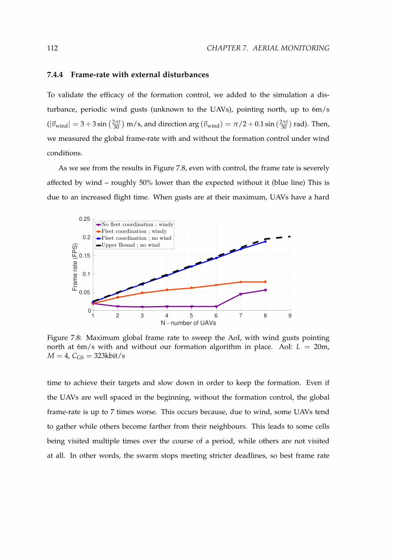
112 CHAPTER 7. AERIAL MONITORING
7.4.4 Frame-rate with external disturbances
To validate the efficacy of the formation control, we added to the simulation a dis-
turbance, periodic wind gusts (unknown to the UAVs), pointing north, up to 6m/s
(|~vwind| = 3+ 3 sin(
2πt30
)
m/s, and direction arg (~vwind) = π/2+ 0.1 sin ( 2πt30 ) rad). Then,
we measured the global frame-rate with and without the formation control under wind
conditions.
As we see from the results in Figure 7.8, even with control, the frame rate is severely
affected by wind – roughly 50% lower than the expected without it (blue line) This is
due to an increased flight time. When gusts are at their maximum, UAVs have a hard
1 2 3 4 5 6 7 8 9
N - number of UAVs
0
0.05
0.1
0.15
0.2
0.25
Fra
me
ra
te (
FP
S)
Figure 7.8: Maximum global frame rate to sweep the AoI, with wind gusts pointingnorth at 6m/s with and without our formation algorithm in place. AoI: L = 20m,M = 4, CGS = 323kbit/s
time to achieve their targets and slow down in order to keep the formation. Even if
the UAVs are well spaced in the beginning, without the formation control, the global
frame-rate is up to 7 times worse. This occurs because, due to wind, some UAVs tend
to gather while others become farther from their neighbours. This leads to some cells
being visited multiple times over the course of a period, while others are not visited
at all. In other words, the swarm stops meeting stricter deadlines, so best frame rate

7.5. MONITORING SUMMARY 113
decreases. We note that our control is particularly useful when the number of UAVs is
low. In the limit of one UAV per cell, this formation control is not even needed.
7.5 Monitoring Summary
In this chapter, we proposed the use of UAVs to build an extendable camera, to provide
an operator a wider image from an AoI than the field of view of a single vehicle without
degrading the image resolution. We showed how the refresh rate of the AoI global frame
is improved by incrementing the number of UAVs in use with adequate controls, as well
as the speed of the wireless links. Furthermore, we showed how a formation control
greatly improves the performance of the system when under external disturbances.


Chapter 8
Drones Software Architecture
The drones we used in our work are inexpensive commercial platforms, namely AR
Drone 2.0 from Parrot (Parrot, 2012). However, in order to support the controls and
communications we put forward in this dissertation, we had to develop a full software
stack with appropriate API at which we called Drone-RK. Despite the name, the vast
majority of the modules run both on drones and on the computer basestation. Except
navigation and actuator modules, and the ones that depend on these two, all other
can run on both computers and drones. Figure 8.1 lies down the list of modules that
create Drone-RK, and their direct dependencies. This chapter describes this software
architecture, focusing on the WiFi communications stack.
8.1 Navigation Data, Actuator and Flight Control
The drone platform runs an auto-pilot independent an closed-source process in back-
ground. This process is responsible to measure and interpret navigation data from the
physical sensors and also to move the drone and apply changes in the motors. Our
software stack communicates with this process by means of two TCP sockets, one to
transmit commands and another to receive new navigation data.
115

116 CHAPTER 8. DRONES SOFTWARE ARCHITECTURE
Autonomous
GPS
Utils
Video
Actuator
NavdataTDMA
Pkt Manager
Keyboard
PDR
DroneRK
AR Config
Flight control
Img Process
Application
Figure 8.1: Drone-RK software is comprised of several modules, spanning from actua-tion and sensing to communications.
Therefore, Drone-RK has two modules named Navdata and Actuator. Navdata is the
module in charge of collecting internal navigation data periodically from the AR.Drone
autopilot and save it into a structure. This includes 3-axis accelerometer data, barometric
altitude, ultras-sound height, 3-axis magnetometer data and a gyroscope. A dedicated
thread constantly reads data from the autopilot and feeds a public structure that other
modules can retrieve from. This structure is protected by a mutex.
Actuator module in conjunction with Flight Control are able to receive and apply
motion commands from any other module such as moving forward/backwards, spin-
ning clockwise or anti-clockwise, going up/down, moving left/right. This also includes
sending emergency shutoff commands, changing the minimum/maximum altitude of
flight, minimum/maximum speed for each direction, and setting the color of the mo-
tor LED lights. A dedicated thread periodically sends the command structure data to
the autopilot. This structure is also protected by a mutex, since multiple modules can

8.2. GPS AND AUTONOMOUS FLIGHT 117
provide simultaneous commands.
8.2 GPS and Autonomous Flight
GPS is the module that receives data from the GPS unit via serial port, and translate
such information into a meaningful location data, such as absolute position and relative
to base position. It is also able to save targets aka GPS waypoints given by the user
or other modules. These waypoints are characterized by latitude, longitude, altitude,
tolerated error (to be considered target-reached) and also maximum speed of flight.
The GPS in use is a differential, lowcost, RTK GPS named Piksi (Switfnav, 2017). It
relies on the use of a fixed GPS (Figure 8.2), from where mobile GPS units (Figure 8.3)
receive extra GPS information to improve their own (differential location). It improves
accuracy by collecting extra information such as the phase of the incoming GPS signals
and the relative difference at two different receivers. These utilize dedicated radios
and respective antennas on the 915Mhz frequency to share such information (visible in
both images). These mobile units are able to retrieve differential GPS data in a NED
coordinate system – north, east, down – measuring the distance in millimeters to the
fixed GPS in these three axis. This system is able to work if and only if there are six or
more satellites in view in common, between fixed and mobile units. In case this is not
achieved, they also provide absolute location – latitude, longitude and altitude. Merging
both metrics above we can obtain a higher quality absolute GPS position assuming the
location of the BS is known with high accuracy.
Autonomous flight module feeds from GPS module and navigation data such as
north-heading to analyze which motion commands are to be given to Actuator module
in order to move the UAV to the current target location. It internally implements a PID
controller.

118 CHAPTER 8. DRONES SOFTWARE ARCHITECTURE
Figure 8.2: Piksi GPS Basestation – This unit is placed at a fixed location before dronestake off. This unit has dedicated power source (red power bank, on the right), a ded-icated radio and antenna (on the middle), and an external GPS antenna, too (on theleft).
Figure 8.3: Piksi GPS on a drone – This unit is mobile and receives data from the fixedGPS unit via dedicated radio, which can be seen in Figure 8.2.

8.3. KEYBOARD 119
8.3 Keyboard
For faster development, drones initiate their code via telnet remote terminal. This way,
a local computer can get access to the remote standard output/input. For this reason, a
keyboard module has been created to allow the user to interact with the running Drone-
RK process at each individual drone. This module is able to read key inputs and provide
hardcoded features such as manual flight w+a+s+d (alike videogame common motion
shortcuts), using up/down arrow to takeoff/land, calibrate sensors, pause/resume (p+r)
autonomous flight, set current position as the current waypoint (0).
This module also allows setting up at new actions dynamically, by giving the user
the option to chose the pair key and function to be called when the key is pressed. The
basestation application also explores this feature to give commands to any drone in the
network.
8.4 Communications
Our communication architecture is a three-tiered design with an Application layer (AL)
on top, a Packet Manager (PM) and our TDMA layer at the bottom.
8.4.1 Application Layer – Video capture and collection
The AL is only accessed at the source and sink devices since these are the only nodes
that are responsible for generating or consuming data. The AL in the source runs the
camera application, dedicated to grabbing video frames directly from the camera device
using the Video and Image Processing modules for that. The frames are fragmented
to fit WiFi packets that are then sent to the PM layer. Each fragment takes attached
a corresponding header for proper identification and later re-assembly of frames at the
sink. The left side of Figure 8.4 shows the activity diagram of the AL on the source node.

120 CHAPTER 8. DRONES SOFTWARE ARCHITECTURE
Call PM_send( , sink_ip)Identify
frame part
Append to current
frame file
[last frame part]
[first frame part]
Close
frame file
Create new
frame file
[else]
Open camera
Grab new frame
[i==n][else]
Divide into n parts: App Pkt
App Pkt
Source (Application Layer) Sink (Application Layer)
Call PM_receive( ) App Pkt [i++]
App Pkt (B)App Pkt (A)
Figure 8.4: Behavior diagrams for the Application Layer running at the Source and Sink.In the Source, the AL is responsible for grabbing camera frames, fragmenting them andsending fragments to the PM layer. In the Sink, the AL does the frame re-assembly. TheAL communicates with the PM layer using PM_send() and PM_receive() functions.
The AL on the sink side just collects frame packets, re-assembles the frames into image
files and hands them to the operator application, for display and/or further processing.
The respective behavior is outlined in the right side of Figure 8.4.
8.4.2 Packet Manager (PM) Layer – Routing
The PM layer (Figure 8.5) is in charge of finding the next hop of an incoming packet,
whether it comes from the upper AL layer or from other node through the lower TDMA
layer. Then, the PM either forwards packets to the TDMA layer to proceed their way
along the network or, for packets meeting their final destination (the Sink in this case),
the PM saves them to an internal queue, for later delivery to the AL.
8.4.3 TDMA Layer – Transmission Shaper
The TDMA layer does the shaping of the outgoing communications to the respective
node TDMA slot and its behavior is explained in detail in Figure 8.6. Basically, whenever
the TDMA slot of a node comes, and during its duration, that node enqueues pending

8.4. COMMUNICATIONS 121
Packet Manager Layer (tx)
PMPkt
Grab oldest packet
Build PM packet: PM Pkt
Find next hop: nxt_ip
(enqueue)
Call TDMA_send( , nxt_ip)PM Pkt
PM Pkt
[I'm sink node][I'm not sink node]
Packet Manager Layer (rx)
Add to Tx Queue Add to Rx Queue
Call TDMA_receive( )PMPkt
(dequeue)
(enqueue)
(dequeue)
(enqueue)
(A) (B)App Pkt
TX Queue
App Pkt App Pkt App Pkt
RX Queue
App Pkt App Pkt App Pkt
App Pkt
App Pkt App Pkt
(C) (D)
Figure 8.5: Packet Manager (PM) layer, routes packets to the next hop, or holds them forthe AL if packets have reached their final destination (Sink). Communicates both withAL (above) and TDMA layers (below).
packets in the wireless card for transmission over the air. Note, however, that a new
packet is only sent to the wireless card when the card informs the TDMA module that
the previous packet has been sent.
Finally, the TDMA layer is also assessing the bandwidth of both upstream and down-
stream links and the PDR of its incoming and outgoing links, to run DVSP or DRP when
desired. Its requests and replies are periodically sent as TDMA packets and filtered at
this layer, being transparent for the layers above.
8.4.4 Encapsulation
Our protocol stack, from the AL to the TDMA layer, is shown in Figure 8.7, which high-
lights the logical packets (protocol data units – PDUs) of each layer with their specific
header information. The header of each layer is only relevant for that layer and accessed
and modified at that layer, only, following good layering practices. Thus, each layer
can be independently modified, or swapped among different implementation options,

122 CHAPTER 8. DRONES SOFTWARE ARCHITECTURE
TDMA Layer (tx)
Grab oldest packet
Build TDMA packet
Add to Rx Queue:
Call socket recvfrom( )
(dequeue)
(enqueue)
(C)
TDMA Pkt
TDMA Pkt
[begin of time slot]Synchronize clock
[else]
UDP Pkt
Measure clock delay
(enqueue) (dequeue)
(D)PM Pkt
TX Queue
PM Pkt PM Pkt PM Pkt
TDMA Layer (rx)
TX Queue
PM Pkt PM Pkt PM Pkt
Call socket sendto( , nxt_ip)TDMA Pkt
PM Pkt
PM Pkt
UDP Pkt
Figure 8.6: TDMA layer is responsible for measuring network delays affecting the in-coming packets. The receiver node adjusts the phase of its own TDMA slot according toany such delays, to keep slots sequential and reduce overlap. Queued packets are onlytransmitted over the air during the TDMA time slot.
without any impact on the remainder of the stack, i.e., in a transparent way. Overall, the
three layers impose an extra 26 byte overhead, which we consider negligible compared
to the payload of 1kB that we are using.
Finally, the TDMA packets are encapsulated into UDP/IP packets. We opted for
UDP instead of TCP to keep better control of the timings of packet transmissions over
the network. We also decided not to do cross-layer optimization, despite some potential
performance improvement that they could bring. The reason was also to strictly enforce
layering, facilitating debugging and future extensions.

8.4. COMMUNICATIONS 123
u16 timestamp ; u32 slot_limits ; u8 slot_id ; u16 req_slot (9 byte)
u64 seq_num ; u8 src ; u8 sink (10 byte)
u8 pkt_type; u16 frame_id ; u8 part_id ; u8 part_total (5 bytes)
Aplication Packet
Pixels
TDMA Packet
PM Packet
UDP Packet
u8 type; u32 seq_num ; u16 timestamp ; u32 slot_limits ; u8 slot_id ; u16 req_slot
u8 type ; u32 seq_num ; u8 src ; u8 sink
u8 type; u16 frame_id ; u8 part_id ; u8 part_total
Aplication Packet
Pixels
TDMA Packet
PM Packet
UDP Packet
(14B)
(7B)
(5B)
Figure 8.7: Our protocol stack, fully respecting the layering principle, with an indepen-dent protocol at each layer using own protocol data units, and final encapsulation in aUDP/IP packet for transport.


Chapter 9
Conclusion
UAVs have never been so ubiquitous as today, and they are enabling a vast set of new
applications such as live-stream inspection and monitoring of large-scale infrastructures.
But the realization of this promising idea lies dependent on the development of mecha-
nism that can efficiently harness the UAV capabilities. Throughout a series of six chap-
ters (Chapter 3 through Chapter 7), we made several contributions and drew several
conclusions that support our claims. Here we wrap the main ideas behind our thesis
and its validation.
9.1 Thesis Validation
In the beginning of our dissertation, we claimed that joint coordination of network
protocol and topology (placement of nodes) will improve user-interactive control of
UAVs for streaming applications in terms of throughput, delay and reliability. To
show the validity of this, we identified the benefits of using multiple UAVs to extend
the reach of the aerial sensor network. We concluded that understanding the UAV-to-
UAV link is the first step to decide the optimal number of relays on a multi-hop network
of UAVs. Then we were able to identify the two major issues of utilizing such networks.
125

126 CHAPTER 9. CONCLUSION
1. First, the need to synchronize the various transmitters to overcome mutual inter-
ference.
2. Second, we found there are asymmetries in link quality of the network and that
these created buffer overflows under heavy utilization.
For the first problem, we proposed a novel and fully distributed self-synchronizing
TDMA protocol (Chapters 3 and 4). For the second one, we offered two different com-
plementary approaches: DVSP (Chapter 5) and DRP (Chapter 6). While the former relies
on adjusting the rate of transmission of the nodes and equalizes links throughput, mini-
mizing end-to-end delay and packet losses, the second second adjusts the position of the
relay nodes to mitigate link asymmetries equalizing the packet losses (the symmetrical
of the PDR) and maximizing end-to-end throughput.
Finally, we showed how to perform vertical monitoring of a given AoI that can be
larger than a single UAV can cover, on top of the relay network studied and developed
in the previous chapters (Chapter 7). We showed how to control a single UAV for that
task and proposed a flexible mechanism to increase area coverage or global frame rate
adding more sensor UAVs.
Along with all this work, we have presented our implementation effort to support all
the previous contributions. This implementation led to the development of Drone-RK,
a software library that allows applications to stream data over multiple relays seam-
lessly (Chapter 8) structured in three main layers, Application, Packet Manager and
TDMA. This library runs on top of Linux and is available at: http://wise.ece.cmu.
edu/redmine/projects/drone-rk/wiki. It includes modules to retrieve navigation data
and control drone motion, as well.

9.2. FUTURE WORK 127
9.2 Future Work
There are multiple lines of future work that go across all the areas covered in this dis-
sertation.
• TDMA – In this work and to simplify TDMA slot assignment, each node has a
dedicated time slot, that is not concurrent with any other. In the future, we expect
to relax this condition and allow some slot re-utilization at the expenditure of a
more complex/dynamic TDMA scheme but with a possible increase in through-
put. Our self-synchronization method is distributed. In the next steps we will
take advantage of the GPS receivers to achieve more precise clock synchronization
to achieve the desired high network utilization. We are already able to measure
PDR in runtime. We intend to use forward error control mechanisms to enhance
reliability.
• DVSP – we expect to extend this protocol to work with multiples sources. These
will demand the common relay of the sources to negotiate with them in order to
balance the load of each.
• DRP – regarding dynamic relay placement, we are currently addressing the solu-
tion of the general case of positioning n relays and proving convergence when op-
erating iteratively. Moreover, determining the optimal number of relays in asym-
metrical conditions is still an open problem. We also intend to expand our line-
topology to other topologies such as mesh, with multiple sources and multiple
sinks.
• DVSP+DRP – in this work, we have studied both protocols in separate; it will be
interesting to study the major benefits of using both simultaneously. It is expected
that DVSP will be able to cope with link asymmetries at the network level, on

128 CHAPTER 9. CONCLUSION
a fast timescale. DRP will be able to remove these asymmetries at the origin by
moving relays, on a slower timescale.
• Experimental validation of the extendable camera is to be studied in the future.
Performing continuous sweeping of a given area has intrinsic value, but it will
be interesting to study how GPS errors, communication latency and errors, and
camera settings will affect the global frame rate at the basestation in regards to
the theoretic one. Finally, we will also explore a smart role assignment policy that
switches UAVs between sensors and relays, providing a compromise between area
of coverage or frame rate and distance from the ground station.
• Another field to be studied is the portability of the Drone-RK to other drone plat-
forms and other robotic platforms. In special, the communications modules were
designed to work in any machine as long as they have WiFi cards; it would be in-
teresting to investigate its multi-hop streaming features on other platforms. We are
currently migrating the code to a network of smart-bicycles. We intend to build
a digital multi-hop broadcasting system to transmit audio between neighboring
cyclists.
Globally, it will be interesting to achieve full vertical integration of all the aspects
covered in this dissertation. In this endeavour, we will seek focus on high level of re-
liability. Robotic systems in general, and drones in particular are inherently sensitive
to flaws. As personally experienced during most experiments and flights, failures dur-
ing mission time are generally catastrophic and result in a crash, and broken hardware.
Reliability guarantees will be worked in the future.
Another generic future line of work regards evaluation of our system by other engi-
neering teams, such as civil engineers. We have already initiated communication with
other research groups to perform a visual inspection of a bridge, in particular its pillars

9.2. FUTURE WORK 129
and the sensors installed on these. We would like to be reviewed in qualitative terms,
on the quality of our system.


Bibliography
Ahmed, N., Kanhere, S. S., and Jha, S. (2013). Utilizing link characterization for improv-
ing the performance of aerial wireless sensor networks. IEEE Journal on Selected Areas
in Communications, 31(8):1639–1649. 19
Asadpour, M., den Bergh, B. V., Giustiniano, D., Hummel, K. A., Pollin, S., and Plattner,
B. (2014). Micro aerial vehicle networks: an experimental analysis of challenges and
opportunities. IEEE Communications Magazine, 52(7):141–149. 20
Asadpour, M., Giustiniano, D., Hummel, K. A., Heimlicher, S., and Egli, S. (2013). Now
or later?: Delaying Data Transfer in Time-critical Aerial Communication. In Proc.
Ninth ACM Conf. Emerg. Netw. Exp. Technol. (CoNEXT), pages 127–132, Santa Barbara,
CA, USA. ACM Press. 20
Banggood (2017). Eachine E013. banggood.com/
Eachine-E013-Micro-FPV-Racing-Quadcopter-With-5_
8G-1000TVL-40CH-Camera-VR006-VR-006-3-Inch-Goggles-p-1182628.html. Ac-
cessed: 01-01-2018. 3
Basagni, S., Petrioli, C., Petroccia, R., and Stojanovic, M. (2010). Choosing the packet
size in multi-hop underwater networks. In OCEANS 2010 IEEE - Sydney, pages 1–9.
IEEE. 18
131

132 BIBLIOGRAPHY
Bohm, A., Lidstrom, K., Jonsson, M., and Larsson, T. (2010). Evaluating CALM M5-
based vehicle-to-vehicle communication in various road settings through field trials.
In Proc. IEEE Local Comput. Netw. Conf. (LCN), pages 613–620, Denver, CO. IEEE. 19,
25
Cheng, W., Li, M., Liu, K., Liu, Y., Li, X., and Liao, X. (2008). Sweep coverage with mobile
sensors. In Parallel and Distributed Processing, 2008. IPDPS 2008. IEEE International
Symposium on, pages 1–9. 26, 27
CNN (2015). India to use Drones for Crowd Control. https://edition.cnn.com/2015/
04/09/asia/india-police-drones/index.html. Accessed: 01-01-2018. 5
DJI (2017). DJI Mavic Pro. https://www.dji.com/mavic. Accessed: 01-01-2018. 2
Facchinetti, T., Almeida, L., Buttazzo, G. C., and Marchini, C. (2004). Real-time resource
reservation protocol for wireless mobile ad hoc networks. In 25th IEEE International
Real-Time Systems Symposium, pages 382–391. 64
Flushing, E. F., Kudelski, M., Gambardella, L. M., and Di Caro, G. A. (2014). Spatial
prediction of wireless links and its application to the path control of mobile robots. In
Proc. IEEE Int. Symp. Ind. Embed. Syst. (SIES), pages 218–227, Pisa, Italy. IEEE. 24
Forster, C., Lynen, S., Kneip, L., and Scaramuzza, D. (2013). Collaborative monocular
slam with multiple micro aerial vehicles. In 2013 IEEE/RSJ International Conference on
Intelligent Robots and Systems, pages 3962–3970. 16
Fortune (2017). Drone captures images after California wildfire. http://fortune.com/
2017/10/13/drones-california-fires-footage/. Accessed: 01-01-2018. 5
Franco, C. D. and Buttazzo, G. (2015). Energy-aware coverage path planning of uavs. In
Autonomous Robot Systems and Competitions (ICARSC), 2015 IEEE International Confer-
ence on, pages 111–117. 26, 27

BIBLIOGRAPHY 133
Goddemeier, N., Daniel, K., and Wietfeld, C. (2012). Role-based connectivity manage-
ment with realistic air-to-ground channels for cooperative uavs. IEEE Journal on Se-
lected Areas in Communications, 30(5):951–963. 17, 25
Gorain, B. and Mandal, P. S. (2013). Point and area sweep coverage in wireless sensor
networks. In Modeling Optimization in Mobile, Ad Hoc Wireless Networks (WiOpt), 2013
11th International Symposium on, pages 140–145. 26, 27
Gorain, B. and Mandal, P. S. (2014). Approximation algorithms for sweep coverage in
wireless sensor networks. Journal of Parallel and Distributed Computing, 74(8):2699 –
2707. 27
Henkel, D. and Brown, T. X. (2008). Delay-tolerant communication using mobile robotic
helper nodes. In Proc. Int. Symp. Model. Optim. Mobile, Ad Hoc, Wirel. Networks Work.
(WiOPT), pages 657–666, Berlin, Germany. IEEE. 24
Huang, W. H. (2001). Optimal line-sweep-based decompositions for coverage algo-
rithms. In Robotics and Automation, 2001. Proceedings 2001 ICRA. IEEE International
Conference on, volume 1, pages 27–32 vol.1. 26, 28
Intel (2017). Intel Aero Drone. https://click.intel.com/
intel-aero-ready-to-fly-drone.html. Accessed: 01-01-2018. 3, 4
Jia, F., Shi, Q., Zhou, G.-m., and Mo, L.-f. (2010). Packet Delivery Performance in Dense
Wireless Sensor Networks. In Proc. Int. Conf. Multimed. Technol. (ICMT), pages 1–4,
Ningbo, China. IEEE. 18, 25
Li, J., c. Wang, R., p. Huang, H., and j. Sun, L. (2009). Voronoi based area coverage
optimization for directional sensor networks. In Electronic Commerce and Security, 2009.
ISECS ’09. Second International Symposium on, volume 1, pages 488–493. 27

134 BIBLIOGRAPHY
Lindhe, M. and Johansson, K. (2009). Using robot mobility to exploit multipath fading.
IEEE Wirel. Commun., 16(1):30–37. 24
MATLAB (2016). MATLAB Curve Fitting Toolbox. https://www.mathworks.com/
products/curvefitting.html. Accessed: 01-01-2018. 38
Muzaffar, R., Vukadinovic, V., and Cavallaro, A. (2016). Rate-adaptive multicast video
streaming from teams of micro aerial vehicles. In 2016 IEEE International Conference on
Robotics and Automation (ICRA), pages 1194–1201. 20
Nigam, N., Bieniawski, S., Kroo, I., and Vian, J. (2012). Control of multiple uavs for
persistent surveillance: Algorithm and flight test results. IEEE Transactions on Control
Systems Technology, 20(5):1236–1251. 26, 28
Oliveira, L., Almeida, L., and Lima, P. (2015). Multi-hop routing within tdma slots for
teams of cooperating robots. In 2015 IEEE World Conference on Factory Communication
Systems (WFCS), pages 1–8. 51, 52
Parrot (2012). Parrot AR Drone 2.0. http://ardrone2.parrot.com. Accessed: 01-01-
2018. 2, 33, 75, 115
Pinto, L., Moreira, A., Almeida, L., and Rowe, A. (2016a). Aerial multi-hop network
characterisation using cots multi-rotors. In 2016 IEEE World Conference on Factory Com-
munication Systems (WFCS), pages 1–4. 13, 32
Pinto, L. R., Almeida, L., Alizadeh, H., and Rowe, A. (2017a). Aerial video stream
over multi-hop using adaptive tdma slots. In 2017 IEEE Real-Time Systems Symposium
(RTSS), pages 157–166. 13, 51, 59
Pinto, L. R., Almeida, L., and Rowe, A. (2017b). Balancing Packet Delivery to Improve
End-to-End Multi-hop Aerial Video Streaming, pages 807–819. Springer International
Publishing. 13, 83

BIBLIOGRAPHY 135
Pinto, L. R., Almeida, L., and Rowe, A. (2017c). Demo abstract: Video streaming in multi-
hop aerial networks. In 2017 16th ACM/IEEE International Conference on Information
Processing in Sensor Networks (IPSN), pages 283–284. 13, 59
Pinto, L. R., Moreira, A., Almeida, L., and Rowe, A. (2017d). Characterizing multi-
hop aerial networks of cots multirotors. IEEE Transactions on Industrial Informatics,
13(2):898–906. 13, 32, 60, 85
Pinto, L. R., Oliveira, L., Almeida, L., and Rowe, A. (2016b). Extendable matrix camera
using aerial networks. In 2016 International Conference on Autonomous Robot Systems
and Competitions (ICARSC), pages 181–187. 13, 95
SIC (2017). Pedrogao aftermatch. sicnoticias.sapo.pt/. Accessed: 01-01-2018. 5
Suzuki, K. A., Kemper Filho, P., and Morrison, J. R. (2012). Automatic battery replace-
ment system for uavs: Analysis and design. Journal of Intelligent & Robotic Systems,
65(1-4):563–586. 27
Switfnav (2017). Piksi RTK GPS. https://www.swiftnav.com/piksi-multi. Accessed:
01-01-2018. 117
Tech, L. (2017). LeddarOne. www.leddartech.com. Accessed: 01-01-2018. 4
Toksoz, T., Redding, J., Michini, M., Michini, B., How, J. P., Vavrina, M., and Vian, J.
(2011). Automated battery swap and recharge to enable persistent uav missions. In
AIAA Infotech@ Aerospace Conference. 27
Tuna, G., Mumcu, T. V., and Gulez, K. (2012). Design strategies of unmanned aerial
vehicle-aided communication for disaster recovery. In High Capacity Optical Networks
and Enabling Technologies (HONET), 2012 9th International Conference on, pages 115–119.
27, 28

136 BIBLIOGRAPHY
Wandeler, E. and Thiele, L. (2006). Optimal tdma time slot and cycle length allocation
for hard real-time systems. In Proceedings of the 2006 Asia and South Pacific Design
Automation Conference, ASP-DAC ’06, pages 479–484, Piscataway, NJ, USA. IEEE Press.
22
Wang, Q., Jaffrès-Runser, K., Xu, Y., Scharbarg, J. L., An, Z., and Fraboul, C. (2017). Tdma
versus csma/ca for wireless multihop communications: A stochastic worst-case delay
analysis. IEEE Transactions on Industrial Informatics, 13(2):877–887. 23
Wireshark (2016). Wireshark. https://www.wireshark.org. Accessed: 01-01-2018. xix,
47, 48
Yang, M., Kim, D., Li, D., Chen, W., Du, H., and Tokuta, A. O. (2013). Sweep-coverage
with energy-restricted mobile wireless sensor nodes. In Wireless Algorithms, Systems,
and Applications, pages 486–497. Springer. 27
Yanmaz, E. (2012). Connectivity versus area coverage in unmanned aerial vehicle net-
works. In Communications (ICC), 2012 IEEE International Conference on, pages 719–723.
26
Zhao, J. and Govindan, R. (2003). Understanding packet delivery performance in dense
wireless sensor networks. In Proc. First Int. Conf. Embed. Networked Sens. Syst. (SenSys),
page 1, Los Angeles, CA, USA. ACM Press. 18, 25

Chapter A
Channel Assessment Model
Proof of Equation 3.17
The ζmax(d) function, described in Equation 3.17 can be derived from the intrinsic prop-
erties of ζh(d), namely: Equation 3.14, Equation 3.15 and Equation 3.16. By using Equa-
tion 3.16b and Equation 3.15, we show that if the network uses x-hops, throughput is
greater than using any higher number of hops (x+n), as long as distance is lower than
dx,x+1:
ζx(d) > ζx+1(d) if d ∈ [0, dx,x+1)
ζx(d) > ζx+n(d) if d ∈ [0, dx,x+n)
dx,x+1 < dx,x+n ∀n ∈ N>x
(A.1)
By using Equation 3.16c and Equation 3.15, we show that if the network uses x-hops,
throughput is greater than using any lower number of hops (x−m), as long as distance
137

138 APPENDIX A. CHANNEL ASSESSMENT MODEL
is higher than dx,x−1:
ζx(d) > ζx−1(d) if d ∈ (dx−1,x,+∞)
ζx(d) > ζx−m(d) if d ∈ (dx−m,x,+∞)
dx−m,x < dx−1,x ∀m ∈ N<x
(A.2)
According to Equation 3.15, dx,x+1 is greater than dx,x−1. So:
From Equation A.1: ζx(d) > ζx+n(d) if d ∈ [0, dx,x+1) ⇒
ζx(d) > ζx+n(d) if d ∈ (dx,x−1, dx,x+1)
From Equation A.2: ζx(d) > ζx−m(d) if d ∈ (dx−1,x,+∞) ⇒
ζx(d) > ζx−m(d) if d ∈ (dx,x−1, dx,x+1)
Yielding: ζx(d) > ζy(d) if d ∈ (dx−1,x, dx,x+1)
(A.3)
∀x, y ∈ N, x 6= y
We proved that ζx(d) is optimal in the interval (dx−1,x, dx,x+1) regarding any other
number of hops in use.
Proof of Equation 3.16a and Equation 3.18
There is a unique intersection point {D, Θ} ∈ R2, where Θ = ζx(D) = ζy(D).
ζx(D) = ζy(D)
Bx
e(β( Dx )
αx) =
By
e(
β(
Dy
)αy)
eβ( Dx )
αx
eβ(
Dy
)αy=
xy
Dα =ln(
xy
)
β(
x(1−α) − y(1−α))
(A.4)
We see now that Equation A.4 has a unique positive real solution. Both numerator
and denominator are strictly negative due to β < 0, y > x, and α > 1. This shows that
inside the domain interval R+0 , those two functions intersect only once at dAB.

139
Proof of Equation 3.16b: x-hops leads to higher throughput than y-hops, if d<dxy
(x<y)
As a consequence of Equation 3.16a, in the domain interval d ∈ [0, do), ζx(d) and ζy(d)
never intersect each other (as long x 6= y). Since ζh(d) is a continuous function, Bolzano’s
intermediate value theorem is applicable. So, Equation 3.16b is true iff there is at least
one point in that domain where ζx(d) is greater than ζy(d), ∀x < y. We know that ζx(0)
is greater than ζy(0), so the proof is completed:
ζx(0) =Bx>
By= ζy(0) (A.5)
Proof of Equation 3.16c: y-hops leads to higher throughput than x-hops, if
d>dxy (x<y)
As a consequence of Equation 3.16a, in the interval d ∈ (D,+∞), ζx(d) and ζy(d) never
intersect each other (as long x 6= y). Since ζh(d) is continuous, we can prove Equa-
tion 3.16c, showing that the derivative of ζy(x) is lower than ζx(d) at d = D, i.e.:
∃1D : ζx(D) = ζy(D)
∂ζx(d)∂d
∣
∣
∣
d=D<
∂ζy(d)∂d
∣
∣
∣
d=D
⇒ ζx(d) < ζy(d)
∀d ∈ (D,+∞)
(A.6)
First, we derive throughput derivative function(
∂ζh(d)∂d
)
:
∂ζh(d)∂d
=∂
∂d
[
Bh
eβ( dh )
αh]
=ζh(d)(
βhhα
dα
)′
=ζh(d)(
βhhα
)
αdα−1
(A.7)

140 APPENDIX A. CHANNEL ASSESSMENT MODEL
Analyzing Equation A.7, we conclude throughput function has a strictly negative
derivative since β ∈ R− and ζh(d), d, α,∈ R
+. So, proving that the inequality of deriva-
tives Equation A.6 is true, is equivalent to show that:
(
∂ζx(d)∂d
)
(
∂ζy(d)∂d
)
∣
∣
∣
∣
∣
∣
d=D
> 1 (A.8)
(
∂ζx(d)∂d
)
(
∂ζy(d)∂d
)
∣
∣
∣
∣
∣
∣
d=D
=ζx(D)
(
βxαxα
)
Dα−1
ζy(D)(
βyαyα
)
Dα−1=(y
x
)α−1> 1 (A.9)
Proof of Equation 3.15: ζx(d) intersects ζy(d) at a lower distance than ζx(d)
intersects ζz(d), if x < y < z
To prove that dxy < dxz if y < z, we can show that dxy < dxw, ∀w > y, i.e.. we convert
solution dxw, from Equation 3.18, into a function of w, and prove that dxw is a strictly
increasing function of w ∈ N>x, i.e:
∂(dxw)
∂w=
(
ln(w
x
)
β(
x(1−α) − w(1−α))
)′
=k · wk · ln (x/w) + (wk − xk)
βw(xk − wk)2
, (k = 1 − α)
(A.10)
Since kwk ln (x/w), (wk − xk) and βw(wk − xk)2
are all negative, the proof is com-
plete.

Chapter B
Drone-RK API
We present here the list of functions available by each one of the Drone-RK modules.
B.1 Navdata
int drk_sensor_data_init (void);
int drk_sensor_data_close (void);
/** obtain heading relative to north **/
float drk_heading (void);
vector drk_drone_speed_get (void);
/** printout all sensor data **/
void dump_sensors (void);
double drk_ultrasound_raw (void);
/** Ultrasound altitude reading compensated for tilt **/
double drk_ultrasound_altitude (void);
/** barometric altitude **/
double drk_abs_altitude (void);
/** barometric altitude minus a known groundzero altitude **/
double drk_rel_altitude (void);
/** set groundzero barometric altitude **/
void drk_zero_altitude ( uint16_t dft ) ;
141

142 APPENDIX B. DRONE-RK API
/** Prints and shows a graph of the battery **/
void drk_print_battery (void);
/** return percentage of bat left **/
int drk_get_battery (void);
B.2 GPS
GPS module has dozens of functions. We present here wrappers for the main ones:
/* return lastest gps sample data received */
llh_t drk_gps_data ( void );
/* Check for a GPS fix */
int drk_gps_myfix ( void );
/* Get number of visible sats */
int drk_gps_get_numsats ( void );
/* Calculate the distance between : */
/* two LLH structs */
double drk_gps_distance_between ( llh_t gpsA , llh_t gpsB );
/* current position and a coordinate pair */
double drk_gps_mydistance_to ( llh_t target );
/* Get altitude from GPS */
double gps_get_altitude (void) ;
/* current position and a GPS struct */
double drk_gps_true_bearing (llh_t target );
/* Returns GPS altitude of drone */
double drk_gps_altitude_get (void);
/* Returns ground speed of drone */
double drk_groundSpeed_get (void);
/* Debugging methods */
void drk_gps_print (void);

B.3. FLIGHT CONTROL 143
B.3 Flight Control
It is possible to use a small set of high level wrapper functions to move the drone, as
well as set or remove the emergency state. The list below contains some of the main
functions we developed in that regard, that end up calling Actuator module’s functions.
/** Send a takeoff command , then block for five seconds to wait for
completion **/
void drk_takeoff (void);
/** Send a land command , then read sensor data until landed **/
void drk_land (void);
/** Trigger an emergency shutoff (kill the motors ) **/
void drk_emergency (void);
/** Removes the drone from emergency state **/
int drk_remove_emergency (void);
/** Puts the drone in hover mode , using the camera to stabilize **/
void drk_lockdown_hover (int time);
/** Puts the drone in hover mode , using the camera to stabilize **/
void drk_hover (int time);
/** Combined movement **/
void drk_translate ( float pitch , float roll , float yaw , float gaz , int
time_ms );
/** Rotate to the left **/
void drk_spin_left ( float rate , int time);
/** Rotate to the right **/
void drk_spin_right (float rate , int time);
/**Move forward **/
void drk_move_forward (float rate , int time);
/** Move backward **/
void drk_move_backward ( float rate , int time);
/** Move right **/
void drk_move_right (float rate , int time);
/** Move left **/

144 APPENDIX B. DRONE-RK API
void drk_move_left ( float rate , int time);
/**Fly upward **/
void drk_move_up ( float rate , int time);
/** Fly downward **/
void drk_move_down ( float rate , int time);
B.4 Autonomous Flight
The list of actions available at this module are mainly the following ones:
/** initiates autonomous controller **/
error_t drk_autonomous_init (void);
/** Clean up and close **/
void drk_autonomous_close (void);
/** Pause movement immediately **/
void drk_autonomous_pause (void);
/** Resume flight **/
void drk_autonomous_resume (void);
/** Returns state of flight : PAUSED - no rotor output ; FLYING - flying to
target **/
enum flight_status drk_autonomous_get_state (void);
/** returns the current waypoint target **/
gps_waypoint_t drk_autonomous_get_waypoint (void) ;
/** Gives new waypoint to go; overwrites current waypoint **/
void drk_autonomous_set_waypoint ( gps_waypoint_t in_waypoint
);
/** is drone at target position ? (<= distance_tolerance ) **/
enum target_status drk_autonomous_target_reached (void);
/** print a small ascii map with cur pos , BS , and cur target **/
void drk_print_map (void) ;
/** go to piksi base **/
void drk_autonomous_goBS (void );

B.5. PACKET MANAGER 145
/** shift current target : north , if dist_m > 0 ; south , if dist_m < 0 *
*/
void drk_autonomous_goNorth ( double dist_m );
/** shift current target : east , if dist_m > 0 ; west , if dist_m < 0 **/
void drk_autonomous_goEast ( double dist_m );
/** set PID controller parameters : Kp_? - proportional ; Ki_? -
integral ; Kd_? - differential ; ?_h - horizontal ; ?_v - vertical *
*/
void drk_autonomous_set_PID ( double _kp_h , double _ki_h , double _kd_h ,
double _kp_v );
B.5 Packet Manager
/** init PM module **/
error_t drk_PM_init ( uint8_t my_ip ) ;
/** close the module properly **/
error_t drk_PM_close ( void ) ;
/** send a packet to PM **/
error_t PM_send ( uint8_t sink_IP , uint16_t pkt_len , const void * const
pkt_ptr ) ;
/** print current routing table **/
error_t PM_printRoutingSettings ( void ) ;
/** read a packet in PM Rx queue. Option to block till reception . **/
error_t PM_receive ( pkt_t *pkt , uint8_t blocking ) ;
/** get number of packets in the out - buffer **/
float PM_getTxBufferUse ( void ) ;
/** get number of packets in the in - buffer **/
float PM_getRxBufferUse ( void ) ;
/** set new topology : routing pairs of [sink -IP; next -hop -IP] **/
error_t PM_newTopology ( const pair_ips_t const * topology , int entries )
;

146 APPENDIX B. DRONE-RK API
B.6 PDR
/** feedback my neighbors with the value of PDR from -everyone -to -me **/
error_t PDR_shareWithNeighbors ( void );
/** analyze PDR of a given LINK [OTHER ]-->[ MYSELF ] **/
error_t PDR_estimate ( uint32_t s_num , uint8_t other_IP ) ;
/* Reset/Clean up estimates */
error_t PDR_init (void);
/** parsing a rcvd pdr packet **/
error_t PDR_parsePkt ( const void * const rx_tdmapkt_ptr , uint16_t
num_bytes_read , uint8_t other_IP );
/** get value of pdr from other ip to myself **/
float PDR_get_in ( uint8_t ip ) ;
/** get value of pdr from myself to other ip **/
float PDR_get_out ( uint8_t ip ) ;
B.7 TDMA
These are the main functions that TDMA module implements to be used by any other
module or user.
/** init module : threads , slots , etc **/
error_t drk_TDMA_init ( uint8_t my_id );
/** close and cleanup module **/
error_t drk_TDMA_close ( void ) ;
/** change between TDMA modes: CSMA/ rigidTDMA slots / dynamicTDMA slots
(DVSP) **/
void TDMA_off ( void ); /* aka CSMA */
void TDMA_rigid ( void );
void TDMA_dynamic ( void );
/** Get newly rcvd packets . **/
ssize_t TDMA_receive ( void * pkt_ptr , uint8_t * other_ip ) ;
/** send a packet of any chosen type **/

B.8. VIDEO 147
error_t TDMA_sendAnyPacket ( uint8_t dest_ip , tdma_type_t type , uint16_t
pkt_len ,
const void * const pkt_ptr );
/** send packet of type PM **/
error_t TDMA_send ( uint8_t dest_ip , uint16_t pkt_len , const void * const
pkt_ptr ) ;
/** get buffer status **/
int TDMA_isRxBufferFull ( void ) ;
/** Printout current Tx queue content **/
void TDMA_dumpTxQueue ( void );
/** incorporate a new active slot list - BS sends updates **/
error_t TDMA_newSlotList (const uint8_t * const slot_list , const int len
);
/** return current bandwidth being used in and out **/
bandwidth_t TDMA_getBandwidth ( void ) ;
/** request some slot width to a neighbor - used in DVSP **/
void TDMA_reqSlotWidth ( uint16_t req_ms , uint8_t dst_ip )
B.8 Video
This module is in charge to open the video device desired by the user, and allows its
caller to grab a copy of the latest available frame.
int drk_video_close ( void ) ;
int drk_video_init ( char cam_id ) ;
int drk_video_front_init ( unsigned int h, unsigned int w ) ;
int drk_video_bottom_init ( unsigned int h, unsigned int w ) ;
int grab_frame ( void *p , uint32_t *len ) ;

148 APPENDIX B. DRONE-RK API
B.9 Image Processing
This module is responsible to process the raw UYUY image out of the camera and
converted it as needed by the user. The main functions in use are the following ones,
that allow to extract the black and white component and to sub-sample it into a lower
resolution version of itself.
int UYVY_2_Y ( const uint8_t * const in_uyvy , unsigned long len , uint8_t
* out_gray ) ;
int Y_subsample ( const uint8_t * const in_y , unsigned long len , uint16_t
width , uint8_t *out_sub_y , uint8_t factor ) ;
B.10 Actuator
error_t drk_actuator_init ( void ) ;
error_t drk_actuator_close ( void ) ;
/* Send a command to the drone autopilot */
int drk_send_at_command ( const char * send_command , ... );
/* Play an animated sequence on the LEDs */
int drk_play_LED_animation (enum LED_ANIMATION animation , float
frequency , int duration );
B.11 AR Config
It is possible to configure some settings of the AR Drone. These are the main functions
we use.
/** Maximum pitch / roll angle. Must be between 0 and 0.52 radians **/
int drk_ar_change_max_angle ( float radians );
/** min Altitude of the drone in millimeters . 50 - max **/
int drk_ar_change_min_altitude ( int altitude_mm );
/** Maximum Altitude of the drone in millimeters . 500 - 5000 , or 10000 =
no lim **/

B.12. KEYBOARD 149
int drk_ar_change_max_altitude ( int altitude_mm );
/** Maximum Vertical Speed , in millimeters per second , 200 -2000 **/
int drk_ar_change_max_vertical_speed ( int speed_mm_per_sec );
/** Maximum Yaw Speed , in radians per second , 0.7 - 6.11 **/
int drk_ar_change_max_yaw_speed ( float speed_rad_per_sec );
/** to zero inertial sensors **/
int drk_ar_flat_trim (void);
/** make drone spin a 360 deg to calibrate compass **/
void drk_ar_calibrate_magnetometer (void);
int drk_ar_set_outdoor_flight (void);
int drk_ar_set_indoor_flight (void);
int drk_ar_set_outdoor_hull (void);
int drk_ar_set_indoor_hull (void);
B.12 Keyboard
error_t drk_keyboard_init ( void ) ;
error_t drk_keyboard_close ( void ) ;
error_t drk_keyboard_setKey ( int (* action )(int) , int input , char key );
B.13 Utils
/** get last part of ip , from a struct sockaddr_in **/
uint8_t getOtherIP ( struct sockaddr_in si_other ) ;
/** Get last segment of current IP **/
int16_t getMyIP (void) ;
/** open and return a point to a new file **/
int open_log_file ( const char* const prefix , const char * const
sufix , FILE ** file_p ) ;
/** get struct with current epoch time **/
int getCurrentTime ( struct timespec * temp_time ) ;
/** same , but in fractional single number ( seconds ) **/

150 APPENDIX B. DRONE-RK API
double getEpoch ( void ) ;
/** time since Drone -RK as initiated **/
double drk_elapsedTimeSecs ( void ) ;
/** statistics : **/
int32_t computeMax ( int32_t * array , int64_t n ) ;
int32_t computeMean ( int32_t * array , int64_t n ) ;
int32_t computeStd ( int32_t * array , int64_t n , int32_t average ) ;
int32_t computeMin ( int32_t * array , int64_t n );
/*** math , trigonometry , etc: ***/
double wrapTo360 ( double angle_in_degrees ) ; /* range 0 -360 deg -
double */
float wrapTo360f ( float angle_in_degrees ) ; /* range 0 -360 deg - float
*/
/** convert units **/
double degrees_to_radians ( double degrees );
double radians_to_degrees ( double radians );
/** force creation of semaphore by name **/
int drk_sem_create ( char * sem_name , sem_t ** sem_ptr ) ;
/** clean semaphore by name **/
int drk_sem_cleanup ( char * sem_name , sem_t * sem_ptr ) ;
/** signal safe sem_wait () **/
error_t sem_wait_safe ( sem_t * semaphore_ptr , volatile int * exit_flag );
/** signal safe sem_timedwait () **/
error_t sem_timedwait_safe ( sem_t * semaphore_ptr , volatile int *
exit_flag , useconds_t t_us );
/** terminal setup **/
void drk_restore_termios (void) ;
void drk_setup_termios (void) ;
/** error handling - print human readable msgs **/
void printError ( error_t status ) ;
/** print array in hex form **/
void dumpData ( uint8_t *data , uint16_t len ) ;
/** Signal related **/

B.13. UTILS 151
void unblock_all_signals (void);
void block_all_signals (void);
void unblock_one_signal (int sig);
void block_one_signal (int sig);
/** pair a given function callback to a signal **/
error_t sig_set_action ( void (*cb)(int), int sig);